ucge reports - university of calgary · ucge reports number 20233 ... accommodate these...
TRANSCRIPT

UCGE Reports Number 20233
Department of Geomatics Engineering
Evaluation and Enhancement of the Wide Area Augmentation System (WAAS)
(URL: http://www.geomatics.ucalgary.ca/research/publications/GradTheses.html)
by
Ruben Yousuf
September 2005
i

THE UNIVERSITY OF CALGARY
Evaluation and Enhancement of the Wide Area Augmentation System (WAAS)
by
Ruben Yousuf
A THESIS
SUBMITTED TO THE FACULTY OF GRADUATE STUDIES
IN PARTIAL FULFILLMENT OF THE REQUIREMENTS
FOR THE DEGREE OF MASTER OF SCIENCE
DEPARTMENT OF GEOMATICS ENGINEERING
CALGARY, ALBERTA
September 2005
©Ruben Yousuf 2005
ii

Abstract
The Global Positioning System (GPS) does not satisfy the requirements set by the
Federal Aviation Administration (FAA) for aviation applications at this time. This is
mainly because GPS integrity is not guaranteed and even when selective availability is
off, the vertical accuracy is worse than 10 m (affirmed by the FAA), whereas the aviation
requirements are much more stringent due to safety-of-life measures. In order to
accommodate these requirements for safety-critical systems such as a fleet of commercial
aircraft, the FAA has developed and commissioned the Wide Area Augmentation System
(WAAS) on July 10, 2003. WAAS augments the current GPS constellation by providing
differential corrections to its users, which satisfies aviation navigation requirements in
terms of integrity, availability, accuracy, and continuity. An addition to the current
WAAS configuration is being planned, to better service users in Canada; this extension to
the core network is named the Canadian WAAS (CWAAS). Basically, four more wide-
area reference stations (WRSs) are being planned to be added in Canada, with seamless
operation between the two networks (CWAAS and WAAS). In this research, previous
works into describing and testing these systems will be revisited and an evaluation of the
proposed CWAAS reference stations will also be conducted, with a focus on ionospheric
storm events. Thereafter, the WAAS will be envisioned in a more enhanced form, which
will entail having significantly more stations in its reference network. In this manner, the
ionosphere could be sampled at a higher spatial resolution, therefore improving the
accuracy of the ionospheric model. Results show more than 100% improvements in some
cases for the enhancement as compared to the current WAAS performance, and the value
added by CWAAS is seen through increased accuracy and coverage in Eastern Canada.
iii

Acknowledgements
I wish to express my sincere gratitude to my supervisor, Dr. Susan Skone for her
continued supports and understanding. She has encouraged me to challenge new ideas yet
advised to rethink when I got too ambitious. She has provided the invaluable advices,
opportunities and assistance that greatly enhanced all the researches during my graduate
studies.
I would like to thank some of my colleagues: Natalya Nicholson, Victoria Hoyle, Sudhir
Man Shrestha, Yongjin Moon, Lance de Groot and my friend David McAllister for their
inputs and feedbacks into this thesis. I would also like to acknowledge the continual
support of the faculty and staff members into making this department a higher place of
learning, which has led to accomplishments such as this one.
My appreciation also goes to Dr. Anthea Coster (MIT Haystack Observatory) for
providing the ionospheric truth data and helping with the analysis.
Lastly, I would like to extend my sincere appreciation to my family for their extra-
curricular support. In particular, my mother Robeda Yousuf for listening and being
supporting during hectic times, my father Yousuf Ali for being extra proud of my
achievements and encouraging me to excel further, and my dear sister Imona Yousuf for
always being there by my side. A special recognition goes to a person who has made
contributions that are intangible but invaluable to my career in general.
iv

Table of Contents
Abstract……………………………………………………...…………………….…….iii
Acknowledgements………………………………………………………………….…..iv
Table of Contents…………………………………………………………………….…..v
List of Tables……………………………………………………………………….........ix
List of Figures………………………………………………………………………….....x
Acronyms………..…………………………………………………………………….xviii
1 Introduction………………………………………………………….……………….1
1.1 Background and Objectives...…………………...…………….…………………1
1.2 Objectives……………………………………………………………….….……7
1.3 Thesis Outline………………………………………….…………………...……8
2 The WAAS…………………………………………………………………..………11
2.1 Ionospheric Effects……………………………….……………...………..……11
2.2 Augmenting GPS………………………………………………...………..……15
2.2.1 Standard Positioning Service……………………………...……………..16
2.2.2 GPS Error Sources and Corrections……………………………………...17
v

2.2.3 Ionospheric Delay Observable……...…………...……………………….18
2.2.4 DGPS Concepts………………………………………………………….20
2.2.5 WADGPS and SBAS…………………………………………………….21
2.3 The FAA…………………………………………………..……....……………22
2.4 Technical Overview…………………………………………..….……..………24
2.5 WAAS Components…………………………………….…...…………………27
2.6 WAAS Messages……………………...…………….………….………………29
2.7 Services Offered and Applications……………………….….…………………31
2.7.1 WAAS Aviation Applications…………………………………………...33
2.7.2 WAAS Non-Aviation Applications……………………………………...34
2.8 NAV CANADA………………………………………..………………………36
2.9 The Canadian WAAS……………………………………...…………...………37
2.9.1 Proposed CWAAS Reference Stations………………..…………………38
2.9.2 CWAAS Strategies………………………………………………………40
2.9.3 Expected Benefits………………………………………………..………41
2.10 WAAS Correction Models………………………………..……………………42
2.10.1 Clock Error………………………………………………………………43
2.10.2 Orbital Error………………………………………………..……………44
2.10.3 Ionospheric Error……………………………………………...…………45
2.10.4 WAA Reliability and Integrity………………....………………...………47
2.11 Localization Scheme……………………………………..……………….……51
2.11.1 Localization of Orbital Error……………………………………….……51
2.11.2 Localization of Ionospheric Error…………………….…………….……52
vi

3 WAAS Correction Assessment………………………………………….…………54
3.1 Truth Data………………………………………………………………………55
3.1.1 Precise Clock and Orbit Data……………………………….……………55
3.1.2 Ionospheric Data Derived from Truth Observation………….……..……58
3.2 Broadcast Values………………..………………………...……………………60
3.2.1 Broadcast Clock……………………………………………….…………60
3.2.2 Broadcast Orbit……………………………………………………..……61
3.2.3 Broadcast Ionosphere………………………...…………………………..62
3.3 WAAS Correction Accuracy……………………………..…...………..………64
3.3.1 Methodology behind the retrieval of WAAS Corrections…….…………65
3.3.2 Clock and Orbital Accuracy Result…………………....………………...67
3.3.3 Ionospheric Accuracy Results……………...………………………..…...74
4 Positioning Performance Evaluation of the Current WAAS...…………………102
4.1 WAAS Positioning across North America under Various Ionospheric
Conditions………………………...………..………………………………….103
4.1.1 WADGPS Processing……………………………..…………………....103
4.2 Results of WAAS Positioning Across North America……..………...….……106
4.2.1 WAAS Horizontal and 3D Positioning Accuracies…….……..…..……108
4.2.2 WAAS Positioning Reliability…………………………….…..…..……123
4.3 Comparison of Results with an Independent Study……………..……………125
vii

5 Evaluation of the Enhanced WAAS………..……………………………….……130
5.1 Description of the Ionospheric Model…………………..…………………….131
5.1.1 Ionosphere Polynomial Model Validation.…………………………..…133
5.2 CWAAS Configuration Analysis……………………………………….……138
5.2.1 CWAAS Evaluation in Eastern Canada…………………….…….……139
5.2.2 WAAS/CWAAS Evaluation in North America………………………..146
5.3 Assessment of the Enhanced WAAS…………………………………………150
5.3.1 Observability Improvements for the Enhanced WAAS Network………151
6 Conclusions and Recommendations……………………….………….…………162
6.1 Conclusions…………………………………………………………...………162
6.2 Recommendations…………………………………………………….....……166
Appendix A…………………………………..……………………………………..….168
Appendix B…………………………………..……………………………………..….173
Appendix C…………………………………..……………………………………..….176
Appendix D…………………………………..……………………………………..….179
References…………………………………………………………………………..….182
viii

List of Tables
Table 2.1 WAAS Message Types [US DOT, 1999]………………………………..30
Table 2.2 GPS Augmented Technologies for Aviation [Hanlon and Sandhoo, 1997]
……………………………………………………………………………34
Table 2.3 Site Deployment Dates..…………………………………………………38
Table 3.1 IGS Product List [JPL, 2005]……………………………………………56
Table 3.2 Sample Ephemeris Record [Lachapelle, 2003]………………………….62
Table 3.3 Clock and Orbital Accuracies for Broadcast versus WAAS…………….69
Table 3.4 WAAS VTEC Error Statistics during October 29-31, 2003 at “AMC2”
……………………………………………………………………………88
Table 3.5 Overall WAAS VTEC Accuracy Statistics for November 20, 2003…….93
Table 3.6 VTEC Accuracies for Broadcast vs. WAAS during November 7-10, 2004
at “NANO”……………………………………………………………….98
Table 4.1 Calgary Station Antenna Coordinates [Henriksen, 1997]…………..…..128
Table 4.2 Accuracy Statistics form this and Two Other Independent Studies……129
Table 5.1 Overall HA and VA Positioning Statistics on November 20, 2003 at
Station VALD for Quiet (0000-2000 UT) and Active (2000-2400 UT)
Ionosphere….…………………………………………………………...143
Table 5.2 Overall HA and VA Positioning Statistics for October 2003 Storm Event
at Station “AZCN”……………………….……………………………..159
ix

List of Figures
Figure 1.1 GPS Constellation [NDGPS, 2003]……………………………………….2
Figure 1.2 WAAS Overview [FAA, 2005]……………………………………………4
Figure 1.3a Electron Density Variation………………………………………………..5
Figure 1.3b VTEC Variation [IRI, 2003]………………………………………………5
Figure 2.1 Ionospheric Electron Density Profile [SPARG, 2003]………………...…12
Figure 2.2 Cycle 23 Sunspot Number Prediction (January 2005) [NOAA, 2005].…13
Figure 2.3 Example of Storm Enhanced Density over North America during a
Geomagnetic Storm Event (March 31, 2001) [Skone et al.,
2003]……………………………………………………………...……...14
Figure 2.4 Ionospheric Pierce Point Geometry……………...………………………19
Figure 2.5 Geometry Involved in Deriving the Mapping Function………..………..20
Figure 2.6 Depiction of DGPS basics [NDGPS, 2003]……………………………...21
Figure 2.7 SBAS Overview [NAV CANADA, 2005]………………………………...22
Figure 2.8 WAAS Overview [NAV CANADA, 2005]……………………………….25
Figure 2.9 WAAS Coverage over the CONUS Region [FAA, 2003]……………….26
Figure 2.10 Typical WRS Setup in the WAAS Network [Bunce, 2003].…………….28
Figure 2.11 INMARSAT Coverage [FAA, 2005].……………………………………29
Figure 2.12 Data Block Format [US DOT, 1999].…………………………………....30
Figure 2.13a GPS+GEO 2D Accuracy Histogram……………………………………..32
Figure 2.13b GPS+GEO 3D Accuracy Histogram [Alud, Private Comm.]……………32
Figure 2.14 Furuno GP32 GPS/WAAS receiver (FUGP32) [The GPS Store, 2005]...35
x

Figure 2.15 Map of Proposed CWAAS Reference Stations [MacDonald, Private
Comm.]…………..…………………………………………………....…39
Figure 2.16 CWAAS Stations (circles) Overlaid on the WAAS Network (squares)
[FAA, 2005]………………………………………………………………41
Figure 2.17 WAAS IGP Locations across North America [US DOT, 1999]…………47
Figure 2.18 FAA Published VPL on February 18, 2005 [FAA, 2005]……………..…50
Figure 2.19 Geometry behind the Derivation of the Orbital Error [Yousuf et al., 2005]
……………………………………………………………………………52
Figure 3.1 Example of an SP3 File………………………………………………..…57
Figure 3.2 The CORS Network [CORS, 2005]…………………………………...…58
Figure 3.3 Example of Diurnal Ionospheric Variation………………………………64
Figure 3.4 Flowchart of Methodology to Derive WADGPS Corrections………...…66
Figure 3.5 Clock Accuracy for Broadcast versus WAAS………………………...…68
Figure 3.6 Orbital Accuracy for Broadcast versus WAAS……………………….…68
Figure 3.7 Clock Accuracy for Broadcast versus WAAS on November 7, 2004...…71
Figure 3.8 Orbital Accuracy for Broadcast versus WAAS on November 7, 2004.…72
Figure 3.9 WAAS UDRE Validation for Clock/Orbital Error………………………73
Figure 3.10 WAAS Clock/Orbital Error versus Age of Correction………………..…74
Figure 3.11 Map of Reference Stations used to Generate Ionospheric Truth Data…...76
Figure 3.12 Kp Values for October 29-31, 2003 (NOAA SEC)…………………...…78
Figure 3.13 Time Series Plot of VTEC Truth during October 29-31, 2003 at User
Station “AMC2”………………………………………………………….78
Figure 3.14a Truth VTEC Map (2100-2130 UT, October 29, 2003)………………..…80
xi

Figure 3.14b WAAS VTEC Map (2100-2130 UT, October 29, 2003)……………...…80
Figure 3.14c VTEC Difference Map (2100-2130 UT, October 29, 2003)………….…81
Figure 3.14d WAAS GIVE Map (2100 UT, October 29, 2003)……………………….81
Figure 3.15a Truth VTEC Map (2100-2130 UT, October 30, 2003)…………………..82
Figure 3.15b WAAS VTEC Map (2100-2130 UT, October 30, 2003)……………...…82
Figure 3.15c VTEC Difference Map (2100-2130 UT, October 30, 2003)………….…83
Figure 3.15d WAAS GIVE Map (2100 UT, October 30, 2003)…………………….…83
Figure 3.16a Truth VTEC Map (2200-2230 UT, October 30, 2003)………………..…84
Figure 3.16b WAAS VTEC Map (2200-2230 UT, October 30, 2003)……………...…84
Figure 3.16c VTEC Difference Map (2200-2230 UT, October 30, 2003)………….…84
Figure 3.16d WAAS GIVE Map (2200 UT, October 30, 2003)…………………….…84
Figure 3.17 Time Series Plots (VTEC Truth, WAAS, Error, UIVE) during October 29-
31, 2003 at User Station “AMC2”…………………………………….…86
Figure 3.18 UIVE Estimates vs. VTEC Error during the October 2003 Storm Event at
Station “AMC2”……………………………………………………….…87
Figure 3.19 Time Series of VTEC Truth on November 20, 2003 at Station
"UIUC"…………………………………………………………………..89
Figure 3.20a Truth VTEC Map (1900-1930 UT, November 20, 2003)……………..…90
Figure 3.20b WAAS VTEC Map (1900-1930 UT, November 20, 2003)…………...…90
Figure 3.20c VTEC Difference Map (1900-1930 UT, November 20, 2003)……….…91
Figure 3.20d WAAS GIVE Map (1900 UT, November 20, 2003)………………….…91
Figure 3.21 VTEC Accuracy Comparison on November 20, 2003 at Station
"UIUC"…………………………………………………………………..92
xii

Figure 3.22 Kp Values for November 7-10, 2004 [NOAA SEC, 2005]………………94
Figure 3.23 GPS TEC Map for 2200-2230 UT, November 7, 2004………………….94
Figure 3.24 VTEC Estimates during the November 7-10, 2004 at "NANO"……...…96
Figure 3.25a Truth VTEC Map (2200-2230 UT, November 7, 2004)…………………99
Figure 3.25b WAAS VTEC Map (2200-2230 UT, November 7, 2004)…………….…99
Figure 3.25c VTEC Difference Map (2200-2230 UT, November 7, 2004)………...…99
Figure 3.25d WAAS GIVE Map (2200 UT, November 7, 2004)…………………...…99
Figure 3.26 Map Showing GIVE minus Differenced WAAS VTEC Error…..……..100
Figure 3.27 UIVE Validation for the November 2004 Storm Event at Station
"NANO"…………………..…………………………………………….101
Figure 4.1 WADGPS Processing Flowchart with a Standard Ionospheric Model....105
Figure 4.2 Locations of CORS Reference Stations Used for WAAS Positioning....107
Figure 4.3 WAAS HA and VA during October 29-31, 2003 at Station "AMC2”…109
Figure 4.4a WAAS Horizontal Positioning Accuracies (1900-1930 UT, October 29,
2003)……………………………………………………………………111
Figure 4.4b WAAS Horizontal Positioning Accuracies (1900-1930 UT, October 30,
2003)……………………………………………………………………111
Figure 4.4c WAAS Vertical Positioning Accuracies (1900-1930 UT, October 29,
2003)……………………………………………………………………111
Figure 4.4d WAAS Vertical Positioning Accuracies (1900-1930 UT, October 30,
2003)……………………………………………………………………111
Figure 4.5a WAAS Horizontal Positioning Accuracies (2100-2130 UT, October 29,
2003)……………………………………………………………………112
xiii

Figure 4.5b WAAS Horizontal Positioning Accuracies (2100-2130 UT, October 30,
2003)……………………………………………………………………112
Figure 4.5c WAAS Vertical Positioning Accuracies (2100-2130 UT, October 29,
2003)……………………………………………………………………112
Figure 4.5d WAAS Vertical Positioning Accuracies (2100-2130 UT, October 30,
2003)……………………………………………………………………112
Figure 4.6a WAAS Vertical Positioning Accuracies (2100-2130 UT, October 29,
2003)………………………………………………………...……….…115
Figure 4.6b WAAS 3D Positioning Accuracies (2100-2130 UT, October 30,
2003)………………………………………………………...……….…115
Figure 4.7a WAAS Vertical Positioning Accuracies (2100-2130 UT, October 29,
2003)………………………………...……………………………….…115
Figure 4.7b WAAS 3D Positioning Accuracies (2100-2130 UT, October 30,
2003)……………………………………………………...………….…115
Figure 4.8 WAAS HA and VA on November 20, 2003 at Station "VALD"………116
Figure 4.9a WAAS Horizontal Positioning Accuracies (2000-2030 UT, November 20,
2003)……………………………………………………………………117
Figure 4.9b WAAS Horizontal Positioning Accuracies (1900-1930 UT, November 20,
2003)……………………………………………………………………117
Figure 4.10a WAAS Vertical Positioning Accuracies (1900-1930 UT, November 20,
2003)………………………………………………………...……….…118
Figure 4.10b WAAS 3D Positioning Accuracies (1900-1930 UT, November 20,
2003)………………………………………………………………....…118
xiv

Figure 4.10c WAAS Vertical Positioning Accuracies (2000-2030 UT, November 20,
2003)………………………………………………………...……….…119
Figure 4.10d WAAS 3D Positioning Accuracies (2000-2030 UT, November 20,
2003)………………………………………………………………....…119
Figure 4.11 WAAS Vertical Positioning Accuracies during Ionospherically Quiet
Time…………………………………………………………………….119
Figure 4.12 WAAS HA and VA during November 7-10, 2004 at Station "AMC2”..121
Figure 4.13 WAAS Horizontal Positioning Accuracies (2200-2230 UT, November 7,
2004).………………………………………………………………..….122
Figure 4.14a WAAS Vertical Positioning Accuracies (2200-2230 UT, November 7,
2004).……………………………………………………….…………..123
Figure 4.14b WAAS 3D Positioning Accuracies (2200-2230 UT, November 7,
2004)………………………………………………….……………...…123
Figure 4.15a WAAS Horizontal Positioning Accuracies (2200-2230 UT, October 30,
2003)………………………………………………….……………...…124
Figure 4.15b WAAS Horizontal Protection Level (2200 UT, October 30, 2003)……124
Figure 4.15c WAAS Vertical Positioning Accuracies (2200-2230 UT, October 30,
2003)………………………………………………….……………...…125
Figure 4.15d WAAS Vertical Protection Level (2200 UT, October 30, 2003)………125
Figure 4.16: Test Setup for Three Different WADGPS Services [Cannon et al., 2002]
…………………………………………………………………………..127
Figure 4.17a MPC Receiver Logging WAAS Messages……………………………..128
Figure 4.17b GPS Antenna Receiving WAAS Downlink and GPS Signals……….....128
xv

Figure 5.1 WADGPS Processing Flowchart with a Refined Ionospheric Model.…133
Figure 5.2 Existing (Red) versus Simulated (Blue) WAAS Network……………...135
Figure 5.3a Figure 5.3a: Difference between VTEC for WAAS Ionosphere Model
versus the Polynomial Model at Standard IGPs (0600-0630 UT, October
30, 2003)………………………………………………………………..137
Figure 5.3b Figure 5.3a: Difference between VTEC for WAAS Ionosphere Model
versus the Polynomial Model at Standard IGPs (2100-2130 UT, October
30, 2003)………………………………………………………………..137
Figure 5.4 VTEC Difference between Existing and Simulated WAAS during the
October 2003 Storm Event at Station "AMC2" for all Satellites in
View.……………………………………………………………………137
Figure 5.5 Model Network for CWAAS Assessment in Eastern Canada………….139
Figure 5.6 WAAS HA and VA on November 20, 2003 at Station "VALD"……....142
Figure 5.7 VTEC WAAS vs. Broadcast Accuracy on November 20, 2003 at "UIUC"
…………………………………………………………………………..145
Figure 5.8 Full Configuration of WAAS + CWAAS Model Network…………….147
Figure 5.9 WAAS vs. WAAS + CWAAS Horizontal Positioning Accuracies (2200-
2230 UT, October 30, 2003)………………………………………...….148
Figure 5.10 WAAS vs. WAAS + CWAAS Vertical Positioning Accuracies (2200-
2230 UT, October 30, 2003)……………...…………….………………149
Figure 5.11 WAAS vs. WAAS + CWAAS 3D Positioning Accuracies (2200-2230 UT,
October 30, 2003)………………………………………………..…..…149
xvi

Figure 5.12 Enhanced WAAS Model Network Using 50+ Reference Stations (Blue
Triangles are Stations Modelling Existing WAAS WRSs and Red
Triangles are Additional Model Stations to Densify the Network and
Includes CWAAS RSs)…………………………………………………151
Figure 5.13 Partial Enhanced WAAS Network near the Great Lakes………………152
Figure 5.14 Single Station IPP Distribution Plot……………………………………153
Figure 5.15 Multiple Station IPP Distribution Plot………………………………….153
Figure 5.16 WAAS vs. Enhanced WAAS Horizontal Positioning Accuracies (2300-
2330 UT, October 30, 2003)……………………………………………155
Figure 5.17 WAAS vs. Enhanced WAAS Vertical Positioning Accuracies (2300-2330
UT, October 30, 2003)…………………………….……………………155
Figure 5.18 Map of User “Test” Sites (magenta triangles) Overlaid on top of the
Simulated Reference Stations…………………………………..………156
Figure 5.19 WAAS HA and VA during October 29-31, 2003 at Station "AZCN"…158
xvii

Acronyms
3D Three-Dimension
ANS Air Navigation Service
BRDC Broadcast
CDGPS Canada-wide Differential Global Positioning System
CODE Center for Orbit Determination in Europe
CONUS Continental United States
CORS Continuously Operating Reference Stations
CWAAS Canadian Wide Area Augmentation System
DGPS Differential Global Positioning System
DOT Department of Transportation
DOT Department of Transportation
ECEF Earth Centered Earth Fixed
FAA Federal Aviation Administration
GEO Geosynchronous Satellite
GIVE Grid Ionospheric Vertical Error
GNSS Global Navigation Satellite System
GPS Global Positioning System
HA Horizontal Accuracy
HAL Horizontal Alarm Limit
IGP Ionospheric Grid Point
IGS International GPS Service
xviii

INMARSAT International Maritime Satellite Organization
IONEX Ionosphere Map Exchange
IPP Ionospheric Pierce Point
ISO International Standardization Organization
JPL Jet Propulsion Laboratory
LAAS Local Area Augmentation System
LOS Line-of-Sight
LPV Localizer Performance with Vertical guidance
LSE Least Squares Estimation
MPC Modulated Precision Clock
NAS National Airspace System
NPA Non-Precision Approach
PA Precision Approach
PRC Pseudorange Correction
PRN Pseudo Random Noise
RAIM Receiver Autonomous Integrity Monitoring
RMS Root Mean Square
RMSE Root Mean Square Error
RTCA Radio Technical Commission for Aviation Services
SA Selective Availability
SA Selective Availability
SBAS Satellite Based Augmentation Systems
SED Storm Enhanced Density
xix

SP3 Standard Product 3
SPIM Standard Plasmasphere-Ionosphere Model
SPS Standard Positioning Service
STEC Slant Total Electron Content
SV Space Vehicle
TEC Total Electron Content
TECU Total Electron Content Unit
UDRE User Differential Range Error
UIVE User Ionospheric Vertical Error
UofC University of Calgary
US United States
UT Universal Time
VA Vertical Accuracy
VAL Vertical Alarm Limit
VTEC Vertical Total Electron Content
WAAS Wide Area Augmentation System
WRS Wide-Area Reference Station
xx

Chapter 1
Introduction
1.1 Background
GPS is a space-based radio-navigation system, as shown in Figure 1.1. A minimum of 24
satellites orbit the Earth, in a nearly circular path, at altitudes of more than 20,000 km.
These space vehicles (SVs) provide accurate position, velocity and time information
derived from range measurements. It was originally developed by the United States (US)
Department of Defense (DOD) for military navigation and positioning purposes
[Parkinson and Spilker, 1996]. Since then, the system has emerged into the civilian
community offering a wide-range of applications. This service is available anytime,
1

anywhere in the world and in all weather conditions. The system consists of three
segments: the Space Segment, the Control Segment, and the User Segment. Each of these
segments has specific functions that as a whole provide the users with positioning and
navigation capabilities [Misra and Enge, 2001].
Figure 1.1: GPS Constellation [NDGPS, 2003]
The positioning information is extracted by estimating geometric range between the GPS
receiver and the tracked satellites – a method known as Trilateration. As in any
estimation process, errors are inherent by nature. Thus, GPS has to deal with an error
budget that includes various sources of error, both systematic and stochastic. These errors
directly impact the positioning accuracies offered by the system [Kaplan, 1996]. With the
increasing use of GPS for navigation purposes, the dependability expected from this
system is being taken to new heights (especially by navigation users). For instance, there
is a substantial growth of the use of GPS technology in commercial aviation. However,
standalone GPS will not provide the level of navigation-aid required by the aviation
2

industry. One of the reasons is that GPS integrity is not guaranteed. In aviation, the
vertical component of positioning is the most important. The accuracy offered by GPS in
the vertical is worse than 10 m, while the requirements set by air-traffic regulation
agencies are much more strict. To alleviate the shortcomings of GPS for the purposes of
navigating commercial and private aircrafts, the Federal Aviation Administration (FAA)
has developed and commissioned the Wide Area Augmentation System (WAAS) (Figure
1.2) on July 10, 2003. WAAS is a safety-critical and software-intensive system that
augments the satellite-based GPS constellation to provide users with airborne positions of
adequate integrity, availability, accuracy, and continuity during different phases of flight.
WAAS positioning is achieved by applying the system-provided differential corrections
to the available positioning solution [Hanlon and Sandhoo, 1997].
Relating to WAAS accuracy, it generates a vector of corrections using its ground
reference stations and sends it to users having WAAS compliant receivers. This vector
contains ionospheric, clock and ephemeris corrections that are sent down to the users via
geostationary satellites. Currently, WAAS covers the CONUS area, and Calgary is at the
edge of this coverage. WAAS testing done over the CONUS region in September 2002
produced accuracy performance of 1–2 m horizontal and 2–3 m vertical 95% of the time
[Altshuler et al., 2002].
3

Figure 1.2: WAAS Overview [FAA, 2005]
Even after applying the WAAS corrections, the dispersive ionosphere still remains the
major contributor in the GPS error budget. The ionosphere consists of ionized gases
having free electrons that delay the signals coming from space. In the past 50 years, many
different methods have been devised to model the ionosphere. Each model is application
specific and thus possesses various attributes. One of such model is the Standard
Plasmasphere-Ionosphere Model (SPIM), which is under development for the
International Standardization Organization (ISO). This model entails taking empirically
derived total electron content (TEC) data and fitting an electron density profile on to the
measurements. It is interesting to note that in this model, GPS observations are used as
one of the inputs to this model [Krankowski et al., 2005].
In satellite navigation, only the ionospheric delay is modelled (because the incoming
signal experiences this delay) and not the full characteristics of the ionosphere. In the
GPS community, this modelling is often simply referred to as ionospheric modelling. As
4

such, from this point onward ionospheric delay modelling will be referred to as
ionospheric modelling.
The ionospheric delay is modeled by estimating the TEC in a column of atmosphere
through which the signal travels, and by removing the elevation angle dependence the
delay is modeled as a standard parameter, which is the vertical TEC (VTEC) [Liu and
Gao, 2004]. In theory, VTEC is derived by integrating the electron density in a vertical
column along the signal path, and this quantity varies diurnally, as a function of altitude
and as a function of TEC, as depicted in Figures 1.3a and 1.3b. Estimation of VTEC at
standard ionospheric grid points (IGPs) with 5°x5° spacing and interpolation of these
estimates at desired user locations form the basis of the WAAS augmentation scheme for
ionospheric scheme [Cormier et al., 2005]. Localized scalar differential GPS (DGPS)
corrections (ionospheric, clock and orbit), decoded from WAAS messages, can be
combined and post-processed to be applied to the user station. It was found in several
studies that the final wide area DGPS solution fell well within the WAAS performance
specifications [Cannon et al., 2002].
( )
Figure 1.3a: Elect
December 1, 2002 Lat: 51°, Lon: -114°
ron Density Variation Figure 1.3b: VTEC Variation [IRI, 2003]
5

In Canada, WAAS has definite potential for being used for various navigation
applications. However, its main purpose during inception was to service the CONUS
region, and since there are a few reference stations in Alaska, WAAS coverage is present
in some parts of Western Canada but almost non-existing in the eastern part of the
country [Loh et al., 1995]. Therefore, some of the Canadian wide-area systems may offer
better performance and coverage here in Canada, because their focus is to provide DGPS
services to Canadian users. One of these is the CDGPS Service, which provides reliable
wide-area DGPS (WADGPS) corrections to Canadian users for various applications
[NAV CANADA, 2005]. As well, the original plan to expand the current WAAS network
into Canada is being realized, and this is named the Canadian WAAS (CWAAS).
Basically, four more wide-area reference stations (WRSs) are being added in Canada,
with seamless WAAS operation through the United States into Canada. The coverage in
Eastern Canada would be extended, significantly improving availability, accuracy and
integrity for that region, as will be shown by the results of this study. The core WAAS
network itself is up for improvements. In particular, there are talks by aviation and
transportation authorities that more WRSs are in order; the exact details have yet to be
disclosed [Cormier, 2005].
One of the reasons these improvements are necessary is because of limited capability of
the current WAAS to adequately handle challenging ionosphere conditions. In general,
the WAAS is only able to capture the low frequency behaviours of the ionosphere, both
in the spatial and temporal domains. Thus, it has a tendency to smooth out the high
frequency, isolated and localized features. As a result, during geomagnetic storms this
6

smoothing effect deteriorates the accuracy of the ionospheric corrections and ultimately
causes major degradation in positioning accuracies. There is also a tendency of the
WAAS to underestimate the ionospheric delay, which is of no surprise since smoothing is
actually failing to capture the large values. Consequently, this constant underestimation is
causing a bias in the WAAS data. Scenarios of this shortcoming for WAAS will be
shown and quantified in later chapters of this thesis.
1.2 Objectives
In a previous study done by Yousuf et al. [2005], it has been shown that WAAS
horizontal positioning errors reached up to 25 m and vertical errors sometimes surpassed
the 30 m mark during severly disturbed ionospheric times. This suggests that WAAS
infrastructure/algorithms do not effectively model the ionosphere during such conditions.
In light of this, ways to reduce the errors due to ionospheric delay should be sought.
Therefore, the intended research will include the following three major objectives:
1. To evaluate the accuracy of the current WAAS satellite clock, orbit and
ionosphere corrections for a variety of ionospheric conditions.
2. To quantify the current level of positioning accuracy offered by WAAS in the US
and Canada using the standard WAAS ionosphere model for various ionospheric
conditions.
7

3. To investigate the improvements obtainable if the current WAAS network is
augmented with additional reference stations. This will involve modelling the
ionosphere with a greater spatial resolution over North America using additional
stations in Canada and in the US. In addition, this will serve to study the benefits
that would be gained in Canada as a result of adding the proposed CWAAS
reference.
1.3 Thesis Outline
Chapter Two provides an overview of the WAAS. It outlines the major elements that
make up this augmentation system and how these elements viably support the whole
system. This chapter goes into describing the different WAAS messages and how the
correction information is extracted from them. A section discusses the WAAS
localization scheme developed for this study. The discussion is then extended to the
CWAAS, which is an extension of the WAAS network in Canada. It includes a review of
the proposed CWAAS network, a study of the potential merger of the two networks
(WAAS and CWAAS), an analysis of the expected benefits, a discussion on how to
evaluate their performances, and a proposal for a denser reference network to better
model the ionosphere, which would improve the current WAAS performance.
8

Chapter 3 presents an analysis of the WAAS corrections in the correction domain. There
are four major parts to the analysis: the truth data and three individual error sources
(ionosphere, clock and orbit) for which the corrections are generated. Since the
ionospheric error is the most significant and the most difficult to model, a greater focus is
put towards understanding the methodology behind its modelling.
Chapter 4 is dedicated to evaluating the current WAAS in the positioning domain under
various ionospheric conditions. Specific case studies are included; three major storm
events from the past decade are studied, and results are described from various
perspectives such as: spatial, temporal, statistical, and conditional. Important findings
will be extracted from the results to be used as a frame of reference for the enhancements
discussed in the next chapter.
Chapter 5 describes the core methodologies behind the research presented herein. It
presents the methods involved in WAAS enhancements and CWAAS network simulation.
The overall results obtained from conducting this comprehensive evaluation of
WAAS/CWAAS positioning accuracies and of the proposed refinements are also
described in detail. Essentially, it provides extensive statistical information and
discussion on the processed results. Observing interesting features and phenomena within
the data, identifying special relationships between parameters, analyzing characteristics,
and discussing specific enhancement issues will also be a part of this section.
9

Finally, Chapter 6 presents the important conclusions drawn from this research and
provides some recommendations towards making further progress into the study of this
research topic.
10

Chapter 2
The WAAS
2.1 Ionospheric Effects
The ionosphere is a complex part of the atmosphere, existing from about 60 km of
altitude up to several hundreds of kilometres, as shown in Figure 2.1. The ionising
radiations of the sun and energetic particles transported by the solar wind produce
concentration of free electrons especially in the 250-400 km high layer known as the F-
region. This phenomenon results in changes in the refractive index of the medium. Radio
waves over 100 MHz that cross the ionosphere are then refracted and delayed. In the L-
11

band, which corresponds to the GPS frequencies, the delay may reach several tens of
metres [Dai et al., 2003].
Figure 2.1: Ionospheric Electron Density Profile [SPARG, 2003]
Ionospheric effects on satellite-based navigation systems such as GPS are a major
concern and interest of experts of the field across the world. The atmospheric effect of
interest for this study is the ionosphere, its impacts on WADGPS positioning, and viable
mitigation techniques. There are several ionospheric phenomena that have adverse effects
on WADGPS in general; of major concerns are 1) phase and amplitude scintillations
causing loss of lock and navigation capabilities and 2) large gradients (both spatial and
temporal) in electron content. Scintillation mostly affects GPS carrier phase
measurements, which are differentially corrected in LAAS. On the other hand, TEC
gradients affect differential methods, which is the basis for the WAAS correction model.
Therefore, the discussion to follow will focus on TEC gradients [Skone et al., 2003].
12

Large gradients in TEC are characteristic of an event called storm enhanced density
(SED). This is caused by enhanced ionospheric electric fields that are present near the
mid- to high-latitudes during geomagnetically disturbed periods, which can lead to
depletions and enhancements of electron density in this region. These large gradients
(>70 ppm) in TEC can cause large differential ionospheric range errors. This
phenomenon initially develops in the lower latitudes during the afternoon (local time).
This is also associated with geomagnetic storms in the phase of the solar cycle from a few
years ago (Figure 2.2). SED was originally recognized in the early 1990’s with the
Millstone incoherent scatter (IS) radar [Foster et al., 2002; Foster and Vo, 2002] and has
been studied in detail with data from the DMSP and IMAGE satellites, and with TEC
data collected from multiple GPS receivers located across the US and Canada [Coster et
al., 2003a; Coster et al., 2003b].
Figure 2.2 Cycle 23 Sunspot Number Prediction (July 2005) [NOAA, 2005]
13

Analysis of the GPS TEC data shows that during geomagnetic disturbances, ionospheric
electrons are transported from lower latitudes to higher latitudes, redistributing TEC
across latitude and local time (Figure 2.3). Gradients as large as 70 ppm have been
observed at geographic latitudes of 45°-50° in North America by the MIT Haystack
Observatory. SED effects can persist for several hours in this region, and this is a
significant issue for North American DGPS services. As such, for the purpose of this
investigation, processing data will include SED occurrences. Namely, during the past few
years this has been observed in October and November 2003 and to a lesser extent in
November 2004. Later sections of this chapter will discuss the actual processing
methodology for this task [Skone et al., 2003].
Figure 2.3 Example of Storm Enhanced Density over North America during a
Geomagnetic Storm Event (March 31, 2001) [Skone et al., 2003]
14

2.2 Augmenting GPS
As discussed earlier, GPS positioning is based on range measurements from the space-
borne satellites to the receiver. These measurements are made by estimating the travel-
time of the signal coming from each satellite to the receiver. During this transmission, the
signal passes through many different mediums that delay and modify the signal, therefore
corrupting the time interval between transmission and reception of the signal. Of major
importance for satellite positioning are the delays caused by the troposphere and the
ionosphere. The tropospheric delays are reduced using empirically derived models (e.g.
the Hopfield Model) and are relatively stable in terms of magnitude [Hopfield, 1969].
The ionosphere (an important element of this research), on the other hand, is much more
difficult to model, especially during geomagnetic storms. As such, it impacts the GPS
error budget very severely [Rodrigues et al., 2004].
The first line of defense against this positioning impedance is applying differential
corrections, which is the basis for DGPS methods. However, sometimes this is not
enough to adequately capture the ionospheric features, and so a more robust method of
ionospheric modelling technique is usually employed; this is known as WADGPS. These
and other topics relating to the augmentation of GPS will be discussed in the following
subsections [Zhang and Bartone, 2004].
15

2.2.1 Standard Positioning Service
A typical GPS user would rely on standard positioning service (SPS), which offers a
horizontal positioning accuracy at the 95th percentile of 22.5 m (assumes average
ionosphere) [Conley, 1998]. This is the guaranteed level of horizontal accuracy offered
by the system at the moment, but prior to May 1, 2000 the accuracy was intentionally
degraded by the US DOD to have greater military control over the system. This was done
by introducing controlled errors (clock dithering) to reduce the precision of SPS. Such
errors could be removed by DOD-authorized users, enabling them to have selective levels
of service; hence, the feature was called Selective Availability (SA) [Misra and Enge,
2001].
The SPS positioning solution is based on the broadcast parameters. These are the clock,
orbital and ionospheric error models that are broadcast through GPS navigation messages,
and the troposphere could be modelled through formulations dependent on
meteorological data. These tropospheric model parameters are derived from previously
made observation of the GPS constellation and the physical surroundings near the
receiver; thus, it is an estimate of the actual occurrences. Post-processing could be done
to further improve the positioning solution, but in that case the real-time element would
be lost. It is to be noted that SPS does not offer the full potential of the service
[Parkinson and Spilker, 1996]. Further mitigation of the errors using various methods and
techniques form the basis of the next few subsections.
16

2.2.2 GPS Error Sources and Corrections
GPS errors basically have three different origins: satellite-based errors, propagation
errors, and receiver-based errors. Of relevance to this research are clock/orbital errors
(satellite-based errors) and ionospheric error (propagation error). The intention herein is
to study and present methods, using which these errors are better modelled and/or
mitigated.
Two main characteristics of any error are magnitude and variability. In Global
Navigation Satellite Systems (GNSS), error variability could depend on temporal and/or
spatial correlation. For instance, clock errors are not strongly correlated, spatially; they
are only dependent on time. On the other hand, the ionospheric error is both spatially and
temporally correlated but very erratic and possesses very localized features. As discussed
above, one way to reduce these errors is to apply the broadcast correction models
provided in the navigation message, but this only removes 50% of the errors. To have a
significant positive impact on the error budget, differential methods should be employed.
In DGPS mode, the corrections for these errors are applied in the positioning domain
[Rodrigues et al., 2004]. The conceptual details on DGPS are given in Subsection 2.2.4.
Atmospheric effects are generally reasonably reduced in DGPS mode. During severe
weather conditions (in case of troposphere) or high levels of ionospheric disturbance,
however, the errors could be significant. The ionospheric range error is a function of the
signal frequency and the electron density along the signal path:
17

23.40f
TECI ±= (in meters) (2.1)
where TEC denotes the total electron content integrated along the signal path (in el/m2), f
is the signal frequency (in Hz), and + (-) denotes the group delay (phase advance). The
ionospheric range error can dominate the DGPS error budget under high levels of
ionospheric activity. Ionospheric range errors can reach up to 25 m in some cases,
whereas typical error level is around 7 m [Lachapelle, 2003]. Additional effects of
ionospheric scintillation can cause degradation of receiver tracking performance and, in
extreme cases, loss of navigation capabilities entirely [Knight et al., 1999].
2.2.3 Ionospheric Delay Observable
An ionospheric pierce point (IPP) is defined as the intersection between a given satellite-
receiver line-of-sight and the thin ionospheric shell. The height of this virtual shell is
nominally taken at 350 km altitude for modelling purposes due to high electron density in
the F region, as discussed in Section 2.1. This is approximated as a shell because the
majority of the ionospheric electrons affecting the GPS signals are concentrated near 350
km altitude. Therefore, it is a suitable representation of the overall ionosphere and, to
minimize the computational burden, only one fixed height is used. Figure 2.4 shows a
schematic of how vertical delay, slant delay, and IPP are related in this thin-shell
approximation.
18

Figure 2.4 Ionospheric Pierce Point Geometry
The actual GPS observations are made in the slant; thus, these have to be mapped to the
vertical. In order to do that, a mapping function is used, which is essentially a factor that
is a function of the elevation angle. Therefore, slant TEC measurements along the
observation line-of-sight can be mapped to the vertical simply by dividing it by this factor.
The inverse of this factor would be used to go from the vertical to slant. The expression
that describes this mapping function is given in Equation 2.2, and the geometry behind
the derivation of this equation is shown in Figure 2.5.
21
22
IPPE
E EcoshR
R1Esin)E(M
−
⎪⎭
⎪⎬⎫
⎪⎩
⎪⎨⎧
⎟⎟⎠
⎞⎜⎜⎝
⎛+
−=′= (2.2)
where E is the satellite elevation angle, RE is the Earth radius, and hIPP is height of the
ionospheric shell.
19

Figure 2.5: Geometry Involved in Deriving the Mapping Function
2.2.4 DGPS Concepts
DGPS involves calculating range errors at a reference station (RS) with its coordinates
known and relaying the error information to remote users within the region of coverage,
as depicted in Figure 2.6. In this manner, orbital and atmospheric errors are reduced,
satellite clock error is eliminated, but receiver noise and Multipath (which is a systematic
error produced by the reflected signals contaminating the direct one) still remain. Various
multipath mitigation techniques exist consisting of proper selection of antenna, receiver
firmware and hardware [Van Dierendonck et al., 1992]. However, solutions could be as
simple as placing the antenna far away from reflective surfaces. Noise, on the other hand,
20

is an inherent error that cannot be eliminated nor reduced, but it can be stochastically
modelled [Zhang and Bartone, 2004].
Figure 2.6: Depiction of DGPS basics [NDGPS, 2003]
2.2.5 WADGPS and SBAS
In wide area differential DGPS (WADGPS), GPS observations from a sparse network of
reference stations are used to model correlated error sources over an extended region.
WADGPS services allow specified minimum levels of positioning accuracy to be
achieved at all locations within the coverage area. With a growing demand for accurate
and reliable DGPS positioning worldwide, several WADGPS services have been
developed in recent years [Cannon and Lachapelle, 1992]. Current operational WADGPS
systems include the WAAS, and commercial WADGPS systems include the OmniSTAR
service.
A space-based augmentation system (SBAS) employs a network of reference stations to
continually collect Global Navigation Satellite System (GNSS) signals coming from the
21

satellites. These reference stations assimilate the dataset and pass it onto the master
station, which in turn processes the incoming raw data and generates the correction and
integrity information for the system. This correction is then fed to the ground uplink
station, which uploads it to the geostationary satellites. Finally, the geostationary
satellites broadcast the correction, integrity, and ranging messages to the users for
navigation augmentation. The schematic in Figure 2.7 depicts the flow of information in
a typical SBAS [NAV CANADA, 2005].
Figure 2.7: SBAS Overview [NAV CANADA, 2005]
2.3 The FAA
The FAA is responsible for the civil aviation in the US. It was originally created under
the name Federal Aviation Agency upon the establishment of the Federal Aviation Act of
1958. Thereafter, it gained its present name (Federal Aviation Administration) when it
22

became a part of the Department of Transportation (DOT) in 1967. FAA’s roles include
regulating civil aviation to promote safety, participating in new aviation and aeronautics
technologies, managing air traffic control, conducting research and development of the
National Airspace System (NAS), and monitoring environmental effects of civil aviation
[FAA, 2005].
FAA’s major activities are as follows [FAA, 2005]:
• Safety Regulation
• Air Space and Air Traffic Management
• Air Navigation Facilities
• Civil Aviation Abroad
• Commercial Space Transportation
• Research, Engineering, and Development
• Organization
• Other Affiliate Programs
As such, FAA overlooks all airspace operations in the US, and throughout the lifespan of
the WAAS, it has definitely added value to FAA’s overall navigation strategies. Since
FAA is the developer and the day-to-day manager of the WAAS, it played an essential
role for this study. Its importance for this research is twofold. Firstly, most of the WAAS
related data used in the processing have been obtained from the FAA, along with
standards and guidelines to follow for proper use of those data products. Secondly, FAA
has been a vital source of information for all the background research on WAAS,
23

provided a frame of reference for the WAAS assessment process and served to establish
the theoretical backbone behind the enhancement.
2.4 Technical Overview
GPS has been put to work for various positioning applications. Nowadays, it is
increasingly being used for navigation purposes. This push to devise more precise and
reliable navigation aids has initiated new research ventures and applications. One of the
major areas of interest for users around the world is aircraft navigation using GPS. This is
mainly because GPS integrity is not guaranteed and even with SA off, the vertical
accuracy is better than 10 m, whereas the aviation requirements are as follows [extracts
from Walter, 2003]:
• Accuracy:
o Less than 7.6 m 95% horizontal and vertical
• Integrity:
o Less than 10-7 probability of true error larger than confidence bound
o 6 second time-to-alarm
• Continuity:
o Less than 10-5 chance of aborting a procedure once it is installed
• Availability:
24

o Horizontal alarm limit (HAL) less than 40 m and vertical alarm limit
(VAL) less than 50 m 95% of the time to 95% of Continental USA
(CONUS), where HAL and VAL are error limits beyond which service
is denied.
In order to accommodate these requirements for safety-critical, the FAA has developed
and commissioned the WAAS (Figure 2.8) on July 10, 2003. The WAAS level of
coverage over the CONUS region is depicted in Figure 2.9 (the percentile values on the
right-hand side represent the coverage level). It consists of [Bunce, 2003]:
• 25 WRSs
• 2 WAAS Master Stations (WMSs)
• 2 Geosynchronous Satellites (GEOs)
• 3 Ground Uplink Stations (GUSs)
Figure 2.8: WAAS Overview [FAA, 2003]
25

Calgary
Figure 2.9: WAAS Coverage over the CONUS Region [FAA, 2003]
WAAS testing done over the CONUS region in September 2002 produced accuracy
performance of 1–2 m horizontal and 2–3 m vertical [FAA, 2005] 95% of the time, which
meets all phases of Category I (Cat I) precision approach. WAAS currently achieves Cat
I approach guaranteed for domestic enroute navigation. The requirements for Cat I are as
follows:
• Vertical positioning accuracy should be 4 m
• Integrity should be guaranteed to 4-8/approach
• Time-to-alarm should be 6 seconds
• VAL should be 12 m
• Continuity should be guaranteed to 1-5/approach
As a result of all the abovementioned upgrades, WAAS current and conceivable benefits
include [extracts from Walter, 2003]:
26

• Primary means of navigation
• More direct routes
• Precision approach capability
• Simplified equipment on-board the aircraft
• Decommission of older and expensive ground equipment
• Improved accuracy and integrity
2.5 WAAS Components
WAAS is comprised of two different segments: the ground segment and the space
segment. The ground segment has three sub-elements: WRS, WMS and GUS. Signals
from GPS satellites are received by the WRSs (Figure 2.10). Each of these precisely
surveyed reference stations receive the signals and determine if errors exist. Each WRS in
the network relays the data to the WMS where correction information is computed. The
WMS calculates correction algorithms and assesses the integrity of the system. A
correction message is prepared and uplinked to a GEOSAT via a ground uplink system
(GUS). The message is then broadcast from the satellite on the same frequency as GPS
(L1, 1575.42 MHz) to receivers onboard aircraft (or any other WAAS capable receiver),
which are within the broadcast coverage area of the WAAS [US DOT, 1999].
27

Figure 2.10: Typical WRS Setup in the WAAS Network [Bunce, 2003]
The space segment consists of two GEOs (there are more to come in 2005) that remain
approximately at a fixed position above the earth. These satellites are the vital links
between the system and the end user. These two International Maritime Satellite
Organization (INMARSAT) communications-relay satellites (called bent-pipes) provide
integrity and ranging corrections [Walter, 2003]. These GEOs have poor ranging
accuracy and vulnerable uplinks. If one of them fails, about half of CONUS will currently
lose coverage until service is restored. Presently, the two satellites serving the WAAS
area are called POR (Pacific Ocean Region) and AOR-W (Atlantic Ocean Region-West)
(Figure 2.11) [FAA, 2005].
28

INMARSAT 3AOR/W54°W
INMARSAT 3POR178°E
INMARSAT 3AOR/W54°W
INMARSAT 3POR178°E
Figure 2.11: INMARSAT Coverage [FAA, 2005]
2.6 WAAS Messages
The navigation information generated and compiled by the WAAS network is relayed to
the user via various messages in Radio Technical Commission for Aviation Services
(RTCA) format. They are received as blocks of data in the form of a bit sequence, as
shown in Figure 2.12. These have specific format, purpose and name. The full set of
WAAS messages are listed in Table 2.1. Basically, the correction information is given
through the message types 2-5, 18, 24 and 25. These and other supporting messages will
be described in detail in later sections, where the WAAS correction models will be
discussed. The remainder of the messages provide various masks, reliability figures, GEO
navigation/almanac data, and status information [US DOT, 1999].
29

24-BITSPARITY212-BIT DATA FIELD
8-BIT PREAMBLE OF 24 BITS TOTAL IN 3 CONTIGUOUS BLOCKS6-BIT MESSAGE TYPE IDENTIFIER (0 - 63)
250 BITS - 1 SECOND
DIRECTION OF DATA FLOW FROM SATELLITE; MOST SIGNIFICANT BIT (MSB) TRANSMITTED FIRST
Figure 2.12: Data Block Format [US DOT, 1999]
Table 2.1: WAAS Message Types [US DOT, 1999]
Type Contents 0 Don't use this GEO for anything (for WAAS testing) 1 PRN Mask assignments, set up to 51 of 210 bits 2-5 Fast corrections 6 Integrity information 7 Fast Correction Degradation factor 8 Estimated RMS Error message 9 GEO navigation message (X, Y, Z, time, etc.) 10 Degradation Parameters 11 Reserved for future messages 12 WAAS Network Time/UTC offset parameters 13-16 Reserved for future messages 17 GEO almanacs message 18 Ionospheric grid point masks 19-23 Reserved for future messages 24 Mixed fast corrections/long term satellite error
corrections 25 Long term satellite error corrections 26 Ionospheric delay corrections 27 Reserved (WAAS Service Message) 28-61 Reserved for future messages 62 Reserved (Internal Test Message) 63 Null Message
30
2.7 Services Offered and Applications
WAAS was conceptualized by FAA to service the civil aviation community by
augmenting various aspects of navigation service for GPS SPS. Its primary objective is
to provide a navigation system for all phases of flight through precision approach. In
order to meet the designated performance requirements, WAAS includes these eight
primary functions [extracts from US DOT, 1999]:
(1) Collect data;
(2) Determine ionospheric corrections;
(3) Determine satellite orbits;
(4) Determine satellite clock corrections;
(5) Determine satellite integrity;
(6) Provide independent data verification;
(7) Provide WAAS message broadcast and ranging; and
(8) Provide system operations and maintenance.
In addition to providing GPS corrections, WAAS supplements the SPS satellite
constellation by GEO ranging. Although the GEO measurement is rather poor due to
limited bandwidth (2 MHz) and use of wide correlator (noisier), overall accuracy does
improve by resorting to these satellites (Figures 2.13a and 2.13b) because more ranging
satellites means more observations are available, and therefore redundant observations
provide a better positioning estimate.
31

For this study, GEO range observations were not used to conduct positioning. The
reason being that positioning solution was computed in post-mission using archived data
from the network of Continuously Operating Reference Stations (CORS), and these
observation data do not include GEO range measurements because CORS receivers are
not WAAS-enabled. Therefore, WAAS corrections were applied independently in the
measurement domain.
0%
10%
20%
30%
40%
50%
60%
70%
80%
90%
100%
0 2 4 6 8 10 12 14 16Position Error (m)
Perc
enta
ge o
f Sam
ples
0%
10%
20%
30%
40%
50%
60%
70%
80%
90%
100%
0 1 2 3 4 5 6Position Error (m)
Perc
enta
ge o
f Sam
ples
GPSGPS+1GeoGPS+2Geos
GPSGPS+1GeoGPS+2Geos
Figure 2.13a: GPS+GEO 2D Accuracy Figure 2.13b: GPS+GEO 3D Accuracy
Histogram Histogram [Alud, Private Comm.]
Since its successful commission in July of 2003, the range of WAAS applications has
grown drastically, from automotive and marine applications to farming and construction
usage. In fact, it is now possible to procure handheld GPS units that support WAAS
positioning, thus offering enhanced accuracy and reliability.
32

2.7.1 WAAS Aviation Applications
The original intent in developing the WAAS, during its inception phase, was to serve the
aviation industry by providing a safe, secure and efficient en-route approach. Since then
its applications have ventured into new horizons. Nonetheless, the focus for FAA
authorities in regulating the WAAS still remains supporting the fleet of commercial
aircrafts. Their continual efforts to support this safety-critical application have shown the
way for other countries (such as Japan, China, India and European countries) to adopt
SBAS methods for augmenting GPS to aid in air-traffic navigation.
There is a major push from the aviation community to allow sole use of GPS for all
phases of flight through Category I precision approach. Clearly, “GPS+” technologies
will need to be incorporated into modern avionic equipment. Some of these technologies
include (but are not limited to) WAAS, GPS with Receiver Autonomous Integrity
Monitoring (RAIM), Local Area Augmentation System (LAAS), and GPS-assisted
inertial systems. A summary of these positioning methods and their corresponding phases
of flight is listed in Table 2.2. Obviously the WAAS plays a big role in all types of non-
precision approaches, as most of the guidance for in-flight operations is provided by
WAAS. The most crucial aspect for WAAS-guided avionic navigation is vertical
positioning, and WAAS is very sensitive about vertical integrity of the system [Shively
and Hsiao, 2004]. In particular, FAA is very swift at denying service to all aviation users
if they sense any indication of deficiencies in integrity. This research attempts to provide
ways to improve these conditions by studying the weaknesses in the current system.
33

Table 2.2: GPS Augmented Technologies for Aviation [Hanlon and Sandhoo, 1997]
Phase of Flight Integrity Availability Accuracy Oceanic GPS with RAIM En Route Domestic Non-precision Approaches
WAAS
Category I Precision Approach WAAS and LAAS Approach & Landing Category II/III Precision
Approach Surface Ground Movement
LAAS
2.7.2 WAAS Non-Aviation Applications
The two major non-aviation applications are navigation on marine and land areas, which
only deal with 2D positioning methods. Figure 2.14 shows a Furuno GP32 GPS/WAAS
receiver (FUGP32) that is used in leisure or fishing boats for marine navigation. Thus,
these types of applications require less stringent integrity and do not involve safety-of-life
circumstances. Users worldwide rely on DGPS and WADGPS systems for a variety of
marine and land applications. These include hydrographic surveying applications, and
exploration/exploitation of marine resources, assistance to vessel traffic management
services, search and rescue operations, environmental assessment and clean-up, and
underwater mine detection and disposal in the marine side. As for land applications,
DGPS and WADGPS systems are being employed in the automotive industry, at
construction sites, for farming needs, and even for recreational purposes. Due to the
diverse nature of these applications, land accuracy requirements are not that regulated
and are very specific to the usage [Yousuf et al., 2005].
34

Figure 2.14: Furuno GP32 GPS/WAAS receiver (FUGP32) [The GPS Store, 2005]
The research conducted herein will also focus on WAAS horizontal positioning, which
pertains to land and marine applications. As well, the proposed Canadian WAAS project
will be investigated, which holds major improvement potentials for marine applications
near the eastern coastlines. In fact the Canadian Coast Guard (CCG) is conducting
feasibility studies on integrating WAAS/CWAAS resources into their own DGPS
services and providing their marine users with WAAS corrections via CCG radiobeacons
[CCG, 2005]. Thus, the research investigations will include an analysis of what the
WAAS has to offer for Canadian marine users and how the CWAAS would further
enhance their horizontal positioning capabilities.
35

2.8 NAV CANADA
NAV CANADA is a non-profit share capital and private corporation that owns and
operates Canada’s civil air navigation service (ANS) by fulfilling various functions. It
operates coast to coast and provides users with air traffic control, flight information,
weather briefings, aeronautical information, airport advisory services and electronic aids
to navigation. NAV CANADA co-ordinates and maintains safety and efficiency of
aircrafts located in Canadian domestic and international airspace assigned to Canadian
control [NAV CANADA, 2005].
NAV CANADA’s infrastructure of ANS facilities includes the following: [extracts
from NAV CANADA, 2005]:
• Area Control Centres
• Terminal Control Units
• Air Traffic Control Towers
• Flight Service Stations
• Community Aerodrome Radio Stations
• Remote Communications Outlets and Remote Aerodrome Advisory Services
• Landing and Navigational Aids
• Radio and Navigational Facilities
• NAV CANADA Training Institute
• Technical Systems Centre
36

In addition, it has over 100 airport control towers and flight service stations. These
facilities are complemented by one stand-alone terminal control unit, 78 Flight Service
Stations, 42 Control Towers, 41 radar sites, a network of 1,400 enroute and terminal
aids to navigation, and landing aids. The provision of safe air navigation services is
NAV CANADA's product and its raison d'être.
2.9 The Canadian WAAS
Recent studies of the WAAS program suggest that its services could be available in
southern Canada [MacDonald, Private Comm.]. The governing body in-charge of this
project is NAV CANADA. It is currently exploring the possibilities of such a
development. Expansion in WAAS infrastructure is the only viable option to that end. It
would consist of fielding additional reference stations strategically located in Canada
feeding measurement information to FAA master stations in the US. This service would,
thus, be called the Canadian WAAS or CWAAS. NAV CANADA and the FAA have
been planning this venture since the mid 1990s. No decision has been made in terms of
funding for CWAAS; such a decision depends on the success of WAAS in application
mode, the compatibility between WAAS master stations and CWAAS station inputs, and
the ability of CWAAS to deliver adequate benefits to aircrafts operating in Canada [NAV
CANADA, 2005].
37

2.9.1 Proposed CWAAS Reference Stations
As was shown in Figure 2.9, WAAS coverage is insufficient in Southeast Canada and the
Northeast United States. Therefore, the joint venture between the FAA and NAV
CANADA is focusing to alleviate this deficiency. NAV CANADA has developed a
mathematical model, based on spatial variability, which can determine if WAAS can
support service in Southern Canada. The same model is used to select optimum locations
for CWAAS reference stations. The model is based on spatial characteristics of the
ionosphere over the region of interest [NAV CANADA, 2005]. NAV CANADA has also
established technical site selection criteria and has evaluated some candidate sites for
suitability. Currently the proposed sites are located in Gander, Goose Bay, Iqaluit and
Winnipeg (Figure 2.15). The project has been approved and the site development and
installation dates are listed in Table 2.3. The station at Gander has been deployed, and
tests are being conducted to ensure proper operability. The remaining stations are still
scheduled to be deployed at the shown dates. It should be noted that FAA is also planning
an expansion of the core WAAS network in the US; the exact details of this expansion
are not fully disclosed by FAA as of yet [MacDonald, Private Comm.].
Table 2.3: Site Deployment Dates
Station Deployment Date
Gander 27-May-05
Goose Bay 29-Sep-05
Iqaluit 17-Aug-06
Winnipeg 11-May-06
38

Figure 2.15: Map of Proposed CWAAS Reference Stations [MacDonald, Private
Comm.]
As can be seen from the figure, improvements attained by adding all or some of the
proposed sites to the network is significant. In particular, the 99% availability of localizer
performance with vertical guidance (LPV) would be extended farther north once full
CWAAS deployment is complete. In terms of coverage, this means that any aircraft
flying south of the green line in Figure 2.15 would have effective vertical guidance from
the WAAS 99% of the time. Thus, WAAS enroute through non-precision approach
coverage would extend to ~65-70°N. As for the regions beyond this coverage, navigation
integrity would be supported using other means. For instance, GPS orbits are such that
receivers at high latitudes can receive signals from satellites over the other side of the
Earth, but GPS signals do not go through the Earth because these signals are in the L-
band of the wave spectrum, which get attenuated by Earth’s surface. Therefore,
GPS/RAIM availability is increased for enroute non-precision approach operations.
39

LAAS would be used for precision approach at these latitudes. Aircrafts operating
through trans-polar routes will most certainly be equipped with GPS-updated inertial
navigation systems that will enable the requirements to be met without CWAAS. The
Precision Approach (PA) navigation mode refers to the navigation solution operating with a
minimum of four satellites with all WAAS corrections (fast-varying, long term, and
ionospheric) available. On the other hand, the Non-Precision Approach (NPA) navigation
mode refers to the navigation solution operating with a minimum of four satellites with fast-
varying and long term WAAS corrections (no WAAS ionospheric corrections) available
[NAV CANADA, 2005].
2.9.2 CWAAS Strategies
NAV CANADA’s CWAAS strategy is as follows [extracts from NAV CANADA, 2005]:
• continue analyzing the potential for WAAS to provide service in Canadian
airspace;
• delay a recommendation to proceed with CWAAS until after the FAA’s
WAAS is proven;
• recommend proceeding with CWAAS only if it will deliver meaningful
benefits to customers;
• buy only proven WAAS hardware and software off the shelf;
• specify a system architecture that delivers maximum benefits at minimum cost
and that is easily adaptable to providing good service with dual-frequency
GPS satellites.
40

2.9.3 Expected Benefits
The foremost benefit to be expected is increased accuracy and coverage for southern
Canada. This is mainly due to the fact that with the inclusion of actual Canadian
reference stations into the WAAS model, the ionospheric spatial features over this region
will be characterized using real observations, and not using a mere mathematical
extrapolation from U.S. sites. Furthermore, larger network will mean better orbit
determination, and therefore, more accurate correction generation for WAAS and
CWAAS users. Augmenting to a larger network has an added benefit of having more
reliable and stable solutions. In other words, outliers would have a lesser weight in
corrupting valid results. The WAAS network supplemented by the envisioned CWAAS
stations is given in Figure 2.16 [NAV CANADA, 2005].
Figure 2.16: CWAAS Stations (circles) Overlaid on the WAAS Network (squares)
[FAA, 2005]
41

2.10 WAAS Correction Models
Multipath and receiver noise are specific to equipment and the surrounding environment.
The troposphere is modelled by the user applying a tropospheric model in real-time using
standard models such as the Hopfield Model, as recommended by WAAS specification
[US DOT, 1999]. WAAS provides corrections for the remaining errors in the following
form: slow clock, slow orbit, fast clock and grid of ionospheric delays. As discussed in
Section 2.6, these corrections are provided using various message types. The ones used
for this research are shown below with their corresponding error/information [Enge et al.,
1996]:
• Type 1: PRN Mask
• Types 2-5: Fast Clock
• Type 18: Ionospheric Grid Point Mask
• Type 24: Mixed Fast/Slow Clock and Orbit
• Type 25: Slow Clock and Orbit and
• Type 26: Ionospheric Delay
Using the above message set, it is possible to derive the appropriate range corrections
corresponding to clock, orbital and ionospheric errors. The subsequent subsections will
review the models enabling the generation of these range corrections.
42

2.10.1 Clock Error
This error is due to imperfections in the synchronization between GPS time and amongst
the satellite clocks. However, this can be modelled using a higher order polynomial as
shown below [US DOT, 1999]:
( ) ( ) ( )202010
ttattaattkfkffkSV
−+−+=∆ (2.3)
where ( )kSV
tt∆ is the total clock correction at time . The , and terms are
the zero, first and second order clock coefficients, respectively, and is an applicable
time of day. Note that in Equation 2.3, the total clock correction value is given in seconds.
Therefore, it must be multiplied by the speed of light to obtain the actual range correction
in metres.
kt
0fa
1fa
2fa
0t
The coefficients are transmitted in the slow clock correction message and are used as
inputs to Equation 2.3 to yield the range correction values. In addition, a set of fast clock
corrections are also sent, as a separate message, to model the high frequency terms.
However, the fast corrections are directly given as scaleable range quantities. The full
(slow + fast) range correction obtained from the messages is generally less than 10 µs (3
m) [Misra and Enge, 2001].
In practice, the polynomial given in Equation 2.3 is only used up to the second term and
sometimes even the second term is omitted depending on the drift rate. A velocity code (1
43

bit in size) is sent along with the coefficient values. This code dictates whether to use this
second term or not. The value of the velocity code is based on a predetermined velocity
threshold. It is true (velocity code has a value of 1) when the threshold is surpassed and
thus the af1 term is used in the equation, and false (code has a value of 0) when it is not
and the af1 term is simply set to 0 [US DOT, 1999].
2.10.2 Orbital Error
The orbital error is caused by inaccuracies in the broadcast model parameters defining the
satellite orbits, and these errors geometrically translate into an error in range and position.
In the WAAS network, the reference and master stations estimate the orbital errors for
given satellites in view and this information is sent to users via the different correction
messages, as described earlier. Magnitudes of the orbital error are typically in the range
of 1-2 m, which could be positive or negative depending on the satellite-receiver
geometry [Lachapelle, 2003]. Corresponding range errors depend on projection of the
orbital error vector along the line-of-sight (LOS) vector from the receiver to the satellite
(refer to Figure 2.19 in Subsection 2.11.1). This orbital error vector (in metres) is given in
the form of a system of linear equations, as show below [US DOT, 1999]:
( )δδδ
δδδ
δδ
δ
xyz
xyz
xy
z
t tk
k
k
k
⎡
⎣
⎢⎢⎢
⎤
⎦
⎥⎥⎥
=⎡
⎣
⎢⎢⎢
⎤
⎦
⎥⎥⎥
+
⎡
⎣
⎢⎢⎢⎢
⎤
⎦
⎥⎥⎥⎥
−
.
.
.0
(2.4)
44

where the orbital error for a given satellite, at time tk , in the x, y and z directions is equal
to the zeroth order error (the most important component of this equation) plus its rate of
change multiplied by the difference between tk and t0 (an applicable time of day). All the
terms present in the right-hand-side of Equation 2.4 are provided through the various
WAAS messages and, by solving the equation, the orbital error vector corresponding to
an individual satellite is found. However, this vector must then be projected along the
appropriate LOS to derive the range error (which is dependent on the location of the
receiver) that could be directly applied as a correction to the raw pseudorange
observation. The basic principles behind the localization of these errors will be given
subsequently in Section 2.11 [US DOT, 1999].
2.10.3 Ionospheric Error
The ionosphere is a major contributor in the GPS error budget. Therefore, its mitigation
will significantly improve positioning accuracy. WAAS attempts to model the
ionospheric delay using dual-frequency GPS measurements from its 25 reference stations
and broadcasts values of ionospheric vertical delay at ionospheric grid points (IGPs) over
its region of coverage, as pictured in Figure 2.17. IGPs are defined to be virtual points
over North America, where the vertical ionospheric delays are estimated by interpolating
the measurements made by the WAAS network. A local planar fit is used to estimate the
vertical delay at each IGP. It is important to note that a different planar fit is imposed at
every IGP using the surrounding local observations [Altshuler et al., 2002].
45

This fit is derived from all the observations within a given radius (R) in North and East
directions. These observations are made by dual-frequency GPS receivers, which enable
the isolation of the ionospheric component because of dispersive nature of the ionosphere.
R may be varied depending on the density of the surrounding observations, but R is
typically 1000 km. If the number of observations within R is less than a preset threshold,
R may be increased until this threshold is surpassed [Altshuler et al., 2002].
VTEC = a0 + a1dE + a2dN (2.5)
where:
VTEC is vertical total electron content
a0, a1, a2 are the planar fit coefficients
dE, dN are distances from the grid points in the East and North
directions, respectively
Using these standard VTEC values, one could compute the ionospheric vertical delay at a
location of interest using the surrounding IGP observations [Altshuler et al., 2002]. This
requires interpolation of the grid points to derive the WAAS grid prediction for a given
user location, which will be discussed in detail in the next section.
46

N75
N65
N55
W180N85
W100W140 W60
N50
Figure 2.17: WAAS IGP Locations across North America [US DOT, 1999]
These ionospheric vertical delay corrections at standard IGPs are provided by WAAS
messages. As well, a reliability indicator called grid ionospheric vertical error (GIVE) is
also given to inform users about model uncertainty. Because WAAS is a safety-critical
system and the ionosphere can be challenging to model, the users are warned about
unreliable data using a set of GIVE flags. Using these standard vertical delay values, one
could compute the ionospheric vertical delay at a location of interest using the
surrounding IGP observations. This requires interpolation between grid points to derive
the WAAS prediction for a given user location, which will be discussed later [US DOT,
1999].
2.10.4 WAAS Reliability and Integrity
WAAS provides IGP ionospheric vertical delay estimates along with associated
reliability indices called the grid ionospheric vertical error (GIVE) values. This is a
47

measure of the error bound provided at each IGP. GIVE flags, ranging between 0 and 15,
are broadcast with associated error and σ2GIVE values (both given in metres) obtained
from a look up table (LUT). The WAAS service provides valid GIVE flags from 0 to 14
(equivalent to a maximum error of 45 m), but when the flag is 15 the service is denied
because the ionosphere is not monitored. This 45 m maximum error is used as a threshold
to account for reliability in the aviation sector. Therefore, basically a grid of vertical
delays and a grid of vertical error bounds are broadcast, which make up the output of the
WAAS ionospheric model. Another index is used to quantify reliability of ionospheric
vertical delay. Namely, the user ionospheric vertical error (UIVE) bounds the residual
(post-correction) pseudorange error and is attributable to the vertical ionospheric delay
for a satellite with a probability of 99.9%. It is interpolated from the surrounding GIVEs
as follows [US DOT, 1999]:
( )∑=
⋅=4
1,
nnppppn GIVEyxWUIVE (2.6)
where xpp and ypp are the coordinates of the user’s IPP for a given satellite and Wn
coefficients are the weight factors, which inversely weigh the distance between the IPP
and IGP.
WAAS also publishes other reliability indicators on a regular basis, and these are the HPL
and VPL estimates. These ensure that post-correction errors are bounded by error bounds
(protection levels) as defined in RTCA/DO-229 Appendix J. Basically, HPL (which has
NPA and PA modes) and VPL are computer from degradation factors and parameters
48

provided in WAAS message Types 7 and 10 [RTCA, 2001]. For details on how to
compute these error bounds and information on the related equations, please refer to the
RTCA document mentioned above.
An example of a published VPL map is given in Figure 2.18. The HPL is the radius of a
circle in the horizontal plane (the plane tangent to the WGS-84 ellipsoid), with its center
being at the true position, which describes the region that is assured to contain the indicated
horizontal position. It is based upon the error estimates provided by WAAS. The VPL is
half the length of a segment on the vertical axis (perpendicular to the horizontal plane of
WGS-84 ellipsoid), with its center being at the true position, which describes the region that
is assured to contain the indicated vertical position. It is based upon the error estimates
provided by WAAS. Accordingly, WAAS guarantees that the user receiver will be within
the error cylinder defined by the horizontal and vertical protection levels [FAA, 2005].
The positioning analyses to be discussed in later chapters will include crosschecks
between the results found and the actual HPL/VPL values published by the FAA.
49

Figure 2.18: FAA Published VPL on February 18, 2005 [FAA, 2005]
Since WAAS is used for safety-critical applications, integrity is a very important element
of the system. In real-time navigation systems, being informed of failures or being
informed late are fatal flaws in system integrity. These issues were closely considered
when developing the WAAS. As a result, it is able to offer a less than 10-7 probability
rate that the true error will be larger than the confidence bound, and the time-to-alarm is
assured to be 6 seconds or less. In terms of continuity, there is a less than 10-5 chance of
aborting a procedure once it is initiated. These along with accuracy and availability
specifications, discussed previously, satisfied the aviation requirements Phase I of PA
navigation mode. There are also Phase II and III, which are related to airport landings
using LAAS and GPS modernization gains. For Phase I, WAAS currently guarantees
reliable positioning at less than 8 m in 3D but typical accuracy is 1-3 m [Walter, 2003].
50

2.11 Localization Scheme
A WAAS localization scheme is implemented here to assess the performance offered by
the system at various locations in North America. The localization scheme has been
tested using such raw data to verify WAAS positioning accuracy at different International
GPS Service (IGS) and CORS stations.
The clock error correction requires no spatial localization. It is a scalar quantity specific
to the satellite, and computing it simply involves using the appropriate clock coefficients
from Equation 2.3. These are provided in the WAAS messages along with the relevant
time tags. Therefore, there are two major parts to this localization scheme: 1) localization
of orbital errors and 2) interpolation of ionospheric delay values for the user station. In
the following subsections, techniques behind the development of the localization scheme
will be discussed.
2.11.1 Localization of Orbital Error
The orbital error requires localization that is based purely on geometry and is also
specific to a given satellite. Figure 2.19 shows the geometrical relationship between the
LOS, the orbital correction vector (δ) and the corresponding pseudorange correction
(PRCorbit).
51

Figure 2.19: Geometry behind the Derivation of the Orbital Error [Yousuf et al.,
2005]
This is basically a scalar projection of δ onto LOS, which results in producing PRCorbit.
The mathematical expression representing this diagram is as follows:
SOLSOLPRCorbit ρ
ρρδ⋅
= (2.7)
The right-hand-side of Equation 2.7 is the dot product between the unit vector along LOS
and δ. This equates to a scalar quantity (in metres) representing the range error and must
be subtracted as an error from the raw pseudorange (as per WAAS convention).
2.11.2 Localization of Ionospheric Error
Localizing the ionospheric correction involves slightly more computation than the other
two error types. First of all, the WAAS broadcasts an evenly-spaced ionospheric grid
52

(nominally 5° spacing at latitudes below 55°) over the footprint of its GEOs (two
currently in operation: POR and AOR-W). GEO coverage exists for most of the US and
the southern parts of Canada, but the WAAS grid actually covers all latitudes across
North America. FAA is currently working towards increasing the GEO coverage, as more
of the GEO satellites will be launched in the near future. The users must then compute
IPPs for each satellite in view and interpolate, from the WAAS grid, their respective
ionospheric delay corrections at each IPP. As discussed earlier, this correction is given as
vertical delay values at the standardized IGPs. Therefore, the interpolated value must be
mapped to the slant path using a mapping function. Three- or four-point interpolation is
suggested depending on the grid spacing and IGP band mask, and this interpolation
method has been used here for all of the processed results for this research. Further
details on the interpolation method and pierce point derivation could be found in US DOT
[1999].
The full WAAS PRC corresponding to all three error components is, therefore, given by:
ionoorbitWAAS PRCPRCPRC ctSV
+⋅∆+= (2.8)
PRCWAAS could now be added to a raw pseudorange value for a given satellite to obtain
the differentially corrected pseudorange. All satellites in view will now have this refined
observable, thus yielding a more accurate positioning estimate of the user’s receiver [US
DOT, 1999].
53

Chapter 3
WAAS Correction Assessment
The chapter will focus on WADGPS corrections that the WAAS broadcasts to its users to
improve positioning accuracy. As discussed previously, there are three types of
corrections: clock, orbit and ionosphere. All these corrections add up to a range quantity,
and thus the raw pseudorange values for each satellite get corrected using these
corrections. Processing these corrected observations produces the final WAAS
positioning solution. Accordingly, the analysis to follow will be conducted in the
correction domain. The study will include discussions on correction schemes, data
sources and formats, validity checks using truth data, integrity checks, and actual case
studies for the correction sets. The ionospheric correction will be studied with great detail,
54

since it causes the major accuracy problems in GPS positioning during ionspherically
disturbed times.
3.1 Truth Data
This section will discuss the sources and methodology behind acquisition and generation
of the truth data for the purposes of validating the WAAS ionospheric, clock and orbital
corrections. The sources have two different origins: 1) precise clock and orbit products
from the IGS website and 2) ionosphere model generated using data from about 400 dual-
frequency GPS reference stations across North America. The analysis is conducted by
comparing the truth data to different sets of results. This comparison entails having two
parts: 1) truth data vs. broadcast data and 2) truth data vs. WAAS data.
3.1.1 Precise Clock and Orbit Data
The data are readily and freely available over the Internet (http://igscb.jpl.nasa.gov/) from
IGS, and no restrictions are placed on using these data for research purposes. Both
precise clock and orbit values are given in single file, which uses a format called
“Standard Product 3” (SP3). A sample file is provided in Figure 3.1. These products are
considered to be precise (less than 0.1 ns), since these are derived by post-processing the
measurements made by the IGS network, which is distributed worldwide. The post-
processing data are sometimes collected over a period of weeks. This extensive spatial
55

coverage combined with the vast temporal redundancy make the final products very
accurate and precise. There are different levels of accuracy for these IGS precise products,
depending on the post-processing time allowed after the fact [JPL, 2005]. There is a
tradeoff between accuracy and latency. As such, IGS also offers rapid products that are
available within a day. A list of the different products and levels of accuracy is given in
Table 3.1.
Table 3.1: IGS Product List [JPL, 2005]
Product Accuracy
Final GPS orbits, 11 days 5 cm
Final SV clocks 0.5 ns
Rapid GPS orbits, 22h 5 – 10 cm
Rapid SV clocks 0.5 – 1.0 ns Predicted GPS orbits, 0h 50 – 100 cm Predicted SV clocks, 0h 80 – 100 ns
56

Figure 3.1: Example of an SP3 File
After the header information, data records are given in time sequence. Each record
provides a time tag with associated orbit and clock information for a given set of satellite
PRN numbers. The true orbits are given as x, y and z coordinates (in km) in the Earth
Centered Earth Fixed (ECEF) frame, while the true satellite clock error is given as a
quantity of time (in µs) [JPL, 2005]. For this study, the selection of the time period is not
critical to the analysis. Therefore, no specific criterion was used to select the truth dataset
over time; consecutive days of SP3 (truth) data were chosen to conduct a temporal
analysis.
57

3.1.2 Ionospheric Data Derived from Truth Observation
The “truth” observations from a network of stations would closely represent actual
ionospheric phenomena. Therefore, the ionospheric truth data were obtained from dual
frequency observations made at about 400 reference stations across North America taken
from the CORS Network, as show in Figure 3.2 [Coster et al., 2003]. Massachusetts
Institute of Technology (MIT) Haystack Observatory provided these absolute slant TEC
observations.
Figure 3.2: The CORS Network [CORS, 2005]
To generate the truth estimates, this network of densely spaced stations is used. All
satellites in view from each station intersect the ionosphere at IPPs (recall the IPP
discussion from Subsection 2.2.3). Each IPP provides a dual-frequency measurement for
the station receiver, but these include inter-frequency (L1/L2) receiver and satellite biases.
The receiver biases are caused by hardware differences in the GPS receiver that processes
the L1 and L2 signals differently, thus yielding an offset in the measurement domain. The
satellite biases, on the other hand, arise mainly as a result of the electronics and antenna
58

on the satellites, which also result in a final measurement offset [McCaskill et al., 2003].
Therefore, it is essential that biases are estimated and removed from the raw observations.
The receiver biases are estimated as part of ionosphere model parameters and are
removed from the observations. The satellite biases, on the other hand, are removed using
published bias values from JPL [JPL, 2005]. An example of a model equation is given by
Equation 3.1, showing the use of a second order polynomial to model the spatial data,
estimation of the biases (if satellite biases are available, then bs would be subtracted from
the right-hand-side of the equation), and mapping of the slant observations to the vertical.
Solving for this type of parametric equation finally produces systematic error-free values,
which can be considered as the truth data. These processed results come in files specific
to the given reference station. These files contain slant TEC values with corresponding
time and PRN tags and other relevant information. As such, the data could be
manipulated as needed for comparison with the counterpart data sets [Coster et al., 2003].
rsirs bbaaaaaaEMtSTEC ++∆∆+∆+∆+∆+∆+= )})(()()()()(){()( 52
42
3210 λφλφλφ
(3.1)
where:
STECrs(ti) is the slant TEC measurement (for receiver r and satellite s) at time ti,
M(E) is a mapping function dependent on elevation angle,
a0… a6 are unknown coefficients of the model,
the constants bs and br are the satellite and receiver inter-channel biases,
59

∆φ is difference in latitude between the IPP and the model expansion point, and
∆λ is difference in longitude [Skone, 2002].
Note: Although this local model was implemented and it produced valid results, this is
just an example of how biases can be estimated and was not used to actually derive the
biases for processing. Instead, the biases were removed using the values provided by
external third parties who estimated the biases conducting a Least-Squares batch solution,
as discussed above.
3.2 Broadcast Values
3.2.1 Broadcast Clock
The broadcast satellite clock error is modelled using a time-dependent polynomial. The
coefficients of this polynomial are transmitted as part of the satellite navigation message.
The computed correlation at time t (in seconds) is given by:
( ) ( ) ( )2210 OCfOCff
ttattaatdt −+−+= (3.2)
where, is the total clock correction at time t . The , and terms are the
zero, first and second order clock coefficients, respectively, and is the time of clock
( )tdt0f
a1f
a2f
a
OCt
60

data. Note that in Equation 3.2, the total clock correction value is given in seconds.
Therefore, it must be multiplied by the speed of light to obtain the actual range correction
in metres.
The coefficients are transmitted as part of the satellite navigation message and are
predicted ahead of time. The full range correction obtained from this input data is
generally less than 1 ms (300,000 m). It is interesting to note that the observed satellite
clock error would be the same for all receivers tracking the same satellites at the same
time, and thus can be eliminated by single differencing between receivers [Misra and
Enge, 2001].
3.2.2 Broadcast Orbit
Similar to clock correction coefficients, the orbital information is provided using a set of
parameters that are transmitted as part of the satellite navigation message. Table 3.2
shows a sample ephemeris record containing all the parameters required to compute the
satellite coordinates and clock error at a given time. The orbital parameters are input into
a set of equations of motion to be solved for the x, y and z coordinates of the satellite (in
metres) in the ECEF frame.
61

Table 3.2: Sample Ephemeris Record [Lachapelle, 2003]
3.2.3 Broadcast Ionosphere
It is a known fact that ionospheric activity varies diurnally and has a sinusoidal trend at
the lowest frequency term. The diurnal maximum occurs at around 14:00 hours local time.
This is why the broadcast ionospheric model was based on the Klobuchar model, which
is basically a half-cosine function given by Equation 3.3 [Klobuchar et al., 1995].
⎟⎠⎞
⎜⎝⎛ −
−=PtADC )(2cos φπτ (3.3)
62

where τ is ionospheric vertical delay (in metres), DC is a constant night-time offset (5
ns), A is amplitude (in metres) of the sinusoid, φ is a constant phase offset (14:00 hours),
t (in seconds) is local time, and finally P is period. [Lachapelle, 2003].
The time-varying coefficients on the right-hand-side of this equation are broadcast in the
GPS navigation message. Therefore, ionospheric vertical delay ( τ ) varies diurnally
according to this sinusoid function, which models the ionospheric activity. Figure 3.3
shows an example of this trend seen over a station in North America. From this figure, it
could be said that the sinusoid function is not modelling the ionosphere adequately in this
intense ionospheric time, as significant local irregularities in the ionosphere are observed.
Thus, predicting functions will fall short of resolving spatial features present during these
phenomena because a low-order smooth model will never capture the higher order effects.
This is especially true for a simple cosine function used in the Klobuchar model, as will
be shown in later chapters [Enge and Van Dierendonck, 1996].
63

Figure 3.3: Example of Diurnal Ionospheric Variation
3.3 WAAS Correction Accuracy
This section will focus on WAAS assessment conducted in the correction domain. To
recap, WAAS correction accuracies were compared to the broadcast ones by subtracting
both from a set of truth data. These truth data were based on precise products obtained
from IGS. There were three types of corrections per data source: clock, orbit and
ionosphere. Since clock and orbital corrections are extracted in a similar manner, these
results will be studied concurrently. Whereas the ionospheric corrections were derived
separately from an alternate source (dual-frequency observation data from about 400
64

reference stations provided by MIT Haystack Observatory), thus this analysis will be
done independently using data from a variety of ionospheric conditions, including
ionospherically disturbed periods.
3.3.1 Methodology Behind the Retrieval of WAAS Corrections
In order to possess the ability to conduct WAAS positioning anywhere in North America,
250-bit raw WAAS frames, that contain all the necessary corrections, for the period of
interest had to be obtained. Thus, these data were procured directly from FAA archives.
This dataset included the relevant messages pertaining to WAAS clock, orbital and
ionospheric error. Thereafter, the 250-bit binary data frames had to be decoded for proper
use. The outputs of the decoder were typical and manageable WAAS messages separated
into the standard WAAS message types (e.g. Type1, Type2, etc.).
At this point, correction information had an ASCII format, and thus was easily readable
by people and software routines. These routines involved retrieving the proper correction
information and then passing on to the localization program (see Section 2.11 to review
algorithmic details). The clock corrections required no localization but orbital and
ionospheric ones did. Orbital localization consisted of a projection on to a vector, and the
ionospheric one involved a bi-linear interpolation using the surrounding three or four data
points across a spatial grid. Obviously, for each satellite in view the primary inputs to the
localization scheme were the coordinates of the “user” location and of the satellite in
question, which determined the magnitude of the interpolated correction value.
65

The above steps ultimately produced the WAAS corrections required for the study, and
the other part of the analysis consisted of the corresponding datasets for precise and
broadcast corrections, so that WAAS vs. truth and broadcast vs. truth comparisons can be
conducted. Once the datasets overlapped, it was a matter of time and PRN matching to
find the two sets of accuracies. To recall how truth and broadcast data were acquired and
processed, revisit the previous sections of this chapter. The clock and orbital errors don’t
have any particular significance when it comes to the “user” location. The ionosphere, on
the other hand, offers a great deal of insight into its physical process depending on the
“user” location, especially if the location is right beneath SEDs. As such, for the
ionospheric correction analysis, this criterion was used to make the selections of the sites
to be studied. A flowchart summarizing this methodology is given in Figure 3.4.
Figure 3.4: Flowchart of Methodology to Derive WADGPS Corrections
66

3.3.2 Clock and Orbital Accuracy Results
These corrections are usually broadcast together in a single message. The exception to
this is WAAS clock, which is given in two different messages: one component is long
term (slow) and the other component is fast. On the other hand, clock and orbital
corrections of type broadcast and precise are extracted from their respective single data
records, as discussed earlier in this chapter.
This analysis will entail looking at the big picture then narrowing down to specific
elements of interest. As such, the first thing to observe is the overall time series for the
whole study period. Figure 3.5 shows the clock errors (in metres) for broadcast and
WAAS during November 7-10, 2004. Similarly, Figure 3.6 shows the three-dimension
(3D) orbital error (in metres) for the same period. These were computed using the
methods discussed in Subsection 2.11.1. Although this is an ionospheric storm event, in
terms of clock and orbital errors it could be considered as typical condition, as
ionospheric activity does not affect those errors.
67

312 312.5 313 313.5 314 314.5 315 315.5 316-10
-8
-6
-4
-2
0
2
4
6
8
10Clock Accuracy for Broadcast versus WAAS
2004 Days (UT)
Clo
ck E
rror (
m)
Prec-BrdcPrec-WAAS
Figure 3.5: Clock Accuracy for Broadcast versus WAAS
312 312.5 313 313.5 314 314.5 315 315.5 3160
2
4
6
8
10
12
14
16
18
20Orbital Accuracy for Broadcast versus WAAS
2004 Days (UT)
3D E
rror (
m) a
t 68t
h-pr
ctile
Prec-BrdcPrec-WAAS
Figure 3.6: Orbital Accuracy for Broadcast versus WAAS
68

As can be seen from these plots, WAAS is definitely more accurate than broadcast for
both clock and orbital cases, in general. However, WAAS has some extreme values (up
to 10 m for clock and up to 18 m for orbit) that are of concern. The statistics representing
the above datasets are summarized in Table 3.3, where again the maxima and minima
appear to be unusual. These instances of large range errors were compared to the
corresponding positioning solutions. It was observed that positioning errors for those
epochs having satellites with outliers were degraded to 5 m as compared to 2 m for
typical WAAS positioning. Therefore, these large inaccuracies were genuinely a product
of the WAAS network.
Table 3.3: Clock and Orbital Accuracies for Broadcast versus WAAS
7-Nov-04 8-Nov-04 9-Nov-04 10-Nov-04
BRDC WAAS BRDC WAAS BRDC WAAS BRDC WAAS
STD 0.72 0.69 0.85 0.47 0.46 0.40 0.53 0.27
RMS 1.83 1.26 2.22 1.24 1.75 1.06 1.67 1.00
MAX 6.12 5.72 9.37 6.42 4.14 4.07 5.87 3.98
Clo
ck (m
)
MIN -2.53 -2.00 -3.60 -4.01 -2.88 -4.60 -1.63 -4.28
MEAN 2.16 1.44 2.18 1.47 2.17 1.33 2.56 1.32
RMS 2.34 2.03 2.48 2.07 2.40 1.80 3.03 1.98
MAX 6.20 15.54 8.42 18.06 6.18 8.13 11.31 18.47
Orb
it (m
)
MIN 0.27 0.13 0.20 0.03 0.22 0.10 0.29 0.09
It was found that if the age of the corrections is significantly large (several minutes) and
if the satellite just came into view of the WAAS network, which would only affect the
orbit prediction, large outliers would exist in the results. In contrast, precise orbits have
69

the advantage of a global IGS network that does not lose sight of the satellites.
Nonetheless, the provided user differential range error (UDRE), which indicates the
99.9% combined fast and slow clock/orbital error for the corrections, should bound the
combined clock and orbital error [Cormier, 2005]. According to these justifications, the
mentioned issues were verified; it was found that the age of correction for the outlying
cases were up to seven minutes, even for the satellites in view; some of the affected
satellites were newly visible by the WAAS network and the corresponding UDREs were
up to 50 m for those cases. Therefore, these outliers are justifiable in terms of
circumstantial occurrences caused by system limitations. A couple of final comments to
be made about the above plots are 1) the fact that no timely trend could be identified,
because clock and orbital errors have no time drifts, and 2) there exists a bias in the clock
correction accuracy (more significant for the broadcast), which is also seen in other
studies done on the topic [Misra and Enge, 2001]. Although, the origin of the biases were
not explicitly discussed in those studies.
The second part of this analysis will focus on observing the range errors for individual
satellites. Specific PRNs were chosen to study both the clock and orbital errors. Shown in
Figures 3.7 and 3.8 are the clock and orbital errors for the given satellites on November 7,
2004. Note that the time interval between two successive data points is 15 minutes
because the precise data were available at that rate. These plots show exact clock and
orbital behaviors over time for the given satellites. As seen in the overall plot and
statistics, the broadcast clock error has a positive bias and the WAAS clock error is
usually non-biased. Although there are occasions, as in the case of PRN 23 in Figure 3.7,
70

where WAAS clock error is significant (up to 5 m) and larger than the broadcast clock
error.
Figure 3.7: Clock Accuracy for Broadcast versus WAAS on November 7, 2004
For the orbital case, WAAS values are generally better except for outliers (seen in PRNs
19 and 22 in Figure 3.8), as discussed above. For the most part, both sets of data have a
parallel error pattern but are vertically offset by some value. In some cases, the two sets
are almost coincident; for instance, the broadcast errors in PRN 28 are very close to the
ones for WAAS. The ionosphere on that day was moderately active, but this should not
affect the orbital corrections. The biases are likely caused by calibration differences
between the source networks.
71

Figure 3.8: Orbital Accuracy for Broadcast versus WAAS on November 7, 2004
In addition to accuracy, reliability is an important aspect of a correction set. As such, it
was necessary to verify if in fact WAAS corrections are bounded reliably, for a given
period of time. For this purpose, the November 7-10 2004 dataset was taken once again
to observe the WAAS UDRE estimates for the whole period for each satellite. This
validation simply involved taking the difference between UDRE and the corresponding
WAAS error, as shown in Figure 3.9. As can be seen, the difference values in this plot
are all positive, which indicates that for this time period the errors in WAAS corrections
were bounded by UDRE at all times. In many instances, extremely large values (100 –
150 m) were observed; it was seen that these usually indicate that satellites have just
72

come into view of the WAAS network. Although, it could be said that WAAS is
somewhat conservative in predicting the UDRE, as the difference values have a
minimum buffer of 15 m and in some cases exceed 200 m.
312 312.5 313 313.5 314 314.5 315 315.5 3160
50
100
150
200
250WAAS UDRE Validation for Clock + Orbital Error
2004 Days (UT)
UD
RE
- E
rror (
m)
Figure 3.9: WAAS UDRE Validation for Clock/Orbital Error
One last aspect of interest in the study of clock/orbital correction is correlation between
accuracy and age of correction. Therefore, WAAS clock/orbital corrections for a given
day (November 9, 2004) were chosen, differenced from the truth, and plotted versus the
correction age in seconds. Figure 3.10 presents the results from this study. There is a
definite correlation between the two elements of interest. As the age of the corrections
becomes larger; thus, a direct relationship in the temporal domain exists for the two
73

quantities. This makes sense because older corrections are less valid at present time than
the more recent ones.
0 50 100 150 200 250 300 350 400 450 50010
12
14
16
18
20
22
24
26
28
30WAAS Clock + Orbital Error vs. Age of Correction
Age of Correction (s)
Erro
r (m
)
Figure 3.10: WAAS Clock/Orbital Error versus Age of Correction
3.3.3 Ionospheric Accuracy Results
The true model of the ionosphere providing the truth data has been generated from a
network about 400 reference stations across North America (station locations shown in
Figure 3.11). The full dataset used to accomplish this task was obtained from MIT
Haystack Observatory. Dual-frequency observations are made by each reference station
to accurately determine the ionospheric delay (slant TEC) to each satellite in view.
Thereafter, the slant observations are mapped to the vertical using a mapping function
74

(refer to Section 2.2) to derive the VTEC values, which are then processed further to
smooth the observations using carrier phase data. Note that the smoothing of the data was
done by the data provider before these were delivered. The receiver and satellite biases
were also removed. Finally, the smooth non-bias VTEC can be considered to be the
ionospheric truth data. There were approximately 612 observations made within the
network per epoch at a sample rate of 90 sec.
The date selection for this study was crucial for the analysis, as the goal is to verify how
the WAAS model performs under various ionospheric conditions. Therefore, specific
ionospheric storm events were chosen to conduct the evaluation. Namely, the October 29-
31, 2003, November 20, 2003 and November 7-10, 2004 events were chosen, where
significant disturbances were observed towards the afternoon (local time). As a result, the
effects of an ionosphere that is quiet versus disturbed could be studied by observing the
diurnal dependence, as well as ability of the WAAS to handle this transition.
75

-160 -150 -140 -130 -120 -110 -100 -90 -80 -70 -6010
20
30
40
50
60
70
80
Longitude (deg)
Latit
ude
(deg
)
Figure 3.11: Map of Reference Stations used to Generate Ionospheric Truth Data
October 29-31, 2003 Storm
One of the highest intensity storms of the past 15 years occurred in late October 2003. A
major solar flare developed at approximately 1100 UT on October 28. A severe
geomagnetic storm commenced in the Earth’s environment at 0600 UT on October 29.
Activity continued for several days, with further coronal mass ejections at approximately
2100 UT October 29 and 1600 UT October 30.
The level of global ionospheric activity during this event is quantified using the
conventional space weather index Kp. This index is based on observations of magnetic
76

field fluctuations at ground-based magnetometer stations (periods of enhanced
ionospheric activity being characterized by strong electric currents which are observed as
magnetic field perturbations at the Earth’s surface). This is a valid method of monitoring
ionospheric activity because strong electric currents signify high electron content, which
drives the ionospheric activity. The planetary Kp index is derived from measurements of
magnetic field variations at thirteen global stations at (approximately) equally spaced
longitudes. This index is derived at three-hourly intervals and values range from 0 (quiet)
to 9 (extreme). Such indices provide an approximate measure of global ionospheric
activity at higher latitudes.
Figure 3.12 shows the Kp index for the full storm period. Kp values of 9 were observed
on October 29 and 30. Figure 3.13 shows the TEC time series for the same period at the
user station “AMC2” (latitude: 38.8031° and longitude: -104.5246°). As can be seen, the
Kp value peaks line up with TEC peaks, which suggests enhancement of ionospheric
TEC during the storm periods, and this indicates severe storm events for extended periods
on both days. Typical diurnal behaviour caused by the ionosphere is could be seen
through the minor peaks in Figure 3.13, where at around mid-day the TEC values peak to
about 5 m. Communications were disrupted for commercial aircraft operating in polar
regions, and satellite instruments were shut down to mitigate the impact of enhanced
radiation in the space environment. Aurora were observed at mid-latitudes – in both
Europe and the United States. Development of strong SED was observed in North
America.
77

Figure 3.12: Kp Values for October 29-31, 2003 (NOAA SEC)
Figure 3.13: Time Series Plot of VTEC Truth during October 29-31, 2003 at User
Station “AMC2”
78

The gradients associated with SED were extremely large during this event. The spatial
distribution of SED over North America is shown in Figure 3.14a for October 29, 2003,
which is also representing the truth data for the given time period. Figure 3.14b is
providing the vertical delay values (in metres, converted using Equation 2.1)
corresponding to the WAAS ionosphere corrections during the same time.
Spatial maps were created to conduct the analysis over North America. These maps
spatially represent the vertical delay distribution for a given time period. These are
derived by taking all the spatial data points for a half-hour batch solution and binning
them into a 2.5° x 2.5° grid-cell; thus, the final cell value for the batch solution is plotted
over the corresponding area. The spatial map in Figure 3.14c shows the difference in
VTEC between the two previous figures; the difference map is simply the subtracted
(WAAS – Truth) image of the two. Figure 3.14d provides the WAAS estimated error
bound for that time frame through its spatially distributed GIVE values. This specific
half-hour interval was chosen for analysis because on October 29 TEC values peak near
the end of the day, and so an interval had to be selected that optimally depicted the
ionospheric intensity during that time.
As can be seen from the truth map, SED is moving across North America. The spatial
series plots in Appendix A shows the SED behaviour. The duration of this phenomenon
was about three hours and caused severe degradation in positioning accuracy and
reliability, as will be shown in later sections. From the WAAS map, it is clear that
WAAS under-estimates TEC values in southern US; this is where the SED effects
79

(featuring steep TEC gradients, fast temporal development, large TEC plume heading
north) are the most pronounced. As a result, the steep TEC gradients cutting across
northwestern US into southwestern Canada are almost not present in the WAAS
estimates, and significant smoothing effect has taken place. This deficiency is best
noticeable in the VTEC difference (WAAS – truth) map. Thus, subtracting the truth
image from WAAS would yield the remaining errors. Clearly, the larger errors (up to 25
m) are located where the SED is most prominent, and these errors are mostly negative,
which again suggests the under-estimation done by the WAAS. Nonetheless, the
difference map is in general non-biased overall for this event. Accordingly, WAAS fails
to fully characterize the ionospheric event pictured in the figures below. The WAAS with
its coarse spatial resolution tends to smooth out the high frequency trends in the data.
Thus, the large valued peaks are modelled by low frequency estimates. This lower bound
approximation ultimately sums up to produce the under-estimation effect.
Figure 3.14a: Truth VTEC Map (2100- Figure 3.14b: WAAS VTEC Map (2100-
2130 UT, October 29, 2003) 2130 UT, October 29, 2003)
80

Figure 3.14c: VTEC Difference Map Figure 3.14d: WAAS GIVE Map (2100
(2100-2130 UT, October 29, 2003) UT, October 29, 2003)
As can be noticed from Figure 3.14d (compared with Figure 3.14c), WAAS errors were
bounded by the GIVE values because these are larger than absolute error values. The
GIVE map also establishes the fact that for most parts of North America, WAAS service
was denied for the period above, as GIVE values exceeded the safe threshold of 45 m
(which is the case in Figure 3.15d but not in 3.14d). An important point to be noted is that
the denial of service only concerns vertical guidance (i.e. aircraft navigation); for WAAS
users dealing in the horizontal and using non-safety-critical applications, the service was
valid. When WAAS ionospheric model become this unreliable, the positioning solution is
then computed using the broadcast model. Thus, WAAS-capable GPS receivers would be
able to provide positioning estimates.
SED effects were also observed on October 30 and were very similar to the occurrences
of October 29. Full development of the event on the 30th is also shown as spatial series
plots in Appendix A. Development of SED persisted during the period 1900-2300 UT.
81

However, the effects were more significant as compared to the previous day, as shown by
Figures 3.15a-d. Unlike in the earlier case, the TEC gradients were steeper and the plume
of high TEC values was wider, but the SED events from both days traveled over the same
regions and showed similar deficiencies in WAAS capability to fully characterize the
phenomenon. TEC values reached up to 30 m for the regions affected by the SED. Once
again, the WAAS TEC values are significantly lower than the truth in terms of magnitude
of the vertical ionospheric delay, especially for the SED regions. Nonetheless, the errors
were once again bounded by WAAS GIVE values.
Figure 3.15a: Truth VTEC Map (2100- Figure 3.15b: WAAS VTEC Map (2100-
2130 UT, October 30, 2003) 2130 UT, October 30, 2003)
82

Figure 3.15c: VTEC Difference Map Figure 3.15d: WAAS GIVE Map (2100
(2100-2130 UT, October 30, 2003) UT, October 30, 2003)
It would be interesting to observe how the SED evolved over time on that day. For this
purpose a consequent half hour time-interval was processed, and the results are below in
Figures 3.16a-3.16d. The main difference between the two intervals, for vertical delay
truth, is the fact that VTEC values are slightly larger corresponding to the SED. However,
in the WAAS map this temporal development of the SED is practically non-existent.
Thus the VTEC errors, as shown in the difference map (Figure 3.16c), are even larger
than the previous half hour period for this day.
83

Figure 3.16a: Truth VTEC Map (2200- Figure 3.16b: WAAS VTEC Map (2200-
2230 UT, October 30, 2003) 2230 UT, October 30, 2003)
Figure 3.16c: VTEC Difference Map Figure 3.16d: WAAS GIVE Map (2200
(2200-2230 UT, October 30, 2003) UT, October 30, 2003)
A temporal analysis is also conducted. Station “AMC2” (black circle in Figure 3.16a)
located directly below the SED was studied closely to observe trends over time. Figure
3.17 presents the results obtained at user station “AMC2”. What are shown are VTEC
truth, WAAS ionosphere corrections, difference between the two and UIVE values over
84

the three days. As seen in the spatial plots above (Figures 3.14a, 3.15a and 3.16a), there
were two major rises in ionospheric delay during this storm period (associated with the
SED), and the two VTEC peaks (on each day) in the figure below indicate those
disturbances. These are seen in the WAAS plot, but the peaks are not significant as
compared to truth observations, especially for the second day. The difference plot is in
support of this fact, in that there is 15 m offset between the maximum errors from the two
days, and on the second day the error is greater. Therefore, it could be said that
ionospheric disturbance reduce the WAAS ability to spatially model the ionosphere. The
last plot in the figure is the UIVE for the period; this is to show that even after
interpolating the GIVE, the errors are still bounded. This could be verified by observing a
scatter plot showing UIVE versus VTEC error (Figure 3.18). The diagonal line in this
plot is separating the Cartesian space into two segments: region where all UIVE values
are less than VTEC errors (upper triangle) and region where all UIVE values are greater
than VTEC errors (lower triangle). Thus, it can be inferred from this figure that for this
dataset UIVE values were always greater than VTEC errors, since all data points lie in
the lower triangle.
85

29 29.5 30 30.5 31 31.50
10
20
30
40
50Tr
uth
Ver
tical
Del
ay (m
)
Vertical Delay and UIVE Estimates during the October 2003 Storm Event at Station "AMC2"
Days in October 200329 29.5 30 30.5 31 31.5
0
10
20
30
40
50
WA
AS
Ver
tical
Del
ay (m
)
Days in October 2003
29 29.5 30 30.5 31 31.5
-20
-10
0
10
20
Ver
tical
Del
ay E
rror (
m)
Days in October 200329 29.5 30 30.5 31 31.5
0
10
20
30
40
50
UIV
E (m
)
Days in October 2003
Figure 3.17: Time Series Plots (VTEC Truth, WAAS Ionosphere Model, Error
(Truth – WAAS), UIVE) during October 29-31, 2003 at User Station “AMC2”
86

Figure 3.18: UIVE Estimates vs. VTEC Error during the October 2003 Storm Event
at Station "AMC2"
A final look at this event was to compute statistics (Table 3.4) of the above dataset, to
derive values for the VTEC errors corresponding to each day. Clearly, October 31
appears to be a relatively quiet day in terms of ionospheric activity. Thus, the
ionospherically quiet versus active days could be compared quantitatively. The daily
variation is clearly seen in the RMS values (computed by taking the root mean square of
all the data points lying within the 24-hour UT boundaries), with the larger errors
occurring on the second day of the storm event. On Oct. 30 the maximum error in WAAS
predicted vertical ionospheric delay climbed to 26 m. Usually, those users relying on the
WAAS for vertical guidance would be denied availability because of large GIVE values
causing such deficiencies in accuracy. WAAS typical performance bounds were
surpassed by a large amount. This is why further refinement of the system is necessary to
adequately handle localized events such as the ones seen above.
87

Table 3.4: WAAS VTEC Error Statistics during October 29-31, 2003 at “AMC2”
Oct. 29 Oct. 30 Oct. 31
MEAN -0.09 0.30 -0.20
RMS 1.67 2.64 0.67
MAX 13.24 26.36 5.01 VTEC
Error (m)
MIN -8.27 -7.42 -6.85
November 20, 2003 Storm
Similarly to the October 2003 storm event, this storm evolved over an extended period of
time (over six hours) but only endured for a single day (November 20). Figure 3.19
depicts the temporal evolution of this storm event. What is shown are VTEC values
obtained from the truth dataset; this shows the temporal evolution of the storm as it was
developing over northeastern US during the course of that day. As can be seen,
interesting features were starting to emerge near the end of the day. At around 1600 UT,
there was a steep increase of the vertical ionospheric delay over the station “UIUC”
(latitude: 40.0990° and longitude: -88.2203°), which is located in northeastern US.
Unlike the October event, these storm effects were observed in the east. This event in
particular is quite unfavorable for users in Eastern Canada, because this area already has
poor WAAS coverage and with the added SED effects, positioning degradations are
substantial. Further investigation of these positioning degradations will be done by
observing this SED from a spatial perspective.
88

Figure 3.19: Time Series of VTEC Truth on November 20, 2003 at Station "UIUC"
The gradients associated with SED were extremely large during this event. The spatial
distribution of SED (truth VTEC map) over North America for November 20, 2003 is
shown in Figure 3.20a, and the corresponding VTEC WAAS, VTEC difference (biases
removed) and GIVE maps are given by Figures 3.20b, 3.20c and 3.20d, respectively.
Note that spatial plots of other time intervals for this event are given in Appendix B. SED
is evolving earlier for this event than the October event, with the larger gradients now
occurring in the central region; this time it is originating in southeastern US and emerging
into southeastern Canada near the Great Lakes area – but similar effects were observed as
in October 2003. In the same manner, for this event WAAS fails to completely resolve
the SED features. Consequently, the difference plot shows an imprint of the SED feature
as large differences in VTEC values, which are still being under-estimated by the WAAS
89

as the SED differenced values are mostly negative; still the errors are bounded by the
GIVE, as can be noticed from Figure 3.20c and then comparing it to Figure 3.20d.
Clearly, most of the GIVE values over North America for this period are about 15 m,
whereas the error level has a maximum at about 12 m; thus, the upper bound is
maintained by the GIVE. Although, a major distinction is that WAAS service was not
denied to any capacity because GIVE values were well below the 45 m threshold.
Another interesting element to note is the noisy characteristic of WAAS vertical delay
estimates in Figure 3.20b. In the previous plots (e.g. from the October 2003 storm event)
it was seen that WAAS estimated values are fairly smooth, spatially; but for this event
this is not the case. It seems that in southeastern US, WAAS ionospheric data have been
corrupted by some kind of random noise or systematic error. Nonetheless, the remainder
of the WAAS ionospheric map appears to be valid, with delay values at around 5 metres.
Figure 3.20a: Truth VTEC Map (1900- Figure 3.20b: WAAS VTEC Map (1900-
1930 UT, November 20, 2003) 1930 UT, November 20, 2003)
90

Figure 3.20c: VTEC Difference Map Figure 3.20d: WAAS GIVE Map (1900
(1900-1930 UT, November 20, 2003) UT, November 20, 2003)
Once again, a user station that is directly beneath this SED event was chosen to conduct
the VTEC accuracy analysis over time. The station is “UIUC” located near the Great
Lakes, as indicated by the black circle in Figure 3.20a. Previously, it was shown (in
(Figure 3.19) how the VTEC truth values behaved over time, to get an idea of the
temporal trend. Figure 3.21 will present a comparison of the ionospheric delay estimates
during November 20th, 2003 for all satellites in view. The WAAS VTEC values have a
similar peak to the truth and it occurs around the same time, but the peak is not as
prominent as compared to the truth. The major inaccuracies are thus seen in those peak
values, and these WAAS errors are negative with a minimum of about 7 m. But, in
general the errors for the remaining of the day (quiet ionospheric time) are non-biased.
Therefore, it is useful to look at the impact of the SED on WAAS accuracy. As such,
statistics were derived for this day and were separated in terms of quiet (0000-1500 UT)
versus active (1500-2400 UT) ionospheric times; the boundary between what is quiet and
what is active was set by observing the time of day when VTEC values start to pick up
91

and head towards the diurnal peak. Table 3.5 is providing these results. As expected, the
errors are much larger during the active time (RMSE of 4.56 m vs. 0.67 m). Accordingly,
the SED has posed major obstructions in WAAS’ ability to accurately estimate the
ionospheric delay during the timeframe in question. It is noticeable that most of the
VTEC error values are biased during the storm. This is due to the fact that WAAS tends
to under-estimate the ionospheric delay during storm events. As such, the VTEC errors
tend to be biased in most cases where a storm is present.
Figure 3.21: VTEC Accuracy Comparison on November 20, 2003 at "UIUC"
92

Table 3.5: Overall WAAS VTEC Accuracy Statistics for November 20, 2003
November 20, 2003
Ionospherically
Quiet Time (1600-2200 UT)
Ionospherically Active Time
(1600-2200 UT)
MEAN 0.41 -1.98
RMS 1.23 4.65
MAX 2.42 1.08 VTEC
Error (m)
MIN -3.89 -5.06
November 7-10, 2004 Storm
This storm was much less significant than the October and November 2003 storm events,
but it showed similar characteristics at a lower scale. Figure 3.22 shows the Kp index for
the storm period. Kp values of 9 were observed on November 8 and 10. These were less
localized as compared to typical SED phenomena and did not have the usual steep TEC
gradients and northerly TEC plume usually associated with SEDs. Thus, this event would
not necessarily fall into the SED category. Nevertheless, large ionospheric delays spread
across North America were observed. A snapshot of the ionospheric disturbance over
North America on November 7, 2004 is pictured in Figure 3.23. This specific half-hour
was chosen because the largest TEC gradients of the whole storm period were seen
around this time. As can be seen from this plot, the west coast and some central regions
are affected, though the vertical ionospheric delay values are much lower than the earlier
storm events studied in previous sections, and ionospheric delay values climbed upwards
to about 10 m. In this figure, there is a large localized value in central North America.
This is an actual true value and appears to be the extremity of a small-scale TEC plume,
as a low order TEC gradient leads up to that extreme value.
93

Figure 3.22: Kp Values for November 7-10, 2004 [NOAA SEC, 2005]
Figure 3.23: GPS TEC Map for 2200-2230 UT, November 7, 2004
Since this event included minor disturbance peaks of moderate magnitudes over time
(because maximum VTEC was 10 m for this event), an analysis in the time domain will
be conducted. Substorms are generally characterized by short duration lengths, radical
94

changes in ionospheric activity, separated in time by quiet ionospheric periods and
isolated phenomena occurring independent from the major storm event. Hence, observing
the effects on a single user station over the storm period will be the focus of the study. In
addition to computing the truth and WAAS VTEC values for the given station, the values
for the broadcast ionospheric (Klobuchar) model will also be generated. The selection of
the test station (“user”) is a crucial factor for effective analysis, and so the choice was
based on where the impact of this storm was most prevalent. After initial processing of
several candidate stations, NANO located in Nanoose Bay (latitude: 49.2948° and
longitude: -124.0865°) from the IGS network offered the most representative estimates.
As such, the analysis to follow will be based on a simulated user located at this site
attempting to estimate the ionospheric delay using the aforesaid three methods (VTEC
truth, WAAS and Klobuchar). Shown in Figure 3.24 are the results obtained from each of
these methods. Note that the data points in the figure below represent the actual vertical
ionospheric delays (in metres) as estimated by the individual methods and that these are
NOT VTEC errors. These were presented in this manner so that the exact behaviour of
the ionosphere (shown by truth VTEC in blue) during the storm event could be observed.
95

Figure 3.24: VTEC Estimates during the November 7-10, 2004 at "NANO"
The most prominent feature in the plots above is the increased ionospheric disturbance
seen in the truth plot during the second half of November 7 (day 312) and continuing into
the next day. Vertical ionospheric delay is reaching upwards of 10 m during the affected
period. Although a minor disturbance exists later in the week on November 10, this is
nothing like the former in terms of magnitude. The WAAS somewhat follows the true
temporal trend and is able to detect some of the feature anomalies but fails to fully
resolve the temporal features of the ionosphere. In general, significant under-estimation is
done by the WAAS, especially during the disturbed times.
96

Diurnal patterns of the ionosphere are observed in all three of the plots including the
Klobuchar model, which is based on the half cosine function. However, the level of
ionospheric activity practically has no effect on the model output because it is not based
on local parameters. Two VTEC daytime peaks from an ionospherically quiet versus
disturbed day are almost identical, as can be seen from the plot above. Even during the
nighttime, the model is simplifying the delay estimates. Therefore, if high precision of the
ionospheric delay estimates is required, the Klobuchar model should not be used, as it is
only guaranteed to remove 50% of the ionosphere effect [Klobuchar et al., 1995].
Similarly, WAAS is not performing well either – the storm spanning over November 7
and 8 (the first major VTEC peak) is poorly characterized by WAAS.
A summary of how the WAAS and Klobuchar models performed is given in Table 3.6,
where the model estimates are differenced from the truth-values for the days of interest.
The intent here is to present a direct comparison between the two different methods and
to observe the daily progression or recession of the storm event. As such, the increases in
VTEC errors in Table 3.6 are representative of the peaks seen in Figure 3.24. Note that
the statistics in the table below provide VTEC error information for the station “NANO”
and not the overall dataset.
97

Table 3.6: VTEC Accuracies for Broadcast vs. WAAS during November 7-10, 2004
at “NANO”
7-Nov-04 8-Nov-04 9-Nov-04 10-Nov-04
BRDC WAAS BRDC WAAS BRDC WAAS BRDC WAAS
MEAN 3.79 3.32 -0.63 1.29 -0.96 0.87 -2.25 1.63
RMS 4.95 4.19 2.06 1.80 1.74 1.62 3.59 2.04
MAX 8.26 9.55 4.26 2.87 1.32 1.50 6.68 1.31
VT
EC
(m)
MIN -2.81 -2.77 -1.89 -0.88 -2.56 -0.37 -0.97 0.23
The study of this storm event would not be complete without a spatial analysis. As such,
spatial maps were also generated for the most disturbed time period. In particular, the
ionospheric delays peaked near the end of the day on November 7th, and so the time-
period 2200-2230 UT was chosen to depict the spatial picture from this storm. Figures
3.25a-3.25d show VTEC truth, WAAS, difference, and the GIVE map, respectively for
that timeframe. Truth and WAAS VTEC values are of similar magnitude (maximum of
10 m), except that WAAS value distribution is smooth, and it fails to detect the fine
localized events. Thus in this case, the difference values shown in the map is more
precise (maximum/minimum of ± 5 m) than those for the October and November 2003
storm events. WAAS GIVE values are less conservative this time, as the GIVEs
marginally bound the VTEC errors (shown in Figure 3.26). This is so because the
accuracy degradation is not that severe, and so the error safety margins could be relaxed.
98

Figure 3.25a: Truth VTEC Map (2200- Figure 3.25b: WAAS VTEC Map (2200-
2230 UT, November 7, 2004) 2230 UT, November 7, 2004)
Figure 3.25c: VTEC Difference Map Figure 3.25d: WAAS GIVE Map (2200
(2200-2230 UT, November 7, 2004) UT, November 7, 2004)
99

Figure 3.26: Map Showing GIVE minus Differenced WAAS VTEC Error
As discussed previously and seen in the statistics above, the WAAS performed much
better than the broadcast model. However, it is not sufficient to only observe the accuracy
aspect to judge on performance; it is also important to verify the system’s reliability. In
case of WAAS, this is done by observing the corresponding UIVE indices for the period
of interest, as shown in Figure 3.27. Once again, WAAS UIVE bounds the errors for
every epoch at station “NANO”, because it is clearly noticeable that every single UIVE
value lies above the maximum VTEC error estimate (the cutoff value is shown by the
black line in the figure). Thus, reliability is maintained throughout the storm event. One
last comment to be made is on the typical accuracy level offered by WAAS for the
ionospheric corrections. Previous studies have shown that the ionospheric correction
accuracy offered by WAAS is around 2-3 m [Klobuchar et al., 1995]. And, the results
from this chapter are consistent with that level of accuracy during quiet ionospheric times,
100

but SED effects had degraded WAAS performance significantly, as seen through large
error peaks.
Figure 3.27: UIVE Validation for the November 2004 Storm Event at "NANO"
101

Chapter 4
Positioning Performance Evaluation of the
Current WAAS
This chapter will first describe the methodology behind the WADGPS processing and
discuss the input parameters that were used to derive the results. Thereafter, the actual
results for three different case-studies will be presented. The importance of these case-
studies lies in that these are major ionospheric storm events that were studied in the
correction domain in Chapter 3. This time the analysis will be in the positioning domain,
to observe the impact of the correction inaccuracies in the positioning domain. For each
event, the results will be discussed by focusing on a single station (temporal analysis) and
then moving onto observing the accuracy trends spatially across North America.
102

Inferences will be made on the observed effects, trends and WAAS performance levels
under the disturbed ionosphere. Lastly, a validity check of this research will be conducted
using an independent study possessing similar experimental conditions to the ones for
this study.
4.1 WAAS Positioning across North America under Various
Ionospheric Conditions
WAAS overall performance across North America is evaluated here. Estimating the
ionospheric delay is a crucial and difficult task for Satellite Based Augmentation Systems
(SBASs) such as the WAAS, especially during intensely disturbed ionospheric times.
This is due to isolated ionospheric phenomena that require fine spatial modelling and, as
discussed in earlier sections, WAAS has a sparse network producing a coarse resolution
ionospheric grid – which lacks refinement for proper spatial characterization. Thus,
ionospheric activity will play a big role in the assessment of the WAAS network.
4.1.1 WADGPS Processing
Since gathering the proper data is the key to successful analysis, the first step of data
processing is to identify the right set of data and then to make sure that the dataset is
appropriate for all phases of the processing. Thereafter, the rest of the associated tasks
could be performed.
103

1) Data Retrieval
IGS and CORS data were retrieved by downloading them off the internet from an archive
site (ftp://cddisa.gsfc.nasa.gov/pub/gps/), and the WAAS data containing clock, orbital
and ionospheric correction messages were obtained by request to T. Dehel from FAA.
2) Data Formatting
Data formatting involved decompression of files, conversion of binary observation and
ephemeris files to ASCII and RINEX formats, and other custom conversions for
compatibility between software routines. Some of the formatting could be done in batch
mode but some had to be done manually due to data anomalies.
3) Data Processing
WADGPS processing work was carried out in the manner shown in Figure 4.1. Various
forms of inputs went into this processing scheme, and the ultimate output that came out
of all this processing was the WAAS positioning estimates. Most of the software required
for the processing components shown in these diagrams was developed specifically for
this research, with the exceptions of computing final WADGPS positioning estimates and
computing the observation IPPs at each station. These were done using a modified
version of a software package called C3NAVTM [Cannon et al., 1995] and
TECANALYS© [Skone, 2002], respectively.
Figure 4.1 provides a summary and workflow diagram of the processing scheme involved
in generating the required results. As discussed above, GPS and WAAS data were
104

acquired from the IGS and FAA, respectively. These were then processed to extract the
necessary GPS observation files and the proper WAAS messages containing the
corrections clock, orbit and ionosphere. The outputs from this extraction process went
into the localization and ionospheric modeling routines as inputs. Thereafter, the three
sets of corrections were prepared to be matched in time and PRN and combined to
produce scalar range corrections. They were then used to generate DGPS correction files
for the WADGPS processing, and finally the resulting output of this process was the
computed WAAS positioning solution. Note that the standard model referred to in the
figure below implies the ionospheric model that is used by WAAS to generate the WAAS
ionosphere grid for North America. This model was discussed earlier in Subsection
2.10.3.
Figure 4.1: WADGPS Processing Flowchart with a Standard Ionospheric Model
105

4) Data Analysis
In some instances, further refinements of the results were needed to attain compatibility
between output files from different categories. For example, to observe how WADGPS
positioning solution was affected by the magnitude of ionospheric delay, epoch-matching
between two sets of results was needed. For the most part, all repetitions were avoided by
automating the processes using batch script files.
4.2 Results of WAAS Positioning across North America
Clock and orbital correction (typical) accuracies are about 2 m. WAAS ionosphere
corrections, however, may have large errors during active ionospheric conditions. Such
larger errors will lead to degraded WAAS positioning accuracies. In order to quantify the
impact on positioning accuracy, discussed in this section are various aspects of WAAS
positioning performance across North America. The various storm events that were
discussed in Chapter 3 will be revisited but this time with results in the position domain.
Horizontal, vertical and 3D accuracies will be quantified spatially for North America, and
important conclusions will be drawn about overall WAAS performance.
In this section, WAAS position results are generated for a number of sites across North
America. In order to generate WAAS positioning accuracies, processing was done by
following the methodologies described above. The input data were the RINEX
observation files obtained from each reference station where a user location was
106

simulated. The locations of CORS reference stations used in the processing are shown as
magenta triangles in Figure 4.2. As can be noticed in this figure, every 5° x 5° grid-cell
(or bin) contains at least one reference station, which was assumed to represent the
WAAS performance attained in that 5° x 5° grid-space. Although some of the stations are
close to the edges of the bins (which is not very optimal), this was the best modelling
method available, because fully optimal locations for every bin physically don’t exist or
data were not available for the period of interest. The bin size was chosen to be the same
as WAAS ionospheric grid spacing in those latitudes. The spatial plots that will be shown
later in this section were derived by binning all computed errors corresponding to the
specific cell and by deriving the 95th-percentile value in the given bin for the time interval
(nominally half-hour interval).
Figure 4.2: Locations of CORS Reference Stations Used for WAAS Positioning
107
4.2.1 WAAS Horizontal, Vertical and 3D Positioning Accuracies
October 29-31, 2003 Storm
Results shown herein are generated for the entire October 29-31, 2003 storm period.
Firstly, positioning accuracy time series plots are presented in Figure 4.3. These plots are
generated by computing the 95th-percentile over half hour periods and representing them
at the centres of those half hours. This helped in removing some of the noise components
in the dataset. Note that all positioning solutions were computed using a mask angle of
10°; HDOP filter was set to 2.3 and PDOP at 3.0. The results presented in the figure
below are from a station (“AMC2”, latitude: 38.8031° and longitude: -104.5246°) that
was directly beneath the SED while it traveled through North America. As can be seen,
both vertical and horizontal positioning accuracies (computed by taking the square root of
the sum between errors in northing and easting) were poor near the end of October 29 and
30 (UT); the accuracy degradation periods in those instances were over 12 hours in length.
However, the HPL and VPL limits indicate that the errors were bounded throughout the
storm event for this given station. As can be noticed in the time-series plots below, the
95th-percentile statistic is used to compare the errors to the accuracy protection levels. It
is important to note that during the storm events that were studied for this research, no
epochs were observed where the errors exceeded HPL or VPL. Later in the chapter, plots
will be presented showing the spatial bounds of HPL and VPL. This is a valid statistic to
use because most DGPS service providers such as the Coast Guard use this to quote their
system’s performance levels. Although, the RMSE values could sometimes be useful to
quantify distinctive accuracy trends over time.
108

Therefore, further investigations into the storm event will include a spatial analysis of the
North American region. This will entail focusing on those degradation periods and
observing the WAAS positioning performance from a spatial perspective during specific
time-intervals of interest.
29 29.5 30 30.5 31 31.5 320
10
20
30
40
50
95th
-per
cent
ile H
A (m
)
October 2003 Days (UT)
Horizontal and Vertical Positioning Accuracies during October 29-31, 2003 at Station "AMC2"
29 29.5 30 30.5 31 31.5 320
10
20
30
40
50
95th
-per
cent
ile V
A (m
)
October 2003 Days (UT)
VPL
HPL
Figure 4.3: WAAS HA and VA during October 29-31, 2003 at Station "AMC2"
Figure 4.4a, 4.4b, 4.4c and 4.4d show WAAS horizontal and vertical positioning
accuracies, respectively, derived for all stations in Figure 4.2 (95th-percentile, which is
the 95th-percentile value amongst all data points in the given half hour period) for the
period 0600-0630 UT on October 29 and 30, 2003, respectively – prior to the
109

development of SED across North America. The positioning accuracies for these quiet
ionospheric conditions are in the range 2-6 m in the horizontal and 3-7 m in the vertical.
These accuracies are consistent across the entire United States. In contrast, Figures 4.5a,
4.5b, 4.5c and 4.5d show WAAS horizontal and vertical positioning accuracies (95th-
percentile) for the period 2100-2130 UT on October 29 and 30, 2003, respectively.
During these periods, severe ionospheric gradients have developed across the western
United States, consistent with the SED development. Positioning errors were in the range
of 5-15 m in the horizontal and 5-20 in the vertical for the affected areas. Namely,
significant degradations in positioning accuracy were seen in the western parts of US.
This implies that land or marine users in those areas were not offered the typical WAAS
horizontal accuracies (1-2 m); instead, the positioning errors were more than ten times the
typical accuracy level. One last remark to be made for this discussion is the accuracy
comparison between these two ionospherically active days. As seen in the time series
plots, higher error peaks exist on October 30 as compared to the ones from October 29.
This is consistent in the spatial maps as well, where the second day error values are larger
than the earlier day, in general. Accuracy plots of other time intervals for this event can
be found in Appendix C.
110

Figure 4.4a: WAAS Horizontal Figure 4.4b: WAAS Horizontal
Positioning Accuracies Positioning Accuracies
(0600-0630 UT, October 29, 2003) (0600-0630 UT, October 30, 2003)
Figure 4.4c: WAAS Vertical Figure 4.4d: WAAS Vertical
Positioning Accuracies Positioning Accuracies
(0600-0630 UT, October 29, 2003) (0600-0630 UT, October 30, 2003)
111

Figure 4.5a: WAAS Horizontal Figure 4.5b: WAAS Horizontal
Positioning Accuracies Positioning Accuracies
(2100-2130 UT, October 29, 2003) (2100-2130 UT, October 30, 2003)
Figure 4.5c: WAAS Vertical Figure 4.5d: WAAS Vertical
Positioning Accuracies Positioning Accuracies
(2100-2130 UT, October 29, 2003) (2100-2130 UT, October 30, 2003)
Since WAAS is a system primarily serving to vertically position aircraft, it is essential to
study the vertical positioning accuracies also. Thus, results were generated that put this
112

aspect into context. Typical “quiet” time accuracies for vertical were about 3-4 m.
However, ionospherically disturbed conditions showed significantly higher inaccuracies.
Pictured in Figures 4.6a and 4.6b are spatial plots during 2100-2130 UT, October 29,
2003 for vertical and 3D accuracies, respectively. 3D accuracies are computed by taking
the square root of the sum HA squared and VA squared. Thereafter, Figures 4.7a and
4.7b show spatial plots during 2100-2130 UT, October 30, 2003 for vertical and 3D
accuracies, respectively. In satellite positioning vertical accuracy is usually poorer than
horizontal, as previously seen in the time series plots (Figure 4.3). This is also clearly
apparent in the results below. On both days, the vertical error is driving the 3D
positioning error to increase significantly (~25 m in some cases whereas horizontal errors
were ~15 m as seen earlier). Once again, the errors are larger on October 30 than on the
previous day, and this is true for both height and 3D accuracies. One other point to be
noted is the fact that spatial patterns are different for horizontal versus vertical – the
larger errors are in different locations for vertical as compared with horizontal. Perhaps
this is caused by differences in TEC gradients between the two positioning components,
which would affect the accuracies differently. Although this likely the case, it is not
possible to infer from the TEC maps presented in Chapter 3 because those maps show
gradients in 2D. In order to visualize TEC gradients in the vertical, it would be necessary
to have TEC samples at different elevation points to build TEC height profiles, which
was outside the scope of this thesis.
From observing these large vertical errors for this storm event, it can be acknowledged
that aviation users would have encountered disruptions in WAAS navigation guidance
113

during this event. By monitoring and detecting this type of degradation of accuracy in
real-time, the FAA had denied service to all aviation users in North America during that
time for all northwestern and central CONUS locations in plots 4.6 and 4.7, as was seen
in Subsection 3.3.3. Under these conditions, typical (non-aviation) applications would
have operable 2D navigation and positioning capabilities as services would not be denied
and thus it would still be possible to conduct WAAS positioning, but WAAS must also
preserve safety-of-life applications. Thus for these types of applications such as aviation,
the users would have to switch to alternate navigation methods, given that WAAS
transmits “unmonitored” GIVE values. Even if this scenario persists for several hours,
this would still be acceptable. The major concern is if the errors are accurately bounded
HPL and VPL. In the next subsection, various spatial plots will be shown where these
protection levels have bounded the positioning errors, to verify WAAS integrity. The
secondary issue is if, for future implementations, WAAS can make improvements to have
better accuracies and increase service availability. This is the enhancement part of the
study, and eventually this research will present some options to do so.
114

Figure 4.6a: WAAS Vertical Figure 4.6b: WAAS 3D
Positioning Accuracies Positioning Accuracies
(2100-2130 UT, October 29, 2003) (2100-2130 UT, October 29, 2003)
Figure 4.7a: WAAS Vertical Figure 4.7b: WAAS 3D
Positioning Accuracies Positioning Accuracies
(2100-2130 UT, October 30, 2003) (2100-2130 UT, October 30, 2003)
115

November 20, 2003 Storm
This was a single-day event that showed typical SED characteristics, but this time
ionospheric disturbance was seen in the east, as will be seen later in the spatial plots. But
first, time series plots are presented in Figure 4.8 showing the horizontal and vertical
accuracies at the station “VALD” (latitude: 48.80971° and latitude: -77.5642°) in Eastern
Canada; this station is located directly beneath the SED, and so the degradation in
accuracies are seen near the end of the day in the figure below. Errors surpass the 30 m
mark in some instances, thus this was again a major concern for the WAAS users. Once
again, HA versus VA trends are very different. In particular, the first major peak in the
VA plot is virtually non-existent in HA but the second (minor) peak is aligned. As
discussed earlier, these discrepancies between HA and VA trends are caused by TEC
gradients, which will have an effect on the horizontal but not necessarily on the vertical.
0 5 10 15 200
10
20
30
40
95th
-per
cent
ile H
A (m
)
Hours (UT)
WAAS Horizontal and Vertical Accuracies on November 20, 2003 at Station "VALD"
0 5 10 15 200
10
20
30
40
95th
-per
cent
ile V
A (m
)
Hours (UT)
Figure 4.8: WAAS HA and VA on November 20, 2003 at Station "VALD"
116

As seen in the above time plots, accuracy problems seem to take shape at around 1900
UT for HA and persist until about 2100 UT. Thus, timely snap shots of the phenomenon
near those times of interest were taken and are presented in Figures 4.9a and 4.9b
(showing horizontal accuracies). Areas not affected by SED, show horizontal accuracies
less than 5 m but significant degradation in positioning accuracy is caused by the SED
elsewhere in North America. Horizontal errors in Eastern Canada and US were greater
than 15 m for some stations.
Figure 4.9a: WAAS Horizontal Figure 4.9b: WAAS Horizontal
Positioning Accuracies Positioning Accuracies
(1900-1930 UT, November 20, 2003) (2000-2030 UT, November 20, 2003)
A similar scenario to the October event is seen here, but this time in the east – the large
error pattern is moving northwesterly across the Great Lakes. Vertical and 3D errors for
November 20 during 1900-1930 UT and 2000-2030 UT (Figures 4.10a, 4.10b, 4.10c and
4.10d, respectively) are in general greater than the ones in October (over 25 m for several
stations). It is not solely due to ionospheric disturbance but also due to the fact that
117

WAAS network’s distribution is spatially weaker in the northeast as compared to the
northwest. As a result, relative differences in network coverage between the two regions
may be causing the increased degradation in positioning accuracy for this event. For
example, Figure 4.11 is showing vertical accuracies for a period of time (0600-0630 UT,
October 29, 2003 with Kp Value of 3) when the ionospheric activities are relatively
normal. It was found that WAAS accuracy level is 2-3 m better for the western stations as
compared to the eastern ones during ionspherically quiet time periods. This is due to not
having the same amount of stations in the east versus the west. Although the ionospheric
model is computed with east-west persistence, lower network coverage in the east is
causing the additional inaccuracies.
Figure 4.10a: WAAS Vertical Figure 4.10b: WAAS 3D
Positioning Accuracies Positioning Accuracies
(1900-1930 UT, November 20, 2003) (1900-1930 UT, November 20, 2003)
118

Figure 4.10c: WAAS Vertical Figure 4.10d: WAAS 3D
Positioning Accuracies Positioning Accuracies
(2000-2030 UT, November 20, 2003) (2000-2030 UT, November 20, 2003)
Figure 4.11: WAAS Vertical Positioning Accuracies during Ionospherically Quiet
Time (0600-0630 UT, October 29, 2003 with Kp Value of 3)
119

November 7-10, 2004 Storm
The November 2004 storm was not as significant in terms of the disturbance magnitude
as compared to the previous two storm events, but periodic effects were observed for
several days. The major characteristics were observed on the four days that will be
studied here. Thus, a station was selected in Central US to study the temporal behaviour
for this event. Figure 4.12 shows the horizontal and vertical positioning accuracies during
the four days at station “AMC2” (latitude: 38.8031° and longitude: -104.5246°). These
plots were generated in the same manner as earlier in Figures 4.3 and 4.8. Major accuracy
degradations occur on November 7 and continue on to November 8. Thereafter, a second
set of increase in error is seen on November 10, but this is not as significant as the first
two days. Typical error levels during this period and for this day is about 2 m HA and 3
m VA. But, there are several error spikes in the dataset, especially for the vertical. These
error spikes reached about 7 m in the horizontal and 12 m in the vertical, which are
correlated with storm effects. Although, there are several significant spikes that are not
associated to any storm effects. This is an indication of large TEC gradients over time.
The rapid changes in the ionosphere over time is causing the sudden jumps in positioning
accuracies because the errors in ionospheric delay seen earlier (Figure 3.24) showed
similar variability over time.
120

7 7.5 8 8.5 9 9.5 10 10.5 110
5
10
15
95th
-per
cent
ile H
A (m
)
November 2004 Days (UT)
WAAS Horizontal and Vertical Positioning Accuracies during November 7-10, 2004 at Station "AMC2"
7 7.5 8 8.5 9 9.5 10 10.5 110
5
10
15
95th
-per
cent
ile V
A (m
)
November 2004 Days (UT)
Figure 4.12: WAAS HA and VA during November 7-10, 2004 at Station "AMC2"
The spatial analysis will entail selecting a half-hour time interval where significant errors
were seen in the time plots. For this storm event, the best candidate for the analysis would
be near the end of the on November 7, and this timeframe would also correspond to the
TEC maps shown in Chapter 3. Thus, the 2200-2230 UT time-period was again selected
and the data for that were processed (review Subsection 4.1.1 for processing
methodology) to compute the final positioning estimates across North America. Figure
4.13 presents the horizontal accuracies for the period. As can be seen from this plot,
larger errors are concentrated in western/central regions, where these errors went up to 8
121

m in magnitude. In the remaining areas the errors were at the typical level of less than 5
m.
Figure 4.13: WAAS Horizontal Positioning Accuracies (2200-2230 UT, November 7,
2004)
Figures 4.14a and 4.14b are showing the vertical and 3D accuracies on November 7
during 2200-2230 UT, respectively. As expected, the vertical errors are larger than the
horizontal ones but are distributed similarly across the CONUS region. These errors
reached maximum of 10 m in some cases. Therefore, the 3D errors surpassed 14 m in
areas, which is much less than for the earlier storm events where greater than 25 m 3D
errors were seen at several places. The results in these plots are reasonably consistent
with the WAAS ionosphere errors found in Chapter 3. Positioning accuracy degradations
are correlated with the WAAS ionosphere error trends, and the error magnitudes also
122

agree with the positioning accuracies. The horizontal and vertical component accuracies
also were consistent amongst them.
Figure 4.14a: WAAS Vertical Figure 4.14b: WAAS 3D
Positioning Accuracies Positioning Accuracies
(2200-2230 UT, November 7, 2004) (2200-2230 UT, November 7, 2004)
4.2.2 WAAS Positioning Reliability
In Subsection 2.10.4, post-correction error bounds were discussed; namely, the HPL and
VPL that provide the users with positioning reliability in real-time were introduced. In
this subsection, one of the ionospheric storm events seen earlier will be revisited, and the
associated WAAS-provided error bounds will be observed to ensure that protection levels
were maintained.
The October 2003 storm event presented the most difficult positioning conditions (in
terms of accuracy) due to increased ionospheric activity. Thus, this event is of particular
interest to observe if WAAS reliability is maintained in extreme conditions such as this.
123

Figure 4.15a shows WAAS horizontal accuracies for the most active time period (2200-
2230 UT on October 30, 2003) during the storm event. Corresponding to that period and
locations, Figure 4.15b shows the HPL values. Similarly, Figure 4.15c and 4.15d show
the vertical accuracies and the VPL values, respectively. Clearly, the positioning errors
are bounded for this period. However, this notion of over-protectiveness re-emerges
through these plots. As seen in the case of GIVE values, WAAS tends to be over-
protective estimating the ionospheric vertical error. In the same manner, the protection
levels are significantly over-bound. There is a positive side to this, in that system
reliability will be very rarely infringed, but the downside to this would that users would
always expect considerably larger errors than the actual ones.
4.15a: WAAS Horizontal 4.15b: WAAS Horizontal Protection
Positioning Accuracies Level (2200 UT, October 30, 2003)
(2200-2230 UT, October 30, 2003)
124

4.15c: WAAS Vertical 4.15d: WAAS Vertical Protection
Positioning Accuracies Level (2200 UT, October 30, 2003)
(2200-2230 UT, October 30, 2003)
4.3 Comparison of Results with an Independent Study
A validity check of the study conducted herein would be to compare the results obtained
here to a study done previously in this area of research. For this purpose, a comparable
investigation from the past recent years was chosen. Namely, Cannon et al. [2002]
evaluated Wide-Area GPS services, which included the WAAS. Therefore, a comparison
in the positioning domain could be conducted using the results from that study in
conjunction to the ones done here. For this purpose, a new set of data was obtained from
the archives that would be parallel to this independent study. This newly acquired dataset
was post-processed using the WADGPS processing methodology discussed in Subsection
125

4.1.1. The details of how consistency was maintained between the two studies are given
below.
Cannon et al., 2002 Study
In this study, three different wide area services were assessed. Namely, the Global
Surveyor, OmniSTAR, and WAAS positioning performances were evaluated. This was
done in two different modes: real-time (receiver’s internal solution) and post-processed
(raw GPS data processed with RTCM corrections). The study-period for this evaluation
was September 17-18, 2002. Two sets of 24-hour data were collected and processed. The
tests took place on the roof of the Engineering Building at University of Calgary (UofC),
where an array of antenna pillars (with known coordinates) was pre-existing. To preserve
consistency amongst the three different types of WADGPS services, a single type of
receiver (NovAtel OEM4) used to compute the final GPS positioning solution using the
RTCM corrections, and the only difference for each case was the source of the WADGPS
corrections (i.e. Global Surveyor, OmniSTAR, and WAAS) that were fed into the OEM4
receivers. The antenna receiving the GPS signal was a NovAtel 600 model, and the pillar
ID for the antenna bearing the WAAS corrected position was S3. Figure 4.16 provides a
schematic of the setup for this experiment [Cannon et al., 2002].
126

Figure 4.16: Test Setup for Three Different WADGPS Services [Cannon et al.,
2002]
Yousuf, 2005 Study
For this purpose, WAAS messages were obtained from the archives of a receiver that
continuously logs GPS and WAAS data and is operated by the UofC. Figures 4.17a and
4.17b show the setup of the WAAS-capable receiver and GPS antenna, respectively, on
the roof of the Engineering Building at UofC. The receiver was a NovAtel Modulated
Precision Clock (MPC) with the OEM4 GPS engine, and the antenna was a NovAtel
GPS-600-LB (antenna coordinates are given in Table 4.1).
127

Figure 4.17a: MPC Receiver Logging Figure 4.17b: GPS Antenna Receiving
WAAS Messages WAAS Downlink and GPS Signals
Table 4.1: Calgary Station Antenna Coordinates [Henriksen, 1997]
Pillar ID X (m) Y (m) Z (m)
S3 -1641896.475 -3664879.647 4939966.917
Latitude (dms) Longitude (dms) Height (m)
S3 51 04 45.80932 -114 07 57.99118 1116.867
As can be seen, consistency was maintained for the two studies: from the antenna type
and pillar location to post-processing methods and receiver type. For analysis purposes,
comparable positioning component accuracies and corresponding statistics were derived.
The summary of the results is shown as positioning accuracy statistics given by Table 4.2.
These statistics represent the performance levels observed during the September 17-18,
2002 period. By observing the general magnitude of the positioning accuracies, it could
be said that typical WAAS positioning performance level was offered during this period.
Moreover, the unusual accuracy degradations caused by a disturbed ionosphere was not
128

seen here, which is indicative of a relatively calm ionosphere during time when data were
collected. In terms of comparison between the two studies, the results are similar in
magnitude indicating accordance amongst the investigations. Accordingly, this validity
check offers the assurance that the methodologies employed here to generate the results
are reasonable.
Table 4.2: Accuracy Statistics Comparison with an Independent Study during
September 17-18, 2002 at UofC
Yousuf Cannon et al.
N 0.48 0.44
E -0.08 0.04
Mea
n (m
)
U 0.58 1.13
N 0.69 0.86
E 0.55 0.63
RM
S (m
)
U 1.16 1.48
N 3.50 3.63
E 2.26 1.94
Max
(m)
U 5.02 4.08
N -2.05 -1.79
E -1.96 -1.62
Min
(m)
U -2.23 -1.70
129

Chapter 5
Evaluation of WAAS Enhancements
This chapter is an important part of this thesis, as it will present the core research findings
of this study. In particular, an investigation of a method to enhance the existing WAAS
will be discussed and evaluated in various manners. Firstly, the fundamentals of the
enhancement will be presented, which is the modelling of the ionosphere using a denser
network covering the same area as the WAAS core network. The mathematical model
behind the generation of the enhanced ionospheric grid will be described. Thereafter, a
validation scheme will be implemented to verify that the model is within reasonable error
bounds. Once the model is deemed adequate for the analysis, the discussion will move
onto presenting the results obtained by processing the data from the storm events studied
earlier but this time for simulated CWAAS and Enhanced WAAS. Similar to Chapter 4,
130

the spatial, temporal, and statistical analyses will be conducted for the October and
November 2003 storm events. Comparisons in performance will be done between current
WAAS, Enhanced WAAS, simulated CWAAS, and single point GPS. The investigation
will also include an observability improvement test to illustrate the reason behind the
performance improvements for Enhanced WAAS.
5.1 Description of the Ionospheric Model
In order to capture ionospheric features, it is necessary to make truth measurements of the
ionosphere that evolve over time. Clearly, higher sampling density of the spatial manifold
would mean more accurate representation of the features. The mathematical
discretization of this continuous physical phenomenon forms the basis of ionospheric
modelling.
The purpose here is to show that using a denser WAAS network and including stations
near the proposed CWAAS sites, ionospheric features could be better resolved, especially
during intensely disturbed periods. This task of computing a CWAAS approximate model
requires modelling of the ionosphere using truth observations acquired from those
reference stations (processed data obtained from MIT Haystack Observatory). This
dataset was processed as follows. All satellites in view from each station intersect the
ionosphere at IPPs (recall the IPP discussion from Subsection 2.11.2). The dataset was
provided as single-station files containing the timely GPS observations. These station
131

measurements were then used as input observations to fit data onto a 2D surface.
Basically, a 2D interpolation method at standard grid points was used: z = f(x,y)
⇒|model| ⇒ zi = f(xi,yi). In this expression, the function z = f(x,y) is considered to
define the truth measurements (z being the VTEC value located at x,y representing
longitude and latitude, respectively) and zi = f(xi,yi) is the function relating the
interpolated values. The model between the two consisted of a 2D cubic function given
by Equation 5.1.
kj
j kjk yxayxfz ∑∑
= =
==3
0
3
0),( (5.1)
where z is estimated using a 16-coefficient (ajk) polynomial that is dependent on zeroth to
the third degree of x and y. Note that this is a fit in geomagnetic latitude and solar local
time and on an ionosphere shell at an altitude of 350 km above ground (same as in the
WAAS standard ionospheric model). From this point forward, it will be referred to as the
polynomial model.
It is to be noted that a standardized interpolation technique was adopted here, in that all
data points were forced to interpolate at 5° x 5° grid points. This was done to be
consistent with the WAAS ionospheric grid. Thus user station VTEC values would be
computed from VTEC values at these surrounding standard grid points. A five-minute
batch interval was used during the processing of this 2D model. This short time-interval
produced effective time resolution yet enough observability existed because the
ionosphere over North America could be observed at once by the network. After
132
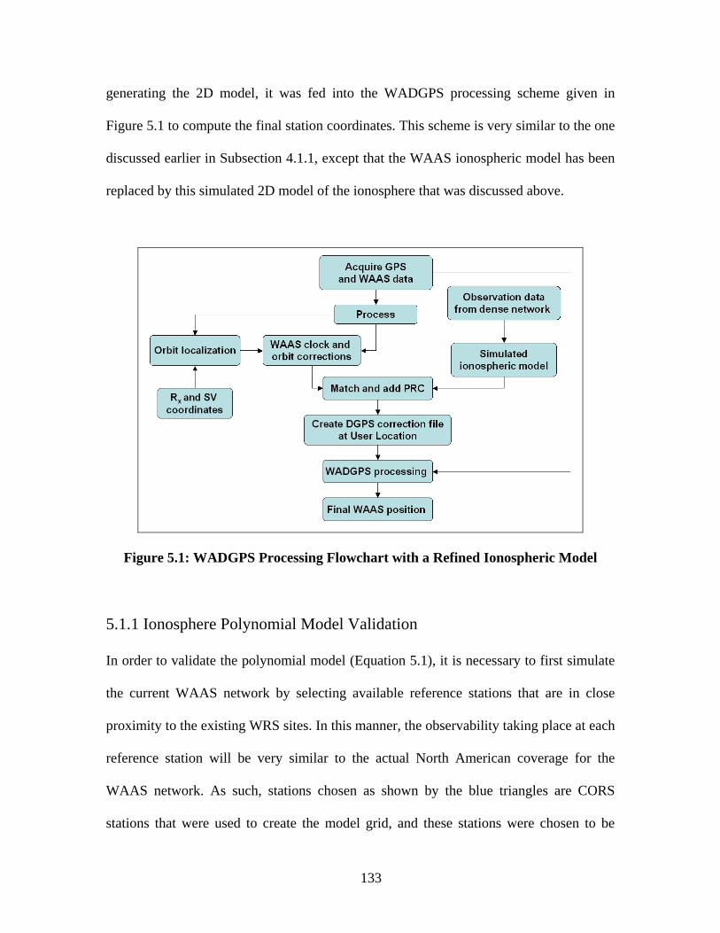
generating the 2D model, it was fed into the WADGPS processing scheme given in
Figure 5.1 to compute the final station coordinates. This scheme is very similar to the one
discussed earlier in Subsection 4.1.1, except that the WAAS ionospheric model has been
replaced by this simulated 2D model of the ionosphere that was discussed above.
Figure 5.1: WADGPS Processing Flowchart with a Refined Ionospheric Model
5.1.1 Ionosphere Polynomial Model Validation
In order to validate the polynomial model (Equation 5.1), it is necessary to first simulate
the current WAAS network by selecting available reference stations that are in close
proximity to the existing WRS sites. In this manner, the observability taking place at each
reference station will be very similar to the actual North American coverage for the
WAAS network. As such, stations chosen as shown by the blue triangles are CORS
stations that were used to create the model grid, and these stations were chosen to be
133
really close (less than 300 km) to the current WRSs so that spatial consistency is
maintained, as shown in Figure 5.2. The average distance between the CORS simulation
stations and corresponding WRSs is 55.4 km. This validation serves the purpose of
showing that the polynomial model simulating the WAAS network is an adequate
approximation of the WAAS model. This is why only the WRS model stations were
shown below, and later when the enhanced network will be presented, more stations will
be simulated, thus fully modelling a denser WAAS network. Consistency would not be
preserved if data from actual WAAS WRSs were to be used because then the dense
network would include both WAAS WRSs and CORS simulated stations, which would
produce biases or systematic errors due to having data from entirely two different
networks. This is why actual WAAS WRSs were not used in the simulation. Another
point to be noted is the fact that WAAS Alaskan stations were not included in the
simulation. This was done for the sake of simplicity/clarity (core network
simulation/densification is the focus here), and it was found that those stations up in
Alaska have very minimal affect on the WAAS network located in the CONUS region.
134

-130 -120 -110 -100 -90 -8025
30
35
40
45
50
Longitude (deg)
Latit
ude
(deg
)
Figure 5.2: Existing WAAS WRS (Red) versus Simulated (Blue) WAAS Network
The validation of the constructed ionosphere model was twofold: 1) observe the
difference in vertical ionospheric delay (expressed in VTEC) between WAAS and
simulated model predictions at standard IGPs during ionospherically quiet time and 2)
observe this vertical ionospheric delay during ionospherically disturbed time. Figure 5.3a
and 5.3b respectively show the results of this analysis. The intent here is to show that the
modelling technique used to simulate the generation of a WAAS ionospheric correction
grid (Equation 5.1) for North America is consistent with the existing WAAS model
implemented by the FAA. Improvements in ionosphere modeling can then be
investigated for the addition of CWAAS stations or densification of the full North
American WAAS network. It is intended that very minimal modelling errors should be
introduced with the method implemented here, and that almost all of the noticeable
135

changes in positioning accuracy and ionosphere corrections are due to adding more
reference stations to the WAAS network.
As can be seen from Figure 5.3a (average ionospheric condition was seen during this
time period, as discussed in Chapter 3), across North America the difference in VTEC is
less than half a metre. These plots were generated by computing the RMSE of the vertical
delay during the given time-period for each of the two networks (Existing WAAS WRS
versus Simulated WAAS Network) shown in Figure 5.2 and then taking the difference. It
would be useful to also show the absolute plots for comparison of the two methods.
Figure 5.3b (disturbed ionospheric condition was seen during this time period, as
discussed in Chapter 3) shows the errors to be slightly higher than the former, still even
during peak storm time the modelling errors are less than 0.5 m. Furthermore, Figure 5.4
is demonstrating that over time VTEC errors (at a single site – its location is shown by a
black circle in Figure 5.3a) are consistently within the half-metre error bound. This plot
was generated by computing the vertical delay at the given station during the October
2003 storm for each of the two networks (Existing WAAS WRS versus Simulated
WAAS Network) shown in Figure 5.2 and then taking the difference. Therefore, it is safe
to assume that the polynomial model errors are minimal and that any improvements
observed from this simulation are very close to those expected from CWAAS or other
enhancements to the WAAS network.
136

Figure 5.3a: Difference between VTEC Figure 5.3b: Difference between VTEC
for WAAS Ionosphere Model versus the for WAAS Ionosphere Model versus the
Polynomial Model at Standard IGPs Polynomial Model at Standard IGPs
(0600-0630 UT, October 30, 2003) (2100-2130 UT, October 30, 2003)
Figure 5.4: VTEC Difference between Existing and Simulated WAAS during the
October 2003 Storm Event at Station "AMC2" for all Satellites in View
5.2 CWAAS Configuration Analysis
137

The discussion in this section involves studying the effects of adding the proposed
CWAAS reference stations. In particular, a better-sampled ionosphere model is computed,
one in which additional Canadian reference stations are used to derive the ionosphere
estimates at WAAS IGPs. Positioning accuracies are then computed using this new
model, as opposed to the current WAAS ionosphere model. WAAS clock and orbit
corrections remain unchanged. Before reporting any results for this section, it will be
shown that the ionosphere modelling technique used to simulate the proposed CWAAS
configuration and grid interpolation is consistent with the WAAS current model. This
will be accomplished by demonstrating that very minimal error exists due to the
inadequacy of this simulated WAAS model. Once this is established, it is possible to
spatially simulate the WAAS and/or CWAAS networks using CORS stations in the
vicinity of existing and proposed WAAS WRSs. First, the November 2003 storm event
will be used to observe how having the proposed CWAAS stations in Eastern Canada
would strengthen the WAAS ionosphere model. A simulated “user” station located at the
centre of the CWAAS network will be used to study the improvements during intense
ionospheric activity. The last element of study in this regard will be to observe the
improvements spatially and if the additional CWAAS stations would have any positive
impact on performance in the west, especially during geomagnetic storm situations.
5.2.1 CWAAS Evaluation in Eastern Canada
138

The model network used for this purpose is given in Figure 5.5 and shows all the model
stations used to simulate CWAAS and overlaid on top are the actual WAAS WRS
locations and proposed CWAAS reference stations (refer to station locations given in
Chapter 2 discussion of CWAAS). This is to show that the model stations were selected
on the basis that spatially it resembles the WAAS + CWAAS network in Eastern Canada
scheduled to be completed in 2006. The CORS site “VALD” (latitude: 48.80971° and
latitude: -77.5642°), located in Val D’Or, Quebec, was chosen to be the “user” test station
because its location would have the optimum effect from the proposed CWAAS network
because it is at the centre of this network.
Figure 5.5: Model Network for CWAAS Assessment in Eastern Canada
139

Using this model network, it is possible to spatially model the ionospheric behaviour over
time. An important difference between this model network and the current WAAS
network is the fact that WAAS does not have existing WRSs in Eastern Canada, and so it
has to apply a mathematical extrapolation; the simulation will enable the inclusion of
observations from actual reference stations into the ionosphere model. The November
2003 storm event was used for these testing purposes, since a phenomenon of interest
occurred in Eastern Canada during this event (see Chapter 3). Figure 5.6 presents the
results obtained as a time-series plot during this event for the following four different
methods (the numbers in the brackets in Figure 5.6 refer to the four positioning modes
below):
1) Single Point
This is the most basic method of GPS positioning. It involves simply taking the raw L1
pseudorange observations and computing the best estimated solution. Standard
atmospheric models were applied: the broadcast model for the ionosphere and the
Hopfield model for the troposphere [Hopfield, 1969]. Additionally, no carrier phase
smoothing was applied during processing.
2) WADGPS using Current WAAS Corrections
This is a WADGPS method that augments the single point solution in terms of accuracy
with (existing current) WAAS provided corrections for clock, orbit and ionosphere. In
theory, this solution should be better than single point. The ionospheric model was
obtained from the WAAS grid, and the tropospheric model used was Hopfield.
140

3) WADGPS using Simulated WAAS Network
Basically this is the same as the method 2, except that the WAAS ionospheric model was
replaced by the Simulated WAAS ionospheric model using reference stations
approximating the current WRS configuration (red triangles in Figure 5.5). The WAAS
clock and orbit corrections are used.
4) WADGPS using Simulated CWAAS Network
This is again similar to method 2, but this time the ionospheric model was generated from
the Simulated CWAAS model network (yellow triangles in Figure 5.5). The WAAS
clock and orbit correction sets are used.
Note: For all four methods the processing was done using a mask angle of 10°; HDOP
filter was set to 2.3 and PDOP at 3.0.
141

0 5 10 15 200
10
20
30
40
95th
-per
cent
ile H
A (m
)
Hours (UT)
Horizontal and Vertical Accuracies on November 20, 2003 at Station "VALD"
0 5 10 15 200
10
20
30
40
95th
-per
cent
ile V
A (m
)
Hours (UT)
Single Point (1)Current WAAS (2)Simulated WAAS (3)Simulated CWAAS (4)
Single Point (1)Current WAAS (2)Simulated WAAS (3)Simulated CWAAS (4)
Figure 5.6: WAAS HA and VA on November 20, 2003 at Station "VALD"
Thus, a second purpose exists in showing this plot; that is to compare the different
methods and observe how the current WAAS compares to the simulated WAAS in the
positioning domain. Recall that the Simulated WAAS was devised by taking ionospheric
truth observations from CORS stations and applying a 2D cubic function to interpolate
the data at standard grid points. On the other hand, the current WAAS model entails
using all observation data surrounding the WRS and applying a planar fit at every IGP to
compute an ionospheric delay estimate.
142

The first comment to be made is about the sharp increase in error (for both HA and VA)
around 2000 UT for all four methods. This sudden degradation in accuracy is due to SED
because similar peaks were seen in time series plots for ionospheric delay at around the
same time, and it has also been shown in numerous spatial plots earlier in Chapter 3.
Typically the accuracies are better than 5 m (at the 95th-percentile), but SED causes the
errors to increase to over 30 m in some cases. A summary of the statistics for this dataset
is provided in Table 5.1. The statistics were separated into quiet and active ionospheric
times to observe the level of degradation in positioning accuracy once the storm
commenced. In general the RMSE went up about 100% during the disturbed periods.
Table 5.1: Overall HA and VA Positioning Statistics on November 20, 2003 at
Station VALD for Quiet (0000-2000 UT) and Active (2000-2400 UT) Ionosphere
Single Point Current WAAS Simulated WAAS
Simulated CWAAS
Quiet Active Quiet Active Quiet Active Quiet ActiveMEAN 2.53 5.34 1.29 4.32 1.43 4.41 1.02 3.12 RMS 3.12 6.09 2.87 5.96 3.02 6.31 1.34 2.49 STD 2.91 5.68 2.48 5.79 2.68 6.02 0.89 2.16 95% 6.79 12.49 7.87 10.92 7.92 11.06 2.24 6.31 MAX 5.13 30.46 4.96 23.75 5.23 24.32 4.98 10.42
HA
(m)
MIN 0.13 7.87 0.03 5.35 0.07 5.74 0.03 2.56 MEAN 3.46 6.45 3.12 5.64 3.42 5.75 1.56 2.89 RMS 4.12 7.29 3.98 6.73 4.06 6.84 1.67 3.45 STD 3.65 6.83 3.42 6.24 3.63 6.44 1.23 3.11 95% 7.56 14.25 6.45 13.12 6.70 13.56 2.86 7.49 MAX 6.23 54.63 5.87 26.61 5.96 28.01 5.23 12.07
VA
(m)
MIN 0.32 11.54 0.06 7.23 0.11 7.53 0.13 2.89
143

In terms of comparing between the methods, the most interesting point about this plot is
how single point performs better horizontally than WAAS during 2000-2200 UT. One
possible explanation for this is that since WAAS has no WRSs in Eastern Canada (thus
no actual observations from there are input for the WAAS model), coverage is so
minimal and only extrapolated model is available over that region, WAAS model is not
as accurate as broadcast model for single point. This is especially the case during intense
ionospheric times, but in general WAAS performs better than single point since typical
accuracies (during ionospherically quiet times) are greater. The notion could be further
investigated with the aid of ionospheric correction data. Thus, plots were generated
showing the ionospheric delay accuracies for WAAS versus Broadcast (Figure 5.7). In
both cases the vertical delays are being underestimated, and the differenced values are
mostly negative. During the ionospherically quieter times, WAAS values are more
accurate but during intense times the Broadcast delay values are closer to truth. This is
sort of the scenario that was seen in the positioning plots above, where single point was
doing more accurate WAAS during 2000-2200 UT.
144

Figure 5.7: VTEC WAAS vs. Broadcast Accuracy on November 20, 2003 at Station
"VALD"
Nonetheless, it is noticeable that the two variants of WAAS (simulated versus existing)
are very similar in the positioning domain, which is indicative of the fact that the 2D
interpolation used to simulate the WAAS ionosphere model is valid. This was also shown
earlier in Subsection 5.1.1 using a VTEC-difference spatial map but in the correction
domain.
Finally, simulated CWAAS has performed better than the other methods; this is mainly
because in this case actual observations in the vicinity of “VALD” went into the model.
In the other cases (current and simulated WAAS – methods 2 and 3), only a mathematical
145

extrapolation is used to spatially model that area in terms of ionosphere, and therefore
does not adequately capture the true physical phenomenon.
5.2.2 WAAS/CWAAS Evaluation in North America
A broader model network was devised to assess the full WAAS/CWAAS station
configuration. It included CORS stations that were near the existing WAAS reference
stations and those that were near the proposed CWAAS stations. This model network is
shown in Figure 5.8. This is what the full WAAS/CWAAS would look like in 2006 when
all of the CWAAS stations would have been deployed. Previously, it was shown that
CWAAS would offer better performance for the ionosphere model in Eastern Canada, but
it would also be interesting to see if there are any benefits in other regions as a result of
having the new sites in the east. Accordingly, the main intention in simulating this
scenario is to observe the positive impact (if any) of CWAAS in Western Canada during
ionospheric storm events.
146

Figure 5.8: Full Configuration of WAAS + CWAAS Model Network Using the truth data from the above network and applying a 2D cubic fit across North
America, the ionospheric model for a given epoch was created. Even though the WAAS
uses a local bi-linear fit at each IGP and a global 2D cubit fit is used here, the modelling
errors due the dissimilar fits are insignificant, as was shown in Subsention 5.1.1. The
following positioning spatial maps present the 95th-percentile positioning accuracies
during 2200-2230 UT on October 30, 2003. As will be seen later in the time series plots,
during this time-interval major error peaks were seen. The horizontal, vertical and 3D
accuracies are respectively given by Figures 5.9, 5.10 and 5.11.
Clearly, CWAAS is not improving the horizontal positioning performance in Western
Canada; the errors remained constant even after adding the additional reference stations.
By observing the vertical and 3D errors, it could be said that slight degradation in
147

accuracy occurs after adding the CWAAS reference stations. It should not be assumed
that the additional stations are having a negative impact on vertical accuracy. Rather, it is
suspected that the slight degradation is caused by modelling errors that were discussed
earlier and shown in Figures 5.3a, 5.3b and 5.4. Hence, if the modelling technique
employed here and the one used by WAAS were exactly the same, there would be no
degradation, as in the horizontal case; this discrepancy is only apparent in the vertical
because height determination is more sensitive to ionosphere modelling errors than the
horizontal components. In general, CWAAS would not improve performance for users in
Western and central Canada. Thus, CWAAS development should include some reference
stations in the west as well, to allow wide-area positioning benefits across Canada.
Figure 5.9: WAAS vs. WAAS + CWAAS Horizontal Positioning Accuracies (2200-
2230 UT, October 30, 2003)
148

Figure 5.10: WAAS vs. WAAS + CWAAS Vertical Positioning Accuracies (2200-
2230 UT, October 30, 2003)
Figure 5.11: WAAS vs. WAAS + CWAAS 3D Positioning Accuracies (2200-2230 UT,
October 30, 2003)
149

5.3 Assessment of the Enhanced WAAS
This final set of results will entail studying a hypothetical network that will model the
ionosphere using more than 50 reference stations (Figure 5.12). It is to be noted that this
network will include simulated WAAS and CWAAS stations (to approximately simulate
the expected 2006 CWAAS infrastructure) as well as additional evenly distributed CORS
stations to increase the station density throughout North America. The selection of the
simulated stations was primarily based on proper spatial coverage and even distribution
of sites throughout the network. However, it wasn’t always possible to maintain these
criteria because sometimes full datasets weren’t available for the desired stations and
time period; thus, the densified network couldn’t be optimally distributed and some areas
of the network possess uneven coverage.
The standard WAAS ionospheric model will be replaced by the polynomial ionosphere
model (Equation 5.1) that was simulated using a denser network, similar to that computed
in the previous section, and the clock/orbital error models will remain the same in the
WAAS correction domain. The intent is to show how this refined ionospheric model
would drastically improve WAAS performance in terms of accuracy due to its denser
sample of the true physical process of the ionosphere. Thus, the so-called Enhanced
WAAS will be put to the test during one of the storm events discussed throughout this
research. This scenario is rather close to reality as future densification of the WAAS
network is on the horizon and is being planned by the FAA and Raytheon. The current
phase of the WAAS would incorporate four new stations in Alaska, four in Canada
150

(CWAAS), and five in Mexico. As well, additional reference stations may be included in
the core CONUS region but this is not definite, and so the details have not been disclosed
yet [Cormier, 2005].
-130 -120 -110 -100 -90 -80 -70 -6025
30
35
40
45
50
55
60
Longitude (deg)
Latit
ude
(deg
)
Figure 5.12: Enhanced WAAS Model Network Using 50+ Reference Stations (Blue
Triangles are Stations Modelling Existing WAAS WRSs and Red Triangles are
Additional Model Stations to Densify the Network and includes CWAAS RSs)
5.3.1 Observability Improvements for the Enhanced WAAS Network
An important aspect to investigate is the observability improvements to be gained via this
densification. As such, a partial (for the sake of simplicity and clarity in the plots) area of
this network in North America was chosen to study the increase in observability. Shown
below in Figure 5.13 are five stations near the Great Lakes that are part of this Enhanced
WAAS network. The four blue triangles represent the additional stations added to the
151

simulated network to further increase density and the red signifies a station that is
approximating the location of one of the existing WAAS WRSs. The intent here is to
provide an example of the observable redundancy that could be gained if WAAS were to
possess more reference stations across North America.
Figure 5.13: Partial Enhanced WAAS Network near the Great Lakes
One way to study measurement redundancy is to look at the IPPs for each station. And so,
two plots were created: 1) the IPPs for the single WAAS WRS in the area are plotted
(Figure 5.14) and 2) the IPPs for all five WRSs in the area are plotted (Figure 5.15). Note
that the gridline intersections in these plots represent WAAS IGPs (5° x 5°). Clearly, the
redundancy would increase by a factor of five (give or take a few coincident IPPs), and
visually the second plot shows significantly more satellite observations than the first.
Thus, it is easily conceivable that for the full network configurations significant
observability improvements would exist. However, performance improvements are not
solely dependent on network density. There is another aspect to obtaining benefits in the
152

positioning domain and that is the spacing of the IGPs. This issue will be further
discussed later in the chapter.
Figure 5.14: Single Station IPP Distribution Plot
Figure 5.15: Multiple Station IPP Distribution Plot
153

A spatial analysis, similar to the ones in earlier sections, of the Enhanced WAAS will be
conducted first. The analysis involves comparing the 95th-percentile horizontal (Figure
5.16) and vertical (Figure 5.17) accuracies of the current WAAS against the Enhanced
WAAS. This analysis was done by first creating model of the ionosphere for the given
days using the polynomial model and ionospheric truth data as inputs. This provided an
ionospheric grid (5˚ x 5˚) similar to that of WAAS, except that this model was defined by
many more observations (due to higher number of reference stations). Then at user “test”
stations, both WAAS and Enhanced WAAS positioning were conducted. Figure 5.18
shows a map of the user “test” sites overlaid on top of the simulated reference stations.
There is independence between the user “test” stations and the model stations, but
sometimes the “test” stations had to be located fairy close to model stations because
either data weren’t available (data missing on archived web server) or better candidate
stations did not exist. Nonetheless, in general the two sets of stations are reasonably
spaced apart to provide independent solutions. As shown in the above two plots, the
observability would improve significantly for the denser network, thus increasing
redundancy and in turn strengthening the positioning solution. It wouldn’t be practical to
show the observability of the (full) dense network because the satellite traces would be so
dense that the curves would overlap and no patterns would be visible. This is why only a
portion of the network observability was presented to observe the improvements.
154

Figure 5.16: WAAS vs. Enhanced WAAS Horizontal Positioing Accuracies (2300-
2330 UT, October 30, 2003)
X
Figure 5.17: WAAS vs. Enhanced WAAS Vertical Positioing Accuracies (2300-2330
UT, October 30, 2003)
155

Figure 5.18: Map of User “Test” Sites (magenta triangles) Overlaid on top of the
Simulated Reference Stations
Both in the horizontal and in the vertical, Enhanced WAAS offered much better
performance levels as compared to current WAAS. For instance, at five stations the HA
exceeds 15 m for current WAAS but this is true at only one station for the latter; also, the
overall positioning errors are significantly reduced using the refined model of the
ionosphere. Furthermore, maximum VA for current WAAS is about 23 m but its
counterpart provided errors not exceeding 17 m across North America.
156

After this spatial analysis, it is interesting to study the benefits temporally. As such, a
station (“AZCN” shown by a black cross Figure 5.17 and a black circle in Figure 5.18)
was chosen directly beneath the SED. Once again the accuracies are plotted as a time
series for this single station, over three days (the full October 2003 storm event).
Accuracy plots of other time intervals for this event can be found in Appendix D.
Figure 5.19 shows the 95th-percentile HA and VA for single point, current WAAS and
Enhanced WAAS over time during October 29-31, 2003. These plots are generated by
computing the 95th-percentile over half hour periods for each of the three methods and
representing them at the centres of those half hours. This helped in removing some of the
noise components in the dataset. Note that for all positioning solutions were computed
using a mask angle of 10°; HDOP filter was set to 2.3 and PDOP at 3.0. The results
presented in the figure below are from a station (“AZCN”, latitude: 36.8398° and
longitude: -109.9251°) that was directly beneath the SED while it traveled through North
America. As can be seen, both vertical and horizontal positioning accuracies (computed
by taking the square root of the sum between errors in northing and easting) were poor
near the end of October 29 and 30 (UT) in all three cases; the accuracy degradation
periods in those instances were over 12 hours in length.
The peaks seen in VTEC plots are also present in the positioning plots, which is
indicative of the fact that ionospheric error is the major driving force behind the
positioning error. Near the end of the first and the second day of this event, the errors
rose to ten times the typical level. As expected, single point would perform the poorest
157

compared to the rest; although, there is one instant (second VA peak) where it performs
better than current WAAS. This irregularity has been explained in Subsection 5.2.1.
Evidently, there is considerable improvement offered by Enhanced WAAS in both the
horizontal and vertical accuracy components (more than 100% improvement during SED).
Refer to Table 5.2 for detailed statistics of these results. In addition, the typical values
(during ionospherically quiet times) are also somewhat lower as compared to the levels
offered by the current WAAS.
Figure 5.19: WAAS HA and VA during October 29-31, 2003 at Station "AZCN"
158

Table 5.2: Overall HA and VA Positioning Statistics for October 2003 Storm Event at Station “AZCN”
Although the ionosphere is better captured, using a network that is twice as dense, these
results may be misleading because the dense network observations are still reduced to a
fixed set of IGP located no closer than 5 degrees apart. In this case it is usually expected
that some spatial resolution to be lost. But the improvements seen herein are significant.
In this context, improvements in the positioning domain depend upon two factors: the
network density and grid spacing. There is a saturation point for improvements gained
due to network densification. In other words, there is a point in the level of densification
where addition of reference stations will cease to affect network performance. On the
other hand, the grid spacing would have no such limit because the discretization would
approach the continual spatial as the spacing between IGPs become infinitesimally small;
this parameter would only be bound by practicality (e.g. computation load, data
management, band width, etc.).
159

For the results obtained herein, it appears that this densification limit has not been
reached since improvements are significant. Perhaps, the level of improvement is an
indication of the fact that optimum balance between network density and spatial
resolution has been reached. Having more reference stations is definitely helping to
obtain more observation points near the IGPs (as shown earlier in IPP distribution plots
show here as well), which is providing more accuracy. But, beyond a certain point IPPs
will not approach IGPs and the measurements still will be reduced to the five-degree IGP
spacing. Further study would be required to determine which densification level is
required for optimal performance by the WAAS network. According to the results
obtained here, decreasing the station spacing in the WAAS network would improve
performance of the system. The level of densification that was studied herein showed
significant improvement, but from this research it is not clear that this is the optimum
level of densification, in that, if at this densification level the lowest cost/benefit ratio is
obtained and if saturation of improvements has occurred or not. For instance, It could
have been possible to test at IGPs for various station configurations and evaluate the
accuracy at a given grid point for the ionospheric model; however these investigations
fell outside the scope of this research, as the focus here was network densification but did
not include reduced grid spacing. Based on the findings of this chapter, the following
recommendations are made:
• WAAS reference network could include more closely–spaced WRSs to better
model the ionosphere.
160

• The proposed CWAAS station locations in eastern Canada allowed significant
performance improvements during a severe ionospheric storm event. Users in
western Canada would not experience any performance improvement from this
CWAAS development, however. As such, the CWAAS reference network would
benefit from additional sites in the west.
• A study should be conducted to investigate the potential improvements that could
be obtained from reducing the WAAS ionospheric grid spacing.
161

Chapter 6
Conclusions and Recommendations
6.1 Conclusions
The main objectives of this research were to evaluate the current WAAS (accuracy)
performance in the correction domain, assess its positioning capabilities across North
America under various ionospheric conditions, and finally to devise a better sampled
ionospheric model using a denser/expanded network to study the potential future
improvements in positioning performance for WAAS/CWAAS across North America,
again under various ionospheric conditions. The major motivation for this was taken from
162

the fact that under the effects of SED, considerable accuracy degradation is experienced
when trying to conduct positioning using a wide-area approach such as WAAS. The
phenomenon is caused by enhanced ionospheric electric fields that are present near the
mid- to high-latitudes during geomagnetically disturbed periods and are characterized by
large TEC gradients, both spatially and temporally. SED causes positioning performance
to deteriorate very rapidly, and even wide-area systems like the WAAS are unable to
fully model the ionospheric behaviour during those times. This is even a bigger problem
in Canada since very minimal WAAS coverage exists and no reference stations are
actually located in Canada. Therefore, investigation of these issues is necessary.
This study has shown that typically WAAS clock and orbital errors are more accurate
than broadcast clocks and orbits, but there could be some infrequent outliers due to
satellites just coming into view or the age of correction being significantly large. Usually,
these satellites are outside of network coverage but there are odd instances when satellites
in view have large correction age. Because this is very infrequent, it has minimal impact
in the positioning domain since it is one bad observation against hundreds of valid ones.
Additionally, it is has been shown that the WAAS UDRE bounds all the errors, and in the
positioning domain the protection levels (HPL and VPL) also bound the positioning
errors; thus WAAS reliability was preserved during the course of the periods studied
herein. In general, WAAS ionospheric corrections tend to be very smooth, and so the
localized features are not captured well. This is due to having only 25 WRSs and 5° x 5°
grid spacing. As it was shown in numerous TEC maps, the SED is a narrow plume of
enhanced total electron content extending northerly through Canada which is not detect
163

by WAAS for the most part. This is of major concern for a user trying to position using
WAAS when they are directly beneath the SED phenomenon, since the vertical
ionospheric delay errors sometimes exceeded 15 m. It is not difficult to estimate the
negative impact this will have in the positioning domain, but WAAS reliability was
maintained in all instances by having the GIVE values bound the VTEC errors. As well,
WAAS has proven to be at least much better than the broadcast (Klobuchar) model, in
terms of accuracy of the ionospheric delay.
In the positioning domain, typical WAAS horizontal accuracies were well below the
threshold levels set by regulating bodies for marine or land navigation, but during storm
periods of SED WAAS accuracies degraded severely and far surpassed those safety
thresholds (10 m HA at the 95th-percentile). Since WAAS is a system that provides
vertical guidance to aircrafts, it was essential to closely observe the height estimation. As
is the case in any satellite-based navigation system, the vertical component is the hardest
of the three to estimate. As such, it was seen that vertical errors were much more
significant than the horizontal ones, and it raised the 3D errors to very high levels.
Although the errors were large, the GIVE values provided the reliability necessary to
offer adequate service, but during some storm events the vertical service was denied for
all users in North America due to “unmonitored” GIVE predictions.
The study of the refined ionospheric model had two components to it: 1) to test the
CWAAS candidate sites and 2) to assess the improvements of having a denser network of
reference stations. For the CWAAS assessment, it was found that the proposed sites
164

would greatly aid in improving WAAS performance in Eastern Canada, but the benefits
of CWAAS was virtually non-existent in Western Canada. As for the Enhanced WAAS,
it was shown that if the WAAS were to have more than 50 stations in its network, the
positioning errors would be reduced by a factor of two during SED and the typical error
levels would also decrease.
The research led to conclusions about where challenges for WAAS exist and how it
would be possible to strengthen those areas of the system. The major contributions of this
research are:
• Identification of WAAS error behaviours for clock, orbit and ionosphere
• Comparison of WAAS corrections with those provided by broadcast
• Performance analysis of the WAAS in terms of accuracy, reliability and
coverage in both spatial and temporal domains
• Quantification of positioning accuracies from different perspectives and
various ionospheric conditions
• Simulation of WAAS/CWAAS networks to assess the validity of the proposed
station locations and density
• Evaluation of the Enhanced WAAS in the positioning domain
165

6.2 Recommendations
The major problem with clock/orbital corrections has been the presence of outliers, which
could cause positioning inabilities. Therefore, WAAS-enabled receivers should have a
filtering mechanism to reject any observation that is deemed to be an outlier. As
discussed earlier, a strong correlation exists between these outliers and when the satellite
came into view and/or the age of correction, and there are instances when old corrections
are available for satellites in view. Thus, the filtering method could be based on these two
criteria in conjunction with the sheer magnitude of the outlier.
CWAAS evaluation was done to investigate if the candidate sites are optimal from
positioning and practical perspectives; its benefits, however, were only seen in the east.
Therefore, CWAAS development should also include a few reference stations in Western
Canada, where the coverage is minimal and where the stations would best complement
the existing WRSs.
The Enhanced WAAS has been shown to offer a great deal of benefits in all respects of
positioning. Consequently, the FAA should consider adding more reference stations also
to the core WAAS network, and there are talks that further development of the WAAS
infrastructure is being envisioned by the FAA. However, adding more stations is just
solving part of the problem; the other part is grid spacing, which will still be very coarse.
One can have a sparse network and fine grid spacing or vice versa but still end up with
poor results because both of these elements have to be appropriately dense or fine. In
166

practice, there are physical limits as to how dense a network or how fine the grid spacing
could or should be. For instance, after a certain point no matter how many stations are
added the accuracy will not improve further because the users will not necessarily be
close enough to a given IGP. Nonetheless, in the results obtained here it has been shown
that the model is definitely improved when more stations are added to the reference
network. Thus, the method of improving the level of service would be also to lower the
grid spacing, but this will entail reworking the message structure and upgrading to high
bandwidth transmitters throughout the system – which is not likely. Thus, it becomes a
question of cost versus benefit. Nonetheless, the options are there for future
enhancements to the WAAS – it is a matter of implementing them if the feasibility exists.
In addition to SBAS, which was the focus of this research, nowadays other augmentation
methods are being used to supplement GPS accuracy, reliability, integrity, continuity and
availability. These include other GNSS, ground-based augmentations, pseudolites, GPS
occultations, etc [Shively, 2004]. In addition to what was discussed in this study, the FAA
should look into integrating some of these methods of positioning to further enhance
WAAS services offered to its users. When making a modification of this scale, the main
concern is reliability. If the additional supports could offer similar of higher levels of
reliability at reasonable costs, then the integration would add value to the system in the
long run.
167

Appendix A
Ionospheric TEC Plots on October 29, 2003
A1: Truth VTEC Map (1900- A2: WAAS VTEC Map (1900-
1930 UT, October 29, 2003) 1930 UT, October 29, 2003)
168

A3: Truth VTEC Map (2000- A4: WAAS VTEC Map (2000-
2030 UT, October 29, 2003) 2030 UT, October 29, 2003)
A5: Truth VTEC Map (2100- A6: WAAS VTEC Map (2100-
2130 UT, October 29, 2003) 2130 UT, October 29, 2003)
169

A7: Truth VTEC Map (2200- A8: WAAS VTEC Map (2200-
2230 UT, October 29, 2003) 2230 UT, October 29, 2003)
Ionospheric TEC Plots on October 30, 2003
A9: Truth VTEC Map (1900- A10: WAAS VTEC Map (1900-
1930 UT, October 30, 2003) 1930 UT, October 30, 2003)
170

A11: Truth VTEC Map (2000- A12: WAAS VTEC Map (2000-
2030 UT, October 30, 2003) 2030 UT, October 30, 2003)
A13: Truth VTEC Map (2100- A14: WAAS VTEC Map (2100-
2130 UT, October 30, 2003) 2130 UT, October 30, 2003)
171

A15: Truth VTEC Map (2200- A16: WAAS VTEC Map (2200-
2230 UT, October 30, 2003) 2230 UT, October 30, 2003)
172

Appendix B
Ionospheric TEC Accuracy Plots on
November 20, 2003
B1: Truth VTEC Map (1800- B2: WAAS VTEC Map (1800-
1830 UT, November 20, 2003) 1830 UT, November 20, 2003)
173

B3: Truth VTEC Map (1900- B4: WAAS VTEC Map (1900-
1930 UT, November 20, 2003) 1930 UT, November 20, 2003)
B5: Truth VTEC Map (2000- B6: WAAS VTEC Map (2000-
2030 UT, November 20, 2003) 2030 UT, November 20, 2003)
174

B7: Truth VTEC Map (2100- B8: WAAS VTEC Map (2100-
2130 UT, November 20, 2003) 2130 UT, November 20, 2003)
175

Appendix C
Positioning Accuracy Plots for Current
WAAS on October 30, 2003
C1: WAAS Horizontal Accuracies C2: WAAS Vertical Accuracies
(1900-1930 UT, October 30, 2003) (1900-1930 UT, October 30, 2003)
176

C3: WAAS Horizontal Accuracies C4: WAAS Vertical Accuracies
(2000-2030 UT, October 30, 2003) (2000-2030 UT, October 30, 2003)
C5: WAAS Horizontal Accuracies C6: WAAS Vertical Accuracies
(2100-2130 UT, October 30, 2003) (2100-2130 UT, October 30, 2003)
177

C7: WAAS Horizontal Accuracies C8: WAAS Vertical Accuracies
(2200-2230 UT, October 30, 2003) (2200-2230 UT, October 30, 2003)
178

Appendix D
Positioning Accuracy Plots for Enhanced
WAAS on October 30, 2003
D1: EWAAS Horizontal Accuracies D2: EWAAS Vertical Accuracies
(2000-2030 UT, October 30, 2003) (2000-2030 UT, October 30, 2003)
179

D3: EWAAS Horizontal Accuracies D4: EWAAS Vertical Accuracies
(2100-2130 UT, October 30, 2003) (2100-2130 UT, October 30, 2003)
D5: EWAAS Horizontal Accuracies D6: EWAAS Vertical Accuracies
(2200-2230 UT, October 30, 2003) (2200-2230 UT, October 30, 2003)
180

D7: EWAAS Horizontal Accuracies D8: EWAAS Vertical Accuracies (2300-2330 UT, October 30, 2003) (2300-2330 UT, October 30, 2003)
181

References
Altshuler, E., D. Cormier and H. Go, Improvements to the WAAS ionospheric algorithms,
Proceedings of the ION GPS 2002, Sept. 24-27, Portland, OR, pp. 2256-2261, 2002.
Bunce, D., Wide Area Augmentation System, Presentation Slides, WAAS Product Team,
Federal Aviation Administration (FAA), July 2003.
Cannon, M.E. and Lachapelle, G., Analysis of a High-Performance C/A-Code GPS
Receiver in Kinematic Mode”, NAVIGATION: The Journal of the Institute of Navigation,
Vol. 39, No. 3, Fall 1992, http://www.novatel.ca/Documents/Papers/File3.pdf.
Cannon, M.E., G. Lachapelle and W. Qui, C3NAVTM Operating Manual Version 2.0, The
University of Calgary, Calgary, Alberta, 1995.
Cannon, M.E., Skone, S., Gao, Y., Moon, Y., Chen, K., Crawford, S. and G. Lachapelle,
“Performance Evaluation of Several Wide-Area GPS Services”, Conference Proceedings
of ION GPS-02, Portland, September 24-27, 2002.
Conley, R., “Results of the GPS JOP’s GPS Performance Baseline Analysis: The Gospar
Project”, NAVIGATION: The Journal of the Institute of Navigation, Vol. 45, No. 1, 1998.
182

Continuously Operating Reference Stations (CORS),
http://www.ngs.noaa.gov/CORS/cors-data.html, January 2005.
Cormier, D., McKendree, T.L., Schempp, T.R., “Concept for New SBAS Message Types
to Improve GIVE Resolution”, ION NTM 2005, 24-26 January 2005, San Diego, CA.
Coster, A. J., J. C. Foster and P. J. Erickson, Monitoring the ionosphere with GPS, GPS
World, pp. 40-45, May 2003.
Coster, A. J., J. C. Foster, P. Erickson, B. Sandel and F. Rich, Monitoring space weather
with GPS mapping techniques, Proceedings of the ION National Technical Meeting 2003,
Anaheim, CA, January 22-24, 2003.
Dai, D., Walter, T., Enge, P. and Powell, J.D., “Optimal Use of Ionospheric Corrections
for Wide Area Augmentation System (WAAS) Users”, Stanford University, IEEE,
Volume 0-7803-4330-1/98, 1998.
El-Arini, M.B., Conker, R., Albertson, T., Reegan, J.K., Klobuchar, J.A., and Doherty, P.,
“Comparison of real-time ionospheric algorithms for a GPS wide-area augmentation
system (WAAS)”, NAVIGATION: Journal of the Institute of Navigation, vol. 41, no. 4,
pp. 393-413, winter 1994-95.
183

El-Arini, M.B. and Lejeune, R.O., “Description of an Ionospheric Spatial Gradient
Irregularity Detectors for WAAS” The MITRE Corporation, Center for Advanced
Aviation System Development (CAASD) (Journal), 2001.
Enge, P.K. and Van Dierendonck, A.J., “Wide Area Augmentation System”, Chapter 4 of
Global Positioning System: Theory and Applications Volume II, American Institute of
Aeronautics and Astronautics, Inc., Washington, DC, 1996.
Farah, F., “The Ionospheric Delay Effort for GPS Single-Frequency Users-Analysis
Study for Simulation Purposes”, The University of Nottingham, UK, August 2001.
Federal Aviation Administration (FAA), GPS Basics,
http://gps.faa.gov/gpsbasics/index.htm, December 2004.
Federal Aviation Administration (FAA),
http://gps.faa.gov/Programs/WAAS/waas.htm, February 2005.
Foster, J. C., P. J. Erickson, A. J. Coster, J. Goldstein and F. J. Rich, Ionospheric
signatures of plasmaspheric tails, Geophys. Res. Lett., 29(13), 10.1029/2002GL015067,
2002.
184

Foster, J.C. and H. B. Vo, Average characteristics and activity dependence of the
subauroral polarization stream, Journal of Geophysical Research, 0.1029/2002JA009409,
2002.
Hanlon, D. and K. Sandhoo, (1997) “FAA Satellite Navigation Program Overview”,
Proceedings of the ION Annual Meeting, The Institute of Navigation, Alexandria, VA.,
pp. 49-56.
Hopfield, H.S., “Two-quartic tropospheric refractivity profile for correction satellite
data”, Journal of Geophysical Research, 74, no. 18, 4487, 1969.
Hu, Z., Ning, L., Wang, Y. Li, C. and Yu, J., “The Quality of Service Evaluation Tool for
WAAS”, College of Electronic Science and Technology of China, University of
Electronic Science and Technology of China, IEEE, (Journal) Volume 0-7803-7547-5/02,
2002.
International Reference Ionosphere (IRI),
http://nssdc.gsfc.nasa.gov/space/model/models/iri.html, November 2003.
Jet Propulsion Laboratory (JPL), http://igscb.jpl.nasa.gov/, January 2005.
Kaplan, E.D., Understanding GPS Principles and Applications, Artec House, Norwood,
Massachusetts, 1996.
185

Klobuchar, A.J., Doherty, P.H., El-Arini, M.B., “Potential Ionospheric Limitations to
GPS Wide-Area Augmentation System (WAAS), NAVIGATION: The Journal of the
Institute of Navigation, Vol. 42, No. 2, 1995.
Knight, M., M. Cervera and A. Finn, A comparison of predicted and measured GPS
performance in an ionospheric scintillation environment, Proceedings of the ION GPS-99,
September 14-17, Nashville, Tennessee, 1437-1450, 1999.
Komjathy, A., Sparks, L., Mannucci, A.J. and Pi, X., “An Assessment of the Current
WAAS Ionospheric Correction Algorithm in the South American Region”,
NAVIGATION: Journal of The Institute of Navigation, Vol. 50, No. 3, Fall 2003.
Komjathy, A., Sparks, L., Mannucci, A.J. and Pi, X., “On the Ionospheric Impact of
Recent Storm Events on Satellite-Based Augmentation Systems in Middle and Low-
Latitude Sectors”, Conference Proceedings of ION GPS/GNSS 2003, 9-12 September
2003, Portland, OR.
Krankowski, A., Sergeenko, N.P., Baran, L.W., Shagimuratov, I.I., Rogova, M.V. “The
Short-Term Forecasting of the Total Electron Content” Artificial Satellites, Vol.40, No.2,
2005.
Lachapelle, G., “ENGO 625 NAVSTAR GPS: Theory and Applications”, Department of
Geomatics Engineering, University of Calgary, September 2003.
186

Liu, Z. and Gao, Y., “Development and evaluation of a 3-D Ionospheric Modeling
Method”, NAVIGATION: Journal of The Institute of Navigation Vol. 51, No. 4, Winter
2004.
Loh, R., Wullschileger, V., Elrod, B., Lage, M. and Haas, F., “The U.S. Wide-Area
Augmentation System (WAAS)”, NAVIGATION: Journal of The Institute of Navigation
Vol. 42, No. 3, Fall 1995.
McCaskill, T., Buisson, J. and Buonaguro, A., “A Sequential Range Navigation
Algorithm of Projected DGPS for High-Accuracy DGPS-Based System”,
NAVIGATION: Journal of The Institute of Navigation Vol. 23, No. 2, 1976.
Misra P. and Enge, P.K., “GPS Measurements and Error Sources”, Chapter 4 of Global
Positioning System: Signals, Measurements, and Performance, Ganga-Jamuna Press,
Lincon, Massachusetts, 2001.
Nationwide Differential Global Positioning System (NDGPS),
http://www.tfhrc.gov/its/ndgps/, July, 2003.
NOAA website http://www.sec.noaa.gov/ftpdir//plots/kp/ , December 2003.
NOAA website http://www.sec.noaa.gov/ftpdir//plots/kp/ , January 2005.
187

NAV CANANDA, http://www.navcanada.ca, January 2005.
Parkinson, B.W. and J.J. Spilker, Global Positioning System: Theory and Applications
Volume I, American Institute of Aeronautics and Astronautics, Washington, D.C.,
1996.
Peterson, E.R., Walter, T., Hansen, A., Comp, C. and Enge, P., “The Application of a 3-D
Empirical Ionosphere Model to WAAS Simulation”, Department of Aeronautics and
Astronautics, Stanford University, IEEE, (Journal) Volume 0-7803-4330-1/98, 1998.
Pullen, P.S., Chao, Y.C., Enge, P.K. and Parkinson, B.W., ”Effects of Local Ionospheric
Anomalies on Navigation Performance and Integrity using WAAS”, Department of
Aeronautics and Astronautics, Stanford University, IEEE, (Journal) Volume 0-7803-
3085-4/96, 1996.
Rho, H., Langley R. and Kassam, A, “The Canada-Wide Differential GPS Service: Initial
Performance”, Conference Proceedings of ION GPS/GNSS 2003, 9-12 September 2003,
Portland, OR.
Radio Technical Commission for Aviation Services (RTCA) Inc., “Minimum Operational
Performance Standards for Global Positioning System/Wide Area Augmentation System
Airborne Equipement”,DO-229C, 2001.
188

Rodrigues, F.S., Aquino, M. H. O., Danson, A., Moore, T. and Waugh, S., “Statistical
Analysis of GPS Ionospheric Scintillation and Short-Time TEC Variations over Northern
Europe”, NAVIGATION: Journal of The Institute of Navigation Vol. 51, No. 1, Spring
2004.
Shively, C. A. and Hsiao, T. T., “Availability Enhancements for CAT IIIB LAAS”,
NAVIGATION: Journal of The Institute of Navigation Vol. 51, No. 1, Spring 2004.
Skone, S., “TECANALYS Operating Manual”, Department of Geomatics Engineering,
University of Calgary, September 2002.
Skone, S., Coster, A., Hoyle, V. and Laurin, C., “WAAS Availability and Performance at
High Latitudes”, Conference Proceedings of ION GPS/GNSS 2003, 9-12 September
2003, Portland, OR.
SPARG website http://www.shef.ac.uk/~sparc/tutorial.html#3.0, October 2003.
The Canadian Coast Guard (CCG) website http://www.ccg-gcc.gc.ca/dgps/main_e.htm,
June 2005
The GPS Store website http://www.thegpsstore.com/Detail-Furuno-GP32-GPS-WAAS-
receiver.asp, July 2005.
189

Till, R.D., Wanner, W. and Evangelos, J.R., “Wide Area Augmentation System (WAAS)
Test and Evaluation Concepts”, IEEE, (Journal) CH35797-95/0000-0169, 1995.
U.S. Department of Transportation, “FAA Specification: Wide Area Augmentation
System (WAAS)”, FAA-E- 2892B, 1999.
Van Dierendonck, A.J., P. Fenton and T. Ford, “Theory and performance of narrow
correlator spacing in a GPS receiver”, NAVIGATION: The Journal of the Institute of
Navigation, Vol. 39, No. 3, 283, Fall, 1992,
http://www.novatel.ca/Documents/Papers/File2.pdf.
Walter, T., Course 730: Wide Area Augmentation System (WAAS), ION GPS-2003
Tutorial, Navtech Seminars & GPS Supply, Inc., Alexendria, VA, 2003.
Yousuf, R., Skone, S. and Coster, A., “Evaluation of DGPS and WADGPS Methods for
Land and Marine Applications”, Conference Proceedings of ION NTM 2005, 24-26
January 2005, San Diego, CA.
Zhang, J. and Bartone, C., “A General Concept and Algorithm of Projected DGPS for
High-Accuracy DGPS-Based Systems”, NAVIGATION: Journal of The Institute of
Navigation Vol. 51, No. 4, Winter 2004.
190