uk air passenger demand forecasts briefing · aviation environment federation page | 1 uk air...

Aviation Environment Federation Page | 1

UK Air Passenger Demand Forecasts Briefing

June 2012

1. Summary

1.1 New forecasts of passenger demand were published by the Government in August 2011. This study summarises the forecasts, examines their basis and shows how they would change, mainly downwards, if different, but arguably equally valid, assumptions were made for certain parameters.

1.2 A key feature of this analysis is that AEF’s re-forecasts use data which is all from DfT and sources it references. This means that the reasons for divergence between AEF and DfT forecasts are clear; they are not confounded by the use of different underlying datasets.

Forecasts up to 2030

1.3 The forecasts up to 2030 are much lower than previous ones. In 2007, DfT predicted that there would be 495 million passengers per year (mppa) at 2030. In January 2009 this was reduced to 465 mppa and in August 2011 to 345 mppa. The forecast in 2011 is thus 31% down on that of 2007. In terms of the forecast growth between 2010 and 2030, the reduction is even larger – 40%.

1.4 Despite the major downgrading over the last few years, we consider that the 2011 forecasts up to 2030 are still high. Very optimistic assumptions are used on economic growth and oil prices and it is assumed that aviation will continue to benefit indefinitely from massive tax exemptions.

1.5 The basic approach to forecasting for this period, which uses an econometric model with income, size of the economy and ticket prices as key factors, is reasonable, we conclude. However, we consider that the forecasts (‘unconstrained’ and ‘constrained’) may be high because very ‘optimistic’ forecasts are made for certain input parameters or assumptions. We show how alternative, but far from extreme, assumptions make a large difference to the passenger forecasts. The most significant of these parameters are noted in 1.6 - 1.11 below.

1.6 The Government has ignored the cost of non-CO2 emissions. These were included in the previous Government forecasts which estimated that non-CO2 emissions had nearly as much climate impact as CO2. If non-CO2 climate costs had been built into ticket prices, demand would be 6% lower than the DfT forecast at 2030.

1.7 After recovering from the current recession, the Government assumes economic growth at around 2% per annum indefinitely. We regard this as optimistic. The sensitivity test assumes that the growth rate is just 0.25% pa lower than this. Given recent ample evidence about the fragility of the economy, with growth rates as low as 0%, such a small adjustment to the growth rate does not do justice to the uncertainties involved. If economic growth were 1% pa less than forecast (i.e. still an increase of 1% pa) demand would be 19% lower.

1.8 Oil prices are assumed to be no higher in 2030 than they are now. We consider this a very optimistic assumption, given forecasts of continuing world economic growth alongside concerns about peak oil. DfT’s sensitivity test shows a small effect of only 3% reduction in demand. This was questioned by AEF and the model was re-run by DfT. This re-run


indicated that if oil prices at 2030 were 67% higher than now, demand would be reduced by 10%. This is consistent with the figure calculated by AEF using the overall price elasticity.

1.9 The forecasts continue to assume that that there will be no tax on fuel, and no taxes or charges in lieu of this that could overcome the difficulties associated with charging tax on fuel for international travel. If a tax on fuel were applied at the same rate as on petrol, demand would be 25% lower. If this fuel tax were offset by the current level of APD (on the grounds that it would be unfair to impose both revenue-raising taxes), demand would reduce by 19%. If the fuel were additionally offset by the assumed cost of compliance with EU ETS (on the grounds that the fuel tax arguably should cover carbon costs), demand would be reduced by 16%.

1.10 In the opposite direction, the ETS (European emissions trading system) does not currently require airlines to pay for all the carbon they emit, as assumed by the forecasts. Unless measures are taken to ensure the full cost is paid, demand could be up to 6% higher than forecast.

1.11 We consider that the DfT ‘high’ and ‘low’ estimates give a misleading view of the robustness and accuracy of the forecasts. This is partly because some of the individual sensitivity tests are too modest. It is also because individual sensitivity tests are combined such that they offset each other within the high and low forecasts. A particular case is where a higher oil price is more than offset by a slightly lower rate of economic growth, which pulls the high and low forecast in closer to the main ‘central’ forecast.

1.12 The forecasts take account of the Government decision not to support extra runways at Heathrow, Gatwick and Stansted. They also assume no extra runways anywhere else in the UK, which is not Government policy.

1.13 Despite assuming no new runways, the constrained forecasts up to 2030 are only slightly less than the ‘unconstrained’ forecast up to 2030. Capacity constraints thus have very little effect on overall (UK) demand. For all practical purposes, therefore, a ‘predict and provide’ approach for aviation at national level is implied up to 2030. This is not necessarily the case at regional or local level.

1.14 Because there is little ‘choking off’ of demand and because very little of even the demand that was choked off would be business, it is hard to see that there would be any appreciable economic impact on the UK prior to 2030 if no new runways were constructed.

1.15 Although the forecasts up to 2030 have been greatly reduced from previous ones, we consider that they are still too high. DfT’s forecasts use very optimistic assumptions about economic growth and oil prices and assume that aviation continues to benefit from massive tax exemptions.

Forecasts from 2030 to 2050

1.16 From 2030 to 2050 the constrained forecast growth slows down suddenly in what we consider an unjustified manner. It is assumed that no new runways will be provided anywhere in the UK up to 2050. This assumption has little impact on constrained demand up to 2030, but by 2050 the suppression of traffic is considerable. We show that if the level of constraint exerted in 2030 applies in 2050, the 2050 constrained forecast would be 7.5% higher.

1.17 Climate policy uses a 2050 reference point. Under-forecasting of demand at 2050 is likely to lead to under-forecasting of aviation’s CO2 emissions and other greenhouse gas emissions, thereby mis-informing Government policy on climate change.


2. Introduction

2.1 Alongside the consultation document ‘Developing a sustainable framework for UK aviation: scoping document’, the Government published new forecasts for passenger demand in August 2011 in the DfT document ‘UK aviation forecasts’. The document can be downloaded from http://www.dft.gov.uk/publications/uk-aviation-forecasts-2011.

2.2 The forecasts revise the previous ones published in January 2009, although a limited update was issued in September 2010.

2.3 The forecasts are given in terms of terminal passengers, although ATMs (air transport movements) are estimated as part of the process. Most of the results are for the UK as whole but some disaggregated data is presented for the bigger airports.

2.4 Estimates of CO2 are also made in the passenger forecast document, though these are not analysed in this paper.

2.5 In this study, the basic data has been taken from the DfT publication. It would have been possible to make different assumptions and use different data which were arguably just as valid as the DfT’s. However, we have not done this because that would confuse the results and complicate comparisons between DfT’s and AEF’s forecasts.

2.6 AEF gratefully acknowledges the contributions of Brian Ross, Economics Adviser to SSE, Brendon Sewill, Chairman of GACC, and Jeremy Birch, Co-ordinator of AirportWatch South West, to the analysis presented here.

3. Counting passengers

3.1 Passenger forecasts inform and underpin the Government’s airports and aviation policies. Passengers are ‘counted’ at the start or end of a trip, so an international flight counts once but a domestic flight counts twice. A transfer flight counts twice at the airport concerned.

4. Calculating unconstrained demand

4.1 The forecasts use a complex mathematical model to first estimate ‘unconstrained’ demand. (This is described in 2.6 to 2.48 and annexes a, b and c of the DfT document.) Unconstrained demand is the demand if there were no capacity constraints at any airports. Separate variants of the model are used for different sectors of the market. The key determinants of demand in the model are the size of the UK economy and the price of flights.

4.2 The relationship of passengers to the economy is expressed as an ‘income elasticity of demand’. This expresses how the amount of flying is related to income. A factor of 1.4 is used for UK leisure (an increase in income of 10% is assumed to lead to a 14% increase in leisure flying) and 1.2 for UK business. As income rises, the disposable income available for luxuries such as flying rises faster. Income is closely related to growth in the economy, which enables air travel to be linked to size of the economy for leisure traffic. Business travel is linked to the size of the economy and volume of trade.

4.3 The relationship of passengers to prices is expressed as a ‘price elasticity of demand’. This expresses how the amount of flying is related to the cost of a flight. Various factors are

http://www.dft.gov.uk/publications/uk-aviation-forecasts-2011


used for different segments of the market and there are large differences between them. UK leisure has an elasticity of -0.7 while UK business has an elasticity of -0.2 (indicating that the air fare makes little difference to the amount of business travel). The overall figure is -0.6 for UK and foreign passengers undertaking domestic and international flights (meaning that a 10% decrease in fares would lead to a 6% increase in flying). See Table 2.1 of the DfT document for the full list of elasticities.

4.4 These elasticities are combined with forecasts of growth in the economy, forecasts of the air fares and a number of other factors to calculate unconstrained demand for the UK as a whole. The factors taken into account include oil prices, possible saturation of the market, a cost for carbon, fuel efficiency of aircraft and impact of videoconferencing. These are not all independent factors; to a considerable extent they feed into the price factors.

4.5 A set of sensitivity tests have been devised and these are used to derive upper and lower forecasts to supplement the main forecasts. (Key parameters used to derive the main or ‘central’ forecast are discussed in 2.29-37 of the DfT document and sensitivity tests in 2.38-48. Section 2.3, paragraphs 2.93-96, shows the results of the individual sensitivity tests and their combination to produce ‘low’ and ‘high’ forecasts.)

5. Unconstrained forecasts – results

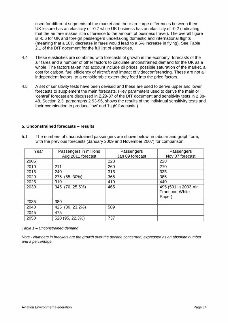
5.1 The numbers of unconstrained passengers are shown below, in tabular and graph form, with the previous forecasts (January 2009 and November 2007) for comparison.

Year Passengers in millions Aug 2011 forecast

Passengers Jan 09 forecast

Passengers Nov 07 forecast

2005 228 228

2010 211 260 270 2015 240 315 335 2020 275 (65, 30%) 365 385 2025 310 410 440 2030 345 (70, 25.5%) 465 495 (501 in 2003 Air

Transport White Paper)

2035 380 2040 425 (80, 23.2%) 589 2045 475 2050 520 (95, 22.3%) 737

Table 1 – Unconstrained demand

Note - Numbers in brackets are the growth over the decade concerned, expressed as an absolute number and a percentage.


5.2 Different components of the model work up to different end dates. The upshot is that

forecasts up to 2030 are the most rigorous and that they become progressively less rigorous afterwards as more assumptions and extrapolations need to be added.

5.3 It can be seen from the table/graph that there has been a huge reduction in forecasts from 2007. The current forecast for 2030 is 31% down as compared with the forecast made in November 2007 (345 mppa rather than 495) and 26% down compared with the forecast made in January 2009 (345 rather than 465). The changes to the growths from 2010 to 2030 that the yearly forecasts represent are even larger at 40% and 33%1. There are a number of reasons why forecasts have changed, but the most signifcant is the recent recession and resulting suspension of aviation growth, affecting the future up to at least 2030. The forecasts in January 2009 started to reflect recession but did not anticipate the full extent of it or its impact on aviation.

5.4 The forecasts shown in Table 1 above are ‘central’ forecasts. These represent DfT’s best estimate, but, recognising that there is a good deal of uncertainty, a number of sensitivity forecasts were carried out. A number of parameters that affect demand were varied in turn and the effect of each on the forecast was calculated2.The largest effects resulted from an assumption that the market would mature faster, lowering the forecast at 2030 by 10%, and by assuming there would be a ‘bounce back’ in demand after recession had finished, increasing the forecast by 12%.

5.5 Table 2.8 of the DfT document shows a set of sensitivity tests, but the results are rounded

to the nearest 5 mppa which somewhat obscures the results. Appendix 2 of this paper shows the unrounded results.

5.6 To reflect the sensitivity tests, a ‘low’ and a ‘high’ set of forecasts were produced. A low

forecast could have been derived on the basis of adding up the decreases due to each sensitivity assumption that caused a reduction and a high forecast correspondingly based

1 The forecast growth from 2010 to 2030 was 495-270=225 in November 2007 and 345-211=134 in August 2011, a

reduction of 40%. For January 2009 the growth from 2010 to 2030 was 460–260=200, a reduction of 33%.

2 Key parameters used to derive the main or ‘central’ forecast are discussed in 2.29-37 of the DfT document and

sensitivity tests in 2.38-48. Section 2.3, paragraphs 2.93-96, discuss the individual sensitivity tests and Table 2.8 shows the results. They are combined to produce ‘low’ and ‘high’ forecasts.


on each sensitivity assumption that caused an increase. However the likelihood of all the sensitivities working in the same direction is low and is made even lower by the fact that some changes of assumption are correlated and will pull in opposite directions. Thus lower GDP growth, tending to lead to a lower forecast, is likely to be associated with a lower oil price (due to less world demand), tending to lead to a higher forecast.

5.7 To derive the more moderate low and high forecasts, DfT have combined the following

sensitivities. The low forecast combines: high market maturity, low GDP, low oil prices, low carbon prices, high exchange rates (i.e. a stronger pound), high fuel efficiency and high video conferencing assumptions. The high forecast combines: low market maturity, high GDP, high oil prices, high carbon prices, low exchange rates (i.e. a weaker pound), low fuel efficiency and low video-conferencing assumptions. It should be noted that some of the sensitivities can pull in different directions. For example, low GDP, one of the sensitivities in the low forecast, pulls the forecast down from the central, while low oil price pushes the forecast back up.

5.8 Table 2.9 of the DfT document shows the sensitivity tests applied incrementally to derive

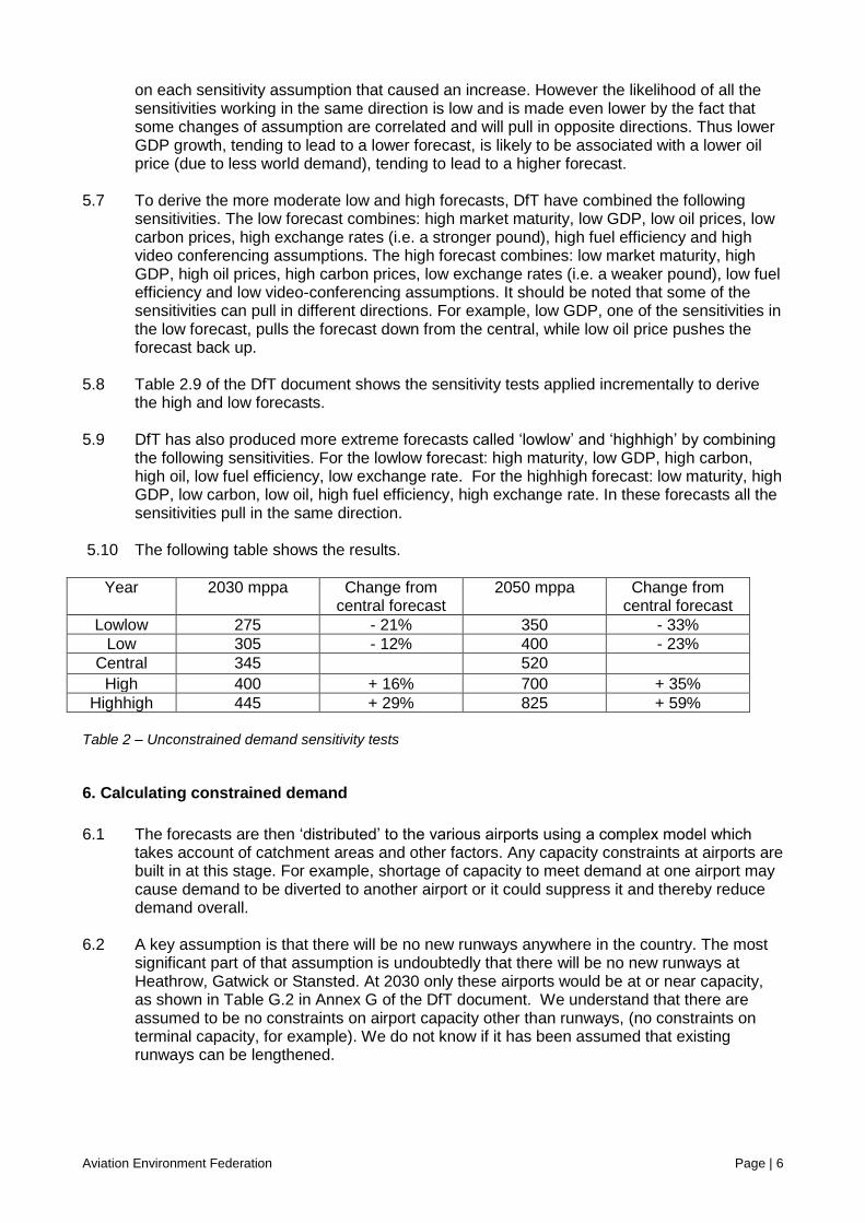
the high and low forecasts. 5.9 DfT has also produced more extreme forecasts called ‘lowlow’ and ‘highhigh’ by combining

the following sensitivities. For the lowlow forecast: high maturity, low GDP, high carbon, high oil, low fuel efficiency, low exchange rate. For the highhigh forecast: low maturity, high GDP, low carbon, low oil, high fuel efficiency, high exchange rate. In these forecasts all the sensitivities pull in the same direction.

5.10 The following table shows the results.

Year 2030 mppa Change from central forecast

2050 mppa Change from central forecast

Lowlow 275 - 21% 350 - 33% Low 305 - 12% 400 - 23%

Central 345 520 High 400 + 16% 700 + 35%

Highhigh 445 + 29% 825 + 59% Table 2 – Unconstrained demand sensitivity tests

6. Calculating constrained demand

6.1 The forecasts are then ‘distributed’ to the various airports using a complex model which

takes account of catchment areas and other factors. Any capacity constraints at airports are built in at this stage. For example, shortage of capacity to meet demand at one airport may cause demand to be diverted to another airport or it could suppress it and thereby reduce demand overall.

6.2 A key assumption is that there will be no new runways anywhere in the country. The most

significant part of that assumption is undoubtedly that there will be no new runways at Heathrow, Gatwick or Stansted. At 2030 only these airports would be at or near capacity, as shown in Table G.2 in Annex G of the DfT document. We understand that there are assumed to be no constraints on airport capacity other than runways, (no constraints on terminal capacity, for example). We do not know if it has been assumed that existing runways can be lengthened.


6.3 As well as forecasting passengers, the report also estimates ATMs (‘air transport movements’ – the number of planes). This is a less fundamental and therefore a less important figure than passengers because most types of impact align more closely with passenger numbers than with flight numbers. Also, estimation of ATMs is subject to more uncertainty than passengers because estimates depend on an extra layer of assumptions concerning aircraft design and fleet mix. We therefore do not consider ATMs further in this report. However, ATMs are very important in the controversial issue of new runways, since runway capacity is largely limited by ATMs, not passengers.

7. Constrained forecasts – results 7.1 The constrained forecasts resulting from the calculations are shown in Table 3 below.

Year Low Central High lowlow highhigh 2010 211 211 211 2015 230 235 250 2020 255 270 (59, 28.0%) 295 2025 275 305 335 2030 300 335 (65, 24.0%) 380 270 420 2035 320 365 430 2040 340 405 (70, 20.1%) 465 2045 365 445 500 2050 380 470 (65, 16.0%) 515 340 525

Table 3 – Constrained forecasts Note - Numbers in brackets are the growth over the decade concerned, expressed as an absolute number and a percentage.

7.2 We also show the ratio between the unconstrained and constrained forecast at each year.

This is important because it shows the effect on passenger numbers of the assumed policy on aviation.

Table 4 – Constrained as percentage of unconstrained demand

7.3 Despite the fact that it is assumed there will be no new runways anywhere in the UK, the constrained forecasts up to 2030 are only slightly less than the unconstrained forecast: just

Year Low Central High lowlow highhigh 2010 100.0 100.0 100.0 2015 100.0 97.9 100.0 2020 98.1 98.2 100.0 2025 96.5 98.4 97.1 2030 98.4 97.1 95.0 98.2 94.4 2035 98.5 96.1 93.5 2040 97.1 95.3 87.7 2045 97.3 93.7 82.0 2050 95.0 90.4 73.6 97.1 63.6


3% for the central forecast as 20303. This shows that the Government decision not to support extra runways at Heathrow, Gatwick and Stansted will have very little effect in dampening demand/supply. Even when an assumption of no runways anywhere else is added, the effect is very slight.

7.4 Capacity constraints thus have very little effect on overall (UK) demand and growth during

this period. For all practical purposes, a ‘predict and provide’ approach for aviation at national level is implied up to 2030. This is the case when demand is viewed at a national level, but is not necessarily the case at a regional or local level. For Heathrow, the ‘predict and provide’ model has been abandoned and the same might become true of Gatwick.

7.5 The pattern is slightly different after 2030. It is assumed by DfT that no new runways are

built right up to 2050 and this means that demand is more constrained by the diminishing spare capacity at existing airports. However, constrained demand is still only 10% less than unconstrained demand by 2050 (under central forecasts).

8. Analysis and comments on the unconstrained forecasts up to 2030

8.1 Our analysis makes the assumption that the mathematical model for unconstrained

forecasts is sound. The model assumptions, namely that demand is largely a function of the growth of the economy and changes in the price of flying, seem sound and have been used by other forecasters. However, there are a number of caveats to this.

8.2 Behavioural changes

8.2.1 There may be socio-political influences on demand that have not been taken into account. The provision of alternatives to flying, or concern among travellers about the environmental impacts of their travel could, for example, act to reduce demand, whereas effective airline advertising or other attempt to boost air travel could make air travel more attractive. The recession’s effect on consumer confidence, exchange rates, and the general state of the tourist market are examples of other influences.

8.2.2 We are not aware of any established methodology which would address these factors, but it seems likely that over the period from 2011 to 2030, fluctuations would even out and thus have much less effect than economic growth or ticket prices.

8.3 Videoconferencing

8.3.1 The potential impact of video-conferencing may have been considerably under-estimated.

8.3.2 A study by WWF-UK, ‘Moving on: why flying less means more for business’ published in 2011, indicated that there was considerable potential for replacement of business flying by video-conferencing and that a large proportion of companies are actively seeking to do this. It does not appear that DfT has taken any account of this evidence, however. (At a meeting in September 2012 between DfT and NGOs, DfT stated that the consultants undertaking work on Marginal Abatement Costs of climate change measures, in parallel to the DfT’s forecasting work, had not been aware of the WWF analysis.) UCL

3 This is somewhat different from previous years. The 2007 unconstrained forecast showed 495 mppa at 2030 instead of 335,

so there would have been a stronger constraint exerted by having no new runways. Unfortunately, a ‘maximum use’ scenario was not published. By 2009 the 2030 unconstrained forecast has been reduced slightly to 465. This time a scenario with no new runways was published – ‘maximum use’. The effect of this constraint reduced demand by 8%.


research indicating that videoconferencing has the potential to cut 30% of business flying similarly may not have been taken into account.

8.3.3 Video-conferencing is subject to a sensitivity test which shows a modest reduction in demand of 7 mppa – 2.0%. However, the effect on business travel will be much greater. Assuming business is 25% of total travel, this implies about 8% substitution. The DfT document (paragraph 2.44) indicates a 10% reduction in business travel but the AEF and DfT figures are within limits of calculation and rounding errors.

8.3.4 In the opposite direction, DfT cites CCC research which “suggests that rather than substituting for business travel, greater telecommunications use accompanies increases in total travel.” This test shows a modest increase in demand of 4 mppa – 1.2%. The effect on business travel will be much greater. Assuming business is 25% of total travel, this implies about 5% substitution. The DfT document assumes an increase of 5%.

8.4 Economic growth

8.4.1 The recession has caused forecasts of economic growth to be revised downwards by the Government and the DfT forecasting model is highly sensitive to GDP.

8.4.2 The change in GDP growth of just 0.25% taken for the sensitivity tests is very small, given the far larger deviations in recent years. In addition to short-term problems deriving from the turmoil in the financial market, issues such as peak oil, climate change and land shortage mean that assumptions of rapidly ever-increasing GDP are no longer safe.

8.4.3 While we can offer no alternative data on which to change the central forecast, the uncertain future could and should be recognised by taking wider limits for GDP growth. -1% instead of -0.25% would not be unreasonable, noting that even this implies significant continuing economic growth of at least 1% pa.

8.4.4. We estimate that a reduction of 1% pa growth of GDP would reduce the forecast by 19% from the central estimate. A reduction of 19% takes the 2030 forecast to 277 mppa. This is well below the ‘low’ forecast of 305 mppa and it is nearly as low as ‘lowlow’ forecast of 275 (rounded to nearest 5m). See Appendix 1 for further comment and details of the calculation.

8.5 Oil prices

8.5.1 For the purpose of the DfT forecasts, oil prices (in real terms) are assumed to increase somewhat between now and 2030 but still be lower in 2030 than they were in 2008. This seems a very optimistic assumption, given forecasts of continuing world economic growth and constant concerns about peak oil.

8.5.2 Following queries raised by AEF about the oil price sensitivity test, DfT has re-run the model. This uses the ‘highhigh’ price assumption and the result is a reduction of demand by 10%. See Appendix 3 for more detail.

8.5.3 The oil price sensitivity test is used to derive an oil price elasticity of - 0.144. We also use the overall price elasticity of demand to derive an oil price elasticity of - 0.15. These figures are entirely consistent, given the approximate nature of the calculation. See Appendix 3.


8.6 Cost of carbon

8.6.1 DfT has assumed that a ‘cost of carbon’ is built into air fares. This is in the form of ‘abatement cost’. (Charging a cost for carbon is in line with the ‘polluter pays principle’ which AEF supports, although in some cases this may be more appropriately paid through a ‘damage cost’.) The cost is estimated by DfT at £70 per tonne of carbon in 2030. The sensitivity tests assume that the cost of carbon is 50% more or 50% less than the central value. This gives rise to a 3% change in passenger forecast either way 2030. See Appendix 4 for calculations. While +-50% may seem a generous margin, given the large uncertainties in costing carbon it is probably reasonable.

8.6.2 The cost of carbon has been assumed which is based on the traded cost estimated by DECC for the year concerned. This means that the airlines are assumed to pay for permits at the traded price and that price is assumed to be equal to the DECC cost for the year concerned. Given the record to date, where carbon prices have been very low, there must be doubts as to whether the very high figures given by DECC will be realised.

8.6.3 As there is a large allocation of free permits under ETS, however, the airlines would not be paying the full cost of their emissions even if the traded cost of permits that they did have to buy was as high as the DECC cost.

8.6.4 Unless measures are taken to ensure the full cost of carbon is paid, demand will tend to be higher than that forecast. In Appendix 4 we calculate the effect on demand if an airline pays only for excess permits and there is no top-up charge to offset the free permits. This increases demand from 343 to 355 mppa, an increase of 3.5%. If the price of permits is far less than the DECC estimate, the demand could rise to 364 mppa, an increase of 6.1%.

8.7 Non-CO2 impact

8.7.1 Carbon represents only about half of the greenhouse gas (GHG) emissions from aviation. Allowing for other GHGs by applying a radiative forcing factor or 1.9 to DECC costs would reduce demand by 5.5%. See Appendix 5 (section 1). Since the carbon cost is a forecast of the EU ETS price, this figure assumes future amendment of the terms under which aviation has been included in the EU ETS.

8.7.1 This estimate does not allow for cirrus cloud formation. If the RF value were to include that, the cost of GHGs and the effect on demand could be much greater.

8.8 Taxes

8.8.1 There is an underlying difficulty with determining a fair rate of taxation for aviation, namely that there is no general policy or philosophy on what should be taxed and at what level. However, we estimate that if VAT and fuel tax were to be applied to aviation at the same rate as is applied to road vehicles (while noting that motorists also pay other taxes such as road tax and VAT on repairs), this would generate around £8bn per annum, even after netting off APD.

8.8.2 DfT assumes that the level of Air Passenger Duty (APD) will remain constant in real terms from 2012 to 2050. In the 2009 forecasts, APD was subtracted from the carbon cost on the grounds that that APD is intended to cover aviation’s climate costs - an argument we reject. This is not mentioned in the 2011 forecasts; we assume therefore that the anomaly has been removed.


8.8.3 While APD is assumed to continue, the forecasts make no mention of the huge tax advantages enjoyed by the aviation industry. We consider that there should be a sensitivity test to show the effect on the forecasts of the introduction of taxes at a level equivalent to those paid by cars. This does not mean that VAT and fuel duty would be the actual taxes levied. Given the legal and practical difficulties of VAT and fuel duty in relation to aviation, the £8bn might be raised in other forms.

8.8.4 We estimate that if fuel were taxed at the same rate as petrol, with duty plus VAT, this would reduce central demand at 2030 by 25%. See Appendix 6. It could be reasonably argued, however, that if fuel were taxed at such rate and APD retained, this would unfairly penalise the aviation industry. If APD is netted off from the fuel tax, the effect is to reduce demand by 19% instead of 25%. It could also be argued that the carbon charge should also be netted off fuel tax. If this is done, the effect is to reduce demand by 16% instead of 25% or 19%.

8.8.5 Which of these estimates is most appropriate is a matter for debate. It depends on what aviation taxes are meant to cover and what equality or otherwise with other sectors is thought appropriate. Although it does not resolve the problem, it is worth noting that in its response to the report of the Environmental Audit Committee (Sixth Report of Session 2010-12), the Government says “The Budget consultation and the subsequent government Response made clear that the government regards the core objective of Air Passenger Duty (APD) to be raising revenues for the Exchequer in a simple, fair and efficient manner.” The response goes on to say that “.. changes in the structure of APD [not in the overall level of APD] have only a negligible effect on CO2.” This indicates that the Government’s view is that any environmental charges should be through other means, such as the EU ETS. However, the response does not imply that APD is necessarily the only possible revenue-raising tax or that the current level of APD should not be raised. VAT, the exemplar of revenue-raising taxes, is far higher than APD.

8.9 External costs

8.9.1 No realistic costs for impacts other than climate, such as noise, air pollution and sterilisation of land around airports are factored into the forecasts. (the ‘polluter pays principle’ has not been fully implemented.) This, together with the low climate costs, means that the price of flying is artificially low as compared with a situation where aviation meets its full social, environmental and economic costs. Demand would be lower if these costs were included.

8.9.2 We do not have estimates of all these external costs. None of the individual costs are likely

to be as large as the cost of climate change. We assume, for illustrative purposes, that together all the other external costs are equal to the climate cost. If a tax or charge were made for the non-climate costs, the effect on demand can be estimated by analogy with the sensitivity test for climate. As shown in Appendix 5, the effect would be to reduce demand by 12%.

8.9.3 Whether these external costs should be netted off from a fuel tax is a matter for debate. It is

difficult to see how this question can be answered without an underpinning taxation policy/philosophy as mentioned in 8.8.1 above.

8.10 Constraints

There is an implicit assumption in the constrained forecasts that there will be no direct constraints placed on air travel because of climate change or for other environmental and social reasons, except insofar as the Government has assumed that there will be no new


runways. However, we showed in Table 4 that the runway constraint is in practice minimal when considered at a UK level up to 2030.

8.11 Range of DfT forecasts

8.11.1 As described in 5.5, a selection of DfT’s sensitivity tests are combined to generate ‘high’ and ‘low’ forecasts in addition to the central ones. The low forecast combines high market maturity, low GDP, low oil prices, low carbon prices, high exchange rates (i.e. a stronger pound), high fuel efficiency and high video conferencing assumptions. See section 2.45 of the DfT document. The upper bound of the forecast range combines low market maturity, high GDP, high oil prices, high carbon prices, low exchange rates (i.e. a weaker pound), low fuel efficiency and low video conferencing assumptions. In addition, the range of forecasts also reflects different assumptions about the extent to which there will be a ‘bounce-back’ of the exceptional loss of demand following the 2008 financial crisis. (It could be argued that bounce-back is a phenomenon that occurs when expenditure is necessary but has been postponed; this might be the case with house maintenance, but will occur to a much lesser extent with air travel which is largely discretionary.)

8.11.2 We agree with the explanation given by DfT of why it is reasonable not to combine all the

sensitivity tests that would drive the forecast down. Likewise for the high forecast. However, we feel it is wrong to combine low GDP with low carbon prices and low oil prices. ‘Low’ GDP is a reduction of only 0.25% per annum and implies growth of 2% or more. Such sustained growth would be entirely compatible with central or even high carbon and oil prices.

8.11.3 It would be incorrect to combine all the sensitivity tests which push the demand down or

combine all the tests that push it up as the probability of all factors operating in one direction is small (probabilities are multiplicative). But even without resorting to probability calculations and statistics, it is clear there must be a good chance of a couple of the major sensitivities working in the same direction. This means that the high and low values should be considerably further away from the central forecast.

8.11.4 The fact that a modest change to just one sensitivity test – economic growth – gives a lower

value than DfT’s low and lowlow forecasts demonstrates that the forecast range on the low side is far too small. We consider the DfT high and low values give a misleading view of the robustness and accuracy of the forecasts. This view is supported by the massive change in the forecasts since 2007. In 2007 the unconstrained forecast was 495 mppa, yet by 2011 it was 345, a reduction of 30%. This reduction is due mainly to the one parameter – the economic growth forecast. Yet the effect is far larger than the respective 12% and 21% reductions that the current low and lowlow forecasts indicate. DfT seems unwilling to recognise in its current forecasts the volatility in the real world that has been amply demonstrated in the last four years.

9 Sensitivity tests 9.1 In the preceding sub-sections, comments have been made on DfT sensitivity tests, or lack

of them, and in some cases an AEF sensitivity test has been made. The AEF tests are summarised below.


Sensitivity test Revised central forecast (mppa)

increase / decrease (from 343 mppa)

Comment

Economic growth 1% p.a. lower

277 - 19% DfT sensitivity test is to reduce growth rate by only 0.25%

Oil price at 2030 67% higher than now

310 -10% This is the same as the DfT figure – see Appendix 3

Add cost of non-CO2 GHGs 326 - 6% Based on RF of 1.9; cirrus not included

Assume airlines continue to get allowance of free ETS permits

355 + 3% ETS allows a large proportion of free permits

Assume cost of ETS permits is negligible instead of DECC forecast

364 + 6% Cost of permits may be much lower than estimated by DECC carbon costs.

Introduction of fuel tax or equivalent

259 - 25% Assumes duty and VAT on fuel at the same rate as petrol

Fuel tax with APD netted off

269 - 22% DfT assumes APD will continue at present in real terms

Fuel tax with APD and carbon tax netted off

288 - 16% Using DECC cost of carbon

Full non-climate costs (illustrative)

304 - 12% Assumes total non-climate cost equal to climate costs

Table 5 – Summary of AEF sensitivity tests

9.2 Given the uncertainties and assumptions in deriving these sensitivity tests, it would a step

too far to combine them to form ‘high’ or ‘low’ forecasts as has been done by DfT with its sensitivity tests. The individual tests nonetheless give a useful perspective on the DfT forecasts.

9.3 The validity of all sensitivity tests and the assumptions which they are testing are all very

much open for debate. However, the sensitivity tests by DfT and AEF (respectively Appendix 2 of the DfT document and table 5 above) allow certain conclusions to be reached in respect of the accuracy and certainly of the DfT forecasts (as at 2030):

There seems to be little justification for ignoring non-CO2 climate costs as a sensitivity test. If they were included, demand would reduce by 6%.

The economic growth sensitivity tests are far too narrow. If growth were 1% per annum less than forecast, demand would reduce by 19%.

Oil prices seem too low (by 2030) and the DfT sensitivity tests show an effect whose small size is not explained.

The effect of tax exemptions is very large – if a full unabated tax on fuel were applied, demand would reduce by 25%.

Unless measures are taken to top up the cost of ETS permits to reflect the full cost of carbon, demand would increase by up to 6%.


10. Comments on the constrained forecasts up to 2030 10.1 As shown in 7.2, the difference between constrained and unconstrained demand up to

2030 is small – just 3% at 2030, suggesting that the Coalition Government’s no new runways policy at the main South East airports was in fact a low-risk approach that will have very little impact during this period. Given that there is very little ‘choking off’ of demand, it would be hard to conclude there would be any serious economic costs in not building new runways at Heathrow, Gatwick and Stansted up to 2030.

10.2 Any constraints on traffic are likely to affect mainly leisure trips because business travel is

far less price elastic Also, business trips are likely to take place anyway, but using different departing and/or interchange airports. Thus any choking off of business travel would be much less than 3%. Since virtually all the arguments currently being advanced about the economic benefits of air travel are in terms of business travel (which represents only about 25% of trips), it is hard to envisage any significant impact on the UK economy as a whole arising from the level of constraint that is being forecast.

10.3 The assumption made in the forecasts is that there will be no new runways anywhere in the

UK, not just at Heathrow, Gatwick and Stansted. That is, the assumption goes well beyond current Government policy.

10.4 It should, however, be noted that the Chancellor George Osborne said in his autumn

budget statement that the Government would “explore all the options for maintaining the UK's aviation hub status with the exception of a third runway at Heathrow”. This implies that new runways in the SE may not, in fact, be ruled out - a potentially major shift in policy.

10.5 The fact that little traffic would be lost up to 2030 is a key difference between the 2003

forecasts and White Paper where there was a large difference between unconstrained and the ‘maximum use’ constrained forecasts.

11. Comments on the unconstrained forecasts after 2030

11.1 The foregoing comments refer to the 2030 forecasts. The forecasts beyond 2030 are

acknowledged in the DfT document to be less reliable. This is partly because certain components of the model do not work beyond 2030 and, more importantly, because forecasting always becomes less reliable the further ahead it goes. This can be seen from fig 1.2 in the DfT document where the ranges widen greatly, and from table 2.8 where the sensitivity impacts increase greatly.

11.2 Table 1 above shows that while growth rates in percentage terms decline in the four

decades up to 2050, there is an increase in the absolute rate of growth. This is largely because it is assumed that there will be continuous economic growth of 2% or more per annum – see table C1 of the DfT document. This is a questionable assumption, however. While it might be argued that issues such as peak oil, climate change and land shortage may not greatly influence economic growth up 2030, we consider this assumption to be unsafe by 2050. For this reason the central forecast may well be too high. We consider that there should be, at the very least, a far more radical sensitivity test which reduces economic growth by far more than 0.25% pa.

12. Comments on the constrained forecasts after 2030


12.1 Beyond 2030, the forecasts of constrained demand become particularly unreliable. As noted above, there would be little constraint up to 2030, even if there are no new runways at all in the UK. But after 2030 constraints build up - by 2050 10% of traffic would be lost. While the Government may be relaxed about 3% of traffic being lost at 2030, it seems very unlikely that it would be sanguine about 10%.

12.2 We consider that the forecasts of constrained demand are misleading, since they are based

on an assumption of no new runways in the UK up to 2050. In fact there is no such Government policy. The policy is only that there will be no runways at the 3 main SE airports and even this is now doubtful following the recent budget statement and Government comments to the effect that options are open in the forthcoming consultation on aviation strategy.

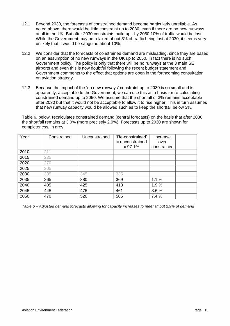
12.3 Because the impact of the ‘no new runways’ constraint up to 2030 is so small and is,

apparently, acceptable to the Government, we can use this as a basis for re-calculating constrained demand up to 2050. We assume that the shortfall of 3% remains acceptable after 2030 but that it would not be acceptable to allow it to rise higher. This in turn assumes that new runway capacity would be allowed such as to keep the shortfall below 3%.

Table 6, below, recalculates constrained demand (central forecasts) on the basis that after 2030 the shortfall remains at 3.0% (more precisely 2.9%). Forecasts up to 2030 are shown for completeness, in grey.

Year Constrained Unconstrained ‘Re-constrained’ = unconstrained

x 97.1%

Increase over

constrained

2010 211 2015 235 2020 270 2025 305 2030 335 345 335 2035 365 380 369 1.1 % 2040 405 425 413 1.9 % 2045 445 475 461 3.6 % 2050 470 520 505 7.4 % Table 6 – Adjusted demand forecasts allowing for capacity increases to meet all but 2.9% of demand


Appendix 1 - Economic growth sensitivity tests 1. The recession has caused forecasts of economic growth to be revised downwards by the

Government. Table C1 of the DfT document shows, after a fall in 2008-15, growth of well over 2% from 2016-30 and 2031-50.

2. The DfT forecasting model is highly sensitive to GDP; an annual reduction of 0.25% in GDP

growth over the period to 2030 produces (from unrounded table 2.8) a 17/343 = 5% reduction in the 2030 forecast for unconstrained demand.

3. The change in GDP growth of just 0.25% taken for the sensitivity tests is very small, given

the far larger deviations seen in recent years. The issue of deviation from past trends is not confined to short-term problems deriving from the turmoil in the financial markets. Issues such as peak oil, climate change and land shortage mean that assumptions of rapid ever-increasing GDP are no longer safe.

4. It is possible that the high rates of growth the UK experienced in the last two decades of up

to 3% per annum were at least partly due to financial activity such as speculation and over-borrowing. That this is not sustainable has been brutally exposed. Despite this, the forecasts do not seem to recognise that in future it may well not be possible to grow at over 2% pa, based on ‘real’ sustainable economic activity.

5. While we can offer no alternative data on which to change the central forecast, the

uncertain future could and should be recognised by taking wider limits for GDP growth. -1% instead of -0.25% would not be unreasonable, noting that even this implies significant continuing economic growth of at least 1% per annum.

6. The data presented in Table 2.8 is heavily rounded, but DfT have provided an ‘unrounded’

version – see Appendix 2. It is actually rounded to 1mppa instead of 5mppa. 7. To minimise the effect of residual roundings, we take the average of the impact of low GDP

and high GDPs. From the unrounded table 2.8, low GDP gives -17 and high GDP gives +18. Total for 0.5% change in GDP is thus 35/343 = 0.102 or 10.2%.

8. Applying this ratio to the central forecast: 343 x (1 - 0.102) = 308.01 for – 0.5% GDP

Apply again 308.01 x (1 – 0.102) = 276.59 ie a drop of 19.4% for – 1.0% GDP. 9. A reduction of 19.4% takes the 2030 forecast to 277 mppa. This is well below the ‘low’

forecast of 305 mppa (rounded) and it is nearly as low as the ‘lowlow’ forecast of 275.


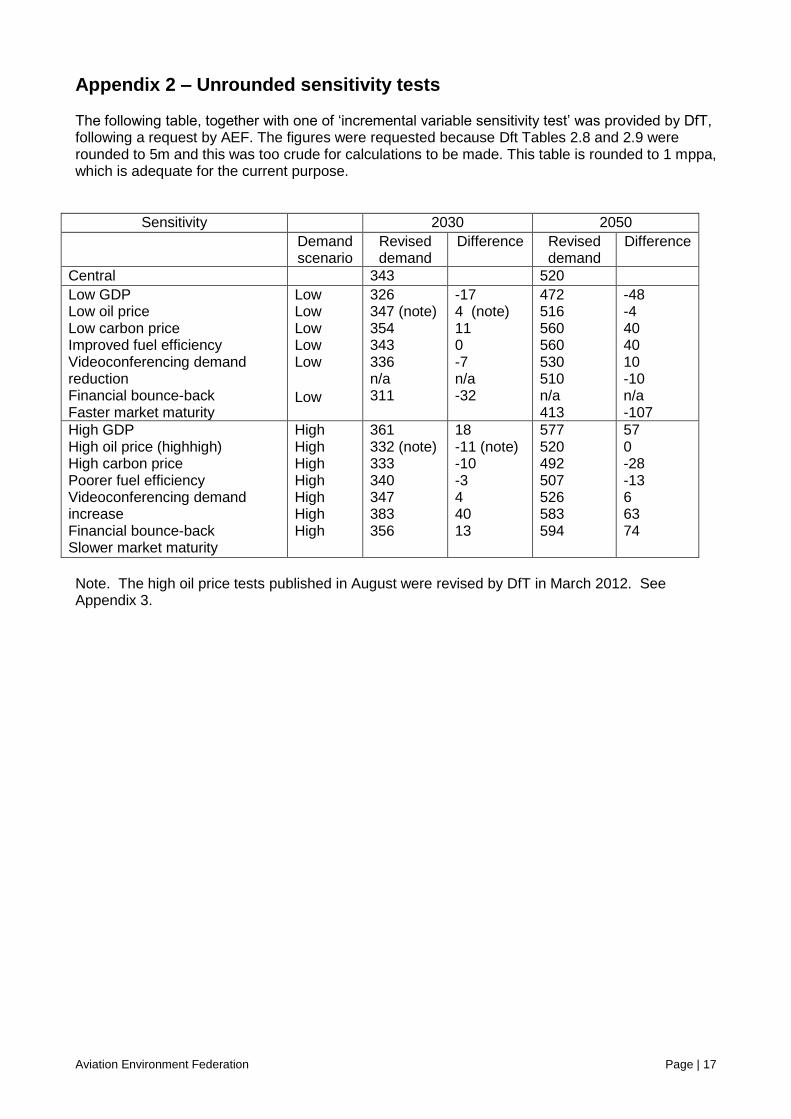
Appendix 2 – Unrounded sensitivity tests

The following table, together with one of ‘incremental variable sensitivity test’ was provided by DfT, following a request by AEF. The figures were requested because Dft Tables 2.8 and 2.9 were rounded to 5m and this was too crude for calculations to be made. This table is rounded to 1 mppa, which is adequate for the current purpose.

Sensitivity 2030 2050

Demand scenario

Revised demand

Difference Revised demand

Difference

Central 343 520 Low GDP Low oil price Low carbon price Improved fuel efficiency Videoconferencing demand reduction Financial bounce-back Faster market maturity

Low Low Low Low Low Low

326 347 (note) 354 343 336 n/a 311

-17 4 (note) 11 0 -7 n/a -32

472 516 560 560 530 510 n/a 413

-48 -4 40 40 10 -10 n/a -107

High GDP High oil price (highhigh) High carbon price Poorer fuel efficiency Videoconferencing demand increase Financial bounce-back Slower market maturity

High High High High High High High

361 332 (note) 333 340 347 383 356

18 -11 (note) -10 -3 4 40 13

577 520 492 507 526 583 594

57 0 -28 -13 6 63 74

Note. The high oil price tests published in August were revised by DfT in March 2012. See Appendix 3.


Appendix 3 - Oil price sensitivity tests 1. DfT sensitivity tests 1.1 For the purpose of the forecasts, oil prices (in real terms) are assumed to increase

somewhat between now and 2030 but still to be lower in 2030 than they were in 2008. Paragraph 2.33 of the DfT document says: “Oil prices are assumed to move in line with the DECC Scenario 2 – "timely investment, moderate demand" oil price projection, which falls from $102 per barrel in 2008 (in 2008 prices) to $70 per barrel in 2010, before rising back to $90 per barrel in 2030.”, taken from ‘Communication on DECC Fossil Fuel Price Assumptions’, DECC, March 2009.

1.2 Table C3 of the DfT document shows a central price of $98 in 2008 falling to $77 in 2010

and rising to $93 at 2030. This seems a very optimistic assumption, given forecasts of world economic growth and continuing concerns about peak oil.

1.3 Section 2.41 of the DfT document says “The oil price test varies the projection of oil prices

within the DECC oil price projection range of $60 per barrel to $150 per barrel (2030 values in 2008 prices).” DfT has advised that the unrounded low, central, high and highhigh prices are respectively $61.68, 92.52, 123.37 and 154.21.

1.4 The DfT publication includes a test for an upper oil price sensitivity, giving a fall in

passenger demand of 343 – 332 = 11mppa or 3.2%. A sensitivity test for a lower oil price gives an increase in passenger demand of 347 – 343 = 4mppa or 1.1%. However, AEF questioned these results and the model was re-run by DfT.

1.5 The results for the highhigh oil price (67% higher than central cost) is demand of 310 mppa.

This is 33 mppa down from the central forecast of 343, a reduction of 9.6%. The result for the low oil price (33% lower than central cost) is 349 mppa. This is 6 mppa up from the central forecast an increase of 1.7%.

2. Oil price elasticity 1.7 It is instructive to compute an elasticity of demand with respect to oil prices. We use the

upper oil price sensitivity test. The increase in oil price in the highhigh test is 67% or 0.667. The resulting decrease in demand is 9.6% or 0.096. The elasticity (dQ/Q)/(dP/P) is therefore 0.096 / 0.667 = 0.144.

1.8 This elasticity is quite low, but this is unsurprising given that oil price is only one of many

factors. There ought to be a relationship to price elasticity because oil prices feed fairly directly into ticket prices - see Section 3 below.

3. Relationship of oil price to overall price elasticity 3.1 As part of its response to the Government’s scoping consultation for its new airports policy,

GACC submitted a paper4 reproducing IATA figures which indicate that fuel was about 25% of European airline costs or 32% as an average of all the world’s major airlines. GACC note that as oil prices have gone down since this analysis was done, fuel costs may now be a lower proportion.

4 ‘Evidence paper 3: The Demand for Air Travel’ http://www.gacc.org.uk/aviation-policy.php

http://www.gacc.org.uk/aviation-policy.php


3.2 It is widely accepted that fuel accounts for around one third of fuel costs on international flights. UK flights do of course include many non-european airlines, though we consider that the figure of 25% (for European airlines) may be a better estimate for UK flights.

3.3 It should also be noted that ticket prices will be equal to costs plus profit. IATA states that

the profit margin for airlines – presumably on turnover – was 2.9% in 20105. This would only reduce a fuel component of 25% to 24.3% (25% / 1.029).

3.4 Allowing for these factors, a figure of 25% (at present) seems reasonable. 3.5 The overall price elasticity estimated by DfT is -0.6 (Table 2.1 of the DfT document). If fuel

costs account for 25% of ticket (ie overall) price, one might expect elasticity to simply be -0.6 x 0.25 = - 0.15.

3.6 This figure is approximate and does not take account of the following factors:

A highly rounded DfT price sensitivity (-0.6)

Application of a single elasticity figure over a rather large price range

The sensitivity test referring to 2030 prices, while the oil percentage of ticket price is the current figure

The fact that refined fuel prices do not change as fast in percentage terms as crude oil prices, because there is a refining cost that is not affected by the market price of crude

The possibility that airlines may not pass on to passengers all the fuel cost increase

3.7 Given these qualifications, especially the rounded value of – 0.6 for overall price elasticity, the oil price elasticity of – 0.144 derived from the oil price sensitivity test compares very well with oil price elasticity of – 0.15 derived from the overall price elasticity,

4. Effect on high and low forecasts 4.1 As noted in 8.11 above, the low forecast assumes lower oil prices and the high forecast

assumes higher oil prices. These assumptions are the reverse of what might be expected – namely that higher oil prices would suppress demand. The reason for this apparently paradoxical result is that higher economic growth is combined with higher oil prices to derive the high forecast and the economic growth has more impact than oil prices. Lower economic growth is likewise combined with lower oil prices in the low forecast.

4.2 The effect of this is that more extreme oil prices, while leading to bigger changes in

forecasts in an individual oil price sensitivity test, pull the high and low forecasts towards the central forecast.

4.3 While we understand the logic of this approach, AEF does not necessarily agree that high

economic growth and high oil prices, which act in opposite directions on passenger forecasts, should be combined in the high forecast. Likewise AEF does not necessarily agree that low economic growth and low oil prices, which also act in opposite directions on passenger forecasts, should be combined in the low forecast.

5 http://gulfnews.com/business/aviation/iata-expects-profitability-of-airlines-to-fall-again-next-year-1.940405

http://gulfnews.com/business/aviation/iata-expects-profitability-of-airlines-to-fall-again-next-year-1.940405


Appendix 4 - Cost of carbon

1. DfT cost of carbon 1.1 DfT has assumed that a ‘cost of carbon’ is built into air fares (in line with the ‘polluter pays

principle’). This is a cost related to achieving emissions targets. 1.2 Box 2.4 says “The current DECC guidance gives a 2010 price of carbon emissions of

£14.1/tCO2e (in 2009 prices), rising to £200/tCO2e (in 2009 prices) by 2050. This guidance is available at: http://www.decc.gov.uk/en/content/cms/emissions/valuation/valuation.aspx”.

1.3 The guidance also provides a range of carbon prices with a lower bound value of

£100/tCO2e and upper bound value of £300/tCO2e (both in 2009 prices) by 2050. This range has been adopted in sensitivity tests.”

1.4 The guidance is called “A brief guide to the carbon valuation methodology for UK policy

appraisal”. The values given for “Real £2011” (October 2011) are as follows.

Year Traded Untraded Low Central High Low Central High

2008 19 19 19 27 53 80 2012 7 14 18 28 56 85 2015 12 19 24 30 59 89 2030 37 74 111 37 74 111 2050 106 212 318 106 212 318 1.5 The DECC document states “In the longer term (2030 onwards) consistent with the

development of a more comprehensive global carbon market, the traded and non-traded prices of carbon will converge into a single traded price of carbon.”

1.6 Prices shown in the DfT forecast document Table 5 are as follows. These are traded

carbon costs and the numbers have been divided by 3.67 to give the numbers in brackets to convert to CO2 costs. This facilitates comparison with the previous table.

Year Low Central High 2008 27 (7) 52 (14) 66 (18) 2015 29 (8) 56 (15) 71 (19) 2030 129 (35) 258 (70) 387 (105) 2050 369 (100) 738 (201) 1107 (302)

1.7 These are 2008 prices. Allowing for price changes between 2008 and 2011, these

numbers are reasonably consistent at 2030, but less so in 2008 or 2015. 2. DfT sensitivity tests 2.1 The prices used in the paper, while not the latest DECC figures, are more relevant in this

context because they are the ones that have been used when deriving sensitivity tests. At 2030, the low and high prices are +50% and -50%. While +-50% may seem a generous margin, it is probably not so, given the large uncertainties in costing carbon.

http://www.decc.gov.uk/en/content/cms/emissions/valuation/valuation.aspx


2.2 From Table 28 of the DfT document (unrounded), the carbon price range gives rise to a (11+10)/343 = 6.1% or c3% each way change in passenger forecast at 2030. The ‘carbon price elasticity’ is (dQ/Q) /(dP/P) = (21/343)/(100/100) = 0.612.

2.3 It is explained in C.23 that the entry of aviation into the ETS is assumed to impact on prices

and therefore the demand forecast. We have been advised by DfT that a cost of carbon has been assumed which is based on the traded cost recommended by DECC for the year concerned.

2.4 This means effectively that the cost of permits is assumed to be equal to the DECC cost.

Given the record to date, however, where carbon prices have been very low, there must be doubts as to whether the very high figures given by DECC will be realised.

2.5 It should also be noted that as there is a large allocation of free permits under ETS, the

airlines would not be paying the full cost of their emissions even if the cost per tonne of permits was equal to the DECC cost.

2.6 Unless measures are taken to ensure the full cost of carbon is paid, demand will tend to be

higher than that forecast. The following estimates the effect on demand if the full cost of carbon is not paid.

3. Sensitivity test for partial payment of carbon costs 3.1 Table H6 in the DfT document estimates that CO2 emissions will rise from 33.4 Mtonnes in

2010 to 47.6 in 2030 (central forecast). The ETS cap will be set at 95% of 2004-6 emissions but airlines will get 85% of these permits free. Emissions have not risen significantly since 2004-6 due to recession, so it can be assumed that airlines will have to pay for 5 + (0.15 x 0.950) = 19.3% of the current requirement of about 33.4 Mt, ie 6.4Mt. At 2030, the airlines will have to pay for the same allowance plus the growth from now until 2030. This is 6.4 + (47.6 – 33.2) = 20.6mt or 43.3% of the requirement.

3.2 If, therefore, ETS is taken to be in lieu of a carbon tax and the price of permits is assumed

to be equal to the DECC price of carbon, the airlines will only have to pay for 19% of their carbon costs now, rising to 43% by 2030.

3.3 The effect on demand can now be calculated using the carbon price elasticity. If only 43.3%

of the carbon is paid for, this is equivalent to paying 43.3% of the full price of all the carbon: a reduction of 56.7% in the cost of carbon. dQ/Q = E x dP/P = 0.612 x 0.567 = 0.0347. dQ = 343 x .0347 = 11.9. The revised demand is thus 343 + 11.9 = 355 or an increase of 3.5%.

3.4 If the permits are cheaper than the DECC price, the demand would be higher than 355. In

the extreme case, where the price is zero, dQ/Q = E x dP/P = 0.612 x 1 = 0.0612. dQ = 343 x .0612 = 21.0. The revised demand is thus 343 + 21 = 364 or an increase of 6.1%. A zero price for permits is equivalent to having no ETS at all for aviation.

3.5 It is not possible to calculate the effect of partial payment of carbon cost in the years up to

2030 because our calculations are based on a DfT sensitivity test, which is only carried out for 2030 (and 2050).

3.6 The impact of carbon dioxide represents only about half of the total greenhouse gas impact

from aviation. See Appendix 5 for calculations.


Appendix 5 – Effect of adding non-CO2 costs to the forecasts

1. Effect of non-CO2 emissions 1.1 The sensitivity test for carbon prices enables the effect of radiative forcing (RF) as a result

of other emissions to be estimated. 1.2 The impact of carbon dioxide represents only about half of the total greenhouse gas impact

from aviation. Although the estimate of non-CO emissions has been dropped in the 2011 forecasts, there is no evidence for a better figure than the factor of 1.9 that was used previously.

1.3 The central carbon price at 2030 is £258. Applying an RF factor of 1.9, the cost for all

GHGs would be 258 x 1.9 = 490, an increase of £232.2. 1.4 In Appendix 4 a ‘carbon price elasticity’ was derived of 0.0612. This can be used to revise

the demand forecast if the price of non-CO2 emissions was paid. (dQ/Q) = E x (dP/P) = 0.0612 x 232.2 / 258 = .0551. dQ = 343 x 0.551 = 18.9. The revised demand is then 343 – 18.9 = 324, a reduction of 5.5%.

1.5 This estimate does not allow for cirrus cloud formation. If the RF factor were to include that,

the cost of GHGs and the effect on demand could be much greater. 1.6 The carbon price used in the DfT paper represents a forecast of the traded price under EU

ETS. Inclusion of non-CO2 costs therefore implies future amendment of the terms of aviation’s inclusion in the EU ETS, or the development of a parallel policy mechanism.

2. Effect of all GHG emissions (CO2 and other impacts combined) 2.1 A carbon cost has already been assumed in generating the central forecast, which is why

the above calculations allow for only the non-CO2 impact. It is, however, useful to derive the impact of CO2 and non-CO2 emissions together. This shows the full effect of charging for climate costs.

2.2 From 1.4 above, inclusion of non-CO2 cost reduces demand by 18.9 mppa from the central

forecast. The effect of the CO2 emissions can be calculated from the elasticity: (dQ/Q) = E x (dP/P) = 0.0612 x 258 /258 = .0612. dQ = 343 x 0.612 = 20.0. The demand would thus be 20 mppa higher than the central forecast if CO2 costs had not been factored in. The impact of CO2 plus non-CO2 charge is therefore 18.9 + 20.0 = 39.9, a total 11.6% reduction.

3. Non-climate costs The result in 2 also enables an additional sensitivity test to be carried out. Section 8.9 of the main report notes that there is no allowance for external costs other than those from climate change. For illustrative purposes it is assumed that the sum of all these non-climate costs is equal to the climate cost. The reduction of 39.9 mppa can be applied to central forecast. The effect is to reduce demand to 343 – 39.9 = 304, a reduction of 11.6%.


Appendix 6 – Effect of fuel tax on the forecasts 1. It has been convincingly argued by AEF and others for some years that fairer tax on flying

would be achieved if aircraft fuel was taxed as the same rate as petrol. We use this as a basis for estimating the effect on demand of different tax regimes.

2. As there is no DfT sensitivity test for alternative tax levels, we represent tax as an increase in oil price and then use the DfT oil price sensitivity test as a baseline for calculating the effect of different tax levels. (The reason for using the oil price sensitivity test is that the effect, as far an airline is concerned, is the same for a tax on fuel as a charge for carbon at the same level.)

3. As noted at http://www.repp.org/repp_pubs/pdf/devGGas.pdf, the carbon content of

kerosene is about 87%. The central cost of carbon at 2030 is £258 per tonne (see Appendix 4). A cost of £258 per tonne of carbon therefore corresponds to 258 x .87 = £224.5 per tonne of kerosene. The Renewable Energy Policy Project also indicates that the weight of kerosene is 0.8kg/litre. The cost is thus 224.6 x 0.80 / 1000 = 18.0p per litre of kerosene.

4. According to http://www.petrolprices.com/the-price-of-fuel.html, each litre of petrol attracts

duty of 57.95p, and VAT of 22.15p. Applying the same rates of tax to aircraft fuel, the tax per litre of kerosene would be 57.95 + 22.15 = 80.1p per litre.

5. As noted in Appendix 1, the mppa changes by 21m for every change in fuel price of £258 and from 1 above, a change in price of carbon of £258 is equivalent to an 18.0p increase per litre of fuel.

6. It is possible to use the carbon price elasticity of 0.612 to produce an adjusted forecast of demand. From 1 above, the ratio dP/P = 1 for an 18.0p per litre tax on fuel. If a tax of 80.1p per litre were applied, dP/P = 1 x 80.1 / 18.0 = 4.45. (dQ/Q) = E x (dP/P) = 0.0612 x 4.45 = .272. dQ = 343 x 0.272 = 93.4.The revised demand would then be 343 – 93 = 250, a reduction of 27%.

7. Price elasticities should ideally be used over a modest range price because there is no assurance that the price elasticity is a single figure which can be applied to a large step change in price. We have no data as to how elasticity will change along the price/demand curve, but in the absence of this we use the same elasticity but apply it stepwise in increments of 18.0p.

8. The stepwise calculations are as follow: No tax 343 mppa 18p per litre 343.0 x (1-0.0612) = 322.0 36 322.0 x (1-0.0612) = 302.3 54 302.3 x (1-0.0612) = 283.8 72 383.8 x (1-0.0612) = 266.4 90 662.4 x (1-0.0612) = 250.1 80.1 by interpolation: 266.4 - (266.4 - 250.1) x (80.1 – 72)/18 = 259.1

9. The demand is thus 259 instead of 250 (see 4 above) so this is a slightly more conservative

approach. We use this stepwise method from here on.

10. The effect of applying duty and VAT to fuel is thus a reduction in demand of 343 – 259 - 84 mppa or 25%.


11. In quoting figures for a tax on fuel, AEF does not argue for a fuel tax strictly along the lines

of equivalence with petrol tax but rather uses this as a ‘proxy’ for fairer approach to taxation of aircraft fuel, potentially allowing for both environmental and purely revenue-raising components. We have therefore netted off APD from the estimated equivalent tax on aircraft fuel.

12. APD currently raises about £2.2bn per annum. From Appendix 7, the full tax on fuel would raise £10.92bn pa. Therefore 2.2/10.92 = 20.1% should be netted off the fuel tax. Instead of tax of 80.1p per litre, the tax would be 69.8p.

13. The effect on demand for a tax of 69.8p per litre can be calculated by interpolation from 6 above: 283.8 - (283.8 – 266.4) x (69.8 – 54)/18 = 268.5 mppa. The effect of applying duty and VAT to fuel but netting off APD is thus a reduction 75 mppa or 22%.

14. Using similar reasoning, it could be argued that the assumed carbon tax should also be netted off. As noted above, this is equivalent to 18.0p per litre. Subtracting this also, the tax would 69.8 – 18.0 = 51.8p. The effect on demand of a tax of 51.8p per litre can be calculated by interpolation from point 8 above: 302.3 - (302.1 – 283.8) x (51.8 – 36)/18 = 288.0. The effect of applying duty and VAT to fuel but netting off APD and carbon tax would thus be to reduce demand by 55 mppa; a reduction in demand of 16.0%.


Appendix 7 – Tax rates and conversions

1. Fuel taxes and conversions 1.1 From DECC 2009 inventory Table 8: Greenhouse gas emissions arising from use of fuels

from UK international aviation and shipping bunkers and Table 4: Estimated emissions of carbon dioxide (CO2) by National Communication source category, type of fuel and end-user category, 1970-2009:

Int av Dom av Total

07 35.4 2.6 37.0 08 34.2 2.3 36.5 09 32.7 2.1 34.8

1.2 34.8 CO2 is 34.8x12/44 = 9.49 mtC. Weight of kerosene is 0.8kg/l and C content is 87% so

C is .696kgC/l. Therefore fuel used is 1m x 9.49m /0.696 = 13.63bn litres. 1.3 At 80.1p duty+VAT - 13.63 x 0.801 = £10.9bn 1.4 To split out duty and VAT:

Duty 57.95 x 13.63 = £7.90bn VAT 22.15 x 13.63 = £3.02bn Total £10.92bn

1.5 If VAT only were charged on the non-duty component of petrol:

Product + retail = 47.8 + 5 (from ://www.petrolprices.com/the-price-of-fuel.html) = 52.5 x 20% = 10.56p 10.56p x 13.63bn = £1.44bn.

2. Statements about APD 2.1 2.35 of 2011 Budget, HM Treasury, March 2011, HC 836: “APD rates are assumed to

remain constant in real terms beyond the rates announced in the 2011 Budget”. 14.2 2.140 of budget statement – “Aviation tax: rates (Finance Bill 2012) (36): Air Passenger

Duty (APD) rates will be frozen for 2011-12. The RPI increase assumed in the forecast will be deferred and implemented alongside the April 2012 RPI increase.”

uk air passenger demand forecasts briefing · aviation environment federation page | 1 uk air...

Documents