Çukurova university institute of natural and …
TRANSCRIPT

ÇUKUROVA UNIVERSITY INSTITUTE OF NATURAL AND APPLIED SCIENCES
MSc THESIS
Murat Mustafa SAVRUN
DESIGN AND SIMULATION OF THYRISTOR SWITCHING SYSTEM FOR REACTIVE POWER CONTROL AND MOTOR POWER EFFICIENCY CONTROL
DEPARTMENT OF ELECTRICAL AND ELECTRONICS ENGINEERING
ADANA, 2013

ÇUKUROVA UNIVERSITY INSTITUTE OF NATURAL AND APPLIED SCIENCES
DESIGN AND SIMULATION OF THYRISTOR SWITCHING SYSTEM FOR
REACTIVE POWER CONTROL AND MOTOR POWER EFFICIENCY CONTROL
Murat Mustafa SAVRUN
MSc THESIS
DEPARTMENT OF ELECTRICAL AND ELECTRONICS ENGINEERING We certify that the thesis titled above was reviewed and approved for the award of degree of the Master of Science by the board of jury on 06/08/2013.
................................................ ........................................................ ............................................................. Prof. Dr. Mehmet TÜMAY SUPERVISOR
Asst. Prof. Dr. M. Ugraş CUMA MEMBER
Assoc. Prof. Dr. Ramazan ÇOBAN MEMBER
This MSc Thesis is written at the Department of Institute of Natural And Applied Sciences of Çukurova University. Registration Number:
Prof. Dr. Mustafa GÖK Director Institute of Natural and Applied Sciences
Note: The usage of the presented specific declerations, tables, figures, and photographs either in this
thesis or in any other reference without citiation is subject to "The law of Arts and Intellectual Products" number of 5846 of Turkish Republic.
I
ABSTRACT
MSc THESIS
DESIGN AND SIMULATION OF THYRISTOR SWITCHING SYSTEM FOR REACTIVE POWER CONTROL AND MOTOR POWER
EFFICIENCY CONTROL
Murat Mustafa SAVRUN
ÇUKUROVA UNIVERSITY INSTITUTE OF NATURAL AND APPLIED SCIENCES
DEPARTMENT OF ELECTRICAL ELECTRONICS ENGINEERING Supervisor : Prof. Dr. Mehmet TÜMAY Year: 2013, Pages: 129 Jury : Prof. Dr. Mehmet TÜMAY : Asst. Prof. Dr. M. Uğraş CUMA : Assoc. Prof. Dr. Ramazan ÇOBAN
Nowadays, the majority of the increasing energy consumption is consumed by industrial organizations that are constantly growing and evolving. A large part of the energy used in industry is consumed by electric motors. As a result of work to be done on the efficiency of electric motors, large declines in energy consumption values can be established.
In this study, a new motor drive which is designed to provide efficiency in asynchronous motor that is the most commonly used industry is presented. The driver is modeled in PSCAD/EMTDC. Designed driver provides energy-efficiency in motors which operating at lightly loads. The proposed methods provide superior performance compared to conventional methods.
The aim of the thesis is that design and simulation a motor drive which provide energy efficiency in 7.5 kW induction motor. The performance and provided efficiency values of the proposed motor driver are investigated with different simulation studies by PSCAD program.
Key Words: Asynchronous Motor Control, Flux Control, Energy Efficiency, Stator
Voltage Control

II
ÖZ
YÜKSEK LİSANS TEZİ
REAKTİF GÜÇ KONTROLÜ VE MOTOR ENERJİ VERİMLİLİĞİ KONTROLÜ İÇİN TRİSTÖR ANAHTARLAMA SİSTEMİ TASARIMI VE
SİMÜLASYONU
Murat Mustafa SAVRUN
ÇUKUROVA ÜNİVERSİTESİ FEN BİLİMLERİ ENSTİTÜSÜ
ELEKTRİK ELEKTRONİK MÜHENDİSLİĞİ ANABİLİM DALI
Supervisor : Prof. Dr. Mehmet TÜMAY Year: 2013, Pages: 129 Jury : Prof. Dr. Mehmet TÜMAY : Yrd. Doç. Dr. M. Uğraş CUMA : Doç. Dr. Ramazan ÇOBAN
Günümüzde artan enerji tüketiminin büyük çoğunluğuna sürekli olarak büyüyen ve gelişen endüstriyel kuruluşlar sahiptir. Endüstride kullanılan enerjinin büyük bir kısmı ise elektrik motorları tarafından tüketilmektedir. Bu nedenle de elektrik motorları üzerine yapılacak bir verimlilik çalışması sonucunda enerji tüketim değerlerinde büyük düşüşler sağlanabilecektir.
Bu çalışmada endüstride en çok kullanılan motor tipi olan asenkron motorda verimlilik sağlayabilmek için tasarlanmış olan yeni bir motor sürücü sunulmuştur. Sürücü PSCAD/EMTDC programı kullanılarak modellenmiştir. Tasarlanan sürücü düşük yüklerde çalışan motorlarda enerji verimliliği sağlamaktadır. Önerilen metot var olan metotlara göre üstün bir performans sağlamaktadır.
Tezin amacı 7,5 kW’lık bir asenkron motorda enerji verimliliği sağlayacak bir motor sürücüsü tasarlamak ve simülasyonunu yapmaktır. Önerilen motor sürücüsünün performansı ve sağladığı verimlilik değerleri PSCAD programında farklı simülasyon çalışmalarıyla incelenmiştir.
Anahtar Kelimeler: Asenkron Motor Kontrol, Akı Kontrol, Enerji Verimliliği,
Stator Gerilim Kontrol

III
ACKNOWLEDGEMENTS
The subject of this thesis was suggested by my supervisor, Prof. Dr. Mehmet
Tümay to whom I would like to express my heartfelt thanks for his supervision,
guidance, encouragements and extremely useful suggestions throughout this thesis. It
has been a great honor to have Prof. Dr. Mehmet Tümay as supervisor.
I would like to thank Assoc. Prof. Dr. K. Çağatay Bayındır for his extremely
valuable guidance and suggestions throughout in the thesis. His technical assistance
and personal advice have been invaluable.
I would also like to thank you to Asst. Prof. Dr. M. Uğraş Cuma for his
valuable advices and strong technical support. Their continuous support helped me to
finish this thesis.
I wish to thank Institute of Natural and Applied Science for financial supports
during the preparation of this thesis. I wish also to extend my acknowledgements to
all staff members in the department and my friends.
Finally, I would like to thank my family for their endless support and
encouragements.
Murat Mustafa SAVRUN

IV
CONTENTS PAGE
ABSTRACT ............................................................................................................. I
ÖZ ........................................................................................................................................... II
ACKNOWLEDGEMENTS ............................................................................................... III
CONTENTS ......................................................................................................................... IV
LIST OF TABLES ............................................................................................................... VI
LIST OF FIGURES .......................................................................................................... VIII
LIST OF SYMBOLS........................................................................................................ XIV
LIST OF ABBREVATIONS .......................................................................................... XVI
1. INTRODUCTION ............................................................................................................. 1
1.1. Outline of Dissertation............................................................................................... 2
2. LITERATURE REVIEW ................................................................................................. 3
2.1. Introduction ................................................................................................... 3
2.2. Conclusion of Literature Review ................................................................. 25
3. ENERGY EFFICIENCY METHODS ON MOTORS ............................................... 27
3.1. Motor Starting Methods .......................................................................................... 28
3.1.1. Direct-On-Line Starting Method ......................................................... 29
3.1.2. Shunt Capacitance Method ................................................................. 30
3.1.3. Delta-Wye Starting Method ................................................................ 30
3.1.4. Autotransformer Method .................................................................... 31
3.1.5. Series Resistance or Reactance Method .............................................. 32
3.1.6. Soft Starter Method ............................................................................ 33
3.1.7. Variable Frequency Drive ................................................................... 34
3.2. High Efficiency Induction Motors ............................................................... 37
4. MOTOR DRIVER MODELING .................................................................................. 39
4.1. Mathematical Modeling............................................................................... 40
4.2. Power Circuit Model ................................................................................... 44
4.2.1. Motor Parameters .............................................................................. 45
4.2.2.Thyristor Block Design ...................................................................... 50
4.3. Proposed Fuzzy Logic Based Control System .............................................. 51

V
4.3.1. Torque Estimator Block Design ......................................................... 52
4.3.2. Firing Angle Generation Block Design .............................................. 53
4.3.3. FL Based Firing Angle Optimization Block Design ........................... 55
4.3.3.1. Fuzzy Logic System ................................................................ 55
4.3.3.1.(1). Rules ...................................................................... 56
4.3.3.1.(2). Fuzzy Inference Engine .......................................... 57
4.3.3.1.(3). Fuzzification ........................................................... 58
4.3.3.1.(4). Defuzzification ....................................................... 58
4.3.3.2. Fuzzy Logic Controller Modeling ........................................... 60
4.3.3.2.(1). Fuzzification ........................................................... 61
4.3.3.2.(2). Decision Making ..................................................... 66
4.3.3.2.(3). Defuzzification ....................................................... 70
4.4. Over and Under Voltage Protection Unit ..................................................... 73
4.5. Over Current Protection Unit ....................................................................... 74
5. SIMULATION RESULTS ............................................................................................. 75
5.1. Proposed PSCAD Model and System Parameters ........................................ 75
5.2. Case 1: No Load .......................................................................................... 77
5.3. Case 2: 10% Loaded .................................................................................... 83
5.4. Case 3: 20% Loaded .................................................................................... 88
5.5. Case 4: 30% Loaded .................................................................................... 94
5.6. Case 5: 40% Loaded .................................................................................. 100
5.7. Case 6: 50% Loaded .................................................................................. 106
5.8. Case 7: Dynamic Performance .................................................................. 112
5.9. Case 8: Short Circuit Performance ............................................................. 114
6. CONCLUSION .............................................................................................................. 117
REFERENCES ................................................................................................................... 123
BIOGRAPHY ..................................................................................................................... 129

VI
LIST OF TABLES PAGE
Table 2.1. Measure Data (Hui et al., 2005) ............................................................ 13
Table 4.1. Codes of Torque Estimator Block ......................................................... 52
Table 4.2. Codes of Firing Angle Generation Block .............................................. 54
Table 4.3. Linguistic terms for the error, erate and Δα ........................................... 62
Table 4.4. Input Ranges of error and error_rate ..................................................... 64
Table 4.5. Membership Function Codes of error ................................................... 64
Table 4.6. Membership Function Codes of error_rate ............................................ 65
Table 4.7. Rule Base for the FL Controller ............................................................ 66
Table 4.8. FL Controller Decision Rules ............................................................... 68
Table 4.9. FL Rule Base Fuzzy Logic Controller .................................................. 69
Table 4.10. Fuzzy Decision Rule Table of Example ................................................ 70
Table 5.1. System Parameters ............................................................................... 75
Table 6.1. FL Power and Power Factor Efficiency .............................................. 121

VII

VIII
LIST OF FIGURES PAGE
Figure 2.1. Iron Losses, Stator and Rotor Copper Losses and Total Losses for 20
HP motor running at 20 % load factor under variable voltages (Pitis
et al., 2008) ......................................................................................... 4
Figure 2.2. Power consumption of capacitor-start, capacitor-run, 2-hp single-
phase induction motor with and without controller (Fuchs et al.,
2002).................................................................................................... 5
Figure 2.3. Power factor (PFcontr) of controller and displacement factor
(DFmot) of capacitor-start, capacitor-run, 2-hp single-phase
induction motor with (PFcontr) and without (DFmot) controller
(Fuchs et al., 2002) ............................................................................... 6
Figure 2.4. Power consumption of 7.5-hp three-phase Y -connected three-phase
motor with and without controller (Fuchs et al., 2002) .......................... 6
Figure 2.5. Power factor of 7.5-hp three-phase Y -connected three-phase motor
with and without controller (Fuchs et al., 2002) .................................... 6
Figure 2.6. AC Voltage Controller Under Induction Motor Load (Eltamaly et al.,
2007).................................................................................................... 8
Figure 2.7. Controlling of Three-Phase Induction Motor Using MPAC and EAC
Strategies (Eltamaly et al., 2007) .......................................................... 8
Figure 2.8. Triac in Series for Induction Motor Voltage Control (Benbouzid et
al., 1996) ............................................................................................ 10
Figure 2.9. Voltage and Current Waveforms of Power Circuit (Benbouzid et al.,
1996).................................................................................................. 11
Figure 2.10. Thyristor Power Test Circuits (Paice, 1968) ....................................... 14
Figure 2.11. Matlab/Simulink Simulation Model Used to Generate Data for ANN
Training (Gastli et al., 2005) .............................................................. 17
Figure 2.12. Torque Versus Speed Characteristics for Different Values of The
Thyristors Firing Angle (Gastli et al., 2005) ....................................... 17
Figure 2.13. Structure of ANFIS AC Voltage Controller (Ayyub, 2006) ................ 19
Figure 2.14. Simulation Model with ANFIS Controller (Ayyub, 2006) .................. 20

IX
Figure 2.15. Proposed ANFIS Based Soft Starter Strategy (Rajaji et al., 2008) ....... 22
Figure 2.16. The Schematic Block Diagram of Soft Starting System with Fuzzy
Adaptive Control (Dayong et al., 2011) .............................................. 23
Figure 3.1. Direct-On-Line Starter Circuit Diagram ............................................. 29
Figure 3.2. Soft Starter Circuit Diagram ............................................................... 34
Figure 3.3. VFD Circuit Diagram (Mistry et al., 2012) ......................................... 35
Figure 4.1. Equivalent Circuit of an Induction Motor ........................................... 41
Figure 4.2. Power Flow Diagram of an Induction Motor ...................................... 41
Figure 4.3. Typical Waveforms of Single-Phase Stator Voltage Controller with
an R-L Load. ...................................................................................... 44
Figure 4.4. Power Diagram of Proposed Motor Drive .......................................... 45
Figure 4.5. Squirrel Cage Induction Motor Model ................................................ 45
Figure 4.6. Squirrel Cage Induction Motor Parameter Setting .............................. 46
Figure 4.7. Modeled Motor a) Active Power, b) Reactive Power .......................... 47
Figure 4.8. Modeled Motor Phase a) Voltage Waveform b) Current Waveform.... 48
Figure 4.9. Modeled Motor a) No-Load Speed b) Full-Load Speed ...................... 49
Figure 4.10. Symmetrical AC Voltage Controller of Driver ................................... 50
Figure 4.11. Firing Sequence of Thyristors ............................................................ 51
Figure 4.12. The Whole of Proposed Fuzzy Logic Based Control System .............. 51
Figure 4.13. Firing Angle Generation Block .......................................................... 52
Figure 4.14. Firing Angle Generation Block .......................................................... 53
Figure 4.15. Torque versus Firing Angle Characteristics. ....................................... 54
Figure 4.16. Fuzzy Logic System ........................................................................... 56
Figure 4.17. Max-min Inference (Cuma, 2006) ...................................................... 58
Figure 4.18. Proposed FL Control System Block Diagram ..................................... 61
Figure 4.19. Proposed FL Control System Block Diagram of PSCAD ................... 61
Figure 4.20. Membership Function of Input 1 - error ............................................. 62
Figure 4.21. Membership Function of Input 2 - error_rate ...................................... 62
Figure 4.22. Input of error Signal ........................................................................... 69
Figure 4.23. Input of error_rate Signal ................................................................... 70
Figure 4.24. Firing Pulse Generation Block ........................................................... 72

X
Figure 4.25. Firing Pulses for Each Thyristors ....................................................... 72
Figure 4.26. Over Voltage Protection Unit ............................................................. 73
Figure 4.27. Under Voltage Protection Unit ........................................................... 74
Figure 4.28. Over Current Protection Unit ............................................................. 74
Figure 5.1. Circuit Diagram of Motor Driver ........................................................ 76
Figure 5.2. Motor Load Voltage With_Driver ...................................................... 77
Figure 5.3. Motor Load Voltage Without_Driver ................................................. 77
Figure 5.4. Motor Load Current With_Driver ....................................................... 78
Figure 5.5. Motor Load Current With_Driver in Large Scale ............................... 78
Figure 5.6. Motor Load Current Without_Driver .................................................. 79
Figure 5.7. Motor Input Power With_Driver ........................................................ 79
Figure 5.8. Motor Input Power Without_Driver ................................................... 80
Figure 5.9. Motor Input Reactive Power With_Driver .......................................... 80
Figure 5.10. Motor Input Reactive Power Without_Driver ..................................... 81
Figure 5.11. Speed of Motor With_Driver .............................................................. 82
Figure 5.12. Speed of Motor Without_Driver ......................................................... 82
Figure 5.13. Motor Load Voltage With_Driver ...................................................... 83
Figure 5.14. Motor Load Voltage Without_Driver ................................................. 83
Figure 5.15. Motor Load Current With_Driver ....................................................... 84
Figure 5.16. Motor Load Current With_Driver in Large Scale ............................... 84
Figure 5.17. Motor Load Current Without_Driver .................................................. 85
Figure 5.18. Motor Input Power With_Driver ........................................................ 85
Figure 5.19. Motor Input Power Without_Driver ................................................... 86
Figure 5.20. Motor Input Reactive Power With_Driver .......................................... 86
Figure 5.21. Motor Input Reactive Power Without_Driver ..................................... 87
Figure 5.22. Speed of Motor With_Driver .............................................................. 87
Figure 5.23. Speed of Motor Without_Driver ......................................................... 88
Figure 5.24. Motor Load Voltage With_Driver ...................................................... 89
Figure 5.25. Motor Load Voltage Without_Driver ................................................. 89
Figure 5.26. Motor Load Current With_Driver ....................................................... 90
Figure 5.27. Motor Load Current With_Driver in Large Scale ............................... 90

XI
Figure 5.28. Motor Load Current Without_Driver .................................................. 91
Figure 5.29. Motor Input Power With_Driver ........................................................ 91
Figure 5.30. Motor Input Power Without_Driver ................................................... 92
Figure 5.31. Motor Input Reactive Power With_Driver .......................................... 92
Figure 5.32. Motor Input Reactive Power Without_Driver ..................................... 93
Figure 5.33. Speed of Motor With_Driver .............................................................. 93
Figure 5.34. Speed of Motor Without_Driver ......................................................... 94
Figure 5.35. Motor Load Voltage With_Driver ...................................................... 95
Figure 5.36. Motor Load Voltage Without_Driver ................................................. 95
Figure 5.37. Motor Load Current With_Driver ....................................................... 96
Figure 5.38. Motor Load Current With_Driver in Large Scale ............................... 96
Figure 5.39. Motor Load Current Without_Driver .................................................. 97
Figure 5.40. Motor Input Power With_Driver ........................................................ 97
Figure 5.41. Motor Input Power Without_Driver ................................................... 98
Figure 5.42. Motor Input Reactive Power With_Driver .......................................... 98
Figure 5.43. Motor Input Reactive Power Without_Driver ..................................... 99
Figure 5.44. Speed of Motor With_Driver .............................................................. 99
Figure 5.45. Speed of Motor Without_Driver ....................................................... 100
Figure 5.46. Motor Load Voltage With_Driver .................................................... 101
Figure 5.47. Motor Load Voltage Without_Driver ............................................... 101
Figure 5.48. Motor Load Current With_Driver ..................................................... 102
Figure 5.49. Motor Load Current With_Driver in Large Scale ............................. 102
Figure 5.50. Motor Load Current Without_Driver ................................................ 103
Figure 5.51. Motor Input Power With_Driver ...................................................... 103
Figure 5.52. Motor Input Power Without_Driver ................................................. 104
Figure 5.53. Motor Input Reactive Power With_Driver ........................................ 104
Figure 5.54. Motor Input Reactive Power Without_Driver ................................... 105
Figure 5.55. Speed of Motor With_Driver ............................................................ 105
Figure 5.56. Speed of Motor Without_Driver ....................................................... 106
Figure 5.57. Motor Load Voltage With_Driver .................................................... 107
Figure 5.58. Motor Load Voltage Without_Driver ............................................... 107

XII
Figure 5.59. Motor Load Current With_Driver ..................................................... 108
Figure 5.60. Motor Load Current With_Driver in Large Scale ............................. 108
Figure 5.61. Motor Load Current Without_Driver ................................................ 109
Figure 5.62. Motor Input Power With_Driver ...................................................... 109
Figure 5.63. Motor Input Power Without_Driver ................................................. 110
Figure 5.64. Motor Input Reactive Power With_Driver ........................................ 110
Figure 5.65. Motor Input Reactive Power Without_Driver ................................... 111
Figure 5.66. Speed of Motor With_Driver ............................................................ 111
Figure 5.67. Speed of Motor Without_Driver ....................................................... 112
Figure 5.68. Dynamic Performance With_Driver ................................................. 113
Figure 5.69. Dynamic Performance Without_Driver ............................................ 113
Figure 5.70. Comparison of Power Consumption in Dynamic Performance ......... 114
Figure 5.71. Comparison of Power Consumption in Dynamic Performance ......... 115
Figure 5.72. Comparison of Power Consumption in Dynamic Performance ......... 115
Figure 5.73. Comparison of Power Consumption in Dynamic Performance ......... 116
Figure 6.1. Comparison of Load Voltage with and without Driver ..................... 118
Figure 6.2. Comparison of Load Current with and without Driver ...................... 119
Figure 6.3. Comparison of Load Current with and without Driver ...................... 119
Figure 6.4. Comparison of Motor Speeds with and without Driver ..................... 120
Figure 6.5. Comparison of Power Consumptions with and without Driver.......... 120
Figure 6.6. Comparison of Power Factors with and without Driver .................... 121

XIII

XIV
LIST OF SYMBOLS
α : Firing Angle
φ : Phase Angle
θ : Conduction Angle
γ : Holdoff Angle
BRK : Breaker
Eload : Load Voltage
f : Fundamental Supply Frequency
IA : Phase A Current
IA_RM : Phase A RMS Current
IB : Phase B Current
IB_RMS : Phase B RMS Current
IC : Phase C Current
IC_RMS : Phase C RMS Current
Iload : Load Current
Iref : References Current
Pcore : Stator Core Loss
PF&W : Friction and Windage Losses
Pin : Input Power
Pmisc : Stray Losses
Pout : Output Power
Pr_core : Rotor Core Loss
PRCL : Rotor Copper Loss
PSCL : Stator Copper Loss
Qin : Input Reactive Power
R1 : Stator Resistance
R2 : Rotor Resistance
S : Select
Speed : Motor Speed
T : Torque

XV
t : Time
Te : Electrical Torque
TL : Load Torque
Tm : Mechanical Torque
tn : Time Instant
Tref : Reference Torque
Trq : Electrical Torque of Motor
TrqRMS : RMS Value of Torque
U : Voltage
VA : Phase A Voltage
VA_RMS : Phase A RMS Voltage
VB : Phase B Voltage
VB_RMS : Phase B RMS Voltage
VC : Phase C Voltage
VC_RMS : Phase C RMS Voltage
Vref : References Voltage
w : Angular Frequency
wm : Motor Speed
wref : Reference Speed

XVI
LIST OF ABBREVATIONS
AC : Alternative Current
ANFIS : Adaptive Neuro Inference System
ANN : Artifical Neural Network
ASD : Adjustable Speed Drive
BN : Big Negative
BP : Big Positive
COG : Centre of Gravity
DC : Direct Current
DOL : Direct On-Line
DS : Decision
EAC : Extinction Angle Control
FL : Fuzzy Logic
FLBEC : Fuzzy Logic Based Efficiency Controller
FLC : Fuzzy Logic Control
FP : Firing Pulse
HM : Height Method
HP : Horse Power
IGBT : Insulated Gate Bipolar Transistor
IM : Induction Machine
LD : Large Decrease
LI : Large Increase
MD : Medium Decrease
Mem.V. : Membership Value
MFs : Membership Function
MI : Medium Increase
MN : Medium Negative
MOM : Mean of Maximum
MP : Medium Positive
MPAC : Modified Phase Angle Control

XVII
N : Neutral
PAC : Phase Angle Control
PF : Power Factor
PSCAD/EMTDC : Power System Computer Aided Design /
Electromagnetic Transient DC Program
PSIM : Power Simulation
PWM : Pulse Width Modulation
SCR : Silicon Controlled Rectifier
SD : Small Decrease
SI : Small Increase
SN : Small Negative
SP : Small Positive
TEFC : Totally Enclosed, Fan Cooled
THD : Total Harmonic Distortion
VFD : Variable Frequency Drive
VVCF : Variable Voltage-Constant Frequency
Z : Zero

1. INTRODUCTION Murat Mustafa SAVRUN
1
1. INTRODUCTION
In globalizing world, the energy consumption is increasing at an exponential
rate due to the exponential growth of world population, industrial developments and
the world economy. In parallel with this rapidly increase in energy consumption, the
fossil energy sources will be exhausted in the near future that has been revealed by
scientific studies. Considering these situations, the world has to seek alternative
solutions. In Turkey, as in many countries of the world, the importance given to the
use of renewable energy sources and energy efficiency studies is increasing day by
day. Within this operation, new policies and regulations are determined. Incentive
mechanisms are created for the use of renewable energy sources and the legal
changes are being made for the energy efficiency studies. The world aims to use the
clean energy as more efficient.
The industrial sector is the largest users of energy around the world.
Industrial motor uses a major fraction of total industrial energy uses (Saidur, 2010).
The induction motor is very popular in industrial production due to its simple
structure, reliability, low cost, convenient maintenance and long life (Li, Liu 2009).
So, these devices are widely used as an electric drives in various industrial
applications, such as pumps, fans, compressors, conveyors, spindles, to name just a
few, as well as in main powered home appliances (Patil et al., 2009).
Due to the vast majority of the energy is consumed by the electric machines
in industrial organizations; as a result of work to be done on the efficiency of electric
motors, large reductions in energy consumption values can be established. In this
context, many efficiency studies were carried out for many years. These efficiency
methods are variety starting methods, motor drive methods, use of high efficient
motors etc.
As a result, the purpose of this study is to design a motor driver that provide
energy efficiency in induction motors and is to simulate in PSCAD software.

1. INTRODUCTION Murat Mustafa SAVRUN
2
1.1. Outline of Dissertation
In Chapter 2, previous studies are mentioned about thyristor controlled motor
drivers which are studied by different researchers. Also, suitable models are prepared
for comparison with available studies in the literature.
In Chapter 3, energy efficiency methods which are used nowadays are
explained.
In Chapter 4, the power circuit configuration and control methods of driver
are described in detail. Fuzzy logic based firing angle determination and protection
units are also elaborated.
In Chapter 5, simulation results for different case studies are given and
evaluated. In these cases, the performance of driver for different loads is analyzed;
dynamic response of driver during variable load change is also investigated.
In Chapter 6, the important conclusions of the study and author’s
recommendations for future work are explained.
Finally, related references used in the thesis and biographical information of
the author are presented.

2. LITERATURE REVIEW Murat Mustafa SAVRUN
3
2. LITERATURE REVIEW
2.1. Introduction
Different studies have been made and are available in the literature about
motor power efficiency control. Also, the subject of stator voltage control by using
thyristors is not investigated directly in some studies. However, it is known that
stator voltage control is an important factor for the energy efficiency in induction
motors. Hence, these studies are also mentioned in the literature review. Commonly,
numerical and experimental studies are made.
Pitis et al. (2008) investigated power saving obtained from supply voltage
variation on squirrel cage induction motors. They have prepared a practical guidance
about the nature of design and application engineering trade-offs that may be used to
optimize motor efficiency to match a low load output shaft power condition and
thereby achieve power savings by reducing the losses in squirrel cage induction
motors. The study was done using a typical 20 hp (15kW), TEFC (totally enclosed,
fan cooled), 4 poles, 480 V, energy-efficient motor. This motor type is a common
squirrel cage induction motor used in various industry applications and sometimes
found operating at low loads for long periods of time. A squirrel cage induction
motor design program was used to simulate the motor performance characteristics for
low values of motor loading under various supply voltages.
After the simulation studies, the results indicate that the total power losses are
decreasing with load and reach a minimum value by reducing the supply voltage.
When reducing the supply voltage even further, the total losses increase again due to
the effect of increasing copper losses. This parabolic characteristic is shown in
Figure 2.1.
Power savings can be obtained as a result of voltage supply variation on low
voltage squirrel cage induction motors. Motor performance simulations were
conducted on a 20 hp general purpose energy-efficient motor at various motor shaft
loads and under various power supply voltages using specialized motor design
software. Minimum power losses for motors operating under low loads can be

2. LITERATURE REVIEW Murat Mustafa SAVRUN
4
achieved by manipulating the motor’s magnetic loads, which traditionally are
considered constant. The study found that for this particular motor design, power
savings of up to 2% and up to 20% of the total input power at motor loadings of 0.5
and 0.1 respectively can be achieved by varying the supply voltage. The findings of
this study suggest a method of evaluating possible power savings for any SCIM prior
to installing such a control device.
Figure 2.1. Iron Losses, Stator and Rotor Copper Losses and Total Losses for 20 HP
motor running at 20 % load factor under variable voltages (Pitis et al., 2008)
Blaabjerg et al. (1997) studied and described results of an experimental
evaluation of seven commercial soft starters used with three motors of different
power ratings. Several performance indicators have been measured and compared to
illustrate operation of soft-starters and assess their energy-saving capabilities. They
emphasize that the squirrel-cage induction motors can be equipped with power
electronic soft-starters that alleviate the starting stresses and improve efficiency of
the drive system with light loads. With motor loads higher than 50% of the rated
load, systems with soft-starters tend to have the efficiency reduced in comparison
with that of the motor alone. The highest low-load efficiency gains are obtained in
small-size motors. Soft-starters improve the input power factor. Soft-starters reduce
the stator current and developed torque at starting, allowing reduction of the power

2. LITERATURE REVIEW Murat Mustafa SAVRUN
5
rating of the supply system and increasing life expectancy of the drive. The drop in
motor speed due to soft-starters is not significant. Energy savings affected by soft-
starters are small and the simple payback periods are long. Therefore, the decision on
use of soft starters should not be based on the anticipated energy cost savings alone.
Fuchs et al. (2002) studied efficiency improvement of induction motor with
thyristor controller. The contribution of their paper is the integrated treatment of
load, induction motor, controller, and (pole) transformer. This leads to the following
important conclusions. Thyristor controllers directly or indirectly sensing the torque
of an induction motor can significantly reduce power consumption below half-rated
load (see in Figures 2.2., 2.3., 2.4., 2.5.). However, power savings disappear at above
half-rated load, and the drive losses increase because of the inherent losses of
controllers. Savings are more pronounced for single-phase installations than for
three-phase motors since the percentage loss of single-phase motors is higher than
those of their three-phase counterparts. Some of the controllers employ a “soft-start”
feature that provides for ramping up the voltage when starting, thereby reducing the
peak starting current and eliminating the necessity for additional reduced-voltage or
mechanical starters.
Figure 2.2. Power consumption of capacitor-start, capacitor-run, 2-hp single-phase
induction motor with and without controller (Fuchs et al., 2002)

2. LITERATURE REVIEW Murat Mustafa SAVRUN
6
Figure 2.3. Power factor (PFcontr) of controller and displacement factor (DFmot) of
capacitor-start, capacitor-run, 2-hp single-phase induction motor with (PFcontr) and without (DFmot) controller (Fuchs et al., 2002)
Figure 2.4. Power consumption of 7.5-hp three-phase Y -connected three-phase
motor with and without controller (Fuchs et al., 2002)
Figure 2.5. Power factor of 7.5-hp three-phase Y -connected three-phase motor with
and without controller (Fuchs et al., 2002)

2. LITERATURE REVIEW Murat Mustafa SAVRUN
7
Mohan (1980) investigated that improvement in energy efficiency of
induction motors by means of voltage control. His paper shows that in a lightly
loaded induction machine, a large amount of energy is wasted which can be
conserved by voltage control. By way of tests on a 1/3 hp motor, where the voltage is
controlled by actual circuits, the following conclusions are arrived at: At no-load, the
voltage control can reduce the power consumption by as much as 25% of the rated
full-load output. Power savings are possible at all loads. Savings decrease with the
increasing load on the motor. Except at absolutely no-load, more than 50% reduction
in voltage tends to stall the motor. This could be treated as the limit on voltage
reduction though a smaller value may be adequate depending on the motor load
cycle. During loaded conditions, the reduction in voltage beyond a certain value
causes the efficiency to decrease and the motor current to increase. The motor
efficiency and current seem to reach their extreme at the same value of motor
voltage. The power factor keeps on improving with the voltage reduction. This
suggests that the motor current could be used as the control signal for adjusting the
motor voltage. At moderate loads, operation at optimum voltage also results in a
substantial improvement in power factor.
Eltamaly et al. (2007) have studied three voltage control strategies for three-
phase ac voltage regulator. These strategies depend on varying the stator ac voltage
to control the speed of three-phase induction motor. These strategies are phase angle
control (PAC), extinction angle control (EAC), and modified phase angle control
(MPAC). The first control strategy is carried out using three back-to-back thyristors
connected in series with motor terminals (see in Figure 2.6.). The other two
techniques are used with converter having six bidirectional switches (see in Figure
2.7.). So, the essence of this paper is to evaluate the performance of three-phase
induction motor controlled by thyristors converter in phase angle control, (PAC), by
new power semiconductor switches in modified phase angle control, (MPAC), and
extinction angle control (EAC) at different operating conditions.

2. LITERATURE REVIEW Murat Mustafa SAVRUN
8
Figure 2.6. AC Voltage Controller Under Induction Motor Load (Eltamaly et al.,
2007)
Figure 2.7. Controlling of Three-Phase Induction Motor Using MPAC and EAC
Strategies (Eltamaly et al., 2007)
Three control strategies have been analyzed for speed control of three-phase
induction motors. The simulation results for the different control strategies have been
carried out using PSIM software. The simulation results reveal that all switching
strategies give high level of harmonics in supply and motor currents. The motor
speed variation with motor voltage is same in MPAC and EAC but slightly different
in PAC control strategies. The efficiency of PAC is the highest in high speed and
drops down the efficiencies of the other two techniques in the lower speeds. EAC
control strategy gives better power factor than the other two techniques. MPAC has
the best THD in the supply and motor currents.

2. LITERATURE REVIEW Murat Mustafa SAVRUN
9
Alolah et al. (2006) have analyzed and simulated a stator voltage control of
three phase induction motor by using thyristors. The stator voltage has been
controlled by phase angle control of three-phase supply. The effect of harmonic
distortion in the line voltage and current have been studied and shown. The study
reveals that, this method is suitable for applications requiring a low torque and low
speeds. The power factor, efficiency and torque capability of the motor drop
dramatically for lower voltages. Firing requirements and limits of control have also
been studied. The speed control of the induction motor is achieved by controlling the
firing angle. The relation between the speed of the motor and the firing angle
depends on the mode of operation. So, the speed control system has to identify the
mode of operation to send a correct value of firing angle to switches otherwise the
system will get out of control.
Kai et al. (2005) has aimed at the variable-voltage controlled induction motor,
analyzed the steady-state performance of variable-voltage thyristor controlled
induction motor system, and presented the mathematic model and circuit model of
such system. Power factor, as a significant variable to measure the efficiency of
motor operation, is particularly studied in the paper, and the control strategy based on
the studies of power factor and slip is given. The simulation curves and real waves
are shown in the result. Finally, the transient performance of induction motor is
mentioned. The analysis and results reveal that such system based on the special
arithmetic is available.
Representation of a non-sinusoidal voltage supplied induction motor has now
been fully developed. The analysis of thyristor controlled induction motors has tuned
to the tools of mathematics deduction, circuit calculation and simulation. It remains
to be a widely used method of variable voltage-constant frequency (VVCF) to a mass
of industry applications. For example, such driven system can be utilized to control
the light loaded motors, to be used as a soft-starter and to be a voltage regulator.
Benbouzid et al. (1996) investigated single phase capacitor motor efficiency
improvement by means of voltage control. The purpose of their paper is to present a
comprehensive study on the optimization of the energy consumption of induction
motors through a power factor control system. Indeed, minimum input power and

2. LITERATURE REVIEW Murat Mustafa SAVRUN
10
maximum efficiency occur at a characteristic optimum power factor value which can
be calculated for any induction motor. Efficiency is shown to be independent of
output power when variable voltage controller reduces the voltage approximately as
the square root of the load torque to maintain the required power factor during partial
loading condition. Experimental results, in the case of a single-phase capacitor
motor, have demonstrated that the use of such type of system has significant energy
conservation potential. In this study, the basic concept of voltage control is
experimentally explored using the motor power factor as the primary independent
control variable. This has the advantage of greatly simplifying the concept of voltage
control and provides a useful viewpoint for comparing various possible strategies
using secondary variables (such as current or slip) to control the motor voltage.
Simply stated, efficiency improvement by voltage control is achieved by
reducing the applied voltage whenever the torque requirement of the load can be met
with less than full motor flux (see in Figure 2.8. and Figure 2.9.). The reduced motor
flux results in reduced core loss and also in reduced stator copper loss, since the
magnetizing component of stator current is reduced.
Figure 2.8. Triac in Series for Induction Motor Voltage Control (Benbouzid et al.,
1996)

2. LITERATURE REVIEW Murat Mustafa SAVRUN
11
Figure 2.9. Voltage and Current Waveforms of Power Circuit (Benbouzid et al.,
1996)
The control algorithm determines the phase delay angle φ by marking the
instant of a voltage zero crossing and measuring the interval of time until the next
current zero crossing. Assume initially that α has been adjusted such that the current
waveform is sinusoidal. As the load on the motor decreases, the motor appears as a
more inductive load and harmonics are introduced into the current waveform. The
controller responds by decreasing α, causing a decrease in the applied voltage
fundamental component. The overall effect is that the motor appears as a less
reactive load than when the load first decreased. The controller continues to decrease
the firing delay angle α. A similar but reverse motor effect and control response
occurs for increases of the load up to a load corresponding to α equal zero. A firing
delay angle equal to zero signifies that full supply voltage has been applied to the
motor. The controller now simply sends gate pulse to the triac so as to allow full
conduction.
The presented energy-optimal control strategy for a single-phase capacitor
motor brings on substantial energy savings, particularly at low loads. The approach
suggested in this paper is sufficiently general that the same technique can be

2. LITERATURE REVIEW Murat Mustafa SAVRUN
12
extended to three-phase motor and applied to many motor drives, particularly in
industrial and commercial applications which include substantial periods at light
loads.
Hui et al. (2005) are focused on the effect of the input voltage on the motor's
energy loss and power factor in 3-phase ac voltage regulation circuit, which is
regulated by the control angle of the SCR. Simulation and experiment results are
given. It is proved that using this simple voltage regulation circuit can adjust the
motor's terminal voltage, satisfy the requirement of soft-starting, and simultaneously
save energy by using a proper algorithm (constant power factor algorithm to control
the firing angle of SCR).
According to the simulation results, they can deduce that when firing angle
increases, the stator phase voltage will decrease, and the power factor cosф of the
system will increase. Comparing the simulation results with the experiment results,
the conclusion can be drawn that the waves are similar. When the voltage varies, the
motor's energy loss and the power factor cosф vary in accordance with the theoretical
analysis, proving the correctness and reliability of the theoretical analysis and
simulation.
In their experimental work, a 20 kW motor is controlled on condition of
constant power factor, the measured data and calculation results are shown in Table
2.1. It shows that, when controlled by a 3-phase ac voltage regulation circuit, on
condition of constant output power, the 3-phase ac motor can get higher power factor
and efficiency. For example, when output power is 3.5 kW, after using 3-phase ac
voltage regulation circuit, the input power of the motor falls from 6.6 kW to 4.1 kW,
saving 37.9% of the input energy. The effect is obvious.

2. LITERATURE REVIEW Murat Mustafa SAVRUN
13
Table 2.1. Measure Data (Hui et al., 2005)
Output
Power
(kW)
Without 3-phase AC voltage
regulation circuit
With 3-phase AC voltage
regulation circuit
U (V) I (A) PF
Input
power
(kW)
U (V) I (A) PF
Input
power
(kW)
8 380 22 0.78 12 375 21 0.8 11
7.2 380 21 0.76 10.9 370 20 0.8 9.8
6.1 380 19 0.73 9.4 350 19 0.8 9.2
5.5 380 19 0.7 9.1 340 16 0.8 7.5
4.9 380 19 0.64 8.3 330 14 0.8 6.4
4.1 380 18 0.64 7.8 320 12 0.8 5.3
4 380 16 0.63 6.8 305 11 0.8 4.6
3.5 380 16 0.61 6.6 295 10 0.8 4.1
Paice (1968) investigated induction motor speed control by stator voltage
control. His paper establishes the fundamental laws relating to the speed control of
induction motors by simple voltage control and emphasizes the problems that may be
caused by excessive input currents which cause stator overheating. Eight different
thyristor voltage control circuits have been tested to determine a best control circuit
for three-phase motors and test results are given. A practical speed control for a 4-hp
motor is described and the way in which a special rotor design can minimize the
problem of excessive stator losses is convincingly demonstrated. Test results are
given in Figure 2.10.

2. LITERATURE REVIEW Murat Mustafa SAVRUN
14
Figure 2.10. Thyristor Power Test Circuits (Paice, 1968)
The tests indicated that Test Circuit 7 represented the best control approach
as far as the motor performance was concerned and the rotor power requirements
were not greatly different from the sine wave tests. Since the input current is not
significantly increased over the sine wave control, this thyristor circuit does not
unduly increase the stator loss.
Rowan et al. (1983) investigated induction motor performance improvement
by SCR voltage control. Minimum input power and maximum efficiency operation
occur at characteristic slip values which can be realized for any induction motor

2. LITERATURE REVIEW Murat Mustafa SAVRUN
15
operating at partial load by properly adjusting the amplitude of the applied stator
terminal voltages. These two criteria are shown to yield perceptibly different results
when the motor is driven from a silicon-controlled rectifier (SCR) voltage controller.
In addition, it is demonstrated that a constant power factor controller results in an
operating regime which is substantially poorer than operation at either minimum
input power or maximum efficiency. It is further shown that minimum stator current
and minimum power factor angle criteria yield results which are closer to the ideal
than the constant power factor controller.
The goal of their paper is to quantify the efficiency improvements that can be
realized with practical voltage controllers and to compare these results to the ideal
sine wave case. In particular, the effects of practical system behavior were
investigated which specifically include the effects of the magnetizing inductance, the
core loss, the stray no-load loss, the harmonics caused by the phase back, and the
silicon-controlled rectifier (SCR) conduction loss nonlinearities. Optimal values of
the thyristor delay angle were calculated and compared to the results obtained using a
conventional constant power factor control scheme. The potential of possible
alternative control schemes were discussed. Duty cycle curves were presented for a
specific machine. These duty cycle curves are restricted to the motor studied.
However, they are representative of the type of curves which would enable the
application engineer to attain a reasonable understanding of the potential energy
savings that can be realized for a specific application. The approach suggested in this
paper is sufficiently general that the same technique can be applied to many motor
drive applications.
Partial-load efficiency improvement of induction motors by controlling stator
voltage has been examined quantitatively. The analysis has included many practical
considerations such as motor and SCR nonlinearities. The results of this paper
indicate that energy savings will be difficult with such devices unless the motor is
operated essentially unloaded for significant periods of time. Although easy to
implement, the constant power factor controller does not result in an optimally
controlled motor, and algorithms which minimize power factor angle or stator power
appear to have substantial benefits over the constant power factor controller.

2. LITERATURE REVIEW Murat Mustafa SAVRUN
16
Gastli et al. (2005) have analyzed and simulated ANN-based soft starting of
voltage-controlled-fed induction motor drive system. Soft starters are used as
induction motor controllers in compressors, blowers, fans, pumps, mixers, crushers
and grinders, and many other applications. Soft starters use ac voltage controllers to
start the induction motor and to adjust its speed. This paper presents a novel artifical
neural network (ANN)-based ac voltage controller which generates the appropriate
thyristors’ firing angle for any given operating torque and speed of the motor and the
load. An ANN model was designed for that purpose. The results obtained are very
satisfactory and promising. The advantage of such a controller are its simplicity,
stability, and high accuracy compared to conventional mathematical calculation of
the firing angle which is a very complex and time consuming task especially in
online control applications.
Their paper proposes an artifical neural network (ANN)-based selection of
the thyristors firing angles of a voltage-controlled-fed IM drive system. The
controller operates in open loop and does not require any speed or voltage sensing.
The only sensor that is needed is a current sensor, which in most of applications is
used to protect the converter and the motor from over currents. The soft starter is
designed to meet the industrial requirements of compressors, blowers, fans, pumps,
mixers, crushers and grinders, etc.
A soft-starter-fed three-phase induction motor was modeled and simulated
using Matlab/Simulink Power system blocksets as shown in Figure 2.11. The
asynchronous motor and all power electronics switches were modeled according to
their operating characteristics.
The ANN model, used for the calculation of the appropriate thyristors’ firing
angle (α) as a function of the motor speed (ωm) and torque (Тe), has two input
variables (ωm and Тe) and one output variable (α) (see in Figure 2.12.).

2. LITERATURE REVIEW Murat Mustafa SAVRUN
17
Figure 2.11. Matlab/Simulink Simulation Model Used to Generate Data for ANN
Training (Gastli et al., 2005)
Figure 2.12. Torque Versus Speed Characteristics for Different Values of The
Thyristors Firing Angle (Gastli et al., 2005)
In this paper, a novel method for controlling soft-starter-fed induction-motor-
drive systems using ANN is introduced. The method consists of training a two-layer
ANN model on a set of data generated by simulation or experiments. The generated
data are the speed and torque patterns as inputs and their corresponding firing angle
patterns as output of the ANN model. The ANN model was trained successfully and

2. LITERATURE REVIEW Murat Mustafa SAVRUN
18
the results of comparison between the actual data and the ANN calculated data were
very satisfactory. To validate the effectiveness of the proposed soft starter control
scheme, an induction motor fan drive system, fed by the proposed soft starter, was
implemented by software program and hardware experimental setup. Several
simulations and experiments were carried out for different operating conditions and
the results were very satisfactory. Thus, the ANN approach has resolved the problem
of the complexity of the online determination of the appropriate thyristor firing angle
for any operating condition. It is also important to note that the controller operates in
open loop which has the advantage of being stable and does not require any speed, or
voltage sensing. The proposed soft starter is designed to meet the industrial
requirements of compressors, blowers, fans, pumps, mixers, crushers and grinders,
etc.
Ayyub (2006) have analyzed and simulated ANFIS based soft-starting and
speed control of ac voltage controller fed induction motor. An intelligent ac voltage
controller is proposed for the control of induction motor. It controls the motor speed
by adjusting the firing angles of the thyristors. Adaptive neuro fuzzy inference
system (ANFIS) based controller was designed for open-loop sensor less control. In
addition to simplicity, stability, and high accuracy such controller gives soft starting.
It is suitable to control induction motor as a soft starter and speed regulator in
compressors, blowers, fans, pumps, and many other applications. This paper aims at
applying ANFIS for selecting the thyristors firing angles of a voltage-controller
feeding the induction motor. The proposed controller operates in open loop without
any requirement of speed or voltage sensing. High accuracy was achieved with the
proposed controller and is simple.
The adaptive neuro fuzzy inference system is a fuzzy system and used in
classification, modeling and control problems. It is based on Takagi and Sugeno’s
fuzzy if-then rules, which is different from commonly used fuzzy logic controllers.
The consequent part of the rule is a function of input variables. The system
considered in this paper has two inputs as the load torque (T) and the desired motor
speed (ωm), and the firing angle (α) is the only output (see in Figure 2.13.). The
inference mechanism of ANFIS is mathematically expressed by the set of rules.

2. LITERATURE REVIEW Murat Mustafa SAVRUN
19
These rules are generated through the experience of operating the system, which may
be feedback from the plant operator, design engineer, or the expert.
Figure 2.13. Structure of ANFIS AC Voltage Controller (Ayyub, 2006)
The input was the reference speed ( ref ω ) and simulation studies for motor
starting, braking and speed control were carried. The reference torque (T ref) was
generated from the reference speed and the load model (2). These two references (ref
ω and Tref) were the input to the ANFIS controller. The output from the controller is
the firing delay angle α. The triggering logic and gate pulse generator block (it is
indicated as Pulses block in the diagram) generated the required gating patterns for
the thyristors as in Figure 2.14. The ac voltage controller described above can be
used for soft starting, in addition for speed control. Soft starting can be accomplished
by manipulating the speed reference signal in such a way that the stress on the motor
is minimized.

2. LITERATURE REVIEW Murat Mustafa SAVRUN
20
Figure 2.14. Simulation Model with ANFIS Controller (Ayyub, 2006)
Sastry et al. (1997) are focused on the optimal soft starting of voltage-
controller-fed induction machine drive based on voltage across thyristor. AC voltage
controllers are used as induction motor starters in fan or pump drives and the crane
hoist drives. This paper presents a method of identifying the end of soft start of an ac
voltage-controller-fed induction motor (IM) drive based on the voltage across the
nonconducting thyristor through a dynamic simulation of the whole drive system. A
two point current minimization technique is adopted to operate the drive system at
the required optimal voltage under all operating conditions. This minimizes the
motor losses. Graphic modeling of the whole drive system is done in a modular
format using Design Star and dynamic simulation is done using SABER. The
dynamic simulation results of the whole drive system are supported with
experimental data.
During soft start, initially the thyristors are fired at an α equal to αmax. When
the motor is at standstill, the voltage across the nonconducting thyristor is measured
and stored as VREF. Then, α is decremental by 0.50 /cycle (ALPSTP1) until α
reaches αmax - 4. This ensures an initial rise in motor current. The fundamental
component of the line current drawn is rectified and sampled once in every 30 ms. If
the current is less than the current limit CURLIM for a given motor, then is
decremented by 0.10 /cycle (ALPSTP2) until the identification of the end of soft
start. If current exceeds the current limit CURLIM, then α will not be decremented
until the motor accelerates or the current limit is not seen. The end of optimal soft

2. LITERATURE REVIEW Murat Mustafa SAVRUN
21
start is identified with the fall of voltage across the nonconducting thyristor to a
value below 75% of the value when the motor is at standstill.
After identifying the end of an optimal soft start, a delay of 30 cycles is
provided to allow the flux to settle. Then the process of optimization is activated by
incrementing α by 0.10 /cycle. A two-point current minimization technique is used
for optimization. At any sampling instant tn, the new value of α, αnew is calculated
based on the difference between two successive current samples and I tn-1 and Itn
αnew = αold + Δα
where αnew is the value of α at any time instant tn, αold is the value of α at time instant
tn-1, and Δα is the step change in per cycle.
As long as the difference (Itn-1 - Itn) is positive, the real time optimization
process continues. Once the difference becomes negative, incrementing of α is
stopped and this value of α is known as αopt. This condition is identified as the end of
optimization routine.
Rajaji et al. (2008) have studied the subject of adaptive neuro fuzzy based
soft starting of voltage controlled induction motor drive. Their paper presents a novel
neuro fuzzy based ac voltage controller to generate the firing pulses for appropriate
thyristors for any given operating torque, speed of the motor and the load. An ANFIS
model has been designed to achieve the proposed algorithm. MATLAB/SIMULINK
package has been used to simulate the proposed method. Simulation results presented
in this paper explain the advantages of proposed soft starting method over
conventional method. The advantages of proposed method are its simplicity,
stability, and accuracy and fast response.
Soft starters allow the machine to start, vary its speed and stop with minimum
mechanical electric stresses on the equipment. This can be done by appropriate
adjustment of the induction motor terminal voltage. However, adjusting the voltage
for a given operating condition of speed and torque is not a simple task. To adjust the
voltage, the firing angle α of the thyristors shall be calculated for each operating
condition. Firing angle is a nonlinear function of motor speed and torque and it is
very difficult to find the exact value of α for any motor speed and torque. Some
methods of closed loop control technique to achieve this have been developed. In this

2. LITERATURE REVIEW Murat Mustafa SAVRUN
22
method, speed sensor is required to acquire the signal feedback. Some researchers
have proposed and developed a method of optimal soft starting without a speed
sensor in which sensing of thyristors voltages is very much required.
In this paper simulation procedures and results have been presented for the
proposed method and they have been compared with the conventional soft starter
results. The proposed soft starter strategy may be recommended for industrial
requirements such as compressors, air blowers, pumps, air conditioners etc.
This model was simulated using set of data obtained by simulations (see in
Figure 2.15.). The generated data are speed and torque patterns inputs and their
corresponding firing angle patterns as output of the ANFIS model. The results
obtained by this ANFIS model shown in this paper are more accurate and this
approach has solved the problem of the complexity of the online determination of the
appropriate thyristors firing angle for any operating condition. The proposed control
methodology can eliminate the speed or voltage sensors since it is an open loop
control.
Figure 2.15. Proposed ANFIS Based Soft Starter Strategy (Rajaji et al., 2008)

2. LITERATURE REVIEW Murat Mustafa SAVRUN
23
Rajaji et al. (2008) have also studied the same subject of fuzzy and anfis
based soft starter fed induction motor drive for high performance applications.
Dayong et al. (2011) have modeled and simulated a soft starting system of
asynchronous motors based on fuzzy adaptive control. Considering the large starting
current of the asynchronous motors, this paper presents a soft starting system of the
asynchronous motors based on fuzzy adaptive control whose control rule and control
factor can be adjusted by itself. According to the starting characteristic of
asynchronous motors, taking current deviation and deviation change rate as input and
the change of trigger angle of thyristors as output, the fuzzy adaptive control strategy
is put forward. The system model for the soft starting of asynchronous motors is
established and the system is simulated based on MATLAB/SIMULINK. Compared
with the traditional fuzzy control method, starting current and torque oscillations can
be eliminated effectively, an ideal constant current soft starting control effect for
asynchronous motors is achieved, so fuzzy adaptive control method is superior. The
simulation results show the validity and stronger robustness.
Figure 2.16. shows the schematic block diagram of the soft starting system
with fuzzy adaptive control. This control system combines adaptive control theory
with fuzzy control theory and uses a fuzzy control technology with adaptive learning
algorithm. According to the actual current deviation and deviation change rate,
parameters k1, k2 and k3 is adjusted by adaptive controller by using fuzzy adaptive
control algorithm, which realizes the self-adjusting of fuzzy control rules and
generates better dynamic control effect.
Figure 2.16. The Schematic Block Diagram of Soft Starting System with Fuzzy
Adaptive Control (Dayong et al., 2011)

2. LITERATURE REVIEW Murat Mustafa SAVRUN
24
According to the starting characteristic of asynchronous motors, the fuzzy
adaptive control strategy is put forward. The system model for the soft starting of
asynchronous motors is established and the system is simulated based on
MATLAB/SIMULINK. Compared with the traditional fuzzy control method, starting
current and torque oscillations can be eliminated effectively, so the fuzzy adaptive
control method mentioned in this paper will improve the system reliability. The
simulation results demonstrate that the fuzzy adaptive control system can surely
achieve an ideal constant current soft starting control of asynchronous motors and a
strong robust characteristic. It can be forecasted that the soft starting control drives
for asynchronous motors using the fuzzy adaptive control method mentioned in this
paper will gain wider acceptance in the future.
Teke et al. (2011) have investigated the subject of implementation of fuzzy
logic controller using FORTRAN language in PSCAD/EMTDC. In their paper, they
emphasized that fuzzy logic controllers have gained widespread use by engineers and
practitioners due to their design simplicity, closeness to human reasoning and
suitability for control applications. Fuzzy logic controlled studies are usually
performed in MATLAB, or sometimes in PSCAD/EMTDC (Power Systems
Computer Aided Design/Electromagnetic Transient including d.c.) with MATLAB
interfacing. The PSCAD/EMTDC software does not include a component for a fuzzy
logic controller. This paper is, to the best of our knowledge, the first work that
designs and implements a fuzzy logic controller in PSCAD/ EMTDC by using
FORTRAN codes. In this way, several drawbacks which arise from the interfacing
between MATLAB and PSCAD/EMTDC are eliminated. The simulation section of
this paper consists of a case study based on a fuzzy logic-controlled PWM inverter in
which the performance of the developed fuzzy logic controller is evaluated.

2. LITERATURE REVIEW Murat Mustafa SAVRUN
25
2.2. Conclusion of Literature Review
Several studies are carried out on about motor power efficiency control in the
literature. Some of them used experimental techniques and the others used simulation
analyses. They mainly focused on the control of the motor speed to obtain energy
efficiency. Also different control methods to obtain the best energy optimization
were searched.
When the studies investigated, it is obviously seen that the energy efficiency
methods are limited. These efficiency methods are variety starting methods, motor
drive methods, use of high efficient motors etc.. Motor starting methods are mostly
used for minimizing the inrush current instead of providing energy efficiency.
Nowadays, high efficient motors have the one of the largest gains in motor efficiency
that achieved through greater use of copper and electrical steel. However, many of
the studies in the literature focus on developing motor drive systems to get energy
efficiency. In general, these studies focus on motor speed control. According to the
required load value, it is aimed to achieve energy efficiency by setting the optimum
speed in these studies. But, as seen in the literature review there is not enough
number of studies about “stator flux optimization in induction motors”. The existing
study’s efficiency values are approximately same and low.

2. LITERATURE REVIEW Murat Mustafa SAVRUN
26

3. ENERGY EFFICIENCY METHODS ON MOTORS Murat Mustafa SAVRUN
27
3. ENERGY EFFICIENCY METHODS ON MOTORS
The basic elements of the industry are electric motors. An electric motor is an
electromechanical device that converts electrical energy to mechanical energy. This
mechanical energy is used for, rotating a pump impeller, fan or blower, driving a
compressor, lifting materials water pumping, ventilation, cooling etc. Electric motors
are used at home (mixer, drill, and fan) and in industry. It is estimated that motors
use about 70% of the total electrical load in industry (Töpfer) Modern electrical
motors are available in many different forms, such as single phase motors, three-
phase motors, brake motors, synchronous motors, asynchronous motors, special
customized motors, two speed motors, three speed motors, and so on, all with their
own performance and characteristics (Kjellberg et al., 2003).
Induction motors are the most widely used electric motor type in industry
because the features of having a simple and robust structure, requiring less
maintenance, their low cost and their reliability etc.. Single-phase induction motors,
as well as the characteristics of having a simple and robust structure, requiring less
maintenance etc. because of the availability of single-phase power supply in almost
every household is also widely used in homes as a refrigerator, washing machine,
fan, air conditioning, food mixer, microwave oven, stove etc. (Hrabovcova et al.,
2010, Xiuhe et al., 2010).
Energy saving can be achieved by various methods in induction motors. The
first is in the motor design itself, through the use of better materials, design, and
construction. Motor losses can be divided into five main categories. Two of these
categories are iron losses in the core, and windage and friction losses that are
classified as no-load losses because they remain constant regardless of the load. Load
losses, which vary with the load, are stator copper losses, rotor losses, and stray load
losses. All motor losses can be influenced by design and construction considerations,
by the quality of the design and manufacturing processes (ABB). Another method
used for induction motors in energy saving is variable frequency drive system. This
method provides mechanism to reduce current inrush when starting a motor and can
reduce the speed of the motor. Reduction of motor speed can dramatically reduce the

3. ENERGY EFFICIENCY METHODS ON MOTORS Murat Mustafa SAVRUN
28
amount of energy used by a motor (Power E). Another method is start with the
capacitor. Capacitors are connected to increase power factor. When used in this
manner they are called power factor correction capacitors (Larabee et al., 2005)
Other energy saving methods which are commonly known are direct starting, wye-
delta starting and soft starting.
3.1. Motor Starting Methods
The three-phase induction motors represent the most significant load in the
industrial plants, over the half of the delivered electrical energy. The starting process
of the induction motor, specially the medium and large size ones, may produce
voltage dips on power system. At rest the induction motor circuit behaves as a
transformer with the secondary short circuited which is highly inductive. The power
factor is low (around 10 to 20%) and a high current is drawing, commonly 6-10
times the rated value causing this undesirable effect (Da Silveira et al., 2009).
A 3-phase induction motor is theoretically self-starting. The stator of an
induction motor consists of 3-phase windings, which when connected to a 3-phase
supply creates a rotating magnetic field. This will link and cut the rotor conductors
which in turn will induce a current in the rotor conductors and create a rotor
magnetic field. The magnetic field created by the rotor will interact with the rotating
magnetic field in the stator and produce rotation. Therefore, 3-phase induction
motors employ a starting method not to provide a starting torque at the rotor, but
because of the following reasons (Inaam I).
§ Reduce heavy starting currents and prevent motor from overheating.
§ Provide overload and no-voltage protection.
§ Provide energy efficiency (Inaam I).
There are several solutions to provide these reasons, the most common are:
§ Direct-On-Line Starting Method
§ Shunt Capacitance Method
§ Delta-Wye Starting Method

3. ENERGY EFFICIENCY METHODS ON MOTORS Murat Mustafa SAVRUN
29
§ Autotransformer Method
§ Series Resistance and Reactance Method
§ Soft Starter Method
§ Variable Frequency Drive (VFD)
3.1.1. Direct-On-Line Starting Method
Direct on-line (DOL) is the traditional and simplest method of motor starting,
and most other methods are based against it. It is also called across the line start. This
method is the direct connection of the terminal voltage to the motor stator with no
additional components, and also for this reason is most economical in terms of
installation cost and ease of use (see Figure 3.1.). It is also one of most reliable and
robust methods. Of all the starting methods it produces the highest inrush current,
usually six to eight times the rated current, and the highest starting torque; and due to
the high starting torque it has the shortest acceleration time (apart from the shunt
capacitor start). The DOL method is most commonly used for small motors relative
to the size of the generation and system, due to the fact that the startup of a small
motor will only have a low impact on the system, and in particular the voltage drop.
Other drawbacks include the mechanical stress put on the motor’s load and the low
startup efficiency due to the high reactive power consumed at startup. This approach
is typically not suitable for large motors (Wigington, 2010).
Figure 3.1. Direct-On-Line Starter Circuit Diagram

3. ENERGY EFFICIENCY METHODS ON MOTORS Murat Mustafa SAVRUN
30
3.1.2. Shunt Capacitance Method
Induction motors typically have very low power factor during starting and as
a result have very large reactive power consumption. This effect on the system can
be reduced by adding capacitors to the motor during starting (Larabee et al., 2005).
Through it plays a role in compensation, the capacity of paralleled compensation
capacitor is small in order to avoid the over-voltage and over-current from self-
excited oscillation that caused by induction motor and paralleled capacitor, and thus
leads to less compensation system. When the motor is starting, this method can track
and compensate the reactive power consumed by the motor, so it is able to reduce the
starting current and shorten the starting time on the premise of ensuring a high
starting torque; when the motor runs normally, it also can meet the motor's normal
demand of reactive power, and it will reduce line losses, improve the grid’s power
factor, which is benefit to the economical operation of the grid (Li et al., 2009).
In general, capacitor starting is used for relatively large motors that need fast
starting or improved efficiency during startup. In the system tested, it was found that
capacitor starting could reduce up to half the maximum voltage dip as compared to
the DOL start and still maintain other adequate starting characteristics. Capacitor
starting is a reliable and robust method for motor starting on weak electrical system
(Wigington, 2010).
3.1.3. Delta-Wye Starting Method
This is a starting method that reduces the starting current and starting torque
(Kjellberg et al., 2003). This is particularly true for motor voltages of less than 1000
V. With this type of starting method, a normally delta-connected stator is connected
in wye during the initial startup phase. It is most common for the motor to reach full
speed before the transition to the delta connection is made. (McElveen et al., 2001).
It applies a starting voltage in a wye configuration which effectively reduces
the applied voltage to each phase winding by 58% (1/√3) of the rated voltage. As a
result, the starting current and torque are both reduced to 33.3% of the full voltage

3. ENERGY EFFICIENCY METHODS ON MOTORS Murat Mustafa SAVRUN
31
values as torque is proportional to the square of the terminal voltage. Once the motor
speed reaches about 70% of the rated speed, the supply connection to the motor will
change to a delta connection thus giving it a full voltage supply. Although the
voltage is being reduced thus giving a lower inrush current, this method however
fails to overcome some of the other problems faced by the DOL starter. A common
problem faced by the Delta-Wye starter is the spike that occurs during transition
from star to delta configuration (Pillay et al., 2009).
The Delta-Wye starter is the most common and cheapest of the reduced
voltage starters. Its rugged and simple construction ensures good durability with
minimal maintenance. Its startup cost is slightly higher than that of a Direct-On-Line
starter as there are more components required, however, its reduced voltage
capabilities gives it an advantage over the Direct-On-Line starter in terms of long
term cost and motor maintenance (Pillay et al., 2009).
3.1.4. Autotransformer Method
Autotransformer starters are one of the most effective means of obtaining a
reduced voltage during starting with standard taps ranging from 50-80 percent of
normal rated voltage. A motor starting study can be used to select the proper voltage
tap (and the lower line current inrush) which results in acceptable voltages in the
electrical power system during the motor start (Williams et al., 1978).
The motor is started with this reduced voltage, and then after a pre-set
condition is reached the connection is switched to line voltage. This condition could
be a preset time, current level, bus volts, or motor speed (Larabee et al., 2005).
There are two configurations for the Autotransformer. The first being the
open transition starter and the second the closed transition starter. During the starting
period of an open transition starter, the Autotransformer applies a reduced voltage to
the induction motor until the motor accelerates to the speed determined by the
transformer tap. Once this is achieved, the transformer tap contactor will disconnect
and another contactor will close a connection between the motor and the full voltage
supply to achieve full speed. Due to this, when the motor is reconnected to the

3. ENERGY EFFICIENCY METHODS ON MOTORS Murat Mustafa SAVRUN
32
supply, a spike in current will occur which will cause a high current to travel through
the motor windings, similar to a Delta-Wye open transition starter. This can cause
damage over time. To overcome this problem, the Korndorffer starter was developed
which is a closed transition starter. With this method, there are no instances when the
motor is totally disconnected from the supply thus eliminating the current spike seen
in the open transition starter (Pillay et al., 2009). With the closed circuit method there
is a continuous voltage applied to the motor. The benefit with the autotransformer
starting is in possible lower vibration and noise levels during starting (Larabee et al.,
2005).
Another benefit of the Autotransformer lies in the users’ ability to select
different tap values. With this, the user may change the tap to suit a particular
application. This is extremely useful especially when a particular application requires
higher torque which can be achieved by increasing the starting voltage. The cost of
installing an Autotransformer is more expensive compared to the other conventional
motor starters but it offers many benefits as stated earlier (Pillay et al., 2009).
3.1.5. Series Resistance or Reactance Method
A switchable primary series resistor or reactor bank can be added at the motor
terminals to limit the current or limit change in the current, respectively. The resistor
bank will cause a drop in voltage across it reducing the current. The heat dissipated
from the resistor also needs to be taken into consideration. Series resistor starting is
usually only performed for small motors. When using a series reactor bank, it will
oppose the inrush current initially and reduce the terminal voltage proportionally.
The most advantageous characteristic of the series reactor starting is that the voltage
increases over time as a function of the rate of change of the current without
additional control. The added reactance will also further increase the starting reactive
power and thus lower the starting efficiency. Switching transients will also occur if it
is connected in an open-circuit (Wigington, 2010).

3. ENERGY EFFICIENCY METHODS ON MOTORS Murat Mustafa SAVRUN
33
3.1.6. Soft Starter Method
Direct-On-Line starting of large ac motors may present difficulties for the
motor itself and the loads supplied from the common coupling point because of the
voltage dips in the supply during starting, especially if the supply to which the motor
belongs is weak. An uncontrolled starting may cause a trip in either overload or
under voltage relay, resulting in starting failure. This is troublesome for field
engineers since the motor cannot be reenergized until it cools down to an allowable
temperature in a long time period. Furthermore, the number of starts per day is
limited to only a few attempts. Therefore, the current and torque profiles of the motor
during starting are to be carefully tailored. Conventional methods involves
electromechanical reduced starting comprises of auto transformer starting, star-delta
starting, resistance or reactor starting. All these methods have drawbacks such as
need for frequent inspection and maintenance, non-simultaneous switching of motor
phases to the supply, failures in the moving parts due to the large number of
switching etc. (Rafeek et al., 2013).
VFD is another method where speed is varied by varying the frequency fed
to the motor. Here V/f is kept constant by changing both voltage and frequency, but
this method is not in common use due to the requirement of converter and inverter
stages which will results in increase of cost. Besides the developments and progress
in commercial soft-starter technology, numerous attempts have been made on the
performance analyses and control techniques of three-phase induction motors (IMs)
fed from a thyristorized voltage controller (Rafeek et al., 2013).
Soft starters allow the machine to start, vary its speed and stop with
minimum mechanical electric stresses on the equipment. This can be done by
appropriate adjustment of the induction motor terminal voltage. Each phase has two
thyristors and which are connected in anti-parallel connection (see Figure 3.2.).
Thyristors are fired according the sequence of firing pulses. At least two thyristors
must conduct simultaneously to allow current to flow through the load and that the
firing angle α is measured from the zero crossing of phase A voltage. However,
adjusting the voltage for a given operating condition of speed and torque is not a

3. ENERGY EFFICIENCY METHODS ON MOTORS Murat Mustafa SAVRUN
34
simple task. To adjust the voltage, the firing angle α of the thyristors shall be
calculated for each operating condition. Firing angle is a nonlinear function of motor
speed and torque and it is very difficult to find the exact value of α for any motor
speed and torque (Rajaji et al., 2008).
Figure 3.2. Soft Starter Circuit Diagram
Utilizing a dynamic function for the triggering angle of thyristors in the
voltage controller proves to be a simple and effective way to improve transient
performance. By employing a proper triggering function, the rate at which main flux
builds up is decreased and transient torque is smoothed. But when the firing angle is
larger, time taken to attain steady state becomes larger (Rafeek et al., 2013).
3.1.7. Variable Frequency Drive
A variable-frequency drive (VFD) is a system for controlling the rotational
speed or torque of an alternating current (AC) electric motor by controlling the
frequency of the electric power supplied to the motor. By extension, a VFD also
controls horsepower. A VFD is the other name of the adjustable-speed drive (ASD)
(Randall et al., 2009). Variable frequency drive (VFD) usage has increased
dramatically in HVAC applications. The VFDs are now commonly applied to air
handlers, pumps, chillers and tower fans (Mistry et al., 2012).

3. ENERGY EFFICIENCY METHODS ON MOTORS Murat Mustafa SAVRUN
35
Induction motor’s speed is directly proportional to the supply frequency. So
by changing the frequency, the synchronous speed and the motor speed can be
controlled below and above the normal full load speed. The voltage induced in the
stator is proportional to the product of slip frequency and air-gap flux. The motor
terminal voltage can be considered proportional to the product of the frequency and
flux, if the stator voltage is neglected. The variable frequency control below the rated
frequency is generally carried out by reducing the machine phase voltage, along with
the frequency in such a manner that the flux is maintained constant. Hence, it uses
power electronics device to vary the frequency of input power to the motor, thereby
controlling motor speed (Mistry et al., 2012).
Understanding the basic principles behind VFD operation requires
understanding the three basic sections of the VFD: the rectifier, dc bus, and inverter
(see Figure 3.3.) (Carrier, 2005).
Figure 3.3. VFD Circuit Diagram (Mistry et al., 2012)
The rectifier in a VFD is used to convert incoming ac power into direct
current (dc) power. One rectifier will allow power to pass through only when the
voltage is positive. A second rectifier will allow power to pass through only when the
voltage is negative. Two rectifiers are required for each phase of power. Since most
large power supplies are three phase, there will be a minimum of 6 rectifiers used.
Appropriately, the term “6 pulse” is used to describe a drive with 6 rectifiers. A VFD
may have multiple rectifier sections, with 6 rectifiers per section, enabling a VFD to
be “12 pulse,” “18 pulse,” or “24 pulse” (Carrier, 2005).

3. ENERGY EFFICIENCY METHODS ON MOTORS Murat Mustafa SAVRUN
36
After the power flows through the rectifiers it is stored on a dc bus. The dc
bus contains capacitors to accept power from the rectifier, store it, and later deliver
that power through the inverter section. The dc bus may also contain inductors, dc
links, chokes, or similar items that add inductance, thereby smoothing the incoming
power supply to the dc bus (Carrier, 2005).
The final section of the VFD is referred to as an “inverter.” The inverter
contains transistors that deliver power to the motor. The “Insulated Gate Bipolar
Transistor” (IGBT) is a common choice in modern VFDs. The IGBT can switch on
and off several thousand times per second and precisely control the power delivered
to the motor. The IGBT uses a method named “pulse width modulation” (PWM) to
simulate a current sine wave at the desired frequency to the motor (Carrier, 2005).
There are numerous advantages of using variable speed drives in motor
applications. The reduction in energy consumption is perhaps the variable speed
drive’s greatest advantage and one of the reasons they have become so popular in
modern systems. AC motors are generally designed to operate at fixed speeds and be
able of handling peak loads. This can be quite energy inefficient as the motor will
operate at the fixed speed even when the loads are dramatically reduced. Since
variable speed drives are able to control the power supplied to the motor they can
reduce the speed and thus power, which in turn makes them much more energy
efficient. In the case of variable torque loads, a much lower torque is needed at lower
speeds as opposed to higher speeds. In addition to energy savings, VFDs provide
benefits as low motor starting current, reduction of thermal-mechanical stress on
motors, high power factor and lower KVA (Sibson, 2012).
Whilst there are many advantages and benefits of using variable speed drives
in motor driven systems there are also some disadvantages. Compared to other speed
control methods for motors, variable speed drives have a higher initial cost. When
operating the motors for constant torque applications at low speeds, motor heating
can become an issue (Sibson, 2012).

3. ENERGY EFFICIENCY METHODS ON MOTORS Murat Mustafa SAVRUN
37
3.2. High Efficiency Induction Motors
High- and premium-efficiency AC motors achieve greater efficiency by
reducing the loss of heat and magnetic field as electricity goes through the motor. In
modern premium-efficient models, losses account for only 3-6% of the energy that
flows through the motor. Losses can be divided into five major types: stator power
losses, rotor power losses, magnetic core losses, friction and windage losses, and
stray load losses. Of these, stator power losses represent the largest category (37% of
total energy loss), yet there are few opportunities to reduce these losses without also
decreasing the power available to create the magnetic field. Similarly, stray load
losses (16% of total energy loss) can theoretically be addressed by redesigning
several features of the stator winding, but each design change may in fact increase
losses in other areas. Rotor power losses, magnetic core losses and friction and
windage losses can be reduced by using higher quality materials and optimizing the
design for larger magnetic fields and greater electricity flow. To date, the largest
gains in motor efficiency have been achieved through greater use of copper and
electrical steel; the higher the use of these materials, the higher the efficiency, the
main loss reductions possible via these measures have already been tapped in the
highest-efficiency motors now commercially available, and further loss reductions
are much more difficult and costly to achieve (Tokuoka, 2010).

3. ENERGY EFFICIENCY METHODS ON MOTORS Murat Mustafa SAVRUN
38

4. MOTOR DRIVER MODELING Murat Mustafa SAVRUN
39
4. MOTOR DRIVER MODELING
Due to the increasing number of induction motors in industry applications
and residential appliances especially air conditioners, many utilities and industry
firms are affected by the high inrush current that may cause important failures. The
problem is more severe in areas where the motors represent a high portion of the
power demand. If soft starters are substituted in such applications, reduction of
inrush current can be achieved and on the other hand, energy saving can also be
possible (Rajaji et al., 2008). The soft starters have following advantages over
conventional starters:
§ Smooth acceleration, which reduces mechanical stress on the drive system.
§ Reduced stress on electrical supply due to reduced starting current, hence
elimination of voltage dip and brown out conditions.
§ Energy saving at light load conditions. Copper and iron losses will also be
reduced (Ayyub, 2006.)
Energy savings by voltage control through soft starter is achieved by
reducing the applied voltage if the load torque requirement can be met with less than
rated flux. This way, core loss and stator copper losses can be reduced. In soft starter
fed induction motor system, smooth acceleration with reduced stress on the
mechanical drive system is achieved. This is due to high starting torque hence
increase the life and reliability of belts, gear boxes, chain drives, motor bearings and
shafts. Smooth acceleration reduces also stress on the electrical supply due to high
starting currents meeting utility requirements for reduced voltage starting and
eliminating voltage dip and brown out conditions (Rajaji et al., 2008).
Soft starters allow the machine to start, vary its speed and stop with minimum
mechanical electric stresses on the equipment. This can be done by appropriate
adjustment of the induction motor terminal voltage. However, adjusting the voltage
for a given operating condition of speed and torque is not a simple task. To adjust the
voltage, the firing angle α of the thyristors shall be calculated for each operating

4. MOTOR DRIVER MODELING Murat Mustafa SAVRUN
40
condition. Firing angle is a nonlinear function of motor speed and torque and it is
very difficult to find the exact value of α for any motor speed and torque (Rajaji et
al., 2008).
This thesis proposes a fuzzy logic control (FLC) based selection of the
thyristors firing angles of a voltage-controlled- fed IM drive system in running mode.
Energy saving and minimum electrical stress in running mode is achieved by
adjusting the stator voltage. The firing angle α of the thyristor which control the
voltage of stator is a nonlinear function of torque and torque change. The controller
operates in closed loop and requires a speed sensor. The other sensor that is needed is
a current sensor, which in most of applications is used to protect the converter and
the motor from over currents. The driver is designed to meet the industrial
requirements of compressors, blowers, fans, pumps, mixers, crushers and grinders,
etc. which are constant speed-variable torque applications.
4.1. Mathematical Modeling
This study is an efficiency improvement in constant speed-variable torque
motor applications. This type of motor is simple, economical and increasingly
employed in low to medium power applications, especially where the load torque
varies as the square of the motor speed. Such applications are typically compressors,
pumps and fan loads (Kai et al., 2005).
Many industrial induction-motor drives are not operating at full capacity all
the time, and in many cases, electric motors may be left on in an idling mode
between work cycles. Motor losses during these light load periods are primarily iron-
core losses. If these could be reduced during light-load periods by reducing the
voltage, the total energy employed might be reduced (Hui et al., 2005).
The input power to an induction motor Pin is in the form of three phase
electric voltages and currents. The first losses encountered in the machine are I2R
losses in the stator winding (the stator copper loss PSCL). Then some amount of
power is lost as hysteresis and eddy currents in the stator (Pcore). The power
remaining at this point is transferred to the rotor of the machine across the air gap

4. MOTOR DRIVER MODELING Murat Mustafa SAVRUN
41
between the stator and rotor. This power is called air gap power PAG of the machine.
After the power is transferred to the rotor, some of it is lost as I2R losses (the rotor
copper losses PRCL), and the rest is converted from electrical to mechanical form
(Pconv). Finally friction and windage losses PF&W and stray losses Pmisc are subtracted.
The remaining power is the output of the motor Pout (Chapman, 1999). The
equivalent circuit and power flow diagram of an induction motor is given in Figure
4.1. and 4.2.
Figure 4.1. Equivalent Circuit of an Induction Motor
Figure 4.2. Power Flow Diagram of an Induction Motor
The input power is:
φφφ cos3 IVPin = . (4.1)
Where, φI is phase current while φV is phase voltage.
The stator copper loss is:

4. MOTOR DRIVER MODELING Murat Mustafa SAVRUN
42
1213 RIPSCL = . (4.2)
The stator iron loss is:
Ccore R
EP2
13= . (4.3)
The rotor copper loss is:
2223 RIPRCL = . (4.4)
Based on the above formula, the relation between the loss and the motor
voltage & current can be deduced; the influence of the regulated voltage on the
motor loss and power factor φcos can also be drawn.
§ Mechanical loss: is directly proportional to the rotational speed. Variety
of voltage has little influence on speed, so P, can be considered constant.
§ Stray loss: is directly proportional to the square of current but in inverse
proportion to the square of the stator voltage.
§ The stator iron loss: When the stator voltage is less than the rated value,
the iron loss is directly proportional to the square of voltage
approximately, so when the stator voltage decreases, the stator loss will
drastically decrease correspondingly.
§ The rotor copper loss: depends on the rotor current, while the rotor
current depends on voltage and load. When the stator voltage decreases,
main flux decreases too, so the rotor current increases, and the rotor
copper loss is in inverse proportion to the square of voltage. So when the
stator voltage decreases, the rotor current and copper loss will increase.

4. MOTOR DRIVER MODELING Murat Mustafa SAVRUN
43
§ The stator copper loss: depends on the stator current, while the stator
current is the vector sum of the rotor current and the excitation current,
so when the stator voltage varies, the stator copper loss varies little.
§ Power factor: increases while the stator voltage decreases (Hui et al.,
2005).
In order to achieve efficiency by reducing motor losses, the stator voltage
should be controlled with six inverse parallel connected thyristors are placed in series
with the motor supply. This connection provides a bidirectional full-wave
symmetrical control (Rashid, 2001). In the steady-state, an induction motor operates
as an inductive load. Hence, a phase current typically lags its respective line-to
neutral voltage by a phase angle φ (Lipo, 1971). The current carried by the thyristor
may not fall to zero = when the input voltage goes negative and may continue
until β=wt (see in Figure 4.3.). The conduction angle;
αβθ −= . (4.5)
of the thyristor depends on the firing delay angle α and the load impedance angle.
The holdoff angle;
φαθπγ −=−= . (4.6)

4. MOTOR DRIVER MODELING Murat Mustafa SAVRUN
44
Figure 4.3. Typical Waveforms of Single-Phase Stator Voltage Controller with an R-
L Load.
Thus the voltage RMS of the load satisfies the equation;
)()sin2(12
0 wtdwtVV i∫+
=θα
απ. (4.7)
This equation indicates the final voltage fed on the motor is a nonlinear
function of α and θ, where α can be controlled and θ can't be controlled directly (Kai
et al., 2005).
4.2. Power Circuit Model
The motor driver fed three-phase induction motor was modeled and simulated
using PSCAD blocksets. The asynchronous motor and all power electronics switches
were modeled according to their operating characteristics. The power circuit of the
proposed motor drive is shown in Figure 4.4.

4. MOTOR DRIVER MODELING Murat Mustafa SAVRUN
45
Figure 4.4. Power Diagram of Proposed Motor Drive
4.2.1. Motor Parameters
In the study, firstly the squirrel cage induction motor power value was
determined. All simulation studies are performed with this rating. The motor which
is selected from manufacturer catalog is modeled in accordance with the catalog
information. The selected motor parameters are as given below;
Rated Power: 7.5 kW Efficiency: % 82.5
Power Factor: 0.8 Frequency: 50 Hz
Pole: 4 pole Slip: 0.0926 (Full_Load)
Voltage: 400 V 3ɸ Rated Current: 16.3 A
The squirrel cage induction motor model of PSCAD is shown in Figure 4.5.
Squirrel cage induction motor parameter setting block is shown in Figure 4.6.
Waveforms of full load input power and input reactive power are shown in Figure
4.7. Motor current and voltage waveforms at full load are shown in Figure 4.8., and
no load and full load speed waveforms are shown in Figure 4.9.
Figure 4.5. Squirrel Cage Induction Motor Model

4. MOTOR DRIVER MODELING Murat Mustafa SAVRUN
46
Figure 4.6. Squirrel Cage Induction Motor Parameter Setting
The squirrel cage induction machine can be operated in either 'speed control'
or 'torque control' modes. In speed control mode, the machine rotates at the speed
specified at the input W. In torque control mode, the speed is calculated based on the
machine inertia, damping, the input torque and the output torque. Normally, the
machine is started in speed control mode with the W input set to rated per-unit speed
(say 0.98) and then switched over to torque control after the initial transients of the
machine die out.
A, B and C: These terminals are the 3-phase electrical connection points
(phases A, B and C) of the stator. A star connected stator is modeled.
W: Speed input in per-unit. The machine runs at this speed while in speed
control mode.
S: A switch to select speed control mode (1) or torque control mode (0).
T: Torque input in per-unit. If the machine is in torque control mode then
the machine computes the speed based on the inertia and damping coefficient, this
input torque and the output torque.

4. MOTOR DRIVER MODELING Murat Mustafa SAVRUN
47
(a)
(b)
Figure 4.7. Modeled Motor a) Active Power, b) Reactive Power

4. MOTOR DRIVER MODELING Murat Mustafa SAVRUN
48
(a)
(b)
Figure 4.8. Modeled Motor Phase a) Voltage Waveform b) Current Waveform

4. MOTOR DRIVER MODELING Murat Mustafa SAVRUN
49
(a)
(b)
Figure 4.9. Modeled Motor a) No-Load Speed b) Full-Load Speed

4. MOTOR DRIVER MODELING Murat Mustafa SAVRUN
50
4.2.2. Thyristor Block Design
The proposed driver is an ac voltage controller in which the voltage is
adjusted through the setting of the thyristors firing angle. Figure 4.10. shows a
typical configuration of a symmetrical voltage controller (Gastli et al., 2005). Each
phase has two thyristors and which are connected in anti-parallel connection.
Thyristors in this configuration are fired according to the sequence of firing pulses.
Figure 4.11. shows the firing sequence of six thyristors in the proposed driver circuit.
From this figure, it should be noted that at least two thyristors must conduct
simultaneously to allow current to flow through the load (Rajaji et al., 2008).
Figure 4.10. Symmetrical AC Voltage Controller of Driver

4. MOTOR DRIVER MODELING Murat Mustafa SAVRUN
51
Figure 4.11. Firing Sequence of Thyristors
4.3. Proposed Fuzzy Logic Based Control System
The whole control system has two inputs which are motor speed and
electrical torque, and the accurate firing angle is the only one output. Torque
estimator block determines the torque value via motor speed feedback. Firing angle
generation block produces appropriate firing angles according to the motor load. The
firing angle optimization block determines the suitability of the electrical torque
values and motor torque and problematic situations and optimizes the firing angles.
The whole control system is shown in Figure 4.12.
Figure 4.12. The Whole of Proposed Fuzzy Logic Based Control System

4. MOTOR DRIVER MODELING Murat Mustafa SAVRUN
52
4.3.1. Torque Estimator Block Design
The torque estimator block is an estimator for determining the torque value of
motor in running. This block was implemented by using FORTRAN codes in the
PSCAD/EMTDC program and as seen in Figure 4.13. and Table 4.1.
Figure 4.13. Firing Angle Generation Block Table 4.1. Codes of Torque Estimator Block #local real spd “spd: instant motor speed” #local real slip “slip: instant motor slip value” #local real sliper “sliper: motor slip change” #local real xtime “xtime: simulation time” slip=9.26 sliper = 0 spd = 0 xtime=$i222 if (xtime.LT.0.7) then $o111=1 end if if (xtime.GT.0.7.AND.xtime.LT.0.7001) then aaa=$i111 sliper=(((slip-(((1500-(spd*1500))*100)/1500))*100)/slip)*100 $o111=((2*0.1**17)*sliper**4)-((4*0.1**13)*sliper**3)-((1*0.1**9)*sliper**2)-((7*0.1**5)*sliper)+0.9999 end if
The full load slip information of the motor is known by the estimator. The
input of the block is the running speed information of motor. The estimator
determines the value of the momentary slip from motor speed in under 0.7 seconds.
Then, the block determines the value of the torque that the motor is running at that
instant by comparing the full load slip and momentary slip values. The output is

4. MOTOR DRIVER MODELING Murat Mustafa SAVRUN
53
produced by the torque estimator in 0.7001 seconds as the instant torque value of
motor.
4.3.2. Firing Angle Generation Block Design
The firing angle generation block is a controller for controlling the torque
angle and generating the firing angles according to the operator experiences. An
output which is the function of an input is aimed to obtain. The firing angle
generation block has only one input which is load torque and the firing angle is the
only output. The block is given in Figure 4.14.
Figure 4.14. Firing Angle Generation Block
The PSCAD model was used for estimating the performance of the driver and
has given satisfactory results. The program is run several times with a fixed firing
angle and varying load torque to determine the correct firing angles for the torque
values. The steady state values of the torque and firing angle are calculated after each
run. The same procedure is repeated for different values of the firing angle. Figure
4.15. shows the torque-versus-firing angle characteristics obtained for different
values of thyristors’ firing angle.

4. MOTOR DRIVER MODELING Murat Mustafa SAVRUN
54
Figure 4.15. Torque versus Firing Angle Characteristics.
An equation (4.8) is obtained that determines the relationship between the
load torque and firing angles from graph. The component of firing angle generation
block has been created by using FORTRAN code in the PSCAD/EMTDC. The block
is created according to the formula given below.
11867,29613757,479175007,4166 2345 +−+−+−= xxxxxy . (4.8)
FORTRAN codes to define the firing angle generation block are given in Table 4.2.;
Table 4.2. Codes of Firing Angle Generation Block #local real trq “trq: instant torque value” trq = 0 trq =$input1 if(trq.LE.0.5) then $output1=(-4166.7*(trq**5))+(7500*(trq**4))-(4791.7*(trq**3))+(1375*(trq**2))-(296.67*trq)+118 end if if(trq.GT.0.5) then $output1 = 6 end if
0
20
40
60
80
100
120
140
0 0,1 0,2 0,3 0,4 0,5 0,6 0,7 0,8 0,9 1
Firin
g An
gle
Torque

4. MOTOR DRIVER MODELING Murat Mustafa SAVRUN
55
4.3.3. FL Based Firing Angle Optimization Block Design
4.3.3.1. Fuzzy Logic System
Normally in logic we have a series of statements which are either true or
false, yes or no, 0 or 1. In this context, the statement ‘the temperature is 25 degrees
Celsius’ is an objective one and is either true or false. However, for many situations
the answer is more like ‘not sure’ – ‘maybe’ – ‘that depends’ and so on. There is no
certainty to the situation – it depends upon the context. Fuzzy logic deals with
uncertainty in engineering by attaching degrees of certainty to the answer to a logical
question. So to analyze the imprecise requirements a fuzzy logic based approach is
used (Kaur et al., 2012, Vernon).
In general a Fuzzy Logic System (FLS) is a nonlinear mapping of an input
data vector into a scalar output where the vector output case decomposes into a
collection of independent multi input/single output systems. The richness of fuzzy
logic is that there are enormous numbers of possibilities that lead to lots of different
mappings. This richness does require a careful understanding of fuzzy logic and the
elements that comprise a FLS (Mendel, 1995).
To implement fuzzy logic technique to a real application requires the
following three steps:
§ Fuzzification – convert classical data or crisp data into fuzzy data or
Membership Functions (MFs)
§ Fuzzy Inference Process – combine membership functions with the control
rules to derive the fuzzy output
§ Defuzzification – use different methods to calculate each associated output
and put them into a table: the lookup table. Pick up the output from the
lookup table based on the current input during an application (Bai et al.,
2006).

4. MOTOR DRIVER MODELING Murat Mustafa SAVRUN
56
Figure 4.16. Fuzzy Logic System
4.3.3.1.1. Rules
Fuzzy control rule can be considered as the knowledge of an expert in any
related field of application. The fuzzy rule is represented by a sequence of the form
IFTHEN, leading to algorithms describing what action or output should be taken in
terms of the currently observed information, which includes both input and feedback
if a closed-loop control system is applied. The law to design or build a set of fuzzy
rules is based on a human being’s knowledge or experience, which is dependent on
each different actual application.
A fuzzy IF-THEN rule associates a condition described using linguistic
variables and fuzzy sets to an output or a conclusion. The IF part is mainly used to
capture knowledge by using the elastic conditions, and the THEN part can be utilized
to give the conclusion or output in linguistic variable form. This IF-THEN rule is
widely used by the fuzzy inference system to compute the degree to which the input
data matches the condition of a rule.
In the case of two input one output fuzzy system (MISO), fuzzy control rules
have the form;
R1 : IF x is A1 AND y is B1 THEN z is C1 ,
R2 : IF x is A2 AND y is B2 THEN z is C2 ,
Rn : IF x is An AND y is Bn THEN z is Cn.

4. MOTOR DRIVER MODELING Murat Mustafa SAVRUN
57
Where x, y and z are linguistic variables representing two process state
variables and one control variable; Ai , Bi and Ci are linguistic values of linguistic
variables x, y and z in the universe of discourse U, V and W, respectively, with
i=1,2,…,n; and implicit sentence connective also links the rules into a rule set or,
equivalently, a rule base.
A fuzzy control rule, such as “IF x is Ai AND y is Bi THEN z is Ci” is
implemented by a fuzzy implication function (fuzzy relation) i R and is defined as
follows:
)()]()([ νµνµνµµ τττ CBA and →= .
(4.9)
Where → denotes a fuzzy implication function (Lee, 1990, Bai et al., 2006).
4.3.3.1.2. Fuzzy Inference Engine
Fuzzy inference is the process of formulating the mapping from a given input
to an output using fuzzy logic. The mapping then provides a basis from which
decisions can be made, or patterns discerned. There are two types of fuzzy inference
systems that can be implemented that Mamdani-type and Sugeno-type. These two
types of inference systems vary somewhat in the way outputs are determined (Fuzzy
L.T., 1995).
Max-Min inference is widely used inference technique. In max-min
inference, the implication operator used is min, i.e,
),min()( iiiiij babatruthm =→= . (4.10)
Where → is a fuzzy implication which effectively means if then . Given two fuzzy sets A and B, it is illustrated in Figure 4.17. (Cuma, 2006).

4. MOTOR DRIVER MODELING Murat Mustafa SAVRUN
58
Figure 4.17. Max-min Inference (Cuma, 2006)
The max-min inference mechanism is used in this thesis; however, there are
more inference operators other than max-min inference.
4.3.3.1.3. Fuzzification
Fuzzification is another step to apply a fuzzy inference system. Most
variables existing in the real world are crisp or classical variables. One needs to
convert those crisp variables (both input and output) to fuzzy variables, and then
apply fuzzy inference to process those data to obtain the desired output. Finally, in
most cases, those fuzzy outputs need to be converted back to crisp variables to
complete the desired control objectives (Bai et al., 2006).
4.3.3.1.4. Defuzzification
The conclusion or control output derived from the combination of input,
output membership functions and fuzzy rules is still a vague or fuzzy element and
this process in called fuzzy inference. To make that conclusion or fuzzy Output
available to real applications, a defuzzification process is needed. The defuzzification
process is meant to convert the fuzzy output back to the crisp or classical output to
the control objective. Remember, the fuzzy conclusion or output is still a linguistic
variable, and this linguistic variable needs to be converted to the crisp variable via
the defuzzification process. Three defuzzification techniques are commonly used,

4. MOTOR DRIVER MODELING Murat Mustafa SAVRUN
59
which are: Mean of Maximum method, Center of Gravity method and the Height
method (Bai et al., 2006).
- Mean of Maximum (MOM) Method
The Mean of Maximum (MOM) defuzzification method computes the
average of those fuzzy conclusions or outputs that have the highest degrees. More
specifically, in the case of discrete universe, the control action may be expressed as;
∑ ==
n
ii
nw
y10 . (4.11)
Where is the support value at which the membership function reaches the
maximum value ( ), and is the number of such support values.
- Center of Gravity (COG) Method
The Center of Gravity method (COG) is the most popular defuzzification
technique and is widely utilized in actual applications. This method is similar to the
formula for calculating the center of gravity in physics. The weighted average of the
membership function or the center of the gravity of the area bounded by the
membership function curve is computed to be the crispest value of the fuzzy
quantity. In the case of discrete universe, this method yields,
∑∑
=
== n
i i
n
i ii
w
wwy
1
10
)(
)(
µ
µ. (4.12)
Where n is the number of quantization levels of the output.
- The Height Method (HM)
This defuzzification method is valid only for the case where the output
membership function is an aggregated union result of symmetrical functions. This

4. MOTOR DRIVER MODELING Murat Mustafa SAVRUN
60
method can be divided into two steps. First, the consequent membership function F i
can be converted into a crisp consequent x = f i where fi is the center of gravity of Fi.
Then the COG method is applied to the rules with crisp consequents, which can be
expressed as
∑∑
=
== m
i i
m
i ii
w
fwx
1
1 . (4.13)
Where is the degree to which the th rule matches the input data. The advantage of
this method is its simplicity. Therefore many neuro-fuzzy models use this
defuzzification method to reduce the complexity of calculations (Bai et al., 2006).
4.3.3.2. Fuzzy Logic Controller Modeling
In this study, the fuzzy logic controller is used to control the torque and
produced electrical torque to get the accurate operating performance of the proposed
driver. Takagi and Sugeno’s fuzzy if-then rules representation, which is different
from commonly used fuzzy logic controllers, is used. An output, which is the
function of two variable of the motor, is aimed to be determined. The system
considered in thesis has two inputs which are the numerical difference of load torque
and produced electrical torque (error) and the error change (error_rate), and the firing
angle optimization value (Δα) is the only output. The inference mechanism of fuzzy
logic controller is mathematically expressed by the set of rules. These rules are
generated through the experience of operating the system, which may be feedback
from the plant operator, design engineer, or the expert.
The block diagram of the proposed fuzzy logic control system is shown in
Figure 4.18.

4. MOTOR DRIVER MODELING Murat Mustafa SAVRUN
61
Figure 4.18. Proposed FL Control System Block Diagram
Since MATLAB has a fuzzy logic toolbox, FL applications are generally
performed in MATLAB. PSCAD do not include any FL components in its library.
So, fuzzy logic components which are used to design FL controller of driver have
been created by using FORTRAN code in PSCAD. The block diagram of the
proposed fuzzy logic control system of PSCAD is shown in Figure 4.19.
Figure 4.19. Proposed FL Control System Block Diagram of PSCAD
4.3.3.2.1. Fuzzification
The design procedure of FL controller continues with the selection of
membership functions for the inputs and the output of the controller. The non-fuzzy
(numeric) input variables are transformed into the fuzzy set (linguistic) variables by
fuzzification part, which is clearly defined boundary. The required input range of
error is described as linguistic variables such as LD, MD, SD, N, SI, MI and LI. The
required input range of error_rate is described as linguistic variables such as LD,
MD, SD, N, SI, MI, and LI. The membership functions of the inputs are shown in
Figure 4.20. and Figure 4.21.

4. MOTOR DRIVER MODELING Murat Mustafa SAVRUN
62
Figure 4.20. Membership Function of Input 1 - error
Figure 4.21. Membership Function of Input 2 - error_rate
The linguistic terms for membership functions that will be used in the rule
base are labeled on each of the corresponding membership function. These are given
in Table 4.3. (Cuma, 2006).
Table 4.3. Linguistic terms for the error, erate and Δα error error_rate Δα
LD Large Decrease LD Large Decrease BN Big Negative
MD Medium Decrease MD Medium Decrease MN Medium Negative
SD Small Decrease SD Small Decrease SN Small Negative
N Neutral N Neutral Z Zero
SI Small Increase SI Small Increase SP Small Positive
MI Medium Increase MI Medium Increase MP Medium Positive
LI Large Increase LI Large Increase BP Big Positive
The membership functions are curves that define how each point in the input
space is mapped to a membership value between 0 and 1. The inputs map the
appropriate membership functions. The most common membership functions are
triangular, trapezoidal, bell shaped and gaussian functions.
LIMISINSDMDLD
10.50.20.0250-0.025-0.2-0.5
1.0
-1
LIMISINSDMDLD
0.080.060.040.020-0.02-0.04-0.06-0.08
1.0

4. MOTOR DRIVER MODELING Murat Mustafa SAVRUN
63
In the literature, the maximum error occurs in the bell membership function,
Cauchy and gaussian membership functions is seen that the error in intermediate
levels. Triangular and trapezoidal membership functions is seen to be very close to
each other outputs and error values are minimum. With these triangular and
trapezoidal membership scheme, the input state of variable no longer jumps abruptly
from one state to the next. The membership functions change gradually from one
state to the next. A certain amount of overlap is desirable otherwise the controller
may run into poorly defined states, where it does not return a well-defined output.
Because of this investigation, triangular and trapezoidal membership functions have
been chosen for fuzzy logic controller.
The determination of membership functions is fulfilled by FORTRAN codes.
FORTRAN codes to define the input range of error and error_rate are given in Table
4.4.

4. MOTOR DRIVER MODELING Murat Mustafa SAVRUN
64
Table 4.4. Input Ranges of error and error_rate xerror(1) =-1 xerror(2) =-0.5 xerror(3) =-0.2 xerror(4) =-0.025 xerror(5) =0 xerror(6) =0.025 xerror(7) =0.2 xerror(8) =0.5 xerror(9) =1 xerate(1) =-0.08 xerate(2) =-0.06 xerate(3) =-0.04 xerate(4) =-0.02 xerate(5) =0 xerate(6) =0.02 xerate(7) =0.04 xerate(8) =0.06 xerate(9) =0.08
Membership function of error’s FORTRAN codes are listed in Table 4.5.;
Table 4.5. Membership Function Codes of error if(input_error.GE.xerror(1).AND.input_error.LT.xerror(2)) errorout(7) =1
if(input_error.GE.xerror(2).AND.input_error.LT.xerror(3)) errorout(7) =negative_slopeof_error*(input_error-xerror(3))
if(input_error.GE.xerror(2).AND.input_error.LT.xerror(3)) errorout(6) =positive_slopeof_error*(input_error-xerror(2))
if(input_error.GE.xerror(3).AND.input_error.LT.xerror(4)) errorout(6) =negative_slopeof_error*(input_error-xerror(4))
if(input_error.GE.xerror(3).AND.input_error.LT.xerror(4)) errorout(5) =positive_slopeof_error*(input_error-xerror(3))
if(input_error.GE.xerror(4).AND.input_error.LT.xerror(5))

4. MOTOR DRIVER MODELING Murat Mustafa SAVRUN
65
errorout(5) =negative_slopeof_error*(input_error-xerror(5))
if(input_error.GE.xerror(4).AND.input_error.LT.xerror(5)) errorout(4) =positive_slopeof_error*(input_error-xerror(4))
if(input_error.GE.xerror(5).AND.input_error.LT.xerror(6)) errorout(4) =negative_slopeof_error*(input_error-xerror(6))
if(input_error.GE.xerror(5).AND.input_error.LT.xerror(6)) errorout(3) =positive_slopeof_error*(input_error-xerror(5))
if(input_error.GE.xerror(6).AND.input_error.LT.xerror(7)) errorout(3) =negative_slopeof_error*(input_error-xerror(7))
if(input_error.GE.xerror(6).AND.input_error.LT.xerror(7)) errorout(2) =positive_slopeof_error*(input_error-xerror(6))
if(input_error.GE.xerror(7).AND.input_error.LT.xerror(8)) errorout(2) =negative_slopeof_error*(input_error-xerror(8))
if(input_error.GE.xerror(7).AND.input_error.LT.xerror(8)) errorout(1) =positive_slopeof_error*(input_error-xerror(7))
if(input_error.GE.xerror(8).AND.input_error.LT.xerror(9)) errorout(1) =1
Membership function of error_rate’s FORTRAN codes are listed in Table 4.6.;
Table 4.6. Membership Function Codes of error_rate if(input_erate.GE.xerate(1).AND.input_erate.LT.xerate(2)) erateout(7) =1
if(input_erate.GE.xerate(2).AND.input_erate.LT.xerate(3)) erateout(7) =negative_slopeof_erate*(input_erate-xerate(3))
if(input_erate.GE.xerate(2).AND.input_erate.LT.xerate(3)) erateout(6) =positive_slopeof_erate*(input_erate-xerate(2))
if(input_erate.GE.xerate(3).AND.input_erate.LT.xerate(4)) erateout(6) =negative_slopeof_erate*(input_erate-xerate(4))
if(input_erate.GE.xerate(3).AND.input_erate.LT.xerate(4)) erateout(5) =positive_slopeof_erate*(input_erate-xerate(3))
if(input_erate.GE.xerate(4).AND.input_erate.LT.xerate(5))

4. MOTOR DRIVER MODELING Murat Mustafa SAVRUN
66
erateout(5) =negative_slopeof_erate*(input_erate-xerate(5))
if(input_erate.GE.xerate(4).AND.input_erate.LT.xerate(5)) erateout(4) =positive_slopeof_erate*(input_erate-xerate(4))
if(input_erate.GE.xerate(5).AND.input_erate.LT.xerate(6)) erateout(4) =negative_slopeof_erate*(input_erate-xerate(6))
if(input_erate.GE.xerate(5).AND.input_erate.LT.xerate(6)) erateout(3) =positive_slopeof_erate*(input_erate-xerate(5))
if(input_erate.GE.xerate(6).AND.input_erate.LT.xerate(7)) erateout(3) =negative_slopeof_erate*(input_erate-xerate(7))
if(input_erate.GE.xerate(6).AND.input_erate.LT.xerate(7)) erateout(2) =positive_slopeof_erate*(input_erate-xerate(6))
if(input_erate.GE.xerate(7).AND.input_erate.LT.xerate(8)) erateout(2) =negative_slopeof_erate*(input_erate-xerate(8))
if(input_erate.GE.xerate(7).AND.input_erate.LT.xerate(8)) erateout(1) =positive_slopeof_erate*(input_erate-xerate(7))
if(input_erate.GE.xerate(8).AND.input_erate.LT.xerate(9)) erateout(1) =1
4.3.3.2.2. Decision Making
For the designed controller, there are two inputs error and error_rate, which
have 7 membership functions for each. Normally, there must be 49 rules in the rule
base. The rule bases for the fuzzy controller are listed in Table 4.7., Table 4.8.
summarizes the rule base and Table 4.9. shows the rule base fuzzy logic controller;
Table 4.7. Rule Base for the FL Controller 1- IF error is (LI) AND error_rate is (LI) THEN DS is (DS1)
2- IF error is (LI) AND error_rate is (MI) THEN DS is (DS2)
3- IF error is (LI) AND error_rate is (SI) THEN DS is (DS3)
4- IF error is (LI) AND error_rate is (N) THEN DS is (DS4)
5- IF error is (LI) AND error_rate is (SD) THEN DS is (DS5)

4. MOTOR DRIVER MODELING Murat Mustafa SAVRUN
67
6- IF error is (LI) AND error_rate is (MD) THEN DS is (DS6)
7- IF error is (LI) AND error_rate is (LD) THEN DS is (DS7)
8- IF error is (MI) AND error_rate is (LI) THEN DS is (DS8)
9- IF error is (MI) AND error_rate is (MI) THEN DS is (DS9)
10- IF error is (MI) AND error_rate is (SI) THEN DS is (DS10)
11- IF error is (MI) AND error_rate is (N) THEN DS is (DS11)
12- IF error is (MI) AND error_rate is (SD) THEN DS is (DS12)
13- IF error is (MI) AND error_rate is (MD) THEN DS is (DS13)
14- IF error is (MI) AND error_rate is (LD) THEN DS is (DS14)
15- IF error is (SI) AND error_rate is (LI) THEN DS is (DS15)
16- IF error is (SI) AND error_rate is (MI) THEN DS is (DS16)
17- IF error is (SI) AND error_rate is (SI) THEN DS is (DS17)
18- IF error is (SI) AND error_rate is (N) THEN DS is (DS18)
19- IF error is (SI) AND error_rate is (SD) THEN DS is (DS19)
20- IF error is (SI) AND error_rate is (MD) THEN DS is (DS20)
21- IF error is (SI) AND error_rate is (LD) THEN DS is (DS21)
22- IF error is (N) AND error_rate is (LI) THEN DS is (DS22)
23- IF error is (N) AND error_rate is (MI) THEN DS is (DS23)
24- IF error is (N) AND error_rate is (SI) THEN DS is (DS24)
25- IF error is (N) AND error_rate is (N) THEN DS is (DS25)
26- IF error is (N) AND error_rate is (SD) THEN DS is (DS26)
27- IF error is (N) AND error_rate is (MD) THEN DS is (DS27)
28- IF error is (N) AND error_rate is (LD) THEN DS is (DS28)
29- IF error is (SD) AND error_rate is (LI) THEN DS is (DS29)
30- IF error is (SD) AND error_rate is (MI) THEN DS is (DS30)
31- IF error is (SD) AND error_rate is (SI) THEN DS is (DS31)
32- IF error is (SD) AND error_rate is (N) THEN DS is (DS32)

4. MOTOR DRIVER MODELING Murat Mustafa SAVRUN
68
33- IF error is (SD) AND error_rate is (SD) THEN DS is (DS33)
34- IF error is (SD) AND error_rate is (MD) THEN DS is (DS34)
35- IF error is (SD) AND error_rate is (LD) THEN DS is (DS35)
36- IF error is (MD) AND error_rate is (LI) THEN DS is (DS36)
37- IF error is (MD) AND error_rate is (MI) THEN DS is (DS37)
38- IF error is (MD) AND error_rate is (SI) THEN DS is (DS38)
39- IF error is (MD) AND error_rate is (N) THEN DS is (DS39)
40- IF error is (MD) AND error_rate is (SD) THEN DS is (DS40)
41- IF error is (MD) AND error_rate is (MD) THEN DS is (DS41)
42- IF error is (MD) AND error_rate is (LD) THEN DS is (DS42)
43- IF error is (LD) AND error_rate is (LI) THEN DS is (DS43)
44- IF error is (LD) AND error_rate is (MI) THEN DS is (DS44)
45- IF error is (LD) AND error_rate is (SI) THEN DS is (DS45)
46- IF error is (LD) AND error_rate is (N) THEN DS is (DS46)
47- IF error is (LD) AND error_rate is (SD) THEN DS is (DS47)
48- IF error is (LD) AND error_rate is (MD) THEN DS is (DS48)
49- IF error is (LD) AND error_rate is (LD) THEN DS is (DS49)
Table 4.8. FL Controller Decision Rules
Error_rate
LD MD SD N SI MI LI
Erro
r
LD DS49 DS48 DS47 DS46 DS45 DS44 DS43
MD DS42 DS41 DS40 DS39 DS38 DS37 DS36
SD DS35 DS34 DS33 DS32 DS31 DS30 DS29
N DS28 DS27 DS26 DS25 DS24 DS23 DS22
SI DS21 DS20 DS19 DS18 DS17 DS16 DS15
MI DS14 DS13 DS12 DS11 DS10 DS9 DS8
LI DS7 DS6 DS5 DS4 DS3 DS2 DS1

4. MOTOR DRIVER MODELING Murat Mustafa SAVRUN
69
Table 4.9. FL Rule Base Fuzzy Logic Controller
Error_rate
LD MD SD N SI MI LI Er
ror
LD SN SN SN MN MN BN BN
MD SN SN SN SN MN MN BN
SD Z Z Z Z Z Z Z
N Z Z Z Z Z Z Z
SI Z Z Z Z Z Z Z
MI BP MP MP SP SP SP SP
LI BP BP MP MP SP SP SP
Fuzzy inference process is realized by one of the Mamdani or Takagi-Sugeno
methods. Fuzzification of inputs and applying the fuzzy operator are completely the
same in both methods. The main difference is that the output membership functions
of Takagi-Sugeno method are linear or constant. Takagi and Sugeno method is used
in the proposed driver.
There are several ways to define the result of a rule, but one of the most
common and simplest is the "max-min" inference method (min. operator), in which
the output membership function is given the truth value generated by the premise.
An example of a max-min inference method is given in Figure 4.22., Figure
4.23. and Table 4.10. It is estimated that the error is -0.02 and the error_rate is -
0.037;
Figure 4.22. Input of error Signal
0.025-0.025 0
LIMISINSDMDLD
10.50.2-0.2-0.5
1.0
-1

4. MOTOR DRIVER MODELING Murat Mustafa SAVRUN
70
Figure 4.23. Input of error_rate Signal Table 4.10. Fuzzy Decision Rule Table of Example
Error_rate
LD MD SD N SI MI LI
Erro
r
LD DS49 DS48 DS47 DS46 DS45 DS44 DS43
MD DS42 DS41 DS40 DS39 DS38 DS37 DS36
SD DS35 DS34 DS33 DS32 DS31 DS30 DS29
N DS28 DS27 DS26 DS25 DS24 DS23 DS22
SI DS21 DS20 DS19 DS18 DS17 DS16 DS15
MI DS14 DS13 DS12 DS11 DS10 DS9 DS8
LI DS7 DS6 DS5 DS4 DS3 DS2 DS1
According to the values of input signals, the fuzzy decision rule table is
arranged. The membership values (Mem.V.) of decision blocks at the intersection
points are determined from the membership functions of input signals.
The membership values of the input signals determined as DS34(0.8,0.8),
DS33(0.8,0.3), DS27(0.3,0.8) and DS26(0.3,0.3) for the example. Min operator
chooses the minimum ones of membership values for each decision blocks. The
membership values of blocks are determined as DS34(0.8), DS33(0.3), DS27(0.3)
and DS26(0.3). After the minimum implication method, the process continuous with
the defuzzification step.
4.3.3.2.3. Defuzzification
It is the process of converting the controller outputs in linguistic labels
represented by fuzzy set to real control (analog) signals. Sugeno’s wtaver (weighted
-0.02 0-0.06 -0.04
LIMISINSDMDLD
0.080.060.040.02-0.08
1.0

4. MOTOR DRIVER MODELING Murat Mustafa SAVRUN
71
average) method is selected for defuzzification and it is a special case of Mamdani
model. For real valued inputs x1,..., xn, the output y of the fuzzy system is a
weighted average of the outputs of all the rules. The solution of defuzzification
process results from this equation (Teke, 2005).
∑∑
=
== M
il
M
ill
w
ywy
1
1 . (4.14)
An example which is explained in above for the interpretation of output with
minimum implication method and defuzzification process is given in the below
formula;
26..27..33..34..26..2627..2733..3334..34
VMemVMemVMemVMemVMemDSVMemDSVMemDSVMemDStFuzzyOutpu
+++×+×+×+×= (4.15)
The design procedure is finished, and the resulting controller is tested with
simulation studies. To obtain the results, the output signal of fuzzy logic controller is
sent to the firing pulse generation block (see in Figure 4.24.). This block arranges the
output signal of FL controller as a firing pulse for each thyristors. Firing pulses is
given in Figure 4.25.

4. MOTOR DRIVER MODELING Murat Mustafa SAVRUN
72
Figure 4.24. Firing Pulse Generation Block
Figure 4.25. Firing Pulses for Each Thyristors

4. MOTOR DRIVER MODELING Murat Mustafa SAVRUN
73
4.4. Over and Under Voltage Protection Unit
An over voltage protection which removes the motor from operation when a
high-voltage condition occurs. Over voltage damages insulations. So, over voltage
protection must be used to extend the lifetime of motor. The over voltage protection
unit is created by using PSCAD library equipment as shown in Figure 4.26. The unit
allows the high voltage for 0.5 seconds. But, the unit removes the motor from
operation when supply voltage exceeds the 15% of nominal voltage and the time
exceeds 0.5 seconds.
An under voltage protection which removes the motor from operation when a
low-voltage condition occurs. The benefit of that protection is that the motor will not
draw excessive current or which prevents a large induction from starting under low
voltage conditions. The under voltage protection unit is created by using PSCAD
library equipment as shown in Figure 4.27. The unit allows the low voltage for 0.5
seconds. But, the unit removes the motor from operation when supply voltage
decreases the 15% of nominal voltage and the time exceeds 0.5 seconds.
Figure 4.26. Over Voltage Protection Unit

4. MOTOR DRIVER MODELING Murat Mustafa SAVRUN
74
Figure 4.27. Under Voltage Protection Unit
4.5. Over Current Protection Unit
Over current is a condition in motors when too much current is running
through the motor. Overloading of the circuit, overheating or even a short circuit or
fire can cause over current. An over current protection which removes the motor
from operation when a high-current condition occurs. The over current protection
unit is created by using PSCAD library equipment as shown in Figure 4.28. The unit
allows the high currents for 0.5 seconds. But, the unit removes the motor from
operation when supply current exceeds the 1.5 times of nominal current and the time
exceeds 0.5 seconds.
Figure 4.28. Over Current Protection Unit

5. SIMULATON RESULTS Murat Mustafa SAVRUN
75
5. SIMULATION RESULTS
5.1. Proposed PSCAD Model and System Parameters
In this chapter, the performance and effectiveness of the proposed system is
tested with different case studies. The circuit diagram of the modeled system for
simulation study of motor driver is shown in Figure 5.1.
In this simulation study, it is aimed to have the following properties by
adjusting the stator voltage of motor for different loads:
§ Energy saving at lightly loads
§ Power factor improvement
§ Reduction of inrush current
§ Reduction of electrical stress
System parameters of the simulation are listed in the Table 5.1.;
Table 5.1. System Parameters Supply Voltage
Line-to-Line Voltage 400 V
Frequency 50 Hz
Motor Parameters
Rated Power 10 hp / 7.5 kW
Pole 4 pole
Voltage (V) 230 V
Rated Current (I) 16.3 A
Efficiency (η) %82.5
Power Factor (pf) 0.8
Frequency 50 Hz
Thyristor Parameters
Thyristor on Resistance 0.01 ohm
Thyristor off Resistance 6101×

5. SIMULATON RESULTS Murat Mustafa SAVRUN
76
Figure 5.1. Circuit Diagram of Motor Driver

5. SIMULATON RESULTS Murat Mustafa SAVRUN
77
5.2. Case 1: No Load
The idling (no_load) situation of motor is examined in the Case 1. The
operation graphics of motor which is running with and without driver is compared. In
all simulation results, the system starts to work as driverless and the driver is
activated at 0.7001 th second. The simulation results are given in Figure 5.2. – Figure
5.12. for the Case 1.
Figure 5.2. Motor Load Voltage With_Driver
Figure 5.3. Motor Load Voltage Without_Driver

5. SIMULATON RESULTS Murat Mustafa SAVRUN
78
As it seen from Figure 5.2. and Figure 5.3., rms value of the motor load
voltage is 230 V in without_driver operation. But, rms value of the motor load
voltage is decreased to 140 V in with_driver operation by using thyristors.
Figure 5.4. Motor Load Current With_Driver
Figure 5.5. Motor Load Current With_Driver in Large Scale

5. SIMULATON RESULTS Murat Mustafa SAVRUN
79
Figure 5.6. Motor Load Current Without_Driver
Figure 5.4. and Figure 5.6. show that motor load current is decreased through
the voltage reduction in the running mode of motor. However, the rms value of
motor load current is 8 A in without driver operation, the rms load current value is
decreased to 2.7 A in with driver operation.
Figure 5.7. Motor Input Power With_Driver

5. SIMULATON RESULTS Murat Mustafa SAVRUN
80
Figure 5.8. Motor Input Power Without_Driver
The starting current of asynchronous motor is 5-8 times larger than the rated
current. It is clearly seen in Figure 5.8., motor consumes more power in starting
mode than running mode. The power consumption value of motor is approximately
403 W in running mode. As it is seen from Figure 5.7., when driver has been used,
the running currents of motor are decreased. So, the power consumption value of
motor is reduced to 140 W in running mode.
Figure 5.9. Motor Input Reactive Power With_Driver

5. SIMULATON RESULTS Murat Mustafa SAVRUN
81
Figure 5.10. Motor Input Reactive Power Without_Driver
Due to the air-gap between the stator and rotor, asynchronous motor attracts a
larger magnetizing current than transformers. Motor consumes less active power
from network to meet iron losses of stator and friction losses of rotor at no load
operation. The active power component of current is smaller than the reactive power
component (magnetizing current) of current which is drawn by the motor from
network. Therefore, motor no-load power factor is 0.1 to 0.2 or 0.3 which is such a
small value.
As it is seen from Figure 5.9. and Figure 5.10., reactive power component
(magnetizing current) of motor current is decreased by reducing the stator voltage.
So, the power factor value of motor is increased at no load operation.
As it is clearly seen from Figure 5.11. and 5.12., although current, voltage
and power values of motor are reduced, the desired motor speed values remained
constant in the Case 1.

5. SIMULATON RESULTS Murat Mustafa SAVRUN
82
Figure 5.11. Speed of Motor With_Driver
Figure 5.12. Speed of Motor Without_Driver
When the results of Case 1 are investigated in detail, figures obviously show
that energy efficiency is obtained from active power and power factor. When motor
is operated without driver, it consumes 403 W. If the driver is used, approximately
262 W active power is saved and 65% energy efficiency is achieved. All efficiency
values were calculated after the driver had started.

5. SIMULATON RESULTS Murat Mustafa SAVRUN
83
5.3. Case 2: 10% Loaded
The situation of 10% torque of motor is examined in the Case 2. The
operation graphics of motor which is running with and without driver is compared.
The graphics are presented in Figure 5.13. – Figure 5.23. for the Case 2.
Figure 5.13. Motor Load Voltage With_Driver
Figure 5.14. Motor Load Voltage Without_Driver

5. SIMULATON RESULTS Murat Mustafa SAVRUN
84
It can be clearly seen from Figure 5.13. and Figure 5.14., rms value of the
motor load voltage is not changed that as 230 V in without_driver operation. But,
with the use of the driver, rms value of the motor load voltage is decreased to 160 V.
Figure 5.15. Motor Load Current With_Driver
Figure 5.16. Motor Load Current With_Driver in Large Scale

5. SIMULATON RESULTS Murat Mustafa SAVRUN
85
Figure 5.17. Motor Load Current Without_Driver
Motor load current waveforms are presented in Figure 5.15. and Figure 5.17.
Figures obviously show that the rms value of motor load current is smaller in driver
operation. However, the rms value of motor load current is 8.1 A in without driver
operation, the rms load current value is decreased to 4.3 A in with driver operation.
Figure 5.18. Motor Input Power With_Driver

5. SIMULATON RESULTS Murat Mustafa SAVRUN
86
Figure 5.19. Motor Input Power Without_Driver
Figure 5.19. presents that when motor is operated without driver, the power
consumption value is approximately 1.169 kW in running mode. As it is seen from
Figure 5.18., when driver has been used, the running currents of motor are decreased.
So, the power consumption value of motor is reduced to 0.966 kW in running mode.
Figure 5.20. Motor Input Reactive Power With_Driver

5. SIMULATON RESULTS Murat Mustafa SAVRUN
87
Figure 5.21. Motor Input Reactive Power Without_Driver
Figure 5.20. and Figure 5.21. show that reactive power component
(magnetizing current) of motor current is decreased by reducing the stator voltage.
So, the power factor value of motor has been improved for the operation of 10%
torque.
Figure 5.22. Speed of Motor With_Driver

5. SIMULATON RESULTS Murat Mustafa SAVRUN
88
As it is clearly seen from Figure 5.22. – Figure 5.23., although current,
voltage and power values of motor are reduced, the desired motor speed values
remained constant again in the Case 2.
Figure 5.23. Speed of Motor Without_Driver
When the results of Case 2 are examined in detail, figures obviously show
that energy efficiency is obtained from active power and power factor. When motor
is operated without driver, it consumes 1.169 kW. If the driver is used,
approximately 203 W active power is saved and 17.37% energy efficiency is
achieved. Moreover 66% power factor efficiency is also achieved.
5.4. Case 3: 20% Loaded
20% torque situation of motor is examined in the Case 3. The operation
graphics of motor which is running with and without driver is compared. The
simulation results are given in Figure 5.24. – Figure 5.34. for the Case 3.

5. SIMULATON RESULTS Murat Mustafa SAVRUN
89
Figure 5.24. Motor Load Voltage With_Driver
Figure 5.25. Motor Load Voltage Without_Driver
As it seen from Figure 5.24. and Figure 5.25., rms value of the motor load
voltage is 230 V in without_driver operation. But, rms value of the motor load
voltage is decreased to 180 V in with_driver operation by controlling the stator
voltages.

5. SIMULATON RESULTS Murat Mustafa SAVRUN
90
Figure 5.26. Motor Load Current With_Driver
Figure 5.27. Motor Load Current With_Driver in Large Scale

5. SIMULATON RESULTS Murat Mustafa SAVRUN
91
Figure 5.28. Motor Load Current Without_Driver
Figure 5.26. and Figure 5.28. display that motor load current is decreased
through the voltage reduction in the running mode of motor. However, the rms value
of motor load current is 8.2 A in without driver operation, the rms load current value
is decreased to 5.9 A in with driver operation.
Figure 5.29. Motor Input Power With_Driver

5. SIMULATON RESULTS Murat Mustafa SAVRUN
92
Figure 5.30. Motor Input Power Without_Driver
The power consumption value of motor is approximately 1.953 kW in
running mode as shown in Figure 5.30. As it is seen from Figure 5.29., when driver
has been used, the running currents of motor are decreased. So, the power
consumption value of motor is reduced to 1.809 kW in running mode.
Figure 5.31. Motor Input Reactive Power With_Driver

5. SIMULATON RESULTS Murat Mustafa SAVRUN
93
Figure 5.32. Motor Input Reactive Power Without_Driver
As it is seen from Figure 5.31. and Figure 5.32., reactive power component
(magnetizing current) of motor current is decreased by reducing the stator voltage.
So, the power factor value of motor has been improved for the operation of 20%
torque.
Figure 5.33. Speed of Motor With_Driver

5. SIMULATON RESULTS Murat Mustafa SAVRUN
94
Figure 5.34. Speed of Motor Without_Driver
As it is clearly seen from Figure 5.33. – Figure 5.34., although current,
voltage and power values of motor are reduced, the desired motor speed values
remained constant again in the Case 3.
Figures obviously show that energy efficiency is obtained from active power
and power factor, when the results of Case 3 are examined in detail. When motor is
operated without driver, it consumes 1.953 kW. If the driver is used, approximately
144 W active power is saved and 7.37% energy efficiency is achieved. Moreover
31% power factor efficiency is also achieved.
5.5. Case 4: 30% Loaded
Situation of 30% torque of motor is examined in the Case 4. The operation
graphics of motor which is running with and without driver is compared. The
simulation results are given in Figure 5.35. – Figure 5.45. for the Case 4.

5. SIMULATON RESULTS Murat Mustafa SAVRUN
95
Figure 5.35. Motor Load Voltage With_Driver
Figure 5.36. Motor Load Voltage Without_Driver
It can be clearly seen from Figure 5.35. and Figure 5.36., rms value of the
motor load voltage is 230 V in without_driver operation. But, with the use of driver,
rms value of the motor load voltage is decreased to 200 V.

5. SIMULATON RESULTS Murat Mustafa SAVRUN
96
Figure 5.37. Motor Load Current With_Driver
Figure 5.38. Motor Load Current With_Driver in Large Scale

5. SIMULATON RESULTS Murat Mustafa SAVRUN
97
Figure 5.39. Motor Load Current Without_Driver
Motor load current waveforms are presented in Figure 5.37. and Figure 5.39.
Figures obviously show that the rms value of motor load current is 8.6 A in without
driver operation, the rms load current value is decreased to 7.35 A in with driver
operation.
Figure 5.40. Motor Input Power With_Driver

5. SIMULATON RESULTS Murat Mustafa SAVRUN
98
Figure 5.41. Motor Input Power Without_Driver
Figure 5.41. presents that when motor is operated without driver, the power
consumption value is approximately 2.757 kW in running mode. As it is seen from
Figure 5.40., when driver has been used, the running currents of motor are decreased.
So, the power consumption value of motor is reduced to 2.670 kW in running mode.
Figure 5.42. Motor Input Reactive Power With_Driver

5. SIMULATON RESULTS Murat Mustafa SAVRUN
99
Figure 5.43. Motor Input Reactive Power Without_Driver
Figure 5.42. and Figure 5.43. show that reactive power component
(magnetizing current) of motor current is decreased by reducing the stator voltage.
So, the power factor value of motor has been improved for the operation of 30%
torque.
Figure 5.44. Speed of Motor With_Driver

5. SIMULATON RESULTS Murat Mustafa SAVRUN
100
As it is clearly seen from Figure 5.44. – Figure 5.45., although current,
voltage and power values of motor are reduced, the desired motor speed values
remained constant again in the Case 4.
Figure 5.45. Speed of Motor Without_Driver
When the results of Case 4 are examined in detail, figures obviously show
that energy efficiency is obtained from active power and power factor. When motor
is operated without driver, it consumes 2.757 kW. If the driver is used,
approximately 87 W active power is saved and 3.16% energy efficiency is achieved.
Moreover 14% power factor efficiency is also achieved.
5.6. Case 5: 40% Loaded
40% torque situation of motor is examined in the Case 5. The operation
graphics of motor which is running with and without driver is compared. The
simulation results are given in Figure 5.46. – Figure 5.56. for the Case 5.

5. SIMULATON RESULTS Murat Mustafa SAVRUN
101
Figure 5.46. Motor Load Voltage With_Driver
Figure 5.47. Motor Load Voltage Without_Driver
As it seen from Figure 5.46. and Figure 5.47., rms value of the motor load
voltage is 230 V in without_driver operation. But, rms value of the motor load
voltage is decreased to 220 V in with_driver operation by controlling the stator
voltages.

5. SIMULATON RESULTS Murat Mustafa SAVRUN
102
Figure 5.48. Motor Load Current With_Driver
Figure 5.49. Motor Load Current With_Driver in Large Scale

5. SIMULATON RESULTS Murat Mustafa SAVRUN
103
Figure 5.50. Motor Load Current Without_Driver
Figure 5.48. and Figure 5.50. display that motor load current is decreased
through the voltage reduction in the running mode of motor. However, the rms value
of motor load current is 9.3 A in without driver operation, the rms load current value
is decreased to 8.75 A in with driver operation.
Figure 5.51. Motor Input Power With_Driver

5. SIMULATON RESULTS Murat Mustafa SAVRUN
104
Figure 5.52. Motor Input Power Without_Driver
The power consumption value of motor is approximately 3.583 kW in
running mode as shown in Figure 5.52. As it is seen from Figure 5.51., when driver
has been used, the running currents of motor are decreased. So, the power
consumption value of motor is reduced to 3.542 kW in running mode.
Figure 5.53. Motor Input Reactive Power With_Driver

5. SIMULATON RESULTS Murat Mustafa SAVRUN
105
Figure 5.54. Motor Input Reactive Power Without_Driver
As it is seen from Figure 5.53. and Figure 5.54., reactive power component
(magnetizing current) of motor current is decreased by reducing the stator voltage.
So, the power factor value of motor has been improved for the operation of 40%
torque.
Figure 5.55. Speed of Motor With_Driver

5. SIMULATON RESULTS Murat Mustafa SAVRUN
106
As it is clearly seen from Figure 5.55. – Figure 5.56., although current,
voltage and power values of motor are reduced, the desired motor speed values
remained constant again in the Case 5.
Figure 5.56. Speed of Motor Without_Driver
Figures obviously show that energy efficiency is obtained from active power
and power factor, when the results of Case 5 are examined in detail. When motor is
operated without driver, it consumes 3.583 kW. If the driver is used, approximately
41 W active power is saved and 1.14% energy efficiency is achieved. Moreover 7%
power factor efficiency is also achieved.
5.7. Case 6: 50% Loaded
Situation of 50% torque of motor is examined in the Case 6. The operation
graphics of motor which is running with and without driver is compared. The
simulation results are given in Figure 5.57. – Figure 5.67. for the Case 6.

5. SIMULATON RESULTS Murat Mustafa SAVRUN
107
Figure 5.57. Motor Load Voltage With_Driver
Figure 5.58. Motor Load Voltage Without_Driver
It can be clearly seen from Figure 5.57. and Figure 5.58., rms value of the
motor load voltage is 230 V in without_driver operation. But, with the use of driver,
rms value of the motor load voltage is decreased to 225 V.

5. SIMULATON RESULTS Murat Mustafa SAVRUN
108
Figure 5.59. Motor Load Current With_Driver
Figure 5.60. Motor Load Current With_Driver in Large Scale

5. SIMULATON RESULTS Murat Mustafa SAVRUN
109
Figure 5.61. Motor Load Current Without_Driver
Motor load current waveforms are presented in Figure 5.59. and Figure 5.61.
Figures obviously show that the rms value of motor load current is 10.03 A in
without driver operation, the rms load current value is decreased to 9.9 A in with
driver operation.
Figure 5.62. Motor Input Power With_Driver
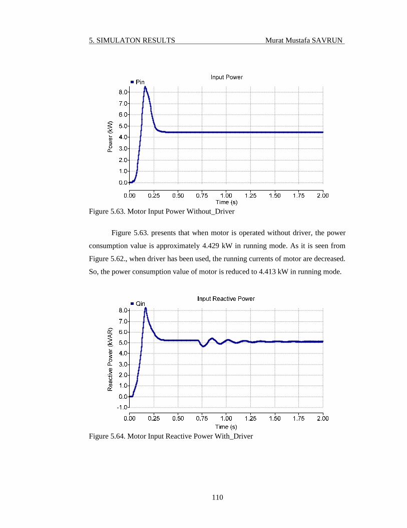
5. SIMULATON RESULTS Murat Mustafa SAVRUN
110
Figure 5.63. Motor Input Power Without_Driver
Figure 5.63. presents that when motor is operated without driver, the power
consumption value is approximately 4.429 kW in running mode. As it is seen from
Figure 5.62., when driver has been used, the running currents of motor are decreased.
So, the power consumption value of motor is reduced to 4.413 kW in running mode.
Figure 5.64. Motor Input Reactive Power With_Driver

5. SIMULATON RESULTS Murat Mustafa SAVRUN
111
Figure 5.65. Motor Input Reactive Power Without_Driver
Figure 5.64. and Figure 5.65. show that reactive power component
(magnetizing current) of motor current is decreased by reducing the stator voltage.
So, the power factor value of motor has been improved for the operation of 50%
torque.
Figure 5.66. Speed of Motor With_Driver

5. SIMULATON RESULTS Murat Mustafa SAVRUN
112
As it is clearly seen from Figure 5.66. – Figure 5.67., although current,
voltage and power values of motor are reduced, the desired motor speed values
remained constant again in the Case 5.
Figure 5.67. Speed of Motor Without_Driver
When the results of Case 5 are examined in detail, figures obviously show
that energy efficiency is obtained from active power and power factor. When motor
is operated without driver, it consumes 4.429 kW. If the driver is used,
approximately 16 W active power is saved and 0.36% energy efficiency is achieved.
Moreover 3% power factor efficiency is also achieved.
5.8. Case 7: Dynamic Performance
The dynamic performance situation of motor is examined in the Case 7. The
motor has been operated in different loads as respectively 0%, 10%, 30%, 20%, 40%,
0%, 10% and 0%. The dynamic performance waveforms are shown in Figure 5.68.
and 5.69.

5. SIMULATON RESULTS Murat Mustafa SAVRUN
113
Figure 5.68. Dynamic Performance With_Driver
Figure 5.69. Dynamic Performance Without_Driver
When the figures examined in detail, it is obviously seen that energy
efficiency is obtained from active power. Energy efficiency in lightly loads is easily
observed from the figures. Efficiency is emphasized more clearly in the Figure 5.70.

5. SIMULATON RESULTS Murat Mustafa SAVRUN
114
Figure 5.70. Comparison of Power Consumption in Dynamic Performance
5.9. Case 8: Short Circuit Performance
The system generally operates in steady state conditions but the characteristic
of the system in the short circuit or abnormal conditions must be known (Teke,
2005). The dynamic short circuit performance of 10 hp induction machine is shown,
respectively in Figure 5.71, 5.72 and 5.73 during a short-circuit fault at the terminals.
Initially the motor is running at steady state conditions with a constant load
torque. The short circuit fault at the terminals is simulated by setting the fault
condition at time t=2 sec. At that instant, the short circuit occurs and causes a high
increase in current and a decrease in voltage. If the peak input current increases, this
increase causes premature diode failure, which may occur within minutes. If rms
input current increases, this increase causes additional heating in the input wiring,
which may result in damage to the installation (Schneider). To prevent this adverse
effects, the under voltage and the over current protections directly start up. The
protections block the operation in 0.1 seconds (see Figure 5.83, 5.84 and 5.8.).

5. SIMULATON RESULTS Murat Mustafa SAVRUN
115
Figure 5.71. Comparison of Power Consumption in Dynamic Performance
Figure 5.72. Comparison of Power Consumption in Dynamic Performance

5. SIMULATON RESULTS Murat Mustafa SAVRUN
116
Figure 5.73. Comparison of Power Consumption in Dynamic Performance

6. CONCLUSION Murat Mustafa SAVRUN
117
6. CONCLUSION
By the day, because of the exponential growth of world population, industrial
developments and the world economy, the energy consumption values of the world is
increasing exponentially. Exhaustible sources not cover the growing energy needs of
the world in the coming years. Hence, world prefers the use of renewable energy
instead of fossil fuels. Besides, the importance that is given to energy efficiency
applications is increasing to use limited energy as more efficient. To use the clean
energy as more efficient, new policies and regulations are determined in Turkey as
well as all over the world.
Industrial sectors are the most energy consuming sector in the world.
Industrial motors use a significant portion of the total industrial energy use. Induction
motors are widely used in industry because of their cost, reliability, robustness and
easy maintenance. Hence, minimizing losses in induction machines would be a major
step towards minimizing the global electric load and energy consumption.
Efficiency of induction machine system improvement activities are divided
into three main directions as machine, power electronics, and control. Such
improvement activities include driver performance, starting methods, induction
motor improved components, and motor loss reduction.
Despite designing the motors for their highest efficiency at the full load,
many industrial induction motors are not operating at full load all the time. In most
instances, motors run under light loads or no load conditions. Typical of such loads
are noncontinuous extruders, conveyors, and some types of fans and compressors
that are constant speed-variable torque applications. In this type of loads that are
been operating in light load operation, a reduction in losses and an improvement in
motor efficiency can be obtained by reducing the stator voltage of the motor.
In this thesis efficiency improvement of lightly load induction motor by
controlling the stator voltage has been examined. Efficiency improvement by stator
flux control is achieved by reducing the applied voltage whenever the torque
requirement of the load can be met with less than full motor flux. Because of

6. CONCLUSION Murat Mustafa SAVRUN
118
reduction in stator flux, the magnetizing component of stator current, core loss and
also copper loss are reduced.
The motor load voltage (stator voltage) is reduced by using thyristor firing
angles according to the torque requirement of the motor. As can be seen from the
Figure 6.1., stator voltage is smaller in with driver operation. The appropriate load
voltage is setting for each torque value. Stator voltage control is performing in 50%
and below loaded conditions, since energy efficiency can be obtained in lightly
loaded operations.
Figure 6.1. Comparison of Load Voltage with and without Driver
The motor load current is reduced by reducing the stator voltage according to
the torque requirement of the motor. As can be seen from the Figure 6.2., load
current is smaller in with driver operation. It means that the motor is consuming
smaller energy with the driver.
100
120
140
160
180
200
220
240
0.0 0.1 0.2 0.3 0.4 0.5
Volta
ge
Torque
Load Voltage
with FLBEC
without FLBEC

6. CONCLUSION Murat Mustafa SAVRUN
119
Figure 6.2. Comparison of Load Current with and without Driver
The total harmonic distortion (THD) of the input current of motor which
operated with the proposed driver as a function of the load is presented in Figure 6.3.
When THD value of the proposed system and THD value of studies in the literature
are compared, it is obviously seen that the proposed system has better THD values.
Figure 6.3. Comparison of Load Current with and without Driver
When the motor current and voltage decrease, the value of motor speed varies
little. It is obviously seen from the Figure 6.4., the motor speed value varies less than
1% that is an acceptable value.
0
2
4
6
8
10
12
0.0 0.1 0.2 0.3 0.4 0.5
Curr
ent
Torque
Load Current
with FLBEC
without FLBEC
0
10
20
30
40
50
60
70
0 0,1 0,2 0,3 0,4 0,5 0,6
THD
%
Motor Load
Total Harmonic Distortion

6. CONCLUSION Murat Mustafa SAVRUN
120
Figure 6.4. Comparison of Motor Speeds with and without Driver
Figure 6.5. Comparison of Power Consumptions with and without Driver
It can be clearly seen from Figure 6.5. and Table 6.1., that when controlled by
driver on lightly loaded conditions, motor can get higher efficiency values. In
conclusion, the presented energy efficiency strategy for 10 hp induction motor brings
a substantial energy savings, particularly at low loads. Proposed driver can be used
for improving the efficiency of electric motors which are constant speed and variably
loaded applications. The driver detects the motor load by using the feedback of
motor speed and delivers the precise amount of energy required by the motor. This
reduces unnecessary energy use. The driver has concluded to save up to 65% of the
energy normally used in appropriate applications.
1200
1250
1300
1350
1400
1450
1500
1550
1600
0.0 0.1 0.2 0.3 0.4 0.5
Spee
d
Torque
Motor Speeds
with FLBEC
without FLBEC
0500
100015002000250030003500400045005000
0 0,05 0,1 0,15 0,2 0,25 0,3 0,4 0,5
Inpu
t Po
wer
(W)
Torque (pu)
Power Efficiency
with FLBEC
without FLBEC

6. CONCLUSION Murat Mustafa SAVRUN
121
Table 6.1. FL Power and Power Factor Efficiency
Proposed driver not only results in a measureable reduction in energy, but
also an improvement in power factor values. In driverless case, due to the large phase
difference between current and voltage, the motor consumes much reactive power. In
driver case, the amount of consumed reactive power is decreased by reducing the
phase difference between current and voltage. So power factor efficiency can be
ensured (see in Figure 6.6. and Table 6.1.).
Figure 6.6. Comparison of Power Factors with and without Driver
The motor power efficiency control with thyristor is not a new topic but not
much work has been reported on it yet. There are only a few theoretical and
simulation studies related about this subject. This study gives some help to literature
Torque Power Efficiency (%) Saved Power (W) PF Efficiency (%)0 65,01 2620,05 29,21 229 92,860,1 17,37 203 66,670,15 11,10 173 46,430,2 7,37 144 31,430,25 4,93 116 21,950,3 3,16 87 14,890,4 1,14 41 7,140,5 0,36 16 3,13
Power Savings & Efficiencies as a Result of Voltage Reduction
0
0,1
0,2
0,3
0,4
0,5
0,6
0,7
0,05 0,1 0,15 0,2 0,25 0,3 0,4 0,5
Pow
er F
acto
r
Torque (pu)
Power Factor Efficiency
with FLBEC
without FLBEC

6. CONCLUSION Murat Mustafa SAVRUN
122
with new controller, and different case studies. The publications made as a result of
this study will also contribute to scientific literature. Further research could be
carried out in the following areas:
§ Performance evaluation of the motor under the different switching
techniques.
§ Investigation and comparison of the efficiency values under the different
topologies of driver.
§ Comparison of the performance of the simulation results and laboratory
application results.

123
REFERENCES
ABB Review. http://library.abb.com/gl obal/scot/scot271.nsf/veritydispla y/131187
a016110b67c12 572ff 0 02faacc/$ File/81-84%202M74 6_ENG72dp i.pdf,
(date of access: 11.05.2012).
AYYUB, M., 2006. ANFIS Based Soft-Starting and Speed Control of AC Voltage
Controller Fed Induction Motor, Power India Conference IEEE,
10.1109/POWERI.2006.1632611.
BAI, Y., HANQUI, Z., 2006. Advanced Fuzzy Logic Technologies in Industrial
Applications: Fundamentals of Fuzzy Logic Control – Fuzzy Sets, Fuzzy
Rules and Defuzzifications. Springer.
BENBOUZID, M. E. H., BEGUENANE, R., CAPOLINO, G. A., 1996. Single-phase
Capacitor Motor Efficiency Improvement by Means of Voltage Control,
Electrotechnical Conference, MELECON '96., 8th Mediterranean IEEE,
Volume: 1, Page(s): 302 – 305, 13-16 May.
BLAABJERG, F., PEDERSON, J. K., RISE, S., HANSEN, H. H.,
TRZYNADLOWSKI, A. M., 1997. Can Soft-Starters Help Save Energy,
IEEE Industry Applicafions Magazine, 1077-2618/97.
CARRIER CORPORATION, 2005. Variable Frequency Drive Operation and
Application of Variable Frequency Drive (VFD) Technology. Carrier
Corporation Syracuse, New York, October.
CHAPMAN, S. J., 1999. Electric Machinery Fundamentals. Third Edition. McGraw-
Hill. Page(s): 357-395.
CUMA, M. U., 2006. Design and Applications of Fuzzy and Neural Controllers.
MSc Thesis. Department of Electrical and Electronics Engineering Çukurova
University.
DA SILVEIRA, E., PIRES, R. C., DE ALMEIDA, A. T. L., JOSE, A., 2009. Direct
on Line Starting Induction Motor with Thyristor Switched Capacitor Based
Voltage Regulation. Power Electronics Conference IEEE, Page(s): 1124 –
1129, Bonito-Mato Grosso do Sul.

124
DAYONG, G., WENGE, M., 2011. Modeling and Simulating for Soft Starting of
Asynchronous Motors Based on Fuzzy Adaptive Control, Intelligent Systems
and Applications (ISA) Conference IEEE, Page(s):1 – 4, 28-29 May, Wuhan.
ELTAMALY, A. M., ALOLAH, A. I., HAMOUDA, R. M., 2007. Performance
Evaluation of Three-Phase Induction Motor under Different AC Voltage
Control Strategies ' Part I', Electrical Machines and Power Electronics,
ACEMP '07. International Aegean Conference IEEE, Page(s): 770 - 774, 10-
12 September, Bodrum.
FUCHS, E. F., HANNA, W. J., 2002. Measured Efficiency Improvements of
Induction Motors With Thyristor/Triac Controllers, IEEE Transactions On
Energy Conversion, Volume: 17, No: 4
FUZZY L.T., (Fuzzy Logic Toolbox), 1995. Fuzzy Logic Toolbox For Use with
MATLAB. The Math Works.
GASTLI, A., AHMED, M. M., 2005. ANN-Based Soft Starting of Voltage-
Controlled-Fed IM Drive System, IEEE Transactions on Energy Conversion,
Volume: 20, No: 3, Page(s): 497 – 503, September.
HRABOVCOVA, V., KALAMEN, L., SEKERAK, P., RAFAJDUS, P., 2010.
Determination of Single Phase Induction Motor Parameters, International
Symposium on Power Electronics Electrical Drives, Automation and Motion
SPEEDAM, IEEE, Page(s): 287 – 292, 14-16 June, Pisa.
HUI, H., XUEDONG, J., RUICHANG, Q., 2005. Simulation and Experiment
Research on 3-Phase Asynchronous Motor Softstarting and Energy-saving
Control, Electrical Machines and Systems, ICEMS, Proceedings of the Eighth
International Conference IEEE, Volume: 2, Page(s): 1595 - 1598, 29
September, Nanjing.
INAAM, I. Starting Method for Induction Motors. http://uotechnology.edu.iq/dep-
eee/lectures/3rd/Communication/machine/PART%202.pdf, (date of access:
11.09.2012).

125
KAI, L., XINGLIN, C., YAN, W., 2005. Analysis of Thyristor Controlled Induction
Motors Based on VVCF, Electrical Machines and Systems, Proceedings of
the Eighth International Conference on ICEMS IEEE, Volume: 1, Page(s):
115 - 118
KAUR, R., BHARDWAJ, M., MALHOTRA, N., 2012. Analyzing Imprecise
Requirements Using Fuzzy Logic. International Journal of Engineering
Research & Technology (IJERT), Volume: 1, Issue: 6, August.
KJELLBERG, M., KLING, S., 2003. Soft Starter Handbook. ABB Automation
Technology Products, February.
LARABEE, J., PELLEGRINO, B., FLICK, B., 2005. Induction Motor Starting
Methods and Issues, Petroleum and Chemical Industry Conference IEEE,
Page(s): 217 – 222, 12-14 September.
LEE, C. C., 1990. Fuzzy Logic in Control Systems: Fuzzy Logic Controller. I.
Systems, Man and Cybernetics, IEEE Transactions, Volume: 20, Page(s):
404 – 418, March/April.
LI, S., LIU, Z., 2009. Constant-Current Soft Starting of Induction Motor Based on
Fuzzy Control, Computer Engineering and Technology, ICCET '09.
International Conference, Volume: 2, Page(s): 358 – 361, 22-24 January
Singapore.
LIPO, T. A., 1971. The Analysis of Induction Motors with Voltage Control by
Symmetrically Triggered Thyristors. Power Apparatus and Systems, IEEE
Transactions, Volume: PAS-90, Page(s): 515 – 525, March.
MCELVEEN, R. F.; TONEY, M. K., 2001. Starting High-Inertia Loads. Industry
Applications, IEEE Transactions, Volume: 37, Page(s): 137 – 144
January/February.
MENDEL, J.M., 1995, Fuzzy Logic Systems for Engineering: A tutorial.
Proceedings of IEEE, 83 (3):345-377.
MISTRY, J. N., SOLANKI, H. D.,, VALA, T. M ., 2012. Variable Frequency Drive.
Research Expo International Multidisciplinary Research Journal, Volume: 2,
Issue: 3, Page(s): 252-256, September.

126
MOHAN, N., 1980. Improvement in Energy Efficiency of Induction Motors by
Means of Voltage Control, IEEE Transactions on Power Apparatus and
Systems, Volume: PAS-99, No: 4.
PAICE, D. A., 1968. Induction Motor Speed Control by Stator Voltage Control,
IEEE Transactions on Power Apparatus and Systems, Volume: PAS-87, No:
2, Page(s): 585 – 590, February.
PATIL, P. S., PORATE, K. B., 2009. Starting Analysis of Induction Motor a
Computer Simulation by Etap Power Station, IEE Computer Society, 978-0-
7695-3884-6/09.
PILLAY, K., NOUR, M., YANG, K. H., HARUN, D. N. D., HAW, L. K., 2009.
Assessment and Comparison of Conventional Motor Starters and Modern
Power Electronic Drives for Induction Motor Starting Characteristics.
Industrial Electronics & Applications, ISIEA-09, IEEE Symposium, Volume:
2, Page(s): 584-589, Kuala Lumpur.
PITIS, C. D., ZELLER, M. W., 2008. Power Savings Obtained from Supply Voltage
Variation on Squirrel Cage Induction Motors, Electric Power Conference,
EPEC IEEE, Page(s): 1 - 3, 6-7 October, Vancouver.
POWER E. (Power Efficiency). Energy Efficiency Technologies for AC Motor.
Power Efficiency Corporation. http://www.powerefficiency.com/ pdf/ ET%20
Summit_S an%20Diego% 202008.pdf, (date of access: 11.05.2012).
RAFEEK, M., JOSE, B. M., NITHIN, K. S., PAUL, B., 2013. A Novel Soft Starter
for Three-Phase Induction Motors with Reduced Starting Current and
Minimized Torque Pulsations. International Journal of Engineering and
Innovative Technology (IJEIT) Volume: 2, Issue: 8, February.
RAJAJI, L., KUMAR, C., VASUDEVAN, M., 2008. Fuzzy and Anfis Based Soft
Starter Fed Induction Motor Drive for High Performance Applications,
ARPN Journal of Engineering and Applied Sciences, Volume:3, No: 4,
August.

127
RANDALL, L., FOULKE, P.E., 2009. Principles and Applications of Variable
Frequency Drives. NC AWWA-WEA Spring Conference April 6, New Bern,
North Carolina.
RASHID, M. H., 2001. Power Electronics Handbook. Academic Press. International
Standard Book Number: 0-12-581650-2, Canada.
ROWAN, T.M., LIPO, T.A., 1983. A Quantitative Analysis of Induction Motor
Performance Improvement by SCR Voltage Control, IEEE Transactions on
Industry Applications, Volume: IA-19, No:4, Page(s): 545 - 553, July/August.
SAIDUR, R., 2010. A Review on Electrical Motors Energy Use and Energy Savings,
Renewable and Sustainable Energy Reviews, 14 (2010) 877–898.
SASTRY, V. V., PRASAD, M. R., SIVAKUMAR, T. V., 1997. Optimal Soft
Starting of Voltage-Controller-Fed IM Drive Based on Voltage Across
Thyristor, IEEE Transactions on Power Electronics, Volume: 12, No: 6,
Page(s): 1041 – 1051, November.
SCHNEIDER. http://static.schneider-electric.us/docs/Motor%20Control/AC % 20D
rives/8800DB0801%20f ile s.pdf (date of access: 27.09.2012).
SIBSON, J., 2012. Using Variable Speed Drives, Servo Motors and RS-485
Communication in a Solar Tracking System for Educational Purposes.
Murdoch University, MSc Thesis, Page(s): 10.
TEKE, A., 2005. Modeling of Dynamic Voltage Restorer. MSc Thesis. Department
of Electrical and Electronics Engineering, Çukurova University.
TEKE, A., MERAL, M. E., SARIBULUT, L., TÜMAY, M., 2011. Implementation
of fuzzy logic controller using FORTRAN language in PSCAD/EMTDC.
International Journal of Electrical Engineering Education, Volume: 48, Issue:
4, p372, October
TOKUOKA, G. A., TOKUOKA, S., 2010. U.S. Adoption of High-Efficiency Motors
and Drives Research. Center on Globalization, Governance &
Competitiveness, Duke University, February.

128
TÖPFER, K. Energy Efficiency Guide for Industry in Asia. http://www.gr
eenbiz.com/sites/default/files/document/CustomO16C45F67124.pdf (date of
access: 13.05.2012).
VERNON, J. Fuzzy Logic Systems. http://www.control-systems-principles
.co.uk/whitepap ers/fuzzy-logic-systems.pdf, (date of access: 27.05.2012).
WIGINGTON, A., 2010. A Comparison of Induction Motor Starting Methods Being
Powered by a Diesel-Generator Set Thesis. Faculty of The Graduate College
at the University of Nebraska, Page: 16.
WILLIAMS, A. J., GRIFFITH, M. S., 1978. Evaluating the Effects of Motor Starting
on Industrial and Commercial Power Systems. Industry Applications, IEEE
Transactions, Volume: IA-14, Page(s): 292 – 305, July.
XIUHE, W., HUI, Z., YUBO, Y., XIAOLEI, M., 2010. Study of a Novel Energy
Efficient Single-Phase Induction Motor With Three Series-Connected
Windings and Two Capacitors. Energy Conversion, IEEE Transactions,
Volume: 25, Page(s): 433 – 440.

129
BIOGRAPHY
Murat Mustafa SAVRUN was born in Osmaniye, Turkey in 1987. He
received his B.S. degree in Electrical and Electronics Engineering Department from
Çukurova University in 2010. After completion his B.S. education, he started MSc
education in Electrical and Electronics Engineering Department in Çukurova
University. He has been working as a Research Assistant in Electrical and
Electronics Engineering Department of the Osmaniye Korkut Ata University since
2010. His research areas are Energy Efficiency, Motor Drives and Power Electronics.