Çukurova university institute of natural applied … · Çukurova university institute of natural...
TRANSCRIPT

ÇUKUROVA UNIVERSITYINSTITUTE OF NATURAL APPLIED SCIENCES
PhD THESIS
Mehmet BİLGİLİ
PREDICTIONS OF WIND SPEED AND WIND POWER POTENTIALUSING ARTIFICIAL NEURAL NETWORKS
DEPARTMENT OF MECHANICAL ENGINEERING
ADANA, 2007

ÇUKUROVA ÜNİVERSİTESİFEN BİLİMLERİ ENSTİTÜSÜ
PREDICTIONS OF WIND SPEED AND WIND POWER POTENTIALUSING ARTIFICIAL NEURAL NETWORKS
Mehmet BİLGİLİ
DOKTORA TEZİ
MAKİNA MÜHENDİSLİĞİ ANABİLİM DALI
Bu tez …/…/2007 Tarihinde Aşağıdaki Jüri Üyeleri Tarafından Oybirliği ile KabulEdilmiştir.
İmza:………………. İmza:……………… İmza:……………………………..Prof.Dr.Beşir ŞAHİN Prof.Dr.Erdem KOÇ Prof.Dr.Ertuğrul BALTACIOĞLUDANIŞMAN ÜYE ÜYE
İmza:…………………… İmza:……………………….Doç.Dr.Hüseyin AKILLI Doç.Dr.Ahmet PINARBAŞIÜYE ÜYE
Bu Tez Enstitümüz Makine Mühendisliği Anabilim Dalında Hazırlanmıştır.Kod No:
Prof. Dr. Aziz ERTUNÇEnstitü Müdürü
İmza Mühür
Bu çalışma Ç. Ü. Araştırma Projeleri Birimi tarafından desteklenmiştir.Proje No: MMF2006D18
Not: Bu tezde kullanılan özgün ve başka kaynaktan yapılan bildirişlerin, çizelge, şekil ve fotoğraflarınkaynak gösterilmeden kullanımı, 5846 sayılı Fikir v Sanat Eserleri Kanunundaki hükümlere tabidir.

I
ABSTRACT
PhD THESIS
PREDICTIONS OF WIND SPEED AND WIND POWER POTENTIALUSING ARTIFICIAL NEURAL NETWORKS
Mehmet BİLGİLİ
DEPARTMENT OF MECHANICAL ENGINEERINGINSTITUTE OF NATURAL APPLIED SCIENCES
ÇUKUROVA UNIVERSITY
Supervisor : Prof.Dr. Beşir ŞAHİN Year : 2007, Pages: 193 Jury : Prof.Dr. Erdem KOÇ Prof.Dr. Ertuğrul BALTACIOĞLU Assoc.Prof.Dr. Hüseyin AKILLI Assoc.Prof.Dr. Ahmet PINARBAŞI
In this study, wind power density in the southern and southwestern region ofTurkey was determined by using the Weibull and Rayleigh probability densityfunctions and the Wind Atlas Analysis and Application Program (WAsP). Moreover,wind speed of a target station was predicted using wind speeds of reference stationsand other meteorological parameters with the artificial neural networks (ANNs)method. ANNs were also applied to predict the long term monthly temperature andrainfall at any specific point of Turkey based on the use of the neighboringmeasuring stations data. The wind data taken with an interval of one hour weremeasured by the General Directorate of Electrical Power Resources SurveyAdministration (EIE) at 9 measuring stations such as Akhisar, Belen, Datça,Gelendost, Söke, Gökçeada, Foca, Gelibolu and Bababurnu. The long-term winddata, containing hourly wind speeds and directions, cover the period from the year1998 to 2003. Wind speeds of reference stations and other meteorological parameterswere used as an input neurons in the ANN architecture, while the target station windspeed was used as an output neuron in the ANN architecture. In MATLAB, differentartificial neural network learning algorithms have been used to establish the ANNmodels. The results obtained with these models were compared with the actual data.Comparisons have shown that there was a good agreement between predicted andmeasured data. Errors obtained in these models are well within acceptable limits.
Keywords: Artificial neural networks, Meteorological parameters, Reference station,Target station, Wind speed.

II
ÖZ
DOKTORA TEZİ
YAPAY SİNİR AĞLARI İLE RÜZGAR HIZI VE RÜZGAR GÜCÜPOTANSİYELİ TAHMİNLERİ
Mehmet BİLGİLİ
ÇUKUROVA ÜNİVERSİTESİFEN BİLİMLERİ ENSTİTÜSÜ
MAKİNA MÜHENDİSLİĞİ ANABİLİM DALI
Danışman : Prof.Dr. Beşir ŞAHİN Yıl : 2007, Sayfa: 193 Jüri : Prof.Dr. Erdem KOÇ Prof.Dr. Ertuğrul BALTACIOĞLU Doç.Dr. Hüseyin AKILLI Doç.Dr. Ahmet PINARBAŞI
Bu çalışmada, Türkiye’nin güney ve güneybatı bölgesindeki rüzgar gücüpotansiyeli, Weibull ve Rayleigh olasılık yoğunluğu fonksiyonları ve “Wind AtlasAnalysis and Application” Programı (WAsP) kullanılarak hesaplanmıştır. Ayrıca, birhedef istasyonun rüzgar hızı, etrafını çevreleyen referans istasyonların rüzgarhızlarından ve diğer meteorolojik parametrelerinden faydalanılarak yapay sinir ağları(YSA) yöntemi ile tahmin edilmiştir. Bundan başka, YSA, Türkiye’nin herhangi birözel noktasındaki ortalama sıcaklık ve yağmur parametrelerini, etrafını çevreleyenreferans istasyonların değerlerinden faydalanarak tahmin etmek için uygulanmıştır.Bir saat aralıklarla alınan rüzgar hızı dataları, Elektrik İşleri Etüt İdaresi (EİE)tarafından Akhisar, Belen, Datça, Gelendost, Söke, Gökçeada, Foca, Gelibolu veBababurnu gibi 9 ayrı rüzgar ölçüm istasyonlarından elde edilmiştir. Saatlik rüzgarhızları ve yön bilgilerini içeren datalar 1998 ile 2003 yılları arasını kapsamaktadır.Referans istasyonlar olarak kabul edilen istasyonların rüzgar hızı dataları ve diğermeteorolojik parametreler oluşturulan yapay sinir ağının giriş katmanındakullanılırken, hedef istasyon olarak kabul edilen istasyonun rüzgar hızı değeri yapaysinir ağının çıkış katmanında kullanılmıştır. MATLAB programında, farklı yapaysinir ağı öğrenme algoritmaları kullanılarak bir tahmin modeli oluşturulmuş ve eldeedilen sonuçlar ile gerçek değerler karşılaştırılmıştır. Bunun sonucunda bulunan hatadeğerlerinin kabul edilebilir sınırlar içerisinde olduğu görülmüştür.
Anahtar Kelimeler: Hedef istasyon, Meteorolojik parametreler, Referans istasyon,Rüzgar hızı, Yapay sinir ağları.

III
ACKNOWLEDGEMENTS
The list is endless if I have to thank all the people that made possible this
work. My first and sincere thanks goes to my advisor Prof. Dr. Beşir ŞAHİN for his
support, guidance and encouragement. He showed me what I thought nobody could
really do: that there are no limits on what we can achieve. Thanks, from the bottom
of my heart.
I would like to thank Prof. Dr. Erdem KOÇ for his technical support,
guidance, and dedication throughout the preparation of this thesis. Knowing and
feeling his support during my PhD thesis helped me a lot to my self-confidence.
I am grateful to Assist. Prof. Dr. Hüseyin AKILLI for his continues support,
help, friendship and encouragement.
On a personal level many thanks go to Lecturer Yılmaz KOÇAK, Erdoğan
ŞİMŞEK and Yusuf POLAT for their continuous moral support, motivation and
friendship.
In addition, I would like to thank all the staff of Department of Mechanical
Engineering at Çukurova University.
At last, but not least, I would like to thank my wife, Ferhunde. Finally, I
would like to thank my daughter and son.

IV
NOMENCLATURE
EIE : Elektrik İşleri Etüd İdaresi
IEA : International Energy Agency
TEK : Türkiye Elektrik Kurumu
MENR : Ministry of Energy and Natural Sources (Enerji ve Tabii
Kaynaklar Bakanlığı)
TEAS : Türkiye Elektrik Üretim-Iletim A.S.
TEDAS : Türkiye Elektrik Dagitim A.S.
TEIAS : Turkiye Elektrik Iletim A.S.
EUAS : Elektrik Uretim A.S.
EPDK : Enerji Piyasasi Duzenleme Kurumu
MTA : Maden Tetkik ve Arama
BOTAŞ : Boru Hatları ile Petrol Taşıma A.Ş.
ANN : Artificial Neural Network
SCG : Scaled Conjugate Gradient
LM : Levenberg-Marquardt
CGP : Pola-Ribiere Conjugate Gradient
RBFN : Radial Basis Function Network
HFM : Hopfield Model
MLP : Multi-Layered Perceptron
ERNN : Elman Recurrent Neural Network
SCCF : Sample Cross Correlation Function
ARMA : Aautoregressive moving average
ANFIS : Adaptive Neuro-Fuzzy Inference Systems
SVM : Support Vector Machines
PCA : Principal Component Analysis
WAsP : Wind Atlas Analysis and Application Program
TSMS : Turkish State Meteorological Service
LMS : Least Mean Square
RP : Resilient Propagation

V
MLR : Multiple Linear Regression
RPE : Recursive Prediction Error
RMSE : Root Mean Squared Error
MAPE : Mean Absolute Percentage Error
MAE : Mean Absolute Error
RSP : Respirable Suspended Particulates
MATLAB : Matris Laboratuarı
GWh : Gigawatt hour
GW : Gigawaat
MW : Megawatt
p : Total number of inputs
y : Input signals
w : Synaptic weights
u : Linear combiner output
q : Threshold
(.)j : Activation function
f(x) : Transfer function
n : Iteration number
d(n) : Desired response or target output
e(n) : Error signal
y(n) : Function signal appearing at the output of neuron
E(n) : Instantaneous sum of squared errors of the network
v(n) : Net internal activity level
( )jiw nD : Correction
( ) / ( )jiE n w n¶ ¶ : Instantaneous gradient
h : Learning-rate parameter
( )j nd : Local gradient
a : Unknown coefficient
y : Dependent value
x : Independent value

VI
A : Area (m2)
c : Weibull scale parameter (m/s)
f(v) : Probability of measured wind speed
fW(v) : Weibull probability function
fR(v) : Rayleigh probability function
FW(v) : Cumulative Weibull probability function
FR(v) : Cumulative Rayleigh probability function
k : Weibull shape parameter (dimensionless)
n : Number of observations
P(v) : Mean wind power density (W/m2)
PW : Weibull mean wind power density (W/m2)
PR : Rayleigh mean wind power density (W/m2)
R : Correlation coefficient
v : Wind speed (m/s)
vm : Mean wind speed (m/s)
()G : Gamma function
r : Air density (kg/m3)
s : Standard deviation (m/s)

VII
TABLE OF CONTENTS PAGE
ABSTRACT……………………………………………………………………. I
ÖZ………………………………………………………………………………. II
ACKNOWLEDGEMENT…………………………………………………...… III
NOMENCLATURE……………………………………………………………. IV
TABLE OF CONTENTS………………………………………………………. VII
LIST OF TABLES……………………………………………………………... X
LIST OF FIGURES ……………………………………………………………. XII
1. INTRODUCTION…………………………………………………………… 1
1.1. Development of Electricity Generation in Turkey…………………….. 2
1.2. Energy Resources in Turkey’s Electricity Generation………………… 5
1.3. Thermal Power Plants in Turkey………………………………………. 8
1.4. Hydro Power Plants in Turkey………………………………………… 12
1.5. Wind Power Plants in Turkey…………………………………………. 17
1.6. Geothermal Power Plants in Turkey…………………………………... 20
1.7. Aim and Outline of the Study…………………………………………. 22
2. LITERATURE SURVEY…………………………………………………… 27
3. MATERIAL AND METHOD………………………………………………. 35
3.1. Artificial Neural Networks…………………………………………….. 35
3.1.1. Biological and Artificial Neurons………………………………. 35
3.1.2. Models of a Neuron……………………………………………... 37
3.1.3. Types of Transfer Function ……………………...…………… 38
3.1.4. Derivation of the Back-Propagation Algorithm ………….…….. 41
3.1.5. Basic Learning Laws……………………………………………. 48
3.1.5.1. Hebb's Rule………………………………………………... 48
3.1.5.2. Hopfield Law……………………………………………… 49
3.1.5.3. The Delta Rule…………………………………………….. 49
3.1.5.4. The Gradient Descent Rule……………………………….. 49
3.1.5.5. Kohonen's Learning Law………………………………….. 50
3.1.6. Training Algorithms……………………………………………… 50

VIII
3.1.6.1. Resilient Back-propagation (trainrp)………………………. 51
3.1.6.2. Scaled Conjugate Gradient (trainscg)……………………… 52
3.1.6.3. Levenberg-Marquardt (trainlm)……………………………. 52
3.1.7. Benefits of Neural Networks in This Study…………………….. 52
3.1.8. Computer Program Used in MATLAB…………………………. 54
3.2. Multiple Linear Regression Analysis…………………….……………. 55
3.3. WAsP Program……………………………………………………….... 56
3.4. Weibull and Rayleigh Distribution Function………………………….. 57
4. RESULTS AND DISCUSSIONS…………………………………………… 61
4.1. Wind Power Potential of the Eastern Mediterranean Region of Turkey. 61
4.1.1. Wind data…..……………………………………………………. 61
4.1.2. The Results of Corrected Values of Wind Data…………………. 74
4.2. Wind Characteristics in Belen-Hatay, Turkey………………………… 76
4.2.1. Location of the Site……………………………………………… 76
4.2.2. Wind Speed Probability Distribution……………………………. 78
4.2.3. Wind Direction Frequency Distribution…………………………. 80
4.2.4. Variation of Weibull Parameters………………………………… 81
4.2.5. Variation of Wind Speeds……………………………………….. 83
4.2.6. Variation of Wind Power Potential……………………………… 87
4.3. Investigation of Wind Power Density in the Southern and
Southwestern Region of Turkey……………………………………….. 91
4.3.1. Location of the Sites……………………………………………... 91
4.3.2. Wind Data Analysis …………………………………………….. 92
4.3.3. Probability Density Distributions ……………………………….. 97
4.3.4. Power Density Distributions…………………………………….. 101
4.4. Prediction of Wind Power Potential …………………………………. 106
4.4.1. Preparation of Input and Output Data…………………………… 106
4.4.2. Artificial Neural Network Architecture…………………………. 108
4.4.3. Results and Discussion………………………………………….. 110
4.5. Application of Artificial Neural Networks for the Wind Speed
Prediction of Target Station Using Reference Stations Data………….. 117

IX
4.5.1. Preparation of Input and Output Data……..…………………….. 117
4.5.2. Artificial Neural Network Architecture……..…………………... 120
4.5.3. Results and Discussion…………………………………………... 122
4.6. Wind Speed Prediction Using Other Meteorological Variables………. 127
4.6.1. Analysis of meteorological variables……………………………. 128
4.6.2. Results for Multiple Regression Analysis……………………….. 133
4.6.3. Results for Artificial Neural Networks………………………….. 136
4.6.4. Comparative Analysis of MLR model to ANN model………….. 139
4.7. Daily, Weekly and Monthly Wind Speed Predictions of Target Station
Using Artificial Neural Networks……………………………………... 141
4.7.1. Preparation of Input and Output Data…………………………… 141
4.7.2. Application………………………………………………………. 144
4.7.2.1. Daily Prediction…………………………………………..... 145
4.7.2.2. Weekly Prediction………………………………………..... 149
4.7.2.3. Monthly Prediction………………………………………… 152
4.7.3. Results and Discussion………………………………………….. 155
4.8. Prediction of Long Term Monthly Temperature and Rainfall in Turkey
Using Artificial Neural Networks……………………………………... 159
4.8.1. Data Analysis and Climate of Turkey…………………………… 159
4.8.2. Artificial Neural Network Architecture…………………………. 165
4.8.3. Results and Discussion…………………………………………... 167
5. CONCLUSIONS AND RECOMMENDATIONS…………………………... 181
ACKNOWLEDGEMENT………………………………………………….. 185
REFERENCES…………………………………………………………………. 186
CIRRUCULUM VITAE………………………………………………….……. 193

X
LIST OF TABLES PAGE
Table 1.1. Turkey’s thermal electric capacity by the electricity utilities…. 9
Table 1.2. Thermal power plants of the EUAS, affiliated partnerships of
EUAS and private entities in Turkey………………………….. 10
Table 1.2. (Continued) Thermal power plants of the EUAS, affiliated
partnerships of EUAS and private entities in Turkey…………. 11
Table 1.3. Turkey’s hydro electric capacity by the electricity utilities in
2005……………………………………………………………. 13
Table 1.4. Hydro power plants with dam of the EUAS in Turkey………... 15
Table 1.4. (Continued) Hydro power plants with dam of the EUAS in
Turkey………………………………………………………… 16
Table 1.5. Potential of hydro power plants in Turkey as of February 2007. 17
Table 1.6. Distribution of Turkey’s wind energy installations by regional
as of May 2007 (*: In operation, others: Under construction)… 19
Table 1.7. Geothermal power plants in Turkey…………………………… 22
Table 3.1. Transfer functions and graphs…………………………………. 39
Table 3.1. (Continued) Transfer functions and graphs……………………. 40
Table 3.2. Training algorithms……………………………………………. 51
Table 4.1. Locations of stations…………………………………………… 61
Table 4.2. The sectoral frequencies of wind direction at meteorological
stations…………………………………………………………. 64
Table 4.3. Hourly wind data at meteorological stations…………………... 64
Table 4.4. Geographical coordinate and measurement period of Belen
station………………………………………………………….. 78
Table 4.5. The Weibull parameters according to the wind directions…….. 82
Table 4.6. The monthly Weibull parameters……………………………… 83
Table 4.7. The yearly mean wind characteristics measured in the year of
2004 and 2005…………………………………………………. 90
Table 4.8. Geographical coordinates and measurement years of stations… 92
Table 4.9. Monthly and annual mean wind speed and standard deviation

XI
for all stations………………………………………………….. 95
Table 4.10. Monthly and annual Weibull parameters for all stations………. 96
Table 4.11. Weibull, Rayleigh and measured probability distribution of the
wind speeds in Belen for the year 2005……………………….. 100
Table 4.12. Performance values for all stations…………………………….. 104
Table 4.13. Annual wind power potentials (W/m2) for all stations………… 105
Table 4.14. Frequency values used in the input layer of the network for
Karataş (year 2000)…………………………………………… 107
Table 4.15. Mean wind power potential used in the output layer of the
network for Karataş (year 2000)……………………………….. 108
Table 4.16. The number of neurons in each layer of network……………… 109
Table 4.17. Statistical errors for different learning algorithms…………….. 111
Table 4.18. Mean wind speeds and dominant prevailing wind directions of
all stations……………………………………………………… 118
Table 4.19. Correlation coefficients of wind speeds amongst stations……. 119
Table 4.20. Reference stations and number of neurons in the hidden layers
of the network for target stations………………………………. 122
Table 4.21. The performance values for training and testing procedure…… 123
Table 4.22. Correlation coefficients between all meteorological variables
for Antakya meteorological station……………………………. 132
Table 4.23. Correlation coefficients between all meteorological variables
for Mersin meteorological station……………………………... 133
Table 4.24. Correlation coefficients between all meteorological variables
for Samandağ meteorological station………………………….. 133
Table 4.25. Performance values of prediction results for all stations………. 140
Table 4.26. Geographical coordinates and measurement periods of stations. 142
Table 4.27. The annual average wind speed, energy potential and dominant
wind direction of stations in 2001……………………………... 144

XII
Table 4.28. Correlation coefficients of daily wind speeds between stations.. 146
Table 4.29. Correlation coefficients of weekly wind speeds between
stations…………………………………………………………. 149
Table 4.30. Correlation coefficients of monthly wind speeds between
stations…………………………………………………………. 152
Table 4.31. The performance values for learning and testing process
a) For daily wind speeds………………………………….......... 156
Table 4.31. (Continued) The performance values for learning and testing
process b) For weekly wind speeds……………………………. 157
Table 4.31. (Continued) The performance values for learning and testing
process c) For monthly wind speeds…………………………... 158
Table 4.32. Geographical coordinates of the stations selected for training
data…………………………………………………………….. 162
Table 4.32. (Continued) Geographical coordinates of the stations selected
for training data………………………………………………... 163
Table 4.32. (Continued) Geographical coordinates of the stations selected
for training data………………………………………………... 164
Table 4.33. Geographical coordinates of the stations selected for testing
data…………………………………………………………….. 164
Table 4.34. The performance values for training procedure……………….. 169
Table 4.34. (Continued) The performance values for training procedure….. 170
Table 4.34. (Continued) The performance values for training procedure….. 171
Table 4.35. The performance values for testing procedure………………… 171

XIII
LIST OF FIGURES PAGES
Figure 1.1. The development of Turkey’s installed capacity in electricity
generation between 1923 and 2005…………………………… 3
Figure 1.2. The development of Turkey’s electricity generation between
1923 and 2005………………………………………………… 4
Figure 1.3. The installed capacity and annual electricity production of
Turkey’s electric power plants in 2005……………………….. 5
Figure 1.4. The development of Turkey’s electricity generation by
primary energy resources between 1940 and 2005…………… 6
Figure 1.5. Turkey’s electricity generation by primary energy resources in
2004 and 2005………………………………………………… 7
Figure 1.6. Locations of thermal power plants of the EUAS, affiliated
partnerships of the EUAS and private entities in Turkey……... 9
Figure 1.7. Turkey’s electricity generation by thermal energy resources in
2004 and 2005………………………………………………… 12
Figure 1.8. Locations of hydro power plants with dam of the EUAS in
Turkey…………………………………………………………. 14
Figure 1.9. Locations of wind power plants in Turkey……………………. 18
Figure 1.10. The development of Turkey’s installed capacity and electricity
generation in the geothermal power plants……………………. 21
Figure 1.11. Locations of geothermal power plants in Turkey……………... 21
Figure 3.1. A simplified model of a biological neuron……………………. 36
Figure 3.2. A simplified model of an artificial neuron……………………. 36
Figure 3.3. Nonlinear model of a neuron………………………………….. 37
Figure 3.4. Signal-flow graph highlighting the details of output neuron j… 41
Figure 3.5. Signal-flow graph highlighting the details of output neuron k
connected to hidden neuron j………………………………….. 45
Figure 4.1. The map of the region, location and dominant wind direction
of the stations…………………………………………………. 62

XIV
Figure 4.2. Topographical map of the region……………………………… 63
Figure 4.3. Frequency distribution of wind speeds for Antakya
meteorological station ………………………………………… 65
Figure 4.4. Frequency distribution of wind speeds for İskenderun
meteorological station…………………………………………. 65
Figure 4.5. Frequency distribution of wind speeds for Dörtyol
meteorological station…………………………………………. 66
Figure 4.6. Frequency distribution of wind speeds for Yumurtalık
meteorological station…………………………………………. 66
Figure 4.7. Frequency distribution of wind speeds for Adana
meteorological station…………………………………………. 67
Figure 4.8. Frequency distribution of wind speeds for Karataş
meteorological station…………………………………………. 67
Figure 4.9. Frequency distribution of wind speeds for Samandağ
meteorological station…………………………………………. 68
Figure 4.10. Daily time variation of the mean hourly wind speeds for
meteorological stations…………………………………… …. 68
Figure 4.11. Variation of the yearly mean wind speeds for meteorological
stations………………………………………………………… 69
Figure 4.12. Monthly variation of mean wind speeds for Antakya
meteorological station…………………………………………. 70
Figure 4.13. Monthly variation of mean wind speeds for İskenderun
meteorological station…………………………………………. 71
Figure 4.14. Monthly variation of mean wind speeds for Dörtyol
meteorological station…………………………………………. 71
Figure 4.15. Monthly variation of mean wind speeds for Karataş
meteorological station…………………………………………. 72
Figure 4.16. Monthly variation of mean wind speeds for Yumurtalık
meteorological station…………………………………………. 72
Figure 4.17. Monthly variation of mean wind speeds for Samandağ

XV
meteorological station…………………………………………. 73
Figure 4.18. Monthly variation of mean wind speeds for Adana
meteorological station…………………………………………. 73
Figure 4.19. Regional distribution of mean wind energy potential (W/m2)
in the south-east region of Mediterranean for 10 m above the
ground level (minimum contour: 250 W/m2, increment: 250
W/m2)………………………………………………………….. 75
Figure 4.20. Regional distribution of mean wind energy potential (W/m2)
in the south-east region of Mediterranean for 25 m above the
ground level (minimum contour: 500 W/m2, increment: 250
W/m2)………………………………………………………….. 76
Figure 4.21. The map of the region and the location of the station………… 77
Figure 4.22. Yearly cumulative probability distributions of wind speeds….. 79
Figure 4.23. Seasonal cumulative probability distributions of wind speeds
for the year 2004………………………………………………. 80
Figure 4.24. Yearly wind direction frequency distribution…………………. 81
Figure 4.25. Seasonal wind direction frequency distribution for the year
2004…………………………………………………………… 81
Figure 4.26. The variation of yearly mean wind speeds according to the
wind directions………………………………………………... 85
Figure 4.27. The variation of seasonal mean wind speeds according to the
wind directions for the year 2004……………………………... 85
Figure 4.28. The monthly variation of mean wind speeds for the year 2004
and 2005………………………………………………………. 86
Figure 4.29. The variation of diurnal wind speeds for the year 2004 and
2005…………………………………………………………… 86
Figure 4.30. The variation of diurnal mean wind speeds for the seasons in
the year 2005………………………………………………….. 87
Figure 4.31. The variation of yearly mean wind power potential according
to the wind directions…………………………………………. 88

XVI
Figure 4.32. The variation of seasonal mean wind power potential for the
year 2004……………………………………………………… 88
Figure 4.33. The monthly variation of mean wind power potential for the
year 2004 and 2005…………………………………………… 89
Figure 4.34. The variation of diurnal wind power potential for the year
2004 and 2005………………………………………………… 89
Figure 4.35. Map of the region and location of the stations………………... 91
Figure 4.36. Wind direction frequency distributions of the stations……….. 93
Figure 4.37. Hourly variation of the mean wind speed……………………... 94
Figure 4.38. Wind speed frequency distributions in Belen station………… 97
Figure 4.39. Wind speed frequency distributions in Datça station…………. 98
Figure 4.40. Wind speed frequency distributions in Foca station…………... 98
Figure 4.41. Wind speed frequency distributions in Gelendost station…….. 99
Figure 4.42. Wind speed frequency distributions in Söke station………….. 99
Figure 4.43. Weibull cumulative probability distributions for all stations…. 101
Figure 4.44. Monthly variation of the mean power densities in Belen……... 102
Figure 4.45. Monthly variation of the mean power densities in Datça……... 102
Figure 4.46. Monthly variation of the mean power densities in Foca……… 103
Figure 4.47. Monthly variation of the mean power densities in Gelendost… 103
Figure 4.48. Monthly variation of the mean power densities in Söke……… 104
Figure 4.49. Annual wind power density distribution obtained from theWeibull model for all stations…………………………………
105
Figure 4.50. Frequency distribution of wind speeds for Karataş (February
2000)…………………………………………………………... 106
Figure 4.51. ANN architecture……………………………………………… 109
Figure 4.52. Comparison between prediction of artificial neural network
(RP, SCG and LM) and actual results for Antakya
meteorological station…………………………………………. 112
Figure 4.53. Comparison between prediction of artificial neural network
(RP, SCG and LM) and actual results for Karataş
meteorological station…………………………………………. 113

XVII
Figure 4.54. Comparison between prediction of artificial neural network
(RP, SCG and LM) and actual results for İskenderun
meteorological station…………………………………………. 113
Figure 4.55. Comparison between prediction of artificial neural network
(RP, SCG and LM) and actual results for Samandağ
meteorological station…………………………………………. 114
Figure 4.56. Actual mean wind power potentials and network predictions
for testing process of Antakya meteorological station………... 114
Figure 4.57. Actual mean wind power potentials and network predictions
for testing process of Karataş meteorological station…………. 115
Figure 4.58. Actual mean wind power potentials and network predictions
for testing process of İskenderun meteorological station……... 115
Figure 4.59. Actual mean wind power potentials and network predictions
for testing process of Samandağ meteorological station……… 116
Figure 4.60. Map of the region, location of the stations and dominant wind
directions……………………………………………………… 118
Figure 4.61. ANN architecture……………………………………………… 121
Figure 4.62. Comparison between prediction of ANN and actual results for
Antakya meteorological station……………………………….. 124
Figure 4.63. Comparison between prediction of ANN and actual results for
İskenderun meteorological station…………………………….. 125
Figure 4.64. Comparison between prediction of ANN and actual results for
Karataş meteorological station………………………………... 125
Figure 4.65. Comparison between prediction of ANN and actual results for
Mersin meteorological station………………………………… 126
Figure 4.66. Comparison between prediction of ANN and actual results for
Samandağ meteorological station……………………………... 126
Figure 4.67. Comparison between prediction of ANN and actual results for
Yumurtalık meteorological station……………………………. 127
Figure 4.68. Average monthly variation of meteorological parameters for
Antakya meteorological station……………………………….. 130

XVIII
Figure 4.69. Average monthly variation of meteorological parameters for
Mersin meteorological station………………………………… 130
Figure 4.70. Average monthly variation of meteorological parameters for
Samandağ meteorological station……………………………... 131
Figure 4.71. Comparison between prediction of MLR and actual results for
Antakya meteorological station……………………………….. 135
Figure 4.72. Comparison between prediction of MLR and actual results for
Mersin meteorological station………………………………… 135
Figure 4.73. Comparison between prediction of MLR and actual results for
Samandağ meteorological station…………………………….. 136
Figure 4.74. ANN architecture……………………………………………… 137
Figure 4.75. Comparison between prediction of RP and actual results for
Antakya meteorological station……………………………….. 138
Figure 4.76. Comparison between prediction of RP and actual results for
Mersin meteorological station………………………………… 138
Figure 4.77. Comparison between prediction of RP and actual results for
Samandağ meteorological station……………………………... 139
Figure 4.78. The map of the region and the location of the stations……….. 142
Figure 4.79. Monthly average wind speed of stations……………………… 144
Figure 4.80. Artificial Neural Network architecture………………………... 145
Figure 4.81. Comparison between predictions of ANN and daily measured
wind speeds for Gökçeada station…………………………….. 147
Figure 4.82. Comparison between predictions of ANN and daily measured
wind speeds for Foca station………………………………….. 147
Figure 4.83. Comparison between predictions of ANN and daily measured
wind speeds for Gelibolu station……………………………… 148
Figure 4.84. Comparison between predictions of ANN and daily measured
wind speeds for Bababurnu station……………………………. 148
Figure 4.85. Comparison between predictions of ANN and weekly
measured wind speeds for Gökçeada station………………….. 150
Figure 4.86. Comparison between predictions of ANN and weekly

XIX
measured wind speeds for Foca station……………………….. 150
Figure 4.87. Comparison between predictions of ANN and weekly
measured wind speeds for Gelibolu station…………………… 151
Figure 4.88. Comparison between predictions of ANN and weekly
measured wind speeds for Bababurnu station………………… 151
Figure 4.89. Comparison between predictions of ANN and monthly
measured wind speeds for Gökçeada station………………….. 153
Figure 4.90. Comparison between predictions of ANN and monthly
measured wind speeds for Foca station……………………….. 153
Figure 4.91. Comparison between predictions of ANN and monthly
measured wind speeds for Gelibolu station…………………… 154
Figure 4.92. Comparison between predictions of ANN and monthly
measured wind speeds for Bababurnu station………………… 154
Figure 4.93. Locations of the measuring stations (○: stations used in
training, ●: stations used in testing)…………………………… 161
Figure 4.94. Long term monthly temperature and rainfall of Turkey………. 161
Figure 4.95. ANN architecture……………………………………………… 166
Figure 4.96. Comparison between prediction of ANN and actual results for
Adana meteorological station…………………………………. 172
Figure 4.97. Comparison between prediction of ANN and actual results for
Adıyaman meteorological station……………………………... 172
Figure 4.98. Comparison between prediction of ANN and actual results for
Amasya meteorological station……………………………….. 173
Figure 4.99. Comparison between prediction of ANN and actual results for
Aydın meteorological station………………………………….. 173
Figure 4.100. Comparison between prediction of ANN and actual results for
Balıkesir meteorological station………………………………. 174
Figure 4.101. Comparison between prediction of ANN and actual results for
Bingöl meteorological station…………………………………. 174
Figure 4.102. Comparison between prediction of ANN and actual results for
Burdur meteorological station………………………………… 175

XX
Figure 4.103. Comparison between prediction of ANN and actual results for
Erzincan meteorological station………………………………. 175
Figure 4.104. Comparison between prediction of ANN and actual results for
Karaman meteorological station………………………………. 176
Figure 4.105. Comparison between prediction of ANN and actual results for
Kars meteorological station…………………………………… 176
Figure 4.106. Comparison between prediction of ANN and actual results for
Kırıkkale meteorological station……………………………… 177
Figure 4.107. Comparison between prediction of ANN and actual results for
Kütahya meteorological station……………………………….. 177
Figure 4.108. Comparison between prediction of ANN and actual results for
Mardin meteorological station………………………………… 178
Figure 4.109. Comparison between prediction of ANN and actual results for
Nevşehir meteorological station………………………………. 178
Figure 4.110. Comparison between prediction of ANN and actual results for
Sakarya meteorological station………………………………... 179
Figure 4.111. Comparison between prediction of ANN and actual results for
Tekirdağ meteorological station………………………………. 179
Figure 4.112. Comparison between prediction of ANN and actual results for
Trabzon meteorological station……………………………….. 180

1. INTRODUCTION Mehmet BİLGİLİ
1
1. INTRODUCTION
Turkey’s geographical location stands as a natural land bridge connecting
Europe to Asia. Therefore, it has increasingly important role to play as an “energy
corridor” between the major oil and natural gas producing countries in the Middle
East, Caspian Sea and the Western energy markets (IEA, 2005). Furthermore,
Turkey, with a population of 65,311,000 in the year of 2000, has the highest
population increasing rate, 1.4% among the Organization for the Economic
Cooperation and Development (OECD) countries. In addition, Turkey’s energy
demand grows rapidly due to the social and economic development of the country
and is expected to continue to grow in the near future (Kaya, 2006).
Energy is one of the most significant components in the economic
development of countries. It is also certain that energy is the most important
necessity of human life and hence there is an increasing relation between the level of
development and amount of energy consumption. It is inevitably essential for the
economic and social growths and an improved quality of life in Turkey, as in other
countries. This situation makes energy resources significantly important for the
whole world (Yılmaz and Uslu, 2007; Sözen and Arcaklıoğlu, 2007). Out of various
energy sources, an electric power is considered to be a kind of energy source which
can be used in variety of industry. In general, electricity is generated from the
hydropower, thermal and nuclear power plants. It is known that the hydropower
plants generate electricity by using generators driven by water turbines, operating by
means of falling water from a certain elevation with a high rate of volume flow rate.
Coal, oil or natural gas are used in the thermal power plants for generating
electricity. Atomic fuels like uranium, thorium and plutonium are used in nuclear
power plants. Other types energy production sources are wind, wave, sun and
biomass (Demirbaş and Bakış, 2004). Supplies of energy resources such as fossil
fuels (coal, oil, natural gas) and nuclear fuels (uranium and thorium) are generally
known to be finite; but other energy sources, such as solar, hydro, biomass, and wind
energies, are generally considered to be renewable and therefore sustainable over the

1. INTRODUCTION Mehmet BİLGİLİ
2
relatively long term. In addition, energy generation from the fossil fuels burned in the
thermal power plants causes to pollutions in the environment (Demirbaş, 2002).
A rapid increase of energy demand in the world is due to the rate of
population growth, the high rate of industrialization, social and economical
development of Turkey. But, thermal power plants based on fossil fuels degrade the
quality of environment in large scale in fact; there is growing evidence of
environmental problems due to a combination of several factors. The environmental
impact of human activities worldwide has also grown dramatically because of the
rate of world population growth, social development, energy consumption,
improving condition of life, industrial activities, etc. Demirbaş (2002) stated that
achieving solutions to the environmental problems that we face today requires long-
term potential actions for sustainable development. In this regard, renewable energy
resources appear to be one of the most efficient and effective solutions.
1.1. Development of Electricity Generation in Turkey
Turkey is located between Europe and Asia. It is situated in Anatolia and
southeastern Europe bordering the Black Sea, the Aegean Sea and the Mediterranean
Sea. Turkey extends more than 1,600 kilometers from west to east but generally less
than 800 kilometers from north to south. Its total land area is about 779,452 square
kilometers, of which 755,688 square kilometers are in Asia and 23,764 square
kilometers in Europe. From the point of view of this geographical location, Turkey is
situated bridge-like between southeastern Europe and Asia. Moreover, the economy
and population of Turkey grow rapidly. As a developing country, Turkey’s
population is estimated to be over 100 million by the year of 2020 (Yüksek et al.,
2006). For this reason, demands for energy and particularly for electricity have been
growing rapidly. Electricity energy is a vital input for the technological, social and
economic development of Turkey (Hamzaçebi, 2007).
Electricity in Turkey is generated from the thermal, hydro, wind and the
geothermal power plants. The development of Turkey’s installed capacity in
electricity generation between 1923 and 2005 is illustrated in Figure 1.1. In addition,

1. INTRODUCTION Mehmet BİLGİLİ
3
the development of Turkey’s electricity generation between 1923 and 2005 is
presented in Figure 1.2. Turkey’s electricity supply industry dates back to 1902,
when a 2 kW dynamo was connected to a water mill in Tarsus. Although this power
plant was the first experience of Turkey in electricity production, the first larger-
scale power plant was built in Istanbul in 1913. When the Republic of Turkey was
founded in 1923, its installed capacity of electricity production and total electricity
production were 33 MW and 45 GWh, respectively (IEA, 2001; Yılmaz and Uslu,
2007). In 1935, the Electrical Power Resources Survey and Development
Administration (Elektrik Isleri Etut Idaresi, EIE) was established for the purpose of
carrying out surveys and preparatory work to assess hydro potential and prepare a
hydro power plant projects. Construction of power plants began on a larger scale, by
both private and publicly-owned entities in the 1950s. At the beginning of the
decade, installed capacity was about 408 MW (IEA, 2001).
010000
200003000040000
50000600007000080000
1923 1933 1943 1953 1963 1973 1983 1993 2003
Year
Inst
alle
d ca
paci
ty (M
W)
Thermal Hydro Total
Figure 1.1. The development of Turkey’s installed capacity in electricity generation between 1923 and 2005
By 1970, installed capacity of electricity was increased to about 2,235 MW,
and both growing power consumption and the government’s electrification plans
required more coherent organization of the power industry. At the time, only 7% of
all villages were electrified. As a consequence, the government established the

1. INTRODUCTION Mehmet BİLGİLİ
4
Turkish Electricity Authority (Türkiye Elektrik Kurumu, TEK) as a fully state-owned
and state run entity that year. In 1993, TEK was split into 2 separate state-owned
electric companies called as the Ministry of Energy and Natural Sources (MENR):
The Turkish Electricity Generation Transmission Corporation (Türkiye Elektrik
Üretim-Iletim A.S., TEAS) and Turkish Electricity Distribution Corporation
(Türkiye Elektrik Dagitim A.S., TEDAS). In 1999, Turkey’s installed power
generation capacity reached 26,117 MW, and 99.9% of its population was connected
to the electricity grid (IEA, 2001; Kıncay and Ozturk, 2003).
0
50000
100000
150000
200000
250000
300000
350000
1923 1933 1943 1953 1963 1973 1983 1993 2003
Year
Elec
tric
ity g
ener
atio
n (G
Wh)
Thermal Hydro Total
Figure 1.2. The development of Turkey’s electricity generation between 1923 and 2005
Figure 1.3 shows the installed capacity and annual electricity production of
Turkey’s electric power plants in 2005. As reported by the Turkish Electricity
Transmission Company (Turkiye Elektrik Iletim A.S., TEIAS), the installed capacity
of Turkey’s electric power plants was 38,843.5 MW with the annual electricity
production of 161,956.2 GWh in 2005 (TEIAS, 2005). Of the total electricity
generation, 75.48% came from the thermal power plants, while 24.43% came from
the hydro power plants. In addition, the wind power plants and the geothermal power
plants met 0.04% and 0.06% of Turkey’s electric power generation, respectively. In
this year, 122,242.3 GWh of this energy was produced by operating the thermal
power plants. On the other hand, the annual electricity productions of the hydro

1. INTRODUCTION Mehmet BİLGİLİ
5
power plants and the wind power plants were 39,560.5 GWh and 59 GWh,
respectively. During the next 20 years, the electric power plants installed capacity is
expected to reach 109,227 MW and the annual electricity production is going to be
623,835 GWh (Kenisarin et al., 2006).
0
20000
40000
60000
80000
100000
120000
140000
Elec
tric
cap
acity
Thermal Hydro Wind Geothermal
Installed capacity (MW)
Annual production (GWh)
Figure 1.3. The installed capacity and annual electricity production of Turkey’s electric power plants in 2005
1.2. Energy Resources in Turkey’s Electricity Generation
The demand for energy in the world grows rapidly and is expected to
continue to grow in the near future as a result of the social, economical and industrial
developments, and a high level of population growth. In parallel with this
development, renewable energy sources have received increasing attention from the
world due to the limited reserves of fossil fuels and their negative impacts on the
environment. In this regard, the utilization of the renewable energy resources, such as
solar, geothermal, and wind energy appears to be one of the effective solutions
(Hepbasli and Ozgener, 2004; Bilgili et al., 2007).
Turkey’s electricity generation is based on the solid-fired resources (hard
coal, lignite and imported coal), the liquid-fired resources (fuel-oil, diesel oil, LPG,
Naphtha), natural gas, hydro, and others such as renewable energy and wastes
sources. The solid-fired and hydraulic resources being the basic; oil and natural gas

1. INTRODUCTION Mehmet BİLGİLİ
6
resources are main primary energy resources of Turkey in electricity generation.
Figure 1.4 shows the development of Turkey’s electricity generation used the
primary energy resources between 1940 and 2005. By 1950s, the thermal power
plants were used commonly in the electricity production. In the following years, the
hydroelectric power plants were put into operation in order to use the considerable
amount of water resources of the country. After 1960s, oil as an imported resource,
was replaced with the national resources due to the petroleum crises. Therefore, the
proportion of use of lignite in the energy field increased. During the period 1985-
2003, the share of lignite-fired power plants in electricity production decreased from
42% to 16.8%. On the other hand, in the same period, the share of the natural gas-
fired power plants increased from 17% to 45.2%. The share of electricity produced
by the hydroelectric power plants reduced from 35% to 25.1%. As seen in Figure 1.4,
the natural gas consumption became the fastest growing primary energy source in the
country. Turkey’s natural gas consumption was 735 million m3 in 1987, but this
consumption reached 27,314 million m3 in 2005.
020000400006000080000
100000120000140000160000180000
1940 1950 1960 1970 1980 1990 2000
Year
Elec
tric
ity g
ener
atio
n (G
Wh)
Others (renew. and wastes, geothermal, wind)HydroNatural gasLiquid (Fuel-oil, diesel oil, LPG, Naphtha)Solid (hard coal, lignite, imported coal)
Figure 1.4. The development of Turkey’s electricity generation by primary energy resources between 1940 and 2005
Turkey’s electricity generation by primary energy resources in 2004 and 2005
is illustrated in Figure 1.5. The annual electricity productions in 2004 and 2005 were
150,698.3 GWh and 161,956.2 GWh, respectively. In this electricity generation, the

1. INTRODUCTION Mehmet BİLGİLİ
7
share of the natural gas was 45.35% (73,444.9 GWh) in 2005. The solid-fired
resources accounted for 26.67% (43,192.5 GWh), hydro for 24.43% (39,560.5
GWh), oil for 3.39% (5,482.5 GWh), and others such as renewable energy and
wastes sources for 0.17% (275.8 GWh).
0
15000
30000
45000
60000
75000
Elec
trici
ty g
ener
atio
n(G
Wh)
Solid Liquid Naturalgas
Hydro Others
20042005
Figure 1.5. Turkey’s electricity generation by primary energy resources in 2004 and 2005
Although Turkey has a wide range of energy resources, these resources are
limited. Turkey does not possess huge fossil fuel reserves. Almost all types of oil and
natural gas are imported from neighboring countries. Excluding lignite; coal, oil and
natural gas reserves capacities in the country are low and far from being able to meet
the projected domestic demand. Coal is a major fuel source for Turkey. Domestically
produced coal accounted for about 24% of the country’s total energy consumption,
used primarily for power generation, steel manufacturing and cement production.
Turkey is a large producer of lignite (Kaya, 2006). The richest lignite deposits which
spread out all over the country are concentrated in Kangal, Orhaneli, Tufanbeyli,
Soma, Tunçbilek, Seyitömer, Çan, Muğla, Beypazarı, and Afşin-Elbistan basins. As
per the latest findings, the total lignite reserve estimation is 8,374 million tons, of
which 7,339 million tons (88%) are proven. The most promising lignite deposits are
in Afşin-Elbistan basin which accounts for 43% of the total deposits of Turkey. This
reserve is assumed to be sufficient for existing and upcoming units of Afşin-Elbistan

1. INTRODUCTION Mehmet BİLGİLİ
8
Thermal Power Plants. However, low calorific value lignite below 1,500 kCal/kg
accounts for approximately 58% of our lignite reserves. Share of better quality lignite
over 3,000 kCal/kg is very low (8.5%) (EUAS, 2005). Turkey has substantial
reserves of renewable energy resources. Main renewable energy resources are;
hydro, biomass, wind, biogas, geothermal, and solar in Turkey (Kaya, 2006).
1.3. Thermal Power Plants in Turkey
Thermal power plants are the most important option in electricity generation
of Turkey. In thermal power plants, mechanical power is produced by a heat engine,
which transforms thermal energy, often from combustion of a fuel, into rotational
energy. Most thermal power stations produce steam, and these are sometimes called
steam power stations. In comparison with hydro power, thermal power plants take
less time to design, obtain approval, build and recover investment. However, they
have higher operating costs, typically shorter operating lives (about 25 years)
(Yüksek et al., 2006). Furthermore, thermal power plants increase local pollution
through SOx, NOx, volatile organic compounds, and oils containing primarily
particulates and increase global pollution through CO2, the greenhouse gas that
causes global worming. These strong pollutants have harmful effects on living
organisms and the entire ecosystem (Cicek and Koparal, 2006).
As of the end of 2005, thermal power plants in Turkey supply approximately
66.7% of Turkey’s total installed capacity for electric power generation, while 75.5%
of total electricity is generated from thermal power plants. Turkey’s thermal electric
capacity by the electricity utilities is given in Table 1.1. Turkey has 458 thermal
power plants with a total installed capacity of 25,902.3 MW generating an average of
122,242.3 GWh/year. In 2005, sixteen thermal power plants belonging to the
Electricity Generation Company (Elektrik Uretim A.S., EUAS) produced 26,489.3
GWh of electric power, corresponding to 21.67% of total thermal electricity
generation capacity. Moreover, 56 thermal power plants belonging to the production
companies produced 62,737.7 GWh of electric power, corresponding to 51.32% of
total thermal electricity generation capacity, followed by the power plants of
autoproducers with a 13.29% capacity, the private entities with a 5.34% capacity, the

1. INTRODUCTION Mehmet BİLGİLİ
9
EUAS’s affiliated partnerships with a 4.34% capacity, by the transfer of operational
rights with a 3.32% capacity, and the mobile power plants with a 0.72% capacity
(TEIAS, 2005). As of the end of 2005, the locations of 22 thermal power plants and
their capacities belonging to the EUAS, affiliated partnerships of EUAS and private
entities are illustrated in Figure 1.6 and Table 1.2.
Table 1.1. Turkey’s thermal electric capacity by the electricity utilities
Electricity utilitiesNumber of
power plantsInstalledcapacity
Electricitygeneration
% MW % GWh %EUAS 16 3.49 7625.9 29.44 26489.3 21.67
Affiliated partnerships
of EUAS
3 0.66 2154.0 8.32 5301.4 4.34
Private entities 3 0.66 1680.0 6.49 6531.0 5.34
Autoproducers 367 80.13 3496.7 13.50 16246.9 13.29
Production companies 56 12.23 9576.0 36.97 62737.7 51.32
Mobile power plants 11 2.40 749.7 2.89 877.7 0.72
Transfer of operational R. 2 0.44 620.0 2.39 4058.3 3.32
Termal total 458 100 25902.3 100 122242.3 100
Black Sea
Marmara Sea
Aeg
ean
Sea
Mediterranean Sea
1
2 3
45
6
78 9
10 15
16
1819
20 2122
1711
12 13
14
TURKEY
Figure 1.6. Locations of thermal power plants of the EUAS, affiliated partnerships of the EUAS and private entities in Turkey

1. INTRODUCTION Mehmet BİLGİLİ
10
Tabl
e 1.
2. T
herm
al p
ower
pla
nts o
f the
EU
AS,
aff
iliat
ed p
artn
ersh
ips o
f EU
AS
and
priv
ate
entit
ies i
n Tu
rkey Gen
erat
ion
(GW
h) 1856
.7
2512
.9
4431
.3
824.
4
2049
.8
634
3455
.1
1210
.4 -
854.
8 -a N
umbe
rs re
pres
ent i
n Fi
gure
1.6
Inst
alle
dca
paci
ty (M
W)
300
1355 360
320
457
210
600 65 300
630 50
Fuel
type
Har
d co
al
Lign
ite
Lign
ite
Lign
ite
Lign
ite
Lign
ite
Lign
ite
Lign
ite
Lign
ite
Fuel
oil
Fuel
oil
Loca
tion
Zong
ulda
k
K.M
araş
K.M
araş
Çan
akka
le
Siva
s
Bur
sa
Küt
ahya
Küt
ahya
Küt
ahya
İsta
nbul
Artv
in
Nam
e of
pow
er p
lant
Çat
alağzı
Afş
in-E
lbis
tan
Afş
in-E
lbis
tan
Çan
Kan
gal
Orh
anel
i
Seyi
töm
er
Tunç
bile
k A
Tunç
bile
k B
Am
barlı
Hop
a
Item
no
ofTP
Psa
1 2 3 4 5 6 7 8 9 10 11
Util
ities
EUA
S

1. INTRODUCTION Mehmet BİLGİLİ
11
Tabl
e 1.
2. (C
ontin
ued)
The
rmal
pow
er p
lant
s of t
he E
UA
S, a
ffili
ated
par
tner
ship
s of E
UA
S an
d pr
ivat
e en
titie
s in
Turk
ey
Gen
erat
ion
(GW
h)- -
0.2
6275
.5
2384
.2
1416
.7 74
3810
.7
1488
.6
3344
1698
.4a N
umbe
rs re
pres
ent i
n Fi
gure
1.6
Inst
alle
dca
paci
ty (M
W)
180 15 1
1350
.9
1432
1120 44 990
630
630
420
Fuel
type
Die
sel o
il
Die
sel o
il
Die
sel o
il
N. G
as
N. G
as
N. G
as
Lign
ite
Lign
ite
Lign
ite
Lign
ite
Lign
ite
Loca
tion
İzm
ir
Van
Hak
kari
İsta
nbul
Bur
sa
Kırk
lare
li
Man
isa
Man
isa
Muğ
la
Muğ
la
Muğ
la
Nam
e of
pow
er p
lant
Aliağa
Engi
l
Çuk
urca
Am
barlı
Bur
sa
Ham
itaba
t
Som
a A
Som
a B
Kem
erkö
y
Yat
ağan
Yen
iköy
Item
no
ofTP
Psa
12 13 14 15 16 17 18 19 20 21 22
Util
ities
EUA
S
Aff
iliat
ed p
artn
ersh
ips
of E
UA
S
Priv
ate
entit
ies

1. INTRODUCTION Mehmet BİLGİLİ
12
Turkey’s electricity generation by thermal energy resources in 2004 and 2005
is presented in Figure 1.7. Electricity generation produced by the thermal energy
resources increased from 104,463.7 GWh in 2004 to 122,242.3 GWh in 2005. Of the
total thermal generation in the year of 2005, the share of natural gas was 60.1%
(73,444.9 GWh). Lignite accounted for 24.5% (29,946.3 GWh), imported coal for
8.4% (10,281.1 GWh), fuel-oil for 4.2% (5,120.7 GWh), and hard coal for 2.4%
(2,965.1 GWh). According to these results, natural gas is the most important energy
resources for the thermal power plants in Turkey. Turkey has small proven natural
gas reserves. Turkey’s indigenous gas production corresponds to 3% of the total gas
demand making the country almost fully dependent on gas imports. Presently,
BOTAŞ is the sole natural gas importer (IEA, 2005).
0
10000
20000
30000
40000
50000
60000
70000
80000
Elec
trici
ty g
ener
atio
n (G
Wh)
Hardcoal
LigniteImportedcoal
Fuel-oil Dieseloil
LPG NaphthaNaturalgas
Renew.and
wastes
20042005
Figure 1.7. Turkey’s electricity generation by thermal energy resources in 2004 and 2005
1.4. Hydro Power Plants in Turkey
Hydro power plants are the most important option as a renewable, clean and
economical energy sources for Turkey (Demirbaş and Bakış, 2004). In hydro power
plants, hydro-turbines convert water pressure into mechanical shaft power, which can
be used to drive an electricity generator, or other machinery. The power available is

1. INTRODUCTION Mehmet BİLGİLİ
13
proportional to the product of pressure head and water discharge. Hydroelectric
plants tend to have longer lives than fuel-fired generation. The major advantage of
hydroelectricity is elimination of the cost of fuel. Since no fossil fuel is consumed,
emission of carbon dioxide from burning such fuels is eliminated. In addition,
reservoirs created by hydroelectric schemes provide a lot of facilities such as secure
water supply, irrigation for agricultural production and flood control, and societal
benefits such as increased recreational opportunities, improved navigation, the
development of fisheries, cottage industries, etc (Yüksek et al., 2006).
Table 1.3. Turkey’s hydro electric capacity by the electricity utilities in 2005
Electricity utilities
Number ofpower plants
Installedcapacity
Electricitygeneration
% MW % GWh %EUAS 108 75.00 11109.7 86.08 35045.8 88.59
Autoproducers 7 4.86 562.8 4.36 834.5 2.11
Production companies 28 19.44 1203.5 9.33 3617.9 9.15
Transfer of operationalrights
1 0.69 30.1 0.23 62.3 0.16
Hydro total 144 100 12906.1 100 39560.5 100
As of the end of 2005, the hydro power plants in Turkey supply
approximately 33.2% of Turkey’s total installed capacity for electric power
generation, while 24.4% of total electricity is generated from the hydro power plants.
Turkey’s hydro electric capacity by the electricity utilities is given in Table 1.3.
Turkey has 144 hydro power plants with a total installed capacity of 12,906.1 MW
generating an average of 39,560.5 GWh of electric power per year. In 2005, 108
hydro power plants belonging to the Electricity Generation Company (EUAS)
produced 35,045.8 GWh of electric power, corresponding to 88.59% of the total
hydro electricity generation capacity. Also, 28 hydro power plants belonging to the
production companies produced 3,617.9 GWh of electric power, corresponding to
9.15% of the total hydro electricity generation capacity, followed by the power plants
of autoproducers with a 2.11% capacity, and the transfer of operational rights with a

1. INTRODUCTION Mehmet BİLGİLİ
14
0.16% capacity (TEIAS, 2005). As of the end of 2005, locations of 44 hydro power
plants and their capacities belonging to the EUAS are illustrated in Figure 1.8 and
Table 1.4.
1
2
3
4
5
67
8
9 10
15
16
18
19
20
2122
23
24
25
26
27
28
29
30
31
3233
34
35
36
37
38
39
40
41
4243
44
17
11
12
13
14TURKEY
Black Sea
Marmara Sea
Aeg
ean
Sea
Mediterranean Sea
Figure 1.8. Locations of hydro power plants with dam of the EUAS in Turkey
The installed capacity of the hydropower plants owned by the General
Directorate of Electrical Power Resources Survey and Development Administration
(EIE) are presented in Table 1.5. As of February 2007, Turkey has 142 hydroelectric
power plants in operation with a total installed capacity of 12,788 MW generating an
average of 45,930 GWh electric powers per year. Forty-one hydroelectric power
plants are currently under construction with a 4,397 MW of installed capacity to
generate an average 14,351 GWh electricity energy annually. Furthermore, 589 more
hydroelectric power plants will be constructed in the near future to be able to utilize
maximum use of the remaining 69,173 GWh/year of economically viable
hydropower energy potential. Consequently, a total of 772 hydroelectric power
plants with the installed capacity of 36,544 MW will be in use in coming years (EIE,
2007).

1. INTRODUCTION Mehmet BİLGİLİ
15
Table 1.4. Hydro power plants with dam of the EUAS in Turkey
Itemno ofTPPsa
Name of powerplant
Location Installedcapacity (MW)
Generation(GWh)
1 Adıgüzel Denizli 62.00 142.80
2 Almus Tokat 27.00 95.30
3 Altınkaya Samsun 702.55 653.40
4 Aslantaş Adana 138.00 599.10
5 Ataköy Tokat 5.53 8.70
6 Atatürk Ş.Urfa 2405.00 7846.10
7 Batman Batman 198.00 354.60
8 Berke Adana 510.00 1587.80
9 Beyköy Eskişehir 16.80 57.40
10 Çamlıgöze Sivas 32.00 101.20
11 Çatalan Adana 168.90 340.00
12 Demirköprü Manisa 69.00 102.40
13 Derbent Samsun 56.40 155.40
14 Dicle Diyarbakır 110.00 148.90
15 Gezende İçel 159.37 361.30
16 Gökçekaya Eskişehir 278.40 364.70
17 H.Polatkan/Sarıyar Ankara 160.00 275.40
18 H.Uğurlu Samsun 500.00 1372.90
19 Hirfanlı Kırşehir 128.00 74.30
20 Kapulukaya Kırıkkale 54.00 44.40
21 Karacaören I Burdur 32.00 104.70
22 Karacaören II Burdur 47.20 152.00
23 Karakaya Diyarbakır 1800.00 7480.60
24 Karkamış G.Antep 189.00 390.20
25 Keban Elazığ 1330.00 6694.90a Numbers represent in Figure 1.8

1. INTRODUCTION Mehmet BİLGİLİ
16
Table 1.4. (Continued) Hydro power plants with dam of the EUAS in Turkey
Itemno ofTPPsa
Name of powerplant
Location Installedcapacity (MW)
Generation(GWh)
26 Kemer Aydın 48.00 56.20
27 Kesikköprü Ankara 76.00 50.00
28 Kılıçkaya Sivas 120.00 378.50
29 Koçköprü Van 8.80 23.20
30 Köklüce Tokat 90.00 474.50
31 Kralkızı Diyarbakır 94.50 94.60
32 Kuzgun Erzurum 20.90 20.90
33 Kürtün Gümüşhane 85.00 200.10
34 Manavgat Antalya 48.00 109.50
35 Menzelet K.Maraş 124.00 512.30
36 Muratlı Artvin 115.00 251.50
37 Özlüce Bingöl 170.00 489.60
38 S.Uğurlu Samsun 69.00 358.70
39 Seyhan I Adana 60.00 176.70
40 Seyhan II Adana 7.20 2.90
41 Sır K.Maraş 283.50 728.90
42 Tercan Erzincan 15.00 52.10
43 Yenice Ankara 37.90 91.60
44 Zernek (Hoşap) Van 3.50 9.10a Numbers represent in Figure 1.8

1. INTRODUCTION Mehmet BİLGİLİ
17
Table 1.5. Potential of hydro power plants in Turkey as of February 2007
Status ofeconomicallyviable potential
Number ofhydro-electric
plants
Total installedcapacity(MW)
Average annualgeneration
(GWh/year)In operation 142 12788 45930
Under construction 41 4397 14351
In program 589 19359 69173
Total potential 772 36544 129454
1.5. Wind Power Plants in Turkey
One of the main renewable energy resources all over the world is wind which
has played a long and important role in the history of human civilization. Wind
power has been harnessed by mankind for thousands of years. Since earliest recorded
history, wind power has been used to move ships, grind grain and pump water
(Hepbasli and Ozgener, 2004). The last decade was characterized by rough
development of wind power engineering all over the world. Leading positions are
taken by Germany, Spain and USA. The rates of growth of this branch of power
engineering exceed 39% annually. No other branch of power engineering developed
with such higher rates (Kenisarin et al., 2006).
Turkey is surrounded by the Black Sea in the North, the Marmara and Aegean
Sea in the West and the Mediterranean Sea in the South with a very long seashores.
The regions of Aegean and Marmara have higher wind energy potential comparing to
the other regions (Hepbasli and Ozgener, 2004). In addition, the rate of wind energy
potential in Antakya and İskenderun regions is high enough to produce electricity
(Bilgili et al., 2004; Sahin et al., 2005). But, all regions of Turkey are not suitable for
the installation of wind turbines due to a topographic structure and a low level of
wind energy potential. Although Turkey has sufficient wind energy potentials, the
present utilization of wind energy is limited by an installed capacity of 131.35 MW
as of May 2007 (EPDK, 2007).
In 2005, wind power plants in Turkey produced 59 GWh of electric power
with a total installed capacity of 20.1 MW. They provided approximately 0.05% of

1. INTRODUCTION Mehmet BİLGİLİ
18
Turkey’s total installed capacity of the electric power generation, while 0.04% of
total electricity is generated from the wind power plants. As of May 2007, the wind
power plants in Turkey and their locations are illustrated in Figure 1.9 and Table 1.6
(EPDK, 2007). Although the first Turkish wind turbine was constructed in Çeşme by
Vestas company in 1985 (55 kW), the development of modern Turkish wind power
engineering began from 21st of November 1998 when the first 3 Enercon E-40
model wind turbines of 500 kW each began to operate at Alaçatı, İzmir. Then, the
wind farm consisting of 12 Vestas V44/600 turbines was constructed at the same
region in November 1998 and the third wind farm with a total installed capacity of
10.2 MW started to operate in June 2000 at Bozcaada Island (Hepbasli and Ozgener,
2004; Kenisarin et al., 2006). The wind farm consisting of 20 General Electric
GE/1.5 MW turbines were constructed at Bandırma, Balıkesir in September 2006.
According to the projection of the Energy Market Regulatory Authority (Enerji
Piyasasi Duzenleme Kurumu, EPDK), as of May 2007, Turkey has 9 wind power
plants in operation with a total installed capacity of 131.35 MW. Fourteen wind
power plants are currently under construction with a total installed capacity of 610.76
MW. Consequently, a total of 23 wind power plants with the installed capacity of
742.11 MW will be in use by the year 2009 (EPDK, 2007).
Black Sea
Aeg
ean
Sea
Mediterranean Sea
1
2
3
4
5
6
7
8
910
15
16
18
1920
2122
23
17
11
12
13
14
TURKEY
Under constructionIn operation
Figure 1.9. Locations of wind power plants in Turkey

1. INTRODUCTION Mehmet BİLGİLİ
19
Table 1.6. Distribution of Turkey’s wind energy installations by regional as of May 2007 (*: In operation, others: Under construction)
Itemno of
WPPsa
Place Company Date ofcommissioning
Installedcapacity(MW)
Cum.installedcapacity(MW)
1 Izmir-Çesme* Demirer A.Ş. 1998 1.5 1.5
2 Izmir-Çesme* Güçbirliği A.Ş. 1998 7.2 8.7
3 Çanakkale-Bozcaada* Demirer-Enercon 2000 10.2 18.9
4 İstanbul-Hadımköy* Sunjüt A.Ş. 2003 1.2 20.1
5 Balıkesir-Bandırma* Bares A.Ş. I/2006 30.0 50.1
6 İstanbul-Silivri* Ertürk A.Ş. II/2006 0.85 50.95
7 İzmir-Çeşme* Mare A.Ş. I/2007 39.2 90.15
8 Manisa-Akhisar* Deniz A.Ş. I/2007 10.8 100.95
9 Çanakkale-İntepe* Anemon A.Ş. I/2007 30.4 131.35
10 Çanakkale-Gelibolu Doğal A.Ş. II/2007 15.2 146.55
11 Manisa-Sayalar Doğal A.Ş. II/2007 30.4 176.95
12 Hatay-Samandağ Deniz A.Ş. II/2007 30.0 206.95
13 İstanbul-G.O.Paşa Lodos A.Ş. I/2008 24.0 230.95
14 İzmir-Aliağa İnnores A.Ş. I/2008 42.5 273.45
15 Aydın-Çine Sabaş A.Ş. I/2008 19.5 292.95
16 İstanbul-Çatalca Ertürk A.Ş. I/2008 60.0 352.95
17 Çanakkale As Mak. T. A.Ş. II/2008 30.0 382.95
18 İzmir-Kemalpaşa Ak-El A.Ş. II/2008 66.6 449.61
19 Hatay-Samandağ Ezse Ltd. Şti. II/2008 35.0 484.61
20 Hatay-Samandağ Ezse Ltd. Şti. II/2008 22.5 507.11
21 Balıkesir-Şamlı Baki A.Ş. II/2008 90.0 597.11
22 Balıkesir-Bandırma Bangüç A.Ş. II/2008 15.0 612.11
23 Osmaniye-Bahçe Rotor A.Ş. I/2009 130.0 742.11a Numbers represent in Figure 1.9

1. INTRODUCTION Mehmet BİLGİLİ
20
1.6. Geothermal Power Plants in Turkey
Geothermal energy is one of the most promising alternative energy sources. It
is also environmentally advantageous energy source which produces for less air
pollution than fossil-fuel sources. It can be utilized in various forms such as
electricity generation, direct use, space heating, heat pumps, greenhouse heating, and
industrial usage in Turkey (Etemoglu and Can, 2007; Balat, 2006).
Turkey is the 7th richest country in the world in the geothermal energy
potential with the capacity of 38,000 MW for its direct use and for electricity
generation (Ocak et al., 2004). Approximately, 88% of this potential is appropriate
for thermal use with the temperature less than 473 K and the remain is capable of
producing electricity with the temperature more than 473 K (Demirbaş et al., 2004).
The first geothermal researches and investigations in Turkey were started by
the Turkey Mineral Research and Exploration Institute (Maden Tetkik ve Arama,
MTA) in the 1960s. Upon this, 170 geothermal fields have been discovered by MTA,
where 95% of them are low-medium enthalpy fields, which are suitable mostly for
the direct-use applications. Denizli-Kızıldere (473-515 K), Aydın- Germencik (505
K), Çanakkale-Tuzla (447 K), Aydın-Salavatlı (444 K), Kütahya-Simav (435 K),
Manisa-Salihli (423 K), and İzmir-Seferihisar (426 K) are high enthalpy fields,
which are suitable for the electrical energy production (Balat, 2006).
Figure 1.10 shows the development of Turkey’s installed capacity and
electricity generation in the geothermal power plants. The first geothermal power
plant was put in operation in 1984 in Denizli-Sarayköy. In 2005, geothermal power
plants in Turkey provided approximately 0.04% of Turkey’s total installed capacity
for electric power generation, while 0.06% of total electricity was generated from the
geothermal power plants. As of May 2007, the geothermal power plants in Turkey
and their locations are illustrated in Figure 1.11 and in Table 1.7 (EPDK, 2007).
According to the projection of the Energy Market Regulatory Authority (EPDK),
Turkey has 2 geothermal power plants in operation with a total installed capacity of
22.95 MW. Three geothermal power plants are currently under construction with a
38.2 MW of installed capacity. Consequently, a total of 5 geothermal power plants

1. INTRODUCTION Mehmet BİLGİLİ
21
with the installed capacity of 61.15 MW will be in use in coming years (EPDK,
2007).
0
20
40
60
80
100
120
1980 1985 1990 1995 2000 2005 2010
Year
Elec
tric
ity c
apac
ity
Installed capacity (MW)Electricity generation (GWh)
Figure 1.10. The development of Turkey’s installed capacity and electricity generation in the geothermal power plants
Black Sea
Marmara Sea
Aeg
ean
Sea
Mediterranean Sea
123
4
5
TURKEY
Under constructionIn operation
Figure 1.11. Locations of geothermal power plants in Turkey

1. INTRODUCTION Mehmet BİLGİLİ
22
Table 1.7. Geothermal power plants in Turkey
Item noof
WPPsa
Place Company Installedcapacity (MW)
Generation(GWh)
1 Denizli-Sarayköy* EUAS 15.0 82.5
2 Aydın-Sultanhisar* Menderes A.Ş. 7.951 56.0
3 Aydın-Germencik Gürmat A.Ş. 25.2 178.704
4 Denizli-Sarayköy Bereket A.Ş. 5.5 38.0
5 Çanakkale-Ayvacık Dardanel A.Ş. 7.5 63.0
*: In operation, others: under construction, a: Numbers represent in Figure 1.11
1.7. Aim and Outline of the Study
One of the most suitable areas of Turkey for wind power generation is some
locations of the eastern Mediterranean region. Along the Mediterranean Sea coast,
valleys and mountains are not perpendicularly formed and besides the Taurous
Mountains are situated away from the sea coast in many regions. Therefore, these
regions are exposed to southerly winds that are not as strong as the northerly winds
that occur over the Black Sea. Especially, at the vicinity of İskenderun bay there are
suitable locations for wind power generation (Durak and Şen, 2002). Beside,
deciding the most suitable site for a wind turbine and defining the necessary
parameters about turbines such as size, blade shape, total capacity, direction etc., it is
also required feasibility report on the fundamental properties of the site such as wind
behavior, availability, continuity, and probability in the proposed region. In order to
use those properties, statistical and dynamic characteristics of wind of the site should
be obtained using wind observations and statistical wind data (Karsli and Geçit,
2003).
Nowadays, renewable energy such as wind energy is one of the most
attractive sources of energy. Resources may need to prepare an inventory on the
availability of wind energy an area where there is no measured wind speed data. For
this type of situation, it seems useful to predict the wind energy potential using
artificial neural network (ANN) method. Kalogirou et al. (1999) stated that the

1. INTRODUCTION Mehmet BİLGİLİ
23
predicted variations of meteorological parameters such as wind speed, relative
humidity, solar radiation, air temperature, etc. are needed in the industry of
renewable energy for design purposes, performance analysis and running cost
estimation of renewable energy systems. In addition, they reported that for proper
and efficient utilization of wind power, it is very important to know the statistical
characteristics, persistence, availability, diurnal variation and prediction of wind
speed. The values of wind power distributions are needed for site selection,
performance prediction and planning of wind turbines. Moreover, prediction of wind
speed is needed for any regional inventory wind energy studies in advance. In this
sense, the establishment of a model for wind speed correlation in a region is of great
importance in the management of wind energy resources for power generation as
well as in other research fields related to energy conservation (Bechrakis et al.,
2004).
The amount of heat energy that is absorbed varies spatially as well as
temporally because of roughness of the earth surface. This creates temperature,
pressure and density (specific mass) differences that, in turn, create forces that move
air from one place to another. It is evident that depending on the surface features of
the earth, some areas are preferable to others for extracting kinetic energy from the
wind in the atmospheric boundary layer (Öztopal, 2006). Because of the fact that this
kinetic energy varies directly proportional to the third grade power of the wind
speed, the prediction of the wind energy is usually obtained using estimated wind
speeds. Wind estimation is difficult due to the complex structures of parameters
which affect wind strongly such as topographical properties of the earth, the rotation
of the world, temperature and pressure difference.
When the atmospheric air cools down, the density of the air increases and
hence the dense air collapse down due to the gravitational force. So, dense air causes
a high rate of pressure in close region of the earth surface. On the contrary, under
warm weather condition, atmospheric air expends, the rate of density decays down
and hence a low level of pressure region occurs along the earth surface. For this
reason, there is a pressure differences between cold and warm air regions. Air
movements attempt to balance the instability and finally, from a higher pressure

1. INTRODUCTION Mehmet BİLGİLİ
24
region to lower pressure region air movement occurs which is called wind speed
(Erol, 1999). The main parameters for the cause of air movement called wind are
atmospheric temperature, atmospheric pressure, air density and environmental
conditions. As a result, in order to predict wind speed one can use these
meteorological parameters using artificial neural network method.
In this study, wind characteristics in various locations of the Marmara,
Aegean and Mediterranean region of Turkey were investigated using computer
package program called WAsP. Before the construction of the wind turbine generator
in these sites (Akhisar, Bababurnu, Belen, Datça, Foca, Gelendost, Gelibolu,
Gökçeada, Söke, Antakya, İskenderun, Karataş, Yumurtalık, Dörtyol, Samandağ,
Mersin and Adana), several fundamental properties such as wind behavior,
availability, continuity, and probability were carried out in order to provide the
necessary information to the potential investors about cost and economical aspects of
the planning wind energy project. Wind direction frequency distribution, probability
distribution, Weibull parameters, mean wind speed and power potential variations
were determined. All of these wind characteristics were studied according to the
wind directions, hours of day and months, separately.
To evaluate the mean wind speed and potential of any region, it is necessary
to calculate the values of Weibull parameters (k and c) of long-term wind speeds
using several methods and program such as the commonly used graphical method,
the maximum likelihood method, the modified maximum likelihood method and
WAsP (Wind Atlas Analysis and Application Program) package program. In this
study, firstly, neural network methodology was applied in order to estimate the mean
wind power potential in Antakya, İskenderun, Karataş and Samandağ districts,
located in the south-eastern region of Turkey. Frequency values of each observed
wind speed range were used in the input layer of the network, while mean wind
power potential was used in the output layer of the network.
Secondly, a model was developed to predict the mean monthly wind speed of
any pivot station using the mean monthly wind speeds of neighboring stations which
are referred to as the reference. Spatial modeling of wind speeds in the
Mediterranean region of Turkey has been investigated using artificial neural

1. INTRODUCTION Mehmet BİLGİLİ
25
networks. The relation amongst the stations was defined and the reference stations
were determined to predict any pivot stations, because the accuracy of the results is
basically dependent on the correlation coefficient level between the two stations’
wind speed. The mean monthly wind speeds of neighboring stations and
corresponding month were used in the input layer of the network; on the other hand,
the mean monthly wind speed of pivot station was used in the output layer of the
network.
Furthermore, the aim of this work is to apply Multiple Linear Regression and
Artificial Neural Network models for wind speed prediction with using various
meteorological variables of Antakya, Mersin and Samandağ meteorological stations,
located in the south-eastern region of Turkey. By providing meteorological data such
as pressure, density, temperature and humidity, wind speed was predicted using
artificial neural networks. Here, meteorological data such as pressure, density,
temperature and humidity were utilized in the input layer of the network; in addition
to this, the mean wind speed will also be utilized in the output layer of the network.
In addition, the aim of the present study is to apply artificial neural networks
(ANNs) method for regional daily, weekly and monthly wind speed prediction in
some parts of the Aegean and Marmara region of Turkey. The wind data taken with
an interval of one hour were measured by the General Directorate of Electrical Power
Resources Survey Administration (EIE) at 4 measuring stations such as Gökçeada,
Foca, Gelibolu and Bababurnu. The long-term wind data, containing hourly wind
speeds and directions, cover the period from the year 1998 to 2003. Daily, weekly
and monthly wind data were obtained by using the averages of hourly wind data. The
wind speeds of three different stations were used as input neurons in the ANN
architecture, while wind speed of target station was used as an output neuron in the
ANN architecture.
Lastly, Artificial Neural Networks (ANNs) were applied to predict the long
term monthly temperature and rainfall at any specific point of Turkey based on the
use of the neighboring measuring stations data. For this purpose, meteorological data
measured by the Turkish State Meteorological Service (TSMS) between the years
1975 and 2006 from 76 measuring stations were used as a training (59 stations) and

1. INTRODUCTION Mehmet BİLGİLİ
26
testing (17 stations) data. Four neurons which receive input signals of latitude,
longitude, altitude and month were used in the input layer of the network. Two
neurons which produce corresponding output signals of the long term monthly
temperature and rainfall were utilized in the output layer of the network

2. LITERATURE REVIEW Mehmet BİLGİLİ
27
2. LITERATURE REVIEW
Artificial neural network approach to spatial estimation of wind velocity data
was reviewed by Öztopal (2006). In his study, weighting factors of surrounding
stations necessary for the prediction of a pivot station were presented by an artificial
neural network technique. Daily wind velocity measurements in the Marmara region
from 1993 to 1997 were considered for application of the ANN methodology. Wind
velocity measurements in the nearest nine stations were used for pivot station
estimation. Nine station wind velocities were used as input neurons in the ANN
architecture. The hidden layer neurons number and learning rate were adopted as 10
and 0.3, respectively. In the wind velocity regional estimation procedure, 15,000
iterations were used, and the delta error step was considered as 0.045. From the
results of his study can be found that this methodology gives better regional
estimations during the winter months, and regionally, at continental stations. Under
and over estimation problems in objective analysis can be avoided by the ANN
approach.
Kalogirou et al. (1999) investigated wind speed prediction using artificial
neural networks. In their study, a multilayered artificial neural network has been used
for predicting the mean monthly wind speed in regions of Cyprus where data are not
available. Data for the period 1986-1996 have been used to train a neural network,
whereas data for the year 1997 were used for validation. Both learning and prediction
were performed with adequate accuracy. Two network architectures of the similar
type have been tried. One with eleven neurons in the input layer and one with five.
The second one proved to be more accurate in predicting the mean wind speed. The
month of the year and the mean monthly values of wind speed at two levels (2m and
7m) for two control stations were used in the input layer of the network. On the other
hand, the mean monthly values of wind speed of a third station called target station
were used in the output layer of the network. The maximum percentage difference
for the validation set was confined to less than 1.8% on an annual basis, which is
considered by the domain expert as adequate.

2. LITERATURE REVIEW Mehmet BİLGİLİ
28
Bechrakis and Sparis (2004) presented a method for establishing wind speed
correlation between neighboring measuring stations. The aim of their study is to
develop a model, in which given the wind speed at a particular site to simulate the
wind speed at another, nearby site, in order to estimate the wind power of an area.
This method takes into account the evolution of the sample cross correlation function
(SCCF) of wind speed in time domain and uses an artificial neural network to
perform the wind speed simulation. The data, which has been used in their study,
were acquired from two different locations in South and Northern Greece. Tests in
their study showed that the higher the SCCF value between two sites, the better
simulation achieved.
Çam et al. (2005) investigated the estimations of average wind speed and
wind power values using artificial neural networks in seven regions of Turkey. They
applied this method for predicting average wind speed at the different heights of
various regions, speeding up the evaluation and helping us to determine possible
wind farm sites. To start with, a network has been set up and trained with the data set
obtained from several stations–each station gather data from five different heights–
from each region; one randomly selected height value of a station has been used as
test data. In the input layer, longitude, latitude, altitude and height are used, while
wind speeds and related power values correspond to output layer. The network has
successfully predicted the required output values for the test data and the mean error
levels for regions varied between 3 % and 6 %.
Sfetsos (2000) investigated a comparison of various forecasting techniques
applied to mean hourly wind speed time series. In his study, a comparison of various
forecasting approaches was presented on mean hourly wind speed data using time
series analysis. In addition to the traditional linear (ARMA) models and the
commonly used feed forward and recurrent neural networks, other approaches were
also examined including the Adaptive Neuro-Fuzzy Inference Systems (ANFIS) and
Neural Logic Networks. The data used in the study are mean hourly wind speed
values measured on the location of Odigitria of the Greek island of Crete. They cover
a period of 1 month, March 1996, 744 h in total. As a result of his study, the artificial
intelligence based models that were used outperformed the respective linear ones and

2. LITERATURE REVIEW Mehmet BİLGİLİ
29
all nonlinear models exhibited comparable root mean squared (RMS) error. The
model with the least error was identified as a Neural Logic Network that
incorporated Logic Rules, which produced an RMS error 4.9% lower than of the
persistent approach.
A novel method for the forecasting of mean hourly wind speed data using
time series analysis was presented by Sfetsos (2002). In his study, two different data
sets were examined. The first consists of one month worth of data, March 1998,
measured at a site near the monastery of Odigitria in the southern part of the Greek
island of Crete. The second data set contains meteorological data from the wind test
site of the Rutherford Appleton Laboratory in Oxfordshire, Uk. From the results of
his study can be found that the RMS error of the iterative approach is approximately
19.2% better than the persistent, which is much higher compared to the 4.67% of the
ANN model.
A neural networks approach for wind speed prediction was investigated by
Mohandes et al. (1998). Their study introduced neural networks technique for wind
speed prediction and compares its performance with an autoregressive model. The
statistical characteristics of mean monthly and daily wind speed in Jeddah, Saudi
Arabia were studied. The autocorrelation coefficients were computed and the
correlogram was found compatible with the real diurnal variation of mean wind
speed. The results on their testing data indicated that the neural network approach
outperforms the AR model as indicated by the prediction graph and by the root mean
squire errors.
More and Deo (2003) employed the technique of neural networks in order to
forecast daily, weekly as well as monthly wind speeds at two coastal locations in
India. In their study, both feed forward as well as recurrent networks were used.
Wind speeds data, collected by India Meteorological Department between 1989 and
2000 years, were used. The data pertaining to the first 10 years was used for training,
while the observations of the last 2 years were reserved for testing of the network.
Finally, it was concluded that the network forecasting was fairly close to the
corresponding measurements with average errors restricted to 4.3 %, 5.4 % and 6.3

2. LITERATURE REVIEW Mehmet BİLGİLİ
30
%, respectively; in the case of monthly, weekly and daily forecasts when adequately
trained networks were involved.
Application of a control algorithm for wind speed prediction and active power
generation was reviewed by Flores et al. (2005). The main objective of their study is
to offer a new method of prediction of wind speeds. The algorithm presented in their
study is based on an artificial neural network and two types of wind data have been
used to test the algorithm. In the first, data was collected from a not very windy area;
in the second data was collected from a real wind farm located in Navarre (North of
Spain), and the values vary from very low to high speeds. It can be concluded from
the first set of results presented in their study that the algorithm is valid for
estimating average speed values.
Bechrakis et al. (2004) investigated wind resource assessment of an area
using short term data correlated to a long term data set. In their study, concurrent
measurements from target and reference sites over periods of 1-month and 2-month
were used to train the artificial neural network. All measurements were used place in
Country Cork, a region in southwest Ireland. The ANN method was applied for the
prediction of the wind speed of target station using neighboring measuring station.
The maximum cross-correlation coefficient was obtained for each pair wind speed
time series of all stations in order to expect a reasonable result. They stayed that the
cross-correlation coefficient in each pair wind speed time series must be higher than
0.6 in order to expect a reasonable result and, the accuracy of the results is basically
dependent on the cross-correlation level between the two stations’ wind speed, which
is related to the morphology of the surrounding area.
Sözen et al. (2005) investigated solar-energy potential in Turkey using
artificial neural networks. In their study, scaled conjugate gradient and Levenberg-
Marquardt learning algorithms were used in the network. Meteorological data for
four years (2000-2003) from 18 cities (Bilecik, Kırşehir, Akhisar, Bingöl, Batman,
Bodrum, Uzunköprü, Şile, Bartın, Yalova, Horasan, Polatlı, Malazgirt, Köyceğiz,
Manavgat, Dörtyol, Karataş and Birecik) spread over Turkey were used as data in
order to train the neural network. Meteorological and geographical data (latitude,
longitude, altitude, month, mean sunshine duration and mean temperature) were used

2. LITERATURE REVIEW Mehmet BİLGİLİ
31
in the input layer of the network. Solar radiation was the output layer. It has been
found that the maximum mean absolute percentage error was 3.448 %. Finally, it was
concluded that the ANN model seems promising for evaluating solar-resource
potential at places where there are no monitoring stations in Turkey.
Forecasting based on neural network approach of solar potential in Turkey
was investigated by Sözen et al. (2005). The main focus of their study was put
forward to solar energy potential in Turkey using artificial neural networks. Scaled
conjugate gradient (SCG), Pola-Ribiere conjugate gradient (CGP), and Levenberg-
Marquardt (LM) learning algorithms and logistic sigmoid transfer function were used
in the network in their study. In order to train the neural network, meteorological
data for last 4 years (2000-2003) from 12 cities (Çanakkale, Kars, Hakkari, Sakarya,
Erzurum, Zonguldak, Balıkesir, Artvin, Çorum, Konya, Siirt, Tekirdağ) spread over
Turkey were used as training (nine stations) and testing (three stations) data.
Meteorological and geographical data (latitude, longitude, altitude, month, mean
sunshine duration and mean temperature) were used as input to the network. Solar
radiation was the output. The maximum mean absolute percentage error was found to
be less than 6.78% and R2 values to be about 99.7768% for the testing stations.
Maqsood et al. (2005) studied an application of computing models to hourly
weather analysis in southern Saskatchewan, Canada. In their study, the model was
trained and tested using hourly weather data of temperature, wind speed and relative
humidity in 2001. The performance of the radial basis function network (RBFN) was
compared with those of multi-layered perceptron (MLP) network, Elman recurrent
neural network (ERNN) and Hopfield model (HFM) to examine their applicability
for weather analysis. Inputs, output and context neurons have linear activation
functions; while hidden neurons have sigmoid activation function. Reliabilities of the
models were then evaluated by a number of statistical measures. The results
indicated that the RBFN produces the most accurate forecasts compared to the MLP,
ERNN and HFM.
Li et al. (2001) investigated comparative analysis of regression and artificial
neural network models for wind turbine power curve estimation. Their paper
examined and compared regression and artificial neural network models used for the

2. LITERATURE REVIEW Mehmet BİLGİLİ
32
estimation of wind power curves. First, characteristics of wind turbine power
generation were investigated. Then, models for turbine power curve estimation using
both regression and neural network methods were presented and compared. The
performances of the two models were studied. The regression model was shown to
be function dependent, and the neural network model was found to possess better
performance than the regression model for turbine power curve estimation under
complicated influence factors.
Support vector machines for wind speed prediction were studied by
Mohandes et al. (2004). Their study introduced support vector machines (SVM), the
latest neural network algorithm, to wind speed prediction and compared their
performance with the multilayer perceptron (MLP) neural networks. Mean daily
wind speed data from Madina city, Saudi Arabia, was used for building and testing
both models in their study. To find the best order, systems of orders from 1 to 11
were studied. The order of the system determined the number of previous wind speed
days used as inputs to predict the wind speed of the next day. The Levenberg-
Marquardt optimization method was used in implementing the back-propagation
algorithm due to its proven performance. The activation function of the hidden layer
was the tansing function, while the activation function of the output layer was linear
function. Results indicated that SVM compare favorably with the MLP model based
on the root mean square errors between the actual and the predicted data.
Kalogirou (2001) investigated a review of artificial neural networks in
renewable energy systems applications. His study presents various applications of
neural networks mainly in renewable energy problems in a thematic rather than a
chronological or any other order. In his study, artificial neural networks were used in
the field of solar energy; for modeling and design of a solar steam generating plant,
for the estimation of a parabolic through collector intercept factor and local
concentration ratio and for the modeling and performance prediction of solar water
heating systems. In all those models a multiple hidden layer architecture was used.
Errors obtained in these models were well within acceptable limits.
Perez-Llera et al. (2002) studied local short-term prediction of wind speed. In
their study, neural network methodology was applied to construct a meteorological

2. LITERATURE REVIEW Mehmet BİLGİLİ
33
forecasting tool which predicts the local short-term wind speed. The values of 12
meteorological variables (wind speed, gust wind, wind direction, air temperature,
relative humidity, air pressure, visibility, sunshine duration, net atmospheric
radiation, water temperature) were used for neural network model. The lineal
correlation between all the variables was studied taking them two by two. At the end
of their study, the best network model was obtained for wind speed prediction. The
past wind speed, atmospheric pressure and air temperature were used as input
neurons in the ANN architecture. On the other hand, the wind speed in a near future
was used as output neuron in the ANN architecture.
Locally recurrent neural networks for long-term wind speed and power prediction
were investigated by Barbounis and Theocharis (2006). In their study, local recurrent
network structure was presented along with the respective notation. The global and
the three local versions of the recursive prediction error (RPE) algorithm were
investigated. The computational and storage costs of the learning schemes were
discussed. Their experimental results demonstrated that the recurrent forecast models
provide better multistep ahead forecasts compared to the persistent method, the
atmospheric and time-series models.
Lu et al. (2004) studied a neural network model with principal component
analysis (PCA)/radial basis function (RBF) approach for forecasting pollutant trends
in Mong Kok urban air, Hong Kong. In their study, the PCA was presented and used
to reduce and orthogonolize the input variables of a multilayer feed-forward neural
network implemented for air pollutant prediction. A combined PCA/RBF network
was proposed and used to forecast the respirable suspended particulates (RSP),
nitrogen oxides (NOx), and nitrogen dioxide (NO2) concentrations in hourly time
series based on the practical air pollutant database compiled from monitoring in the
Mong Kok downtown area.
Yalcintas (2006) studied an energy benchmarking model based on the
artificial neural network method with a case example for tropical climates. Yalcintas
and Akkurt (2005) investigated artificial neural networks applications in building
energy predictions and a case study for tropical climates. Artificial neural networks
were applied for thermopiezoelectric systems by Sunar (1999). Al-Shehri (1999)

2. LITERATURE REVIEW Mehmet BİLGİLİ
34
studied the artificial neural network method for forecasting residential electrical
energy. Bator and Sieniutycz (2006) investigated application of artificial neural
network for emission prediction of dust pollutants.

3. MATERIAL AND METHOD Mehmet BİLGİLİ
35
3. MATERIAL AND METHOD
3.1. Artificial Neural Networks
Artificial neural networks are effective and reliable algorithms capable of
performing functional input/output mappings. Their parallel, multi-parametric
characters, and computing speed, make them a powerful computational tool
especially when the underlying physical-mathematical models are complicated.
ANNs are also known as universal approximators. Information is processed in a non-
algorithmic way. Knowledge is acquired through learning, which means that ANNs
can be used to model complex systems for which mathematical descriptions are not
available (Rajpal et al., 2006).
A simplified model of a neural network is machine that is designed to model
the way in which the brain performs a particular task or function of interest; the
network is usually implemented using electronic components or simulated in
software on a digital computer (Haykin, 1994). During the past 15 years there has
been a substantial increase in the interest on artificial neural networks. ANNs have
been applied successfully in a various fields of mathematics, engineering, medicine,
economics, meteorology, psychology, and many others (Kalogirou, 2001). They have
been used in a wide range of applications including pattern classification, function
approximation, optimization, prediction and automatic control and many other
engineering problems (Mohandes et al., 2004). This method learns from given
examples by constructing an input-output mapping in order to perform predictions.
In other words, to train and test a neural network, input data and corresponding
output values are necessary (Çam et al., 2005). ANNs can be trained to overcome the
limitations of the conventional approaches to solve complex problems that are
difficult to model analytically (Sözen et al., 2005).
3.1.1. Biological and Artificial Neurons
A biological neuron is shown in Figure 3.1 (Kalogirou, 2001). In the brain
there is a flow of coded information (using electrochemical media, the so-called

3. MATERIAL AND METHOD Mehmet BİLGİLİ
36
neurotransmitters) from the synapse towards the axon. The axon of each neuron
transmits information to a number of other neurons. The neuron receives information
at the synapses from a large number of other neurons. It is estimated that each neuron
may receive stimuli from as many as 10,000 other neurons. Groups of neurons are
organised into subsystems and the integration of these subsystems forms the brain. It
is estimated that the human brain has around 100 billion interconnected neurons.
Figure 3.1. A simplified model of a biological neuron
Figure 3.2. A simplified model of an artificial neuron
Figure 3.2 shows a highly simplified model of an artificial neuron, which may
be used to simulate some important aspects of the real biological neuron (Kalogirou,
2001). An ANN is a group of interconnected artificial neurons, interacting with one

3. MATERIAL AND METHOD Mehmet BİLGİLİ
37
another in a concerted manner. In such a system, excitation is applied to the input of
the network. Following some suitable operation, it results in a desired output. At the
synapses, there is an accumulation of some potential, which in the case of the
artificial neurons is modeled as a connection weight. These weights are continuously
modified, based on suitable learning rules.
3.1.2. Models of a Neuron
Fundamental processing element of a neural network is a neuron. The
network usually consists of an input layer, some hidden layers and an output layer
(Sözen et al., 2005). The model of a neuron is shown in Figure 3.3 (Haykin, 1994).
1y
2y
py
1jw
2jw
jpw
jujyInput
signals
Synapticweights
Summingjunction
Activationfunction
Output
Threshold
Figure 3.3. Nonlinear model of a neuron
A neuron j may be mathematically described with the following pair of
equations (Haykin, 1994);
0
p
j ji ii
u w y=
=å (3.1.1)
and

3. MATERIAL AND METHOD Mehmet BİLGİLİ
38
( )j j jy uj q= - (3.1.2)
Haykin (1994) described that the nonlinear model of a neuron that p is the
total number of inputs applied to neuron j; y1, y2,…..,yp are the input signals; wj1,
wj2,......wjp are the synaptic weights of neuron j; uj is the linear combiner output; jq is
the threshold; (.)j is the activation function; and yj is the output signal of the neuron.
The use of threshold jq has the effect of applying an affine transformation to the
output uj of the linear combiner in the model of Figure 3.3 as given by,
j j jv u q= - (3.1.3)
3.1.3. Types of Transfer Function
Activation or transfer function, denoted by (.)j , defines the output of a
neuron in terms of activity level its input. Each neuron of ANN has an associated
transfer function that determines its output. Transfer functions used in MATLAB
software are presented in Table 3.1 (Demuth and Beale, 2004).
Log-Sigmoid transfer function (Logsig) takes input values between plus and
minus infinity and squashes the output into the range between 0 and 1 as shown
below (Rajpal et al., 2006);
1( )1 xf x
e-=
+ (3.1.4)
Hyperbolic Tangent Sigmoid function (Tansig) is another important transfer
function. The input can vary from plus to minus infinity. The output of the function
varies from -1 to +1 as shown below;
( )x x
x xeef x
e e
-
--+
= (3.1.5)

3. MATERIAL AND METHOD Mehmet BİLGİLİ
39
Table 3.1. Transfer functions and graphs
Transfer function Graph
Competitive
Hard-Limit
Symmetric Hard-Limit
Log-Sigmoid
Positive linear
Linear

3. MATERIAL AND METHOD Mehmet BİLGİLİ
40
Table 3.1. (Continued) Transfer functions and graphs
Transfer function Graph
Radial Basis
Satlin
Satlins
Softmax
Tan-Sigmoid
Triangular Basis

3. MATERIAL AND METHOD Mehmet BİLGİLİ
41
A linear function (Purelin) whose output is equal to its input is usually used at
the output stage of the neural network as shown below;
( )f x x= (3.1.6)
3.1.4. Derivation of the Back-Propagation Algorithm
In the case of neuron j is an output node, Figure 3.4 shows signal-flow graph
highlighting the details of output neuron j (Haykin, 1994). The error signal at the
output of neuron j at iteration n is defined as;
( ) ( ) ( )j j je n d n y n= - (3.1.7)
where the symbol dj(n) refers to the desired response or target output for neuron j and
is used to compute ej(n), the symbol yj(n) refers to the function signal appearing at
the output of neuron j at iteration n (Haykin, 1994).
0jw =
( )jiw n ( )jv n ( )jy n( )iy n
0 1y = -
1-
( )jd n
( )je n
Neuron jNeuron i
Figure 3.4. Signal-flow graph highlighting the details of output neuron j.

3. MATERIAL AND METHOD Mehmet BİLGİLİ
42
The instantaneous sum of squared errors of the network is written as;
21( ) ( )2 jE n e n= å (3.1.8)
As shown in Figure 3.4, the net internal activity level vj(n) produced at the input of
the nonlinearity associated with neuron j is therefore presented as;
0( ) ( ) ( )
p
j ji ii
v n w n y n=
=å (3.1.9)
Where p is the total number of inputs (excluding the threshold) applied to neuron j.
The synaptic weight wj0 (corresponding to the fixed input y0=-1) equals the threshold
q applied to neuron j. The function signal yj(n) appearing at the output of neuron j at
iteration n is,
( ) ( ( ))j j jy n v nj= (3.1.10)
The back-propagation algorithm applies a correction ( )jiw nD to the synaptic weight
wji(n), which is proportional to the instantaneous gradient ( ) / ( )jiE n w n¶ ¶ . This
gradient may be expressed as follows (Haykin, 1994);
( ) ( ) ( )( ) ( )( ) ( ) ( ) ( ) ( )
j j j
ji j j j ji
e n y n v nE n E nw n e n y n v n w n
¶ ¶ ¶¶ ¶=
¶ ¶ ¶ ¶ ¶ (3.1.11)
Differentiating both sides of Eq. (3.1.8) with respect to ej(n), we get;
( ) ( )( ) j
j
E n e ne n
=
(3.1.12)

3. MATERIAL AND METHOD Mehmet BİLGİLİ
43
Differentiating both sides of Eq. (3.1.7) with respect to yj(n), we get;
( )1
( )j
j
e ny n
= -
(3.1.13)
Next, differentiating both sides of Eq. (3.1.10) with respect to vj(n), leads to;
'( )( ( ))
( )j
j jj
y nv n
v nj
¶=
¶ (3.1.14)
Finally, differentiating Eq. (3.1.9) with respect to ( )jiw n yields;
( )( )
( )j
iji
v ny n
w n
=
(3.1.15)
Hence, the use of Eqs. (3.1.12) and (3.1.15) in (3.1.11) gives;
'( ) ( ) ( ( )) ( )( ) j j j j
ji
E n e n v n y nw n
j¶= -
¶ (3.1.16)
The correction ( )jiw nD applied to ( )jiw n is defined by the delta rule;
( )( )( )ji
ji
E nw nw n
h ¶D = -
¶ (3.1.17)
where h is a constant that determines the rate of learning; it is called the learning-
rate parameter of the back-propagation algorithm. The use of Eq. (3.1.16) in (3.1.17)
yields;
( ) ( ) ( )ji j iw n n y nhdD = (3.1.18)

3. MATERIAL AND METHOD Mehmet BİLGİLİ
44
where the local gradient ( )j nd is defined as;
( ) ( )( )( )( ) ( ) ( )
j jj
j j j
e n y nE nne n y n v n
d¶ ¶¶
= -¶ ¶ 
(3.1.19)
'( ) ( ) ( ( ))j j j jn e n v nd j= (3.1.20)
The local gradient points require changes in synaptic weights. According to Eq.
(3.1.20), the local gradient ( )j nd for output neuron j is equal to the product of the
corresponding error signal ej(n) and the derivate ' ( ( ))j jv nj of the associated
activation function.
From Eqs. (3.1.18) and (3.1.20) we note that a key factor involved in the
calculation of the weight adjustment ( )jiw nD is the error signal ej(n) at the output of
neuron j. In this context, we may identify two distinct cases, depending on where in
the network neuron j is located. In case I, neuron j is an output node. This case is
simple to handle, because each output node of the network is supplied with a desired
response of its own, making it a straightforward matter to calculate the associated
error signal. In case II, neuron j is a hidden node. Even though hidden neurons are
not directly accessible, they share responsibility for any error made at the output of
the network.
Case I: Neuron j is an output node
When neuron j is located in the output layer of the network, it would be
supplied with a desired response of its own. Hence we may use Eq. (3.1.7) to
compute the error signal ej(n) associated with this neuron as seen Figure 3.4. Having
determined ej(n), it is a straightforward matter to compute the local gradient ( )j nd
using Eq. (3.1.20).

3. MATERIAL AND METHOD Mehmet BİLGİLİ
45
Case II: Neuron j is a hidden node
When neuron j is located in a hidden layer of the network, there is no
specified desired response for that neuron. Accordingly, the error signal for a hidden
neuron would have to be determined recursively in terms of the error signals of all
the neurons to which that hidden neuron is directly connected; this is where the
development of the back-propagation algorithm gets complicated. Consider the
situation depicted in Figure (3.5), which depicts neuron j is a hidden node of the
network. According to Eq. (3.1.20), we may redefine the local gradient ( )j nd for
hidden neuron j as;
( )( )( )( ) ( )
jj
j j
y nE nny n v n
d¶¶
= -¶ 
(3.1.21)
'( )( ) ( ( ))( )j j j
j
E nn v ny n
d j¶= -
¶, neuron j is hidden (3.1.22)
0jw =
( )jiw n ( )kjw n( )jv n ( )kv n( )jy n ( )ky n( )iy n
0 1y = -
1-
( )kd n
( )ke n
Neuron j Neuron k
Figure 3.5. Signal-flow graph highlighting the details of output neuron k connected to hidden neuron j
Where, in the second line, we have made use of Eq. (3.1.14). To calculate the partial
derivative ( ) / ( )jE n y n¶ ¶ , we may proceed as follows. From Figure (3.5) we see that,

3. MATERIAL AND METHOD Mehmet BİLGİLİ
46
21( ) ( )2 k
k CE n e n
Î
= å , neuron k is an output node (3.1.23)
which is a rewrite of Eq. (3.1.8) except for the use of index k in place of index j. We
have done so in order to avoid confusion with the use of index j that refers to a
hidden neuron under case II. In any event, differentiating Eq. (3.1.23) with respect to
the function signal yj(n), we get,
( )( )( ) ( )
kk
kj j
e nE n ey n y n
¶¶=
¶ ¶å (3.1.24)
Next, we use the chain rule for the partial derivative ( ) / ( )k je n y n¶ ¶ , and thus rewrite
Eq. (3.1.24) in the equivalent form,
( ) ( )( )( ) ( ) ( )
k kk
kj k j
e n v nE n ey n v n y n
¶ ¶¶=
¶ ¶ ¶å (3.1.25)
However, from Figure 3.5, we note that
( ) ( ) ( )k k ke n d n y n= - (3.1.26)
( ) ( ) ( ( ))k k k ke n d n v nj= - , neuron k is an output node (3.1.27)
Hence,
'( ) ( ( ))( )
kk k
k
e n v nv n
j
= -
(3.1.28)
We also note from Figure 3.5 that for neuron k, the net internal activity level is

3. MATERIAL AND METHOD Mehmet BİLGİLİ
47
0
( ) ( ) ( )q
k kj jj
v n w n y n=
=å (3.1.29)
where q is the total number of inputs (excluding the threshold) applied to neuron k.
Here again, the synaptic weight wk0(n) is equal to the threshold ( )k nq applied to
neuron k and the corresponding input y0 is fixed at the value -1. In any event,
differentiating Eq. (3.1.29) with respect to yj(n) yields,
( ) ( )( )
kkj
j
v n w ny n
=
(3.1.30)
Thus, using Eqs. (3.1.28) and (3.1.30) in (3.1.25), we get the desired partial
derivative;
'( ) ( ) ( ( )) ( )( ) k k k kj
kj
E n e n v n w ny n
j¶= -
¶ å (3.1.31)
( ) ( ) ( )( ) k kj
kj
E n n w ny n
d¶= -
¶ å (3.1.32)
where, in the second line, we have used the definition of the local gradient ( )j nd
given in Eq. (3.1.20) with the index k substituted for j. Finally, using Eq. (3.1.32) in
(3.1.22), we get the local gradient ( )j nd for hidden neuron j, after rearranging terms,
as follows;
'( ) ( ( )) ( ) ( )j j j k kjk
n v n n w nd j d= å , neuron j is hidden (3.1.33)

3. MATERIAL AND METHOD Mehmet BİLGİLİ
48
We may now summarize the relations that we have derived for the back-
propagation algorithm. First, the correction ∆wji(n) applied to the synaptic weight
connecting neuron i to neuron j is defined by the delta rule;
. .( ) ( ) ( )ji j i
Weight learning local input signalcorrection rate parameter gradient of neuron j
w n n y nh d
æ ö æ öæ ö æ öç ÷ ç ÷ç ÷ ç ÷=ç ÷ ç ÷ç ÷ ç ÷
ç ÷ ç ÷ç ÷ ç ÷D è ø è øè ø è ø
(3.1.34)
According to the method of steepest descent, given the old value of the jith
weight wji(n) at iteration n, the updated value of this weight at the next iteration n+1
is computed as;
( 1) ( ) ( )ji ji jiw n w n w n+ = +D (3.1.35)
3.1.5. Basic Learning Laws
Many learning laws are in common use. Most of these laws are some sort of
variation of the best known and oldest learning law, Hebb's Rule (Anderson and
McNeil, 1992). Research into different learning functions continues as new ideas
routinely show up in trade publications. Some researchers have the modeling of
biological learning as their main objective. Others are experimenting with
adaptations of their perceptions of how nature handles learning. Either way, man's
understanding of how neural processing actually works is very limited. Learning is
certainly more complex than the simplifications represented by the learning laws
currently developed.
3.1.5.1. Hebb's Rule
The first, and undoubtedly the best known, learning rule was introduced by
Donald Hebb (Anderson and McNeil, 1992). His basic rule is: If a neuron receives an
input from another neuron, and if both are highly active (mathematically have the
same sign), the weight between the neurons should be strengthened.

3. MATERIAL AND METHOD Mehmet BİLGİLİ
49
3.1.5.2. Hopfield Law
It is similar to Hebb's rule with the exception that it specifies the magnitude
of the strengthening or weakening. It states, "if the desired output and the input are
both active or both inactive, increment the connection weight by the learning rate,
otherwise decrement the weight by the learning rate."
3.1.5.3. The Delta Rule
This rule is a further variation of Hebb's Rule (Anderson and McNeil, 1992).
It is one of the most commonly used. This rule is based on the simple idea of
continuously modifying the strengths of the input connections to reduce the
difference (the delta) between the desired output value and the actual output of a
processing element. This rule changes the synaptic weights in the way that minimizes
the mean squared error of the network. This rule is also referred to as the Widrow-
Hoff Learning Rule and the Least Mean Square (LMS) Learning Rule. The way that
the Delta Rule works is that the delta error in the output layer is transformed by the
derivative of the transfer function and is then used in the previous neural layer to
adjust input connection weights. In other words, this error is back-propagated into
previous layers one layer at a time. The process of back-propagating the network
errors continues until the first layer is reached. The network type called Feedforward,
Back-propagation derives its name from this method of computing the error term.
When using the delta rule, it is important to ensure that the input data set is well
randomized. Well ordered or structured presentation of the training set can lead to a
network which can not converge to the desired accuracy. If that happens, then the
network is incapable of learning the problem.
3.1.5.4. The Gradient Descent Rule
This rule is similar to the Delta Rule in that the derivative of the transfer
function is still used to modify the delta error before it is applied to the connection
weights (Anderson and McNeil, 1992). Here, however, an additional proportional

3. MATERIAL AND METHOD Mehmet BİLGİLİ
50
constant tied to the learning rate is appended to the final modifying factor acting
upon the weight. This rule is commonly used, even though it converges to a point of
stability very slowly.
It has been shown that different learning rates for different layers of a
network help the learning process converge faster. In these tests, the learning rates
for those layers close to the output were set lower than those layers near the input.
This is especially important for applications where the input data is not derived from
a strong underlying model.
3.1.5.5. Kohonen's Learning Law
This procedure, developed by Teuvo Kohonen, was inspired by learning in
biological systems (Anderson and McNeil, 1992). In this procedure, the processing
elements compete for the opportunity to learn, or update their weights. The
processing element with the largest output is declared the winner and has the
capability of inhibiting its competitors as well as exciting its neighbors. Only the
winner is permitted an output, and only the winner plus its neighbors are allowed to
adjust their connection weights.
Further, the size of the neighborhood can vary during the training period. The
usual paradigm is to start with a larger definition of the neighborhood, and narrow in
as the training process proceeds. Because the winning element is defined as the one
that has the closest match to the input pattern, Kohonen networks model the
distribution of the inputs. This is good for statistical or topological modeling of the
data and is sometimes referred to as self-organizing maps or self-organizing
topologies.
3.1.6. Training Algorithms
There are several different back-propagation training algorithms. They have a
variety of different computation and storage requirements, and no one algorithm is
best suited to all locations. Table 3.2 summarizes the training algorithms included in
MATLAB software (Demuth and Beale, 2004).

3. MATERIAL AND METHOD Mehmet BİLGİLİ
51
Table 3.2. Training algorithms
Function Description
traingd Basic gradient descent. Slow response, can be used in incrementalmode training.
traingdm Gradient descent with momentum. Generally faster than traingd. Canbe used in incremental mode training.
traingdx Adaptive learning rate. Faster training than traingd, but can only beused in batch mode training.
trainrp Resilient back-propagation. Simple batch mode training algorithmwith fast convergence and minimal storage requirements.
traincgf Fletcher-Reeves conjugate gradient algorithm. Has smallest storagerequirements of the conjugate gradient algorithms.
traincgp Polak-Ribiere conjugate gradient algorithm. Slightly larger storagerequirements than traincgf. Faster convergence on some problems.
traincgb Powell- Beale conjugate gradient algorithm. Slightly larger storagerequirements than traincgp. Generally faster convergence.
trainscg Scaled conjugate gradient algorithm. The only conjugate gradientalgorithm that requires no line search. A very good general purposetraining algorithm.
trainbfg BFGS quasi-Newton method. Requires storage of approximateHessian matrix and has more computation in each iteration thanconjugate gradient algorithms, but usually converges in feweriterations.
trainoss One step secant method. Compromise between conjugate gradientmethods and quasi-Newton methods.
trainlm Levenberg-Marquardt algorithm. Fastest training algorithm fornetworks of moderate size. Has memory reduction feature for usewhen the training set is large.
trainbr Bayesian regularization. Modification of the Levenberg-Marquardttraining algorithm to produce networks that generalizes well. Reducesthe difficulty of determining the optimum network architecture.
3.1.6.1. Resilient Back-propagation (trainrp)
Multilayer networks typically use sigmoid transfer functions in the hidden
layers. These functions are often called “squashing” functions, since they compress
an infinite input range into a finite output range. Sigmoid functions are characterized
by the fact that their slope must approach zero as the input gets large. This causes a
problem when using steepest descent to train a multilayer network with sigmoid
functions, since the gradient can have a very small magnitude; and therefore, cause
small changes in the weights and biases, even though the weights and biases are far

3. MATERIAL AND METHOD Mehmet BİLGİLİ
52
from their optimal values. The purpose of the resilient back-propagation training
algorithm is to eliminate these harmful effects of the magnitudes of the partial
derivatives.
3.1.6.2. Scaled Conjugate Gradient (trainscg)
Each of the conjugate gradient algorithms that we have discussed so far
requires a line search at each iteration. This line search is computationally expensive,
since it requires that the network response to all training inputs be computed several
times for each search. The scaled conjugate gradient algorithm (SCG) was designed
to avoid the time-consuming line search. This algorithm is too complex to explain in
a few lines, but the basic idea is to combine the model-trust region approach with the
conjugate gradient approach.
3.1.6.3. Levenberg-Marquardt (trainlm)
The Levenberg-Marquardt algorithm was designed to approach second-order
training speed without having to compute the Hessian matrix. When the performance
function has the form of a sum of squares (as is typical in training feedforward
networks), then the Hessian matrix is approximated and the gradient is computed
with the Jacobian matrix that is computed through a standard back-propagation
technique.
3.1.7. Benefits of Neural Networks in This Study
It is apparent that a neural network derives its computing power through, first,
its massively parallel distributed structure and, second, its ability to learn and
therefore generalize; generalization refers to the neural network producing
reasonable outputs for inputs not encountered during training. These two
information-processing capabilities make it possible for neural networks to solve
complex (large-scale) problems that are currently intractable. In practice, however,
neural networks cannot provide the solution working by themselves alone. Rather,

3. MATERIAL AND METHOD Mehmet BİLGİLİ
53
they need to be integrated into a consistent system engineering approach. The use of
neural networks offers the following useful properties and capabilities (Haykin,
1994):
1. Nonlinearity: Weibull distribution function is utilized for evaluating the mean
wind speed and potential of any region. This function must be considered a linear
form to obtain weibull parameters. Therefore analytical calculation of weibull
parameters is possible with the help of the least squares method. On the other hand, a
neuron is basically a nonlinear device. Consequently, a neural network, made up of
an interconnection of neurons, is itself nonlinear. Nonlinearity is a highly important
property, particularly if the underlying physical mechanism responsible for the
generation of an input signal is inherently nonlinear.
2. Input-Output Mapping: A popular paradigm of learning called supervised
learning involves the modification of the synaptic weights of a neural network by
applying a set of labeled training samples or task examples. Each example consists of
a unique input signal and the corresponding desired response. The training of the
network is repeated for many examples in the set until the network reaches a steady
state, where there are no further significant changes in the synaptic weights. Thus the
network learns from the examples by constructing an input-output mapping for the
problem at hand. In this study, an input-output mapping has been constructed
between the input signal and the corresponding desired response to estimate wind
speed and wind power potential.
3. Adaptivity: Neural networks have a built-in capability to adapt their synaptic
weights to changes in the surrounding environment. In particular, a neural network
trained to operate in a specific environment can be easily retrained to deal with minor
changes in the operating environmental conditions. Moreover, when it is operating in
a nonstationary environment, a neural network can be designed to change its synaptic
weights in real time. The natural architecture of a neural network for pattern
classification, signal processing and control applications, coupled with the adaptive

3. MATERIAL AND METHOD Mehmet BİLGİLİ
54
capability of the network, make it an ideal tool for use in adaptive pattern
classification, adaptive signal processing and adaptive control.
4. VLSI Implementability: A neural network is a machine that is designed to model
the way in which the brain performs a particular task or function of interest; the
network is usually implemented using electronic components or simulated in
software on a digital computer. The massively parallel nature of a neural network
makes it potentially fast for the computation of certain tasks. This same feature
makes a neural network ideally suited for implementation using very-large-scale-
integrated (VLSI) technology. The particular virtue of VLSI is that it provides a
means of capturing truly complex behavior in a highly hierarchical fashion, which
makes it possible to use a neural network as a tool for real-time applications.
5. Neurobiological Analogy: The design of a neural network is motivated by
analogy with the brain, which is a living proof that fault-tolerant parallel processing
is not only physically possible but also fast and powerful. Neurobiologists look to
(artificial) neural networks as a research tool for the interpretation of neurobiological
phenomena. On the other hand, engineers look to neurobiology for new ideas to
solve problems more complex than those based on conventional hard-wired design
techniques. In this study, the method of artificial neural network will be applied to
predict wind speed which is often considered as one of the most difficult
meteorological parameters to forecast due to the result of the complex interactions
between large scale forcing mechanisms such as pressure and temperature
differences, the rotation of the earth and local characteristics of the surface.
3.1.8. Computer Program Used in MATLAB
MATLAB simulations were performed to estimate mean wind speed using
artificial neural networks. This program was performed as,

3. MATERIAL AND METHOD Mehmet BİLGİLİ
55
p=ogren;
t1=hedef;
net = newff(minmax(p),[6 1],{'logsig' 'purelin'},'trainscg');
net.trainParam.epochs = 1000;
net.trainParam.goal = 0.0005;
net = train(net,p,t1);
y1 = sim(net,p);
p=test;
t2=gercek;
y2=sim(net,p);
x1=1:509;
x2=1:204;
plot(x1,t1,x1,y1)
plot(x2,t2,x2,y2)
end
final_hidden_layer_weights=net.iw{1,1}
final_output_layer_weights=net.lw{2,1}
final_hidden_bias_weights=net.b{1}
final_output_bias_weights=net.b{2}
3.2. Multiple Linear Regression Analysis
Multiple regression analysis is one of the most widely used methodologies for
expressing the dependence of a response variable on several independent variables
(Abdul-Wahab et al., 2005). The first step in regression analysis is to select
independent variables for constructing a model. Here, the important peculiarity is;
1. to pick out adequate dependent variables,
2. to discover linear correlations of cause and effect between dependent and
independent variables, and
3. to include only related independent variables to the model.

3. MATERIAL AND METHOD Mehmet BİLGİLİ
56
If there are too many independent variables, the variables which provide
substantial contribution to the interpretation of the variations of dependent variables
must be selected (Sahinler, 2000).
Multiple linear regression is presently formulated for the case of two
variables as (Chapra and Canale, 1985);
0 1 1 2 2y a a x a x e+= + + (3.2.1)
Where the coefficients that minimize the sum of the squares of the residuals
are determined by solving,
1 2 02
1 1 1 2 1 12
22 1 2 2 2
ii i
ii i i i i
ii i i i i
n x x yax x x x a x y
ax x x x x y
é ù é ùé ùê ú ê úê úê ú ê úê úê ú ê úê úë ûê ú ê úë û ë û
=å å å
å å å åå å å å
(3.2.2)
Where n is input number of data points, a0, a1 and a2 are unknown
coefficients, e is the error or residual between the model and the observations, y is
the dependent value and, x1 and x2 are the independent values.
3.3. WAsP Program
In this study, Wind Atlas Analysis and Application Program (WAsP) was
also used to investigate wind characteristics of sites. WAsP program and associated
software has been developed by Riso National Laboratory, Denmark. WAsP is a PC-
program for the vertical and horizontal extrapolation of wind climate statistics. It
contains several models to describe the wind flow over different terrains and close to
sheltering obstacles. WAsP consists of five main calculation blocks such as analysis
of raw data, generation of wind atlas data, wind climate estimation, estimation of
wind power potential and calculation of wind farm production (Mortensen et al.,
2001).

3. MATERIAL AND METHOD Mehmet BİLGİLİ
57
Four basic data are considered necessary for WAsP packet program that is
used in the determination of wind power potential. These are hourly wind speed and
direction, sheltering obstacles, surface roughness changes and orographic data
(terrain height). Obstacles have an impact on the wind speed and alter the wind
direction particularly for lower level of height. If there are obstacles around
measurement station, wind speeds must be reconsidered again by taking the effect of
these parameters into account (Bilgili et al., 2004). In deciding about the
effectiveness of the wind speed measurement around a site, the topographic and
climatic conditions must be taken into consideration. Especially, any method of wind
speed predictions should consider the topographic and climatologic features. The
wind speed measured at a site is determined mainly by two factors; the overall
weather systems (which usually have an extent of several hundred kilometers) and
the nearby topography within few kilometers of the station. The collective effect of
the terrain surface and obstacles, leading to an overall retarding of the wind near the
ground, is referred to as the roughness of the terrain. Orographic elements such as
hills, cliffs, ridges, and escarpments exert an additional influence on the wind. s and
orography are amongst the main factors that affect the wind speed (Durak and Şen,
2002).
3.4. Weibull and Rayleigh Distribution Function
Generally, previously measured wind data are used for the estimation of wind
power potential of any area. First of all, at any locations, hourly wind speeds and
wind directions are first observed and monitored. These results are used for
frequency and probability modeling. Wind speed data in time-series format is usually
arranged in the frequency distribution format since it is more convenient for
statistical analysis. Therefore, the available time-series data were translated into
frequency distribution format. The wind speed probability distributions and the
functions representing them mathematically are the main tools used in the wind-
related literature. Their use includes a wide range of applications, from the
techniques used to identify the parameters of the distribution functions to the use of

3. MATERIAL AND METHOD Mehmet BİLGİLİ
58
such functions for analyzing the wind speed data and wind energy economics (Çelik,
2003).
There are various methods to establish an adequate statistical model for
obtaining the wind speed frequency distribution, which may later be used for
predicting the wind energy potential. The Weibull distribution has been accepted to
give a good fit to wind data wind energy applications (Incecik and Erdoğmuş, 1995).
The Weibull distribution is a two-parameter distribution. This distribution is
expressed as;
1
exp( )k k
Wk v vfc c c
v- é ùæ öæ ö æ ö-ê úç ÷ç ÷ ç ÷
è øè ø è øê úë û= (3.4.1)
Where fw(v) is the probability of observing wind speed v, k is the Weibull shape
parameter (dimensionless) and c is the Weibull scale parameter, which has a
reference value in the units of wind speed (Akpinar and Akpinar, 2004). Besides, the
cumulative probability function of the Weibull distribution is calculated as below.
( ) 1 expk
WvF vc
é ùæ ö= - -ê úç ÷è øê úë û
(3.4.2)
There are several methods of determining Weibull k and c parameters, such as
least-square fit to observed distribution method, mean wind speed-standard deviation
method, the maximum likelihood method (Genc et al., 2005; Çelik, 2004; Gökçek et
al., 2007; Seguro and Lambert, 2000). In this study, the two parameters k and c, are
obtained using mean wind speed-standard deviation method. According to this
method, Weibull k and c parameters are expressed with Eq. (3.4.3) and Eq. (3.4.4),
respectively (Gökçek et al., 2007).
1.086
(1 10)m
k kvs
-æ ö
= £ £ç ÷è ø
(3.4.3)

3. MATERIAL AND METHOD Mehmet BİLGİLİ
59
(1 1/ )mvc
k=G +
(3.4.4)
Where vm is the mean wind speed and is calculated using Eq. (3.4.5). s is the
standard deviation and is calculated using Eq. (3.4.6). ()G is the Gamma function.
For any y value, it is usually written as Eq. (3.4.7) (Gökçek et al., 2007).
1
1 n
m ii
v vn =
é ù= ê úë û
å (3.4.5)
( )1/ 2
2
1
11
n
i mi
v vn
s=
é ù= -ê ú-ë û
å (3.4.6)
( ) 1
0
( ) exp yy x x dx¥
-G = -ò (3.4.7)
Where n is the number of hours in the period of the considered time such as month,
season or year.
The Rayleigh function is a special and simplified case of the Weibull
function. It is obtained when the shape factor c of the Weibull function is assumed to
be equal to 2. The Rayleigh probability density function and cumulative density
function are given by (Gökçek et al., 2007),
2
2( ) exp2 4R
m m
v vf vv vp pé ùæ öæ öê ú= - ç ÷ç ÷
è øê úè øë û (3.4.8)
2
( ) 1 exp4R
m
vF vv
pé ùæ öæ öê ú= - - ç ÷ç ÷è øê úè øë û
(3.4.9)

3. MATERIAL AND METHOD Mehmet BİLGİLİ
60
The two significant parameters k and c are closely related to the mean value
of the wind speed vm as (Akpinar and Akpinar, 2004),
11mv ck
æ ö= G +ç ÷è ø
(3.4.10)
It is well known that the power of the wind that flows at speed v through a
blade sweep area A increases as the cube of its velocity and is given by (Çelik, 2003)
31( )2
P v Avr= (3.4.11)
The wind power density of the considered site per unit area based on any
probability density function can be expressed as (Akpinar and Akpinar, 2004),
3
0
1( ) ( )2
P v v f v dvr¥
= ò (3.4.12)
Where r =1.225 kg/m3 is the air density. Wind power density per unit area of a site
based on a Weibull probability density function can be expressed as follows,
31 312WP c
kr æ ö= G +ç ÷
è ø (3.4.13)
Setting k equal to 2, the mean wind speed and the power density for the Rayleigh
density function is found to be (Çelik, 2003; Akpinar and Akpinar; 2006)
/ 4mv c p= (3.4.14)
33R mP vr
p= (3.4.15)

4. RESULTS AND DISCUSSION Mehmet BİLGİLİ
61
4. RESULTS AND DISCUSSION
4.1. Wind Power Potential of the Eastern Mediterranean Region of Turkey
4.1.1. Wind Data
Hourly measured wind speeds and directions gathered from eight stations,
located in the south-eastern region of Turkey, were used to investigate wind power
potential of this region. The long-term wind data, containing hourly wind speed and
direction information, covers the period between 1992 and 2001. The information
about the location of the stations and the elevations above the sea level are given in
Table 4.1. Besides, the map of the region, the locations of the stations and the
dominant prevailing wind direction for each station; and topographical map of the
region are presented in Figure 4.1 and Figure 4.2, respectively. Except Adana and
Antakya; all stations are located on the costal site.
Table 4.1. Locations of stations
Station Latitude Longitude Altitude(m)
Height ofAnemometer (m)
Antakya 360.12’ 360.10’ 100 10
İskenderun 360.35’ 360.10’ 4 10
Karataş 360.34’ 350.23’ 22 10
Yumurtalık 360.46’ 350.47’ 27 10
Dörtyol 360.51’ 360.13’ 28 10
Samandağ 360.05’ 350.58’ 4 10
Adana 360.59’ 350.18’ 28 10
The direction of the wind is crucially important for the evaluation of the
possibilities of utilizing wind power. Table 4.2 shows the sectoral frequencies of
wind direction at the given meteorological stations. According to this table, the
dominant prevailing wind directions for Antakya, Samandağ and Karataş

4. RESULTS AND DISCUSSION Mehmet BİLGİLİ
62
Meteorological Stations are 210o, on the other hand for Adana, Yumurtalık, Dörtyol
and İskenderun are 00, 300, 1200 and 3000, respectively.
MEDITERRANEAN SEA
İskenderun
Antakya
Yumurtalık
Karataş
Dörtyol
Adana
Samandağ
20 km
Figure 4.1. The map of the region, location and dominant wind direction of the stations
The Weibull parameters (k and c) of hourly wind speeds observed at the
stations and the values of the mean wind speed and potential are given in Table 4.3.
The values of the shape parameter (k) and scale parameter (c) have been found to be
slightly dependent on the condition of stations. Parameter scale values are near to the
average wind speeds, which mean that the Weibull distribution is a reasonable fit to
the present data. The mean wind speed varies mainly from 0.8 m/s to a maximum 4.0
m/s as seen in this table.

4. RESULTS AND DISCUSSION Mehmet BİLGİLİ
63
Figure 4.2. Topographical map of the region
Figures 4.3-9 show the frequency distribution of wind speeds for
meteorological stations. The frequency distribution of the wind speeds help towards
answering questions such as: How long is a wind power plant out of action in the
case of lack of wind, which is the range of the most frequent wind speeds? How
often does the wind power plant achieve its rated output? The hourly wind speed is
higher than 3 m/s 41% of occasions at the Antakya meteorological station. The
hourly wind speed is higher than 3 m/s 31% of the time at the İskenderun
meteorological station. Similarly, hourly wind speed is higher than 3 m/s 72% of the
time at the Samandağ meteorological station.

4. RESULTS AND DISCUSSION Mehmet BİLGİLİ
64
Table 4.2. The sectoral frequencies of wind direction at meteorological stations
Direction Frequency(%)
Antakya İskenderun Karataş Yumurtalık Dörtyol Samandağ Adana
N(00) 2.0 4.2 8.1 18.6 5.7 0,2 17,7
NE(300) 27.6 9.5 16.8 21.0 5.8 12,9 13,9
EN(600) 7.3 4.0 4.6 2.7 0.9 18,4 4,2
E(900) 0.5 2.7 1.8 1.9 1.4 6,8 3,3
ES(1200) 0.4 8.5 5.0 6.9 36.6 2,8 10,1
SE(1500) 0.2 9.1 9.6 3.2 4.0 0,8 10,6
S(1800) 0.7 9.9 10.8 4.0 4.8 2,5 6,5
SW(2100) 55.1 13.2 24.0 13.3 9.5 24,1 11,1
WS(2400) 3.4 9.1 3.2 8.6 12.8 17,8 4,8
W(2700) 0.8 7.2 1.3 6.6 8.7 9,5 2,9
WN(3300) 0.6 16.4 3.3 8.1 4.6 3,8 5,6
NW(3300) 1.3 6.3 11.6 5.0 5.0 0,5 9,3
Table 4.3. Hourly wind data at meteorological stations
Station Period(year)
Weibullparameter(c) (m/s)
Weibullparameter
(k)
Mean windspeed (m/s)
Mean energydensity(W/m2)
Antakya 1997-2001 3.1 1.70 2.8 29
İskenderun “ 2.7 1.21 2.6 37
Karataş “ 3.1 1.94 2.7 25
Yumurtalık “ 2.1 1.27 1.9 15
Dörtyol “ 1.1 1.34 0.9 2
Samandağ “ 4.6 2.18 4.0 71
Adana “ 0.9 0.98 0.8 3

4. RESULTS AND DISCUSSION Mehmet BİLGİLİ
65
0
5
10
15
20
25
30
1 2 3 4 5 6 7 8
Wind speed (m/s)
Freq
uenc
y (%
)
Figure 4.3. Frequency distribution of wind speeds for Antakya meteorological station
0
5
10
15
20
25
30
35
1 2 3 4 5 6 7 8 9 10 11 12 13 14
Wind speed (m/s)
Freq
uenc
y (%
)
Figure 4.4. Frequency distribution of wind speeds for İskenderun meteorological station

4. RESULTS AND DISCUSSION Mehmet BİLGİLİ
66
0
10
20
30
40
50
60
70
1 2 3 4 5 6
Wind speed (m/s)
Freq
uenc
y (%
)
Figure 4.5. Frequency distribution of wind speeds for Dörtyol meteorological station
05
101520
2530354045
1 2 3 4 5 6 7 8 9 10 11 12
Wind speed (m/s)
Freq
uenc
y (%
)
Figure 4.6. Frequency distribution of wind speeds for Yumurtalık meteorological station

4. RESULTS AND DISCUSSION Mehmet BİLGİLİ
67
0
10
20
30
40
50
60
70
1 2 3 4 5 6 7
Wind speed (m/s)
Freq
uenc
y (%
)
Figure 4.7. Frequency distribution of wind speeds for Adana meteorological station
0
10
20
30
40
50
1 2 3 4 5 6 7 8 9 10 11 12
Wind speed (m/s)
Freq
uenc
y (%
)
Figure 4.8. Frequency distribution of wind speeds for Karataş meteorological station

4. RESULTS AND DISCUSSION Mehmet BİLGİLİ
68
0
5
10
15
20
1 2 3 4 5 6 7 8 9 10 11 12 13Wind speed (m/s)
Freq
uenc
y (%
)
Figure 4.9. Frequency distribution of wind speeds for Samandağ meteorological station
Figure 4.10 shows the time variation of the hourly mean wind speed on a
daily basis for 10 years between 1992 and 2001. As a result, for all regions the
lowest wind speeds appear generally in the morning around 07:00. However, the
highest wind speeds appear in the afternoon between 12:00 and 18:00. The daily
time-evolution of wind speed is quite important for the integration of wind power
into the overall energy supply.
0
1
2
3
4
5
6
0 2 4 6 8 10 12 14 16 18 20 22 24
Time (hour)
Mea
n w
ind
spee
d (m
/s)
SamandağAntakyaKarataşİskenderunYumurtalıkAdanaDörtyol
Figure 4.10. Daily time variation of the mean hourly wind speeds for meteorological stations

4. RESULTS AND DISCUSSION Mehmet BİLGİLİ
69
0
1
2
3
4
5
6
1992
1993
1994
1995
1996
1997
1998
1999
2000
2001
Time (year)
Mea
n w
ind
spee
d (m
/s)
SamandağAntakyaKarataşİskenderunYumurtalıkAdanaDörtyol
Figure 4.11. Variation of the yearly mean wind speeds for meteorological stations
The yearly wind characteristics provide basic information about the wind
strength and consequently about the supply of wind power. The variations of the
yearly mean wind speeds measured at these stations are shown in Figure 4.11. The
wind speeds appears to decrease occurs during the 10-year period. The wind speeds
indicate that a substantial decrease occurs during 10-year especially at Antakya and
Samandağ meteorological stations. In 1992, the mean wind speed was 3.3 m/s and
the mean wind energy potential was 42 W/m2, while in 2001, the mean wind speed
decreased to 2.6 m/s and the mean wind energy potential was 26 W/m2 in Antakya.
We suspect that the reason for this decrease in the wind speed is that the terrain
surface around the meteorological station changes substantially during the period of
10 years. In the present study, the roughness of the terrain was examined for all
stations in order to consider the effect of obstacles, orography and roughness on the
measured wind speed. This result suggests that meteorological stations have to be
moved from their present places to suitable places where the height of roughness and
other parameters which affect the speed of wind at the meteorological stations, are
negligible. The differences of wind speeds for 10 years between 1992 and 2001 are
not significant at İskenderun meteorological station. In 1992, the mean wind speed
was 2.6 m/s and the mean wind energy potential was 44 W/m2. On the other hand, in

4. RESULTS AND DISCUSSION Mehmet BİLGİLİ
70
2001, the mean wind speed was 2.6 m/s and the mean wind energy potential was 36
W/m2.
The monthly variations of the mean wind speeds derived from the time-series
data at seven stations are shown in Figures 4.12-18. A dramatic variation in monthly
mean wind speed occurs during a year at these meteorological stations. The highest
monthly mean wind speed appears in July and August and; the lowest wind speed
occurs in November and December approximately at all meteorological stations.
0
1
2
3
4
5
6
0 5 10 15 20 25 30 35 40 45 50 55 60
Time (mount) (year:1997-2001)
Mea
n w
ind
spee
d (m
/s)
Figure 4.12. Monthly variation of mean wind speeds for Antakya meteorological station

4. RESULTS AND DISCUSSION Mehmet BİLGİLİ
71
0
0,5
1
1,5
2
2,5
3
3,5
4
4,5
0 5 10 15 20 25 30 35 40 45 50 55 60
Time (mount) (year:1997-2001)
Mea
n w
ind
spee
d (m
/s)
Figure 4.13. Monthly variation of mean wind speeds for İskenderun meteorological station
0
0,2
0,4
0,6
0,8
1
1,2
1,4
0 5 10 15 20 25 30 35 40 45 50 55 60
Time (mount) (year:1997-2001)
Mea
n w
ind
spee
d (m
/s)
Figure 4.14. Monthly variation of mean wind speeds for Dörtyol meteorological station

4. RESULTS AND DISCUSSION Mehmet BİLGİLİ
72
0
0,5
1
1,5
2
2,5
3
3,5
4
0 5 10 15 20 25 30 35 40 45 50 55 60
Time (mount) (year:1997-2001)
Mea
n w
ind
spee
d (m
/s)
Figure 4.15. Monthly variation of mean wind speeds for Karataş meteorological station
0
0,5
1
1,5
2
2,5
3
3,5
0 5 10 15 20 25 30 35 40 45 50 55 60
Time (mount) (year:1997-2001)
Mea
n w
ind
spee
d (m
/s)
Figure 4.16. Monthly variation of mean wind speeds for Yumurtalık meteorological station

4. RESULTS AND DISCUSSION Mehmet BİLGİLİ
73
0
1
2
3
4
5
6
7
0 5 10 15 20 25 30 35 40 45 50 55 60
Time (mount) (year:1997-2001)
Mea
n w
ind
spee
d (m
/s)
Figure 4.17. Monthly variation of mean wind speeds for Samandağ meteorological station
0,0
0,2
0,4
0,6
0,8
1,0
1,2
1,4
1,6
1,8
0 5 10 15 20 25 30 35 40 45 50 55 60
Time (mount) (year:1997-2001)
Mea
n w
ind
spee
d (m
/s)
Figure 4.18. Monthly variation of mean wind speeds for Adana meteorological station

4. RESULTS AND DISCUSSION Mehmet BİLGİLİ
74
4.1.2. The Results of Corrected Values of Wind Data
Along the Mediterranean Sea coast, valleys and mountains are not
perpendicular formed and the Taurous Mountains are situated away from the sea cost
in many regions. Therefore, these regions are exposed to southerly winds that are not
as strong as the northerly winds that occur over the Black Sea. However, in the
eastern Mediterranean region, which is in the vicinity of İskenderun Bay, receives
satisfactory wind power which is convenient for power generation (Durak and Şen,
2002).
In deciding about the effectiveness of the wind speed measurement around a
site, the topographic and climatic conditions must be taken into consideration.
Especially, any method of wind speed prediction should consider the topographic
and climatologic features. The wind speed measured at a site is determined mainly
by two factors; the overall weather systems (which usually have an extent of several
hundred kilometers) and the nearby topography within few kilometers of the station.
The collective effect of the terrain surface and obstacles, leading to an overall
retarding of the wind near the ground, is referred to as the roughness of the terrain.
Orographic elements such as hills, cliffs, ridges, and escarpments exert an additional
influence on the wind. Roughness and orography are amongst the main factors that
affect the wind speed (Durak and Şen, 2002).
Firstly, in the analysis made for the wind speed measuring point, all of shelter
behind obstacles, roughness and topographical data which affect the wind speed and
direction were not eliminated. Obstacles have an impact on the wind speed and alter
the wind direction particularly for lower level of height. Secondly, the wind speeds
were reconsidered again by taking the effect of these parameters into account. With
WASP packet program, wind speeds and potentials including corrected wind speeds
and potentials were obtained for standard heights by taking the effect of these
parameters into account and using hourly wind data. Using the resource file formed
by WASP, the maps of wind potential were drawn for the heights of 10 and 25 m.
These maps are shown in Figures 4.19 and 20. The wind potential can be seen on
these maps directly at each point. The present investigations showed that at 25 m

4. RESULTS AND DISCUSSION Mehmet BİLGİLİ
75
height above the ground level, the mean wind energy potentials reach to 500 W/m2 in
many areas of this region. These areas seem to be very convenient for wind turbines
installation. The most promising locations are İskenderun, Antakya and Samandağ.
20 km
Figure 4.19. Regional distribution of mean wind energy potential (W/m2) in the south-east region of Mediterranean for 10 m above the ground level
(minimum contour: 250 W/m2, increment: 250 W/m2).

4. RESULTS AND DISCUSSION Mehmet BİLGİLİ
76
20 km
Figure 4.20. Regional distribution of mean wind energy potential (W/m2) in the south-east region of Mediterranean for 25 m above the ground level
(minimum contour: 500 W/m2, increment: 250 W/m2).
4.2. Wind Characteristics in Belen-Hatay, Turkey
4.2.1. Location of the Site
The data used in this study were collected from Belen-Hatay station located
in the eastern Mediterranean region of Turkey. This station has been set up by the
General Directorate of Electrical Power Resources Survey Administration (EIE). The
map of the region and the location of the station are presented in Figure 4.21. Adana
and Hatay are two of the industrialized provinces in the eastern Mediterranean region
of Turkey, with population of around 3.2 millions. With the neighboring provinces
the population goes up to approximately 6 millions according to population census

4. RESULTS AND DISCUSSION Mehmet BİLGİLİ
77
done in 2004. Estimated population of Adana and Antakya combined is presently 4.2
millions and with neighboring provinces the population goes up to 7.8 millions.
Electricity production from the wind power should be locally preferred over thermal
power plants (Sahin et al., 2005).
Black Sea
Aeg
ean
S
ea
Mediterranean Sea32
28
28
32
36
36
363640
40
4040
44
44
TURKEY
MEDITERRANEAN SEA
Belen
İskenderunBay
AmikLowland
Am
anos
Mou
ntai
n
AdanaMersin
Hatay(Antakya)
Figure 4.21. The map of the region and the location of the station
Two most important mountain pass such as Gülek mountain pass and Belen
mountain pass provide high way route between Europe and Middle East. More
specifically, Belen mountain pass is situated along wide spread valley between east
of Mediterranean region and Amik lowland, on the Amanos mountain in the
provision of Belen. In this region, there is a wide range of land which is suitable for

4. RESULTS AND DISCUSSION Mehmet BİLGİLİ
78
wind turbine farm. Belen has a fairly high wind speeds which varies proportional to
the altitude. Mediterranean climate is dominant in this region, usually hot and dry in
summer, lukewarm and rainy in winter. But, climate properties vary depending on
the level of the height above the sea level. On the slope of a mountain looking at the
sea, an increase of terrestrial effects on climate is observed. However, the weather in
this region does not show intense terrestrial climate due to the Mediterranean Sea
effect.
The long-term wind data, containing hourly wind speeds and directions, cover
the period from the year 2004 to 2005. The mean monthly, annual and diurnal wind
speeds were calculated from these hourly wind speed data. Height of anemometer of
the station is 10 m above the ground level. Geographical coordinates and
measurement period of this station are given in Table 4.4. The wind observation
station is situated at the coordinates of 36012’00”N latitude and 38028’01”E
longitude. The height of the station is 474 meter above the sea level. Around the
measurement area, there were no obstacles which cause an impact on the wind
speeds and directions.
Table 4.4. Geographical coordinate and measurement period of Belen station
Station Latitude Longitude Altitude(m)
Period Anemometerheight (m)
Belen 360 12’ 00” N 380 28’ 01” E 474 2004-2005 10
4.2.2. Wind Speed Probability Distribution
Generally, previously measured wind data are used for the estimation of wind
power potential of any area. First of all, at any locations, hourly wind speeds and
wind directions are first observed and monitored. These results are used for
frequency and probability modeling. Wind speed data in time-series format is usually
arranged in the frequency distribution format since it is more convenient for
statistical analysis. Therefore, the available time-series data were translated into
frequency distribution format. The wind speed probability distributions and the
functions representing them mathematically are the main tools used in the wind-

4. RESULTS AND DISCUSSION Mehmet BİLGİLİ
79
related literature. Their use includes a wide rage of applications, from the techniques
used to identify the parameters of the distribution functions to the use of such
functions for analyzing the wind speed data and wind energy economics (Celik,
2003). The frequency distribution and probability density of the wind speeds help
towards answering questions of how long is a wind power plant out of action in the
case of lack of wind, which is the range of the most frequent wind speeds, and how
often does the wind power plant achieve its rated output (Pashardes and Christofides,
1995).
Yearly cumulative distributions derived from the long term wind speed data
of Belen-Hatay are presented in Figure 4.22. It is also clear from the figure that the
three curves show the same variation according to each other. This figure indicates
that the hourly wind speeds in Belen-Hatay are higher than 5 m/s in about 70% of
occasions. Seasonal cumulative distributions for the year 2004 are presented in
Figure 4.23. It is interesting to note that the wind speeds of summer months in Belen-
Hatay are higher than the others.
0
20
40
60
80
100
0 2 4 6 8 10 12 14 16 18 20 22
Wind speed (m/s)
Cum
ulat
ive
dens
ity (%
)
20042005Whole
Figure 4.22. Yearly cumulative probability distributions of wind speeds

4. RESULTS AND DISCUSSION Mehmet BİLGİLİ
80
0
20
40
60
80
100
0 2 4 6 8 10 12 14 16 18 20 22
Wind speed (m/s)
Cum
ulat
ive
dens
ity (%
)
SpringSummerAutumnWinter
Figure 4.23. Seasonal cumulative probability distributions of wind speeds for the year 2004
4.2.3. Wind Direction Frequency Distribution
There are two important aspects in the selection of the type of orientation of
the wind turbines and their location. These are the wind speed distribution in each
direction and the most frequent wind directions (Torres et al., 1999). Besides the
level and structure of wind speeds, the direction of the wind is of decisive
significance for the evaluation of the possibilities of utilizing wind power. The
direction statistics play an important role in optimal positioning of a wind turbine
farm in a given area (Pashardes and Christofides, 1995). Wind directions and speeds
are also affected by topography (Matsui et al., 2002). Yearly wind direction
frequency distribution of Belen-Hatay station is presented in Figure 4.24. It is also
clearly seen from the figure that the three curves show the same variation. The data
of the wind direction show that the maximum frequency occurs at the west-north
(WN) direction. In this region, northwestern winds are effective and the winds from
WN direction continuously blow during 42.5% of the time for the year 2004 with a
speed of 9.23 m/s. The effect of wind that is observed at the lowest degree is in the
direction of south (S), south-west (SW) and west-south (WS) with a speed of 2.21
m/s, 2.06 m/s and 2.69 m/s, respectively. Seasonal wind direction with frequency
distribution of Belen-Hatay station for 2004 is presented in Figure 4.25. It is also

4. RESULTS AND DISCUSSION Mehmet BİLGİLİ
81
clear from the figure that during spring, summer and autumn, wind speeds at the
west-north (WN) direction are effective, on the other hand during winter, wind
speeds at the south-east (SE) direction are effective.
0
10
20
30
40
50
N NE EN E ES SE S SW WS W WN NW
Wind direction
Freq
uenc
y (%
)
20042005Whole
Figure 4.24. Yearly wind direction frequency distribution
0
20
40
60
80
100
N NE EN E ES SE S SW WS W WN NW
Wind direction
Freq
uenc
y (%
)
SpringSummerAutumnWinter
Figure 4.25. Seasonal wind direction frequency distribution for the year 2004
4.2.4. Variation of Weibull Parameters
It is known that there are several efforts to construct an adequate statistical
model for describing the wind speed frequency distribution, which may be used for

4. RESULTS AND DISCUSSION Mehmet BİLGİLİ
82
predicting the energy output. The Weibull distribution has been accepted to give a
good fit to wind data wind energy applications (Incecik and Erdoğmuş, 1995). The
Weibull distribution is a two-parameter distribution.
Table 4.5. The Weibull parameters according to the wind directions
Winddirection
2004 2005 Whole
c (m/s) k c (m/s) k c (m/s) k
00 (N) 2.7 1.29 2.8 1.52 2.8 1.44
300 (NE) 1.6 1.75 3.5 1.54 3.1 1.4
600 (EN) 6.3 1.43 4.7 1.47 5.1 1.35
900 (E) 8.9 3.17 7.6 2.73 8.3 2.85
1200 (ES) 5.7 1.81 5.3 1.69 5.5 1.74
1500 (SE) 4.9 1.8 5.2 2.2 5.1 1.95
1800 (S) 2.5 1.54 2.1 1.54 2.3 1.54
2100 (SW) 2.3 1.84 2.0 2.03 2.2 1.86
2400 (WS) 3.0 2.58 3.3 1.39 3.2 1.74
2700 (W) 6.7 1.81 10.7 4.32 9.6 2.97
3000 (WN) 10.2 3.92 10.4 3.72 10.3 3.81
3300 (NW) 7.8 2.85 7.0 2.32 7.4 2.61
For the years 2004 and 2005, the Weibull parameters according to the wind
directions in Belen-Hatay station are given in Table 4.5. The Weibull shape
parameters (k) are within the range 1.35-3.81 for the whole year. The Weibull scale
parameters (c) also vary between 2.2 m/s and 10.3 m/s. It can be seen that the
maximum c parameter appears in the direction of WN with 10.3 m/s. On the other
hand, the minimum c parameter is in the direction of SW with 2.2 m/s. The highest k
parameter for the whole year is in the direction of WN with 3.81, while the lowest
appears in the direction of EN with 1.35. The monthly Weibull parameters of Belen-
Hatay station are given in Table 4.6. It is seen from the table that the monthly
Weibull shape parameters (k) for the whole year range from a low of 1.82 in

4. RESULTS AND DISCUSSION Mehmet BİLGİLİ
83
December to a high of 5.84 in July. While the highest monthly Weibull scale
parameter (c) value is determined as 11.4 m/s in July, the lowest monthly c value is
found as 5.3 m/s in December.
Table 4.6. The monthly Weibull parameters
Month
2004 2005 Whole
c (m/s) k c (m/s) k c (m/s) k
January 6.4 1.65 6.9 2.02 6.7 1.84
February 7.1 2.00 6.4 1.98 6.8 1.99
March 7.1 2.70 6.0 2.4 6.6 2.55
April 7.2 2.04 7.4 2.27 7.3 2.16
May 8.9 3.64 8.8 2.97 8.9 3.31
June 10.3 5.09 10.4 3.81 10.4 4.45
July 10.8 4.90 12.0 6.78 11.4 5.84
August 11.5 4.59 12.2 5.36 11.9 4.98
September 8.6 3.78 8.8 5.36 8.7 4.57
October 6.0 2.36 5.8 2.24 5.9 2.3
November 6.1 1.96 5.6 2.26 5.9 2.11
December 6.1 1.65 4.5 1.98 5.3 1.82
4.2.5. Variation of Wind Speeds
The production of wind energy is essentially dependent on the magnitude and
regularity of wind speeds (Pashardes and Christofides, 1995). Wind speed is the most
important parameter in the design and study of wind energy conversion systems
(Akpinar and Akpinar, 2005). A detailed knowledge of the wind speed distribution
and the most frequent wind directions are substantially important when choosing
wind turbines and locations (Torres et al., 1999). For this purpose, yearly mean wind
speeds according to the wind directions, monthly mean wind speeds and daily
variation of wind speeds of Belen-Hatay station were determined by using the WAsP

4. RESULTS AND DISCUSSION Mehmet BİLGİLİ
84
program. The variation of yearly mean wind speeds according to the wind directions
of Belen-Hatay station is presented in Figure 4.26. It is also clear from the figure that
the three curves show the same variation according to each other. The highest yearly
mean wind speed for the whole year is in the direction of WN with 9.3 m/s, while the
lowest appears in the direction of SW with 1.92 m/s. In this region, wind speeds
observed in the direction of WN are effective and strong. The variation of seasonal
mean wind speeds of Belen-Hatay station for the year 2004 is presented in Figure
4.27. It is also clear from the figure that during spring, winter and autumn, wind
speeds at the west-north (WN) and east (E) directions are strong, on the other hand,
during the summer season; wind speeds at the west (W) and west-north (WN)
directions are strong.
The monthly variation of mean wind speeds of Belen-Hatay station for the
year 2004 and 2005 is presented in Figure 4.28. The highest monthly mean wind
speeds for whole year occur mainly in July and August with 10.5 m/s and 11.0 m/s
respectively, and the lowest wind speed occur in December and March with 4.7 m/s
and 5.6 m/s respectively. It is apparent from the figure that monthly mean wind
speed data of 2004 and 2005 agree well with the each other. The variation of diurnal
wind speeds of Belen-Hatay station for the year 2004 and 2005 is presented in Figure
4.29. It is also clear from the figure that the three curves show the same variation.
Diurnal wind speed for the whole year varies between 6.05 m/s and 7.76 m/s. The
diurnal wind speed has its minimum value during the morning hours and its
maximum value during the afternoon hours. In other words, in this region, the wind
speed is higher during the day and lower during the night. This is due to the high
level of solar intensity during the day. Figure 4.30 shows the variation of diurnal
mean wind speeds for the seasons of winter, spring, summer and autumn in the year
2005. From the graph it reveals that diurnal wind speeds during the summer are
higher than diurnal wind speeds during the winter, spring and autumn.

4. RESULTS AND DISCUSSION Mehmet BİLGİLİ
85
0
2
4
6
8
10
12
N NE EN E ES SE S SW WS W WN NW
Wind direction
Win
d sp
eed
(m/s
) 20042005Whole
Figure 4.26. The variation of yearly mean wind speeds according to the wind directions
0
2
4
6
8
10
12
N NE EN E ES SE S SW WS W WN NW
Wind direction
Win
d sp
eed
(m/s
)
SpringSummerAutumnWinter
Figure 4.27. The variation of seasonal mean wind speeds according to the wind directions for the year 2004

4. RESULTS AND DISCUSSION Mehmet BİLGİLİ
86
0
2
4
6
8
10
12
Jan Feb Mar Apr May Jun Jul Aug Sep Oct Nov Dec
Month
Win
d sp
eed
(m/s
)20042005Whole
Figure 4.28. The monthly variation of mean wind speeds for the year 2004 and 2005
5
5,5
6
6,5
7
7,5
8
0 2 4 6 8 10 12 14 16 18 20 22
Hour of day
Win
d sp
eed
(m/s
)
20042005Whole
Figure 4.29. The variation of diurnal wind speeds for the year 2004 and 2005

4. RESULTS AND DISCUSSION Mehmet BİLGİLİ
87
2
4
6
8
10
12
0 2 4 6 8 10 12 14 16 18 20 22
Hour of day
Win
d sp
eed
(m/s
)
Winter SpringSummer Autumn
Figure 4.30. The variation of diurnal mean wind speeds for the seasons in the year 2005
4.2.6. Variation of Wind Power Potential
The variation of yearly mean wind power potential according to the wind
directions of Belen-Hatay station is presented in Figure 4.31. It is also clear from the
figure that the three curves show the same variation according to each other. The
highest yearly mean wind power potential for the whole year is in the direction of
WN with 620 W/m2, while the lowest appears in the direction of SW with 9 W/m2. In
this region, wind power potential determined in the direction of WN is effective and
fairly strong. The variation of seasonal mean wind power potential of Belen-Hatay
station for the year 2004 is presented in Figure 4.32. It is also clear from the figure
that during spring, winter and autumn, wind power potentials at the west-north (WN)
and east (E) directions are fairly strong, on the other hand during summer; wind
power potential at the west (W) and west-north (WN) directions are fairly strong.
The monthly variation of mean wind power potential of Belen-Hatay station
for the year 2004 and 2005 is presented in Figure 4.33. The highest monthly mean
wind power potential for whole year occurs mainly in July and August with 797.5
W/m2 and 903 W/m2 respectively, and the lowest in October and November with 143
W/m2 and 154 W/m2 respectively. It is apparent that monthly mean wind power

4. RESULTS AND DISCUSSION Mehmet BİLGİLİ
88
potential data of 2004 and 2005 agree well with each other. The variation of diurnal
wind power potential of Belen-Hatay station for the year 2004 and 2005 is presented
in Figure 4.34. It is also clear that the three curves show the same variation with a
good agreement. Diurnal wind power potential for the whole year varies between
291.5 W/m2 and 448 W/m2. The diurnal wind power potential has its minimum value
during the morning hours and its maximum value during the afternoon hours. In
other words, in this region, the wind power potential is higher during the day and
lower during the night.
0
200
400
600
800
N NE EN E ES SE S SW WS W WN NW
Wind direction
Win
d po
wer
pot
entia
l (W
/m2 )
20042005Whole
Figure 4.31. The variation of yearly mean wind power potential according to the wind directions
0
200
400
600
800
N NE EN E ES SE S SW WS W WN NW
Wind direction
Win
d po
wer
pot
entia
l (W
/m2 )
SpringSummerAutumnWinter
Figure 4.32. The variation of seasonal mean wind power potential for the year 2004

4. RESULTS AND DISCUSSION Mehmet BİLGİLİ
89
0
200
400
600
800
1000
Jan Feb Mar Apr May Jun Jul Aug Sep Oct Nov Dec
Month
Win
d po
wer
pot
entia
l (W
/m2 )
20042005Whole
Figure 4.33. The monthly variation of mean wind power potential for the year 2004 and 2005
250
300
350
400
450
500
0 2 4 6 8 10 12 14 16 18 20 22
Hour of day
Win
d po
wer
pot
entia
l (W
/m2 )
20042005Whole
Figure 4.34. The variation of diurnal wind power potential for the year 2004 and 2005
Turkey’s energy demand is growing rapidly and expected to continue grow in
the near future. The annual increase in energy consumption is 6-8%, except for
recession years. The installed capacity of electric power plants in the year 2005 was
38,843.5 MW with annual electricity production of 161,983.3 GWh. Presently,
66.68% of this energy is produced in operating thermal power plants. The
combustion of coal, lignite, petroleum, wood, agricultural and animal waste,
environmental pollution will be a serious problem in the future. In this regard,

4. RESULTS AND DISCUSSION Mehmet BİLGİLİ
90
renewable energy resources appear to be one of the most efficient and effective
solutions for sustainable energy development and environmental pollution prevention
in Turkey (Ocak et al., 2004).
The Belen-Hatay region has a reasonably well wind power potential. In this
region, the hourly wind speeds are higher than 5 m/s in about 70% of occasions at 10
m height above the ground level. The monthly mean wind speeds are higher than 5
m/s during 9 months of the year; on the other hand the monthly mean wind power
potentials are higher than 200 W/m2 during 8 months of the year. While a wind
generator is being installed in this region, the yearly wind characteristics should be
provided basic information about the wind strength and consequently about the
supply of wind power. The variations of the yearly mean wind characteristics
measured in the year of 2004 and 2005 are given in Table 4.7. It can be seen from
this table that in 2004, the mean wind speed is 7.1 m/s and the mean wind power
potential is 374 W/m2. On the other hand in 2005, the mean wind speed is 7.0 m/s
and the mean wind power potential is 382 W/m2. According to the critical values of
mean wind speed, having wind speed of 7.1 m/s is well for the utilization of the wind
energy potential.
Table 4.7. The yearly mean wind characteristics measured in the year of 2004 and 2005
Wind characteristics 2004 2005 Whole
Weibull parameter (c) (m/s) 8.30 8.20 8.30
Weibull parameter (k) 2.63 2.31 2.46
Wind speed (m/s) 7.10 7.00 7.00
Standard deviation of wind speeds (m/s) 3.50 3.66 3.58
Wind power potential (W/m2) 374 382 378

4. RESULTS AND DISCUSSION Mehmet BİLGİLİ
91
4.3. Investigation of Wind Power Density in the Southern and SouthwesternRegion of Turkey
4.3.1. Location of the Sites
The data used in this study were collected from Belen, Datça, Foca,
Gelendost, and Söke stations located in the southern and southwestern region of
Turkey. These wind speed measuring stations were set up by the General Directorate
of Electrical Power Resources Survey Administration (EIE). The map of the region
and location of the stations are presented in Figure 4.35. The height of anemometer
of all stations is 10 m above the ground level. Geographical coordinates and
measurement years of these stations are given in Table 4.8. Region of stations
extends from latitude 36012’00” to 38039’25” north and longitude 26046’22” to
36028’01” east, while the height of stations above the sea level varies between 6
meter and 474 meter. Around the wind speed measuring stations, there are no
obstacles which cause an impact on the wind speeds and directions.
Black Sea
Marmara Sea
Aeg
ean
Sea
Mediterranean Sea
Foca
32
28
28
32
36
36
363640
40
4040
44
44
DatçaGelendost
Belen
Söke
TURKEY
Figure 4.35. Map of the region and location of the stations

4. RESULTS AND DISCUSSION Mehmet BİLGİLİ
92
Table 4.8. Geographical coordinates and measurement years of stations
Station Latitude Longitude Altitude(m)
Measurementyear
Anemometerheight (m)
Belen 360 12’ 00” N 360 28’ 01” E 474 2005 10
Datça 360 46’ 04” E 270 37’ 08” N 20 2001 10
Foca 380 39’ 25” N 260 46’ 22” E 175 2001 10
Gelendost 380 08’ 27” N 300 50’ 06” E 973 2001 10
Söke 370 41’ 56” N 270 23’ 13” E 6 2001 10
4.3.2. Wind Data Analysis
There are two important aspects in the selection of the type of orientation of
the wind turbines and their location. These are the level and probability of wind
speed distributions in each direction and the most frequent wind directions (Torres et
al., 1999). Besides the level and structure of wind speeds, the direction of the wind is
of decisive significance for the evaluation of the possibilities of utilizing wind power.
The direction statistics play an important role in optimal positioning of a wind
turbine farm in a given area (Pashardes and Christofides, 1995). Wind directions and
speeds are also affected by topography (Matsui et al., 2002). For this purpose, the
wind direction frequency distributions were determined by using the WAsP program.
Variations of the wind direction frequency distributions for all stations are presented
in Figure 4.36. These figures indicate that the dominant wind directions of 4 stations
are the same. The dominant wind direction of Belen, Datça, Gelendost and Söke
stations are in the direction of WN (3000).
Variation of diurnal wind speeds for all stations is presented in Figure 4.37. It
is also clear from this figure that the diurnal wind speed varies between 3.27 m/s and
7.79 m/s. The diurnal wind speed has its minimum value during the morning hours
and its maximum value during the afternoon hours. In other words, in these regions,
the wind speed is higher during the day and lower during the night. This is due to the
high level of solar intensity during the day. In addition, the diurnal wind speeds of
Belen are higher than the other stations. The diurnal wind speeds of this station vary
between 5.91 m/s and 7.79 m/s. This level of wind speed is considerably high for the

4. RESULTS AND DISCUSSION Mehmet BİLGİLİ
93
utilization of wind energy conversion systems. Unluckily, there is no any wind
turbine installation in these regions yet for the electricity generations. The minimum
diurnal wind speed appears in Söke and Gelendost stations.
300
600
900
1200
1500
1800
00
2700
2400
2100
3000
3300
01020304050 3300
3000
2100
2400
2700
00
18001500
1200
900
600
300
0
10
20
30
40
a) Belen b) Datça
3300
3000
2100
2400
2700
00
18001500
1200
900
600
300
05
10152025
3300
3000
2100
2400
2700
00
18001500
1200
900
600
300
0
5
10
15
20
c) Foca d) Gelendost
3300
3000
2100
2400
2700
00
1800 1500
1200
900
600
300
0
10
20
30
e) Söke
Figure 4.36. Wind direction frequency distributions of the stations

4. RESULTS AND DISCUSSION Mehmet BİLGİLİ
94
12345678
0 2 4 6 8 10 12 14 16 18 20 22
Time of the day (h)
Mea
n w
ind
spee
d (m
/s)
Belen Datça FocaGelendost Söke
Figure 4.37. Hourly variation of the mean wind speed
The production of wind energy is essentially dependent on the magnitude and
regularity of wind speeds (Pashardes and Christofides, 1995). Wind speed is the most
important parameter in the design and study of wind energy conversion systems
(Akpinar and Akpinar, 2005). A detailed knowledge of the wind speed distribution
and the most frequent wind directions are substantially important when choosing the
suitable wind turbines and locations (Matsui et al., 2002). For this purpose, monthly
mean wind speed (vm) and standard deviation of wind speeds (s ) in Belen, Datça,
Foca, Gelendost, and Söke stations were determined from observed data. Monthly
and annual mean wind speed and standard deviation for all stations are presented in
Table 4.9. There is a significant difference in the mean wind speeds among stations
and between the summer and winter months. The lowest value of the wind speed is
3.12 m/s in March at Söke station, while the highest value is 11.32 m/s in August at
Belen station. It is apparent from the table that the wind speeds of Belen, Datça and
Söke have its maximum value during the months of July and August. On the other
hand, the wind speeds of Foca and Gelendost have its maximum value during the
month of December. It is another significant point that Belen presents higher wind
speeds value than the others. Annual mean wind speeds range from a low level of
4.10 m/s in Söke station to a high level of 6.97 m/s at Belen station. The standard
deviation of wind speeds varies mainly from a low level of 2.53 m/s to a maximum
level of 3.66 m/s.

4. RESULTS AND DISCUSSION Mehmet BİLGİLİ
95

4. RESULTS AND DISCUSSION Mehmet BİLGİLİ
96

4. RESULTS AND DISCUSSION Mehmet BİLGİLİ
97
4.3.3. Probability Density Distributions
The frequency distribution and probability density of the wind speeds help
answering the following questions: i) How long is a wind power plant out of
production in the case of lack of wind? ii) Which is the range of the most frequent
wind speeds? iii) How often does the wind power plant achieve its rated output? In
this study, firstly, shape (k) and scale (c) parameters of the Weibull function were
calculated. Monthly and annual Weibull parameters for all stations are given in Table
4.10. As seen in this table, the shape parameters are within the range of 1.28≤k≤6.73
for all stations. The scale parameters also vary between 3.43 m/s and 12.24 m/s.
Then, wind speed frequency distributions for all stations were determined by using
the Weibull and Rayleigh probability density functions.
0,00
0,04
0,08
0,12
0 5 10 15 20 25
Wind speed [m/s]
Prob
abili
ty d
ensi
ty d
istr
ibut
ion
Measured data
Weibull distribution
Rayleigh distribution
Figure 4.38. Wind speed frequency distributions in Belen station
Figures 4.38-42 present the wind speed frequency distributions of all stations.
As seen in this figures, the top point of the curve is the most frequent wind speed.
Moreover, in whole regions, the Weibull distribution is a better fit measured
probability density distributions than the Rayleigh distribution. The Weibull,
Rayleigh and observed probability distribution of the wind speeds in Belen for the

4. RESULTS AND DISCUSSION Mehmet BİLGİLİ
98
year 2005 is given in Table 4.11. Annual cumulative probability distributions of all
stations determined by Weibull model are presented in Figures 4.43. It is also clear
from this figure that the hourly wind speeds in Belen are higher than the others. This
region looks considerably promising for the electricity generation according to the
others.
0,00
0,04
0,08
0,12
0,16
0 5 10 15 20 25
Wind speed [m/s]
Prob
abili
ty d
ensi
ty d
istr
ibut
ion
Measured dataWeibull distributionRayleigh distribution
Figure 4.39. Wind speed frequency distributions in Datça station
0,00
0,04
0,08
0,12
0,16
0 5 10 15 20 25
Wind speed [m/s]
Prob
abili
ty d
ensi
ty d
istr
ibut
ion
Measured dataWeibull distributionRayleigh distribution
Figure 4.40. Wind speed frequency distributions in Foca station

4. RESULTS AND DISCUSSION Mehmet BİLGİLİ
99
0,00
0,04
0,08
0,12
0,16
0 5 10 15 20 25
Wind speed [m/s]
Prob
abili
ty d
ensi
ty d
istr
ibut
ion
Measured dataWeibull distributionRayleigh distribution
Figure 4.41. Wind speed frequency distributions in Gelendost station
0,00
0,04
0,08
0,12
0,16
0,20
0 5 10 15 20 25
Wind speed [m/s]
Prob
abili
ty d
ensi
ty d
istr
ibut
ion
Measured dataWeibull distributionRayleigh distribution
Figure 4.42. Wind speed frequency distributions in Söke station

4. RESULTS AND DISCUSSION Mehmet BİLGİLİ
100
Table 4.11. Weibull, Rayleigh and measured probability distribution of the wind speeds in Belen for the year 2005
i Speedclass
vi (m/s)
Meanwindspeed
vmi (m/s)
Frequencyof
occurrencefi
Probability distributionMeasured
dataf(vi)
WeibullmodelfW(vi)
RayleighmodelfR(vi)
1 0-1 0.5 373 0.0426 0.0157 0.0161
2 1-2 1.5 494 0.0564 0.0462 0.0468
3 2-3 2.5 612 0.0699 0.0726 0.0731
4 3-4 3.5 645 0.0736 0.0926 0.0928
5 4-5 4.5 715 0.0816 0.1049 0.1049
6 5-6 5.5 801 0.0914 0.1093 0.1091
7 6-7 6.5 825 0.0942 0.1066 0.1062
8 7-8 7.5 771 0.0880 0.0981 0.0977
9 8-9 8.5 775 0.0885 0.0859 0.0855
10 9-10 9.5 706 0.0806 0.0717 0.0714
11 10-11 10.5 674 0.0769 0.0573 0.0571
12 11-12 11.5 510 0.0582 0.0439 0.0438
13 12-13 12.5 389 0.0444 0.0323 0.0323
14 13-14 13.5 291 0.0332 0.0229 0.0229
15 14-15 14.5 133 0.0152 0.0156 0.0157
16 15-16 15.5 39 0.0045 0.0102 0.0103
17 16-17 16.5 5 0.0006 0.0064 0.0065
18 17-18 17.5 1 0.0001 0.0039 0.004
19 18-19 18.5 0 0.0000 0.0023 0.0024
20 19-20 19.5 1 0.0001 0.0013 0.0013
21 20-21 20.5 0 0.0000 0.0007 0.0007
22 21-22 21.5 0 0.0000 0.0004 0.0004
23 22-23 22.5 0 0.0000 0.0002 0.0002
24 23-24 23.5 0 0.0000 0.0001 0.0001
25 24-25 24.5 0 0.0000 0.0000 0.0000

4. RESULTS AND DISCUSSION Mehmet BİLGİLİ
101
0
0,2
0,4
0,6
0,8
1
0 5 10 15 20 25
Wind speed (m/s)
Cum
ulat
ive
dist
ribut
ion
BelenDatçaFocaGelendostSöke
Figure 4.43. Weibull cumulative probability distributions for all stations
4.3.4. Power Density Distributions
The monthly variations of the mean power densities, which are calculated
using measured data, WAsP program, Weibull and Rayleigh model, are presented in
Figures 4.44-48. It is apparent from the figures that the power densities vary rapidly
from month to month for all stations. It is another significant point that Belen present
higher wind power potential than the others. In this region, the monthly mean wind
power potentials are higher than 200 W/m2 during 8 months of the year at 10 m
height above the ground level. The maximum monthly mean wind power potential
calculated using the measured probability density distribution appears at Belen
station with 1,000.6 W/m2 during the month of August. It is interesting to note that
the Weibull distribution is better in fitting the observed monthly probability density
distributions than the Rayleigh distribution for all stations. But, in general, the WAsP
program provides better power density estimations for all stations than the Weibull
and Rayleigh model.
The performance values for all stations, such as MAPE and R are given in
Table 4.12. The MAPE values ranged from 0.59% to 47.88% differ from the
observed data for all stations. The maximum MAPE was found to be 47.88% for
Gelendost station in the Rayleigh model, while the best result was found to be 0.59%
for Gelendost station in the WAsP program. The maximum correlation coefficient

4. RESULTS AND DISCUSSION Mehmet BİLGİLİ
102
was found to be 0.99995at Belen station by the WAsP program, while the minimum
correlation coefficient was found as 0.88092 using Rayleigh model for Datça station.
0
400
800
1200
1600
Jan Feb Mar Apr May Jun Jul Aug Sep Oct Nov Dec
Month
Pow
er d
ensi
ty (W
/m2 ) Measured data
WAsP program
Weibull model
Rayleigh model
Figure 4.44. Monthly variation of the mean power densities in Belen
0
100
200
300
400
500
600
700
Jan Feb Mar Apr May Jun Jul Aug Sep Oct Nov Dec
Month
Pow
er d
ensi
ty (W
/m2 ) Measured data
WAsP programWeibull modelRayleigh model
Figure 4.45. Monthly variation of the mean power densities in Datça

4. RESULTS AND DISCUSSION Mehmet BİLGİLİ
103
0
100
200
300
400
500
Jan Feb Mar Apr May Jun Jul Aug Sep Oct Nov Dec
Month
Pow
er d
ensi
ty (W
/m2 ) Measured data
WAsP programWeibull modelRayleigh model
Figure 4.46. Monthly variation of the mean power densities in Foca
0
100
200
300
400
500
600
Jan Feb Mar Apr May Jun Jul Aug Sep Oct Nov Dec
Month
Pow
er d
ensi
ty (W
/m2 ) Measured data
WAsP programWeibull modelRayleigh model
Figure 4.47. Monthly variation of the mean power densities in Gelendost

4. RESULTS AND DISCUSSION Mehmet BİLGİLİ
104
0
100
200
300
Jan Feb Mar Apr May Jun Jul Aug Sep Oct Nov Dec
Month
Pow
er d
ensi
ty (W
/m2 ) Measured data
WAsP programWeibull modelRayleigh model
Figure 4.48. Monthly variation of the mean power densities in Söke
Table 4.12. Performance values for all stations
Station WAsP program Weibull model Rayleigh ModelMAPE R MAPE R MAPE R
Belen 2.00150 0.99995 1.1021 0.99990 18.141 0.99319
Datça 0.59131 0.99985 5.3631 0.99809 35.427 0.88092
Foca 0.71853 0.99987 1.2313 0.99823 14.633 0.91253
Gelendost 0.58815 0.99992 3.4718 0.99795 47.875 0.94197
Söke 0.98962 0.99988 4.1645 0.99969 20.086 0.98119
The variation of the annual wind power density distribution obtained from the
Weibull model for all stations are shown in Figure 4.49. It is clear from the figure
that, the annual wind power density of Belen station is higher than the other stations.
The maximum energy production at this station is obtained at the wind speed of
about 11.5 m/s. Although this wind speed is available 5% time period of one year
during this period of wind speed 10% of the total wind energy can be produced for
this one year period of time.
The annual wind power potentials for all stations are given in Table 4.13. It is
clear from the table that the WAsP program and the Weibull model provide better
power density estimations than Rayleigh model for all stations. According to the

4. RESULTS AND DISCUSSION Mehmet BİLGİLİ
105
measured data, the highest annual wind power potential value is determined as
383.72 W/m2 at Belen station while the lowest annual wind power potential value is
found as 93.05 W/m2 at Söke station. The annual wind power potential values of
Datça, Foca, and Gelendost stations are determined as 236.55 W/m2, 197.19 W/m2
and 244.47 W/m2, respectively.
0
10
20
30
40
50
0 5 10 15 20 25 30
Wind speed [m/s]
Pow
er d
ensi
ty d
istr
ibut
ion
[W/m
2]
BelenDatçaFocaGelendostSöke
Figure 4.49. Annual wind power density distribution obtained from the Weibull model for all stations
Table 4.13. Annual wind power potentials (W/m2) for all stations
Station Measured data WAsP program Weibull model Rayleigh Model
Belen 383.72 387.00 394.81 396.09
Datça 236.55 238.00 248.38 208.75
Foca 197.19 199.00 195.40 220.08
Gelendost 244.47 246.00 230.60 150.65
Söke 93.05 95.00 97.26 80.623

4. RESULTS AND DISCUSSION Mehmet BİLGİLİ
106
4.4. Prediction of Wind Power Potential
4.4.1. Preparation of Input and Output Data
In this study, hourly wind speed data, collected by the Turkish State
Meteorological Service (TSMS) from 4 measuring stations (Antakya, Karataş,
İskenderun and Samandağ) during 1994-2001 periods, were used. This data was
divided into two sections. The first section of the data which covers the years
between 1994 and 1999 was supplied to the ANN for training process. The second
section of the data which covers the years of 2000 and 2001 was supplied to the
ANN for testing process. Frequency values of each observed wind speed range were
utilized in the input layer of the network, while mean wind power potential was used
in the output layer of the network. Wind Atlas Analysis and Application Program
(WAsP) was applied in the preparation of input and output data. Frequency values of
wind speeds and mean wind power potential were calculated as monthly. As an
example, frequency values of wind speeds of the 2000 were given for Karataş in
Table 4.14. Frequency distribution of wind speeds for Karataş (February 2000) is
shown in Figure 4.50. In the second column of Table 4.14, each observed wind speed
range is given. Frequency values of each observed wind speed range are also
provided in between third and fourteenth columns of Table 4.14. In response to the
input frequencies, output values of the network or mean values of monthly wind
power potential are given in Table 4.15.
05
101520253035
1 2 3 4 5 6 7 8 9 10 11 12 13 14Wind speed (m/s)
Freq
uenc
y (%
)
Figure 4.50. Frequency distribution of wind speeds for Karataş (February 2000)

4. RESULTS AND DISCUSSION Mehmet BİLGİLİ
107
Tabl
e 4.
14. F
requ
ency
val
ues u
sed
in th
e in
put l
ayer
of t
he n
etw
ork
for K
arat
aş (y
ear 2
000)
Freq
uenc
y va
lues
of w
ind
spee
dsf i
(per
thou
sand
)
Dec
.
36 226
395
246 68 20 8 0 0 0 0 0 0 0
Nov
.
76 424
297
150 18 7 14 7 3 3 1 0 0 0
Oct
.
71 344
331
187 53 11 4 0 0 0 0 0 0 0
Sep.
118
317
263
203 78 19 1 0 0 1 0 0 0 0
Aug
.
125
194
249
265
126 28 11 3 0 0 0 0 0 0
July
145
210
249
250
126 20 0 0 0 0 0 0 0 0
June 67 169
247
269
165 54 25 3 0 0 0 0 0 0
May 120
234
290
208 95 31 14 7 1 0 0 0 0 0
Apr
.
97 279
245
167 97 46 25 25 11 4 1 1 1 0
Mar
ch 86 360
293
133 55 20 25 14 11 3 0 0 0 0
Feb. 49 246
289
207
106 46 33 20 1 1 1 0 0 0
Jan. 35 161
285
234
151 90 28 12 3 1 0 0 0 0
Win
dsp
eed
rang
ev i
(m/s
)
0-1
1-2
2-3
3-4
4-5
5-6
6-7
7-8
8-9
9-10
10-1
1
11-1
212
-13
13-1
4
No i 1 2 3 4 5 6 7 8 9 10 11 12 13 14

4. RESULTS AND DISCUSSION Mehmet BİLGİLİ
108
Table 4.15. Mean wind power potential used in the output layer of the network for Karataş (year 2000)
Station
Mean wind power potentialP (W/m2)
Jan. Feb. Mar. Apr. May Jun. Jul. Aug. Sep. Oct. Nov. Dec.
Karataş 36 32 25 38 22 28 18 22 16 13 17 18
4.4.2. Artificial Neural Network Architecture
Artificial neural network architecture used in this study is shown in Figure
4.51. This network consists of an input layer, two hidden layers and an output layer.
Frequency values of each observed wind speeds were used in the input layer of the
network, while mean wind power potential was used in the output layer of the
network. Layers of neurons other than the input and output layer are called hidden
layers. Resilient propagation (RP), scaled conjugate gradient (SCG) and Levenberg-
Marquardt (LM) learning algorithms were used in the present simulation. Neurons in
the input layer have no transfer function. Logistic sigmoid transfer function (logsig)
was used in the hidden layers and output layer of the network as an activation
function. The values used in the input and output layers were normalized as
[ ] [ ]min max min/N Rv v v v v= - - in the range of (0-1). MATLAB simulations were
performed to estimate mean wind power potential. The number of neurons in each
layer of the network for all stations is given in Table 4.16.
In each layer, every neuron is connected to a neuron of adjacent layer having
different weights. Each neuron as indicated in Figure 4.51 receives signals from the
neurons of the previous layer weighted by the interconnect values between neurons
except input layer. Neurons then produce an output signals by passing the summed
signals through sigmoid function (Maqsood et al., 2005). The weights of the
connections between neurons are adjusted during the training process in order to
achieve the desired input/output relation of the network (Mohandes et al., 2004). The
difference between the predicted output of the network and the desired output that
defined during the training process is used in order to adjust the weights. This

4. RESULTS AND DISCUSSION Mehmet BİLGİLİ
109
procedure continuous until the difference between actual output of the network and
the desired output is equal with a specified remainder value. Here, the criterion is
that the network output should be closer to the value of desired output. This training
process has to be repeated for the rest of the input-output pairs which exist in the
training data. The back-propagation algorithm is used to minimize an error function
defined by the average of sum of their square difference between the output of each
neuron in the output layer and the desired output (Mohandes et al., 2004).
Input layer
Frequency1(0-1 m/s)
Frequency2(1-2 m/s)
Frequency3(2 -3 m/s)
Frequency4(3-4 m/s)
Frequency n((n-1)-n m/s)
Firsthidden layer
Secondhidden layer
Output layer
Mean windpower potential
Figure 4.51. ANN architecture
Table 4.16. The number of neurons in each layer of network
Station Number ofneurons inthe input
layer
Number ofneurons
in the firsthidden layer
Number ofneurons in thesecond hidden
layer
Number ofneurons in theoutput layer
Antakya 14 28 28 1
İskenderun 17 34 17 1
Karataş 14 28 28 1
Samandağ 14 28 14 1

4. RESULTS AND DISCUSSION Mehmet BİLGİLİ
110
4.4.3. Results and Discussion
Application of ANN is wide spread particularly in engineering problems. But
there is not much work done on the prediction of the wind energy using ANN. In the
present study, it is realized that artificial neural network is easy to apply for the
prediction of the wind power potential.
The root mean squared error (RMSE) and the mean absolute percentage error
(MAPE) were used to see the convergence between the target value and the output
value. These two parameters are defined as follows respectively (Melesse and
Hanley, 2005),
( )1/ 2
2
1
1 n
i ii
RMSE t on =
é ù= -ê úë û
å (4.4.1)
1
1 .100n
i i
i i
o tMAPE absn o=
æ ö-= ç ÷
è øå (4.4.2)
In addition, the absolute fraction of variance (R2) is defined as follows (Sözen
et al., 2005),
2
2 1
2
1
( )1
n
i ii
n
ii
t oR
o
=
=
é ù-ê ú
ê ú= -ê úê úë û
å
å (4.4.3)
Where, t is the target value, o is the output value and n is the total number of
months.
ANN has two operating modes, called training and testing process. Firstly,
training process is applied to design the model. Then, testing process is applied to
evaluate the performance of the network. ANN can give different results for each test
using algorithm constructed in the present work. Therefore, 20 tests were performed

4. RESULTS AND DISCUSSION Mehmet BİLGİLİ
111
for each meteorological station separately and for the most appropriate result,
average value of these tests was taken. The performance values for all stations, such
as RMSE, MAPE and R2 for testing process are given in Table 4.17. Results indicate
that the RP learning algorithm provides better results compared to the SCG and LM
learning algorithm. The MAPE values ranged from 2.90% to 7.84% differ from the
actual value for all stations and learning algorithms. The maximum MAPE was
found as 7.84% for Antakya in the SCG learning algorithm, while the best result was
found as 2.90% for Karataş in the RP learning algorithm.
Table 4.17. Statistical errors for different learning algorithms
Station RP learning algorithm SCG learningalgorithm
LM learningalgorithm
RMSE R2 MAPE RMSE R2 MAPE RMSE R2 MAPE
Antakya 0.84 0.99 6.28 1.79 0.99 7.84 0.98 0.99 7.21
Karataş 0.89 0.99 2.90 1.01 0.99 3.80 0.93 0.99 3.53
İskenderun 2.29 0.99 3.85 3.58 0.99 7.52 3.61 0.99 7.54
Samandağ 3.21 0.99 4.04 5.00 0.99 6.92 3.88 0.99 5.30
In the present study, 2 years i.e. 24 months of hourly wind speed data from
the year 2000 to 2001 were taken for comparison. As seen in Figures 4.52-55
prediction of ANN (RP, SCG and LM) follows the variation of actual data exactly.
Here, the results of WAsP are taken as an actual data. In the case of Antakya
meteorological station, there are two sharp points with a level of 80 W/m2 which
correspond to the month of July, where as the lowest level of wind power potential
with a level of 10 W/m2 corresponding to the months of January and February as
indicated in Figure 4.52 occurs. Even though, the prediction of ANN agrees well
with the actual value. On the other hand, the actual mean wind power potential of
İskenderun meteorological station presented in Figure 4.54 varies rapidly from
month to month. Even though, the prediction of ANN for most of the months agrees
well with the actual values. It seems that as long as the necessary data are utilized for
learning and testing process of the ANN method. It is possible to estimate an
accurate result. It can be concluded that the ANN looks promising in predicting the

4. RESULTS AND DISCUSSION Mehmet BİLGİLİ
112
wind energy potential. The performance of the ANN method is examined and its data
are presented in Figures 4.56-59. From beginning month to the last month, most of
the results agreed well. Only a few point scattered from a linear line for İskenderun
meteorological station.
Obstacles situated around meteorological stations reduce the actual value of
wind speed dramatically. Unfortunately, there are many buildings exist around these
meteorological stations. With is in mind, Şahin et al. (2005) considered the effect of
obstacles, orography and roughness on the measured wind speed in order to obtain
the corrected wind speed values. Hence, Şahin et al. (2005) reported that the mean
wind energy potentials reach 500 W/m2 at 25 m height above the ground level in
many areas of these regions. In the present work, measured wind speed data were
only used to see the capability of the ANN. For this reason, the mean value of wind
energy potential that predicted by WAsP and ANN is low because of using
uncorrected wind speed data.
0102030405060708090
100
0 6 12 18 24
Month of the years (2000 and 2001)
Mea
n w
ind
pow
er p
oten
tial (
W/m
2 )
actualRPSCGLM
Figure 4.52. Comparison between prediction of artificial neural network (RP, SCG and LM) and actual results for Antakya meteorological station

4. RESULTS AND DISCUSSION Mehmet BİLGİLİ
113
0
10
20
30
40
50
60
0 6 12 18 24
Month of the years (2000 and 2001)
Mea
n w
ind
pow
er p
oten
tial (
W/m
2 )
actualRPSCGLM
Figure 4.53. Comparison between prediction of artificial neural network (RP, SCG and LM) and actual results for Karataş meteorological station
0
10
20
30
40
50
60
70
0 6 12 18 24
Month of the years (2000 and 2001)
Mea
n w
ind
pow
er p
oten
tial (
W/m
2 )
actualRPSCGLM
Figure 4.54. Comparison between prediction of artificial neural network (RP, SCG and LM) and actual results for İskenderun meteorological station

4. RESULTS AND DISCUSSION Mehmet BİLGİLİ
114
0
20
40
60
80
100
120
140
0 6 12 18 24
Month of the years (2000 and 2001)
Mea
n w
ind
pow
er p
oten
tial (
W/m
2 )
actualRPSCGLM
Figure 4.55. Comparison between prediction of artificial neural network (RP, SCG and LM) and actual results for Samandağ meteorological station
0
20
40
60
80
0 20 40 60 80
Actual values (W/m2)
ANN
val
ues
(RP
) (W
/m2)
Figure 4.56. Actual mean wind power potentials and network predictions for testing process of Antakya meteorological station

4. RESULTS AND DISCUSSION Mehmet BİLGİLİ
115
10
20
30
40
50
10 20 30 40 50
Actual values (W/m2)
ANN
val
ues
(RP
) (W
/m2)
Figure 4.57. Actual mean wind power potentials and network predictions for testing process of Karataş meteorological station
10
20
30
40
50
60
10 20 30 40 50 60
Actual values (W/m2)
ANN
val
ues
(RP
) (W
/m2)
Figure 4.58. Actual mean wind power potentials and network predictions for testing process of İskenderun meteorological station

4. RESULTS AND DISCUSSION Mehmet BİLGİLİ
116
20
40
60
80
100
120
20 40 60 80 100 120
Actual values (W/m2)
ANN
val
ues
(RP
) (W
/m2)
Figure 4.59. Actual mean wind power potentials and network predictions fortesting process of Samandağ meteorological station

4. RESULTS AND DISCUSSION Mehmet BİLGİLİ
117
4.5. Application of Artificial Neural Networks for the Wind Speed Predictionof Target Station Using Reference Stations Data
4.5.1. Preparation of Input and Output Data
In this study, hourly wind speed data, collected by the Turkish State
Meteorological Service (TSMS) at 8 measuring stations such as Antakya,
İskenderun, Samandağ, Dörtyol, Karataş, Yumurtalık, Adana and Mersin stations in
the eastern Mediterranean region of Turkey, were used. The long-term wind data,
containing hourly wind speeds, directions and related information, cover the period
from the year 1992 to 2001. The mean monthly wind speeds were calculated from
these hourly wind speed data. These data were divided into two parts. The first part
of the data which covers the years between 1992 and 1999 was used for training
procedure. The second part of the data which covers the years of 2000 and 2001 was
utilized for testing procedure. The map of the region, the location of the stations and
the dominant prevailing wind directions for each station are presented in Figure 4.60.
Stations are located between 360.05” and 360.59” north latitude, while the heights of
stations above the sea level vary between 3 meter and 100 meter. Except Adana and
Antakya; all stations are located on the coastal site of the eastern Mediterranean
region of Turkey. Dominant prevailing wind directions for Antakya, Samandağ and
Karataş meteorological stations are 2100 (SW). In these regions, southwestern winds
are effective. For Adana, Yumurtalık, Dörtyol, İskenderun and Mersin, dominant
prevailing wind directions are 00 (N), 300 (NE), 1200 (ES), 3000 (WN) and 3300
(NW), respectively. The mean wind speeds and dominant prevailing wind directions
of all stations are presented in Table 4.18. As seen in this table, the mean wind speed
varies mainly from 0.8 m/s to a maximum of 4.0 m/s. Height of anemometer of all
stations is 10 m above the ground level. Mediterranean climate is dominant in this
region, usually hot and dry in summer, lukewarm and rainy in winter. But, climate
properties vary depending on the level of the height above the sea level. On the slope
of a mountain looking at the sea, an increase of terrestrial effects on climate is
observed. However, the weather in this region does not show intense terrestrial
climate due to the Mediterranean Sea effect.
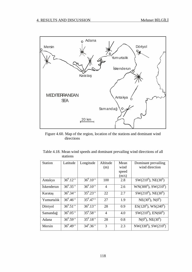
4. RESULTS AND DISCUSSION Mehmet BİLGİLİ
118
MEDITERRANEAN SEA
İskenderun
Antakya
Yumurtalık
Kara taş
Dörtyol
Adana
Mersin
Samandağ
20 km
Figure 4.60. Map of the region, location of the stations and dominant wind directions
Table 4.18. Mean wind speeds and dominant prevailing wind directions of all stations
Station Latitude Longitude Altitude(m)
Meanwindspeed(m/s)
Dominant prevailingwind direction
Antakya 360.12’’ 360.10’’ 100 2.8 SW(2100), NE(300)
İskenderun 360.35’’ 360.10’’ 4 2.6 WN(3000), SW(2100)
Karataş 360.34’’ 350.23’’ 22 2.7 SW(2100), NE(300)
Yumurtalık 360.46’’ 350.47’’ 27 1.9 NE(300), N(00)
Dörtyol 360.51’’ 360.13’’ 28 0.9 ES(1200), WS(2400)
Samandağ 360.05’’ 350.58’’ 4 4.0 SW(2100), EN(600)
Adana 360.59’’ 350.18’’ 28 0.8 N(00), NE(300)
Mersin 360.49’’ 340.36’’ 3 2.3 NW(3300), SW(2100)

4. RESULTS AND DISCUSSION Mehmet BİLGİLİ
119
Tabl
e 4.
19. C
orre
latio
n co
effic
ient
s of w
ind
spee
ds a
mon
gst s
tatio
ns
Dör
tyol
0.25
0.91
0.31
0.36
0.59
0.43
0.15 1
Ant
akya
0.18
0.14
0.41
0.67
0.29
0.76 1 0.15
Sam
andağ
0.06
0.44
0.69
0.85
0.59 1 0.76
0.43
Kar
ataş
0.24
0.66
0.74
0.72 1 0.59
0.29
0.59
İske
nder
un
0.02 0.4
0.76 1 0.72
0.85
0.67
0.36
Yum
urta
lık
0.1
0.46 1 0.76
0.74
0.69
0.41
0.31
Ada
na 0.04 1 0.46 0.4
0.66
0.44
0.14
0.91
Mer
sin 1 0.04 0.1
0.02
0.24
0.06
0.18
0.25
Stat
ion
Dör
tyol
Ant
akya
Sam
andağ
Kar
ataş
İske
nder
un
Yum
urta
lı
k Ada
na
Mer
sin

4. RESULTS AND DISCUSSION Mehmet BİLGİLİ
120
In this study, a model was developed to estimate wind speed of any target
station utilizing wind speeds of the reference measuring stations. Firstly, the mean
monthly wind speed obtained at 8 measuring stations in the eastern Mediterranean
region of Turkey were compared with each other and the correlation coefficients
between them two by two were determined. The accuracy of the results is basically
depended on the cross-correlation level between the two stations’ wind speed, which
is related to the morphology of the surrounding area (Bechrakis and Sparis, 2004).
Thus, the relation amongst stations was defined and reference stations were
determined for any target station. For the mean monthly wind speed between 1992
and 2001 the correlation coefficients of wind speeds amongst stations are presented
in Table 4.19. As seen in this table, Antakya, İskenderun, Karataş, Mersin, Samandağ
and Yumurtalık were defined as target stations sequentially except Adana and
Dörtyol stations due to a high rate of correlation factors.
4.5.2. Artificial Neural Network Architecture
Artificial neural network architecture used in this study for Karataş
meteorological station which is selected as a target station is shown in Figure 4.61.
This network consists of an input layer, two hidden layers and an output layer. The
mean monthly wind speeds of reference stations and corresponding month were used
in the input layer of the network. İskenderun, Yumurtalık, Adana and Samandağ
stations were selected as a reference stations. The most significant point in the
selection of these reference stations is that there is a good relation with high
correlation coefficient between the target station and reference station. The mean
monthly wind speed of Karataş which is target station was used in the output layer of
the network. For other target stations, the reference stations in the input layer of the
network, the number of the neurons in the hidden layers of the network and the
number of patterns in the training and testing procedure are given in Table 4.20.
Resilient propagation (RP) learning algorithm was used in the present simulation.
Neurons in the input layer have no transfer function. Logistic sigmoid transfer
function (logsig) and linear transfer function (purelin) were used in the hidden layers

4. RESULTS AND DISCUSSION Mehmet BİLGİLİ
121
and output layer of the network as an activation function, respectively. Simulations
were performed to estimate the mean monthly wind speed of target station. In each
layer, every neuron is connected to a neuron of adjacent layer having different
weights. Each neuron as indicated in Figure 4.61, receives signals from the neurons
of the previous layer weighted by the interconnect values between neurons except
input layer. Neurons then produce an output signal by passing the summed signal
through an activation function (Maqsood et al., 2005). Mohandes et al. (2004) stated
that during the training procedure, the weights of the connections between neurons
are adjusted in order to achieve the desired input/output relation of the network. This
procedure goes on until the difference between the actual output of the network and
the desired output is equal with a specified remainder value. Here, the criterion is put
forward as the network output which should be closer to the value of desired output.
This training procedure has to be repeated for the rest of the input-output pairs
existing in the training data.
Input layer
MonthWind speedof İskenderun
Wind speedof Yumurtalık
Wind speedof Karataş
Wind speedof Adana
Wind speedof Samandağ
Firsthidden layer
Secondhidden layer
Output layer
Figure 4.61. ANN architecture

4. RESULTS AND DISCUSSION Mehmet BİLGİLİ
122
Table 4.20. Reference stations and number of neurons in the hidden layers of the network for target stations
Targetstation
Reference stations Number ofneurons in
hiddenlayers
Number ofpatterns in
training
Number ofpatterns in
testing
Antakya İskenderun,Mersin
6-6 95 24
İskenderun Yumurtalık,Mersin, Antakya,Samandağ, Karataş
12-6 75 24
Karataş İskenderun,Yumurtalık,Adana, Samandağ
10-5 73 24
Mersin Antakya,İskenderun
6-3 95 24
Samandağ Karataş,İskenderun,Yumurtalık
8-4 75 24
Yumurtalık Adana, Samandağ,Karataş,İskenderun
10-5 73 24
4.5.3. Results and Discussion
In the present study, it is realized that artificial neural network is convenient
method to apply for the prediction of the wind speed. The mean absolute percentage
error (MAPE) was used to see the convergence between the target value and the
output value. In addition, the coefficient of correlation between the target value and
output value is defined as follows (Perez-Llera et al., 2002),
( ) ( )2 22 2
. .
.
t o t oRt t o o
-=
é ù é ù- -ê ú ê úë û ë û
(4.5.1)
Where, t is the target value, o is the output value, n is the total number of
months, t is the mean of the ti’s, o is the mean of oi’s and .t o is the mean of the
ti.oi’s.

4. RESULTS AND DISCUSSION Mehmet BİLGİLİ
123
ANNs have two step procedure; these are called training and testing
procedure. They are initially trained and then their accuracy is checked with the
testing database. ANN can give different results for each test using algorithm
constructed in the present work. Therefore, 10 tests were performed for each
meteorological station separately and for the most appropriate result, average values
of these tests were taken. The performance values for all stations, such as MAPE
and R for training and testing procedure are given in Table 4.21. The MAPE values
ranged from 4.49% to 14.13% differ from the actual value for all stations and testing
procedure. The maximum MAPE was found to be 14.13% for Antakya station in the
testing procedure, while the best result was found to be 4.49% for Mersin station in
the testing procedure. The maximum correlation coefficient between the target value
and output value was found to be 0.97 for testing procedure of Mersin station, while
the minimum correlation coefficient was found as 0.67 for Yumurtalık station.
Moreover, another significant point in this table, the performance values of the
training procedure are better than the performance values of the testing procedure.
Table 4.21. The performance values for training and testing procedure
Station Training procedure Testing procedure
MAPE R MAPE R
Antakya 5.53 0.97 14.13 0.96
İskenderun 1.48 0.99 9.97 0.87
Karataş 1.7 0.97 6.66 0.72
Mersin 3.44 0.96 4.49 0.97
Samandağ 3.07 0.95 8.83 0.83
Yumurtalık 2.56 0.97 13.25 0.67
In the present study, 2 years i.e. 24 months of hourly wind speed data from
the year 2000 to 2001 were taken for comparison. As seen in Figures 4.62-67,
prediction of ANN follows the variation of actual data exactly. In the case of
Antakya meteorological station, there are two sharp points with a level of 5 m/s
which correspond to the month of July, where as the lowest level of wind speed with

4. RESULTS AND DISCUSSION Mehmet BİLGİLİ
124
a level of 1.1 m/s which corresponds to the months of November and December as
indicated in Figure 4.62. Even though, the prediction of ANN agrees well with the
actual value. On the other hand, actual mean wind speed of İskenderun
meteorological station presented in Figure 4.63 varies rapidly from month to month,
though, the prediction of ANN for most of the months agrees well with the actual
values. It seems that as long as the necessary data are utilized for training and testing
procedure of the ANN method, it is possible to estimate an accurate result. It can be
concluded that the ANN looks promising in predicting the wind speed of a target
station depending on the selection of the reference measuring stations.
0
1
2
3
4
5
6
0 6 12 18 24
Month of the years (2000 and 2001)
Mea
n w
ind
spee
d (m
/s) actual
ANN
Figure 4.62. Comparison between prediction of ANN and actual results for Antakya meteorological station

4. RESULTS AND DISCUSSION Mehmet BİLGİLİ
125
0
1
2
3
4
5
0 6 12 18 24
Month of the years (2000 and 2001)
Mea
n w
ind
spee
d (m
/s) actual
ANN
Figure 4.63. Comparison between prediction of ANN and actual results for İskenderun meteorological station
0
1
2
3
4
0 6 12 18 24
Month of the years (2000 and 2001)
Mea
n w
ind
spee
d (m
/s)
actualANN
Figure 4.64. Comparison between prediction of ANN and actual results for Karataş meteorological station

4. RESULTS AND DISCUSSION Mehmet BİLGİLİ
126
0
1
2
3
4
0 6 12 18 24
Month of the years (2000 and 2001)
Mea
n w
ind
spee
d (m
/s)
actualANN
Figure 4.65. Comparison between prediction of ANN and actual results for Mersin meteorological station
0
1
2
3
4
5
6
0 6 12 18 24
Month of the years (2000 and 2001)
Mea
n w
ind
spee
d (m
/s)
actualANN
Figure 4.66. Comparison between prediction of ANN and actual results for Samandağ meteorological station

4. RESULTS AND DISCUSSION Mehmet BİLGİLİ
127
0
1
2
3
0 6 12 18 24
Month of the years (2000 and 2001)
Mea
n w
ind
spee
d (m
/s)
actualANN
Figure 4.67. Comparison between prediction of ANN and actual results for Yumurtalık meteorological station
4.6. Wind Speed Prediction Using Other Meteorological Variables
The amount of heat energy that is absorbed varies spatially as well as
temporally because of roughness of the earth surface. This creates ambient
temperature, atmospheric pressure and air density (specific mass) differences on the
earth. When the atmospheric air cools down, the density of the air increases and
hence the dense air collapse down due to the gravitational force. So, dense air causes
a high rate of pressure in close region of the earth surface. On the contrary, under
warm weather condition, atmospheric air expends, the rate of density decays down
and hence a low level of pressure region occurs along the earth surface. For this
reason, there is a pressure differences between cold and warm air regions. Air
movements attempt to balance the instability and finally, from a higher pressure
region to lower pressure region air movement occurs which is called wind speed
(Erol, 1999). The main parameters for the cause of air movement called wind are
atmospheric temperature, atmospheric pressure, air density and environmental
conditions. As a result, in order to predict wind speed one can use these
meteorological parameters.

4. RESULTS AND DISCUSSION Mehmet BİLGİLİ
128
Nowadays, renewable energy such as wind energy is one of the most
attractive sources of energy. Researches may need to prepare an inventory on the
availability of wind energy an area where the wind speed data are not available. For
this type of situation, it seems useful to predict the wind energy potential using ANN
method. Kalogirou et al. (1999) stated that the predicted variations of meteorological
parameters such as wind speed, relative humidity, solar radiation, air temperature,
etc. are needed in the industry of renewable energy for design purposes, performance
analysis and running cost of renewable energy systems. In addition, they reported
that for proper and efficient utilization of wind power, it is very important to know
the statistical characteristics, persistence, availability, diurnal variation and
prediction of wind speed. The values of wind power distributions are needed for site
selection, performance prediction and planning of wind turbines. Moreover,
prediction of wind speed is needed for any regional inventory wind energy studies in
advance. In this sense, the establishment of a model for wind speed correlation in a
region is of great importance in the management of wind energy resources for power
generation as well as in other research fields related to energy conservation
(Bechrakis et al., 2004).
The aim of this work is to apply Multiple Linear Regression and Artificial
Neural Network models for wind speed prediction with using various meteorological
variables of Antakya, Mersin and Samandağ meteorological stations, located in the
south-eastern region of Turkey.
4.6.1. Analysis of meteorological variables
In this study, monthly meteorological variables, collected by the Turkish
State Meteorological Service (TSMS) at 3 measuring stations which are located in
Antakya, Mersin and Samandağ districts were presently used. These meteorological
variables measured during the years of 1996-2005 include wind speed, dominant
wind direction, ambient temperature, atmospheric pressure, relative humidity and
rainfall. Stations are located between 360.05” and 360.49” north latitude in the eastern
Mediterranean region of Turkey. Heights of meteorological stations of Antakya,

4. RESULTS AND DISCUSSION Mehmet BİLGİLİ
129
Mersin and Samandağ above the sea level are 100 meter, 3 meter and 4 meter
respectively. Except Antakya; Mersin and Samandağ meteorological stations are
located on the coastal site of the eastern Mediterranean region. Mediterranean
climate is dominant in this region, usually hot and dry in summer season, lukewarm
and rainy in winter season. But, climate properties vary depending on the level of the
height above the see level. On the slope of a mountain looking at the sea, an increase
of terrestrial effects on climate is observed. However, the weather in this region does
not show intensed terrestrial climate due to the Mediterranean See effect (Bilgili et
al., 2007).
Figures 4.68-70 present average monthly variation of meteorological
parameters such as wind speed, ambient temperature, atmospheric pressure, relative
humidity and rainfall for Antakya, Mersin and Samandağ meteorological stations,
respectively. As seen in these figures, the atmospheric temperature and the wind
speed increase, on the other hand, the atmospheric pressure and rainfall decrease for
Antakya and Mersin meteorological stations. For Samandağ meteorological station,
there is no relationship at all between the wind speed and other meteorological
parameters. For Antakya meteorological station, as seen in Figure 4.68, mean
monthly wind speed varies drastically between 1.7 and 5.2 m/s with an average value
of 3.0 m/s. The maximum monthly wind speed occurs in summer season, while the
minimum monthly wind speed occurs in winter season. It is shown that atmospheric
temperature varied between 8.4 0C and 27.9 0C with an average value of 18.4 0C. It is
obvious that, the maximum monthly atmospheric temperature occurs in summer
season, while the minimum monthly atmospheric temperature occurs in winter
season, as expected. This situation indicates that there is a good relationship between
the monthly wind speed and monthly atmospheric temperature. Furthermore,
monthly wind speeds are negatively correlated with atmospheric pressure.

4. RESULTS AND DISCUSSION Mehmet BİLGİLİ
130
0
10
20
30
40
50
60
70
80
1 2 3 4 5 6 7 8 9 10 11 12
Month of the year
Atm
osph
eric
tem
pera
ture
(0 C
)R
elat
ive
hum
idity
(%)
Rai
nfal
l (cm
)
0
1
2
3
4
5
6
Atm
osph
eric
pre
ssur
e (b
ar)
Win
d sp
eed
(m/s
)
atmospheric temperature relative humidityrainfall wind speedatmosferic pressure
Figure 4.68. Average monthly variation of meteorological parameters for Antakya meteorological station
0
10
20
30
40
50
60
70
80
1 2 3 4 5 6 7 8 9 10 11 12
Month of the year
Atm
osph
eric
tem
pera
ture
(0 C
)R
elat
ive
hum
idity
(%)
Rai
nfal
l (cm
)
0
0,5
1
1,5
2
2,5
3
3,5
Atm
osph
eric
pre
ssur
e (b
ar)
Win
d sp
eed
(m/s
)
atmospheric temperature relative humidityrainfall wind speedatmosferic pressure
Figure 4.69. Average monthly variation of meteorological parameters for Mersin meteorological station

4. RESULTS AND DISCUSSION Mehmet BİLGİLİ
131
0
10
20
30
40
50
60
70
80
1 2 3 4 5 6 7 8 9 10 11 12
Month of the year
Atm
osph
eric
tem
pera
ture
(0 C)
Rel
ativ
e hu
mid
ity (%
)R
ainf
all (
cm)
0
1
2
3
4
5
6
Atm
osph
eric
pre
ssur
e (b
ar)
Win
d sp
eed
(m/s
)
atmospheric temperature relative humidityrainfall wind speedatmosferic pressure
Figure 4.70. Average monthly variation of meteorological parameters for Samandağ meteorological station
In order to obtain models of prediction for wind speed with various
meteorological variables using MLR and ANN methods, the first step in this analysis
is the selection of the independent variables. Here, the most significant point is the
fact that there is a high rate of correlation coefficient between the wind speed which
is the dependent variable and the various meteorological variables which are the
independent variables. Here, independent related variable must be only included to
the model. Because, the regression model must be established in a way that the best
estimation should be performed using a few independent variables as much as
possible (Sahinler, 2000). For this purpose, the diagrams of measured wind speeds
of each meteorological station are constructed against other meteorological data and
the correlation coefficients between all variables were calculated by taking them two
by two. The results obtained for Antakya, Mersin and Samandağ meteorological
stations are shown in Tables 4.22-24, respectively. An adequate value of the cross
correlation function for an accurate simulation must be higher than 0.6 (Bechrakis et
al., 2004). Therefore, as it is shown in these tables, significant correlation

4. RESULTS AND DISCUSSION Mehmet BİLGİLİ
132
coefficients were indicated in bold. This means that these parameters have a strong
correlation with each other. There is a high rate of correlation coefficient between the
wind speed and various meteorological variables such as atmospheric temperature
and pressure for Antakya and Mersin meteorological stations. Wind speeds are
positively correlated with atmospheric temperature in these meteorological stations,
while wind speeds are negatively correlated with atmospheric pressure. Because of
the fact that, in order to obtain prediction models for wind speed of Antakya and
Mersin meteorological stations, it can be selected atmospheric temperature and
pressure as independent (predictor) variables. In addition, for Samandağ
meteorological station, there is no high rate of correlation coefficient between the
wind speed and various meteorological variables. Because of inconsistency between
the wind speed and other meteorological variables, simulations of prediction models
may provide misleading results.
Table 4.22. Correlation coefficients between all meteorological variables for Antakya meteorological station
Windspeed
Winddirection
Atm.temperature
Atm.pressure
Relativehumidity
Rainfall
Wind speed 1 0.68 0.83 -0.91 -0.07 -0.52
Wind direction 1 0.81 -0.77 -0.17 -0.35
Atm. temperature 1 -0.90 -0.18 -0.55
Atm. pressure 1 0.09 0.41
Relative humidity 1 0.23
Rainfall 1

4. RESULTS AND DISCUSSION Mehmet BİLGİLİ
133
Table 4.23. Correlation coefficients between all meteorological variables for Mersin meteorological station
Windspeed
Winddirection
Atm.temperature
Atm.pressure
Relativehumidity
Rainfall
Wind speed 1 -0,44 0.74 -0.85 0.55 -0.40
Wind direction 1 -0.37 0.52 -0.53 -0.22
Atm. temperature 1 -0.88 0.52 -0.48
Atm. pressure 1 -0.69 0.39
Relative humidity 1 -0.01
Rainfall 1
Table 4.24. Correlation coefficients between all meteorological variables for Samandağ meteorological station
Windspeed
Winddirection
Atm.temperature
Atm.pressure
Relativehumidity
Rainfall
Wind speed 1 0.04 0.10 -0.30 0.34 -0.13
Wind direction 1 0.78 -0.74 0.65 -0.62
Atm. temperature 1 -0.88 0.59 -0.60
Atm. pressure 1 -70 0.55
Relative humidity 1 -0.27
Rainfall 1
4.6.2. Results for Multiple Regression Analysis
It is also well known that wind speed is related to various meteorological
variables in the atmosphere such as atmospheric temperature, atmospheric pressure,
air density and other air variables in the environment (Erol, 1999). As it is stated in
Tables 4.22 and 23, wind speeds are correlated wit atmospheric temperature and
pressure for Antakya and Mersin meteorological stations as expected. In the multiple
regression method, the most significant point is to select the predictor variables that
provide the best prediction equation for modeling of dependent variable. For
instance, atmospheric temperature and pressure were selected as the independent
variables in order to obtain predictive equation for modeling of wind speed. These
two independent variables were then used as a predictor variable in the multiple

4. RESULTS AND DISCUSSION Mehmet BİLGİLİ
134
regression analysis. By using the data between the years 1996 and 2001, the
following model was obtained for Antakya, Mersin and Samandağ meteorological
stations, respectively. Here, the dimensions of meteorological data such as wind
speed, atmospheric temperature and pressure are taken as m/s, 0C and mbar
respectively.
[ ] [ ] [ ]221.39 0.00910 . 0.21864 .wind speed atm temperature atm pressure= + -
[ ] [ ] [ ]93.164 0.00230 . 0.08977 .wind speed atm temperature atm pressure= - -
[ ] [ ] [ ]151.30 0.07911 . 0.14383 .wind speed atm temperature atm pressure= - -
The monthly wind speeds between the years 2002 and 2005 were predicted
using these equations for Antakya, Mersin and Samandağ meteorological stations,
separately. The scatter diagrams of the regression predictions against the actual
values were drawn for these meteorological stations in order to indicate the
performance of the MLR model. Especially for Antakya and Mersin meteorological
stations, as seen in Figures 4.71 and 72, the predicted results are as fairly close to the
corresponding actual measurements. In addition, as seen in Figure 4.73, because of
the low rate of correlation coefficient between the wind speed and other
meteorological variables for Samandağ meteorological station, the predicted results
are not in good agreement with the corresponding actual measurements as expected.

4. RESULTS AND DISCUSSION Mehmet BİLGİLİ
135
0
1
2
3
4
5
0 6 12 18 24 30 36 42 48
Month of the years (2002-2005)
Mea
n w
ind
spee
d (m
/s)
actualprediction (MLR)
Figure 4.71. Comparison between prediction of MLR and actual results for Antakya meteorological station
1
1,5
2
2,5
3
0 6 12 18 24 30 36 42 48Month of the years (2002-2005)
Mea
n w
ind
spee
d (m
/s)
actualprediction (MLR)
Figure 4.72. Comparison between prediction of MLR and actual results for Mersin meteorological station

4. RESULTS AND DISCUSSION Mehmet BİLGİLİ
136
2
3
4
5
6
0 6 12 18 24 30 36 42Month of the years (2002-2005)
Mea
n w
ind
spee
d (m
/s)
actualprediction (MLR)
Figure 4.73. Comparison between prediction of MLR and actual results for Samandağ meteorological station
4.6.3. Results for Artificial Neural Networks
Artificial neural network architecture used in this study is shown in Figure
4.74. This network consists of an input layer, a hidden layer and an output layer.
Monthly atmospheric temperature and pressure were used in the input layer of the
network. In addition, monthly wind speed was used in the output layer of the
network. Meteorological data measured during the period of 1996-2005 were divided
into two sections. The first section of the data which covers the years between 1996
and 2001 was used for training process. The second part of the data which covers the
years of 2002 and 2005 was utilized for testing process. Resilient propagation (RP),
Scaled Conjugate Gradient (SCG) and Levenberg-Marquardt (LM) learning
algorithm were applied in the present simulation. Neurons in the input layer have no
transfer function. Logistic sigmoid transfer function (logsig) was used in the hidden
layers and output layer of the network as an activation function. The values applied
in the input and output layers were normalized by the following formula in the range
of (0-1) (Krauss et al., 1997).

4. RESULTS AND DISCUSSION Mehmet BİLGİLİ
137
min
max min
( )( )
RN
X XXX X
-=
- (4.6.1)
Input layer
Atmospherictemperature
Wind speedAtmosphericpressure
Hidden layer Output layer
Figure 4.74. ANN architecture
Where, XN is normalized value, XR is real value, Xmin is minimal value and
Xmax is maximal value. Normalizing of the training inputs generally improves the
quality of the training (Krauss et al., 1997). Simulations were performed to estimate
the mean monthly wind speed using atmospheric temperature and pressure. As
Maqsood et al. (2005) reported that in each layer, every neuron is connected to a
neuron of adjacent layer having different weights. Each neuron as indicated in Figure
4.74, receives signals from the neurons of the previous layer weighted by the
interconnect values between neurons except input layer. Neurons then produce an
output signal by passing the summed signal through an activation function.
Mohandes et al. (2004) stated that during the training process, the weights of the
connections between neurons are adjusted in order to achieve the desired
input/output relation of the network. This procedure goes on until the difference
between the actual output of the network and the desired output is equal with a
specified remainder value. Here, the criterion is put forward as the network output
which should be closer to the value of desired output. This training process has to be

4. RESULTS AND DISCUSSION Mehmet BİLGİLİ
138
repeated for the rest of the input-output pairs existing in the training data. The scatter
diagrams of the network predictions against the actual values were drawn for all
meteorological stations in order to indicate the performance of the ANN method. As
seen in Figures 4.75-77, the results of prediction have fairly close agreement with the
corresponding actual measurements for all stations.
0
1
2
3
4
5
0 6 12 18 24 30 36 42 48
Month of the years (2002-2005)
Mea
n w
ind
spee
d (m
/s)
actualprediction (RP)
Figure 4.75. Comparison between prediction of RP and actual results for Antakya meteorological station
1
1,5
2
2,5
3
0 6 12 18 24 30 36 42 48
Month of the years (2002-2005)
Mea
n w
ind
spee
d (m
/s)
actualprediction (RP)
Figure 4.76. Comparison between prediction of RP and actual results for Mersin meteorological station

4. RESULTS AND DISCUSSION Mehmet BİLGİLİ
139
2
3
4
5
6
0 6 12 18 24 30 36 42
Month of the years (2002-2005)
Mea
n w
ind
spee
d (m
/s)
actualprediction (RP)
Figure 4.77. Comparison between prediction of RP and actual results for Samandağ meteorological station
4.6.4. Comparative Analysis of MLR model to ANN model
MLR and ANN models attempt to minimize sum squares of error between
experimentally measured and predicted values. Regression requires an explicit
function to be defined before the least squares parameter estimates, while a neural
network depends further more on the training data and the learning algorithm (Li et
al., 2001).
For comparative analysis of MLR model to ANN model, the mean absolute
percentage error (MAPE) and the correlation coefficient (R) were used to see the
convergence between the target values and the output values.
The performance values of MLR and ANNs methods (RP, SCG and LM
learning algorithm), such as MAPE and the correlation coefficient, R are given in
Table 4.25 for all stations. The MAPE values of MLR model differ from the actual
value of monthly wind speeds with the range of 8.57% and 17.05%. On the other
hand, the MAPE values of ANNs (RP) method ranged from 7.82% to 10.88% differ
from the actual value of monthly wind speed. However, the maximum MAPE was
found to be 17.05% for Antakya meteorological station in the MLR model, while

4. RESULTS AND DISCUSSION Mehmet BİLGİLİ
140
ANNs (RP) method provided that the best result was found to be 7.82% for Mersin
meteorological station, the maximum correlation coefficient between the target value
and output value was 0.96 for Antakya meteorological station. On the other hand,
MLR model provided that the minimum correlation coefficient was found as 0.38 for
Samandağ meteorological station which is expected, because of the low rate of
correlation coefficient between the wind speed and other meteorological variables.
As seen in this table, the performance values of the ANNs method are better than the
performance values of the MLR model. Moreover, another significant point in this
table, because of the high rate of correlation coefficient between the wind speed and
other meteorological variables, the performance values of Antakya and Mersin
meteorological stations are better than the performance values of Samandağ
meteorological station.
Table 4.25. Performance values of prediction results for all stations
Station
MLR method ANN method
RP algorithm SCG algorithm LM algorithm
MAPE R MAPE R MAPE R MAPE R
Antakya 17.05 0.92 10.88 0.96 11.00 0.96 11.70 0.95
Mersin 8.57 0.89 7.82 0.92 8.47 0.90 8.75 0.89
Samandağ 12.61 0.38 10.10 0.71 10.04 0.66 11.36 0.62
The aim of the present work is to try to predict wind speed using monthly
meteorological variables, and establish a model between these variables. For this
purposes, methods of multiple linear regression analysis and artificial neural network
were used. Results of these methods were compared to each other. In order to
improve the accuracy of predictions a few independent parameters or initial
parameters were used and related independent parameters were only included to the
model. Between monthly wind speed and meteorological variables such as
atmospheric temperature and pressure a good relations were obtained for Antakya
and Mersin meteorological stations, and hence using ANN and MLR methods
provide acceptable wind speeds for both stations. On the other hand, since there was

4. RESULTS AND DISCUSSION Mehmet BİLGİLİ
141
no a satisfactory relations between wind speed and independent variables such as
atmospheric temperature and pressure, these methods did not provide a predicted
results with an acceptable error in it for Samandağ meteorological station.
It was concluded that if there is good relations between wind speed and other
meteorological variables such as atmospheric temperature and pressure, wind speed
with these meteorological variables can be predicted with acceptable accuracy using
ANN and MLR methods.
4.7. Daily, Weekly and Monthly Wind Speed Predictions of Target StationUsing Artificial Neural Networks
4.7.1. Preparation of Input and Output Data
In this study, the ANN method was applied for the prediction of the daily,
weekly and monthly wind speed of any target station at a location with no
measurement, which is referred to as the target station from the measurements of a
set of surrounding stations. This study has been applied for regional wind speed
prediction in some parts of the Aegean and Marmara region of Turkey. This wind
speed prediction of any pivot station was based on the wind speeds of neighboring
measuring stations. In order to estimate a target station, the correlation coefficient
was obtained for each pair of wind speed time series of all stations and weighting
factors between the pivot station and its surrounding stations were determined by
artificial neural network technique.
The data used in this study were collected from Gökçeada, Foca, Gelibolu
and Bababurnu stations which have been set up by the General Directorate of
Electrical Power Resources Survey Administration (EIE). The map of the region and
the location of the stations are presented in Figure 4.78. Geographical coordinates
and measurement periods of these stations are given in Table 4.26. Stations extend
from latitude 38039’25” to 40026’34” north and longitude 25057’00” to 26046’22”
east, while the heights of stations above the sea level vary between 175 meter and
348 meter. These stations located in the Marmara and Aegean region of Turkey
supply wind speed and direction every one hour. The Marmara region comes under

4. RESULTS AND DISCUSSION Mehmet BİLGİLİ
142
the influence of the mild Mediterranean climate during the summer months. During
the winter time, this region is under the influence of high pressure of Siberia and the
Balkan Peninsula and, consequently, northeasterly or westerly winds influence the
area with high rainfall amounts in addition to snow every year with cold and wet
spells (Öztopal, 2006). In the Aegean region geomorphological features have long
valleys that run perpendicular to the coast. These are parallel to the cyclonic
movements that originate from the Genoa bay and move towards the east and
therefore show strong wind effects at the Aegean coast as well as the moving air
which penetrates deep in these valleys (Durak and Şen, 2002).
36
28 32
FocaAegean Sea
Marmara Sea
Black Sea
GökçeadaBababurnu
TURKEY
Gelibolu
Figure 4.78. The map of the region and the location of the stations
Table 4.26. Geographical coordinates and measurement periods of stations
Station Latitude Longitude Altitude(m)
Period Anemometerheight (m)
Gökçeada 400 07’ 58” N 250 57’ 00” E 244 1998-2003 10
Foca 380 39’ 25” N 260 46’ 22” E 175 1998-2003 10
Gelibolu 400 26’ 34” N 260 32’ 56” E 302 1998-2003 10
Bababurnu 390 30’ 03” N 260 12’ 39” E 348 1998-2003 10

4. RESULTS AND DISCUSSION Mehmet BİLGİLİ
143
The sensors measuring wind speed and direction of all stations are situated 10
m above the ground level. The long-term wind data cover the period from the year
1998 to 2003. The daily, weekly, monthly and annual wind data were obtained using
the averages of hourly wind data. The annual average wind speed, energy potential
and dominant prevailing wind direction of all stations for the year 2001 are presented
in Table 4.27. It is seen from the table that the annual average wind speeds range
from a low of 5.7 m/s in Foca station to a high of 7.2 m/s in Gökçeada station. The
standard deviation of wind speeds varies mainly from a low level of 2.6826 to a
maximum level of 4.3673. These regions are highly suitable for wind power
generation. While the highest annual wind energy potential value is determined as
518 W/m2 in Gökçeada station, the lowest annual wind energy potential value is
found as 196 W/m2 in Foca station. The annual wind energy potential values of
Bababurnu and Gelibolu stations are determined as 254 W/m2 and 406 W/m2,
respectively. As it is mentioned in Table 4.27, the dominant prevailing wind
directions for Gökçeada, Foca, Gelibolu and Bababurnu stations are 2100, 300, 900
and 300, on the other hand the effect of wind that is observed at the lowest degree is
in the direction of 900, 2400, 1500 and 2700, respectively. The direction of the wind is
of decisive significance for the evaluation of the possibilities of utilizing wind power.
Scatter diagrams of the monthly average wind speeds of stations for the year 2001
are presented in Figure 4.79. It is interesting to note that the monthly average wind
speeds of stations show the same variation according to each other. It is also clear
from the figure that the four curves have similar changing trends, but the rate of
change is not the same. A dramatic variation in the monthly average wind speed
occurs during a year at these stations. The maximum monthly average wind speed
occurs in December; on the other hand the minimum monthly average wind speed
occurs in April and September for all stations. The monthly average wind speeds
range from a low of 4.6 m/s in Bababurnu station to a high of 10.8 m/s in Gökçeada
station. The minimum and maximum monthly average wind speeds of Gökçeada
station which has the highest value among these stations are 5.3 m/s and 10.8 m/s,
respectively.

4. RESULTS AND DISCUSSION Mehmet BİLGİLİ
144
Table 4.27. The annual average wind speed, energy potential and dominant wind direction of stations in 2001
StationMean wind
speed(m/s)
Standarddeviation
Mean windenergy potential
(W/m2)
Dominantwind
directionGökçeada 7.2 4.3673 518 SW (2100)
Foca 5.7 2.6826 196 NE (300)
Gelibolu 6.8 3.8692 406 E (900)
Bababurnu 6.0 3.1618 254 NE (300)
1 2 3 4 5 6 7 8 9 10 11 12Foca
BababurnuGelibolu
Gökçeada
0
2
4
6
8
10
12
Windspeed (m/s)
Month (2001)
Figure 4.79. Monthly average wind speed of stations
4.7.2. Application
Artificial neural network architecture used in this study is shown in Figure
4.80. It can be seen from the figure that three station wind speeds (Foca, Gelibolu
and Bababurnu) were used as input neurons in the ANN architecture, while target
station wind speed (Gökçeada) was used as output neuron in the ANN architecture.
Similar to this architecture, input and output neurons in the ANN architecture can be
changed according to the selection of the target station. This network consists of an

4. RESULTS AND DISCUSSION Mehmet BİLGİLİ
145
input layer, a hidden layer and an output layer. Resilient propagation (RP), scaled
conjugate gradient (SCG) and Levenberg-Marquardt (LM) learning algorithms were
applied in the present simulation. Neurons in the input layer have no transfer
function. Logistic sigmoid transfer function (logsig) and linear transfer function were
used in the hidden layers and output layer of the network as an activation function,
respectively. Simulations were performed to predict the daily, weekly and monthly
average wind speed of target station using reference stations data.
Input layer
Wind speed of Foca
Wind speed of Gökçeada
Wind speed of Gelibolu
Wind speed of Bababurnu
Hidden layer Output layer
Figure 4.80. Artificial Neural Network architecture
4.7.2.1. Daily Prediction
Here, a model was developed to predict the daily wind speed of any pivot
station utilizing wind speeds of the reference measuring stations. The wind speed
data used in this study was measured between January 1 and December 31 for the
year 2001. Firstly, the daily average wind speed data was obtained using the averages
of hourly wind data. Then, in order to designate relationship amongst stations, the
daily average wind speeds of all stations were compared with each other and the
correlation coefficients between them two by two were determined. The accuracy of
the results is basically depended on the cross-correlation level between the two
stations’ wind speed, which is related to the morphology of the surrounding area
(Bechrakis et al., 2004). The correlation coefficients of daily wind speeds amongst

4. RESULTS AND DISCUSSION Mehmet BİLGİLİ
146
stations are presented in Table 4.28. It is also clear from the table that there is a high
rate of correlation coefficient between the daily wind speeds. These correlation
coefficients range from a low level of 0.65445 between Gelibolu and Foca stations to
a high level of 0.91782 between Gelibolu and Gökçeada stations.
Table 4.28. Correlation coefficients of daily wind speeds between stations
Station Gökçeada Foca Gelibolu Bababurnu
Gökçeada 1 0.72372 0.91782 0.78539
Foca 0.72372 1 0.65445 0.82579
Gelibolu 0.91782 0.65445 1 0.7092
Bababurnu 0.78539 0.82579 0.7092 1
The total available daily average wind speed data for each station (365 days)
was divided into two parts. The first part of the data (334 days) was used for training
process, while the second part of the data which covers the days between October 1
and October 31 (31 days) was used for testing process. Training data is used to
design the model, while the testing data is used to predict the performance of the
network. Three station wind speeds were used as input neurons in the ANN
architecture, while target station wind speed was used as an output neuron in the
ANN architecture. The scatter diagrams of the network predictions against the actual
values were drawn for all stations in order to indicate the performance of the ANN
method. It can be seen from Figures 4.81-84 that the results of prediction have fairly
close agreement with the corresponding measurements for all stations. The daily
average wind speed varies rapidly from day to day, though the prediction of ANN for
most of the days agrees well with the actual values.

4. RESULTS AND DISCUSSION Mehmet BİLGİLİ
147
0
4
8
12
16
20
0 5 10 15 20 25 30Day (October 2001)
Win
d sp
eed
(m/s
)Actual ANN (RP_6)ANN (LM_6) ANN (SCG_6)
Figure 4.81. Comparison between predictions of ANN and daily measured wind speeds for Gökçeada station
0
4
8
12
0 5 10 15 20 25 30Day (October 2001)
Win
d sp
eed
(m/s
)
Actual ANN (RP_6)ANN (LM_6) ANN (SCG_6)
Figure 4.82. Comparison between predictions of ANN and daily measured wind speeds for Foca station

4. RESULTS AND DISCUSSION Mehmet BİLGİLİ
148
0
4
8
12
16
0 5 10 15 20 25 30Day (October 2001)
Win
d sp
eed
(m/s
)Actual ANN (RP_6)ANN (LM_6) ANN (SCG_6)
Figure 4.83. Comparison between predictions of ANN and daily measured wind speeds for Gelibolu station
0
4
8
12
16
0 5 10 15 20 25 30Day (October 2001)
Win
d sp
eed
(m/s
)
Actual ANN (RP_6)ANN (LM_6) ANN (SCG_6)
Figure 4.84. Comparison between predictions of ANN and daily measured wind speeds for Bababurnu station

4. RESULTS AND DISCUSSION Mehmet BİLGİLİ
149
4.7.2.2. Weekly Prediction
The wind speed data used in this study was measured between January 1 and
December 31 for the year 2001. The weekly average wind speed data was obtained
using the averages of hourly wind data. The correlation coefficients of weekly wind
speeds amongst stations are presented in Table 4.29. It is also clear from the table
that there is a high rate of correlation coefficient between the weekly wind speeds.
These correlation coefficients range from a low level of 0.65191 between Gelibolu
and Foca stations to a high level of 0.92717 between Gelibolu and Gökçeada
stations.
Table 4.29. Correlation coefficients of weekly wind speeds between stations
Station Gökçeada Foca Gelibolu Bababurnu
Gökçeada 1 0.7792 0.92717 0.82427
Foca 0.7792 1 0.65191 0.9006
Gelibolu 0.92717 0.65191 1 0.73252
Bababurnu 0.82427 0.9006 0.73252 1
The total available weekly average wind speed data for each station (52
weeks) was divided into two parts. The first part of the data (40 weeks) was used for
training process, while the second part of the data which covers the weeks between
July 16 and October 7 (12 weeks) was used for testing process. The scatter diagrams
of the network predictions against the actual values were drawn for all stations in
order to indicate the performance of the ANN method. Figures 4.85-88 reveal that
predictions of ANN follow the variation of experimentally measured data exactly.

4. RESULTS AND DISCUSSION Mehmet BİLGİLİ
150
0
2
4
6
8
10
12
0 2 4 6 8 10 12Week (July 16, 2001 -October 7, 2001)
Win
d sp
eed
(m/s
)
Actual ANN (RP_6)ANN (LM_6) ANN (SCG_6)
Figure 4.85. Comparison between predictions of ANN and weekly measured wind speeds for Gökçeada station
0
2
4
6
8
10
0 2 4 6 8 10 12Week (July 16, 2001 -October 7, 2001)
Win
d sp
eed
(m/s
)
Actual ANN (RP_6)ANN (LM_6) ANN (SCG_6)
Figure 4.86. Comparison between predictions of ANN and weekly measured wind speeds for Foca station

4. RESULTS AND DISCUSSION Mehmet BİLGİLİ
151
0
2
4
6
8
10
12
0 2 4 6 8 10 12
Week (July 16, 2001 -October 7, 2001)
Win
d sp
eed
(m/s
)
Actual ANN (RP_6)ANN (LM_6) ANN (SCG_6)
Figure 4.87. Comparison between predictions of ANN and weekly measured wind speeds for Gelibolu station
0
2
4
6
8
10
12
0 2 4 6 8 10 12
Week (July 16, 2001 -October 7, 2001)
Win
d sp
eed
(m/s
)
Actual ANN (RP_6)ANN (LM_6) ANN (SCG_6)
Figure 4.88. Comparison between predictions of ANN and weekly measured wind speeds for Bababurnu station

4. RESULTS AND DISCUSSION Mehmet BİLGİLİ
152
4.7.2.3. Monthly Prediction
The wind speed data used in this study was experimentally measured between
the years 1998 and 2003. The correlation coefficients of monthly wind speeds
amongst stations are presented in Table 4.30. These correlation coefficients range
from a low level of 0.64429 between Gökçeada and Foca stations to a high level of
0.87082 between Bababurnu and Foca stations. There are missing data for some
months due to faulty operation of the anemometer.
Table 4.30. Correlation coefficients of monthly wind speeds between stations
Station Gökçeada Foca Gelibolu Bababurnu
Gökçeada 1 0.64429 0.79538 0.64774
Foca 0.64429 1 0.81797 0.87082
Gelibolu 0.79538 0.81797 1 0.73022
Bababurnu 0.64774 0.87082 0.73022 1
The total available monthly average wind speed data for each station (47
months) was divided into two parts. The first part of the data (35 months) was used
for training process, while the second part of the data which covers the months in the
year of 2001 (12 months) was used for testing process. The scatter diagrams of the
network predictions against the experimentally measured values were presented for
all stations in order to indicate the performance of the ANN method. As seen in
Figures 4.89-92 that the results of prediction have fairly close agreement with the
corresponding experimentally measured wind speed data for all stations.

4. RESULTS AND DISCUSSION Mehmet BİLGİLİ
153
0
2
4
6
8
10
12
14
0 2 4 6 8 10 12Month (2001)
Win
d sp
eed
(m/s
)
Actual ANN (RP_6)ANN (LM_6) ANN (SCG_6)
Figure 4.89. Comparison between predictions of ANN and monthly measured wind speeds for Gökçeada station
0
2
4
6
8
0 2 4 6 8 10 12Month (2001)
Win
d sp
eed
(m/s
)
Actual ANN (RP_6)ANN (LM_6) ANN (SCG_6)
Figure 4.90. Comparison between predictions of ANN and monthly measured wind speeds for Foca station

4. RESULTS AND DISCUSSION Mehmet BİLGİLİ
154
0
2
4
6
8
10
0 2 4 6 8 10 12Month (2001)
Win
d sp
eed
(m/s
)
Actual ANN (RP_6)ANN (LM_6) ANN (SCG_6)
Figure 4.91. Comparison between predictions of ANN and monthly measured wind speeds for Gelibolu station
0
2
4
6
8
10
0 2 4 6 8 10 12Month (2001)
Win
d sp
eed
(m/s
)
Actual ANN (RP_6)ANN (LM_6) ANN (SCG_6)
Figure 4.92. Comparison between predictions of ANN and monthly measured wind speeds for Bababurnu station

4. RESULTS AND DISCUSSION Mehmet BİLGİLİ
155
4.7.3. Results and Discussion
In the present study, it is realized that artificial neural network is convenient
method to apply for the prediction of the wind speed. The mean absolute percentage
error (MAPE) and correlation coefficient (R) were used to see the convergence
between the target value and the output value. Firstly, training process is applied to
design the model. Then, testing process is applied to evaluate the performance of the
network. The performance values such as MAPE and R for learning and testing
process are given in Table 4.31. In the result of testing process, it can be seen from
the table that, the MAPE values ranged from 11.6909% to 16.7572% differ from the
actual value for daily wind speeds, while the MAPE values ranged from 4.7970% to
8.6794% and from 3.2376% to 7.5701% differ from the actual value for weekly and
monthly wind speeds, respectively. The maximum MAPE was found to be 16.7572%
for daily wind speeds in Gökçeada station. On the other hand, the best result was
found to be 3.2376% for monthly wind speeds in Gelibolu station. It is seen from the
table that the performance values of monthly wind speed prediction are better than
the performance values of weekly and daily wind speed prediction. Another
significant point in this table, the performance values of the learning process are in
general better than the performance values of the testing process. The maximum
correlation coefficient between the experimentally measured and predicted value was
found to be 0.9769 for monthly wind speeds of Gelibolu station in the SCG learning
algorithm. On the other hand, the minimum correlation coefficient was found as
0.8856 for monthly wind speeds of Foca station in the LM learning algorithm.

4. RESULTS AND DISCUSSION Mehmet BİLGİLİ
156
Tabl
e 4.
31. T
he p
erfo
rman
ce v
alue
s for
lear
ning
and
test
ing
proc
ess
a) F
or d
aily
win
d sp
eeds
Test
ing
proc
ess
SCG
_6
R 0.94
6
0.93
3
0.93
2
0.95
1
MA
PE
16.7
57
11.8
42
13.8
70
15.7
41
LM_6
R 0.94
1
0.93
7
0.94
5
0.95
1
MA
PE
16.5
93
12.2
79
13.9
86
16.6
93
RP_
6
R 0.95
2
0.94
1
0.93
4
0.94
9
MA
PE
15.1
30
11.6
91
13.4
01
16.6
28
Lear
ning
pro
cess
SCG
_6
R 0.95
0
0.86
1
0.92
3
0.90
2
MA
PE
15.3
40
13.7
88
16.6
82
15.0
57
LM_6
R 0.94
4
0.85
7
0.92
8
0.90
1
MA
PE
15.2
49
13.9
76
15.7
08
14.9
66
RP_
6
R 0.94
6
0.87
1
0.92
5
0.88
5
MA
PE
15.5
14
13.3
62
16.6
95
15.9
42
Stat
ion
Gök
çead
a
Foca
Gel
ibol
u
Bab
abur
nu

4. RESULTS AND DISCUSSION Mehmet BİLGİLİ
157
Tabl
e 4.
31. (
Con
tinue
d) T
he p
erfo
rman
ce v
alue
s for
lear
ning
and
test
ing
proc
ess
b) F
or w
eekl
y w
ind
spee
ds
Test
ing
proc
ess
SCG
_6
R 0.95
2
0.95
1
0.95
1
0.95
0
MA
PE 6.87
5
5.36
0
7.42
0
7.88
4
LM_6
R 0.95
7
0.94
8
0.95
0
0.95
3
MA
PE 6.84
7
4.79
7
7.22
2
8.44
7
RP_
6
R 0.97
3
0.94
9
0.97
2
0.94
8
MA
PE 5.88
5
5.31
9
5.76
0
8.67
9
Lear
ning
pro
cess
SCG
_6
R 0.97
1
0.95
2
0.94
4
0.98
7
MA
PE 5.65
8
4.70
0
7.25
4
2.94
5
LM_6
R 0.97
5
0.92
5
0.94
3
0.97
3
MA
PE 5.55
1
5.71
5
7.34
6
4.17
5
RP_
6
R 0.97
5
0.92
4
0.95
9
0.95
4
MA
PE 5.23
4
5.20
4
6.05
5
5.58
1
Stat
ion
Gök
çead
a
Foca
Gel
ibol
u
Bab
abur
nu

4. RESULTS AND DISCUSSION Mehmet BİLGİLİ
158
Tabl
e 4.
31. (
Con
tinue
d) T
he p
erfo
rman
ce v
alue
s for
lear
ning
and
test
ing
proc
ess
c) F
or m
onth
ly w
ind
spee
ds
Test
ing
proc
ess
SCG
_6
R 0.90
6
0.93
4
0.97
7
0.95
6
MA
PE 6.44
1
5.07
5
3.23
8
3.90
6
LM_6
R 0.96
1
0.88
6
0.93
1
0.94
7
MA
PE 7.57
0
5.37
0
5.61
2
4.43
3
RP_
6
R 0.97
2
0.92
9
0.95
8
0.94
7
MA
PE 4.71
2
4.68
4
3.89
3
4.83
6
Lear
ning
pro
cess
SCG
_6
R 0.88
8
0.96
4
0.96
6
0.95
4
MA
PE 7.68
6
2.77
6
3.72
2
3.32
2
LM_6
R 0.86
9
0.95
8
0.96
8
0.97
9
MA
PE 8.80
0
2.55
6
3.39
6
1.80
7
RP_
6
R 0.83
7
0.96
6
0.94
2
0.93
6
MA
PE 8.66
2
2.55
3
5.36
1
3.77
4
Stat
ion
Gök
çead
a
Foca
Gel
ibol
u
Bab
abur
nu

4. RESULTS AND DISCUSSION Mehmet BİLGİLİ
159
4.8. Prediction of Long Term Monthly Temperature and Rainfall in TurkeyUsing Artificial Neural Networks
4.8.1. Data Analysis and Climate of Turkey
The climate is one of the most important parameters for energy efficiency of
buildings. It is not possible to design an energy efficient building without having the
temperature, the solar radiation, the wind velocity data, etc. Bulut et al. (2003)
reported that the design of heating, ventilating and air-conditioning (HVAC) and
solar energy systems, the energy analysis of buildings and the calculation of cooling
and heating loads depend on the weather data.
One of the most important meteorological parameters is the air temperature.
That is the reason the air temperature is recorded regularly in a meteorological
stations worldwide. Guan et al. (2007) stated that it is also widely known that there is
a relationship between air temperature and other meteorological parameters such as
solar radiation, air humidity, atmospheric pressure and wind speed. Because of the
source of heat energy supplied to the Earth’s surface and the atmosphere comes
predominantly from the Sun, the variation in solar radiations has a major impact on
the weather conditions on the Earth which leads the air temperature to fluctuate. This
air temperature variations cause variations in the level of water evaporation and air
saturation, leading the air humidity to change. Furthermore, the air temperature
differences between different zones also cause an air pressure difference, which in
turn produces air movement.
Nowadays it is possible to predict the weather forecasting in terms of the
application of science and technology for a future time and a given location or any
region on the Earth. Guan et al. (2007) and, Maqsood and Abraham (2007) stated
that the weather forecasting is essential for the resource of many subjects, such as the
performance of buildings, agricultural production and critical information about
future weather. Estimating the properties of the weather helps to safeguard life and
properties, and play a crucial role in planning the activities of government, industry
and the public. Maqsood and Abraham (2007) reported that the weather phenomena
of a complex nature have a direct impact on the safety and/or economic stability.

4. RESULTS AND DISCUSSION Mehmet BİLGİLİ
160
Accurate weather forecast models are important to the regions, where the entire
agricultural depends upon weather, in particular at the present time. In addition,
Kalogirou et al. (1999) stated that the predicted variations of meteorological
parameters such as wind speed, relative humidity, solar radiation, air temperature,
rainfall etc. are needed in the industry of renewable energy for design purposes,
performance analysis and running cost estimation of renewable energy systems.
The experimental data used in this study were measured by the Turkish State
Meteorological Service (TSMS) at 76 measuring stations of Turkey. The long-term
monthly temperature and rainfall cover the period from the year 1975 to 2006.
Locations of the measuring stations are presented in Figure 4.93. As seen in this
figure, meteorological stations cover almost all parts of the country. Sixty-nine
stations are selected for training data, while seventeen stations in the different
regions of Turkey are used for testing data. Geographical coordinates of these
stations are indicated in Tables 4.32 and 33. Stations extend from latitude 36.120 to
42.020 north and longitude 26.240 to 44.030 east, while the heights of stations above
the sea level vary between 3.4 meter and 1869 meter. These stations supply
meteorological variables such as temperatures and rainfalls in seven different regions
of Turkey. Scattering diagram of the long term monthly temperatures and rainfalls in
Turkey is presented in Figure 4.94. These data were obtained using average values of
temperatures and rainfalls taken from 76 measuring stations. It is also clear from
Figure 4.94 that the two curves present different changing trends according to each
other. A dramatic variation in the long term monthly temperature and rainfall in
Turkey occurs during a year. The long term monthly temperature ranges from a low
level of 2.09 0C in January to a high level of 24.39 0C in July. Where as, the long
term monthly rainfall ranges from a low level of 3.77 day in August to a high level of
12.46 day in December.
Turkey is situated in a large Mediterranean geographical region where
climatic conditions have a quite high temperate, diverse nature of the landscape, and
the existence of the mountains that run parallel to the Mediterranean and Black Sea
costs and perpendicular to the Aegean Sea cost which result in significant differences

4. RESULTS AND DISCUSSION Mehmet BİLGİLİ
161
in climatic conditions from one region to the other. In conclusion, Turkey's diverse
regions have different climates because of irregular topography (TSMS, 2007).
Black Sea
Marmara Sea
Aeg
ean
Sea
Mediterranean Sea32
28
28
32
36
36
363640
40
4040
44
44
TURKEYBurdur
Tekirdağ
Aydın
KütahyaBalıkesir
Sakarya KarsTrabzon
Erzincan
AmasyaKırıkkale
Mardin
Bingöl
Adıyaman
Nevşehir
AdanaKaraman
Figure 4.93. Locations of the measuring stations (○: stations used in training, ●: stations used in testing)
0
5
10
15
20
Jan. Feb. Mar. Apr. May Jun. Jul. Aug. Sep. Oct. Nov. Dec.
Month
Rai
nfal
l (da
y)
0
5
10
15
20
25
30
Tem
pera
ture
(0 C)
RainfallTemperature
Figure 4.94. Long term monthly temperature and rainfall of Turkey

4. RESULTS AND DISCUSSION Mehmet BİLGİLİ
162
Table 4.32. Geographical coordinates of the stations selected for training data
Station Latitude (0) Longitude (0) Altitude (m)
Ağrı 39.43 43.03 1632
Aksaray 38.23 34.03 960.77
Ankara 39.57 32.53 890.52
Antalya 36.52 30.42 47.328
Ardahan 41.07 42.43 1829
Artvin 41.11 41.49 628.35
Bartın 41.38 32.20 32.52
Batman 37.35 41.07 610
Bilecik 40.09 29.59 539.19
Bitlis 38.22 42.06 1573
Bolu 40.44 31.56 742.92
Bursa 40.13 29.00 100.32
Çanakkale 40.08 26.24 5.5
Çankırı 40.37 33.37 751
Çorum 40.33 34.58 775.91
Denizli 37.47 29.05 425.29
Diyarbakır 37.54 40.14 649
Düzce 40.50 31.10 145.67
Edirne 41.41 26.33 51.19
Elazığ 38.39 39.15 989.75
Erzurum 39.54 41.17 1869
Eskişehir 39.46 30.33 801
Gaziantep 37.03 37.21 854
Gümüşhane 40.28 39.28 1219
Hakkari 37.34 43.44 1727.74
Hatay 36.12 36.10 100
Iğdır 39.55 44.03’ 858
Isparta 37.45 30.33’ 996.88

4. RESULTS AND DISCUSSION Mehmet BİLGİLİ
163
Table 4.32. (Continued) Geographical coordinates of the stations selected for training data
Station Latitude (0) Longitude (0) Altitude (m)
İstanbul 40.58 29.05’ 32.98
İzmir 38.23 27.04’ 28.55
Kahramanmaraş 37.36 36.56 572.13
Kastamonu 41.22 33.47 799.91
Kayseri 38.43 35.29 1092
Kırklareli 41.44 27.13 231.5
Kırşehir 39.09 34.10 1007.17
Kilis 36.42 37.06 650
Kocaeli 40.46 29.56 76
Konya 37.52 32.28 1028.59
Malatya 38.21 38.13 947.87
Manisa 38.37 27.26 71
Mersin 36.48 34.38 3.4
Muğla 37.13 28.22 646.07
Muş 38.41 41.29 1322.76
Niğde 37.58 34.41 1210.5
Ordu 40.59 37.54 4.13
Osmaniye 37.06 36.15 99
Rize 41.02 40.30 8.6
Samsun 41.21 36.15 4
Siirt 37.55 41.57 895.54
Sinop 42.02 35.10 32
Sivas 39.45 37.01 1285
Şanlıurfa 37.09 38.47 547.187
Tokat 40.18 36.34 607.6
Tunceli 39.07 39.33 980.914
Uşak 38.41 29.24 919.22

4. RESULTS AND DISCUSSION Mehmet BİLGİLİ
164
Table 4.32. (Continued) Geographical coordinates of the stations selected for training data
Station Latitude (0) Longitude (0) Altitude (m)
Van 38.28 43.41 1670.52
Yalova 40.40 29.17 3.81
Yozgat 39.49 34.48 1298.43
Zonguldak 41.27 31.48 135.35
Table 4.33. Geographical coordinates of the stations selected for testing data
Station Latitude (0) Longitude (0) Altitude (m)
Adana 37.03 35.21 27
Adıyaman 37.45 38.17 672
Amasya 40.39 35.51 411.69
Aydın 37.51 27.51 56.3
Balıkesir 39.39 27.52 153
Bingöl 38.52 40.30 1177
Burdur 37.43 30.18 957
Erzincan 39.45 39.30 1218.22
Karaman 37.12 33.13 1023.05
Kars 40.37 43.06 1775
Kırıkkale 39.51 33.31 750.889
Kütahya 39.25 29.58 969.28
Mardin 37.18 40.44 1050
Nevşehir 38.37 34.42 1259.54
Sakarya 40.46 30.24 30.43
Tekirdağ 40.59 27.30 3.6
Trabzon 40.59 39.45 30

4. RESULTS AND DISCUSSION Mehmet BİLGİLİ
165
The Marmara region of Turkey comes under the influence of the mild
Mediterranean climate during the summer months. During the winter time, this
region is under the influence of high pressure of Siberia and the Balkan Peninsula
and, consequently, northeasterly or westerly winds influence the area with high
rainfall amounts in addition to snow every year with cold and wet spells (Öztopal,
2006).
In the Aegean region of Turkey geomorphologic features have long valleys
that run perpendicular to the coast. These are parallel to the cyclonic movements that
originate from the Genoa bay and move towards the east and therefore show strong
wind effects at the Aegean coast as well as the moving air which penetrates deep in
these valleys (Durak and Şen, 2002). The Aegean and Mediterranean coasts have
cool, rainy winters and hot, moderately dry summers.
In Eastern Anatolia and South-Eastern Anatolia there is a long winter, and
snow remains on the ground from November until the end of April. The climate in
the Black Sea area is wet, and humid. The Black Sea coast receives the greatest
amount of rainfall. The eastern part of that receives 2,200 millimeters annually and is
the only region of Turkey that receives rainfall throughout the year (TSMS, 2007).
4.8.2. Artificial Neural Network Architecture
In order to get the results in the best overall performance, several network
architectures were investigated. At the end of this analysis, the network architecture
used in this study was generated eventually. As seen in Figure 4.95, this network
architecture has one hidden layer with 32 neurons. Four neurons which receive input
signals of latitude, longitude, altitude and month were used in the input layer of the
network. Two neurons which produce corresponding output signals of the long term
monthly temperature and rainfall were utilized in the output layer of the network. In
order to train the neural network, meteorological and geographical data taken from
76 measuring stations were used as a training (59 stations) and testing (17 stations)
data. A total of 912 data sets (76 stations x 12 months) were divided into two parts.
From this set 708 data sets (59 stations x 12 months) were used for training
procedure of the network, while the remaining 204 data sets (17 stations x 12

4. RESULTS AND DISCUSSION Mehmet BİLGİLİ
166
months) were selected to be used as the testing procedure of the network. The
stations used for training and testing procedure are presented in Figure 4.93. The
stations used for the testing procedure are Adana, Adıyaman, Amasya, Aydın,
Balıkesir, Bingöl, Burdur, Erzincan, Karaman, Kars, Kırıkkale, Kütahya, Mardin,
Nevşehir, Sakarya, Tekirdağ and Trabzon. Training data is used to design the model,
while the testing data is used to predict the performance of the network. Levenberg-
Marquardt (LM-32) learning algorithm was applied in the present simulation.
Logistic sigmoid transfer function (logsig) and linear transfer function (purelin) were
used in the hidden layers and output layer of the network as an activation function,
respectively. Simulations were performed to predict the long term monthly
temperature and rainfall at any specific point of region of Turkey.
Input layer
Latitude
Longitude
Altitude
Month
Temperature
Rainfall
Hidden layer Output layer
Figure 4.95. ANN architecture
As seen in Figure 4.95, every neuron in each layer of the network is
connected to a neuron of adjacent layer having different weights and, each neuron
receives signals from the neurons of the previous layer weighted by the interconnect
values between neurons except input layer. Neurons then produce an output signal by
passing the summed signal through an activation function. In order to perform
functional input/output mappings, the weights of the connections between neurons
are adjusted during the training procedure. This procedure goes on until the

4. RESULTS AND DISCUSSION Mehmet BİLGİLİ
167
difference between the actual output of the network and the desired output is equal
with a specified remainder value. Here, the criterion is put forward as the network
output which should be closer to the value of desired output.
4.8.3. Results and Discussion
It is believed that global warming has attracted considerable attentions of
scientists in recent years. Global warming related with an average increase in the
temperature Earth’s surface and lower atmosphere which in turn causes changes in
climate. A warmer Earth may lead to changes in rainfall patterns, a rise in sea level,
and a wide range of impacts on plants, wildlife, and humans. Due to this reason, the
importance of temperature and rainfall predictions has been increased all over the
World.
In the present study, it is realized that artificial neural network is convenient
method to apply for the prediction of the long term monthly temperature and rainfall
at any specific location in Turkey based on geographical variables. The mean
absolute error (MAE) and correlation coefficient (R) were used to see the
convergence between the target value and the output value. MAE parameter is
defined as follows (Valverde Ramirez et al., 2005),
1
1 n
i ii
MAE abs o tn =
= -å (4.8.1)
Where, t is the target value, o is the output value, n is the total number of
months, t is the mean of the ti’s, o is the mean of oi’s and .t o is the mean of the
ti.oi’s.
ANNs have a two-step procedure; these are called training and testing
procedure. Firstly, training procedure is applied to design the model. Then, testing
procedure is applied to evaluate the performance of the network. The performance
values such as MAE and R for learning and testing procedure are given in Table 4.34
and 35, respectively. In the result of testing procedure, it can be seen in Table 4.35

4. RESULTS AND DISCUSSION Mehmet BİLGİLİ
168
that, the MAE values ranged from 0.5076 0C to 1.6397 0C differ from the actual
value for the long term monthly temperature, while the MAE values ranged from
0.3604 day to 1.8365 day differ from the actual value for the long term monthly
rainfall. For the long term monthly temperature and rainfall, the maximum MAE
values were found to be 1.6397 0C and 1.8365day in Mardin and Erzincan
meteorological station. On the other hand, the best results were found to be 0.50760C and 0.3604 day in Sakarya and Burdur meteorological station, respectively. It is
seen from the table that in general, the performance values of long term monthly
temperature prediction are better than the performance values of the long term
monthly rainfall prediction. The maximum correlation coefficients (R) between the
experimentally measured and predicted value for the long term monthly temperature
and rainfall were found to be 0.9994 and 0.9912 in Bingöl and Burdur
meteorological station, respectively. On the other hand, the minimum correlation
coefficients (R) were found as 0.9946 and 0.8858 in Kars meteorological station,
respectively. Another significant point in this study, as seen in Tables 4.34 and 34,
the performance values of the learning procedure are in general better than the
performance values of the testing procedure.
The scatter diagrams of the network predictions against the actual values were
drawn for all target stations in order to indicate the performance of the ANN method.
It can be seen from Figures 4.96-112 that the results of prediction have fairly close
agreement with the corresponding measurements for all stations. Errors obtained in
these models are well within acceptable limits. It can be concluded that the ANN
technique can successfully predict the long term monthly temperature and rainfall of
any site at a location with no measurement, which is referred as the target station,
based on the use of the neighboring stations data and its geographical variables.

4. RESULTS AND DISCUSSION Mehmet BİLGİLİ
169
Table 4.34. The performance values for training procedure
Station For temperature For rainfall
MAE (0C) R MAE (day) R
Ağrı 0.85790 0.99690 0.64907 0.98273
Aksaray 0.40617 0.99891 0.83280 0.98640
Ankara 0.58454 0.99837 0.76595 0.96715
Antalya 0.75179 0.99551 0.49600 0.99276
Ardahan 0.92025 0.99475 0.87313 0.90126
Artvin 0.77869 0.99224 0.57587 0.95625
Bartın 1.05949 0.98969 0.51656 0.98370
Batman 0.53644 0.99880 0.78094 0.98401
Bilecik 0.57789 0.99930 0.61752 0.98278
Bitlis 0.85891 0.99779 0.89887 0.98357
Bolu 0.67670 0.99899 1.54574 0.98155
Bursa 0.31017 0.99842 0.59125 0.98677
Çanakkale 0.68515 0.99688 0.56586 0.98528
Çankırı 0.73451 0.99854 1.18155 0.92651
Çorum 0.42735 0.99892 0.40605 0.98977
Denizli 0.50870 0.99806 0.52325 0.98422
Diyarbakır 1.23908 0.99795 0.64848 0.98580
Düzce 0.86245 0.99631 0.65983 0.98441
Edirne 0.81007 0.99664 0.95582 0.91148
Elazığ 0.44483 0.99871 0.57255 0.99028
Erzurum 0.72498 0.99877 0.83875 0.95904
Eskişehir 0.95022 0.99875 0.51649 0.97009
Gaziantep 0.50518 0.99808 0.46765 0.99261
Gümüşhane 0.97595 0.99852 0.76658 0.96564
Hakkari 0.43623 0.99880 0.82750 0.97249
Hatay 0.68740 0.99396 1.41150 0.98864
Iğdır 0.66878 0.99601 0.95684 0.92964

4. RESULTS AND DISCUSSION Mehmet BİLGİLİ
170
Table 4.34. (Continued) The performance values for training procedure
Station For temperature For rainfall
MAE (0C) R MAE (day) R
Isparta 0.36016 0.99813 0.53755 0.98395
İstanbul 0.31205 0.99840 1.15956 0.98061
İzmir 0.45561 0.99874 0.60573 0.98892
Kahramanmaraş 0.55016 0.99818 0.71788 0.99233
Kastamonu 0.50417 0.99855 0.88118 0.94513
Kayseri 0.49149 0.99803 0.92686 0.97482
Kırklareli 0.27025 0.99922 0.78181 0.95931
Kırşehir 0.35383 0.99865 0.48280 0.99071
Kilis 0.59367 0.99882 0.41584 0.99362
Kocaeli 0.57655 0.99863 0.59130 0.98478
Konya 0.65937 0.99887 1.05350 0.96254
Malatya 0.66893 0.99909 0.73059 0.98033
Manisa 0.56290 0.99849 0.42555 0.98908
Mersin 0.37141 0.99746 0.74675 0.97680
Muğla 0.55237 0.99721 0.82290 0.98594
Muş 1.21710 0.99835 0.59702 0.98958
Niğde 0.43550 0.99791 0.76883 0.96816
Ordu 0.66695 0.99587 0.55931 0.94105
Osmaniye 0.46524 0.99722 1.02079 0.96735
Rize 0.47730 0.99549 0.60141 0.59572
Samsun 0.43578 0.99786 0.76149 0.96040
Siirt 0.67301 0.99820 0.77996 0.98873
Sinop 0.84511 0.99263 0.79329 0.96316
Sivas 0.41058 0.99929 0.57656 0.98624
Şanlıurfa 0.85246 0.99933 0.55994 0.98849
Tokat 0.70871 0.99613 0.82171 0.96861
Tunceli 0.63544 0.99911 0.79245 0.98274

4. RESULTS AND DISCUSSION Mehmet BİLGİLİ
171
Table 4.34. (Continued) The performance values for training procedure
Station For temperature For rainfall
MAE (0C) R MAE (day) R
Uşak 0.60614 0.99843 0.60153 0.98570
Van 1.32466 0.99861 0.77740 0.98617
Yalova 0.35975 0.99846 0.60195 0.98762
Yozgat 0.51111 0.99884 0.64503 0.98767
Zonguldak 0.60545 0.99633 0.65170 0.97689
Table 4.35. The performance values for testing procedure
Station For temperature For rainfall
MAE (0C) R MAE (day) R
Adana 0.56150 0.99646 0.51150 0.98488
Adıyaman 1.16931 0.99876 0.51560 0.99101
Amasya 0.97591 0.99860 0.82164 0.98076
Aydın 0.56030 0.99649 0.63586 0.97934
Balıkesir 0.67376 0.99802 1.42774 0.98738
Bingöl 0.89545 0.99938 0.71023 0.98403
Burdur 0.57537 0.99882 0.36037 0.99117
Erzincan 0.79563 0.99828 1.83648 0.93239
Karaman 0.61426 0.99742 1.66395 0.96600
Kars 1.18908 0.99463 1.17491 0.88579
Kırıkkale 0.85787 0.99833 0.64226 0.98553
Kütahya 0.60989 0.99810 1.37921 0.97877
Mardin 1.63967 0.99812 1.45350 0.98530
Nevşehir 0.83241 0.99806 0.68138 0.98253
Sakarya 0.50762 0.99620 0.61540 0.98777
Tekirdağ 0.55056 0.99887 1.01069 0.95329
Trabzon 0.66850 0.99586 1.44191 0.93851

4. RESULTS AND DISCUSSION Mehmet BİLGİLİ
172
0
5
10
15
20
25
Jan. Feb. Mar. Apr. May Jun. Jul. Aug. Sep. Oct. Nov. Dec.
Month
Rai
nfal
l (da
y)
-10
0
10
20
30
40
Air
tem
pera
ture
(0 C)
Rainfall (actual) Rainfall (ANN)Air temperature (actual) Air temperature (ANN)
Figure 4.96. Comparison between prediction of ANN and actual results for Adana meteorological station
0
5
10
15
20
25
Jan. Feb. Mar. Apr. May Jun. Jul. Aug. Sep. Oct. Nov. Dec.
Month
Rai
nfal
l (da
y)
-10
0
10
20
30
40
Air
tem
pera
ture
(0 C)
Rainfall (actual) Rainfall (ANN)Air temperature (actual) Air temperature (ANN)
Figure 4.97. Comparison between prediction of ANN and actual results for Adıyaman meteorological station

4. RESULTS AND DISCUSSION Mehmet BİLGİLİ
173
0
5
10
15
20
25
Jan. Feb. Mar. Apr. May Jun. Jul. Aug. Sep. Oct. Nov. Dec.
Month
Rai
nfal
l (da
y)
-10
0
10
20
30
40
Air
tem
pera
ture
(0 C)Rainfall (actual) Rainfall (ANN)
Air temperature (actual) Air temperature (ANN)
Figure 4.98. Comparison between prediction of ANN and actual results for Amasya meteorological station
0
5
10
15
20
25
Jan. Feb. Mar. Apr. May Jun. Jul. Aug. Sep. Oct. Nov. Dec.
Month
Rai
nfal
l (da
y)
-10
0
10
20
30
40
Air
tem
pera
ture
(0 C)
Rainfall (actual) Rainfall (ANN)Air temperature (actual) Air temperature (ANN)
Figure 4.99. Comparison between prediction of ANN and actual results for Aydın meteorological station

4. RESULTS AND DISCUSSION Mehmet BİLGİLİ
174
0
5
10
15
20
25
Jan. Feb. Mar. Apr. May Jun. Jul. Aug. Sep. Oct. Nov. Dec.
Month
Rai
nfal
l (da
y)
-10
0
10
20
30
40
Air
tem
pera
ture
(0 C)
Rainfall (actual) Rainfall (ANN)Air temperature (actual) Air temperature (ANN)
Figure 4.100. Comparison between prediction of ANN and actual results for Balıkesir meteorological station
0
5
10
15
20
25
Jan. Feb. Mar. Apr. May Jun. Jul. Aug. Sep. Oct. Nov. Dec.
Month
Rai
nfal
l (da
y)
-10
0
10
20
30
40
Air
tem
pera
ture
(0 C)
Rainfall (actual) Rainfall (ANN)Air temperature (actual) Air temperature (ANN)
Figure 4.101. Comparison between prediction of ANN and actual results for Bingöl meteorological station

4. RESULTS AND DISCUSSION Mehmet BİLGİLİ
175
0
5
10
15
20
25
Jan. Feb. Mar. Apr. May Jun. Jul. Aug. Sep. Oct. Nov. Dec.
Month
Rai
nfal
l (da
y)
-10
0
10
20
30
40
Air
tem
pera
ture
(0 C)
Rainfall (actual) Rainfall (ANN)Air temperature (actual) Air temperature (ANN)
Figure 4.102. Comparison between prediction of ANN and actual results for Burdur meteorological station
0
5
10
15
20
25
Jan. Feb. Mar. Apr. May Jun. Jul. Aug. Sep. Oct. Nov. Dec.
Month
Rai
nfal
l (da
y)
-10
0
10
20
30
40
Air
tem
pera
ture
(0 C)
Rainfall (actual) Rainfall (ANN)Air temperature (actual) Air temperature (ANN)
Figure 4.103. Comparison between prediction of ANN and actual results for Erzincan meteorological station

4. RESULTS AND DISCUSSION Mehmet BİLGİLİ
176
0
5
10
15
20
25
Jan. Feb. Mar. Apr. May Jun. Jul. Aug. Sep. Oct. Nov. Dec.
Month
Rai
nfal
l (da
y)
-10
0
10
20
30
40
Air
tem
pera
ture
(0 C)
Rainfall (actual) Rainfall (ANN)Air temperature (actual) Air temperature (ANN)
Figure 4.104. Comparison between prediction of ANN and actual results for Karaman meteorological station
0
5
10
15
20
25
Jan. Feb. Mar. Apr. May Jun. Jul. Aug. Sep. Oct. Nov. Dec.
Month
Rai
nfal
l (da
y)
-15
-5
5
15
25
35
Air
tem
pera
ture
(0 C)
Rainfall (actual) Rainfall (ANN)Air temperature (actual) Air temperature (ANN)
Figure 4.105. Comparison between prediction of ANN and actual results for Kars meteorological station

4. RESULTS AND DISCUSSION Mehmet BİLGİLİ
177
0
5
10
15
20
25
Jan. Feb. Mar. Apr. May Jun. Jul. Aug. Sep. Oct. Nov. Dec.
Month
Rai
nfal
l (da
y)
-10
0
10
20
30
40
Air
tem
pera
ture
(0 C)
Rainfall (actual) Rainfall (ANN)Air temperature (actual) Air temperature (ANN)
Figure 4.106. Comparison between prediction of ANN and actual results for Kırıkkale meteorological station
0
5
10
15
20
25
Jan. Feb. Mar. Apr. May Jun. Jul. Aug. Sep. Oct. Nov. Dec.
Month
Rai
nfal
l (da
y)
-10
0
10
20
30
40
Air
tem
pera
ture
(0 C)
Rainfall (actual) Rainfall (ANN)Air temperature (actual) Air temperature (ANN)
Figure 4.107. Comparison between prediction of ANN and actual results for Kütahya meteorological station

4. RESULTS AND DISCUSSION Mehmet BİLGİLİ
178
0
5
10
15
20
25
Jan. Feb. Mar. Apr. May Jun. Jul. Aug. Sep. Oct. Nov. Dec.
Month
Rai
nfal
l (da
y)
-10
0
10
20
30
40
Air
tem
pera
ture
(0 C)
Rainfall (actual) Rainfall (ANN)Air temperature (actual) Air temperature (ANN)
Figure 4.108. Comparison between prediction of ANN and actual results for Mardin meteorological station
0
5
10
15
20
25
Jan. Feb. Mar. Apr. May Jun. Jul. Aug. Sep. Oct. Nov. Dec.
Month
Rai
nfal
l (da
y)
-10
0
10
20
30
40
Air
tem
pera
ture
(0 C)
Rainfall (actual) Rainfall (ANN)Air temperature (actual) Air temperature (ANN)
Figure 4.109. Comparison between prediction of ANN and actual results for Nevşehir meteorological station

4. RESULTS AND DISCUSSION Mehmet BİLGİLİ
179
0
5
10
15
20
25
Jan. Feb. Mar. Apr. May Jun. Jul. Aug. Sep. Oct. Nov. Dec.
Month
Rai
nfal
l (da
y)
-10
0
10
20
30
40
Air
tem
pera
ture
(0 C)
Rainfall (actual) Rainfall (ANN)Air temperature (actual) Air temperature (ANN)
Figure 4.110. Comparison between prediction of ANN and actual results for Sakarya meteorological station
0
5
10
15
20
25
Jan. Feb. Mar. Apr. May Jun. Jul. Aug. Sep. Oct. Nov. Dec.
Month
Rai
nfal
l (da
y)
-10
0
10
20
30
40
Air
tem
pera
ture
(0 C)
Rainfall (actual) Rainfall (ANN)Air temperature (actual) Air temperature (ANN)
Figure 4.111. Comparison between prediction of ANN and actual results for Tekirdağ meteorological station

4. RESULTS AND DISCUSSION Mehmet BİLGİLİ
180
0
5
10
15
20
25
Jan. Feb. Mar. Apr. May Jun. Jul. Aug. Sep. Oct. Nov. Dec.
Month
Rai
nfal
l (da
y)
-10
0
10
20
30
40
Air
tem
pera
ture
(0 C)
Rainfall (actual) Rainfall (ANN)Air temperature (actual) Air temperature (ANN)
Figure 4.112. Comparison between prediction of ANN and actual results for Trabzon meteorological station

5. CONCLUSIONS AND RECOMMENDATIONS Mehmet BİLGİLİ
181
5. CONCLUSIONS AND RECOMMENDATIONS
1) The objective of the present study is to quantify the wind energy potential of the
Marmara, Aegean and Mediterranean regions of Turkey and specify the locations
where considerable potentials are available. It can be concluded that, present regions
are suitable for the plantation of wind energy turbines. It is known that there is no
wind turbine placed in these regions yet for the electricity production. These regions
are most industrialized and highly populated regions and there is a high rate of
demands for electricity. The present results suggest that it can be profitable to
establish a wind farm in the present regions. In these regions, there is very large land
available for constructing wind energy farms. However, their suitability and
availability for these applications are acceptable in terms of other aspects such as
being in close proximity to the electrical grid lines, land ownership, road network
infrastructure, etc. From the examinations of nine different sites, it can be concluded
that in all these regions electricity generation using wind power can be economical.
But Gökçeada Gelibolu and Belen stations are most promising and convenient for the
production of the electricity from the wind power. It can be concluded that, present
regions are suitable for the plantation of wind energy turbines. Several locations can
quite reasonably be considered favorable for the production of wind energy. It is
known that there is no wind turbine placed in the region of Belen-Hatay yet for the
electricity production. The present results suggest that it can be profitable to establish
a wind farm in the present regions. At 10 m height above the ground level, mean
wind speed and power potential of the site are 7.0 m/s and 378 W/m2, respectively.
The hourly wind speeds are higher than 5 m/s in about 70% of occasions. The
monthly mean wind speeds are higher than 5 m/s during 9 months of the year; on the
other hand the monthly mean wind power potentials are higher than 200 W/m2
during 8 months of the year. In this provision, there is very large land available for
constructing wind energy farms. However, their suitability and availability for these
applications are acceptable in terms of other aspects such as being in close proximity
to the electrical grid lines, land ownership, road network infrastructure, etc.

5. CONCLUSIONS AND RECOMMENDATIONS Mehmet BİLGİLİ
182
2) Application of ANN increases rapidly in particular in the engineering problems. In
the present work, wind power potential for 4 different districts was predicted and
obtained results were compared with the prediction of WAsP program. It was
concluded the learning algorithm provided best predictions for all regions. The
results obtained by WAsP agree well with the prediction of ANN for the period of 24
months covered the year from 2000 to 2001. Predicted results indicate that ANN
method appears to be convenient method for the prediction of wind energy potential.
It can be concluded that ANN method can be applied to predict wind speed of other
years providing that related data of previous years must be given as an input value
for learning and testing processes. Furthermore, by giving meteorological data such
as pressure, density, temperature and humidity it is possible to predict the wind speed
and finally wind potential of the examined districts.
3) In order to improve the accuracy of the simulations of ANN method one must
select wind speed measuring stations having similarity correlation factors of 0.59.
According to this statement, there is no good relation amongst the relative stations
for Dörtyol meteorological station, because of the fact that the biggest correlation
coefficient is 0.25 between Dörtyol and Mersin meteorological station. On the other
hand, selecting Antakya meteorological station as a target station, it seems that
İskenderun and Mersin meteorological stations should be chosen as a reference
stations due to the high rate of correlation coefficient between the target and
reference stations. That is to say, the value of the mean monthly wind speed of
İskenderun and Mersin meteorological stations can be utilized to estimate the mean
monthly wind speed of Antakya meteorological station. Similarly, selecting
Samandağ meteorological station as a target station, it seems that Karataş,
İskenderun and Yumurtalık stations should be chosen as a reference stations due to
the high rate of correlation coefficient between the target and reference stations. In
addition, İskenderun, Yumurtalık, Adana and Samandağ stations were chosen as a
reference stations to predict the mean monthly wind speed of Karataş meteorlogical
station as a target station. Yumurtalık, Mersin, Atakya, Samandağ and Karataş
stations can be used to estimate wind speed of İskenderun meteorological station, on

5. CONCLUSIONS AND RECOMMENDATIONS Mehmet BİLGİLİ
183
the other hand, İskenderun and Antakya stations can be used to predict wind speed of
Mersin meteorological station. It can be concluded that the ANN method seems a
powerful tool in predicting the missing wind speed of target station depending on the
correlation between target and reference stations. The advantage of this model is that
as long as having the required wind speed data of the reference stations, the future
wind speed of target station can also be predicted straightaway and satisfactorily
without the use of any topographical details or other meteorological data.
4) The aim of the present work is to try to predict wind speed using monthly
meteorological variables, and establish a model between these variables. For this
purposes, methods of multiple linear regression analysis and artificial neural network
were used. Results of these methods were compared to each other. In order to
improve the accuracy of predictions a few independent parameters or initial
parameters were used and related independent parameters were only included to the
model. Between monthly wind speed and meteorological variables such as
atmospheric temperature and pressure a good relations were obtained for Antakya
and Mersin meteorological stations, and hence using ANN and MLR methods
provide acceptable wind speeds for both stations. On the other hand, since there was
no a satisfactory relations between wind speed and independent variables such as
atmospheric temperature and pressure, these methods did not provide a predicted
results with an acceptable error in it for Samandağ meteorological station. It was
concluded that if there is good relations between wind speed and other
meteorological variables such as atmospheric temperature and pressure, wind speed
with these meteorological variables can be predicted with acceptable accuracy using
ANN and MLR methods.
5) In this paper, artificial neural network has been applied to predict daily, weekly
and monthly wind speed of target station using reference stations data.
Topographical details or other meteorological data have not been used for this
approach. This prediction model has been applied to 4 measuring stations located in
the Aegean and Marmara region of Turkey. Wind data characteristics have been

5. CONCLUSIONS AND RECOMMENDATIONS Mehmet BİLGİLİ
184
presented for all of measuring stations. A reasonable cross-correlation coefficient of
the wind speed between the stations has been found. Different network learning
algorithms such as RP, LM and SCG have been tried. The wind speed prediction
results have been compared with experimentally measured values at a target station.
Comparisons have shown that there is a good agreement between predicted and
measured data. Errors obtained in these models are well within acceptable limits. The
best result has been found to be 3.2376% for monthly wind speeds in Gelibolu
station. In addition, it has been found that the performance values of monthly wind
speed prediction are better than the performance values of weekly and daily wind
speed prediction. The advantage of this model is that having the required wind speed
data of the reference stations, the wind speed of target station can be predicted
quickly and satisfactorily without the use of any topographical details or other
meteorological data. It can be concluded that the ANN looks promising in predicting
the wind speed of a pivot station depending on the selection of the reference
measuring stations.
6) In this paper, artificial neural networks were applied to predict the long term
monthly temperature and rainfall at any specific location in Turkey. Geographical
variables (latitude, longitude and altitude) and time were used as an input data for
this approach. This prediction model was applied to 76 measuring stations located in
7 regions of Turkey. Different network architectures were tried in order to get the
best approach. The long term monthly temperature and monthly rainfall predicted
results were compared with experimentally measured values at a target station.
Comparisons have shown that there was a good agreement between predicted and
measured data. Errors obtained in these models are well within acceptable limits. The
maximum mean absolute errors (MAE) for the long term monthly temperature and
rainfall were found to be 1.6397 0C and 1.8365 day for Mardin and Erzincan
meteorological station in the testing process, respectively, while the best results were
found to be 0.5076 0C and 0.3604day for Sakarya and Burdur meteorological station,
respectively. It can be concluded that the ANN method seems a powerful tool in
predicting the long term monthly temperature and rainfall of any specific point with

5. CONCLUSIONS AND RECOMMENDATIONS Mehmet BİLGİLİ
185
no measurement depending on its geographical variables. The advantage of this
model is that as long as having the required latitude, longitude and altitude of any
target point, the long term monthly temperature and rainfall of this specific point can
also be predicted straightaway and satisfactorily without the use of other
meteorological data.
ACKNOWLEDGEMENT
The authors wish to thank the Turkish State Meteorological Service (TSMS)
for the supply of long term monthly temperature and rainfall data, and the office of
Scientific Research Projects of Cukurova University for funding this project under
contract no. MMF2006D18.

186
REFERENCES
ABDUL-WAHAB, S. A., BAKHEİT, C. S., AL-ALAWI, S. M., 2005. Principle
component and multiple regression analysis in modeling of ground-level
ozone and factors affecting its concentrations. Environmental Modeling and
Software, 20: 1263-1271.
AKPİNAR, E. K., AKPİNAR, S., 2004. Determination of the wind energy potential
for Maden-Elazığ, Turkey. Energy Conversion and Management, 45: 2901-
14.
AKPİNAR, E. K., AKPİNAR, S., 2004. Statistical analysis of wind energy potential
on the basis of the Weibull and Rayleigh distributions for Agin-Elazığ,
Turkey. Journal of Power and Energy, 218: 557-65.
AKPİNAR, E. K., AKPİNAR, S., 2006. An investigation of wind power potential
required in installation of wind energy conversion systems. Journal of
Power and Energy, 220: 1-13.
AKPİNAR, E. K., AKPİNAR, S., 2005. A statistical analysis of wind speed data
used in installation of wind energy conversion systems. Energy Conversion
and Management, 46: 515-32.
AL-SHEHRI, A., 1999. Artificial neural network for forecasting residential electrical
energy. International Journal of Energy Research, 23: 649-661.
ANDERSON, D., and MCNEİL, G., 1992. Artificial Neural Networks Technology.Rome Laboratory, http://www.dacs.dtic.mil/techs/neural/neural1.html.
BALAT, M., 2006. Current geothermal energy potential in Turkey and use of
geothermal energy. Energy Sources, 1: 55-65.
BARBOUNIS, T. G., and THEOCHARIS, J. B., 2006. Locally recurrent neural
networks for long-term wind speed and power prediction. Neurocomputing,
69: 466-496.
BATOR, R., and SIENIUTYCZ, S., 2006. Application of artificial neural network
for emission prediction of dust pollutants. International Journal of Energy
Research, 30: 1023-1036.

187
BECHRAKİS, D. A., and SPARİS, P. D., 2004. Correlation of wind speed between
neighboring measuring stations. IEEE Transactions on Energy Conversion,
19(2): 400-406.
BECHRAKİS, D. A., DEANE, J. P., and MCKEOGH, E. J., 2004. Wind resource
assessment of an area using short term data correlated to a long term data
set. Solar Energy, 76: 725-32.
BİLGİLİ M., ŞAHİN, B. and KAHRAMAN, A., 2004. Wind energy potential in
Antakya and İskenderun regions, Turkey. Renewable Energy, 29: 1733-45.
BİLGİLİ, M., SAHİN, B., and YASAR, A., 2007. Application of artificial neural
networks for the wind speed prediction of target station using reference
stations data. Renewable Energy, 32: 2350-2360.
BULUT, H., BÜYÜKALACA, O., and YILMAZ, T., 2003. New outdoor heating
design data for Turkey. Energy, 28: 1133-1150.
CELİK, A. N., 2003. A statistical analysis of wind power density based on the
Weibull and Rayleigh models at the southern region of Turkey. Renewable
Energy, 29: 593-604.
CELİK, A. N., 2004. On the distributional parameters used in assessment of the
suitability of wind speed probability density functions. Energy Conversion
and Management, 45: 1735-47.
CHAPRA, S. C., CANALE, R. P., 1985. Numerical methods for engineers.
Singapore, McGraw-Hill, Inc, pp. 351-352.
CİCEK, A., and KOPARAL, A. S., 2006. Assessment of environmental effects of the
coal used in the Seyitömer thermal power plant (Turkey) on white willow.
Communications in Soil Science and Plant Analysis, 37: 1795-1804.
ÇAM, E., ARCAKLIOĞLU, E., ÇAVUŞOĞLU, A., and AKBIYIK, B., 2005. A
classification mechanism for determining average wind speed and power in
several regions of Turkey using artificial neural networks. Renewable
Energy, 30: 227-239.
DEMİRBAŞ, A., 2002. Sustainable developments of hydropower energy in Turkey.
Energy Sources, 24: 27-40.

188
DEMİRBAŞ, A., ŞAHİN-DEMİRBAŞ, A., and DEMİRBAŞ A. H., 2004. Turkey’s
natural gas, Hydropower, and geothermal energy policies. Energy Sources,
26: 237-248.
DEMİRBAŞ, A., and BAKIŞ, R., 2004. Electricity from thermal and Hydropower
Sources in Turkey: Status and future direction. Energy Sources, 26: 453-461.
DEMUTH, H., and BEALE, M., 1992. Neural Network Toolbox, For Use with
MATLAB. The MathWorks, Inc, Natick, MA.
DURAK, M., ŞEN, Z., 2002. Wind power potential in Turkey and Akhisar case
study. Renewable Energy; 25: 463-72.
EIE, General Directorate of Electrical Power Resources Survey and Development
Administration, 2007. Hydroelectric studies. http://www.eie.gov.tr.
EPDK, Energy Market Regulatory Authority, 2007. Electricity market.
http://www.epdk.gov.tr.
EROL, O., 1999. Genel Klimatoloji. İstanbul, Inc, 116 pp.
ETEMOGLU, A. B., and CAN, M., 2007. Classification of geothermal resources in
Turkey by exergy analysis. Renewable and Sustainable Energy Reviews, 11:
1596-1606.
EUAS, Electricity Generation Company, 2005. EUAS annual report 2005.
http://www.euas.gov.tr/.
FLORES, P., TAPİA, A., and TAPİA, G., 2005. Application of a control algorithm
for wind speed prediction and active power generation. Renewable Energy,
30: 523-536.
GENC, A., ERİSOĞLU, M., PEKGOR, A., OTURANC, G., HEPBASLİ, A., 2005.
Estimation of wind power potential using Weibull distribution. Energy
Sources, 27: 809-22.
GÖKÇEK, M., BAYÜLKEN, A., BEKDEMİR, Ş., 2007. Investigation of wind
characteristics and wind energy potential in Kirklareli, Turkey. Renewable
Energy, 32: 1739-52.
GUAN, L., YANG, J. and BELL, J. M., 2007. Cross-correlation between weather
variables in Australia. Building and Environment, 42: 1054-1070.

189
HAMZAÇEBİ, C., 2007. Forecasting of Turkey’s net electricity energy consumption
on sectoral bases. Energy Policy, 35: 2009-2016.
HAYKİN, S., 1994. Neural networks, a comprehensive foundation. New Jersey:
Prentice-Hall, Inc.
HEPBASLİ, A., and OZGENER, O., 2004. A review on the development of wind
energy in Turkey. Renewable and Sustainable Energy Reviews, 8: 257-276.
IEA, International Energy Agency, 2001. Energy policies of IEA countries, Turkey
2001 review. http://www.iea.org/textbase/nppdf/free/2000/turkey2001.pdf.
IEA, International Energy Agency, 2005. Energy policies of IEA countries, Turkey
2005 review. http://www.iea.org/textbase/nppdf/free/2005/turkey2005.pdf.
INCECIK, S., ERDOĞMUŞ, F., 1995. An investigation of the wind power potential
on the western coast of Anatolia. Renewable Energy, 6(7): 863-65.
KALOGİROU, S. A., 2001. Artificial neural networks in renewable energy systems
applications: a review. Renewable and Sustainable Energy Reviews, 5: 373-
401.
KALOGİROU, S. A., NEOCLEOUS, C., PASCHİARDİS, S., and SCHİZAS, C.,
1999. Wind speed prediction using artificial neural networks. European
Symp. on Intelligent Techniques ESIT’99, Crete (Greece).
KARSLİ, V. M., GEÇİT, C., 2003. An investigation on wind power potential of
Nurdağı-Gaziantep, Turkey. Renewable Energy, 28: 823-30.
KAYA, D., 2006. Renewable energy policies in Turkey. Renewable and Sustainable
Energy Reviews, 10: 152-163.
KENİSARİN, M., KARSLI, V. M., and ÇAĞLAR, M., 2006. Wind power
engineering in the world and perspectives of its development in Turkey.
Renewable and Sustainable Energy Reviews, 10: 341-369.
KINCAY, O., and OZTURK, R., 2003. Thermal power plants in Turkey. Energy
Sources, 25: 135-151.
KRAUSS, G., KİNDANGEN, J. I., DEPECKER, P., 1997. Using artificial neural
networks to predict interior velocity coefficients. Building and
Environment, 32 (4): 295-303.

190
Lİ, S., WUNSCH, D. C., O’HAİR, E., GİESSELMANN, M. G., 2001. Comparative
analysis of regression and artificial neural network models for wind turbine
power curve estimation. Journal of Solar Energy Engineering, 123(4): 327-
332.
MAQSOOD, I., and ABRAHAM, A., 2007. Weather analysis using ensemble of
connectionist learning paradigms. Applied Soft Computing, 7, 995-1004.
MAQSOOD, I., KHAN, M. R., HUANG, G. H., and ABDALLA, R., 2005.
Application of soft computing models to hourly weather analysis in
southern Saskatchewan, Canada. Engineering Applications of Artificial
Intelligence, 18: 115-125.
MATSUİ, M., İSHİHARA, T., and HİBİ, K., 2002. Directional characteristics of
probability distribution of extreme wind speeds by typhoon simulation.
Journal of Wind Engineering and Industrial Aerodynamics, 90: 1541-53.
MELESSE, A. M., and HANLEY, R. S., 2005. Artificial neural network application
for multi-ecosystem carbon flux simulation. Ecological Modeling, 189:
305-314.
MOHANDES, M. A., HALAWANİ, T. O., REHMAN, S., and HUSSAİN, A. A.,
2004. Support vector machines for wind speed prediction. Renewable
Energy, 29: 939-947.
MOHANDES, M. A., REHMAN, S., and HALAWANI, T. O., 1998. A neural
networks approach for wind speed prediction. Renewable Energy, 13(3):
345-54.
MORE, A., and DEO, M. C., 2003. Forecasting wind with neural networks. Marine
Structures, 16: 35-49.
MORTENSEN, N. G., HEATHFİELD D. N., LANDBERG, L., RATHMANN, O.,
TROEN, I., and PETERSEN, E. L., 2001. Getting started with WAsP 7,
Riso National Laboratory, Roskilde, Denmark.
OCAK, M., OCAK, Z., BİLGEN, S., KELEŞ, S., and KAYGUSUZ, K., 2004.
Energy utilization, environmental pollution and renewable energy sources
in Turkey. Energy Conversion and Management, 45: 845-864.

191
ÖZTOPAL, A., 2006. Artificial neural network approach to spatial estimation of
wind velocity data. Energy Conversion and Management, 47: 395-406.
PASHARDES, S., and CHRİSTOFİDES C., 1995. Statistical analysis of wind speed
and direction in Cyprus. Solar Energy, 55(5): 405-14.
PEREZ-LLERA, C., FERNANDEZ-BAIZAN, M. C., FEİTO, J. L., and
GONZALEZ, V., 2002. Local short-term prediction of wind speed: a neural
network analysis. Proceedings of the iEMSs, 2: 124-129.
RAJPAL, P. S., SHİSHODİA, K. S., and SEKHON, G. S., 2006. An artificial neural
network for modeling reliability, availability and maintainability of a
repairable system. Reliability Engineering and System Safety, 91: 809-819.
SAHİN, B., BİLGİLİ, M., and AKILLI H., 2005. The wind power potential of the
eastern Mediterranean region of Turkey. Journal of Wind Engineering and
Industrial Aerodynamics, 93: 171-83.
SAHİNLER, S., 2000. En küçük kareler yöntemi ile doğrusal regresyon modeli
oluşturmanin temel prensipleri. MKÜ Ziraat Fakültesi Dergisi, 5(1-2): 57-
73.
SEGORO, J. V., LAMBERT, T. W., 2000. Modern estimation of the parameters of
the Weibull wind speed distribution for wind energy analysis. Journal of
Wind Engineering and Industrial Aerodynamics, 85: 75-84.
SFETSOS, A., 2000. A comparison of various forecasting techniques applied to
mean hourly wind speed time series. Renewable Energy, 21: 23-35.
SFETSOS, A., 2002. A novel approach for the forecasting of mean hourly wind
speed time series. Renewable Energy, 27: 163-74.
SÖZEN, A., ARCAKLİOĞLU, E., ÖZALP, M., and KANİT, E. G., 2005. Solar-
energy potential in Turkey. Applied Energy, 80: 367-81.
SÖZEN, A, ARCAKLIOĞLU, E., ÖZALP, M., and ÇAĞLAR, N., 2005.
Forecasting based on neural network approach of solar potential in Turkey.
Renewable Energy, 30: 1075-1090.
SÖZEN, A., and ARCAKLIOĞLU, E., 2007. Prospects for future projections of the
basic energy sources in Turkey. Energy Sources, 2: 183-201.

192
SUNAR, M., 1999. Artificial neural networks for thermopiezoelectric systems.
International Journal of Energy Research, 23: 1123-1131.
TEIAS, Turkish Electricity Transmission Company, 2005. Electricity statistics of
Turkey. http://www.teias.gov.tr/istatistik2005/index.htm.
TORRES, J. L., GARCİA, A., PRİETO, E., and FRANCİSCO, A. D., 1999.
Characterization of wind speed data according to wind direction. Solar
Energy, 66(1): 57-64.
TSMS, 2007: Turkish State Meteorological Service. Climate of Turkey.
http://www.meteor.gov.tr.
VALVERDE RAMİREZ, M. C., DE CAMPOS VELHO, H. F., and FERREİRA, N.
J., 2005. Artificial neural network technique for rainfall forecasting applied
to the Sao Paulo region. Journal of Hydrology, 301: 146-162.
YALCINTAS, M., and AKKURT, S., 2005. Artificial neural networks applications
in building energy predictions and a case study for tropical climates.
International Journal of Energy Research, 29: 891-901.
YALCINTAS, M., 2006. An energy benchmarking model based on artificial neural
network method with a case example for tropical climates. International
Journal of Energy Research, 30: 1158-1174.
YILMAZ, A. O., and USLU, T., 2007. Energy policies of Turkey during the period
1923-2003. Energy Policy, 35: 258-264.
YUKSEK, O., KOMURCU, M. I., YUKSEL, I., and KAYGUSUZ, K., 2006. The
role of hydropower in meeting Turkey’s electric energy demand. Energy
Policy, 34: 3093-3103.

193
CIRRICULUM VITAE
Mehmet Bilgili was born in December 14, 1971 in Adana, Turkey. In 1988,
he graduated from High School, and enrolled at Çukurova University to study
mechanical engineering. In 1992, he graduated from the Department of Mechanical
Engineering. He worked as a mechanical engineer at Adana Police Directorate
between 1992 and 2004. He started his MSc studies in 2001 at the Department of
Mechanical Engineering of Çukurova University. He obtained MSc degree from the
same department on March 5, 2003. He started the studies leading to degree of PhD
in 2004 at the Department of Mechanical Engineering of Çukurova University. He
has been working as a Lecturer at Adana Vocational School of Çukurova University
since 2004. He is married and has two children.