SANDIA REPORT SAND2014-19513 Unlimited Release Printed October 2014

Ultrafast Laser Diagnostics for Energetic-Material Ignition Mechanisms: Tools for Physics-Based Model Development

Brook A. Jilek, Ian T. Kohl , Darcie A. Farrow, Junji Urayama, and Sean P. Kearney

Prepared by Sandia National Laboratories Albuquerque, New Mexico 87185 and Livermore, California 94550

Sandia National Laboratories is a multi-program laboratory managed and operated by Sandia Corporation, a wholly owned subsidiary of Lockheed Martin Corporation, for the U.S. Department of Energy's National Nuclear Security Administration under contract DE-AC04-94AL85000. Approved for public release; further dissemination unlimited.

2

Issued by Sandia National Laboratories, operated for the United States Department of Energy

by Sandia Corporation.

NOTICE: This report was prepared as an account of work sponsored by an agency of the

United States Government. Neither the United States Government, nor any agency thereof,

nor any of their employees, nor any of their contractors, subcontractors, or their employees,

make any warranty, express or implied, or assume any legal liability or responsibility for the

accuracy, completeness, or usefulness of any information, apparatus, product, or process

disclosed, or represent that its use would not infringe privately owned rights. Reference herein

to any specific commercial product, process, or service by trade name, trademark,

manufacturer, or otherwise, does not necessarily constitute or imply its endorsement,

recommendation, or favoring by the United States Government, any agency thereof, or any of

their contractors or subcontractors. The views and opinions expressed herein do not

necessarily state or reflect those of the United States Government, any agency thereof, or any

of their contractors.

Printed in the United States of America. This report has been reproduced directly from the best

available copy.

Available to DOE and DOE contractors from

U.S. Department of Energy

Office of Scientific and Technical Information

P.O. Box 62

Oak Ridge, TN 37831

Telephone: (865) 576-8401

Facsimile: (865) 576-5728

E-Mail: reports@adonis.osti.gov

Online ordering: http://www.osti.gov/bridge

Available to the public from

U.S. Department of Commerce

National Technical Information Service

5285 Port Royal Rd.

Springfield, VA 22161

Telephone: (800) 553-6847

Facsimile: (703) 605-6900

E-Mail: orders@ntis.fedworld.gov

Online order: http://www.ntis.gov/help/ordermethods.asp?loc=7-4-0#online

3

SAND2014-19513

Unlimited Release

Printed October 2014

Ultrafast Laser Diagnostics for Energetic-Material Ignition Mechanisms: Tools for

Physics-Based Model Development

Brook A. Jilek, Ian T. Kohl, Darcie A. Farrow

Energetic Materials Dynamic and Reactive Science Department 2554

Junji Urayama

Laser Applications Department 5444

Sean P. Kearney

Thermal/Fluid Experimental Sciences Department 1512

Sandia National Laboratories

P.O. Box 5800

Albuquerque, New Mexico 87185

Abstract

We present the results of an LDRD project to develop diagnostics to perform fundamental

measurements of material properties during shock compression of condensed phase materials at

micron spatial scales and picosecond time scales. The report is structured into three main

chapters, which each focus on a different diagnostic development effort. Direct picosecond laser

drive is used to introduce shock waves into thin films of energetic and inert materials. The

resulting laser-driven shock properties are probed via Ultrafast Time Domain Interferometry

(UTDI), which can additionally be used to generate shock Hugoniot data in tabletop

experiments. Stimulated Raman scattering (SRS) is developed as a temperature diagnostic. A

transient absorption spectroscopy setup has been developed to probe shock-induced changes

during shock compression. UTDI results are presented under dynamic, direct-laser-drive

conditions and shock Hugoniots are estimated for inert polystyrene samples and for the explosive

hexanitroazobenzene, with results from both Sandia and Lawrence Livermore presented here.

SRS and transient absorption diagnostics are demonstrated on static thin-film samples, and paths

forward to dynamic experiments are presented.

4

ACKNOWLEDGMENTS

We would like to gratefully acknowledge Mike Armstrong and Joe Zaug of Lawrence Livermore

National Laboratory for their ample help in getting the Ultrafast Time Domain Interferometry

experiment started and for collaborating with us on Hugoniot measurements of

hexanitroazobenzene (HNAB). They provided us with their Mathematica and Matlab analysis

routines that served as a basis for our own Matlab code. They also provided invaluable

experimental advice along the way as difficulties arose. We thank Shawn McGrane, Cindy

Bolme, Katie Brown, and David Moore at Los Alamos National Laboratory for their advice and

encouragement. We also thank Alex Tappan, Rob Knepper and Michael Marques at Sandia

National Laboratories (Org. 2554) for making the vapor-deposited samples used throughout this

work. The help of Gregg Radtke inn constructing a least-squares optimization routine to fit

UTDI data is greatly appreciated.

Sandia is a multiprogram laboratory operated by Sandia Corporation, a Lockheed-Martin

Company, for the United States Department of Energy’s National Nuclear Security

Administration under Contract DE-AC04-94AL85000.

5

CONTENTS

Acknowledgments........................................................................................................................... 4

Contents .......................................................................................................................................... 5

Figures............................................................................................................................................. 6

Tables .............................................................................................................................................. 8

1. Introduction ................................................................................................................................. 9

2. Ultrafast time domain interferomety (UTDI) ........................................................................... 11 2.1 UTDI Experimental Setup ................................................................................................ 11

2.2 Physical Model and UTDI Working Principles ................................................................ 13

2.3 Sandia UTDI Experiment ................................................................................................. 16 2.4 UTDI Results .................................................................................................................... 18

2.4.1 Shock Breakout Measurements on Bare Aluminum Films ................................. 18

2.4.2 UTDI Measurements on Inert Films ................................................................... 19 2.4.3 UTDI Measurements on HNAB films ................................................................. 23

3. Stimulated Raman Scattering as a Temperature Probe ............................................................ 27 3.1 Introduction ....................................................................................................................... 27 3.2 Experiment ........................................................................................................................ 28

3.3 Measurement Results ........................................................................................................ 29 3.4 Discussion ......................................................................................................................... 31

3.5 Broadband SRS Using OPA + SHG and other considerations ......................................... 35

3.6 Conclusion ........................................................................................................................ 38

4. Transient absorption measurement of PETN thin films during laser induced shock loading. 39 4.1 Experimental Setup ....................................................................................................... 39

4.2 Results and Discussion ................................................................................................. 41

References ..................................................................................................................................... 45

DISTRIBUTION (sent electronically) .......................................................................................... 47

6

FIGURES

Figure 1 Essential elements of the UTDI experimental system. ................................................... 11

Figure 2 Characteristics of temporally chirped laser pulse for UTDI measurements. Second-

harmonic FROG trace showing the time dependence of the laser wavelength that encodes time

into the spectral domain (left). Extracted laser pulse shape with rapid ~25 ps rise. ..................... 12

Figure 3 Interferogram generated when a probe pulse pair interacts with the UTDI sample.

Reference data with no drive pulse applied are shown at top and interferograms with the drive

pulse applied are shown at the bottom. Full field data are shown at left, while a region of interest

in the vicinity of the laser drive is shown at right. ........................................................................ 13

Figure 4 Physical model to describe reflections from the shock front and ablator surface. Only

the first-order reflections from the shock front and ablator are considered in the analysis. ......... 15

Figure 5 Canonical UTDI trace of phase accumulated per unit of time equal to the probe pair

separation. The offset (Δθm), amplitude (δ), and period (τ) are measured quantities used to

determine Us, Up, and ns. ............................................................................................................... 15

Figure 6 A schematic cross section of the experiment at the sample [2]. .................................... 17

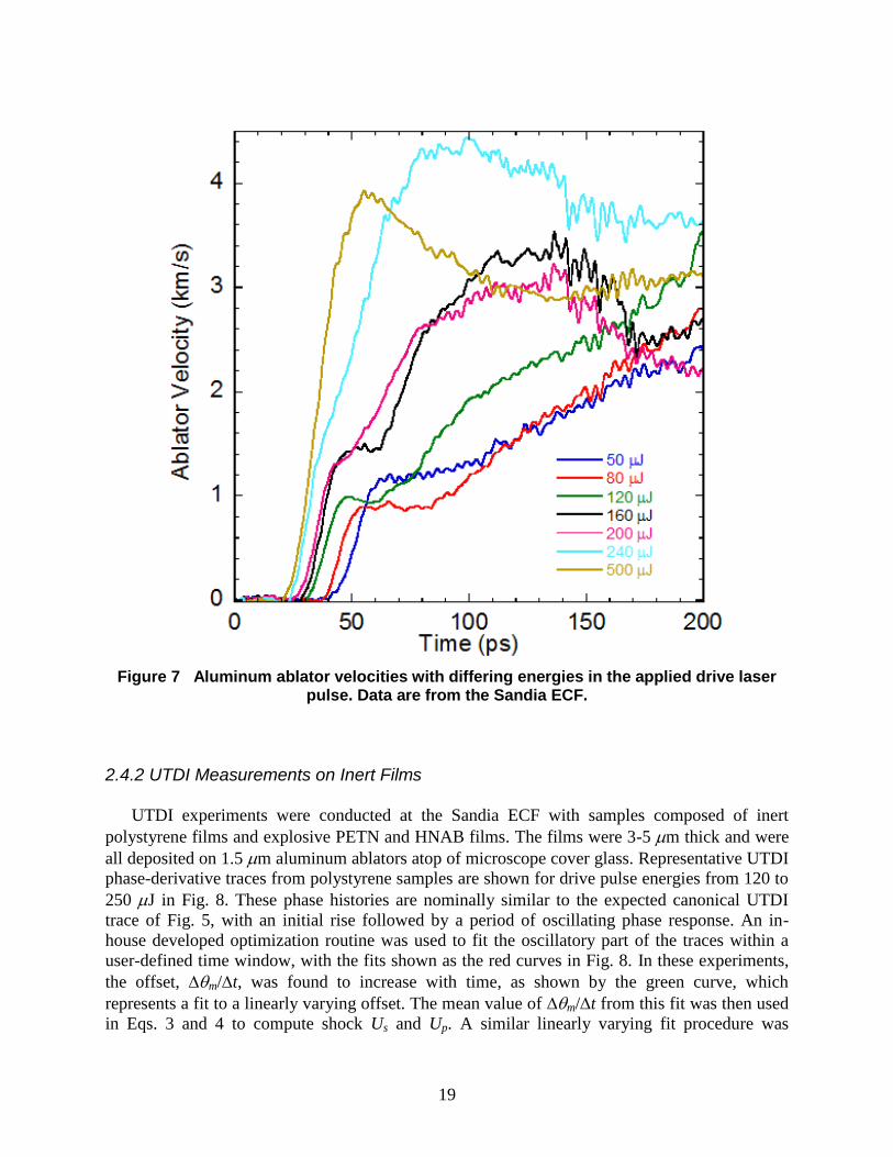
Figure 7 Aluminum ablator velocities with differing energies in the applied drive laser pulse.

Data are from the Sandia ECF. ..................................................................................................... 19

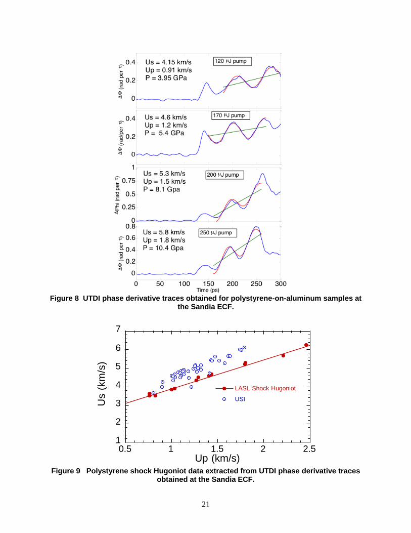
Figure 8 UTDI phase derivative traces obtained for polystyrene-on-aluminum samples at the

Sandia ECF. .................................................................................................................................. 21

Figure 9 Polystyrene shock Hugoniot data extracted from UTDI phase derivative traces

obtained at the Sandia ECF. .......................................................................................................... 21

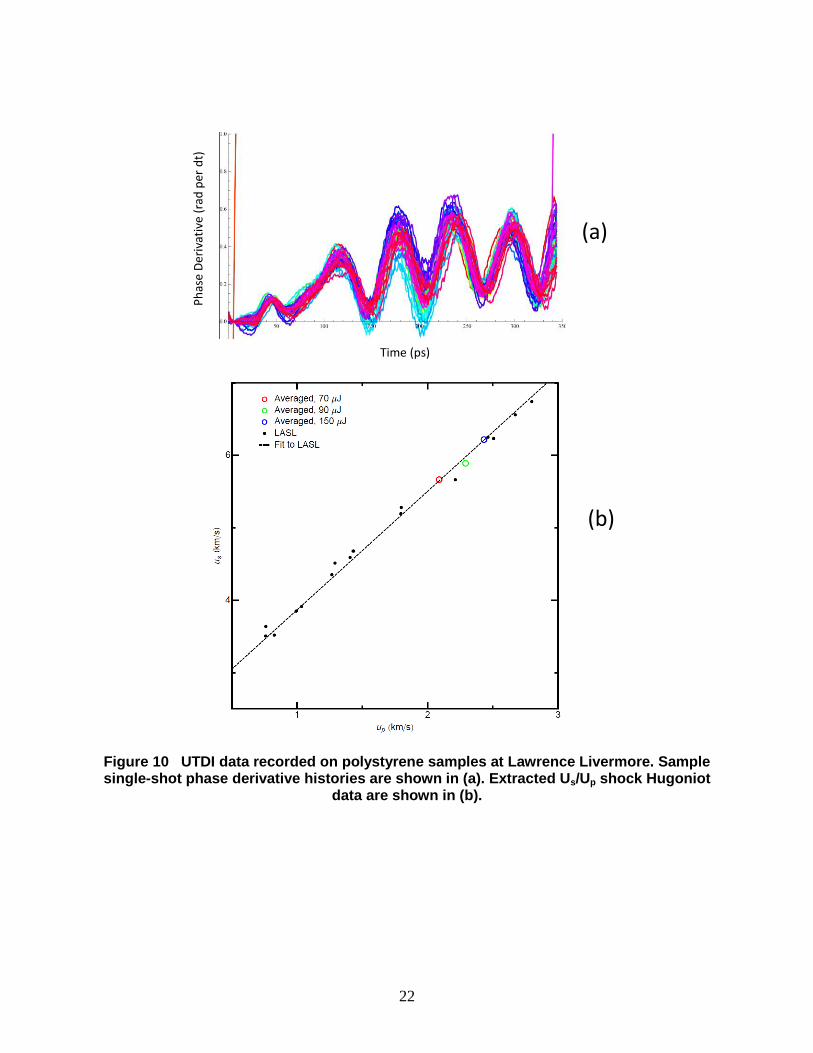
Figure 10 UTDI data recorded on polystyrene samples at Lawrence Livermore. Sample single-

shot phase derivative histories are shown in (a). Extracted Us/Up shock Hugoniot data are shown

in (b). ............................................................................................................................................. 22

Figure 11 UTDI phase derivative traces obtained for HNAB-on-aluminum samples at the

Sandia ECF. .................................................................................................................................. 24

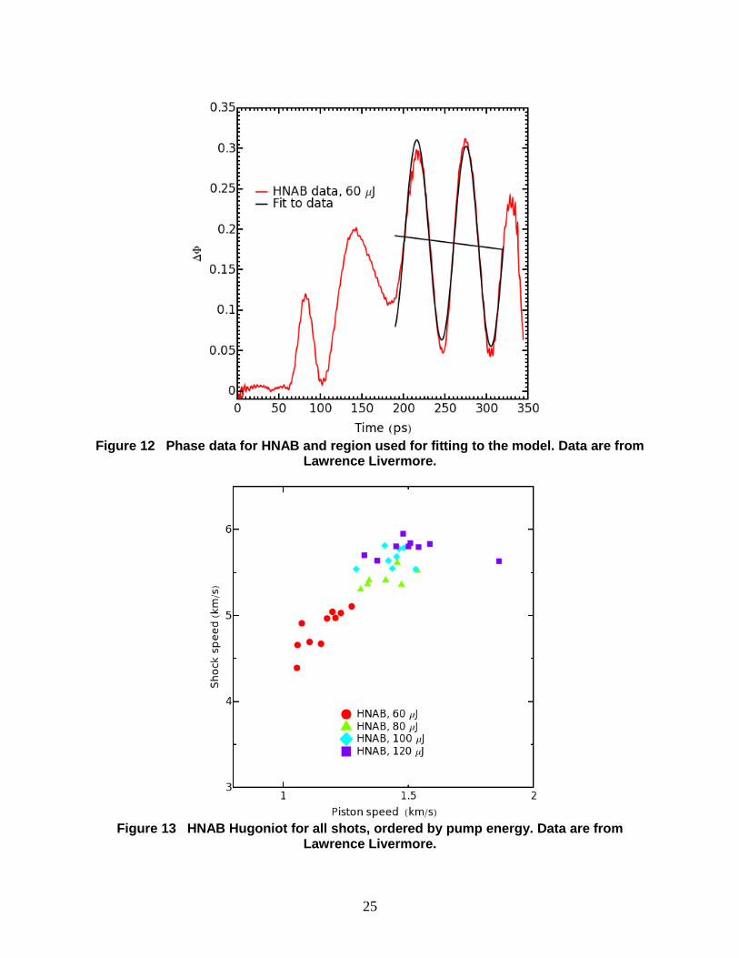
Figure 12 Phase data for HNAB and region used for fitting to the model. Data are from

Lawrence Livermore. .................................................................................................................... 25

Figure 13 HNAB Hugoniot for all shots, ordered by pump energy. Data are from Lawrence

Livermore. ..................................................................................................................................... 25

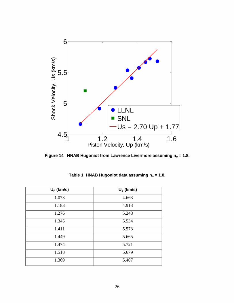
Figure 14 HNAB Hugoniot from Lawrence Livermore assuming no = 1.8................................ 26

7

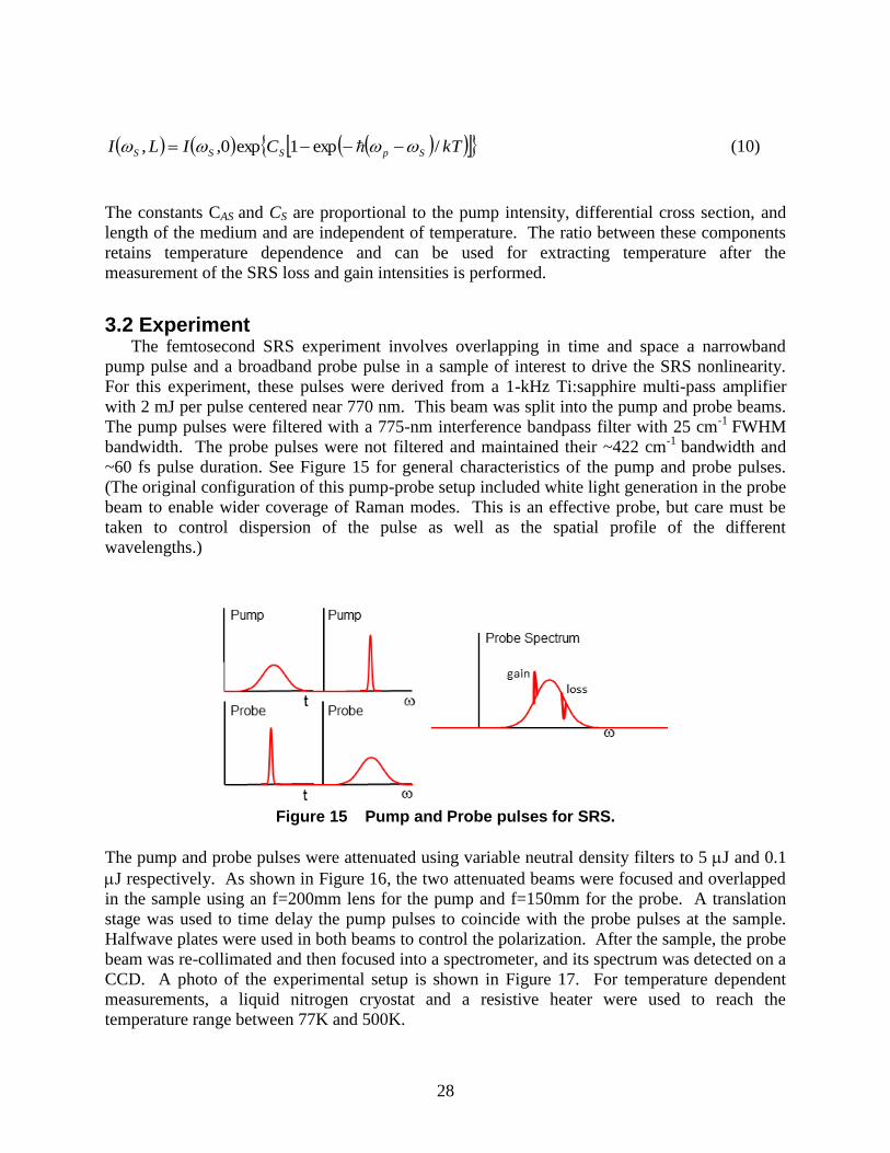
Figure 15 Pump and Probe pulses for SRS. ............................................................................... 28

Figure 16 Experimental setup for SRS. ...................................................................................... 29

Figure 17 a) Photo of experimental setup for SRS. b) Photo of quartz sample in cryostat. ..... 29

Figure 18 Raw SRS spectrum for quartz at 140 K...................................................................... 30

Figure 19 Raw a) anti-Stokes and b) Stokes SRS spectrum for quartz at 140 K. Line in red is

the fitting curve used to remove background signal arising from nonlinear effect. ..................... 30

Figure 20 Background subtracted a) anti-Stokes and b) Stokes SRS spectrum for quartz at 140

K. Background originating from pulse induced nonlinearities. ................................................... 31

Figure 21 Plot of SRS ratio as a function of temperature as predicted by theory for the 207 cm-1

mode of quartz. The different curves represent different levels of Raman gain generated in the

sample ........................................................................................................................................... 32

Figure 22 Plot of IAnti-Stokes as a function of temperature for the 207 cm-1

mode of quartz. The

red line is the numerical result for IAnti-Stokes. ................................................................................ 32

Figure 23 Plot of IStokes as a function of temperature for the 207 cm-1

mode of quartz. The red

line is the numerical result for IStokes. ............................................................................................ 33

Figure 24 Plot of SRS ratio as a function of temperature for the 207 cm-1

mode of quartz. The

red line is the numerical result for IStokes. ...................................................................................... 34

Figure 25 Experimental setup for broadband SRS. .................................................................... 36

Figure 26 a) Anti-Stokes and b) Stokes SRS spectra from liquid benzene (990 cm-1

mode) using

broadband SRS.............................................................................................................................. 36

Figure 27 a) Anti-Stokes and b) Stokes SRS spectra from 3-mm calcite sample (1091 cm-1

mode) using broadband SRS. ........................................................................................................ 37

Figure 28 SRS spectra from 3-mm calcite sample (1091 cm-1

mode) using broadband SRS. ... 38

Figure 29 Schematic of transient absorption experiment. Doubled, compressed output from

Ti:Sapphire amplifier is used to generate continuum in a CaF2 widow that extends into the UV

(400-300 nm) . The uncompressed output of the Ti:Sapphire amplifier (t ~ 150 ps FWHM) is

focused into an aluminum thin film to generate a shockwave that travels into the adjacent PETN

thin film. Changes in the UV probe spectrum are used to follow change in the HOMO/LUMO

gap of vapor deposited PETN under shock loading. Reference arm not used in preliminary

measurements (blocked). .............................................................................................................. 40

8

Figure 30 Schematic of transient absorption experiment using only 400nm pump (no

continuum). ................................................................................................................................... 41

Figure 31 2D and 1D images of continuum spectrum over a series of pump/probe delays.

Reference and post spectra averaged over 5 spectra. .................................................................... 43

Figure 32 Average UV continuum spectrum (blue) from 40 single-shots plotted with standard

deviation (black). .......................................................................................................................... 44

Figure 33 Intensity change of 400nm probe spectrum with pump delay (ps). ........................... 44

TABLES

Table 1 HNAB Hugoniot data assuming no = 1.8. ....................................................................... 26

9

1. INTRODUCTION

Despite its importance, a fundamental description of initiation in energetic materials has

eluded researchers for decades, in large part because ignition results from mechanical and

thermochemical mechanisms that are tightly coupled at extreme spatial and temporal scales of

order microns and picoseconds. Access to these extreme time and length scales under dynamic

loading conditions has, until recently, been restricted to simulations, and experiments to underpin

the relevant physics are sorely needed to provide model developers with an appropriate physical

foundation. The recent availability of femtosecond laser sources has opened the door to

fundamental experiments with the required extreme resolution, and well-controlled

measurements on the early time effects of shock drive are now possible.

This project represents a development effort to cultivate state-of-the-art tabletop diagnostic

tools for probing of energetic materials under dynamic shock loading. Efforts are focused on thin

films of both inert and energetic materials, which makes the experiments amenable to direct

laser-driven generation of shock waves and results in experimental conditions which are free of

many of personnel hazards associated with explosive operations. The report is centered around

three primary diagnostic-development efforts, each of which is highlighted independently in its

own chapter. Chapter 2 of this report is devoted to Ultrafast Time-Domain Interferometry

(UTDI) as well as methods for utilizing shaped picosecond laser pulses to impart shock drive

into the thin-film samples. UTDI is important because it characterizes the mechanical and shock

response of the film to the laser drive, providing shock characterization and boundary conditions

for any spectroscopic measurement of the material response. UTDI provides the additional

advantage of yielding shock Hugoniot data for materials, enabling tabletop Hugoniot

measurement capability. Chapter 3 is focused on the application of stimulated Raman scattering

(SRS) for thermometry. Temperature has proven to be a particularly difficult parameter to

measure in dynamic experiments. The SRS capability developed here has been demonstrated

with two different laser schemes, and results on static films are reported here. Chapter 4

concludes this report and is dedicated to the development of ultra-broadband absorption

spectroscopy schemes for characterization of explosive samples.

10

11

2. ULTRAFAST TIME DOMAIN INTERFEROMETY (UTDI)

2.1 UTDI Experimental Setup

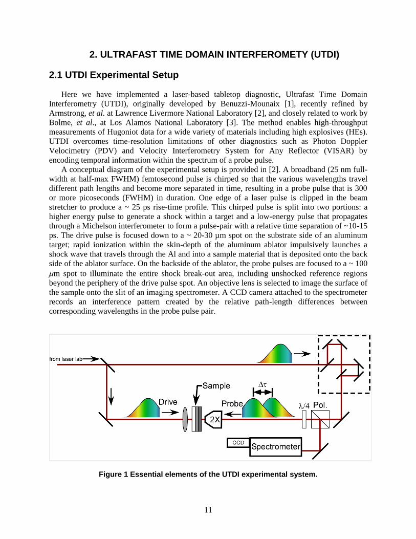
Here we have implemented a laser-based tabletop diagnostic, Ultrafast Time Domain

Interferometry (UTDI), originally developed by Benuzzi-Mounaix [1], recently refined by

Armstrong, et al. at Lawrence Livermore National Laboratory [2], and closely related to work by

Bolme, et al., at Los Alamos National Laboratory [3]. The method enables high-throughput

measurements of Hugoniot data for a wide variety of materials including high explosives (HEs).

UTDI overcomes time-resolution limitations of other diagnostics such as Photon Doppler

Velocimetry (PDV) and Velocity Interferometry System for Any Reflector (VISAR) by

encoding temporal information within the spectrum of a probe pulse.

A conceptual diagram of the experimental setup is provided in [2]. A broadband (25 nm full-

width at half-max FWHM) femtosecond pulse is chirped so that the various wavelengths travel

different path lengths and become more separated in time, resulting in a probe pulse that is 300

or more picoseconds (FWHM) in duration. One edge of a laser pulse is clipped in the beam

stretcher to produce a ~ 25 ps rise-time profile. This chirped pulse is split into two portions: a

higher energy pulse to generate a shock within a target and a low-energy pulse that propagates

through a Michelson interferometer to form a pulse-pair with a relative time separation of ~10-15

ps. The drive pulse is focused down to a ~ 20-30 µm spot on the substrate side of an aluminum

target; rapid ionization within the skin-depth of the aluminum ablator impulsively launches a

shock wave that travels through the Al and into a sample material that is deposited onto the back

side of the ablator surface. On the backside of the ablator, the probe pulses are focused to a ~ 100

m spot to illuminate the entire shock break-out area, including unshocked reference regions

beyond the periphery of the drive pulse spot. An objective lens is selected to image the surface of

the sample onto the slit of an imaging spectrometer. A CCD camera attached to the spectrometer

records an interference pattern created by the relative path-length differences between

corresponding wavelengths in the probe pulse pair.

Figure 1 Essential elements of the UTDI experimental system.

12

Extreme, picosecond-scale time resolution is achieved in UTDI measurements by encoding

time information into the frequency domain via the above-mentioned temporal chirp in the

stretched laser pulse. The structure of a typical chirped pulse is shown in Fig. 2. At left in Fig. 2

is as second-harmonic FROG (Frequency Resolved Optical Gate) trace, which displays the linear

dependence of the UTDI laser pulse wavelength with time. With this wavelength/time

characteristic, the spectral axis of the UTDI trace is readily converted to a high-resolution

picosecond time sweep. This wavelength/time conversion was used to estimate the time history

of the UTDI pulse from the directly measured pulse spectrum as shown at right in Fig. 2. Here,

the rise time of the pulse has been estimated at ~25 ps, based on the 10%-90% intensity points.

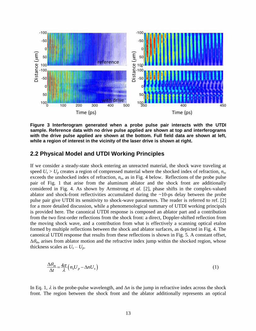
A sample UTDI trace obtained from a polystyrene-on-aluminum sample is shown in Figure

3. A reference interferogram from a static surface without shock drive is shown in at top, while

data from the same sample during with the laser drive applied are shown below. The vertical axis

represents a 1-D cut through the center of the pump-beam spot, with a resolution of 1.5 m/pixel.

Time is represented on the horizontal, where the resolution in the measurement is 10 ps. In each

case, the full-field interferogram is shown on the left, and “zoomed in” results that highlight the

impact of laser drive at time t = 350-450 ps are shown on the right. The fringes in the reference

data are essentially straight, while the results with laser drive reveal fringe curvature as a result

of phase shift that is accumulated within the delay, t, between the probe laser pulses. Phase

shifts in the UTDI data are analyzed to yield the ablator or piston velocity (Up), the shock

velocity (Us), and the shocked index of refraction (ns) in the material. UTDI measurements can

then be performed over a range of laser drive conditions to vary shock drive pressure and extract

Us-Up Hugoniot data according to the physical model which describes the canonical USI

response that is presented next.

Figure 2 Characteristics of temporally chirped laser pulse for UTDI measurements. Second-harmonic FROG trace showing the time dependence of the laser wavelength that encodes time into the spectral domain (left). Extracted laser pulse shape with rapid ~25 ps rise.

13

Figure 3 Interferogram generated when a probe pulse pair interacts with the UTDI sample. Reference data with no drive pulse applied are shown at top and interferograms with the drive pulse applied are shown at the bottom. Full field data are shown at left, while a region of interest in the vicinity of the laser drive is shown at right.

2.2 Physical Model and UTDI Working Principles

If we consider a steady-state shock entering an unreacted material, the shock wave traveling at

speed Us > Up creates a region of compressed material where the shocked index of refraction, ns,

exceeds the unshocked index of refraction, no, as in Fig. 4 below. Reflections of the probe pulse

pair of Fig. 1 that arise from the aluminum ablator and the shock front are additionally

considered in Fig. 4. As shown by Armstrong et al. [2], phase shifts in the complex-valued

ablator and shock-front reflectivities accumulated during the ~10-ps delay between the probe

pulse pair give UTDI its sensitivity to shock-wave parameters. The reader is referred to ref. [2]

for a more detailed discussion, while a phenomenological summary of UTDI working principals

is provided here. The canonical UTDI response is composed an ablator part and a contribution

from the two first-order reflections from the shock front: a direct, Doppler-shifted reflection from

the moving shock wave, and a contribution from what is effectively a scanning optical etalon

formed by multiple reflections between the shock and ablator surfaces, as depicted in Fig. 4. The

canonical UTDI response that results from these reflections is shown in Fig. 5. A constant offset,

m, arises from ablator motion and the refractive index jump within the shocked region, whose

thickness scales as Us – Up.

4ms p sn U nU

t

(1)

In Eq. 1, is the probe-pulse wavelength, and n is the jump in refractive index across the shock

front. The region between the shock front and the ablator additionally represents an optical

14

etalon of time-varying thickness, whose complex-valued reflectivity varies periodically as the

shocked region thickness passes through integer-multiples of the probe light’s optical path. The

reflectivity is then expected to have a phase contribution which varies periodically, with period , as

2s p

s

U Un . (2)

This canonical response is then characterized in terms of an initial rise to the phase offset m,

and an oscillatory part with period, , and amplitude, , which can be extracted from a fit to the

oscillatory portion of the measured phase-derivative response. Armstrong’s detailed analysis [2]

relates these measured phase shift parameters to shock wave properties.

(3)

(4)

(5)

Once Us and Up are determined, the shock pressure can be determined from the Rankine-

Hugoniot jump conditions across a steady shock wave as

. (6)

2

4 0 tnU m

s

s

mP

n

n

tnU 0

0

12

4

t

nnns

2

00

15

Figure 4 Physical model to describe reflections from the shock front and ablator surface.

Only the first-order reflections from the shock front and ablator are considered in the analysis.

Figure 5 Canonical UTDI trace of phase accumulated per unit of time equal to the probe pair separation. The offset (Δθm), amplitude (δ), and period (τ) are measured quantities

used to determine Us, Up, and ns.

AblatorShockedmaterial

Unshockedmaterial

UsUp

ns n0P

has

e p

er

tim

e (r

ad/p

s)

Time (ps)

Δθm

δ

τ

16

2.3 Sandia UTDI Experiment

The experimental apparatus constructed at the Sandia Explosive Components

Facility (ECF) is similar to that used in previous work [2], and with key elements as shown in

Fig 1. A commercial Ti:Sapphire amplifier (KM Labs Wyvern) provides 4-mJ pulses of 42-fs

duration at 1-kHz repetition rate. The amplifier output spectrum is centered near 790 nm, with a

bandwidth of 25 nm (FWHM). A user-selectable portion of the ~170-ps regenerative amplifier

output energy is extracted before compression and further stretched in an off-design external

grating compressor, so that the blue edge of the spectrum leads the red. A fast time-domain rise

is added to the pulse by clipping the dispersed spectrum within the compressor. Previous work

[2-10] using an external stretcher, produced 10- to 20-ps rise shock waves in aluminum films. In

the “overcompressed” pulse-shaper design used here, lack of a true Fourier plane in our external

compressor may result in a more gradual rise to the clipped spectrum and time-domain pulse.

The bandwidth-clipped and stretched pulse is relayed to the sample in the arrangement shown

in Fig. 1. The majority of the pulse energy is delivered to the pump (shock drive) beam directed

onto the back side of the samples; 2-m thick aluminum films deposited on a glass substrate

were utilized either in bare condition or with an inert (polystyrene/sylgard) or explosive (HNAB)

stacked onto the ablator. The pump beam is focused at a numerical aperture (NA) ~0.03 using a f

= 150-mm convex lens. The pump then focuses through the glass substrate to a ~20-30-m spot

at the back surface of the aluminum ablator, where the momentum exchange from the formation

of laser-induced plasma drives a shock wave into the film. A small fraction of the pulse energy is

split via a Michelson-type interferometer, where a delay is introduced to form the collinear

probe-pulse pair that is directed to the sample through a polarizing cube with circular

polarization imparted by a quarter-wave plate. Nominal delay between the probe pulses is ~10-

15 ps, as determined from the fringe spacing in the UTDI interferograms. The probe-pulse pair is

weakly focused at normal incidence onto the sample through the combined effect of a 2×

microscope objective of 0.07 NA and a f = 500-mm lens placed in the probe beam path.

Introduction of the 500-mm lens permits proper imaging of the sample plane with a probe that is

only weakly focused to ~100-m, 3× larger than the pump-beam spot that is centered within the

probe. Back-reflected probe-beam energy is collected through the microscope objective and

rejected by the polarizer-waveplate pair onto the entrance slit of a 0.3-m grating spectrograph,

where the pulses are spectrally dispersed and combined at the face of a CCD camera placed at

the spectrometer focal plane.

The sample plane during a laser-drive experiment is depicted in Fig. 6 [2], where the

deformation of the laser-driven ablator forms a “piston interface” behind an expanding shock

front. For the conditions of a “typical” UTDI experiment described here, Armstrong [4] has

shown that the radius of curvature of the shock front is large compared to the sample thickness,

so that 1-D shock conditions exist locally within the film. We note that our experiment measures

the piston speed, not the particle speed just behind shock front, but it has been shown in previous

work [6] that, by assuming the particle speed is the same as the measured piston speed, the

measured shockwave speed will correspond to the known Hugoniot to better than 2% accuracy

[6, 11].

An in-house built MATLAB code has been constructed to extract the phase accumulation

over the probe pair delay on a row-by-row basis within the shocked region by subtracting the

complex-valued Fourier transforms of the shocked-region row data from reference regions taken

outside of the shock-drive zone and in reference frames taken just before the laser-drive

17

experiments, as shown previously in Fig. 3. Inverse transform of these results yields time-

dependent phase derivatives of the type shown canonically in Fig. 5. The resulting phase fields

are then fit to model Eqs. 3-5 to extract shock parameters.

Figure 6 A schematic cross section of the experiment at the sample [2].

18

2.4 UTDI Results

2.4.1 Shock Breakout Measurements on Bare Aluminum Films Measurements were initially performed on bare aluminum films to characterize the response

of both the UTDI setup and the performance of the picosecond laser-drive for shock wave

generation. Without a sample film, the velocity of the bare aluminum ablator, Ua, during shock

breakout is related to the UTDI phase derivative by,

4aUt

. (7)

Representative ablator velocity histories recorded in the ECF facilities in building 905 during

shock breakout are shown in Fig. 7, where velocity traces for different drive pulse energies are

shown. The velocity data are extracted from the region in the center of the drive pulse, where

maximum surface displacement occurs. The data are consistent with very strong elastic

precursors, as identified by Crowhurst et al. [11] in their UTDI investigation of the effect

material thickness on direct laser drive. At drive pulse energies below ~500 J, the ablator

response is characterized by an initial rise to a velocity plateau of Ua = 1-1.5 km/s, as a result of

strong, but elastic deformation. The elastic wave is then followed by a second, more gradual rise

to a higher speed resulting from a follow-on plastic deformation. As the drive pulse energy is

increased, the duration of the velocity plateau following the elastic wave shortens and the

maximum ablator velocity attained during the second, plastic wave increases to Ua ~ 4 km/s.

Eventually, the drive pulse is sufficiently intense that the plastic wave overtakes the elastic

precursor, resulting in single plastic deformation whose risetime is 20-30 ps. It is at this drive

energy that a shock wave is present during ablator breakout.

The 500-J critical drive pulse energy identified here is significantly larger than observed in

previous picosecond laser-drive experiments [2-12], where drive energies of only 50-100 J

were sufficient to achieve plastic shock breakout in bare aluminum layers. At this time, we

believe the reason for this is the stretcher design employed, which lacks a Fourier plane where

the spectral elements are in focus. Clipping the laser bandwidth with out-of-focus spectral

elements likely results in a more gradual initial rise in the drive pulse, so that more energy is

needed to achieve steady shock conditions. This will become a factor in later investigations with

inert and explosive material samples deposited on the aluminum layer.

19

Figure 7 Aluminum ablator velocities with differing energies in the applied drive laser

pulse. Data are from the Sandia ECF.

2.4.2 UTDI Measurements on Inert Films

UTDI experiments were conducted at the Sandia ECF with samples composed of inert

polystyrene films and explosive PETN and HNAB films. The films were 3-5 m thick and were

all deposited on 1.5 m aluminum ablators atop of microscope cover glass. Representative UTDI

phase-derivative traces from polystyrene samples are shown for drive pulse energies from 120 to

250 J in Fig. 8. These phase histories are nominally similar to the expected canonical UTDI

trace of Fig. 5, with an initial rise followed by a period of oscillating phase response. An in-

house developed optimization routine was used to fit the oscillatory part of the traces within a

user-defined time window, with the fits shown as the red curves in Fig. 8. In these experiments,

the offset, m/t, was found to increase with time, as shown by the green curve, which

represents a fit to a linearly varying offset. The mean value of m/t from this fit was then used

in Eqs. 3 and 4 to compute shock Us and Up. A similar linearly varying fit procedure was

20

employed by Armstrong et al. in their UTDI measurements on shocked H2O2 [6], where

unsteady piston speeds resulting from shock-induced chemistry resulted in a time-dependent

phase offset. Here, we suspect that the observed time dependence in m/t is a result of

unsteady wave propagation in the experiments as a result of the above-mentioned slow rise in the

picosecond shock drive pulse. We conducted additional experiments with drive energies in

excess of 500 J in an effort to reach the steady shock behavior observed in the bare ablator

results of Fig. 7. However, the quality of the UTDI traces at these high drive energies on the

polystyrene samples was not sufficient for analysis.

Fitted (Us, Up) data from polystyrene data similar to that of Fig. 8 were used to construct a

Hugoniot curve for unreacted polystyrene. The results are shown in Fig. 9, where data from the

SNL ECF lab are plotted as open, blue circles and compared to historical data for “fully dense”

polystyrene compiled by Marsh [13]. The UTDI measurements from SNL lie ~10-12 % above

the historical polystyrene Hugoniot. As a check, UTDI measurements on similar polystyrene

films were provided from Lawrence Livermore [14], with their results shown in Fig. 10. In Fig.

10a, representative UTDI phase histories are plotted, where the phase offset in the oscillatory

portion of the trace appears approximately constant, in contrast to the results from Sandia shown

in Fig. 8, suggesting a more steady shock drive in the Livermore experiments. Shock-Hugoniot

data extracted from traces like those in Fig. 10a are shown in Fig. 10b, where three UTDI results

are plotted as open, colored circles against the same historical data from Marsh shown in Fig. 9.

In this case, the Livermore data reveal that the UTDI technique is capable of faithfully

reproducing accepted shock Hugoniot data for a well-understood inert material.

Departure of the Sandia UTDI data from historical gas-gun data and Livermore UTDI results

is likely a result of unsteady wave propagation in the polystyrene film, such that the speed of the

post-shock material and the measured piston velocity do not equilibrate during the experiment.

The consistently upward slope in the UTDI phase derivative data of Fig. 8 suggest that the wave

speed is consistently increasing throughout the measurement.

21

Figure 8 UTDI phase derivative traces obtained for polystyrene-on-aluminum samples at

the Sandia ECF.

Figure 9 Polystyrene shock Hugoniot data extracted from UTDI phase derivative traces

obtained at the Sandia ECF.

1

2

3

4

5

6

7

0.5 1 1.5 2 2.5

LASL Shock Hugoniot

USI

Us (

km

/s)

Up (km/s)

22

Figure 10 UTDI data recorded on polystyrene samples at Lawrence Livermore. Sample single-shot phase derivative histories are shown in (a). Extracted Us/Up shock Hugoniot

data are shown in (b).

Ph

ase

Der

ivat

ive

(rad

per

dt)

Time (ps)

(a)

(b)

23

2.4.3 UTDI Measurements on HNAB films

Hexanitroazobenzene (HNAB) is an energetic material with properties that make it a model

system to study the effects of microstructure on initiation. HNAB can be vapor-deposited as a

fully dense amorphous film. If kept at room temperature, it crystallizes into a dense film (99.4%

TMD) with nanometer-scale pores [15]. In the amorphous state, it shares some properties with

liquid explosives: it has an isotropic molecular network (no long range order) and lacks micron-

scale pores that can serve to nucleate shock-induced chemical initiation. Unlike liquid

explosives, solid explosives like HNAB form much stronger intermolecular bonds. Detonation

studies may be conducted on crystalline and amorphous HNAB to elucidate how pores and

molecular ordering affect the shock initiation threshold. The material we probed was comprised

of the HNAB II polymorph whose indices of refraction, required for UTDI analysis, vary with

crystal orientation from 1.5 to 1.8 [16]. The films are randomly-oriented polycrystals so the

average refractive index should lie somewhere between those two values. Here we used 1.8 for

the index of refraction. UTDI experiments were performed on HNAB films at both the Sandia

ECF and at Lawrence Livermore. All HNAB films were fabricated at Sandia.

UTDI phase-derivative traces acquired at Sandia are shown in Fig. 11, with fits to the

oscillatory portion of the trace displayed in red and the linear fit to the phase offset shown in

green. These Sandia experiments were conducted with constant energy in the drive laser pulse

near 500 J, and the phase offset during the fitted portions oscillatory phase of these traces

appears to be improved over the polystyrene results shown in Fig. 8. The extracted shock

Hugoniot parameters display Us = 5.1 − 5.5 km/s with Up = 0.92 – 1.2 km/s, with an average

value of (Us, Up) = (5.2, 1.1) km/s. A representative HNAB UTDI history obtained a Lawrence

Livermore is shown in Fig. 12. The fitted oscillatory part and phase offset reveal that conditions

during the Livermore experiments were not perfectly steady.

UTDI-determined shock Hugoniot data for HNAB are presented in Fig. 13. The results were

obtained using an unshocked index of refraction of no = 1.8, as index measurements for the as-

deposited films were not available. The density of HNAB was taken to be 1.750 g/cm3 as

measured from flotation in an aqueous barium perchlorate solution [17]. The data seem to lie

upon a line except for a single outlier at the highest piston velocity. The plot of phase data for

this point was not as well-behaved as the others, so it is likely that a steady shock was not

present, and thus, the physical model used to derive Eqs. 3-5 was not satisfied. This single outlier

was eliminated, we then ordered all the remaining data points by piston velocity, binned them in

groups of 5, and averaged the Us and Up values by bin to create a Hugoniot plot with less scatter,

as shown in Fig. 14, with tabular data provided in Table 1. Both data from Livermore and the

four-shot averaged result from Sandia are included on the plot. A linear fit to the Livermore data

results in an HNAB shock Hugoniot of Us = 2.70 + 1.77 Up. The result from Sandia lies 10%

above this Hugoniot curve, similar to the polystyrene results presented above, although the

reason for the discrepancy here could very well result from changes to the morphology of the

HNAB films with time, which could result in changes to their shock response, it is likely that the

form of the shock drive pulse plays a role in the discrepancy.

24

Figure 11 UTDI phase derivative traces obtained for HNAB-on-aluminum samples at the

Sandia ECF.

25

Figure 12 Phase data for HNAB and region used for fitting to the model. Data are from

Lawrence Livermore.

Figure 13 HNAB Hugoniot for all shots, ordered by pump energy. Data are from

Lawrence Livermore.

26

Figure 14 HNAB Hugoniot from Lawrence Livermore assuming no = 1.8.

Table 1 HNAB Hugoniot data assuming no = 1.8.

UP (km/s) US (km/s)

1.073 4.663

1.183 4.913

1.276 5.248

1.345 5.534

1.411 5.573

1.449 5.665

1.474 5.721

1.518 5.679

1.369 5.407

1 1.2 1.4 1.64.5

5

5.5

6

Piston Velocity, Up (km/s)

Sho

ck V

elo

city,

Us (

km

/s)

LLNL

SNL

Us = 2.70 Up + 1.77

27

3. STIMULATED RAMAN SCATTERING AS A TEMPERATURE PROBE

3.1 Introduction Temperature is a quantity that impacts kinetics of physical and chemical processes, and yet it

is often not measured in solids due to its difficulty. In order to advance development of detailed

models for shock induced initiation with proper treatment of molecular-level reactions,

temperature must be extracted and provided as support data. For the fundamental description of

ultrafast shock responses in energetic materials, it is important to have means for access to

temperature at short time scales (~ps) over small volumes (~m3) as ignition mechanisms may

depend on ultrafast energy transfers and complex microstructures within the material.

A number of techniques have been used to measure temperature in the gas phase using

Raman techniques such as spontaneous Raman scattering and coherent anti-Stokes Raman

scattering [18]. But some of these techniques have limitations for temperature measurement in

small-volume solids. For example, in spontaneous Raman spectroscopy, the scattering rate is so

low that long acquisition time are required and background signals could obscure spectral

features. CARS approaches require use of models which are tractable for gases, but would be

difficult for complex solids.

Femtosecond stimulated Raman scattering offers a method of measuring temperature in

solids [19, 20]. This technique is analogous to the spontaneous Raman method of using anti-

Stokes to Stokes signal ratio to extract vibrational temperature. The advantage of femtosecond

SRS is that the scattering rate is orders of magnitude larger than that for spontaneous Raman

scattering. This offers an opportunity to measure temperature in small-volume solids with short

integration times. As an added benefit, the phase-matched output in the former allows for

rejection of background fluorescence for higher signal-to-noise ratio. In contrast to CARS, the

SRS measurement relies simply on the anti-Stokes to Stokes signal ratio and is independent of

material parameters. The analysis therefore is simplified and involves a fitting routine to the data

set as opposed to model development.

SRS occurs when pump and probe pulses overlap in time and space within a medium

characterized by

. SRS is generally described as an exponential amplification of the probe

pulse in the presence of the pump pulse in a material with differential cross section for Raman

scattering as indicated in the expression below.

GLILI probeSRS exp0 , where pumpIG

2. (8)

The differential cross section can be written in terms of the phonon thermal population and when

accounted for in the SRS signal intensity for the anti-Stokes (loss) and Stokes (gain)

components, the signal expressions can be written respectively as [19]:

kTCILI ASpASASAS /exp1exp)0,(, (9)

28

kTCILI SpSSS /exp1exp0,, (10)

The constants CAS and CS are proportional to the pump intensity, differential cross section, and

length of the medium and are independent of temperature. The ratio between these components

retains temperature dependence and can be used for extracting temperature after the

measurement of the SRS loss and gain intensities is performed.

3.2 Experiment The femtosecond SRS experiment involves overlapping in time and space a narrowband

pump pulse and a broadband probe pulse in a sample of interest to drive the SRS nonlinearity.

For this experiment, these pulses were derived from a 1-kHz Ti:sapphire multi-pass amplifier

with 2 mJ per pulse centered near 770 nm. This beam was split into the pump and probe beams.

The pump pulses were filtered with a 775-nm interference bandpass filter with 25 cm-1

FWHM

bandwidth. The probe pulses were not filtered and maintained their ~422 cm-1

bandwidth and

~60 fs pulse duration. See Figure 15 for general characteristics of the pump and probe pulses.

(The original configuration of this pump-probe setup included white light generation in the probe

beam to enable wider coverage of Raman modes. This is an effective probe, but care must be

taken to control dispersion of the pulse as well as the spatial profile of the different

wavelengths.)

Figure 15 Pump and Probe pulses for SRS.

The pump and probe pulses were attenuated using variable neutral density filters to 5 J and 0.1

J respectively. As shown in Figure 16, the two attenuated beams were focused and overlapped

in the sample using an f=200mm lens for the pump and f=150mm for the probe. A translation

stage was used to time delay the pump pulses to coincide with the probe pulses at the sample.

Halfwave plates were used in both beams to control the polarization. After the sample, the probe

beam was re-collimated and then focused into a spectrometer, and its spectrum was detected on a

CCD. A photo of the experimental setup is shown in Figure 17. For temperature dependent

measurements, a liquid nitrogen cryostat and a resistive heater were used to reach the

temperature range between 77K and 500K.

29

Figure 16 Experimental setup for SRS.

The samples used in the experiments were crystalline calcite and quartz. For calcite (100),

the sample was 1 mm in thickness and the observed Raman modes were located at 155 cm-1

and

282 cm-1

. The quartz sample was 1.5 mm in thickness and the Raman modes were measured at

147 cm-1

and 207 cm-1

[21].

Figure 17 a) Photo of experimental setup for SRS. b) Photo of quartz sample in cryostat.

The acquisition sequence consisted of recording the SRS probe on the CCD with adequate

SNR with the pump on and pump off. The SRS loss and gain spectra were obtained by

subtracting the pump-off spectrum from the pump-on spectrum and normalizing with respect to

the pump-off spectrum.

3.3 Measurement Results Figure 18 shows the SRS spectrum for crystalline quartz measured at 140 K. The pump-on

and pump-off spectra were subtracted and then normalized to generate this plot. With the

narrowband pump centered near 775 nm, the 147 cm-1

Raman mode appears at 766 nm and 784

nm as a negative anti-Stokes signal and positive Stokes signal respectively. The 207 cm-1

Raman

mode shows up near 763 nm and 787 nm. The signal-to-noise ratio was adequate to extract loss

and gain signal intensities. For this particular plot, 500 pulses were integrated on the CCD.

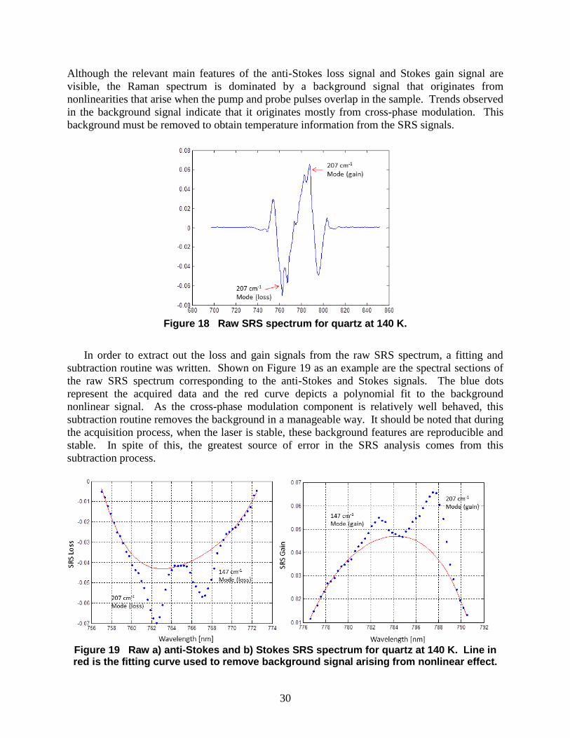
30

Although the relevant main features of the anti-Stokes loss signal and Stokes gain signal are

visible, the Raman spectrum is dominated by a background signal that originates from

nonlinearities that arise when the pump and probe pulses overlap in the sample. Trends observed

in the background signal indicate that it originates mostly from cross-phase modulation. This

background must be removed to obtain temperature information from the SRS signals.

Figure 18 Raw SRS spectrum for quartz at 140 K.

In order to extract out the loss and gain signals from the raw SRS spectrum, a fitting and

subtraction routine was written. Shown on Figure 19 as an example are the spectral sections of

the raw SRS spectrum corresponding to the anti-Stokes and Stokes signals. The blue dots

represent the acquired data and the red curve depicts a polynomial fit to the background

nonlinear signal. As the cross-phase modulation component is relatively well behaved, this

subtraction routine removes the background in a manageable way. It should be noted that during

the acquisition process, when the laser is stable, these background features are reproducible and

stable. In spite of this, the greatest source of error in the SRS analysis comes from this

subtraction process.

Figure 19 Raw a) anti-Stokes and b) Stokes SRS spectrum for quartz at 140 K. Line in red is the fitting curve used to remove background signal arising from nonlinear effect.

31

When the baseline correction is made, the loss and gain spectra appear as those in Figure 20.

Here, the data from Figure 19 are directly processed, and the paired 147 cm-1

and 207 cm-1

Raman modes are clearly observed as negative anti-Stokes signals and positive Stokes signals.

Figure 20 Background subtracted a) anti-Stokes and b) Stokes SRS spectrum for quartz

at 140 K. Background originating from pulse induced nonlinearities.

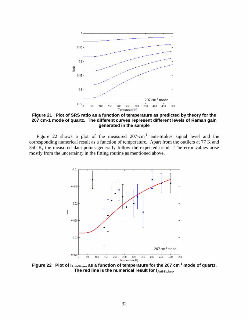
3.4 Discussion For demonstration of the thermometric capabilities of the femtosecond SRS method, SRS

data sets were measured and analyzed over the temperature range of 77K to 500K. Plotted in

Figure 21 is a set of curves representing the SRS ratio as a function of temperature. These

curved were generated by evaluating the anti-Stokes to Stokes signal ratio from the expressions

given for loss and gain above. The five curves correspond to five different gain values assigned

to the SRS interaction. The lowest curve has the highest gain, and it shows that over the

temperature range of 100K to 500K, higher temperature sensitivity is achieved at higher gain

levels. These numerical results will be compared to measured data to verify the predictive

matching of temperature trends.

32

Figure 21 Plot of SRS ratio as a function of temperature as predicted by theory for the 207 cm-1 mode of quartz. The different curves represent different levels of Raman gain

generated in the sample

Figure 22 shows a plot of the measured 207-cm-1

anti-Stokes signal level and the

corresponding numerical result as a function of temperature. Apart from the outliers at 77 K and

350 K, the measured data points generally follow the expected trend. The error values arise

mostly from the uncertainty in the fitting routine as mentioned above.

Figure 22 Plot of IAnti-Stokes as a function of temperature for the 207 cm-1 mode of quartz.

The red line is the numerical result for IAnti-Stokes.

33

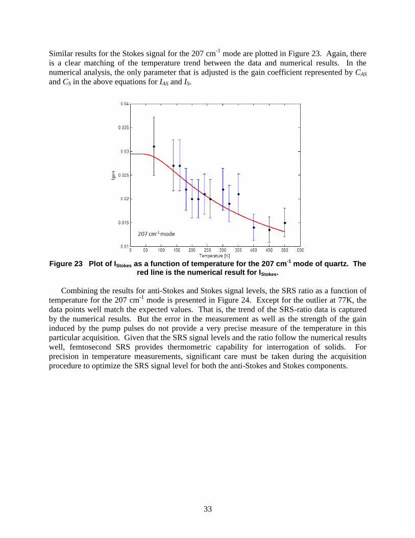
Similar results for the Stokes signal for the 207 cm-1

mode are plotted in Figure 23. Again, there

is a clear matching of the temperature trend between the data and numerical results. In the

numerical analysis, the only parameter that is adjusted is the gain coefficient represented by CAS

and CS in the above equations for IAS and IS.

Figure 23 Plot of IStokes as a function of temperature for the 207 cm-1 mode of quartz. The

red line is the numerical result for IStokes.

Combining the results for anti-Stokes and Stokes signal levels, the SRS ratio as a function of

temperature for the 207 cm-1

mode is presented in Figure 24. Except for the outlier at 77K, the

data points well match the expected values. That is, the trend of the SRS-ratio data is captured

by the numerical results. But the error in the measurement as well as the strength of the gain

induced by the pump pulses do not provide a very precise measure of the temperature in this

particular acquisition. Given that the SRS signal levels and the ratio follow the numerical results

well, femtosecond SRS provides thermometric capability for interrogation of solids. For

precision in temperature measurements, significant care must be taken during the acquisition

procedure to optimize the SRS signal level for both the anti-Stokes and Stokes components.

34

Figure 24 Plot of SRS ratio as a function of temperature for the 207 cm-1 mode of quartz.

The red line is the numerical result for IStokes.

The following are some considerations that will need to be addressed in order to increase the

precision on the SRS measurement and analysis.

Increasing the gain of SRS increases the temperature sensitivity of the SRS ratio

curve. This gain increase can be achieved with increased pump pulse energies.

But there is a limit to this as increased pump energies induce significant

background nonlinear signals which distort the SRS spectrum. When the pump

energy is increased to high levels, white light is generated within the sample

making the SRS method intractable.

Pump induced nonlinearities such as cross phase modulation need to be

minimized by controlling the pump energy, sample thickness, and timing between

the pump and probe pulses. The modulation observed in the SRS spectrum

showed dependence on peak intensities and time delays. When the source laser is

stable, these modulations are stable. For full analysis of the background

contribution to the SRS spectrum, a full treatment of the field propagation within

the material will have to be carried out.

Spatial, spectral, and temporal characteristics of the pump and probe pulses need

to be well examined. For an ideal SRS experiment, the spatial mode of the beams

should be well characterized so that intensity values could be determined

precisely over the entire bandwidth. The spectral and temporal properties of the

probe pulse should be such that the arrival time of the different wavelengths is

within tolerance of the measurement. During the experiment, care must be taken

to ascertain that the anti-Stokes and Stokes signals are optimized simultaneously

and that the peak signal levels are occurring at the same delay.

Data acquisition needs to be set up so that the pump-on and pump-off spectra can

be captured quickly so that impact of laser jitter could be minimized.

A balance must be struck on sample thickness as higher thickness will generate

more SRS signal as well as the background nonlinearity. For studies on thin

35

films, unless a material has unusually high optical response for SRS, SNR based

on few hundred shots with ~micro Joules of pump pulse energy on a less than 100

m sample would be difficult because of the achievable signal levels.

SRS enhancement may be achieved through electronic enhancement by operating

the experiment our in the shorter wavelength region. The pump could be

generated using second harmonic and white light near the pump wavelength could

be used for the probe. The drawback to this approach is the potential for

increased noise in the white light.

The original plan for SRS in this project was to use SRS thermometry to measure

temperature in thin films of energetic materials. We explored this option, but there were

challenges as follows.

For samples such as PETN, the surface and volume quality of the sample made

intensity delivery too difficult. Due to the surface and volume roughness, the

pump and probe pulses diffusely scattered making the measurement

unmanageable.

For samples such as HNAB and HNS, the SRS response was too weak on samples

that were 10s of microns in thickness. In addition, the nonlinear response from

the substrate dominated the probe signal.

Sample burning was an issue on all film samples when the pump energy was

increased to improve SRS response.

In order to increase the interaction length, pressed pellets of PETN, HNAB, and

HNS were examined. But these samples, as with the films, did not allow for clean

transmission of the probe beam. There was cleaner transmission in HNS, but the

SRS response was too weak.

As with the quartz and calcite samples, the nonlinear signals were generated when

the pump and probe pulses overlapped in the sample.

Based on this study, it does not appear that SRS could be used directly on dynamically driven

energetic materials that are very thin and require single-shot acquisition. But if the laser or

mechanical shock drive could be extended so that the sample thickness could be increased, there

may be opportunity to take advantage of femtosecond SRS.

3.5 Broadband SRS Using OPA + SHG and other considerations In order to improve upon the pump-probe SRS technique, a setup using the second harmonic

of an optical parametric amplifier (OPA) for the probe pulses was built. This allowed for

broader spectral coverage, improved amplitude and timing control of the anti-Stokes and Stokes

probe pulses, and use of reference spectra during acquisition. The schematic of the setup is in

Figure 25.

36

Figure 25 Experimental setup for broadband SRS.

The basic concept of the SRS experiment is the same, but now, the probe is composed of two

separate pulses with one of them spectrally aligned for the anti-Stokes probe and the other for the

Stokes probe. These pulses are generated by sending 1-mJ, 770-nm pulses into the OPA for IR

signal and idler outputs (~10s of micro Joules). These OPA pulses are then frequency doubled in

BBO nonlinear crystals to produce the SRS probe pulses. In order to generate reference pulses

which are used to normalize the probe spectrum and to remove effects from variations in optical

and detector responses, each of the probe pulse is split and spatially and temporally separated.

These four probe pulses are then combined with the spectrally narrowed pump pulse at the

sample as in the earlier setup. The signal probe pulses and reference probe pulses are collected

into the spectrometer and detected on two different regions of the CCD. A shutter is used on the

pump beam to capture the probe pulses with and without the pump.

For initial testing purposes, liquid benzene was used as the sample. Figure 26 shows the anti-

Stokes loss and Stokes gain of the 990-cm-1

mode. There is a clearly defined signal for

temperature analysis. There is also an improvement in the SNR considering that only 10 shots

were taken for these plots. It should be noted that there is a broad feature at the base of the

signals which would contribute to error in the analysis.

Figure 26 a) Anti-Stokes and b) Stokes SRS spectra from liquid benzene (990 cm-1 mode) using broadband SRS.

37

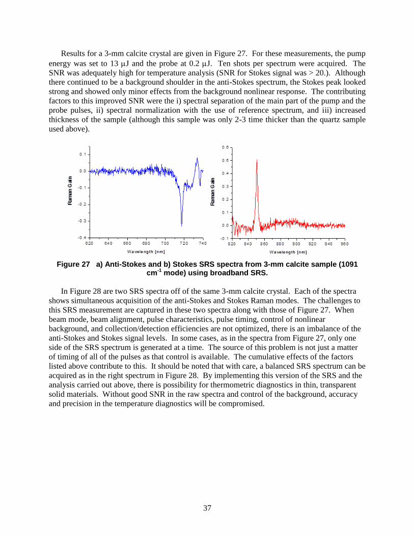
Results for a 3-mm calcite crystal are given in Figure 27. For these measurements, the pump

energy was set to 13 J and the probe at 0.2 J. Ten shots per spectrum were acquired. The

SNR was adequately high for temperature analysis (SNR for Stokes signal was > 20.). Although

there continued to be a background shoulder in the anti-Stokes spectrum, the Stokes peak looked

strong and showed only minor effects from the background nonlinear response. The contributing

factors to this improved SNR were the i) spectral separation of the main part of the pump and the

probe pulses, ii) spectral normalization with the use of reference spectrum, and iii) increased

thickness of the sample (although this sample was only 2-3 time thicker than the quartz sample

used above).

Figure 27 a) Anti-Stokes and b) Stokes SRS spectra from 3-mm calcite sample (1091 cm-1 mode) using broadband SRS.

In Figure 28 are two SRS spectra off of the same 3-mm calcite crystal. Each of the spectra

shows simultaneous acquisition of the anti-Stokes and Stokes Raman modes. The challenges to

this SRS measurement are captured in these two spectra along with those of Figure 27. When

beam mode, beam alignment, pulse characteristics, pulse timing, control of nonlinear

background, and collection/detection efficiencies are not optimized, there is an imbalance of the

anti-Stokes and Stokes signal levels. In some cases, as in the spectra from Figure 27, only one

side of the SRS spectrum is generated at a time. The source of this problem is not just a matter

of timing of all of the pulses as that control is available. The cumulative effects of the factors

listed above contribute to this. It should be noted that with care, a balanced SRS spectrum can be

acquired as in the right spectrum in Figure 28. By implementing this version of the SRS and the

analysis carried out above, there is possibility for thermometric diagnostics in thin, transparent

solid materials. Without good SNR in the raw spectra and control of the background, accuracy

and precision in the temperature diagnostics will be compromised.

38

Figure 28 SRS spectra from 3-mm calcite sample (1091 cm-1 mode) using broadband SRS.

As an added note, an optical heterodyne detection technique was carried out to try to increase

the SNR of the SRS signal. But the results showed that the rejection of the DC component of the

probe spectrum did not contribute to increased SNR. Better SNR was achieved with either the

direct subtraction of the pump-off probe spectrum or with the use of the reference pulse.

3.6 Conclusion The loss-to-gain ratio in femtosecond stimulated Raman scattering can be used for

temperature diagnostics in transparent, high quality solids. This method allows for access to

temperature on a picosecond time scale and does not require knowledge of material parameters.

Compared to spontaneous Raman scattering, the signal levels are orders of magnitude higher.

But significant care must be applied to generate precise anti-Stokes and Stokes SRS signals, and

samples with low SRS cross-sections require thicknesses beyond those of a thin film. Due to

pump induced effects such as nonlinearities and sample burning and low cross-section for SRS,

femtosecond SRS may have limited application for energetic materials if measurements require

thin samples and single-shot acquisition. But, for transparent, crystalline-like materials, SRS

could provide thermometric data for samples in the range of 100s of microns.

39

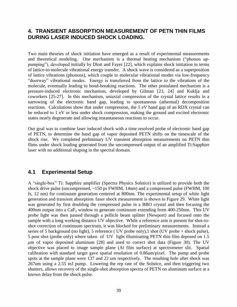
4. TRANSIENT ABSORPTION MEASUREMENT OF PETN THIN FILMS DURING LASER INDUCED SHOCK LOADING.

Two main theories of shock initiation have emerged as a result of experimental measurements

and theoretical modeling. One mechanism is a thermal heating mechanism (“phonon up-

pumping”), developed initially by Dlott and Fayer [22], which explains shock initiation in terms

of lattice-to-molecule vibrational energy transfer. A shock wave is considered as a superposition

of lattice vibrations (phonons), which couple to molecular vibrational modes via low-frequency

“doorway” vibrational modes. Energy is transferred from the lattice to the vibrations of the

molecule, eventually leading to bond-breaking reactions. The other postulated mechanism is a

pressure-induced electronic mechanism, developed by Gilman [23, 24] and Kuklja and

coworkers [25-27]. In this mechanism, uniaxial compression of the crystal lattice results in a

narrowing of the electronic band gap, leading to spontaneous (athermal) decomposition

reactions. Calculations show that under compression, the 5 eV band gap of an RDX crystal can

be reduced to 1 eV or less under shock compression, making the ground and excited electronic

states nearly degenerate and allowing instantaneous reactions to occur.

Our goal was to combine laser induced shock with a time resolved probe of electronic band gap

of PETN, to determine the band gap of vapor deposited PETN shifts on the timescale of the

shock rise. We completed preliminary UV transient absorption measurements on PETN thin

flims under shock loading generated from the uncompressed output of an amplified Ti:Sapphire

laser with no additional shaping in the spectral domain.

4.1 Experimental Setup

A “single-box” Ti: Sapphire amplifier (Spectra Physics Solstice) is utilized to provide both the

shock drive pulse (uncompressed, ~150 ps FWHM, 14nm) and a compressed pulse (FWHM, 100

fs, 12 nm) for continuum generation centered at 800nm. The experimental setup of white light

generation and transient absorption /laser shock measurement is shown in Figure 29. White light

was generated by first doubling the compressed pulse in a BBO crystal and then focusing the

400nm output into a CaF2 window to generate continuum extending from 400-250nm. This UV

probe light was then passed through a pellicle beam splitter (Newport) and focused onto the

sample with a long working distance UV objective. While a reference arm is present for shot-to-

shot correction of continuum spectrum, it was blocked for preliminary measurements. Instead a

series of 5 background (no light), 5 reference ( UV probe only),1 shot (UV probe + shock pulse),

5 post shot (probe only) where taken of UV light illuminating PETN thin film deposed on 1.5

m of vapor deposited aluminum [28] and used to correct shot data (Figure 30). The UV

objective was placed to image sample plane (Al film surface) at spectrometer slit. Spatial

calibration with standard target gave spatial resolution of 0.86um/pixel. The pump and probe

spots at the sample plane were 137 and 22 um respectively. The resulting hole after shock was

267um using a 2.55 mJ pump. Lowering the rep rate of the Solstice, and then triggering two

shutters, allows recovery of the single-shot absorption spectra of PETN on aluminum surface at a

known delay from the shock pulse.

40

The UV probe was imaged to the open slit of a 0.150-m imaging spectrometer with gratings

blazed at 300nm. A liquid nitrogen cooled CCD camera (Princeton UVSpec10) was directly

mated to the spectrometer to provide single-shot sensitivity out to 250 nm. Transient absorption

measurements were also carried out with the doubled amplifier pulse to compare to UV

continuum measurements using the same procedure (Figure 30).

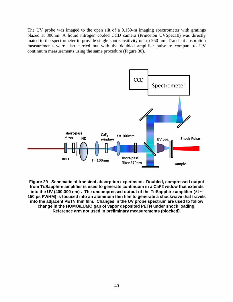
Figure 29 Schematic of transient absorption experiment. Doubled, compressed output from Ti:Sapphire amplifier is used to generate continuum in a CaF2 widow that extends

into the UV (400-300 nm) . The uncompressed output of the Ti:Sapphire amplifier (t ~ 150 ps FWHM) is focused into an aluminum thin film to generate a shockwave that travels

into the adjacent PETN thin film. Changes in the UV probe spectrum are used to follow change in the HOMO/LUMO gap of vapor deposited PETN under shock loading.

Reference arm not used in preliminary measurements (blocked).

41

Figure 30 Schematic of transient absorption experiment using only 400nm pump (no

continuum).

4.2 Results and Discussion

Results from shots on vapor deposited PETN thin films shown in Figure 31. Data were

recovered from 2D images of PETN thin films with the spectrometer centered at 300 nm. Data

taken for a series of delays referenced temporal overlap of pump and probe beams at sample

plane as measured by a photodiode with 1 ns time resolution. Data were integrated over vertical

dimension (260-320 pixels) in a region of high shock intensity, as determined from an image of

breakout post shock. Intensity variations were below or near reported absorbance attributed to

aluminum surface roughening in transient absorption measurements of unreactive shocked

liquids in contact with an aluminum ablator [29].

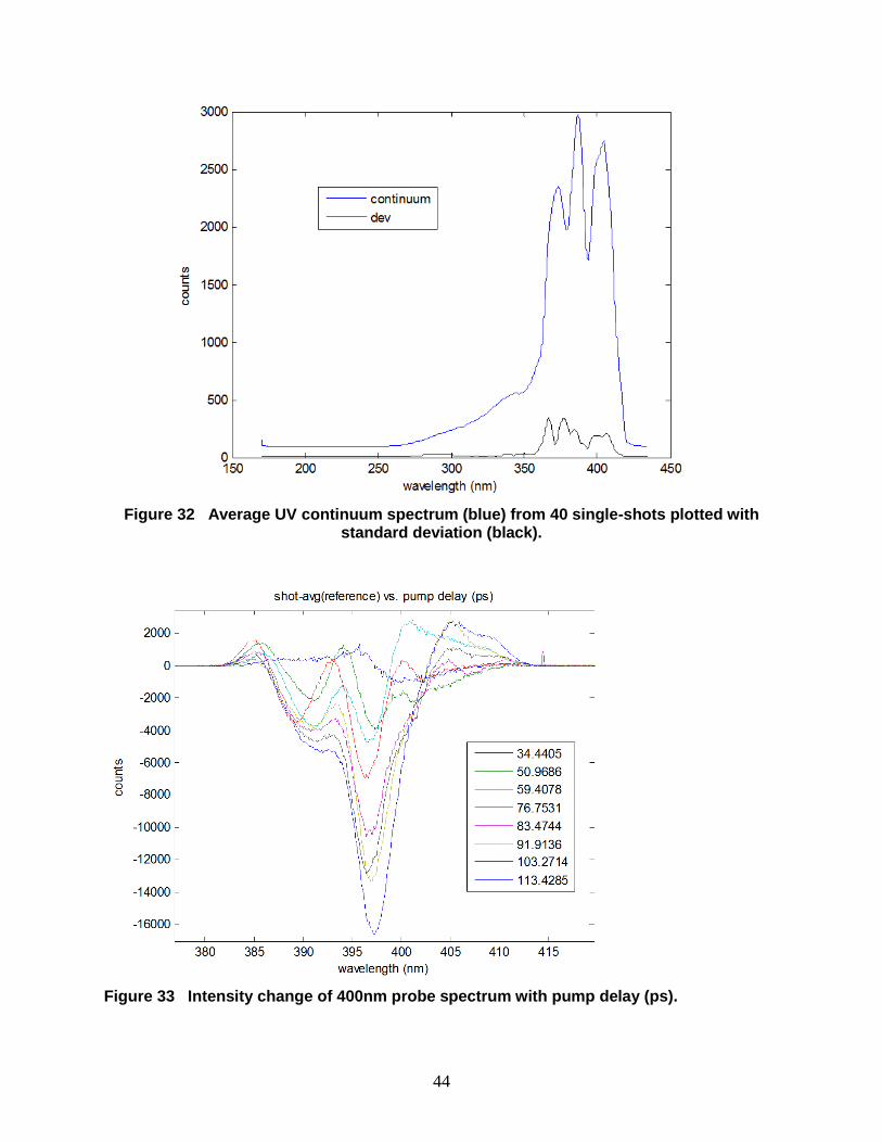
Since the shot-to-shot variation in the UV continuum is significant (Figure 31), the experiment

was repeated using only the 400-nm frequency-doubled laser pulse, with results shown in

Figures 32-35. In Figure 32, the probe spectrum in the vicinity of 400 nm is plotted alongside the

observed standard deviation in detector counts at each wavelength, revealing a more stable probe

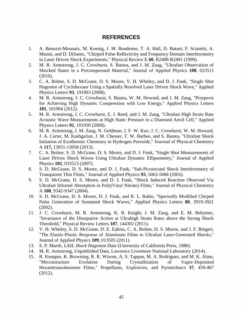
source than was observed with continuum generation. The change in the probe pulse spectrum

from the PETN sample during several single-shot laser drive measurements is shown in Figure

33. Each curve represents the change in the absorption probe for the indicate time delays

between the shock drive pulse and probe beam, revealing the evolution of the absorption

spectrum with time during laser drive. Larger intensity drops were observed as a function of time

delay (< 63% in some regions of the spectrum near 110-120 ps after the optical pump/probe

overlap delay in the absence of the sample).

42

43

Figure 31 2D and 1D images of continuum spectrum over a series of pump/probe delays. Reference and post spectra averaged over 5 spectra.

44

Figure 32 Average UV continuum spectrum (blue) from 40 single-shots plotted with

standard deviation (black).

Figure 33 Intensity change of 400nm probe spectrum with pump delay (ps).

45

REFERENCES

1. A. Benuzzi-Mounaix, M. Koenig, J. M. Boudenne, T. A. Hall, D. Batani, F. Scianitti, A.

Masini, and D. DiSanto, "Chirped Pulse Reflectivity and Frequency Domain Interferometry

in Laser Driven Shock Experiments," Physical Review E 60, R2488-R2491 (1999).

2. M. R. Armstrong, J. C. Crowhurst, S. Bastea, and J. M. Zaug, "Ultrafast Observation of

Shocked States in a Precompressed Material," Journal of Applied Physics 108, 023511

(2010).

3. C. A. Bolme, S. D. McGrane, D. S. Moore, V. H. Whitley, and D. J. Funk, "Single Shot

Hugoniot of Cyclohexane Using a Spatially Resolved Laser Driven Shock Wave," Applied

Physics Letters 93, 191903 (2008).

4. M. R. Armstrong, J. C. Crowhurst, S. Bastea, W. M. Howard, and J. M. Zaug, "Prospects

for Achieving High Dynamic Compression with Low Energy," Applied Physics Letters

101, 101904 (2012).

5. M. R. Armstrong, J. C. Crowhurst, E. J. Reed, and J. M. Zaug, "Ultrafast High Strain Rate

Acoustic Wave Measurements at High Static Pressure in a Diamond Anvil Cell," Applied

Physics Letters 92, 101930 (2008).

6. M. R. Armstrong, J. M. Zaug, N. Goldman, I. F. W. Kuo, J. C. Crowhurst, W. M. Howard,

J. A. Carter, M. Kashgarian, J. M. Chesser, T. W. Barbee, and S. Bastea, "Ultrafast Shock

Initiation of Exothermic Chemistry in Hydrogen Peroxide," Jourrnal of Physical Chemistry

A 117, 13051-13058 (2013).

7. C. A. Bolme, S. D. McGrane, D. S. Moore, and D. J. Funk, "Single Shot Measurements of

Laser Driven Shock Waves Using Ultrafast Dynamic Ellipsometry," Journal of Applied

Physics 102, 033513 (2007).

8. S. D. McGrane, D. S. Moore, and D. J. Funk, "Sub-Picosecond Shock Interferometry of

Transparent Thin Films," Journal of Applied Physics 93, 5063-5068 (2003).

9. S. D. McGrane, D. S. Moore, and D. J. Funk, "Shock Induced Reaction Observed Via

Ultrafast Infrared Absorption in Poly(Vinyl Nitrate) Films," Journal of Physical Chemistry

A 108, 9342-9347 (2004).

10. S. D. McGrane, D. S. Moore, D. J. Funk, and R. L. Rabie, "Spectrally Modified Chirped

Pulse Generation of Sustained Shock Waves," Applied Physics Letters 80, 3919-3921

(2002).

11. J. C. Crowhurst, M. R. Armstrong, K. B. Knight, J. M. Zaug, and E. M. Behymer,

"Invariance of the Dissipative Action at Ultrahigh Strain Rates above the Strong Shock

Threshold," Physical Review Letters 107, 144302 (2011).

12. V. H. Whitley, S. D. McGrane, D. E. Eakins, C. A. Bolme, D. S. Moore, and J. F. Bingert,

"The Elastic-Plastic Response of Aluminum Films to Ultrafast Laser-Generated Shocks,"

Journal of Applied Physics 109, 013505 (2011).

13. S. P. Marsh, LASL Shock Hugoniot Data (University of California Press, 1980).

14. M. R. Armstrong, Unpublished Data, Lawrence Livermore National Laboratory (2014).

15. R. Knepper, K. Browning, R. R. Wixom, A. S. Tappan, M. A. Rodriguez, and M. K. Alam,

"Microstructure Evolution During Crystallization of Vapor-Deposited

Hexanitroazobenzene Films," Propellants, Explosives, and Pyrotechnics 37, 459-467

(2012).

46

16. W. C. McCrone, "Crystallographic Study of Hexanitroazobenzene (HNAB)", SAND75-

7067, Sandia National Laboratories (1975).

17. E. J. Graeber, and B. Morosin, "The Crystal Structures of 2,2’,4,4’,6,6’-

Hexanitroazobenzene (HNAB), Forms I and Ii," Acta Crystallographica B30, 310-317

(1974).

18. S. Roy, J. R. Gord, and A. K. Patnaik, "Recent Advances in Coherent Anti-Stokes Raman

Scattering Spectroscopy: Fundamental Developments and Applications in Reacting Flows,"

Progress in Energy and Combustion Science 36, 280-306 (2010).

19. N. C. Dang, C. A. Bolme, D. S. Moore, and S. D. McGrane, "Femtosecond Stimulated

Raman Scattering Picosecond Molecular Thermometry in Condensed Phases," Physical

Review Letters 107, 043001 (2011).

20. N. C. Dang, C. A. Bolme, D. S. Moore, and S. D. McGrane, "Temperature Measurements

in Condensed Phases Using Non-Resonant Femtosecond Stimulated Raman Scattering,"

Journal of Raman Spectrscopy 44, 433-439 (2012).

21. S. M. Shapiro, D. C. O'Shea, and H. Z. Cummins, "Raman Scattering Study of the Aplpha-

Beta Phase Transition in Quartz," Physical Review Letters 19, 361-364 (1967).

22. D. D. Dlott, and M. D. Fayer, "Vibrational up Pumping, Defect Hot Spot Formation, and

the Onset of Chemistry," Journal of Chemical Physics 92, 3798-3812 (1990).

23. J. J. Gilman, "Chemical Reactions at Detonation Fronts," Philosophical Magazine B 71,

1057-1068 (1995).

24. J. J. Gilman, "Mechanochemistry," Science 274, 5284 (1996).

25. M. M. Kuklja, "Role of Electronic Excitations in Explosive Decomposition of Solids,"

Journal of Applied Physics 89, 4156-4166 (2001).

26. M. M. Kuklja, "On the Initiation of Chemical Reactions by Electronic Excitations in

Molecular Solids," Applied Physics A 76, 359-366 (2003).

27. M. M. Kuklja, E. V. Stefanovich, and A. B. Kunz, "An Excitonic Mechanism of

Detonation Initiation in Explosives," Journal of Chemical Physics 112, 3417-3423 (2000).

28. R. Knepper, "Controlling the Microstructure of Vapor-Deposited Pentaerythritol," Journal

of Materials Research 26, 1605-1613 (2011).

29. N. C. Dang, C. A. Bolme, D. S. Moore, and S. D. McGrane, "Shock Induced Chemistry in

Liquids Studied with Ultrafast Dynamic Ellipsometry and Visible Transient Absorption

Spectroscopy," Journal of Physical Chemistry A 116, 10301-10309 (2012).

47

DISTRIBUTION (sent electronically)

1 MS1454 D.A. Farrow 02554

1 MS1454 B.A. Jilek 02554

1 MS1454 R. Knepper 02554

1 MS1454 I.T. Kohl 02554

1 MS1454 L.M.G. Minier 02554

1 MS1454 A.S. Tappan 02554

1 MS1454 W.M. Trott 02554

1 MS1454 R.R. Wixom 02554

1 MS1453 J.L. Moya 02550

1 MS1190 C.J. Bourdon 01675

1 MS1153 J. Urayama 05444

1 MS0828 T.L. Durbin 01512

1 MS0826 S.P. Kearney 01512

1 MS0359 D.L. Chavez, LDRD Office 07911

1 MS0899 Technical Library 09536 (electronic copy)