ultralarge)mul,ple)sequence)alignment - university...
TRANSCRIPT

Ultra-‐large Mul,ple Sequence Alignment
Tandy Warnow Founder Professor of Engineering
The University of Illinois at Urbana-‐Champaign hEp://tandy.cs.illinois.edu
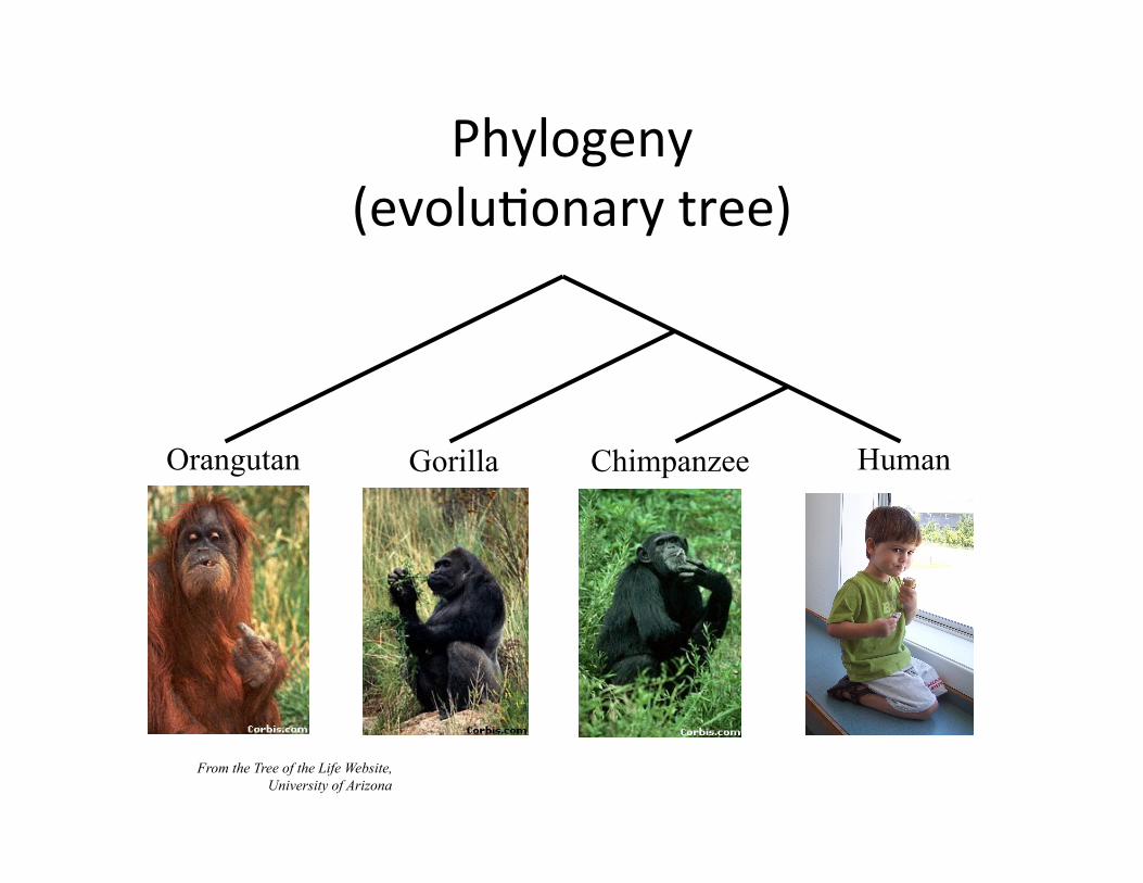
Orangutan Gorilla Chimpanzee Human
From the Tree of the Life Website, University of Arizona
Phylogeny (evolu,onary tree)
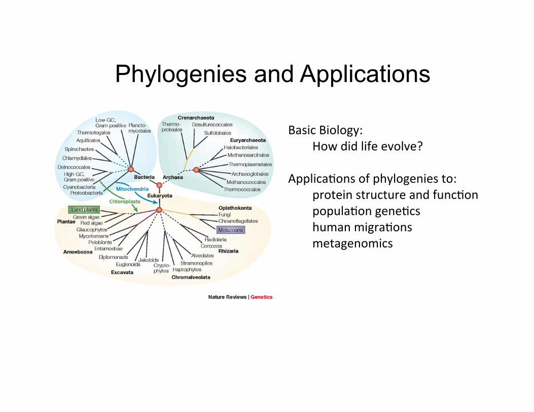
Phylogenies and Applications
Basic Biology: How did life evolve?
Applica,ons of phylogenies to: protein structure and func,on popula,on gene,cs human migra,ons metagenomics

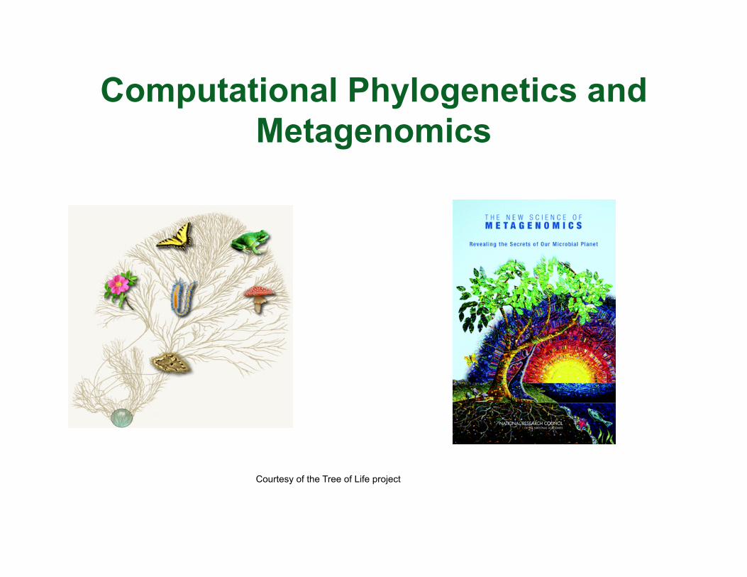
Computational Phylogenetics and Metagenomics
Courtesy of the Tree of Life project
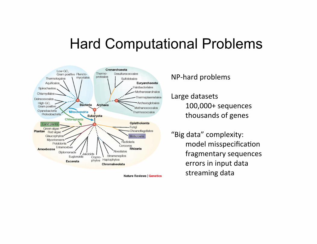
Hard Computational Problems
NP-‐hard problems Large datasets
100,000+ sequences thousands of genes
“Big data” complexity:
model misspecifica,on fragmentary sequences errors in input data streaming data
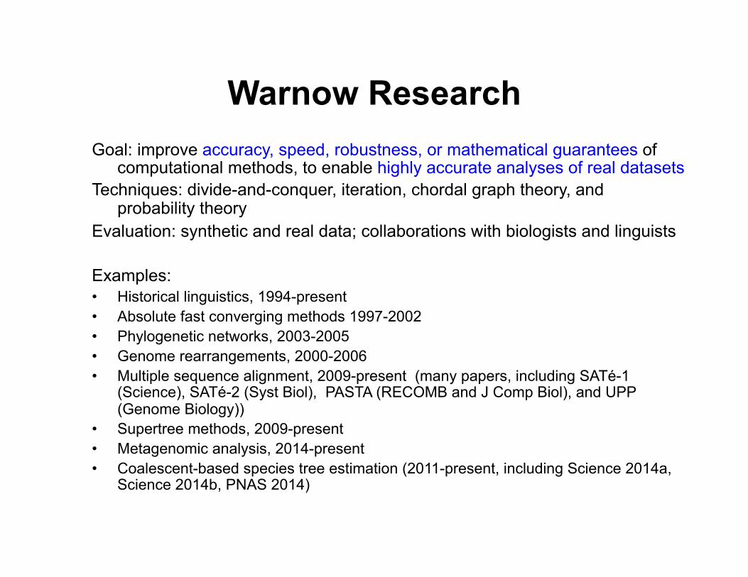
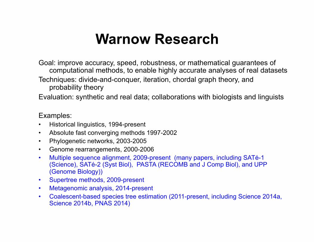
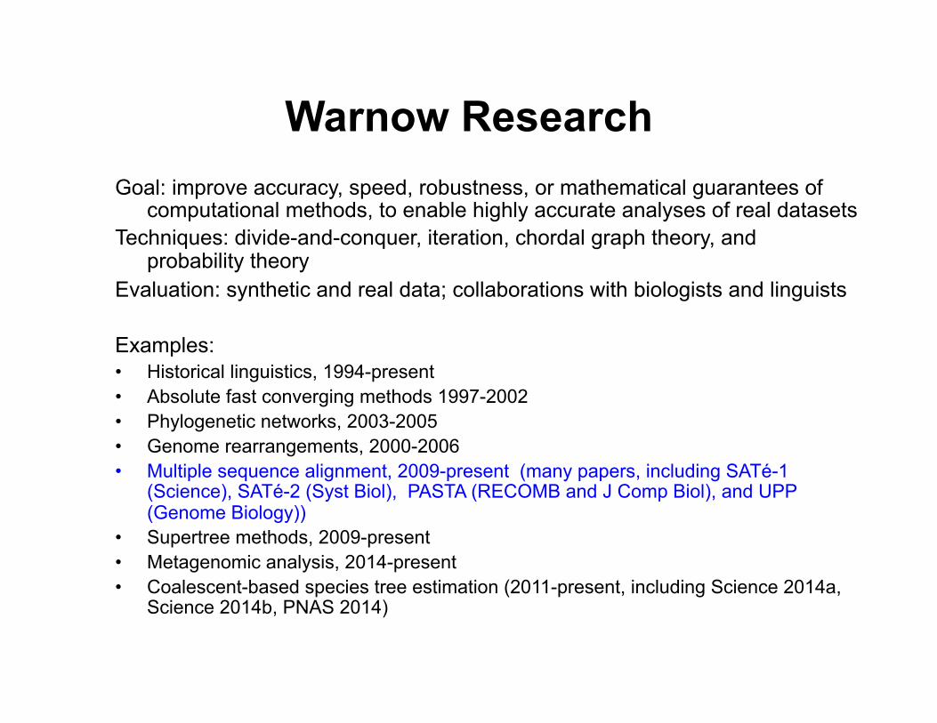
Warnow Research Goal: improve accuracy, speed, robustness, or mathematical guarantees of
computational methods, to enable highly accurate analyses of real datasets Techniques: divide-and-conquer, iteration, chordal graph theory, and
probability theory Evaluation: synthetic and real data; collaborations with biologists and linguists Examples: • Historical linguistics, 1994-present • Absolute fast converging methods 1997-2002 • Phylogenetic networks, 2003-2005 • Genome rearrangements, 2000-2006 • Multiple sequence alignment, 2009-present (many papers, including SATé-1
(Science), SATé-2 (Syst Biol), PASTA (RECOMB and J Comp Biol), and UPP (Genome Biology))
• Supertree methods, 2009-present • Metagenomic analysis, 2014-present • Coalescent-based species tree estimation (2011-present, including Science 2014a,
Science 2014b, PNAS 2014)
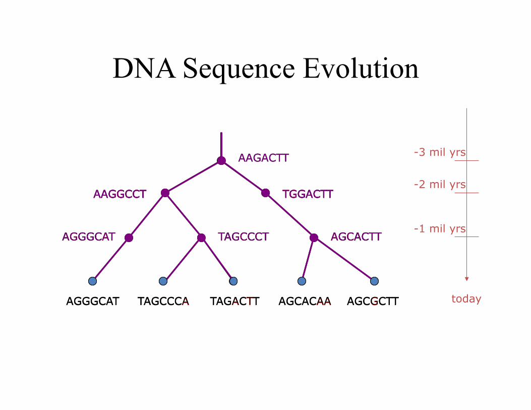
DNA Sequence Evolution
AAGACTT
TGGACTT AAGGCCT
-3 mil yrs
-2 mil yrs
-1 mil yrs
today
AGGGCAT TAGCCCT AGCACTT
AAGGCCT TGGACTT
TAGCCCA TAGACTT AGCGCTT AGCACAA AGGGCAT
AGGGCAT TAGCCCT AGCACTT
AAGACTT
TGGACTT AAGGCCT
AGGGCAT TAGCCCT AGCACTT
AAGGCCT TGGACTT
AGCGCTT AGCACAA TAGACTT TAGCCCA AGGGCAT
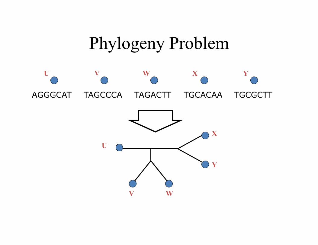
Phylogeny Problem
TAGCCCA TAGACTT TGCACAA TGCGCTT AGGGCAT
U V W X Y
U
V W
X
Y
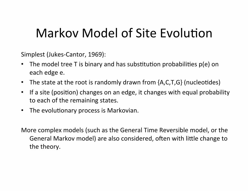
Markov Model of Site Evolu,on Simplest (Jukes-‐Cantor, 1969): • The model tree T is binary and has subs,tu,on probabili,es p(e) on
each edge e. • The state at the root is randomly drawn from {A,C,T,G} (nucleo,des) • If a site (posi,on) changes on an edge, it changes with equal probability
to each of the remaining states. • The evolu,onary process is Markovian.
More complex models (such as the General Time Reversible model, or the General Markov model) are also considered, o`en with liEle change to the theory.
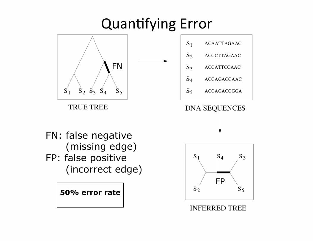
Quan,fying Error
FN: false negative (missing edge) FP: false positive (incorrect edge)
FN
FP 50% error rate
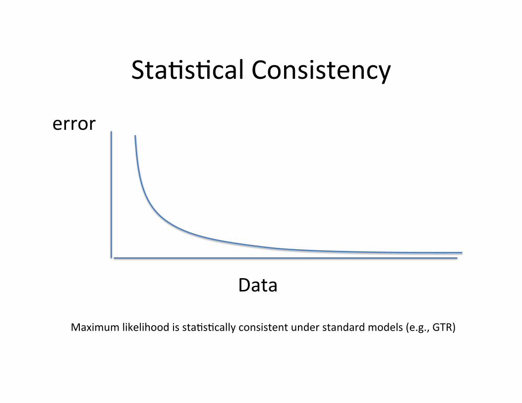
Sta,s,cal Consistency
error
Data
Maximum likelihood is sta,s,cally consistent under standard models (e.g., GTR)
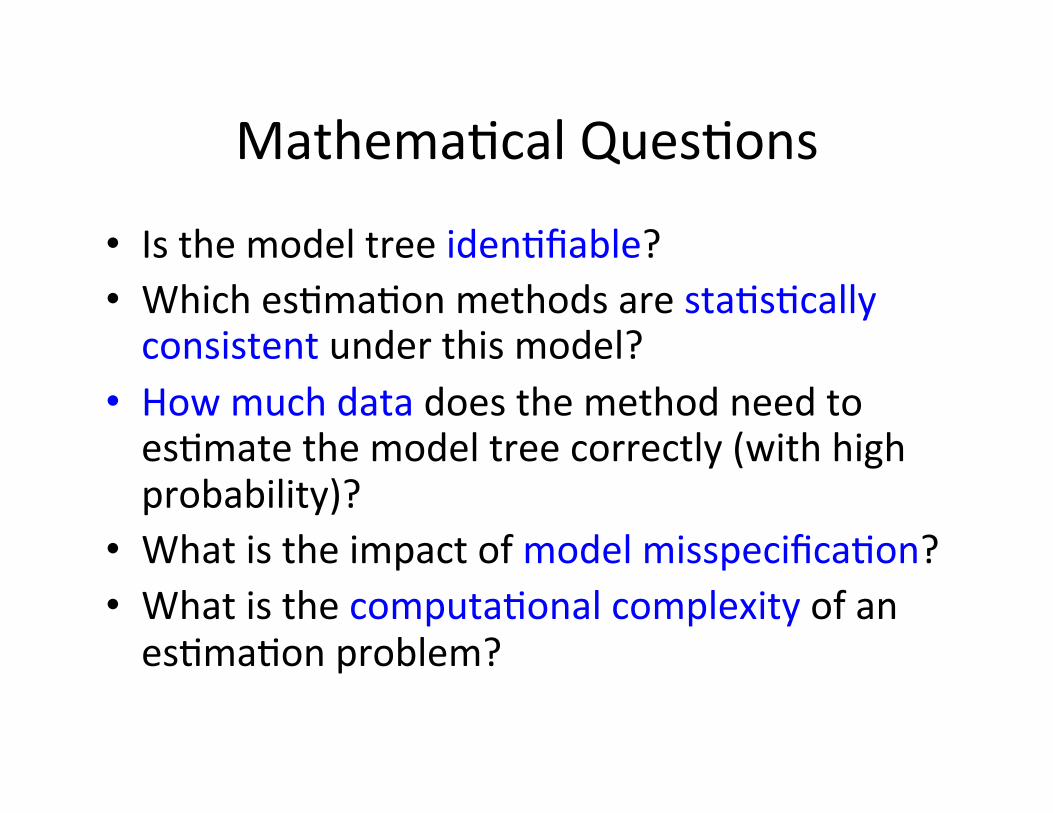
Mathema,cal Ques,ons
• Is the model tree iden,fiable? • Which es,ma,on methods are sta,s,cally consistent under this model?
• How much data does the method need to es,mate the model tree correctly (with high probability)?
• What is the impact of model misspecifica,on? • What is the computa,onal complexity of an es,ma,on problem?
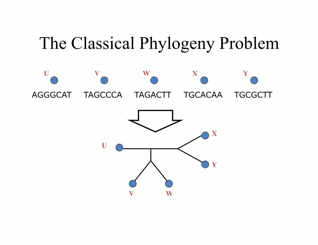
The Classical Phylogeny Problem
TAGCCCA TAGACTT TGCACAA TGCGCTT AGGGCAT
U V W X Y
U
V W
X
Y
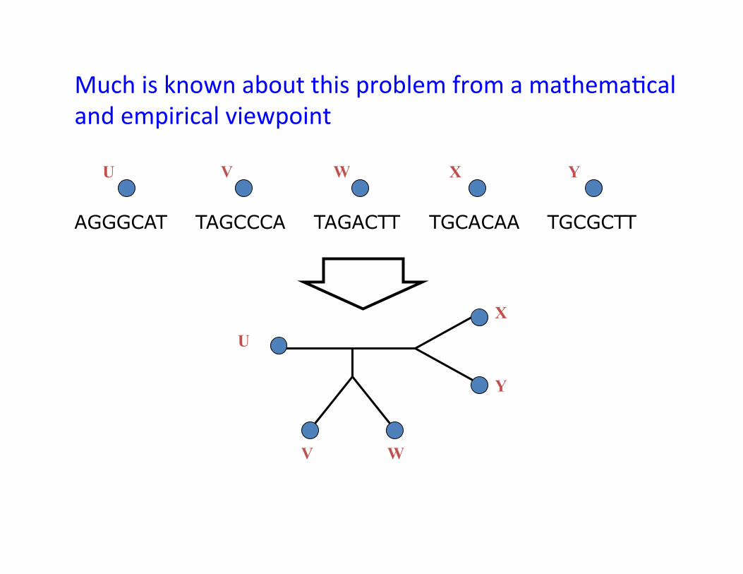
TAGCCCA TAGACTT TGCACAA TGCGCTT AGGGCAT
U V W X Y
U
V W
X
Y
Much is known about this problem from a mathema,cal and empirical viewpoint
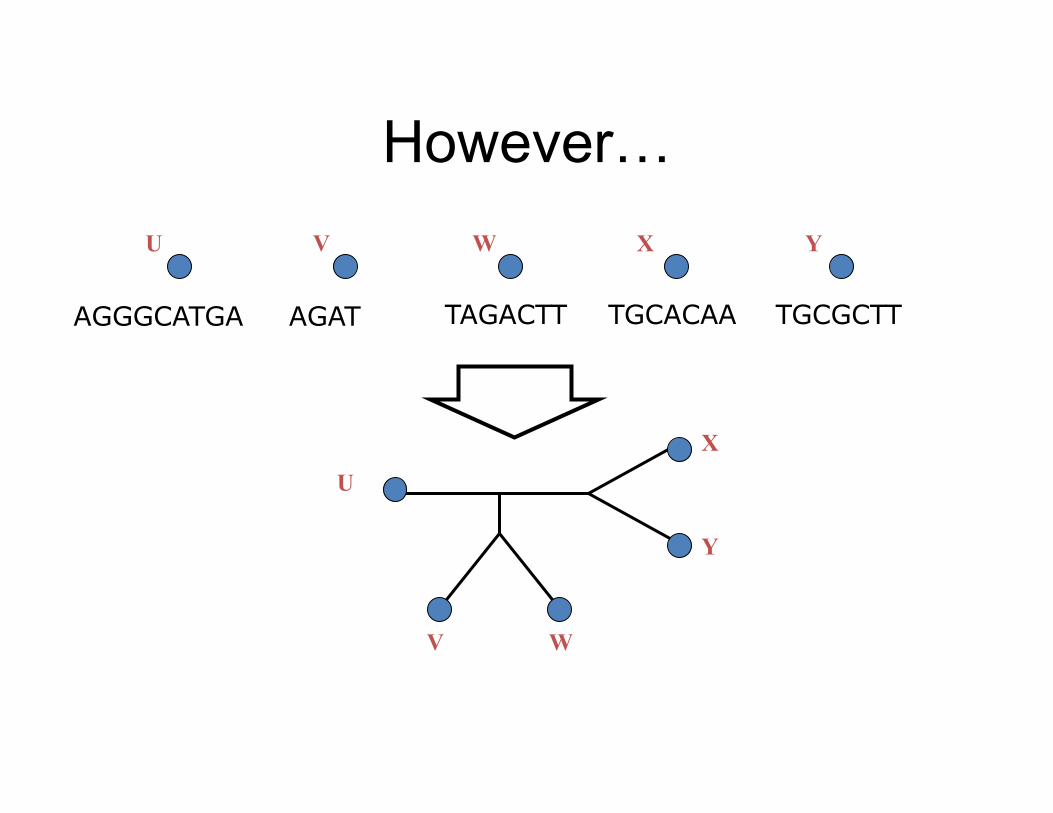
AGAT TAGACTT TGCACAA TGCGCTT AGGGCATGA
U V W X Y
U
V W
X
Y
However…
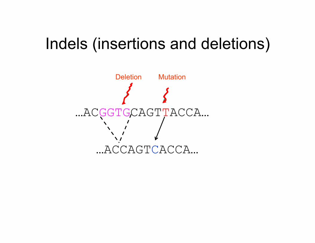
…ACGGTGCAGTTACCA…
Mutation Deletion
…ACCAGTCACCA…
Indels (insertions and deletions)
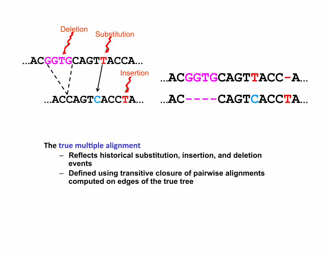
…ACGGTGCAGTTACC-A…
…AC----CAGTCACCTA…
The true mul*ple alignment – Reflects historical substitution, insertion, and deletion
events – Defined using transitive closure of pairwise alignments
computed on edges of the true tree
…ACGGTGCAGTTACCA…
Substitution Deletion
…ACCAGTCACCTA…
Insertion
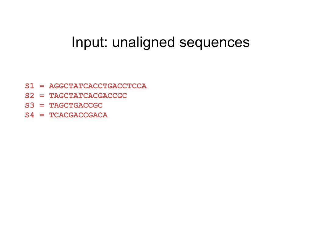
Input: unaligned sequences
S1 = AGGCTATCACCTGACCTCCA S2 = TAGCTATCACGACCGC S3 = TAGCTGACCGC S4 = TCACGACCGACA
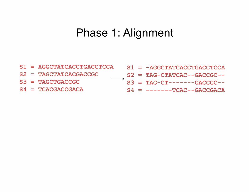
Phase 1: Alignment
S1 = -AGGCTATCACCTGACCTCCA S2 = TAG-CTATCAC--GACCGC-- S3 = TAG-CT-------GACCGC-- S4 = -------TCAC--GACCGACA
S1 = AGGCTATCACCTGACCTCCA S2 = TAGCTATCACGACCGC S3 = TAGCTGACCGC S4 = TCACGACCGACA
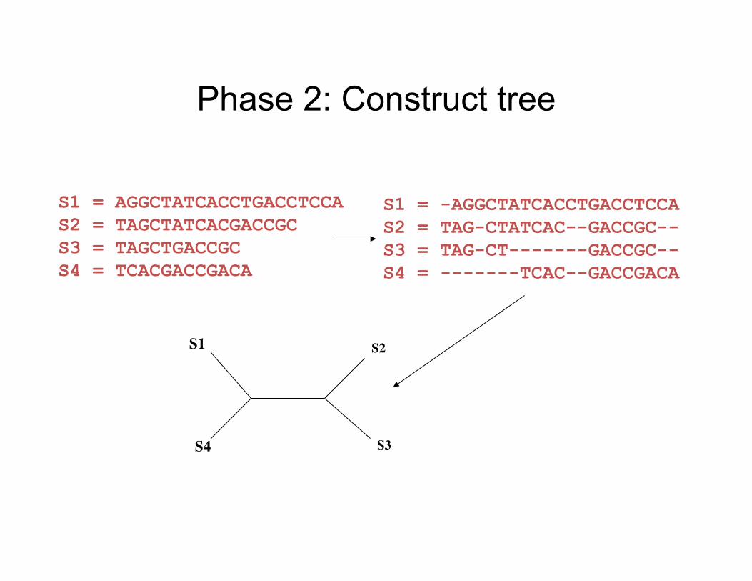
Phase 2: Construct tree
S1 = -AGGCTATCACCTGACCTCCA S2 = TAG-CTATCAC--GACCGC-- S3 = TAG-CT-------GACCGC-- S4 = -------TCAC--GACCGACA
S1 = AGGCTATCACCTGACCTCCA S2 = TAGCTATCACGACCGC S3 = TAGCTGACCGC S4 = TCACGACCGACA
S1
S4
S2
S3
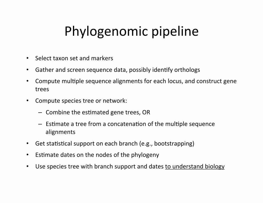
Phylogenomic pipeline
• Select taxon set and markers
• Gather and screen sequence data, possibly iden,fy orthologs
• Compute mul,ple sequence alignments for each locus, and construct gene trees
• Compute species tree or network:
– Combine the es,mated gene trees, OR
– Es,mate a tree from a concatena,on of the mul,ple sequence alignments
• Get sta,s,cal support on each branch (e.g., bootstrapping)
• Es,mate dates on the nodes of the phylogeny
• Use species tree with branch support and dates to understand biology
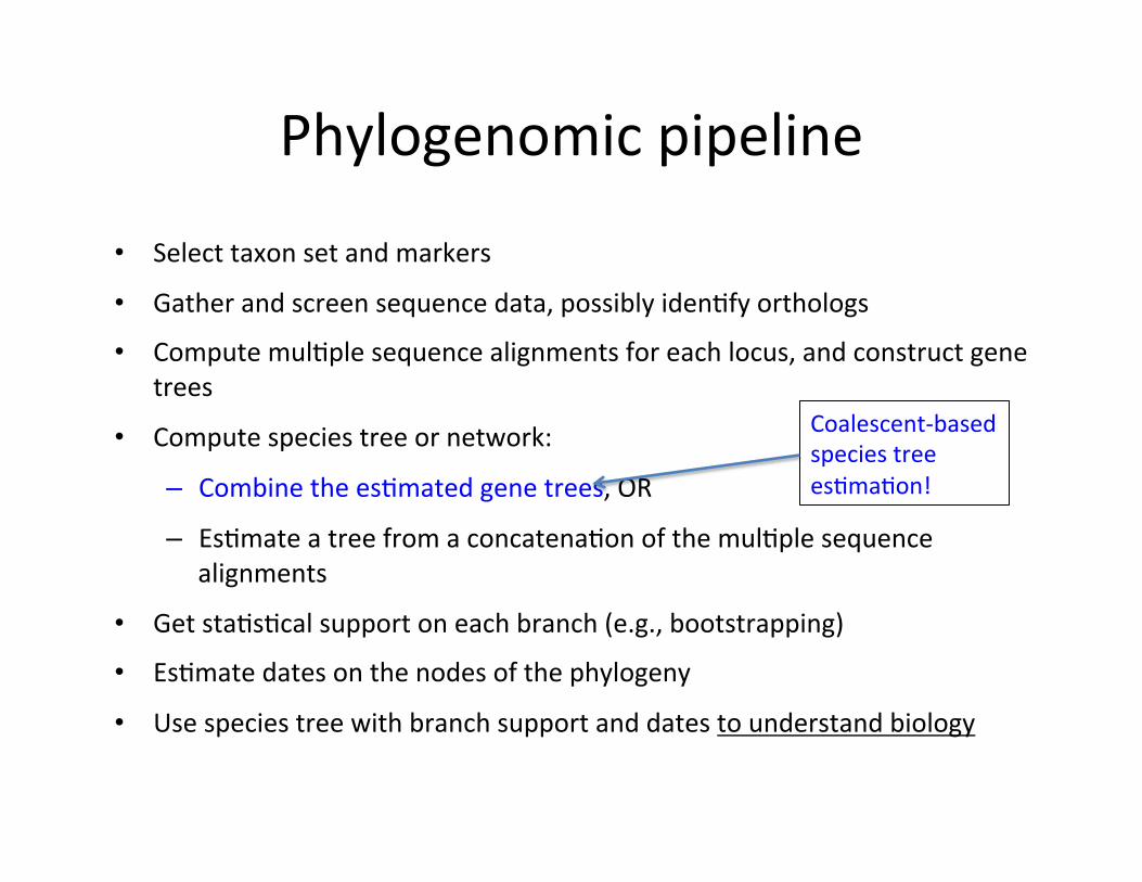
Coalescent-‐based species tree es,ma,on!
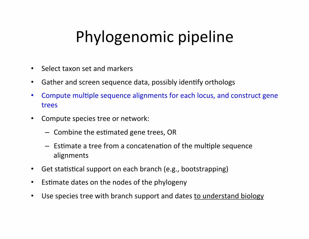
Phylogenomic pipeline
• Select taxon set and markers
• Gather and screen sequence data, possibly iden,fy orthologs
• Compute mul,ple sequence alignments for each locus, and construct gene trees
• Compute species tree or network:
– Combine the es,mated gene trees, OR
– Es,mate a tree from a concatena,on of the mul,ple sequence alignments
• Get sta,s,cal support on each branch (e.g., bootstrapping)
• Es,mate dates on the nodes of the phylogeny
• Use species tree with branch support and dates to understand biology
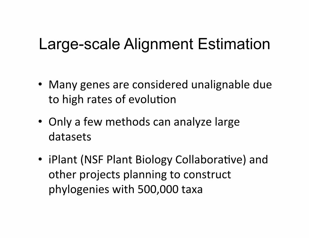
Large-scale Alignment Estimation
• Many genes are considered unalignable due to high rates of evolu,on
• Only a few methods can analyze large datasets
• iPlant (NSF Plant Biology Collabora,ve) and other projects planning to construct phylogenies with 500,000 taxa
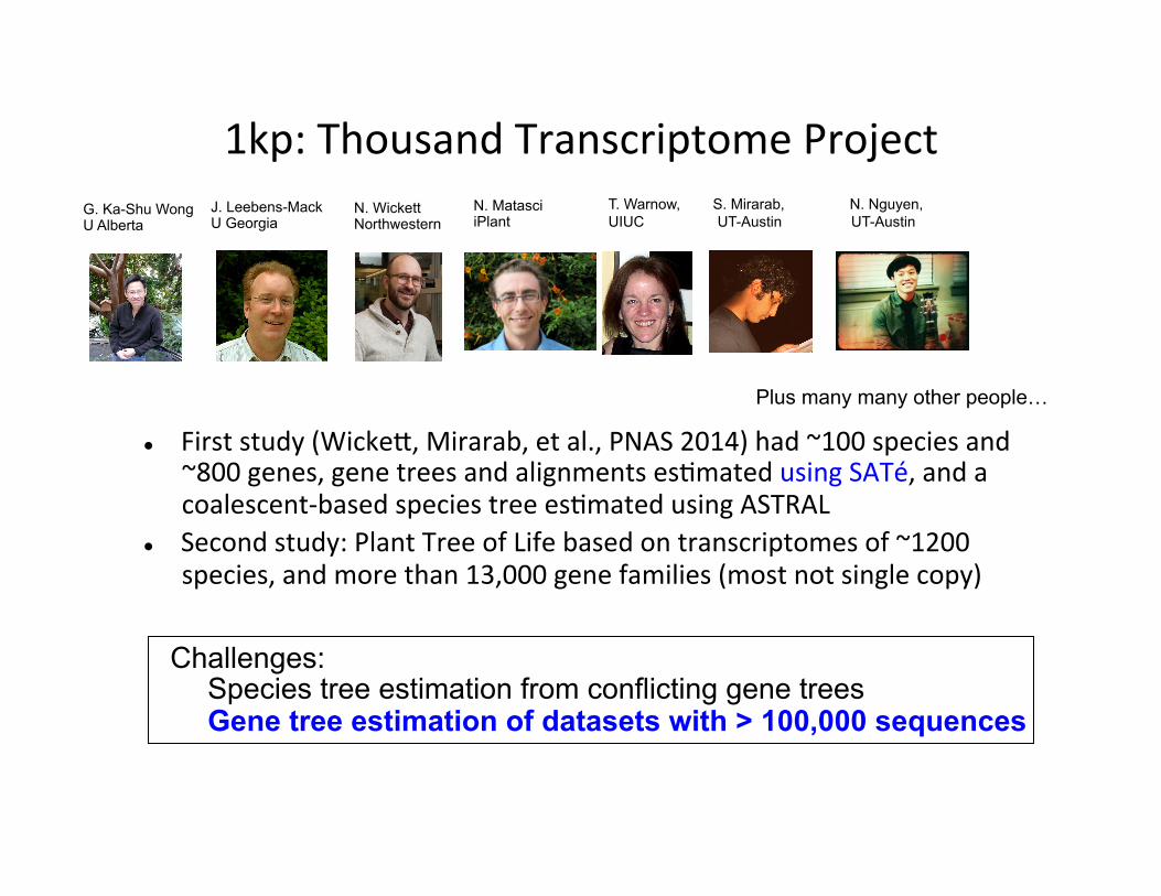
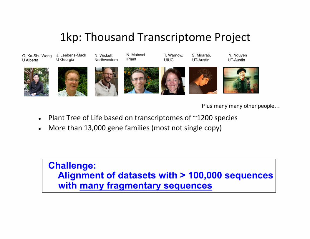
1kp: Thousand Transcriptome Project
l First study (WickeE, Mirarab, et al., PNAS 2014) had ~100 species and ~800 genes, gene trees and alignments es,mated using SATé, and a coalescent-‐based species tree es,mated using ASTRAL
l Second study: Plant Tree of Life based on transcriptomes of ~1200 species, and more than 13,000 gene families (most not single copy)
Gene Tree Incongruence
G. Ka-Shu Wong U Alberta
N. Wickett Northwestern
J. Leebens-Mack U Georgia
N. Matasci iPlant
T. Warnow, S. Mirarab, N. Nguyen, UIUC UT-Austin UT-Austin
Challenges: Species tree estimation from conflicting gene trees Gene tree estimation of datasets with > 100,000 sequences
Plus many many other people…
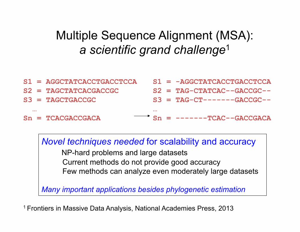
Multiple Sequence Alignment (MSA): a scientific grand challenge1
S1 = -AGGCTATCACCTGACCTCCA S2 = TAG-CTATCAC--GACCGC-- S3 = TAG-CT-------GACCGC-- … Sn = -------TCAC--GACCGACA
S1 = AGGCTATCACCTGACCTCCA S2 = TAGCTATCACGACCGC S3 = TAGCTGACCGC … Sn = TCACGACCGACA
Novel techniques needed for scalability and accuracy NP-hard problems and large datasets Current methods do not provide good accuracy Few methods can analyze even moderately large datasets Many important applications besides phylogenetic estimation
1 Frontiers in Massive Data Analysis, National Academies Press, 2013
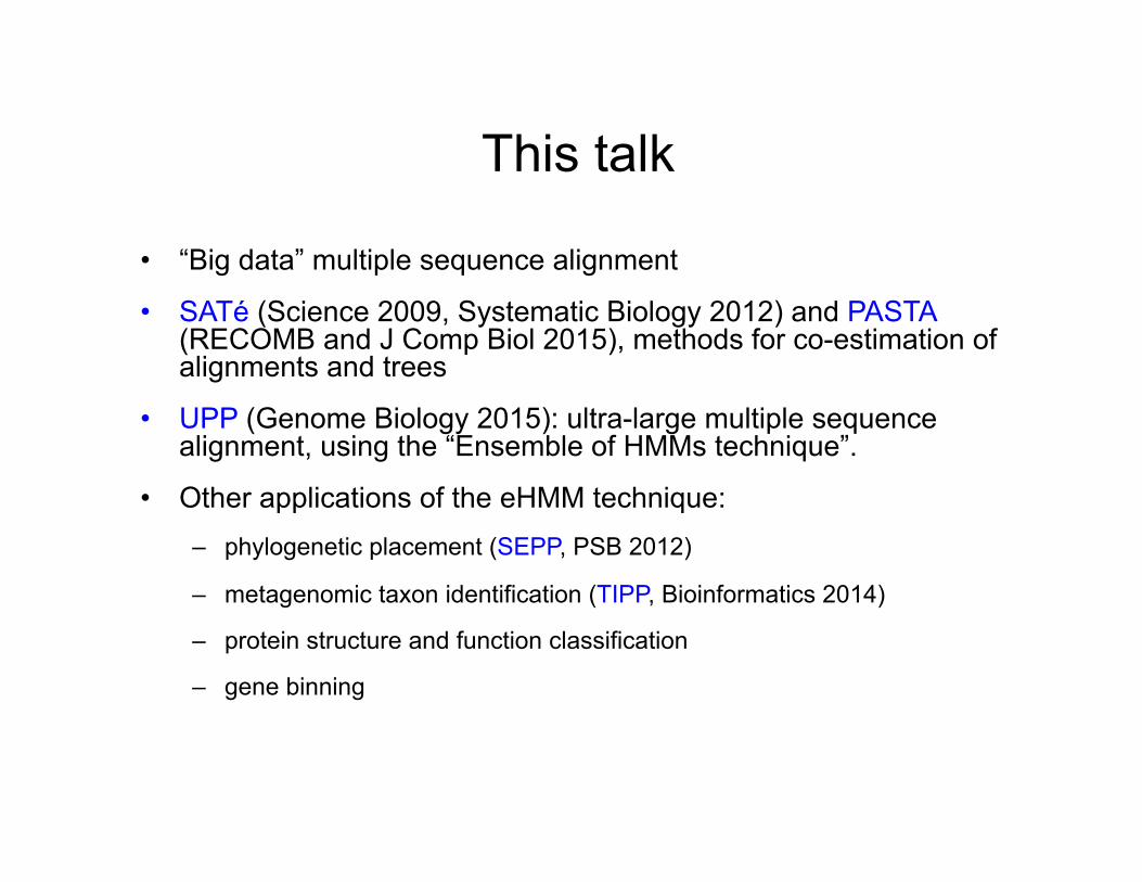
This talk
• “Big data” multiple sequence alignment
• SATé (Science 2009, Systematic Biology 2012) and PASTA (RECOMB and J Comp Biol 2015), methods for co-estimation of alignments and trees
• UPP (Genome Biology 2015): ultra-large multiple sequence alignment, using the “Ensemble of HMMs technique”.
• Other applications of the eHMM technique: – phylogenetic placement (SEPP, PSB 2012)
– metagenomic taxon identification (TIPP, Bioinformatics 2014)
– protein structure and function classification
– gene binning

Mul,ple Sequence Alignment
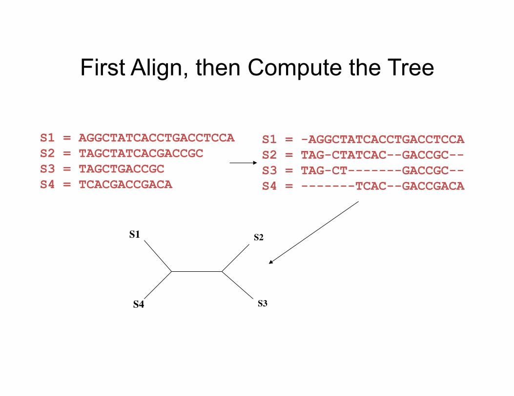
First Align, then Compute the Tree
S1 = -AGGCTATCACCTGACCTCCA S2 = TAG-CTATCAC--GACCGC-- S3 = TAG-CT-------GACCGC-- S4 = -------TCAC--GACCGACA
S1 = AGGCTATCACCTGACCTCCA S2 = TAGCTATCACGACCGC S3 = TAGCTGACCGC S4 = TCACGACCGACA
S1
S4
S2
S3

S1 = -AGGCTATCACCTGACCTCCA S2 = TAG-CTATCAC--GACCGC-- S3 = TAG-CT-------GACCGC-- S4 = -------TCAC--GACCGACA
S1 = AGGCTATCACCTGACCTCCA S2 = TAGCTATCACGACCGC S3 = TAGCTGACCGC S4 = TCACGACCGACA
S1
S4
S2
S3
Co-‐es,ma,on would be much beEer!!!
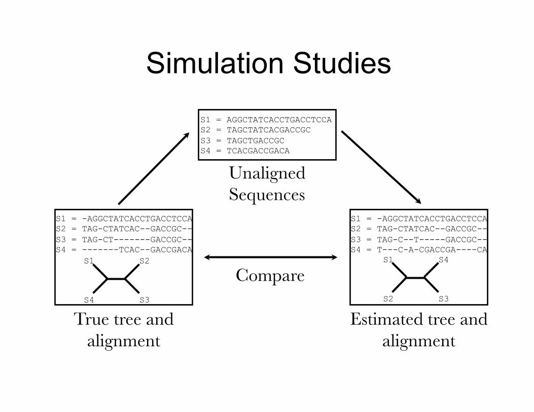
Simulation Studies
S1 S2
S3 S4
S1 = -AGGCTATCACCTGACCTCCA S2 = TAG-CTATCAC--GACCGC-- S3 = TAG-CT-------GACCGC-- S4 = -------TCAC--GACCGACA
S1 = AGGCTATCACCTGACCTCCA S2 = TAGCTATCACGACCGC S3 = TAGCTGACCGC S4 = TCACGACCGACA
S1 = -AGGCTATCACCTGACCTCCA S2 = TAG-CTATCAC--GACCGC-- S3 = TAG-C--T-----GACCGC-- S4 = T---C-A-CGACCGA----CA
Compare
True tree and alignment
S1 S4
S3 S2
Estimated tree and alignment
Unaligned Sequences
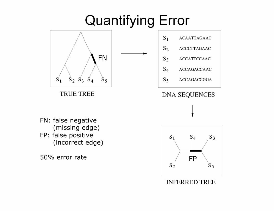
Quantifying Error
FN: false negative (missing edge) FP: false positive (incorrect edge) 50% error rate
FN
FP
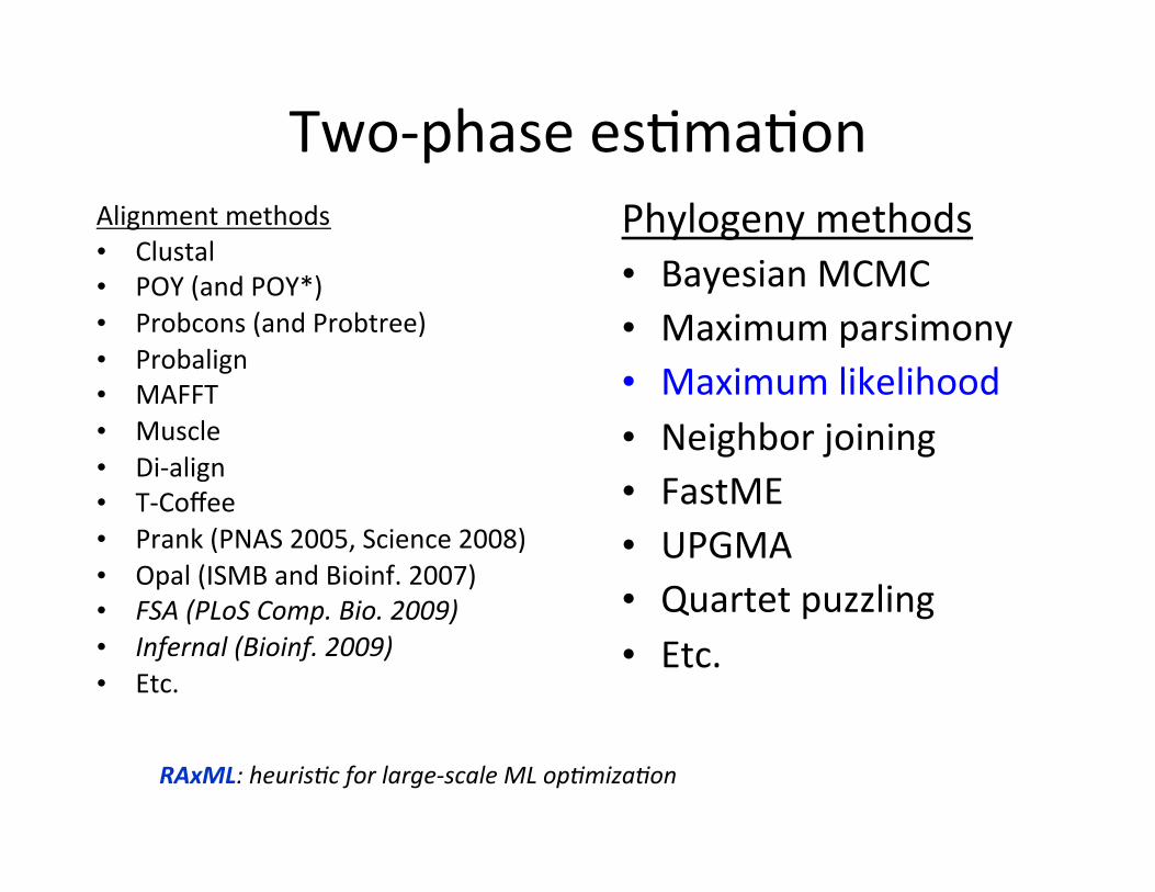
Two-‐phase es,ma,on Alignment methods • Clustal • POY (and POY*) • Probcons (and Probtree) • Probalign • MAFFT • Muscle • Di-‐align • T-‐Coffee • Prank (PNAS 2005, Science 2008) • Opal (ISMB and Bioinf. 2007) • FSA (PLoS Comp. Bio. 2009) • Infernal (Bioinf. 2009) • Etc.
Phylogeny methods • Bayesian MCMC • Maximum parsimony • Maximum likelihood • Neighbor joining • FastME • UPGMA • Quartet puzzling • Etc.
RAxML: heuris>c for large-‐scale ML op>miza>on
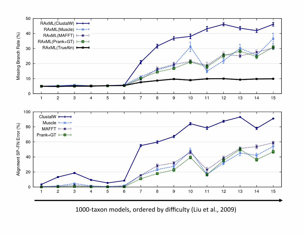
1000-‐taxon models, ordered by difficulty (Liu et al., 2009)
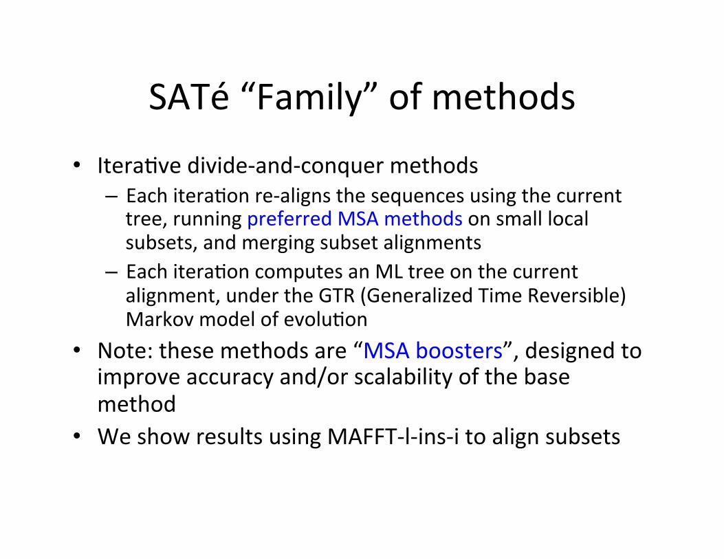
SATé “Family” of methods
• Itera,ve divide-‐and-‐conquer methods – Each itera,on re-‐aligns the sequences using the current tree, running preferred MSA methods on small local subsets, and merging subset alignments
– Each itera,on computes an ML tree on the current alignment, under the GTR (Generalized Time Reversible) Markov model of evolu,on
• Note: these methods are “MSA boosters”, designed to improve accuracy and/or scalability of the base method
• We show results using MAFFT-‐l-‐ins-‐i to align subsets

Re-aligning on a tree A
B D
C
Merge sub-alignments
Estimate ML tree on merged
alignment
Decompose dataset
A B
C D
Align subsets
A B
C D
ABCD
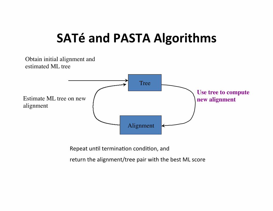
SATé and PASTA Algorithms
Estimate ML tree on new alignment
Tree
Obtain initial alignment and estimated ML tree
Use tree to compute new alignment
Alignment
Repeat un,l termina,on condi,on, and
return the alignment/tree pair with the best ML score
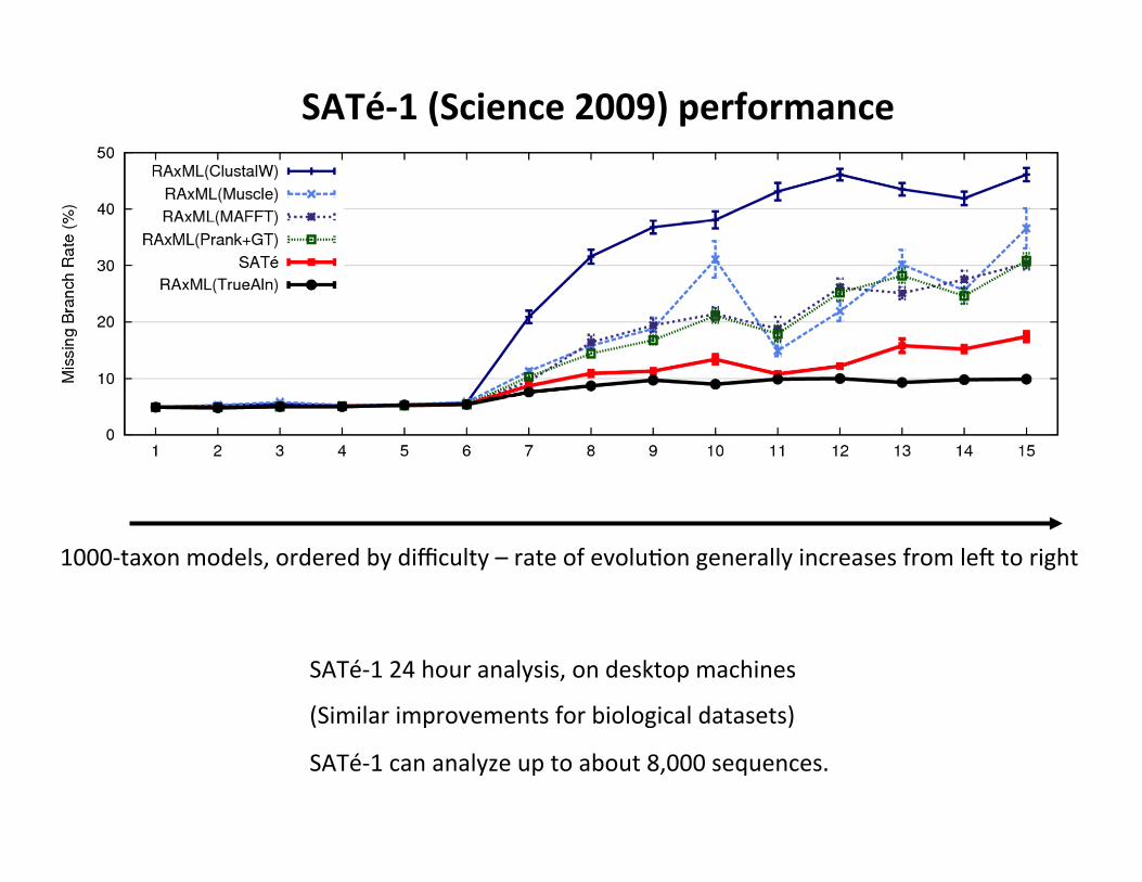
1000-‐taxon models, ordered by difficulty – rate of evolu,on generally increases from le` to right
SATé-‐1 24 hour analysis, on desktop machines
(Similar improvements for biological datasets)
SATé-‐1 can analyze up to about 8,000 sequences.
SATé-‐1 (Science 2009) performance

1000-‐taxon models ranked by difficulty
SATé-‐1 and SATé-‐2 (Systema*c Biology, 2012)
SATé-‐1: up to 8K SATé-‐2: up to ~50K
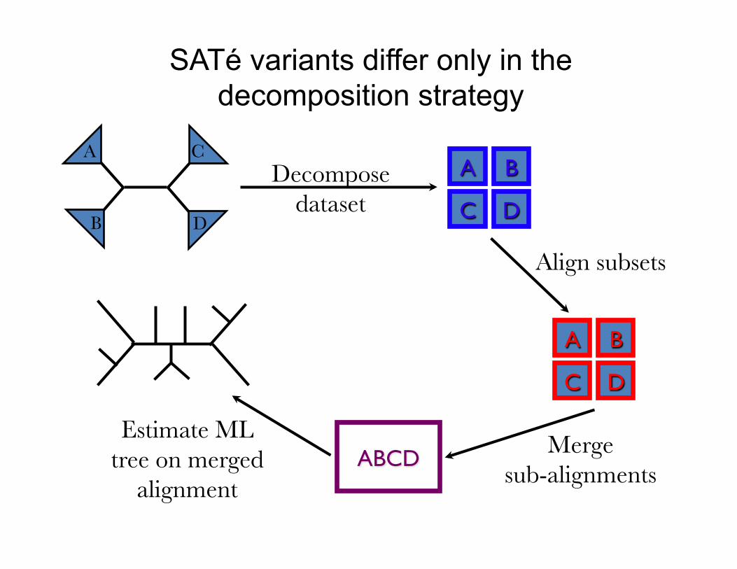
SATé variants differ only in the decomposition strategy
A
B D
C
Merge sub-alignments
Estimate ML tree on merged
alignment
Decompose dataset
A B
C D
Align subsets
A B
C D
ABCD
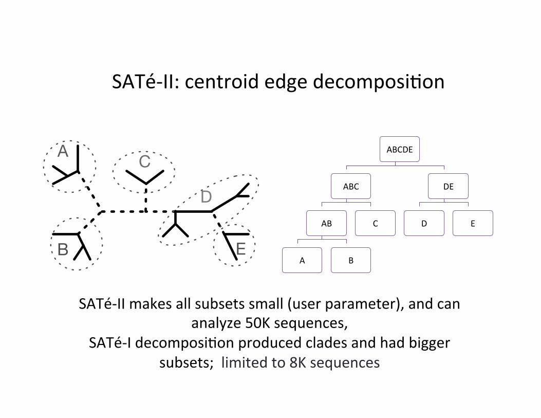
SATé-‐II: centroid edge decomposi,on
A
B
C
D
E
ABCDE
ABC
AB
A B
C
DE
D E
SATé-‐II makes all subsets small (user parameter), and can analyze 50K sequences,
SATé-‐I decomposi,on produced clades and had bigger subsets; limited to 8K sequences
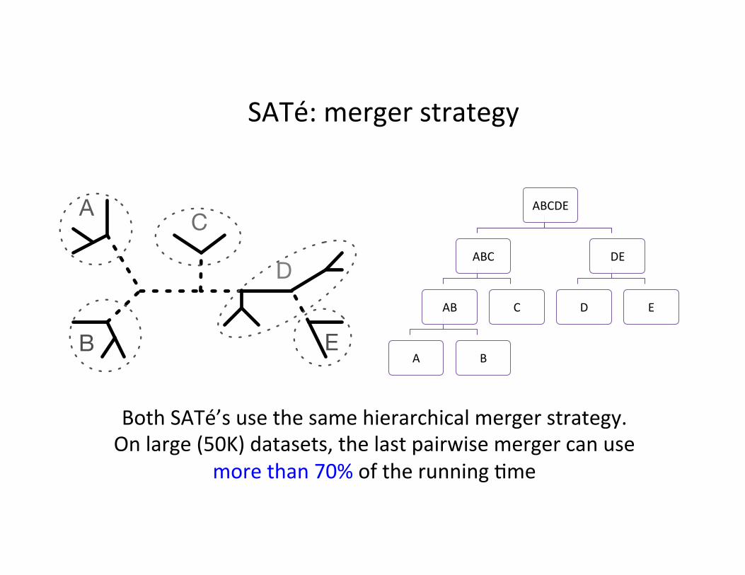
SATé: merger strategy
A
B
C
D
E
ABCDE
ABC
AB
A B
C
DE
D E
Both SATé’s use the same hierarchical merger strategy. On large (50K) datasets, the last pairwise merger can use
more than 70% of the running ,me
A
B
C
D
E
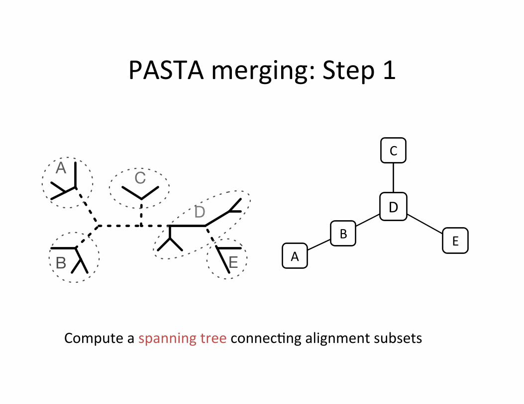
PASTA merging: Step 1
D
C
E B A
Compute a spanning tree connec,ng alignment subsets
A
B
C
D
E
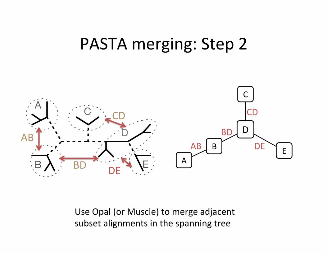
PASTA merging: Step 2
D
C
E B A
AB
BD
CD
DE
AB BD
CD
DE
Use Opal (or Muscle) to merge adjacent subset alignments in the spanning tree
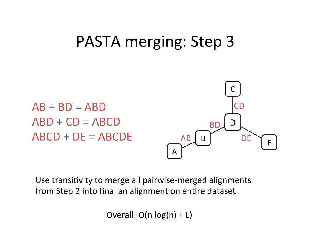
PASTA merging: Step 3
D
C
E B A
Use transi,vity to merge all pairwise-‐merged alignments from Step 2 into final an alignment on en,re dataset
AB + BD = ABD ABD + CD = ABCD ABCD + DE = ABCDE
AB BD
CD
DE
Overall: O(n log(n) + L)
�
�
�
�
�
� � � � � �� ������ � �������
�������
�����
PASTA vs. SATé-‐II profiling and scaling 10 PASTA: ultra-large multiple sequence alignment
(a)
●
●
●
●
●
●
●
●
0
250
500
750
1000
1250
10,000 50,000 100,000 200,000Number of Sequences
Run
ning
tim
e (m
inut
es)
(b)
●●
●●
●
●
●
●
●
●
●
●
●
●
1
2
4
6
8
1 2 4 6 8 10 12Number of Threads
Spee
dup
●
●
PASTASATe2
(c)
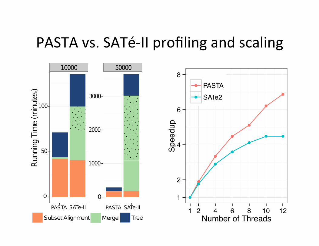
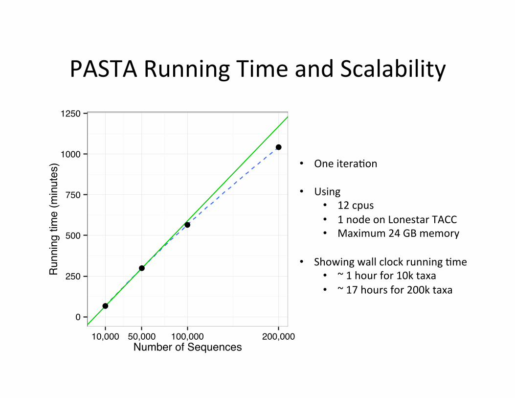
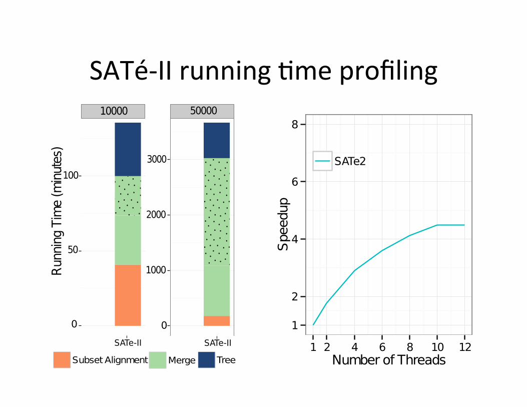
Fig. 5. Running time comparison of PASTA and SATe. (a) Running time pro-filing on one iteration for RNASim datasets with 10K and 50K sequences (the dottedregion indicates the last pairwise merge). (b) Running time for one iteration of PASTAwith 12 CPUs as a function of the number of sequences (the solid line is fitted to firsttwo points). (c) Scalability for PASTA and SATe with increased number of CPUs.
reason SATe uses so much time is that all mergers are done hierarchically usingeither Opal (for small datasets) or Muscle (on larger datasets), and both arecomputationally expensive with increased number of sequences. For example,the last pairwise merge within SATe, shown by the dotted area in Figure 5a,is entirely serial and takes up a large chunk of the total time. PASTA solvesthis problem by using transitivity for all but the initial pairwise mergers, andtherefore scales well with increased dataset size, as shown in Figure 5b (thesub-linear scaling is due to a better use of parallelism with increased number ofsequences). Finally, Figure 5c shows that PASTA is highly parallelizable, andhas a much better speed-up with increasing number of threads than SATe does.While PASTA has a much improved parallelization, it does not quite scale uplinearly, because FastTree-2 does not scale up well with increased thread count.
Divide-and-Conquer strategy: impact of guide tree. We also investigated theimpact of the use of the guide tree for computing the subset decomposition,and hence defining the Type 1 sub-alignments. We compared results obtainedusing three di↵erent decompositions: the decomposition computed by PASTAon the HMM-based starting tree, the decomposition computed by PASTA onthe true (model) tree, and a random decomposition into subsets of size 200,all on the RNASim 10k dataset. PASTA alignments and trees had roughly thesame accuracy when the guide tree was either the true tree or the HMM-basedstarting tree (Table 3). However, when based on a random decomposition, treeerror increased dramatically from 10.5% to 52.3%, and alignment scores alsodropped substantially. Thus, the guide-tree based dataset decomposition usedby PASTA provides substantial improvements over random decompositions, andthe default technique for getting the starting tree works quite well.
����� �����
�
��
���
�
����
����
����
�����
�� ����� ��
� � ���� ����� �� ��
����� ��� �������� ��� ���
PASTA Running Time and Scalability 10 PASTA: ultra-large multiple sequence alignment
(a)
●
●
●
●
●
●
●
●
0
250
500
750
1000
1250
10,000 50,000 100,000 200,000Number of Sequences
Run
ning
tim
e (m
inut
es)
(b)
●●
●●
●
●
●
●
●
●
●
●
●
●
1
2
4
6
8
1 2 4 6 8 10 12Number of Threads
Spee
dup
●
●
PASTASATe2
(c)
Fig. 5. Running time comparison of PASTA and SATe. (a) Running time pro-filing on one iteration for RNASim datasets with 10K and 50K sequences (the dottedregion indicates the last pairwise merge). (b) Running time for one iteration of PASTAwith 12 CPUs as a function of the number of sequences (the solid line is fitted to firsttwo points). (c) Scalability for PASTA and SATe with increased number of CPUs.
reason SATe uses so much time is that all mergers are done hierarchically usingeither Opal (for small datasets) or Muscle (on larger datasets), and both arecomputationally expensive with increased number of sequences. For example,the last pairwise merge within SATe, shown by the dotted area in Figure 5a,is entirely serial and takes up a large chunk of the total time. PASTA solvesthis problem by using transitivity for all but the initial pairwise mergers, andtherefore scales well with increased dataset size, as shown in Figure 5b (thesub-linear scaling is due to a better use of parallelism with increased number ofsequences). Finally, Figure 5c shows that PASTA is highly parallelizable, andhas a much better speed-up with increasing number of threads than SATe does.While PASTA has a much improved parallelization, it does not quite scale uplinearly, because FastTree-2 does not scale up well with increased thread count.
Divide-and-Conquer strategy: impact of guide tree. We also investigated theimpact of the use of the guide tree for computing the subset decomposition,and hence defining the Type 1 sub-alignments. We compared results obtainedusing three di↵erent decompositions: the decomposition computed by PASTAon the HMM-based starting tree, the decomposition computed by PASTA onthe true (model) tree, and a random decomposition into subsets of size 200,all on the RNASim 10k dataset. PASTA alignments and trees had roughly thesame accuracy when the guide tree was either the true tree or the HMM-basedstarting tree (Table 3). However, when based on a random decomposition, treeerror increased dramatically from 10.5% to 52.3%, and alignment scores alsodropped substantially. Thus, the guide-tree based dataset decomposition usedby PASTA provides substantial improvements over random decompositions, andthe default technique for getting the starting tree works quite well.
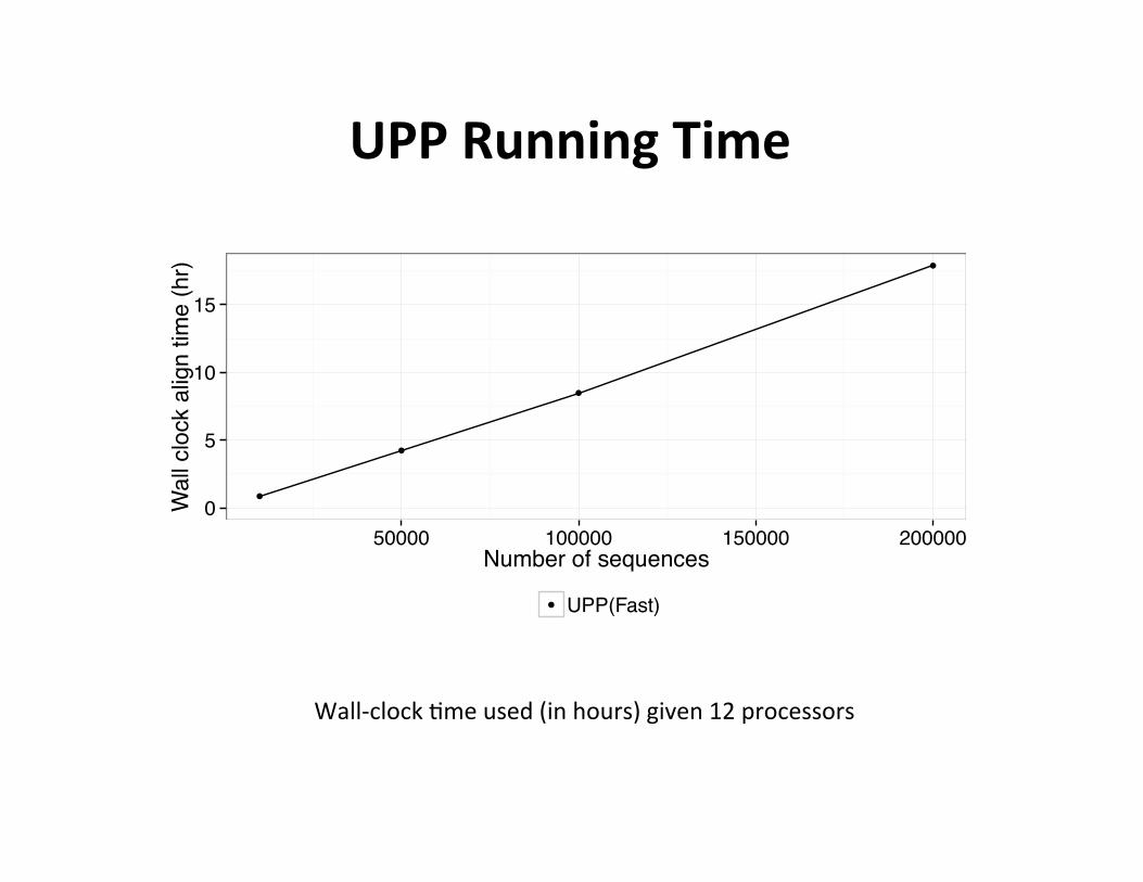
• One itera,on
• Using • 12 cpus • 1 node on Lonestar TACC • Maximum 24 GB memory
• Showing wall clock running ,me • ~ 1 hour for 10k taxa • ~ 17 hours for 200k taxa
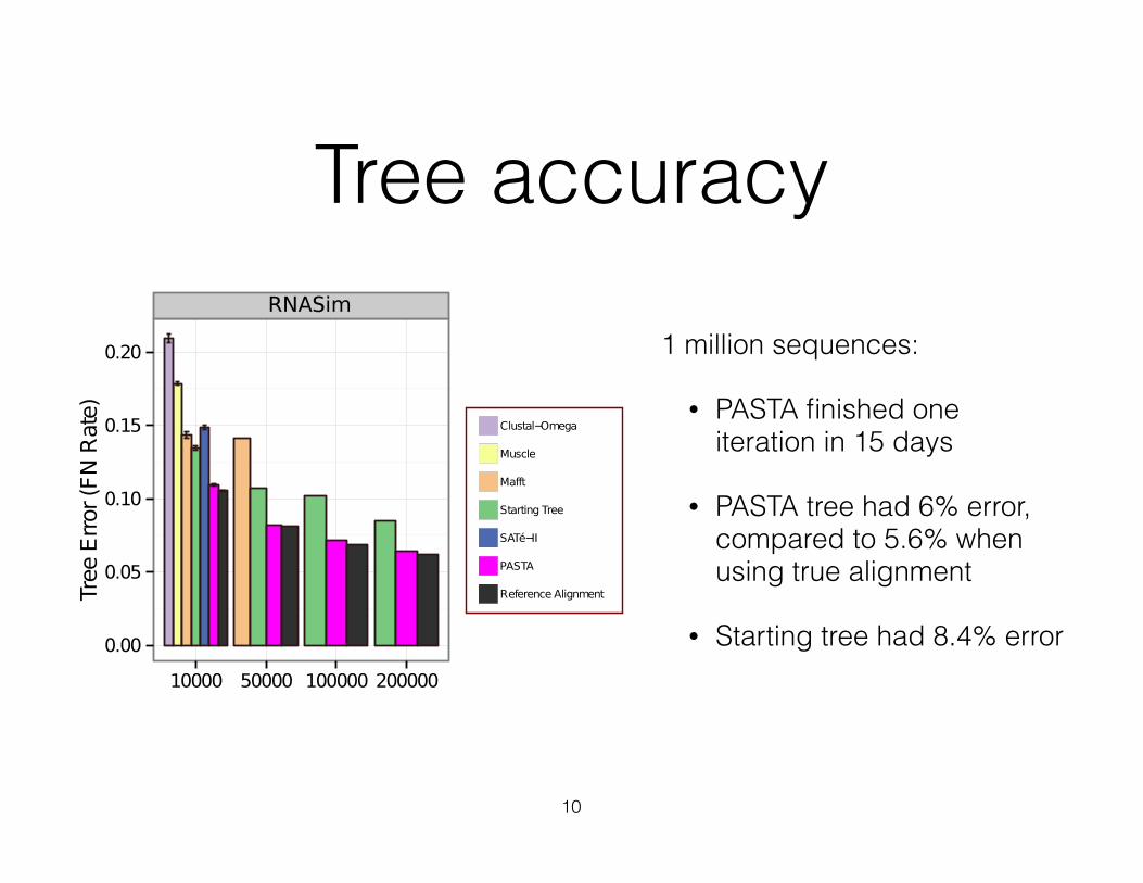
Tree accuracy
10
Figure 3.3: Tree error rates on nucleotide datasets. We show missingbranch (also known as false negative or FN) rates for maximum likelihood treesestimated using FastTree-II, on the reference alignment as well as alignmentscomputed using PASTA and other methods; results not shown indicate failureto complete within 24 hours using 12 cores on the datasets. Error bars showstandard error over 10 replicates for all model conditions of the Indelible andthe 10,000-sequence RNASim datasets.
82
1 million sequences:
• PASTA finished one iteration in 15 days
• PASTA tree had 6% error, compared to 5.6% when using true alignment
• Starting tree had 8.4% error
PASTA vs. SATé-‐II • Difference is how subset alignments are merged together (transi,vity instead of Opal/Muscle).
• As expected, PASTA is faster and can analyze larger datasets.
• Unexpected: PASTA produces more accurate alignments and trees (on both simulated and biological data, including DNA, RNA, and AA sequences).
• Thus, transi,vity applied to compa,ble and overlapping alignments gives a surprisingly accurate technique for merging a collec,on of alignments.
PASTA and SATé-‐II: MSA “boosters”
• PASTA and SATé-‐II are techniques for improving the scalability of MSA methods to large datasets.
• We showed results here using MAFFT-‐l-‐ins-‐i to align small subsets with 200 sequences.
• We have also explored results using other MSA methods (e.g., Prank, Clustal, Bali-‐Phy), and obtain similar improvements in accuracy and/or scalability.
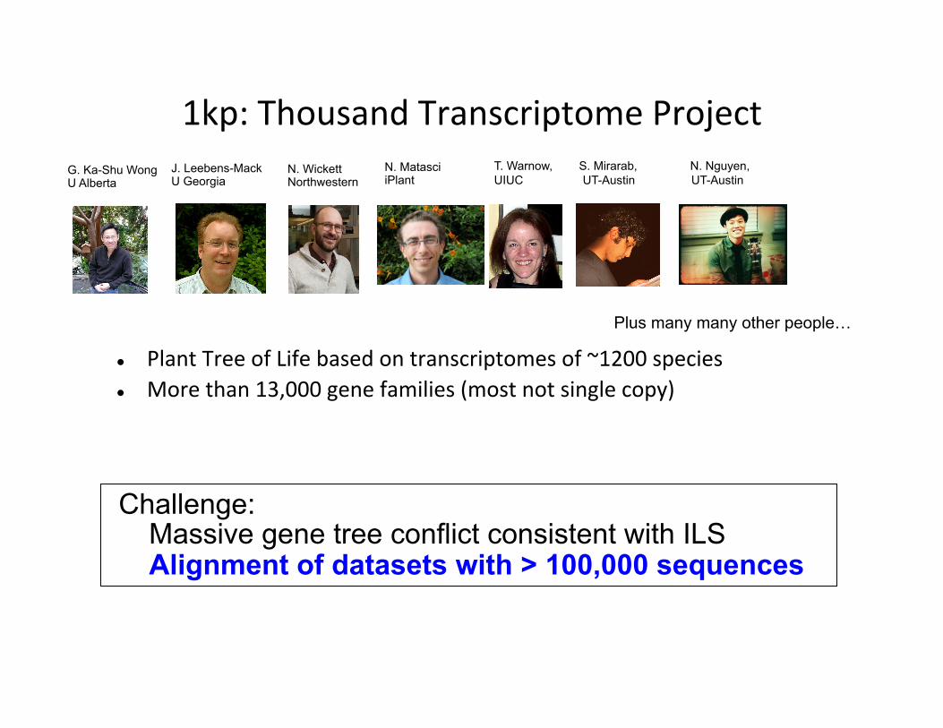
1kp: Thousand Transcriptome Project
l Plant Tree of Life based on transcriptomes of ~1200 species l More than 13,000 gene families (most not single copy) Gene Tree Incongruence
G. Ka-Shu Wong U Alberta
N. Wickett Northwestern
J. Leebens-Mack U Georgia
N. Matasci iPlant
T. Warnow, S. Mirarab, N. Nguyen, UIUC UT-Austin UT-Austin
Challenge: Massive gene tree conflict consistent with ILS Alignment of datasets with > 100,000 sequences
Plus many many other people…
Length
Counts
0
2000
4000
6000
8000
10000
12000 Mean:317Median:266
0 500 1000 1500 2000
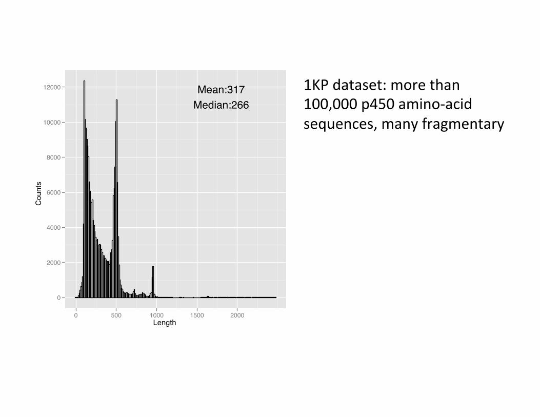
1KP dataset: more than 100,000 p450 amino-‐acid sequences, many fragmentary
Length
Counts
0
2000
4000
6000
8000
10000
12000 Mean:317Median:266
0 500 1000 1500 2000
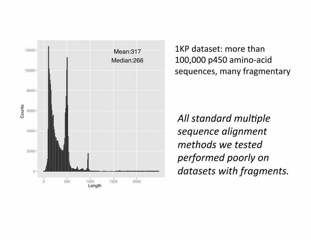
1KP dataset: more than 100,000 p450 amino-‐acid sequences, many fragmentary
All standard mul>ple sequence alignment methods we tested performed poorly on datasets with fragments.
1kp: Thousand Transcriptome Project
l Plant Tree of Life based on transcriptomes of ~1200 species l More than 13,000 gene families (most not single copy) Gene Tree Incongruence
G. Ka-Shu Wong U Alberta
N. Wickett Northwestern
J. Leebens-Mack U Georgia
N. Matasci iPlant
T. Warnow, S. Mirarab, N. Nguyen UIUC UT-Austin UT-Austin
Challenge: Alignment of datasets with > 100,000 sequences with many fragmentary sequences
Plus many many other people…
UPP UPP = “Ultra-‐large mul,ple sequence alignment using Phylogeny-‐aware Profiles” Nguyen, Mirarab, and Warnow. Genome Biology, 2014. Purpose: highly accurate large-‐scale mul,ple sequence alignments, even in the presence of fragmentary sequences.
UPP UPP = “Ultra-‐large mul,ple sequence alignment using Phylogeny-‐aware Profiles” Nguyen, Mirarab, and Warnow. Genome Biology, 2014. Purpose: highly accurate large-‐scale mul,ple sequence alignments, even in the presence of fragmentary sequences.
Uses an ensemble of HMMs

Simple idea (not UPP)
• Select random subset of sequences, and build “backbone alignment”
• Construct a Hidden Markov Model (HMM) on the backbone alignment
• Add all remaining sequences to the backbone alignment using the HMM

One Hidden Markov Model for the entire alignment?
Simple idea (not UPP)
• Select random subset of sequences, and build “backbone alignment”
• Construct a Hidden Markov Model (HMM) on the backbone alignment
• Add all remaining sequences to the backbone alignment using the HMM
• Select random subset of sequences, and build “backbone alignment”
• Construct a Hidden Markov Model (HMM) on the backbone alignment
• Add all remaining sequences to the backbone alignment using the HMM
This approach works well if the dataset is small and has low evolu,onary rates, but is not very accurate otherwise.
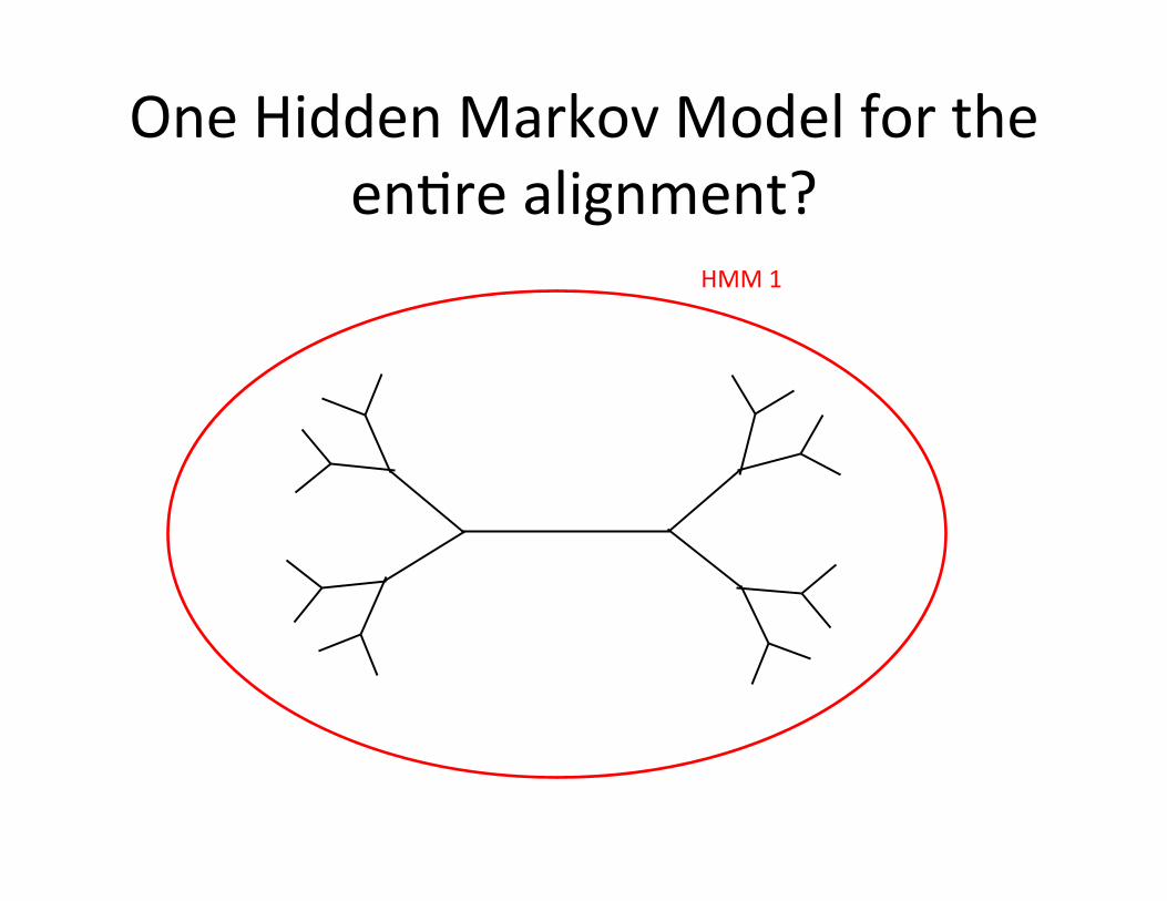
One Hidden Markov Model for the en,re alignment?
HMM 1
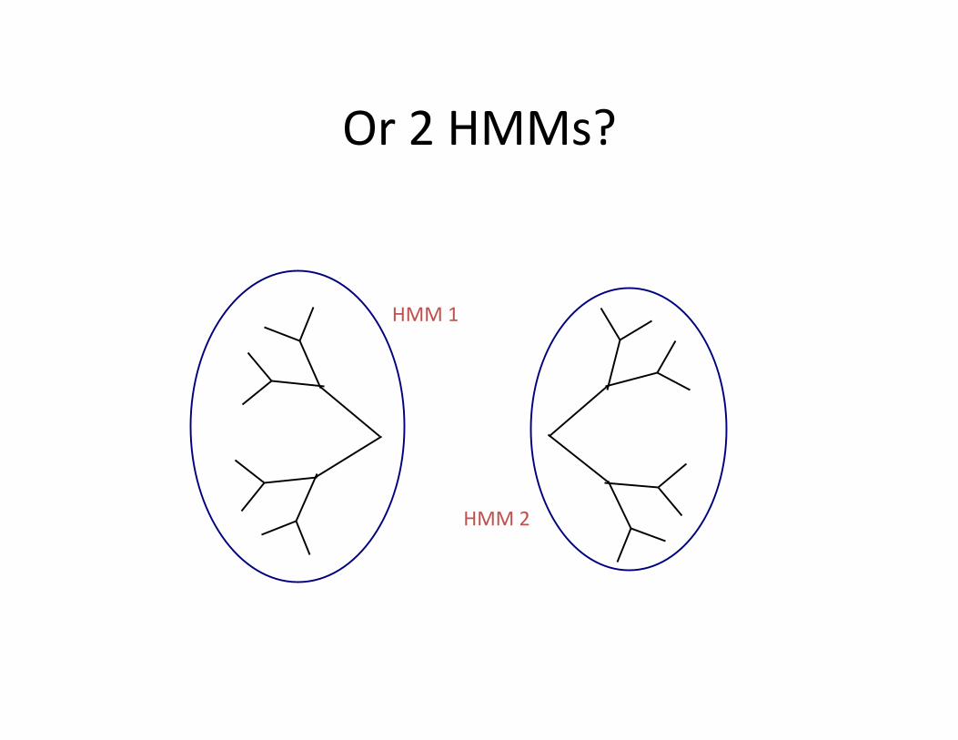
Or 2 HMMs?
HMM 1
HMM 2
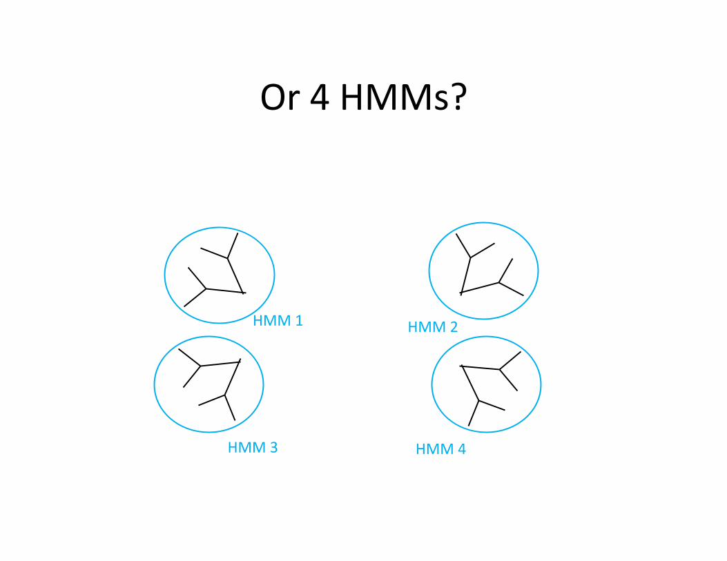
HMM 1
HMM 3 HMM 4
HMM 2
Or 4 HMMs?
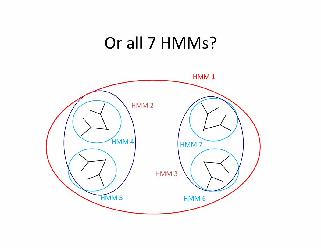
m
HMM 2
HMM 3
HMM 1
HMM 4
HMM 5 HMM 6
HMM 7
Or all 7 HMMs?
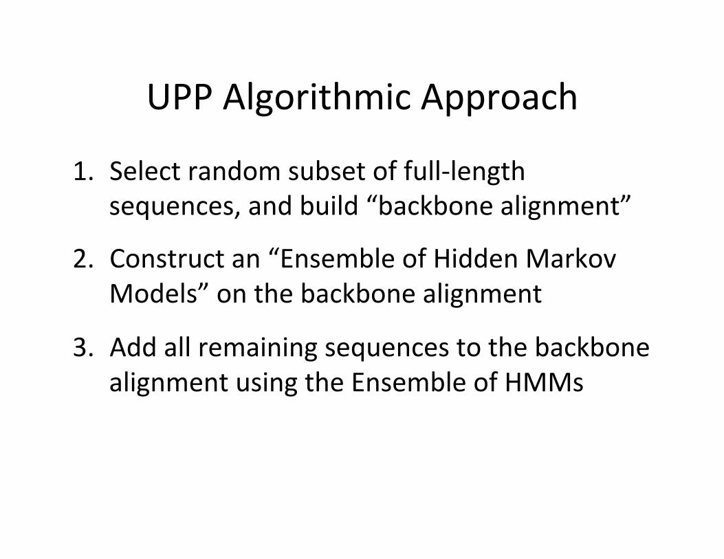
UPP Algorithmic Approach
1. Select random subset of full-‐length sequences, and build “backbone alignment”
2. Construct an “Ensemble of Hidden Markov Models” on the backbone alignment
3. Add all remaining sequences to the backbone alignment using the Ensemble of HMMs
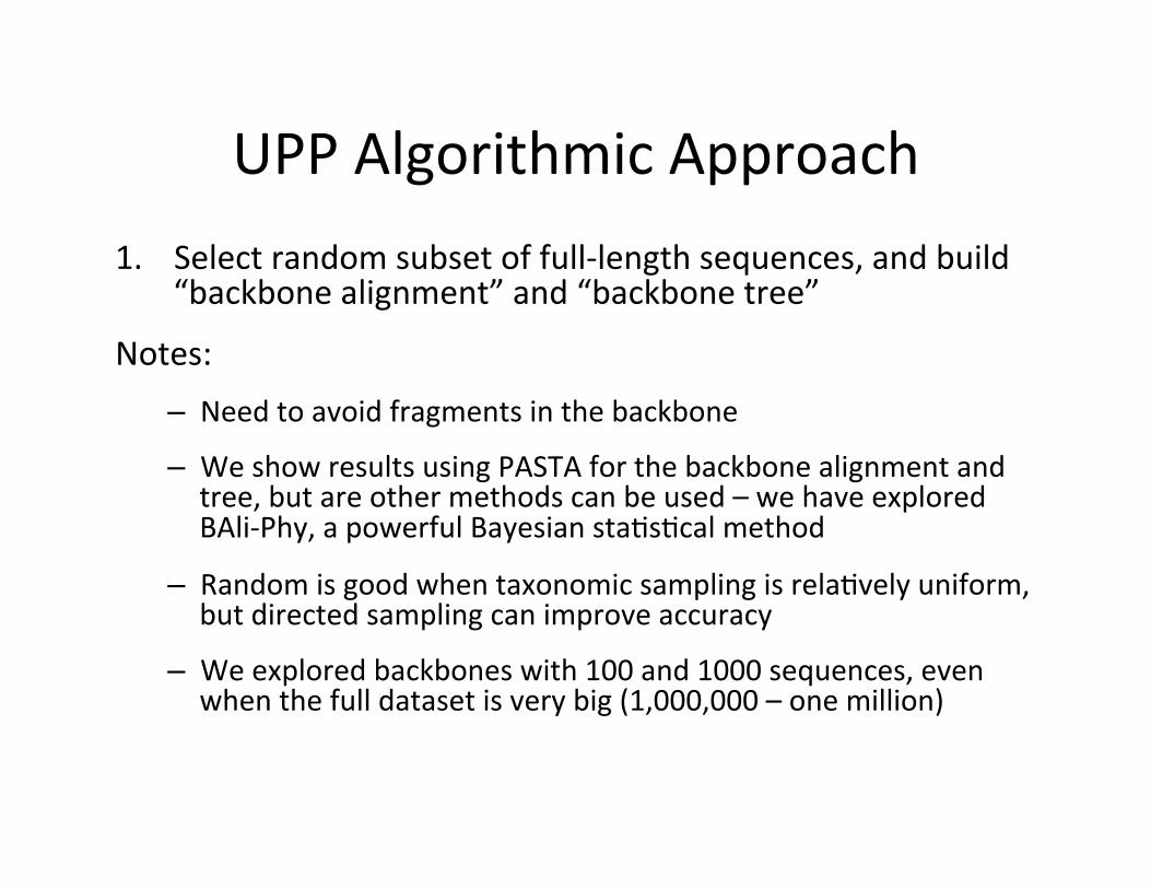
UPP Algorithmic Approach 1. Select random subset of full-‐length sequences, and build
“backbone alignment” and “backbone tree”
Notes: – Need to avoid fragments in the backbone
– We show results using PASTA for the backbone alignment and tree, but are other methods can be used – we have explored BAli-‐Phy, a powerful Bayesian sta,s,cal method
– Random is good when taxonomic sampling is rela,vely uniform, but directed sampling can improve accuracy
– We explored backbones with 100 and 1000 sequences, even when the full dataset is very big (1,000,000 – one million)
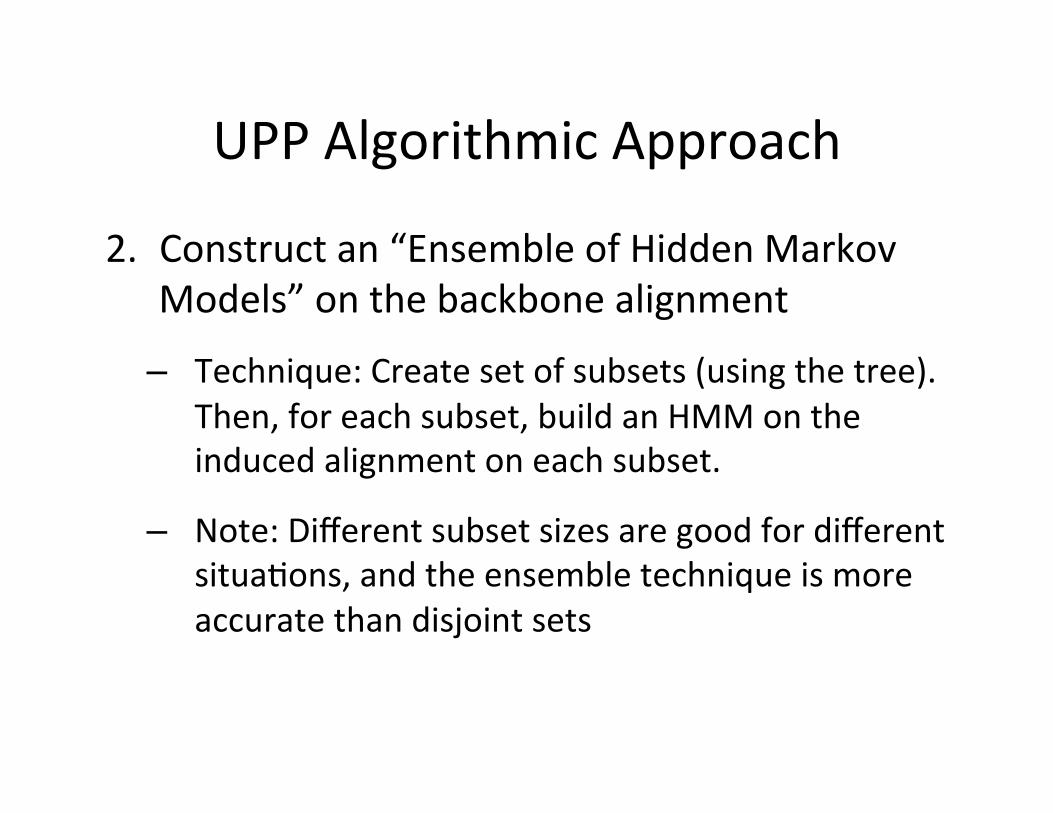
UPP Algorithmic Approach
2. Construct an “Ensemble of Hidden Markov Models” on the backbone alignment
– Technique: Create set of subsets (using the tree). Then, for each subset, build an HMM on the induced alignment on each subset.
– Note: Different subset sizes are good for different situa,ons, and the ensemble technique is more accurate than disjoint sets
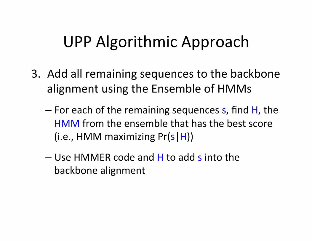
UPP Algorithmic Approach
3. Add all remaining sequences to the backbone alignment using the Ensemble of HMMs
– For each of the remaining sequences s, find H, the HMM from the ensemble that has the best score (i.e., HMM maximizing Pr(s|H))
– Use HMMER code and H to add s into the backbone alignment
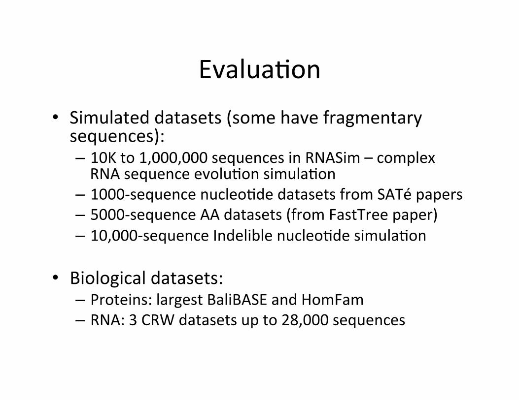
Evalua,on • Simulated datasets (some have fragmentary sequences): – 10K to 1,000,000 sequences in RNASim – complex RNA sequence evolu,on simula,on
– 1000-‐sequence nucleo,de datasets from SATé papers – 5000-‐sequence AA datasets (from FastTree paper) – 10,000-‐sequence Indelible nucleo,de simula,on
• Biological datasets: – Proteins: largest BaliBASE and HomFam – RNA: 3 CRW datasets up to 28,000 sequences
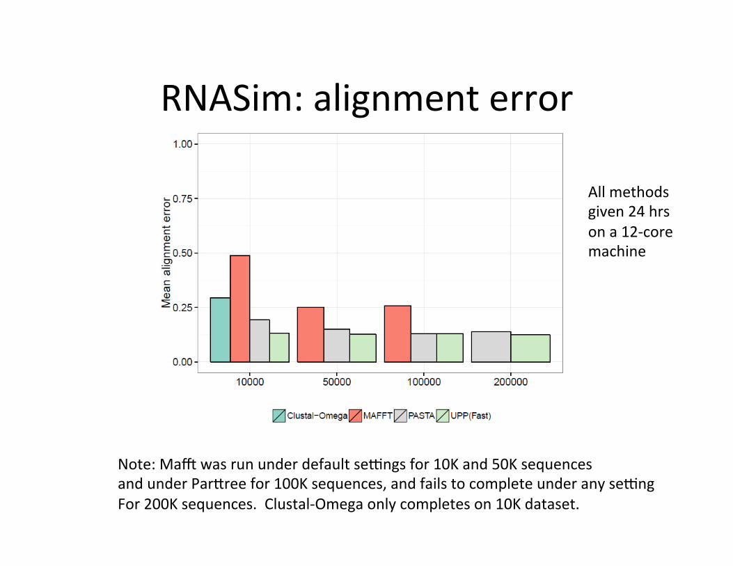
RNASim: alignment error
Note: Maz was run under default se{ngs for 10K and 50K sequences and under ParEree for 100K sequences, and fails to complete under any se{ng For 200K sequences. Clustal-‐Omega only completes on 10K dataset.
All methods given 24 hrs on a 12-‐core machine
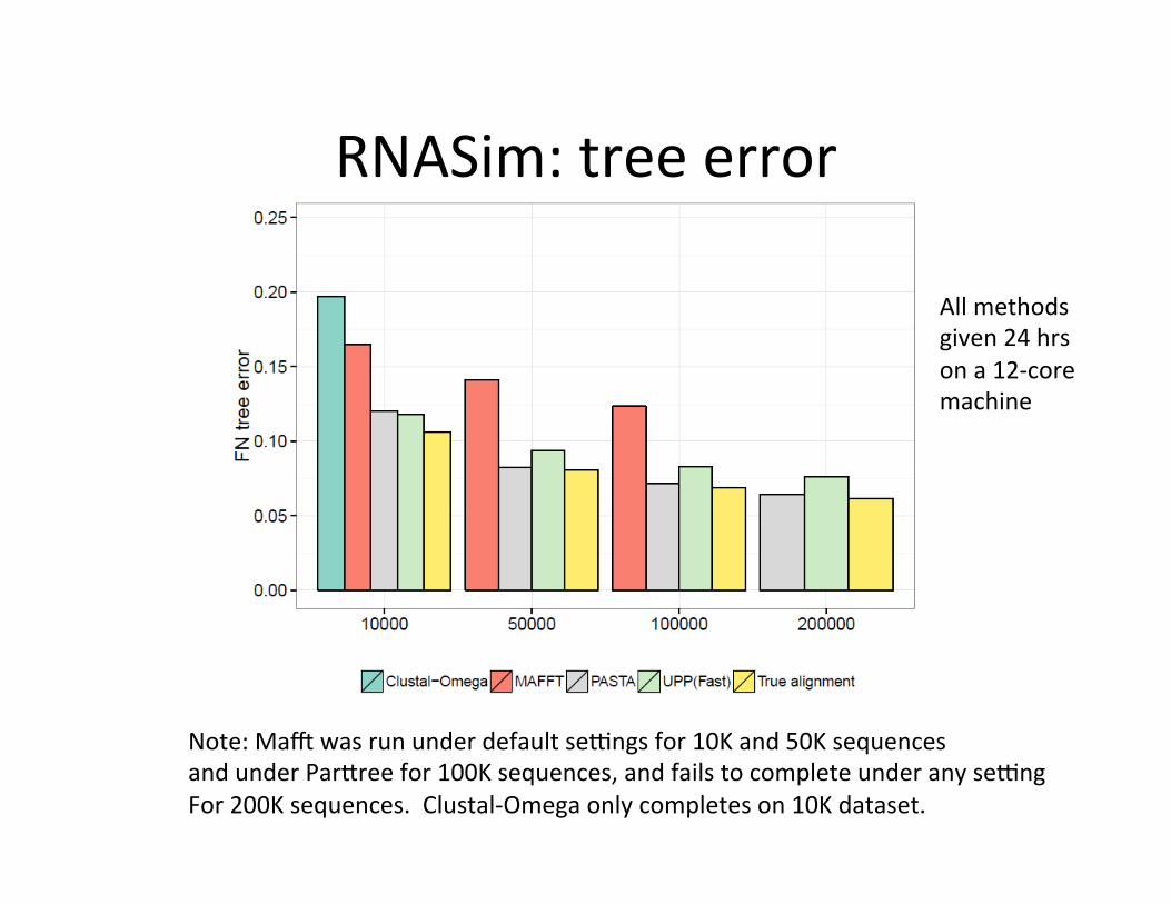
RNASim: tree error
Note: Maz was run under default se{ngs for 10K and 50K sequences and under ParEree for 100K sequences, and fails to complete under any se{ng For 200K sequences. Clustal-‐Omega only completes on 10K dataset.
All methods given 24 hrs on a 12-‐core machine
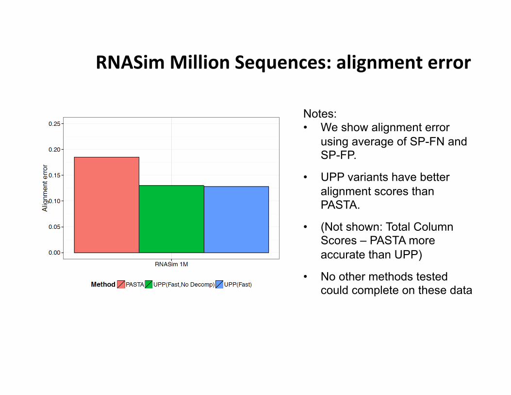
RNASim Million Sequences: alignment error
Notes: • We show alignment error
using average of SP-FN and SP-FP.
• UPP variants have better alignment scores than PASTA.
• (Not shown: Total Column Scores – PASTA more accurate than UPP)
• No other methods tested could complete on these data
• PASTA under-aligns: its alignment is 43 times wider than true alignment (~900 Gb of disk space). UPP alignments were closer in length to true alignment (0.93 to 1.38 wider).
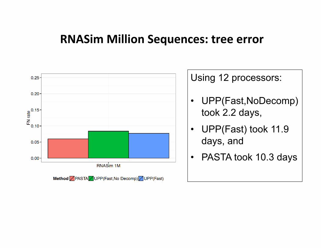
RNASim Million Sequences: tree error
Using 12 processors: • UPP(Fast,NoDecomp)
took 2.2 days,
• UPP(Fast) took 11.9 days, and
• PASTA took 10.3 days
0.0
0.2
0.4
0.6
0 12.5 25 50% Fragmentary
Mea
n al
ignm
ent e
rror
PASTA UPP(Default)
(a) Average alignment error
0.0
0.2
0.4
0 12.5 25 50% Fragmentary
Del
ta F
N tr
ee e
rror
PASTA UPP(Default)
(b) Average tree error
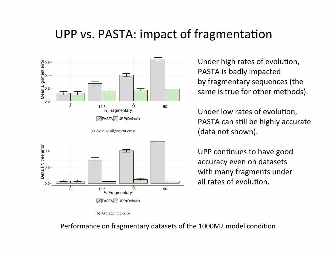
Figure S32: Alignment and tree error of PASTA and UPP on the fragmentary 1000M2datasets.
80
Performance on fragmentary datasets of the 1000M2 model condi,on
UPP vs. PASTA: impact of fragmenta,on
Under high rates of evolu,on, PASTA is badly impacted by fragmentary sequences (the same is true for other methods). Under low rates of evolu,on, PASTA can s,ll be highly accurate (data not shown). UPP con,nues to have good accuracy even on datasets with many fragments under all rates of evolu,on.
●
●
●
●
0
5
10
15
50000 100000 150000 200000Number of sequences
Wal
l clo
ck a
lign
time
(hr)
● UPP(Fast)
UPP Running Time
Wall-‐clock ,me used (in hours) given 12 processors
Current Related Research UPP: • Using itera,on • Using other MSA models (not just HMMs) within the “Ensemble” • Using structural alignments for the backbone • Using powerful sta,s,cal methods to produce the backbone alignment and tree
PASTA : • Using powerful sta,s,cal methods for the subset alignments • Improving the pairwise merging technique
ENSEMBLE OF HMMS: • Metagenomic taxon iden,fica,on (collabora,on with Mihai Pop, Maryland) • Gene binning (joint with Jian Peng, UIUC, and with Jim Leebens-‐Mack, Georgia) • Protein structure and func,on classifica,on (collabora,ons with Mar,n Weigt, Paris, and
Jian Peng, UIUC)
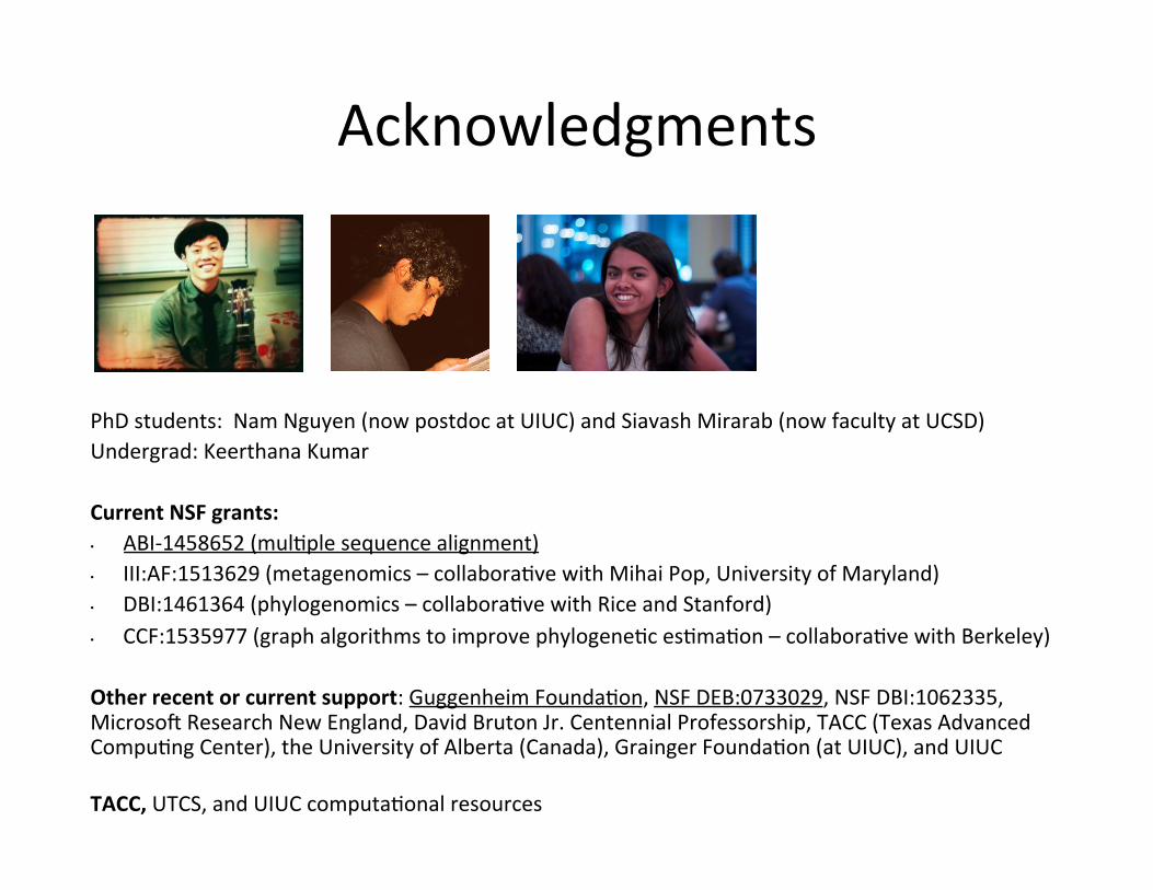
Acknowledgments
PhD students: Nam Nguyen (now postdoc at UIUC) and Siavash Mirarab (now faculty at UCSD) Undergrad: Keerthana Kumar Current NSF grants: • ABI-‐1458652 (mul,ple sequence alignment) • III:AF:1513629 (metagenomics – collabora,ve with Mihai Pop, University of Maryland) • DBI:1461364 (phylogenomics – collabora,ve with Rice and Stanford) • CCF:1535977 (graph algorithms to improve phylogene,c es,ma,on – collabora,ve with Berkeley) Other recent or current support: Guggenheim Founda,on, NSF DEB:0733029, NSF DBI:1062335, Microso` Research New England, David Bruton Jr. Centennial Professorship, TACC (Texas Advanced Compu,ng Center), the University of Alberta (Canada), Grainger Founda,on (at UIUC), and UIUC TACC, UTCS, and UIUC computa,onal resources
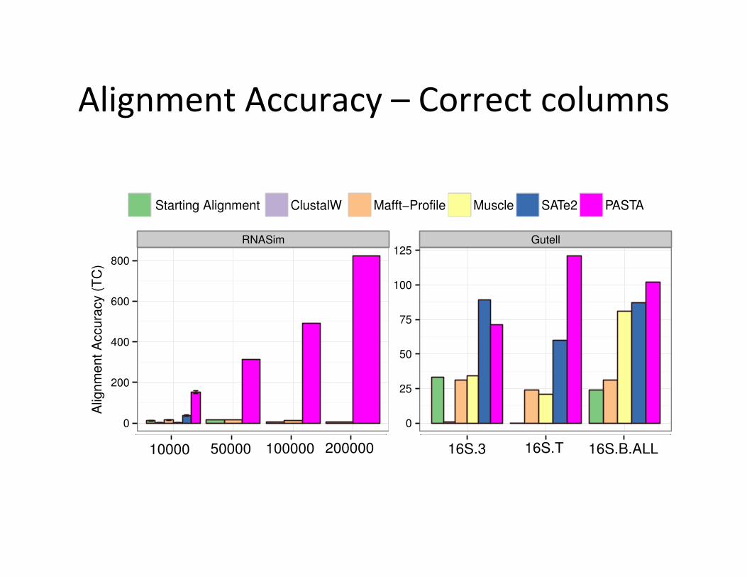
Alignment Accuracy – Correct columns 8 PASTA: ultra-large multiple sequence alignment
RNASim Gutell
0
200
400
600
800
0
25
50
75
100
125
Alig
nmen
tAcc
urac
y(T
C)
Starting Alignment ClustalW Mafft"Profile Muscle SATe2 PASTA
Fig. 3. Alignment accuracy on the RNASim 10K-200K (left) and biological
(right) datasets. We show the number of correctly aligned sites (top) and the averageof the SP-score and modeler score (bottom). The starting alignment was incomplete onthe 16S.T dataset, and so no result is shown for the starting alignment on that dataset.
were recovered entirely correctly. Another interesting trend is that as the numberof sequences increases, the alignment accuracy decreased for MAFFT-profile butnot for PASTA.
The biological datasets are smaller (see Table 1) and so are not as challenging.On the 16S.T dataset, the starting alignment did not return an alignment withall the sequences on the 16S.T dataset because HMMER considered one of thesequences unalignable. However, the starting alignment technique had good SP-scores for the other two datasets. Of the remaining methods, PASTA has thebest sum-of-pairs scores (bottom panel), and MAFFT-profile has only slightlypoorer scores; the other methods are substantially poorer. With respect to TCscores, on 16S.B.ALL and 16S.T, PASTA is in first place and SATe is in secondplace, but they swap positions on 16S.3. TC scores for the other methods areclearly less accurate, though Muscle does fairly well on the 16S.B.ALL dataset.
Comparison to SATe on 50,000 taxon dataset. SATe could not finish even oneiteration on the RNASim with 50,000 sequences running for 24 hours and given12 CPUs on TACC. However, we were able to run two iterations of SATe on aseparate machine with no running time limits (12 Quad-Core AMD Opteron(tm)processors, 256GB of RAM memory). Given 12 CPUs, each iteration of SATetakes roughly 70 hours, compared to 5 hours for PASTA, and as shown next, the
8 PASTA: ultra-large multiple sequence alignment
0.00 0.00
10000 50000 100000 200000 16S.3 16S.T 16S.B.ALL
Fig. 3. Alignment accuracy on the RNASim 10K-200K (left) and biological
(right) datasets. We show the number of correctly aligned sites (top) and the averageof the SP-score and modeler score (bottom). The starting alignment was incomplete onthe 16S.T dataset, and so no result is shown for the starting alignment on that dataset.
were recovered entirely correctly. Another interesting trend is that as the numberof sequences increases, the alignment accuracy decreased for MAFFT-profile butnot for PASTA.
The biological datasets are smaller (see Table 1) and so are not as challenging.On the 16S.T dataset, the starting alignment did not return an alignment withall the sequences on the 16S.T dataset because HMMER considered one of thesequences unalignable. However, the starting alignment technique had good SP-scores for the other two datasets. Of the remaining methods, PASTA has thebest sum-of-pairs scores (bottom panel), and MAFFT-profile has only slightlypoorer scores; the other methods are substantially poorer. With respect to TCscores, on 16S.B.ALL and 16S.T, PASTA is in first place and SATe is in secondplace, but they swap positions on 16S.3. TC scores for the other methods areclearly less accurate, though Muscle does fairly well on the 16S.B.ALL dataset.
Comparison to SATe on 50,000 taxon dataset. SATe could not finish even oneiteration on the RNASim with 50,000 sequences running for 24 hours and given12 CPUs on TACC. However, we were able to run two iterations of SATe on aseparate machine with no running time limits (12 Quad-Core AMD Opteron(tm)processors, 256GB of RAM memory). Given 12 CPUs, each iteration of SATetakes roughly 70 hours, compared to 5 hours for PASTA, and as shown next, the
TIPP: high accuracy taxonomic identification of metagenomic data
TIPP: taxon identification and phylogenetic profiling
(Bioinformatics, 2014) Technique: combines UPP alignments and phylogenetic
placement algorithms, and considers statistical uncertainty.
Results: better accuracy than all current methods, even for
sequencing technologies producing high indel rates Research funded by new NSF grant III:AF:1513629
(collabora,ve with Mihai Pop at University of Maryland)
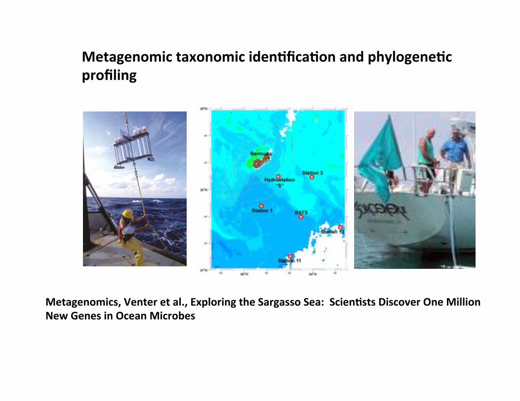
Metagenomic taxonomic iden*fica*on and phylogene*c profiling
Metagenomics, Venter et al., Exploring the Sargasso Sea: Scien*sts Discover One Million New Genes in Ocean Microbes

1. What is this fragment? (Classify each fragment as well as possible.)
2. What is the taxonomic distribu,on in the dataset? (Note: helpful to use marker genes.)
3. What are the organisms in this metagenomic sample doing together?
Basic Ques,ons
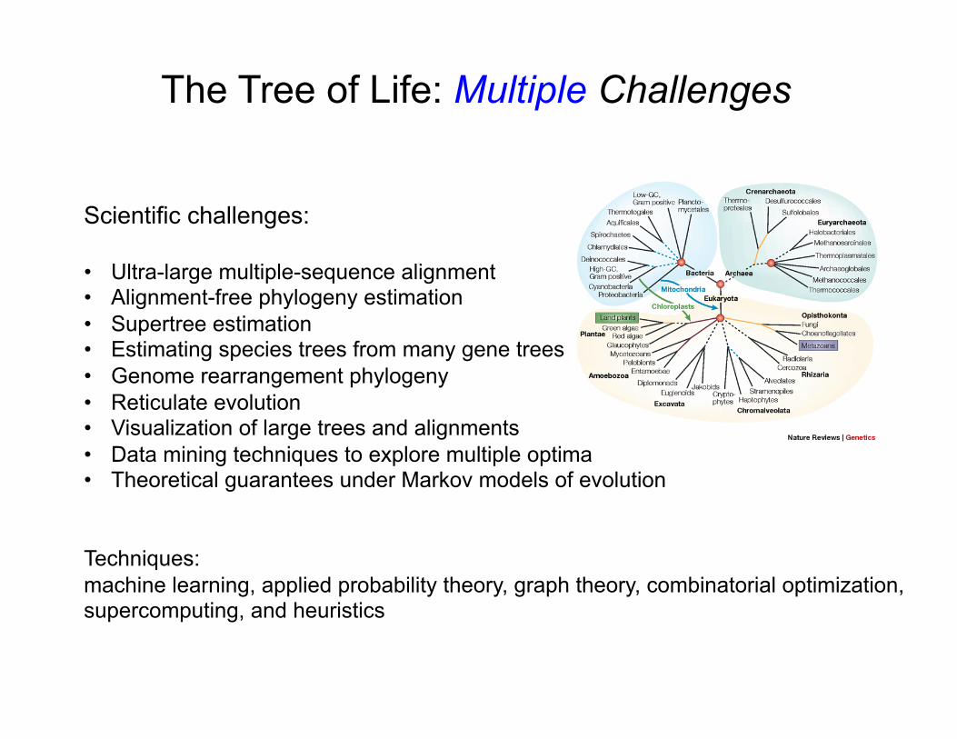
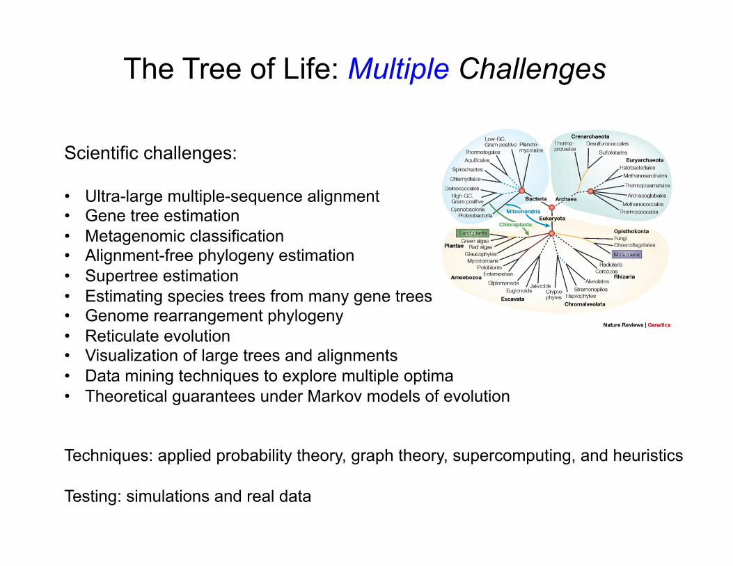
Scientific challenges: • Ultra-large multiple-sequence alignment • Alignment-free phylogeny estimation • Supertree estimation • Estimating species trees from many gene trees • Genome rearrangement phylogeny • Reticulate evolution • Visualization of large trees and alignments • Data mining techniques to explore multiple optima • Theoretical guarantees under Markov models of evolution
Techniques: machine learning, applied probability theory, graph theory, combinatorial optimization, supercomputing, and heuristics
The Tree of Life: Multiple Challenges
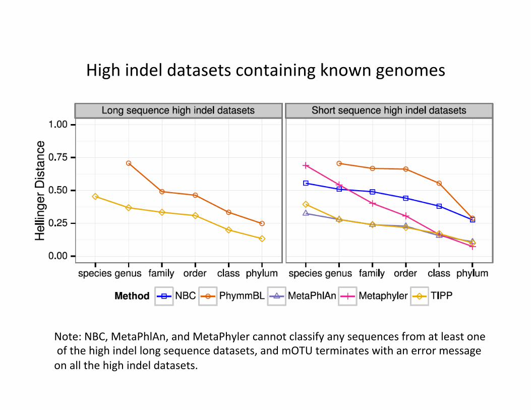
High indel datasets containing known genomes
Note: NBC, MetaPhlAn, and MetaPhyler cannot classify any sequences from at least one of the high indel long sequence datasets, and mOTU terminates with an error message on all the high indel datasets.
TIPP vs. other abundance profilers • TIPP is highly accurate, even in the presence of high indel rates and novel genomes, and for both short and long reads.
• All other methods have some vulnerability (e.g., mOTU is only accurate for short reads and is impacted by high indel rates).
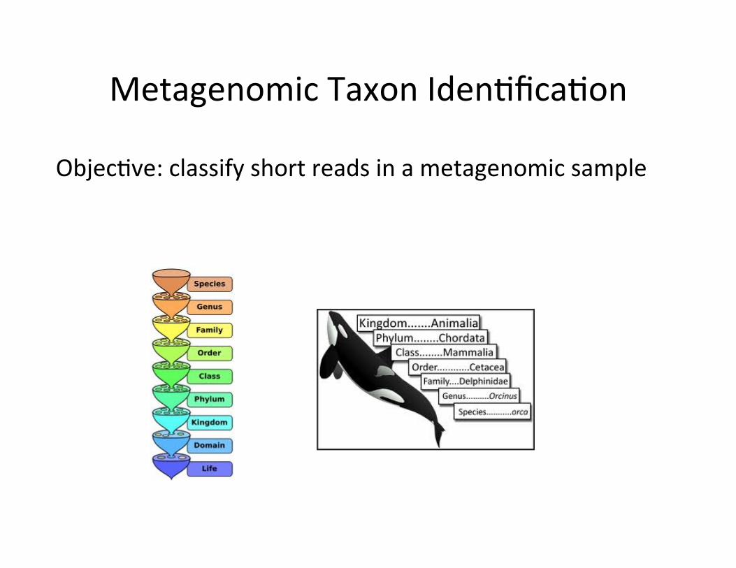
Metagenomic Taxon Iden,fica,on Objec,ve: classify short reads in a metagenomic sample
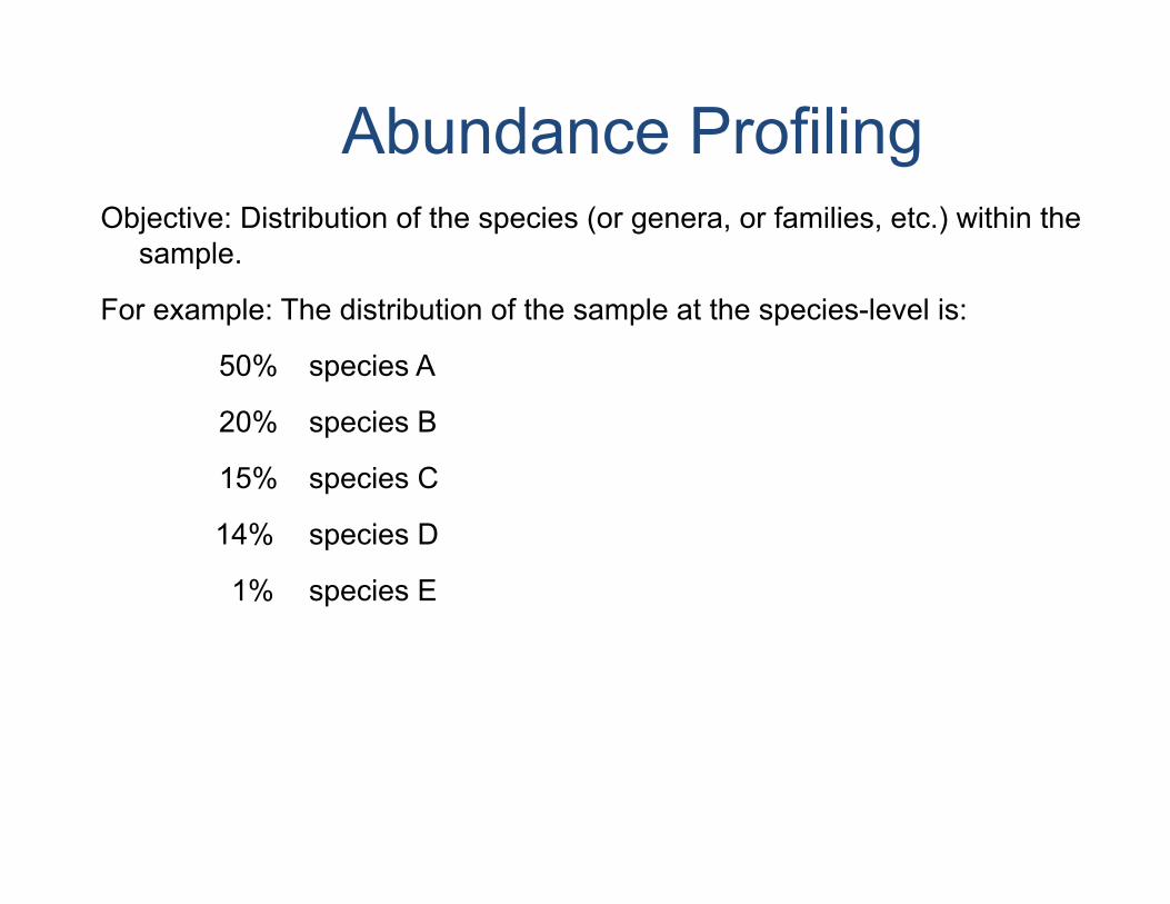
Objective: Distribution of the species (or genera, or families, etc.) within the sample.
For example: The distribution of the sample at the species-level is:
50% species A
20% species B
15% species C
14% species D
1% species E
Abundance Profiling
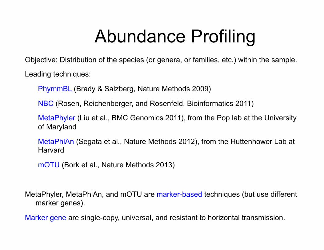
Objective: Distribution of the species (or genera, or families, etc.) within the sample.
Leading techniques:
PhymmBL (Brady & Salzberg, Nature Methods 2009)
NBC (Rosen, Reichenberger, and Rosenfeld, Bioinformatics 2011)
MetaPhyler (Liu et al., BMC Genomics 2011), from the Pop lab at the University of Maryland
MetaPhlAn (Segata et al., Nature Methods 2012), from the Huttenhower Lab at Harvard
mOTU (Bork et al., Nature Methods 2013)
MetaPhyler, MetaPhlAn, and mOTU are marker-based techniques (but use different marker genes).
Marker gene are single-copy, universal, and resistant to horizontal transmission.
Abundance Profiling
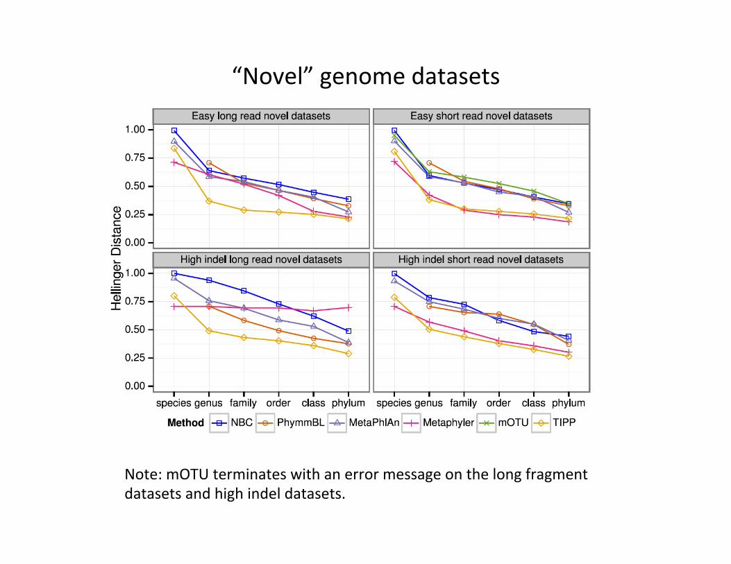
“Novel” genome datasets
Note: mOTU terminates with an error message on the long fragment datasets and high indel datasets.
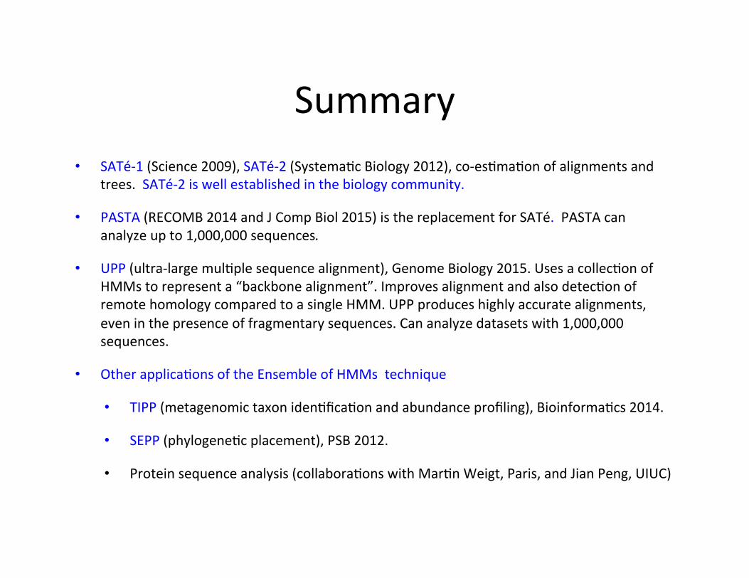
Summary • SATé-‐1 (Science 2009), SATé-‐2 (Systema,c Biology 2012), co-‐es,ma,on of alignments and
trees. SATé-‐2 is well established in the biology community.
• PASTA (RECOMB 2014 and J Comp Biol 2015) is the replacement for SATé. PASTA can analyze up to 1,000,000 sequences.
• UPP (ultra-‐large mul,ple sequence alignment), Genome Biology 2015. Uses a collec,on of HMMs to represent a “backbone alignment”. Improves alignment and also detec,on of remote homology compared to a single HMM. UPP produces highly accurate alignments, even in the presence of fragmentary sequences. Can analyze datasets with 1,000,000 sequences.
• Other applica,ons of the Ensemble of HMMs technique
• TIPP (metagenomic taxon iden,fica,on and abundance profiling), Bioinforma,cs 2014.
• SEPP (phylogene,c placement), PSB 2012.
• Protein sequence analysis (collabora,ons with Mar,n Weigt, Paris, and Jian Peng, UIUC)
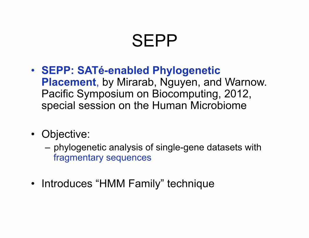
SEPP • SEPP: SATé-enabled Phylogenetic
Placement, by Mirarab, Nguyen, and Warnow. Pacific Symposium on Biocomputing, 2012, special session on the Human Microbiome
• Objective: – phylogenetic analysis of single-gene datasets with
fragmentary sequences
• Introduces “HMM Family” technique
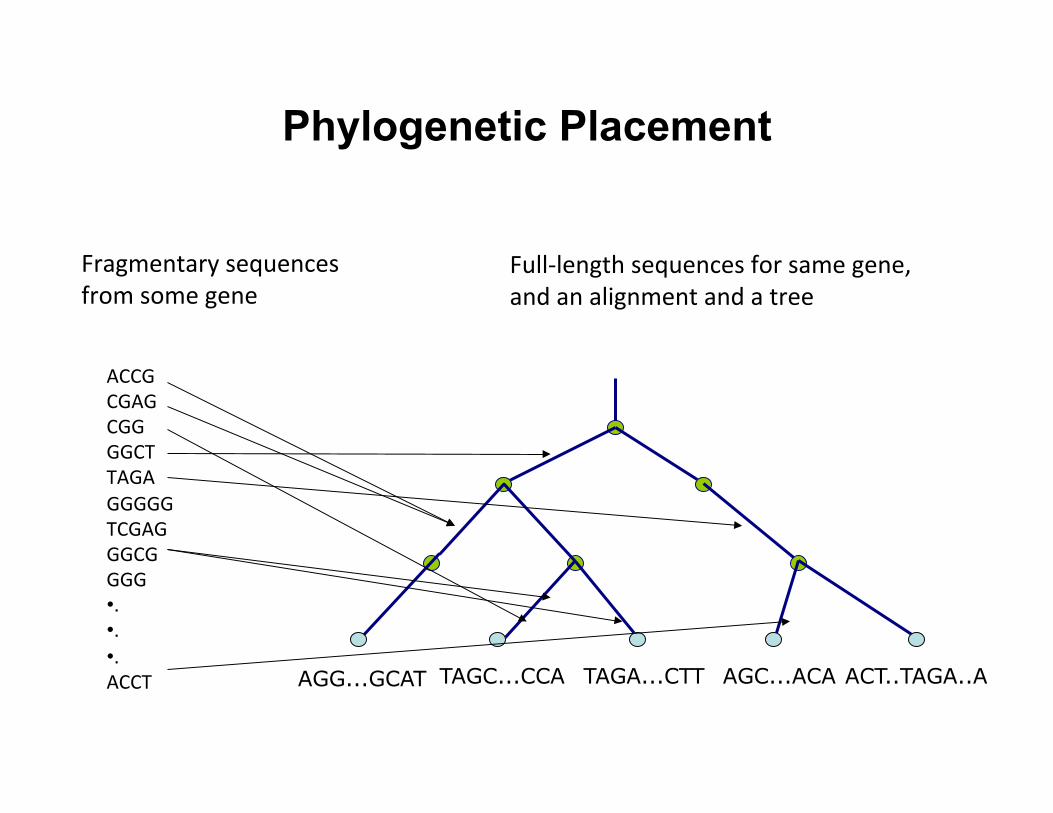
Phylogenetic Placement
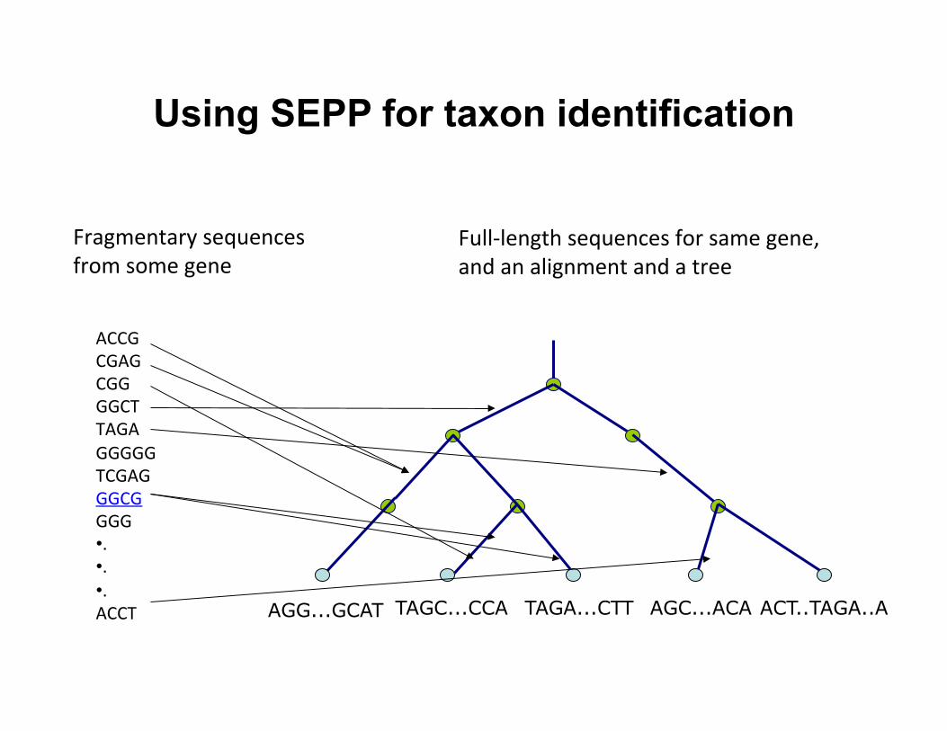
ACT..TAGA..A AGC...ACA TAGA...CTT TAGC...CCA AGG...GCAT
ACCG CGAG CGG GGCT TAGA GGGGG TCGAG GGCG GGG • . • . • . ACCT
Fragmentary sequences from some gene
Full-‐length sequences for same gene, and an alignment and a tree
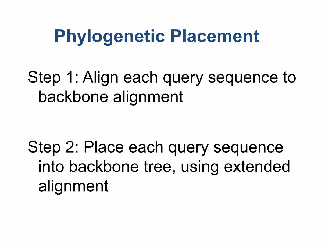
Step 1: Align each query sequence to backbone alignment
Step 2: Place each query sequence
into backbone tree, using extended alignment
Phylogenetic Placement
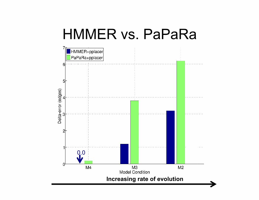
HMMER vs. PaPaRa Alignments
Increasing rate of evolution
0.0

Align Sequence
S1
S4
S2
S3
S1 = -AGGCTATCACCTGACCTCCA-AA S2 = TAG-CTATCAC--GACCGC--GCA S3 = TAG-CT-------GACCGC--GCT S4 = TAC----TCAC--GACCGACAGCT Q1 = TAAAAC
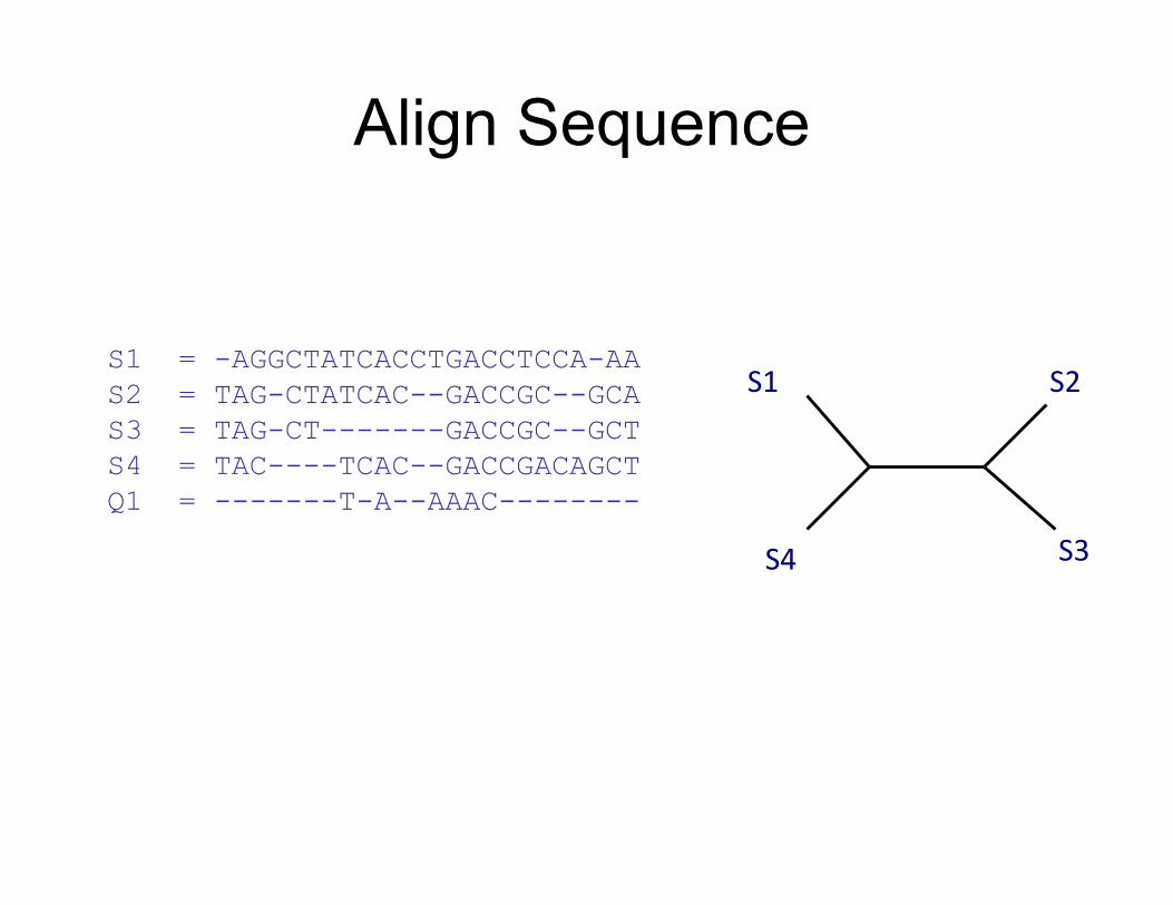
Align Sequence
S1
S4
S2
S3
S1 = -AGGCTATCACCTGACCTCCA-AA S2 = TAG-CTATCAC--GACCGC--GCA S3 = TAG-CT-------GACCGC--GCT S4 = TAC----TCAC--GACCGACAGCT Q1 = -------T-A--AAAC--------
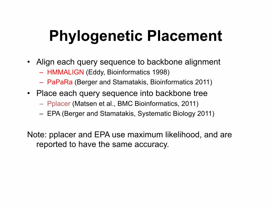
Phylogenetic Placement • Align each query sequence to backbone alignment
– HMMALIGN (Eddy, Bioinformatics 1998) – PaPaRa (Berger and Stamatakis, Bioinformatics 2011)
• Place each query sequence into backbone tree – Pplacer (Matsen et al., BMC Bioinformatics, 2011) – EPA (Berger and Stamatakis, Systematic Biology 2011)
Note: pplacer and EPA use maximum likelihood, and are reported to have the same accuracy.
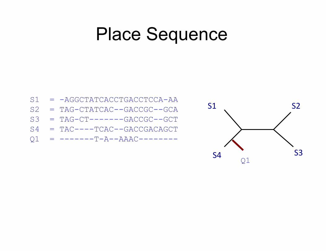
Place Sequence
S1
S4
S2
S3 Q1
S1 = -AGGCTATCACCTGACCTCCA-AA S2 = TAG-CTATCAC--GACCGC--GCA S3 = TAG-CT-------GACCGC--GCT S4 = TAC----TCAC--GACCGACAGCT Q1 = -------T-A--AAAC--------
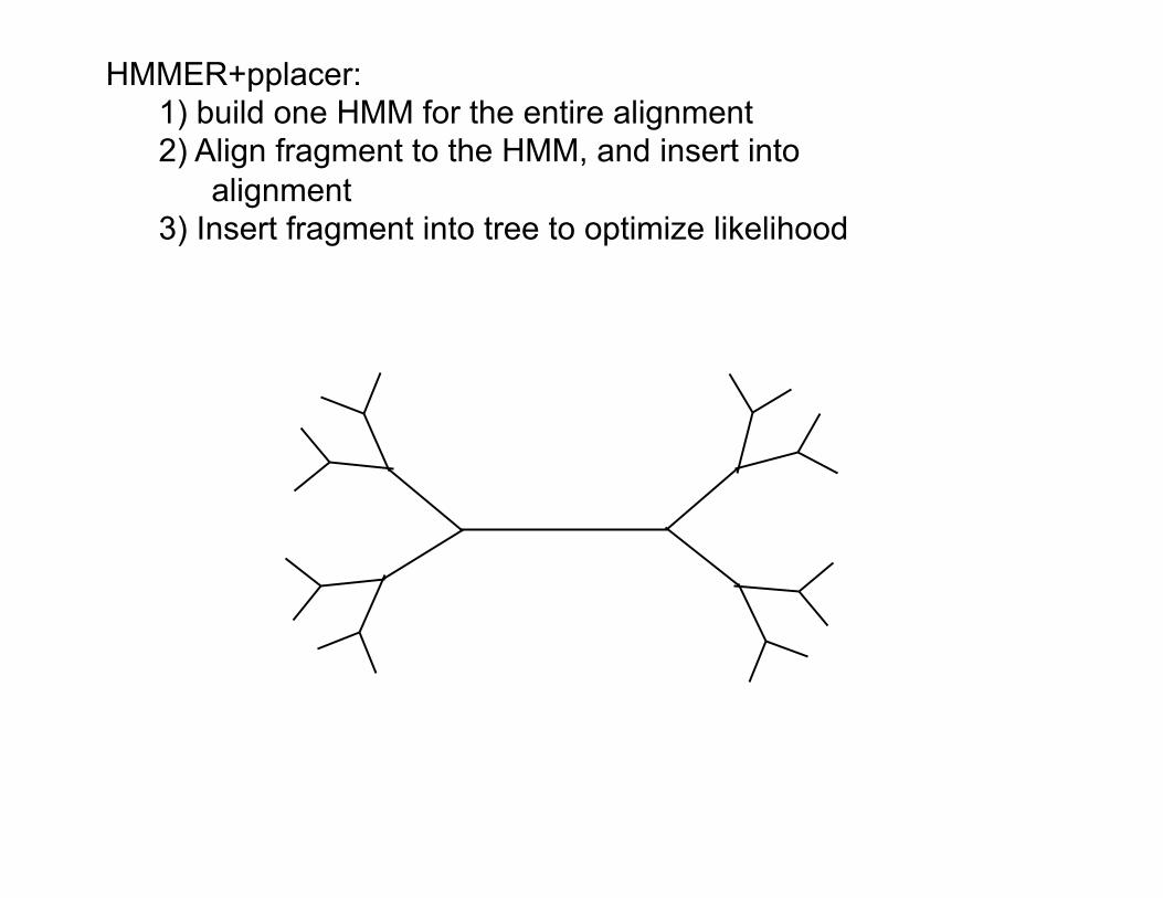
HMMER+pplacer: 1) build one HMM for the entire alignment 2) Align fragment to the HMM, and insert into
alignment 3) Insert fragment into tree to optimize likelihood
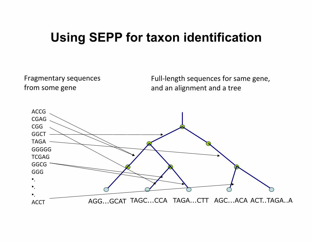
Using SEPP for taxon identification
ACT..TAGA..A AGC...ACA TAGA...CTT TAGC...CCA AGG...GCAT
ACCG CGAG CGG GGCT TAGA GGGGG TCGAG GGCG GGG • . • . • . ACCT
Fragmentary sequences from some gene
Full-‐length sequences for same gene, and an alignment and a tree
Using SEPP for taxon identification
ACT..TAGA..A AGC...ACA TAGA...CTT TAGC...CCA AGG...GCAT
ACCG CGAG CGG GGCT TAGA GGGGG TCGAG GGCG GGG • . • . • . ACCT
Fragmentary sequences from some gene
Full-‐length sequences for same gene, and an alignment and a tree
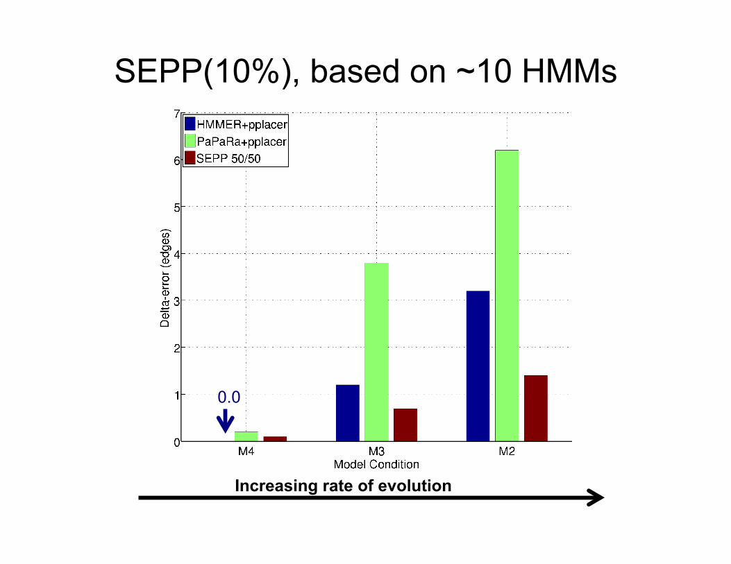
SEPP(10%), based on ~10 HMMs
0.0
0.0
Increasing rate of evolution
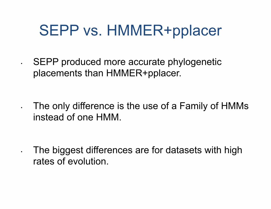
• SEPP produced more accurate phylogenetic placements than HMMER+pplacer.
• The only difference is the use of a Family of HMMs instead of one HMM.
• The biggest differences are for datasets with high rates of evolution.
SEPP vs. HMMER+pplacer
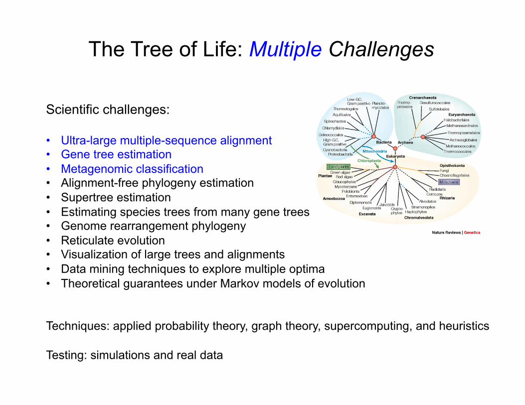
Scientific challenges: • Ultra-large multiple-sequence alignment • Gene tree estimation • Metagenomic classification • Alignment-free phylogeny estimation • Supertree estimation • Estimating species trees from many gene trees • Genome rearrangement phylogeny • Reticulate evolution • Visualization of large trees and alignments • Data mining techniques to explore multiple optima • Theoretical guarantees under Markov models of evolution
Techniques: applied probability theory, graph theory, supercomputing, and heuristics Testing: simulations and real data
The Tree of Life: Multiple Challenges
SATé-‐II running ,me profiling
�
�
�
�
�
� � � � � �� ������ � �������
�������
�����
����� �����
�
��
���
�
����
����
����
�����
�� ����� ��
� � ���� ����� �� ��
��� ������ ���
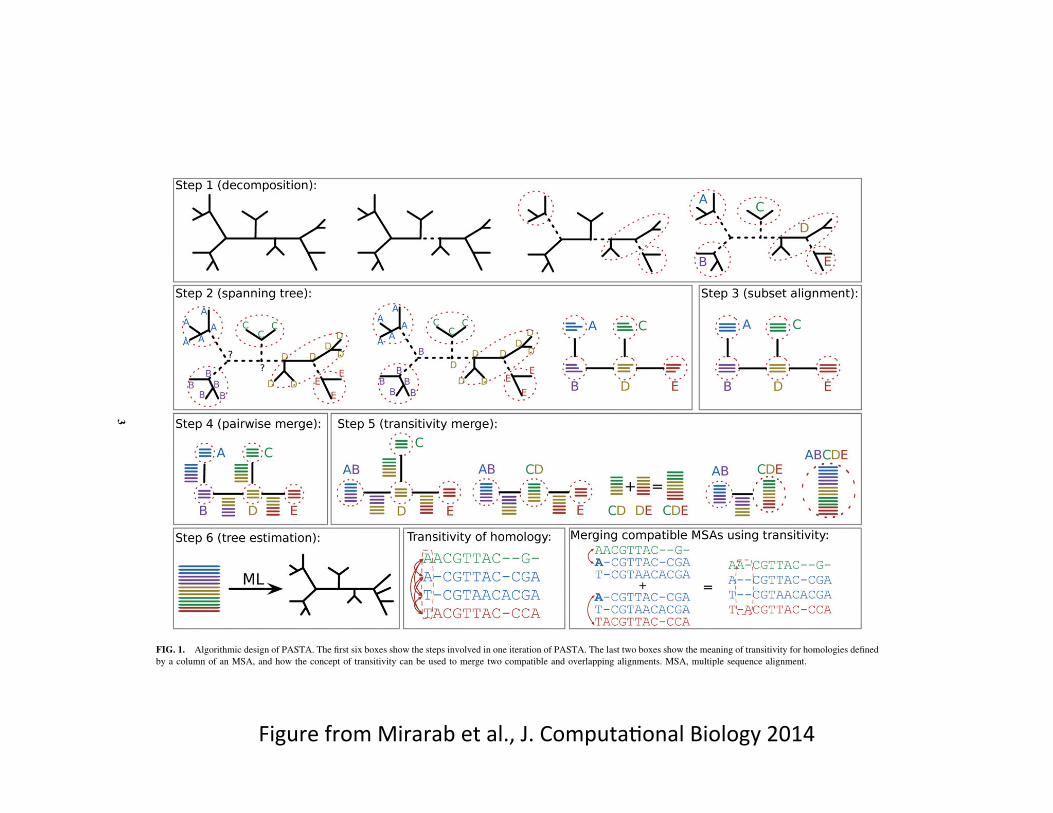
FIG. 1. Algorithmic design of PASTA. The first six boxes show the steps involved in one iteration of PASTA. The last two boxes show the meaning of transitivity for homologies definedby a column of an MSA, and how the concept of transitivity can be used to merge two compatible and overlapping alignments. MSA, multiple sequence alignment.
3
Figure from Mirarab et al., J. Computa,onal Biology 2014