unc chapel hill lin/manocha/foskey optimization problems in which a set of choices must be made in...

UNC Chapel Hill Lin/Manocha/Foskey

Optimization Problems

In which a set of choices must be made in order to arrive at an optimal (min/max) solution, subject to some constraints. (There may be several solutions to achieve an optimal value.)

Two common techniques:– Dynamic Programming (global)– Greedy Algorithms (local)


Dynamic Programming

Similar to divide-and-conquer, it breaks problems down into smaller problems that are solved recursively.

In contrast, DP is applicable when the sub-problems are not independent, i.e. when sub-problems share sub-sub-problems. It solves every sub-sub-problem just once and save the results in a table to avoid duplicated computation.


Elements of DP Algorithms

Sub-structure: decompose problem into smaller sub-problems. Express the solution of the original problem in terms of solutions for smaller problems.

Table-structure: Store the answers to the sub-problem in a table, because sub-problem solutions may be used many times.

Bottom-up computation: combine solutions on smaller sub-problems to solve larger sub-problems, and eventually arrive at a solution to the complete problem.


Applicability to Optimization Problems

Optimal sub-structure (principle of optimality): for the global problem to be solved optimally, each sub-problem should be solved optimally. This is often violated due to sub-problem overlaps. Often by being “less optimal” on one problem, we may make a big savings on another sub-problem.

Small number of sub-problems: Many NP-hard problems can be formulated as DP problems, but these formulations are not efficient, because the number of sub-problems is exponentially large. Ideally, the number of sub-problems should be at most a polynomial number.


Optimized Chain Operations

Determine the optimal sequence for performing a series of operations. (the general class of the problem is important in compiler design for code optimization & in databases for query optimization)

For example: given a series of matrices: A1…An , we can “parenthesize” this expression however we like, since matrix multiplication is associative (but not commutative).

Multiply a p x q matrix A times a q x r matrix B, the result will be a p x r matrix C. (# of columns of A must be equal to # of rows of B.)


Matrix Multiplication

In particular for 1 i p and 1 j r, C[i, j] = k = 1 to q A[i, k] B[k, j]

Observe that there are pr total entries in C and each takes O(q) time to compute, thus the total time to multiply 2 matrices is pqr.


Chain Matrix Multiplication

Given a sequence of matrices A1 A2…An , and dimensions p0 p1…pn where Ai is of dimension pi-1 x pi , determine multiplication sequence that minimizes the number of operations.

This algorithm does not perform the multiplication, it just figures out the best order in which to perform the multiplication.


Example: CMM

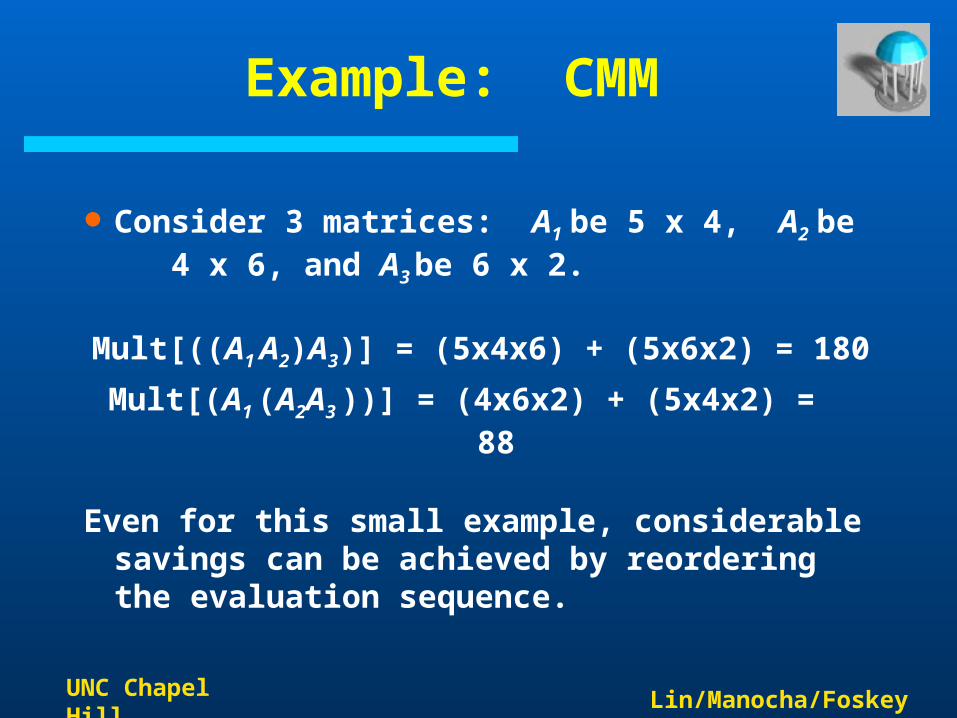
Consider 3 matrices: A1 be 5 x 4, A2 be 4 x 6, and A3 be 6 x 2.

Mult[((A1 A2)A3)] = (5x4x6) + (5x6x2) = 180

Mult[(A1 (A2A3 ))] = (4x6x2) + (5x4x2) = 88

Even for this small example, considerable savings can be achieved by reordering the evaluation sequence.


Naive Algorithm

If we have just 1 item, then there is only one way to parenthesize. If we have n items, then there are n-1 places where you could break the list with the outermost pair of parentheses, namely just after the first item, just after the 2nd item, etc. and just after the (n-1)th item.

When we split just after the kth item, we create two sub-lists to be parenthesized, one with k items and the other with n-k items. Then we consider all ways of parenthesizing these. If there are L ways to parenthesize the left sub-list, R ways to parenthesize the right sub-list, then the total possibilities is LR.


Cost of Naive Algorithm

The number of different ways of parenthesizing n items is

P(n) = 1, if n = 1

P(n) = k = 1 to n-1 P(k)P(n-k), if n 2

This is related to Catalan numbers (which in turn is related to the number of different binary trees on n nodes). Specifically P(n) = C(n-1).

C(n) = (1/(n+1)) C(2n, n) (4n / n3/2)

where C(2n, n) stands for the number of various ways to choose n items out of 2n items total.


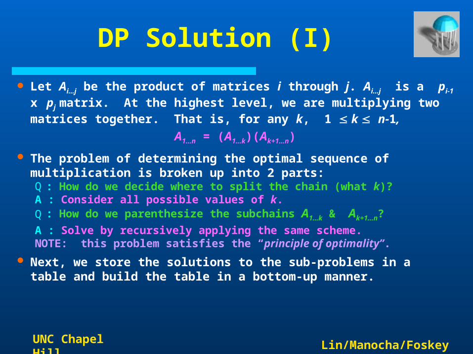
DP Solution (I)

Let Ai…j be the product of matrices i through j. Ai…j is a pi-1 x pj matrix. At the highest level, we are multiplying two matrices together. That is, for any k, 1 k n-1,

A1…n = (A1…k)(Ak+1…n)

The problem of determining the optimal sequence of multiplication is broken up into 2 parts: Q : How do we decide where to split the chain (what k)?A : Consider all possible values of k.Q : How do we parenthesize the subchains A1…k & Ak+1…n?

A : Solve by recursively applying the same scheme.NOTE: this problem satisfies the “principle of optimality”.

Next, we store the solutions to the sub-problems in a table and build the table in a bottom-up manner.


DP Solution (II)

For 1 i j n, let m[i, j] denote the minimum number of multiplications needed to compute Ai…j .

Example: Minimum number of multiplies for A3…7

98

]7,3[

7654321 AAAAAAAAAm

In terms of pi , the product A3…7 has

dimensions ____.


DP Solution (III)

The optimal cost can be described be as follows:– i = j the sequence contains only 1 matrix, so m[i, j] = 0.– i < j This can be split by considering each k, i k < j,

as Ai…k (pi-1 x pk ) times Ak+1…j (pk x pj).

This suggests the following recursive rule for computing m[i, j]:

m[i, i] = 0

m[i, j] = mini k < j (m[i, k] + m[k+1, j] + pi-1pkpj ) for i < j


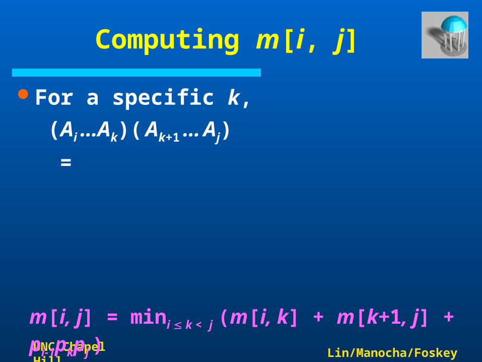
Computing m[i, j]

For a specific k,

(Ai …Ak)( Ak+1 … Aj)

=

m[i, j] = mini k < j (m[i, k] + m[k+1, j] + pi-1pkpj )


Computing m[i, j]

For a specific k,


= Ai…k( Ak+1 … Aj) (m[i, k] mults)



Computing m[i, j]

For a specific k,



= Ai…k Ak+1…j (m[k+1, j] mults)



Computing m[i, j]

For a specific k,




= Ai…j (pi-1 pk pj mults)



Computing m[i, j]

For a specific k,




= Ai…j (pi-1 pk pj mults)

For solution, evaluate for all k and take minimum.



Matrix-Chain-Order(p)

1. n length[p] - 12. for i 1 to n // initialization: O(n) time3. do m[i, i] 04. for L 2 to n // L = length of sub-chain5. do for i 1 to n - L+1 6. do j i + L - 1 7. m[i, j] 8. for k i to j - 1 9. do q m[i, k] + m[k+1, j] + pi-1 pk pj

10. if q < m[i, j]11. then m[i, j] q12. s[i, j] k13. return m and s


Analysis

The array s[i, j] is used to extract the actual sequence (see next).

There are 3 nested loops and each can iterate at most n times, so the total running time is (n3).


Extracting Optimum Sequence

Leave a split marker indicating where the best split is (i.e. the value of k leading to minimum values of m[i, j]). We maintain a parallel array s[i, j] in which we store the value of k providing the optimal split.

If s[i, j] = k, the best way to multiply the sub-chain Ai…j is to first multiply the sub-chain Ai…k and then the sub-

chain Ak+1…j , and finally multiply them together. Intuitively s[i, j] tells us what multiplication to perform last. We only need to store s[i, j] if we have at least 2 matrices & j > i.


Mult (A, i, j)

1. if (j > i)

2. then k = s[i, j]

3. X = Mult(A, i, k) // X = A[i]...A[k]

4. Y = Mult(A, k+1, j) // Y = A[k+1]...A[j]

5. return X*Y // Multiply X*Y

6. else return A[i] // Return ith matrix


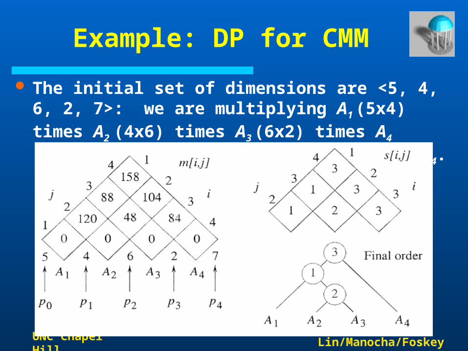
Example: DP for CMM

The initial set of dimensions are <5, 4, 6, 2, 7>: we are multiplying A1 (5x4) times A2 (4x6) times A3 (6x2) times A4 (2x7). Optimal sequence is (A1 (A2A3 )) A4.


Finding a Recursive Solution

Figure out the “top-level” choice you have to make (e.g., where to split the list of matrices)

List the options for that decisionEach option should require smaller

sub-problems to be solvedRecursive function is the minimum

(or max) over all the options


unc chapel hill lin/manocha/foskey optimization problems in which a set of choices must be made in...

Documents

number of sub problems

smaller subproblems

larger sub problems

subproblem solutions

subproblem overlaps

small number of subproblems

smaller problems

dp problems