uncertainty and competition in the adoption of
TRANSCRIPT

1
Uncertainty and Competition in the Adoption of
Complementary Technologies
Alcino F. Azevedo1,* and Dean A. Paxson**
*Hull University Business School
Cottingham Road, Hull HU6 7RX, UK
**Manchester Business School
Booth Street West, Manchester M15 6PB, UK
Abstract
We study the combined effects of uncertainty, competition and “technological complementarity” on
firms’ investment behaviour in a leader/follower pre-emption investment game. Our results
contradict the conventional wisdom which says that “when a production process requires two
extremely complementary inputs, a firm should upgrade (or replace) them simultaneously”. We
found that when competition and uncertainty are considered, this is very unlikely to be the case for
the leader and mixed strategies are possible for the follower. Some of the illustrated results show
nonlinear and complex investment criteria and significant differences between the leader’s and the
follower’s investment behavior.
JEL Classification: D81, D92, O33.
Key Words: Real Options, Uncertainty, Pre-emption, Duopoly Games, Technological
Complementarity.
1 Corresponding author: Tel.: +44(0)1482463107, Fax: +44(0)1482463484, [email protected].

2
1. Introduction
Since the pioneering work of Smets (1993), the effect of uncertainty and competition on investment
behavior in a duopoly has been extensively studied in the real options literature2, but the influence
of the degree of complementarity between the inputs of an investment on firms’ investment
decisions has been neglected. However, firms often use inputs whose qualities are complements,
such as computer and modem, equipment and structure, train and track, and transmitter and
receiver. In such cases, investment decisions on upgrades or replacements must consider the degree
of complementarity between investments. In this paper, “complementarity” exists if the adoption of
one technology increases the marginal or incremental return to other technology in terms of cost
savings. More generally, in the context of industrial organization, complementarity exists if the
implementation of one practice increases the marginal return to other practice (Carree et al., 2010).
When the implementation of a technology/practice decreases the marginal return to the other
technology/practice, there is “substitutability” (or subadditivity)3.
The concept of complementarity has been used to study economic decisions in many contexts. In
the context of a country, it is used to set innovation policies, for instance, the optimization of the
balance between technology imports and in-house R&D (Braga and Wilmore, 1991) and (Cassiman
and Veugelers, 2004), the allocation of financial resources to industries (Mohnen and Roller, 2000),
to enhance innovation and/or to favor clustering (Anderson and Schmittlein, 1984), and to define
production policies, for instance, the coordination between product and process innovation
(Miravete and Pernías, 1998).
R&D is an area where the concept of complementarity plays an important role, since when planning
their R&D activities, firms make strategic decisions regarding the degree of complementarity
(sometimes called compatibility) between the new products they aim to launch in the future and the
complement products that are already available in the market and those they conjecture will be
launched by their opponents in the future, in the sense that the diffusion of an innovation depends,
to some extent, on the diffusion of complement innovations which amplify its value4. It has been
2 Dixit and Pindyck (1994), chapter 9, Grenadier (1996), Lambrecht and Perraudin (1997), Huisman (2001),
Weeds (2002) and Paxson and Pinto (2005), Pawlina and Kort (2006) address such problems. 3 See Carree et al. (2010) for further details on this issue.
4 Note that, in R&D contexts, firms who do not have a dominant market position and want to growth quickly
tend to guide their R&D efforts in order to launch new products that are compatible with those from their
opponents who have a dominant market positions; firms who have dominant market positions tend to guide
their R&D efforts in order to launch new products that are, as much as possible, not complements (compatible) with rivals. An example of the later strategy is the nine-year battle between the European Union
(EU) commission and Microsoft that culminated in October 2007 with a fine of €497 million due to its
supposed misconduct in developing software that does not allow open-source software developers access to

3
also argued that the pace of modernization of an industry is quite often influenced by the degree of
technological complementarity between the new technologies adopted in that industry5.
The concept of complementarity between economic activities (sometimes referred in the literature
as synergy) plays also an important role in mergers and acquisitions since these are guided by the
level of complementarity between firms’ businesses processes, technologies, IT applications,
clients, geographic location, etc. The merger between Air France and KLM and the acquisition of
Abbey by Santander, in 2004, are two good examples of the importance of the complementary
concept. In the former case, both firms justified the merger on the strong complementarity between
their businesses in terms of the optimization of networks based on two powerful hubs, the
possibility of using a more effective redeployment of passenger and cargo activities and expanding
the offer of aircraft maintenance services, and the existence of cost savings in purchasing, sales
distribution and IT applications; in the latter, Santander justified the acquisition of Abbey based on
similar arguments and emphasizing the fact that, apart from other important business
complementarities, the existence of a strong complementarity between the two banks IT
applications was very important in the outcome of its decision given that it facilitates the
integration of the two banks businesses6.
Examples of relevant contributions to the literature around the concept of “complementarity” and its
use in economic analyses are Milgrom and Roberts (1990, 1995), who use the theories of
supermodular optimization and games as a framework for the analysis of systems marked by
complementarity; Milgrom and Roberts (1994), who study the Japanese economy between 1940
and 1995 to interpret the characteristic features of Japanese economic organization in terms of the
complementarity between some of the most important elements of its economic structure; and
Colombo and Mosconi (1995), who examine the diffusion of flexible automation production and
design/engineering technologies in the Italian metalworking industry, giving particular attention to
the role of the technological complementarity and the learning effects associated with the
experience of previously available technologies.
inter-operability information for work-group servers used by businesses and other big organizations (see Etro
(2007), p. 221, and Financial Times, October 23, 2007, p. 1). 5 Smith and Weil (2005) investigated how changes in retailing and manufacturing industries, together,
affected the diffusion of new information technologies in the U.S. apparel industry between 1988 and 1992,
and suggest that there is a significant effect of the complementarity between new technologies on the pace of
modernization of interlinked industries. 6 For detailed information about this and other merger and acquisitions in EU see the “European Foundation
for the Improvement of Living and Working Conditions” website: http://www.eurofound.europa.eu/.

4
Conventional wisdom says that “when a production process requires two extremely complementary
inputs, a firm should upgrade (or replace) them simultaneously”, i.e., when raising the quality of
one input it should upgrade its complements at the same time (Javanovic and Stolyarov, 2000, p.
15). From Milgrom and Robert (1990, 1995) models, we infer that it is relatively unprofitable to
adopt only one part of the modern manufacturing strategy. In Milgrom and Roberts (1990, p. 524),
it is suggested that “we should not see an extended period of time during which there are substantial
volumes of both highly flexible and highly specialized (i.e., non-complementary) equipment being
used side-by-side”. Cho and McCardle (2009) show that the economic dependence that inherently
defines cost relationships inside the firm can significantly influence the timing of adoption, by
expediting or delaying the adoption of an improved technology.
However, the conclusions above have been made for contexts where uncertainty and competition
are ignored. We study the effect of the complementarity between two technologies on their optimal
time of adoption, considering competition between (two) firms and uncertainty about revenues and
investment costs. Smith (2005) studies a similar problem but neglects competition.
Our initial intuition is that when uncertainty or drift differences about the investment cost of the
technologies is considered, the conventional wisdom stated above may not hold, since due to
technological progress the cost of a technology can decline rapidly. When firms anticipate that the
cost of technologies may not fall at the same rate, it may pay to adopt first the technology whose
cost is falling more slowly and wait to adopt the technologies whose cost is falling more rapidly.
The manufacturing industry is by nature a sector where the concept of technological (or
performance) complementarity applies to and where some of our results can be empirically tested.
Azevedo and Paxson (2008) use empirical evidence from two firms from the Portuguese textile
industry, whose production activities (units) have strong efficiency complementarity, to show
some of the results highlighted in this research.
In our model, the word “complementarity” between the two technologies means the degree to which
two technologies are better off when operating together rather than operating alone; 12 in
inequality 12 1 2 , is the parameter that represents the degree of complementarity between
the two technologies, where, 1 and 2 are defined as the proportion of the firm’s revenues that are
expected to be saved if tech 1 and tech 2, respectively, are adopted alone (i.e., firms operate with
one technology, tech 1 or tech 2), and 12 is the proportion of the firm’s revenues that are expected

5
to be saved if both technologies are adopted together (i.e., firms operate with the two technologies
at the same time).
There are econometric techniques to test/estimate complementarity between industrial organization
practices, namely the “adoption” or “correlation” approach and the “production function” approach
(Carree et al., 2010). Detailed descriptions of the techniques and empirical examples of the concept
of “complementarity” can be found in Arora and Gambardella (1990), who suggest a test for
complementarity, and Arora (1996), Athey and Stern (1998), and Miravete and Pernías (1998,
2010).
We use a real options methodology to derive, for a duopoly market with a first-mover advantage,
analytical expressions for the value functions of the leader and the follower and their respective
investment threshold values. We assume that the market is composed of two idle firms7; at the
beginning of the investment game there are two new (complementary) technologies available, tech
1 and tech 2; firms are allowed to invest twice; firms’ cost savings are a proportion of the firms’
revenues; and both the revenues and the cost of each technology are uncertain, following
independent, and possible correlated, geometric Brownian motion (gBm) processes.
The rest of this paper is organized as follows. In section 2, we outline the model assumptions and
define the duopoly investment game. In section 3, we derive the firms’ value functions and their
investment threshold values. Section 4 presents the results. Section 5 concludes and offers some
guidelines for possible extensions of this research.
7 In this paper, an idle firm means a firm which is inactive or that it is active but operating without the most
recent technology. For instance, a firm operating with an old rail train with old tracks is idle in not yet
adopting high-speed trains and new tracks, if available.

6
2. The Investment Game
In Figure 1 we represent the investment game using an extensive-form representation8.
Time, (continuous-time)
i
tech1(2) wait
tech 12 j j i
tech 1(2) wait tech 12 tech 1(2) wait tech 12 tech 1(2) wait
1,1( )LF
1,0
( )LF 12,12
( )SM
LF
12,1(2)( )LF
12,0( )LF
12,0( )LF
1,0( )LF
0,0( )LF
1,1
( )FF 0,1
( )FF 12,12
( )SM
FF 1(2),12
( )FF 0,12
( )FF 0,12
( )FF 0,1
( )FF 0,0
( )FF
(S1) (S2) j i i
tech2(1) wait
j j tech2(1) wait tech 12 tech 1(2) wait
tech2(1) wait tech2(1) wait
Firm i 1 2,1 2
( )SQ
LF
12,1( )LF
1,12
( )LF 1,1
( )LF 12,1 2
( )SQ
LF
12,1(2)
( )LF 12,0
( )LF 0,1
( )LF 0,0
( )LF
Firm j 1 2,1 2
( )SQ
FF
1,12( )FF
12,1
( )FF 1,1
( )FF 1 2,12
( )SQ
FF
1(2),12
( )FF 0,12
( )FF 1,0
( )FF 0,0
( )FF
(S3)
Figure 1 - Extensive-form Representation of a Continuous-time Real Option Game (CTROG)
with Two Firms and Two Complementary Technologies.
Regarding the notation above, ,
( )k kiF , represents the firm’s value function for a particular
investment game scenario, where ,i L F , with “L” and “F” meaning “leader” and “follower”,
respectively, 1,2,12k , with “1”, “2” and “12” representing, respectively, the case where the
firm operates with “technology 1 alone”, “technology 2 alone” or with “technology 1 and 2 at the
same time”; k is the ratio “market revenue” ( X ) over the cost ( I ) of technology k, /k kX I 9;
the superscripts “SM” and “SQ” on some of the value functions mean “simultaneous investment”
8 For a detailed description of this type of game representation see Gibbons (1992). For an extensive literature
review on real option games, with detailed descriptions about the game theory concepts and how to combine
them with the real option framework, see Azevedo and Paxson (2010). 9 In the game-tree we drop the subscript k for simplicity of notation.

7
(i.e., investment on tech 1 and tech 2 at the same time) and “sequential investment” (i.e., investment
on tech 1 and tech 2 sequentially), respectively10
.
In section 3 we derive the firms’ value functions and investment thresholds for the scenarios
identified in Figure 1 as (S1), (S2) and (S3). Below we characterize these investment scenarios.
Scenario 1 (S1): firm i adopts first tech 1(2) and becomes the leader, firm j adopts later tech 1(2),
and becomes the follower. The payoffs for firm i and j are given, respectively, by 1,1
( )LF
and1,1
( )FF . Scenario 2 (S2): firm i adopts first tech 1 and tech 2 (tech 12) simultaneously, and
firm j does the same later. Firm i becomes the leader and firm j the follower and their payoffs are,
respectively, 12,12
( )SM
LF and 12,12
( )SM
FF . Scenario 3 (S3): in the first two rounds of the game, firms i
and j adopt tech 1 or tech 2 (tech 1(2)). Firm i adopts first (first round) and becomes the leader, firm
j adopts second (second round) and becomes the follower. Then, at the third and fourth rounds of
the game, both firms adopt the remaining technology available tech 2(1), again, one after the other,
firm i first and firm j second, and the firms’ payoffs are given by 12,12
( )SQ
LF and 12,12
( )SQ
FF ,
respectively for firm i and j.
In the next section we derive analytical expressions for the firms’ value functions marked in Figure
1 with an ellipse (S1, S2 and S3). Figure 2 below is an illustration of the investment scenarios
denoted in Figure 1 by (S1) and (S3), i.e., timelines for the investment thresholds of the leader and
the follower, for the cases where the two technologies are adopted sequentially, first tech 1(2), (S1
in the game-tree), and then tech 2(1), (S3 in the game-tree).
Time 0 *
1L
*
1F
*
1 2L
*
1 2F
Figure 2 – Firms’ Investment Thresholds when the Two Technologies
are Adopted Sequentially.
10
For instance, 1,1
( )LF and 1,1
( )FF represent, respectively, the value functions of the leader (L) and the
follower (F) for the scenario where both firms operate with tech 1; 12,12
( )SM
LF and 12,12
( )SM
FF represent,
respectively, the value function of the leader and the follower for the scenario where both firms adopted tech
1 and tech 2 simultaneously; 1 2,1 2
( )SQ
LF
and 1 2,1 2
( )SQ
FF
represent, respectively, the value function of the leader
and the follower for the scenario where both firms adopted tech 1 and tech 2 sequentially, first tech 1 and then
tech 2. Similar rationale applies to the notation used for the rest of the value functions in the game-tree.

8
*
1L represents the leader’s investment threshold to adopt tech 1, given that none of the technologies
have been adopted; *
1F denotes the follower’s investment threshold to adopt tech 1, when the leader
is operating with tech 1 and the follower is not yet in the market; *
1 2L is the leader’s investment
threshold to adopt tech 2 given that tech 1 is in place; and *
1 2F is the follower’s investment
threshold to adopt tech 2 given that it has adopted tech 1 and the leader is already operating with
both tech 1 and tech 2.
Figure 3 represents the firms’ investment threshold for the scenario where at the beginning of the
investment game none of the technologies have been adopted and the two firms, one after the other,
adopt the two technologies simultaneously (S2 in the game-tree); *
12L and
*
12F represent,
respectively, the leader’s and the follower’s investment thresholds.
Time 0 *
12L *
12F
Figure 3 – Firms’ Investment Thresholds when the Two Technologies
are Adopted Simultaneously.
Table 1 is a summary of the investment thresholds.
* The mathematical expressions for the firms’ investment threshold to adopt tech 1 and tech 2 alone are exactly the same, only the subscripts (1, 2)
change.
** In the derivation of these expressions we assumed firms adopt tech 1 first and afterwards tech 2. However, nothing would change if we had assumed
the other way round, apart from reversing the subscripts (1, 2).
Note: the terms S1, S2 and S3 above represent the investment game scenarios identified in the game-tree, p. 6.
Table 1 - Investment Thresholds for the Scenarios where Firms Adopt the Two
Technologies, Sequentially and Simultaneously.
Firms’ Investment
Trigger Values
The Adoption*
of Tech 1 or Tech 2 alone
Sequential Adoption** (tech 1/tech 2)
Simultaneous Adoption
(tech 1 + tech 2)
Leader
*
1L
Equation (28)
(S1)
*
2L
Equation (28)
(S1)
*
1 2L
Equation (16)
(S3)
*
12L
Equation (32)
(S2)
Follower
*
1F
Equation (24)
(S1)
*
2F
Equation (24)
(S1)
*
1 2F
Equation (11)
(S3)
*
12F
Equation (30)
(S2)
Due to the high number of the investment scenarios available, to avoid unnecessary complexity and
without any lost of insight, we focus our derivation and analyses only on the scenarios marked in
Figure 1 with an ellipse, i.e., (S1), (S2) and (S3). In addition, we assume that firms are not allowed
to invest at the same time, i.e., if that occurs one of the firms will become the leader by flipping a

9
coin. Nevertheless, these constrains in our analyses do not impose any lost of insight because, the
framework and the nature of the methodology used to derive the firms’ value functions and
respective investment thresholds for scenarios (S1), (S2) and (S3) are informative enough to infer
the results for the other investment scenarios. Additional information about another investment
game scenario is provided in the Appendix A, section 5.
2.1 The Pre-emption Game
In games of timing the adoption of new technologies, the potential advantage of being the first to
adopt may introduce an incentive for pre-empting the rival, speeding up the first adoption.
Fudenberg and Tirole (1985) studied the adoption of a new technology and illustrate the effects of
pre-emption in games of timing. We use their concept of pre-emption to derive the firms’ value
functions and investment thresholds.
3. The Model
In a risk-neutral world, at the beginning of the investment game, there are two new
(complementary) technologies available, tech 1 and tech 2, and two idle firms, i and j, which are
considering the adoption of the two technologies, one after the other or both simultaneously
depending on which one of these choices is the best.
The firms’ cost savings flow is given by the following expression:
( )i jk k kX t ds
(1)
where, k represents the proportion of a firm’s revenues that is expected to be saved through the
adoption of technology k, with 0,1,2,12k , where 0 means that firm is not yet active and 1, 2
and 12 mean that firm operates with tech 1 only, tech 2 only or tech 1 and tech 2 at the same time,
respectively; ( )X t is the total market revenue flow; i jk kds
is a competition (deterministic) factor
that ensures a first-mover market share (revenue) advantage, with , ,i j L F , where L means
“leader” and F “follower”, and represents the “proportion of the total market revenues” 11
that is
held by each firm for each investment scenario. The relationship between these competition factors
is governed by inequality (2).
11
Suppose that by adopting a new technology a firm can get a 10% reduction in its operating costs per unit.
Hence, within a certain production range, the more it produces/sales the more it saves due to the adoption of
the technology.

10
The intuition used to justify the first-mover “market share advantage” is similar to that used by
Dixit and Pindyck (1994), following Smets (1993). Implicitly we also assume that firms are
symmetric in their ability to operate with the new technologies and that spillover information is not
allowed, i.e., firms’ “first-mover market share advantage” holds forever. In addition, the exit
strategy is no allowed.
Consequently, for the leader, inequality (2) holds:
12 0 1 0 2 0 12 1 12 12 1 1 2 2L F L F L F L F L F L F L Fds ds ds ds ds ds ds
(2)
As in a duopoly, the market share of the follower is a complement of the leader’s, i.e.,
1F L L Fk k k kds ds , with 1,2,12k , inequality (3) holds for the follower:
1 1 2 2 12 12 1 12 0 12 0 1 0 2F L F L F L F L F L F L F Lds ds ds ds ds ds ds
(3)
The economic interpretation for inequality (2) is the following: for firm L (the leader), the best
investment scenario, in terms of market share, is when it is active with either tech 1 or tech 2, alone,
or with both technologies at the same time, and its rival firm F (the follower), is inactive
12 0 1 0 2 0L F L F L Fds ds ds
12; its second best investment scenario is when it adopts both technologies
first, and its rival adopts later only tech 1 ( 12 1L Fds ); its third best investment scenario is when both
firms adopt both technologies but the leader does so earlier ( 12 12L Fds ); its fourth best investment
scenario is when both firms adopt one technology, tech 1 or tech 2, but the leader does so earlier
1 1 2 2L F L Fds ds
. It is implicitly assumed that ( 0 0 0 0 0L F L F
ds ds ), i.e., when both firms are
inactive their payoff is zero13
. Similar rational applies to the follower’s inequality. A practical
illustration about how these factors work in practice and their influence on the determination of the
firms’ value functions and the equilibrium of the game is given in Appendix B, sections 3 and 4.
12
We assume that tech 1 and tech 2 are symmetric. Hence, 1 0 2 0L F L F
ds ds ; 2 2 1 1L F L F
ds ds , i.e., the leader’s
first-mover market share advantage is the same regardless of the technology chosen. Our framework allows
however the use of different assumptions in this regard. 13
Note that, by assumption, the leader is the firm who adopts first. Hence, the scenario in which the follower
is active and the leader is inactive is not considered.

11
In addition, we assume that total market revenues, ( )X t , follow a geometric Brownian motion
given by the following equation:
X X XdX Xdt Xdz (4)
where, X is the trend rate of growth of market revenues, X is the volatility of the market
revenues and Xdz is the increment of a standard Wiener process.
We consider that tech 1 alone provides a net cost savings, 1S , that is a fraction, 1 , of the firm’s
market revenues, i jk kX ds
:
1 1 i jk kS X ds
(5)
Since the firms’ cost savings are proportional to revenues and revenues follow a gBm process, so
firms’ cost savings also follows a gBm process.
Similarly, the use of tech 2 alone provides a cost savings equal to:
2 2 i jk kS X ds
(6)
And the simultaneous use of both technologies yields cost savings equal to:
12 i jk kS X ds
(7)
The technological complementarity between the two technologies is given by the following
inequality:
12 1 2 (8)
In practice, 1 and 2 are technology/product-specific, independent, and not necessarily correlated.
For instance, technologies used to produce multi products/services may have different degrees of
complementarity regarding each of the product/service. This fact explains why firms with huge

12
fixed assets, manufacturing sector for instance, tend to guide their R&D policies to take advantage
of the assets (technologies) in place.
Furthermore, we assume that the costs of adopting tech 1 and tech 2, respectively, 1I and 2I , follow
gBm processes as well, given by:
1 1 11 1 1I I IdI I dt I dz (9)
and
2 2 22 2 2I I IdI I dt I dz (10)
where, 1I
and 2I are the trend rates of growth of the cost of tech 1 and tech 2, respectively;
1I
and 2I are the volatility of the cost of tech 1 and tech 2, respectively; and
1Idz and
2Idz are the
increments of the standard Wiener processes for the costs tech 1 and tech 2, respectively. For
convergence reasons 0X kr holds.
In some cases, correlation between “revenues” and “cost of tech 1(2)” and between “cost of tech 1”
and “cost of tech 2” are possible. This fact is considered in our model, Equations A2, A6, A9, 17,
18 and 22.
3.1 Technology 1 is in place
3.1.1 The Follower’s Value Function
In this section we derive the follower’s value function, 1 2,1 2 2( )SQ
FF
, and investment threshold,
*
1 2F , to adopt tech 2 assuming that tech 1 is in place. Below are the results. See Appendix A,
section 1, pp. 27-30, for a detailed derivation.
The follower’s investment threshold, *
1 2F , is given by equation (11):
2* 11 2
1 12 1 12 12 1 1 12
( )
1 ( )F
F L F L
X Ir
ds ds
(11)
With 1 2A given by equation (12):

13
1
2
*
1 2 12 1 12 12 1 1 12
1 2
1
( )
1
F F L F L
X I
ds dsA
r
(12)
And the follower’s value function is given by equation (13):
1
1 2,1 2
1 1 12 *21 2 2 2 1 2*
1 2
2
12 12 12 * *
2 2 1 2
( )
F L
F
F
F L
F F
XSQ
F
X
X dsA I
rF
X dsI
r
(13)
Scenario (S3) in the game-tree, p. 6.
Equation (13) tells us that for the follower, before *
1 2F is reached, its value, when it adopts the two
technologies sequentially, is given by the value of operating with tech 1 forever, 1 1 12F L
X
X ds
r
, plus
its option to adopt tech 2, 1
21 2 2*
1 2
F
A I
; as soon as *
1 2F is reached and it adopts tech 2, its value
is equal to the present value, in perpetuity, of the cost savings obtained from operating with both
technologies from *
1 2F until infinity, 12 12 12 *
2
F L
F
X
X dsI
r
.
3.1.2 The Leader’s Value Function
Assuming that both firms are operating with tech 1 and that the follower will adopt tech 2 at *
1 2F
(derived above), the leader’s value function is described by the following expression:
2 22
2
( )*
12 12 1 2 12 12 120
LF L
L F L L FF
T T rTr r
t TE X ds e d I e X ds e d
(14)
where, the first integral represents the leader’s cost savings in the period where it operates with the
two technologies and the follower operates with tech 1; the second integral represents the leader’s
cost savings for the period where both firms are operating with the two technologies, tech 1 and
tech 2; *
2LI is the cost of tech 2 at the leader’s adoption time.

14
Applying the methodology used in Dixit and Pindyck (1994), pp. 309-315, we get the following
expression for the leader’s value function:
1
1 2,1 2
12 12 1 *1 212 12 12 12 1 2 2 1 2*
1 1 2
2
12 12 12 * *
2 2 1 2
1
( )
L F
L F L F F
F
L F
L F
XSQ
L
X
X dsds ds I
rF
X dsI
r
(15)
Scenario (S3) in the game-tree, p. 6.
Expression 12 12 1L F
X
X ds
r
corresponds to the leader’s total payoff if it operates alone with the two
technologies forever; 1
1 212 12 12 12 1 2*
1 1 21 L F L F
F
ds ds I
is negative, given that 12 12 12 1 0
L F L Fds ds
(inequality 2, p. 10), and corresponds to the correction factor that incorporates the fact that in the
future if *
1 2F is reached the follower will adopt tech 2 and the leader’s profits will be reduced.
12 12 12 *
2
L F
L
X
X dsI
r
is the leader’s total payoff if it operates with the follower, both with the two
technologies from *
1 2F until infinity.
There is no closed-form solution for the leader’s investment threshold value. However, numerical
methods can be used to solve to equation (16) for *
1 2L . Equation (16) is derived by equalizing the
value functions of the leader and the follower, for *
2 1 2F .
1 1
12 12 1 1 1 12* *1 2 22 12 12 12 12 1 2 1 12 2* *
1 1 2 1 2
01
L F F L
L L F L F F
F FX X
X ds X dsI ds ds I I A I
r r
(16)
3.2 None of the Technologies have been adopted
Now that we have the value of the implicit option on tech 2 if tech 1 has been adopted, we can
analyse the first-stage decision to adopt tech 1. Similarly as we have done for the scenario where we
assume that tech 1 is in place, here we derive the firms’ value functions and investment trigger
values for the scenario where neither of the technologies has been adopted.

15
3.2.1 The Follower’s Value Function
Let 1 2( , , )F X I I be the value of the option to adopt either one or both technologies. Setting the
return on the option rF equal to the expected capital gain on the option and using Ito’s lemma, we
obtain this differential equation for the region in which the firm waits to invest:
1 2 1 1 2 2
1 2 1 2 1 2
2 2 2 2 22 2 2 2 2 2
1 2 1 22 2 2
1 2 1 2
2
1 2 1 2
1 2 1 2
10 2 2 ...
2
... 2
X I I XI X I XI X I
I I I I X I I
F F F F FX I I XI XI
X I I X I X I
F F F FI I X I I rF
I I X I I
(17)
where, 1XI and
2XI are the correlation coefficients between market revenues and cost of tech 1
and market revenues and cost of tech 2, respectively, and 1 2I I is the correlation coefficient
between the cost of tech 1 and the cost of tech 2.
In the region where the firm is waiting to adopt, this value can be separated into the value of the
option to acquire tech 1 plus the value of the option to acquire tech 2 as well. Assuming first-order
homogeneity, i.e., 1 2 1 1 1 2 12 2( , , ) ( / ) ( / )F X I I I f X I I f X I , the relevant partial derivatives yield:
1 1 1
2 2 2
22 1 1 1 1
1 1 12
1 1
22 12 2 12 2
2 2 122
2 2
( ) ( )10 ( ) ( ) ...
2 ( ) ( )
( ) ( )1 ... ( ) ( )
2 ( ) ( )
m X I I
m X I I
f fr f
f fr f
(18)
where, 1 1 1 1
2 2 2 2m X I XI X I and 2 2 2 2
2 2 2 2m X I XI X I .
In the region where the current value of the ratio “market revenues” over “cost of tech 2” is lower
than the threshold to adopt tech 2 if tech 1 is already in place, i.e., in the region where *
2 1 2F
(see Equation 11), the second bracketed expression is equal to zero, leaving this second-order
linear differential equation equal to14
:
14
The rationale underlying this derivation is the following: the investment threshold to adopt tech 2 if tech 1
is in place is *
1 2F , which, due to the effect of complementarity between tech 1 and tech 2 , is lower than the
threshold to adopt tech 2 alone, *
2F . Hence, before
*
1 2F is reached, it is not optimal to adopt tech 2 alone,
i.e., the option to adopt tech 2 is worthless.

16
1 1 1
22 1 1 1 1
1 1 12
1 1
( ) ( )10 ( ) ( )
2 ( ) ( )m X I I
f fr f
(19)
Therefore, the economically meaningful solution is:
1 2
1 1 1 1 1 1( ) ( ) ( )f A B (20)
where, 1(2) is the characteristic quadratic function of the homogeneous part of equation (18), given
by:
1 1 11 1 1
1( 1) ( ) ( ) 0
2m X I Ir (21)
Solving the equation above for 1 leads to:
1 1 1
1 1 1
2
1 2 2 2
( ) 2( )1 1
2 2
X I X I I
m m m
r
(22)
As the ratio revenues over the cost of tech 1, 1 , approaches 0, the value of the option becomes
worthless, so 1 0B . Using the “value matching” and the “smooth pasting” conditions at the
threshold ratio, *
1F , we obtain:
1
1
*1 1 11
1
1 1
F LF
X I
dsA
r
(23)
1* 11
1 1 1 1
( )
1F
F L
X Ir
ds
(24)
1
1
1,1
1 1 1 *1 11 1*
1 1
1
1 1 1 * *
1 1 1
1
( )
F L
F
F
F L
F F
X I
F
X
dsI
rF
X dsI
r
(25)
Scenario (S1) in the game-tree, p. 6.

17
Since we did not differentiate the two technologies, the expressions for the case of tech 2 are
exactly the same as those derived above for the case of the adoption of tech 1. The only difference
is the subscript used in the notation for the complementarity parameters and the competition factors,
where the subscript “2” replaces “1”.
Notice that *
1F is the follower’s threshold for adopting tech 1 alone;
*
1 2F is the follower’s
threshold to adopt tech 2 given that tech 1 is in place. From Equations 24 and 11, which represent
the thresholds above, respectively, we can see that when the two technologies are complements, the
degree of complementarity does not affect the decision to adopt either technology by itself, but does
reduce the threshold for adopting the other technology if one technology is adopted.
3.2.2 The Leader’s Value Function
Focusing again on the adoption of tech 1, the leader’s expected value is given by:
1 11
1
( )*
1 1 0 1 1 1 10
F L L
L F L L FF
T T rTr r
t TE X ds e d I e X ds e d
(26)
The first integral represents the leader’s payoff when alone in the market; the second integral
represents the leader’s payoff when operating with the follower, both with tech 1; *
1LI , is the cost of
tech 1 at the time of the adoption.
Applying similar procedures as those used in previous section (see pages 12 to 14 and appendix A,
section 1), following the methodology used in Dixit and Pindyck (1994), pp. 309-315, we get the
following expression for the leader’s value function:
1
1,1
1 1 0 *1 11 1 1 0 1 1 1*
1
1
1 1 1 * *
1 1 1
1
( )
L F
L F L F F
F
L F
L F
X
L
X
X dsds ds I
rF
X dsI
r
(27)
Scenario (S1) in the game-tree, p. 6.
Again, there is no closed-form solution for the leader’s trigger value. However, numerical methods
can be used to solve equation (28) for *
1L . Equation (28) is obtained by equalizing the value
functions of the leader and the follower, for *
1 1F .

18
1 1
1
1 1 0 1 1 0 1 11 1 1 11 1 1 0 1* *
1 1 1 1
01 1
L F F L F L
L F L F
F FX X I
X ds ds dsIds ds I
r r
(28)
The procedure used to get this equation is the same as that used for Equation (16).
3.3 Simultaneous Adoption
Following similar procedures as those used in previous sections we get the expressions for the
firms’ value functions and investment threshold values for the case where the two technologies are
adopted simultaneously. For simplicity of notation we use 1 2 12
I I I .
3.3.1 The Follower’s Value Function
1
12,12
*12 1212 12*
1 12
12
12 12 12 * *
12 12 12
1
( )
F
F
F L
F F
SM
F
X
I
F
X dsI
r
(29)
Scenario (S2) in the game-tree, p. 6.
Investment Trigger Value:
12* 112
1 12 12 12
( )
1F
F L
X Ir
ds
(30)
3.3.2 The Leader’s Value Function
1
12,12
12 12 0 *1 1212 12 12 0 12 12 12*
1 12
12
12 12 12 * *
12 12 12
1
( )
L F
L F L F F
F
L F
L F
XSM
L
X
X dsds ds I
rF
X dsI
r
(31)
Scenario (S2) in the game-tree, p. 6.
Investment Trigger Value:
1 1
12 12 0 * 1 12 12 1212 12 12 12 0 12* *
1 12 1 12
01 1
L F
L L F L F
F FX
X ds II ds ds I
r
(32)

19
3.4 Other Investment Scenarios
In the game-tree, Figure 1, p. 6, there are investment scenarios which we did not fully characterize
in our derivations in section 3. Indeed, to avoid unnecessary complexity we focused only on the
three investment scenarios marked with an ellipse. However, this does not lead to any lost of insight
in our results/analyses, since the characterization of those three scenarios are informative enough to
show that conventional wisdom does not always hold for contexts where uncertainty and
competition hold. On the other hand, the characterization of the other investment scenarios can be
easily done by following the same rationale and the technique used in section 3, as we exemplify in
Appendix B, table B2, p. 35.
4. Results and Sensitivity Analysis
In this section we analyse the sensitivity of our real options model to changes in some of its most
important parameters. To illustrate our analysis we use the following basic model inputs15
: 60X ,
1 7.0I , 2 7.0I , *
1 6.0L
I , *
1 5.0F
I , *
2 6.0L
I , *
2 5.0F
I , 0.05X , 1
0.05I , 2
0.10I ,
0.4X , 1 2 12
0.20I I I , 0.09r , 1 2 12
0XI XI XI , 1 0.10 , 2 0.10 ,
12 0.30 . The competition factors used are: 1 0 2 0 12 0 1.0L F L F L F
ds ds ds ,
1 1 2 2 12 1 0.60L F L F L F
ds ds ds , 1 1 2 2 1 12 0.40F L F L F L
ds ds ds , 12 12 0.55L F
ds , 12 12 0.45F L
ds .
According to the inputs above tech 1 and tech 2 are symmetric except regarding their cost growth
rates, the cost of tech 1 is expected to fall at 5% per annum (1
0.05I ) and the cost of tech 2 is
expected to fall at 10% per annum (2
0.10I ).
Table 2 shows the results for investment scenarios S1, S2, S3. The variables Ф1(t), Ф2(t) and Ф12(t)
represent the current value of the ratios “revenues (X)/cost of tech 1 (I1)”, “revenues(X)/cost of tech
2(I2)”, and “revenues(X)/the sum of the costs of tech 1 and tech 2( I1+I2=I12)”, respectively; Ф*1L,
Ф*2L and Ф*
12L are the leader’s investment thresholds to adopt tech 1 alone, tech 2 alone and tech 1
and tech 2 at the same time, respectively; and Ф*1F, Ф*
2F and Ф*12F are the follower’s investment
thresholds to adopt tech 1 alone, tech 2 alone, and tech 1 and tech 2 at the same time, respectively.
15
In our simulations we use inputs that are generous for the leader. This shows the features of the model in
extreme conditions.

20
Firms’ investment thresholds depend on the evolution of two stochastic underlying variables,
revenues (X) and investment cost (Ik, with k=1, 2 and 12). Therefore, these investment thresholds
are defined by straight lines plotted in the space (X,Ik) whose slope is equal to the value of the
respective threshold their represent, and where points on the straight lines or on the area above the
straight lines represent possible combinations of the variables X and Ik that lead firms to adopt
technology k, and points on the area below the straight lines represent possible combinations of the
variables X and Ik that lead firms to defer the adoption of technology k. Hence, for each firm and
investment scenario, the higher the investment threshold (i.e., the slope of the investment threshold
line), the later is the adoption of technology k.
Current Values
Follower’s Thresholds Leader’s Threshold
Idle Firm
Active Firm Idle Firm
Active Firm
Tech 1 In place
Tech 2 In Place
Tech 1 In place
Tech 2 In Place
Ф1(t) Ф2(t) Ф12(t) Ф*1,F Ф
*2,F Ф
*12,F Ф
*1+2,F Ф
*2+1,F Ф
*1,L Ф
*2,L Ф
*12,L Ф
*1+2,L Ф
*2+1,L
8.57 8.57 4.29 14.53 26.70 8.34 16.67 8.58 0.92 1.44 6.77 0.33 0.17
Investment decision: wait wait wait wait invest Invest invest wait invest invest
Table 2 – Firms’ Investment Thresholds
In Table 2 we can see that the investment thresholds for an idle leader and follower, for the
scenarios where tech 1 is adopted alone, tech 2 is adopted alone and tech 1 and tech 2 are adopted at
the same time, are, respectively, 0.92, 1.44 and 6.77, and, 14.53, 26.70 and 8.34. These results show
that the “leader should adopt tech 1 and tech 2 sequentially”, first, tech 1, as soon as Ф*1,L= 0.92 is
reached, and second, tech 2, as soon as Ф*2,L= 1.44 is crossed the first time; the “follower should
adopt tech 1 and tech 2 simultaneously”, as soon as Ф*12,F= 8.34 is reached. For all investment
scenarios considered here, the leader adopts before the follower, as expected. In addition, the results
also show that when sequential adoption is optimal, firms should adopt first the technology whose
cost is decreasing more slowly, tech 1 (1
0.05I ), and, second, the technology whose cost is
decreasing more rapidly, tech 2 (2
0.10I ).
In Table 2 we have also results for the investment thresholds for an active leader and follower, i.e.,
for the case where firms are operating with one of the technologies. In these simulations we assume
that at the beginning of the investment game firms are active (operating) with either tech 1 or tech
2. If firms are active with tech 1(2), firms have the option to adopt tech 2(1)16
. Our results show that
when the follower is active with tech 1, it should adopt tech 2 as soon as Ф2(t) reaches Ф*1+2,F
16
Note that as soon as one of the technologies, tech 1 or tech 2, is adopted, the option to adopt both
technologies at the same time is eliminated.

21
=16.67, and when active with tech 2 it should adopt tech 1 as soon as Ф 1(t) reaches Ф*2+1,F = 8.58.
When the leader is active with tech 1, it should adopt tech 2 as soon as Ф 2(t) reaches Ф*1+2,L = 0.33,
and when active with tech 2 it should adopt tech 1 as soon as Ф1(t) reaches Ф*2+1,L=0.17. The
asymmetry in firms’ investment behavior regarding the adoption of tech 1/tech 2 is due to the use of
different cost growth rates (1
0.05I , 2
0.10I ) and the asymmetry between the leader’s
and the follower’s investment behavior is due to the first-mover market share advantage.
Consequently, both the leader and the follower should adopt tech 1 and tech 2 sequentially.
Conventional wisdom says that “when a production process requires two extremely complementary
inputs, a firm should upgrade (or replace) them simultaneously”. The results above show, however,
that this view neglects the effects of competition and uncertainty on investment timing.
Figures 4 and 5 show the follower’s investment threshols as a function of the “difference between
the cost growth rates of tech 1 and tech 2”, 1 2
[ ]I I , for two scenarios, respectively: (i) the
adoption of tech 1 alone, and (ii) the adoption of tech 1 and tech 2 simultaneously. In Figure 4 we
simulate Ф*1,F using the following “cost growth rates of tech 1”:
10, 0.05, 0.10I . In Figure
5, we simulate Ф*12,F using the following degrees of “complementarity between tech 1 and tech 2”,
1 2[ ( )] 0.1,0.2,0.5 . The variables Ф1(t)=8.57 and Ф12(t)=4.29, in Figures 4 and 5,
respectively, are the current value of the underlying variables of the investment on “tech 1 alone”
and “tech 1 and tech 2 simultaneously”. Note that these variables do not depend on 1 2
[ ]I I , so
they are represented by horizontal straight lines17
.
Figure 4 Figure 5
17
In Figures 4, 5, 6 and 7 to compute 1 2
[ ]I I we set 1
0.05I , base case, and changed 2I according to
2
0.05, 0.10, 0.15, 0.20, 0.25I .
A

22
In Figure 4, the follower’s threshold lines to adopt tech 1 alone, Ф*1,F, for each of the cost growth
rates used, 1
0, 0.05, 0.10I , do not depend on 1 2
[ ]I I , so they are horizontal straight lines,
where the more negative the cost growth rate of tech 1, 1I
, the higher is the investment threshold
(i.e., the later is the adoption).
In Figure 5, the follower’s investment threshold lines to adopt tech 1 and tech 2 simultaneously,
Ф*12,F, depend on
1 2[ ]I I . Ceteris paribus, the higher the
1 2[ ]I I , the higher is the investment
threshold (i.e., the later is the adoption of tech 1 and tech 2 simultaneously). The results also show
that the higher the complementarity between tech 1 and tech 2, the lower is the investment threshold
(i.e., the sooner is the adoption of both technologies at the same time). When we set
12 1 2( ) 0.50 , the early adoption of both technologies at the same time is optimal for low
values of 1 2
( )I I . In this scenario, mixed strategies are possible for the follower, and point A is a
strategic “switching point”, where if 1 2
[ ]I I decreases, it is optimal to adopt both technologies at
the same time, and if 1 2
[ ]I I increases crossing point A, it is optimal to defer such simultaneous
investments.
The illustration in Figure 5 shows that the existence of high degrees of complementarity between
two technologies, tech 1 and tech 2, for instance [12 1 2( ) 0.50 ], in contexts of uncertainty
and competition (first-mover advantage) does not necessarily mean that the adoption of both
technologies at the same time is optimal. Notice that, high “complementarity between two
technologies” is an incentive for the follower to adopt both technologies at the same time, but, a
high “difference between the cost growth rates of the two technologies” 1 2
[ ]I I is an incentive
for the follower to adopt the two technologies sequentially, first, the technology whose cost is
decreasing slowly and, second, the technology whose cost is decreasing rapidly. These two effects
can offset each other.
Figures 6 and 7 illustrate the results for the leader, regarding the adoption of tech 1 alone and the
adoption of tech 1 and tech 2 at the same time, respectively. Figure 6 shows that the leader’s current
value of the adoption of tech 1 alone, Ф1(t)=8.57, is significantly higher than the leader’s
investment thresholds lines for the scenarios analyzed, Ф*1,L= 2.45 (
10.20I ) and Ф*
1,L= 1.94
(1
0.15I ). Hence, it is optimal for the leader to adopt tech 1 alone, even when high rates of
decrease in the cost of tech 1 hold. In Figure 7 the leader’s current value of the adoption of tech 1

23
and tech 2 at the same time, Ф12(t)=4.29, is lower than the leader’s investment threshold lines,
Ф*12,L. Therefore, the adoption of both technologies at the same time is not optimal for the leader,
even when high degrees of complementarity between tech 1 and tech 2 (0.20 or 0.50) hold.
Figure 6 Figure 7
Comparing Figure 5 (follower’s threshold lines to adopt tech 1 and tech 2 at the same time) with
Figure 7 (leader’s threshold lines to adopt tech 1 and tech 2 at the same time), we concude that the
leader is much less sensitive to changes in the degree of complementarity between the two
technologies than the follower (the leader’s threshold curves, Ф*12,L, in Figure 7, are much closer
than the follower’s threshold curves, Ф*12,F, in Figure 5). Through particular cases, we show that
“conventional (simultaneous adoption) investment behavior” is more likely for the follower than for
the leader. This asymmetry in the leader’s and the follower’s investment behavior is due to the so
called effect of “fear of pre-emption”, which affects the leader and does not affect the follower.
Given that in a leader/follower duopoly market, as soon as the leader invests the follower is in a
monopoly-like position, so our results also show that “conventional investment behavior” regarding
the adoption of complementary technologies is more likely to happen in markets where there is no
competition.
The huge area between the straight lines Ф1(t)=8.75 and Ф*1,L=2.45, Figure 6, and between the
straight lines Ф1(t)=4.29 and the curve Ф*12,L for complementarity = 0.50, in Figure 11, is somewhat
a “surprise”, since it means that even when conditions are extremely in favour of the adoption of
tech 1 and tech 2 at the same time, when compared to the adoption of tech 1(2) alone,
“simultaneous adoption” is still unlikely to be justified for the leader18
. This results show that, for
18
Note that the inputs used, 1
0.15I and 12 1 2( ) 0.50 , can be considered extreme conditions favoring
the adoption of tech 1 and tech 2 simultaneously, since higher complementarity between tech 1 and tech 2

24
the leader, in a context of competition with first-mover advantage, the effect of the degree of
complementarity between two technologies can be offset by the advantages from the leadership in
the investment, and that in such cases the latter effect is likely to be the main driver of the leader’s
investment behavior. The same does not happen, however, for the follower, where the degree of
complementarity plays a more important role in its investment behavior (for similar conditions,
simultaneous adoption is optimal for the follower if the “difference between the cost growth rates of
tech 1 and tech 2” is not very high).
Figures 8 and 9 shows the sensitivity of the firms’ investment threshold to changes in the
“complementarity between the technologies” and the “leader’s market share advantage” 19
.
Figure 8 Figure 9
The results show that both firms should delay the investment for all range of leader’s market share
advantage and degree of complementarity (Ф12(t)=4.29 < Ф *12,L and Ф12(t)=4.29 < Ф*
12,F) used. In
addition, we can also see that the complementarity between the technologies affects significantly
the follower’s investment threshold and has almost no effect on the leader’s investment threshold,
and that the leader’s and the follower’s investment threshold increases as the first-mover advantage
increases.
Figures 10 and 11 show the sensitivity of firms’ thresholds to adopt tech k (with 1,2,12k ) to
changes in the volatility of the investment cost (1I
,2I and
12I , respectively). The results show
favours “simultaneous adoption” and high rates of decrease in the cost of tech 1 favours a delay in the
adoption of tech 1 alone, i.e., a non-sequential adoption. 19
For a total market of 100, in Figures 12 and 13, a “first-mover market share advantage” equal to 0.20 means
that after both firms invest the leader gets 60 and the follower 40, i.e., a first-mover advantage equal to 20
percent of the total market.

25
that the follower is much more sensitive to changes in the volatility of the cost of the
technology(ies), than the leader and that for both the higher the volatility the higher are investment
thresholds (i.e., the later is the adoption). The difference between the sensitivity of the leader and
the follower to changes in the volatility of the cost of the technology(ies) is due to the pre-emption
effect, which affects the leader and does not affect the follower.
Figure 10 Figure 11
Similar results apply to the volatility of the revenues, given that both ( )X t and ( )I t follow similar
stochastic processes. Other complementary sensitivity analyses are supplied in Appendix C, p. 37.
5. Conclusions and Further Research
Firms’ investment thresholds to adopt each technology alone are not sensitive to changes in the
degree of complementarity between the two technologies, since the option to adopt tech 1 is
independent of the option to adopt tech 2 (i.e., 2 does not affect the firms’ investment threshold to
adopt tech 1 and 1 does not affect the firms’ investment threshold to adopt tech 2, Equation 24, p.
16). In addition, the option to adopt tech 1 and tech 2 at the same time is independent of the options
to adopt tech 1 alone and tech 2 alone, i.e., in our model the proportion of the market revenues that
can be saved when tech 1 and tech 2 are adopted at the same time, 12 , affects only the firms’
investment threshold to adopt the both technologies at the same time, and not the optimal time to
adopt any of the technologies alone (Equation 30, p. 18).
This research extends Huisman (2001, ch. 9) and Smith (2005). The former, studies the effect of
competition and revenue uncertainty on timing the adoption of a technology for a context where
there is one technology available and the possibility that a second and more efficient technology

26
arrives in the future, at a not yet known date, and firms adopt/operate with one technology only; the
latter, studies the adoption of two complementary technologies for a context of uncertainty, but
neglects competition. We develop a real options model which considers the simultaneous effect of
three key variables in the optimization of the adoption of new technologies: uncertainty,
competition and technological complementarity. In our days very few monopoly markets remain,
hence Smith (2005) model is very limited. For many industries, for instance manufacturing,
software and telecommunications, the degree of complementarity between technologies is very
important. Huisman (2001, ch. 9) model neglects this aspect. In addition, Huisman considers only
the uncertainty about the revenues. We extend the uncertainty to the investment cost as well.
Our investment game setting is built under the assumption that there is a first-mover advantage
(pre-emption game). An interesting extension of this research would be to derive a similar
investment model for an economic context where a second-mover advantage (war of attrition game)
holds. The extension of this model to oligopoly markets, although technically challenging, would
also be an interesting complement of this research.
In addition, we also assume that firms have two technologies available which can be adopted at the
same time or at different times. Given that it is quite common to find projects that have more than
two inputs whose functions are a complement, an interesting research would be to extend this model
to investments with more than two complementary inputs, as well as the incorporation of stochastic
complementarity and technology cost drifts.
Acknowledgments
We thank Roger Adkins, Michael Flanagan, Peter Hammond, Wilson Koh, Helena Pinto, Lenos
Trigeorgies, Mark Shackleton, Martin Walker, two anonymous referees and participants at the
Portuguese Finance Network Conference Coimbra 2008, the Seminar at Centre for International
Accounting and Finance Research HUBS 2010 and the Real Options Conference Rome 2010, for
comments on earlier versions. Alcino Azevedo gratefully acknowledges support from the Fundação
Para a Ciência e a Tecnologia.

27
Appendix A
1. Derivation of the Follower’s Value Function and Investment threshold when
Technology 1 is in place
In this section we derive the follower’s option value to adopt tech 2 assuming that tech 1 is in place,
12 2( , )f X I . Once we have 12 2( , )f X I , we will derive the expression for the total value
12 2 1 12 2( , ) ( , )F X I V f X I , where 1V is the follower’s expected value from operating with tech
1 forever, and given by expression (13) 20
:
1 1 12
1
F L
X
X dsV
r
(A1)
Setting the returns on the option equal to the expected capital gain on the option and using Ito’s
lemma, we obtain this partial differential equation (PDE) for the value function of an active
follower (i.e., a follower which is operating with tech 1) in the region in which it waits to adopt tech
2:
2 2 2 2
2 2 22 2 2 212 12 12 12 12
2 2 2 1 1 122 2
2 2 2
1 1
2 2 F LX I X I XI X I k
F F F F FX I XI X I X ds rF
X I X I X I
(A2)
where, 2XI is the correlation coefficient between the market revenues, X, and the cost of tech 2 ,
2I and r is the riskless interest rate.
Equation (A2) must be subjected to two boundary conditions. The first is the “value matching”
condition:
(i) There is a value of 12 2( , )F X I at which the follower will invest and at that point in
time the follower’s value equals the present value of the cash flows minus the
investment costs (*
2FI ):
* *
12 1 12 12 1 1 12 *
12 2 2
( )( , ) F L F L
F
X
X ds X dsF X I I
r
(A3)
20
Notice that in our framework the total market, ( )X t , is equal to 100 percent and, at each instant of the
investment game, each firm gets a proportion, i jk kds , of ( )X t , which depends on whether it is the leader or
the follower, active or inactive, and if active on whether it is operating with “tech 1 alone”, “tech 2 alone” or
with “tech 1 and tech 2 at the same time”.

28
where, *
12 1 12 12( )F L
X ds represents the follower’s cost savings at the time it adopts tech 2;
*
1 1 12F LX ds
represents the follower’s cost saving while operating with tech 1, which concurs in
determining the “value of waiting”; *
12 12F LX ds
is the follower’s revenues share at the time of
adoption of tech 2; *
1 12F LX ds
is the follower’s revenue share while operating with tech 1 only;
12 1( ) is the proportion of the follower’s revenues that is expected to be saved due to the
adoption of tech 2 when tech 1 is in place; *X and
*
2FI are, respectively, the total market revenue
and the cost of tech 2 at the follower’s adoption time.
The second boundary condition comes from the “smooth pasting” conditions, for the value of both
the idle and the active follower:
(ii) The first derivative, with respect to both stochastic variables, ( )X t and 2 ( )I t , of the
value functions equals the present value of the cash flows, at *
2( / )X I . Therefore, it
holds that:
*12 1 12 12 1 1 1212 2
*
( )( , ) F L F L
X
ds dsF X I
X r
(A4)
*
12 2
*
2
( , )1
F
F X I
I
(A5)
In the present case, the natural homogeneity of the investment problem, i.e.,
12 2 2 12 2( , ) ( / )F X I I f X I , where 12f is the variable to be determined, allows us to reduce it to
one dimension. Using the following change in the variables 2 2/X I and substituting this
relation in the PDE (A2) yields21
:
2 2 2
22 12 2 12 2
2 2 12 2 1 1 12
2 2
( ) ( )1( ) ( ) ( ) ( ) 0
2 L Fm X I I
f fr f X ds
(A6)
where, 2 2 2 2
2 2 2 2m X I XI X I .
21
A detailed derivation of Equation (A6) is given in the Appendix C, p. 36.

29
Equation (A6) is a homogeneous second-order linear ordinary differential equation (ODE) whose
general solution has the form22
:
1 2
1 2 2 1 2 2 1 2 2( ) ( ) ( )f A B (A7)
where, 1(2) is the characteristic quadratic function of the homogeneous part of equation (A6),
given by:
2 2 2
2
1 1 1
1( ) ( 1) ( ) ( ) 0
2m X I Ir (A8)
Solving the equation above for 1 leads to:
2 2 2
2 2 2
2
1 2 2 2
( ) 2( )1 1
2 2
X I X I I
m m m
r
(A9)
Note that as the ratio of market revenues to cost of tech 2, 2 , approaches 0, the value of the option
to adopt tech 2 becomes worthless; therefore, in Equation (A7) 1 2 0B . Rewriting the boundary
conditions we obtain the following “value-matching” condition:
2
* *
12 1 12 12 1 2 1 1 12 1 2*
1 2 1 2
( )( ) 1F L F F L F
F
X I
ds dsf
r
(A10)
where, *
2 1 2F is the follower’s investment threshold to adopt tech 2 given that tech 1 is already
in place, and the “smooth-pasting” condition:
2
*12 1 12 12 1 1 121 2 1 2
*
1 2
( )( )F L F LF
F X I
ds dsf
r
(A11)
Solving together equations (A7), (A10) and (A11) we get the following value for *
1 2F , and the
constant 12A :
2* 11 2
1 12 1 12 12 1 1 12
( )
1 ( )F
F L F L
X Ir
ds ds
(A12)
22
Proof that homogeneity of degree one exists is given in this appendix, section 2.

30
1
2
*
1 2 12 1 12 12 1 1 12
1 2
1
( )
1
F F L F L
X I
ds dsA
r
(A13)
where, *
1 2F is the follower’s threshold for adopting tech 2 if tech 1 is in place.
Finally, using equations (A7), (A12) and (A13) we derive the follower’s value function:
1
1 2,1 2
1 1 12 *212 2 2 1 2*
1 2
2
12 12 12 * *
2 2 1 2
( )
F L
F
F
F L
F F
XSQ
F
X
X dsA I
rF
X dsI
r
(A14)
Scenario (S3) in the game-tree, p. 6.
Equation (A14) tells us that for the follower, before *
1 2F is reached, its value, when it adopts the
two technologies sequentially, is given by the value of operating with tech 1 forever, 1 1 12F L
X
X ds
r
,
plus its option to adopt tech 2, 1
212 2*
1 2
F
A I
; as soon as
*
1 2F is reached and it adopts tech 2, its
value is equal to the present value, in perpetuity, of the cost savings obtained from operating with
both technologies from *
1 2F until infinity, 12 12 12 *
2
F L
F
X
X dsI
r
.
2. Proof - Homogeneity of Degree One
If the value matching relationship can be expressed as the equality between the option value
denoted by 12 2,F X I and the difference between the two functions, 2 ( )f X and 3 2( )f I ,
representing the net value generated from exercising the option, where the vectors X and 2I , of
size n and m respectively are defined by 1 2, , , nX X X X and 1 2
2 2 2 2, ,..., mI I I I , then
Euler’s theorem on homogenous functions applies (see Sydsaeter and Hammond, 2006). The value
matching relationship is:
12 2 2 3 2, ( ) ( )F X I f X f I
The associated smooth pasting conditions are:

31
12 2
312
2 2
i i
j j
F fi
X X
fFj
I I
These conditions imply:
312 12 22 2
1 1 1 12
n m n m
i j i j
i j i ji j i j
fF F fX I X I
X I X Y
If the two functions, 2 ( )f X and 3 2( )f I , possess the homogeneity degree-one property, then by
Euler’s theorem:
12 122 3 12
1 1 2
n m
i j
i ji j
F FX Y f f F
X I
which implies that 12F is a homogenous function of degree one. The assertion that the option value
is represented by a homogenous degree-one function can be tested by the value matching
relationship and its associated smooth pasting conditions. Examining the value “matching
conditions” we can easily prove that homogeneity exists. Taking the “value matching” condition
given by Equation A3, p. 29, reproduced here as Equation A15, we have:
* *
12 1 12 12 1 1 12 *
12 2 2
( )( , )
F L F L
F
X
X ds X dsF X I I
r
(A15)
Therefore, if the option value is 12 2( , )F X I and the value after exercising the option is
* *
12 1 12 12 1 1 12 *
2
( )F L F L
F
X
X ds X dsI
r
, with both X (market revenues) and 2I (investment cost)
stochastic, then if * *
12 1 12 12 1 1 12 *
12 2 2
( )( , )
F L F L
F
X
X ds X dsF X I I
r
holds, doubling
*X and *
2FI
doubles 12 2( , )F X I , if so there is homogeneity of degree one. If the “value matching” relationship
exhibits homogeneity of degree one, then the two variables (X, 2I ) can be replaced by, in this case,
the ratio 2 2/X I . This can be easily proved empirically using the model inputs of section 4 with
changes in the variables *X and *
2FI . More specifically, in Table A1 below, we compute 12 2( , )F X I
for two scenarios from the “value matching condition” (A15); the difference between scenario 1 and
1 is that in “scenario 2” we double the values of *X and
*
2FI in Equation A15 (ceteris paribus). If

32
homogeneity exists, the value of 12 2( , )F X I for scenario 2 is twice that of scenario 1. This is the
case, as shown in Table A1. Hence, homogeneity is proved.
Value-matching
Parameters (Equation B15) 1 12 r
X 12 12F L
ds 1 12F L
ds *X *
2FI 12 2( , )F X I
Scenario 1 0.10 0.30 0.09 0.05 0.45 0.40 60 5 70
Scenario 2
(doubling *X and *
2FI ) 0.10 0.30 0.09 0.05 0.45 0.40 120 10 140
Table A1 –Homogeneity of Degree 1
3. The Competition Factors
In our framework the leader’s first-mover market advantage, altogether with the assumption about
the technological complementarity, is ensured by inequality (2), page 10, replicated below as
inequality B16, where each of the deterministic factors represents the leader’s market share for each
investment scenario, given as a proportion of the total market.
12 0 1 0 2 0 12 1 12 12 1 1 2 2L F L F L F L F L F L F L F
ds ds ds ds ds ds ds (A16)
For instance, for a market value of 10 million if we set 12 12 0.6L F
ds this means that when both
firms are active operating with tech 1 and tech 2 at the same time, the leader gets 60 percent of the
market revenues (6 million) and the follower the remaining 40 percent (4 million). In a duopoly
market the sum of the market share of the leader and the market share of the follower is equal to
100 percent, hence, 12 12 12 12 1.0L F F L
ds ds , i.e., if 12 12 0.6L F
ds , so 12 12 1 0.60 0.4F L
ds .
In addition, inequality (A16) means that when the leader operates with tech 1 and tech 2 at the same
time, its market share is higher if the follower is active operating with one technology alone than if
the follower is active operating with both technologies at the same time (hence 12 1 12 12L F L Fds ds ).
This is due to the fact that when the follower operates with one technology alone it does not benefit
from the effect of the complementarity between the two technologies. Note that according to our
assumptions, when the leader is alone in the market it gets 100 percent of the market revenues,
regardless of which technology(ies) it has adopted, tech 1 alone, tech 2 alone, or tech 1 and tech 2 at
the same time ( 1 0 2 0 12 0 1.0L F L F L F
ds ds ds ). Inequality (A16) also shows that the best scenario
for the leader is when it is alone in the market, for obvious reasons.

33
Our investment model is set as a “zero-sum pre-emption game” with two firms competing for a
percentage of the total market revenues. For each firm and investment scenario we deterministically
assign a revenues market share. The relative market revenues advantage assigned to each strategy is
guided by inequality (A16). Backed by inequality (A16), we can compare at each node of the
investment game-tree (Figure 1, p. 6) the value functions of the leader and the follower (firms’
payoffs) for the investment strategies available and, consequently, determine their optimal decision.
We derive the firms’ payoffs and their respective investment threshold values for some specific
investment game scenarios (those marked in Figure 1, p. 6, with an ellipse), combining the real
options theory with the Fudenberg and Tirole (1985, pp. 386-389) principle of rent equalization.
4. The Firms’ Payoffs
In our investment game there are two firms and two technologies available which can be adopted at
the same time or at different times. Therefore, the number of investment scenarios grows
substantially when compared with investment games with two firms but with only one technology
or with the case where there are two technologies involved in the investment decision but they
cannot be adopted at the same time. However, at each node of the game-tree, the use of the
information underlying inequality (2), p. 10, simplifies substantially our work regarding the
determination of the firms’ optimal strategy. Expression (B17) below replicates expression 1, p. 8,
as the general expression for the firms’ value functions:
( )i jk k kX t ds
(A17)
where, ( )X t is the market revenue flow, k represents the proportion of firm’s revenues that is
expected to be saved through the adoption of technology k, with 0,1,2,12k , where 0 means that
firm is not yet active and 1, 2 and 12 mean that firm operates with tech 1 only, with tech 2 only or
with tech 1 and tech 2 and the same time, respectively; i jk kds is a deterministic factor that ensures a
first-mover revenue advantage, with , ,i j L F , where L means “leader” and F “follower”, and
represents the proportion of the market revenues that is held by each firm (i, j) for each investment
scenarios (see inequality 2, p. 10).
Taking i as the leader and j as the follower, 12 1 12 12i j i jds ds turns into 12 1 12 12L F L F
ds ds . This means
that the leader’s revenues market share is higher when it operates with tech 1 and tech 2 and the

34
follower operates with tech 1 only ( 12 1L Fds ) than when the leader operates with tech 1 and tech 2
and the follower as well ( 12 12L Fds ). Using this logic at each node of the game-tree we determine the
optimal investment strategy for the leader and the follower.

35
5. Investment Scenarios
Investment Game Scenarios
Model
Assumptions
1. At each instant of the investment game, both firms are subjected to the same economic conditions (model
parameters) except for the proportion of the “market share revenue”, i jk kds , which is asymmetric
favoring the leader due to the first-mover advantage.
2. At the beginning of the investment game, both firms hold two “independent” options: (i) the option to adopt tech 1 and the option to adopt tech 2. These option values are “independent” because the threshold to
adopt tech 1 does not depend on the evolution of the ratio revenue over cost of tech 2, 2 , and vice-versa
–see Equation 24, p.16.
3. Due to the first-mover advantage, the leader starts and ends (if that is the case) the game first. Hence,
scenarios where the follower adopts both technologies before the leader are not possible. 4. Firms are not allowed to exercise their options at the same time. We assume that when that is the case the
leader will be chosen by flipping a coin.
5. As soon as the leader invests in both technologies its game ends, and the follower is in a monopoly like thereafter.
6. In section 3, tech 1 and tech 2 are assumed to be symmetric, i.e., the economic benefit from operating with
one or the other is the same. Hence, the expressions for tech 2 are the same as those for tech 1, only the subscript changes.
Modeled
Scenarios
Firms’ thresholds
(Section 3) Comments
S1 *
1L ---
*
1F or
*
2L ---
*
2F
Characterized: see derivation pp. 14-18 and appendix B, section 1.
S2 *
12L ---
*
12F
Characterized: see derivation pp. 18-19 and appendix B, section 1.
S3
*
1L ---
*
1F ---
*
1 2L ---
*
1 2F
or
*
2L ---
*
2F ---
*
2 1L ---
*
2 1F
Characterized: see derivation pp. 12-14 and Appendix B, section 1.
Another
(not modeled)
Scenario
Firms’ thresholds Comments
S4
*
1L ---
*
1 2L ---
*
1F ---
*
1 2F
or
*
2L ---
*
2 1L ---
*
2F ---
*
2 1F
This scenario (S4) is not fully characterized in section 3. However,
the expressions for *
1L and
*
2L , and,
*
1 2F
and *
2 1F
are the
same as those derived for (S3), given that the conditions are the same;
and the leader’s thresholds to adopt tech 2 when tech 1 is in place, *
1 2L
, or to adopt tech 1 when tech 2 is in place, *
2 1L
, can be easily
derived by following the rationale and the technique used in the derivations of the investment thresholds of scenario (S3).
Notice that, as soon as the leader adopts both technologies (i.e., *
1 2L
is crossed), its game ends, and the follower is in a monopoly-like
thereafter. Hence, the follower’s threshold is given by:
1* 11
1 1 12 1
( )
1F
F L
X Ir
ds
. Compared with *
1F of scenario (S3) –see
equation 24, p. 15, the competition factor in the expression above
changes to1 12F L
ds to reflect the fact that in this scenario (S4) when
the follower adopts tech 1 the leader is operating with both
technologies. Looking at inequality (3), p. 9, we conclude that this
threshold is higher than that of (S3), since 1 12 1 1F L F L
ds ds . Similar
rationale applies to the derivation of *
1 2L
and *
2 1L
and other
uncharacterized investment scenarios.
Table A2 –Investment Game Scenarios: Characterization of Investment Thresholds

36
Appendix B
Derivation of the Ordinary Differential Equation (B6)
Equation (A2), p. 27, is written as:
2 2 2 2
2 2 2
2 2 2 212 12 12 12 12
2 2 2 122 2
2 22
1 10
2 2X I X I XI X I
F F F F FX I XI X I rF
X I X IX I
In order to reduce the homogeneity of degree two in the underlying variables to homogeneity of
degree one, similarity methods can be used. Let 2
2
X
I , so:
2 2 2 2
2
2 22
2 2 2
2 2
2
2 2 2
2 2
2 2 3
2
2 2
2 2
2 2
2 2
2 2
2 2
2 2
2 2 2
( , ) ( )
( , ) ( ) ( )
( , ) ( )
( , ) ( )
( ) ( )
( , ) ( ) 1
( , ) ( )
( )
XF X I f I f I
I
F X I fXf
I I
F X I f
X
F X I f X
I I
F X I f
X I
F X I f X
X I I
Substituting back to Equation (A2) we obtain Equation (A6):
2 2 2
22 2 12 2 12 2
2 2 1 1 1 12 22
2 2
( ) ( )1( ) ( ) ( ) ( ) 0
2 L Fm X I I
f fX ds r f
where, 2 2 2 2
2 2 2 2m X I XI X I .
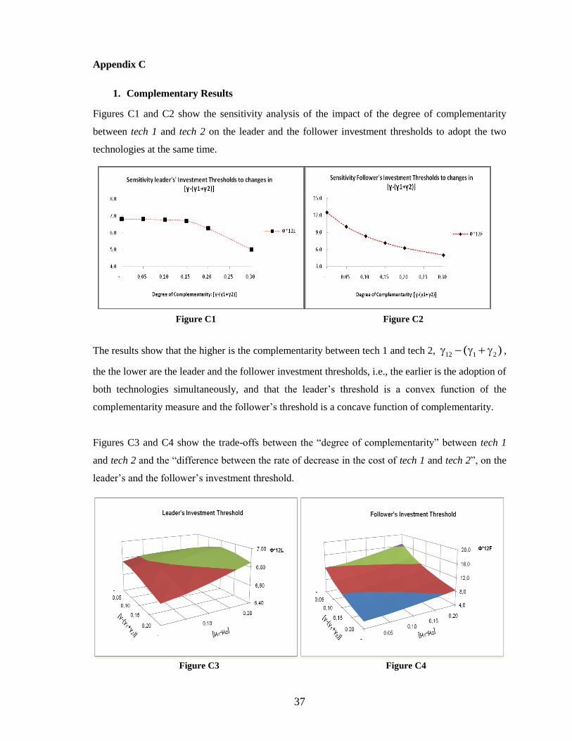
37
Appendix C
1. Complementary Results
Figures C1 and C2 show the sensitivity analysis of the impact of the degree of complementarity
between tech 1 and tech 2 on the leader and the follower investment thresholds to adopt the two
technologies at the same time.
Figure C1 Figure C2
The results show that the higher is the complementarity between tech 1 and tech 2, 12 1 2( ) ,
the the lower are the leader and the follower investment thresholds, i.e., the earlier is the adoption of
both technologies simultaneously, and that the leader’s threshold is a convex function of the
complementarity measure and the follower’s threshold is a concave function of complementarity.
Figures C3 and C4 show the trade-offs between the “degree of complementarity” between tech 1
and tech 2 and the “difference between the rate of decrease in the cost of tech 1 and tech 2”, on the
leader’s and the follower’s investment threshold.
Figure C3 Figure C4

38
Although the scales are somewhat different for the leader and the follower, the leader’s
simultaneous thresholds appear to eventually be insensitive to lower complementarity and greater
drift differences, while the follower’s thresholds reach a peak at nil complementarity and large drift
differences.
References
Anderson, E., Schmittlein, D., 1984. Integration of Sales Force: An Empirical Examination. Rand
Journal of Economics 15, 385-395.
Arora, A., 1996. Testing for Complementarities in Reduced-Form Regressions: A Note. Economic
Letters 50, 51-55.
Arora, A., Gambardella, A., 1990. Complementarity and External Linkages: the Strategies of the
Large Firms in Biotechnology. Journal of Industrial Economics 38, 361-379.
Azevedo, A., Paxson, D., 2008. New Technology Adoption Games: An Aplication to the Textile
Industry: Presented at the Real Options Conference 2008, Pontifícia Universidade Católica, Rio
de Janeiro.
Azevedo, A., Paxson, D., 2010. Developing Real Option Game Models: Presented at the Real
Options Conference 2010, Luiss Business School, University of Rome, Rome.
Braga, H., Wilmore, L., 1991. Technological Imports and Technological effort: An Analysis of their
Determinants in Brazilian Firms. Journal of Industrial Economics 39, 421-432.
Carree, M., Lokshin, B., Belderbos, R., 2010. A Note on Testing for Complementarity and
Substitutability in the Case of Multiple Practices. Journal of Productivity Analysis Published
online, 20 July 2010.
Cassiman, B., Veugelers, E., 2004. In Search of Complementarity in Innovation Strategy: Internal
R&D and External Knowledge Acquisition, Working Paper, University of Leuven.
Cho, Soo-Haeng and McCardle, K. (2009). The Adoption of Multiple Dependent Technologies.
Operations Research 57, 157-169.
Colombo, M., Mosconi, R., 1995. Complementarity and Cumulative Learning Effects in the Early
Diffusion of Multiple Technologies. Journal of Industrial Economics 43, 13-48.
Cooper, I., 2006. Asset Pricing Implications of Nonconvex Adjustment Costs and Irreversibility of
Investment. Journal of Finance 61, 139-170
Dixit, A., Pindyck, R., 1994. Investments under Uncertainty. Princeton NJ, Princeton University
Press.
Etro, F., 2007. Competition, Innovation, and Antitrust: A Theory of Market Leaders and its Policy
Implication, Berlin, Springer.

39
Fudenberg, D., Tirole, J., 1985. Preemption and Rent Equalization in the Adoption of New
Technology. Review of Economic Studies 52, 383-401.
Gibbons, R., 1992. A Primer in Game Theory, London, FT - Prentice Hall.
Grenadier, S., 1996. The Strategic Exercise of Options: Development Cascades and Overbuilding in
Real Estate Markets. Journal of Finance 51, 1653-1679.
Huisman, K., 2001. Technology Investment: A Game Theoretical Options Approach, Boston,
Kluwer.
Jovanovic, B., Stolyarov, D., 2000. Optimal Adoption of Complementary Technologies. American
Economic Review 90, 15-29.
Lambrecht, B., Perraudin, W., 2003. Real Options and Preemption under Incomplete Information.
Journal of Economic Dynamics and Control 27, 619-643.
Mason, R. and Weeds, H., 2010, Investment, Uncertainty and Preemption. Journal of Industrial
Organization 28, 278-287.
Milgrom, P., Roberts, J., 1990. Economics of Modern Manufacturing: Technology, Strategy, and
Organization. American Economic Review 80, 511-528.
Milgrom, P., Roberts, J., 1994. Complementarities and Systems: Understanding Japanese Economic
Organization. Working Paper, Stanford University.
Milgrom, P., Roberts, J., 1995. Complementarities and Fit Strategy, Structure, and Organizational
Change in Manufacturing. Journal of Accounting and Economics 19, 179-208.
Miravete, E., Pernías, J., 1998. Innovation Complementarity and Scale of Production. Working
Paper, Center for Applied Economics, New York University.
Miravete, E., Pernías, J., 2010. Testing for Complementarity when Strategies are Dichotomous.
Economic Letters 106, 28-31.
Mohnen, P., Roller, L., 2000. Complementarity in Innovation Policy. Working Paper, University of
Quebec.
Morettto, M., 2008. Competition and Irreversible Investments under Uncertainty. Information
Economics and Policy 20, 75-88.
Paxson, D., Pinto, H., 2005. Rivalry under Price and Quantity Uncertainty, Review of Financial
Economics 14, 209-224.
Pawlina, G., Kort, P., 2006. Real options in an Asymmetric Duopoly: Who Benefits from your
Competitive Advantage? Journal of Economics and Management Studies 15, 1-35.
Smets, F., 1993. Essays on Foreign Direct Investment. PhD thesis, Yale University.
Smith, M., 2005. Uncertainty and the Adoption of Complementary Technologies. Industrial and
Corporate Change 14, 1-12.

40
Smith, M., Weil, D., 2005. Ratcheting Up: Linked Technology Adoption in Supply Chains.
Industrial Relations 44, 490-508.
Susan, A., Stern, S., 1998. An Empirical Framework for Testing Theories about Complementarity
in Organizational Design. Working Paper, MIT Sloan School of Management.
Sydsaeter, K., P. Hammond., 2006, Mathematics for Economic Analysis, Englewood Cliffs NJ,
Prentice-Hall.
Weeds, H., 2002. Strategic Delay in a Real Options Model of R&D Competition. Review of
Economic Studies. 69, 729-747.