uncertainty quantification in data-driven simulation and
TRANSCRIPT

Uncertainty Quantification in Data-Driven Simulation and
Optimization: Statistical and Computational Efficiency
Huajie Qian
Submitted in partial fulfillment of the
requirements for the degree of
Doctor of Philosophy
under the Executive Committee
of the Graduate School of Arts and Sciences
COLUMBIA UNIVERSITY
2020

c©2020
Huajie Qian
All Rights Reserved

ABSTRACT
Uncertainty Quantification in Data-Driven Simulation and
Optimization: Statistical and Computational Efficiency
Huajie Qian
Models governing stochasticity in various systems are typically calibrated from data, therefore
are subject to statistical errors/uncertainties which can lead to inferior decision making. This thesis
develops statistically and computationally efficient data-driven methods for problems in stochastic
simulation and optimization to quantify and hedge impacts of these uncertainties.
The first half of the thesis focuses on efficient methods for tackling input uncertainty which refers
to the simulation output variability arising from the statistical noise in specifying the input models.
Due to the convolution of the simulation noise and the input noise, existing bootstrap approaches
consist of a two-layer sampling and typically require substantial simulation effort. Chapter 2
investigates a subsampling framework to reduce the required effort, by leveraging the form of the
variance and its estimation error in terms of the data size and the sampling requirement in each
layer. We show how the total required effort is reduced, and explicitly identify the procedural
specifications in our framework that guarantee relative consistency in the estimation, and the
corresponding optimal simulation budget allocations. In Chapter 3 we study an optimization-
based approach to construct confidence intervals for simulation outputs under input uncertainty.
This approach computes confidence bounds from simulation runs driven by probability weights
defined on the data, which are obtained from solving optimization problems under suitably posited
averaged divergence constraints. We illustrate how this approach offers benefits in computational
efficiency and finite-sample performance compared to the bootstrap and the delta method. While
resembling distributionally robust optimization, we explain the procedural design and develop tight
statistical guarantees via a generalization of the empirical likelihood method.

The second half develops uncertainty quantification techniques for certifying solution feasibility
and optimality in data-driven optimization. Regarding optimality, Chapter 4 proposes a statis-
tical method to estimate the optimality gap of a given solution for stochastic optimization as an
assessment of the solution quality. Our approach is based on bootstrap aggregating, or bagging,
resampled sample average approximation (SAA). We show how this approach leads to valid statis-
tical confidence bounds for non-smooth optimization. We also demonstrate its statistical efficiency
and stability that are especially desirable in limited-data situations. We present our theory that
views SAA as a kernel in an infinite-order symmetric statistic. Regarding feasibility, Chapter 5
considers data-driven optimization under uncertain constraints, where solution feasibility is often
ensured through a “safe” reformulation of the constraints, such that an obtained solution is guar-
anteed feasible for the oracle formulation with high confidence. Such approaches generally involve
an implicit estimation of the whole feasible set that can scale rapidly with the problem dimension,
in turn leading to over-conservative solutions. We investigate validation-based strategies to avoid
set estimation by exploiting the intrinsic low dimensionality of the set of all possible solutions
output from a given reformulation. We demonstrate how our obtained solutions satisfy statistical
feasibility guarantees with light dimension dependence, and how they are asymptotically optimal
and thus regarded as the least conservative with respect to the considered reformulation classes.

Table of Contents
List of Figures vi
List of Tables vii
Acknowledgements ix
1 Introduction 1
1.1 Stochastic Simulation under Input Uncertainty . . . . . . . . . . . . . . . . . . . . . 1
1.2 Uncertainty Quantification in Data-Driven Optimization . . . . . . . . . . . . . . . . 4
2 Subsampling to Enhance Efficiency in Input Uncertainty Quantification 7
2.1 Introduction . . . . . . . . . . . . . . . . . . . . . . . . . . . . . . . . . . . . . . . . . 7
2.2 Problem Motivation . . . . . . . . . . . . . . . . . . . . . . . . . . . . . . . . . . . . 11
2.2.1 Notation . . . . . . . . . . . . . . . . . . . . . . . . . . . . . . . . . . . . . . . 11
2.2.2 The Input Uncertainty Problem . . . . . . . . . . . . . . . . . . . . . . . . . . 11
2.2.3 Bootstrap Resampling . . . . . . . . . . . . . . . . . . . . . . . . . . . . . . . 14
2.2.4 A Complexity Barrier . . . . . . . . . . . . . . . . . . . . . . . . . . . . . . . 15
2.3 Procedures and Guarantees in the Subsampling Framework . . . . . . . . . . . . . . 18
2.3.1 Proportionate Subsampled Variance Bootstrap . . . . . . . . . . . . . . . . . 18
2.3.2 Statistical Guarantees . . . . . . . . . . . . . . . . . . . . . . . . . . . . . . . 21
2.4 Developments of Theoretical Results . . . . . . . . . . . . . . . . . . . . . . . . . . . 25
2.4.1 Regularity Assumptions . . . . . . . . . . . . . . . . . . . . . . . . . . . . . . 25
i

2.4.2 Simulation Complexity and Allocation . . . . . . . . . . . . . . . . . . . . . . 30
2.4.3 Optimal Subsample Ratio . . . . . . . . . . . . . . . . . . . . . . . . . . . . . 32
2.5 Numerical Experiments . . . . . . . . . . . . . . . . . . . . . . . . . . . . . . . . . . 36
2.5.1 Guidelines for Algorithmic Configuration . . . . . . . . . . . . . . . . . . . . 40
2.5.2 Comparisons with the Variance Bootstrap and the Percentile Bootstrap . . . 42
2.5.3 Constructing CI via Input Variance and Comparisons of the Splitting and
Nonsplitting Approaches . . . . . . . . . . . . . . . . . . . . . . . . . . . . . . 46
2.6 Conclusion . . . . . . . . . . . . . . . . . . . . . . . . . . . . . . . . . . . . . . . . . 49
3 Optimization-Based Quantification of Simulation Input Uncertainty via Empir-
ical Likelihood 50
3.1 Introduction . . . . . . . . . . . . . . . . . . . . . . . . . . . . . . . . . . . . . . . . . 50
3.2 Related Literature . . . . . . . . . . . . . . . . . . . . . . . . . . . . . . . . . . . . . 53
3.3 Optimization-Based Confidence Intervals . . . . . . . . . . . . . . . . . . . . . . . . . 54
3.3.1 Problem Setting . . . . . . . . . . . . . . . . . . . . . . . . . . . . . . . . . . 54
3.3.2 Main Procedure . . . . . . . . . . . . . . . . . . . . . . . . . . . . . . . . . . 56
3.3.3 Statistical Guarantees . . . . . . . . . . . . . . . . . . . . . . . . . . . . . . . 60
3.4 Theory on Statistical Guarantees . . . . . . . . . . . . . . . . . . . . . . . . . . . . . 64
3.4.1 An Initial Interpretation from DRO . . . . . . . . . . . . . . . . . . . . . . . 64
3.4.2 Linearization of Performance Measure . . . . . . . . . . . . . . . . . . . . . . 66
3.4.3 Empirical Likelihood Theory for Sums of Means . . . . . . . . . . . . . . . . 68
3.4.4 Duality and Optimization-Based Confidence Intervals . . . . . . . . . . . . . 71
3.4.5 Estimating Influence Function . . . . . . . . . . . . . . . . . . . . . . . . . . 74
3.4.6 Evaluation of CI Bounds . . . . . . . . . . . . . . . . . . . . . . . . . . . . . . 76
3.5 Numerical Experiments . . . . . . . . . . . . . . . . . . . . . . . . . . . . . . . . . . 79
3.5.1 Mean Waiting Time of an M/M/1 Queue . . . . . . . . . . . . . . . . . . . . 81
3.5.2 Stochastic Activity Networks . . . . . . . . . . . . . . . . . . . . . . . . . . . 85
3.5.3 Summary and Comparisons with the Bootstrap . . . . . . . . . . . . . . . . . 89
ii

3.6 Conclusion . . . . . . . . . . . . . . . . . . . . . . . . . . . . . . . . . . . . . . . . . 91
4 Bounding Optimality Gap in Stochastic Optimization via Bagging 93
4.1 Introduction . . . . . . . . . . . . . . . . . . . . . . . . . . . . . . . . . . . . . . . . . 93
4.2 Existing Challenges and Motivation . . . . . . . . . . . . . . . . . . . . . . . . . . . 97
4.2.1 Using Asymptotics of Sample Average Approximation . . . . . . . . . . . . . 98
4.2.2 Batching Procedures . . . . . . . . . . . . . . . . . . . . . . . . . . . . . . . . 100
4.2.3 Motivation and Overview of Our Approach . . . . . . . . . . . . . . . . . . . 101
4.3 Bagging Procedure to Estimate Optimal Values . . . . . . . . . . . . . . . . . . . . . 102
4.4 SAA as Symmetric Kernel . . . . . . . . . . . . . . . . . . . . . . . . . . . . . . . . . 104
4.5 Asymptotic Behaviors with Growing Resample Size . . . . . . . . . . . . . . . . . . . 108
4.6 Statistical Properties of Bagging Bounds and Comparisons with Batching . . . . . . 113
4.7 Error Estimates and Coverages . . . . . . . . . . . . . . . . . . . . . . . . . . . . . . 116
4.8 Numerical Experiments . . . . . . . . . . . . . . . . . . . . . . . . . . . . . . . . . . 118
4.8.1 Lower Bounds of Optimal Values . . . . . . . . . . . . . . . . . . . . . . . . . 120
4.8.2 Upper Bounds of Optimality Gaps . . . . . . . . . . . . . . . . . . . . . . . . 123
4.9 Conclusion . . . . . . . . . . . . . . . . . . . . . . . . . . . . . . . . . . . . . . . . . 126
5 Combating Conservativeness in Optimization with Uncertain Constraints 128
5.1 Introduction . . . . . . . . . . . . . . . . . . . . . . . . . . . . . . . . . . . . . . . . . 128
5.1.1 Existing Frameworks and Motivation of Our Approach . . . . . . . . . . . . . 129
5.2 Overview of Our Framework and Rationale . . . . . . . . . . . . . . . . . . . . . . . 135
5.3 Validation via Multivariate Gaussian Supremum . . . . . . . . . . . . . . . . . . . . 137
5.3.1 Performance Guarantees for General Stochastic Constraints . . . . . . . . . . 139
5.3.2 Performance Guarantees for Chance Constraints . . . . . . . . . . . . . . . . 142
5.4 Validation via Univariate Gaussian Margin . . . . . . . . . . . . . . . . . . . . . . . 144
5.4.1 Asymptotic Performance Guarantees . . . . . . . . . . . . . . . . . . . . . . . 145
5.5 Applying Our Framework in Data-Driven Reformulations . . . . . . . . . . . . . . . 152
5.6 Numerical Experiments . . . . . . . . . . . . . . . . . . . . . . . . . . . . . . . . . . 161
iii

5.6.1 RO and SCA . . . . . . . . . . . . . . . . . . . . . . . . . . . . . . . . . . . . 162
5.6.2 Moment-Based DRO . . . . . . . . . . . . . . . . . . . . . . . . . . . . . . . . 164
5.6.3 SO . . . . . . . . . . . . . . . . . . . . . . . . . . . . . . . . . . . . . . . . . . 165
5.7 Conclusion . . . . . . . . . . . . . . . . . . . . . . . . . . . . . . . . . . . . . . . . . 167
Bibliography 169
Appendices 181
A Technical Proofs for Chapter 2 181
A.1 Finite-Horizon Performance Measures . . . . . . . . . . . . . . . . . . . . . . . . . . 181
A.2 Proofs of Propositions 2.4.1 and 2.4.6 . . . . . . . . . . . . . . . . . . . . . . . . . . 194
A.3 Proofs for Results in Section 2.4.2 and Section 2.3.2 . . . . . . . . . . . . . . . . . . 196
A.4 Proofs for Results in Section 2.4.3 and Theorem 2.3.6 . . . . . . . . . . . . . . . . . 199
B Technical Proofs for Chapter 3 205
B.1 Notation and Outline . . . . . . . . . . . . . . . . . . . . . . . . . . . . . . . . . . . . 205
B.2 Proofs of Results in Section 3.4.2 . . . . . . . . . . . . . . . . . . . . . . . . . . . . . 207
B.3 Proof of Results in Section 3.4.3 . . . . . . . . . . . . . . . . . . . . . . . . . . . . . 217
B.4 Proofs of Results in Section 3.4.4 . . . . . . . . . . . . . . . . . . . . . . . . . . . . . 229
B.5 Proofs of Results in Section 3.4.5 . . . . . . . . . . . . . . . . . . . . . . . . . . . . . 236
B.6 Proofs of Results in Section 3.4.6 . . . . . . . . . . . . . . . . . . . . . . . . . . . . . 243
B.7 Proofs of Proposition 3.3.1 and Theorems 3.3.2, 3.3.3, 3.3.4 . . . . . . . . . . . . . . 248
C Technical Proofs for Chapter 4 256
C.1 Proof of Lemma 4.5.1 . . . . . . . . . . . . . . . . . . . . . . . . . . . . . . . . . . . 256
C.2 Proof of Theorems 4.5.2 and 4.5.3 . . . . . . . . . . . . . . . . . . . . . . . . . . . . 261
C.3 Proof of Theorems 4.5.4 and 4.5.5 . . . . . . . . . . . . . . . . . . . . . . . . . . . . 272
C.4 Proof of Proposition 4.6.1 . . . . . . . . . . . . . . . . . . . . . . . . . . . . . . . . . 280
C.5 Proof of Theorem 4.6.2 and the Claim in Example 4.6.1 . . . . . . . . . . . . . . . . 280
iv

C.6 Proof of Theorem 4.6.4 . . . . . . . . . . . . . . . . . . . . . . . . . . . . . . . . . . . 282
C.7 Proof of Theorems 4.7.1 and 4.7.2 . . . . . . . . . . . . . . . . . . . . . . . . . . . . 283
C.8 Proof of Theorem 4.7.3 and Corollary 4.7.4 . . . . . . . . . . . . . . . . . . . . . . . 289
D Technical Proofs for Chapter 5 293
D.1 Existing Central Limit Theorems in High Dimensions . . . . . . . . . . . . . . . . . 293
D.2 Proofs of Results in Section 5.3 . . . . . . . . . . . . . . . . . . . . . . . . . . . . . . 295
D.2.1 A CLT for Random Vectors with Potentially Small Variances . . . . . . . . . 295
D.2.2 CLTs for Sample Means Normalized by Standard Deviations . . . . . . . . . 297
D.2.3 Coverage Probability through Multiplier Bootstrap . . . . . . . . . . . . . . . 307
D.2.4 Proofs of Main Statistical Guarantees . . . . . . . . . . . . . . . . . . . . . . 310
D.3 Proofs of Results in Section 5.4 . . . . . . . . . . . . . . . . . . . . . . . . . . . . . . 315
D.4 Proofs of Results in Section 5.5 . . . . . . . . . . . . . . . . . . . . . . . . . . . . . . 332
D.5 Finite Sample Performance Guarantees for Univariate Gaussian Validator . . . . . . 344
D.5.1 Differentiable Constraints . . . . . . . . . . . . . . . . . . . . . . . . . . . . . 344
D.5.2 Linear Chance Constraints . . . . . . . . . . . . . . . . . . . . . . . . . . . . 355
D.6 Applying Univariate Gaussian Validator to Formulations with Multidimensional Con-
servativeness Parameters . . . . . . . . . . . . . . . . . . . . . . . . . . . . . . . . . . 364
v

List of Figures
1.1 Distribution of upper confidence bounds, relative to the threshold 2.5. . . . . . . . . 3
2.1 A computer network with four nodes and four channels. . . . . . . . . . . . . . . . . 37
2.2 Input variance estimation accuracy under different configurations of B,R such that
BR = 1000. . . . . . . . . . . . . . . . . . . . . . . . . . . . . . . . . . . . . . . . . . 40
2.3 Input variance estimation accuracy under different subsample sizes with B,R opti-
mally tuned. . . . . . . . . . . . . . . . . . . . . . . . . . . . . . . . . . . . . . . . . . 41
2.4 Monotonicity between coverage accuracy and input variance estimation accuracy. . . 46
2.5 Coverage comparison under the splitting and nonsplitting approaches. . . . . . . . . 48
2.6 Coverage probability versus CI width, under different budget splits in the form of
“Rv +Re”. . . . . . . . . . . . . . . . . . . . . . . . . . . . . . . . . . . . . . . . . . 49
3.1 Stochastic activity networks. . . . . . . . . . . . . . . . . . . . . . . . . . . . . . . . 86
vi

List of Tables
2.1 True arrival rates λi,j of messages to be transmitted from node i to node j. . . . . . 38
2.2 Results for the M/M/1 queue with arrival rate 0.5 and service rate 1. . . . . . . . . 43
2.3 Results for the M/M/1 queue with arrival rate 0.9 and service rate 1. . . . . . . . . 43
2.4 Results for the computer network. . . . . . . . . . . . . . . . . . . . . . . . . . . . . 43
3.1 M/M/1 queue. n1 = 30, n2 = 25. Total simulation budget 2000. Run times (sec-
ond/CI): three EL methods 1.1 × 10⁻², the bootstrap 1.2 × 10⁻², delta method
1.0× 10⁻². . . . . . . . . . . . . . . . . . . . . . . . . . . . . . . . . . . . . . . . . . 83
3.2 M/M/1 queue. n1 = 120, n2 = 100. Total simulation budget 8000. Run times
(second/CI): three EL methods 4.0× 10⁻², the bootstrap 3.4× 10⁻², delta method
5.3× 10⁻². . . . . . . . . . . . . . . . . . . . . . . . . . . . . . . . . . . . . . . . . . 84
3.3 M/M/1 queue. n1 = 30, n2 = 25. . . . . . . . . . . . . . . . . . . . . . . . . . . . . . 85
3.4 Stochastic activity network in Figure 3.1a. n1 = n2 = 200, n3 = n4 = n5 = 30. Total
simulation budget 8000. Run times (second/CI): three EL methods 3.3× 10⁻², the
bootstrap 1.7× 10⁻², delta method 3.2× 10⁻². . . . . . . . . . . . . . . . . . . . . . 86
3.5 Stochastic activity network in Figure 3.1b. ni = 30 for 1 ≤ i ≤ 7 and 25 for
8 ≤ i ≤ 14. Total simulation budget 4000. Run times (second/CI): three EL
methods 2.7× 10⁻², the bootstrap 2.7× 10⁻², delta method 1.7× 10⁻². . . . . . . . 88
3.6 Tail probability of stochastic activity network in Figure 3.1b. ni = 120 for 1 ≤ i ≤ 7
and 100 for 8 ≤ i ≤ 14. Total simulation budget 16000. Run times (second/CI):
three EL methods 0.11, the bootstrap 0.03, delta method 0.10. . . . . . . . . . . . . 89
vii

3.7 Tail probability of stochastic activity network in Figure 3.1b. ni = 480 for 1 ≤ i ≤ 7
and 400 for 8 ≤ i ≤ 14. Total simulation budget 60000. Run times (second/CI):
three EL methods 1.4, the bootstrap 0.08, delta method 1.3. . . . . . . . . . . . . . . 90
4.1 Problem (4.21), n = 50. Lower bounds of optimal values. . . . . . . . . . . . . . . . 121
4.2 Problem (4.21), n = 300. Lower bounds of optimal values. . . . . . . . . . . . . . . . 121
4.3 Problem (4.24), n = 100. Lower bounds of optimal values. . . . . . . . . . . . . . . . 122
4.4 Problem (4.22), n = 40, n1 = 20, n2 = 20. Upper bounds of optimality gaps by BC. . 123
4.5 Problem (4.22), n = 40, n1 = 20, n2 = 20. Upper bounds of optimality gaps by CRN. 123
4.6 Problem (4.23), n = 100, n1 = 64, n2 = 36. Upper bounds of optimality gaps by BC. 124
4.7 Problem (4.23), n = 100, n1 = 64, n2 = 36. Upper bounds of optimality gaps by CRN.124
4.8 Problem (4.24), n = 100, n1 = 64, n2 = 36. Upper bounds of optimality gaps by BC. 125
4.9 Problem (4.24), n = 100, n1 = 64, n2 = 36. Upper bounds of optimality gaps by CRN.125
5.1 RO with ellipsoidal uncertainty set. d = 10, n = 200. Data are split to n1 =
100, n2 = 100. . . . . . . . . . . . . . . . . . . . . . . . . . . . . . . . . . . . . . . . . 163
5.2 RO with ellipsoidal uncertainty set. d = 10, n = 500. Data are split to n1 =
250, n2 = 250. . . . . . . . . . . . . . . . . . . . . . . . . . . . . . . . . . . . . . . . . 163
5.3 RO with ellipsoidal uncertainty set. d = 50, n = 500. Data are split to n1 =
250, n2 = 250. . . . . . . . . . . . . . . . . . . . . . . . . . . . . . . . . . . . . . . . . 163
5.4 Moment-based DRO. d = 10, n = 200. Data are split to n1 = 100, n2 = 100. . . . . . 164
5.5 Moment-based DRO. d = 10, n = 500. Data are split to n1 = 250, n2 = 250. . . . . . 165
5.6 SO. d = 10, n = 200. Data are split to n1 = 150, n2 = 50. . . . . . . . . . . . . . . . . 165
5.7 SO. d = 10, n = 500. Data are split to n1 = 250, n2 = 250. . . . . . . . . . . . . . . . 166
5.8 FAST. d = 10, n = 200. Data are split to n1 = 100, n2 = 100. . . . . . . . . . . . . . 167
5.9 FAST. d = 50, n = 500. Data are split to n1 = 250, n2 = 250. . . . . . . . . . . . . . 167
viii

Acknowledgments
This thesis concludes my Ph.D. research over the past five years. I am indebted to many outstanding
scholars and individuals who have guided me through the rewarding journey.
First and foremost, I would like to express my deepest gratitude to my advisor, Professor Henry
Lam, for his enlightening, persistent, and comprehensive guidance throughout these years. He
has been constantly offering insightful advice with his enduring patience and broad knowledge in
simulation, optimization, statistics and beyond. As a statistician as well as an operations researcher,
his diverse perspectives on research questions have greatly helped me transition from a mathematical
background to operations research. He has also been extremely approachable and considerate, which
has made my Ph.D. study such a smooth and enjoyable experience. I have learnt from him a lot
on how to do research and be a scholar. All these have set him a role model for me in pursuit of
academic excellence.
I would like to thank Professor Jing Dong, Garud Iyengar, David Yao, and Xunyu Zhou for
serving on my thesis committee. Their constructive feedback and comments have led to great
improvement of this thesis in terms of both presentation and material. I have learnt much from
the insightful discussions with them.
I also want to extend my appreciation to many exceptional professors with whom I have taken
courses that lay the foundation for the research works in this thesis. I would like to thank Professor
Jinho Baik and David Yao for probability and stochastics, Professor Long Nguyen and Ambuj
Tewari for statistical and machine learning, Professor John Duchi and Ruiwei Jiang for theories
and algorithms for stochastic and robust optimizaton, and Professor Roman Vershynin for high
dimensional probability theory. I also thank Professor Kristen Moore and Virginia Young for their
guidance on stochastic control problems in mathematical finance, and Professor Donald Lee and
ix

David Yao for introducing impactful applications of statistical learning.
My sincere thanks also go to many friends and fellow students at Columbia University and
University of Michigan, and those I’ve luckily met at conferences. I thank all of you for the help
I’ve received in both research and daily life, and for the many casual chats and academic discussions
that have contributed to this thesis in one way or another.
Lastly and most importantly, I thank my parents, Huifa Qian and Jinmei Fan, and my wife,
Xiaochen Wang, for their unconditional love and support. Besides emotional support, I have learnt
much about statistics from my wife, who recently earned her Ph.D. in biostatistics.
x

Dedicated to my father, Huifa Qian, and my wife, Xiaochen Wang.
In loving memory of my mother, Jinmei Fan.
xi

CHAPTER 1. INTRODUCTION 1
Chapter 1
Introduction
In the data-rich era, decision making under uncertainty often relies on inference of unknown stochas-
ticity from real-world data. A common concern, however, is that the model and statistical errors
from the data may not be properly controlled when integrating into the downstream simulation and
optimization tasks, thus leading to inferior decisions. Therefore a quantitative understanding of the
statistical uncertainties is crucial in guarding against catastrophic decision making. Broadly speak-
ing, this has stimulated interests across multiple research communities, and various approaches
have been proposed to handle statistical uncertainties for different kinds of problems, such as un-
certainty sets in (distributionally) robust opotimization, penalties in regularized risk minimization,
and upper confidence bound (UCB) algorithms in reinforcement learning. This thesis instead in-
vestigates uncertainty quantification methods for two commonly used tools in operations research,
i.e., stochastic simulation (in Chapters 2 and 3) and optimization under uncertainty (in Chapters
4 and 5), and focuses on statistical and/or computational efficiencies of these methods.
1.1 Stochastic Simulation under Input Uncertainty
The first part (Chapters 2 and 3) of the thesis is on efficient methods for tackling input uncertainty
in stochastic simulation. Stochastic simulation has been used routinely to assess and optimize
performances of stochastic operational systems. In conventional simulation output analysis, the

CHAPTER 1. INTRODUCTION 2
underlying input models are assumed completely known or given by expert opinions, and simulation
outputs generated from these input models are used to make statistical inference on the performance
metric of interest. In a data-driven setting, however, input models are estimated from data to drive
simulation, and input uncertainty arises due to the propagation of the input estimation errors
to the output. Therefore, statistically valid inference and performance prediction require careful
incorporation of model errors on top of the stochastic computation noises in the Monte Carlo
simulation.
To further illustrate the necessity of tackling input uncertainty, consider an M/M/1 queue with
arrival rate 0.8 and service rate 1.0, and the performance measure of interest is the mean waiting
time of the first 20 arrivals (true value ≈ 2.57). Suppose that the true arrival and service rates
are unknown and can only be estimated from data of inter-arrival times and service times, each
of size 50, therefore input uncertainty is present. Suppose that a criterion in designing the queu-
ing system is that the mean waiting time must be no longer than 2.5 units of time (the current
design is infeasible). We compare two approaches to assessing feasibility of the current design,
both involving the construction of upper confidence bounds for the target quantity. In the first
approach, an arrival rate and a service rate are estimated from the data, and then treated as the
truth to drive the simulation to obtain a 95%-level performance bound based on 500 replications.
The experiment is then repeated on 1000 independent input data sets, and the distribution of the
obtained performance bounds are shown in Figure 1.1a. The second approach, however, acknowl-
edges the statistical errors in the estimated input models, and incorporate them in constructing
the performance bounds. The results are in Figure 1.1b. We observe that when input uncertainty
is ignored the obtained bounds often (44%) fall below the threshold 2.5, rendering a substantial
chance of incorrect feasibility assessment, whereas after incorporating input uncertainty misassess-
ment happens much less frequently (10%). Quantification of input uncertainty therefore is essential
for correctly hedging the total risk in the output.
There are several challenges in quantifying input uncertainty. The first is the computational
demand in disentangling the statistical noise in calibrating the input model from the Monte Carlo
noise. Previous approaches to this problem such as the bootstrap (Barton and Schruben (1993,

CHAPTER 1. INTRODUCTION 3
0 2 4 6 8 10 12 14 16 18
time
0
20
40
60
80
100
120Histogram of confidence bounds that ignore input uncertainty
waiting time = 2.5
(a) Input uncertainty ignored.
0 2 4 6 8 10 12 14 16 18
time
0
20
40
60
80
100
120Histogram of confidence bounds that incorporate input uncertainty
waiting time = 2.5
(b) Input uncertainty taken into account.
Figure 1.1: Distribution of upper confidence bounds, relative to the threshold 2.5.
2001), Cheng and Holland (1997)) require a substantial computation effort because of the need to
conduct multi-layer nested simulation and consequently a multiplicatively growing size of simulation
replications. Secondly, approaches based-on the delta method (e.g., Chapter 3 in Asmussen and
Glynn (2007) and Cheng and Holland (1997, 1998)) construct interval estimates from a linearization
of the performance metric and an estimation of the standard error term, which tend to undercover
the true performance metric under small input data. Chapters 2 and 3, respectively, are devoted
to addressing these challenges.
Chapter 2 develops a subsampling technique that significantly reduces the order of computation
in each layer of the nested simulation, by leveraging and properly rescaling the standard error arising
from input uncertainty according to the subsample size parameters. The proposed method provably
allows the simulation cost to grow independently of the data size, in contrast to the standard
bootstrap where the required simulation burden has to grow linearly, thus making our method
more attractive when each simulation run is computationally expensive or simulation resources are
limited. We also derive the optimal algorithmic configurations, regarding choices of the subsample
size and the simulation sizes to allocate to each layer, that achieve the minimum error in estimating
the input uncertainty under a fixed simulation budget, by balancing a trade-off between a Monte
Carlo (computational) error and a statistical error.
In Chapter 3 we propose an optimization-based approach that computes interval estimates as
the optimal values of suitably posited optimization problems which do not rely on linearization.

CHAPTER 1. INTRODUCTION 4
Our formulation is based on an “empirical” version of distributionally robust optimization (DRO).
The latter is a decision-making framework for stochastic problems where the underlying distribution
is not fully known, which advocates the search of the best solution over the worst-case scenario.
Our formulation constructs interval estimates by optimizing the performance metric over a set of
distributions that are supported on the input data, satisfying a suitably weighted Kullback-Leibler
divergence constraint. We demonstrate how our approach can conform naturally to the numerical
boundary of the performance metric and leads to better finite-sample coverage than linearization-
based interval estimates. Moreover, we develop tight coverage guarantees via a generalization of
the empirical likelihood theory, in contrast to potentially loose confidence guarantees in previous
data-driven DRO formulations.
1.2 Uncertainty Quantification in Data-Driven Optimization
In the second part (Chapters 4 and 5) we switch focus to uncertainty quantification for data-
driven optimization. Stochastic optimization has been extensively used for decision making under
uncertainty in both operations research and machine learning, where the decision maker optimizes a
certain expected performance measure, potentially subject to uncertain constraints. In the context
where the governing distributions are estimated from data, Chapters 4 and 5 investigate statistically
efficient methodologies to assess and improve solution performances in terms of optimality and
feasibility.
Chapter 4 presents a novel method based on bagging or bootstrap aggregating, an ensemble
method in machine learning, to compute bounds for the optimality gap of a given solution. The
motivation is that data-driven solutions to stochastic optimization can be suboptimal due to con-
tamination from statistical and model errors, and a quantitative assessment of solution quality can
help with screening out inferior solutions. The goal here is to assess solution performance by using
data; this is in contrast to the common analyses of stochastic optimization algorithms that reveal
the convergence rate, which are based on the worst-case and could be over-conservative for a given
particular problem instance. Existing methods based on data batching (Mak et al. (1999)) tend
CHAPTER 1. INTRODUCTION 5
to generate unnecessarily loose bounds due to the inefficient use of the data, while those based on
sample average approximation (SAA) asymptotics (Shapiro et al. (2014), Bayraksan and Morton
(2006)) require Lipschitz smoothness from the optimization and can perform poorly in practice
due to the instability in estimating the standard error. The proposed bagging method reduces the
estimation variance of optimality gap bounds and stabilizes estimation of the standard error by
averaging a large number of resampled estimates, and at the same time extends the SAA asymp-
totic theories to non-smooth problems by smoothing the SAA optimal values. Mathematically, we
established the asymptotic performance of our bagging approach by utilizing the so-called infinite-
order symmetric statistics, in which the SAA optimal value can be viewed as the kernel of the
corresponding statistics.
Chapter 5 focuses on improving data-driven solutions for optimization under uncertain con-
straints, such as probabilistic or expectation constraints. When these constraints are only observ-
able via data, feasibility can only be guaranteed at best with high confidence, and a data-driven
procedure needs to strike a balance between optimality and feasibility. Common data-driven for-
mulations, such as DRO, SAA, and robust optimization, ensure feasibility guarantees via a feasible
set estimation, or in other words, an implicit simultaneous estimation problem of the noisy con-
straint over the whole decision space. This could subsequently lead to over-conservative solutions
especially for high dimensional problems. To address this issue, we develop a general constraint-
validation framework that allows one to examine feasibility only on a low dimensional solution
path that is intrinsic to these common data-driven optimization formulations. We establish both
asymptotic and finite-sample performance guarantees of our framework, and dissect our results
to various formulations, by using recently developed high-dimensional Berry-Esseen theorem and
empirical process theory.
In the remainder of the thesis, Chapters 2-5 present in detail the four projects mentioned above,
and Appendices A-D contain technical proofs for each of the chapters respectively. As an effort
to improve the manageability of the notation system, mathematical symbols will be made self-
contained within each chapter, in other words, a symbol that refers to a certain object in one
chapter may be used to represent a different object in another chapter. The thesis is based on Lam

CHAPTER 1. INTRODUCTION 6
and Qian (2018c, 2017, 2018b, 2019a), for which preliminary versions have appeared in Lam and
Qian (2018d, 2016, 2018a, 2019b).

CHAPTER 2. SUBSAMPLING TO ENHANCE EFFICIENCY 7
Chapter 2
Subsampling to Enhance Efficiency in
Input Uncertainty Quantification
2.1 Introduction
Stochastic simulation is one of the most widely used analytic tools in operations research. It provides
a flexible means to approximate complex models and to inform decisions. See, for instance, Law
et al. (2000) and Banks et al. (2005) for applications in manufacturing, revenue management,
service and operations systems etc. In practice, the simulation platform relies on input models
that are typically observed or calibrated from data. These statistical noises can propagate to the
output analysis, leading to significant errors and suboptimal decision-making. In the literature,
this problem is commonly known as input uncertainty or extrinsic uncertainty.
In conventional simulation output analysis where the input model is completely pre-specified,
the statistical errors come solely from the Monte Carlo noises, and it suffices to account only
for such noises in analyzing the output variability. When input uncertainty is present, such an
analysis will undermine the actual variability. One common approach to quantify the additional
uncertainty is to estimate the variance in the output that is contributed from the input noises
(e.g., Song et al. (2014)); for convenience, we call this the input variance. This quantity acts as an
uncertainty measure which, when added together with the Monte Carlo variance, gives rise to the

CHAPTER 2. SUBSAMPLING TO ENHANCE EFFICIENCY 8
overall variance in the outputs. A refined decomposition of input variance across multiple input
sources can be used to identify models that are overly ambiguous and flag the need of more data
collection (e.g., Song et al. (2014)). Input variance also provides a building block to construct
valid output confidence intervals (CIs) that account for combined input and simulation errors (e.g.,
Cheng and Holland (2004)). Motivated by its central role in quantifying input uncertainty, this
chapter aims to study the efficient estimation of input variance.
In the literature, bootstrap resampling is a common approach for the above purpose. This
applies most prominently in the nonparametric regime, namely when no assumptions are placed
on the input parametric family. It could also be used in the parametric case (where more alter-
natives are available). For example, Cheng and Holland (1997) proposes the variance bootstrap,
and Song and Nelson (2015) studies the consistency of this strategy on a random-effect model that
describes the uncertainty propagation. A bottleneck with using bootstrap resampling in estimat-
ing input variances, however, is the need to “outwash” the simulation noise, which often places
substantial burden on the required simulation effort. More precisely, to handle both the input and
the simulation noises, the bootstrap procedure typically comprises a two-layer sampling that first
resamples the input data (i.e., outer sampling), followed by running simulation replications using
each resample (i.e., inner replications). Due to the reciprocal relation between the magnitude of
the input variance and the input data, the input variance becomes increasingly small as the input
data size increases. This deems the control of the relative estimation error increasingly expensive,
and requires either a large outer bootstrap size or inner replication size to extinguish the effect of
simulation noises.
The main goal of this chapter is to investigate subsampling as a simulation saver for input
variance estimation. This means that, instead of creating distributions by resampling a data set
of the full size, we only resample (with or without replacement) a set of smaller size. We show
that a judicious use of subsampling can reduce the total simulation effort from an order bigger
than the data size in the conventional two-layer bootstrap to an order independent of the data
size, while retaining the estimation accuracy. This approach leverages the interplay between the
form of the input variance and its estimation error, in terms of the data size and the sampling

CHAPTER 2. SUBSAMPLING TO ENHANCE EFFICIENCY 9
effort in each layer of the bootstrap. On a high level, the subsample is used to estimate an input
variance as if less data are available, followed by a correction of this discrepancy in the data size by
properly rescaling the input variance. We call this approach proportionate subsampled variance
bootstrap. We explicitly identify the procedural specifications in our approach that guarantee
estimation consistency, including the minimally required simulation effort in each layer. We also
study the theoretical behavior of our estimation error, in relation to the simulation effort allocation
in these layers as well as the input data and subsample sizes, which in turn reveals the optimal
configurations and provides implementation guidance.
In the statistics literature, subsampling has been used as a remedy for situations where the
full-size bootstrap does not apply, due to a lack (or undeterminability) of uniform convergence
required for its statistical consistency, which relates to the functional smoothness or regularity of
the estimators (e.g., Politis and Romano (1994)). Subsampling has been used in time series and
dependent data (e.g., Politis et al. (1999), Hall et al. (1995), Datta and McCormick (1995)), ex-
tremal estimation (e.g., Bickel and Sakov (2008)), shape-constrained estimation (e.g., Sen et al.
(2010)) and other econometric contexts (e.g., Abadie and Imbens (2008), Andrews and Guggen-
berger (2009, 2010)). In contrary to these works, our subsampling approach is introduced to reduce
the simulation effort faced by the two-layer sampling necessitated from the presence of both the
input and simulation noises. In other words, we are not concerned about the issue of uniform
convergence, but instead, we aim to distort the relation between the required simulation effort and
data size in a way that allows more efficient deconvolution of the effects of the two noises. We
also note that, as we will use resampling with replacement (instead of without replacement), our
approach is closer to the so-called m out of n bootstrap (Bickel et al. (1997), Bickel and Sakov
(2008)). For coherence, throughout the chapter we use the term subsampling broadly to indicate a
bootstrap with a smaller resample size than the original data size.
We close this introduction with a brief review of other related work in input uncertainty. In the
nonparametric regime (the focus of this chapter), besides Cheng and Holland (1997) and Song and
Nelson (2015) that study bootstrap-based estimation of the input variance, Barton and Schruben
(1993) and Barton and Schruben (2001) investigate the percentile bootstrap to construct CIs (i.e.,

CHAPTER 2. SUBSAMPLING TO ENHANCE EFFICIENCY 10
the CI limits are determined from the quantiles of the bootstrap distributions). Like variance boot-
strap, percentile bootstrap also encounters two-layer sampling that requires substantial simulation
efforts. Yi and Xie (2017) investigates adaptive budget allocation policies based on ranking and
selection to reduce simulation cost in the percentile bootstrap, and empirically shows the computa-
tional advantage of their approach. On the other hand, contrary to this work, they do not investigate
the required simulation efforts in relation to the input data size. Lam and Qian (2016, 2017) study
the use of empirical likelihood as an optimization-based alternative to the percentile bootstrap,
which requires simulation efforts to estimate the gradient information that remain substantial. Be-
yond the frequentist regime considered in this chapter, Xie et al. (2018) studies nonparametric
Bayesian methods based on Dirichlet process mixtures to estimate the variance contributed from
input uncertainty and construct CIs. Glasserman and Xu (2014), Hu et al. (2012), Lam (2016b)
and Ghosh and Lam (2019) study input uncertainty from a robust optimization viewpoint, where
they compute worst-case bounds subject to constraints or so-called uncertainty sets that represent
partial beliefs on unknown distributions. In the parametric regime, Barton et al. (2013) and Xie
et al. (2016) investigate the basic bootstrap with a metamodel built in advance, a technique known
as the metamodel-assisted bootstrap. Cheng and Holland (1997) studies the delta method, and
Cheng and Holland (1998, 2004) reduce its computation burden via the so-called two-point method.
Lin et al. (2015) and Song and Nelson (2019) study regression approaches to estimate sensitivity
coefficients which are used to apply the delta method, generalizing the gradient estimation method
in Wieland and Schmeiser (2006). Zhu et al. (2020) studies risk criteria and computation to quan-
tify parametric uncertainty. Finally, Chick (2001), Zouaoui and Wilson (2003), Zouaoui and Wilson
(2004) and Xie et al. (2014) study variance estimation and interval construction from a Bayesian
perspective. We comment that although the exposition in this chapter focuses on the nonparamet-
ric setting, the same idea of subsampling can be adapted naturally to the parametric setting, with
similar advantages in computational efficiency. For general surveys on input uncertainty, readers
are referred to Barton et al. (2002), Henderson (2003), Chick (2006), Barton (2012), Song et al.
(2014), Lam (2016a), and Nelson (2013) Chapter 7.
The remainder of this chapter is as follows. Section 2.2 introduces the input uncertainty problem

CHAPTER 2. SUBSAMPLING TO ENHANCE EFFICIENCY 11
and explains the simulation complexity bottleneck in the existing bootstrap schemes. Section 2.3
presents our subsampling idea, procedures and the main statistical results. Section 2.4 discusses
the key steps in our theoretical developments. Section 2.5 reports our numerical experiments. All
proofs are relegated to Appendix A.
2.2 Problem Motivation
This section describes the problem and our motivation. Section 2.2.2 first describes the input
uncertainty problem, Section 2.2.3 presents the existing bootstrap approach, and Section 2.2.4
discusses its computational barrier, thus motivating our subsampling investigation. We aim to
provide intuitive explanations in this section, and defer mathematical details to later sections.
2.2.1 Notation
We use the following notations. For any sequences an and bn, both depending on n, we say that
an = O(bn) if |an/bn| ≤ C for some constant C > 0 for all sufficiently large n, and an = o(bn) if
an/bn → 0 as n → ∞. Alternately, we say an = Ω(bn) if |an/bn| ≥ C for some constant C > 0
for all sufficiently large n, and an = ω(bn) if |an/bn| → ∞ as n → ∞. We say that an = Θ(bn)
if C ≤ |an/bn| ≤ C as n → ∞ for some constants C,C > 0. We use An = Op(bn) to represent
a sequence of random variables An that has stochastic order at least bn, i.e., for any ε > 0, there
exists M,N > 0 such that P (|An/bn| ≤ M) > 1 − ε for n > N . We use An = op(bn) to represent
a sequence of random variables An that has stochastic order less than bn, i.e., An/bnp→ 0. We use
An = Θp(bn) to represent a sequence An that has stochastic order exactly at bn, i.e., An satisfies
An = Op(bn) but not An = op(bn).
2.2.2 The Input Uncertainty Problem
Suppose there are m independent input processes driven by input distributions F1, F2, . . . , Fm.
We consider a generic performance measure ψ(F1, . . . , Fm) that is simulable, i.e., given the input
distributions, independent unbiased replications of ψ can be generated in a computer. As a primary

CHAPTER 2. SUBSAMPLING TO ENHANCE EFFICIENCY 12
example, think of F1 and F2 as the interarrival and service time distributions in a queue, and ψ is
some output measure such as the mean queue length averaged over a time horizon.
The input uncertainty problem arises in situations where the input distributions F1, . . . , Fm are
unknown but real-world data are available. One then has to use their estimates F1, . . . , Fm to drive
the simulation. Denote a point estimate of ψ(F1, . . . , Fm) as ψ(F1, . . . , Fm), where typically we
take
ψ(F1, . . . , Fm) =1
q
q∑r=1
ψr(F1, . . . , Fm)
with ψr(F1, . . . , Fm) being a conditionally unbiased simulation replication driven by F1, . . . , Fm.
This point estimate is affected by both the input statistical noises and the simulation noises. By
conditioning on the estimated input distributions (or viewing the point estimate as a random
effect model with uncorrelated input and simulation noises), the variance of ψ(F1, . . . , Fm) can be
expressed as
Var[ψ(F1, . . . , Fm)] = σ2I + σ2
S
where
σ2I = Var[ψ(F1, . . . , Fm)] (2.1)
is the input variance, and
σ2S =
E[Var[ψr(F1, . . . , Fm)|F1, . . . , Fm]]
q
is the variance contributed from the simulation noises. Assuming that the estimates Fi’s are
consistent in estimating Fi’s, then, as ni grows, σ2S is approximately Var[ψr(F1, . . . , Fm)]/q and
can be estimated by taking the sample variance of all simulation replications (see, e.g., Cheng and
Holland (1997)). On the other hand, σ2I signifies the output variance contributed solely from the
input data noises, assuming a fully accurate evaluation of the performance measure ψ. Estimating
σ2I is the key and the challenge in quantifying input uncertainty, which is the focus of this chapter.
Before going into details, we discuss two conceptual properties on σ2I that would be relevant in
motivating and pinpointing our study. First, suppose further that for each input model i, we have

CHAPTER 2. SUBSAMPLING TO ENHANCE EFFICIENCY 13
ni i.i.d. data Xi,1, . . . , Xi,ni generated from the distribution Fi. When ni’s are large, typically
the overall input variance σ2I is decomposable into
σ2I ≈
m∑i=1
σ2i
ni(2.2)
where σ2i /ni is the variance contributed from the data noise for model i, with σ2
i being a constant. In
the parametric case where Fi comes from a parametric family containing the estimated parameters,
this decomposition is well known from the delta method (Asmussen and Glynn (2007), Chapter 3).
Here, σ2i /ni is typically ∇iψ′Σi∇iψ, where ∇iψ is the collection of sensitivity coefficients, i.e., the
gradient, with respect to the parameters in model i, and Σi is the asymptotic estimation variance
of the point estimates of these parameters (scaled reciprocally with ni). In the nonparametric
case where the empirical distribution Fi(x) :=∑ni
j=1 δXi,j (x)/ni is used (where δXi,j denotes the
delta measure at Xi,j), (2.2) still holds under mild conditions (e.g., Propositions 2.4.1 and 2.4.6 in
the sequel). In this setting the quantity σ2i is equal to VarFi [gi(Xi)], where gi(·) is the influence
function (Hampel (1974)) of ψ with respect to the distribution Fi, whose domain is the value space
of the input variate Xi, and VarFi [·] denotes the variance under Fi. The influence function can
be viewed as a functional derivative taken with respect to the probability distributions Fi’s (see
Serfling (2009), Chapter 6), and dictates the first-order asymptotic behavior of the plug-in estimate
of ψ. Although the mathematical form of σ2i ’s is known, it relies on gradient information that needs
to be estimated via simulation itself. Moreover, in the nonparametric case, the gradient dimension
in a sense grows with the data size. Thus directly using the delta method in this case could be
challenging. In our subsequent developments, we focus on the nonparametric case, both because
this is more challenging, and also that this can be viewed as a generalization of the parametric case
by viewing the “parameter” simply as a function of Fi’s.
Second, under further regularity conditions, a Gaussian approximation holds for ψ(F1, . . . , Fm)
so that
ψ(F1, . . . , Fm)± z1−α/2
√σ2I + σ2
S (2.3)
is an asymptotically tight (1− α)-level CI for ψ(F1, . . . , Fm), where z1−α/2 is the standard normal

CHAPTER 2. SUBSAMPLING TO ENHANCE EFFICIENCY 14
1−α/2 quantile. This CI, which provides a bound-based alternative to quantify input uncertainty,
again requires a statistically valid estimate of σ2I or
∑mi=1 σ
2i /ni (and σ2
S). In this chapter we
primarily focus on the estimation of σ2I and how our proposed approach substantially improves
upon previous methods in this regard. Naturally, the improved estimate of σ2I also translates into
a better CI when using (2.3). We caution, however, that an optimal procedural configuration to
estimate σ2I does not necessarily correspond to an optimal configuration in constructing the CI, as
the performance of the latter is measured by different criteria such as coverage or half-width (such
a difference in optimally estimating variance versus CI has also been observed in other contexts
such as time series (Sun et al. (2008))). Nonetheless, we will show that a direct plug-in of our new
estimator of σ2I into (2.3) is already enough to significantly outperform conventional bootstrap-
based CIs suggested in the literature, both theoretically and also supported by consistent empirical
evidence.
Next we will discuss bootstrap resampling, the commonest estimation technique that forms the
basis of our comparison.
2.2.3 Bootstrap Resampling
Let F ∗i represent the empirical distribution constructed using a bootstrap resample from the original
data Xi,1, . . . , Xi,ni for input Fi, i.e., ni points drawn by uniformly sampling with replacement
from Xi,1, . . . , Xi,ni. The bootstrap variance estimator is Var∗[ψ(F ∗1 , . . . , F∗m)], where Var∗[·]
denotes the variance over the bootstrap resamples from the data, conditional on F1, . . . , Fm.
The principle of bootstrap entails that Var∗[ψ(F ∗1 , . . . , F∗m)] ≈ Var[ψ(F1, . . . , Fm)] = σ2
I . Here
Var∗[ψ(F ∗1 , . . . , F∗m)] is obtained from a (hypothetical) infinite number of bootstrap resamples and
simulation runs per resample. In practice, however, one would need to use a finite bootstrap size
and a finite simulation size. This comprises B conditionally independent bootstrap resamples of
F ∗1 , . . . , F ∗m, and R simulation replications driven by each realization of the resampled input
distributions. This generally incurs two layers of Monte Carlo errors.
Denote ψr(Fb1 , . . . , F
bm) as the r-th simulation run driven by the b-th bootstrap resample. Denote
ψb as the average of the R simulation runs driven by the b-th resample, and ¯ψ as the grand sample

CHAPTER 2. SUBSAMPLING TO ENHANCE EFFICIENCY 15
average from all the BR runs. An unbiased estimator for Var∗[ψ(F ∗1 , . . . , F∗m)] is given by
1
B − 1
B∑b=1
(ψb − ¯ψ)2 − V
R(2.4)
where
V =1
B(R− 1)
B∑b=1
R∑r=1
(ψr(Fb1 , . . . , F
bm)− ψb)2.
To explain, the first term in (2.4) is an unbiased estimate of the variance of ψb, which can be
expressed as Var∗[ψ(F ∗1 , . . . , F∗m)] + (1/R)E∗[Var[ψr(F
∗1 , . . . , F
∗m)|F ∗1 , . . . , F ∗m]] (where E∗[·] denotes
the expectation on F ∗i ’s conditional on Fi’s), since ψb incurs both the bootstrap noise and the
simulation noise. In other words, the variance of ψb is upward biased for Var∗[ψ(F ∗1 , . . . , F∗m)]. The
second term in (2.4), namely V/R, removes this bias. This bias adjustment can be derived by view-
ing Var∗[ψ(F ∗1 , . . . , F∗m)] as the variance of a conditional expectation. Alternately, ψr(F
∗1 , . . . , F
∗m)
can be viewed as a random effect model where each “group” corresponds to each realization of
F ∗1 , . . . , F∗m, and (2.4) estimates the “between-group” variance in an analysis-of-variance (ANOVA).
Formula (2.4) has appeared in the input uncertainty literature, e.g., Cheng and Holland (1997),
Song and Nelson (2015), Lin et al. (2015), and also in Zouaoui and Wilson (2004) in the Bayesian
context. Algorithm 1 summarizes the procedure.
More generally, to estimate the variance contribution from the data noise of model i only, namely
σ2i /ni, one can bootstrap only from Xi,1, . . . , Xi,ni and keep other input distributions Fj , j 6= i
fixed. Then F ∗i and Fj , j 6= i are used to drive the simulation runs. With this modification, the same
formula (2.4) or Algorithm 1 is an unbiased estimate for Var∗[ψ(F1, . . . , Fi−1, F∗i , Fi+1, . . . , Fm)],
which is approximately Var[ψ(F1, . . . , Fi−1, Fi, Fi+1, . . . , Fm)] by the bootstrap principle, in turn
asymptotically equal to σ2i /ni introduced in (2.2). This observation appeared in, e.g., Song et al.
(2014); in Section 2.4 we give further justifications.
2.2.4 A Complexity Barrier
We explain intuitively the total number of simulation runs needed to ensure that the variance
bootstrap depicted above can meaningfully estimate the input variance. For convenience, we call

CHAPTER 2. SUBSAMPLING TO ENHANCE EFFICIENCY 16
Algorithm 1 ANOVA-based Variance Bootstrap
Given: B ≥ 2, R ≥ 2; data = Xi,j : i = 1, . . . ,m, j = 1, . . . , ni
for b = 1 to B do
For each i, draw a sample Xbi,1, . . . , X
bi,ni uniformly with replacement from the data to obtain
a resampled empirical distribution F bi
for r = 1 to R do
Simulate ψr(Fb1 , . . . , F
bm)
end for
Compute ψbBV = 1R
∑Rr=1 ψr(F
b1 , . . . , F
bm)
end for
Compute V = 1B(R−1)
∑Bb=1
∑Rr=1(ψr(F
b1 , . . . , F
bm)− ψbBV )2 and ¯ψBV = 1
B
∑Bb=1 ψ
bBV
Output σ2BV = 1
B−1
∑Bb=1(ψbBV −
¯ψBV )2 − VR
this number the simulation complexity. This quantity turns out to be of order bigger than the
data size. On a high level, it is because the input variance scales reciprocally with the data
size (recall (2.2)). Thus, when the data size increases, the input variance becomes smaller and
increasingly difficult to estimate with controlled relative error. This in turn necessitates the use of
more simulation runs.
To explain more concretely, denote n as a scaling of the data size, i.e., we assume ni all grow
linearly with n, which in particular implies that σ2I is of order 1/n. We analyze the error of σ2
BV
from Algorithm 1 in estimating σ2I . Since σ2
BV is unbiased for Var∗[ψ(F ∗1 , . . . , F∗m)] which is in turn
close to σ2I , roughly speaking it suffices to focus on the variance of σ2
BV . To analyze this later
quantity, we denote a generic simulation run in our procedure, ψr(F∗1 , . . . , F
∗m), as
ψr(F∗1 , . . . , F
∗m) = ψ(F1, . . . , Fm) + δ + ξ
where
δ := ψ(F ∗1 , . . . , F∗m)− ψ(F1, . . . , Fm), ξ := ψr(F
∗1 , . . . , F
∗m)− ψ(F ∗1 , . . . , F
∗m).

CHAPTER 2. SUBSAMPLING TO ENHANCE EFFICIENCY 17
are the errors arising from the bootstrap of the input distributions and the simulation respectively.
If ψ is sufficiently smooth, δ elicits a central limit theorem and is of order Θp(1/√n). On the other
hand, the simulation noise ξ is of order Θp(1).
Via an ANOVA-type analysis as in Sun et al. (2011), we have
Var∗[σ2BV ] =
1
B(E∗[δ4]− (E∗[δ2])2) +
2
B(B − 1)(E∗[δ2])2 +
2
B2R2(B − 1)(E∗[ξ2])2 +
2
B2R3E∗[ξ4]
+2(B + 1)
B2R(B − 1)E∗[δ2]E∗[ξ2] +
2(BR2 +R2 − 4R+ 3)
B2R3(R− 1)E∗[(E[ξ2|F ∗1 , . . . , F ∗m])2]
+4B + 2
B2RE∗[δ2ξ2] +
4
B2R2E∗[δξ3]. (2.5)
Now, putting δ = Θp(1/√n) and ξ = Θp(1) formally into (2.5), and ignoring constant factors,
results in
Var∗[σ2BV ] = Op
(1
Bn2+
1
B2n2+
1
B3R2+
1
B2Rn+
1
B2R3+
1
BR2+
1
BRn+
1
B2R2√n
)
or simply
Op
(1
Bn2+
1
BR2
)(2.6)
The two terms in (2.6) correspond to the variances coming from the bootstrap resampling and the
simulation runs respectively.
Since σ2I is of order 1/n, meaningful estimation of σ2
I needs measured by the relative error. In
other words, we want to achieve σ2BV /σ
2I
p→ 1 as the simulation budget grows. This property, which
we call relative consistency, requires σ2BV to have a variance of order o(1/n2) (i.e., a standard error
of o(1/n)) in order to compensate for the decreasing order of σ2I .
We argue that this implies unfortunately that the total number of simulation runs, BR, must
be ω(n), i.e., of order higher than the data size. To explain, note that the first term in (2.6) forces
one to use B = ω(1), i.e., the bootstrap size needs to grow with n, an implication that is quite
natural. The second term in (2.6), on the other hand, dictates also that BR2 = ω(n2), which
is satisfied if we use R = Θ(n) provided that B is already ω(1). Note that this gives rise to a

CHAPTER 2. SUBSAMPLING TO ENHANCE EFFICIENCY 18
total simulation effort BR = ω(1) · Θ(n) = ω(n), which can not be reduced further because the
requirement BR2 = ω(n2) already entails that (BR)2 ≥ BR2 = ω(n2) must hold.
We summarize the above with the following result. Let N be the total simulation effort, and
recall n as the scaling of the data size. We have:
Theorem 2.2.1 (Simulation complexity of variance bootstrap) Under Assumptions 2.4.1-
2.4.7 to be stated in Section 2.4.1, the required simulation budget to achieve relative consistency in
estimating σ2I by Algorithm 1, i.e., σ2
BV /σ2I
p→ 1, is N = ω(n).
Though out of the scope of this work, there are indications that such a computational barrier
occurs in other types of bootstrap. For instance, the percentile bootstrap studied in Barton and
Schruben (1993, 2001) appears to also require an inner replication size large enough compared
to the data size in order to obtain valid quantile estimates (the authors actually used one inner
replication, but Barton (2012) commented that more is needed). Yi and Xie (2017) provides an
interesting approach based on ranking and selection to reduce the simulation effort, though they
do not investigate the order of the needed effort relative to the data size. The empirical likelihood
framework studied in Lam and Qian (2017) requires a similarly higher order of simulation runs
to estimate the influence function. Nonetheless, in this work we focus only on how to reduce
computation load in variance estimation.
2.3 Procedures and Guarantees in the Subsampling Framework
This section presents our methodologies and results on subsampling. Section 2.3.1 first explains
the rationale and the subsampling procedure. Section 2.3.2 then presents our main theoretical
guarantees, deferring some elaborate developments to Section 2.4.
2.3.1 Proportionate Subsampled Variance Bootstrap
As explained before, a huge simulation effort is required for the σ2BV in Algorithm 1 to achieve
relative consistency, because the input variance shrinks at the rate 1/n as the input data size
grows. In general, in order to estimate a quantity that is of order 1/n, one must use a sample size

CHAPTER 2. SUBSAMPLING TO ENHANCE EFFICIENCY 19
more than n so that the estimation error relatively vanishes. This requirement manifests in the
inner replication size R = Θ(n) needed in constructing σ2BV .
To reduce the inner replication size, we leverage the relation between the form of the input
variance and the estimation variance depicted in (2.6) as follows. The approximate input variance
contributed from model i, with data size ni, has the form σ2i /ni. If we use the variance bootstrap
directly as in Algorithm 1, then we need an order more than n total simulation runs due to (2.6).
Now, pretend that we have fewer than ni but still sufficiently many data, say si, then the input
variance will be approximately σ2i /si, and the required simulation runs is now only of order higher
than si due to a reduced inner replication size R = Θ(si). An estimate of σ2i /si, however, already
gives us enough information in estimating σ2i /ni, because we can rescale our estimate of σ2
i /si
by si/ni to get an estimate of σ2i /ni. Estimating σ2
i /si can be done by subsampling the input
distribution with size si. With this, we can both use fewer simulation runs and also retain correct
estimation via multiplying by a si/ni factor.
To make the above argument more transparent, the bootstrap principle and the asymptotic
approximation of the input variance imply that
Var∗[ψ(F ∗1 , . . . , F∗m)] =
m∑i=1
σ2i
ni(1 + op(1))
as the input data size n grows while F1, . . . , Fm and ψ are fixed. As a side note, we comment
that the op(1) error term is usually independent of the dimensions of the inputs Fi’s because the
variance depends on the inputs only through the scalar quantity ψ (see the proof of Theorem 2.4.7
for a related analysis). The subsampling approach builds on the observation that a similar relation
holds for
Var∗[ψ(F ∗s1,1, . . . , F∗sm,m)] =
m∑i=1
σ2i
si(1 + op(1))
where F ∗si,i denotes a bootstrapped input distribution of size si (i.e., an empirical distribution of
size si that is uniformly sampled with replacement from Xi,1, . . . , Xi,ni). If we let si = bθnic for
some θ > 0 so that si → ∞ (where b·c is the floor function, i.e. the largest integer less than or

CHAPTER 2. SUBSAMPLING TO ENHANCE EFFICIENCY 20
equal to ·), then we have
Var∗[ψ(F ∗bθn1c,1, . . . , F∗bθnmc,m)] =
m∑i=1
σ2i
θni(1 + op(1)).
Multiplying both sides with θ, we get
θVar∗[ψ(F ∗bθn1c,1, . . . , F∗bθnmc,m)] =
m∑i=1
σ2i
ni(1 + op(1)).
Note that the right hand side above is the original input variance of interest. This leads to our
proportionate subsampled variance bootstrap: We repeatedly subsample collections of input distri-
butions from the data, with size bθnic for model i, and use them to drive simulation replications.
We then apply the ANOVA-based estimator in (2.4) on these replications, and multiply it by a
factor of θ to obtain our final estimate. We summarize this procedure in Algorithm 2. The term
“proportionate” refers to the fact that we scale the subsample size for all models with a single
factor θ. For convenience, we call θ the subsample ratio.
Algorithm 2 Proportionate Subsampled Variance Bootstrap
Parameters: B ≥ 2, R ≥ 2, 0 < θ ≤ 1; data = Xi,j : i = 1, . . . ,m, j = 1, . . . , ni
Compute si = bθnic for all i
for b = 1 to B do
For each i, draw a subsample Xbi,1, . . . , X
bi,si uniformly with replacement from the data, which
forms the empirical distribution F bsi,i
for r = 1 to R do
Simulate ψr(Fbs1,1
, . . . , F bsm,m)
end for
Compute ψb = 1R
∑Rr=1 ψr(F
bs1,1
, . . . , F bsm,m)
end for
Compute V = 1B(R−1)
∑Bb=1
∑Rr=1(ψr(F
bs1,1
, . . . , F bsm,m)− ψb)2 and ¯ψ = 1B
∑Bb=1 ψ
b
Output σ2SV B = θ( 1
B−1
∑Bb=1(ψb − ¯ψ)2 − V
R )

CHAPTER 2. SUBSAMPLING TO ENHANCE EFFICIENCY 21
Similar ideas apply to estimating the individual variance contribution from each input model,
namely σ2i /ni. Instead of subsampling all input distributions, we only subsample the distribution,
say F ∗si,i whose uncertainty is of interest, while fixing all the other distributions as the original
empirical distributions, i.e., Fj , j 6= i. All the remaining steps in Algorithm 2 remain the same
(thus the “proportionate” part can be dropped). This procedure is depicted in Algorithm 3.
Algorithm 3 Subsampled Variance Bootstrap for Variance Contribution from the i-th Input Model
Parameters: B ≥ 2, R ≥ 2, 0 < θ ≤ 1; data = Xi,j : i = 1, . . . ,m, j = 1, . . . , ni
Compute si = bθnic
for b = 1 to B do
Draw a subsample Xbi,1, . . . , X
bi,si uniformly with replacement from the i-th input data set,
which forms the empirical distribution F bsi,i
for r = 1 to R do
Simulate ψr(F1, . . . , Fi−1, Fbsi,i, Fi+1, . . . , Fm)
end for
Compute ψb = 1R
∑Rr=1 ψr(F1, . . . , Fi−1, F
bsi,i, Fi+1, . . . , Fm)
end for
Compute V = 1B(R−1)
∑Bb=1
∑Rr=1(ψr(F1, . . . , Fi−1, F
bsi,i, Fi+1, . . . , Fm)−ψb)2 and ¯ψ = 1
B
∑Bb=1 ψ
b
Output σ2SV B,i = θ( 1
B−1
∑Bb=1(ψb − ¯ψ)2 − V
R )
2.3.2 Statistical Guarantees
Algorithm 2 provides the following guarantees. Recall that N = BR is the total simulation effort,
and n is the scaling of the data size. We have the following result:
Theorem 2.3.1 Under Assumptions 2.4.1-2.4.7 to be stated in Section 2.4.1, if the parameters
B,R, θ of Algorithm 2 are chosen such that
B →∞, BR2
(θn)2→∞, θn→∞ as n→∞ (2.7)

CHAPTER 2. SUBSAMPLING TO ENHANCE EFFICIENCY 22
then the variance estimate σ2SV B is relatively consistent, i.e. σ2
SV B/σ2I
p→ 1.
Theorem 2.3.1 tells us what orders of the bootstrap size B, inner replication size R and subsample
ratio θ would guarantee a meaningful estimation of σ2I . Note that θ ≈ si/ni for each i, so that
θn = ω(1) is equivalent to setting the subsample size si = ω(1). In other words, we need the natural
requirement that the subsample size grows with the data size, albeit can have an arbitrary rate.
Given a subsample ratio θ specified according to (2.7), the configurations of B and R under (2.7)
that achieve the minimum overall simulation budget is B = ω(1) and R = Ω(θn). This is because
to minimize N = BR while satisfying the second requirement in (2.7), it is more economical to
allocate as much budget to R instead of B. This is stated precisely as:
Corollary 2.3.2 Under the conditions of Theorem 2.3.1, given θ such that θn→∞, the values of
B and R to achieve (2.7) and hence relative consistency that requires the least order of effort are
B → ∞ and R ≥ Cθn for some constant C > 0, leading to a total simulation budget N such that
Nθn →∞.
Note that θn is the order of the subsample size. Thus Corollary 2.3.2 implies that the required
simulation budget must grow linearly in the subsample size. However, since the subsample size can
be chosen to grow at an arbitrarily small rate, this implies that the total budget can also grow
arbitrarily slow relative to the input data size. Therefore, we have:
Corollary 2.3.3 (Simulation complexity) Under the same conditions of Theorem 2.3.1, the
minimum required simulation budget to achieve relative consistency in estimating σ2I by Algorithm
2, i.e., σ2SV B/σ
2I
p→ 1, is N →∞ as n→∞ by using a θ such that θn→∞.
Compared to Theorem 2.2.1, Corollary 2.3.3 stipulates that our subsampling approach reduces
the required simulation effort from a higher order than n to an arbitrary order, i.e., independent of
the data size. This is achieved by using a subsample size that grows with n at an arbitrary order,
or equivalently a subsample ratio θ that grows faster than 1/n.
The following result describes the configurations of our scheme when a certain total simulation
effort is given. In particular, it shows, for a given total simulation effort, the range of subsample

CHAPTER 2. SUBSAMPLING TO ENHANCE EFFICIENCY 23
ratio for which Algorithm 2 can possibly generate valid variance estimates by appropriately choosing
B and R:
Theorem 2.3.4 (Valid subsample ratio given total budget) Assume the same conditions of
Theorem 2.3.1. Given a total simulation budget N such that N →∞, if the subsample ratio satisfies
θn→∞ and θnN → 0, then the bootstrap size B and the inner replication size R can be appropriately
chosen according to criterion (2.7) to achieve relative consistency, i.e., σ2SV B/σ
2I
p→ 1.
The next result is on the optimal configurations of our scheme in minimizing the Monte Carlo
error. To proceed, define
σ2SV B = θVar∗[ψ(F ∗bθn1c,1, . . . , F
∗bθnmc,m)] (2.8)
as the perfect form of our proportionate subsampled variance bootstrap introduced in Section 2.3.1,
namely without any Monte Carlo noises, and 0 < θ ≤ 1 is the subsample ratio. We have:
Theorem 2.3.5 (Optimal budget allocation) Assume the same conditions of Theorem 2.3.1.
Given a simulation budget N and a subsample ratio θ such that Nθn →∞ and θn→∞, the optimal
outer and inner sizes that minimize the order of the conditional mean squared error E∗[(σ2SV B −
σ2SV B)2] are
B∗ =N
R∗, R∗ = Θ(θn)
giving a conditional mean squared error E∗[(σ2SV B − σ2
SV B)2] = Θ(θ/(Nn))(1 + op(1)).
Note that the mean squared error, i.e. E∗[(σ2SV B − σ2
SV B)2], of the Monte Carlo estimate σ2SV B is
random because the underlying resampling is conditioned on the input data, therefore the bound
at the end of Theorem 2.3.5 contains a stochastically vanishing term op(1).
We next present the optimal tuning of the subsample ratio. This requires a balance of the
trade-off between the input statistical error and the Monte Carlo simulation error. To explain, the
overall error of σ2SV B by Algorithm 2 can be decomposed as
σ2SV B − σ2
I = (σ2SV B − σ2
SV B) + (σ2SV B − σ2
I ). (2.9)

CHAPTER 2. SUBSAMPLING TO ENHANCE EFFICIENCY 24
The first term is the Monte Carlo error for which the optimal outer size B, inner size R and the
resulting mean squared error are governed by Theorem 2.3.5. In particular, the mean squared error
there shows that under a fixed simulation budget N and the optimal allocation R = Θ(θn), the
Monte Carlo error gets larger as θ increases. The second term is the statistical errors due to the
finiteness of input data and θ. Since θ measures the amount of data contained in the resamples,
we expect this second error to become smaller as θ increases. The optimal tuning of θ relies on
balancing such a trade-off between the two sources of errors.
We have the following optimal configurations of B, R and θ altogether given a budget N :
Theorem 2.3.6 (Optimal subsample size) Suppose Assumptions 2.4.1, 2.4.3-2.4.7 in Section
2.4.1 and Assumptions 2.4.10-2.4.12 in Section 2.4.3 hold. For a given simulation budget N such
that N → ∞ as n → ∞, if the subsample ratio θ and outer and inner sizes B,R for Algorithm 2
are set to θ∗ = Θ
(N1/3n−1
)if 1 N ≤ n3/2
Θ(n−1/2) ≤ θ∗ ≤ Θ(Nn−2 ∧ 1
)if N > n3/2
(2.10)
R∗ = Θ(θ∗n), B∗ =N
R∗(2.11)
then the gross error σ2SV B − σ2
I = E + op(N−1/3n−1 + n−3/2), where the leading term has a mean
squared error
E[E2] = O( 1
N2/3n2+
1
n3
). (2.12)
Moreover, if R = Θ((ns)−1) and at least one of the Σi’s are positive definite, where R and Σi are
as defined in Lemma 2.4.8, then (2.12) holds with an exact order (i.e., O(·) becomes Θ(·)) and the
configuration (2.10), (2.11) is optimal in the sense that no configuration gives rise to a gross error
σ2SV B − σ2
I = op(N−1/3n−1 + n−3/2
).
Note from (2.12) that, if the budget N = ω(1), our optimal configurations guarantee the
estimation mean squared error decays faster than 1/n2. Recall that the input variance is of order
1/n, and thus an estimation error of order higher than 1/n2 ensures that the estimator is relatively

CHAPTER 2. SUBSAMPLING TO ENHANCE EFFICIENCY 25
consistent in the sense σ2SV B/σ
2I
p→ 1. This recovers the result in Corollary 2.3.3. We also comment
that the algorithmic configuration given in Theorem 2.3.6 is chosen to optimize the mean squared
error of the input variance estimate, but does not necessarily generates the most accurate CI. There
exists evidence (e.g., Sun et al. (2008)) that the optimal choice to minimize the mean squared error
of the variance estimate can be different from the one that is optimal for statistical inference,
although in our experiments they seem to match closely with each other.
We comment that all the results in this section hold if one estimates the individual variance
contribution from each input model i, namely by using Algorithm 3. In this case we are interested
in estimating the variance σ2i /ni, and relative consistency means σ2
SV B,i/(σ2i /ni)
p→ 1. The data
size scaling parameter n can be replaced by ni in all our results.
Finally, we also comment that the complexity barrier described in Section 2.2.4 and our frame-
work presented in this section applies in principle to the parametric regime, i.e., when the input
distributions are known to lie in parametric families with unknown parameters. The assumptions
and mathematical details would need to be catered to that situation, which could be done naturally
by viewing the “parameter” as a function of Fi’s.
2.4 Developments of Theoretical Results
We present our main developments leading to the algorithms and results in Section 2.3. Section
2.4.1 first states in detail our assumptions on the performance measure. Section 2.4.2 presents the
theories leading to estimation accuracy, simulation complexity and optimal budget allocation in the
proportionate subsampled variance bootstrap. Section 2.4.3 investigates optimal subsample sizes
that lead to overall best configurations.
2.4.1 Regularity Assumptions
We first assume that the data sets for all input models are of comparable size.
Assumption 2.4.1 (Balanced data) lim supall ni→∞maxi nimini ni
<∞ as all ni →∞.

CHAPTER 2. SUBSAMPLING TO ENHANCE EFFICIENCY 26
Recall in Sections 2.2 and 2.3 that we have denoted n as a scaling of the data size. More concretely,
we take n = (1/m)∑m
i=1 ni as the average input data size under Assumption 2.4.1.
We next state a series of general assumptions on the performance measure ψ. These assumptions
hold for common finite-horizon measures, as we will present. For each i let Ξi be the support of
the i-th true input model Fi, and the collection of distributions Pi be the convex hull spanned by
Fi and all Dirac measures on Ξi, i.e.
Pi =ν1Fi +
l∑k=2
νk1xk :l∑
k=1
νk = 1, νk ≥ 0, l <∞, xk ∈ Ξi for all k.
We assume the following differentiability of the performance measure.
Assumption 2.4.2 (First order differentiability) For any distributions Pi, Qi ∈ Pi, denote
P νii = (1− νi)Pi + νiQi for νi ∈ [0, 1]. Assume there exist functions gi(P1, . . . , Pm; ·) : Ξi → R such
that EPi [gi(P1, . . . , Pm;Xi)] = 0 for i = 1, . . . ,m and as all νi’s approach zero
ψ(P ν11 , . . . , P νmm )−ψ(P1, . . . , Pm) =
m∑i=1
νi
∫gi(P1, . . . , Pm;x)d(Qi−Pi)(x) + o
(√√√√ m∑i=1
ν2i
). (2.13)
The differentiability described above is defined with respect to a particular direction, namely Qi−
Pi, in the space of probability measures, and is known as Gateaux differentiability or directional
differentiability (e.g., Serfling (2009), Van der Vaart (2000)). Assumption 2.4.2 therefore requires
the performance measure ψ to be Gateaux differentiable when restricted to the convex set P1 ×
· · · × Pm. The functions gi’s are also called the influence functions (e.g., Hampel (1974)) that
play analogous roles as standard gradients in the Euclidean space. The condition of gi’s having
vanishing means is without loss of generality since such a condition can always be achieved by
centering, i.e., subtracting the mean. Note that doing this does not make any difference to the first
term of expansion (2.13) because both Qi and Pi are probability measures. Taking each νi = 1 in
(2.13), one informally obtains the Taylor expansion of ψ around Pi’s
ψ(Q1, . . . , Qm)− ψ(P1, . . . , Pm) ≈m∑i=1
∫gi(P1, . . . , Pm;x)d(Qi − Pi)(x).

CHAPTER 2. SUBSAMPLING TO ENHANCE EFFICIENCY 27
When each Pi is set to be the true input model Fi and Qi to be the empirical input model Fi, the
above linear expansion is expected to be a reasonably good approximation as the data size grows.
The next assumption imposes a moment bound on the error of this approximation:
Assumption 2.4.3 (Smoothness at true input models) Denote by gi(·) := gi(F1, . . . , Fm; ·)
the influence functions at the true input distributions Fi, i = 1, . . . ,m. Assume that the remainder
in the Taylor expansion of the performance measure
ψ(F1, . . . , Fm) = ψ(F1, . . . , Fm) +
m∑i=1
∫gi(x)d(Fi − Fi)(x) + ε (2.14)
satisfies E[ε2] = o(n−1) as n → ∞, and the influence functions gi’s are non-degenerate, i.e. σ2i :=
VarFi [gi(Xi)] > 0, and have finite fourth moments, i.e. EFi [g4i (Xi)] <∞.
Assumption 2.4.3 entails that the error of the linear approximation formed by influence functions
is negligible in the asymptotic sense. Indeed, the linear term in (2.14) is asymptotically of order
Θp(n−1/2) by the central limit theorem, whereas the error ε is implied by Assumption 2.4.3 to
be op(n−1/2). Hence the variance of the linear term contributes dominantly to the overall input
variance as ni’s are large. Note that, like the op(1) error in approximating the input variance using
the bootstrap principle, the o(n−1) order for E[ε2] is typically independent of the dimensions of
the input distributions, as can be seen from the proof of Theorem 2.4.7. Then, thanks to the
independence among the input models, the input variance can be expressed in the additive form
described in (2.2) together with a negligible error.
Proposition 2.4.1 Under Assumptions 2.4.1-2.4.3, the input variance σ2I defined in (2.1) takes
the form
σ2I =
m∑i=1
σ2i
ni+ o( 1
n
)as n→∞
where each σ2i = VarFi [gi(Xi)] is the variance of the i-th influence function.
As mentioned before, consistent estimation of input variance σ2I relies on the bootstrap principle,
for which we make the following additional assumptions. The assumption states that the error of
the linear approximation (2.14) remains small when the underlying distributions Fi are replaced by

CHAPTER 2. SUBSAMPLING TO ENHANCE EFFICIENCY 28
the empirical input distributions Fi, hence can be viewed as a bootstrapped version of Assumption
2.4.3.
Assumption 2.4.4 (Smoothness at empirical distributions) Let gi(·) := gi(F1, . . . , Fm; ·) be
the influence functions at the empirical input distributions Fi, i = 1, . . . ,m. Assume the empirical
influence function converges to the truth in the sense that E[(gi− gi)4(Xi,1)]→ 0. For each i let F i
be either the i-th empirical input model Fi or the resampled model F ∗si,i. For every (F 1, . . . , Fm) ∈∏mi=1Fi, F ∗si,i, assume the remainder in the Taylor expansion
ψ(F 1, . . . , Fm) = ψ(F1, . . . , Fm) +
m∑i=1
∫gi(x)d(F i − Fi)(x) + ε∗ (2.15)
satisfies E∗[(ε∗)4] = op(s−2)
as both n, s→∞, where s := 1m
∑mi=1 si is the average subsample size.
As the data sizes ni’s grow, the empirical input distributions Fi converge to the true ones Fi. Hence
the empirical influence functions gi’s are expected to approach the influence functions gi’s associated
with the true input distributions, which explains the convergence condition in Assumption 2.4.4.
The fourth moment condition on the remainder ε∗ is needed for controlling the variance of our
variance estimator. Since the fourth moment is with respect to the resampling measure and thus
depends on the underlying input data, the condition is described in terms of stochastic order. Note
that we require (2.15) to hold not just when F i = F ∗si,i for all i but also when some F i = Fi.
This allows us to estimate the variance contributed from an arbitrary group of input models and
in particular an individual input model.
Assumptions 2.4.2-2.4.4 are on the performance measure ψ itself. Next we impose assumptions
on the simulation noise, i.e. the stochastic error ψr−ψ where ψr is an unbiased simulation replication
for ψ. We denote by τ2(P1, . . . , Pm) the variance of ψr when simulation is driven by arbitrary input
models P1, . . . , Pm, i.e.
τ2(P1, . . . , Pm) = EP1,...,Pm [(ψr − ψ(P1, . . . , Pm))2].
Similarly we denote by µ4(P1, . . . , Pm) the fourth central moment of ψr under the input models

CHAPTER 2. SUBSAMPLING TO ENHANCE EFFICIENCY 29
P1, . . . , Pm
µ4(P1, . . . , Pm) = EP1,...,Pm [(ψr − ψ(P1, . . . , Pm))4].
In particular, for convenience we write τ2 = τ2(F1, . . . , Fm) for the variance of ψ under the true
input models, and τ2 = τ2(F1, . . . , Fm) for that under the empirical input models.
The assumptions on the simulation noise are:
Assumption 2.4.5 (Convergence of empirical variance) τ2 p→ τ2 as n→∞.
Assumption 2.4.6 (Convergence of bootstrapped variance) For every (F 1, . . . , Fm) where
each F i = Fi or F ∗si,i, it holds that E∗[(τ2(F 1, . . . , Fm)− τ2)2] = op(1) as both n, s→∞.
Assumption 2.4.7 (Boundedness of the fourth moment) For every (F 1, . . . , Fm) such that
each F i = Fi or F ∗si,i, it holds that E∗[µ4(F 1, . . . , Fm)] = Op(1) as both n, s→∞.
Assumptions 2.4.5 and 2.4.6 stipulate that the variance of the simulation replication ψr as a func-
tional of the underlying input models is smooth enough in the inputs. Conceptually Assumption
2.4.5 is in line with Assumption 2.4.3 in the sense that both concern smoothness of a functional
around the true input models, whereas Assumption 2.4.6 is similar to Assumption 2.4.4 since both
are about smoothness property around the empirical input models. Assumption 2.4.7 is a fourth
moment condition like in Assumption 2.4.4 used to control the variance of the variance estimator.
Similar to Assumption 2.4.4, we impose Assumptions 2.4.6 and 2.4.7 for each F i = Fi or F ∗si,i
so that the same guarantees remain valid when estimating input variances from individual input
models, i.e., Algorithm 3.
Although the above assumptions may look complicated, they can be verified, under minimal
conditions, for generic finite-horizon performance measures in the form
ψ(F1, . . . , Fm) = EF1,...,Fm [h(X1, . . . ,Xm)] (2.16)
where Xi = (Xi(1), . . . , Xi(Ti)) represents the i-th input process consisting of Ti i.i.d. variables
distributed under Fi, each Ti being a deterministic time, and h is a performance function. An
unbiased simulation replication ψr of the performance measure is h(X1, . . . ,Xm).

CHAPTER 2. SUBSAMPLING TO ENHANCE EFFICIENCY 30
Suppose we have the following conditions for the performance function h:
Assumption 2.4.8 For each i, 0 < VarFi [∑Ti
t=1 EF1,...,Fm [h(X1, . . . ,Xm)|Xi(t) = Xi]] <∞.
Assumption 2.4.9 (Parameter k) For each i let Ii = (Ii(1), . . . , Ii(Ti)) be a sequence of indices
such that 1 ≤ Ii(t) ≤ t, and Xi,Ii = (Xi(Ii(1)), . . . , Xi(Ii(Ti))). Assume
maxI1,...,Im
EF1,...,Fm [|h(X1,I1 , . . . ,Xm,Im)|k] <∞.
The conditional expectation in Assumption 2.4.8 is in fact the influence function of the performance
measure (2.16) under the true input models. So Assumption 2.4.8 is precisely the non-degenerate
variance condition in Assumption 2.4.3. All other parts of Assumptions 2.4.2-2.4.7 are consequences
of the moment condition in Assumption 2.4.9:
Theorem 2.4.2 Under Assumptions 2.4.1, 2.4.8 and Assumption 2.4.9 with k = 4, we have As-
sumptions 2.4.2-2.4.7 hold for the finite-horizon performance measure ψ given by (2.16).
2.4.2 Simulation Complexity and Allocation
This section presents theoretical developments on our proportionate subsampled variance bootstrap.
We first establish relative consistency assuming infinite computation resources. Recall (2.8) as
the proportionate subsampled variance bootstrap estimator without any Monte Carlo errors. The
following theorem gives a formal statement on the performance of this estimator discussed in Section
2.3.1.
Theorem 2.4.3 Under Assumptions 2.4.1-2.4.4, if the subsample ratio θ satisfies θn → ∞, then
the proportionate subsampled variance bootstrap without Monte Carlo error, namely (2.8), is rela-
tively consistent as n→∞, i.e.
σ2SV B/σ
2I
p→ 1.
The requirement θ = ω(n−1) implies that si → ∞, which is natural as one needs minimally an
increasing subsample size to ensure the consistency of our estimator. It turns out that this minimal
requirement is enough to ensure consistency even relative to the magnitude of σ2I .

CHAPTER 2. SUBSAMPLING TO ENHANCE EFFICIENCY 31
Now we turn to the discussion of the Monte Carlo estimate of the bootstrap variance generated
from Algorithm 2. The following lemma characterizes the amount of Monte Carlo noise in terms
of mean squared error.
Lemma 2.4.4 The output σ2SV B of Algorithm 2 is unbiased for the proportionate subsampled vari-
ance bootstrap without Monte Carlo errors, namely σ2SV B. Furthermore, under Assumptions 2.4.1-
2.4.7, if
B →∞, θn→∞ as n→∞ (2.17)
and R is arbitrary, then the conditional mean squared error
E∗[(σ2SV B − σ2
SV B)2] =2
B
( m∑i=1
σ2i
ni+τ2θ
R
)2(1 + op(1)). (2.18)
In addition to the condition θ = ω(n−1) which has appeared in Theorem 2.4.3, we also require
B = ω(1) in Lemma 2.4.4. As the proof reveals, with such a choice of B, we can extract the leading
term of the conditional mean squared error shown in (2.18), which takes a neat form and is easy
to analyze.
Note that σ2I here is of order n−1 by Proposition 2.4.1. Hence the Monte Carlo noise of the
variance estimate output by our algorithm has to vanish faster than n−1 in order to achieve relative
consistency. Combining Theorem 2.4.3 and Lemma 2.4.4, we obtain the simulation complexity of
σ2SV B in Theorem 2.3.1. To establish the theoretical optimal allocation on the outer and inner sizes
B, R, for given data sizes ni, subsample ratio θ, and total simulation budget N , we minimize the
conditional mean square error (2.18) subject to the budget constraint BR = N . This gives rise to
the following result that gives a more precise (theoretical) statement than Theorem 2.3.5.
Theorem 2.4.5 Suppose Assumptions 2.4.1-2.4.7 hold. Given a simulation budget N and a sub-
sample ratio θ such that Nθn → ∞ and θn → ∞, the optimal outer and inner sizes that minimize
the conditional mean squared error E∗[(σ2SV B − σ2
SV B)2] are
B∗ =N
R∗, R∗ =
θτ2∑mi=1 σ
2i /ni

CHAPTER 2. SUBSAMPLING TO ENHANCE EFFICIENCY 32
which gives a conditional mean squared error
E∗[(σ2SV B − σ2
SV B)2] =8θτ2
N
m∑i=1
σ2i
ni(1 + op(1)). (2.19)
Theorem 2.4.5 gives the exact choices of B and R that minimize the Monte Carlo error. However,
this is more of theoretical interest because the optimal R∗ involves the desired input variance∑mi=1 σ
2i /ni. Having said that, we can conclude from the theorem that the optimal inner size R is
of order Θ(θn), the same as the subsample size, because the input variance is of order Θ(1/n) by
Proposition 2.4.1 and τ2 is a constant. This results in Theorem 2.3.5 in Section 2.3.2.
2.4.3 Optimal Subsample Ratio
In this section we further establish the optimal subsample ratio θ or equivalently subsample sizes
si that balance the two sources of errors in (2.9). For this, we need more regularity conditions on
the performance measure. The first assumption we need is third order Gateaux differentiability in
the convex set P1 × · · · × Pm:
Assumption 2.4.10 (Third order differentiability) Using the same notations Pi, Qi, Pνii as
in Assumption 2.4.2, assume that there exist second order influence functions gi1i2(P1, . . . , Pm; ·) :
Ξi1 × Ξi2 → R and third order influence functions gi1i2i3(P1, . . . , Pm; ·) : Ξi1 × Ξi2 × Ξi3 → R for
i1, i2, i3 = 1, . . . ,m which are symmetric under permutations, namely
gi1i2(P1, . . . , Pm;x1, x2) = gi2i1(P1, . . . , Pm;x2, x1)
gi1i2i3(P1, . . . , Pm;x1, x2, x3) = gi2i1i3(P1, . . . , Pm;x2, x1, x3) = gi1i3i2(P1, . . . , Pm;x1, x3, x2).
and for all x, y satisfy
EPi2 [gi1i2(P1, . . . , Pm;x,Xi2)] = 0, EPi3 [gi1i2i3(P1, . . . , Pm;x, y,Xi3)] = 0.

CHAPTER 2. SUBSAMPLING TO ENHANCE EFFICIENCY 33
Moreover, as all νi’s approach zero the following Taylor expansion holds
ψ(P ν11 , . . . , P νmm )− ψ(P1, . . . , Pm)
=
m∑i=1
νi
∫gi(P1, . . . , Pm;x)d(Qi − Pi)(x)
+1
2
m∑i1,i2=1
νi1νi2
∫gi1i2(P1, . . . , Pm;x1, x2)
2∏k=1
d(Qik − Pik)(xk)
+1
6
m∑i1,i2,i3=1
νi1νi2νi3
∫gi1i2i3(P1, . . . , Pm;x1, x2, x3)
3∏k=1
d(Qik − Pik)(xk) + o(( m∑
i=1
ν2i
) 32
).
Assumption 2.4.10 complements and strengthens Assumption 2.4.2 in that it imposes stronger
differentiability property. Similarly, the following two assumptions strengthen Assumptions 2.4.3
and 2.4.4 respectively by considering cubic expansions.
Assumption 2.4.11 (Third order smoothness at true input models) Denote by gi1i2(·) :=
gi1i2(F1, . . . , Fm; ·) and gi1i2i3(·) := gi1i2i3(F1, . . . , Fm; ·) the second and third order influence func-
tions under the true input models. Assume the remainder in the Taylor expansion of the plug-in
estimator ψ(F1, . . . , Fm)
ψ(F1, . . . , Fm) = ψ(F1, . . . , Fm) +m∑i=1
∫gi(x)d(Fi − Fi)(x)
+1
2
m∑i1,i2=1
∫gi1i2(x1, x2)
2∏k=1
d(Fik − Fik)(xk)
+1
6
m∑i1,i2,i3=1
∫gi1i2i3(x1, x2, x3)
3∏k=1
d(Fik − Fik)(xk) + ε3
satisfies E[ε23] = o(n−3) as n → ∞, and the high order influence functions satisfy the moment
conditions
E[g4i1i2(Xi1,1, Xi2,j2)] <∞, E[g2
i1i2i3(Xi1,1, Xi2,j2 , Xi3,j3)] <∞
for all i1, i2, i3 and j2 ≤ 2, j3 ≤ 3, where Xi,j is the j-th data point from the i-th input model.

CHAPTER 2. SUBSAMPLING TO ENHANCE EFFICIENCY 34
Similar to the remainder ε in Assumption 2.4.3, the moment condition on ε3 here is used to
control the error of the cubic approximation of ψ formed by up to third order influence functions.
With these additional assumptions, the error term in Proposition 2.4.1 can be refined as follows:
Proposition 2.4.6 Under Assumptions 2.4.1, 2.4.3 and 2.4.10-2.4.11, the overall input variance,
as defined in (2.1), can be expressed as
σ2I =
m∑i=1
σ2i
ni+O
( 1
n2
)as n→∞.
We also need third order differentiability around the empirical input models:
Assumption 2.4.12 (Third order smoothness at empirical input models) Let gi1i2(·) :=
gi1i2(F1, . . . , Fm; ·) and gi1i2i3(·) := gi1i2i3(F1, . . . , Fm; ·) be the second and third order influence
functions under the empirical input models. Assume that the remainder in the Taylor expansion of
the bootstrapped performance measure ψ(F ∗s1,1, . . . , F∗sm,m)
ψ(F ∗s1,1, . . . , F∗sm,m) = ψ(F1, . . . , Fm) +
∫gi(x)d(F ∗si,i − Fi)(x)
+1
2
m∑i1,i2=1
∫gi1i2(x1, x2)
2∏k=1
d(F ∗sik ,ik− Fik)(xk)
+1
6
m∑i1,i2,i3=1
∫gi1i2i3(x1, x2, x3)
3∏k=1
d(F ∗sik ,ik− Fik)(xk) + ε∗3
satisfies E∗[(ε∗3)2] = op(s−3) as both n, s → ∞. In addition, assume the high order empirical
influence functions gi1i2 and gi1i2i3 converge in mean square error, i.e.
E[(gi1i2 − gi1i2)2(Xi1,1, Xi2,j2)]→ 0, E[(gi1i2i3 − gi1i2i3)2(Xi1,1, Xi2,j2 , Xi3,j3)]→ 0
for all i1, i2, i3 and j2 ≤ 2, j3 ≤ 3, where Xi,j is the j-th data point from the i-th input model. For
the first order influence function gi, assume the remainder in the Taylor expansion
gi(Xi,1) = gi(Xi,1) +
m∑i′=1
∫gii′(Xi,1, x)d(Fi′ − Fi′)(x)−
∫gi(x)d(Fi − Fi)(x) + εg

CHAPTER 2. SUBSAMPLING TO ENHANCE EFFICIENCY 35
satisfies E[ε2g] = o(n−1) as n→∞.
As for Assumptions 2.4.3 and 2.4.4, finite-horizon performance measures under mild conditions
satisfy the above two assumptions:
Theorem 2.4.7 Under Assumptions 2.4.1, 2.4.8 and Assumption 2.4.9 with k = 4, we have As-
sumptions 2.4.10-2.4.12 hold for the finite-horizon performance measure ψ given by (2.16).
With Assumptions 2.4.11 and 2.4.12, we can identify the statistical error of our variance estimator
assuming infinite computation resources, which we summarize in the following lemma.
Lemma 2.4.8 Under Assumptions 2.4.1, 2.4.3-2.4.4 and 2.4.10-2.4.12, the statistical error of the
proportionate subsampled bootstrap variance is characterized by
σ2SV B − σ2
I = Z +R+ op(1
n3/2+
1
ns) (2.20)
where Z is a random variable such that
E[Z] = 0, Var[Z] =m∑i=1
λTi Σiλini
with λi = (1/ni, 2/n1, . . . , 2/nm)T and
Σi = covariance matrix of (g2i (Xi),EX′1 [g1(X ′1)g1i(X
′1, Xi)], . . . ,EX′m [gm(X ′m)gmi(X
′m, Xi)]).
R is defined as
R =m∑i=1
1
nisiCov(gi(Xi), gii(Xi, Xi)) +
m∑i,i′=1
1
nisi′Cov(gi(Xi),EX′
i′[gii′i′(Xi, X
′i′ , X
′i′)])
+
m∑i=1
frac(θni)σ2i
nisi+
m∑i,i′=1
Var[gii′(Xi, X′i′)]
4nisi′
where frac(x) := x−bxc denotes the fraction part of x ∈ R, and for each i, Xi, X′i are independent
copies of the random variable distributed under Fi.

CHAPTER 2. SUBSAMPLING TO ENHANCE EFFICIENCY 36
Combining the statistical error (2.20), and the minimum Monte Carlo error (2.19) under the
optimal budget allocation into the trade-off (2.9), we obtain the overall error of the output σ2SV B
of Algorithm 2:
Theorem 2.4.9 (Overall error of the variance estimate) Suppose Assumptions 2.4.1, 2.4.3-
2.4.7 and 2.4.10-2.4.12 hold. Given a simulation budget N and a subsample ratio θ such that Nθn →
∞ and θn → ∞, if outer and inner sizes B,R for Algorithm 2 are chosen to be R = Θ(θn), B =
N/R, then the gross error of our Monte Carlo estimate σ2SV B−σ2
I = E+op(θ1/2(Nn)−1/2+θ−1n−2+
n−3/2), where the leading term has a mean squared error
E[E2] = Θ( θ
Nn+R2 +
m∑i=1
λTi Σiλini
)(2.21)
where R, λi’s and Σi’s are defined in Lemma 2.4.8.
It is clear from their definitions in Lemma 2.4.8 that R = O(θ−1n−2) and each (λTi Σiλi)/ni =
O(n−3), hence the mean squared error (2.21) is in general of order O(θ(Nn)−1 + θ−2n−4 + n−3).
WhenR and at least one of the λTi Σiλi’s satisfy the non-degeneracy condition in Theorem 2.3.6, this
bound becomes tight in order, and the optimal subsample ratio can be established by minimizing
the order of the leading overall error E .
2.5 Numerical Experiments
This section reports our experimental findings. We consider two examples with different scales and
complexities:
M/M/1 queue: The first example we consider is an M/M/1 queue that has true arrival rate
0.5 and service rate 1. Suppose the system is empty at time zero. The performance measure of
interest is the probability that the waiting time of the 20-th arrival exceeds 2 units of time, whose
true value is approximately 0.182. Specifically, the system has two input distributions, i.e., the
inter-arrival time distribution F1 = Exp(0.5) and the service time distribution F2 = Exp(1), for
which we have n1 and n2 i.i.d. data available respectively. If At is the inter-arrival time between the

CHAPTER 2. SUBSAMPLING TO ENHANCE EFFICIENCY 37
t-th and (t+ 1)-th arrivals, and St is the service time for the t-th arrival, then the system output
ψ(F1, F2) = EF1,F2 [1W20 > 2]
where the waiting time W20 is calculated by the Lindley recursion Wt+1 = maxWt+St−At, 0 for
t = 1, . . . , 19 and W1 = 0. To test the proposed approach under different levels of utilization, we
also consider true arrival rate 0.9 and service rate 1, for which case the target performance measure
is taken to be the probability that the waiting time of the 20-th arrival exceeds 6 units of time
(true value 0.190). The data sizes n1, n2 are chosen so that n1 = 2n2 in the experiments, so only
the minimum mini ni is reported for convenience.
Computer network: We also consider a computer communication network borrowed from
Cheng and Holland (1997) and Lin et al. (2015). The structure of the system is characterized by
the undirected graph in Figure 2.1: Four message-processing units, which correspond to the nodes,
are connected by four transport channels that are represented by the edges. For every pair i, j
Figure 2.1: A computer network with four nodes and four channels.
of processing units with i 6= j, there are external messages that enter into unit i and are to be
transmitted to unit j through a fixed path, and their arrival follows a Poisson process with rate
λi,j . The specific values for λi,j ’s are summarized in Table 2.1. Each unit takes a constant time of
0.001 seconds to process a message, and has unlimited storage capacity. The messages have lengths
that are independent and follow an exponential distribution with mean 300 bits, and each channel
has a capacity of 275000 bits, therefore there are queuing and transmission delays. The messages

CHAPTER 2. SUBSAMPLING TO ENHANCE EFFICIENCY 38
node i
node j1 2 3 4
1 n.a. 40 30 352 50 n.a. 45 153 60 15 n.a. 204 25 30 40 n.a.
Table 2.1: True arrival rates λi,j of messages to be transmitted from node i to node j.
travel through the channels with a velocity of 150000 miles per second, and the i-th channel has a
length of 100 · i miles for i = 1, 2, 3, 4, leading to a propagation delay of 100·i150000 seconds along the
i-th channel. The total time that a message of length l bits occupies the i-th channel is therefore
l275000 + 100·i
150000 seconds. Suppose the system is empty at time zero. The performance measure of
interest is the average delay of the first 30 messages that arrive to the system, or mathematically,
E[ 130
∑30k=1Dk], where Dk is the time for the k-th message to be transmitted from its entering
node to destination node. The true value of the performance measure is approximately 6.91× 10⁻³
seconds. In the experiment, we assume that the arrival rates of the different types of messages, as
well as the distribution of the message length, are unknown, therefore there are 13 input models in
total. Like in the example of M/M/1 queue, the data sizes across different input models are kept
proportional to each other and only the minimum size is reported.
In the experiments we investigate the simulation efforts needed for our subsampling procedure
to generate accurate estimates of the input variance, the impacts of the procedural parameters
θ,B,R on the estimation accuracy, and practical guidelines on optimal choices of these parameters.
Regarding performance metrics of the method, we primarily focus on the mean squared error of
the obtained input variance estimate. In addition, note that our estimated input variance can also
be used to construct CIs by plugging into formula (2.3). We also examine the quality of these CIs,
measured by coverage accuracy and width, as impacted by the estimation accuracy of the input
variance.
We compare our subsampling approach with the variance bootstrap depicted in Algorithm 1 and
the percentile bootstrap suggested by Barton and Schruben (1993, 2001). The percentile bootstrap
adopts the same nested simulation structure as in variance bootstrap, but does not estimate the

CHAPTER 2. SUBSAMPLING TO ENHANCE EFFICIENCY 39
input variance and instead directly outputs order statistics of the resampled performance measures
to construct CIs. Specifically, after obtaining B bootstrapped performance measure estimates
ψb := 1R
∑Rr=1 ψr(F
b1 , . . . , F
bm), each averaged over R i.i.d. replications, the percentile bootstrap
outputs the α2 (B + 1)-th and (1− α
2 )(B + 1)-th order statistics of ψb : b = 1, . . . , B as a (1− α)-
level CI.
In converting our subsampled input variance estimate to CI, we also investigate the use of a
“splitting” versus a “non-splitting” approach. In most part of this section, we use the splitting
approach that divides the budget into two portions with one used to estimate the input variance
and the other to compute the point estimator. To describe it in detail, suppose we have a total
budget of N simulation runs. We allocate Rv simulation runs to estimate σ2I using either Algorithm
1 or 2, and the remaining Re = N −Rv simulation runs driven by the empirical input distributions
to compute the point estimator ψ(F1, . . . , Fm). When constructing the CI in (2.3), the simulation
variance σ2S is calculated as τ2
Re, where τ2 is the sample variance computed from the Re simulation
replications. The second, “non-splitting”, approach invests all the N simulation runs in estimating
σ2I , and constructs the point estimator by averaging all the replications, i.e., ψ = 1
B
∑Bb=1 ψ
b, where
ψb is the performance measure estimate for the b-th resample from Algorithm 2. The simulation
variance σ2S in this case is taken to be the sample variance of all the ψb’s divided by the bootstrap
size B. The rationale for this approach is that, when the subsample size θn is large, E∗[ψ] should
accurately approximate the plug-in estimator ψ(F1, . . . , Fm) with an error that is negligible relative
to the input variability. Using the former as a surrogate for the latter avoids splitting the budget;
however, we will see later that this may introduce too much bias to maintain the desired coverage
level when the subsample size is relatively small.
The rest of this section is organized as follows. Section 2.5.1 investigates practical guidelines for
choosing the algorithmic parameters in our procedure. Using these guidelines, in Section 2.5.2 we
compare the proposed procedure with the variance bootstrap and the percentile bootstrap. Section
2.5.3 studies further the conversion of input variance estimate into CI, and compares the associated
splitting and nonsplitting approaches.

CHAPTER 2. SUBSAMPLING TO ENHANCE EFFICIENCY 40
2.5.1 Guidelines for Algorithmic Configuration
5 10 15 20 25 30 35 40
R
0
0.2
0.4
0.6
0.8
1
1.2
1.4
1.6
1.8
rela
tive
rm
se
of
the in
pu
t va
ria
nce
estim
ate
(a) θmini ni = 5.
5 10 15 20 25 30 35 40
R
0.2
0.25
0.3
0.35
0.4
0.45
0.5
0.55
rela
tive
rm
se
of
the in
pu
t va
ria
nce
estim
ate
(b) θmini ni = 30.
5 10 15 20 25 30 35 40
R
0.3
0.4
0.5
0.6
0.7
0.8
0.9
1
1.1
rela
tive r
mse o
f th
e input variance e
stim
ate
M/M/1 queue, arrival rate 0.5, minin
i=300
M/M/1 queue, arrival rate 0.5, minin
i=1000
M/M/1 queue, arrival rate 0.5, minin
i=2000
M/M/1 queue, arrival rate 0.9, minin
i=300
M/M/1 queue, arrival rate 0.9, minin
i=1000
M/M/1 queue, arrival rate 0.9, minin
i=2000
M/M/1 queue, arrival rate 0.9, minin
i=4000
computer network, minin
i=750
computer network, minin
i=180
(c) θmini ni = 120.
Figure 2.2: Input variance estimation accuracy under different configurations of B,R such thatBR = 1000.
We examine the performances using a wide range of parameter choices for θ,B,R. For each
of the two considered examples, and input data sizes from 30 to 2000, we test our subsampling
approach at various combinations of θ,B,R where the subsample size θmini ni ∈ 5, 15, 30, 60, 120
and the budget allocation parameters (B,R) ∈ (25, 40), (50, 20), (100, 10), (200, 5) (a total of 1000
simulation runs). To calculate the mean square error of the input variance estimate, we perform
1000 independent runs of the procedure, each on an independently generated input data set, and
then take the average of the squared errors. The reported error metric is the relative root mean
squared error (rmse) which can be expressed as
√E[(σ2
I−σ2I )2]
σ2I
where σ2I and σ2
I are the estimated
and true input variances respectively.
We first study and establish guidelines for the outer size B and inner size R for a given subsample

CHAPTER 2. SUBSAMPLING TO ENHANCE EFFICIENCY 41
size. Figure 2.2 shows how the estimation error changes as the inner replication size R grows from
5 to 40 (correspondingly the outer size B drops from 200 to 25) and the subsample size θmini ni
is fixed at a certain value. Each curve represents the results for one of the considered examples
under a particular input data size. Although the precise optimal choice for B,R varies from one
example to another even when the subsample size is chosen the same, the estimation error appears
robust to the parameter choices, with a range of values that only slightly underperform the optimal.
In particular, compared to the unknown optimal choice, an R between 16θmini ni and 1
3θmini ni
seems to achieve a comparable accuracy level in the variance estimation, hence is recommended as
a general choice.
0 20 40 60 80 100 120
minin
i
0
0.2
0.4
0.6
0.8
1
1.2
1.4
rela
tive r
mse o
f th
e input variance e
stim
ate
M/M/1 queue, arrival rate 0.5, minin
i=300
M/M/1 queue, arrival rate 0.5, minin
i=1000
M/M/1 queue, arrival rate 0.5, minin
i=2000
M/M/1 queue, arrival rate 0.9, minin
i=300
M/M/1 queue, arrival rate 0.9, minin
i=1000
M/M/1 queue, arrival rate 0.9, minin
i=2000
computer network, minin
i=750
computer network, minin
i=180
Figure 2.3: Input variance estimation accuracy under different subsample sizes with B,R optimallytuned.
Now we turn to optimal choices for the subsample size. Provided that B,R is properly chosen
as above, we examine the behavior of the variance estimation error as the subsample size varies. As
we have discussed in Section 2.3.1, subsampling is preferred when the input data size is relatively
large, and thus we consider input data sizes ≥ 500 for our M/M/1 queue and computer network,
and for each considered data size we plot the variance estimation error versus the subsample size in
Figure 2.3. We see that a too large size such as 120 always leads to a larger estimation error than
moderate sizes like 30, whereas a too small size around 5 can lift the error by even more in some
cases, which is consistent with the theoretical insight from the bound (2.21). Therefore, in general
we recommend the use of a subsample size θmini ni between 20 and 40 to optimize the estimation
accuracy. Figure 2.3 shows that, under the suggested subsample size, the relative rmse is as low as
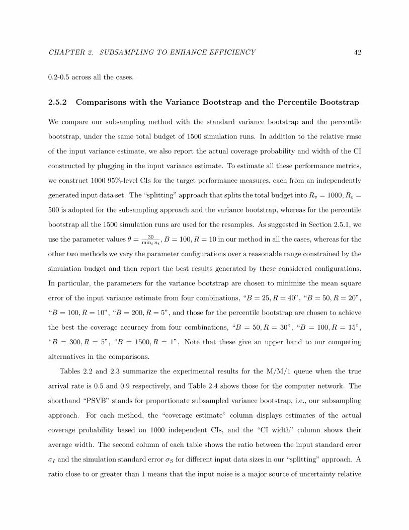
CHAPTER 2. SUBSAMPLING TO ENHANCE EFFICIENCY 42
0.2-0.5 across all the cases.
2.5.2 Comparisons with the Variance Bootstrap and the Percentile Bootstrap
We compare our subsampling method with the standard variance bootstrap and the percentile
bootstrap, under the same total budget of 1500 simulation runs. In addition to the relative rmse
of the input variance estimate, we also report the actual coverage probability and width of the CI
constructed by plugging in the input variance estimate. To estimate all these performance metrics,
we construct 1000 95%-level CIs for the target performance measures, each from an independently
generated input data set. The “splitting” approach that splits the total budget intoRv = 1000, Re =
500 is adopted for the subsampling approach and the variance bootstrap, whereas for the percentile
bootstrap all the 1500 simulation runs are used for the resamples. As suggested in Section 2.5.1, we
use the parameter values θ = 30mini ni
, B = 100, R = 10 in our method in all the cases, whereas for the
other two methods we vary the parameter configurations over a reasonable range constrained by the
simulation budget and then report the best results generated by these considered configurations.
In particular, the parameters for the variance bootstrap are chosen to minimize the mean square
error of the input variance estimate from four combinations, “B = 25, R = 40”, “B = 50, R = 20”,
“B = 100, R = 10”, “B = 200, R = 5”, and those for the percentile bootstrap are chosen to achieve
the best the coverage accuracy from four combinations, “B = 50, R = 30”, “B = 100, R = 15”,
“B = 300, R = 5”, “B = 1500, R = 1”. Note that these give an upper hand to our competing
alternatives in the comparisons.
Tables 2.2 and 2.3 summarize the experimental results for the M/M/1 queue when the true
arrival rate is 0.5 and 0.9 respectively, and Table 2.4 shows those for the computer network. The
shorthand “PSVB” stands for proportionate subsampled variance bootstrap, i.e., our subsampling
approach. For each method, the “coverage estimate” column displays estimates of the actual
coverage probability based on 1000 independent CIs, and the “CI width” column shows their
average width. The second column of each table shows the ratio between the input standard error
σI and the simulation standard error σS for different input data sizes in our “splitting” approach. A
ratio close to or greater than 1 means that the input noise is a major source of uncertainty relative

CHAPTER 2. SUBSAMPLING TO ENHANCE EFFICIENCY 43
to the simulation noise, thus indicating the need to be taken into account in output analysis.
mini niσIσS
PSVB variance bootstrap percentile bootstraprelativermse
coverageestimate
CI widthrelativermse
coverageestimate
CI widthcoverageestimate
CI width
30 7.74 0.73 84.3% 0.422 0.73 84.3% 0.422 91.9% 0.467100 3.77 0.55 92.5% 0.251 0.80 88.6% 0.248 98.8% 0.356300 2.13 0.44 94.8% 0.156 1.04 85.6% 0.148 99.9% 0.3071000 1.15 0.38 95.0% 0.103 2.48 89.4% 0.111 100% 0.2852000 0.79 0.38 95.9% 0.087 5.43 92.8% 0.107 100% 0.280
Table 2.2: Results for the M/M/1 queue with arrival rate 0.5 and service rate 1.
mini niσIσS
PSVB variance bootstrap percentile bootstraprelativermse
coverageestimate
CI widthrelativermse
coverageestimate
CI widthcoverageestimate
CI width
30 11.12 0.59 81.4% 0.609 0.59 81.4% 0.609 94.6% 0.639100 6.22 0.42 89.9% 0.372 0.63 88.6% 0.386 97.2% 0.446300 3.46 0.32 92.6% 0.225 0.71 87.0% 0.225 99.3% 0.3481000 1.86 0.27 93.3% 0.137 1.21 86.3% 0.137 100% 0.3072000 1.30 0.24 95.0% 0.108 2.19 90.7% 0.119 100% 0.2944000 0.91 0.23 94.9% 0.089 3.61 91.2% 0.106 100% 0.288
Table 2.3: Results for the M/M/1 queue with arrival rate 0.9 and service rate 1.
mini niσIσS
PSVB variance bootstrap percentile bootstraprelativermse
coverageestimate
CI width(×10−4)
relativermse
coverageestimate
CI width(×10−4)
coverageestimate
CI width(×10−4)
30 12.60 0.74 92.0% 19.3 0.74 92.0% 19.3 95.2% 22.0150 5.36 0.41 94.3% 8.85 0.53 91.3% 8.50 98.3% 11.2750 2.35 0.32 94.2% 4.27 0.94 86.9% 3.88 100% 7.971800 1.53 0.28 95.3% 3.03 1.63 87.1% 3.01 100% 7.34
Table 2.4: Results for the computer network.
We compare the approaches based on Tables 2.2-2.4. Firstly, our subsampling approach signif-
icantly outperforms the variance bootstrap in terms of estimation accuracy of the input variance.
The estimates generated by our approach have a smaller relative error than those by the variance
bootstrap in all considered cases, and the gap becomes more significant as the data size grows
larger. In particular, as the data size grows from 30 to thousands, the estimation error keeps de-
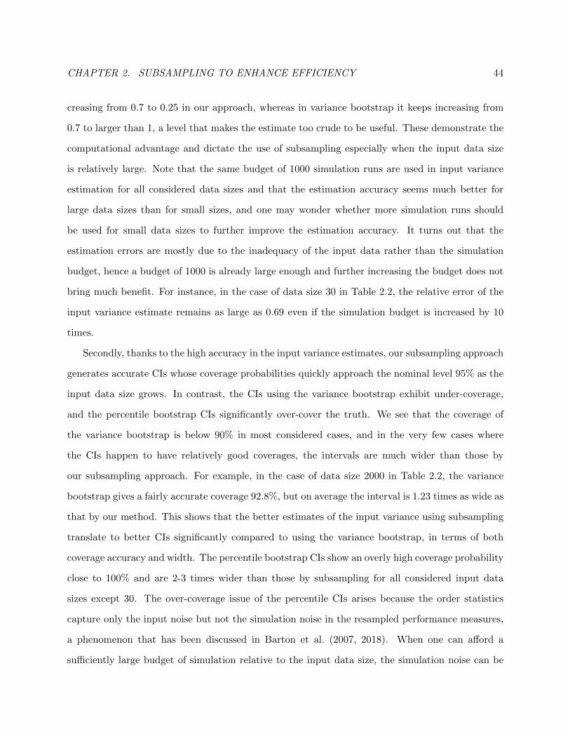
CHAPTER 2. SUBSAMPLING TO ENHANCE EFFICIENCY 44
creasing from 0.7 to 0.25 in our approach, whereas in variance bootstrap it keeps increasing from
0.7 to larger than 1, a level that makes the estimate too crude to be useful. These demonstrate the
computational advantage and dictate the use of subsampling especially when the input data size
is relatively large. Note that the same budget of 1000 simulation runs are used in input variance
estimation for all considered data sizes and that the estimation accuracy seems much better for
large data sizes than for small sizes, and one may wonder whether more simulation runs should
be used for small data sizes to further improve the estimation accuracy. It turns out that the
estimation errors are mostly due to the inadequacy of the input data rather than the simulation
budget, hence a budget of 1000 is already large enough and further increasing the budget does not
bring much benefit. For instance, in the case of data size 30 in Table 2.2, the relative error of the
input variance estimate remains as large as 0.69 even if the simulation budget is increased by 10
times.
Secondly, thanks to the high accuracy in the input variance estimates, our subsampling approach
generates accurate CIs whose coverage probabilities quickly approach the nominal level 95% as the
input data size grows. In contrast, the CIs using the variance bootstrap exhibit under-coverage,
and the percentile bootstrap CIs significantly over-cover the truth. We see that the coverage of
the variance bootstrap is below 90% in most considered cases, and in the very few cases where
the CIs happen to have relatively good coverages, the intervals are much wider than those by
our subsampling approach. For example, in the case of data size 2000 in Table 2.2, the variance
bootstrap gives a fairly accurate coverage 92.8%, but on average the interval is 1.23 times as wide as
that by our method. This shows that the better estimates of the input variance using subsampling
translate to better CIs significantly compared to using the variance bootstrap, in terms of both
coverage accuracy and width. The percentile bootstrap CIs show an overly high coverage probability
close to 100% and are 2-3 times wider than those by subsampling for all considered input data
sizes except 30. The over-coverage issue of the percentile CIs arises because the order statistics
capture only the input noise but not the simulation noise in the resampled performance measures,
a phenomenon that has been discussed in Barton et al. (2007, 2018). When one can afford a
sufficiently large budget of simulation relative to the input data size, the simulation noise can be

CHAPTER 2. SUBSAMPLING TO ENHANCE EFFICIENCY 45
made negligible so that the CIs have the correct coverage. However, when simulation resources are
relatively limited (e.g., when data size≥ 100 in Tables 2.2-2.4), the CIs are unnecessarily widened by
the extra simulation noise that leads to over-coverage. We also notice that the percentile bootstrap
CIs do show more accurate coverage than the other two methods when the input data size is 30,
which may suggest that the percentile bootstrap is the preferred approach to constructing CIs in
small data cases. However, this outperformance is a result of optimally choosing the parameters
B,R in hindsight. In our experiments, this best parameter set varies from one case to another, and
the actual coverage under different configurations varies in a range of 8%.
Thirdly, results across different input data sizes show that, the advantages of subsampling in
both input variance estimation and CI construction are most significant in situations with relatively
large input data size. Note that one may argue in such situations input uncertainty is negligible.
However, whether this is indeed the case relates to the error tolerance of the decision-maker and the
magnitude of the target performance measure itself. For the large data sizes we consider, the input
noise appears still relatively substantial. For instance, when the input data size is 2000 in Table
2.3, the average width of the CIs as a measure of the input uncertainty and simulation uncertainty
combined amounts to as much as 57% of the target tail probability, and that the input uncertainty
serves as a major component of the total uncertainty (a ratio of 1.3 relative to the simulation
uncertainty).
Lastly, in situations with small input data size like 30 the CI coverage clearly falls below 95% in
Tables 2.2 and 2.3. This under-coverage phenomenon may appear to stem from the nonlinear effect
of the performance measure that is inadequately captured by the Gaussian-approximation-based
CI given in (2.3). The real reason, as our experiments suggest, turns out to be the insufficient
accuracy of the input variance estimates. In fact, if the true input variance σ2I (which can be
accurately estimated by repeatedly generating independent input data sets) is plugged into (2.3)
to construct CIs, the coverage probability under the data size 30 rises to 94%-95% for both the
M/M/1 queue and the computer network. This indicates a positive impact of an accurate input
variance estimate on the CI quality, a point that we will discuss further momentarily.

CHAPTER 2. SUBSAMPLING TO ENHANCE EFFICIENCY 46
2.5.3 Constructing CI via Input Variance and Comparisons of the Splitting and
Nonsplitting Approaches
We study in more depth the relation between the input variance estimation accuracy and CI quality,
and compare the splitting approach for CI construction that has been used in previous subsections,
with the alternate nonsplitting approach described at the beginning of this section. Finally, we
provide practical budget allocation strategies for the splitting approach.
First, to see how the estimation accuracy of the input variance affects the coverage accuracy
of the CIs, we use the splitting approach to compute 95%-level CIs, with 1000 simulation runs
assigned to input variance estimation and another 500 runs to point estimator evaluation. Figure
2.4a plots the coverage probability versus the relative rmse when the subsample size θmini ni is
chosen 30 in the M/M/1 queue example, where each point corresponds to a particular combination
of the data size mini ni, the outer replication size B, and the inner replication size R. Figure 2.4b
plots the same for the computer network example with subsample size 30. Both figures clearly
show that, the more accurately the input variance is estimated, the closer to the nominal level 95%
the coverage probability will be. Accurate estimation of the input variance thus appears to play a
crucial role in the construction of accurate CIs.
0.35 0.4 0.45 0.5 0.55 0.6 0.65 0.7 0.75 0.8 0.85
relative rmse of input variance estimate
84
86
88
90
92
94
96
co
ve
rag
e p
rob
ab
ility
(%
)
(a) M/M/1 queue with arrival rate 0.5, θmini ni = 30.
0.2 0.3 0.4 0.5 0.6 0.7 0.8 0.9 1 1.1
relative rmse of input variance estimate
91
91.5
92
92.5
93
93.5
94
94.5
95
95.5
96
co
ve
rag
e p
rob
ab
ility
(%
)
(b) Computer network, θmini ni = 30.
Figure 2.4: Monotonicity between coverage accuracy and input variance estimation accuracy.
Next we compare the splitting and nonsplitting approaches under the same total budget of
1500 simulation runs. Like in the splitting approach, we use a subsample size θmini ni = 30 for
our nonsplitting approach, but use B = 75, B = 20 to consume all the 1500 simulation runs. We

CHAPTER 2. SUBSAMPLING TO ENHANCE EFFICIENCY 47
find that the CIs generated from the two approaches have similar lengths, but the nonsplitting
approach underperforms in terms of coverage accuracy. Each plot in Figure 2.5 shows the coverage
probabilities of the nonsplitting CIs versus the splitting ones for each of the considered example
systems, as the input data size grows from 30 to thousands. We see that when the data size is
relatively small (e.g., below 500), the two approaches generate CIs with similar coverage accuracy.
When the data size grows larger, however, the coverage probability of the nonsplitting CIs keeps
dropping in all the three examples, especially in the M/M/1 queue with arrival rate 0.9 where
a drop towards 86% is observed, whereas the splitting CIs exhibit almost exact 95% coverage.
A possible cause of the undercoverage is the overly small subsample size compared to the input
data size, which leads to a high bias in the point estimator. With a subsample size s, the bias of
the nonsplitting point estimator E∗[ψ] with respect to the truth ψ(F1, . . . , Fm) can be as large as
O(1/s). Given that the input standard error is Θ(1/√n), E∗[ψ] has a negligible bias only when
the subsample size is large enough, namely when s = ω(√n), indicating that a small subsample
size relative to the data size can corrupt the CI. In our experiment, we find that the (supposedly
unobservable) bias can be as large as 25% of the CI width when the input data size is 2000 in the
M/M/1 queue with arrival rate 0.9, and that artificially removing the bias from the point estimator
can improve the coverage to a similar level achieved by the splitting approach. Because of the bias
and the consequent under-coverage issue, we caution the use of the non-splitting approach, that it
should only be used when a relatively large subsample size is adopted.
Since the splitting approach is recommended, next we explore strategies of splitting a given
budget. Our goal is to generate shortest possible CIs that have a sufficiently accurate coverage
probability. As in the beginning of the section, denote by Rv the number of simulation runs used to
estimate the input variance, and by Re to construct the point estimator. Under a fixed total budget
Rv +Re = 1500, we try four different splits Rv = 100, 250, 500, 1000 (accordingly Re = 1500−Rv),
and for each split the subsample size is fixed at θmini ni = 30 and several choices of B,R are tested
among which the one with the best coverage probability is reported. Figure 2.6 plots the coverage
probability versus the CI width for the four considered splits, where the M/M/1 queue with arrival
rate 0.9 is considered and input data size is 2000. We notice that the split controls a tradeoff

CHAPTER 2. SUBSAMPLING TO ENHANCE EFFICIENCY 48
0 200 400 600 800 1000 1200 1400 1600 1800 2000
minin
i
84
86
88
90
92
94
96co
ve
rag
e p
rob
ab
ility
(%
)
nominal level 95%
nonsplit
split
(a) M/M/1 queue with arrival rate 0.5.
0 500 1000 1500 2000 2500 3000 3500 4000
minin
i
82
84
86
88
90
92
94
96
co
ve
rag
e p
rob
ab
ility
(%
)
nominal level 95%
nonsplit
split
(b) M/M/1 queue with arrival rate 0.9.
0 200 400 600 800 1000 1200 1400 1600 1800 2000
minin
i
91
91.5
92
92.5
93
93.5
94
94.5
95
95.5
96
cove
rag
e p
rob
ab
ility
(%
)
nominal level 95%
nonsplit
split
(c) Computer network.
Figure 2.5: Coverage comparison under the splitting and nonsplitting approaches.
between the coverage accuracy and the CI width. The more simulation runs one allocates to input
variance estimation, the more accurate but wider CIs one would obtain, because the input variance
is more accurately estimated while the point estimator becomes more noisy. The plot suggests
that allocating 500-1000 replications to variance estimation achieves a good balance of accuracy
and width, in the sense that the intervals from the split “500+1000” or “1000 + 500” are only
slightly wider than those by other splits and that allocating less (say 250) to variance estimation
results in a considerable drop in coverage probability from the nominal level 95%. The results
from Tables 2.2-2.4, where the split “1000 + 500” is used, also validates the effectiveness of such a
strategy. Therefore, for a given simulation budget, we recommend that the user allocate 500-1000
replications to input variance estimation with our subsampling approach and all the remaining
budget to the construction of the point estimator.

CHAPTER 2. SUBSAMPLING TO ENHANCE EFFICIENCY 49
0.08 0.085 0.09 0.095 0.1 0.105 0.11 0.115 0.12
average CI width
86
88
90
92
94
96
co
ve
rag
e p
rob
ab
ility
(%
)
100 + 1400
250 + 1250
500 + 1000
1000 + 500
Figure 2.6: Coverage probability versus CI width, under different budget splits in the form of“Rv +Re”.
2.6 Conclusion
We have explained how estimating input variances in stochastic simulation can require large com-
putation effort when using conventional bootstrapping. This arises as the bootstrap involves a
two-layer sampling, which adds up to a total effort of larger order than the data size in order to
achieve relative consistency. To alleviate this issue, we have proposed a subsampling method that
leverages the relation between the structure of input variance and the estimation error from the
two-layer sampling, so that the resulting total effort can be reduced to being independent of the
data size. We have presented the theoretical results in this effort reduction, and the optimal choices
of the subsample ratio and simulation budget allocation in terms of the data size and the budget.
We have also demonstrated numerical results to support our theoretical findings, and provided
guidelines in using our proposed methods to estimate input variances and also construct output
CIs.

CHAPTER 3. OPTIMIZATION-BASED QUANTIFICATION 50
Chapter 3
Optimization-Based Quantification of
Simulation Input Uncertainty via
Empirical Likelihood
3.1 Introduction
Following Chapter 2, we continue investigating input uncertainty quantification in this chapter,
but switch focus from input variance estimation to the construction of CIs for simulation outputs
that account for input uncertainty in addition to the noises in generating the random variates in
the simulation process. Again we focus particularly on the nonparametric regime. A common
approach is the bootstrap (e.g., Barton and Schruben 1993, 2001), which repeatedly generates
resampled distributions to drive simulation runs and uses the quantiles of the simulated outputs to
construct the CIs. Another approach is the delta method (e.g., Asmussen and Glynn 2007, Chapter
III) that estimates the asymptotic variance in the central limit theorem (CLT) directly. The latter
has been considered mostly in the parametric setting (e.g., Cheng and Holland 1997, 1998, 2004)
but bears a straightforward analog in our considered nonparametric scenario (as has been discussed
in Section 2.2.2). Estimating this variance can also be conducted by subsampling (i.e.,Chapter 2)
or bootstrapping (e.g., Cheng and Holland 1997, Song and Nelson 2015).

CHAPTER 3. OPTIMIZATION-BASED QUANTIFICATION 51
Our focus in this chapter is a new approach to construct input-induced CIs by using optimization
as an underpinning tool. Our approach looks for a set of “maximal” and a set of “minimal”
probability weights on the input data, obtained by solving a pair of convex optimization problems
with constraints involving a suitably averaged statistical divergence. These weights can be viewed
as “worst-case” representations of the input distributions which are then used to generate the input
variates to drive the simulation, giving rise to upper and lower bounds that together form a CI on
the performance measure of interest.
We will illustrate how this optimization-based approach offers benefits relative to the bootstrap
and the delta method. The bootstrap typically involves nested simulation due to the resampling
step before simulation runs, which leads to a multiplicative computational requirement. Its perfor-
mance can be sensitive to the simulation budget size and allocation rule in the nested procedure. A
key element of our approach is to use convex optimization to replace the resampling step, which by-
passes the multiplicative budget allocation problem and gives more robust performances, especially
under small input data sizes. On the other hand, the overhead in setting up our optimization is more
substantial than the bootstrap when the input data size is large. It should be noted that the boot-
strap possesses more flexibility as the resampled simulation replications can be used to approximate
many statistics and to construct CIs at different confidence levels, without re-running the bootstrap
procedure again. On the contrary, our approach needs re-optimization and a re-evaluation step for
each new confidence level or statistic of interest. Nonetheless, the monotonicity structure of our
decision space in the target confidence level allows us to speed up the re-optimization by starting
the optimization for a high confidence level at the solution obtained for a low confidence level, while
the re-evaluation step only requires a sample size for standard output analysis that is free of input
uncertainty.
Our method is closer to the delta method than the bootstrap in that, like the former, we need to
estimate gradient information. While our approach and the delta method have similar asymptotic
behaviors, we will demonstrate how our approach tends to outperform in finite sample. Roughly
speaking, this outperformance arises since the delta method relies heavily on a linear approximation
in constructing CIs. When the standard error, which arises from this linear approximation, is noisily

CHAPTER 3. OPTIMIZATION-BASED QUANTIFICATION 52
estimated, the resulting CI tends to exhibit under-coverage issues. In contrast, using the weighted
distributions to drive simulation runs in our approach is less sensitive to the quality of the standard
error estimation, and moreover can introduce nonlinearity that naturally follows the boundaries of
a given problem, which in turn alleviates the under-coverage issue experienced in the delta method.
As our main technical contributions, we design and analyze procedures to achieve tight statistical
coverage guarantees for the resulting optimization-based CIs. Our approach aligns with the recent
surge of robust optimization (Ben-Tal and Nemirovski 2002, Bertsimas et al. 2011) in handling
decision-making under uncertainty, where decisions are chosen to perform well under the worst-case
scenario among a so-called uncertainty or ambiguity set of possibilities. Our approach particularly
resembles distributionally robust optimization (DRO) (e.g., Ben-Tal et al. 2013, Delage and Ye
2010, Goh and Sim 2010, Wiesemann et al. 2014) where the uncertainty of the considered problem
lies in the probability distributions, as our involved optimization formulation contains decision
variables that are probability weights of the input distributions. However, contrary to the DRO
rationale that postulates the uncertainty sets to contain the truth (including those studied recently
in the simulation literature; Hu et al. 2012, Glasserman and Xu 2014, Lam 2016b, 2018, Ghosh
and Lam 2019), we will explain our procedures by viewing the constraints as log-likelihoods on the
input data, and develop the resulting statistical guarantees from a multi-sample generalization of the
empirical likelihood (EL) method (Owen 2001), a nonparametric analog of the celebrated maximum
likelihood method in parametric statistics. Consequently, the form of our proposed constraint (i.e.,
the averaged statistical divergence constraint) differs drastically from previous DRO suggestions,
and the guarantee is provably tight asymptotically. We mention that, though EL has appeared in
statistics for a long time, its use in operations research has appeared only recently and is limited
to optimization problems (e.g., Lam and Zhou 2017, Duchi et al. 2016, Lam 2019, Blanchet and
Kang 2020, Blanchet et al. 2019). We therefore contribute by showing that a judicious use of this
idea can offer new benefits in the equally important area of simulation analysis.
The rest of this chapter is as follows. Section 3.2 reviews some related literature. Section
3.3 presents our procedure and main results on statistical guarantees. Section 3.4 explains the
underlying theory giving rise to our approach and statistical results. Section 3.5 shows some

CHAPTER 3. OPTIMIZATION-BASED QUANTIFICATION 53
numerical results and compares with previous approaches. All technical proofs are left to Appendix
B.
3.2 Related Literature
A review on the problem of input uncertainty has been given in Chapter 2, therefore here we
briefly survey two methodologically related areas. Our methodologies are related to several tools
in statistics. First is the EL method. Initially proposed by Owen (1988) as a nonparametric
counterpart of the maximum likelihood theory, the EL method has been widely studied in statistical
problems like regression and hypothesis testing etc. (e.g., Qin and Lawless 1994, Owen 2001, Hjort
et al. 2009). Its use in operations research is relatively recent and is limited to optimization.
Lam and Zhou (2017) investigates the use of EL in quantifying uncertainty in sample average
approximation. Lam (2019) uses EL to derive uncertainty sets for DRO that guarantees feasibility
for stochastic constraints. Duchi et al. (2016) generalizes the EL method to Hadamard differentiable
functions and obtains tight optimality bounds for stochastic optimization problems. Blanchet and
Kang (2020), Blanchet et al. (2019) generalize the EL method to inference using the Wasserstein
distance. In addition, our work also utilizes the influence function, which captures nonparametric
sensitivity information of a statistic, and is first proposed by Hampel (1974) in the context of robust
statistics (Huber and Ronchetti 2009, Hampel et al. 2011) as a heuristic tool to measure the effect
of data contamination. Influence function is also used in deriving asymptotic results for von Mises
differentiable functionals which have profound applications in U -statistics (Serfling 2009).
Our approach resembles DRO, which utilizes worst-case perspectives in stochastic decision-
making problems under ambiguous probability distributions. In particular, our optimization posited
over the space of input probability distributions has a similar spirit as the search for the worst-case
distribution in the inner optimization in DRO. The DRO framework has been applied in various
disciplines such as economics (Hansen and Sargent 2008), finance (Glasserman and Xu 2013, 2014),
stochastic control (Petersen et al. 2000, Iyengar 2005, Nilim and El Ghaoui 2005, Xu and Mannor
2012), queueing (Jain et al. 2010) and dynamic pricing (Lim and Shanthikumar 2007). Among

CHAPTER 3. OPTIMIZATION-BASED QUANTIFICATION 54
them, constraints in terms of φ-divergences, which include the Burg-entropy divergence appearing
in our approach, have been considered in, e.g. Ben-Tal et al. (2013), Bayraksan and Love (2015),
Jiang and Guan (2016), so are other types of statistical distances such as Renyi divergence (e.g.,
Atar et al. 2015, Dey and Juneja 2012, Blanchet et al. 2020) and the Wasserstein distance (e.g.,
Esfahani and Kuhn 2018, Blanchet and Murthy 2019, Gao and Kleywegt 2016), and other constraint
types including moments and support (e.g., Delage and Ye 2010, Goh and Sim 2010, Hu et al. 2012,
Wiesemann et al. 2014). In simulation, the DRO idea has appeared in Glasserman and Xu (2014),
Lam (2016b, 2018), Ghosh and Lam (2019) in quantifying model risks. Nonetheless, although
our involved optimization looks similar to DRO, the underpinning statistical guarantees of our
approach stem from the EL method. As we will explain, our constraints possess properties that are
dramatically different from those studied in DRO, and their precise forms also deviate from any
known DRO suggestions.
3.3 Optimization-Based Confidence Intervals
This section presents our main procedure and statistical guarantees. We start with our problem
setting and some notations.
3.3.1 Problem Setting
We consider a performance measure in the form
Z∗ = Z(P1, . . . , Pm) = EP1,...,Pm [h(X1, . . . ,Xm)] , (3.1)
where P1, . . . , Pm are m independent input models, Xi = (Xi(1), . . . , Xi(Ti)) is a sequence of Ti
i.i.d. input variates each distributed under Pi, and Ti is a deterministic run length. The distribution
Pi has (possibly multivariate) domain Xi. The function h mapping from XT11 × · · · × XTmm to R is
assumed computable given the inputs Xi. In other words, given the sequence X1, . . . ,Xm, the value
of h(X1, . . . ,Xm) can be evaluated by the computer. The notation EP1,...,Pm [·] is a shorthand for
EPT11 ×···×P
Tmm
[·], the expectation taken over all the independent i.i.d. sequences X1, . . . ,Xm, i.e.,

CHAPTER 3. OPTIMIZATION-BASED QUANTIFICATION 55
under the product measure P T11 ×· · ·×P Tmm . We use Xi to denote a generic random variable/vector
distributed under Pi.
As a simple example, X1 and X2 can represent respectively the sequences of inter-arrival times
and service times in a queueing system. P1 and P2 represent the corresponding input distributions.
h denotes the indicator function of the exceedance of some waiting time above a threshold. Then
Z(P1, P2) becomes the waiting time tail probability.
Our premise is that there exists a true Pi that is unknown for each i, but a sample of ni
i.i.d. observations Xi,1, . . . , Xi,ni is available from each Pi. The true value of (3.1) is therefore
unknown even under abundant simulation runs. Our goal is to find an asymptotically accurate
(1−α)-level CI for the true performance measure Z∗. To be more precise, we call a CI asymptotically
exact if it consists of two numbers L ,U , derived from the data and the simulation, such that
limeach ni andR→∞
P (L ≤ Z∗ ≤ U ) = 1− α
where R is the total number of simulation replications involved in generating the CI, and the
probability P is taken with respect to the joint randomness in the data and the simulation. The
asymptotic above is qualified by certain growth rates of ni and R that we will detail.
Along our development will also arise cases in which a coverage guarantee is provided as a lower
bound, i.e.,
lim infeach ni andR→∞
P (L ≤ Z∗ ≤ U ) ≥ 1− α
We call [L ,U ] an asymptotically valid (1− α)-level CI. The CIs constructed from our procedures
will be either asymptotically exact or, asymptotically valid and accompanied with an associated
upper bound that quantities the tightness of the coverage. Lastly, our developments fix the number
of independent input models m and the run lengths Ti’s, i.e., we focus primarily on transient
performance measures with a moderate number of input models relative to the data and simulation
sizes.

CHAPTER 3. OPTIMIZATION-BASED QUANTIFICATION 56
3.3.2 Main Procedure
Algorithm 4 gives a step-by-step description of our basic procedure for computing L and U . The
quantity ˆGi(Xi,j) for each i = 1, . . . ,m, j = 1, . . . , ni introduced in Step 1 is the sample estimate of
the so-called influence function of Z, which can be viewed as the gradient of Z taken with respect to
the input distributions (see Assumption 3.3.2 and the subsequent discussion). This sample estimate
of the influence function is obtained from R1 simulation runs. The same simulation replications are
also used to compute an estimate Z(P1, . . . , Pm) of the performance measure under the empirical
input models, that is, each Pi(·) = 1ni
∑nij=1 δXi,j (·) where δXi,j (·) denotes the delta measure on
Xi,j .
Step 2 in Algorithm 4 outputs a minimizer and a maximizer of the optimization (3.3) in which
“min /max” denotes a pair of minimization and maximization, and the calibrating constant X 21,1−α
is the 1−α quantile of the chi-square distribution with degree of freedom one. Optimization (3.3) can
be viewed as a sample average approximation (SAA) (Shapiro et al. 2014) on the influence function
(expressible as an expectation), with decision variables being the probability weights wi,j , i =
1, . . . ,m, j = 1, . . . , ni on the influence function evaluated at each observation Xi,j of input model
i. For convenience, we denote wi = (wi,j)j=1,...,ni as the weight vector associated with input model
i, and w = (wi)i=1,...,m be the aggregate weight vector.
Optimization (3.3) can be interpreted as two worst-case optimization problems over m indepen-
dent input distributions, each on support Xi,1, . . . , Xi,ni, subject to a weighted average of individ-
ual statistical divergences (Pardo 2005). To explain, the quantity Dni(wi) = − 1ni
∑nij=1 log(niwi,j)
is the Burg-entropy divergence (Ben-Tal et al. 2013) (or the Kullback-Leibler (KL) divergence)
between the probability weights wi and the uniform weights. Thus, letting N =∑m
i=1 ni be the
total number of observations from all input models, we have
− 1
N
m∑i=1
ni∑j=1
log(niwi,j) =m∑i=1
niN
− 1
ni
ni∑j=1
log(niwi,j)
=m∑i=1
niNDni(wi)
which is an average of the Burg-entropy divergences imposed on different input models, each
weighted by the proportion of the respective observations, ni/N . The first constraint in (3.3)

CHAPTER 3. OPTIMIZATION-BASED QUANTIFICATION 57
Algorithm 4 Basic Empirical-Likelihood-Based Procedure (BEL)
Input: Data Xi,1, . . . , Xi,ni for each input model i = 1, . . . ,m. A target confidence level 1− α,
and numbers of simulation replications, R1, 2R2, to be used in Step 1 and Step 3 respectively.
Procedure:
1. Influence Function Estimation: For each i = 1, . . . ,m, j = 1, . . . , ni compute estimate of
the influence function evaluated at Xi,j
ˆGi(Xi,j) =1
R1
R1∑r=1
[(h(Xr
1, . . . ,Xrm)− Z(P1, . . . , Pm))(ni
Ti∑t=1
1Xri (t) = Xi,j − Ti)
](3.2)
where for each r = 1, . . . , R1, Xri = (Xr
i (1), . . . , Xri (Ti)) are i.i.d. variates drawn independently
from the uniform distribution on Xi,1, . . . , Xi,ni for each i, 1· is the indicator function, and
Z(P1, . . . , Pm) =∑R1
r=1 h(Xr1, . . . ,X
rm)/R1 is the sample mean of the outputs.
2. Optimization: Compute respective optimal solutions (wmin1 , . . . ,wmin
m ) and
(wmax1 , . . . ,wmax
m ) of the following pair of programs
min /maxm∑i=1
ni∑j=1
ˆGi(Xi,j)wi,j
subject to − 2m∑i=1
ni∑j=1
log(niwi,j) ≤ X 21,1−α
ni∑j=1
wi,j = 1, for all i = 1, . . . ,m
wi,j ≥ 0, for all i = 1, . . . ,m, j = 1, . . . , ni.
(3.3)
3. Evaluation: Compute
L BEL =1
R2
R2∑r=1
h(Xr,min1 , . . . ,Xr,min
m ), U BEL =1
R2
R2∑r=1
h(Xr,max1 , . . . ,Xr,max
m )
where for each r = 1, . . . , R2, Xr,mini = (Xr,min
i (1), . . . , Xr,mini (Ti)) and Xr,max
i =
(Xr,maxi (1), . . . , Xr,max
i (Ti)) are i.i.d. variates drawn independently from a weighted distribution
on Xi,1, . . . , Xi,ni, according to weights wmini and wmax
i , respectively for each i.
Output: The CI [L BEL,U BEL].

CHAPTER 3. OPTIMIZATION-BASED QUANTIFICATION 58
can thus be written asm∑i=1
niNDni(wi) ≤
X 21,1−α2N
which constitutes a neighborhood ball of size X 21,1−α/(2N) measured by the averaged Burg-entropy
divergence.
Finally, Step 3 in Algorithm 4 uses the obtained optimal probability weights wmini and wmax
i
to form two weighted empirical distributions on Xi,jj=1,...,ni for input model i, which are used
to drive two independent sets of simulation runs, each of size R2, in order to output the lower and
upper confidence bounds respectively.
An efficient method to solve optimization (3.3) is discussed in the following proposition:
Proposition 3.3.1 For each i and every β > 0 define λi(β) to be the unique solution of the
equationni∑j=1
2β
ˆGi(Xi,j) + λi= 1 (3.4)
on the interval (−minjˆGi(Xi,j),∞). Let β∗ > 0 solve the equation
2
m∑i=1
ni∑j=1
log2niβ
ˆGi(Xi,j) + λi(β)+ X 2
1,1−α = 0. (3.5)
If there exist some i0 ∈ 1, . . . ,m and j1, j2 ∈ 1, . . . , ni0 such that ˆGi0(Xi0,j1) 6= ˆGi0(Xi0,j2),
then β∗ ∈(0, D/
(2(1 − e−
X21,1−α2N
)mini ni
))and is unique, where D = maxmaxj
ˆGi(Xi,j) −
minjˆGi(Xi,j)|i = 1, . . . ,m, N =
∑mi=1 ni, and the minimizer (wmin
1 , . . . ,wminm ) of (3.3) can be
obtained by
wmini,j =
2β∗
ˆGi(Xi,j) + λi(β∗).
The maximizer (wmax1 , . . . ,wmax
m ) can be computed in the same way except that each ˆGi(Xi,j) is
replaced by − ˆGi(Xi,j).
Otherwise, if for each i = 1, . . . ,m the coefficient ˆGi(Xi,j) takes the same value across all
j = 1, . . . , ni, then (3.3) has a constant objective hence becomes trivial. In this case, one can
output (wmin1 , . . . ,wmin
m ) and (wmax1 , . . . ,wmax
m ) as any solution in the feasible set (e.g., the uniform

CHAPTER 3. OPTIMIZATION-BASED QUANTIFICATION 59
weights, i.e., wmaxi,j = wmin
i,j = 1/ni for all i, j).
The proof of Proposition 3.3.1 uses the Karush-Kuhn-Tucker (KKT) conditions of (3.3), and can
be found in Section B.7 of the Appendix. To implement what Proposition 3.3.1 suggests, we first
check whether ˆGi(Xi,j1) 6= ˆGi(Xi,j2) for some i = 1, . . . ,m and some 1 ≤ j1 < j2 ≤ ni, in which case
the maximizer (wmax1 , . . . ,wmax
m ) and minimizer (wmin1 , . . . ,wmin
m ) of (3.3) are unique. Here, given
a value of β we can efficiently evaluate each λi(β) by solving (3.4) with Newton’s method. Then, β∗
is obtained by running a bisection on (3.5) over the interval (0, D/(2(1−e−
X21,1−α2N
)mini ni
))whose
convergence is guaranteed by the uniqueness of β∗ and the continuity of (3.5) in β, and finally each
wmini,j or wmax
i,j is computed from β∗, λi(β∗)’s and ˆGi(Xi,j)’s. Note that for any β > 0 the left hand
side of (3.4) is monotonically decreasing and convex in λi, hence Newton’s method is guaranteed to
converge to λi(β) as long as it starts within (−minjˆGi(Xi,j), λi(β)), say at 2β−minj
ˆGi(Xi,j). The
advantage of this approach over directly solving the convex optimization (3.3) is that we reduce the
dimension of the decision space, from linear in the sample sizes to only solving univariate equations
in (3.4) and (3.5), which is much more favorable when the sample sizes are large. Finally, note that
if ˆGi(Xi,j1) = ˆGi(Xi,j2) for all i = 1, . . . ,m and all 1 ≤ j1 < j2 ≤ ni, then, as the objective function
of (3.3) becomes a constant, we can take any solution in the feasible set; for concreteness we can
take (wmin1 , . . . ,wmin
m ) and (wmax1 , . . . ,wmax
m ) to be the uniform weights.
Next we provide two variants of Algorithm 4, depicted as Algorithms 5 and 6, which differ only
by the last step. The motivation (with more details in Section 3.4.6) is that Algorithm 4 tends
to under-cover the true performance value because its last step only outputs the sample mean of
the simulation replications and does not take full account of the stochastic uncertainty. Algorithm
5 takes care of this uncertainty by outputting the standard normal lower and upper confidence
bounds in the last step. However, this simple adjustment does not account for the joint variances
from the input data and the stochasticity in a tight manner, and tends to generate conservative CIs
that over-cover the truth. This motivates the refined adjustment in Algorithm 6 that is designed to
match the CI inflation from combined input and stochastic uncertainties, by taking into account the
asymptotic form of the joint variance, and subsequently leads to accurate coverage performances.
To explain intuitively, with no simulation noise, an asymptotically exact CI under input uncertainty

CHAPTER 3. OPTIMIZATION-BASED QUANTIFICATION 60
would output a point estimate of the target performance measure plus or minus a standard error of
magnitude z1−α/2σI , where σ2I denotes the input-induced variance. As we will develop in Section
3.4, using the weights (wmin1 , . . . ,wmin
m ) and (wmax1 , . . . ,wmax
m ) on Xi,1, . . . , Xi,ni, i = 1, . . . ,m,
obtained in Step 2 of the algorithms, to evaluate the performance measure essentially matches this
CI as long as no simulation noise is present in the evaluation step. When R2 is finite, however,
the standard error should be inflated to z1−α/2
√σ2I + σ2/R2 where σ2 denotes the variance of one
simulation run. But as z1−α/2σI is already implicitly elicited by the optimal weights, it needs to
be removed from this standard error to avoid over-coverage. This leads to the adjustment in Step
3 of Algorithm 6, where σ2I is an estimate of σ2
I and σ2max and σ2
min are estimates of σ2. In the
expression of σ2I , the sample variance
∑nij=1
( ˆGi(Xi,j))2/ni for input model i is upward biased due
to the simulation noise in each ˆGi(Xi,j), which is removed by introducing the term niTiσ2/R1. This
correction term is chosen to match the leading variance of the influence function estimate ˆGi(Xi,j).
To explain, the performance function h− Z and the multiplier ni∑Ti
t=1 1Xri (t) = Xi,j − Ti that
form the product term in (3.2) are nearly independent (see Proposition B.6.2 in Section B.6),
hence the variance of each product can be well approximated by the product of the variances of
the performance function and the multiplier which give rise to σ2 and niTi respectively, and the
1/R1 factor simply results from the averaging over R1 replications. The positive-part operation is
to handle small R1 situations where such a variance estimate could yield negative values due to the
bias correction, in which case we reset it to zero. Note that the latter occurs increasingly rarely as
R1 grows and would not affect asymptotic properties of the estimate.
3.3.3 Statistical Guarantees
We present statistical guarantees of Algorithms 4, 5 and 6. We assume the following:
Assumption 3.3.1 lim infmini=1,...,m nimaxi=1,...,m ni
> 0 as all ni →∞.
Assumption 3.3.1 postulates that data sizes across different input models grow at the same rate.
For convenience, we shall use the averaged size n := 1m
∑mi=1 ni to represent the overall scale of the
data size throughout the chapter.

CHAPTER 3. OPTIMIZATION-BASED QUANTIFICATION 61
Algorithm 5 Evaluation-Adjusted Empirical Likelihood (EEL)
Follow Algorithm 4 until Step 3. Replace Step 3 by
L EEL = Zmin − z1−α/2σmin√R2, U EEL = Zmax + z1−α/2
σmax√R2
where
Zmin =1
R2
R2∑r=1
h(Xr,min1 , . . . ,Xr,min
m ), σ2min =
1
R2 − 1
R2∑r=1
(h(Xr,min1 , . . . ,Xr,min
m )− Zmin)2
are the sample mean and variance of the R2 simulation runs driven by distributions on
Xi,1, . . . , Xi,ni with weights wmin1 , . . . ,wmin
m , and Zmax, σ2max are defined accordingly. z1−α/2 is
the 1− α/2 quantile of the standard normal.
Output: The CI [L EEL,U EEL].
Algorithm 6 Fully Adjusted Empirical Likelihood (FEL)
Follow Algorithm 4 until Step 3. Replace Step 3 by
L FEL = Zmin − z1−α/2
(√σ2I +
σ2min
R2− σI
), U FEL = Zmax + z1−α/2
(√σ2I +
σ2max
R2− σI
)
where z1−α/2, Zmin, σ2
min, Zmax, σ2
max are the same as in Algorithm 5, and
σ2I = max
m∑i=1
1
ni
[ ni∑j=1
( ˆGi(Xi,j))2
ni− niTiσ
2
R1
], 0, with σ2 =
1
R1 − 1
R1∑r=1
(h(Xr1, . . . ,X
rm)− Z)2
(3.6)
is computed from the R1 replications generated in Step 1.
Output: The CI [L FEL,U FEL].

CHAPTER 3. OPTIMIZATION-BASED QUANTIFICATION 62
Assumption 3.3.2 At least one of Var(Gi(Xi)), i = 1, . . . ,m is non-zero, where
Gi(x) =
Ti∑t=1
EP1,...,Pm [h(X1, . . . ,Xm)|Xi(t) = x]− TiZ(P1, . . . , Pm).
Assumption 3.3.3 For each i let Ii = (Ii(1), . . . , Ii(Ti)) be a sequence of indices such that 1 ≤
Ii(t) ≤ Ti, and Xi,Ii = (Xi(Ii(1)), . . . , Xi(Ii(Ti))). Assume EP1,...,Pm [|h(X1,I1 , . . . ,Xm,Im)|8] is
finite for all such Ii’s.
The function Gi(x) in Assumption 3.3.2 is the influence function (Hampel 1974, Hampel et al.
2011) of the performance measure Z(P1, . . . , Pm) with respect to the input distribution Pi, which
measures the infinitesimal effect caused by perturbing Pi and represents the Gateaux derivative of
Z in the sense
d
dεZ(P1, . . . , Pi−1, (1− ε)Pi + εQi, Pi+1, . . . , Pm)
∣∣∣ε=0+
=
∫Gi(x)dQi(x) (3.7)
for any distribution Qi on Xi. A rigorous treatment of the validity of (3.7) can be found in
Proposition 3.4.1 in Section 3.4.2. Assumption 3.3.2 entails that at least one of the influence
functions is non-degenerate at the true input distributions Pi’s, or in other words, at least one of
these distributions would exert a first-order effect on the performance measure. This assumption
is essential in ensuring a normality asymptotic for the output performance measure. In lack of
this assumption, the output performance measure will satisfy a χ2 or even higher-order asymptotic
behavior as the input data size grows, which has never been observed in the simulation literature to
our best knowledge (the parametric analog of this would be to say that the first-order sensitivities
to all input parameters are zero).
Note that the ˆGi(Xi,j) in Step 1 of Algorithm 4 is a sample version of Gi(Xi,j). Assumption
3.3.3 is a moment condition that, as we will see, controls the magnitude of the linearization error
in Step 2 and the simulation error in Steps 1 and 3 of our algorithms. It holds if, for instance, h is
bounded.
We have the following statistical guarantees in using the three proposed algorithms to construct

CHAPTER 3. OPTIMIZATION-BASED QUANTIFICATION 63
input-induced CIs:
Theorem 3.3.2 Suppose Assumptions 3.3.1, 3.3.2 and 3.3.3 hold. If the simulation sizes R1, R2
are chosen such that R1n →∞,
R2n →∞, then the outputs L BEL,U BEL of Algorithm 4 constitute
an asymptotically exact (1− α)-level CI, i.e.,
limn,R1,R2→∞:
R1n→∞,R2
n→∞
P(L BEL ≤ Z∗ ≤ U BEL
)= 1− α. (3.8)
Theorem 3.3.3 Suppose Assumptions 3.3.1, 3.3.2 and 3.3.3 hold. If the simulation sizes R1, R2
are chosen such that R1n →∞,
R2n ≤ M for some constant M > 0, then the outputs L EEL,U EEL
of Algorithm 5 constitute an asymptotically valid (1− α)-level CI, i.e.,
lim infn,R1,R2→∞:
R1n→∞,R2
nbounded
P(L EEL ≤ Z∗ ≤ U EEL
)≥ 1− α
lim supn,R1,R2→∞:
R1n→∞,R2
nbounded
P(L EEL ≤ Z∗ ≤ U EEL
)≤ 1− α+
α2
4
where 1− α2 = Φ(
√2z1−α/2) with Φ being the distribution function of the standard normal. More-
over, if R2n → ∞ like in Theorem 3.3.2, then the CI is asymptotically exact, i.e., (3.8) holds for
L EEL,U EEL.
Theorem 3.3.4 Suppose Assumptions 3.3.1, 3.3.2 and 3.3.3 hold. If the simulation sizes R1, R2
are chosen such that R1n →∞,
R2n ≤ M for some constant M > 0, then the outputs L FEL,U FEL
of Algorithm 6 constitute an asymptotically valid (1− α)-level CI, i.e.,
lim infn,R1,R2→∞:
R1n→∞,R2
nbounded
P(L FEL ≤ Z∗ ≤ U FEL
)≥ 1− α
lim supn,R1,R2→∞:
R1n→∞,R2
nbounded
P(L FEL ≤ Z∗ ≤ U FEL
)≤ 1− α+
α2
4.
Moreover, if R2n → ∞ like in Theorem 3.3.2, then the CI is asymptotically exact, i.e., (3.8) holds
for L FEL,U FEL.
Theorem 3.3.2 states that Algorithm 4 generates an asymptotically exact CI for the true per-

CHAPTER 3. OPTIMIZATION-BASED QUANTIFICATION 64
formance measure, when the simulation budgets available to both Step 1 and Step 3 dominate the
data size. Theorems 3.3.3 and 3.3.4 show that in Algorithms 5 and 6 the simulation effort for Step
3 can be reduced to grow independent of the data size. This is thanks to the adjustment in the
evaluation of the confidence bounds that accounts for the stochastic uncertainty in Step 3. The CI
from Algorithm 5 tends to be conservative and can over-cover the truth with a level of 1− α+ α2/2.
To get a sense of this conservativeness, when the desired coverage level 1−α = 90%, the guaranteed
level can be as high as 1− α+ α2/2 ≈ 98%. On the other hand, the further refinement in Algorithm
6 is able to recover the exact coverage up to an error of α2/4, which is negligible for most purposes
(e.g., when α = 5%, α2/4 = 0.0625%).
3.4 Theory on Statistical Guarantees
This section further elaborates on Algorithms 4, 5 and 6, and explains the underlying theories
leading to Theorems 3.3.2, 3.3.3 and 3.3.4. Section 3.4.1 starts with an initial interpretation of our
approach from a distributionally robust optimization (DRO) perspective. The subsequent subsec-
tions then discuss the guarantees in several steps. Section 3.4.2 first presents a linear approximation
on the performance measures to bypass some statistical and computational bottlenecks. Sections
3.4.3 and 3.4.4 develop the EL method for the linearized problem and CI construction. Section
3.4.5 incorporates the simulation errors. Lastly, Section 3.4.6 discusses the last evaluation steps in
our procedures and links them to the conclusions of Theorems 3.3.2, 3.3.3 and 3.3.4.
3.4.1 An Initial Interpretation from DRO
On a high level, our algorithms in Section 3.3.2 can be interpreted as attempting to solve the
following problem. Given the observations Xi,1, . . . , Xi,ni for each input model i, we consider the
weighted empirical distribution∑ni
j=1wi,jδXi,j (·). To ease the notation, these weighted distributions
will be superseded by their corresponding weight vector wi in expressing the performance measure
Z(w1, . . . ,wm) (and its linear approximations that will be introduced in later sections) evaluated

CHAPTER 3. OPTIMIZATION-BASED QUANTIFICATION 65
at these distributions. We consider
L /U := min /max Z(w1, . . . ,wm)
subject to w ∈ Uα(3.9)
where
Uα =
(w1, . . . ,wm) ∈ RN∣∣∣∣∣−2∑m
i=1
∑nij=1 log(niwi,j) ≤ X 2
1,1−α∑nij=1wi,j = 1, for all i = 1, . . . ,m
wi,j ≥ 0, for all i, j
(3.10)
This problem resembles DRO, which is a special class of robust optimization whose uncertainty is on
the probability distribution. More specifically, robust optimization considers decision-making under
uncertainty or ambiguity of the underlying parameters, and hinges on optimizing the objective
under the worst-case scenario, where the worst-case is over all parameters within the so-called
uncertainty set or ambiguity set. In DRO, the uncertain quantities are the probability distributions
that govern a stochastic optimization, so that the uncertainty set lies in the space of distributions.
From this view, optimization (3.9) calculates the worst-case performance measure subject to the
uncertainty set Uα. In particular, as discussed in Section 3.3.2, the constraint in (3.10) resembles
an averaged Burg-entropy divergence, comprising m terms each being the divergence between the
distribution weighted by wi and the uniform distribution, on the support generated by the empirical
data Xi,1, . . . , Xi,ni.
Despite this Burg-entropy divergence interpretation that ties the optimal weights in (3.9) to
“worst-case” distributions, the conceptual reasoning of Uα that we present below is fundamentally
different from DRO. The latter advocates the use of uncertainty sets that contain the true distri-
bution with a certain confidence. To this end, a divergence ball used as an uncertainty set must
use a “baseline” distribution that is absolutely continuous to the true distribution, in order to have
an overwhelming (or at least non-zero) probability of containing the truth (Jiang and Guan 2016,
Esfahani and Kuhn 2018). This condition is violated in formulation (3.9) when the true input
distribution is continuous. As the baseline distribution in our divergence (namely the empirical
distribution) is supported only on the data, the resulting ball does not contain any continuous

CHAPTER 3. OPTIMIZATION-BASED QUANTIFICATION 66
distributions. Moreover, the use of weighted average and its particular weights put on each of these
empirically defined divergences is also an unnatural choice from a DRO perspective. Therefore, a
key difference between DRO and our approach in terms of coverage guarantees is that, DRO pro-
vides simultaneous confidence bounds for all performance measures because of the inclusion of the
true distribution in the uncertainty set, whereas our uncertainty set, as we show in later sections, is
constructed just rich enough to correctly bound a particular performance measure. In particular,
our approach bypasses the inclusion of the truth in the uncertainty set by directly targeting at the
uncertainty in the performance measure incurred by the input data.
Thus, instead of arguing the statistical behaviors of (3.9) through the conventional reasoning of
DRO, we will explain them using a generalization of the empirical likelihood (EL) method, which is
a nonparametric analog of maximum likelihood and endows a tight statistical confidence guarantee
in using (3.9) that can be translated to our procedures. Moreover, we also note that, from a
computational viewpoint, (3.9) is non-convex and intractable in general. Our procedures as well as
statistical developments thus rely on a linearization of the objective function in (3.9). Furthermore,
estimating the objective (i.e., the performance measure) and its linearization involves running
simulation and incurs the associated errors. The next several subsections detail the linearization,
the EL method development, and the sampling error control.
3.4.2 Linearization of Performance Measure
We first state a property related to the influence function in (3.7) that shows up in Assumption
3.3.2:
Proposition 3.4.1 Let (Q11, . . . , Q
1m), (Q2
1, . . . , Q2m) be two sets of distributions such that for any
si,t ∈ 1, 2 with i = 1, . . . ,m and t = 1, . . . , Ti
∫|h(x1, . . . ,xm)|
m∏i=1
Ti∏t=1
dQsi,ti (xi,t) < +∞,

CHAPTER 3. OPTIMIZATION-BASED QUANTIFICATION 67
where xi = (xi,t)t=1,...,Ti. Then
limε→0+
1
ε
(Z((1− ε)Q1
1 + εQ21, . . . , (1− ε)Q1
m + εQ2m)− Z(Q1
1, . . . , Q1m))
=m∑i=1
EQ2i[G
Q11,...,Q
1m
i (X)],
(3.11)
where EQ2i[·] denotes the expectation with respect to Q2
i that governs X, and GQ1
1,...,Q1m
i is the influ-
ence function of Z(Q11, . . . , Q
1m) with respect to the distribution Q1
i , given by
GQ1
1,...,Q1m
i (x) =
Ti∑t=1
EQ11,...,Q
1m
[h(X1, . . . ,Xm)|Xi(t) = x]− TiZ(Q11, . . . , Q
1m).
Moreover, EQ1i[G
Q11,...,Q
1m
i (X)] = 0 for all i = 1, . . . ,m.
Proposition 3.4.1 can be shown by generalizing the techniques in the asymptotic analysis of von
Mises statistical functionals (e.g., Serfling 2009). It suggests the following linear approximation of
Z(Q21, . . . , Q
2m) around (Q1
1, . . . , Q1m)
Z(Q11, . . . , Q
1m) +
m∑i=1
EQ2i[G
Q11,...,Q
1m
i (X)] (3.12)
where the sum consists of expectations of influence functions under Q2i and hence is linear in Q2
i .
In particular, when Q1i = Pi, i.e., the true input distribution, and Q2
i = wi (like at the beginning of
Section 3.4.1, we abuse notations slightly here to denote wi as the weighted distribution supported
on the observations Xi,jj=1,...,ni), (3.12) suggests a linear approximation of Z(w1, . . . ,wm) given
by
ZL(w1, . . . ,wm) := Z∗ +m∑i=1
ni∑j=1
Gi(Xi,j)wi,j (3.13)
where the Gi’s are defined in Assumption 3.3.2 and correspond to the influence functions of Z at
the true input distributions.
Furthermore, taking Q1i = Pi, i.e., the empirical input distribution, and Q2
i = wi in (3.12), we

CHAPTER 3. OPTIMIZATION-BASED QUANTIFICATION 68
arrive at the linearization of Z(w1, . . . ,wm) around the uniform weights wi,j = 1/ni
ZL(w1, . . . ,wm) := Z(P1, . . . , Pm) +m∑i=1
ni∑j=1
Gi(Xi,j)wi,j (3.14)
where the Gi’s are the influence functions of Z at the empirical input distributions, defined by
Gi(x) =
Ti∑t=1
EP1,...,Pm[h(X1, . . . ,Xm)|Xi(t) = x]− TiZ(P1, . . . , Pm). (3.15)
The following result characterizes the quality of the above two linear approximations:
Proposition 3.4.2 Under Assumptions 3.3.1 and 3.3.3, as the input data size n→∞ we have
E[
sup(w1,...,wm)∈Uα
∣∣Z(w1, . . . ,wm)− ZL(w1, . . . ,wm)∣∣2] = O
( 1
n2
)(3.16)
E[
sup(w1,...,wm)∈Uα
∣∣Z(w1, . . . ,wm)− ZL(w1, . . . ,wm)∣∣2] = O
( 1
n2
)(3.17)
where Uα is defined in (3.10), and the expectation is with respect to the input data.
Proposition 3.4.2 suggests that, restricting to Uα, the maximum deviations of the linear approxima-
tions from the true performance measure vanish as fast as 1/n. Next we will build the theories and
explain our procedures for a linearized performance measure, and relate them back to the original
nonlinear performance measure Z through Proposition 3.4.2.
3.4.3 Empirical Likelihood Theory for Sums of Means
First proposed by Owen (1988), the EL method can be viewed as a nonparametric counterpart of
the maximum likelihood theory. Here we will develop this method for the linear approximation ZL.
Note that the second term in (3.13) can be viewed as the sum of the expected influence function
values under the weighted empirical distributions. Therefore, to ease notation and emphasize its
generality, we will present our EL method as a generic inference tool for estimating sums of means.
Suppose we are given m independent samples of i.i.d. observations Yi,1, . . . , Yi,ni, i = 1, . . . ,m,
with Yi,j , j = 1, . . . , ni distributed according to a common distribution Fi. For the i-th sample, we

CHAPTER 3. OPTIMIZATION-BASED QUANTIFICATION 69
define its nonparametric likelihood, in terms of the probability weights wi over the support points
of the data, to be∏nij=1wi,j . The multi-sample likelihood is
∏mi=1
∏nij=1wi,j . By a simple convexity
argument, it can be shown that assigning uniform weights wi,j = 1/ni for each sample yields the
maximum value∏mi=1(1/ni)
ni . Moreover, uniform weights still maximize even if one allows putting
weights outside the support of data, in which case∑ni
j=1wi,j < 1 for some i, making∏nij=1wi,j
even smaller. Therefore, the uniform weights wi,j = 1/ni for all j = 1, . . . , ni can be viewed as the
nonparametric maximum likelihood estimate for the i-th distribution Fi, and wi,j = 1/ni for all i, j
is the multi-sample counterpart.
To proceed, we need to define a parameter of interest that is determined by the distributions
Fi’s. In our case, the parameter of interest is the sum of means µ0 :=∑m
i=1 EYi where each Yi is
distributed under Fi.
The key of the EL method is to establish limit theorems analogous to the celebrated Wilks’
Theorem (Wilks (1938)) in the maximum likelihood theory, which stipulates that a suitably defined
logarithmic likelihood ratio converges to a X 2 random variable. In the EL setting, we use the so-
called profile nonparametric likelihood ratio to carry out inference on parameters. To explain
this, first, the nonparametric likelihood ratio is defined as the ratio between the nonparametric
likelihood of a given set of weights and the uniform weights (i.e., the nonparametric maximum
likelihood estimate). The profile nonparametric likelihood ratio is defined as the maximum ratio
among all probability weights giving rise to a particular value µ for the sum of means, i.e.,
R(µ) = max
m∏i=1
ni∏j=1
niwi,j
∣∣∣∣ m∑i=1
ni∑j=1
Yi,jwi,j = µ,
ni∑j=1
wi,j = 1 for all i, wi,j ≥ 0 for all i, j
,
(3.18)
and is defined to be 0 if the optimization problem in (3.18) is infeasible. Profiling here refers to the
categorization of weights that lead to the same value µ.
The quantity R(µ) satisfies the following asymptotic property:
Theorem 3.4.3 Let Yi be a random variable distributed under Fi. Assume Var(Yi) < ∞ for all
i = 1, . . . ,m and at least one of them is non-zero, and that the sample sizes ni’s satisfy Assumption
3.3.1. Then −2 logR(µ0), where µ0 is the sum of the true means, converges in distribution to X 21 ,

CHAPTER 3. OPTIMIZATION-BASED QUANTIFICATION 70
the chi-square distribution with degree of freedom one, as n→∞.
In other words, the logarithmic profile nonparametric likelihood ratio at the true value asymptot-
ically follows a chi-square distribution with degree of freedom one. This degree of freedom is the
effective number of parameters to be estimated which, in this case, is one since there is only a single
target parameter µ0. Note that this is independent of the number of input distributions m.
Theorem 3.4.3 is a sum-of-mean generalization of the well-known empirical likelihood theorem
(ELT) for single-sample mean:
Theorem 3.4.4 (Owen (2001) Theorem 2.2) Consider only the first sample Y1,1, . . . , Y1,n1.
Assume 0 < Var(Y1) <∞. Then −2 logR(EY1) converges in distribution to X 21 , as n1 →∞. The
function R(·) here is the same as that in (3.18) but with m = 1.
Extensions of this theorem have been studied in the literature (e.g., Owen 1990, 1991, Qin and
Lawless 1994, Hjort et al. 2009). The most relevant one is in the context of analysis-of-variance
(ANOVA), in which the logarithmic profile nonparametric likelihood ratio at the true means of
multiple independent samples are shown to converge to X 2m, where m is the number of samples (or
groups). However, the argument for this result relies on viewing the multiple samples as a collection
of heteroscedastic data and applying the triangular array ELT (Owen 1991), which does not apply
obviously to our case. Another related extension is the plug-in EL (Hjort et al. 2009) which
entails that, under p estimating functions that possibly involve unknown nuisance parameters, the
associated logarithmic profile likelihood ratio converges to a weighted sum of p independent X 21 ’s,
if “good enough” estimators of the unknown nuisance parameters are used in evaluating the profile
likelihood ratio. However, Hjort et al. (2009) focuses on the single-sample case, thus is not directly
applicable. There have also been studies on applying EL to hypothesis testing of two-sample mean
differences (Liu et al. 2008, Wu and Yan 2012), but it appears that a fully rigorous proof is not
available for our general multi-sample sum-of-means setting. In view of these, we provide a detailed
proof of Theorem 3.4.3 in Section B.3 of the Appendix.
A sketch of the key idea is as follows. We first introduce the auxiliary variables µi that represent
the means of individual samples, so that the constraint∑m
i=1
∑nij=1 Yi,jwi,j = µ in (3.18) is replaced

CHAPTER 3. OPTIMIZATION-BASED QUANTIFICATION 71
by∑ni
j=1 Yi,jwi,j = µi, i = 1, . . . ,m and∑m
i=1 µi = µ. The KKT conditions then enforce the optimal
weights to be
w∗i,j =1
ni + λ∗(Yi,j − µ∗i )
where λ∗ is the Lagrange multiplier for the constraint∑m
i=1 µi = µ and µ∗i is the optimal solution
for µi. When µ is the true value µ0, an asymptotic analysis on the KKT conditions approximates
λ∗ as
λ∗ ≈∑m
i=1(Yi − EYi)∑mi=1
σ2ini
where Yi = (1/ni)∑ni
j=1 Yi,j is the sample mean and σ2i is the variance of Yi. Moreover, we have the
approximation µ∗i ≈ EYi. By Taylor’s expansion, the logarithmic profile nonparametric likelihood
ratio can be approximated as
−2 logR(µ0) = 2m∑i=1
ni∑j=1
log
(1 +
λ∗
ni(Yi,j − µ∗i )
)
≈ 2m∑i=1
ni∑j=1
(λ∗
ni(Yi,j − µ∗i )−
λ∗2
2n2i
(Yi,j − µ∗i )2
)
≈ 2m∑i=1
λ∗(Yi − µ∗i )−m∑i=1
λ∗2σ2i
ni
≈
∑mi=1(Yi − EYi)√∑m
i=1σ2ini
2
⇒ X 21
where “⇒” denotes convergence in distribution. This gives our result in Theorem 3.4.3.
3.4.4 Duality and Optimization-Based Confidence Intervals
From Theorem 3.4.3, a duality-type argument will give rise to a pair of optimization problems
whose optimal values will serve as confidence bounds for the sum of the true means. We have the
following:

CHAPTER 3. OPTIMIZATION-BASED QUANTIFICATION 72
Theorem 3.4.5 Under the same conditions of Theorem 3.4.3, we have
limn→∞
P(µ ≤ µ0 ≤ µ
)= 1− α
where
µ/µ := min /max m∑i=1
ni∑j=1
Yi,jwi,j
∣∣∣(w1, . . . ,wm) ∈ Uα. (3.19)
Theorem 3.4.5 thus translates the asymptotic convergence in Theorem 3.4.3 into an asymptotically
exact confidence bound. This is argued by a duality argument that turns the first constraint
in (3.18) into objective and vice versa. The concept is similar to Wilks’ Theorem for maximum
likelihood, but with the profiling that leads to the resulting optimization problems in (3.19).
Moreover, in terms of their positions, the optimization-based confidence bounds µ and µ are
equivalent to the standard normality-based confidence bounds up to negligible errors, as described
below:
Proposition 3.4.6 Under the same conditions of Theorem 3.4.3, the confidence bounds µ, µ from
Theorem 3.4.5 satisfy
µ =
m∑i=1
Yi − z1−α/2
√√√√ m∑i=1
σ2i
ni+ op
( 1√n
)
µ =m∑i=1
Yi + z1−α/2
√√√√ m∑i=1
σ2i
ni+ op
( 1√n
)
where Yi =∑ni
j=1 Yi,j/ni is the sample mean of Yi,1, . . . , Yi,ni and σ2i is the true variance of Yi,
and z1−α/2 is the 1− α/2 quantile of the standard normal.
The errors between µ, µ and the normality-based bounds∑m
i=1 Yi±z1−α/2
√∑mi=1
σ2ini
are negligible
in the sense that they are of smaller order than the width of the resulting CI, which is of order
1/√n.
Applying the above two results to the linear approximation ZL, we have the following:

CHAPTER 3. OPTIMIZATION-BASED QUANTIFICATION 73
Corollary 3.4.7 Under Assumptions 3.3.1, 3.3.2 and 3.3.3, we have
limn→∞
P (LL ≤ Z∗ ≤ UL) = 1− α (3.20)
where
LL/UL := min /maxZL(w1, . . . ,wm)
∣∣∣(w1, . . . ,wm) ∈ Uα. (3.21)
Moreover
LL = Z∗ +m∑i=1
Gi − z1−α/2σI + op( 1√
n
)UL = Z∗ +
m∑i=1
Gi + z1−α/2σI + op( 1√
n
) (3.22)
where each Gi =∑ni
j=1Gi(Xi,j)/ni is the sample mean of the influence function values Gi(Xi,j), j =
1, . . . , ni, σ2I =
∑mi=1 Var(Gi(Xi))/ni, and z1−α/2 is the 1− α/2 quantile of the standard normal.
Note that the influence functions in (3.13) satisfy∑m
i=1 E[Gi(Xi)] = 0 due to the last claim in
Proposition 3.4.1. Thus, letting Yi,j = Gi(Xi,j) in Theorem 3.4.5 and Proposition 3.4.6, and noting
that the Z∗ in (3.20) and (3.22) can be cancelled out, we arrive at the conclusion in Corollary 3.4.7.
Next, combining Corollary 3.4.7 and the linearization error (3.16), we can establish similar
results for L ,U that arise in (3.9):
Theorem 3.4.8 Under Assumptions 3.3.1, 3.3.2 and 3.3.3, the minimum and maximum values
L ,U of (3.9) satisfy
limn→∞
P (L ≤ Z∗ ≤ U ) = 1− α,
and the asymptotic equivalence (3.22) holds true with LL, UL replaced by L , U .
The proof of Theorem 3.4.8 consists of first approximating the discrepancies between the optimal
values, i.e., L = LL + Op(1/n) and U = UL + Op(1/n), using (3.16), and then showing that
any quantities that equal (3.22), up to a small order of discrepancies, deliver an interval with
asymptotically exact coverage probability by a standard application of Slutsky’s Theorem.
CHAPTER 3. OPTIMIZATION-BASED QUANTIFICATION 74
3.4.5 Estimating Influence Function
Our proposed CIs in Algorithms 4, 5 and 6 use a combination of the intervals suggested in Corollary
3.4.7 and Theorem 3.4.8. Before we explain this concretely, note that directly using the definition
of L ,U in (3.9) will encounter computational difficulties due to the general intractability of the
optimization. Thus, we consider using optimization (3.21) or expression (3.22) in obtaining our
confidence bounds. In either case, we need to estimate the influence function represented by
Gi(Xi,j)’s.
There are two sources of errors in estimating Gi(Xi,j). First, since we do not know the true
distribution Pi, we approximate it by the influence function evaluated at the empirical distribution,
namely Gi(Xi,j) defined in (3.15) (which in turn forms the coefficient in ZL). Second, Gi(Xi,j),
like Gi(Xi,j), is a sum of conditional expectations, which needs to be estimated by simulation.
Ghosh and Lam (2019, 2015) propose an unbiased estimator for such quantities where the input
distributions have arbitrary weights wi,j on their support points. Here we use their scheme for the
special case of uniform weights. Similar approaches also arise in the so-called infinitesimal jackknife
for bagging estimators (e.g., Efron (2014), Wager et al. (2014)). Proposition 3.4.9 shows the scheme
(see Ghosh and Lam 2019 for the proof).
Proposition 3.4.9 Given input data Xi,j, the empirical influence function Gi evaluated at data
point Xi,j satisfies
Gi(Xi,j) = CovP1,...,Pm(h(X1, . . . ,Xm), Si,j(Xi)),
where CovP1,...,Pmdenotes the covariance under the empirical input distributions, and
Si,j(Xi) =
Ti∑t=1
ni1Xi(t) = Xi,j − Ti.
Such a covariance interpretation of the influence function leads us to the Monte Carlo estimate
(3.2) of Gi(Xi,j) in Step 1, denoted ˆGi(Xi,j), that takes the form of a sample covariance from R1

CHAPTER 3. OPTIMIZATION-BASED QUANTIFICATION 75
simulation runs. Next, we introduce a sampled linear approximation for Z(w1, . . . ,wm) given by
ZL(w1, . . . ,wm) := Z(P1, . . . , Pm) +m∑i=1
ni∑j=1
ˆGi(Xi,j)wi,j . (3.23)
where Z(P1, . . . , Pm) is the sample mean of the R1 replications. Optimization (3.3) in Step 2 of
the procedures uses ZL(w1, . . . ,wm) as the objective function. But since Z(P1, . . . , Pm) does not
depend on the weights wi,j ’s, it is dropped from the expression.
The quality of the sample linear approximation (3.23) is quantified as:
Proposition 3.4.10 Under Assumptions 3.3.1 and 3.3.3, as the input data size n → ∞ and
simulation effort R1 → ∞ we have E[
sup(w1,...,wm)∈Uα∣∣ZL(w1, . . . ,wm) − ZL(w1, . . . ,wm)
∣∣2] =
O(
1R1
), hence together with (3.17) we have
E[
sup(w1,...,wm)∈Uα
∣∣Z(w1, . . . ,wm)− ZL(w1, . . . ,wm)∣∣2] = O
( 1
n2+
1
R1
). (3.24)
Here both expectations are with respect to the input data and the simulation runs in Step 1 of
Algorithms 4-6.
The uniform error (3.24) of ZL as an approximation to Z then implies the following guarantee on
the difference between the weights wmini mi=1, wmax
i mi=1 obtained in Step 2 of Algorithm 4, and
the optimal weights for the optimization pair (3.9), measured in terms of their evaluations of the
performance measure Z:
Theorem 3.4.11 Let Zmin := Z(wmin1 , . . . ,wmin
m ) and Zmax := Z(wmax1 , . . . ,wmax
m ). Under As-
sumptions 3.3.1 and 3.3.3, as the input data size n→∞ and simulation effort R1 →∞ we have
E[(Zmin −L )2] = O( 1
n2+
1
R1
), E[(Zmax −U )2] = O
( 1
n2+
1
R1
)where L ,U are defined in (3.9), and the expectation is with respect to the input data and the
simulation runs in Step 1 of Algorithms 4-6.
Theorem 3.4.11 justifies using wmini mi=1, wmax
i mi=1 to evaluate the performance measure, which

CHAPTER 3. OPTIMIZATION-BASED QUANTIFICATION 76
give rise to the asymptotically exact confidence bounds L ,U up to a small-order error. Step 3 of
the algorithms utilizes this implication. However, we need to properly control the simulation error
in evaluating the performance measure, which is detailed in the next subsection.
As a side note, we can also use the linear approximation ZL evaluated at the weights wmini mi=1
and wmaxi mi=1 directly as our confidence interval. This forms another asymptotically exact CI
(see Theorem B.5.3 in Appendix B.5). Moreover, this approach would require less simulation effort
than our procedures (R1 versus R1 + 2R2). However, like the delta method, this approach relies
heavily on the linear approximation to construct the CI. In contrast, the CIs in our procedures
are constructed from simulating the (nonlinear) performance measure, under the carefully chosen
empirical weights wmini mi=1, wmax
i mi=1. As a result, they conform more closely to the boundaries
of a given problem and in turn can lead to better coverages. For example, when the performance
measure is within a range (e.g., a probability that is between 0 and 1), using only the linear ap-
proximation frequently incurs under-coverage as the CIs can lie significantly outside the meaningful
range (note that truncating at the boundaries would not solve the issue, which is intrinsic in the
linear approximation), whereas our procedures would generate confidence bounds that much more
often lie within the range and consequently offer better coverages.
3.4.6 Evaluation of CI Bounds
This section explains and compares Step 3 in Algorithms 4, 5 and 6 to evaluate the final confidence
bounds, and relates these to the justification of Theorems 3.3.2, 3.3.3 and 3.3.4.
Algorithm 4 constructs CIs by taking averages of R2 independent simulation runs driven by
the weighted empirical input distributions, with weights being wmini mi=1, wmax
i mi=1, to evaluate
the lower and upper bounds respectively. Note that by Theorem 3.4.11, the performance measures
evaluated at the weighted empirical distributions, Zmin and Zmax, are close to L and U , which in
turn by Theorem 3.4.8 satisfy exact coverage guarantees. Step 3 of Algorithm 4 adds simulation
noises from the R2 simulation runs in estimating Zmin and Zmax. This results in the following
discrepancies between the outputs of Algorithm 4 and L , U :
Proposition 3.4.12 Under Assumptions 3.3.1 and 3.3.3, as the input data size n → ∞ and

CHAPTER 3. OPTIMIZATION-BASED QUANTIFICATION 77
simulation effort R1 →∞, R2 →∞, the outputs L BEL,U BEL of Algorithm 4 satisfy
E[(L BEL −L )2] = O( 1
n2+
1
R1+
1
R2
), E[(U BEL −U )2] = O
( 1
n2+
1
R1+
1
R2
)where the expectation is with respect to the input data and the simulation runs in Steps 1 and 3 of
Algorithm 4.
Proposition 3.4.12 implies that, when the simulation sizes R1 and R2 both dominate the input data
size n, the root-mean-square discrepancies between the outputs from Algorithm 4, L BEL, U BEL,
and the asymptotically exact CIs formed by L , U , become o(1/√n), which is of smaller order
than the width of the CI that is of order 1/√n. This then leads to the asymptotic exactness of
[L BEL,U BEL] in Theorem 3.3.2.
Algorithm 4 requires both R1 and R2 to be large relative to n. Algorithms 5 and 6, on the other
hand, are designed to work well for smaller R2. To explain, note that the reason of needing R2 to
be large in Algorithm 4 is to wash away the simulation noises to a smaller magnitude than the CI
width in Step 3. Instead of simply washing them away, Algorithms 5 and 6 suitably enlarge the CI
to incorporate these errors in Step 3, so that R2 can now be chosen independent of n. In particular,
Algorithm 5 simply takes the upper or lower confidence bound for Zmax or Zmin respectively to
account for the simulation noises. Algorithm 6, on the other hand, uses a more delicate adjustment
reasoned from the representation (3.22). Consider the upper bound U FEL for instance. Theorem
3.4.11, the interchangeability between L ,U and LL,UL in Theorem 3.4.8, and the expressions in
(3.22) together stipulate that, with no simulation error in Step 3 of the algorithm, an asymptotically
exact upper bound can be expressed as Zmax = Z(wmax1 , . . . ,wmax
m ) ≈ Z∗ +∑m
i=1 Gi + z1−α/2σI .
This corresponds to a point estimate (using plain empirical distributions as the inputs) that is
approximated by Z∗+∑m
i=1 Gi, and adding a standard error z1−α/2σI that captures its uncertainty.
When R2 is only moderate, Zmax becomes approximately Z∗+∑m
i=1 Gi+(Zmax−Zmax)+z1−α/2σI ,
where Z∗+∑m
i=1 Gi+(Zmax−Zmax) can be regarded as the more noisy point estimate that contains
the stochastic error (Zmax−Zmax). In order to capture the joint input and simulation uncertainties,
the standard error to this point estimate should be inflated to z1−α/2
√σ2I + σ2/R2 where σ2 is the

CHAPTER 3. OPTIMIZATION-BASED QUANTIFICATION 78
variance of each simulation run, i.e., Z∗ +∑m
i=1 Gi + (Zmax − Zmax) + z1−α/2
√σ2I + σ2/R2 is an
asymptotically exact upper bound. Comparing this with the approximate expression for Zmax, we
thus conclude a margin adjustment of z1−α/2
√σ2I + σ2/R2 − z1−α/2σI , which is estimated by the
adjustment in Step 3 of Algorithm 6.
To make the above arguments precise, we have the following decompositions:
Proposition 3.4.13 Let Zmin := Z(wmin1 , . . . ,wmin
m ) and Zmax := Z(wmax1 , . . . ,wmax
m ), and recall
Zmin and Zmax in Step 3 of Algorithms 5 and 6. Under Assumptions 3.3.1, 3.3.2 and 3.3.3, as
the input data size n → ∞ and simulation effort R1n → ∞, R2 → ∞, the outputs L EEL,U EEL of
Algorithm 5 satisfy
L EEL = Z∗ +m∑i=1
Gi + (Zmin − Zmin)− z1−α/2
(σI +
σ√R2
)+ op
( 1√n
+1√R2
)U EEL = Z∗ +
m∑i=1
Gi + (Zmax − Zmax) + z1−α/2
(σI +
σ√R2
)+ op
( 1√n
+1√R2
)
whereas the outputs L FEL,U FEL of Algorithm 6 satisfy
L FEL = Z∗ +m∑i=1
Gi + (Zmin − Zmin)− z1−α/2
√σ2I +
σ2
R2+ op
( 1√n
+1√R2
)U FEL = Z∗ +
m∑i=1
Gi + (Zmax − Zmax) + z1−α/2
√σ2I +
σ2
R2+ op
( 1√n
+1√R2
)where σ2
I =∑m
i=1 Var(Gi(Xi))/ni is as defined in Corollary 3.4.7, σ2 = VarP1,...,Pm(h(X1, . . . ,Xm))
is the output variance, and the op is with respect to the input data and the simulation runs in Steps
1 and 3 of Algorithms 5-6.
To see how these decompositions arise, we can write the outputs of Algorithm 5 as (for the lower
bound, say) Zmin − z1−α/2σmin/√R2 = Zmin + (Zmin − Zmin)− z1−α/2σmin/
√R2 , where Zmin, by
Theorem 3.4.11, is close to L that is in turn representable as Z∗+∑m
i=1 Gi−z1−α/2σI up to a small
error by Theorem 3.4.8. Noting that σmin approximates σ, these together show the representation
for L EEL in Proposition 3.4.13. The other expressions for U EEL, and L FEL, U FEL, follow

CHAPTER 3. OPTIMIZATION-BASED QUANTIFICATION 79
analogously using the adjustments shown in Algorithms 5 and 6.
From Proposition 3.4.13, we can arrive at Theorems 3.3.3 and 3.3.4. For FEL, like discussed
above, the two terms∑m
i=1 Gi and Zmin −Zmin in the expression of L FEL contain the input error
and the simulation error in Step 3 respectively. They possess variances that are approximately σ2I
and σ2/R2, and their asymptotic independence implies a standard error of z1−α/2
√σ2I + σ2/R2, so
that the representation of L FEL matches the lower bound of an asymptotically exact CI. Similar
conclusion holds for the upper bound U FEL. These almost put together the CI, except that
L FEL and U FEL contain some inter-dependence that slightly corrupts the coverage, which leads
to Theorem 3.3.4. The argument for EEL in Theorem 3.3.3 follows similarly, but with the standard
error term in L EEL or U EEL overestimating the uncertainty by a factor as large as√
2 (because
1 ≤ σI+σ/√R2√
σ2I+σ2/R2
≤√
2, where√
2 is attained when σ2I = σ2/R2). In fact, under a coupling between
all the simulation runs in Algorithms 5 and 6, σmin/√R2 always upper bounds
√σ2I + σ2
min/R2− σI
and hence Algorithm 5 always generates wider CIs than Algorithm 6.
3.5 Numerical Experiments
We present some numerical results for Algorithm 4 (BEL), Algorithm 5 (EEL) and Algorithm
6 (FEL). These include coverage probabilities and the statistical indicators, such as mean and
standard deviation, of the positions or widths of the resulting CIs. We conduct experiments on two
settings, a queueing model in Section 3.5.1 and stochastic activity networks in Section 3.5.2. We
consider various levels of simulation budgets, data sizes, and problem dimensions (i.e., number of
estimated input models). Throughout this section we set the target confidence level to 95%.
We also compare our procedures with three methods:
1. Percentile bootstrap resampling (“standard BT”): This scheme is suggested in Barton and
Schruben (1993, 2001). Given m input data sets X1,1, . . . , X1,n1, . . . , Xm,1, . . . , Xm,nm, it
proceeds as follows. First choose B, the number of bootstrap resamples of the input empirical
distributions, and Rb, the number of simulation replications for each bootstrap resample. For
each l = 1, 2, . . . , B, draw a simple random sample of size ni with replacement, denoted by
CHAPTER 3. OPTIMIZATION-BASED QUANTIFICATION 80
X li,1, . . . , X
li,ni, for each input model i, then generate Rb simulation replications driven by
the empirical distributions formed by X li,1, . . . , X
li,ni, i = 1, . . . ,m, and take their average to
obtain Z l. Finally output the 0.025(B+ 1)-th and 0.975(B+ 1)-th order statistics of Z lBl=1.
2. Adaptive percentile bootstrap (“adaptive BT”): Proposed by Yi and Xie (2017), this ap-
proach adaptively allocates simulation budget in order to obtain percentile bootstrap CIs
more efficiently than the standard percentile bootstrap. It aims to allocate more simulation
runs to the resamples whose corresponding performance measures are closer to the 0.025 or
0.975 quantiles. The procedure consists of two phases. The first phase uses simulation to
sequentially screen out bootstrap resamples that will less likely give the target quantiles. The
second phase allocates the remaining simulation budget to the surviving resamples to more
accurately estimate their performance measures. For a given simulation budget, the tuning
parameters B,n0, r,M (see Yi and Xie (2017)) are needed. In our subsequent comparisons we
offer it some advantages by randomly drawing 10 different combinations of these parameters
from a broad enough range of values, and reporting results on the top combinations ranked
by the closeness of the coverage level to the nominal level.
3. The nonparametric delta method: This method has not been explicitly suggested in the
simulation literature (in the nonparametric regime), and here we provide a heuristic version
inspired from our analyses. The CI takes the form
Z ± z1−α2
√input-induced variance + stochastic variance
where Z is an estimate of the performance measure under the empirical input distributions.
We estimate the stochastic variance using the sample variance of the generated simulation
replications, and estimate the input-induced variance using the σI in Algorithm 6. To be
specific, we carry out Step 1 of Algorithm 4 with R1 = Rd, and then construct the CI
Z ± z1−α2
√√√√ m∑i=1
1
ni
( 1
ni
ni∑j=1
( ˆGi(Xi,j))2 − niTiσ2
Rd
)+σ2
Rd(3.25)

CHAPTER 3. OPTIMIZATION-BASED QUANTIFICATION 81
where Z and σ2 are respectively the sample mean and variance of the Rd simulation replica-
tions.
We will detail our comparisons under various problem and algorithmic configurations in the two
experimental setups that follow. After that, in Section 3.5.3, we summarize some highlights and
provide further comparisons with the bootstrap.
3.5.1 Mean Waiting Time of an M/M/1 Queue
We first consider a canonical M/M/1 queue with arrival rate 0.95 and service rate 1. The system is
empty when the first customer comes in. We set our target performance measure as the expected
waiting time of the 10-th customer. To put it in the form of (3.1), let At be the inter-arrival time
between the t-th and (t+ 1)-th customers, St be the service time of the t-th customer, and
h(A1, A2, . . . , A9, S1, S2, . . . , S9) = W10,
where the waiting time W10 is calculated via the Lindley recursion
W1 = 0,Wt+1 = maxWt + St −At, 0, for t = 1, . . . , 9.
Both the inter-arrival time distribution and the service time distribution are assumed unknown.
Table 3.1 shows the results of all the methods under a simulation budget 2000 and input data
sizes n1 = 30, n2 = 25. Table 3.2 summarizes results under a budget 8000 and data sizes n1 =
120, n2 = 100. For each row of the tables, 1000 i.i.d. input data sets are drawn from the true input
distributions, and then a CI is constructed from each of them, from which the coverage probability,
mean CI length and standard deviation of CI length are estimated. The word “overshoot” means
that the CI limits exceed the natural bounds of the performance measure, i.e., the lower bound
being negative given that waiting time must be non-negative.
We test the coverage probabilities of the optimization-based CIs. For each of Tables 3.1 and
3.2, we compute a “benchmark” coverage of each method by generating 5000 CIs each of which

CHAPTER 3. OPTIMIZATION-BASED QUANTIFICATION 82
consumes 5×10⁴ simulation runs, to approximate the simulation-error-free coverage for comparison
(the bracketed number underneath the name of each method in the tables). We observe first that
the benchmark coverage of our optimization-based CIs are close to the nominal value 95% in both
tables (roughly 92% in Table 3.1 and 94% in Table 3.2), which provides a sanity check for the
validity of the EL method in our setting. Moreover, consistent with the asymptotic results, the
benchmark coverage is closer to 95% when the data size is bigger (Table 3.2). Second, under the
simulation budget of the experiments, Tables 3.1 and 3.2 show that in general BEL under-covers
compared to the benchmark, EEL over-covers, whereas FEL is accurate. For instance, in Table
3.2 where the benchmark coverage of the EL method is 93.7%, BEL varies from 90% to 92%,
EEL ranges from 96% to 99%, whereas FEL stays around 94%. This phenomenon is in line with
Theorems 3.3.2, 3.3.3 and 3.3.4 since, as we have discussed in Sections 3.3.3 and 3.4.6, BEL does
not take into account the stochastic uncertainty in the final evaluation, EEL captures the stochastic
uncertainty but in a conservative manner, while FEL is designed to tightly match the magnitude of
the uncertainty. The under-coverage issue of BEL and the over-coverage issue of EEL, especially for
the larger-data case (Table 3.2), become more severe when R2 is chosen small, while FEL delivers
accurate coverage for all considered parameter values. Thus FEL seems to be more reliable over
the other two procedures when the user has a limited simulation budget.
We compare our methods with the percentile bootstrap procedures in terms of coverage accuracy
and algorithmic configuration. The benchmark coverages of our methods and the bootstrap appear
to be quite similar in all considered cases (within 1% in both Tables 3.1 and 3.2). Moreover,
the bootstrap methods perform competitively in terms of the actual coverages, when the budget
allocation or tuning parameters are optimally chosen. Nonetheless, FEL appears to show more
robust performance with respect to these tuning needs. In the standard bootstrap, when Rb is
chosen large relative to the data size and B is set around 50, the coverages of the CIs are close
to the benchmark coverages in all cases. However, as Rb decreases, the coverage probabilities
of bootstrap CIs quickly rise towards 100%. This over-coverage issue can be attributed to the
higher variability caused by small Rb that is not properly accounted for, as discussed in Barton
et al. (2002) and Barton et al. (2007). The adaptive bootstrap appears to mitigate this issue

CHAPTER 3. OPTIMIZATION-BASED QUANTIFICATION 83
methods ¶meters
coverageestimate
mean CIlength
std. CIlength
% ofovershoot
BEL(91.8%∗)
R1 = 1000, R2 = 500 89.6% 4.76 2.17 0%R1 = 1500, R2 = 250 90.7% 4.72 1.99 0%R1 = 1800, R2 = 100 88.7% 4.76 2.15 0%R1 = 1900, R2 = 50 89.2% 4.79 2.24 0%
EEL(91.8%∗)
R1 = 1000, R2 = 500 93.1% 5.21 2.19 0%R1 = 1500, R2 = 250 94.1% 5.38 2.21 0%R1 = 1800, R2 = 100 95.1% 5.67 2.42 0%R1 = 1900, R2 = 50 96.0% 6.16 2.64 0.1%
FEL(91.8%∗)
R1 = 1000, R2 = 500 90.5% 4.72 2.06 0%R1 = 1500, R2 = 250 91.9% 4.83 2.07 0%R1 = 1800, R2 = 100 91.9% 4.93 2.08 0%R1 = 1900, R2 = 50 91.5% 5.06 2.20 0%
standard BT(91.0%∗)
B = 50, Rb = 40 91.2% 4.90 2.23 0%B = 100, Rb = 20 93.5% 4.98 2.02 0%B = 400, Rb = 5 96.9% 6.09 2.28 0%B = 1000, Rb = 2 99.2% 7.74 2.82 0%
adaptive BT(4 best combinations)(91.0%∗)
B = 100, n0 = 10, r = 1.2,M = 3 92.7% 5.01 2.18 0%B = 100, n0 = 10, r = 1.2,M = 1 92.0% 5.02 2.22 0%B = 100, n0 = 10, r = 1.4,M = 1 92.3% 4.93 2.08 0%B = 100, n0 = 10, r = 1.8,M = 1 92.5% 5.00 2.24 0%
nonparametric deltamethod(86.6%∗)
Rd = 2000 84.9% 4.66 2.08 54%
∗ denotes the benchmark coverage with negligible simulation noise.
Table 3.1: M/M/1 queue. n1 = 30, n2 = 25. Total simulation budget 2000. Run times (second/CI):three EL methods 1.1× 10⁻², the bootstrap 1.2× 10⁻², delta method 1.0× 10⁻².
by more efficient allocation of the budget. It requires, however, a careful selection of the best
parameter configurations (while the tables show the top four configurations, the worst case among
our randomly selected 10 choices has a coverage of 80%). In practice these parameters needs to
be obtained via discrete simulation optimization (Yi and Xie 2017). In contrast, the coverage
probabilities of FEL stay almost unchanged under various budget allocations (including the case
that R2 is as small as 50). FEL thus seems easy to use in terms of algorithmic configuration; in
particular, merely setting R2 = 50 appears doing well.
To further illustrate the robustness of the proposed approach in terms of algorithmic configu-
rations, relative to the bootstrap, we show in Table 3.3 the coverages as we increase the simulation

CHAPTER 3. OPTIMIZATION-BASED QUANTIFICATION 84
methods ¶meters
coverageestimate
mean CIlength
std. CIlength
% ofovershoot
BEL(93.7%∗)
R1 = 4000, R2 = 2000 92.6% 2.47 0.597 0%R1 = 7000, R2 = 500 92.4% 2.46 0.606 0%R1 = 7800, R2 = 100 91.9% 2.48 0.713 0%R1 = 7900, R2 = 50 89.6% 2.45 0.787 0%
EEL(93.7%∗)
R1 = 4000, R2 = 2000 95.7% 2.66 0.626 0%R1 = 7000, R2 = 500 97.7% 2.90 0.678 0%R1 = 7800, R2 = 100 98.0% 3.50 0.870 0%R1 = 7900, R2 = 50 98.8% 3.94 1.04 0%
FEL(93.7%∗)
R1 = 4000, R2 = 2000 93.6% 2.45 0.591 0%R1 = 7000, R2 = 500 94.3% 2.45 0.594 0%R1 = 7800, R2 = 100 94.1% 2.74 0.705 0%R1 = 7900, R2 = 50 94.3% 2.90 0.865 0%
standard BT(94.2%∗)
B = 50, Rb = 160 92.7% 2.56 0.675 0%B = 100, Rb = 80 96.4% 2.64 0.613 0%B = 400, Rb = 20 98.8% 3.19 0.658 0%B = 1000, Rb = 8 100% 4.19 0.800 0%
adaptive BT(4 best combinations)(94.2%∗)
B = 200, n0 = 20, r = 1.6,M = 1 93.6% 2.64 0.657 0%B = 200, n0 = 15, r = 2,M = 1 95.0% 2.68 0.687 0%B = 200, n0 = 5, r = 1.6,M = 3 94.5% 2.71 0.688 0%B = 400, n0 = 10, r = 1.8,M = 1 94.5% 2.72 0.654 0%
nonparametric deltamethod(91.5%∗)
Rd = 8000 92.0% 2.45 0.560 0%
∗ denotes the benchmark coverage with negligible simulation noise.
Table 3.2: M/M/1 queue. n1 = 120, n2 = 100. Total simulation budget 8000. Run times (sec-ond/CI): three EL methods 4.0× 10⁻², the bootstrap 3.4× 10⁻², delta method 5.3× 10⁻².
budget. The first row shows the coverage estimates of the bootstrap and FEL under allocations
that satisfy the same overall simulation budget. Both appear to be close to their respective bench-
mark coverages shown in Table 3.1. However, the coverages of the bootstrap could be illusory in
this case since, as the bootstrap size B increases with Rb fixed, the coverage rises from 91% to 95%
as shown in the following rows. These deviate from the benchmark coverages, and indicate that
neither B nor Rb is large enough for the bootstrap to work properly. In contrast, the coverage of
FEL appears quite stable and remains close to the benchmark when R1 or R2 increases.
Compared to the nonparametric delta method, our optimization-based CIs possess better cov-
erages, especially in the situation of limited input data size. When the data size is less than 30 for

CHAPTER 3. OPTIMIZATION-BASED QUANTIFICATION 85
standard BT FEL
parameterscoverageestimate
parameterscoverageestimate
B = 40, Rb = 15 90.9% R1 = 500, R2 = 50 90.3%
B = 100, Rb = 15 92.4% R1 = 2000, R2 = 50 91.9%
B = 200, Rb = 15 93.6% R1 = 500, R2 = 200 90.2%
B = 500, Rb = 15 94.7% R1 = 2000, R2 = 200 90.8%
Table 3.3: M/M/1 queue. n1 = 30, n2 = 25.
each input model (Table 3.1), the coverage probabilities of the delta-method CIs are around 85%,
while our methods are around 90% to 96%, depending on the particular variants. The unsatisfac-
tory coverage of the delta-method CI could be attributed to the shrinkage of the interval caused by
two factors. The first is the overshoot issue. Table 3.1 shows that frequently the delta-method CI
exceeds the natural bounds of the target performance measure, which renders its effective length
shorter and hence an inferior coverage. The second factor that may shorten the interval is the
noise in estimating the input-induced variance. When only 30 input data are available, the esti-
mate of the input-induced variance used in constructing the CI (3.25) can be highly noisy, which
potentially makes the overall standard error estimate downward biased (hence shorter CIs) because
of the concavity of the square root operation. This may explain the smaller length of the delta-
method CI compared to CIs by other methods in Table 3.1. The coverage gets much better for the
delta-method CI when input data size rises above 100 (Table 3.2), which gets close to, but still falls
short of, our optimization-based counterparts especially FEL.
3.5.2 Stochastic Activity Networks
We consider a larger-scale problem and larger ranges of data sizes, in the setting of stochastic
activity networks shown in Figure 3.1. The first network Figure 3.1a is borrowed from Yi and Xie
(2017). Each edge i = 1, . . . , 5 of the network represents a task that can be completed in Xi units of
time. Assigning each Xi to edge i as its length, the total time to finish the project is the length of
the longest path from node 1 to node 4, i.e. h(X1, . . . , X5) = maxX1+X2+X5, X1+X4, X3+X5.
Assume that the unknown distributions of theXi’s are exponential with rate 10, 5, 12, 11, 5 for i from

CHAPTER 3. OPTIMIZATION-BASED QUANTIFICATION 86
1
2
3
4
X1
X2
X3
X4
X5
(a) 4 nodes and m = 5 tasks.
1
2
3
4
5
6
7
8
9
10
X1
X2
X3
X4
X5
X6
X7
X8
X9
X10
X11
X12
X13
X14
(b) 10 nodes and m = 14 tasks.
Figure 3.1: Stochastic activity networks.
1 to 5, and we are interested in computing the expected time to finish the project E[h(X1, . . . , X5)].
methods ¶meters
coverageestimate
mean CIlength
std. CIlength
% ofovershoot
BEL
R1 = 4000, R2 = 2000 92.7% 0.17 0.03 0%R1 = 7000, R2 = 500 91.9% 0.17 0.04 0%R1 = 7800, R2 = 100 84.9% 0.18 0.06 0%R1 = 7900, R2 = 50 81.7% 0.18 0.07 0%
EEL
R1 = 4000, R2 = 2000 96.1% 0.20 0.03 0%R1 = 7000, R2 = 500 97.7% 0.23 0.04 0%R1 = 7800, R2 = 100 99.0% 0.30 0.07 0%R1 = 7900, R2 = 50 99.4% 0.35 0.09 0%
FEL
R1 = 4000, R2 = 2000 92.2% 0.17 0.03 0%R1 = 7000, R2 = 500 93.2% 0.18 0.04 0%R1 = 7800, R2 = 100 94.6% 0.22 0.06 0%R1 = 7900, R2 = 50 94.5% 0.25 0.08 0%
standard BT
B = 50, Rb = 160 94.0% 0.21 0.04 0%B = 100, Rb = 80 97.1% 0.22 0.04 0%B = 400, Rb = 20 99.7% 0.33 0.04 0%B = 1000, Rb = 8 100% 0.47 0.05 0%
adaptive BT(4 best combinations)
B = 300, n0 = 15, r = 1.2,M = 1 94.9% 0.22 0.04 0%B = 100, n0 = 20, r = 1.2,M = 1 93.9% 0.22 0.05 0%B = 400, n0 = 10, r = 1.2,M = 3 95.6% 0.24 0.04 0%B = 100, n0 = 5, r = 1.2,M = 3 96.2% 0.22 0.04 0%
nonparametric deltamethod
Rd = 8000 94.9% 0.18 0.03 0%
Table 3.4: Stochastic activity network in Figure 3.1a. n1 = n2 = 200, n3 = n4 = n5 = 30. Totalsimulation budget 8000. Run times (second/CI): three EL methods 3.3 × 10⁻², the bootstrap1.7× 10−2, delta method 3.2× 10⁻².
We test our method in cases where the data sizes for different input models vary significantly.

CHAPTER 3. OPTIMIZATION-BASED QUANTIFICATION 87
Specifically we consider the case where n1 = n2 = 200 and n3 = n4 = n5 = 30, which produce
a ratio of roughly 7 between the maximum and minimum data sizes. Table 3.4 shows the results
under a simulation budget of 8000. All the methods seem to exhibit performances similar to the
cases with more balanced observations in Tables 3.1 and 3.2. For example, FEL and the adaptive
bootstrap generate CIs with similar coverage probabilities (around the nominal level 95%), EEL
and the standard bootstrap tend to over-cover, and BEL tends to under-cover especially for small
values of R2. In contrast to the last example, the nonparametric delta method in this case seems
to have a good performance that is similar to our FEL. This could be because the performance
function h here is piecewise linear with only three pieces, hence can be well approximated by a
single linear function and in turn leads to the better finite-sample performance of the delta method
that relies crucially on linearization.
Next we consider a bigger stochastic activity network, shown in Figure 3.1b, that is borrowed
from Chu et al. (2014) that consists of 14 tasks. The time to completion Xi of each task follows
exponential distribution with rate 10, 5, 12, 11, 5, 8, 4, 9, 13, 7, 6, 9, 10, 6 for i from 1 to 14. In addition
to computing the expected time to complete the project (Table 3.5), which is represented by the
length of the longest path from node 1 to 10, we also test our methods in estimating the tail
probability that the time to finish the project exceeds 1.5 units of time (Tables 3.6 and 3.7). The
true value of the probability is 0.0747 (estimated from abundunt simulation).
Table 3.5 shows that our FEL and the adaptive bootstrap consistently exhibit satisfactory
coverage levels when the number of input models is fairly big compared with the input data size
(per input model). Here we use a simulation budget of 4000, and a data size of 30 for the first
7 input models, and 25 for the other 7 inputs. The coverage probabilities and their trends in
each method are similar to our observations before (e.g., in Tables 3.2 and 3.4). For example,
the coverage of FEL stays around 94%, the standard bootstrap over-covers for small Rb, and BEL
under-covers for small R2.
Table 3.6 shows the tail probability estimation results, with a data size around 100 per input
model. Table 3.7 considers a bigger data size of 400-500. The simulation budgets are 16000 and
60000 respectively. FEL and the delta method seem to have accurate coverage probabilities (93%

CHAPTER 3. OPTIMIZATION-BASED QUANTIFICATION 88
methods ¶meters
coverageestimate
mean CIlength
std. CIlength
% ofovershoot
BEL
R1 = 3000, R2 = 500 91.6% 0.24 0.04 0%R1 = 3500, R2 = 250 90.4% 0.24 0.05 0%R1 = 3800, R2 = 100 89.1% 0.24 0.06 0%R1 = 3900, R2 = 50 85.0% 0.24 0.09 0%
EEL
R1 = 3000, R2 = 500 97.3% 0.31 0.05 0%R1 = 3500, R2 = 250 96.9% 0.33 0.06 0%R1 = 3800, R2 = 100 98.3% 0.39 0.08 0%R1 = 3900, R2 = 50 98.9% 0.45 0.11 0%
FEL
R1 = 3000, R2 = 500 93.3% 0.25 0.04 0%R1 = 3500, R2 = 250 93.2% 0.26 0.05 0%R1 = 3800, R2 = 100 93.3% 0.29 0.07 0%R1 = 3900, R2 = 50 94.9% 0.32 0.09 0%
standard BT
B = 50, Rb = 80 94.9% 0.31 0.06 0%B = 100, Rb = 40 98.4% 0.33 0.06 0%B = 400, Rb = 10 99.9% 0.50 0.08 0%B = 1000, Rb = 4 100% 0.73 0.10 0%
adaptive BT(4 best combinations)
B = 100, n0 = 15, r = 1.8,M = 1 95.0% 0.30 0.06 0%B = 100, n0 = 5, r = 1.2,M = 7 95.3% 0.31 0.06 0%B = 100, n0 = 10, r = 1.8,M = 1 94.1% 0.31 0.06 0%B = 100, n0 = 20, r = 1.2,M = 1 93.7% 0.30 0.06 0%
nonparametric deltamethod
Rd = 2000 93.8% 0.26 0.04 0%
Table 3.5: Stochastic activity network in Figure 3.1b. ni = 30 for 1 ≤ i ≤ 7 and 25 for 8 ≤ i ≤ 14.Total simulation budget 4000. Run times (second/CI): three EL methods 2.7×10⁻², the bootstrap2.7× 10−2, delta method 1.7× 10⁻².
in Table 3.6 and 94% in Table 3.7). EEL continues to over-cover. Notably, BEL suffers from
severe under-coverage issues, while the standard bootstrap suffers from severe over-coverage issues.
Though FEL gives accurate CIs in most cases, the simple budget allocation strategy of setting
R2 = 50 and investing the remainder to R1 appears to perform less well than using a larger R2
such as 100, 250. This could be because of the highly skewed performance function, which requires
a larger R2 to invoke the central limit behavior needed in the CI construction. Our suggestion is to
use R2 in the range of hundreds in FEL for tail estimation problems. The adaptive bootstrap seems
to significantly under-cover the truth in this case, which could be because the relatively small input
uncertainty and the high skewness of the simulation output make it more difficult to differentiate
the bootstrap resamples in the screening stage.

CHAPTER 3. OPTIMIZATION-BASED QUANTIFICATION 89
methods ¶meters
coverageestimate
mean CIlength
std. CIlength
% ofovershoot
BEL
R1 = 15000, R2 = 500 86.0% 0.064 0.020 0%R1 = 15500, R2 = 250 80.0% 0.064 0.026 0%R1 = 15800, R2 = 100 70.3% 0.064 0.040 0%R1 = 15900, R2 = 50 57.8% 0.062 0.055 0%
EEL
R1 = 15000, R2 = 500 98.5% 0.110 0.023 0%R1 = 15500, R2 = 250 98.8% 0.130 0.031 1.2%R1 = 15800, R2 = 100 98.7% 0.166 0.046 30%R1 = 15900, R2 = 50 97.5% 0.205 0.067 65%
FEL
R1 = 15000, R2 = 500 93.2% 0.079 0.020 0%R1 = 15500, R2 = 250 93.0% 0.090 0.027 0%R1 = 15800, R2 = 100 93.2% 0.120 0.044 0%R1 = 15900, R2 = 50 91.4% 0.155 0.062 3.8%
standard BT
B = 50, Rb = 320 97.1% 0.090 0.018 0%B = 100, Rb = 160 99.2% 0.104 0.017 0%B = 400, Rb = 40 100% 0.170 0.026 0%B = 1000, Rb = 16 100% 0.230 0.038 0%
adaptive BT(3 best combinations)
B = 100, n0 = 80, r = 1.1,M = 5 89.0% 0.093 0.026 0%B = 100, n0 = 100, r = 1.1,M = 4 92.3% 0.089 0.023 0%B = 100, n0 = 100, r = 1.2,M = 2 91.4% 0.091 0.024 0%
nonparametric deltamethod
Rd = 16000 93.2% 0.070 0.011 0%
Table 3.6: Tail probability of stochastic activity network in Figure 3.1b. ni = 120 for 1 ≤ i ≤ 7and 100 for 8 ≤ i ≤ 14. Total simulation budget 16000. Run times (second/CI): three EL methods0.11, the bootstrap 0.03, delta method 0.10.
3.5.3 Summary and Comparisons with the Bootstrap
Based on the findings in Sections 3.5.1 and 3.5.2, we provide some general comparisons between
our optimization-based approach and the standard bootstrap in terms of the required simulation
burden, the ease of implementation and the computation cost.
Because of the nested simulation, the total simulation load of the standard bootstrap is BRb.
To ensure the stochastic noise is negligible relative to input uncertainty, one would need Rb n
(where “” means “of larger order than”). On the other hand, Theorems 3.3.3 and 3.3.4 suggest
that, in the optimization-based approach, one can choose R1 n,R2 1. Thus, the bootstrap
requires BRb Bn total simulation load, whereas ours requires R1 + 2R2 n simulation load.
Since B is typically a big number (in the experiments we use B between 50 and 1000), our method

CHAPTER 3. OPTIMIZATION-BASED QUANTIFICATION 90
methods ¶meters
coverageestimate
mean CIlength
std. CIlength
% ofovershoot
BEL
R1 = 59000, R2 = 500 73.3% 0.032 0.017 0%R1 = 59500, R2 = 250 63.1% 0.033 0.024 0%R1 = 59800, R2 = 100 50.6% 0.032 0.038 0%R1 = 59900, R2 = 50 43.0% 0.032 0.054 0%
EEL
R1 = 59000, R2 = 500 99.1% 0.078 0.018 0%R1 = 59500, R2 = 250 98.6% 0.097 0.025 0%R1 = 59800, R2 = 100 97.9% 0.132 0.040 15%R1 = 59900, R2 = 50 94.9% 0.172 0.061 58%
FEL
R1 = 59000, R2 = 500 93.4% 0.055 0.017 0%R1 = 59500, R2 = 250 94.1% 0.071 0.025 0%R1 = 59800, R2 = 100 94.0% 0.104 0.041 0%R1 = 59900, R2 = 50 93.2% 0.141 0.061 28%
standard BT
B = 50, Rb = 1200 97.6% 0.047 0.007 0%B = 100, Rb = 600 99.3% 0.054 0.006 0%B = 400, Rb = 150 100% 0.090 0.007 0%B = 1000, Rb = 60 100% 0.134 0.012 0%
adaptive BT(3 best combinations)
B = 100, n0 = 200, r = 1.2,M = 3 84.0% 0.048 0.011 0%B = 200, n0 = 150, r = 1.2,M = 3 82.6% 0.050 0.013 0%B = 100, n0 = 200, r = 1.2,M = 5 84.2% 0.048 0.010 0%
nonparametric deltamethod
Rd = 60000 94.3% 0.035 0.003 0%
Table 3.7: Tail probability of stochastic activity network in Figure 3.1b. ni = 480 for 1 ≤ i ≤ 7and 400 for 8 ≤ i ≤ 14. Total simulation budget 60000. Run times (second/CI): three EL methods1.4, the bootstrap 0.08, delta method 1.3.
seems to be more efficient in terms of simulation cost. In Tables 3.1 and 3.2, we have observed that
under the same total simulation budget FEL consistently possess coverage probabilities close to the
benchmark coverage while the bootstrap very often significantly exceeds the benchmark level.
We also notice that our optimization-based approach is more robust with respect to the algo-
rithmic parameter configuration. Given a fixed total simulation budget, it could be challenging to
figure out a good choice of B and Rb for the bootstrap, as it can highly depend on the input data
sizes and the magnitude of the simulation error. Indeed, our experiments indicate that the coverage
of the bootstrap CIs is quite sensitive to the allocations of B and Rb. When B and Rb are not
appropriately chosen, the bootstrap CI tends to over-cover the truth. On the other hand, in the
optimization-based method, particularly FEL, setting R2 to be a fixed moderately large number
(say 50) and investing the remaining budget to R1 seems to be quite stable regardless of the data

CHAPTER 3. OPTIMIZATION-BASED QUANTIFICATION 91
size. Nonetheless, we have seen that if the performance measure is a small probability, choosing a
larger R2 would improve the coverages.
Despite the simulation savings and stability, the optimization-based approach calls for a heav-
ier computation overhead than the bootstrap beyond the simulation effort. In the bootstrap, the
extra numerical computation other than simulation runs is negligible. In our approach, we need to
estimate gradient information (the influence function) in (3.2) in Step 1, and solve the optimization
pair in Step 2. Computation of the score function Si,j(Xri ) for all i, j and r = 1, . . . , R1 requires
O((∑m
i=1 Ti)R1) time, by counting the occurrence of each Xi,j in the generated input variates. The
sample covariance between the output h and the score function is computed in O((∑m
i=1 ni)R1)
time. Thus the total computation in Step 1 has a complexity O((∑m
i=1 ni +∑m
i=1 Ti)R1). Us-
ing the approach suggested by Proposition 3.3.1, the optimization pair (3.3) can be solved in
O(cbi(∑m
i=1 nicnti )) time, where cbi is the number of bisection iterations on β and cnti is the number
of Newton iterations to obtain each λi(β). The global linear convergence of bisection and Newton’s
method in our setting suggest that, to achieve a given tolerance level, typically cbi and each cnti
only need to be logarithmically large. Ignoring logarithmic factors, we see that the computation
cost of Step 2 is roughly O(∑m
i=1 ni). Thus the cost of Step 1 dominates Step 2, leading to a total
overhead cost O((∑m
i=1 ni +∑m
i=1 Ti)R1). In the case of large data size, these overhead costs of
our method can be substantial, which is reflected by the significantly longer run times of the EL
methods compared to the bootstrap in Tables 3.6 and 3.7.
3.6 Conclusion
We have proposed an optimization-based approach to construct CIs for simulation output perfor-
mance measures that account for the input uncertainty from finite data. This approach relies on
solving a pair of optimization programs posited over distributions supported on the data, with a
constraint expressed in terms of the weighted average of empirically defined Burg-entropy diver-
gences. It then uses the solutions to define probability weights that subsequently drive simulation
runs. We present several related procedures under this approach and analyze their statistical per-

CHAPTER 3. OPTIMIZATION-BASED QUANTIFICATION 92
formances using a generalization of the EL method. Compared to the bootstrap, our approach is
less sensitive to the allocation choices and achieves more stable coverages, especially under small
data sizes, as explained both theoretically and shown by our numerical experiments. The numerical
results also reveal that our approach tends to curb the under-coverage issues encountered in the
delta method. The last of our procedures, FEL, seems particularly attractive compared to both
the bootstrap and the delta method in terms of finite-data finite-simulation performance.
CHAPTER 4. BOUNDING OPTIMALITY GAP VIA BAGGING 93
Chapter 4
Bounding Optimality Gap in
Stochastic Optimization via Bagging
4.1 Introduction
Consider a stochastic optimization problem
Z∗ = minx∈XZ(x) = EF [h(x, ξ)] (4.1)
where ξ ∈ Ξ is generated under some distribution F , and EF [·] denotes its expectation. We
focus on the situations where F is not known, but instead a collection of i.i.d. data for ξ, say
ξ1:n = (ξ1, . . . , ξn), are available. Obtaining a good solution for (4.1) under this setting has been
under active investigation both from the stochastic and the optimization communities. Common
methods include the sample average approximation (SAA) (Shapiro et al. (2014), Kleywegt et al.
(2002)), stochastic approximation (SA) or gradient descent (Kushner and Yin (2003), Borkar (2009),
Nemirovski et al. (2009)), and (distributionally) robust optimization (Delage and Ye (2010), Bert-
simas et al. (2018b), Wiesemann et al. (2014), Ben-Tal et al. (2013)). These methods aim to find a
solution that is nearly optimal, or in some way provide a safe approximation. Applications of the
generic problem (4.1) and its data-driven solution techniques span from operations research, such

CHAPTER 4. BOUNDING OPTIMALITY GAP VIA BAGGING 94
as inventory control, revenue management, portfolio selection (see, e.g., Shapiro et al. (2014), Birge
and Louveaux (2011)) to risk minimization in machine learning (e.g., Friedman et al. (2001)).
This chapter concerns the estimation of Z∗ using limited data. Moreover, given a solution, say
x, a closely related problem is to estimate the optimality gap
G(x) = Z(x)− Z∗ (4.2)
This allows us to assess the quality of x, in the sense that the smaller G(x) is, the closer is the
solution x to the true optimum in terms of achieved objective value. More precisely, we will focus
on inferring a lower confidence bound for Z∗, and, correspondingly, an upper bound for G(x) -
noting that its first term Z(x) can be treated as a standard population mean of h(x, ξ) that is
estimable using a sample independent of the given x, or that G(x) can be represented as the max
of the expectation of h(x, ξ)− h(x, ξ) whose estimation is structurally the same as Z∗.
This problem is motivated by the fact that many state-of-the-art solution methods mentioned
before are only amenable to crude, worst-case performance bounds. For instance, Shapiro and
Nemirovski (2005) and Kleywegt et al. (2002) provide large deviations bounds on the optimality
gap of SAA in terms of the diameter or cardinality of the decision space and the maximum variance
of the function h. Nemirovski et al. (2009) and Ghadimi and Lan (2013) provide bounds on the
expected value and deviation probabilities of the SA iterates in terms of the strong convexity
parameters, space diameter and maximum variance. These bounds can be refined under additional
structural information (e.g., Shapiro and Homem-de-Mello (2000)). While they are very useful in
understanding the behaviors of the optimization procedures, using them as a precise assessment on
the quality of an obtained solution may be conservative. Because of this, a stream of work study
approaches to validate solution performances by statistically bounding optimality gaps. Mak et al.
(1999), Bayraksan and Morton (2006), Love and Bayraksan (2015) and Shapiro (2003) investigate
the use of SAA to estimate these bounds. Lan et al. (2012) validate the performances of SA iterates
by using convexity conditions. Stockbridge and Bayraksan (2013) and Partani et al. (2006) study
approaches like the jackknife and probability metric minimization to reduce the bias in the resulting

CHAPTER 4. BOUNDING OPTIMALITY GAP VIA BAGGING 95
gap estimates. Bayraksan and Morton (2011) utilize gap estimates to guide sequential sampling.
Duchi et al. (2016), Blanchet et al. (2019) and Lam and Zhou (2017) investigate the use of empirical
and profile likelihoods to estimate optimal values. Our investigation in this chapter follows the above
line of work on solution validation, focusing on the situation when data are limited and hence the
statistical efficiency becomes utmost important. We also point out a related series of work that
validate feasibility under uncertain constraints (e.g., Luedtke and Ahmed (2008), Pagnoncelli et al.
(2009), Wang and Ahmed (2008), Care et al. (2014), Calafiore (2017)), though their problem of
interest is beyond the scope of this chapter, as we focus on deterministically constrained problems
and objective value performances.
More precisely, we introduce a bootstrap aggregating, or commonly known as bagging (Breiman
(1996)), approach to estimate a lower confidence bound for Z∗. This comprises repeated resam-
pling of data to construct SAAs, and ultimately averaging the resampled optimal SAA values. We
demonstrate how this approach applies under very general conditions on the cost function h and de-
cision space X , while enjoys high statistical efficiency and stability. Compared to procedures based
on batching (e.g., Mak et al. (1999)), which also have documented benefits in wide applicability
and stability, the data recycling in our approach breaks free a tradeoff between the tightness of
the resulting bound and the statistical accuracy/correctness exhibited by batching. In cases where
sufficient smoothness is present and central limit theorem (CLT) for SAA (e.g., Shapiro et al.
(2014), Bayraksan and Morton (2006)) can be directly applied, we also see that our approach gains
stability regarding standard error estimation, thanks to the smoothing effect brought by bagging.
Nonetheless, our approach generally requires higher computational load than these previous meth-
ods due to the need to solve many resampled programs. While we focus primarily on statistical
performances, towards the end of this chapter we will discuss some computational implications.
The theoretical justification of our bagging scheme comes from viewing SAA as a kernel in
an infinite-order symmetric statistic (Frees (1989)), and an established optimistic bound for SAA
as its asymptotic limit. A symmetric statistic is a generalization of sample mean in which each
summand consists of a function (i.e., kernel) acting on more than one observation (Serfling (2009),
Lee (2019)). In particular, the size of the SAA program can be seen as precisely the kernel “order”

CHAPTER 4. BOUNDING OPTIMALITY GAP VIA BAGGING 96
(or “degree”), which depends on the data size and is consequently of an infinite-order nature. Our
bagging scheme serves as a Monte Carlo approximation for this symmetric statistic. As a main
methodological contribution, we analyze the asymptotic behaviors of the statistic and the resulting
bounds as the SAA size grows, and translate them into efficient performances of our bagging scheme.
Finally, we note that the notion of infinite-order symmetric statistics has been used in analyzing
ensemble machine learning predictors like random forests (Wager and Athey (2018)); our SAA
kernels are, from this view, in parallel to the base learners in the latter context.
Finally, we mention that Eichhorn and Romisch (2007) has also studied the resampling of SAA
programs to construct confidence intervals for the optimal values of stochastic programs. Our
approach connects with, but also differs substantially from Eichhorn and Romisch (2007) in several
regards. In terms of scope of applicability, Eichhorn and Romisch (2007) focuses on mixed-integer
linear programs, while we consider cost functions that can be generally non-Donsker. However, we
instead require an additional “non-degeneracy” condition that depends on the cost function and
the underlying probability distribution. In terms of methodology, Eichhorn and Romisch (2007)
utilizes the quantiles of the resampled distribution to generate confidence intervals, by observing
the same limiting distribution between an original CLT and the bootstrap CLT. The resampling
in Eichhorn and Romisch (2007) requires a “two-layer” extended bootstrap where each resample is
drawn from a new sample of the true distribution (as opposed to some bootstrap methods that allows
repeated resample from the same original sample, with the availability of a conditional bootstrap
CLT). Thus the approach requires substantial data size or otherwise resorting to subsampling.
Our bagging approach, in contrast, is based on a direct use of Gaussian limit and standard error
estimation in the CLT for the optimistic bound. Our burden lies on the bootstrap size requirement
to obtain consistent standard error estimate, and less on the data size requirement.
We summarize our contributions as follows:
1. Motivated from the challenges of existing techniques (Section 4.2), we introduce a bagging
procedure to estimate a lower confidence bound for Z∗, correspondingly an upper confidence
bound for G(x) (Section 4.3). We present the idea of our procedure that views SAA as a
kernel in a symmetric statistic, and an optimistic bound for SAA as its associated limiting

CHAPTER 4. BOUNDING OPTIMALITY GAP VIA BAGGING 97
quantity (Section 4.4).
2. We analyze the asymptotic behaviors of the infinite-order symmetric statistic generated from
the SAA kernel, under minimal smoothness requirements on the optimization problem. More-
over, when smoothness conditions are introduced, we demonstrate how these behaviors re-
cover the classical CLT on SAA. These results are presented in Section 4.5. The mathematical
developments without smoothness conditions utilize a combination of probabilistic coupling
arguments and a new hypergeometric representation associated with the Hajek projection
(Van der Vaart (2000)) (Appendices C.1 and C.2). The developments to recover the classical
CLT use another analysis-of-variance (ANOVA) decomposition and a maximum deviation
bound for empirical processes (Appendix C.3).
3. Building on the above results, we demonstrate how the bounds generated from our bagging
procedure exhibit asymptotically correct coverages, and improve a tradeoff between the bound
tightness and the statistical accuracy in existing batching schemes. This efficiency gain can
be seen by an asymptotic comparison of the standard error in our estimator and an interpre-
tation using conditional Monte Carlo. These developments are in Sections 4.6 and 4.7, with
mathematical details in Appendices C.4-C.8.
4. We explain the stability in our generated bounds brought by the smoothing effect of bagging
in estimating standard error. This compares favorably with the direct use of CLT in situa-
tions where the objective function is smooth. This property is supported by our numerical
experiments (Section 4.8).
4.2 Existing Challenges and Motivation
We discuss some existing methods and their challenges, to motivate our investigation. We start the
discussion with the direct use of asymptotics from sample average approximation (SAA).

CHAPTER 4. BOUNDING OPTIMALITY GAP VIA BAGGING 98
4.2.1 Using Asymptotics of Sample Average Approximation
When the cost function h in (4.1) is smooth enough, it is known classically that a central limit
theorem (CLT) governs the behavior of the estimated optimal value in SAA, namely
Zn = minx∈X
1
n
n∑i=1
h(x, ξi). (4.3)
We first introduce the following Lipschitz condition:
Assumption 4.2.1 (Lipschitz continuity) The cost function h(x, ξ) is Lipschitz continuous in
the decision x, in the sense that
|h(x1, ξ)− h(x2, ξ)| ≤M(ξ)‖x1 − x2‖
for any x1, x2 ∈ X , where M(ξ) satisfies E[M2(ξ)] <∞.
Denote “⇒” as convergence in distribution. The following result is taken from Shapiro et al.
(2014):
Theorem 4.2.1 (Extracted from Theorem 5.7 in Shapiro et al. (2014)) Suppose that As-
sumption 4.2.1 holds, E[h(x, ξ)2] <∞ for some point x ∈ X , and X is compact. Given i.i.d. data
ξ1:n = (ξ1, . . . , ξn), consider the SAA problem (4.3). The SAA optimal value Zn satisfies
√n(Zn − Z∗)⇒ inf
x∈X ∗Y (x) (4.4)
where X ∗ is the set of optimal solutions for (4.1), and Y (x) is a centered Gaussian process on X ∗
that has a covariance structure defined by Cov(h(x1, ξ), h(x2, ξ)) between any x1, x2 ∈ X ∗.
Roughly speaking, Theorem 4.2.1 stipulates that, under the depicted conditions, one can use
(4.4) to obtain
Zn −q√n
(4.5)

CHAPTER 4. BOUNDING OPTIMALITY GAP VIA BAGGING 99
as a valid lower confidence bound for Z∗ (and analogously for G(x) given x), where q is some
suitable error term that captures the quantile of the limiting distribution in (4.4). Indeed, in the
case of estimating G(x), Bayraksan and Morton (2006) provides an elegant argument that shows
that, to achieve 1−α confidence, one can take q = z1−ασ where z1−α is the standard normal critical
value and σ is a standard deviation estimate, regardless of whether the limit in (4.4) is a Gaussian
distribution (or in other words the solution is unique). Bayraksan and Morton (2006) calls this the
single-replication procedure. More precisely, σ2 is obtained from
σ2 =1
n− 1
n∑i=1
(h(x, ξi)− h(x∗n, ξi)− (h(x)− h(x∗n)))2
where x∗n is the solution from (4.3), and h(x)− h(x∗n) = (1/n)∑n
i=1(h(x, ξi)− h(x∗n, ξi)).
Though Theorem 4.2.1 (and other related work, e.g., Dentcheva et al. (2017), Kleywegt et al.
(2002)) is very useful, there are at least two reasons why one would need more general methods:
1. When the decision space contains discrete elements (e.g., combinatorial problems), Assump-
tion 4.2.1 does not hold anymore. There is no guarantee in using the bound (4.5), i.e., it may
still be correct but conservative, or it may simply possess incorrect coverages. We note, how-
ever, that for some class of problems (e.g., two-stage mixed-integer linear programs), exten-
sions to Theorem 4.2.1 and approaches such as quantile-based bootstrapping (e.g., Eichhorn
and Romisch (2007)) are useful alternatives.
2. If the SAA solutions have a “jumping” behavior, namely that program (4.1) has several
near-optimal solutions with hugely differing objective variances, then the standard deviation
estimate σ needed in the bound (4.5) can be unreliable. This is because σ depends heavily on
x∗n, which can fall close to any of the possible near-optimal solutions with substantial chance
and make the resulting estimation noisy. This issue is illustrated in, e.g., Examples 1 and 2
in Bayraksan and Morton (2006).
We should also mention that, as an additional issue, the bias in Zn relative to Z∗ can be quite
large in any given problem, i.e., arbitrarily close to order 1/√n described in the CLT, even if all the

CHAPTER 4. BOUNDING OPTIMALITY GAP VIA BAGGING 100
conditions in Theorem 4.2.1 hold (Partani (2007)). Note that this bias is in the optimistic direction
(i.e., the resulting bound is still correct, but conservative), and it also appears in the “optimistic
bound” approach that we discuss next. There have been techniques such as jackknife (Partani
(2007), Partani et al. (2006)) and probability metric minimization (Stockbridge and Bayraksan
(2013)) in reducing this bias effect.
4.2.2 Batching Procedures
An alternate approach is to use the optimistic bound (Mak et al. (1999), Shapiro (2003), Glasserman
(2013))
E[Zn] ≤ Z∗ (4.6)
where E[·] in (4.6) is taken with respect to the data in constructing the SAA value Zn. The
bound (4.6) holds for any n ≥ 1, as a direct consequence from exchanging the expectation and the
minimization operator in the SAA, and holds as long as ξ1:n are i.i.d.
The bound (4.6) offers a simple way to construct a lower bound for Z∗ under great generality.
Note that the left hand side of (4.6) is a mean of SAA. Thus, if one can “sample” a collection of
SAA values, then a lower confidence bound for Z∗ can be constructed readily by using a standard
estimate of population mean. To “sample” SAA values, an approach suggested by Mak et al. (1999)
is to batch the i.i.d. data set ξ1:n into say m batches, each batch consisting of k observations, so that
mk = n (we ignore rounding issues). For each j = 1, . . . ,m, solve an SAA using the k observations
in the j-th batch; call this value Zjk. Then use
Zk − z1−ασ√m
(4.7)
where Zk = (1/m)∑m
j=1 Zjk and σ2 = (1/(m−1))
∑mj=1(Zjk−Zk)
2 are the sample mean and variance
from Zjk, j = 1, . . . ,m, and z1−α is the (1− α)-level standard normal quantile.
The bound (4.7) does not rely on any continuity of h, and σ/√m is simply the sample standard
deviation for a sample mean. In these regards, the bound largely circumvents the two concerns
described before.

CHAPTER 4. BOUNDING OPTIMALITY GAP VIA BAGGING 101
Nonetheless, there is an intrinsic tradeoff between tightness and statistical accuracy in this
batching approach. On one hand, m must be chosen big enough (e.g., roughly > 30) so that one
can use the CLT to justify the approximation (4.7). Moreover, the larger is m, typically the smaller
is the magnitude of the standard error in the second term of (4.7). On the other hand, the larger
is k, the closer is E[Zjk] to Z∗ in (4.6), leading to a tighter lower bound for Z∗. This is thanks
to a monotonicity property in that E[Zn] is non-decreasing in n Mak et al. (1999). Therefore,
there is a tradeoff between the statistical accuracy controlled by m (in terms of the validity of the
CLT and the magnitude of the standard error term) and the tightness controlled by k (in terms
of the position of E[Zjk] in (4.6)). In the batching or the so-called multiple-replication approach of
Mak et al. (1999), this tradeoff is confined to the relation mk = n. There have been suggestions
to improve this tradeoff, e.g., by using overlapping batches (Love and Bayraksan (2015, 2011)),
but their validity requires uniqueness or exponential convergence of the solution (e.g., in discrete
decision space).
4.2.3 Motivation and Overview of Our Approach
Thus, in general, when the sample size n is small, the batching approach appears to necessarily settle
for a conservative bound in order to retain statistical validity/accuracy. The starting motivation
for the bagging procedure that we propose next is to break free this tightness-accuracy tradeoff. In
particular, we offer a bound roughly in the form
Zbagk − qbag√n
(4.8)
where Zbagk is a point estimate obtained from bagging many resampled SAA values, and k signifies
the size of the resampled SAA (i.e., the “bags”). The quantity qbag relies on a standard deviation
estimate of Zbagk . Our method operates at a similar level of generality as batching and handles
the two concerns Points 1 and 2 in Section 4.2.1: The estimate qbag does not succumb to the
“jumping” solution behavior, and the bound holds regardless of the continuity to the decision.
Moreover, compared to the batching bound (4.7), our bound has a standard error term shrunk to

CHAPTER 4. BOUNDING OPTIMALITY GAP VIA BAGGING 102
order 1/√n from 1/
√m (and relies on an asymptotic on n, not m), thus gaining higher statistical
precision. In fact, this term regains the same order of precision level as the bound (4.5) that uses
SAA asymptotics directly.
On the other hand, we will show that the choice of k in (4.8), which affects the tightness, can be
taken as roughly o(√n) in general. Compared with the direct-CLT bound (4.5), our bound appears
less tight. However, we consider conditions more general than when (4.5) is applicable. We will see
that if we re-impose Lipschitz continuity on the decision (i.e., Assumption 4.2.1), then k can be set
arbitrarily close to the order of n. This means that our approach is almost as statistically efficient
as the bound (4.5), with the extra benefit of stability in estimating qbag.
Nonetheless, we point out that our approach requires solving resampled SAA programs many
times, and is thus computationally more costly than batching and direct-CLT methods. The higher
computation cost is the price to pay to elicit our benefits depicted above. Our approach is thus
most recommended when statistical performance is of higher concern than computation efficiency,
prominently in small-sample situations.
The next section will explain our procedure in more detail. A key insight is to view SAA as a
symmetric kernel and the optimistic bound (4.6) as a limiting quantity of an associated symmetric
statistic, which can be estimated by bagging. On a high level, the stability in estimating the
standard error qbag can be attributed to the nature of bagging as a smoother (Buchlmann and Yu
(2002), Efron (2014)).
4.3 Bagging Procedure to Estimate Optimal Values
This section presents our approach. Instead of batching the data, we uniformly resample k ob-
servations from ξ1:n for many, say B, times. We use each resample to form an SAA problem and
solve it. We then average all these resampled SAA optimal values. The resampling can be done
with or without replacement (we will discuss some differences between the two). We summarize
our procedure in Algorithm 7.
In the output of Algorithm 7, the first term Zbagk is the average of many bootstrap resampled

CHAPTER 4. BOUNDING OPTIMALITY GAP VIA BAGGING 103
Algorithm 7 Bagging Procedure for Bounding Optimal Values
Given n observations ξ1:n = ξ1, . . . , ξn, select a positive integer k
for b = 1 to B do
Randomly sample ξbk = (ξb1, . . . , ξbk) uniformly from ξ1:n (with or without replacement), and
solve
Zbk = minx∈X
1
k
k∑i=1
h(x, ξbi )
end for
Compute Zbagk = 1B
∑Bb=1 Z
bk and
σ2IJ =
∑n
i=1 Cov∗(N∗i , Z
∗k)2, if resampling is with replacement(
nn−k
)2∑ni=1 Cov∗(N
∗i , Z
∗k)2, if resampling is without replacement
(4.9)
where
Cov∗(N∗i , Z
∗k) =
1
B
B∑b=1
(N bi −
k
n)(Zbk − Z
bagk ) (4.10)
and N bi is the number of ξi that shows up in the b-th resample
Output Zbagk − z1−ασIJ

CHAPTER 4. BOUNDING OPTIMALITY GAP VIA BAGGING 104
SAA values, which resembles a bagging predictor by viewing each SAA as a “base learner” (Breiman
(1996)). The quantity Cov∗(N∗i , Z
∗k) in (4.10) is the covariance between the count of a specific
observation ξi in a bootstrap resample, denoted N∗i , and the resulting resampled SAA value Z∗k . The
quantity σ2IJ =
∑ni=1 Cov∗(N
∗i , Z
∗k)2 is an empirical version of the so-called infinitesimal jackknife
(IJ) estimator (Efron (2014)), which has been used to estimate the standard deviation of bagging
schemes, including in random forests or tree ensembles (Wager et al. (2014)). The additional
constant factor (n/(n − k))2 in the second line of (4.9) ensures the validity of the IJ estimator
under resampling without replacement in certain asymptotic regimes that we will consider.
4.4 SAA as Symmetric Kernel
We explain how Algorithm 7 arises. In short, the Zbagk in Algorithm 7 acts as a point estimator for
E[Zk] in the optimistic bound (4.6), whereas σ2IJ captures the standard error in using this point
estimator.
To be more precise, let us introduce a functional viewpoint and write
Wk(F ) = EFk [Hk(ξ1, . . . , ξk)] (4.11)
where
Hk(ξ1, . . . , ξk) = minx∈X
1
k
k∑i=1
h(x, ξi)
is the SAA value, expressed more explicitly in terms of the underlying data used. Here, the
expectation EFk [·] is generated with respect to i.i.d. variables (ξ1, . . . , ξk), i.e., F k denotes the
product measure of k F ’s. For convenience, we denote E[·] as the expectation either with respect
to F or the product measure of F ’s when no confusion arises. Also, we denote Wk = Wk(F ).
With these notations, the optimistic bound (4.6) can be expressed as
Wk(F ) ≤ Z∗
with the best bound being W∞ = limk→∞Wk ≤ Z∗ thanks to the monotonicity property of the

CHAPTER 4. BOUNDING OPTIMALITY GAP VIA BAGGING 105
expected SAA value mentioned before.
Suppose that we have used sampling with replacement in Algorithm 7. Also say we use infinitely
many bootstrap replications, i.e., B = ∞. Then, the estimator Zbagk in Algorithm 7 becomes
precisely
Zbagk = Wk(F )
where F is the empirical distribution formed by ξ1:n, i.e., F (·) = (1/n)∑n
i=1 δξi(·) where δξi(·) is
the delta measure at ξi. If Wk(·) is “smooth” in some sense, then one would expect Wk(F ) to be
close to Wk(F ). Indeed, when k is fixed, Wk(F ), which is expressible as the k-fold expectation
under F in (4.11), is multi-linear, i.e.,
Wk(F ) = EFk [Hk(ξ1, . . . , ξk)] =
∫· · ·∫Hk(ξ1, . . . , ξk)
k∏j=1
dF (ξj)
and is always differentiable with respect to F (in the Gateaux sense) from the theory of von Mises
statistical functionals (Serfling (2009)). This ensures that Wk(F ) is close to Wk(F ) probabilistically,
as elicited by a CLT (Theorem 4.4.1 below).
Note that Wk(F ) is exactly the average of Hk(ξi1 , . . . , ξik) over all possible combinations of
ξi1 , . . . , ξik drawn with replacement from ξ1:n. This is equivalent to
Vn,k =1
nk
∑ij∈1,...,n,j=1,...,k
Hk(ξi1 , . . . , ξik) (4.12)
which is the so-called V -statistic. If we have used sampling without replacement in Algorithm 7,
we arrive at the estimator (assuming again B =∞)
Un,k =1(nk
) ∑(i1,...,ik)∈Ck
Hk(ξi1 , . . . , ξik) (4.13)
where Ck denotes the collection of all subsets of size k in 1, . . . , n. The quantity (4.13) is known as
the U -statistic. The V and U estimators in (4.12) and (4.13) both belong to the class of symmetric
statistics (Serfling (2009), Van der Vaart (2000), De la Pena and Gine (2012)), since the estimator is

CHAPTER 4. BOUNDING OPTIMALITY GAP VIA BAGGING 106
unchanged against a shuffling of the ordering of the data ξ1:n. Correspondingly, the Hk(·) function
is known as the symmetric kernel. Symmetric statistics generalize the sample mean, the latter
corresponding to the case when k = 1.
When B < ∞, then Vn,k and Un,k above are approximated by a random sampling of the
summands on the right hand side of (4.12) and (4.13). These are known as incomplete V - and
U -statistics (Lee (2019), Blom (1976), Janson (1984)), and are precisely our Zbagk . As B is chosen
large enough, Zbagk will well approximate Vn,k and Un,k.
To discuss further, we make the following assumptions:
Assumption 4.4.1 (L2-boundedness) We have
E supx∈X|h(x, ξ)|2 <∞
Denote gk(ξ) = E[Hk(ξ1, . . . , ξk)|ξ1 = ξ]. Denote V ar(·) = V arF (·) as the variance under F .
Assumption 4.4.2 (Finite non-zero variance) We have 0 < V ar(gk(ξ)) <∞.
We have the following asymptotics of Un,k and Vn,k :
Theorem 4.4.1 Suppose k ≥ 1 is fixed, and Assumptions 4.4.1 and 4.4.2 hold. Then
√n(Un,k −Wk)⇒ N(0, k2V ar(gk(ξ))) (4.14)
and√n(Vn,k −Wk)⇒ N(0, k2V ar(gk(ξ))) (4.15)
as n → ∞, where N(0, k2V ar(gk(ξ))) is a normal distribution with mean zero and variance
k2V ar(gk(ξ)).
Proof. Assumption 4.4.1 implies that EHk(ξi1 , . . . , ξik)2 < ∞ for any (possibly identical) indices
CHAPTER 4. BOUNDING OPTIMALITY GAP VIA BAGGING 107
i1, . . . , ik, since
EHk(ξi1 , . . . , ξik)2 ≤ 1
k2E supx∈X
k∑j=1
h(x, ξij )
2
≤ E supx∈X|h(x, ξ)|2 <∞ (4.16)
by the Minkowski inequality. Then, under (4.16) and Assumption 4.4.2, (4.14) follows from Theorem
12.3 in Van der Vaart (2000), and (4.15) follows from Section 5.7.3 in Serfling (2009).
Theorem 4.4.1 is a consequence of the classical CLT for symmetric statistics. The expression
kgk(ξ), as a function defined on the space X , is the so-called influence function of Wk(F ), which
can be viewed as its functional derivative with respect to F (Hampel (1974)). Alternately, for a
U -statistic Un,k, the expression is the so-called Hajek projection (Van der Vaart (2000)), which is
the projection of the statistic onto the subspace generated by the linear combinations of fi(ξi), i =
1, . . . , n and any measurable function fi. It turns out that these two views coincide, and the U -
and V -statistics (whose approximation uses the projection viewpoint and the functional derivative
viewpoint respectively) obey the same CLT as depicted in Theorem 4.4.1.
The output of Algorithm 7 is now evident given Theorem 4.4.1. When B =∞, Zbagk is precisely
Un,k under sampling without replacement or Vn,k under sampling with replacement. The quantity
σ2IJ in Algorithm 7, an empirical IJ estimator, can be shown to approximate the asymptotic variance
k2V ar(gk(ξ))/n as n,B → ∞, by borrowing recent results in bagging (Efron (2014), Wager and
Athey (2018)) (Theorems 4.7.1 and 4.7.2 below show stronger results). Then the procedural output
is the standard CLT-based lower confidence bound for Wk.
The discussion above holds for a fixed k, the sample size used in the resampled SAA. It also
shows that, at least asymptotically, using with or without replacement does not matter. However,
using a fixed k regardless of the size of n is restrictive and leads to conservative bounds. The next
subsection will relax this requirement and present results on a growing k against n, which in turn
allows us to get a tighter Wk = E[Zk] in the optimistic bound (4.6).

CHAPTER 4. BOUNDING OPTIMALITY GAP VIA BAGGING 108
4.5 Asymptotic Behaviors with Growing Resample Size
We first make the following strengthened version of Assumption 4.4.1:
Assumption 4.5.1 (L2+δ-bounded modulus of continuity) We have
E supx∈X|h(x, ξ)− h(x, ξ′)|2+δ <∞
where ξ, ξ′ are i.i.d. generated from F .
Assumption 4.5.1 holds quite generally, for instance under the following sufficient conditions:
Assumption 4.5.2 (Uniform boundedness) h(·, ·) is uniformly bounded over X × Ξ.
Assumption 4.5.3 (Uniform Lipschitz condition) h(x, ξ) is Lipschitz continuous with respect
to ξ, where the Lipschitz constant is uniformly bounded in x ∈ X , i.e.,
|h(x, ξ)− h(x, ξ′)| ≤ L‖ξ − ξ′‖
where ‖ · ‖ is some norm in Ξ. Moreover, E‖ξ‖2+δ <∞.
Assumption 4.5.4 (Majorization)
|h(x, ξ)− h(x, ξ′)| ≤ f(ξ) + f(ξ′)
where Ef(ξ)2+δ <∞.
That Assumption 4.5.2 implies Assumption 4.5.1 is straightforward. To see how Assumption
4.5.3 implies Assumption 4.5.1, note that, if the former is satisfied, we have
E supx∈X|h(x, ξ)− h(x, ξ′)|2+δ ≤ L2+δE‖ξ − ξ′‖2+δ <∞
Similarly, Assumption 4.5.4 implies Assumption 4.5.1 because the former leads to
E supx∈X|h(x, ξ)− h(x, ξ′)|2+δ ≤ E(f(ξ) + f(ξ′))2+δ <∞

CHAPTER 4. BOUNDING OPTIMALITY GAP VIA BAGGING 109
Next, we also make the following assumption:
Assumption 4.5.5 (Non-degeneracy) We have
P
(minx∈Xh(x, ξ)− Z(x) > 0
)+ P
(E
[minx∈Xh(x, ξ)− h(x, ξ′)
∣∣∣ξ′] > 0
)> 0 (4.17)
where ξ, ξ′i.i.d.∼ F .
Roughly speaking, Assumption 4.5.5 means that ξ is sufficiently mixed so that the optimal value
of a data-driven optimization problem with only one (or two) data point can deviate away from
its mean. This assumption holds, e.g., when X lies in a positive region in the real space that is
bounded away from the origin. The assumption can be further relaxed in practical problems. For
example, one can replace X in (4.17) by a smaller region that can possibly contain any candidates
of optimal solutions. Moreover, if the cost function is Lipschitz (i.e., Assumption 4.2.1 holds), it
suffices to replace the entire decision space X in (4.17) with the set of optimal solutions X ∗, namely:
Assumption 4.5.6 (A weaker non-degeneracy condition) We have
P
(minx∈X ∗
h(x, ξ)− Z∗ > 0
)+ P
(E
[minx∈X ∗
h(x, ξ)− h(x, ξ′)∣∣∣ξ′] > 0
)> 0 (4.18)
where X ∗ is the set of optimal solutions for (4.1). In particular, when the optimal solution is
unique, i.e., X ∗ = x∗, this assumption is reduced to V ar(h(x∗, ξ)) > 0.
An important implication of the above two assumptions is to ensure that k2V ar(gk(ξ)) is
bounded away from 0 even as k grows, thus leading to a behavior similar to Assumption 4.4.2
for the finite k case.
Lemma 4.5.1 (Non-degenerate asymptotic variance) Suppose Assumption 4.4.1 holds. Also
suppose either Assumption 4.5.5 holds, or that Assumptions 4.2.1 and 4.5.6 hold jointly and X is
compact. Then k2V ar(gk(ξ)) > ε > 0 for some constant ε, when k is sufficiently large.
The proof of Lemma 4.5.1 uses a coupling argument between gk(ξ) = E[Hk(ξ1, . . . , ξk)|ξ1 = ξ],
which is a conditional expectation on Hk, and E[Hk(ξ1, . . . , ξk)], the full expectation on Hk, by

CHAPTER 4. BOUNDING OPTIMALITY GAP VIA BAGGING 110
assigning the same random variables ξ2, . . . , ξk. This coupling is used to bound the difference
gk(ξ) − E[Hk(ξ1, . . . , ξk)] used in calculating the variance V ar(gk(ξ)), which then combines with
the non-degeneracy condition (Assumption 4.5.5 or 4.5.6) to get a lower bound for V ar(gk(ξ)). See
Appendix C.1 for the detailed proof.
We have the following asymptotics:
Theorem 4.5.2 (CLT for growing resample size without replacement) Suppose Assump-
tions 4.4.1, 4.5.1 and 4.5.5 hold. If the resample size k = o(√n), then
√n(Un,k −Wk)
k√V ar(gk(ξ))
⇒ N(0, 1)
where N(0, 1) is the standard normal variable.
Theorem 4.5.3 (CLT for growing resample size with replacement) Suppose Assumptions
4.4.1, 4.5.1 and 4.5.5 hold. If the resample size k = O(nγ) for some constant γ < 12 , then
√n(Vn,k −Wk)
k√V ar(gk(ξ))
⇒ N(0, 1)
where N(0, 1) is the standard normal variable.
Theorems 4.5.2 and 4.5.3 are analogs of Theorem 4.4.1 when k →∞. In both theorems, we see
that there is a limit in how large k we can take relative to n, which is thresholded at roughly order
√n. A symmetric statistic with a growing k is known as an infinite-order symmetric statistic (Frees
(1989)), and has been harnessed in analyzing random forests (Mentch and Hooker (2016), Wager
et al. (2014), Wager and Athey (2018)). Theorems 4.5.2 and 4.5.3 give the precise conditions under
which the SAA kernel results in an asymptotically converging infinite-order symmetric statistic.
The proof of Theorem 4.5.2 utilizes a general projection theorem, in which one can translate
the convergence of a projected statistic into convergence of the beginning statistic, if the ratio of
their variances tends to 1 (Theorem 11.2 in Van der Vaart (2000); restated in Theorem C.2.1 in
Appendix C.2). In our case, the considered projection is the Hajek projection of the infinite-order
U -statistic. To execute this theorem, we approximate the variance ratios between the projection

CHAPTER 4. BOUNDING OPTIMALITY GAP VIA BAGGING 111
and the remaining orthogonal component. This requires using a further coupling argument among
the higher-order conditional expectations, and combining with a representation of the variance
ratio in terms of moments of hypergeometric random variables. Then, the CLT for the U -statistic
follows by verifying the Lyapunov condition of the Hajek-projected U -statistic.
From Theorem 4.5.2, the conclusion of Theorem 4.5.3 follows by using a relation between U -
and V -statistics in the form
nk(Un,k − Vn,k) = (nk − nPk)(Un,k −Rn,k) (4.19)
where nPk = n(n − 1) · · · (n − k + 1) and Rn,k is the average of all Hk(ξi1 , . . . , ξik) with at least
two of i1, . . . , ik being the same (see, e.g., Section 5.7.3 in Serfling (2009)). By carefully controlling
the difference between Un,k and Vn,k, one can show an asymptotic for Vn,k under a similar growth
rate of k as that for Un,k. This leads to a slightly less general result for Vn,k in Theorem 4.5.3.
We mention that the growth rates of k in both Theorems 4.5.2 and 4.5.3 are sufficient conditions.
We will also see in the next section that, under further conditions, the growth of k can be allowed
bigger.
The proofs of Theorems 4.5.2 and 4.5.3 are both in Appendix C.2. These two theorems conclude
that Un,k and Vn,k continue to well approximate the optimistic bound Wk even as k → ∞, under
the depicted assumptions and bounds on the growth rate.
Taking one step further, the following shows that bagging under sampling without replacement
achieves almost the same efficiency as the direct use of CLT for SAA in (4.5).
Theorem 4.5.4 If Assumptions 4.2.1, 4.4.1, 4.5.1 and 4.5.6 hold, and the decision space X is
compact, then the conclusion of Theorem 4.5.2 holds by choosing k = o(n).
Theorem 4.5.4 implies that, asymptotically, we can use almost the full data set to construct
the resampled SAA in Un,k. This implies that its standard error is of order close to 1/√n, and
also the point estimate is approximately the SAA with full size n. Hence both the tightness and
statistical accuracy of the resulting bound reach the level of (4.5). Moreover, the standard error of
our bagging estimator is stabler than the one in (4.5), as it does not rely on the quality of only one

CHAPTER 4. BOUNDING OPTIMALITY GAP VIA BAGGING 112
particular SAA solution.
Next we show yet another refinement when, in addition to Lipschitzness, the optimal solution
is also unique. Under this additional assumption, our bagging scheme elicits essentially the same
CLT as Theorem 4.2.1, and thus recovers the direct-CLT bound in (4.5).
Theorem 4.5.5 (Recovery of the classical CLT for SAA under solution uniqueness) In
addition to the conditions in Theorem 4.5.4, if we further assume that (4.1) has a unique optimal
solution x∗ ∈ X , then the conclusion of Theorem 4.5.2 holds for any k ≤ n. Moreover we have
k2V ar(gk(ξ)) → V ar(h(x∗, ξ)) and Wk − Z∗ = o(1/√k) as k → ∞. In particular, if k ≥ εn for
some constant ε > 0, then
√n(Un,k − Z∗)⇒ N(0, V ar(h(x∗, ξ)))
where N(0, V ar(h(x∗, ξ))) is the normal variable with mean zero and variance V ar(h(x∗, ξ)).
Note that, compared with Theorems 4.5.2 and 4.5.3, the centering quantity in Theorem 4.5.5
is changed from Wk to Z∗. The asymptotic distribution is Gaussian with variance precisely the
objective variance at x∗. This recovers Theorem 4.2.1 in the special case where X ∗ = x∗. If the
uniqueness condition does not hold, there could be a discrepancy between the optimistic bound
W∞ and Z∗ (This can be hinted by observing the different types of limits between Theorems 4.5.2,
4.5.3 and Theorem 4.2.1, namely Gaussian versus the minimum of a Gaussian process).
We obtain Theorems 4.5.4 and 4.5.5 from a different path than Theorem 4.5.2, in particular by
looking at the variance of Un,k via an analysis-of-variance (ANOVA) decomposition (Efron and Stein
(1981)) of the symmetric kernel Hk. Thanks to the uncorrelatedness among the ANOVA terms,
we can control the variance of Un,k by using a bound from Wager and Athey (2018), which can be
shown to depend on the maximum deviation of an empirical process generated by the centered cost
function indexed by the decision, i.e., F := h(x, ·) − Z(x) : x ∈ X. The Lipschitz assumption
allows us to estimate this maximum deviation using empirical process theory. Appendix C.3 shows
the proof details.

CHAPTER 4. BOUNDING OPTIMALITY GAP VIA BAGGING 113
4.6 Statistical Properties of Bagging Bounds and Comparisons
with Batching
We analyze the properties of our confidence bounds implied from Theorems 4.5.2 and 4.5.3, namely
consisting of a point estimator Un,k or Vn,k and a standard error k√V ar(gk(ξ))/n. We first show
that the latter is of order 1/√n, thus reconciling with our claim in (4.8) and demonstrating an
asymptotically higher statistical precision compared to the batching bound in (4.7).
Proposition 4.6.1 (Magnitude of the standard error) Under Assumption 4.4.1, it holds that
k2V ar(gk(ξ)) ≤ C for some constant C > 0, as k → ∞. Consequently, the asymptotic standard
deviation of Un,k or Vn,k, namely k√V ar(gk(ξ))/n, is of order O(1/
√n).
Note that Proposition 4.6.1 is quite general in that it does not impose any growth rate restriction
on k. We also note that, under conditions that provide a CLT for the SAA (i.e., Theorem 4.2.1),
the σ in the batching bound (4.7) can be of order O(1/√k) as the data size per batch k grows,
and thus the resulting error term there can be controlled to be O(1/√n) like ours (and also the
direct-CLT bound (4.5)). Nonetheless, Proposition 4.6.1 is free of such type of assumptions. Its
proof uses the coupling argument in bounding the variance that appears in the proof of Theorem
4.5.2. The proof details are in Appendix C.4.
The following shows a more revealing result on the higher statistical efficiency of our bagging
procedure compared to batching:
Theorem 4.6.2 (Asymptotic variance reduction) Recall that Zk is the point estimate in the
bound (4.7) given by the batching procedure. Assume the same conditions and resample sizes of
either Theorem 4.5.2 or 4.5.4 in the case of resampling without replacement, or Theorem 4.5.3 in
the case of resampling with replacement. With the same batch size and resample size, both denoted
by k, we define the asymptotic ratios of variance
rU := lim supn,k→∞
V ar(Un,k)
V ar(Zk), rV := lim sup
n,k→∞
V ar(Vn,k)
V ar(Zk). (4.20)
We have rU = rV = lim supk→∞kV ar(gk(ξ))V ar(Hk) ≤ 1, and in particular

CHAPTER 4. BOUNDING OPTIMALITY GAP VIA BAGGING 114
1. rU = rV = 0 when limk→∞ kV ar(Hk) =∞
2. rU = rV < 1 when the conditions of Theorem 4.5.4 hold and the weak limit infx∈X ∗ Y (x) in
(4.4) is non-Gaussian
3. rU = rV = 1 when the conditions of Theorem 4.5.4 hold and X ∗ is a singleton.
The second case rU = rV < 1 in Theorem 4.6.2 corresponds to the case of multiple optimal solutions
in X ∗, which induces a weak scaled limit of the SAA value Hk as the infimum of a Gaussian process
that is in general non-Gaussian. The following example shows that in such a setting the asymptotic
ratio of variance not only is strictly less than 1 but also can be arbitrarily close to 0.
Example 4.6.1 Consider the cost function
h(x, ξ) =
(2− x)ξ1 + (x− 1)ξ2 if 1 ≤ x ≤ 2
......
(j + 1− x)ξj + (x− j)ξj+1 if j < x ≤ j + 1
......
(d− x)ξd−1 + (x− (d− 1))ξd if d− 1 < x ≤ d
for x ∈ [1, d] and uncertain quantity ξ = (ξ1, . . . , ξd) where ξj , j = 1, . . . , d are independent standard
normal variables. In other words, at x = j the cost h(x, ξ) is set to ξj and everywhere else given
by a linear interpolation between the two neighboring integer points. In this case, the objective is
constantly zero over the entire decision space so X ∗ = [1, d]. The SAA value Hk = minj=1,...,d ξj
where ξj is the sample mean of the j-th component ξj, hence√kHk is the minimum of d inde-
pendent standard normal variables. A direct application of Corollary 1.9 in Ding et al. (2015)
leads to kV ar(Hk) ≥ C/ log d for some universal constant C > 0. In Appendix C.5 we show that
limk→∞ k2V ar(gk(ξ)) = 1/d. Therefore rU = rV ≤ log d/(Cd).
Furthermore, the following shows that the point estimator under sampling without replacement
always has a smaller variance than the batching estimator, for any n and k:

CHAPTER 4. BOUNDING OPTIMALITY GAP VIA BAGGING 115
Theorem 4.6.3 (Variance reduction under any finite sample) Recall that Zk is the point
estimate in the bound (4.7) given by the batching procedure. Denote ξ′1, . . . , ξ′n as the (unordered)
collection of values of the data set ξ1, . . . , ξn. With the same batch size and resample size, both
denoted by k, we have
V ar(Zk) = V ar(Un,k) + E[V ar(Zk|ξ1, . . . , ξn = ξ′1, . . . , ξ′n)]
and hence V ar(Zk) ≥ V ar(Un,k) for any k ≥ 1.
Proof. By the law of total variance we have
V ar(Zk) = E[V ar(Zk|ξ1, . . . , ξn = ξ′1, . . . , ξ′n)] + V ar(E[Zk|ξ1, . . . , ξn = ξ′1, . . . , ξ′n]).
The desired conclusion follows from noticing that E[Zk|ξ1, . . . , ξn = ξ′1, . . . , ξ′n] = Un,k.
Theorem 4.6.3 reinforces the smaller standard error in bagging compared to batching from
asymptotic to any finite sample, provided that we use sampling without replacement. The key
reasoning behind Theorem 4.6.3 is that the batching estimate depends on the ordering of the data;
if the data are reordered, then the batching estimate changes. Bagging eliminates the variability
due to the ordering of the data by averaging over all the possible combinations. Alternately, one
can also interpret bagging as a conditional Monte Carlo scheme applied on the batching estimator
given the unordered collection of values realized by the data.
Next, the following result concerns the biases of Un,k and Vn,k:
Theorem 4.6.4 (Bias) Under the same assumptions and resample sizes as Theorems 4.5.2 and
4.5.3, the bias of Un,k in estimating Wk is 0, whereas the bias of Vn,k in estimating Wk is O((k2/n)l+
k/n) where l is any fixed positive integer.
The zero-bias property of Un,k is trivial: Each summand in its definition is an SAA value with
distinct i.i.d. data, and thus has mean exactly Wk. On the other hand, the summands in Vn,k are
SAA values constructed from potentially repeated observations, which induces bias relative to Wk.
The proof of the latter again utilizes the relation (4.19), and is left to Appendix C.6.

CHAPTER 4. BOUNDING OPTIMALITY GAP VIA BAGGING 116
From Theorem 4.6.4, we see that Un,k outperforms Vn,k in terms of bias control. When k is
fixed, such an advantage for Un,k is relatively mild, since the bias of Vn,k in estimating the optimistic
bound Wk is of order 1/n. However, as k grows, this advantage becomes more significant, and the
bias of Vn,k can be arbitrarily close to O(1) (when k ≈√n).
Theorems 4.5.4, 4.6.3 and 4.6.4 together justify that, in terms of both standard error and bias,
sampling without replacement, i.e., Un,k, seems to be the more recommendable choice for our
bagging procedure. However, in our numerical experiments in Section 4.8, Un,k and Vn,k appear to
perform quite similarly.
Lastly, we should mention that the biases depicted in Theorem 4.6.4 concern the estimators of
Wk, but do not capture the discrepancy between Wk and Z∗. The latter quantity is of separate
interest. As discussed at the end of Section 4.2.1, it can be generally reduced by existing meth-
ods like the jackknife or probability metric minimization (Partani et al. (2006), Stockbridge and
Bayraksan (2013)).
4.7 Error Estimates and Coverages
Finally, we analyze the use of the IJ estimator in approximating the standard error and the error
coming from the Monte Carlo noise in running the bootstrap. Together with the results in Section
4.5 and 4.6, these will give us an overall CLT on the output from Algorithm 7. First, we have the
following consistency of the IJ variance estimator, relative to the magnitude of the target standard
error:
Theorem 4.7.1 (Consistency of IJ estimator without replacement) Consider the case of
resampling without replacement. In any of the following three settings:
1. Assumptions 4.4.1, 4.5.1 and 4.5.5 hold and k = o(√n)
2. Assumptions 4.2.1, 4.4.1, 4.5.1 and 4.5.6 hold, the decision space X is compact and k = o(n)
3. In addition to the assumptions in 2, further assume the problem (4.1) has a unique optimal
solution, and use resample size k ≤ θn for some constant θ < 1

CHAPTER 4. BOUNDING OPTIMALITY GAP VIA BAGGING 117
the IJ variance estimator is relatively consistent, i.e.
n2
(n− k)2
n∑i=1
Cov2∗(N
∗i , H
∗k)/k2
nV ar(gk(ξ))
p→ 1.
Theorem 4.7.2 (Consistency of IJ estimator with replacement) Consider resampling with
replacement. If Assumptions 4.4.1, 4.5.1 and 4.5.5 hold, and k = O(nγ) for some constant γ < 12 ,
the IJ variance estimator is relatively consistent, i.e.
n∑i=1
Cov2∗(N
∗i , H
∗k)/k2
nV ar(gk(ξ))
p→ 1.
The three sets of assumptions and resample size in Theorem 4.7.1 are precisely those of Theorem
4.5.2 (the general case), Theorem 4.5.4 (the Lipschitz case) and Theorem 4.5.5 (the Lipschitz and
unique solution case) respectively, except a slight tightening on the choice of k in the last case that
can only be arbitrarily close to but not exactly n. The assumptions in Theorem 4.7.2 are precisely
those of Theorem 4.5.3. Theorem 4.7.1 is justified by adopting the arguments for random forests
in Wager and Athey (2018) and a weak law of large numbers, and Theorem 4.7.2 follows from
analyzing the difference between U - and V -statistics as in the proof of Theorem 4.5.3. Appendix
C.7 shows the details.
When a large enough bootstrap size B is used in Algorithm 7, the Monte Carlo errors in
estimating the point estimator and its variance both vanish. This gives an overall CLT for the
output of our bagging procedure, as in the next theorem:
Theorem 4.7.3 (CLT for Algorithm 7) Under the same conditions and resample sizes of The-
orem 4.7.1 in the case of resampling without replacement, or those of Theorem 4.7.2 in the case of
resampling with replacement, if the bootstrap size B in Algorithm 7 is such that B/(kn)→∞, then
the output of Algorithm 7 satisfies
Zbagk −Wk
σIJ⇒ N(0, 1)
where N(0, 1) is the standard normal variable.

CHAPTER 4. BOUNDING OPTIMALITY GAP VIA BAGGING 118
An immediate consequence of Theorem 4.7.3 is the correct coverage of the true optimal value:
Corollary 4.7.4 (Correct coverage from Algorithm 7) Under the same assumptions, growth
rates of the resample size k and the bootstrap size B in Theorem 4.7.3, the output of Algorithm 7
satisfies
P(Zbagk − z1−ασIJ ≤ Z∗
)≥ P
(Zbagk − z1−ασIJ ≤Wk
)→ 1− α
where P is generated under the data ξ1:n.
Theorem 4.7.3 and Corollary 4.7.4 thus close our analyses by showing an exact asymptotic
coverage of our bagging bound for the optimistic bound Wk, and a correct asymptotic coverage for
Z∗, where the exactness of the later depends on the discrepancy between Wk and Z∗. Additionally,
Theorem 4.5.5 stipulates that this discrepancy vanishes under the same setting as when the classical
SAA CLT has a normal limit, and thus hints that our bound for Z∗ is close to having exact coverage
in this case.
Lastly, note that B needs to be taken to have order greater than kn to wash away the Monte
Carlo error under the considered conditions. To achieve the best result regarding the tightness of
the bound, in the case of non-Lipschitzness (Theorems 4.5.2 and 4.5.3) we would choose k to be
close to√n, which means the need of roughly order n3/2 bootstrap size or optimization programs
to solve, whereas under Lipschitzness (Theorems 4.5.4 and 4.5.5) we would choose k to be close to
n, giving a bootstrap size of order n2. As discussed previously, because of the computational load,
our bagging scheme is most recommended for small-sample situation where n is relatively small. If
computation is a concern, one can always use a smaller k in our scheme to speed up computation,
with the price of generating a more conservative bound.
4.8 Numerical Experiments
In this section we provide numerical tests to demonstrate the validity of our bagging-based pro-
cedures and compare them to the batching procedure given in (4.7) and the single-replication
procedure given in (4.5).

CHAPTER 4. BOUNDING OPTIMALITY GAP VIA BAGGING 119
Four stochastic optimization problems are tested. The first problem we consider is the (1−α1)-
level conditional value at risk (CVaR) of a standard normal variable ξ
minx∈R
x+1
α1E[(ξ − x)+] (4.21)
where (·)+ := max·, 0 denotes the positive part. We set α1 = 0.1, namely, we are solving for the
90%-level CVaR of the standard normal, whose true value can be calculated to be 1.755.
The second one is a portfolio optimization problem where one seeks to minimize the (1− α2)-
level CVaR risk measure of an investment portfolio subject to that the expected return of the
investment exceeds some target level. Let ξ = (ξ1, . . . , ξ5)T be the vector of random returns of five
different assets whose joint distribution follows a multivariate normal, x = (x1, . . . , x5)T be the
holding proportions of the assets, and b be the target level of expected return. The optimization is
described by
minc,x
c+1
α2E[(−ξTx− c)+]
s.t. E[ξTx] ≥ b5∑i=1
xi = 1
xi ≥ 0 for i = 1, . . . , 5.
(4.22)
In particular, the random return vector ξ follows N(µ,Σ) where the mean µ = (1, 2, 3, 4, 5)T and
the covariance Σ is randomly generated, α2 = 0.05 and b = 3. Note that the cost function here,
as well as that in (4.21), is piecewise linear hence Lipschitz continuous, and the optimal solution is
unique. Therefore we expect all the methods to perform well for these two problems. Note that, to
avoid feasibility complications that divert our focus, in (4.22) we assume knowledge of the expected
return µ so the constraint becomes µTx ≥ b.
To describe the third problem, suppose there are ten different items labeled as #1 through
#10 each of which incurs a random loss ξi, and one is required to pick at least one out of the ten
items and at most two items among #7,#8,#9,#10 in such a way that the total expected loss
is minimized. Mathematically, the problem can be formulated as the following stochastic linear

CHAPTER 4. BOUNDING OPTIMALITY GAP VIA BAGGING 120
integer program
minx
E[ξTx]
s.t. Ax ≤ b
xi ∈ 0, 1 for i = 1, 2, . . . , 10
(4.23)
where ξ follows N(µ,Σ) with mean µ = (−1,−7/9,−5/9, . . . , 7/9, 1)T ∈ R10 and covariance Σ
randomly generated, b = (−1, 2)T and
A =
−1 −1 −1 −1 −1 −1 −1 −1 −1 −1
0 0 0 0 0 0 1 1 1 1
.It is straightforward to see that picking the items with negative expected losses, i.e., #1 through #5,
gives the minimum total loss, hence the unique optimal solution is x∗ = (1, 1, 1, 1, 1, 0, 0, 0, 0, 0)T
with a total loss−2.78. Because of the integrality requirement the single-replication procedure is not
theoretically justified and can exhibit incorrect coverage. When implementing the methods we solve
the SAA problems by a direct enumeration (feasible thanks to the relatively low dimensionality).
The fourth optimization problem is the following simple stochastic linear program
minx
E[−0.05x+ (3− 2x)ξ]
s.t. − 1 ≤ x ≤ 1
(4.24)
where the uncertain quantity ξ is a standard normal and the decision x is a scalar. It is clear
that the optimal value is −0.05 at x∗ = 1. This problem serves to highlight that, although the
optimization is highly smooth, using past methods may give subpar finite-sample performances due
to a delicate interplay between the variance and jumping behavior of the estimated solution. It
then illustrates how bagging can be a resolution in such a scenario.
4.8.1 Lower Bounds of Optimal Values
In this subsection we use bagging without replacement, bagging with replacement, the batching
procedure (4.7) and the single-replication procedure (4.5) to compute lower confidence bounds for

CHAPTER 4. BOUNDING OPTIMALITY GAP VIA BAGGING 121
the optimal value Z∗ = minx∈X Z(x). Specifically, we first simulate an i.i.d. data set ξ1, . . . , ξn of
size n, and then compute a 95% lower bound of the optimal value using each of the four methods.
As suggested by Theorem 4.7.3, we set B, the number of resamples, in Algorithm 7 to be roughly
5nk to wash out the effect of Monte Carlo error in estimating the covariances. This is in accordance
with our focus on statistical efficiencies, under the presumed adequate resources in solving SAA
problems. In the batching procedure we use the quantile of t-distribution with m − 1 degrees
of freedom when there are less than 30 batches, so as to enhance finite-sample performances as
suggested in Mak et al. (1999), whereas in other procedures we use the normal quantile.
Tables 4.1 and 4.2 summarize the results for problem (4.21) when the data size n = 50 and
n = 300, whereas Table 4.3 shows those for problem (4.24). We compute 1000 confidence bounds
from 1000 independently generated data sets, and then average the results to estimate coverage
probability (c.p.(%)), mean of the lower bound (mean) and standard deviation of the lower bound
(std.). We use k to denote either batch size in the batching procedure or resample size in our
bagging procedures. The “NA” entries in the tables correspond to the cases where n/k < 2 hence
the batching procedure is not tested. The “Single-replication” column of each table has only one
row because all the n data are used to form the SAA in the single-replication procedure.
Batching Bagging w/o replacement Bagging w/ replacement Single-replication
k c.p.(%) mean std. c.p.(%) mean std. c.p.(%) mean std. c.p.(%) mean std.
10 99.4 1.00 0.29 99.4 1.16 0.22 99.7 1.16 0.20 95.7 1.33 0.2425 97.1 0.36 0.96 98.9 1.23 0.22 99.6 1.23 0.2140 NA NA NA 98.6 1.26 0.23 98.5 1.26 0.23
Table 4.1: Problem (4.21), n = 50. Lower bounds of optimal values.
Batching Bagging w/o replacement Bagging w/ replacement Single-replication
k c.p.(%) mean std. c.p.(%) mean std. c.p.(%) mean std. c.p.(%) mean std.
10 100 1.37 0.10 100 1.38 0.09 100 1.38 0.08 96.9 1.57 0.1030 99.1 1.48 0.11 99.8 1.50 0.09 99.5 1.51 0.0950 97.8 1.50 0.12 98.7 1.53 0.10 98.9 1.52 0.10100 96.9 1.44 0.19 97.9 1.55 0.10 98.0 1.55 0.09150 96.1 1.20 0.42 98.0 1.55 0.10 97.6 1.55 0.10250 NA NA NA 96.9 1.55 0.10 98.1 1.56 0.10
Table 4.2: Problem (4.21), n = 300. Lower bounds of optimal values.

CHAPTER 4. BOUNDING OPTIMALITY GAP VIA BAGGING 122
Batching Bagging w/o replacement Bagging w/ replacement Single-replication
k c.p.(%) mean std. c.p.(%) mean std. c.p.(%) mean std. c.p.(%) mean std.
5 100 −1.23 0.38 100 −1.21 0.35 100 −1.23 0.37 95.5 −0.63 0.5910 98.9 −1.08 0.48 99.8 −0.99 0.39 100 −1.01 0.3725 94.0 −0.93 0.63 98.9 −0.79 0.44 99.0 −0.82 0.4050 95.0 −1.57 1.55 97.1 −0.67 0.47 97.5 −0.72 0.4470 NA NA NA 95.1 −0.62 0.51 97.5 −0.69 0.43
Table 4.3: Problem (4.24), n = 100. Lower bounds of optimal values.
Tables 4.1-4.3 show that for a wide range of resample sizes, namely from 10 to more than half
of the data size, our bagging procedures generate statistically valid lower bounds in the sense that
the coverage probabilities are equal to or above the nominal value 95%. The batching and single-
replication procedures also generate valid confidence bounds. The results across different values
of k verify the relation between the resample size and tightness of the optimistic bound (4.6). To
be specific, in all the tables, as the resample size k grows, the mean lower bound gets closer to
the true optimal value 1.755 in Tables 4.1 and 4.2 and −0.05 in Table 4.3. In particular, in the
case of problem (4.21) and n = 300 (Table 4.2) bagging (with or without replacement) provides
a lower bound as good as 1.55 with coverage probability 97%-98% by using k = 100, 150, 250. It
therefore appears that, with the bagging procedures, one can obtain a relatively tight bound for
the optimal value and in the meantime retain good statistical accuracy, by using a resample size k
that is roughly half the data size.
Although the bounds generated from all considered methods are statistically valid, they differ
in tightness and stability. We observe that our bagging procedures appear to output tighter and
stabler bounds on the optimal value than batching. In each of Tables 4.1-4.3, under the same batch
size or resample size k, the bounds given by bagging (with or without replacement) are always
larger in terms of the mean, and meanwhile less variable as measured by the standard deviation,
than those by batching. The difference in tightness and stability becomes more noticeable as k
increases. This is in accordance with benefit of reducing variance in using bagging procedures as
illustrated by Theorems 4.6.2 and 4.6.3.
The results also show the tradeoff between tightness and statistical accuracy in the batching
procedure. According to the monotonicity property of the optimistic bound, the confidence bound

CHAPTER 4. BOUNDING OPTIMALITY GAP VIA BAGGING 123
should exhibit a monotonic trend of becoming tighter as the batch size k increases. However, in all
the tables the mean lower bound first gets tighter for relatively small batch size but then becomes
looser again as the size further increases. For example, in Table 4.3 the tightest bound (in terms of
the mean) is −0.93 at k = 25 and in Table 4.2 the tightest is 1.50 at k = 50. This non-monotonic
behavior appears since, as the batch size gets large, too few batches are available for the procedure
to maintain the desired statistical accuracy (i.e. a coverage probability above 95%). To mitigate
this issue, we resort to using t-quantile in place of normal which loosens the bound in exchange
for correct coverages. In fact, if we change the t-quantile to normal the coverage probability drops
to 92% in Table 4.1 and 86% in Table 4.2 in our experiment. Note that such kind of tradeoff no
longer appears in our bagging procedures as the bound always gets tighter and at the same time
has the desired coverage level even for large k.
Batching Bagging w/o replacement Bagging w/ replacement Single-replication
k c.p.(%) mean std. c.p.(%) mean std. c.p.(%) mean std. c.p.(%) mean std.
2 99.7 3.94 1.79 99.8 3.82 1.79 99.9 3.79 1.76 93.0 1.89 1.655 99.5 3.17 1.79 99.4 3.01 1.78 99.3 3.07 1.8810 99.5 3.10 1.96 98.7 2.53 1.75 97.6 2.50 1.7420 99.0 6.94 5.36 97.1 2.09 1.71 97.6 2.02 1.6927 NA NA NA 96.9 2.10 1.67 95.1 2.00 1.61
Table 4.4: Problem (4.22), n = 40, n1 = 20, n2 = 20. Upper bounds of optimality gaps by BC.
Batching Bagging w/o replacement Bagging w/ replacement Single-replication
k c.p.(%) mean std. c.p.(%) mean std. c.p.(%) mean std. c.p.(%) mean std.
2 99.9 4.32 2.41 100 4.36 2.41 100 4.24 2.35 91.4 1.20 1.315 99.3 3.66 2.71 99.1 3.18 2.14 99.5 3.24 2.2810 99.3 4.92 4.59 97.1 2.43 2.02 98.7 2.73 2.2115 NA NA NA 94.7 2.13 1.87 98.2 2.53 2.2220 NA NA NA NA NA NA 96.7 2.09 1.81
Table 4.5: Problem (4.22), n = 40, n1 = 20, n2 = 20. Upper bounds of optimality gaps by CRN.
4.8.2 Upper Bounds of Optimality Gaps
Now we test our methods in bounding optimality gaps of solutions. In our experiments we first
solve the SAA formed by n1 data points ξ1, . . . , ξn1 to obtain a solution x. We then generate

CHAPTER 4. BOUNDING OPTIMALITY GAP VIA BAGGING 124
Batching Bagging w/o replacement Bagging w/ replacement Single-replication
k c.p.(%) mean std. c.p.(%) mean std. c.p.(%) mean std. c.p.(%) mean std.
5 100 5.77 1.84 100 5.60 1.69 100 5.58 1.74 100 4.31 1.6710 100 5.44 1.94 100 4.93 1.61 100 5.10 1.7425 100 5.57 2.16 100 4.61 1.69 100 4.78 1.6750 100 11.04 6.76 100 4.49 1.64 100 4.45 1.6070 NA NA NA 100 4.33 1.62 100 4.42 1.6390 NA NA NA 100 4.25 1.63 100 4.47 1.64
Table 4.6: Problem (4.23), n = 100, n1 = 64, n2 = 36. Upper bounds of optimality gaps by BC.
Batching Bagging w/o replacement Bagging w/ replacement Single-replication
k c.p.(%) mean std. c.p.(%) mean std. c.p.(%) mean std. c.p.(%) mean std.
6 100 2.14 1.04 100 1.83 0.76 100 1.94 0.74 86.1 0.93 0.849 99.3 1.88 1.17 100 1.44 0.75 100 1.63 0.7818 96.7 2.46 2.59 99.4 1.17 0.83 99.7 1.27 0.7230 NA NA NA 94.0 0.97 0.84 99.6 1.23 0.82
Table 4.7: Problem (4.23), n = 100, n1 = 64, n2 = 36. Upper bounds of optimality gaps by CRN.
n2 independent data points ξn1+1, ..., ξn1+n2 . These (and possibly the first n1 data points) are
then used to compute an upper confidence bound for the optimality gap G(x) = Z(x) − Z∗. For
convenience we denote n = n1 + n2 as the total sample size in the experiments.
We consider two approaches to bounding the gap, one reusing the first n1 data points, and the
other not. The first approach is to use the Bonferroni Correction (BC). Specifically, we use the
second group of n2 data to compute U = h + z0.975σ/√n2 as a 97.5% upper confidence bound of
Z(x), where h, σ2 are the sample mean and variance of h(x, ξn1+1), . . . , h(x, ξn), and compute a
97.5% lower confidence bound L of the true optimal value Z∗ using all the n data as in the previous
section. In the end we output U − L as a confidence bound for the gap G(x). By BC we know
P (U − L ≥ Z(x)− Z∗) ≥ P (U ≥ Z(x)) + P (L ≤ Z∗)− 1 ≈ 97.5% + 97.5%− 1 = 95%
hence U − L is an asymptotically valid 95% confidence bound for the gap.
The second approach is a Common Random Numbers (CRN) variance-reduction technique
proposed by Mak et al. (1999) in this context. Consider minimizing a different objective E[h(x, ξ)−
h(x, ξ)] as a whole, where x is viewed as fixed, whose optimal value is exactly −G(x). We use the

CHAPTER 4. BOUNDING OPTIMALITY GAP VIA BAGGING 125
Batching Bagging w/o replacement Bagging w/ replacement Single-replication
k c.p.(%) mean std. c.p.(%) mean std. c.p.(%) mean std. c.p.(%) mean std.
5 100 2.25 1.06 100 2.14 1.03 100 2.22 1.05 100 1.57 1.1710 100 2.06 1.11 100 1.95 1.06 100 2.01 1.0625 100 2.02 1.30 100 1.72 1.07 100 1.75 1.0650 100 3.75 3.15 100 1.59 1.07 100 1.70 1.0970 NA NA NA 100 1.54 1.11 100 1.66 1.10
Table 4.8: Problem (4.24), n = 100, n1 = 64, n2 = 36. Upper bounds of optimality gaps by BC.
Batching Bagging w/o replacement Bagging w/ replacement Single-replication
k c.p.(%) mean std. c.p.(%) mean std. c.p.(%) mean std. c.p.(%) mean std.
3 100 1.61 0.55 100 1.53 0.50 100 1.53 0.53 79.5 0.80 0.859 97.8 1.29 0.89 99.9 1.10 0.57 99.9 1.12 0.5518 90.8 2.09 2.13 98.1 0.93 0.66 99.3 0.98 0.6330 NA NA NA 92.1 0.87 0.79 97.7 0.91 0.67
Table 4.9: Problem (4.24), n = 100, n1 = 64, n2 = 36. Upper bounds of optimality gaps by CRN.
second group of n2 data to compute a 95% lower confidence bound for this new optimization
problem, and then negate the lower bound to obtain a valid upper bound for G(x).
Tables 4.4, 4.6 and 4.8 summarize the results for problems (4.22)(4.23)(4.24) using BC, while
Tables 4.5, 4.7 and 4.9 display those using CRN. Note that, in either approach, in order to guarantee
the statistical accuracy of the confidence bound a relatively small number of data (e.g., around 30)
would suffice. In view of this, we choose n2 around 30 in all the experiments.
We see a few similar observations as in Section 4.8.1 where we compute lower bounds for optimal
values. The two bagging procedures generate statistically valid upper bounds in almost all the cases
(mildly undercover in the case k = 30 of Table 4.9). The bounds by batching also possess the desired
coverage probability in most cases, but are looser (i.e., larger) than those given by bagging. It can
be seen that the tightest bound by batching can be twice that by bagging (e.g., in Tables 4.5
and 4.7). Like in Tables 4.1-4.3, the batching bounds are also more variable, as measured by the
standard deviation, than the bagging-based bounds under the same resample size k.
Some new observations are as follows. First, we see that the single-replication procedure suffers
from severe under-cover issues in problems (4.23) and (4.24) (86.1% in Tables 4.7 and 79.5% in
Table 4.9). In problem (4.23) this can be attributed to the integrality requirement on the decision.

CHAPTER 4. BOUNDING OPTIMALITY GAP VIA BAGGING 126
In problem (4.24) the optimization itself is smooth, and the issue lies in the delicate relation
between the variance and the jumping behavior of the estimated solution. We find that with high
probability the candidate solution x is −1 (with optimality gap 0.1), and, given x = −1, solving
the SAA associated with the new cost function h(x, ξ)− h(−1, ξ) gives the solution −1 again with
high probability. However this way the estimated variance σ2 will be zero (because the new cost
function is constantly 0 at x = −1) which causes the under-cover issue. Similar observations
have been discussed in Section 6 of Bayraksan and Morton (2006). On the contrary, our bagging
procedures mitigate this by estimating the variance using all the resampled SAA solutions.
Second, in general the CRN approach enjoys the benefit of generating tighter and stabler con-
fidence bounds than the BC approach thanks to variance reduction. By comparing Table 4.6 with
Table 4.7 or Table 4.8 with Table 4.9, we see that this benefit of CRN becomes more significant
when one invests more data in obtaining x, i.e. when n1 is chosen larger. This is because, the closer
the estimated solution x gets to the true optimum x∗, the smaller is the variance of the gap function
h(x, ξ)− h(x, ξ) at the optimum (i.e., x∗) due to the continuity of its variance (as a function of x),
which in turn leads to a smaller standard error. We also observe that the BC approach tends to
over-cover the optimality gap, potentially because of the looseness of the union bound.
4.9 Conclusion
We have studied a bagging approach to estimate bounds for the optimal value, and consequently
the optimality gap for a given solution in stochastic optimization. We demonstrate how our ap-
proach works under minimal regularity conditions, including for non-smooth problems, and exhibits
competitive statistical efficiency and stability. Compared to batching, our approach generates a
new tradeoff between bound tightness and statistical accuracy that is especially beneficial in small-
sample situations. Compared to approaches based on direct SAA asymptotics, our approach re-
quires less smoothness conditions on the objectives and gives more stable estimates thanks to the
smoothing effect of bagging. These benefits, however, are offset by the price of more computation
in repeatedly solving SAA programs. We have developed the theoretical properties of our approach

CHAPTER 4. BOUNDING OPTIMALITY GAP VIA BAGGING 127
by viewing SAA as a kernel in infinite-order symmetric statistics, and have illustrated our findings
with numerical results.

CHAPTER 5. COMBATING CONSERVATIVENESS 128
Chapter 5
Combating Conservativeness in
Optimization with Uncertain
Constraints
5.1 Introduction
In Chapter 4 we have studied a bagging-based approach to quantifying uncertainties in the objective,
whereas in this chapter we consider the case where the uncertainty lies in the constraint. We focus
on optimization with stochastic or probabilistic constraints that, on a high level, can be written in
the form
minxf(x) subject to H(x) ≥ γ (5.1)
where H(x) is an expectation of a random function of the decision variable x. Formulation (5.1) is
ubiquitous in decision-making problems under multiple tradeoffs, where the constraint H(x) ≥ γ
signifies a restriction on the risk level or resource capacity (e.g., Atlason et al. (2004), Krokhmal
et al. (2002)). Moreover, when the random function is an indicator of an event, formulation (5.1)
is a so-called probabilistically constrained or chance-constrained problem (CCP) (Prekopa (2003)).
This important formulation posits the decision to tolerate a small probability on catastrophic events

CHAPTER 5. COMBATING CONSERVATIVENESS 129
such as system failures and big losses, and comprises a primary approach for safe decision-making
when facing uncertainty.
We are interested in the situation where the probability distribution governingH is unknown but
only observed through data. Finding good solutions under this setting has been studied prominently
in the data-driven optimization literature, harnessing various tools from (distributionally) robust
optimization (e.g., Bertsimas et al. (2011), Ben-Tal et al. (2009), Wiesemann et al. (2014)) to
sample average approximation (e.g., Shapiro et al. (2014)) and scenario optimization (e.g., Campi
and Garatti (2008)). From a statistical viewpoint, the problem challenge and the focus of these
studies can be cast as a balancing between feasibility and optimality. Due to data noise, feasibility
is at best guaranteed with a high statistical confidence, and accounting for this uncertainty incurs
a price on the achieved objective value – resulting in conservativeness. This impact on optimality
from ensuring feasibility depends heavily on the efficiency in assimilating statistical information
into the data-driven formulation. In the following, we first explain how the established estimation
frameworks can face severe “looseness” in this regard and lead to over-conservative solutions. This
motivates our study that, on a high level, aims to investigate a strategy to substantially tighten
the feasibility-optimality tradeoff compared to the previous methods.
5.1.1 Existing Frameworks and Motivation of Our Approach
To facilitate discussion, suppose for concreteness that the decision variable x lies in a d-dimensional
deterministic space X ⊂ Rd. Denote H(x) := EF [h(x, ξ)] where EF [·] is the expectation under
ξ ∼ F , and h(·, ·) : Rd × Rm → R is a function of x ∈ X controlled by the randomness ξ ∈ Rm.
Also, since our focus is on handling uncertain constraints, we assume that the objective function
f is deterministic (this can be relaxed with proper modifications of our subsequent discussion).
Suppose we have i.i.d. observations ξ1, . . . , ξn.
Let us first consider a natural idea to replace the unknown H(·) with some point estimate,
say the sample average H(·) = (1/n)∑n
i=1 h(x, ξi), in the constraint. Though simple, this ap-
proach is typically inadequate to ensure feasibility in any statistical sense. To explain, suppose the
“true” optimal solution x∗ is at the boundary of the feasible region, i.e., H(x∗) = γ. If we use

CHAPTER 5. COMBATING CONSERVATIVENESS 130
(1/n)∑n
i=1 h(x, ξi) ≥ γ as the constraint, then, with significant probability an obtained solution
x∗ (conceivably also at the boundary of the data-driven constraint) can have H(x∗) below γ (when
(1/n)∑n
i=1 h(x∗, ξi) > EF [h(x∗, ξ)]), which is infeasible for the original problem. This issue may
not arise if x∗ or x∗ is in the interior of the feasible region, but a priori we do not know our decision.
In other words, the nature of constrained optimization enforces us to put some “safety” margin in
addition to the point estimate, in order to achieve any reasonable confidence in feasibility. Here,
we can plausibly use a data-driven constraint H(x) − ε(x) ≥ γ, where ε(x) is a properly chosen
positive function such that H(x) ≥ H(x)− ε(x) for any x with high confidence (such as the scheme
in Wang and Ahmed (2008), among others).
We place the above discussion in a more general framework. Let F be the (unknown) feasible
region of (5.1). Given the data ξ1, . . . , ξn, by a valid procedure we mean one that is able to output
a solution x∗ that is truly feasible with a given high confidence level, say 1 − β (e.g., 95%). That
is,
Pdata(x∗ ∈ F) ≥ 1− β (5.2)
where Pdata refers to the probability with respect to the data. By a data-driven reformulation, we
mean replacing F with F that is constructed solely from the data ξ1, . . . , ξn. This gives
minx∈X
f(x) subject to x ∈ F (5.3)
which outputs solution x∗. If we can choose F such that
Pdata(F ⊂ F) ≥ 1− β (5.4)
then we clearly have (5.2) since Pdata(x∗ ∈ F) ≥ Pdata(F ⊂ F). In the example above, we have
used F = x ∈ X : H(x)− ε(x) ≥ γ, in the hope that (5.4) holds in order to achieve (5.2).
We contend that most approaches in data-driven optimization rely on the above reasoning and
are based on (5.4). In particular, (5.4) provides a convenient way to certify feasibility, by requiring
that all solutions feasible for (5.3) are also feasible for (5.1) with high confidence. This set-level

CHAPTER 5. COMBATING CONSERVATIVENESS 131
guarantee generally hinges on a simultaneous estimation task across all x in the decision space X ,
for which a proper control of the statistical error can lead to a substantial shrinkage of the size of
F that exacerbates with problem dimension (either of the decision space or the probability space).
We provide several examples to illustrate the phenomenon above. Some of these examples apply
most relevantly to CCP, where H(x) is in the form PF (G(x, ξ) ≤ b) with G(x, ξ) : Rd × Rm → R.
Example 5.1.1 (Sample average approximation (SAA)) In the case of CCP, the SAA ap-
proach sets F = x ∈ X : 1n
∑ni=1 1(G(x, ξi) + ε ≤ b) ≥ γ + δ, where ε and δ are suitably tuned
parameters. For example, when G is Lipschitz continuous in x, selecting δ = Ω(√
(d/n) log(1/ε))
can guarantee (5.4) (Luedtke and Ahmed (2008)), and similar relations also hold in discrete deci-
sion space (Luedtke and Ahmed (2008)) and expected value constraints (Wang and Ahmed (2008)).
These estimates come from concentration inequalities in which union bounds are needed and give
rise to the dependence on the dimension d. Note that the resulting margin δ scales in order√d,
and to get any reasonably small δ, n must be of higher order than d.
Example 5.1.2 (Robust optimization (RO) and safe convex approximation (SCA)) For
the case of CCP, RO sets
F = x ∈ X : G(x, ξ) ≤ b, for all ξ ∈ U (5.5)
where U is known as the uncertainty set, and ξ in (5.5) is viewed as a deterministic unknown
(Bertsimas et al. (2011), Ben-Tal et al. (2009)). A common example of U is an ellipsoidal set
ξ : (ξ − µ)′Σ−1(ξ − µ) ≤ ρ where µ ∈ Rd, Σ ∈ Rd×d a positive semidefinite matrix, and ρ ∈ R.
Here the center µ and shape Σ typically correspond to the mean and covariance of the data, and ρ
controls the set size. A duality argument shows that, in the case of linear chance constraint in the
form G(x, ξ) = x′ξ, (5.5) is equivalent to the quadratic constraint µ′x +√ρ‖Σ1/2x‖2 ≤ b. Using
such type of convex constraints as inner approximations for intractable chance constraints is also
known as SCA (e.g., Ben-Tal and Nemirovski (2000), Nemirovski (2003), Nemirovski and Shapiro
(2006)).
It is known that, if for instance the random variable ξ has a known bounded support, the above

CHAPTER 5. COMBATING CONSERVATIVENESS 132
approach guarantees an obtained solution has a satisfaction probability of order 1−e−ρ/2 via Hoeffd-
ing’s inequality, and ρ is chosen by matching this expression with the tolerance level γ. Although ρ
calibrated this way may not explicitly depend on the problem dimension, its tightness varies heavily
based on problem instance (due to the worst-case nature of concentration bounds), and its validity
relies on a priori distributional information (e.g., support) rather than an efficient utilization of
data. Another viewpoint that has been taken recently in data-driven RO (Bertsimas et al. (2018a);
Tulabandhula and Rudin (2014); Goldfarb and Iyengar (2003); Hong et al. (2017)) is to select U to
be a set that contains γ-content of the distribution of ξ, i.e., PF (ξ ∈ U) ≥ γ, with a confidence level
1−β. In this case, any solution x feasible for (5.5) would satisfy PF (G(x, ξ) ≤ b) ≥ PF (ξ ∈ U) ≥ γ
with at least 1−β confidence, thus achieving (5.4) as well. Such generated uncertainty set however
typically has a size that scales with the dimension of the probability space. For example, consider
G(x, ξ) = x′ξ with ξ ∈ Rm being standard multivariate Gaussian and the uncertainty set U is an
ellipsoid with µ and Σ being the true mean and covariance, i.e., U = ξ ∈ Rm : ‖ξ‖22 ≤ ρ. Then,
in order to make U a γ-content set the radius ρ has to be at least of order m since ‖ξ‖22 has a mean
m, resulting in the robust counterpart√ρ ‖x‖2 = Θ(
√m) ‖x‖2 ≤ b. However, the exact chance
constraint in this case can be rewritten as zγ ‖x‖2 ≤ b, where zγ is the γ-quantile of the univariate
standard normal, which is independent of the dimension.
Example 5.1.3 (Distributionally robust optimization (DRO)) DRO sets
F = x ∈ X : infQ∈U
EQ[h(x, ξ)] ≥ γ (5.6)
where U is a set in the space of probability measures that is constructed from data, and is often
known as the ambiguity set or uncertainty set. The rationale here is similar to RO, but views
the uncertainty in terms of the distribution. If U is constructed such that it contains the true
distribution F with high confidence, i.e., Pdata(F ∈ U) ≥ 1− β, then any solution x feasible for the
DRO constraint (5.6) would satisfy PF (G(x, ξ) ≤ b) ≥ γ with at least 1−β confidence so that (5.4)
holds.
Popular choices of U include moment sets, i.e., specifying the moments of Q (to be within a

CHAPTER 5. COMBATING CONSERVATIVENESS 133
range for instance) (Ghaoui et al. (2003); Delage and Ye (2010); Xu et al. (2012); Wiesemann
et al. (2014); Goh and Sim (2010); Natarajan et al. (2008); Van Parys et al. (2016); Doan et al.
(2015); Hanasusanto et al. (2015)), and distance-based sets, i.e., specifying Q in the neighborhood
ball surrounding a baseline distribution, where the ball size is measured by a statistical distance such
as φ-divergence (Petersen et al. (2000); Ben-Tal et al. (2013); Glasserman and Xu (2014); Lam
(2016b); Lam (2018); Hu and Hong (2013); Jiang and Guan (2016); Gotoh et al. (2018); Dupuis
et al. (2016); Bayraksan and Love (2015)) or Wasserstein distance (Esfahani and Kuhn (2018);
Blanchet and Murthy (2019); Gao and Kleywegt (2016); Xie (2019)).
Ensuring Pdata(F ∈ U) ≥ 1 − β means that U is a confidence region for F . In the moment
set case, this boils down to finding confidence regions for the moments whose sizes in general scale
with the probability space dimension. To explain, when only the mean EF [ξ] is estimated, the
confidence region constructed from, say the delta method (Marandi et al. (2019)), takes the form
µ + Σ12 v : v ∈ Rm, ‖v‖22 ≤ χ2
m,1−β, where µ and Σ are the sample mean and covariance and
χ2m,1−β (which is of order m) is the 1 − β quantile of the χ2 distribution with degree of freedom
m, therefore the diameter of the confidence region scales as√m. When the mean and covariance
are jointly estimated, the dimension dependence scales up further. In the distance-based set case,
one needs to estimate statistical distances. If the Wasserstein distance is used to construct the ball
surrounding the empirical distribution, results from measure concentration (Fournier and Guillin
(2015)) indicate that the ball size needs to be of order n−1m to ensure Pdata(F ∈ U) ≥ 1 − β.
Alternatively, if U is constructed as a φ-divergence ball surrounding some nonparametric kernel-
type density estimate, results from kernel density estimation (see Section 4.3 in Wand and Jones
(1994)) suggest that the estimation error is of order n−4
m+4 . In either case, the required size of
the uncertainty set exhibits exponential dependence on the dimension. Recently, the empirical or
the profile likelihood method has also been proposed to calibrate the ball size such that U can be
(much) smaller than what is needed in being a confidence region for F , while at the same time (5.4)
still holds (Lam and Zhou (2017); Duchi et al. (2016); Lam (2019); Blanchet and Kang (2020)).
However, the ball size in this approach scales as the supremum of a so-called χ2-process over the
decision space (e.g., Lam (2019)). An analysis using metric entropy (e.g., Example 2 in Section

CHAPTER 5. COMBATING CONSERVATIVENESS 134
14 in Lifshits (2013)) shows that the χ2-process supremum can scale linearly in the decision space
dimension d, a much better but still considerable dependence on the dimension.
Finally, we discuss the only two exceptional paradigms, to our best knowledge, in providing
guarantee (5.2) using (5.4). First, Gupta (2019) studies a Bayesian framework to define feasibility
guarantees for (stochastic) constraints with unknown parameters, focusing on DRO formulations.
The idea is to ensure the obtained data-driven solution satisfies the constraints with a high posterior
probability on the unknown parameters. This definition of feasibility does not utilize the concept
of experimental repetitions in the frequentist sense as we have considered, but views the unknown
parameters as random and considers the frequency of feasibility from the posterior belief, thus
bypassing the set-level guarantee in (5.4). Indeed, Gupta (2019) shows that under suitable convexity
assumption on the constraints (with respect to the unknown parameter) and discreteness of the
underlying distribution, the size of the uncertainty set in DRO can be chosen lightly dependent on
the problem dimension.
The second exceptional paradigm that we are aware of is scenario optimization (SO) (e.g.,
Calafiore and Campi (2005), Campi and Garatti (2008)), which applies to the case of CCP. In its
basic form, this approach sets
F = x ∈ X : G(x, ξi) ≤ b for all i = 1, . . . , n
i.e., using sampled constraints formed from the data. As the number of constraints increases, F is
postulated to populate the decision space in some sense and ensure the obtained solution x∗ lies
in F . While the sample size required in the basic SO is linear in the decision dimension d, recent
works reduce this dependence by an array of generalizations, including using regularization (Campi
and Care (2013)), tighter support rank estimates (Schildbach et al. (2013), Campi and Garatti
(2018)) and sequential and validation-based schemes (Care et al. (2014), Calafiore (2017)).
The approach that we propose in this chapter aims to avoid using the set-level guarantee in (5.4)
and the need to control its simultaneous estimation errors, which can cause over-conservativeness
as discussed. Our approach operates under a frequentist framework, nonparametric assumptions

CHAPTER 5. COMBATING CONSERVATIVENESS 135
on the underlying distributions, and applies to all the exemplified methods mentioned above (SAA,
RO, DRO and SO). It is thus different from the Bayesian parametric framework in Gupta (2019).
Our idea is closest to some of the validation-type schemes suggested for SO, but more general as it
applies to stochastic constraints beyond CCP and to data-driven reformulations beyond SO. Akin
to these SO studies, our main results concern the power of our validation procedures in guaranteeing
feasibility, which informs the required sample size in relation to the problem dimension. Our results
also introduce a notion of optimality with respect to the chosen reformulation class, and deduce
joint optimality-feasibility guarantees. In these regards, one main contribution of our work can be
viewed as a rigorous construction of the first general-purpose validation framework for data-driven
constrained optimization to systematically reduce conservativeness.
5.2 Overview of Our Framework and Rationale
Our framework, as discussed, aims to bypass the set-level guarantee in (5.4) and the need to control
its simultaneous estimation errors. Our starting observation is the following. In all the described
approaches above, the data-driven reformulation involves a key parameter that controls the level
of conservativeness:
1. SAA: safety margin δ
2. RO and SCA: uncertainty set size ρ
3. DRO: divergence ball size or moment set size
4. SO: number of constraints
These parameters have the properties that setting it to one extreme (e.g., 0) would signal no un-
certainty in the formulation, leading to a solution very likely infeasible, while setting it to another
extreme (e.g., ∞) would cover the entire decision space, leading to a solution that is very conser-
vative. In the established approaches, the parameter value is chosen to ensure (5.4), which tend to
locate towards the latter extreme.

CHAPTER 5. COMBATING CONSERVATIVENESS 136
On the other hand, given a specific data-driven reformulation, it is easy to see that no matter how
we choose this “conservativeness” parameter, the solution must lie in a low-dimensional manifold.
More precisely, denote a given data-driven reformulation as
minx∈X
f(x) subject to x ∈ F(s) (5.7)
where s ∈ S denotes the conservativeness parameter, and we highlight the dependence of the data-
driven feasible region F(s) on s. We denote the obtained solution from (5.7) as x∗(s). The solution
path x∗(s) : s ∈ S contains all possible obtainable solutions from the data-driven reformulation
(5.7). Intuitively, any statement on feasibility suffices to focus on this solution path, instead of the
whole decision space.
Nonetheless, besides the conservativeness parameter, a data-driven reformulation could have
other parameters playing various roles (e.g., center and shape of an ellipsoidal uncertainty set in
RO, baseline distribution in distance-based DRO etc.). The flexibility of these parameter values can
enlarge the obtainable solution space and elevate its dimensionality. Suppose we want to contain
this enlargement, and at the same time be able to select the optimal candidate within the low-
dimensional manifold x∗(s) : s ∈ S. We propose the following two-phase framework to achieve
this rigorously.
Our procedure (Algorithm 8) splits the data into two groups. With the first group of data, we
construct a given data-driven reformulation parametrized by a conservativeness parameter s that
varies over a space S, which we call OPT (s). We obtain the optimal solution x∗(s) for a range
of values s = sj , j = 1, . . . , p. This step assumes the availability of an efficient solver for OPT (s).
Next, the second group of data is fed into a validator V that aims to identify the best feasible
solution x∗(s∗) among x∗(sj) : j = 1, . . . , p. The number of points p required to validate depends
on the size of S, which is constructed to be low-dimensional. There are multiple ways to set up the
validator V , each with its own benefits and requirements. In the next two sections, we will introduce
two classes of validators, one we call Gaussian supremum validator (Section 5.3), and another one
we call univariate Gaussian validator (Section 5.4). We will present their rationales, theoretical

CHAPTER 5. COMBATING CONSERVATIVENESS 137
Algorithm 8 The Two-Phase Framework
Input: data ξ1:n = ξ1, . . . , ξn; numbers of data n1, n2 allocated to each phase (n1 + n2 = n);
a confidence level 1− β; a given method to construct data-driven reformulation with a (possibly
multi-dimensional) parameter s ∈ S; a discrete mesh s1, s2, . . . , sp ⊆ S.
Phase one:
1. Use n1 observations, which we index as ξn2+1, . . . , ξn for convenience, to construct the
data-driven reformulation OPT (s) in the form (5.7) parameterized by s ∈ S.
2. For each j = 1, . . . , p, compute the optimal solution x∗(sj) of OPT (sj).
Phase two:
Use a validator V to select (s∗, x∗(s∗)) = V (ξ1, . . . , ξn2, x∗(s1), . . . , x∗(sp), 1 − β), where
x∗(s∗) is a solution and s∗ is the associated parameter value.
Output: x∗(s∗).
statistical guarantees, and implications on the feasibility and optimality of the obtained solution.
Section 5.5 will then tie back the applicability of these validators to the exemplified approaches in
Section 5.1.1.
5.3 Validation via Multivariate Gaussian Supremum
Our first validator uses a simultaneous estimation of H(x) in the constraint in (5.1) to assess
feasibility over the discretized solution path of x∗(s). More precisely, given the solution set
x∗(sj) : j = 1, . . . , p, we use a sample average with an appropriately calibrated safety margin,
i.e., 1n2
∑n2i=1 h(x, ξi)− ε, to replace the unknown H(·) in (5.1) and output the best solution among
the set. The margin ε is calibrated via the limiting distribution of ( 1n2
∑n2i=1 h(x∗(sj), ξi))j=1,...,p
which captures the estimation error of H(·) and is multivariate Gaussian. It contains a critical
value q1−β that is the quantile of a Gaussian supremum. Algorithms 9 and 10 describe two variants
of this validator, one unnormalized while another one normalized by the standard deviation at each
sj . In the following, we denote Np(0,Σ) as a p-dimensional Gaussian vector with mean zero and

CHAPTER 5. COMBATING CONSERVATIVENESS 138
covariance Σ.
Algorithm 9 V : Unnormalized Gaussian Supremum Validator
Input: ξ1, . . . , ξn2, x∗(s1), . . . , x∗(sp), 1− β
1. For each j = 1, . . . , p compute the sample mean Hj = (1/n2)∑n2
i=1 h(x∗(sj), ξi) and sample
covariance matrix Σ with Σ(j1, j2) = (1/n2)∑n2
i=1(h(x∗(sj1), ξi)− Hj1)(h(x∗(sj2), ξi)− Hj2).
2. Compute q1−β, the (1 − β)-quantile of maxZ1, . . . , Zp where (Z1, . . . , Zp) ∼ Np(0, Σ), and
let
s∗ = argmin
f(x∗(sj)) : Hj ≥ γ +
q1−β√n2, 1 ≤ j ≤ p
. (5.8)
Output: s∗, x∗(s∗).
Algorithm 10 V : Normalized Gaussian Supremum Validator
Input: ξ1, . . . , ξn2, x∗(s1), . . . , x∗(sp), 1− β
1. Same as in Algorithm 9.
2. Denote σ2j = Σ(j, j). Compute q1−β, the (1 − β)-quantile of maxZj/σj : σ2
j > 0, 1 ≤ j ≤ p
where (Z1, . . . , Zp) ∼ Np(0, Σ), and let
s∗ = argmin
f(x∗(sj)) : Hj ≥ γ +
q1−βσj√n2
, 1 ≤ j ≤ p
. (5.9)
Output: s∗, x∗(s∗).
The first Gaussian supremum validator (Algorithm 9) is reasoned from a joint central limit the-
orem (CLT) that governs the convergence of√n2(H1−H(x∗(s1)), . . . , Hp−H(x∗(sp))) to Np(0,Σ),
where Σ(j1, j2) = CovF (h(x∗(sj1), ξ), h(x∗(sj2), ξ)). Using the sample covariance Σ from Step 1 of
Algorithm 9 as an approximation of Σ, we have, by the continuous mapping theorem,
max1≤j≤p
√n2(Hj −H(x∗(sj))) ≈ max
1≤j≤pZj in distribution

CHAPTER 5. COMBATING CONSERVATIVENESS 139
where (Z1, . . . , Zp) ∼ Np(0, Σ). Therefore using the 1− β quantile q1−β of the Gaussian supremum
in the margin leads to
H(x∗(sj)) ≥ Hj −q1−β√n2
for all j = 1, . . . , p, with probability ≈ 1− β.
The second validator (Algorithm 10) uses an alternate version of the CLT that is normalized by
the componentwise standard deviation σj , i.e.,√n2((H1−H(x∗(s1)))/σ1, . . . , (Hp−H(x∗(sp)))/σp)
converges to Np(0, DΣD), where D is a diagonal matrix of 1/σj , j = 1, . . . , p. Note that the quantile
q1−β in both validators can be computed to high accuracy via Monte Carlo.
Let us make the above reasoning precise. We present our results for two cases that need
separate treatments: When H(x) ≥ γ is a “light-tailed” stochastic constraint, and when it is a
chance constraint.
5.3.1 Performance Guarantees for General Stochastic Constraints
Recall that H(x) = EF [h(x, ξ)]. Denote
σ2(x) := VarF (h(x, ξ))
as the variance of h for each decision x ∈ X . We assume the following on optimization problem
(5.1):
Assumption 5.3.1 (Light-tailedness) There exists a constant D1 ≥ 1 such that for all x ∈ X
with σ2(x) > 0, we have
EF[
exp( |h(x, ξ)−H(x)|2
D21σ
2(x)
)]≤ 2 and EF
[( |h(x, ξ)−H(x)|σ(x)
)2+k]≤ Dk
1 for k = 1, 2.
This assumption stipulates that the distribution of h(x, ξ) after being centered and normalized by
its standard deviation is sufficiently light-tailed at each x. Note that no other regularity property,
e.g., convexity or continuity, is assumed for the function h itself. We have the following finite-sample
feasibility guarantees for the solution output by Algorithm 9 or 10:

CHAPTER 5. COMBATING CONSERVATIVENESS 140
Theorem 5.3.1 (Finite-sample feasibility guarantee for unnormalized validator) Denote
H = max1≤j≤pH(x∗(sj)) and σ2 = max1≤j≤p σ2(x∗(sj)). Suppose Assumption 5.3.1 holds. For
every solution set x∗(sj) : 1 ≤ j ≤ p, every n2, and β ∈ (0, 12), the solution output by Algorithm
9 satisfies
Pξ1:n2(x∗(s∗) is feasible for (5.1))
≥ 1− β − C((D2
1 log7(pn2)
n2
) 16
+ exp(− cn2ε
2
D21σ
2
)+ p exp
(− cn2
D41
))
with
ε =
H − γ − Cσ√ log(p/β)
n2
+
(5.10)
where C and c are universal constants, and Pξ1:n2denotes the probability with respect to Phase two
data ξ1, . . . , ξn2 and conditional on Phase one data ξn2+1, . . . , ξn.
Theorem 5.3.2 (Finite-sample feasibility guarantee for normalized validator) Denote by
s ∈ argmaxH(x∗(sj)) : j = 1, . . . , p the parameter giving rise to the highest constraint value, i.e.,
H(x∗(s)) = H. Under the same conditions of Theorem 5.3.1, the solution output by Algorithm 10
satisfies
Pξ1:n2(x∗(s∗) is feasible for (5.1))
≥ 1− β − C
((D21 log7(pn2)
n2
) 16
+D2
1 log2(pn2)√n2
+ exp(− cn2ε
2
D21σ
2(x∗(s))
)+ p exp
(− cn
2/32
D10/31
))
with
ε =
H − γ − Cσ(x∗(s))
√log(p/β)
n2
+
(5.11)
where C and c are universal constants.
In both Theorems 5.3.1 and 5.3.2, the finite-sample coverage probability consists of two sources
of errors. The first source comes from the CLT approximation that decays polynomially in the
Phase 2 sample size n2. The second error arises from the possibility that none of the solutions

CHAPTER 5. COMBATING CONSERVATIVENESS 141
x∗(s1), . . . , x∗(sp) satisfies the criterion in (5.8) or (5.9), which vanishes exponentially fast. When
ε in (5.10) or (5.11) is of constant order, the CLT error dominates. In this case the finite-sample
error depends logarithmically on p, the number of candidate parameter values, and the bounds
dictate a coverage tending to 1− β when p is as large as exp(o(n1/72 )).
The derivation of the logarithmic dependence on p in Theorem 5.3.1 builds on a high-dimensional
CLT and an associated multiplier bootstrap approximation recently developed in Chernozhukov
et al. (2017) (Appendix D.2.1). The proof of Theorem 5.3.2 further requires a Hoeffding-type
inequality for U-statistics to control the errors of the sample variance estimates, as well as the so-
called Nazarov’s inequality, an anti-concentration inequality for multivariate Gaussian, to control
the coverage errors when using estimated standard deviations in the margin (Appendix D.2.2).
Appendices D.2.3 and D.2.4 detail the proofs of Theorems 5.3.1 and 5.3.2 that put together the
above mathematical developments.
We explain the implication on the dimensionality of the problem. Note that to sufficiently
cover the whole solution path, p is typically exponential in the dimension of S, denoted dim(S)
(this happens when we uniformly discretize the parameter space S). The discussion above thus
implies a requirement that n2 is of higher order than dim(S)7. Here the low dimensionality of S is
crucial; for instance, a one-dimensional conservativeness parameter s would mean dim(S) = 1, so
that a reasonably small n2 can already ensure adequate feasibility coverage. Moreover, the margin
adjustments in Algorithms 9 and 10 both depend only on dim(S). Thus, choosing s∗ relies only
on dim(S), but not the dimension of the whole decision space. Note that Theorems 5.3.1 and
5.3.2 provide guarantee conditional on Phase one data. However, the universality of the involved
constants means that analogous unconditional feasibility guarantees also hold if Assumption 5.3.1
can be verified uniformly or with high probability with respect to Phase one data, an observation
that persists for other subsequent results.
Comparing between the two validators, we also see that the normalized one (Algorithm 10)
is statistically more efficient than the unnormalized one (Algorithm 9) when the variance σ2(x)
exhibits high variability across solutions. More specifically, in order to make the exponential error
non-dominant, one needs at least ε > 0. In the case of Algorithm 9, expression (5.10) suggests

CHAPTER 5. COMBATING CONSERVATIVENESS 142
that, after ignoring the logarithmic factor log(p/β), this requires an n2 to be of order σ2/(H − γ)2.
In contrast, for Algorithm 10 this becomes σ2(x∗(s))/(H − γ)2, where the maximum variance is
replaced with the variance at the solution that optimizes the H-value, which in general does not
have the maximum variance.
Theorems 5.3.4 and 5.3.5 also give immediately the following asymptotic feasibility guarantee
(proof in Appendix D.2.4):
Corollary 5.3.3 (Asymptotic feasibility guarantee) Let H = max1≤j≤pH(x∗(sj)). Suppose
Assumption 5.3.1 holds. For every solution set x∗(sj) : 1 ≤ j ≤ p such that H > γ and every
β ∈ (0, 12), the solution output by Algorithm 9 or 10 satisfies
lim infn2→∞ and p exp(−n1/7
2 )→0
Pξ1:n2(x∗(s∗) is feasible for (5.1)) ≥ 1− β.
5.3.2 Performance Guarantees for Chance Constraints
Underlying the finite-sample bounds in Theorems 5.3.1 and 5.3.2 is the light-tailedness condition
in Assumption 5.3.1. However, in a CCP that takes the form
minx∈X
f(x) subject to P (x) := PF ((x, ξ) ∈ A) ≥ 1− α (5.12)
where A ⊆ Rd × Rm is a deterministic set and 1 − α is a tolerance level for the satisfaction
probability, the tail of the normalized indicator function 1((x, ξ) ∈ A) can be arbitrarily heavy as
the satisfaction probability approaches 0 or 1 and hence violates Assumption 5.3.1. Thus, instead,
we present different finite-sample error bounds for (5.12) than Theorems 5.3.1 and 5.3.2 whose
derivations rely on the Bernoulli nature of the underlying function:
Theorem 5.3.4 (Finite-sample CCP feasibility guarantee for unnormalized validator)
Let α = 1 − max1≤j≤p P (x∗(sj)). For every solution set x∗(sj) : 1 ≤ j ≤ p, every n2, and
β ∈ (0, 12), the solution output by Algorithm 9 satisfies
Pξ1:n2(x∗(s∗) is feasible for (5.12)) ≥ 1− β − C
(( log7(pn2)
n2α
) 16
+ exp(− cn2 minε, ε
2
α))

CHAPTER 5. COMBATING CONSERVATIVENESS 143
with
ε =
α− α− C√ log(p/β)
n2
+
(5.13)
where C and c are universal constants.
Theorem 5.3.5 (Finite-sample CCP feasibility guarantee for the normalized validator)
Under the same conditions of Theorem 5.3.4, the solution output by Algorithm 10 satisfies
Pξ1:n2(x∗(s∗) is feasible for (5.12))
≥ 1− β − C(( log7(pn2)
n2α
) 16
+log2(pn2)√n2α
+ exp(− cn2 minε, ε
2
α))
with
ε =
α− α− C√(
α+ log(n2α)/n2
)log(p/β)
n2
+
(5.14)
where C and c are universal constants.
A comparison between Theorems 5.3.4 and 5.3.5 again reveals the higher statistical efficiency of
Algorithm 10 than Algorithm 9 which, in the CCP context, applies to the case when the satisfaction
probability is large (i.e., the common case). Suppose that 1 − α approaches 1. In order to make
ε > 0 in (5.13), we need a sample size n2 of order (α− α)−2 (after ignoring the logarithmic factor
log(p/β)), whereas in (5.14) it can be seen to need only an n2 of order α(α− α)−2, a much smaller
size when 1− α is close to 1.
Lastly, we have the following asymptotic feasibility guarantee in the case of CCP in parallel to
Corollary 5.3.3:
Corollary 5.3.6 (Asymptotic chance constraint feasibility guarantee) For every solution
set x∗(sj) : 1 ≤ j ≤ p such that α > 1 −max1≤j≤p P (x∗(sj)) and every β ∈ (0, 12), the solution
output by Algorithm 9 or 10 satisfies
lim infn2→∞ and p exp(−n1/7
2 )→0
Pξ1:n2(x∗(s∗) is feasible for (5.12)) ≥ 1− β.

CHAPTER 5. COMBATING CONSERVATIVENESS 144
Appendix D.2.4 details the proofs of Theorem 5.3.4, Theorem 5.3.5 and Corollary 5.3.6.
To close this section, we note that our Gaussian supremum validators also enjoy a notion of
asymptotic solution-path optimality under additional assumptions. To streamline our presentation,
we defer this discussion to the next section and combine it with the discussion of our next validator.
5.4 Validation via Univariate Gaussian Margin
We offer an alternate validator that can perform more efficiently than Algorithms 9 and 10, provided
that further regularity assumptions are in place. This is a scheme that simply uses a standard
univariate Gaussian critical value to calibrate the margin (Algorithm 11).
Algorithm 11 outputs a solution with objective value no worse than Algorithms 9 and 10.
Comparing the criteria to choose s∗, we see that, due to the stochastic dominance of the maximum
among a multivariate Gaussian vector over each of its individual components, the margin in (5.8)
satisfies q1−β ≥ z1−βσj for all j, and similarly the margin in (5.9) satisfies q1−βσj ≥ z1−βσj , so
that both are bounded from below by the margin in (5.15). Consequently the solution from (5.15)
achieves an objective value no worse than the other two.
Algorithm 11 V : Univariate Gaussian Validator
Input: ξ1, . . . , ξn2, x∗(s1), . . . , x∗(sp), 1− β
1. For each j = 1, . . . , p compute the sample mean Hj = (1/n2)∑n2
i=1 h(x∗(sj), ξi) and sample
variance σ2j = (1/n2)
∑n2i=1(h(x∗(sj), ξi)− Hj)
2.
2. Compute
s∗ = argmin
f(x∗(sj))
∣∣∣Hj ≥ γ +z1−βσj√
n2, 1 ≤ j ≤ p
(5.15)
where z1−β is the 1− β quantile of the standard Gaussian distribution.
Output: s∗, x∗(s∗).
The univariate Gaussian critical value used in the margin in Algorithm 11 hints that feasibility
needs to be validated at only one value of s instead of the solution path S. The validity of this
procedure is based on the statistical consistency of the obtained solution x∗(s∗) to some limiting

CHAPTER 5. COMBATING CONSERVATIVENESS 145
solution (correspondingly s∗ to some limiting optimal parameter value) as n2 increases. Intuitively,
this implies that with sufficient sample size one can focus feasibility validation on a small neighbor-
hood of s∗, which further suggests that we need to control only the statistical error at effectively one
solution parametrized at s∗. For this argument to hold, however, we would need several additional
technical assumptions including a low functional complexity of h, and a different line of derivations.
5.4.1 Asymptotic Performance Guarantees
We present the statistical guarantees of Algorithm 11 as Phase two data size n2 →∞. We assume
continuity for the objective of (5.1):
Assumption 5.4.1 (Continuous objective) The objective function f(x) is continuous on X .
For the constraint, we assume the following:
Assumption 5.4.2 (Functional complexity) The function class F := h(x, ·)|x ∈ X is F -
Donsker.
Assumption 5.4.3 (L2-boundedness) EF[
supx∈X |h(x, ξ)−H(x)|2]<∞.
Assumption 5.4.4 (L2-continuity) For every fixed x ∈ X and another x′ ∈ X , we have that
limx′→x EF [(h(x′, ξ)− h(x, ξ))2] = 0.
To give a sense of the generality of the above assumptions, we identify two general classes of
constraints for which these assumptions are guaranteed to hold, one suitable for general h, and
another one for CCPs:
Proposition 5.4.1 Assumptions 5.4.2-5.4.4 hold in each of the following two cases:
i. There exists some M(ξ) such that EF [M(ξ)2] <∞ and |h(x1, ξ)− h(x2, ξ)| ≤M(ξ) ‖x1 − x2‖
for all x1, x2 ∈ X , there exists some x ∈ X such that EF [h(x, ξ)2] <∞, and the decision space
X is compact;

CHAPTER 5. COMBATING CONSERVATIVENESS 146
ii. h(x, ξ) = 1(a′kAk(x) ≤ bk for k = 1, . . . ,K) for some K < ∞, where each Ak(·) : Rd → Rmk
is a continuous mapping and each ak ∈ Rmk , bk ∈ R satisfies either (i) ak has a density on
Rmk and bk is a non-zero constant or (ii) (ak, bk) has a density on Rmk+1.
Case (i) in Proposition 5.4.1 follows from standard results in empirical process theory, including in
particular the Jain-Marcus Theorem. The proof of Case (ii) involves checking the finite Vapnik-
Chervonenkis (VC) dimension and pointwise separability of the function class in order to verify
F -Donskerness. Appendix D.3 details the proof of Proposition 5.4.1.
We impose one more assumption on the constraint function regarding its variance:
Assumption 5.4.5 (Non-degeneracy of the variance on the boundary) σ2(x) > 0 for all
x ∈ X such that H(x) = γ.
In Assumption 5.4.5, non-zero variance is assumed only for those x’s at which the stochastic con-
straint is satisfied with equality, but not necessarily for other x. This is significant in the case
of CCP (5.12). While there could exist 100% or 0% safe solutions, i.e., x such that P (x) = 1 or
0, and hence non-degeneracy may not be satisfied over the whole X , it holds for those x’s with
P (x) = 1− α that have (the same) non-zero variance α(1− α).
Now we present our assumptions on the data-driven reformulation OPT (s), s ∈ S. We focus
on formulations with a single parameter (A separate set of results for formulations with multiple
parameters can be found in Appendix D.6). We first assume that the solution path is piecewise
continuous:
Assumption 5.4.6 (Piecewise continuous solution path) The parameter space S is a finite
interval [sl, su]. The optimal solution x∗(s) of OPT (s) exists and is unique except for a finite
number of parameter values si, i = 1, . . . ,M−1 such that sl = s0 < s1 < · · · < sM−1 < sM = su, and
the parameter-to-solution mapping x∗(s) is uniformly continuous on each piece [s0, s1), (sM−1, sM ],
and (si−1, si) for i = 2, . . . ,M − 1.
Continuity of the solution path allows approximating the whole solution curve by discretizing the
parameter space S. Also note that under Assumption 5.4.6 the solution x∗(s) exists and is unique

CHAPTER 5. COMBATING CONSERVATIVENESS 147
for almost surely every s ∈ S with respect to the Lebesgue measure. Therefore, if one discretizes
the parameter space by randomizing via a continuous distribution over S, then with probability one
the solution x∗(s) is unique at all sampled parameter values. This provides an easy way to ensure
the assumption that none of the parameter values s1, . . . , sp used in Phase one of Algorithm 8
belongs to the discontinuity set s1, . . . , sM−1.
To explain the superior performance of Algorithm 11, we introduce a notion of optimality within
the solution path x∗(s) : s ∈ S. First, since the parameter-to-solution mapping x∗(s) is not
defined at the discontinuities under Assumption 5.4.6, we need to fill in these holes in the solution
path. Thanks to uniform continuity, the mapping x∗(s) on each piece (si−1, si) can be continuously
extended to the closure [si−1, si] by taking left and right limits. Specifically, we define:
Definition 5.4.1 Under Assumption 5.4.6, the parameter-to-solution mapping x∗(·) at each dis-
continuity si, i = 1, . . . ,M − 1 is defined in an extended fashion as
x∗(si) = x∗(si−), x∗(si+) where x∗(si−) := lims→si−
x∗(s) and x∗(si+) := lims→si+
x∗(s).
Note that the two solutions x∗(si−) and x∗(si+) are different if the i-th and (i + 1)-th pieces
are disconnected. With the extended parameter-to-solution mapping x∗(·), we now introduce the
notions of optimal solution and optimal parameter associated with the solution path:
Definition 5.4.2 Associated with the solution path x∗(s) : s ∈ S, the optimal solution set is
X ∗S := argminx
f(x) :
H(x) ≥ γ, where
x = x∗(s) for some s /∈ s1, . . . , sM−1 or
x ∈ x∗(si) for some i = 1, . . . ,M − 1
(5.16)
and the optimal parameter set is
S∗ := s /∈ s1, . . . , sM−1 : x∗(s) ∈ X ∗S ∪ si : x∗(si) ∩ X ∗S 6= ∅, i = 1, . . . ,M − 1. (5.17)
We need several additional technical assumptions. The first is that the stochastic constraint is not

CHAPTER 5. COMBATING CONSERVATIVENESS 148
binding at the endpoints of each piece of the solution path:
Assumption 5.4.7 H(x∗(si−)) 6= γ and H(x∗(si+)) 6= γ for all i = 1, . . . ,M − 1, H(x∗(sl)) 6= γ,
H(x∗(su)) 6= γ, and sups/∈s1,...,sM−1H(x∗(s)) > γ.
Since the solution path x∗(s) : s ∈ S depends on Phase one data ξn2+1:n, the path and hence
the endpoints x∗(si−), x∗(si+) are random objects, and so the first part of Assumption 5.4.7 is
expected to hold almost surely provided that the set x ∈ X : H(x) = γ is a null set under the
Lebesgue measure on Rd. The second part states that the solution path contains a strictly feasible
solution which in turn ensures that the optimal solution set X ∗S is non-empty. Note that this can
typically be achieved by simply including very conservative parameter values in S.
Another property we assume regards the monotonicity of the feasible set size with respect to
the parameter s in the reformulation OPT (s):
Assumption 5.4.8 Denote by Sol(s) := X ∩ F(s) the feasible set of OPT (s). Assume Sol(s) is a
closed set for all s ∈ S and Sol(s2) ⊆ Sol(s1) for all s1, s2 ∈ S such that s1 < s2.
Assmption 5.4.8 holds for all common reformulations (all examples in the beginning of Section 5.2)
as s controls the conservativeness level. For instance, in RO with ellipsoidal uncertainty set, the RO
feasible region shrinks with the radius of the ellipsoid, and similar relations hold for DRO, SAA,
and SO. A straightforward consequence of Assumption 5.4.8 is the monotonicity of the parameter-
to-objective mapping
v(s) := inff(x) : x ∈ X ∪ F(s)
as described in the following proposition (proof in Appendix D.3):
Proposition 5.4.2 Suppose Assumptions 5.4.6 and 5.4.8 hold. For all s1, s2 ∈ S such that s1 < s2
it holds v(s1) ≤ v(s2), and if additionally s1, s2 /∈ s1, . . . , sM−1 then v(s1) < v(s2) if and only if
x∗(s1) 6= x∗(s2).
The assumptions we have made for the formulation OPT (s) give rise to the following uniqueness
characterization of the optimal solution set X ∗S and the optimal parameter set S∗ within the solution
path, which would be used to establish the feasibility guarantees for Algorithm 11.

CHAPTER 5. COMBATING CONSERVATIVENESS 149
Proposition 5.4.3 Under Assumptions 5.4.1, 5.4.4, and 5.4.6-5.4.8, the optimal solution set X ∗S
is a singleton x∗S and the optimal parameter set S∗ is a closed interval [s∗l , s∗u] for s∗l , s
∗u ∈ S. In
addition, if v(s) is strictly increasing on S, then S∗ is a singleton s∗.
The proof of Proposition 5.4.3, which is in Appendix D.3, involves an exhaustion of all possible
structures of the set X ∗S that contain more than one solution, and showing each of them contradicts
with our assumptions (especially Assumption 5.4.8).
Lastly, we assume the following technical assumption for the set of optima:
Assumption 5.4.9 For any ε > 0 there exists an s /∈ s1, . . . , sM−1 such that H(x∗(s)) > γ and
‖x∗(s)− x∗S‖2 < ε, where x∗S is the unique optimal solution from Proposition 5.4.3.
This assumption trivially holds if X ∗S = x∗S as described in Proposition 5.4.3 and H(x∗S) > γ.
Otherwise, if H(x∗S) = γ, it rules out the case that the solution path x∗(s) passes through x∗S
without entering the interior of the feasible set of (5.1). The latter exceptional case typically
happens with zero probability, in view of the fact that the solution path is itself random with
respect to Phase one data.
Now we are ready to present the asymptotic performance guarantee for Algorithm 11:
Theorem 5.4.4 (Asymptotic joint feasibility-optimality guarantee) Suppose Assumptions
5.4.1-5.4.5 hold for (5.1). Also suppose Assumptions 5.4.6-5.4.9 hold for the reformulation OPT (s)
constructed in Algorithm 8, and s1, . . . , sp∩s1, . . . , sM−1 = ∅. Let εS = sups∈S inf1≤j≤p |s− sj |
be the mesh size, and x∗S be the unique optimal solution from Proposition 5.4.3. Then, with respect
to ξ1, . . . , ξn2, the solution and parameter output by Algorithm 11 satisfy
limn2→∞,εS→0
x∗(s∗) = x∗S and limn2→∞,εS→0
d(s∗, S∗) = 0 (5.18)
almost surely. Moreover, if H(x∗S) = γ we have
lim infn2→∞,εS→0
Pξ1:n2(x∗(s∗) is feasible for (5.1)) ≥ 1− β, (5.19)

CHAPTER 5. COMBATING CONSERVATIVENESS 150
otherwise if H(x∗S) > γ we have
limn2→∞,εS→0
Pξ1:n2(x∗(s∗) is feasible for (5.1)) = 1. (5.20)
Theorem 5.4.4 states that as the mesh s1, . . . , sp gets increasingly fine and the data size grows,
the solution given by Algorithm 11 enjoys performance guarantees concerning both feasibility and
solution-path optimality. In particular, the estimated solution and the conservativeness param-
eter converge to the optimal solution x∗S and the optimal parameter set S∗ respectively, while
simultaneously the obtained solution is feasible with the desired confidence level 1− β.
The proof of Theorem 5.4.4 is in Appendix D.3. The consistency result in (5.18) is shown via
a dense approximation of the discrete parameter set s1, . . . , sp on the continuum S, through the
continuity of the solution path and a uniform law of large numbers. Then, based on this consistency,
the feasibility guarantee (5.19) is established by showing P(H(x∗(s∗)) ≥ γ
)≥ P
(H(x∗(s∗)) ≥
H(x∗(s∗))− z1−βσ(x∗(s∗))/√n2
)≈ P
(H(x∗S) ≥ H(x∗S)− z1−βσ(x∗S)/
√n2
)→ 1−β, where the “≥”
follows from our validation criterion (5.15) whereas the “≈” comes from the asymptotic tightness of
the empirical process √n2(H(x∗(s))−H(x∗(s))) : s ∈ S and the L2 continuity of the constraint
function h(x, ξ).
Furthermore, under additional smoothness conditions on the constraint function h and the
solution path x∗(s) : s ∈ S, we also establish the finite-sample counterparts for the optimality
guarantee (5.18) and feasibility guarantee (5.19) for Algorithm 11. These are presented in Appendix
D.5.
Note that the confidence level (5.19) at which Algorithm 11 outputs a feasible solution (and
also Algorithms 9 and 10, i.e., Corollaries 5.3.3 and 5.3.6) is generally not tight, i.e., a lower bound
instead of an equality is guaranteed. However, with a strict monotonicity condition on the refor-
mulation OPT (s) and a finer discretization mesh for the conservativeness parameter, Algorithm 11
can give a tight confidence guarantee:
Theorem 5.4.5 (Asymptotically tight feasibility guarantee) In addition to the conditions
of Theorem 5.4.4, further assume that the parameter-to-objective mapping v(s) is strictly increasing

CHAPTER 5. COMBATING CONSERVATIVENESS 151
on S, and consider the case that H(x∗S) = γ. If the mesh s1, . . . , sp is fine enough so that
maxi=1,...,M
maxj=1,...,pi−1
∣∣H(x∗(sij))−H(x∗(sij+1))∣∣ = o
( 1√n2
)(5.21)
where si1 < · · · < sipi are the parameter values sj : sj ∈ (si−1, si), j = 1, . . . , p (so that∑M
i=1 pi =
p), then we must have
limn2→∞ and εS→0 s.t. (5.21) holds
Pξ1:n2(x∗(s∗) is feasible for (5.1)) = 1− β
for the solution output by Algorithm 11.
Roughly speaking, the loose confidence guarantee in (5.19) can be attributed to the one-sided nature
of the inequality criterion used in (5.15). The monotonicity of v(s) and the mesh condition (5.21)
give rise to a tight confidence guarantee by strengthening this inequality criterion to an equality
(with a negligible error) at the chosen parameter value s∗. Note that, when the expected constraint
value H(x∗(s)) is Lipschitz continuous in the parameter, the mesh condition (5.21) is guaranteed
if εS = o(
1√n2
)or if p√
n2→ ∞ and the mesh is equispaced. The proof of Theorem 5.4.5 is in
Appendix D.3.
Relatedly, the following shows that, like Algorithm 11, the supremum-based validators in Algo-
rithms 9 and 10 also exhibit joint asymptotic feasibility and solution-path optimality guarantees.
However, their confidence guarantees for feasibility are not as tight. This result complements our
discussions at the end of Section 5.3 regarding the optimality property of the supremum-based
validators, and also at beginning of Section 5.4 regarding the better objective value of the solu-
tion obtained by Algorithm 11, which is consistent with its tighter achievement of the feasibility
confidence level.
Theorem 5.4.6 (Asymptotic joint guarantee for Gaussian supremum validators) Under
the same conditions as Theorem 5.4.4, the solution and parameter from Algorithm 9 satisfy the con-

CHAPTER 5. COMBATING CONSERVATIVENESS 152
sistency guarantee (5.18). In the case H(x∗S) = γ it holds
lim infn2→∞,εS→0
Pξ1:n2(x∗(s∗) is feasible for (5.1)) ≥ Φ
( q1−βσ(x∗S)
)≥ 1− β (5.22)
where q1−β is the 1−β quantile of the supremum of the Gaussian process indexed by the parameter
s ∈ S\s1, . . . , sM−1 with the covariance structure Cov(s, s′) = CovF (h(x∗(s), ξ), h(x∗(s′), ξ)), and
Φ is the distribution function of the standard normal.
If it is further assumed that infx∈X σ2(x) > 0, then (5.18) also holds for Algorithm 10, and in
the case H(x∗S) = γ we have
lim infn2→∞,εS→0
Pξ1:n2(x∗(s∗) is feasible for (5.1)) ≥ Φ(q1−β) ≥ 1− β (5.23)
where q1−β is the 1−β quantile of the supremum of the Gaussian process on S\s1, . . . , sM−1 with
covariance Cov(s, s′) = CovF (h(x∗(s), ξ), h(x∗(s′), ξ))/(σ(x∗(s))σ(x∗(s′))).
In general, when the Gaussian processes involved in (5.22) and (5.23) have non-constant covariance
structures, the asymptotic confidence levels rendered by Algorithms 9 and 10 are strictly higher
than the nominal level 1− β. This suggests that supremum-based margins tend to generate more
conservative solutions than the univariate Gaussian margin does, although they all approach the
same optimal solution x∗S in the limit.
The proof of Theorem 5.4.6 (in Appendix D.3) involves steps similar to that of Theorem 5.4.4,
but furthermore showing the statistical consistency of the critical value q1−β calibrated in Algorithm
9 or 10. The latter utilizes the separability of the limiting Gaussian process and a control of errors
coming from the associated multiplier bootstrap approximation.
5.5 Applying Our Framework in Data-Driven Reformulations
In this section we showcase various data-driven reformulations of (5.1) or (5.12) to which our
proposed framework can be applied. We first comment that our Gaussian supremum validators
(Algorithms 9 and 10) are applicable to all formulations considered here, as long as the constraint

CHAPTER 5. COMBATING CONSERVATIVENESS 153
function h(x, ξ) is sufficiently light-tailed as described in Assumption 5.3.1 or the constraint is a
chance constraint. That is,
Theorem 5.5.1 (Applicability of Gaussian supremum validators) Consider the stochasti-
cally constrained problem (5.1) that satisfies Assumption 5.3.1, or CCP (5.12). All the data-driven
reformulations OPT (s) presented below, namely SAA, DRO with φ-divergence, Wasserstein and
moment-based uncertainty sets, RO with polyhedral and ellipsoidal uncertainty sets, and SO (the
last two approaches are for CCP only), can be validated by the Gaussian supremum validators in
Algorithms 9 and 10 and elicit the conclusions in all theorems and corollaries in Section 5.3.
The tighter univariate Gaussian validator (Algorithm 11) however requires some extra reg-
ularity conditions from the data-driven formulation OPT (s), but still works for many common
formulations. We consider decision space X that has the form:
Assumption 5.5.1 X = x ∈ Rd : fr(x) ≤ 0 for r = 1, . . . , R and Wx ≤ z, where each fr is
continuous and convex, and W = [w1, w2, . . . , wL]′ ∈ RL×d, z ∈ RL.
We consider optimization formulations that satisfy the following two assumptions:
Assumption 5.5.2 (Slater’s condition) Slater’s condition holds for OPT (su) := minf(x) :
x ∈ X ∩ F(su) where su is the maximum parameter value.
Assumption 5.5.3 (Non-empty and bounded level set) There exists a constant c such that
X ∩ F(sl)∩x : f(x) ≤ c is bounded and X ∩ F(su)∩x : f(x) ≤ c is non-empty where sl, su are
the minimum and maximum parameter values.
Slater’s condition (Assumption 5.5.2) is a common property that is expected to hold for most
optimization problems in practice. Dur et al. (2016) states that Slater’s condition is a generic
property for linear conic programs by showing that it holds for all problem data except in a null set
of Lebesgue measure. Assumption 5.5.3 also trivially holds in many settings, e.g., when X ∩ F(sl)
is compact or f(x) is coercive. Under these two assumptions, stability results from parametric
optimization (Proposition 4.4 in Bonnans and Shapiro (2013)) ensure that the solution path x∗(s)

CHAPTER 5. COMBATING CONSERVATIVENESS 154
is continuous when the optimal solution is unique for each OPT (s), or piecewise continuous when
uniqueness fails at only a finite number of parameter values, leading to Assumption 5.4.6. Since
other assumptions from Section 5.4.1 regarding OPT (s) can be readily verified to hold in general,
for each considered formulation below we focus on identifying the conditions that guarantee the
validity of Assumption 5.4.6 in order to ensure the asymptotic feasibility and optimality guarantees.
The proofs of all results in this section are presented in Appendix D.4.
We introduce a condition that will appear in the following discussion. Consider the linear objec-
tive f(x) = c′x for some deterministic c ∈ Rd. We say a finite collection of vectors v1, . . . , vk ⊂ Rd
with k ≤ d− 1 satisfies the strict cone inclusion (SCI) condition if
SCI: v1, . . . , vk are linearly independent, and there exist λ1, . . . , λk > 0 such that
k∑i=1
λivi = −c.
SAA: First consider the SAA reformulation for the general stochastic constraint in (5.1) in the form
minx∈X
f(x) subject to1
n
n∑i=1
h(x, ξi) ≥ γ + s (5.24)
where s > 0 is the margin to be tuned (and for convenience, in this section only, we use n to
represent a generic sample size; in applications this typically refers to the Phase one data size). We
have the following result concerning the applicability of Algorithm 11:
Theorem 5.5.2 (Applying univariate Gaussian validator to SAA) Consider the reformu-
lation OPT (s) using (5.24). Suppose Assumptions 5.5.1-5.5.3 hold. In either of the following two
cases:
i. f(x) is continuous and strictly convex, h(x, ξ) is continuous and concave in x for every ξ.
ii. f(x) = c′x for some non-zero c ∈ Rd, the functions fr, r = 1, . . . , R in Assumption 5.5.1 are
strictly convex, any k ≤ d − 1 rows wl(1), . . . , wl(k) of W do not satisfy the SCI condition,
and h(x, ξ) either is continuous and strictly concave in x for every ξ or has the form h(x, ξ) =
A(ξ)′x+ b(ξ) where A(ξ) ∈ Rd has a density on Rd.

CHAPTER 5. COMBATING CONSERVATIVENESS 155
Assumption 5.4.6 holds with M = 1 almost surely in the data ξ1, . . . , ξn.
The proof of Theorem 5.5.2 (and theorems for other formulations below) mainly consists of estab-
lishing the joint continuity of the data-driven constraint (5.24) in x and s, and the uniqueness of
x∗(s), two main ingredients that enable us to apply the stability theory from Bonnans and Shapiro
(2013) to conclude the continuity of x∗(s). The former is shown by direct verification, whereas
the latter is established from either strict convexity or the SCI condition when the formulation has
linear objectives and constraints.
In the case of chance constraint (5.12), the SAA formulation has the form
minx∈X
f(x) subject to1
n
n∑i=1
1((x, ξi) ∈ A) ≥ 1− α+ s. (5.25)
Note that the left hand side can only take values jn , j = 0, 1, . . . , n, therefore all s such that
1−α+s ∈ ( j−1n , jn ] lead to the same feasible region and hence the same solution x∗(s). As a result,
the solution path x∗(s) : s ∈ S consists of at most n constant pieces and Assumption 5.4.6 holds
automatically. Thus we have:
Theorem 5.5.3 (Applying univariate Gaussian validator to SAA for CCP) Consider the
reformulation OPT (s) using (5.25). Assumption 5.4.6 holds for some M ≤ n.
φ-divergence DRO: Given a convex function φ on [0,+∞) such that φ(1) = 0, consider the φ-
divergence DRO formulation for (5.1) in the form
minx∈X
f(x) subject to inf n∑i=1
wih(x, ξi) :n∑i=1
1
nφ(nwi) ≤ s,
n∑i=1
wi = 1, wi ≥ 0 for all i≥ γ.
(5.26)
We have the following result:
Theorem 5.5.4 (Applying univariate Gaussian validator to φ-divergence-based DRO)
Consider OPT (s) using (5.26). Suppose Assumptions 5.5.1-5.5.3 hold, and φ is continuous and
convex on (0,+∞) with φ(1) = 0. In either of the following three cases:
i. f(x) is continuous and strictly convex, h(x, ξ) is continuous and concave in x for every ξ.

CHAPTER 5. COMBATING CONSERVATIVENESS 156
ii. f(x) = c′x for some non-zero c ∈ Rd, the functions fr, r = 1, . . . , R in Assumption 5.5.1 are
strictly convex, any k ≤ d − 1 rows wl(1), . . . , wl(k) of W do not satisfy the SCI condition,
and h(x, ξ) is continuous and strictly concave in x for every ξ.
iii. Assume the same conditions as in (ii) except that h(x, ξ) is only concave (instead of strictly
concave) in x for every ξ. In addition, φ is differentiable and strictly convex on (0,+∞)
with limx→0+ φ(x) = +∞. Let Corr(x1, x2) = Cov(h(x1, ξ), h(x2, ξ))/(σ(x1)σ(x2)) be the
empirical correlation coefficient between h(x1, ξ) and h(x2, ξ) based on data ξ1, . . . , ξn for
any x1, x2 ∈ X . σ2(x) > 0 for all x ∈ X , and there exist no distinct x1, x2 such that
Corr(λx1 + (1− λ)x2, x1) = 1 for all λ ∈ [0, 1].
Assumption 5.4.6 holds with M = 1 for the φ-divergence DRO conditioned on the data ξ1, . . . , ξn.
Wasserstein DRO: Consider the Wasserstein DRO reformulation for the constraint in (5.1) given
by
minx∈X
f(x) subject to infEG[h(x, ξ)] : dp(G,Fn) ≤ s
≥ γ (5.27)
where Fn = 1n
∑ni=1 δξi is the empirical distribution and dp(G,Fn) is the Wasserstein distance
between an arbitrary probability measure G and Fn which is defined as
dpp(G,Fn) = infEπ[∥∥ξ − ξ′∥∥p] : π is a probability measure on Ξ2 with marginals G and Fn
where Ξ is the known domain of ξ and ‖·‖ is an arbitrary norm.
The following theorem gives conditions under which Wasserstein DRO satisfies Assumption
5.4.6:
Theorem 5.5.5 (Applying univariate Gaussian validator to Wasserstein-metric DRO)
Consider OPT (s) using (5.27). Suppose Assumptions 5.5.1-5.5.3 hold, the domain Ξ of ξ is com-
pact, and 1 ≤ p <∞. In either of the following two cases:
i. f(x) is continuous and strictly convex, h(x, ξ) is jointly continuous in x, ξ and concave in x
for every ξ.

CHAPTER 5. COMBATING CONSERVATIVENESS 157
ii. f(x) = c′x for some non-zero c ∈ Rd, the functions fr, r = 1, . . . , R in Assumption 5.5.1 are
strictly convex, any k ≤ d − 1 rows wl(1), . . . , wl(k) of W do not satisfy the SCI condition,
and h(x, ξ) is jointly continuous in x, ξ and strictly concave in x for every ξ.
Assumption 5.4.6 holds with M = 1.
Proving Theorem 5.5.5 requires utilizing the recently developed strong duality theory for Wasser-
stein DRO to show the joint continuity of the constraint (5.27) and the existence of a worst-case
distribution (e.g., Blanchet and Murthy (2019); Gao and Kleywegt (2016)) to establish its strict
convexity.
Moment-based DRO: We restrict our discussion in this case to individual linear chance constraints
PF (a′ix ≤ bi) ≥ 1− αi, for i = 1, . . . ,K (5.28)
where each ai is random and bi is a deterministic constant, and αi is an individual tolerance level.
This setup also applies to the case of joint linear chance constraint, say, PF (a′ix ≤ bi for i =
1, . . . ,K) ≥ 1− αi, where one uses the Bonferroni correction to safely approximate with K single
chance constraints PF (a′ix ≤ bi) ≥ 1 − αK , i = 1, . . . ,K. We restrict our discussion to (5.28) as
it enables the tractable use of moment-based DRO; other settings are possible, but would lead to
much more elaborate technicality that we do not pursue here.
We consider for each single constraint the following moment-based distributionally robust coun-
terpart
infai∼Q s.t. (EQ[ai],CovQ[ai])∈Ui(s)
PQ(a′ix ≤ bi) ≥ 1− αi for i = 1, . . . ,K
where each Ui(s) is a joint uncertainty set for the mean and covariance of the uncertain quantity
ai, all parametrized by the same s. For a fixed mean µ and covariance Σ, the robust constraint
infai∼Q s.t. EQ[ai]=µ,CovQ(ai)=Σ PQ(a′ix ≤ bi) ≥ 1−αi has an analytic expression µ′x+√
1−αiαi
√x′Σx ≤

CHAPTER 5. COMBATING CONSERVATIVENESS 158
bi (Ghaoui et al. (2003)), therefore this moment-based DRO takes the form
minx∈X
f(x)
subject to sup(µ,Σ)∈Ui(s)
µ′x+
√1− αiαi
√x′Σx ≤ bi for i = 1, . . . ,K.
(5.29)
Theorem 5.5.6 (Application of univariate Gaussian validator to moment-based DRO)
Consider OPT (s) given by (5.29). Suppose Assumptions 5.5.1-5.5.3 hold, and that for each i the
uncertainty set Ui(s) satisfies either (1)(2)(3) or (1)(2)(4) among: (1) Ui(s) is compact for all s;
(ii) Ui(s) ⊆ Ui(s′) whenever s < s′ and ∪s′<sUi(s′) = ∩s′>sUi(s′) = Ui(s) for all s; (3) for every
s and every (µ,Σ) ∈ Ui(s), Σ is positive definite; (4) Ui(s) = U1i (s) × U2
i (s), where U1i (s) and
U2i (s) are uncertainty sets for the mean and covariance respectively, and there is a positive definite
Σs ∈ U2i (s) such that Σ Σs for all Σ ∈ U2
i (s) where is the ordering with respect to the positive
semi-definite cone. Then, in either of the following two cases:
i. f(x) is continuous and strictly convex.
ii. f(x) = c′x for some non-zero c ∈ Rd, the functions fr, r = 1, . . . , R in Assumption 5.5.1 are
strictly convex, any k ≤ d − 1 rows wl(1), . . . , wl(k) of W do not satisfy the SCI condition,
and each bi 6= 0.
Assumption 5.4.6 holds with M = 1.
Conditions (1) and (2) in Theorem 5.5.6 hold for common choices of moment-based uncertainty
sets. We discuss some examples where (3) and (4) arise. (3) holds when Ui(s) is constructed to be
a joint confidence region from, e.g., the delta method (Marandi et al. (2019)), for the mean and
covariance of ai whose covariance component converges to the true positive definite covariance as
data size grows. (4) happens if the mean and covariance are treated separately and the uncertainty
set for covariance takes the form U2i (s) = Σ : Σl(s) Σ Σu(s) (e.g., Delage and Ye (2010)).
RO with polyhedral uncertainty set: Consider the same linear chance constraint (5.28), and for

CHAPTER 5. COMBATING CONSERVATIVENESS 159
each i we use the robust counterpart supai∈Ui(s) a′ix ≤ bi where
Ui(s) = ai :Wiai ≤ zi + sei
for some Wi ∈ Rli×d, zi ∈ Rli and ei ∈ Rli+ := [0,∞)li . This robust counterpart can be expressed as
a set of linear constraints, leading to the following formulation
minx∈X
f(x)
subject to (zi + sei)′yi ≤ bi
W ′iyi = x
yi ≥ 0 for all i = 1, . . . ,K
(5.30)
where each yi ∈ Rli is an auxiliary variable.
Theorem 5.5.7 (Applying univariate Gaussian validator to polyhedral RO) Let the for-
mulation OPT (s) be given by (5.30). Suppose Assumptions 5.5.1-5.5.3 hold. If f(x) is continuous
and strictly convex, then Assumption 5.4.6 holds with M = 1. Otherwise, if f(x) = c′x for some
non-zero c ∈ Rd, R = 0 in Assumption 5.5.1, the uncertainty set Ui(su) of maximum size is
bounded for each i, and every k ≤ d− 1 element in w1, . . . , wL ∪(∪Ki=1 W
−1i zi + sW−1
i ei : Wi ∈
Rd×d is an invertible submatrix of Wi)
satisfies the SCI condition at only finitely many s values,
then Assumption 5.4.6 holds with some finite M .
The proof of Theorem 5.5.7 involves some technical developments to show that x∗(s) has left
and right limits at each discontinuity. This consists of transforming (5.30) into an equivalent
parametric linear program whose constraints correspond to the vertices of the uncertainty sets, and
then showing that its optimal basis stays constant in a neighborhood of each discontinuity. Lastly,
we use the Jordan decomposition of the optimal basis matrix to establish the existence of left and
right limits.
RO with ellipsoidal uncertainty set: Consider (5.28) again, and now for each constraint we consider

CHAPTER 5. COMBATING CONSERVATIVENESS 160
using supai∈Ui(s) a′ix ≤ bi with
Ui(s) = ai : ai = µi + Σiv, ‖v‖2 ≤ s
for some positive definite Σi ∈ Rd×d, and µi ∈ Rd. This robust formulation has the following
second-order cone representation
minx∈X
f(x)
subject to µ′ix+ s ‖Σix‖2 ≤ bi for all i = 1, . . . ,K.
(5.31)
Theorem 5.5.8 (Applying univariate Gaussian validator to ellipsoidal RO) Consider the
formulation OPT (s) given by (5.31). Suppose Assumptions 5.5.1-5.5.3 hold, and each Σi is positive
definite. In either of the following two cases:
i. f(x) is continuous and strictly convex.
ii. f(x) = c′x for some non-zero c ∈ Rd, the functions fr, r = 1, . . . , R in Assumption 5.5.1 are
strictly convex, any k ≤ d − 1 rows wl(1), . . . , wl(k) of W do not satisfy the SCI condition,
and each bi 6= 0.
Assumption 5.4.6 holds with M = 1.
SO: Consider the CCP (5.12). Given the data ξ1, . . . , ξn, consider the following sequence OPT (s)
of programs
minx∈X
f(x)
subject to (x, ξi) ∈ A for all i = 1, . . . , s
(5.32)
for 1 ≤ s ≤ n, i.e., each OPT (s) uses only the first s sampled constraints. Although s takes integer
values only, we can artificially extend the solution path to the continuum [1, n] without introducing
new solutions, by letting x∗(s) = x∗(i) for all s ∈ [i, i + 1). Like the SAA formulation for chance
constraints, the solution path x∗(s) can now be viewed as piecewise constant in s ∈ [1, n] hence
Assumption 5.4.6 holds. Therefore we have:

CHAPTER 5. COMBATING CONSERVATIVENESS 161
Theorem 5.5.9 (Applying univariate Gaussian validator to SO) Consider the formulation
OPT (s) given by (5.32). Assumption 5.4.6 holds for some M ≤ n.
Lastly, our univariate Gaussian validator also works on a variant of SO called FAST (Care et al.
(2014)), in a sense that we will detail in Section 5.6.3. FAST differs from the formulations we have
discussed so far in that its solution path does not come as solutions of a parametrized optimization
problem, but from a line segment connecting two suitably chosen solutions. Nonetheless, the notion
of solution-path optimality still applies. In particular, the solution-path optimum is unique if the
objective is strictly convex or linear, and all the statistical guarantees in Theorem 5.4.4 can be
established using the same proof.
5.6 Numerical Experiments
We present numerical results to demonstrate the performances of our framework in several data-
driven reformulations. We consider the following linear CCP
min c′x subject to PF (ξ′x ≤ b) ≥ 1− α (5.33)
where c ∈ Rd, b ∈ R are deterministic, the distribution F of the randomness ξ ∈ Rd is multivariate
Gaussian with mean µ and covariance Σ, and the tolerance level 1− α is set to 90%.
We consider a range of data-driven reformulations, including RO (or relatedly SCA), DRO
(moment-based), and SO (including its variant FAST). In our experiments, we generate i.i.d. data
ξ1, . . . , ξn from the underlying true distribution F . Then, using a chosen reformulation, we compute
a solution x of (5.33) that attempts to satisfy the chance constraint with a 95% confidence level,
while attain an objective value c′x as low as possible. For each reformulation, we compare the
performance of an existing benchmark with unnormalized and normalized Gaussian supremum
validators (Algorithms 9 and 10) and univariate Gaussian validator (Algorithm 11), in terms of both
feasibility and optimality. Moreover, we also test a naive validator that directly compares the sample
mean to γ when checking feasibility, i.e., without the Gaussian marginz1−β σj√
n2in (5.15), in addition to
the three proposed validators, which serves to demonstrate the necessity of the proposed Gaussian

CHAPTER 5. COMBATING CONSERVATIVENESS 162
margins in the validation procedure. The “plain average” column of each table displays results
of this extra validator. “unnorm. GS” denotes the unnormalized Gaussian supremum validator
(Algorithm 9), “norm. GS” denotes the normalized Gaussian supremum validator (Algorithm 10),
and “uni. Gaussian” denotes the univariate Gaussian validator (Algorithm 11). When applying
these validators in all experiments, we use the simple allocation rule of dividing the overall data
size into Phases 1 and 2 equally, except only in the case of basic SO where a too small Phase 1
data size is provably subpar in guaranteeing feasibility.
To collect statistically meaningful estimates, for each formulation we repeat the experiments
1000 times each with an independently generated data set and a data-driven solution output. We
take down the average objective value achieved by these solutions (the “mean obj. val.” row of each
table) and the proportion of feasible solutions as the empirical feasibility coverage (the “feasibility
level” row of each table). Therefore, the smaller the “mean obj. val.” is, the better is the solution
in terms of optimality, and “feasibility level” ≥ 95% indicates that the desired feasibility confidence
level is achieved and otherwise not.
5.6.1 RO and SCA
We first test the proposed framework on RO. We use the ellipsoid uncertainty set that leads to a
robust counterpart in the form described in Example 5.1.2, i.e., µ′x +√s‖Σ1/2x‖2 ≤ b where µ
and Σ are the sample mean and covariance for ξ computed from Phase one data. The benchmark
(“SCA” in the tables) is set to an SCA (equation 2.4.11 of Ben-Tal et al. (2009)) for unbounded ξ,
which in our case can be expressed as
µ′x+
√2 log
1
α
√√√√ d∑k=1
(zk′x)2 = µ′x+
√2 log
1
α‖Σ1/2x‖2 ≤ b (5.34)
where µ is the true mean, and zk is the k-th column of the square root Σ1/2 of the true covariance
matrix Σ. Note that (5.34) is equivalent to the RO formulation with true mean and covariance
and parameter value s = 2 log 1α . Here, we give this SCA or RO the advantage of knowing the true
mean and covariance of the randomness.

CHAPTER 5. COMBATING CONSERVATIVENESS 163
To implement our validator, we need to provide a set of parameter values s1, . . . , sp at which
the RO is solved. We take the (1−α)n1-th order statistic s1−α of (ξn2+i− µ)′Σ−1(ξn2+i− µ) : i =
1, . . . , n1, where ξn2+i, i = 1, . . . , n1 are the Phase one data, so that ξ : (ξ−µ)′Σ−1(ξ−µ) ≤ s1−α
is roughly a (1− α)-content set for ξ (such type of quantile-based selection has been used in Hong
et al. (2017)). We then set the values sj = (s1−α + 20) j50 for j = 1, . . . , 50 (p = 50). Tables 5.1, 5.2
and 5.3 summarize the results under different problem dimensions and data sizes.
SCA unnorm. GS norm. GS uni. Gaussian plain average
mean obj. val. −3.57 −3.68 −4.20 −4.43 −5.15
feasibility level 100% 99.9% 98.5% 97.5% 76.9%
Table 5.1: RO with ellipsoidal uncertainty set. d = 10, n = 200. Data are split to n1 = 100, n2 =100.
SCA unnorm. GS norm. GS uni. Gaussian plain average
mean obj. val. −3.57 −4.42 −4.58 −4.80 −5.34
feasibility level 100% 99.8% 99.6% 98.8% 77.9%
Table 5.2: RO with ellipsoidal uncertainty set. d = 10, n = 500. Data are split to n1 = 250, n2 =250.
SCA unnorm. GS norm. GS uni. Gaussian plain average
mean obj. val. −16.70 −17.59 −17.33 −17.71 −20.31
feasibility level 100% 98.4% 99.6% 98.4% 82.7%
Table 5.3: RO with ellipsoidal uncertainty set. d = 50, n = 500. Data are split to n1 = 250, n2 =250.
We highlight a few observations. First, our framework with the three proposed validators
outperforms the SCA benchmark. In terms of the objective performance, both our unnormalized
and normalized Gaussian supremum validators, and univariate Gaussian validators, achieve lower
objective value than SCA (with a difference ≥ 0.6), while at the same time retain the feasibility
confidence to above 95% in all the three tables. In particular, as the dimension grows from 10
(Tables 5.1 and 5.2) to 50 (Table 5.3), the feasibility confidence level remains above 95%, consistent
with the dimension-free feasibility guarantee of our methods. Second, among the three proposed

CHAPTER 5. COMBATING CONSERVATIVENESS 164
validators, the univariate Gaussian validator appears less conservative than the Gaussian supremum
counterparts in achieving better objective values, and relatedly tighter feasibility confidence levels
(i.e., closer to 95%). Specifically, the univariate Gaussian validator gives a feasibility confidence
level around 98% in all the three tables, whereas the Gaussian supremum validators give a level
between 99%-100% (and also 0.1-0.4 higher mean objective values). Finally, we comment that the
“plain average” scheme does not have the desired feasibility confidence level even when the data
size is as large as 500 (Table 5.2), which shows that margin adjustments to the naive sample average
in the validators is necessary to ensure feasibility.
5.6.2 Moment-Based DRO
The second formulation we consider is a moment-based DRO. We use the formulation
infξ∼Q s.t. (EQ[ξ],CovQ(ξ))∈Us
PQ(ξ′x ≤ b) ≥ 1− α (5.35)
where Us is a confidence region for the true mean and covariance of ξ obtained via the delta method
described in Example 5.1.3 (see Section 6 of Marandi et al. (2019) for details). According to (5.29),
(5.35) can be expressed as sup(µ,Σ)∈Us µ′x+
√1−αα
∥∥Σ1/2x∥∥
2≤ b, which can be further reformulated
as a conic constraint (see Theorem 1 of Marandi et al. (2019)). In the benchmark case “DRO
(χ2 quantile)” we choose s to be the 95% quantile of the limiting χ2 distribution as suggested in
Marandi et al. (2019) so that Us is a valid 95% confidence region. In our framework, we solve
the DRO formulation at parameter values sj = 1.5s0.95j50 for j = 1, . . . , 50 where s0.95 is the χ2
quantile used in the benchmark. Tables 5.4 and 5.5 show the experimental results under different
data sizes.
DRO (χ2 quantile) unnorm. GS norm. GS uni. Gaussian plain average
mean obj. val. −1.83 −2.73 −2.73 −2.73 −2.73
feasibility level 100% 100% 100% 100% 100%
Table 5.4: Moment-based DRO. d = 10, n = 200. Data are split to n1 = 100, n2 = 100.
The comparisons between the benchmark and our framework here share similarities with the

CHAPTER 5. COMBATING CONSERVATIVENESS 165
DRO (χ2 quantile) unnorm. GS norm. GS uni. Gaussian plain average
mean obj. val. −2.00 −2.62 −2.62 −2.62 −2.62
feasibility level 100% 100% 100% 100% 100%
Table 5.5: Moment-based DRO. d = 10, n = 500. Data are split to n1 = 250, n2 = 250.
RO setting. The solutions output from our validators possess superior objective performance (with
a difference of 0.6-0.9) than simply setting s to be the 95%-level χ2 quantile, while still attain the
desired feasibility confidence level. Note that all validators (including the “plain average”) give
the same objective value (−2.73 in Table 5.4 and −2.62 in Table 5.5), and have a 100% feasibility
confidence. This is because the chosen parameter s turns out to be 0 for all of them. In other words,
setting the moment constraints as equalities (to the estimated moments from Phase one data) is
statistically feasible and achieves the best objective value, and any relaxation from this would lead
to a deterioration of solution quality. This hints that the conventional choices of moment set size
suggested in the literature could be very conservative.
5.6.3 SO
Given the Phase one data ξn2+1, . . . , ξn, we consider the data-driven feasible region specified
by the first s sampled constraints, ξ′n2+ix ≤ b for i = 1, . . . , s, and tune the number of satisfied
constraints s ∈ 1, 2, . . . , n1. The benchmark “SO” in this case is to impose all the constraints
given by the whole data set ξ1, . . . , ξn. Tables 5.6 and 5.7 summarize the results for data size
n = 200, 500 respectively.
SO unnorm. GS norm. GS uni. Gaussian plain average
mean obj. val. −3.90 −4.24 −4.31 −4.46 −4.91
feasibility level 99.7% 95.2% 94.0% 85.1% 44.7%
Table 5.6: SO. d = 10, n = 200. Data are split to n1 = 150, n2 = 50.
We observe the gain in objective performance of our validators compared to SO (a difference of
0.3-0.6 in Table 5.6 and 0.6-1.0 in Table 5.7). We also note the drastic failure of “plain average”
in rendering the desired 95% feasibility confidence, thus showing that a margin adjustment to the

CHAPTER 5. COMBATING CONSERVATIVENESS 166
SO unnorm. GS norm. GS uni. Gaussian plain average
mean obj. val. −3.28 −3.86 −4.10 −4.30 −4.69
feasibility level 100% 99.7% 98.7% 95.6% 62.0%
Table 5.7: SO. d = 10, n = 500. Data are split to n1 = 250, n2 = 250.
validators is necessary. Our validators maintain feasibility in all cases, except the univariate Gaus-
sian validator for n = 200. This deficiency is attributed to two potential reasons. First is that with
n1 = 150 there is a non-negligible chance that none of the n1 solutions x∗(s), s = 1, . . . , n1, pro-
duced in Phase one is feasible, thus violating Assumption 5.4.7. In fact, the infeasibility probability
of the solution derived by an SO using all the n1 constraints can be computed to be 6% (Campi
and Garatti (2008)), leaving the actual confidence of obtaining a feasible solution at most 94%.
The second possible cause is the finite-sample coverage error of the univariate Gaussian validator,
seeing that the validation data size n2 = 50 is relatively small. When both n1 and n2 increase to
250 in Table 5.7, the desired feasibility confidence level is recovered for the univariate Gaussian
validator as the chance of all solution candidates being infeasible decreases to < 0.2% and the
finite-sample error is reduced due to a larger validation data size. Finally, although we do not
pursue here, we should mention that the performances of the basic SO considered in the tables
can plausibly be boosted by using techniques such as sampling-and-discarding (Campi and Garatti
(2011)) and wait-and-judge (Campi and Garatti (2018)). Comprehensive comparisons with these
enhanced techniques would be left as important future work.
Lastly, we consider a variant of SO called FAST (Care et al. (2014)), designed originally to tone
down the sample size requirement in basic SO. Our comparison with FAST here is motivated by its
similarity with our framework in that it also splits the data into two portions and uses a validation-
based idea. With the first portion of data ξn2+i, i = 1, . . . , n1, FAST computes a solution x by
imposing all the n1 constraints ξ′n2+ix ≤ b as in the basic SO, and then uses the second portion to
obtain the final solution x∗ by solving the following program
min c′((1− s)xo + sx) subject to ξ′i((1− s)xo + sx) ≤ b for all i = 1, . . . , n2 and 0 ≤ s ≤ 1

CHAPTER 5. COMBATING CONSERVATIVENESS 167
where xo is a feasible solution of (5.33) with PF (ξ′xo ≤ b) = 1. One particular choice of xo for
problem (5.33) is the vector of all zeros and is used in the experiment. When applying our framework
to FAST, we search for the best feasible solution along the line segment x∗(s) = (1− s)xo + sx :
s ∈ [0, 1] by validating solutions x∗(sj) at parameter values sj = j−110 for j = 1, . . . , 11 (p = 11).
Tables 5.8 and 5.9 show the results under different dimensions and data sizes.
FAST unnorm. GS norm. GS uni. Gaussian plain average
mean obj. val. −2.54 −3.55 −3.68 −3.87 −4.44
feasibility level 100% 98.9% 98.9% 97.3% 79.6%
Table 5.8: FAST. d = 10, n = 200. Data are split to n1 = 100, n2 = 100.
FAST unnorm. GS norm. GS uni. Gaussian plain average
mean obj. val. −8.92 −14.11 −15.06 −15.80 −18.14
feasibility level 100% 99.8% 99.3% 98.0% 76.7%
Table 5.9: FAST. d = 50, n = 500. Data are split to n1 = 250, n2 = 250.
Similar phenomena persist from our previous settings. Our three validators give tighter fea-
sibility confidence levels and better objective performances (with a difference of ≥ 1 in Table 5.8
and ≥ 5 in Table 5.9) compared to FAST. Among them, univariate Gaussian validator gives the
tightest feasibility confidence level and best objective value. The naive “plain average” validator
fails in attaining the desired feasibility confidence. Here we have used a rather coarse mesh with
only 11 parameter values, and expect a sharper improvement should a finer mesh be used.
5.7 Conclusion
We have studied a validation-based framework to combat the conservativeness in data-driven op-
timization with uncertain constraints. We have demonstrated how the conventional approaches in
several optimization paradigms, including SAA, RO and DRO, implicitly estimate the whole feasible
region. This in turn leads to over-conservativeness caused by the need to control huge simultane-
ous estimation errors, especially for high-dimensional problems. On the other hand, we have also

CHAPTER 5. COMBATING CONSERVATIVENESS 168
demonstrated that the solution output from these reformulation classes can often be represented
in a low-dimensional manifold parametrized by key conservativeness parameters. Our framework
leverages this low dimensionality by extracting the parametrized solution path and selecting the
best parameter value. We have proposed two types of validators for this parameter selection, one
utilizing a multivariate Gaussian supremum (unnormalized or normalized) and another utilizing a
univariate Gaussian, to set the margin in a sample average constraint when optimizing over the
solution path. We have shown that the obtained solutions enjoy asymptotic and finite-sample
performance guarantees on feasibility that scale lightly with the problem dimension, and asymp-
totic optimality within the reformulation class. The Gaussian supremum validator requires less
regularity conditions and is applicable more generally, whereas the univariate Gaussian validator
provides tighter guarantees when applicable. Our numerical results support these findings and
show that our framework and validators consistently provide better solutions compared to sev-
eral benchmarks in terms of better objective values and tighter feasibility confidence. Our study
provides a first rigorous validation-based framework to tackle over-conservativeness in data-driven
constrained optimization, and is foreseen to open up follow-up investigations on more powerful
validation strategies and refined statistical guarantees regarding joint feasibility and optimality.

BIBLIOGRAPHY 169
Bibliography
Abadie A, Imbens GW (2008) On the failure of the bootstrap for matching estimators. Econometrica76(6):1537–1557.
Andrews DW, Guggenberger P (2009) Validity of subsampling and “plug-in asymptotic” inferencefor parameters defined by moment inequalities. Econometric Theory 25(3):669–709.
Andrews DW, Guggenberger P (2010) Asymptotic size and a problem with subsampling and withthe m out of n bootstrap. Econometric Theory 26(2):426–468.
Asmussen S, Glynn PW (2007) Stochastic Simulation: Algorithms and Analysis, volume 57(Springer Science & Business Media).
Atar R, Chowdhary K, Dupuis P (2015) Robust bounds on risk-sensitive functionals via renyidivergence. SIAM/ASA Journal on Uncertainty Quantification 3(1):18–33.
Atlason J, Epelman MA, Henderson SG (2004) Call center staffing with simulation and cuttingplane methods. Annals of Operations Research 127(1-4):333–358.
Banks J, Carson II JS, Nelson BL, Nicol DM (2005) Discrete-Event System Simulation (Pearson),fourth edition.
Barton RR (2012) Tutorial: Input uncertainty in outout analysis. Laroque C, Himmelspach J, Pasu-pathy R, Rose O, Uhrmacher AM, eds., Proceedings of the 2012 Winter Simulation Conference(WSC), 1–12 (IEEE).
Barton RR, Chick SE, Cheng RC, Henderson SG, Law AM, Schmeiser BW, Leemis LM, SchrubenLW, Wilson JR (2002) Panel discussion on current issues in input modeling. Yucesan E, ChenCH, Snowdon JL, Charnes JM, eds., Proceedings of the 2002 Winter Simulation Conference(WSC), 353–369 (Piscataway, New Jersey: IEEE).
Barton RR, Lam H, Song E (2018) Revisiting direct bootstrap resampling for input model uncer-tainty. Rabe M, Juan AA, Mustafee N, Skoogh A, Jain S, Johansson B, eds., Proceedings ofthe 2018 Winter Simulation Conference (WSC), 1635–1645 (IEEE).
Barton RR, Nelson BL, Xie W (2013) Quantifying input uncertainty via simulation confidenceintervals. INFORMS Journal on Computing 26(1):74–87.
Barton RR, Schruben LW (1993) Uniform and bootstrap resampling of empirical distributions.Evans GW, Mollaghasemi M, Russell EC, Biles WE, eds., Proceedings of the 1993 WinterSimulation Conference (WSC), 503–508 (IEEE).

BIBLIOGRAPHY 170
Barton RR, Schruben LW (2001) Resampling methods for input modeling. Peters BA, SmithJS, Medeiros DJ, Rohrer MW, eds., Proceedings of the 2001 Winter Simulation Conference(WSC), volume 1, 372–378 (Piscataway, New Jersey: IEEE).
Barton RR, et al. (2007) Presenting a more complete characterization of uncertainty: Can it bedone. Proceedings of the 2007 INFORMS Simulation Society Research Workshop, 26–60 (IN-FORMS Simulation Society).
Bayraksan G, Love DK (2015) Data-driven stochastic programming using phi-divergences. IN-FORMS TutORials in Operations Research 1–19.
Bayraksan G, Morton DP (2006) Assessing solution quality in stochastic programs. MathematicalProgramming 108(2-3):495–514.
Bayraksan G, Morton DP (2011) A sequential sampling procedure for stochastic programming.Operations Research 59(4):898–913.
Ben-Tal A, Den Hertog D, De Waegenaere A, Melenberg B, Rennen G (2013) Robust solutionsof optimization problems affected by uncertain probabilities. Management Science 59(2):341–357.
Ben-Tal A, El Ghaoui L, Nemirovski A (2009) Robust Optimization (Princeton University Press).
Ben-Tal A, Nemirovski A (2000) Robust solutions of linear programming problems contaminatedwith uncertain data. Mathematical Programming 88(3):411–424.
Ben-Tal A, Nemirovski A (2002) Robust optimization–methodology and applications. MathematicalProgramming 92(3):453–480.
Bertsimas D, Brown DB, Caramanis C (2011) Theory and applications of robust optimization.SIAM Review 53(3):464–501.
Bertsimas D, Gupta V, Kallus N (2018a) Data-driven robust optimization. Mathematical Program-ming 167(2):235–292.
Bertsimas D, Gupta V, Kallus N (2018b) Robust sample average approximation. MathematicalProgramming 171(1-2):217–282.
Bickel PJ, Gotze F, van Zwet WR (1997) Resampling fewer than n observations: Gains, losses, andremedies for losses. Statistica Sinica 7(1):1–31.
Bickel PJ, Sakov A (2008) On the choice of m in the m out of n bootstrap and confidence boundsfor extrema. Statistica Sinica 18(3):967–985.
Birge JR, Louveaux F (2011) Introduction to Stochastic Programming (Springer Science & BusinessMedia).
Blanchet J, He F, Murthy K (2020) On distributionally robust extreme value analysis. Extremes1–31.
BIBLIOGRAPHY 171
Blanchet J, Kang Y (2020) Sample out-of-sample inference based on Wasserstein distance. Opera-tions Research To appear.
Blanchet J, Kang Y, Murthy K (2019) Robust Wasserstein profile inference and applications tomachine learning. Journal of Applied Probability 56(3):830–857.
Blanchet J, Murthy K (2019) Quantifying distributional model risk via optimal transport. Mathe-matics of Operations Research 44(2):565–600.
Blom G (1976) Some properties of incomplete U-statistics. Biometrika 63(3):573–580.
Bonnans JF, Shapiro A (2013) Perturbation Analysis of Optimization Problems (Springer Science& Business Media).
Borkar VS (2009) Stochastic Approximation: A Dynamical Systems Viewpoint, volume 48(Springer).
Boucheron S, Lugosi G, Massart P (2013) Concentration Inequalities: A Nonasymptotic Theory ofIndependence (Oxford University Press).
Breiman L (1996) Bagging predictors. Machine Learning 24(2):123–140.
Buchlmann P, Yu B (2002) Analyzing bagging. Annals of Statistics 927–961.
Calafiore G, Campi MC (2005) Uncertain convex programs: Randomized solutions and confidencelevels. Mathematical Programming 102(1):25–46.
Calafiore GC (2017) Repetitive scenario design. IEEE Transactions on Automatic Control62(3):1125–1137.
Campi MC, Care A (2013) Random convex programs with l1-regularization: Sparsity and general-ization. SIAM Journal on Control and Optimization 51(5):3532–3557.
Campi MC, Garatti S (2008) The exact feasibility of randomized solutions of uncertain convexprograms. SIAM Journal on Optimization 19(3):1211–1230.
Campi MC, Garatti S (2011) A sampling-and-discarding approach to chance-constrained optimiza-tion: Feasibility and optimality. Journal of Optimization Theory and Applications 148(2):257–280.
Campi MC, Garatti S (2018) Wait-and-judge scenario optimization. Mathematical Programming167(1):155–189.
Care A, Garatti S, Campi MC (2014) FAST – Fast algorithm for the scenario technique. OperationsResearch 62(3):662–671.
Cheng RC, Holland W (1997) Sensitivity of computer simulation experiments to errors in inputdata. Journal of Statistical Computation and Simulation 57(1-4):219–241.
Cheng RC, Holland W (1998) Two-point methods for assessing variability in simulation output.Journal of Statistical Computation Simulation 60(3):183–205.

BIBLIOGRAPHY 172
Cheng RC, Holland W (2004) Calculation of confidence intervals for simulation output. ACMTransactions on Modeling and Computer Simulation 14(4):344–362.
Chernozhukov V, Chetverikov D, Kato K, et al. (2017) Central limit theorems and bootstrap inhigh dimensions. The Annals of Probability 45(4):2309–2352.
Chick SE (2001) Input distribution selection for simulation experiments: Accounting for inputuncertainty. Operations Research 49(5):744–758.
Chick SE (2006) Bayesian ideas and discrete event simulation: Why, what and how. Perrone LF,Wieland FP, Liu J, Lawson BG, Nicol DM, Fujimoto RM, eds., Proceedings of the 2006 WinterSimulation Conference (WSC), 96–106 (Piscataway, New Jersey: IEEE).
Chu EM, Chang KY, Lu CY, Hsu CH, Liu CH, Hsiao YC (2014) A new approach to determinethe critical path in stochastic activity network. 2014 International Symposium on Computer,Consumer and Control, 1123–1128 (IEEE).
Datta S, McCormick WP (1995) Bootstrap inference for a first-order autoregression with positiveinnovations. Journal of the American Statistical Association 90(432):1289–1300.
De la Pena V, Gine E (2012) Decoupling: From Dependence to Independence (Springer Science &Business Media).
Delage E, Ye Y (2010) Distributionally robust optimization under moment uncertainty with appli-cation to data-driven problems. Operations Research 58(3):595–612.
Dentcheva D, Penev S, Ruszczynski A (2017) Statistical estimation of composite risk functionalsand risk optimization problems. Annals of the Institute of Statistical Mathematics 69(4):737–760.
Dey S, Juneja S (2012) Incorporating fat tails in financial models using entropic divergence mea-sures. arXiv preprint arXiv:1203.0643 .
Ding J, Eldan R, Zhai A (2015) On multiple peaks and moderate deviations for the supremum ofa gaussian field. The Annals of Probability 43(6):3468–3493.
Doan XV, Li X, Natarajan K (2015) Robustness to dependency in portfolio optimization usingoverlapping marginals. Operations Research 63(6):1468–1488.
Duchi J, Glynn P, Namkoong H (2016) Statistics of robust optimization: A generalized empiricallikelihood approach. arXiv preprint arXiv:1610.03425 .
Dupuis P, Katsoulakis MA, Pantazis Y, Plechac P (2016) Path-space information bounds for un-certainty quantification and sensitivity analysis of stochastic dynamics. SIAM/ASA Journalon Uncertainty Quantification 4(1):80–111.
Dur M, Jargalsaikhan B, Still G (2016) Genericity results in linear conic programming—a tourd’horizon. Mathematics of Operations Research 42(1):77–94.
Durrett R (2010) Probability: Theory and Examples (Cambridge university press).

BIBLIOGRAPHY 173
Efron B (2014) Estimation and accuracy after model selection. Journal of the American StatisticalAssociation 109(507):991–1007.
Efron B, Stein C (1981) The jackknife estimate of variance. The Annals of Statistics 9(3):586–596.
Eichhorn A, Romisch W (2007) Stochastic integer programming: Limit theorems and confidenceintervals. Mathematics of Operations Research 32(1):118–135.
Esfahani PM, Kuhn D (2018) Data-driven distributionally robust optimization using the Wasser-stein metric: Performance guarantees and tractable reformulations. Mathematical Program-ming 171(1-2):115–166.
Fournier N, Guillin A (2015) On the rate of convergence in Wasserstein distance of the empiricalmeasure. Probability Theory and Related Fields 162(3-4):707–738.
Frees EW (1989) Infinite order U-statistics. Scandinavian Journal of Statistics 16(1):29–45.
Freund RM (1985) Postoptimal analysis of a linear program under simultaneous changes in matrixcoefficients. Mathematical Programming Essays in Honor of George B. Dantzig Part I, 1–13(Springer).
Friedman J, Hastie T, Tibshirani R (2001) The Elements of Statistical Learning, volume 1 (Springerseries in statistics New York).
Gao R, Kleywegt AJ (2016) Distributionally robust stochastic optimization with Wasserstein dis-tance. arXiv preprint arXiv:1604.02199 .
Ghadimi S, Lan G (2013) Stochastic first-and zeroth-order methods for nonconvex stochastic pro-gramming. SIAM Journal on Optimization 23(4):2341–2368.
Ghaoui LE, Oks M, Oustry F (2003) Worst-case value-at-risk and robust portfolio optimization: Aconic programming approach. Operations research 51(4):543–556.
Ghosh S, Lam H (2015) Mirror descent stochastic approximation for computing worst-case stochas-tic input models. Yilmaz L, Chan WKV, Moon I, Roeder TMK, Macal C, Rossetti MD, eds.,Proceedings of the 2015 Winter Simulation Conference (WSC), 425–436 (Piscataway, NewJersey: IEEE).
Ghosh S, Lam H (2019) Robust analysis in stochastic simulation: Computation and performanceguarantees. Operations Research 67(1):232–249.
Glasserman P (2013) Monte Carlo Methods in Financial Engineering, volume 53 (Springer Science& Business Media).
Glasserman P, Xu X (2013) Robust portfolio control with stochastic factor dynamics. OperationsResearch 61(4):874–893.
Glasserman P, Xu X (2014) Robust risk measurement and model risk. Quantitative Finance14(1):29–58.

BIBLIOGRAPHY 174
Goh J, Sim M (2010) Distributionally robust optimization and its tractable approximations. Oper-ations Research 58(4-part-1):902–917.
Goldfarb D, Iyengar G (2003) Robust portfolio selection problems. Mathematics of OperationsResearch 28(1):1–38.
Gotoh Jy, Kim MJ, Lim AE (2018) Robust empirical optimization is almost the same as mean–variance optimization. Operations Research Letters 46(4):448–452.
Gupta V (2019) Near-optimal Bayesian ambiguity sets for distributionally robust optimization.Management Science 65(9):4242–4260.
Hall P, Horowitz JL, Jing BY (1995) On blocking rules for the bootstrap with dependent data.Biometrika 82(3):561–574.
Hampel FR (1974) The influence curve and its role in robust estimation. Journal of the AmericanStatistical Association 69(346):383–393.
Hampel FR, Ronchetti EM, Rousseeuw PJ, Stahel WA (2011) Robust Statistics: The ApproachBased on Influence Functions, volume 114 (John Wiley & Sons).
Hanasusanto GA, Roitch V, Kuhn D, Wiesemann W (2015) A distributionally robust perspective onuncertainty quantification and chance constrained programming. Mathematical Programming151(1):35–62.
Hansen LP, Sargent TJ (2008) Robustness (Princeton University Press).
Henderson SG (2003) Input model uncertainty: Why do we care and what should we do about it?Chick S, Sanchez PJ, Ferrin D, Morrice DJ, eds., Proceedings of the 2003 Winter SimulationConference (WSC), 90–100 (Piscataway, New Jersey: IEEE).
Hjort NL, McKeague IW, Van Keilegom I (2009) Extending the scope of empirical likelihood. TheAnnals of Statistics 1079–1111.
Hoeffding W (1963) Probability inequalities for sums of bounded random variables. Journal of theAmerican Statistical Association 58(301):13–30.
Hong LJ, Huang Z, Lam H (2017) Learning-based robust optimization: Procedures and statisticalguarantees. arXiv preprint arXiv:1704.04342 .
Hu Z, Cao J, Hong LJ (2012) Robust simulation of global warming policies using the dice model.Management Science 58(12):2190–2206.
Hu Z, Hong LJ (2013) Kullback-Leibler divergence constrained distributionally robust optimization.Available at Optimization Online .
Huber PJ, Ronchetti EM (2009) Robust statistics. International Encyclopedia of Statistical Science,1248–1251 (Springer), second edition.
Iyengar GN (2005) Robust dynamic programming. Mathematics of Operations Research 30(2):257–280.

BIBLIOGRAPHY 175
Jain A, Lim AE, Shanthikumar JG (2010) On the optimality of threshold control in queues withmodel uncertainty. Queueing Systems 65(2):157–174.
Janson S (1984) The asymptotic distributions of incomplete U-statistics. Zeitschrift fur Wahrschein-lichkeitstheorie und Verwandte Gebiete 66(4):495–505.
Jiang R, Guan Y (2016) Data-driven chance constrained stochastic program. Mathematical Pro-gramming 158(1-2):291–327.
Kleywegt AJ, Shapiro A, Homem-de-Mello T (2002) The sample average approximation methodfor stochastic discrete optimization. SIAM Journal on Optimization 12(2):479–502.
Kosorok MR (2008) Introduction to Empirical Processes and Semiparametric Inference (Springer).
Krokhmal P, Palmquist J, Uryasev S (2002) Portfolio optimization with conditional value-at-riskobjective and constraints. Journal of Risk 4:43–68.
Kushner H, Yin GG (2003) Stochastic Approximation and Recursive Algorithms and Applications,volume 35 (Springer Science & Business Media).
Lam H (2016a) Advanced tutorial: Input uncertainty and robust analysis in stochastic simulation.Roeder TMK, Frazier PI, Szechtman R, Zhou E, Huschka T, Chick SE, eds., Proceedings ofthe 2016 Winter Simulation Conference (WSC), 178–192 (IEEE).
Lam H (2016b) Robust sensitivity analysis for stochastic systems. Mathematics of Operations Re-search 41(4):1248–1275.
Lam H (2018) Sensitivity to serial dependency of input processes: A robust approach. ManagementScience 64(3):1311–1327.
Lam H (2019) Recovering best statistical guarantees via the empirical divergence-based distribu-tionally robust optimization. Operations Research 67(4):1090–1105.
Lam H, Qian H (2016) The empirical likelihood approach to simulation input uncertainty. RoederTMK, Frazier PI, Szechtman R, Zhou E, Huschka T, Chick SE, eds., Proceedings of the 2016Winter Simulation Conference (WSC), 791–802 (IEEE).
Lam H, Qian H (2017) Optimization-based quantification of simulation input uncertainty via em-pirical likelihood. arXiv preprint arXiv:1707.05917 .
Lam H, Qian H (2018a) Assessing solution quality in stochastic optimization via bootstrap aggre-gating. Rabe M, Juan AA, Mustafee N, Skoogh A, Jain S, Johansson B, eds., Proceedings ofthe 2018 Winter Simulation Conference (WSC), 2061–2071 (IEEE).
Lam H, Qian H (2018b) Bounding optimality gap in stochastic optimization via bagging: Statisticalefficiency and stability. arXiv preprint arXiv:1810.02905 .
Lam H, Qian H (2018c) Subsampling to enhance efficiency in input uncertainty quantification.arXiv preprint arXiv:1811.04500 .

BIBLIOGRAPHY 176
Lam H, Qian H (2018d) Subsampling variance for input uncertainty quantification. Rabe M, JuanAA, Mustafee N, Skoogh A, Jain S, Johansson B, eds., Proceedings of the 2018 Winter Simu-lation Conference (WSC), 1611–1622 (IEEE).
Lam H, Qian H (2019a) Combating conservativeness in data-driven optimization under uncertainty:A solution path approach. arXiv preprint arXiv:1909.06477 .
Lam H, Qian H (2019b) Validating optimization with uncertain constraints. Mustafee N, Bae KHG,Lazarova-Molnar S, Rabe M, Szabo C, Haas P, Son YJ, eds., Proceedings of the 2019 WinterSimulation Conference (WSC), 3621–3632 (IEEE).
Lam H, Zhou E (2017) The empirical likelihood approach to quantifying uncertainty in sampleaverage approximation. Operations Research Letters 45(4):301–307.
Lan G, Nemirovski A, Shapiro A (2012) Validation analysis of mirror descent stochastic approxi-mation method. Mathematical programming 134(2):425–458.
Law AM, Kelton WD, Kelton WD (2000) Simulation Modeling and Analysis, volume 3 (McGraw-Hill New York).
Lee AJ (2019) U-Statistics: Theory and Practice (Routledge).
Lifshits MA (2013) Gaussian Random Functions, volume 322 (Springer Science & Business Media).
Lim AE, Shanthikumar JG (2007) Relative entropy, exponential utility, and robust dynamic pricing.Operations Research 55(2):198–214.
Lin Y, Song E, Nelson B (2015) Single-experiment input uncertainty. Journal of Simulation9(3):249–259.
Liu Y, Zou C, Zhang R (2008) Empirical likelihood for the two-sample mean problem. Statistics &Probability Letters 78(5):548–556.
Love D, Bayraksan G (2011) Overlapping batches for the assessment of solution quality in stochasticprograms. Jain S, Creasey RR, Himmelspach J, White KP, Fu M, eds., Proceedings of the 2011Winter Simulation Conference (WSC), 4179–4190 (IEEE).
Love D, Bayraksan G (2015) Overlapping batches for the assessment of solution quality in stochasticprograms. ACM Transactions on Modeling and Computer Simulation (TOMACS) 25(3):1–20.
Luedtke J, Ahmed S (2008) A sample approximation approach for optimization with probabilisticconstraints. SIAM Journal on Optimization 19(2):674–699.
Mak WK, Morton DP, Wood RK (1999) Monte Carlo bounding techniques for determining solutionquality in stochastic programs. Operations Research Letters 24(1-2):47–56.
Marandi A, Ben-Tal A, Hertog Dd, Melenberg B (2019) Extending the scope of robust quadraticoptimization. arXiv preprint arXiv:1909.01762 .
Maurer A, Pontil M (2009) Empirical bernstein bounds and sample variance penalization. arXivpreprint arXiv:0907.3740 .

BIBLIOGRAPHY 177
Mentch L, Hooker G (2016) Quantifying uncertainty in random forests via confidence intervals andhypothesis tests. The Journal of Machine Learning Research 17(1):841–881.
Natarajan K, Pachamanova D, Sim M (2008) Incorporating asymmetric distributional informationin robust value-at-risk optimization. Management Science 54(3):573–585.
Nelson B (2013) Foundations and Methods of Stochastic Simulation: a First Course (SpringerScience & Business Media).
Nemirovski A (2003) On tractable approximations of randomly perturbed convex constraints. 42ndIEEE International Conference on Decision and Control, volume 3, 2419–2422 (IEEE).
Nemirovski A, Juditsky A, Lan G, Shapiro A (2009) Robust stochastic approximation approach tostochastic programming. SIAM Journal on Optimization 19(4):1574–1609.
Nemirovski A, Shapiro A (2006) Convex approximations of chance constrained programs. SIAMJournal on Optimization 17(4):969–996.
Nilim A, El Ghaoui L (2005) Robust control of markov decision processes with uncertain transitionmatrices. Operations Research 53(5):780–798.
Owen A (1990) Empirical likelihood ratio confidence regions. The Annals of Statistics 90–120.
Owen A (1991) Empirical likelihood for linear models. The Annals of Statistics 1725–1747.
Owen AB (1988) Empirical likelihood ratio confidence intervals for a single functional. Biometrika75(2):237–249.
Owen AB (2001) Empirical Likelihood (CRC press).
Pagnoncelli B, Ahmed S, Shapiro A (2009) Sample average approximation method for chanceconstrained programming: Theory and applications. Journal of Optimization Theory and Ap-plications 142(2):399–416.
Pardo L (2005) Statistical Inference Based on Divergence Measures (CRC Press).
Partani A (2007) Adaptive Jacknife Estimators for Stochastic Programming. Ph.D. thesis.
Partani A, Morton DP, Popova I (2006) Jackknife estimators for reducing bias in asset allocation.Perrone LF, Wieland FP, Liu J, Lawson BG, Nicol DM, Fujimoto RM, eds., Proceedings ofthe 2006 Winter Simulation Conference (WSC), 783–791 (IEEE).
Peel T, Anthoine S, Ralaivola L (2010) Empirical bernstein inequalities for U-statistics. Advancesin Neural Information Processing Systems, 1903–1911.
Petersen IR, James MR, Dupuis P (2000) Minimax optimal control of stochastic uncertain systemswith relative entropy constraints. IEEE Transactions on Automatic Control 45(3):398–412.
Politis DN, Romano JP (1994) Large sample confidence regions based on subsamples under minimalassumptions. The Annals of Statistics 2031–2050.
Politis DN, Romano JP, Wolf M (1999) Subsampling (Springer).

BIBLIOGRAPHY 178
Prekopa A (2003) Probabilistic programming. Handbooks in Operations Research and ManagementScience 10:267–351.
Qin J, Lawless J (1994) Empirical likelihood and general estimating equations. The Annals ofStatistics 300–325.
Rao RR (1962) Relations between weak and uniform convergence of measures with applications.The Annals of Mathematical Statistics 659–680.
Rennie BC, Dobson AJ (1969) On Stirling numbers of the second kind. Journal of CombinatorialTheory 7(2):116–121.
Rockafellar RT (1970) Convex Analysis (Princeton University Press).
Schildbach G, Fagiano L, Morari M (2013) Randomized solutions to convex programs with multiplechance constraints. SIAM Journal on Optimization 23(4):2479–2501.
Searle SR, Casella G, McCulloch CE (2009) Variance Components, volume 391 (John Wiley &Sons).
Sen B, Banerjee M, Woodroofe M, et al. (2010) Inconsistency of bootstrap: The grenander estima-tor. The Annals of Statistics 38(4):1953–1977.
Serfling RJ (2009) Approximation Theorems of Mathematical Statistics, volume 162 (John Wiley& Sons).
Shapiro A (2003) Monte Carlo sampling methods. Handbooks in Operations Research and Manage-ment Science 10:353–425.
Shapiro A, Dentcheva D, Ruszczynski A (2014) Lectures on Stochastic Programming: Modeling andTheory (SIAM).
Shapiro A, Homem-de-Mello T (2000) On the rate of convergence of optimal solutions of MonteCarlo approximations of stochastic programs. SIAM Journal on Optimization 11(1):70–86.
Shapiro A, Nemirovski A (2005) On complexity of stochastic programming problems. ContinuousOptimization, 111–146 (Springer).
Song E, Nelson BL (2015) Quickly assessing contributions to input uncertainty. IIE Transactions47(9):893–909.
Song E, Nelson BL (2019) Input–output uncertainty comparisons for discrete optimization viasimulation. Operations Research 67(2):562–576.
Song E, Nelson BL, Pegden CD (2014) Advanced tutorial: Input uncertainty quantification. TolkA, Diallo S, Ryzhov I, Yilmaz L, Buckley S, Miller J, eds., Proceedings of the 2014 WinterSimulation Conference (WSC), 162–176 (Piscataway, New Jersey: IEEE).
Stockbridge R, Bayraksan G (2013) A probability metrics approach for reducing the bias of opti-mality gap estimators in two-stage stochastic linear programming. Mathematical Programming142(1-2):107–131.
BIBLIOGRAPHY 179
Sun Y, Apley DW, Staum J (2011) Efficient nested simulation for estimating the variance of aconditional expectation. Operations research 59(4):998–1007.
Sun Y, Phillips PC, Jin S (2008) Optimal bandwidth selection in heteroskedasticity–autocorrelationrobust testing. Econometrica 76(1):175–194.
Tulabandhula T, Rudin C (2014) Robust optimization using machine learning for uncertainty sets.arXiv preprint arXiv:1407.1097 .
Van der Vaart AW (2000) Asymptotic Statistics, volume 3 (Cambridge University Press).
Van der Vaart AW, Wellner JA (1996) Weak Convergence and Empirical Processes with Applicationsto Statistics (Springer).
Van Parys BP, Goulart PJ, Kuhn D (2016) Generalized gauss inequalities via semidefinite pro-gramming. Mathematical Programming 156(1-2):271–302.
Vershynin R (2010) Introduction to the non-asymptotic analysis of random matrices. arXiv preprintarXiv:1011.3027 .
Wager S, Athey S (2018) Estimation and inference of heterogeneous treatment effects using randomforests. Journal of the American Statistical Association 113(523):1228–1242.
Wager S, Hastie T, Efron B (2014) Confidence intervals for random forests: The jackknife and theinfinitesimal jackknife. The Journal of Machine Learning Research 15(1):1625–1651.
Wand MP, Jones MC (1994) Kernel Smoothing (Chapman and Hall/CRC).
Wang W, Ahmed S (2008) Sample average approximation of expected value constrained stochasticprograms. Operations Research Letters 36(5):515–519.
Wieland JR, Schmeiser BW (2006) Stochastic gradient estimation using a single design point.Perrone LF, Wieland FP, Liu J, Lawson BG, Nicol DM, Fujimoto RM, eds., Proceedings ofthe 2006 Winter Simulation Conference (WSC), 390–397 (Piscataway, New Jersey: IEEE).
Wiesemann W, Kuhn D, Sim M (2014) Distributionally robust convex optimization. OperationsResearch 62(6):1358–1376.
Wilks SS (1938) The large-sample distribution of the likelihood ratio for testing composite hypothe-ses. The Annals of Mathematical Statistics 9(1):60–62.
Wu C, Yan Y (2012) Empirical likelihood inference for two-sample problems. Statistics and itsInterface 5(3):345–354.
Xie W (2019) On distributionally robust chance constrained programs with Wasserstein distance.Mathematical Programming URL http://dx.doi.org/10.1007/s10107-019-01445-5.
Xie W, Li C, Zhang P (2018) A Bayesian nonparametric hierarchical framework for uncertaintyquantification in simulation. Submitted to Operations Research .
Xie W, Nelson BL, Barton RR (2014) A Bayesian framework for quantifying uncertainty in stochas-tic simulation. Operations Research 62(6):1439–1452.

BIBLIOGRAPHY 180
Xie W, Nelson BL, Barton RR (2016) Multivariate input uncertainty in output analysis for stochas-tic simulation. ACM Transactions on Modeling and Computer Simulation (TOMACS) 27(1):1–22.
Xu H, Caramanis C, Mannor S (2012) Optimization under probabilistic envelope constraints. Op-erations Research 60(3):682–699.
Xu H, Mannor S (2012) Distributionally robust markov decision processes. Mathematics of Opera-tions Research 37(2):288–300.
Yi Y, Xie W (2017) An efficient budget allocation approach for quantifying the impact of input un-certainty in stochastic simulation. ACM Transactions on Modeling and Computer Simulation(TOMACS) 27(4):1–23.
Zhu H, Liu T, Zhou E (2020) Risk quantification in stochastic simulation under input uncertainty.ACM Transactions on Modeling and Computer Simulation (TOMACS) 30(1):1–24.
Zouaoui F, Wilson JR (2003) Accounting for parameter uncertainty in simulation input modeling.IIE Transactions 35(9):781–792.
Zouaoui F, Wilson JR (2004) Accounting for input-model and input-parameter uncertainties insimulation. IIE Transactions 36(11):1135–1151.

APPENDIX A. TECHNICAL PROOFS FOR CHAPTER 2 181
Appendix A
Technical Proofs for Chapter 2
This chapter presents proofs for results in Chapter 2. We first verify the proposed assumptions
for the special case of finite-horizon performance measures in Section A.1. Section A.2 then proves
results on the validity of the input variance decomposition (2.2). Section A.3 proves the consistency
of the proposed input variance estimate and analyzes its Monte Carlo error in relation to the
parameters B,R. Lastly, Section A.4 further analyzes the statistical error to obtain the overall
error of the input variance estimate, and derives the optimal choices for θ,B,R that minimizes the
overall error. In all the proofs, we write a ≈ b to mean a/bp→ 1.
A.1 Finite-Horizon Performance Measures
In this section, we show that Assumptions 2.4.2-2.4.7 and 2.4.10-2.4.12 hold for the finite-horizon
performance measure (2.16), thereby proving Theorems 2.4.2 and 2.4.7. We first prove Assumptions
2.4.2 and 2.4.10, then present the useful Lemma A.1.1 which will later be used to prove all other
assumptions.
Proof of Assumptions 2.4.2 and 2.4.10. The finite horizon structure allows the following ex-

APPENDIX A. TECHNICAL PROOFS FOR CHAPTER 2 182
pansion of the performance measure ψ(P ν11 , . . . , P νmm ) around the input models P1, . . . , Pm
ψ(P ν11 , . . . , P νmm )
=
∫h(x1, . . . ,xm)
m∏i=1
Ti∏t=1
d(νi(Qi − Pi) + Pi)(xi,t)
=ψ(P1, . . . , Pm) +T∑d=1
∑∑mi=1|Ti|=d
m∏i=1
ν|Ti|i
∫h(x1, . . . ,xm)
m∏i=1
∏t/∈Ti
dPi(xi,t)m∏i=1
∏t∈Ti
d(Qi − Pi)(xi,t)
=ψ(P1, . . . , Pm) +
T∑d=1
∑∑mi=1|Ti|=d
m∏i=1
ν|Ti|i
∫hT1,...,Tm(x1,T1 , . . . ,xm,Tm)
m∏i=1
∏t∈Ti
d(Qi − Pi)(xi,t)
where T =∑m
i=1 Ti is the total run length, each Ti = Ti(1), . . . , Ti(|Ti|) is an ordered subset of
1, 2, . . . , Ti, and
hT1,...,Tm(x1,T1 , . . . ,xm,Tm) = EP1,...,Pm [h(X1, . . . ,Xm)|Xi(t) = xi,t for i, t ∈ Ti]. (A.1)
Here each xi,Ti := (xi,t)t∈Ti . Expressing terms with d = 1, 2, 3 in a more explicit form gives
ψ(P ν11 , . . . , P νmm )
=ψ(P1, . . . , Pm) +
m∑i=1
νi
∫gi(x)d(Qi − Pi)(x)
+∑i1≤i2
νi1νi2
∫gi1i2(x, y)d(Qi1 − Pi1)(x)d(Qi2 − Pi2)(y)
+∑
i1≤i2≤i3
νi1νi2νi3
∫gi1i2i3(x, y, z)d(Qi1 − Pi1)(x)d(Qi2 − Pi2)(y)d(Qi3 − Pi3)(z)
+
T∑d=4
∑∑mi=1|Ti|=d
m∏i=1
ν|Ti|i
∫hT1,...,Tm(x1,T1 , . . . ,xm,Tm)
m∏i=1
∏t∈Ti
d(Qi − Pi)(xi,t). (A.2)

APPENDIX A. TECHNICAL PROOFS FOR CHAPTER 2 183
where
gi(x) =∑
1≤t≤Ti
EP1,...,Pm [h(X1, . . . ,Xm)|Xi(t) = x]
gi1i2(x, y) =
∑
1≤t1<t2≤Ti EP1,...,Pm [h(X1, . . . ,Xm)|Xi(t1) = x,Xi(t2) = y], if i1 = i2 = i∑Ti1t1=1
∑Ti2t2=1 EP1,...,Pm [h(X1, . . . ,Xm)|Xi1(t1) = x,Xi2(t2) = y], if i1 < i2
gi1i2i3(x, y, z)
=
∑1≤t1<t2<t3≤Ti EP1,...,Pm [h|Xi(t1) = x,Xi(t2) = y,Xi(t3) = z], if i1 = i2 = i3 = i∑1≤t1<t2≤Ti
∑Ti3t3=1 EP1,...,Pm [h|Xi(t1) = x,Xi(t2) = y,Xi3(t3) = z], if i1 = i2 = i < i3∑Ti1
t1=1
∑1≤t2<t3≤Ti EP1,...,Pm [h|Xi1(t1) = x,Xi(t2) = y,Xi(t3) = z], if i1 < i2 = i3 = i∑Ti1
t1=1
∑Ti2t2=1
∑Ti3t3=1 EP1,...,Pm [h|Xi1(t1) = x,Xi2(t2) = y,Xi3(t3) = z], if i1 < i2 < i3
.
Since each signed measure Qi − Pi in the product measure in (A.2) has zero total measure, adding
to the integrand a function that is independent of at least one of the integration variables does
not change the integral value. Hence one can replace g’s by the following centered versions for
i1 ≤ i2 ≤ i3
gci (x) = gi(x)− E[gi(Xi)]
gci1i2(x, y) = gi1i2(x, y)− E[gi1i2(Xi1 , y)]− E[gi1i2(x,Xi2)] + E[gi1i2(Xi1 , X′i2)]
gci1i2i3(x, y, z) = gi1i2i3(x, y, z)− E[gi1i2i3(Xi1 , y, z)]− E[gi1i2i3(x,Xi2 , z)]− E[gi1i2i3(x, y,Xi3)]
+ E[gi1i2i3(Xi1 , X′i2 , z)] + E[gi1i2i3(Xi1 , y,X
′i3)] + E[gi1i2i3(x,Xi2 , X
′i3)]
− E[gi1i2i3(Xi1 , X′i2 , X
′′i3)]
where Xi, X′i, X
′′i denote independent variables distributed under Fi, and replace the function

APPENDIX A. TECHNICAL PROOFS FOR CHAPTER 2 184
hT1,...,Tm by
hcT1,...,Tm(x1,T1 , . . . ,xm,Tm)
=hT1,...,Tm −∑i,t∈Ti
∫hT1,...,TmdPi(xi,t) +
∑(i1,t1)<(i2,t2),t1∈Ti1 ,t2∈Ti2
∫hT1,...,TmdPi1(xi1,t1)dPi2(xi2,t2)+
· · ·+ (−1)∑mi=1|Ti|
∫hT1,...,Tm
m∏i=1
∏t∈Ti
dPi(xi,t) (A.3)
where the order (i1, t1) < (i2, t2) is defined as either i1 < i2, or i1 = i2 but t1 < t2. This leads to
the new Taylor expansion
ψ(P ν11 , . . . , P νmm )
=ψ(P1, . . . , Pm) +m∑i=1
νi
∫gci (x)d(Qi − Pi)(x)
+∑i1≤i2
νi1νi2
∫gci1i2(x, y)d(Qi1 − Pi1)(x)d(Qi2 − Pi2)(y)
+∑
i1≤i2≤i3
νi1νi2νi3
∫gci1i2i3(x, y, z)d(Qi1 − Pi1)(x)d(Qi2 − Pi2)(y)d(Qi3 − Pi3)(z)
+T∑d=4
∑∑mi=1|Ti|=d
m∏i=1
ν|Ti|i
∫hcT1,...,Tm(x1,T1 , . . . ,xm,Tm)
m∏i=1
∏t∈Ti
d(Qi − Pi)(xi,t). (A.4)
Note that now all the integrands above have zero marginal means due to centering, e.g.
∫hcT1,...,Tm(x1,T1 , . . . ,xm,Tm)dPi(xi,t) = 0 for all i and t ∈ Ti. (A.5)
However, the functions gci , gci1i2
, gci1i2i3 are not necessarily symmetric under permutations as required

APPENDIX A. TECHNICAL PROOFS FOR CHAPTER 2 185
in Assumption 2.4.10, so we perform the following symmetrization to find the influence functions
gi(x) := gci (x),
gii(x1, x2) := gcii(x1, x2) + gcii(x2, x1),
gi1i2(x1, x2) = gi2i1(x2, x1) := gci1i2(x1, x2) for i1 < i2,
giii(x1, x2, x3) :=∑π
gciii(xπ(1), xπ(2), xπ(3)),
gi1i1i2(x1, x2, x3) = gi1i2i1(x1, x3, x2) = gi2i1i1(x3, x1, x2)
:= gci1i1i2(x1, x2, x3) + gci1i1i2(x2, x1, x3) for i1 < i2,
gi1i2i2(x1, x2, x3) = gi2i1i2(x2, x1, x3) = gi2i2i1(x2, x3, x1)
:= gci1i2i2(x1, x2, x3) + gci1i2i2(x1, x3, x2) for i1 < i2,
for all π let giπ(1)iπ(2)iπ(3)(xπ(1), xπ(2), xπ(3)) := gci1i2i3(x1, x2, x3) for i1 < i2 < i3,
where the dependence on P1, . . . , Pm is suppressed and π denotes any permutation of (1, 2, 3). Then
one can check that gi1i2 and gi1i2i3 not only retain the property of zero marginal means, but also
satisfy the symmetry condition in Assumption 2.4.10. Permutation symmetry implies that
ψ(P ν11 , . . . , P νmm )
=ψ(P1, . . . , Pm) +m∑i=1
νi
∫gi(x)d(Qi − Pi)(x)
+1
2
∑i1,i2
νi1νi2
∫gi1i2(x, y)d(Qi1 − Pi1)(x)d(Qi2 − Pi2)(y)
+1
6
∑i1,i2,i3
νi1νi2νi3
∫gi1i2i3(x, y, z)d(Qi1 − Pi1)(x)d(Qi2 − Pi2)(y)d(Qi3 − Pi3)(z)
+
T∑d=4
∑∑mi=1|Ti|=d
m∏i=1
ν|Ti|i
∫hcT1,...,Tm(x1,T1 , . . . ,xm,Tm)
m∏i=1
∏t∈Ti
d(Qi − Pi)(xi,t). (A.6)
Since the integrals are all finite under Assumption 2.4.9, the first-order and third-order remain-
ders of the above expansion are respectively of order O(∑m
i=1 ν2i
)and O
((∑mi=1 ν
2i
)2), leading to
Assumptions 2.4.2 and 2.4.10.

APPENDIX A. TECHNICAL PROOFS FOR CHAPTER 2 186
We continue to verify other assumptions, for which we use the following lemma.
Lemma A.1.1 Suppose Assumption 2.4.9 holds with positive and even k. For each i let Fi ∈
Fi, Fi be either the i-th true or empirical input model. Then the following bounds hold uniformly
for every (F1, . . . , Fm) ∈∏mi=1Fi, Fi and arbitrary input data size ni
maxI1,...,Im
EF1,...,Fm
[hk(X1,I1 , . . . ,Xm,Im)] = Op(1) (A.7)
EF1,...,Fm
[(ψ(F1, . . . , Fm)− ψ(F1, . . . , Fm)
)k] ≤ C1M( m∑i=1
1√ni
)k(A.8)
EF1,...,Fm
[(ψ(F1, . . . , Fm)− ψ(F1, . . . , Fm)−
m∑i=1
∫gi(x)d(Fi − Fi)(x)
)k] ≤ C2M( m∑i=1
1√ni
)2k(A.9)
where the influence functions gi’s are now under the true input models F1, . . . , Fm. Each empirical
influence function gi satisfies
EF1,...,Fm [(gi(Xi,1)− gi(Xi,1))k] ≤ C3M( m∑i=1
1√ni
)k(A.10)
EF1,...,Fm [(gi(Xi,1)− gi(Xi,1)−m∑i′=1
∫gii′(Xi,1, x)d(Fi′ − Fi′)(x) +
∫gi(x)d(Fi − Fi)(x))k]
≤C4M( m∑i=1
1√ni
)2k(A.11)
Here C1, C2, C3, C4 are constants that only depend on k,m and T :=∑m
i=1 Ti, and
M := maxI1,...,Im
EF1,...,Fm [hk(X1,I1 , . . . ,Xm,Im)] <∞.
Proof. The first bound is the most straightforward. By rewriting the expectation EF1,...,Fm
[·] as a
sum, one can see that for a particular choice of I1, . . . , Im
EF1,...,Fm
[EF1,...,Fm
[hk(X1,I1 , . . . ,Xm,Im)]]≤M.
Therefore EF1,...,Fm
[hk(X1,I1 , . . . ,Xm,Im)] = Op(1) for each I1, . . . , Im. Since there are finitely many

APPENDIX A. TECHNICAL PROOFS FOR CHAPTER 2 187
of them, the maximum is also bounded in probability. This proves the first bound.
To explain the other bounds, we put ψ(F1, . . . , Fm) in the form of the expansion (A.4) with
νi = 1, Pi = Fi, Qi = Fi to get
ψ(F1, . . . , Fm)
=ψ(F1, . . . , Fm) +T∑d=1
∑∑mi=1|Ti|=d
∫hcT1,...,Tm(x1,T1 , . . . ,xm,Tm)
m∏i=1
∏t∈Ti
dFi(xi,t)
=ψ(F1, . . . , Fm) +m∑i=1
∫ ( Ti∑t=1
EF1,...,Fm [h(X1, . . . ,Xm)|Xi(t) = x]− Tiψ(F1, . . . , Fm))d(Fi − Fi)(x)
+T∑d=2
∑∑mi=1|Ti|=d
∫hcT1,...,Tm(x1,T1 , . . . ,xm,Tm)
m∏i=1
∏t∈Ti
dFi(xi,t)
where∫hcT1,...,Tm(x1,T1 , . . . ,xm,Tm)dFi(xi,t) = 0 for all i and t ∈ Ti, according to the property of
zero marginal means (A.5). To obtain a moment bound for hcT1,...,Tm , observe that by Assumption
2.4.9 and Jensen’s inequality any conditional expectation of the performance function h has a k-th
moment at most M. Since hcT1,...,Tm is the sum of several conditional expectations of h, one can
apply Minkowski inequality to establish that for any Ii = (Ii(1), . . . , Ii(|Ti|)) ∈ 1, 2, . . . , |Ti||Ti|,
i = 1, . . . ,m
EF1,...,Fm [(hcT1,...,Tm(X1,T1(I1), . . . ,Xm,Tm(Im)))k] ≤ 2k
∑mi=1|Ti|M. (A.12)

APPENDIX A. TECHNICAL PROOFS FOR CHAPTER 2 188
Again by Minkowski inequality
EF1,...,Fm
[(ψ(F1, . . . , Fm)− ψ(F1, . . . , Fm)
)k]≤( T∑d=1
∑∑mi=1|Ti|=d
(EF1,...,Fm
[( ∫hcT1,...,Tm(x1,T1 , . . . ,xm,Tm)
m∏i=1
∏t∈Ti
dFi(xi,t))k]) 1
k)k
=( T∑d=1
∑∑mi=1|Ti|=d
m∏i=1
∏t∈Ti
1(Fi,t = Fi)·
(EF1,...,Fm
[( 1∏mi=1 n
|Ti|i
∑J1,...,Jm
hcT1,...,Tm(X1,J1 , . . . ,Xm,Jm))k]) 1
k)k
≤( T∑d=1
∑∑mi=1|Ti|=d
(EF1,...,Fm
[( 1∏mi=1 n
|Ti|i
∑J1,...,Jm
hcT1,...,Tm(X1,J1 , . . . ,Xm,Jm))k]) 1
k)k
where each Ji = (Ji(1), . . . , Ji(|Ti|)) ∈ 1, 2, . . . , ni|Ti| and Xi,Ji = (Xi,Ji(1), . . . , Xi,Ji(|Ti|)). Note
that
EF1,...,Fm
[( 1∏mi=1 n
|Ti|i
∑J1,...,Jm
hcT1,...,Tm(X1,J1 , . . . ,Xm,Jm))k]
=1∏m
i=1 nk|Ti|i
∑J11 ,...,J
1m
· · ·∑
Jk1 ,...,Jkm
EF1,...,Fm [hcT1,...,Tm(X1,J11, . . . ,Xm,J1
m) · · ·hcT1,...,Tm(X1,Jk1
, . . . ,Xm,Jkm)].
By (A.5) the expectation on the right hand side is zero if some data point Xi,j appears only once.
Therefore the number of non-zero expectations is bounded above by C(k,m,∑m
i=1|Ti|)∏mi=1 n
k|Ti|/2i ,
where C(k,m,∑m
i=1|Ti|) is some constant that only depends on k,m,∑m
i=1|Ti|. Moreover, from
(A.12) each expectation satisfies the following by generalized Holder’s inequality
|EF1,...,Fm [hcT1,...,Tm(X1,J11, . . . ,Xm,J1
m) · · ·hcT1,...,Tm(X1,Jk1
, . . . ,Xm,Jkm)]| ≤ 2k
∑mi=1|Ti|M.

APPENDIX A. TECHNICAL PROOFS FOR CHAPTER 2 189
Hence
EF1,...,Fm
[(ψ(F1, . . . , Fm)− ψ(F1, . . . , Fm)
)k]≤( T∑d=1
∑∑mi=1|Ti|=d
(C(k,m,
m∑i=1
|Ti|)m∏i=1
n−k|Ti|/2i 2k
∑mi=1|Ti|M
) 1k)k
=( T∑d=1
∑∑mi=1|Ti|=d
C ′(k,m, d)
m∏i=1
n−|Ti|/2i M
1k
)k
≤( T∑d=1
C ′(k,m, d)( m∑i=1
Ti√ni
)d)kM≤ C1(k,m, T )M( m∑i=1
1√ni
)k.
This gives the second bound.
The third bound can be established by the same argument, but considering only the remainders
for which d ≥ 2.
We then prove the bounds on influence functions. According to the expression of gi(P1, . . . , Pm; ·)
in the proof of Assumptions 2.4.2 and 2.4.10, the empirical influence function gi is
gi(x) =
Ti∑t=1
EF1,...,Fm
[h(X1, . . . ,Xm)|Xi(t) = x]− Tiψ(F1, . . . , Fm).

APPENDIX A. TECHNICAL PROOFS FOR CHAPTER 2 190
First we derive the following Taylor expansion for each conditional expectation
EF1,...,Fm
[h(X1, . . . ,Xm)|Xi(t) = Xi,1]
=
∫h(x1, . . . ,xm)
∏t′ 6=t
dFi(xi,t′)∏i′ 6=i
Ti′∏t′=1
dFi′(xi′,t′)∣∣∣xi,t=Xi,1
=EF1,...,Fm [h(X1, . . . ,Xm)|Xi(t) = Xi,1]
+T−1∑d=1
∑∑mi′=1|Ti′ |=d,t/∈Ti
∫h(x1, . . . ,xm)
∏t′ /∈Ti,t′ 6=t
dFi(xi,t′)∏i′ 6=i
∏t′ /∈Ti′
dFi′(xi′,t′)
m∏i′=1
∏t′∈Ti′
d(Fi′ − Fi′)(xi′,t′)∣∣∣xi,t=Xi,1
=EF1,...,Fm [h(X1, . . . ,Xm)|Xi(t) = Xi,1]
+
T−1∑d=1
∑∑mi′=1|Ti′ |=d,t/∈Ti
∫h(i,t),T1,...,Tm(x1,T1 , . . . ,xi,Ti∪t, . . . ,xm,Tm)
m∏i′=1
∏t′∈Ti′
d(Fi′ − Fi′)(xi′,t′)∣∣∣xi,t=Xi,1
=EF1,...,Fm [h(X1, . . . ,Xm)|Xi(t) = Xi,1]
+
Ti∑t′=1,t′ 6=t
∫EF1,...,Fm [h(X1, . . . ,Xm)|Xi(t) = Xi,1, Xi(t
′) = xi,t′ ]d(Fi − Fi)(xi,t′) (A.13)
+∑i′ 6=i
Ti′∑t′=1
∫EF1,...,Fm [h(X1, . . . ,Xm)|Xi(t) = Xi,1, Xi′(t
′) = xi′,t′ ]d(Fi′ − Fi′)(xi′,t′) (A.14)
+T−1∑d=2
∑∑mi′=1|Ti′ |=d,t/∈Ti
∫h(i,t),T1,...,Tm(x1,T1 , . . . ,xi,Ti∪t, . . . ,xm,Tm)
m∏i′=1
∏t′∈Ti′
d(Fi′ − Fi′)(xi′,t′)∣∣∣xi,t=Xi,1
where each Ti′ = Ti′(1), . . . , Ti′(|Ti′ |) is still an ordered subset of 1, 2, . . . , Ti′ but t /∈ Ti, and
the function h(i,t),T1,...,Tm resembles (A.1) except that the expectation is now further conditioned

APPENDIX A. TECHNICAL PROOFS FOR CHAPTER 2 191
on Xi(t) = xi,t. Introduce the counterpart of (A.3)
hc(i,t),T1,...,Tm(x1,T1 , . . . ,xi,Ti∪t, . . . ,xm,Tm)
=h(i,t),T1,...,Tm −∑
i′,t′∈Ti′
∫h(i,t),T1,...,TmdFi′(xi′,t′)
+∑
(i′1,t′1)<(i′2,t
′2),t′1∈Ti′1
,t′2∈Ti′2
∫h(i,t),T1,...,TmdFi′1(xi′1,t′1)dFi′2(xi′2,t′2)
+ · · ·+ (−1)∑mi′=1|Ti′ |
∫h(i,t),T1,...,Tm
m∏i′=1
∏t′∈Ti′
dFi′(xi′,t′)
then we have the following parallel property of (A.5)
∫hc(i,t),T1,...,Tm(x1,T1 , . . . ,xi,Ti∪t, . . . ,xm,Tm)dFi′(xi′,t′) = 0 for all i′ and t′ ∈ Ti′
and by comparing the first order remainders (A.13) and (A.14) of gi with the second order influence
functions gi1i2 it is easy to establish that
gi(Xi,1)− gi(Xi,1)
=
Ti∑t=1
(EF1,...,Fm
[h(X1, . . . ,Xm)|Xi(t) = Xi,1]− EF1,...,Fm [h(X1, . . . ,Xm)|Xi(t) = Xi,1])
− Ti(ψ(F1, . . . , Fm)− ψ(F1, . . . , Fm))
=m∑i′=1
∫gii′(Xi,1, x)d(Fi′ − Fi′)(x)−
∫gi(x)d(Fi − Fi)(x) (A.15)
+
Ti∑t=1
T−1∑d=2
∑∑mi′=1|Ti′ |=d
∫hc(i,t),T1,...,Tm(x1,T1 , . . . ,xi,Ti∪t, . . . ,xm,Tm)
m∏i′=1
∏t′∈Ti′
dFi′(xi′,t′)∣∣∣xi,t=Xi,1
− TiT∑d=2
∑∑mi′=1|Ti′ |=d
∫hcT1,...,Tm(x1,T1 , . . . ,xm,Tm)
m∏i′=1
∏t′∈Ti′
dFi′(xi′,t′) (A.16)
By a similar technique used to bound the remainder of ψ(F1, . . . , Fm), we can establish that the
remainder (A.16) has a k-th moment of order O(M(∑m
i=11√ni
)2k), and the first order term (A.15)
has a k-th moment of order O(M(∑m
i=11√ni
)k). This completes the proof.

APPENDIX A. TECHNICAL PROOFS FOR CHAPTER 2 192
With Lemma A.1.1 we now prove the other assumptions:
Proof of Assumption 2.4.3. The moment bound on the remainder, i.e. E[ε2] = o(n−1), comes
from the bound (A.9) in Lemma A.1.1 with Fi = Fi for all i and k = 2. The non-degeneracy
condition on the influence functions is exactly Assumption 2.4.8, whereas the finiteness of fourth
order moments of gi easily follows because gi is simply a sum of Ti conditional expectations of the
performance function h and each of the conditional expectations has finite fourth order moment by
Assumption 2.4.9 and Jensen’s inequality.
Proof of Assumption 2.4.4. The convergence of gi to gi in fourth order moment is a direct
consequence of the bound (A.10) in Lemma A.1.1 with k = 4. The moment condition on the
remainder ε∗ can be argued as follows. We treat the empirical distributions F1, . . . , Fm as the
truth, and the resampled distributions F ∗s1,1, . . . , F∗sm,m as the input data, then apply the third
bound (A.9) in Lemma A.1.1 with k = 4 to get E∗[(ε∗)4] ≤ C2M(∑m
i=11√si
)8, where M =
maxI1,...,Im EF1,...,Fm
[h4(X1,I1 , . . . ,Xm,Im)] is Op(1) by the first bound (A.7) in Lemma A.1.1 with
k = 4. Therefore E∗[(ε∗)4] = Op((∑m
i=11si
)4) = op(s−2).
Proof of Assumption 2.4.5. It suffices to show that EF1,...,Fm
[h2]p→ EF1,...,Fm [h2] and that
EF1,...,Fm
[h]p→ EF1,...,Fm [h]. The latter convergence follows from the second bound (A.8) of Lemma
A.1.1 with k = 2 and Fi = Fi for all i. Since Assumption 2.4.9 holds with k = 4 for the function h,
it also holds with k = 2 for the squared function h2. One can apply the same bound from Lemma
A.1.1 with k = 2 to h2 and then conclude the former convergence.
Proof of Assumption 2.4.6. We write τ2 = τ2(F 1, . . . , Fm) for short. First rewrite
(τ2 − τ2)2 =(EF 1,...,Fm
[h2]− EF1,...,Fm
[h2]−((EF 1,...,Fm
[h])2 − (EF1,...,Fm
[h])2))2
≤ 2(EF 1,...,Fm
[h2]− EF1,...,Fm
[h2])2
+ 2((EF 1,...,Fm
[h])2 − (EF1,...,Fm
[h])2)2
≤ 2(EF 1,...,Fm
[h2]− EF1,...,Fm
[h2])2
+ 4(EF 1,...,Fm
[h]− EF1,...,Fm
[h])4
+ 16(EF1,...,Fm
[h])2(EF 1,...,Fm
[h]− EF1,...,Fm
[h])2.

APPENDIX A. TECHNICAL PROOFS FOR CHAPTER 2 193
Applying Lemma A.1.1 to h2 (k = 2) with the true distributions being F1, . . . , Fm we get
E∗[(EF 1,...,Fm
[h2]− EF1,...,Fm
[h2])2
] ≤ C1M( m∑i=1
1√si
)2= Op
( m∑i=1
1
si
)
where M = maxI1,...,Im EF1,...,Fm
[h4(X1,I1 , . . . ,Xm,Im)] = Op(1). Another application of Lemma
A.1.1 to h with k = 4 gives
E∗[(EF 1,...,Fm
[h]− EF1,...,Fm
[h])4
] ≤ C1M( m∑i=1
1√si
)4= Op
( m∑i=1
1
s2i
)
which implies that E∗[(EF 1,...,Fm
[h] − EF1,...,Fm
[h])2
] = Op(∑m
i=11si
)as a consequence of Cauchy
Schwartz inequality. Therefore in sum E∗[(τ2 − τ2)2] = Op(∑m
i=11si
)= op(1).
Proof of Assumption 2.4.7. Note that µ4(F 1, . . . , Fm) ≤ CEF 1,...,Fm[h4] for some absolute
constant C > 0, therefore
E∗[µ4(F 1, . . . , Fm)] ≤ CE∗[EF 1,...,Fm[h4]] ≤ C max
I1,...,ImEF1,...,Fm
[h4(X1,I1 , . . . ,Xm,Im)] = Op(1)
where the last equality is due to the first bound (A.7) in Lemma A.1.1.
Proof of Assumption 2.4.11. The third order remainder ε3, or equivalently the sum over d ≥ 4
in (A.6) with each νi = 1, consists of integrals under the product of at least four signed measures
of the form Fi − Fi. Therefore, by employing the technique used in proving the second and third
bounds (A.8)(A.9) in Lemma A.1.1, one can show that E[ε23] = O(n−4). The details are omitted
since they highly resemble those of Lemma A.1.1. The fourth moments of gi1i2 and gi1i2i3 are finite,
because each of them is a finite sum of conditional expectations of h which have finite fourth order
moments due to Assumption 2.4.9 with k = 4 and Jensen’s inequality.
Proof of Assumption 2.4.12. For the third order remainder of the resampled performance
measure, one can derive the bound E∗[(ε∗3)2] = Op(s−4) in a similar way as in showing the bound
(A.9) in Lemma A.1.1. The details are omitted to avoid repetition. Moreover, some straightforward
modifications of the proof for the bound (A.10) in Lemma A.1.1 lead to O(n−1) upper bounds for
the the mean squared errors of second and third order influence functions. The remainder in the

APPENDIX A. TECHNICAL PROOFS FOR CHAPTER 2 194
Taylor expansion of the first order empirical influence function satisfies E[ε2g] = O(n−2) due to the
bound (A.11) in Lemma A.1.1 with k = 2.
A.2 Proofs of Propositions 2.4.1 and 2.4.6
This section proves results concerning the validity of the additive decomposition 2.2 of the input
variance. We first prove Proposition 2.4.1, and then provide the key Lemma A.2.1 that will be
used in the proof of Proposition 2.4.6 as well as many results in Section A.4. Proof of Proposition
2.4.1. Following the expansion (2.14) we can write
Var[ψ(F1, . . . , Fm)] = Var[
m∑i=1
1
ni
ni∑j=1
gi(Xi,j)] + Var[ε] + 2Cov(
m∑i=1
1
ni
ni∑j=1
gi(Xi,j), ε)
=m∑i=1
σ2i
ni+ o(n−1) +O
(√√√√Var[m∑i=1
1
ni
ni∑j=1
gi(Xi,j)]Var[ε])
=
m∑i=1
σ2i
ni+ o(n−1).
This completes the proof.
The following important lemma on variance decomposition plays a crucial role in our analysis.
Lemma A.2.1 (Adapted from Efron and Stein (1981)) Let Yi, i = 1, . . . , n be independent
but not necessarily identically distributed random variables, and φ(y1, . . . , yn) be a function such
that E[φ2(Y1, . . . , Yn)] <∞, then there exist functions φi1,...,ik for 1 ≤ i1 < · · · < ik ≤ n and k ≤ n
such that
φ(Y1, . . . , Yn)
=µ+
n∑i=1
φi(Yi) +∑i1<i2
φi1,i2(Yi1 , Yi2) + · · ·+∑
i1<···<ik
φi1,...,ik(Yi1 , . . . , Yik) + · · ·+ φ1,...,n(Y1, . . . , Yn)

APPENDIX A. TECHNICAL PROOFS FOR CHAPTER 2 195
where
µ = E[φ(Y1, . . . , Yn)]
φi(y) = E[φ(Y1, . . . , Yn)|Yi = y]− µ
φi1,i2(y1, y2) = E[φ(Y1, . . . , Yn)|Yi1 = y1, Yi2 = y2]− φi1(y1)− φi2(y2)− µ...
Moreover, the 2n − 1 random variables in the decomposition have mean zero and are mutually
uncorrelated.
With this lemma, we can prove Proposition 2.4.6: Proof of Proposition 2.4.6. The proof of
Proposition 2.1 derives the following expression for input variance
Var[ψ(F1, . . . , Fm)] = Var[m∑i=1
1
ni
ni∑j=1
gi(Xi,j)] + Var[ε] + 2Cov(m∑i=1
1
ni
ni∑j=1
gi(Xi,j), ε)
where the covariances can be simplified to
Cov(
m∑i=1
1
ni
ni∑j=1
gi(Xi,j), ε) =
m∑i=1
1
ni
ni∑k=1
E[gi(Xi,j)(ε− E[ε])]
=m∑i=1
1
ni
ni∑j=1
E[gi(Xi,j)(E[ε|Xi,j ]− E[ε])]
=
m∑i=1
E[gi(Xi,1)(E[ε|Xi,1]− E[ε])].
Using the cubic expansion in Assumption 2.4.11 and the vanishing marginal expectations of influ-
ence functions we have
E[ε|Xi,1]− E[ε] =1
2n2i
(gii(Xi,1, Xi,1)− E[gii(Xi, Xi)]) +1
6n3i
(giii(Xi,1, Xi,1, Xi,1)− E[giii(Xi, Xi, Xi)])
+ni − 1
2n3i
EXi [giii(Xi,1, Xi, Xi)] +∑i′ 6=i
1
2nini′EXi′ [gii′i′(Xi,1, Xi′ , Xi′)]
+ E[ε3|Xi,1]− E[ε3]. (A.17)

APPENDIX A. TECHNICAL PROOFS FOR CHAPTER 2 196
Each term except the last in (A.17) has a second moment of order O(n−4). To argue the last term
E[ε3|Xi,1] − E[ε3] also has a second moment of order at most O(n−4), note that ε3 is a symmetric
statistic hence by Lemma A.2.1 Var[E[ε3|Xi,1]] ≤ Var[ε3]/ni and Var[ε3] = o(n−3) by assumption,
hence Var[E[ε3|Xi,1]] = o(n−4). This leads to
Var[E[ε|Xi,1]] = O(n−4).
Using Cauchy Schwartz inequality we conclude Cov(∑m
i=11ni
∑nij=1 gi(Xi,j), ε) = O(n−2). On the
other hand, one can easily show Var[ε] = O(n−2) by using the same technique in the proof of
Lemma A.1.1 to bound each term in the cubic expansion. This leads to the desired conclusion.
A.3 Proofs for Results in Section 2.4.2 and Section 2.3.2
We now prove the consistency of our proportionate subsampled bootstrap variance σ2SV B (Theorem
2.4.3), and derive the mean square error of the Monte Carlo estimate σ2SV B relative to σ2
SV B (Lemma
2.4.4). These results will then be used to prove Theorems 2.3.1 and 2.4.5. Theorem 2.3.4, Corollaries
2.3.2-2.3.3 are consequences of Theorem 2.3.1. Theorem 2.3.5 is a consequence of Theorem 2.4.5.
Recall that σ2i = VarFi [gi(Xi)] is the variance of the i-th influence function. For its empirical
counterpart gi we denote by σ2i := Var
Fi[gi(Xi)] its variance under the empirical input models.
Under the convergence condition E[(gi − gi)4(Xi,1)] → 0 in Assumption 2.4.4, the convergence of
σ2i to σ2
i follows from
∣∣∣σ2i −
1
ni
ni∑j=1
g2i (Xi,j)
∣∣∣ =∣∣∣ 1
ni
ni∑j=1
g2i (Xi,j)−
1
ni
ni∑j=1
g2i (Xi,j)
∣∣∣≤ 2
ni
√√√√ ni∑j=1
g2i (Xi,j)
ni∑j=1
(gi − gi)2(Xi,j) +1
ni
ni∑j=1
(gi − gi)2(Xi,j) = op(1)
and that∑ni
j=1 g2i (Xi,j)/ni
p→ σ2i . For convenience we denote by
ψ∗ = ψ(F ∗s1,1, . . . , F∗sm,m), ψ∗ = ψ(F ∗s1,1, . . . , F
∗sm,m)

APPENDIX A. TECHNICAL PROOFS FOR CHAPTER 2 197
the expected value and a single simulation replication, respectively, of the performance measure
under the resampled input models, and by
τ2∗ = τ2(F ∗s1,1, . . . , F
∗sm,m), µ∗4 = µ4(F ∗s1,1, . . . , F
∗sm,m)
the variance and central fourth moment of a single Monte Carlo replication ψ∗ conditioned on the
resampled input models.
Proof of Theorem 2.4.3. Let si = bθnic. Following the expansion (2.15) with each F i = F ∗si,i
we have
Var∗[ψ∗] = Var∗[
m∑i=1
1
si
si∑k=1
gi(X∗i,k) + ε∗]
= Var∗[m∑i=1
1
si
si∑k=1
gi(X∗i,k)] + Var∗[ε
∗] + 2Cov∗(
m∑i=1
1
si
si∑k=1
gi(X∗i,k), ε
∗)
=
m∑i=1
σ2i
si+ Var∗[ε
∗] +O(√√√√ m∑
i=1
σ2i
siVar∗[ε∗]
)
=m∑i=1
σ2i
dθnie+ Var∗[ε
∗] +O(√√√√ m∑
i=1
σ2i
dθnieVar∗[ε∗]
).
Hence
σ2SV B = θVar∗[ψ
∗] =m∑i=1
σ2i
dθnie/θ+ θVar∗[ε
∗] +O(√√√√ m∑
i=1
σ2i
dθnie/θθVar∗[ε∗]
)
=
m∑i=1
(σ2i
ni+O(
σ2i
n2i θ
)) + θVar∗[ε∗] +O
(√√√√ m∑i=1
(σ2i
ni+O(
σ2i
n2i θ
))θVar∗[ε∗]). (A.18)
The convergence σ2i
p→ σ2i and that θ = ω(1/n) allow us to conclude
1
θ
m∑i=1
σ2i
n2i
= op(m∑i=1
σ2i
ni), θVar∗[ε
∗] = θop(m∑i=1
1
dθnie) = op(
m∑i=1
1
ni)
therefore σ2SV B =
∑mi=1
σ2ini
+ op(∑m
i=1σ2ini
).

APPENDIX A. TECHNICAL PROOFS FOR CHAPTER 2 198
Proof of Lemma 2.4.4: Define w := ψ∗−ψ∗ and δ := ψ∗−E∗[ψ∗]. Unbiasedness is well known,
see e.g. Searle et al. (2009). The variance of σ2SV B/θ has been derived in Sun et al. (2011) as
1
θ2Var∗[σ
2SV B] =
1
B(E∗[δ4]− (E∗[δ2])2) +
2
B(B − 1)(E∗[δ2])2 +
2
B2R2(B − 1)(E∗[w2])2
+2(B + 1)
B2R(B − 1)E∗[δ2]E∗[w2] +
2
B2R3E∗[w4] +
4B + 2
B2RE∗[δ2w2]
+2(BR2 +R2 − 4R+ 3)
B2R3(R− 1)E∗[(E[w2|F ∗s1,1, . . . , F
∗sm,m])2] +
4
B2R2E∗[δw3].
Applying Jensen’s inequality (or generalized Holder’s inequality) gives
E∗[(E[w2|F ∗1 , . . . , F ∗m])2] ≤ E∗[w4]
E∗[δ2w2] ≤ (E∗[δ4]E∗[w4])1/2, |E∗[δw3]| ≤ (E∗[δ4](E∗[w4])3)1/4
The convergence condition E[(gi−gi)4(Xi,1)]→ 0 implies that 1ni
∑nij=1 g
4i (Xi,j) = 1
ni
∑nij=1 g
4i (Xi,j)+
op(1) = Op(1). Together with the moment condition E∗[(ε∗ − E∗[ε∗])4] = op(s−2), we get
E∗[δ4] = 3( m∑i=1
σ2i
si
)2+ op
(( m∑i=1
1
si
)2),E∗[δ2] =
m∑i=1
σ2i
si+ op
( m∑i=1
1
si
),E∗[w4] = E∗[µ∗4] = Op(1).
Hence the leading terms of the mean squared error can be identified as
1
θ2Var∗[σ
2SV B] ≈ 1
B(E∗[δ4]− (E∗[δ2])2) +
4
BRE∗[δ2w2] +
2
BR2E∗[(E[w2|F ∗s1,1, . . . , F
∗sm,m])2]
≈ 2
B
( m∑i=1
σ2i
si
)2+
4τ2
BR
m∑i=1
σ2i
si+
2τ4
BR2=
2
B
( m∑i=1
σ2i
si+τ2
R
)2.
Here a ≈ b means a/bp→ 1 as aforementioned. Therefore the variance can be expressed as
Var∗[σ2SV B] =
2
B
( m∑i=1
σ2i
ni+τ2θ
R
)2(1 + op(1)) =
2
B
( m∑i=1
σ2i
ni+τ2θ
R
)2(1 + op(1))
where the second equality holds because of the convergence of σ2i , τ
2 to σ2i , τ
2.
Proof of Theorem 2.3.1. Under the choice of B,R, θ stated in the theorem, we have that

APPENDIX A. TECHNICAL PROOFS FOR CHAPTER 2 199
Var∗[σ2SV B] = op(1/n
2) hence σ2SV B − σ2
SV B = op(1/n) on one hand. On the other hand we know
the subsampling bootstrap variance estimate σ2SV B is consistent for σ2
I and σ2I = Θ(1/n) hence
σ2SV B − σ2
I = op(1/n). Now σ2SV B − σ2
I = σ2SV B − σ2
SV B + σ2SV B − σ2
I = op(1/n) from which
consistency immediately follows.
Proof of Theorem 2.4.5. One can easily verify that such B∗ and R∗ minimize the mean squared
error (2.18) under the constraint that BR = N and B = ω(1). The mean square error (2.19) then
follows from evaluating (2.18) at B∗, R∗.
Proof of Corollary 2.3.2. It is obvious that when B = ω(1) and R = Ω(θn) the configuration
(2.7) is satisfied hence the estimate σ2SV B is relatively consistent under such allocation. To show
that a simulation budget N = ω(θn) is necessary for (2.7) to hold, note that multiplying the first
two requirements in (2.7) gives that B2R2 = ω((θn)2), hence BR = ω(θn) must hold true.
Proof of Corollary 2.3.3. This follows from letting θ = ω(1/n) in Corollary 2.3.2 so that the
require simulation budget N = ω(θn) = ω(ω(1)) = ω(1).
Proof of Theorem 2.3.4. The requirement ω(1/n) ≤ θ is stipulated by (2.7). If θ ≤ o(N/n)∧1,
then we have θn = o(N), or equivalently N/(θn) = ω(1), so that we can afford a B = ω(1) when
R = Ω(θn) to satisfy the first two requirements of (2.7). Theorem 2.3.1 then guarantees consistent
variance estimation.
Proof of Theorem 2.3.5. It follows from Theorem 2.4.5 by observing that τ2 = Θ(1) and∑mi=1 σ
2i /ni = Θ(1/n).
A.4 Proofs for Results in Section 2.4.3 and Theorem 2.3.6
In this section we analyze the statistical error of σ2SV B relative to the true input variance σ2
I ,
therefore, combined with the Monte Carlo error σ2SV B − σ2
SV B given in Lemma 2.4.4, provide the
overall error of the estimate σ2SV B, and then minimize the overall error to obtain the optimal choices
for the parameters θ,B,R. We first prove Lemma 2.4.8 using Lemma A.1.1 and Proposition 2.4.6
which have been presented in Section A.2, then use Lemma 2.4.8 to conclude Theorem 2.4.9. Lastly,
Theorem 2.3.6 is derived from Theorem 2.4.9.

APPENDIX A. TECHNICAL PROOFS FOR CHAPTER 2 200
Proof of Lemma 2.4.8. The proof of Theorem 2.4.3 derives the following expression for the
proportionate subsampled bootstrap variance
σ2SV B
θ=
m∑i=1
σ2i
si+ Var∗[ε
∗] + 2Cov∗(m∑i=1
1
si
si∑k=1
gi(X∗i,k), ε
∗).
As is the case in the proof of Proposition 2.4.6, the covariances can be simplified to
Cov∗(m∑i=1
1
si
si∑k=1
gi(X∗i,k), ε
∗) =m∑i=1
E∗[gi(X∗i,1)(E∗[ε∗|X∗i,1]− E∗[ε∗])].
This leads to
σ2SV B =
m∑i=1
θσ2i
bθnic+ θE∗[(ε∗ − E∗[ε∗])2] + 2θ
m∑i=1
E∗[gi(X∗i,1)(E∗[ε∗|X∗i,1]− E∗[ε∗])].
From the above expression of the variance estimator one can verify that it suffices to show the
following three results
m∑i=1
σ2i
ni= σ2
I + Z + op(1
n3/2) (A.19)
E∗[(ε∗ − E∗[ε∗])2] =m∑
i,i′=1
1
4sisi′Var[gii′(Xi, X
′i′)] + op(
1
s2) (A.20)
E∗[gi(X∗i,1)(E∗[ε∗|X∗i,1]− E∗[ε∗])] (A.21)
=1
2s2i
Cov(gi(Xi), gii(Xi, Xi)) +m∑i′=1
1
2sisi′Cov(gi(Xi),EX′
i′[gii′i′(Xi, X
′i′ , X
′i′)]) + op(
1
s2).

APPENDIX A. TECHNICAL PROOFS FOR CHAPTER 2 201
To see this, if the three equations hold then
σ2SV B =
m∑i=1
θσ2i
θni − frac(θni)+
m∑i,i′=1
1
4nisi′Var[gii′(Xi, X
′i′)] + op(
θ
s2)
+m∑i=1
1
nisiCov(gi(Xi), gii(Xi, Xi)) +
m∑i,i′=1
1
nisi′Cov(gi(Xi),EX′
i′[gii′i′(Xi, X
′i′ , X
′i′)])
+ op(θ
s2)
=m∑i=1
σ2i
ni+
m∑i=1
frac(θni)σ2i
nisi+ op(
1
ns) +
m∑i,i′=1
1
4nisi′Var[gii′(Xi, X
′i′)]
+m∑i=1
1
nisiCov(gi(Xi), gii(Xi, Xi)) +
m∑i,i′=1
1
nisi′Cov(gi(Xi),EX′
i′[gii′i′(Xi, X
′i′ , X
′i′)])
+ op(1
ns)
=m∑i=1
σ2i
ni+R+ op(
1
ns)
= σ2I + Z +R+ op(
1
ns) + op(
1
n3/2)
where (A.20) and (A.21) are used in the first equality and (A.19) used in the last equality.
Now we prove the above three equations (A.19)-(A.21). By the expansion of gi from Assumption
2.4.12 and the vanishing moment condition on the remainder εg, we write
σ2i =
1
ni
ni∑j=1
g2i (Xi,j) +
2
ni
ni∑j=1
gi(Xi,j)( m∑i′=1
1
ni′
ni′∑j′=1
gii′(Xi,j , Xi′,j′) +1
ni
ni∑j′=1
gi(Xi,j′))
+1
ni
ni∑j=1
( m∑i′=1
1
ni′
ni′∑j′=1
gii′(Xi,j , Xi′,j′) +1
ni
ni∑j′=1
gi(Xi,j′))2
+ op(1√n
) (A.22)
=1
ni
ni∑j=1
g2i (Xi,j) +
2
ni
ni∑j=1
gi(Xi,j)
m∑i′=1
1
ni′
ni′∑j′=1
gii′(Xi,j , Xi′,j′) + 2( 1
ni
ni∑j=1
gi(Xi,j))2
+ op(1√n
)
=1
ni
ni∑j=1
g2i (Xi,j) + 2
m∑i′=1
1
nini′
ni∑j=1
ni′∑j′=1
gi(Xi,j)gii′(Xi,j , Xi′,j′) + op(1√n
). (A.23)
Note that the first term in line (A.22) has an expectation of order O(1/n) hence can be absorbed
into the op(1/√n) term. Similarly the fourth line (A.23) holds because (
∑nij=1 gi(Xi,j)/ni)
2 has an

APPENDIX A. TECHNICAL PROOFS FOR CHAPTER 2 202
expectation of order O(1/n). The second term in (A.23) is a sum of m V-statistics, each of which
by standard results is well approximated by the Hajek projection
1
nini′
ni∑j=1
ni′∑j′=1
gi(Xi,j)gii′(Xi,j , Xi′,j′) =1
ni′
ni′∑j′=1
EXi [gi(Xi)gii′(Xi, Xi′,j′)] +Op(1
n).
The finite fourth moment condition of gi and gi1i2 are used to ensure that gi(Xi,j)gii′(Xi,j , Xi′,j′)
has a finite second moment so that the above approximation holds. Denoting
µi1 =1
ni
ni∑j=1
g2i (Xi,j), µ
ii′2 =
1
ni′
ni′∑j′=1
EXi [gi(Xi)gii′(Xi, Xi′,j′)]
we have
m∑i=1
σ2i
ni=
m∑i=1
µi1ni
+ 2
m∑i=1
m∑i′=1
µii′
2
ni+ op(
1
n3/2).
Because of independence among input models the variance of the leading term takes the additive
form∑m
i=1 λTi Σiλi/ni as described in the theorem. By Proposition 2.4.6 σ2
I =∑m
i=1 σ2i /ni+O(n−2)
hence equation (A.19) follows. To show (A.20), we note that in the cubic expansion of Assumption
2.4.12 the cubic term and the remainder ε∗3 both have a second moment of order Op(s−3). Therefore
it suffices to consider the quadratic term. Since the second order influence function gi1i2 has
vanishing marginal expected value, one can verify that
Var∗[ m∑i,i′=1
1
sisi′
si∑j=1
si′∑j′=1
gii′(X∗i,j , X
∗i′,j′)
]=
m∑i,i′=1
1
sisi′nini′
ni∑j=1
ni′∑j′=1
g2ii′(Xi,j , Xi′,j′) +Op(
1
s3)
=
m∑i,i′=1
1
sisi′nini′
ni∑j=1
ni′∑j′=1
g2ii′(Xi,j , Xi′,j′) + op(
1
s2)
where the second equality follows from the convergence of gii′ to gii′ as imposed in Assumption
2.4.12. Equation (A.20) then follows from the fact that 1nini′
∑nij=1
∑ni′j′=1 g
2ii′(Xi,j , Xi′,j′) is consis-
tent as a V-statistic.
Let’s continue to prove equation (A.21). Denote by X∗i a generic resampled data point from

APPENDIX A. TECHNICAL PROOFS FOR CHAPTER 2 203
the i-th input data set. Then one can check that
E∗[ε∗|X∗i,1 = Xi,j ]− E∗[ε∗]
=1
2s2i
(gii(Xi,j , Xi,j)− E∗[gii(X∗i , X∗i )]) +1
6s3i
(giii(Xi,j , Xi,j , Xi,j)− E∗[giii(X∗i , X∗i , X∗i )])
+si − 1
2s3i
E∗[giii(Xi,j , X∗i , X
∗i )] +
∑i′ 6=i
1
2sisi′E∗[gii′i′(Xi,j , X
∗i′ , X
∗i′)] + E∗[ε∗3|X∗i,1 = Xi,j ]− E∗[ε∗3].
Note that Var∗[ε∗3|X∗i,1] = op(s
−4) because of Assumption 2.4.12 and Lemma A.2.1. Hence
E∗[gi(X∗i,1)(E∗[ε∗|X∗i,1]− E∗[ε∗])]
=1
ni
ni∑j=1
gi(Xi,j)(1
2s2i
(gii(Xi,j , Xi,j)− E∗[gii(X∗i , X∗i )]) +m∑i′=1
1
2sisi′E∗[gii′i′(Xi,j , X
∗i′ , X
∗i′)]) + op(
1
s2)
=1
2s2i
Cov∗(gi(X∗i ), gii(X
∗i , X
∗i )) +
m∑i′=1
1
2sisi′Cov∗(gi(X
∗i ),EX∗′
i′[gii′i′(X
∗i , X
∗′i′ , X
∗′i′ )]) + op(
1
s2)
=1
2s2i
Cov(gi(Xi), gii(Xi, Xi)) +m∑i′=1
1
2sisi′Cov(gi(Xi),EX′
i′[gii′i′(Xi, X
′i′ , X
′i′)]) + op(
1
s2)
where the op(1/s2) term in the first equality comes from applying Cauchy Schwartz inequality, and
the last equality holds since convergence of gi, gi1i2 , gi1i2i3 to gi, gi1i2 , gi1i2i3 in mean squared error
implies
Cov∗(gi(X∗i ), gii(X
∗i , X
∗i ))
p→ Cov(gi(Xi), gii(Xi, Xi))
Cov∗(gi(X∗i ),EX∗′
i′[gii′i′(X
∗i , X
∗′i′ , X
∗′i′ )])
p→ Cov(gi(Xi),EX′i′
[gii′i′(Xi, X′i′ , X
′i′)]).
This gives rise to the equation (A.21).
Proof of Theorems 2.3.6 and 2.4.9. We first show Theorem 2.4.9. Under a given subsampling
ratio θ, we know from Lemma 2.4.8 and Theorem 2.3.5 that under the optimal allocation B∗ =

APPENDIX A. TECHNICAL PROOFS FOR CHAPTER 2 204
N/R∗ and R∗ = Θ(θn)
σ2SV B − σ2
SV B = E1 + op(√ θ
Nn
)σ2SV B − σ2
I = E2 + op( 1
n3/2+
1
θn2
)where the errors E1, E2 satisfy E∗[E1] = 0,E[E2
1 ] = Θ(θ/(Nn)) and E[E22 ] = R2 +
∑mi=1 λ
Ti Σiλi/ni.
Letting E = E1 + E2, we have E[E2] = E[E21 ] + E[E2
2 ] because
E[E1E2] = Edata[E∗[E1E2]] = Edata[E2E∗[E1]] = 0.
This gives Theorem 2.4.9.
To prove Theorem 2.3.6, note that if R = Θ((ns)−1), and at least one of the Σi’s are positive
definite, then∑m
i=1 λTi Σiλi/ni = Θ(1/n3) hence E[E2
2 ] = Θ(1/n3 + 1/(θ2n4)). We have
σ2SV B − σ2
I = E + op(√ θ
Nn+
1
n3/2+
1
θn2
)where E[E2] = Θ(θ/(Nn) + 1/n3 + 1/(θ2n4)). To minimize the leading term E , just note that
θ/(Nn) + 1/(θ2n4) is minimized at θ∗ = (2N)1/3/n resulting in E[E2] = Θ(1/(N2/3n2) + 1/n3).
When N > n3/2, we have 1/(N2/3n2) < 1/n3, hence as long as θ∗ is chosen such that θ∗/(Nn) ≤
1/n3 and 1/(θ∗2n4) ≤ 1/n3, or equivalently 1/√n ≤ θ∗ ≤ N/n2∧1, then the error E[E2] = Θ(1/n3).
This leads to the optimal subsample size (2.10). If the depicted conditions do not hold, we have
E[E22 ] ≤ Θ(1/n3 + 1/(θ2n4)) in general, hence all upper bounds we just obtained for E[E2] could be
loose in order, leading to (2.12).

APPENDIX B. TECHNICAL PROOFS FOR CHAPTER 3 205
Appendix B
Technical Proofs for Chapter 3
This chapter contains technical proofs of results in Chapter 3.
B.1 Notation and Outline
We introduce some notations to be used throughout this chapter. Quantities that appear in our
analysis can involve up to three sources of randomness: The input data Xi,j : i = 1, . . . ,m, j =
1, . . . , ni, the simulation runs in Step 1, and the simulation runs in Step 3 of our algorithms. We
denote the three sources of randomness by D, ξ1 and ξ2 respectively.
In order to highlight the dependence of each quantity on different types of randomness, ex-
pectation operators in this chapter are accompanied by subscripts indicating relevant sources of
randomness. For example, the simulation-based performance estimate Z(P1, . . . , Pm) from Step 1
of Algorithm 4 depends on the input data and the simulation runs in Step 1 but not on Step 3 so its
(total) expectation is written as ED,ξ1 [Z(P1, . . . , Pm)], whereas the empirical performance measure
Z(P1, . . . , Pm) depends on input data only hence its expectation is denoted by ED[Z(P1, . . . , Pm)].
However, if a quantity depends on all the three sources, we write its expectation in the plain format
E[·] in place of ED,ξ1,ξ2 [·] for simplicity.
If conditioning on one or two sources of randomness is needed, we use the notation E·|· for
conditional expectation and Var·|· for conditional variance where in the subscript the conditioned

APPENDIX B. TECHNICAL PROOFS FOR CHAPTER 3 206
randomness is placed after the vertical bar and the randomness to be integrated out placed before.
For instance, it holds for the performance estimate Z(P1, . . . , Pm) from Step 1 of Algorithm 4 that
Eξ1|D[Z(P1, . . . , Pm)] = Z(P1, . . . , Pm) and that Varξ1|D(Z(P1, . . . , Pm)) = 1R1·VarP1,...,Pm
(h) where
VarP1,...,Pm(h) is the variance of a single simulation replication for h driven by the empirical input
models (see the detailed definition in the next paragraph).
We also need to deal with various simulation outputs where the underlying input models are
weighted distributions supported on the input data. For any performance function g(X1, . . . ,Xm) :
XT11 × · · · × XTmm → R and any probability weight (w1, . . . ,wm) ∈ Uα we define
Ew1,...,wm [g(X1, . . . ,Xm)] := E∑n1j=1 w1,jδX1,j
,...,∑nmj=1 wm,jδXm,j
[g(X1, . . . ,Xm)]
where each δXi,j is the delta measure at Xi,j and the expectation on the right hand side shall be
interpreted as under the product measure(∑n1
j=1w1,jδX1,j
)T1 × · · · × (∑nmj=1wm,jδXm,j
)Tm like in
(3.1). In particular, if g = h then Ew1,...,wm [h(X1, . . . ,Xm)] is the same as Z(w1, . . . ,wm), and if
furthermore the weight wi,j = 1/ni for each i, j it is essentially Z(P1, . . . , Pm). Similarly
Varw1,...,wm(g(X1, . . . ,Xm)) := Var∑n1j=1 w1,jδX1,j
,...,∑nmj=1 wm,jδXm,j
(g(X1, . . . ,Xm))
represents the variance of g when each input variate Xi(t) is generated from the weighted in-
put distribution∑ni
j=1wi,jδXi,j . Particularly, VarP1,...,Pm(h) is the output variance under the
uniformly weighted input distributions. When the probability weights are (wmin1 , . . . ,wmin
m ) or
(wmax1 , . . . ,wmax
m ) from Step 2 of our algorithms, we write the corresponding output variances as
σ2min := Varwmin
1 ,...,wminm
(h(X1, . . . ,Xm))
σ2max := Varwmax
1 ,...,wmaxm
(h(X1, . . . ,Xm))
where each wmini should be understood as the probability measure
∑nij=1w
mini,j δXi,j . Note that
Ew1,...,wm [·] and Varw1,...,wm [·] are conditional expectations/variances of one simulation replication
given both the input data and the weights, but to make the notations compact we choose to suppress

APPENDIX B. TECHNICAL PROOFS FOR CHAPTER 3 207
the data dependence.
Xi is used as a generic random variable distributed under the true input model Pi for each
i. Given a positive semi-definite matrix Σ ∈ Rd×d, N (0,Σ) denotes the multivariate normal
distribution on Rd with mean zero and covariance matrix Σ. In particular, N (0, 1) denotes the
univariate standard normal. Φ(·) is the cumulative distribution function of N (0, 1). We use ⇒ to
denote weak convergence of probability measures.
We present our proofs as follows. We first prove all the results in Section 3.4, organized via
the subsections. Given these developments, we then prove the main results in Section 3.3 including
Theorems 3.3.2, 3.3.3, 3.3.4, and also Proposition 3.3.1.
B.2 Proofs of Results in Section 3.4.2
Proof of Proposition 3.4.1. Let xi = (xi,1, . . . , xi,Ti). First we rewrite the performance measure as
an integral
Z((1− ε)Q11 + εQ2
1, . . . , (1− ε)Q1m + εQ2
m)
=
∫h(x1, . . . ,xm)
m∏i=1
Ti∏t=1
d(Q1i + ε(Q2
i −Q1i ))(xi,t)
=Z(Q11, . . . , Q
1m) +
m∑i=1
Ti∑t=1
ε
∫h(x1, . . . ,xm)
∏r 6=i or s 6=t
dQ1r(xr,s) · d(Q2
i −Q1i )(xi,t) +R (B.1)
by expanding out all the Q1i and ε(Q2
i −Q1i ) in the product measure, and the remainder R includes
all the terms that have an εk with k ≥ 2. The integrability condition guarantees that all the integral

APPENDIX B. TECHNICAL PROOFS FOR CHAPTER 3 208
terms above, including those in R, are finite. Note that
m∑i=1
Ti∑t=1
∫h(x1, . . . ,xm)
∏r 6=i or s 6=t
dQ1r(xr,s) · d(Q2
i −Q1i )(xi,t)
=
m∑i=1
Ti∑t=1
∫ h(x1, . . . ,xm)∏
r 6=i or s6=tdQ1
r(xr,s) · dQ2i (xi,t)− Z(Q1
1, . . . , Q1m)
=
m∑i=1
Ti∑t=1
∫ ∫ h(x1, . . . ,xm)∏
r 6=i or s 6=tdQ1
r(xr,s)− Z(Q11, . . . , Q
1m)
dQ2i (xi,t)
=m∑i=1
Ti∑t=1
∫ ∫ h(x1, . . . ,x(t)i , . . . ,xm)
∏r 6=i or s 6=t
dQ1r(xr,s)− Z(Q1
1, . . . , Q1m)
dQ2i (xi)
=m∑i=1
∫ Ti∑t=1
∫ h(x1, . . . ,x(t)i , . . . ,xm)
∏r 6=i or s 6=t
dQ1r(xr,s)− Z(Q1
1, . . . , Q1m)
dQ2i (xi)
=
m∑i=1
∫GQ1
1,...,Q1m
i (xi)dQ2i (xi) =
m∑i=1
EQ2i[G
Q11,...,Q
1m
i (X)],
where the second equality holds because dQ2i is a probability measure, and the third equality is a
notational replacement of xi,t by xi, with x(t)i defined as xi but with xi,t replaced by xi. This and
(B.1) together show the derivative expression (3.11). The mean zero property of GQ1
1,...,Q1m
i follows
from the tower property
EQ1i
[EQ1
1,...,Q1m
[h(X1, . . . ,Xm)|Xi(t)]]
= Z(Q11, . . . , Q
1m)
for all t = 1, . . . , Ti.
Proof of Proposition 3.4.2. We first provide two lemmas.
Lemma B.2.1 Every feasible solution (w1, . . . ,wm) ∈ Uα satisfies
l(α)
ni≤ wi,j ≤
u(α)
ni,∀ i = 1, . . . ,m, j = 1, . . . , ni
where 0 < l(α) < 1 < u(α) < +∞ are the two solutions of the equation xe1+X21,1−α2−x = 1.

APPENDIX B. TECHNICAL PROOFS FOR CHAPTER 3 209
Proof of Lemma B.2.1. Consider (w1, . . . ,wm) ∈ Uα. By Jensen’s inequality, for each i we have
−ni∑j=1
log(niwi,j) ≥ −ni log
ni∑j=1
wi,j = 0,
and thus
−2
ni∑j=1
log(niwi,j) ≤ −2m∑i=1
ni∑j=1
log(niwi,j) ≤ X 21,1−α.
This implies for each i = 1, . . . ,m
ni∏j=1
niwi,j ≥ e−X21,1−α2 . (B.2)
For any s = 1, . . . , ni, we shall show that l(α) ≤ niwi,s ≤ u(α). Taking niwi,s out of the product in
(B.2) and noticing the inequality∏j 6=s niwi,j ≤
(nini−1
∑j 6=swi,j
)ni−1=(ni(1−wi,s)
ni−1
)ni−1gives
niwi,s
(1 +
1− niwi,sni − 1
)ni−1
≥ niwi,s∏j 6=s
niwi,j ≥ e−X21,1−α2 .
Applying ex ≥ 1 + x to 1 +1−niwi,sni−1 gives
niwi,se1−niwi,s ≥ e−
X21,1−α2 . (B.3)
Simple calculations show that the function xe1−x strictly increases from 0 to 1 for x ∈ (0, 1) and
decreases from 1 to 0 for x ∈ (1,+∞). So it follows from (B.3) that niwi,s must fall between the
two solutions of xe1−x = e−X21,1−α2 .
Lemma B.2.2 Let u(α) be the constant from Lemma B.2.1. Every feasible solution (w1, . . . ,wm) ∈
Uα satisfiesm∑i=1
n2i
ni∑j=1
(wi,j −1
ni)2 ≤ u(α)2X 2
1,1−α.
Proof of Lemma B.2.2. Taylor expand each summand in the left hand side of the first constraint

APPENDIX B. TECHNICAL PROOFS FOR CHAPTER 3 210
in Uα, around the uniform weights, and use the mean value theorem to get
−2m∑i=1
ni∑j=1
log(niwi,j) =m∑i=1
ni∑j=1
(0− 2ni(wi,j −
1
ni) + (θi,jwi,j + (1− θi,j)
1
ni)−2(wi,j −
1
ni)2
)
=
m∑i=1
ni∑j=1
(θi,jwi,j + (1− θi,j)1
ni)−2(wi,j −
1
ni)2
where θi,j is some constant such that 0 ≤ θi,j ≤ 1, for each i, j. Lemma B.2.1 implies θi,jwi,j + (1−
θi,j)1ni≤ u(α)
ni. Hence
m∑i=1
ni∑j=1
n2i
u(α)2(wi,j −
1
ni)2 ≤ −2
m∑i=1
ni∑j=1
log(niwi,j) ≤ X 21,1−α.
Multiplying u(α)2 on both sides completes the proof.
Now we are ready to prove Proposition 3.4.2. Let xi = (xi,1, . . . , xi,Ti). We will first show
the uniform error bound of the linear approximation ZL, and then ZL. We start the analysis by
expressing Z(w1, . . . ,wm) as
Z(w1, . . . ,wm) =
∫h(x1, . . . ,xm)
m∏i=1
Ti∏t=1
dwi(xi,t) (B.4)
where we abuse notation to write wi as a probability measure over the observations Xi,jj=1,...,ni .
Rewrite dwi as d(wi− Pi + Pi−Pi +Pi), where Pi is the empirical distribution of the i-th sample,
and expand out wi − Pi, Pi − Pi and Pi in the product measure in (B.4) to get
Z(w1, . . . ,wm)
=∑T 1i ,T 2
i
∫h(X1, . . . ,Xm)
m∏i=1
∏t/∈T 1
i ∪T 2i
dPi(xi,t)
m∏i=1
∏t∈T 1
i
d(Pi − Pi)(xi,t)m∏i=1
∏t∈T 2
i
d(wi − Pi)(xi,t)
=T∑d=0
∑∑i(|T 1
i |+|T 2i |)=d
∫h
m∏i=1
∏t/∈T 1
i ∪T 2i
dPi(xi,t)m∏i=1
∏t∈T 1
i
d(Pi − Pi)(xi,t)m∏i=1
∏t∈T 2
i
d(wi − Pi)(xi,t)
(B.5)
where for each i, T 1i , T 2
i are two disjoint and ordered (possibly empty) subsets of 1, 2, . . . , Ti

APPENDIX B. TECHNICAL PROOFS FOR CHAPTER 3 211
that specifies the second subscript t of the argument xi,t, |·| denotes the cardinality of a set, and
T =∑m
i=1 Ti.
The desired conclusion can be achieved upon completing the following two tasks: (1) show that
the terms with d = 0, 1 above give the linear approximation; (2) each term with d ≥ 2 is of order
O(1/nd) in terms of its mean square.
Task one: d = 0, 1
The only summand with d = 0 is
∫h(x1, . . . ,xm)
m∏i=1
Ti∏t=1
dPi(xi,t) = Z(P1, . . . , Pm) = Z∗,
and each summand with d = 1 is one of the following two types
∫h(x1, . . . ,xm)
∏i 6=r or t6=s
dPi(xi,t)d(Pr − Pr)(xr,s), for r = 1, . . . ,m, s = 1, . . . , Ti
or ∫h(x1, . . . ,xm)
∏i 6=r or t6=s
dPi(xi,t)d(wr − Pr)(xr,s), for r = 1, . . . ,m, s = 1, . . . , Ti.
For each r and s the two types sum up to
∫h(x1, . . . ,xm)
∏i 6=r or t6=s
dPi(xi,t)d(wr − Pr)(xr,s).

APPENDIX B. TECHNICAL PROOFS FOR CHAPTER 3 212
Summing over all r, s gives
m∑r=1
Tr∑s=1
∫h(x1, . . . ,xm)
∏i 6=r or t6=s
dPi(xi,t)d(wr − Pr)(xr,s)
=m∑r=1
Tr∑s=1
∫h(x1, . . . ,x
(s)r , . . .xm)
∏i 6=r or t6=s
dPi(xi,t)d(wr − Pr)(xr)
by replacing xr,s with xr, and denoting x(s)r as xr but with xr,s replaced by xr
=
m∑r=1
∫ ( Tr∑s=1
∫h(x1, . . . ,x
(s)r , . . . ,xm)
∏i 6=r or t6=s
dPi(xi,t))d(wr − Pr)(xr)
=
m∑r=1
∫ Tr∑s=1
(∫h(x1, . . . ,x
(s)r , . . . ,xm)
∏i 6=r or t6=s
dPi(xi,t)− Z(P1, . . . , Pm))dwr(xr)
=
m∑r=1
ni∑j=1
wr,jGr(Xr,j).
This concludes that the summands with d = 0, 1 sum up to the linear approximation ZL = Z∗ +∑mi=1
∑nij=1wi,jGi(Xi,j).
Task two: d ≥ 2
Now we deal with the terms in (B.5) with d ≥ 2. Define
M := maxI1,...,Im
EP1,...,Pm [|h(X1,I1 , . . . ,Xm,Im)|2], (B.6)
where each Ii ∈ 1, 2, . . . , TiTi . Note that M is finite under Assumption 3.3.3 due to Jensen’s
inequality. Consider a generic summand from (B.5)
Rd(T 1, T 2) =
∫h(X1, . . . ,Xm)
m∏i=1
∏t/∈T 1
i ∪T 2i
dPi(xi,t)
m∏i=1
∏t∈T 1
i
d(Pi−Pi)(xi,t)m∏i=1
∏t∈T 2
i
d(wi− Pi)(xi,t)
where we denote T 1 = (T 11 , . . . , T 1
m), T 2 = (T 21 , . . . , T 2
m). Note that∑m
i=1(|T 1i | + |T 2
i |) = d, and
the subscript d in Rd(T 1, T 2) is used to emphasize this dependence. Let T 1i (t) (or T 2
i (t)) be the

APPENDIX B. TECHNICAL PROOFS FOR CHAPTER 3 213
t-th element of T 1i (or T 2
i ). Our goal is to show that
ED[
sup(w1,...,wm)∈Uα
|Rd(T 1, T 2)|2]
= O( m∏i=1
n−(|T 1
i |+|T 2i |)
i
)= O(n−d), (B.7)
where ED is used for the expectation because sup(w1,...,wm)∈Uα |Rd(T1, T 2)|2 is a theoretical quantity
that depends on the input data only and can not be exactly computed from simulation runs.
First, we rewrite Rd(T 1, T 2) as a sum and from there derive an upper bound (B.10) of its
supremum. Define the conditional expectation of h for given subscripts T 1 = (T 11 , . . . , T 1
m), T 2 =
(T 21 , . . . , T 2
m)
hT 1,T 2(x1,T 11,x1,T 2
1, . . . ,xm,T 1
m,xm,T 2
m) = EP1,...,Pm [h(X1, . . . ,Xm)|Xi,t = xi,t,∀i and t ∈ T 1
i ∪ T 2i ]
where each xi,T 1i
= (xi,t)t∈T 1i
and xi,T 2i
= (xi,t)t∈T 2i
. Considering all possible subsets T 1i of T 1
i for
each i and denoting T 1 = (T 11 , . . . , T 1
m), we define a centered conditional expectation (its property
will be discussed momentarily)
hT 1,T 2(x1,T 11,x1,T 2
1, . . . ,xm,T 1
m,xm,T 2
m)
=∑
T 1i ⊂T 1
i ,∀i
(−1)∑i(|T 1
i |−|T 1i |)hT 1,T 2(x1,T 1
1,x1,T 2
1, . . . ,xm,T 1
m,xm,T 2
m). (B.8)
By expanding out the product measure∏mi=1
∏t/∈T 1
i ∪T 2idPi(xi,t)
∏mi=1
∏t∈T 1
id(Pi − Pi)(xi,t) and
noticing that each Pi is a probability measure, Rd(T 1, T 2) can be expressed as
∫hT 1,T 2(x1,T 1
1,x1,T 2
1, . . . ,xm,T 1
m,xm,T 2
m)m∏i=1
∏t∈T 1
i
dPi(xi,t)m∏i=1
∏t∈T 2
i
d(wi − Pi)(xi,t). (B.9)
From now on, we denote Xi,j , i = 1, . . . ,m, j = 1, . . . , nias the observations, and for each i let
J1i = (J1
i (1), . . . , J1i (|T 1
i |)) ∈ 1, 2, . . . , ni|T 1i |
J2i = (J2
i (1), . . . , J2i (|T 2
i |)) ∈ 1, 2, . . . , ni|T 2i |

APPENDIX B. TECHNICAL PROOFS FOR CHAPTER 3 214
be two sequences of indices (if T 1i or T 2
i is empty, then J1i or J2
i is empty accordingly) that specify
the second subscript of data Xi,j . Then (B.9) can be written more explicitly as
Rd(T 1, T 2) =∑
J21 ,...,J
2m
[∏i,t
(wi,J2
i (t) −1
ni)] ∑J11 ,...,J
1m
1∏i n|T 1i |
i
hT 1,T 2(X1,J11,X1,J2
1, . . . ,Xm,J1
m,Xm,J2
m)
where each Xi,J1i
= (Xi,J1i (1), . . . , Xi,J1
i (|T 1i |)
) contains the input data specified by J1i , and similarly
Xi,J2i
= (Xi,J2i (1), . . . , Xi,J2
i (|T 2i |)
). We bound the supremum as follows
|Rd(T 1, T 2)|2 ≤[ ∑J21 ,...,J
2m
∏i,t
(wi,J2
i (t) −1
ni
)2][ ∑J21 ,...,J
2m
( 1∏i n|T 1i |
i
∑J11 ,...,J
1m
hT 1,T 2
)2]
=
m∏i=1
ni∑j=1
(wi,j −
1
ni
)2|T 2
i | [ ∑J21 ,...,J
2m
( 1∏i n|T 1i |
i
∑J11 ,...,J
1m
hT 1,T 2
)2]
where we suppress the arguments of hT 1,T 2 , and use the Cauchy-Schwartz inequality. The upper
bound from Lemma B.2.2 then implies that∑ni
j=1
(wi,j − 1
ni
)2≤ u(α)2X 2
1,1−α/n2i , and hence for
some constant C1 depending on α and d
sup(w1,...,wm)∈Uα
|Rd(T 1, T 2)|2 ≤ C1
m∏i=1
n−2|T 2
i |i ·
[ ∑J21 ,...,J
2m
( 1∏i n|T 1i |
i
∑J11 ,...,J
1m
hT 1,T 2
)2]. (B.10)
From (B.10), the proof now boils down to bounding the expectation of
( 1∏i n|T 1i |
i
∑J11 ,...,J
1m
hT 1,T 2(X1,J11,X1,J2
1, . . . ,Xm,J1
m,Xm,J2
m))2
for each fixed J21 , . . . , J
2m. We need a few properties of hT 1,T 2 . The first property, which follows
from its definition, is that, for any i and t ∈ T 1i , the marginal expectation under the true input
distributions is zero, i.e.
∫hT 1,T 2(x1,T 1
1,x1,T 2
1, . . . ,xm,T 1
m,xm,T 2
m)dPi(xi,t) = 0. (B.11)

APPENDIX B. TECHNICAL PROOFS FOR CHAPTER 3 215
The second property is a bound of the second moment that is uniform in T 1, T 2. By Jensen’s
inequality, one can show that for any m sequences of indices Ii = (Ii(1), . . . , Ii(|T 1i | + |T 2
i |)) ∈1, 2, . . . , |T 1
i |+ |T 2i ||T 1
i |+|T 2i | the conditional expectation hT 1,T 2 satisfies
EP1,...,Pm [h2T 1,T 2(X1,I1 , . . . ,Xm,Im)] ≤M
where Xi,Ii = (Xi(Ii(1)), . . . , Xi(Ii(|T 1i | + |T 2
i |))) and M is the second moment bound defined in
(B.6). (B.8) tells us that hT 1,T 2 is the sum of 2|T1| conditional expectations of such type. By the
Minkowski inequality we have
EP1,...,Pm [h2T 1,T 2(X1,I1 , . . . ,Xm,Im)] ≤ 4|T
1|M. (B.12)
Now we are able to proceed with
ED( 1∏
i n|T 1i |
i
∑J11 ,...,J
1m
hT 1,T 2(X1,J11,X1,J2
1, . . . ,Xm,J1
m,Xm,J2
m))2
=1∏
i n2|T 1
i |i
∑J11 ,...,J
1m
∑J11 ,...,J
1m
ED[hT 1,T 2(X1,J11,X1,J2
1, . . . ,Xm,J1
m,Xm,J2
m)·
hT 1,T 2(X1,J11,X1,J2
1, . . . ,Xm,J1
m,Xm,J2
m)]. (B.13)
Note that because of property (B.11), the expectation in (B.13) is zero if there is some index
i∗ ∈ 1, . . . ,m and j∗ ∈ 1, . . . , ni such that Xi∗,j∗ does not appear in Xi∗,J2i∗
and shows up
exactly once among Xi∗,J1i∗,Xi∗,J1
i∗. Note that, for each fixed i = 1, . . . ,m, the number of choices of
J1i , J
1i that avoid this occurrence is no more than C2n
|T 1i |
i , where C2 is some constant depending on
d only. So the total number of choices of J1i , J
1i , i = 1, . . . ,m that can possibly produce a nonzero
expectation in (B.13) is at most
Cm2
( m∏i=1
n|T 1i |
i
). (B.14)
On the other hand, applying the Cauchy-Schwartz inequality and the upper bound (B.12) to the

APPENDIX B. TECHNICAL PROOFS FOR CHAPTER 3 216
expectation in (B.13) gives
∣∣∣ED[hT 1,T 2(X1,J11,X1,J2
1, . . . ,Xm,J1
m,Xm,J2
m)hT 1,T 2(X1,J1
1,X1,J2
1, . . . ,Xm,J1
m,Xm,J2
m)]∣∣∣ ≤ 4|T
1|M
for any J1i , J
1i , J
2i , i = 1, . . . ,m. We conclude from (B.13), (B.14) and the above bound that
ED( 1∏
i n|T 1i |
i
∑J11 ,...,J
1m
hT 1,T 2(X1,J11,X1,J2
1, . . . ,Xm,J1
m,Xm,J2
m))2≤ 4|T
1|Cm2 M∏i n|T 1i |
i
(B.15)
uniformly for all choices of J2i , i = 1, . . . ,m.
Finally, we go back to the inequality (B.10) to arrive at
ED[
sup(w1,...,wm)∈Uα
|Rd(T 1, T 2)|2]≤ C1
m∏i=1
n−2|T 2
i |i ·
[ ∑J21 ,...,J
2m
ED(∏
i
1
n|T 1i |
i
∑J11 ,...,J
1m
hT 1,T 2
)2]
≤ C1
m∏i=1
n−2|T 2
i |i ·
[ ∑J21 ,...,J
2m
4|T1|Cm2 M∏i n|T 1i |
i
]
≤ 4|T1|C1C
m2 M
m∏i=1
n−(|T 1
i |+|T 2i |)
i . (B.16)
This proves (B.7). Note that, since T is fixed, from (B.5),
sup(w1,...,wm)∈Uα
∣∣ ∑T 1,T 2,d≥2
Rd(T 1, T 2)∣∣ ≤ ∑
T 1,T 2,d≥2
sup(w1,...,wm)∈Uα
|Rd(T 1, T 2)|
and the Minkowski inequality we conclude that ED[
sup(w1,...,wm)∈Uα |∑T 1,T 2,d≥2Rd(T 1, T 2)|2
]=
O(n−2). This therefore shows that ED[
sup(w1,...,wm)∈Uα |Z − ZL|2]
= O(n−2) as the data size
n→∞.
Now we prove the uniform approximation error of ZL. The approach is to expand the integral
form of Z(w1, . . . ,wm) in a similar way to (B.5), but around Pi’s instead of Pi’s
Z(w1, . . . ,wm) =
T∑d=0
∑∑i |T 2
i |=d
∫h(x1, . . . ,xm)
m∏i=1
∏t/∈T 2
i
dPi(xi,t)
m∏i=1
∏t∈T 2
i
d(wi − Pi)(xi,t) (B.17)

APPENDIX B. TECHNICAL PROOFS FOR CHAPTER 3 217
where each T 2i is again an ordered subset of 1, 2, . . . , Ti that contains the second subscript t of
the argument xi,t. Similar to above, summands with d = 0, 1 gives the linear approximation at the
empirical distributions, i.e. ZL(w1, . . . ,wm), and all summands with d ≥ 2 will be the associated
approximation error. To bound each summand with d ≥ 2, we rewrite Pi as Pi − Pi + Pi, and
suitably expand out the product measure∏mi=1
∏t/∈T 2
idPi(xi,t) in (B.17) to get
∫h(x1, . . . ,xm)
m∏i=1
∏t/∈T 2
i
dPi(xi,t)m∏i=1
∏t∈T 2
i
d(wi − Pi)(xi,t)
=∑
T 1i , s.t.T 1
i ∩T 2i =∅
∫h(x1, . . . ,xm)
m∏i=1
∏t/∈T 1
i ∪T 2i
dPi(xi,t)
m∏i=1
∏t∈T 1
i
d(Pi − Pi)(xi,t)m∏i=1
∏t∈T 2
i
d(wi − Pi)(xi,t)
=∑
T 1i , s.t.T 1
i ∩T 2i =∅
R|T 1|+d(T 1, T 2)
where each T 1i is the ordered set consisting of the second subscripts t of all xi,t’s to which Pi − Pi
is distributed, and R|T 1|+d(T 1, T 2) is the remainder term defined before. The desired conclusion
then follows from (B.7) and an argument analogous to the first part of the theorem.
B.3 Proof of Results in Section 3.4.3
Proof of Theorem 3.4.3. To simplify the proof, we first argue that one can assume Var(Yi) > 0 and
EYi = 0 for all i = 1, . . . ,m without loss of generality. Let I = i : Var(Yi) > 0, i = 1, . . . ,m be
the set of indices whose corresponding Yi’s have non-zero variances. Then for i /∈ I each Yi,j = EYi

APPENDIX B. TECHNICAL PROOFS FOR CHAPTER 3 218
almost surely, hence
R(µ0)
= max
m∏i=1
ni∏j=1
niwi,j
∣∣∣∣ m∑i=1
ni∑j=1
Yi,jwi,j = µ0,
ni∑j=1
wi,j = 1 for all i, wi,j ≥ 0 for all i, j
= max
m∏i=1
ni∏j=1
niwi,j
∣∣∣∣∑i∈I
ni∑j=1
Yi,jwi,j = µ0 −∑i/∈I
EYi,ni∑j=1
wi,j = 1 for all i, wi,j ≥ 0 for all i, j
= max
∏i∈I
ni∏j=1
niwi,j
∣∣∣∣∑i∈I
ni∑j=1
Yi,jwi,j =∑i∈I
EYi,ni∑j=1
wi,j = 1 for i ∈ I, wi,j ≥ 0 for all i ∈ I, j
= max
∏i∈I
ni∏j=1
niwi,j
∣∣∣∣∑i∈I
ni∑j=1
(Yi,j − EYi)wi,j = 0,
ni∑j=1
wi,j = 1 for i ∈ I, wi,j ≥ 0 for all i ∈ I, j
=RI(0)
where RI(0) is the analog of R(µ0) defined for the translated observations Yi,1 − EYi, . . . , Yi,ni −
EYi, i ∈ I, and in the third equality we put wi,j = 1/ni for i /∈ I into the objective, which can
be easily seen to be the maximizing weights for i /∈ I. Therefore, to prove the theorem for R(µ0),
one can work with RI(0) instead, and note that the change of m, the number of independent
distributions, does not affect the limit chi-square distribution.
In view of the above, we shall assume Var(Yi) > 0 and EYi = 0 for each i, hence R(µ0) is just
R(0). Introducing a slack variable µi for each∑ni
j=1 Yi,jwi,j and taking the negative logarithm of
the objective convert the defining maximization of R(0) to the following convex program
minw1,...,wm,µ
−m∑i=1
ni∑j=1
log(niwi,j)
subject to
ni∑j=1
Yi,jwi,j = µi, i = 1, . . . ,m
ni∑j=1
wi,j = 1, i = 1, . . . ,m
m∑i=1
µi = 0
(B.18)

APPENDIX B. TECHNICAL PROOFS FOR CHAPTER 3 219
where µ = (µ1, . . . , µm). The non-negativity constraints wi,j ≥ 0 are dropped since they are
implicitly imposed in the objective function.
Step one: We prove that, with probability tending to one, Slater’s condition holds for (B.18).
In other words, consider the event
S =
(B.18) has at least one feasible solution
(w1, . . . ,wm,µ) such that wi,j > 0 for all i, j
and we prove P (S)→ 1 as n→∞. To this end, consider the following events indexed by i
Si =
min
j=1,...,niYi,j < 0 < max
j=1,...,niYi,j
.
We shall prove that P (Si)→ 1 for all i and that ∩mi=1Si ⊆ S, which imply that P (S)→ 1 because
P (Sc) ≤ P ((∩mi=1Si)c) = P (∪mi=1Sci ) ≤m∑i=1
P (Sci ) =m∑i=1
(1− P (Si))→ 0.
Note that Var(Yi) > 0 and EYi = 0 imply P (Yi ≥ 0) < 1, P (Yi ≤ 0) < 1. Hence as n→∞
P(
minj=1,...,ni
Yi,j ≥ 0)
=
ni∏j=1
P (Yi,j ≥ 0) = (P (Yi ≥ 0))ni → 0
which is equivalently P(
minj Yi,j < 0)→ 1. Similarly, P
(maxj Yi,j > 0
)→ 1 holds. Combining
these two limits gives P (Si) → 1. To show ∩mi=1Si ⊆ S, note that if Si happens then there must
exist convex-combination weights wi,j > 0,∑ni
j=1wi,j = 1 such that∑ni
j=1 Yi,jwi,j = 0. When all
Si’s happen, one can take such weights and µi = 0 for each i to see that S also happens.
Step two: We derive the KKT conditions for (B.18), conditioned on Slater’s condition S.
Notice that each − log(niwi,j) is bounded below by − log ni, and when wi,j → 0 for some i, j the
corresponding − log(niwi,j)→ +∞, hence the objective −∑
i,j log(niwi,j)→ +∞ as mini,j wi,j →
0. Therefore, the optimal solution, if it exists, must lie in the region where mini,j wi,j ≥ ε for some
small ε > 0 that depends on ni’s. Since the set (w1, . . . ,wm) :∑m
i=1
∑nij=1 Yi,jwi,j = 0,
∑nij=1wi,j =
1, wi,j ≥ ε for all i, j is compact, an optimal solution (w∗1, . . . ,w∗m,µ
∗) exists for (B.18). Moreover,

APPENDIX B. TECHNICAL PROOFS FOR CHAPTER 3 220
strict convexity of the objective forces the optimal solution to be unique. By Corollary 28.3.1 of
Rockafellar (1970), there must exist Lagrange multipliers (λ∗1,λ∗2, λ∗), where λ∗1 = (λ1,1, . . . , λ1,m)
is associated with the first m constraints, λ∗2 = (λ2,1, . . . , λ2,m) with the second m constraints, and
λ∗ with the last constraint in (B.18), that together with the optimal solution (w∗1, . . . ,w∗m,µ
∗)
satisfy the following KKT conditions
ni∑j=1
Yi,jw∗i,j = µ∗i , for i = 1, . . . ,m
ni∑j=1
w∗i,j = 1, for i = 1, . . . ,m
m∑i=1
µ∗i = 0
− 1
w∗i,j+ Yi,jλ
∗1,i + λ∗2,i = 0, for all i, j (B.19)
−λ∗1,i + λ∗ = 0, for i = 1, . . . ,m.
Some basic algebra shows λ∗2,i = ni − λ∗1,iµ∗i , λ∗ = λ∗1,i for all i, hence it follows from (B.19) that
w∗i,j =1
ni + λ∗(Yi,j − µ∗i )(B.20)
and λ∗, µ∗i satisfy
ni∑j=1
Yi,j − µ∗ini + λ∗(Yi,j − µ∗i )
= 0, for i = 1, . . . ,m (B.21)
m∑i=1
µ∗i = 0. (B.22)
A note on Slater’s condition: Note that λ∗, µ∗i , i = 1, . . . ,m are guaranteed to exist and
defined by (B.21) and (B.22) only when Slater’s condition S holds. To make these variables well
defined regardless of the Slater’s condition, we simply let λ∗, µ∗i , i = 1, . . . ,m all be 0 when S
does not hold in the rest of the proof. Every intermediate inequality/equality below related to
λ∗, µ∗i , i = 1, . . . ,m is interpreted as restricted to the event of S. For example, a ≤ b and a = b

APPENDIX B. TECHNICAL PROOFS FOR CHAPTER 3 221
should be interpreted as a · 1S ≤ b · 1S and a · 1S = b · 1S. All asymptotic statements
or quantities that rely on stochastic orders op, Op and convergence in distribution, remain valid via
a decomposition of the involved probability into S and Sc and using P (S) → 1. To demonstrate
this argument concretely, we will show as an example in (B.43) how it works. But to avoid adding
overwhelming complexities to our proof, we will keep this aspect silent until then.
Step three: We show that the Lagrange multiplier λ∗ has a magnitude of Op(n1/2). Write
(B.20) as
1
ni + λ∗(Yi,j − µ∗i )=
1
ni
(1−
λ∗
ni(Yi,j − µ∗i )
1 + λ∗
ni(Yi,j − µ∗i )
)(B.23)
and substituting (B.23) into (B.21) gives
Yi − µ∗i =1
ni
ni∑j=1
λ∗
ni(Yi,j − µ∗i )2
1 + λ∗
ni(Yi,j − µ∗i )
, (B.24)
where Yi = 1ni
∑nij=1 Yi,j . Multiply both sides by sign(λ∗) to make the right hand side positive
sign(λ∗)(Yi − µ∗i ) =1
ni
ni∑j=1
|λ∗|ni
(Yi,j − µ∗i )2
1 + λ∗
ni(Yi,j − µ∗i )
. (B.25)
This is because, since each w∗i,j is strictly positive, from (B.20) we must have 1 + λ∗
ni(Yi,j − µ∗i ) >
0, ∀i, j. Also note that |µ∗i | =∣∣∣∑ni
j=1 Yi,jw∗i,j
∣∣∣ ≤ ∑nij=1w
∗i,j |Yi,j | ≤ maxj=1,...,ni |Yi,j |. Let ZN =
maxi=1,...,m,j=1,...,ni |Yi,j |, and 0 < c ≤ c < ∞ be constants such that c ≤ ni/n ≤ c for all i. The
existence of c and c is guaranteed under Assumption 3.3.1. A lower bound of the right hand side

APPENDIX B. TECHNICAL PROOFS FOR CHAPTER 3 222
of (B.25) can be derived as follows
1
ni
ni∑j=1
|λ∗|ni
(Yi,j − µ∗i )2
1 + λ∗
ni(Yi,j − µ∗i )
≥ 1
ni
ni∑j=1
|λ∗|ni
(Yi,j − µ∗i )2
1 + |λ∗|ni|Yi,j − µ∗i |
≥ 1
ni
ni∑j=1
|λ∗|ni
(Yi,j − µ∗i )2
1 + |λ∗|ni· 2 maxj′=1,...,ni
∣∣Yi,j′∣∣≥ 1
ni
ni∑j=1
|λ∗|n·c/c(Yi,j − µ
∗i )
2
1 + |λ∗|n·c/c · 2ZN
=
|λ∗|n·c/c
1 + |λ∗|n·c/c · 2ZN
(σ2i − 2Yiµ
∗i + µ∗i
2)
where σ2i =
1
ni
ni∑j=1
Y 2i,j
≥|λ∗|n·c/c
1 + |λ∗|n·c/c · 2ZN
(σ2i − 2Yiµ
∗i
)(B.26)
Applying Lemma 11.2 in Owen (2001) to Yi,1, . . . , Yi,ni reveals that, almost surely, we have
maxj=1,...,ni |Yi,j | = o(n12i ) as ni →∞ for each i, hence ZN = o(n
12 ) and µ∗i = o(n
12 ) almost surely.
By the central limit theorem, each Yi = Op(n− 1
2i ) = Op(n
− 12 ). Substituting the lower bound (B.26)
into (B.25) and multiplying each side by 1 + |λ∗|n·c/c · 2ZN give
(1 +
|λ∗|n · c/c
· 2ZN)
sign(λ∗)(Yi − µ∗i
)≥ |λ∗|
n · c/c(σ2i − 2Yiµ
∗i
)≥ |λ∗|
n · c/c(σ2i +Op(n
− 12 )o(n
12 )) (B.27)
=|λ∗|n · c/c
(σ2i + op(1)). (B.28)
Summing up both sides of (B.28) over i = 1, . . . ,m, and using (B.22) and ZN = o(n12 ) we have
(1 +|λ∗|no(n
12 )
)sign(λ∗)
m∑i=1
Yi ≥|λ∗|n · c/c
(m∑i=1
σ2i + op(1)
). (B.29)
Rearranging the terms gives
|λ∗|n
(c
c
m∑i=1
σ2i + op(1) + o(n
12 )
m∑i=1
Yi
)≤
∣∣∣∣∣m∑i=1
Yi
∣∣∣∣∣ . (B.30)

APPENDIX B. TECHNICAL PROOFS FOR CHAPTER 3 223
Note that σ2i → σ2
i := V ar(Yi) almost surely by the strong law of large numbers, and∑m
i=1 Yi =∑mi=1Op(n
− 12
i ) = Op(n− 1
2 ). By the assumption∑m
i=1 σ2i > 0, (B.30) implies
|λ∗|n≤ Op(n
− 12 )
cc
∑mi=1 σ
2i + op(1)
.
That is, |λ∗|n = Op(n
− 12 ).
Step four: We show the convergence of µ∗i to the true mean 0, i.e., µ∗i = op(1). From (B.23)
it follows that
Yi − µ∗i =
ni∑j=1
(1
ni− w∗i,j
)Yi,j
=1
ni
ni∑j=1
λ∗
ni(Yi,j − µ∗i )
1 + λ∗
ni(Yi,j − µ∗i )
Yi,j . (B.31)
We have shown in the Step three that ZN = o(n12 ), |µ∗i | ≤ ZN and |λ∗|
n = Op(n− 1
2 ). Hence
maxj∣∣λ∗ni
(Yi,j − µ∗i )∣∣ = O
( |2λ∗|n ZN
)= Op(n
− 12 )o(n
12 ) = op(1). Therefore
∣∣Yi − µ∗i ∣∣ ≤ 1
ni
ni∑j=1
∣∣∣∣∣λ∗
ni(Yi,j − µ∗i )
1 + λ∗
ni(Yi,j − µ∗i )
∣∣∣∣∣ |Yi,j |≤ 1
ni
ni∑j=1
∣∣∣∣∣ maxj′∣∣λ∗ni
(Yi,j′ − µ∗i )∣∣
1−maxj′∣∣λ∗ni
(Yi,j′ − µ∗i )∣∣∣∣∣∣∣ |Yi,j |1
maxj′
∣∣∣λ∗ni
(Yi,j′ − µ∗i )∣∣∣ < 1
+1
ni
ni∑j=1
∣∣∣∣∣λ∗
ni(Yi,j − µ∗i )
1 + λ∗
ni(Yi,j − µ∗i )
∣∣∣∣∣ |Yi,j | · 1
maxj′
∣∣∣λ∗ni
(Yi,j′ − µ∗i )∣∣∣ ≥ 1
=
∣∣∣∣∣ maxj′∣∣λ∗ni
(Yi,j′ − µ∗i )∣∣
1−maxj′∣∣λ∗ni
(Yi,j′ − µ∗i )∣∣∣∣∣∣∣1
maxj′
∣∣∣∣λ∗ni (Yi,j′ − µ∗i )∣∣∣∣ < 1
1
ni
ni∑j=1
|Yi,j |+ op(1)(B.32)
≤∣∣∣∣ op(1)
1− op(1)
∣∣∣∣ · 1
ni
ni∑j=1
|Yi,j |+ op(1)
= op(1).
We explain the op(1) term in line (B.32) through a general statement:
Lemma B.3.1 Let ξn1,...,nm ∈ [−∞,+∞] be a sequence of random variables indexed by n1, . . . , nm,

APPENDIX B. TECHNICAL PROOFS FOR CHAPTER 3 224
and En1,...,nm be a sequence of events such that P (En1,...,nm) → 0 as all ni → ∞. Suppose further
that ξn1,...,nm = −∞ or +∞ only when En1,...,nm occurs, so that ξn1,...,nm · 1En1,...,nm does not
involve the indeterminate operation ∞ · 0. Then for every sequence of constants an1,...,nm > 0, we
have ξn1,...,nm · 1En1,...,nm = op(an1,...,nm) as all ni →∞.
Proof of Lemma B.3.1. For any ε > 0 we write P (|ξn1,...,nm | · 1En1,...,nm > εan1,...,nm) ≤
P (|ξn1,...,nm | · 1En1,...,nm 6= 0) ≤ P (En1,...,nm) → 0. The desired conclusion follows from the
definition of op(·).
The op(1) in (B.32) follows from Lemma B.3.1 by taking ξn1,...,nm = 1ni
∑nij=1
∣∣∣∣ λ∗ni
(Yi,j−µ∗i )
1+λ∗ni
(Yi,j−µ∗i )
∣∣∣∣ |Yi,j |and an1,...,nm = 1, and noting that P
(maxj′
∣∣∣λ∗ni (Yi,j′−µ∗i )∣∣∣ ≥ 1)→ 0 because maxj′
∣∣∣λ∗ni (Yi,j′−µ∗i )∣∣∣ =
op(1).
On the other hand, Yi = op(1) by the law of large numbers. Hence µ∗i = op(1).
Step five: We derive formula (B.39) for the Lagrange multiplier λ∗ in terms of the data.
Rewrite (B.24) as
Yi − µ∗i =1
ni
ni∑j=1
[λ∗
ni(Yi,j − µ∗i )2 −
(λ∗
ni)2(Yi,j − µ∗i )3
1 + λ∗
ni(Yi,j − µ∗i )
],
=λ∗
ni
1
ni
ni∑j=1
(Yi,j − µ∗i )2
− ∣∣∣∣λ∗ni∣∣∣∣2 1
ni
ni∑j=1
(Yi,j − µ∗i )3
1 + λ∗
ni(Yi,j − µ∗i )
. (B.33)

APPENDIX B. TECHNICAL PROOFS FOR CHAPTER 3 225
The second term in (B.33) can be bounded as
≤∣∣∣∣λ∗ni∣∣∣∣2 1
ni
ni∑j=1
|Yi,j − µ∗i |3∣∣1 + λ∗
ni(Yi,j − µ∗i )
∣∣≤
∣∣∣∣λ∗ni∣∣∣∣2 · 2ZN
1−maxj′∣∣λ∗ni
(Yi,j′ − µ∗i )∣∣ · 1
ni
ni∑j=1
|Yi,j − µ∗i |2 1
maxj′
∣∣∣λ∗ni
(Yi,j′ − µ∗i )∣∣∣ < 1
+
∣∣∣∣λ∗ni∣∣∣∣2 1
ni
ni∑j=1
|Yi,j − µ∗i |3∣∣1 + λ∗
ni(Yi,j − µ∗i )
∣∣ · 1
maxj′
∣∣∣λ∗ni
(Yi,j′ − µ∗i )∣∣∣ ≥ 1
≤∣∣∣∣λ∗ni∣∣∣∣2 · 2ZN
1−maxj′∣∣λ∗ni
(Yi,j′ − µ∗i )∣∣ · 1
ni
ni∑j=1
|Yi,j − µ∗i |2 + op(n
− 12 ) (B.34)
= Op(n−1)
o(n1/2)
1− op(1)Op(1) + op(n
− 12 ) (B.35)
= op(n− 1
2 )
where in passing from line (B.34) to line (B.35), we use 1ni
∑nij=1 |Yi,j − µ∗i |
2 = Op(1) which holds
because
1
ni
ni∑j=1
|Yi,j − µ∗i |2 =
1
ni
ni∑j=1
Y 2i,j − 2Yiµ
∗i + µ∗i
2 = σ2i +Op
(n−
12)op(1) + op(1) = σ2
i + op(1), (B.36)
and the op(n−1/2) term in (B.34) follows from Lemma B.3.1 with an1,...,nm = n−
12 . (B.36) also
implies that the first term in (B.33) is λ∗
ni(σ2i + op(1)). Hence (B.33) can be written as
Yi − µ∗i =λ∗
niσ2i + op(n
− 12 ). (B.37)
Summing (B.37) over i = 1, . . . ,m and using (B.22) give
m∑i=1
Yi = λ∗m∑i=1
σ2i
ni+ op(n
− 12 ). (B.38)
Therefore the expression for λ∗ is
λ∗ =
∑mi=1 Yi + op(n
− 12 )∑m
i=1σ2ini
. (B.39)

APPENDIX B. TECHNICAL PROOFS FOR CHAPTER 3 226
Step six: We substitute µ∗i = op(1) and (B.39) into (B.20) to derive a formula for w∗i,j , and
from there we analyze the Taylor expansion of −2 logR(0) to conclude the desired result. Each
− log(niw∗i,j) = log(1 +
λ∗
ni(Yi,j − µ∗i )) =
λ∗
ni(Yi,j − µ∗i )−
λ∗2
2n2i
(Yi,j − µ∗i )2 + ηi,j ,
where ηi,j = 1
3(1+θi,jλ∗ni
(Yi,j−µ∗i ))3
(λ∗
ni(Yi,j − µ∗i )
)3for some θi,j ∈ (0, 1), so the log profile likelihood
ratio can be expressed as
−2 logR(0) = 2
m∑i=1
ni∑j=1
log(1 +λ∗
ni(Yi,j − µ∗i ))
= 2m∑i=1
ni∑j=1
(λ∗
ni(Yi,j − µ∗i )−
λ∗2
2n2i
(Yi,j − µ∗i )2 + ηi,j
)
= 2m∑i=1
λ∗(Yi − µ∗i )−m∑i=1
λ∗2
ni· 1
ni
ni∑j=1
(Yi,j − µ∗i )2 +m∑i=1
ni∑j=1
2ηi,j (B.40)
= 2λ∗m∑i=1
Yi −m∑i=1
λ∗2
ni(σ2i + op(1)) +
m∑i=1
ni∑j=1
2ηi,j (B.41)
The equality between (B.40) and (B.41) follows from (B.22) and (B.36). To bound the last term

APPENDIX B. TECHNICAL PROOFS FOR CHAPTER 3 227
in (B.41) we write
∣∣∣∣∣∣∑i,j
2ηij
∣∣∣∣∣∣≤ 2
3(1−maxi′,j′∣∣ λ∗ni′
(Yi′,j′ − µ∗i′)∣∣)3
∣∣∣∣ λ∗
mini′ ni′
∣∣∣∣3∑i,j
|Yi,j − µ∗i |3 · 1
maxi′,j′
∣∣ λ∗ni′
(Yi′,j′ − µ∗i′)∣∣ < 1
+
∣∣∣∣∣∣∑i,j
2ηij
∣∣∣∣∣∣ · 1
maxi′,j′
∣∣ λ∗ni′
(Yi′,j′ − µ∗i′)∣∣ ≥ 1
=2
3(1− op(1))3Op(n−
32) m∑i=1
2niZN
ni∑j=1
1
ni|Yi,j − µ∗i |
2 + op(1)
where the second op(1) term follows from Lemma B.3.1 with an1,...,nm = 1
= Op(n−
32) m∑i=1
2niZNOp(1) + op(1)
= Op(n− 3
2 )no(n12 )Op(1) + op(1)
= op(1).
Hence using the above bound and (B.39), the log profile likelihood ratio (B.41) becomes
−2 logR(0) = 2λ∗m∑i=1
Yi − λ∗2m∑i=1
σ2i
ni+ op(1)
=
(∑mi=1 Yi
)2∑mi=1
σ2ini
+ op(1). (B.42)
To resolve the issue caused by the possible absence of Slater’s condition (recall the note on Slater’s
condition at the end of Step two), note that the above result holds only in the event of S, namely
−2 logR(0) =
(∑mi=1 Yi
)2∑mi=1
σ2ini
+ op(1) when 1S = 1.
Also note that by the definition of S the optimization problem in (B.18) is feasible when S occurs.
Equivalently, −2 logR(0) can take infinity values only when S does not occur. Thus Lemma B.3.1

APPENDIX B. TECHNICAL PROOFS FOR CHAPTER 3 228
is applicable to −2 logR(0) · 1Sc. Now, regardless of the occurrence of S, we have
−2 logR(0) =((∑m
i=1 Yi)2∑m
i=1σ2ini
+ op(1))· 1S − 2 logR(0) · 1Sc
=
(∑mi=1 Yi
)2∑mi=1
σ2ini
+ op(1)−((∑m
i=1 Yi)2∑m
i=1σ2ini
+ op(1))· 1Sc − 2 logR(0) · 1Sc
=
(∑mi=1 Yi
)2∑mi=1
σ2ini
+ op(1). (B.43)
Here we apply Lemma B.3.1 with an1,...,nm = 1 to both((∑m
i=1 Yi)2/∑m
i=1σ2ini
+ op(1))· 1Sc and
2 logR(0) · 1Sc to derive the last equality. This brings us back to (B.42).
By Slutsky’s theorem, it remains to show that the leading term in (B.42) ⇒ X 21 . The leading
term can be written as m∑i=1
ni∑j=1
Yi,j
ni
√∑mi=1
σ2ini
2
. (B.44)
By the continuous mapping theorem it suffices to show that the sum in (B.44) ⇒ N (0, 1). We
check the Lindeberg condition for the triangular array
(WN,1, . . . ,WN,N ) :=(Y1,1, . . . , Y1,n1 , . . . , Ym,1, . . . , Ym,nm
)/(ni
√√√√ m∑i=1
σ2i
ni
)
where N =∑m
i=1 ni. The independence and mean zero conditions are obviously met, and
N∑k=1
EW 2N,k =
m∑i=1
ni∑j=1
E
Y 2i,j
n2i
∑mi=1
σ2ini
=m∑i=1
ni∑j=1
σ2i∑m
i=1 niσ2i
= 1.

APPENDIX B. TECHNICAL PROOFS FOR CHAPTER 3 229
For any ε > 0
m∑i=1
ni∑j=1
E
Yi,j
ni
√∑mi=1
σ2ini
2
· 1
∣∣∣∣∣∣ Yi,j
ni
√∑mi=1
σ2ini
∣∣∣∣∣∣ > ε
=
m∑i=1
niE
Yi,1
ni
√∑mi=1
σ2ini
2
· 1
∣∣∣∣∣∣ Yi,1
ni
√∑mi=1
σ2ini
∣∣∣∣∣∣ > ε
≤m∑i=1
C1E[Y 2i,1 · 1
|Yi,1| > εC2
√n]
for some constants C1, C2
→ 0 by the dominated convergence theorem.
Therefore the Lindeberg condition holds for WN,k. By the Lindeberg-Feller theorem (e.g., Theorem
3.4.5 in Durrett 2010), the sum in (B.44) ⇒ N (0, 1) hence (B.44) itself ⇒ X 21 .
B.4 Proofs of Results in Section 3.4.4
Proof of Theorem 3.4.5. From Theorem 3.4.3 we know P (−2 logR(µ0) ≤ X 21,1−α) → 1 − α as
n→∞. That is, the set µ ∈ R|−2 logR(µ) ≤ X 21,1−α contains the true value µ0 with probability
1− α asymptotically. Note that this set can be identified as
V =
m∑i=1
ni∑j=1
Yi,jwi,j
∣∣∣∣− 2m∑i=1
ni∑j=1
log(niwi,j) ≤ X 21,1−α,
ni∑j=1
wi,j = 1 for all i, wi,j ≥ 0 for all i, j
.
It is obvious that µ/µ = min /maxµ : µ ∈ V, and they are attained because the feasible set
Uα is compact and the objective is linear hence continuous in wi,j ’s. So if the set V is convex,
then V = [µ, µ] which concludes the theorem. To show convexity, it is enough to notice that Uα is
convex, and the objective is linear in wi,j .
Proof of Proposition 3.4.6. We need the following corollary of Theorem 3.4.3:
Corollary B.4.1 Let Yi =∑ni
j=1 Yi,j/ni be the sample mean of the i-th sample, σ2i = Var(Yi)
be the true variance, and z be a fixed constant. Under the same conditions of Theorem 3.4.3,
−2 logR(∑m
i=1 Yi + z√∑m
i=1 σ2i /ni)→ z2 in probability as n→∞.

APPENDIX B. TECHNICAL PROOFS FOR CHAPTER 3 230
Proof of Corollary B.4.1. The proof closely follows that of Theorem 3.4.3, and we only point out
how each step should be modified in order to prove this corollary. Assuming Var(Yi) > 0 and
EYi = 0 is still without loss of generality because, with I = i : Var(Yi) > 0,
R( m∑i=1
Yi + z
√√√√ m∑i=1
σ2i
ni
)
= max
m∏i=1
ni∏j=1
niwi,j
∣∣∣∣ m∑i=1
ni∑j=1
Yi,jwi,j =
m∑i=1
Yi + z
√√√√ m∑i=1
σ2i
ni,
ni∑j=1
wi,j = 1 for all i, wi,j ≥ 0 for all i, j
= max
m∏i=1
ni∏j=1
niwi,j
∣∣∣∣∑i∈I
ni∑j=1
Yi,jwi,j =∑i∈I
Yi + z
√√√√∑i∈I
σ2i
ni,
ni∑j=1
wi,j = 1 for all i, wi,j ≥ 0 for all i, j
= max
∏i∈I
ni∏j=1
niwi,j
∣∣∣∣∑i∈I
ni∑j=1
Yi,jwi,j =∑i∈I
Yi + z
√√√√∑i∈I
σ2i
ni,
ni∑j=1
wi,j = 1 for i ∈ I, wi,j ≥ 0 for all i ∈ I, j
= max
∏i∈I
ni∏j=1
niwi,j
∣∣∣∣∑i∈I
ni∑j=1
(Yi,j − EYi)wi,j =∑i∈I
(Yi − EYi) + z
√√√√∑i∈I
σ2i
ni,
ni∑j=1
wi,j = 1 for i ∈ I, wi,j ≥ 0 for all i ∈ I, j
and the limit distribution, i.e., the point mass at z2, does not depend on the number of distributions

APPENDIX B. TECHNICAL PROOFS FOR CHAPTER 3 231
m. Next we consider the following counterpart of (B.18)
minw1,...,wm,µ
−m∑i=1
ni∑j=1
log(niwi,j)
subject to
ni∑j=1
Yi,jwi,j = µi, i = 1, . . . ,m
ni∑j=1
wi,j = 1, i = 1, . . . ,m
m∑i=1
µi =
m∑i=1
Yi + z
√√√√ m∑i=1
σ2i
ni.
(B.45)
Step one: We show Slater’s condition holds for (B.45) with a probability tending to one.
Instead of Si, consider the event indexed by i
minj=1,...,ni
Yi,j < Yi +z
m
√√√√ m∑i=1
σ2i
ni< max
j=1,...,niYi,j . (B.46)
We need to show the probability that (B.46) happens goes to one. Note that Yi+zm ·√∑m
i=1 σ2i /ni =
op(1), and for a small enough ε > 0 it holds P (Yi ≥ −ε) < 1, P (Yi ≤ ε) < 1. Hence
P(
minj=1,...,ni
Yi,j ≥ Yi +z
m
√√√√ m∑i=1
σ2i
ni
)≤ P
(min
j=1,...,niYi,j ≥ −ε
)+ P
(Yi +
z
m
√√√√ m∑i=1
σ2i
ni< −ε
)= (P (Yi ≥ −ε))ni + P (op(1) < −ε)→ 0.
This justifies the first inequality of (B.46), and the second inequality can be treated in the same
way. Applying the union bound shows that the probability of (B.46) approaches one. The rest of
this step remains the same.
Step two: The only change is that one of the KKT conditions, (B.22), is replaced by
m∑i=1
µ∗i =
m∑i=1
Yi + z
√√√√ m∑i=1
σ2i
ni.

APPENDIX B. TECHNICAL PROOFS FOR CHAPTER 3 232
Step three: (B.29) is replaced by
−(
1 +|λ∗|no(n
12 )
)sign(λ∗) · z
√√√√ m∑i=1
σ2i
ni≥ |λ∗|n · c/c
(m∑i=1
σ2i + op(1)
)
and (B.30) becomes
|λ∗|n
cc
m∑i=1
σ2i + op(1) + o(n
12 ) · z
√√√√ m∑i=1
σ2i
ni
≤ |z|√√√√ m∑
i=1
σ2i
ni.
The final bound λ∗ = Op(n1/2) still holds by observing that z
√∑mi=1 σ
2i /ni = O(n−1/2) just like∑m
i=1 Yi.
Step four: No changes needed.
Step five: (B.38) needs to be replaced by
−z
√√√√ m∑i=1
σ2i
ni= λ∗
m∑i=1
σ2i
ni+ op(n
− 12 ).
Hence (B.39) becomes
λ∗ =−z + op(1)√∑m
i=1σ2ini
.
Step six: (B.41) and (B.42) are replaced by
−2 logR( m∑i=1
Yi + z
√√√√ m∑i=1
σ2i
ni
)= −2λ∗z
√√√√ m∑i=1
σ2i
ni−
m∑i=1
λ∗2
ni(σ2i + op(1)) +
m∑i=1
ni∑j=1
2ηi,j
= z2 + op(1)
and the desired conclusion follows.
Now we are ready to prove Proposition 3.4.6. Recall the definition of profile likelihood ratio

APPENDIX B. TECHNICAL PROOFS FOR CHAPTER 3 233
R(µ) in (3.18). Since z21−α/2 = X 2
1,1−α, Corollary B.4.1 entails that for any fixed small ε > 0
P(− 2 logR
( m∑i=1
Yi − (z1−α/2 − ε)
√√√√ m∑i=1
σ2i
ni
)< X 2
1,1−α
)→ 1, (B.47)
P(− 2 logR
( m∑i=1
Yi − (z1−α/2 + ε)
√√√√ m∑i=1
σ2i
ni
)> X 2
1,1−α
)→ 1. (B.48)
In the proof of Theorem 3.4.5 it is shown that µ ∈ R| − 2 logR(µ) ≤ X 21,1−α = [µ, µ]. Therefore
conditioned on the event in (B.47) we must have∑m
i=1 Yi− (z1−α/2− ε)√∑m
i=1 σ2i /ni ∈ [µ, µ]. Con-
ditioned on the event in (B.48) we have∑m
i=1 Yi−(z1−α/2+ε)√∑m
i=1 σ2i /ni /∈ [µ, µ]. Moreover, since
the sum of sample means∑m
i=1 Yi ∈ [µ, µ] almost surely and∑m
i=1 Yi− (z1−α/2 + ε)√∑m
i=1 σ2i /ni <∑m
i=1 Yi, it must be the case that∑m
i=1 Yi − (z1−α/2 + ε)√∑m
i=1 σ2i /ni < µ. Applying the union
bound we get
P(∣∣∣µ− ( m∑
i=1
Yi − z1−α/2
√√√√ m∑i=1
σ2i
ni
)∣∣∣ ≤ ε√√√√ m∑
i=1
σ2i
ni
)→ 1.
Sending ε to 0 gives the desired conclusion for µ. The proof for µ is similar.
Proof of Corollary 3.4.7. If we can show that Var(Gi(Xi)) <∞ for all i = 1, . . . ,m, then this is
a direct consequence of Theorem 3.4.5 and Proposition 3.4.6 with Yi,j = Z∗
m +Gi(Xi,j) and the fact
that E[Gi(Xi)] = 0. Since Assumption 3.3.3 implies EP1,...,Pm [h2(X1, . . . ,Xm)] < ∞, by Jensen’s
inequality every conditional expectation of h(X1, . . . ,Xm) also has a finite second moment. Note
that Gi(Xi) is the sum of Ti conditional expectations of h(X1, . . . ,Xm). Therefore it has a finite
second moment, hence a finite variance, by the Minkowski inequality.
Proof of Theorem 3.4.8. We have
L = inf(w1,...,wm)∈Uα
Z(w1, . . . ,wm)
= inf(w1,...,wm)∈Uα
[ZL(w1, . . . ,wm) +
(Z(w1, . . . ,wm)− ZL(w1, . . . ,wm)
)]≥ inf
(w1,...,wm)∈UαZL(w1, . . . ,wm) + inf
(w1,...,wm)∈Uα
(Z(w1, . . . ,wm)− ZL(w1, . . . ,wm)
)≥ LL − sup
(w1,...,wm)∈Uα
∣∣Z(w1, . . . ,wm)− ZL(w1, . . . ,wm)∣∣.

APPENDIX B. TECHNICAL PROOFS FOR CHAPTER 3 234
Similarly it can be shown that LL ≥ L − sup(w1,...,wm)∈Uα∣∣Z(w1, . . . ,wm) − ZL(w1, . . . ,wm)
∣∣.Therefore
|L −LL| ≤ sup(w1,...,wm)∈Uα
∣∣Z(w1, . . . ,wm)− ZL(w1, . . . ,wm)∣∣. (B.49)
By the bound (3.16) in Proposition 3.4.2, sup(w1,...,wm)∈Uα∣∣Z(w1, . . . ,wm) − ZL(w1, . . . ,wm)
∣∣ =
Op(1/n) hence |L −LL| = Op(1/n) = op(1/√n). Analogously |U −UL| = op(1/
√n). In particu-
lar, the representation (3.22) holds for L ,U as well, i.e.
L = Z∗ +
m∑i=1
Gi − z1−α/2σI + op( 1√
n
)U = Z∗ +
m∑i=1
Gi + z1−α/2σI + op( 1√
n
).
(B.50)
Now we show that (B.50) guarantees the asymptotic exactness of [L ,U ] as a CI for Z∗. For
convenience, assume Var(Gi(Xi)) > 0 for all i without loss of generality. The standard central
limit theorem entails that Gi√Var(Gi(Xi))/ni
⇒ N (0, 1). Since the data across different input models
are independent, we have the joint convergence
( G1√Var(G1(X1))/n1
, . . . ,Gm√
Var(Gm(Xm))/nm
)⇒ N (0, Im),
where Im is the m×m identity matrix. To proceed, we need the following result:
Lemma B.4.2 (Uniform convergence of measures, Theorem 4.2 in Rao 1962) Let µ∗ and
µn∞n=1 be probability measures on Rd. If µ∗ is absolutely continuous with respect to the Lebesgue
measure on Rd, then µn ⇒ µ∗ if and only if
limn→∞
supC∈C|µn(C)− µ∗(C)| = 0,
where C denotes the set of all measurable convex sets.
Let (W1, . . . ,Wm) be an m dimensional standard normal vector, then∑m
i=11σI
√Var(Gi(Xi))/niWi

APPENDIX B. TECHNICAL PROOFS FOR CHAPTER 3 235
follows N (0, 1). Hence
∣∣∣∣P(∑mi=1 GiσI
≤ z)− Φ(z)
∣∣∣∣=
∣∣∣∣∣P(m∑i=1
√Var(Gi(Xi))/ni
σI· Gi√
Var(Gi(Xi))/ni≤ z)− P
( m∑i=1
√Var(Gi(Xi))/ni
σIWi ≤ z
)∣∣∣∣∣=
∣∣∣∣∣P(( G1√Var(G1(X1))/n1
, . . . ,Gm√
Var(Gm(Xm))/nm
)∈ C
)− P
((W1, . . . ,Wm) ∈ C
)∣∣∣∣∣where C =
(x1, . . . , xm) ∈ Rm
∣∣∣ m∑i=1
√Var(Gi(Xi))/ni
σIxi ≤ z
. (B.51)
Since the set C is a half-space and in particular a convex set, Lemma B.4.2 implies
∣∣∣∣P(∑mi=1 GiσI
≤ z)− Φ(z)
∣∣∣∣≤ sup
C∈C
∣∣∣∣∣P(( G1√Var(G1(X1))/n1
, . . . ,Gm√
Var(Gm(Xm))/nm
)∈ C
)− P
((W1, . . . ,Wm) ∈ C
)∣∣∣∣∣→ 0.
Therefore ∑mi=1 GiσI
⇒ N (0, 1). (B.52)
Now (B.50) forces
P (L ≤ Z∗) = P (
m∑i=1
Gi + op( 1√
n
)≤ z1−α/2σI)
= P(∑m
i=1 GiσI
+ op(1) ≤ z1−α/2
)→ P (N (0, 1) ≤ z1−α/2) = 1− α
2by Slutsky’s theorem.
Similarly we have P (U ≥ Z∗)→ 1− α/2. Moreover, U −L = 2z1−α/2σI + op(1/√n) hence
P (U < Z∗ < L ) ≤ P (U < L ) = P (2z1−α/2σI + op(1/√n) < 0) = P (2z1−α/2 < op(1))→ 0.

APPENDIX B. TECHNICAL PROOFS FOR CHAPTER 3 236
Combining the limit probabilities gives
P (L ≤ Z∗ ≤ U ) = P (L ≤ Z∗) + P (U ≥ Z∗)− P (L ≤ Z∗ or U ≥ Z∗)
= P (L ≤ Z∗) + P (U ≥ Z∗)− 1 + P (U < Z∗ < L )
→ 1− α
2+ 1− α
2− 1 + 0 = 1− α.
This completes the proof.
B.5 Proofs of Results in Section 3.4.5
Proof of Proposition 3.4.10. It suffices to show the first part
ED,ξ1[
sup(w1,...,wm)∈Uα
∣∣ZL(w1, . . . ,wm)− ZL(w1, . . . ,wm)∣∣2] = O
( 1
R1
),
because the second part then follows from (3.17) and the simple inequality sup|Z − ZL| ≤ sup|Z −
ZL|+ sup|ZL − ZL|. First we present two lemmas.
Lemma B.5.1 Under Assumptions 3.3.1 and 3.3.3, as n→∞ for k = 1, 2, 3, 4 we have
ED[
sup(w1,...,wm)∈Uα
∣∣∣Ew1,...,wm [hk(X1, . . . ,Xm)]− EP1,...,Pm [hk(X1, . . . ,Xm)]∣∣∣2 ] = O
( 1
n
). (B.53)
In particular for k = 1, 2, 3, 4 it holds
ED[
sup(w1,...,wm)∈Uα
∣∣∣Ew1,...,wm [hk(X1, . . . ,Xm)]∣∣∣2 ] = O(1). (B.54)
Proof of Lemma B.5.1. (B.53) is argued using the proof of Proposition 3.4.2. Note that the proof
for Proposition 3.4.2 goes through as long as the maximum second moment M defined in (B.6) is
finite, a weaker condition than Assumption 3.3.3. In particular, Assumption 3.3.3 remains valid
if the target performance measure is changed to EP1,...,Pm [hk(X1, . . . ,Xm)] for k = 2, 3, 4, except
that the maximum second moment M has to be replaced by the 4-th, 6-th and 8-th moments

APPENDIX B. TECHNICAL PROOFS FOR CHAPTER 3 237
respectively. Below we will argue for the case k = 1 only, and the cases k = 2, 3, 4 follow from the
same reasoning. Recall the expansion (B.5). The term with d = 0 is simply Z∗. The argument
leading to the bound (B.16) works for all d ≥ 1, and hence (B.16) is valid for all d ≥ 1. The leading
remainders with d = 1 then give rise to the order O(1/n) in (B.53), as opposed to d = 2 giving the
order O(1/n2) in (3.16).
To prove (B.54), use the inequality
sup(w1,...,wm)∈Uα
∣∣∣Ew1,...,wm [hk(X1, . . . ,Xm)]∣∣∣
≤ sup(w1,...,wm)∈Uα
∣∣∣Ew1,...,wm [hk(X1, . . . ,Xm)]− EP1,...,Pm [hk(X1, . . . ,Xm)]∣∣∣
+EP1,...,Pm [hk(X1, . . . ,Xm)]
and the Minkowski inequality.
Lemma B.5.2 Under Assumptions 3.3.1 and 3.3.3, as the input data size n → ∞, the gradient
estimator ˆGi(Xi,j) in (3.2) satisfies
ED,ξ1[ m∑i=1
1
n2i
ni∑j=1
( ˆGi(Xi,j)− Gi(Xi,j))2]
= O( 1
R1
).
Proof of Lemma B.5.2. We first note that due to the symmetry between the i.i.d. data
ED,ξ1[ m∑i=1
1
n2i
ni∑j=1
( ˆGi(Xi,j)− Gi(Xi,j))2]
=m∑i=1
1
niED,ξ1
[( ˆGi(Xi,1)− Gi(Xi,1))2
],
and therefore it suffices to bound each E[( ˆGi(Xi,1) − Gi(Xi,1))2
]. Since ˆGi(Xi,1) differs from the
unbiased sample covariance by only a factor of R1−1R1
, its bias (conditioned on the input data) can
be easily identified as Gi(Xi,1)/R1. By the variance formula for the unbiased sample covariance,

APPENDIX B. TECHNICAL PROOFS FOR CHAPTER 3 238
and suppressing the arguments in h for notational simplicity, we have
Varξ1|D( ˆGi(Xi,1)
)=
(R1 − 1)2
R31
(EP1,...,Pm
[(h(X1, . . . ,Xm)− Z(P1, . . . , Pm))2(Si,1(Xi))
2]
+
1
R1 − 1VarP1,...,Pm
(h)VarP1,...,Pm(Si,1(Xi))−
R1 − 2
R1 − 1(Gi(Xi,1))2
).
Hence the mean squared error
Eξ1|D[( ˆGi(Xi,1)− Gi(Xi,1))2]
= Varξ1|D( ˆGi(Xi,j)
)+(Gi(Xi,1)
R1
)2≤ 1
R1EP1,...,Pm
[(h(X1, . . . ,Xm)− Z(P1, . . . , Pm))2(Si,1(Xi))
2]
+
1
R21
VarP1,...,Pm(h)VarP1,...,Pm
(Si,1(Xi)) (B.55)
≤ 1
R1EP1,...,Pm
[(h(X1, . . . ,Xm)− Z(P1, . . . , Pm))2(Si,1(Xi))
2]
+niTiR2
1
VarP1,...,Pm(h).(B.56)

APPENDIX B. TECHNICAL PROOFS FOR CHAPTER 3 239
To tackle the first term in (B.56)
EP1,...,Pm
[(h(X1, . . . ,Xm)− Z(P1, . . . , Pm))2(Si,1(Xi))
2]
= EP1,...,Pm
[(h− Z(P1, . . . , Pm))2
(T 2i + n2
i
(Ti∑t=1
1Xi(t) = Xi,1
)2
−2Tini
Ti∑t=1
1Xi(t) = Xi,1)]
≤ T 2i VarP1,...,Pm
(h) + EP1,...,Pm
(h− Z(P1, . . . , Pm))2n2i
(Ti∑t=1
1Xi(t) = Xi,1
)2
≤ T 2i VarP1,...,Pm
(h) + EP1,...,Pm
2h2n2i
(Ti∑t=1
1Xi(t) = Xi,1
)2+
EP1,...,Pm
2(Z(P1, . . . , Pm))2n2i
(Ti∑t=1
1Xi(t) = Xi,1
)2
= T 2i VarP1,...,Pm
(h) + 2n2iEP1,...,Pm
h2
Ti∑s,t=1
1Xi(t) = Xi(s) = Xi,1
+
2(Tini + Ti(Ti − 1))(Z(P1, . . . , Pm))2
≤ T 2i VarP1,...,Pm
(h) + 2n2i
Ti∑s,t=1
EP1,...,Pm[h2 · 1Xi(t) = Xi(s) = Xi,1]
+2(Tini + T 2i )(Z(P1, . . . , Pm))2
= T 2i VarP1,...,Pm
(h) + 2(Tini + T 2i )(Z(P1, . . . , Pm))2 + 2ni
Ti∑t=1
EP1,...,Pm[h2|Xi(t) = Xi,1] +
2∑s 6=t
EP1,...,Pm[h2|Xi(t) = Xi(s) = Xi,1].
Like in Assumption 3.3.3, denoting by Ji = (Ji(1), . . . , Ji(Ti)) ∈ 1, 2, . . . , niTi the second sub-
scripts of the input data points we can rewrite each conditional expectation EP1,...,Pm[h2|Xi(t) =
Xi,1] as
EP1,...,Pm[h2|Xi(t) = Xi,1] =
1
nTi−1i
∏i′ 6=i n
Ti′i′
∑J1,...,Jm such that Ji(t)=1
h2(X1,J1 , . . . ,Xm,Jm).

APPENDIX B. TECHNICAL PROOFS FOR CHAPTER 3 240
Therefore under Assumption 3.3.3 we have
ED[EP1,...,Pm
[h2|Xi(t) = Xi,1]]≤M
where M is the maximum second moment defined in (B.6). The same argument also gives that
ED[EP1,...,Pm
[h2|Xi(t) = Xi(s) = Xi,1]]≤ M. Also note that VarP1,...,Pm
(h) ≤ EP1,...,Pm[h2] and
(Z(P1, . . . , Pm))2 ≤ EP1,...,Pm[h2] by Jensen’s inequality. Hence by (B.54) with k = 2 from Lemma
(B.5.1) it holds that ED[VarP1,...,Pm
(h)]
= O(1) and ED[(Z(P1, . . . , Pm))2
]= O(1).
Now we take expectation of (B.56) with respect to the input data and use the upper bounds
derived above to get
ED,ξ1[( ˆGi(Xi,1)− Gi(Xi,1))2
]= ED
[Eξ1|D
[( ˆGi(Xi,1)− Gi(Xi,1))2
]]=
1
R1ED[EP1,...,Pm
[(h(X1, . . . ,Xm)− Z(P1, . . . , Pm))2(Si,1(Xi))
2]]
+niTiR2
1
O(1)
=1
R1(T 2i O(1) + (Tini + T 2
i )O(1) +O(niTi) +O(T 2i )) +O
(niTiR2
1
)= O
(T 2i
R1+niTiR1
+niTiR2
1
)= O
( niR1
)since each Ti is treated as constant.
Dividing each side by ni and summing up over i = 1, . . . ,m gives the bound O(1/R1).
Now we can prove Proposition 3.4.10. We bound the maximum deviation as follows
sup(w1,...,wm)∈Uα
∣∣∣ZL(w1, . . . ,wm)− ZL(w1, . . . ,wm)∣∣∣
≤ sup(w1,...,wm)∈Uα
∣∣∣∣∣∣m∑i=1
ni∑j=1
( ˆGi(Xi,j)− Gi(Xi,j))wi,j
∣∣∣∣∣∣+∣∣∣Z(P1, . . . , Pm)− Z(P1, . . . , Pm)
∣∣∣ .(B.57)
On one hand, using conditioning and the moment bound (B.54) with k = 2 from Lemma B.5.1, we

APPENDIX B. TECHNICAL PROOFS FOR CHAPTER 3 241
bound the second moment of the second term in (B.57) as
ED,ξ1[∣∣Z(P1, . . . , Pm)− Z(P1, . . . , Pm)
∣∣2]= ED
[Eξ1|D
[∣∣Z(P1, . . . , Pm)− Z(P1, . . . , Pm)∣∣2]]
=1
R1ED[VarP1,...,Pm
(h)]
= O( 1
R1
)by (B.54) in Lemma B.5.1.
On the other hand, letting Q1i = Pi in Proposition 3.4.1 reveals that
∑nij=1 Gi(Xi,j) = 0 for all i.
Note that the estimator (3.2) also has this property, i.e.∑ni
j=1ˆGi(Xi,j) = 0 for all i. Hence the first
term in (B.57) can be bounded as
sup(w1,...,wm)∈Uα
∣∣∣∣∣∣m∑i=1
ni∑j=1
( ˆGi(Xi,j)− Gi(Xi,j))wi,j
∣∣∣∣∣∣= sup
(w1,...,wm)∈Uα
∣∣∣∣∣∣m∑i=1
ni∑j=1
( ˆGi(Xi,j)− Gi(Xi,j))(wi,j −1
ni)
∣∣∣∣∣∣ by
ni∑j=1
Gi(Xi,j) =
ni∑j=1
ˆGi(Xi,j) = 0
= sup(w1,...,wm)∈Uα
∣∣∣∣∣∣m∑i=1
ni∑j=1
1
ni( ˆGi(Xi,j)− Gi(Xi,j)) · ni(wi,j −
1
ni)
∣∣∣∣∣∣≤ sup
(w1,...,wm)∈Uα
√√√√ m∑i=1
ni∑j=1
1
n2i
( ˆGi(Xi,j)− Gi(Xi,j))2
m∑i=1
ni∑j=1
n2i (wi,j −
1
ni)2
≤
√√√√u(α)2X 21,1−α
m∑i=1
ni∑j=1
1
n2i
( ˆGi(Xi,j)− Gi(Xi,j))2 by Lemma B.2.2.
After combining the above bounds, the desired conclusion follows from an application of the
Minkowski inequality to (B.57) and using Lemma B.5.2.
Proof of Theorem 3.4.11. In the proof of Theorem 3.4.8, if we replace the linear approximation
ZL by ZL then by the exactly same argument we have the following counterpart of (B.49) where
on one hand
∣∣L − ZL(wmin1 , . . . ,wmin
m )∣∣ ≤ sup
(w1,...,wm)∈Uα
∣∣Z(w1, . . . ,wm)− ZL(w1, . . . ,wm)∣∣. (B.58)

APPENDIX B. TECHNICAL PROOFS FOR CHAPTER 3 242
On the other hand the following bound trivially holds
|Zmin − ZL(wmin1 , . . . ,wmin
m )| ≤ sup(w1,...,wm)∈Uα
∣∣Z(w1, . . . ,wm)− ZL(w1, . . . ,wm)∣∣.
Therefore ∣∣L − Zmin∣∣ ≤ 2 sup
(w1,...,wm)∈Uα
∣∣Z(w1, . . . ,wm)− ZL(w1, . . . ,wm)∣∣.
The desired conclusion for Zmin then immediately follows from the maximum deviation result (3.24)
in Proposition 3.4.10. The conclusion for Zmax can be established similarly.
The following result presents an alternate CI constructed directly from a linear approximation
that is discussed at the end of Section 3.4.5.
Theorem B.5.3 Suppose Assumptions 3.3.1, 3.3.2 and 3.3.3 hold. Replace the outputs in Step 3
of Algorithm 4 by
L = Z(P1, . . . , Pm) +m∑i=1
ni∑j=1
ˆGi(Xi,j)wmini,j , U = Z(P1, . . . , Pm) +
m∑i=1
ni∑j=1
ˆGi(Xi,j)wmaxi,j ,
where Z(P1, . . . , Pm) is the same sample mean from Step 1. Then as n→∞ and R1 →∞
ED,ξ1 [(L−L )2] = O( 1
n2+
1
R1
), ED,ξ1 [(U −U )2] = O
( 1
n2+
1
R1
)where L ,U are the ideal confidence bounds defined in (3.9). Moreover, if R1 satisfies R1
n → ∞
then
limn→∞,R1
n→∞
P (L ≤ Z∗ ≤ U) = 1− α.
Proof of Theorem B.5.3. The bound (B.58) derived in the proof of Theorem 3.4.11 is exactly
|L − L | ≤ sup(w1,...,wm)∈Uα∣∣Z(w1, . . . ,wm) − ZL(w1, . . . ,wm)
∣∣. A direct application of result
(3.24) from Proposition 3.4.10 then gives ED,ξ1 [(L−L )2] = O(1/n2 + 1/R1). The error bound of
U with respect to U can be obtained similarly. To establish the asymptotic exactness of [L,U ]
when R1 grows at a faster rate than n, note that when R1/n → ∞ we have 1/R1 = o(1/n) hence

APPENDIX B. TECHNICAL PROOFS FOR CHAPTER 3 243
L−L = op(1/√n) and U −U = op(1/
√n). In this case the representation (B.50) holds for L,U
as well. The rest of the proof is the same as that of Theorem 3.4.8.
B.6 Proofs of Results in Section 3.4.6
Proof of Proposition 3.4.12. Recall that σ2min and σ2
max are the output variances under the extreme
weighted input models. We have
E[(L BEL −L )2]
= E[(L BEL − Zmin)2] + 2E[(L BEL − Zmin)(Zmin −L )] + ED,ξ1 [(Zmin −L )2]
= ED,ξ1 [Eξ2|D,ξ1 [(L BEL − Zmin)2]] + 2ED,ξ1[Eξ2|D,ξ1 [(L BEL − Zmin)(Zmin −L )]
]+
O( 1
n2+
1
R1
)by Theorem 3.4.11
= ED,ξ1[ 1
R2σ2
min
]+ ED,ξ1
[(Zmin −L )Eξ2|D,ξ1 [(L BEL − Zmin)]
]+O
( 1
n2+
1
R1
)≤ 1
R2ED,ξ1
[Ewmin
1 ,...,wminm
[h2(X1, . . . ,Xm)]]
+ 0 +O( 1
n2+
1
R1
)= O
( 1
R2
)+O
( 1
n2+
1
R1
)by (B.54) with k = 2 from Lemma B.5.1
= O( 1
n2+
1
R1+
1
R2
).
The bound for E[(U BEL −U )2] can be obtained by the same argument.
Proof of Proposition 3.4.13. We first establish the representations for L EEL,U EEL. The
uniform moment convergence result (B.53) from Lemma B.5.1 implies that σ2min = σ2 +Op(1/
√n).
By calculating the variance of sample variance, one can show that the σ2min in Algorithm 5 satisfies
Eξ2|D,ξ1 [(σ2min−σ2
min)2] ≤ CEwmin1 ,...,wmin
m[h4(X1, . . . ,Xm)]/R2 for some universal constant C. Using
the result (B.54) with k = 4 we have ED,ξ1[Ewmin
1 ,...,wminm
[h4(X1, . . . ,Xm)]]
= O(1). Therefore we
have E[(σ2min − σ2
min)2] = ED,ξ1[Eξ2|D,ξ1 [(σ2
min − σ2min)2]
]= O(1/R2), whereby
σ2min = σ2
min +Op( 1√
R2
)= σ2 +Op
( 1√n
)+Op
( 1√R2
)= σ2 + op(1). (B.59)

APPENDIX B. TECHNICAL PROOFS FOR CHAPTER 3 244
Now the lower confidence bound L EEL from Algorithm 5 can be expressed as
L EEL = Zmin − z1−α/2σmin√R2
= L + (Zmin −L ) + Zmin − Zmin − z1−α/2σmin√R2
= L +Op( 1
n+
1√R1
)+ Zmin − Zmin − z1−α/2
σ√R2
+ op( 1√
R2
)by (B.59) and Theorem 3.4.11
= L + Zmin − Zmin − z1−α/2σ√R2
+ op( 1√
n+
1√R2
)because
R1
n→∞
= Z∗ +m∑i=1
Gi − z1−α/2σI + Zmin − Zmin − z1−α/2σ√R2
+ op( 1√
n+
1√R2
)because of (B.50).
Rearranging the above gives the desired conclusion for L EEL. The representation for U EEL can
be obtained via a similar way.
To justify the representation for L FEL and U FEL, we first need to establish the consistency
of our input-induced variance estimate (3.6). Specifically, we have:
Lemma B.6.1 Under Assumptions 3.3.1, 3.3.2 and 3.3.3, as n → ∞ and R1/n → ∞ the input-
induced variance estimate (3.6) is relatively consistent, i.e., σ2I/σ
2I → 1 in probability with respect
to the joint randomness of both input data and simulation.
Proof of Lemma B.6.1. Since the input-induced variance σ2I is of order 1/n and the strong law of
large numbers ensures that(∑m
i=1
∑nij=1
(Gi(Xi,j)
)2/n2
i
)/σ2
I → 1 almost surely, it suffices to show
m∑i=1
1
n2i
ni∑j=1
(Gi(Xi,j)
)2 − m∑i=1
1
n2i
ni∑j=1
(Gi(Xi,j)
)2= op
( 1
n
), (B.60)
σ2I −
m∑i=1
1
n2i
ni∑j=1
(Gi(Xi,j)
)2= op
( 1
n
). (B.61)

APPENDIX B. TECHNICAL PROOFS FOR CHAPTER 3 245
We bound the left hand side of (B.60) as
∣∣left hand side of (B.60)∣∣
=∣∣∣ m∑i=1
1
n2i
ni∑j=1
(2Gi(Xi,j)(Gi(Xi,j)−Gi(Xi,j)) + (Gi(Xi,j)−Gi(Xi,j))2)∣∣∣
≤m∑i=1
1
n2i
ni∑j=1
(Gi(Xi,j)−Gi(Xi,j))2 + 2
√√√√ m∑i=1
1
n2i
ni∑j=1
(Gi(Xi,j))2
m∑i=1
1
n2i
ni∑j=1
(Gi(Xi,j)−Gi(Xi,j))2.
Hence it suffices to bound the error (Gi(Xi,j)−Gi(Xi,j))2 for each i, j. Seeing that both Gi and Gi
take the form of a sum of conditional expectations, we can control this error via a similar analysis
in proving Proposition 3.4.2. In particular, for all i, j we have ED[(Gi(Xi,j) − Gi(Xi,j))2] ≤ C/n
for some constant C depending on h (a similar observation has been proved in equation (EC.10)
in Lemma EC.1 of Lam and Qian (2018d)). Therefore∣∣left hand side of (B.60)
∣∣ = Op(1/n2) +
2√Op(1/n)Op(1/n2) = Op(1/n
32 ) = op(1/n). Thus (B.60) follows.
(B.61) can be established in two steps. First we show that the bias correction term∑m
i=1Tiσ
2
R1=
op(1/n). Note that σ2 = σ2 + op(1) = Op(1) can be proved via the same argument used to prove
(B.59) but with the minimal weights wmini , i = 1, . . . ,m replaced by the uniform weights. When
R1/n→∞, we have each Tiσ2
R1= Op(1/R1) = op(1/n). Second, we examine the error
∣∣∣ m∑i=1
1
n2i
ni∑j=1
( ˆGi(Xi,j))2 − m∑
i=1
1
n2i
ni∑j=1
(Gi(Xi,j)
)2∣∣∣≤
m∑i=1
1
n2i
ni∑j=1
( ˆGi(Xi,j)− Gi(Xi,j))2 + 2
√√√√ m∑i=1
1
n2i
ni∑j=1
(Gi(Xi,j)
)2 m∑i=1
1
n2i
ni∑j=1
( ˆGi(Xi,j)− Gi(Xi,j))2
= Op( 1
R1
)+ 2
√Op( 1
n
)Op( 1
R1
)by Lemma B.5.2
= op( 1
n
)+ 2
√Op( 1
n
)op( 1
n
)= op
( 1
n
).
This concludes (B.61).
Given the relative consistency of the input-induced variance estimate σ2I in estimating σ2
I , if we

APPENDIX B. TECHNICAL PROOFS FOR CHAPTER 3 246
couple the simulation runs of Algorithms 5 and 6, then
L FEL = L EEL + z1−α/2σmin√R2− z1−α/2
(√σ2I +
σ2min
R2− σI
)= L EEL + z1−α/2
σ√R2
+ op( 1√
R2
)− z1−α/2
(√σ2I +
σ2
R2− σI
)+ op
( 1√n
+1√R2
)= L EEL − z1−α/2
(√σ2I +
σ2
R2− σI −
σ√R2
)+ op
( 1√n
+1√R2
)= Z∗ +
m∑i=1
Gi + Zmin − Zmin − z1−α/2
√σ2I +
σ2
R2+ op
( 1√n
+1√R2
)
where in the last equality we use the representation for L EEL. The representation for the upper
bound U FEL can be similarly obtained.
Note that the analysis in Lemma B.6.1 treats each niTiσ2
R1in the estimator (3.6) as an asymp-
totically diminishing quantity instead of a bias correction term. The following proposition shows
their effectiveness in correcting the bias of∑m
i=11n2i
∑nij=1
( ˆGi(Xi,j))2
as a Monte Carlo estimator
of∑m
i=11n2i
∑nij=1
(Gi(Xi,j)
)2:
Proposition B.6.2 Under Assumptions 3.3.1 and 3.3.3, as n → ∞ and R1 → ∞, we have for
each input model i that
Eξ1|D[ 1
ni
ni∑j=1
( ˆGi(Xi,j))2]− 1
ni
ni∑j=1
(Gi(Xi,j)
)2=niTiVarP1,...,Pm
(h)
R1+ op
( niR1
).
where the op is with respect to the randomness in the input data.
Our input variance estimator σ2I in (3.6) results from a direct use of Proposition B.6.2 to correct the
bias of each 1ni
∑nij=1
( ˆGi(Xi,j))2
with niTiσ2/R1, a simulation estimate of niTiVarP1,...,Pm
(h)/R1.
Here we provide the proof of Proposition B.6.2: Proof of Proposition B.6.2. We have analyzed the
bias and variance of each gradient component ˆGi(Xi,j) in the proof of Lemma B.5.2. The expected
value is
Eξ1|D[ ˆGi(Xi,j)] =R1 − 1
R1Gi(Xi,j)

APPENDIX B. TECHNICAL PROOFS FOR CHAPTER 3 247
and the variance is
Varξ1|D( ˆGi(Xi,j)
)=
(R1 − 1)2
R31
(EP1,...,Pm
[(h(X1, . . . ,Xm)− Z(P1, . . . , Pm))2(Si,j(Xi))
2]
+
niTi(1− 1/ni)
R1 − 1VarP1,...,Pm
(h)− R1 − 2
R1 − 1(Gi(Xi,j))
2).
Therefore the overall bias is
Eξ1|D[ 1
ni
ni∑j=1
( ˆGi(Xi,j))2]− 1
ni
ni∑j=1
(Gi(Xi,j)
)2=
1
ni
ni∑j=1
[(R1 − 1
R1Gi(Xi,j)
)2+ Varξ1|D
( ˆGi(Xi,j))]− 1
ni
ni∑j=1
(Gi(Xi,j)
)2=
(R1 − 1)2
R31ni
EP1,...,Pm
[(h(X1, . . . ,Xm)− Z(P1, . . . , Pm))2
ni∑j=1
(Si,j(Xi))2]
+
R1 − 1
R31
niTi(1−1
ni)VarP1,...,Pm
(h)− 3R21 − 4R1 + 2
R31
1
ni
ni∑j=1
(Gi(Xi,j)
)2=
(R1 − 1)2
R31ni
EP1,...,Pm
[(h(X1, . . . ,Xm)− Z(P1, . . . , Pm))2
ni∑j=1
(Si,j(Xi))2]
+Op( niR2
1
+1
R1
)(B.62)
where the last equality holds because VarP1,...,Pm(h) = Op(1), 1
ni
∑nij=1
(Gi(Xi,j)
)2= Op(1) and Ti
is a constant. We deal with the first term by expanding the score function Si,j(Xi) as in the proof

APPENDIX B. TECHNICAL PROOFS FOR CHAPTER 3 248
of Lemma B.5.2, arriving at
EP1,...,Pm
[(h(X1, . . . ,Xm)− Z(P1, . . . , Pm))2
ni∑j=1
(Si,j(Xi))2]
= EP1,...,Pm
[(h(X1, . . . ,Xm)− Z(P1, . . . , Pm))2
ni∑j=1
(T 2i + n2
i
∑s 6=t
1Xi(t) = Xi(s) = Xi,j+
(n2i − 2Tini)
Ti∑t=1
1Xi(t) = Xi,j
)]
= EP1,...,Pm
[(h(X1, . . . ,Xm)
−Z(P1, . . . , Pm))2
T 2i ni + n2
i
∑s 6=t
1Xi(t) = Xi(s)+ (ni − 2Ti)niTi
]
= niTi(ni − Ti)VarP1,...,Pm(h) + n2
i
∑s 6=t
EP1,...,Pm[(h− Z(P1, . . . , Pm))2|Xi(t) = Xi(s)] ·
1
ni
= n2iTiVarP1,...,Pm
(h) +Op(ni)
where the last equality follows because each EP1,...,Pm[(h−Z(P1, . . . , Pm))2|Xi(t) = Xi(s)] = Op(1)
and VarP1,...,Pm(h) = Op(1). Substituting the above bound into (B.62), we get the leading term of
the bias
Eξ1|D[ 1
ni
ni∑j=1
( ˆGi(Xi,j))2]− 1
ni
ni∑j=1
(Gi(Xi,j)
)2=
(R1 − 1)2
R31ni
(n2iTiVarP1,...,Pm
(h) +Op(ni))
+Op( niR2
1
+1
R1
)=
niTiR1
VarP1,...,Pm(h) +Op
( niR2
1
+1
R1
).
Noting that the Op term is op(ni/R1) as ni, R1 →∞ concludes the proposition.
B.7 Proofs of Proposition 3.3.1 and Theorems 3.3.2, 3.3.3, 3.3.4
Proof of Proposition 3.3.1. It suffices to prove the theorem for the minimization problem. Since
wi,j = 1ni
for each i, j is a solution in the (relative) interior of the feasible set, Slater’s conditions

APPENDIX B. TECHNICAL PROOFS FOR CHAPTER 3 249
holds for (3.3). It is also clear, by a compactness argument, that the optimal value of the program
is finite and attainable. By Corollary 28.3.1 of Rockafellar (1970), (wmin1 , . . . ,wmin
m ) is a minimizer
if and only if there exist Lagrange multipliers β∗, λ∗i ∈ R, i = 1, . . . ,m such that the following KKT
conditions are satisfied
2m∑i=1
ni∑j=1
log(niwmini,j ) + X 2
1,1−α ≥ 0, β∗ ≥ 0
β∗(
2m∑i=1
ni∑j=1
log(niwmini,j ) + X 2
1,1−α
)= 0
ni∑j=1
wmini,j = 1 for all i = 1, . . . ,m
ˆGi(Xi,j) + λ∗i −2β∗
wmini,j
= 0 for all i, j.
When ˆGi0(Xi0,j1) 6= ˆGi0(Xi0,j2) for some 1 ≤ i0 ≤ m and 1 ≤ j1 < j2 ≤ ni0 , the objective is a non-
constant linear function and thus any minimizer must lie on the (relative) boundary of the feasible
set, i.e. 2∑m
i=1
∑nij=1 log(niw
mini,j ) + X 2
1,1−α = 0. Since the constraint −2∑m
i=1
∑nij=1 log(niwi,j) ≤
X 21,1−α is strictly convex, the minimizer must be unique. Moreover, we show that β∗ must be
strictly positive in this case. Suppose β∗ = 0 then the last equation of KKT conditions requires
ˆGi(Xi,j) = −λ∗i for all i, j, which is a contradiction. Note that the minimizer must have positive
components wmini,j > 0 due to the logarithm in the constraint, hence
wmini,j =
2β∗
ˆGi(Xi,j) + λ∗i
, β∗ > 0, ˆGi(Xi,j) + λ∗i > 0 for all i, j, (B.63)
2
m∑i=1
ni∑j=1
log2niβ
∗
ˆGi(Xi,j) + λ∗i
+ X 21,1−α = 0,
ni∑j=1
2β∗
ˆGi(Xi,j) + λ∗i
= 1 for all i. (B.64)
To show that such (β∗, λ∗1, . . . , λ∗m) is also unique, let i0, j1, j2 be the indices mentioned in the
theorem. Then (B.63) stipulates wmini0,j1
/wmini0,j2
= ( ˆGi0,j2 + λ∗i0)/( ˆGi0,j1 + λ∗i0). Since the right hand
side is strictly monotone in λ∗i0 , the uniqueness of wmini,j implies the uniqueness of λ∗i0 , which in turn
implies the uniqueness of β∗ and other λ∗i ’s due to the second equation of line (B.64).
We further show that β∗ must lie in the interval given in the proposition. We first argue that

APPENDIX B. TECHNICAL PROOFS FOR CHAPTER 3 250
there is at least one i ∈ 1, . . . ,m such that
minjˆGi(Xi,j) + λ∗i
maxjˆGi(Xi,j) + λ∗i
< e−X21,1−α2N . (B.65)
Suppose (minjˆGi(Xi,j) +λ∗i )/(maxj
ˆGi(Xi,j) +λ∗i ) ≥ e−X21,1−α2N for all i, then
∑nij=1 2β∗/( ˆGi(Xi,j) +
λ∗i ) = 1 implies that 2β∗/( ˆGi(Xi,j) + λ∗i ) ≥ 1nie−X21,1−α2N for all i, j and the inequality must be strict
for some i, j because e−X21,1−α2N < 1. Therefore
2
m∑i=1
ni∑j=1
log2niβ
∗
ˆGi(Xi,j) + λ∗i
+ X 21,1−α > −2
m∑i=1
ni∑j=1
X 21,1−α2N
+ X 21,1−α = 0
which contradicts (B.64). Now let λ∗i′ be a multiplier that satisfies (B.65). Rearranging (B.65) gives
λ∗i′ <e−X21,1−α2N maxj
ˆGi′(Xi′,j)−minjˆGi′(Xi′,j)
1− e−X21,1−α2N
. (B.66)
Hence
1 =
ni′∑j=1
2β∗
ˆGi′(Xi′,j) + λ∗i′≥ 2ni′β
∗
maxjˆGi′(Xi′,j) + λ∗i′
>2ni′β
∗(1− e−X21,1−α2N )
maxjˆGi′(Xi′,j)−minj
ˆGi′(Xi′,j)by using the upper bound (B.66)
≥ 2 mini niβ∗(1− e−
X21,1−α2N )
maxmaxjˆGi(Xi,j)−minj
ˆGi(Xi,j)|i = 1, . . . ,m.
Rearranging the above inequality gives the desired upper bound for β∗.
If ˆGi(Xi,j) = ci for some constant ci, then the objective is the constant function∑m
i=1 ci, hence
every feasible solution is optimal.
Proof of Theorem 3.3.2. When R1/n → ∞ and R2/n → ∞, Proposition 3.4.12 stipulates
that L BEL = L + op(1/√n) and U BEL = U + op(1/
√n). Theorem 3.4.8 then implies that the
asymptotic representation (B.50) holds for L BEL and U BEL. The rest of the proof is the same as

APPENDIX B. TECHNICAL PROOFS FOR CHAPTER 3 251
that of Theorem 3.4.8 from (B.50) onwards.
Proof of Theorems 3.3.3 and 3.3.4. For convenience, all limit statements are understood to be
for n,R1, R2 → ∞ such that R1n → ∞,
R2n ≤ M (e.g., (B.67) and (B.68)), unless stated otherwise.
We need the Berry-Esseen Theorem stated as:
Lemma B.7.1 (Theorem 3.4.9 in Durrett 2010) Let ηi∞i=1 be a sequence of i.i.d. random
variables such that E[η1] = 0,E[η21] = σ2
η,E[|η1|3] = ρη < ∞, and Sn =∑n
i=1 ηi/(ση√n). Let Fn(·)
be the cumulative distribution function of Sn. Then
supx∈R|Fn(x)− Φ(x)| ≤ 3ρη
σ3η
√n.
We first show the following weak convergence to the joint standard normal
(∑mi=1 GiσI
,
√R2(Zmin − Zmin)
σ,
√R2(Zmax − Zmax)
σ
)⇒ N (0, I3). (B.67)
Since σ2min = σ2 + op(1) and σ2
max = σ2 + op(1) as argued in (B.59), to show (B.67) it suffices to
show (∑mi=1 GiσI
,
√R2(Zmin − Zmin)
σmin,
√R2(Zmax − Zmax)
σmax
)⇒ N (0, I3) (B.68)

APPENDIX B. TECHNICAL PROOFS FOR CHAPTER 3 252
and then apply Slutsky’s theorem. For any (x, y, z) ∈ R3, we compute the joint probability
P(∑m
i=1 GiσI
≤ x,√R2(Zmin − Zmin)
σmin≤ y,
√R2(Zmax − Zmax)
σmax≤ z)
= E
[1
∑mi=1 GiσI
≤ x· 1
√R2(Zmin − Zmin)
σmin≤ y
· 1
√R2(Zmax − Zmax)
σmax≤ z
]
= ED,ξ1
[1
∑mi=1 GiσI
≤ xEξ2|D,ξ1
[1
√R2(Zmin − Zmin)
σmin≤ y
]
·Eξ2|D,ξ1
[1
√R2(Zmax − Zmax)
σmax≤ z
]]by conditional independence of Zmin and Zmax given input data and Step 1
= ED,ξ1[1
∑mi=1 GiσI
≤ x
(Φ(y) + εmin)(Φ(z) + εmax)
]for some error terms εmin and εmax
= P(∑m
i=1 GiσI
≤ x)
Φ(y)Φ(z) + ED,ξ1[1
∑mi=1 GiσI
≤ x
(Φ(y)εmax + Φ(z)εmin + εminεmax)
].(B.69)
We need to show that the second term in (B.69) vanishes. Denoting by
ρmin := Ewmin1 ,...,wmin
m[|h(X1, . . . ,Xm)− Zmin|3]
ρmax := Ewmax1 ,...,wmax
m[|h(X1, . . . ,Xm)− Zmax|3]
the third order central moments of the output h driven by the extreme weighted inputs. The errors
εmin, εmax then satisfy |εmin| ≤ min
1, 3ρmin
σ3min
√R2
, |εmax| ≤ min
1, 3ρmax
σ3max
√R2
. On one hand (B.54)
entails that ρmin = Op(1) and ρmax = Op(1). On the other hand, σ2min = σ2 + op(1) and σ2
max =
σ2 + op(1) as mentioned before. These two facts together lead to εmin = Op(1/√R2) and εmax =
Op(1/√R2). Since both errors do not exceed 1, by the dominated convergence theorem, the second
term in (B.69) converges to zero asymptotically. Moreover, the probability P(∑m
i=1 Gi ≤ xσI)→
Φ(x) which has been shown in (B.52). Therefore the joint probability converges to Φ(x)Φ(y)Φ(z),
hence weak convergence (B.68) holds by definition.
Secondly, we prove that [L FEL,U FEL] is asymptotically valid, i.e., the lim inf part in Theorem
3.3.4. The lim inf result for [L EEL,U EEL] is then a direct consequence of [L FEL,U FEL] by a
coupling argument as follows. If Algorithms 5 and 6 use the same R1 + 2R2 simulation runs, then

APPENDIX B. TECHNICAL PROOFS FOR CHAPTER 3 253
the two different adjustments in Step 3 satisfy σmin√R2≥√σ2I +
σ2minR2− σI almost surely, therefore
L EEL ≤ L FEL and U EEL ≥ U FEL almost surely. We proceed to prove the lim inf statement for
[L FEL,U FEL]. We write
P (L FEL ≤ Z∗ ≤ U FEL)
= P (L FEL ≤ Z∗) + P (Z∗ ≤ U FEL)− P (L FEL ≤ Z∗ or Z∗ ≤ U FEL)
= P (L FEL ≤ Z∗) + P (Z∗ ≤ U FEL)− 1 + P (U FEL < Z∗ < L FEL). (B.70)
To compute the probabilities in (B.70), we use the representation from Proposition 3.4.13 to get
P (L FEL ≤ Z∗)
= P( m∑i=1
Gi + Zmin − Zmin − z1−α/2
√σ2I +
σ2
R2+ op
( 1√n
+1√R2
)≤ 0)
= P( 1√
σ2I + σ2/R2
( m∑i=1
Gi + Zmin − Zmin)
+ op(1) ≤ z1−α/2
)
= P( σI√
σ2I + σ2/R2
∑mi=1 GiσI
+σ/√R2√
σ2I + σ2/R2
√R2(Zmin − Zmin)
σ+ op(1) ≤ z1−α/2
)→ 1− α
2.
The limit here is valid because, by rewriting the last probability above as the probability of a
half-space of R3 like in (B.51), we can conclude from (B.67) and Lemma B.4.2 that
σI√σ2I + σ2/R2
∑mi=1 GiσI
+σ/√R2√
σ2I + σ2/R2
√R2(Zmin − Zmin)
σ⇒ N (0, 1)
which continues to hold with an additional op(1) term on the left hand side by Slutsky’s Theorem.
Similary, one can show that P (U FEL ≥ Z∗)→ 1− α/2. Neglecting the last probability in (B.70)
gives
P (L FEL ≤ Z∗ ≤ U FEL) ≥ P (L FEL ≤ Z∗) + P (Z∗ ≤ U FEL)− 1→ 2(1− α
2
)− 1 = 1− α

APPENDIX B. TECHNICAL PROOFS FOR CHAPTER 3 254
from which the lim inf result follows.
Thirdly, we prove the lim sup results by further analyzing the last probability in (B.70). Using
the representation from Proposition 3.4.13 again we have
P (U FEL < Z∗ < L FEL)
= P( σI√
σ2I + σ2/R2
∑mi=1 GiσI
+σ/√R2√
σ2I + σ2/R2
√R2(Zmin − Zmin)
σ+ op(1) > z1−α/2 and
− σI√σ2I + σ2/R2
∑mi=1 GiσI
− σ/√R2√
σ2I + σ2/R2
√R2(Zmax − Zmax)
σ+ op(1) > z1−α/2
)
= P( σI√
σ2I + σ2/R2
∑mi=1 GiσI
+σ/√R2√
σ2I + σ2/R2
(√R2(Zmin − Zmin)
σ+ op(1)
)> z1−α/2 and
− σI√σ2I + σ2/R2
∑mi=1 GiσI
− σ/√R2√
σ2I + σ2/R2
(√R2(Zmax − Zmax)
σ+ op(1)
)> z1−α/2
)
where the second equality is valid because R2n ≤M <∞ implies σ/
√R2√
σ2I+σ2/R2
≥ ε > 0 for some fixed
constant ε. By Slutsky’s theorem, if the three-dimensional random vector in (B.67) is contaminated
by a negligible noise of size op(1) in each component, it still converges weakly to the joint standard
normal. This convergence, together with Lemma B.4.2, leads to the following limit
P (U FEL < Z∗ < L FEL)− P (W1 > z1−α/2, W2 > z1−α/2)→ 0
where (W1, W2) is the joint normal N(0,[ 1 −ρ
−ρ 1
])and ρ = σ2
I/(σ2I + σ2/R2) > 0. To compute
the limit probability, note that the conditional distribution W2|W1 is N (−ρW1, 1− ρ2), therefore
P (W1 > z1−α/2, W2 > z1−α/2)
=
∫ ∞z1−α/2
φ(x)P (N (−ρx, 1− ρ2) > z1−α/2)dx ≤ α
2
∫ ∞z1−α/2
φ(x)dx =α2
4.
Here φ denotes the density of the standard normal, and the inequality follows since −ρx < 0 and

APPENDIX B. TECHNICAL PROOFS FOR CHAPTER 3 255
1− ρ2 < 1 and hence P (N (−ρx, 1− ρ2) > z1−α/2) ≤ P (N (0, 1) > z1−α/2) = α/2. This establishes
lim supP (U FEL < Z∗ < L FEL) ≤ α2
4.
Substituting it into (B.70) gives the lim sup statement of Theorem 3.3.4.
Following the above line of analysis, the lim sup statement of Theorem 3.3.3 can be derived.
We use the representation from Proposition 3.4.13. Since σI + σ√R2≤√
2√σ2I + σ2
R2, we have
L EEL ≥ L := Z∗ +
m∑i=1
Gi + (Zmin − Zmin)−√
2z1−α/2
√σ2I +
σ2
R2+ op
( 1√n
+1√R2
)U EEL ≤ U := Z∗ +
m∑i=1
Gi + (Zmax − Zmax) +√
2z1−α/2
√σ2I +
σ2
R2+ op
( 1√n
+1√R2
)
almost surely, where the op(
1√n
+ 1√R2
)terms are those from Proposition 3.4.13. Repeating the
above analysis for L , U reveals that
lim supP(L ≤ Z∗ ≤ U
)≤ 1− α+
α2
4.
The same lim sup bound then holds for L EEL,U EEL because L EEL ≥ L and U EEL ≤ U .
Lastly, when R2 also grows at a faster rate than n, the adjustments in Algorithms 5 and 6
relative to Algorithm 4 are of order op(1/√n), i.e., σmin/
√R2 = op(1/
√n), σmax/
√R2 = op(1/
√n)
and√σ2I + σ2
min/R2 − σI = op(1/√n),√σ2I + σ2
max/R2 − σI = op(1/√n). Therefore, by coupling
the simulation runs in Step 3 with Algorithm 4, the confidence bounds from Algorithms 5 and 6
differ from those from Algorithm 4 by op(1/√n). Using the proof for Theorem 3.3.2 concludes
asymptotic exactness.

APPENDIX C. TECHNICAL PROOFS FOR CHAPTER 4 256
Appendix C
Technical Proofs for Chapter 4
This chapter presents proofs for results in Chapter 4.
C.1 Proof of Lemma 4.5.1
We show the lemma under the two alternate sets of listed assumptions. First is under Assump-
tions 4.4.1 and 4.5.5. Second is under Assumptions 4.2.1, 4.4.1, 4.5.6 and that X is compact.
Proof of Lemma 4.5.1 (using Assumption 4.5.5). Under Assumption 4.4.1, by (4.16) we have
EHk(ξ1, . . . , ξk)2 <∞ and hence V ar(gk(ξ)) = V ar(E[Hk(ξ1, . . . , ξk)|ξ1]) ≤ V ar(Hk(ξ1, . . . , ξk)) is

APPENDIX C. TECHNICAL PROOFS FOR CHAPTER 4 257
well-defined and finite. By the Chebyshev inequality, we have
k2V ar(gk(ξ))
= k2V ar(E[Hk(ξ1, . . . , ξk)|ξ1])
= V ar
(E
[minx∈X
k∑i=1
h(x, ξi)∣∣∣ξ1
])
≥ η2P
(∣∣∣∣∣E[
minx∈X
k∑i=1
h(x, ξi)∣∣∣ξ1
]− E
[minx∈X
k∑i=1
h(x, ξi)
]∣∣∣∣∣ > η
)
since E
[E
[minx∈X
k∑i=1
h(x, ξi)∣∣∣ξ1
]]= E
[minx∈X
k∑i=1
h(x, ξi)
]
= η2
[P
(E
[minx∈X
k∑i=1
h(x, ξi)∣∣∣ξ1
]− E
[minx∈X
k∑i=1
h(x, ξi)
]> η
)
+ P
(E
[minx∈X
k∑i=1
h(x, ξi)∣∣∣ξ1
]− E
[minx∈X
k∑i=1
h(x, ξi)
]< −η
)](C.1)
Consider the two terms in (C.1). We use a coupling argument to bound them and show that
they lead to the two terms in (4.17) that are independent of k. For the first term in (C.1),
P
(E
[minx∈X
k∑i=1
h(x, ξi)∣∣∣ξ1
]− E
[minx∈X
k∑i=1
h(x, ξi)
]> η
)
= P
Eminx∈X
h(x, ξ′1) +∑i 6=1
h(x, ξi)
∣∣∣∣∣ξ′1− E [min
x∈X
k∑i=1
h(x, ξi)
]> η
where ξ1, ξ
′1, ξ2, . . . , ξk are all independent
= P
Eminx∈X
h(x, ξ′1) +∑i 6=1
h(x, ξi)
−minx∈X
k∑i=1
h(x, ξi)
∣∣∣∣∣ξ′1 > η
≥ P
Eh(xε(ξ
′), ξ′1) +∑i 6=1
h(xε(ξ′), ξi)−
k∑i=1
h(xε(ξ′), ξi)
∣∣∣∣∣ξ′1 > η + ε
(C.2)
where xε(ξ′) is an ε-optimal solution for the optimization minx∈X
h(x, ξ′1) +
∑i 6=1 h(x, ξi)
that
only depends on ξ′ = ξ′1, ξ2, . . . , ξk. The last inequality follows since by the definition of
xε(ξ′) it holds that minx∈X
h(x, ξ′1) +
∑i 6=1 h(x, ξi)
≥ h(xε(ξ
′), ξ′1) +∑
i 6=1 h(xε(ξ′), ξi) − ε, and

APPENDIX C. TECHNICAL PROOFS FOR CHAPTER 4 258
minx∈X∑k
i=1 h(x, ξi) ≤∑k
i=1 h(xε(ξ′), ξi) by the definition of minimization. Note that (C.2) is
equal to
P(E[h(xε(ξ
′), ξ′1)− h(xε(ξ′), ξ1)
∣∣∣ξ′1] > η + ε)
= P(E[h(xε(ξ
′), ξ′1)− Z(xε(ξ′))∣∣∣ξ′1] > η + ε
)since ξ1 is independent of xε(ξ
′) and ξ′1
≥ P
(E
[minx∈Xh(x, ξ′1)− Z(x)
∣∣∣ξ′1] > η + ε
)= P
(minx∈Xh(x, ξ′1)− Z(x) > η + ε
)(C.3)

APPENDIX C. TECHNICAL PROOFS FOR CHAPTER 4 259
Similarly, for the second term in (C.1), we have
P
(E
[minx∈X
k∑i=1
h(x, ξi)
∣∣∣∣∣ξ1
]− E
[minx∈X
k∑i=1
h(x, ξi)
]< −η
)
= P
(E
[minx∈X
k∑i=1
h(x, ξi)
]− E
[minx∈X
k∑i=1
h(x, ξi)
∣∣∣∣∣ξ1
]> η
)
= P
E [minx∈X
k∑i=1
h(x, ξi)
]− E
minx∈X
h(x, ξ′1) +∑i 6=1
h(x, ξi)
∣∣∣∣∣ξ′1 > η
where ξ1, ξ
′1, ξ2, . . . , ξk are all independent
= P
Eminx∈X
k∑i=1
h(x, ξi)−minx∈X
h(x, ξ′1) +∑i 6=1
h(x, ξi)
∣∣∣∣∣ξ′1 > η
≥ P
E k∑i=1
h(xε(ξ), ξi)− h(xε(ξ), ξ′1)−∑i 6=1
h(xε(ξ), ξi)
∣∣∣∣∣ξ′1 > η + ε
where xε(ξ), with ξ = ξ1, . . . , ξn, is an ε-optimal solution of min
x∈X
n∑i=1
h(x, ξi);
this follows since minx∈X
k∑i=1
h(x, ξi) + ε ≥k∑i=1
h(xε(ξ), ξi) by the definition of xε(ξ) and
minx∈X
h(x, ξ′1) +∑i 6=1
h(x, ξi)
≤ h(xε(ξ), ξ′1) +∑i 6=1
h(xε(ξ), ξi)
= P
(E
[h(xε(ξ), ξ1)− h(xε(ξ), ξ′1)
∣∣∣∣∣ξ′1]> η + ε
)
≥ P
(E
[minx∈Xh(x, ξ1)− h(x, ξ′1)
∣∣∣ξ′1] > η + ε
)(C.4)
Combining (C.3) and (C.4) into (C.1), we get (4.17).
Proof of Lemma 4.5.1 (using Assumption 4.5.6). We first argue consistency of the SAA solu-
tions. Since Assumptions 4.2.1 and 4.4.1 hold, by Theorem 7.48 in Shapiro et al. (2014) we have
supx∈X∣∣ 1k
∑ki=1 h(x, ξi)−Z(x)
∣∣→ 0 almost surely as k →∞. Denote by X ∗k the set of optimal so-
lutions for the SAA problem formed by ξ1, . . . , ξk. Note that X ∗k 6= ∅ because of Lipschitz continuity
and compactness of X . Assumption 4.2.1 also implies Lipschitzness of Z, i.e. |Z(x1)− Z(x2)| ≤
EM(ξ)‖x1 − x2‖. With all these ingredients, Theorem 5.3 in Shapiro et al. (2014) then ensures

APPENDIX C. TECHNICAL PROOFS FOR CHAPTER 4 260
that almost surely supx∈X ∗kinfx′∈X ∗ ‖x−x′‖ → 0. Moreover, since supx∈X ∗k
infx′∈X ∗ ‖x−x′‖ ≤ DX ,
where DX is the diameter of X , we have E[supx∈X ∗kinfx′∈X ∗ ‖x−x′‖2]→ 0 by bounded convergence
theorem.
We now follow the line of arguments in the proof that uses Assumption 4.5.5. Here, we can
work with exact optimal solutions in place of ε-optimal solutions because X ∗k 6= ∅. Following the
coupling argument in the previous proof, we have for the first term in (C.1)
P
(E
[minx∈X
k∑i=1
h(x, ξi)∣∣∣ξ1
]− E
[minx∈X
k∑i=1
h(x, ξi)
]> η
)≥ P
(E[h(x(ξ′), ξ′1)− Z(x(ξ′))
∣∣∣ξ′1] > η)
≥ P(E[h(x′(ξ′), ξ′1)− Z(x′(ξ′))− (M(ξ′1) + EM(ξ))‖x(ξ′)− x′(ξ′)‖
∣∣∣ξ′1] > η)
≥ P
(E
[minx∈X ∗
h(x, ξ′1)− Z∗ − (M(ξ′1) + EM(ξ))‖x(ξ′)− x′(ξ′)‖∣∣∣ξ′1] > η
)≥ P
(minx∈X ∗
h(x, ξ′1)− Z∗ − (M(ξ′1) + EM(ξ))E[‖x(ξ′)− x′(ξ′)‖
∣∣∣ξ′1] > η
)
where x(ξ′) is an optimal solution for minx∈X h(x, ξ′1) +∑k
i=2 h(x, ξi) and x′(ξ′) ∈ X ∗ minimizes
‖x(ξ′)− x′(ξ′)‖ (minimum is achieved because X ∗ is compact). Since
E[E[‖x(ξ′)− x′(ξ′)‖
∣∣∣ξ′1]] ≤ E[
supx∈X ∗k
infx′∈X ∗
‖x− x′‖
]≤
(E
[supx∈X ∗k
infx′∈X ∗
‖x− x′‖2]) 1
2
→ 0
we know E[‖x(ξ′)−x′(ξ′)‖|ξ′1] = op(1) on one hand. On the other hand, M(ξ′1)+E |M(ξ)| = Op(1),
hence (M(ξ′1) + EM(ξ))E[‖x(ξ′)− x′(ξ′)‖|ξ′1] = op(1). By Slutsky’s theorem
minx∈X ∗
h(x, ξ′1)− Z∗ − (M(ξ′1) + EM(ξ))E[‖x(ξ′)− x′(ξ′)‖
∣∣∣ξ′1]⇒ minx∈X ∗
h(x, ξ′1)− Z∗
which leads to
lim infk→∞
P
(minx∈X ∗
h(x, ξ′1)− Z∗ − (M(ξ′1) + EM(ξ))E[‖x(ξ′)− x′(ξ′)‖
∣∣∣ξ′1] > η
)≥ P
(minx∈X ∗
h(x, ξ′1)− Z∗ > η
).

APPENDIX C. TECHNICAL PROOFS FOR CHAPTER 4 261
For the second term in (C.1), we have the following lower bound by a similar argument
P
(E
[minx∈X
k∑i=1
h(x, ξi)
∣∣∣∣∣ξ1
]− E
[minx∈X
k∑i=1
h(x, ξi)
]< −η
)
≥ P
(E
[h(x(ξ), ξ1)− h(x(ξ), ξ′1)
∣∣∣∣∣ξ′1]> η
)
≥ P
(E
[minx∈X ∗
h(x, ξ1)− h(x, ξ′1)
∣∣∣∣∣ξ′1]− E[M(ξ1)‖x(ξ)− x′(ξ)‖]−M(ξ′1)E‖x(ξ)− x′(ξ)‖ > η
)
where x(ξ) is an optimal solution for minx∈X∑k
i=1 h(x, ξi) and x′(ξ) ∈ X ∗ minimizes ‖x(ξ)−x′(ξ)‖.
Again E[M(ξ1)‖x(ξ) − x′(ξ)‖] and M(ξ′1)E‖x(ξ) − x′(ξ)‖ are both op(1), and by convergence in
distribution we obtain the lower bound
P
(E
[minx∈X ∗
h(x, ξ1)− h(x, ξ′1)
∣∣∣∣∣ξ′1]> η
)
in place of (C.4). This completes the proof.
C.2 Proof of Theorems 4.5.2 and 4.5.3
We need the following result from Van der Vaart (2000):
Theorem C.2.1 (Theorem 11.2 in Van der Vaart (2000)) Let Ln be a linear space of ran-
dom variables with finite second moment that contains the constants. Let Tn be a random variable
with projection Sn onto Ln. If
V ar(Tn)
V ar(Sn)→ 1 as n→∞
then
Tn − ETnsd(Tn)
− Sn − ESnsd(Sn)
p→ 0 as n→∞
where sd(·) denotes the standard deviation.
For any random variable in the form T = T (ξ1, . . . , ξn), we also use the notation T to denote
the Hajek projection, namely, the projection of T onto the space spanned by∑n
i=1 fi(ξi) where fi’s

APPENDIX C. TECHNICAL PROOFS FOR CHAPTER 4 262
are any measurable functions. By Van der Vaart (2000), we know that, if ξ1, . . . , ξn are i.i.d. and
T has finite second moment,
T =
n∑i=1
E[T |ξi]− (n− 1)ET
To proceed, we also define
gk,c(ξ1, . . . , ξc) = E[Hk(ξ1, . . . , ξk)|ξ1 = ξ1, . . . , ξc = ξc]
as the conditional expectation of Hk given the first c variables. In particular, by our definition
before, gk(ξ) = gk,1(ξ) and Hk(ξ1, . . . , ξk) = gk,k(ξ1, . . . , ξk).
We have the following lemma on the estimate of gk,c(·):
Lemma C.2.2 Suppose Assumption 4.4.1 holds. For ξ1, . . . , ξc, ξ′1, . . . , ξ
′ci.i.d.∼ F , we have
|gk,c(ξ′1, . . . , ξ′c)− E[gk,c(ξ1, . . . , ξc)]| ≤1
k
c∑i=1
E
[supx∈X|h(x, ξ′i)− h(x, ξi)|
∣∣∣∣∣ξ′i]
Proof. Let ξi, ξ′i be i.i.d. variables generated from F . Assumption 4.4.1 ensures EHk(ξ1, . . . , ξk)
2 <
∞ and hence V ar(gk,c(ξ1, . . . , ξc)) = V ar(E[Hk(ξ1, . . . , ξk)|ξ1, . . . , ξc]) ≤ V ar(Hk(ξ1, . . . , ξk)) is
well-defined and finite. Consider
gk,c(ξ′1, . . . , ξ
′c)− E[gk,c(ξ1, . . . , ξc)]
= E[Hk(ξ′1, . . . , ξ
′c, ξ1, . . . , ξk)|ξ′1, . . . , ξ′c]− E[Hk(ξ1, . . . , ξk)]
= E
[minx∈X
1
k
c∑i=1
h(x, ξ′i) +1
k
k∑i=c+1
h(x, ξi)
∣∣∣∣∣ξ′1, . . . , ξ′c]− E
[minx∈X
1
k
k∑i=1
h(x, ξi)
]
= E
[minx∈X
1
k
c∑i=1
h(x, ξ′i) +1
k
k∑i=c+1
h(x, ξi)
−min
x∈X
1
k
k∑i=1
h(x, ξi)
∣∣∣∣∣ξ′1, . . . , ξ′c]
since ξi, ξ′i are all independent
≤ E
[1
k
c∑i=1
h(xε,k(ξ), ξ′i) +1
k
k∑i=c+1
h(xε,k(ξ), ξi)−1
k
k∑i=1
h(xε,k(ξ), ξi)
∣∣∣∣∣ξ′1, . . . , ξ′c]
+ ε (C.5)

APPENDIX C. TECHNICAL PROOFS FOR CHAPTER 4 263
where xε,k(ξ) is an ε-optimal solution of minx∈X1k
∑ki=1 h(x, ξi). The last inequality follows since
minx∈X
1
k
c∑i=1
h(x, ξ′i) +1
k
k∑i=c+1
h(x, ξi)
≤ 1
k
c∑i=1
h(xε,k(ξ), ξ′i) +1
k
k∑i=c+1
h(xε,k(ξ), ξi)
by the definition of minimization and
minx∈X
1
k
k∑i=1
h(x, ξi) ≥1
k
k∑i=1
h(xε,k(ξ), ξi)− ε
by the definition of xε(ξ). Note that (C.5) is equal to
E
[1
k
c∑i=1
(h(xε,k(ξ), ξ′i)− h(xε,k(ξ), ξi))
∣∣∣∣∣ξ′1, . . . , ξ′c]
+ ε
≤ E
[1
k
c∑i=1
supx∈X|h(x, ξ′i)− h(x, ξi)|
∣∣∣∣∣ξ′1, . . . , ξ′c]
+ ε (C.6)
=1
k
c∑i=1
E
[supx∈X|h(x, ξ′i)− h(x, ξi)|
∣∣∣∣∣ξ′i]
+ ε (C.7)
since ξ1, . . . , ξc, ξ′1, . . . , ξ
′c are independent

APPENDIX C. TECHNICAL PROOFS FOR CHAPTER 4 264
Similarly,
E[gk,c(ξ1, . . . , ξc)]− gk,c(ξ′1, . . . , ξ′c)
= E[Hk(ξ1, . . . , ξk)]− E[Hk(ξ′1, . . . , ξ
′c, ξ1, . . . , ξk)|ξ′1, . . . , ξ′c]
= E
[minx∈X
1
k
k∑i=1
h(x, ξi)
]− E
[minx∈X
1
k
c∑i=1
h(x, ξ′i) +1
k
k∑i=c+1
h(x, ξi)
∣∣∣∣∣ξ′1, . . . , ξ′c]
= E
[minx∈X
1
k
k∑i=1
h(x, ξi)−minx∈X
1
k
c∑i=1
h(x, ξ′i) +1
k
k∑i=c+1
h(x, ξi)
∣∣∣∣∣ξ′1, . . . , ξ′c]
since ξi, ξ′i are all independent
≤ E
[1
k
k∑i=1
h(xε,k(ξ′), ξi)−
1
k
c∑i=1
h(xε,k(ξ′), ξ′i)−
1
k
k∑i=c+1
h(xε,k(ξ′), ξi)
∣∣∣∣∣ξ′1, . . . , ξ′c]
+ ε
where xε,k(ξ′) is the ε-optimal solution of min
x∈X
1
k
c∑i=1
h(x, ξ′i) +1
k
k∑i=c+1
h(x, ξi)
since
minx∈X
1
k
c∑i=1
h(x, ξ′i) +1
k
k∑i=c+1
h(x, ξi)
+ ε ≥ 1
k
c∑i=1
h(xε,k(ξ′), ξ′i) +
1
k
k∑i=c+1
h(xε,k(ξ′), ξi)
by the definition of xε,k(ξ′) and min
x∈X
1
k
k∑i=1
h(x, ξi) ≤1
k
k∑i=1
h(xε,k(ξ′), ξi)
= E
[1
k
c∑i=1
(h(xε,k(ξ′), ξi)− h(xε,k(ξ
′), ξ′i))
∣∣∣∣∣ξ′1, . . . , ξ′c]
+ ε
≤ 1
k
c∑i=1
E
[supx∈X|h(x, ξi)− h(x, ξ′i)|
∣∣∣∣∣ξ′i]
+ ε (C.8)
Combining (C.7) and (C.8), and noting that ε is arbitrary, we have
|gk,c(ξ′1, . . . , ξ′c)− E[gk,c(ξ1, . . . , ξc)]| ≤1
k
c∑i=1
E
[supx∈X|h(x, ξ′i)− h(x, ξi)|
∣∣∣∣∣ξ′i]
which concludes the lemma.
We are now ready to prove Theorem 4.5.2: Proof of Theorem 4.5.2. By Assumption 4.4.1,
we have EHk(ξ1, . . . , ξk)2 < ∞ by (4.16) and hence the centered U -statistic Un,k −Wk satisfies

APPENDIX C. TECHNICAL PROOFS FOR CHAPTER 4 265
E(Un,k−Wk)2 <∞. Following Section 12.1 in van der Vaart, the Hajek projection of Un,k−Wk is
˚(Un,k −Wk) =n∑i=1
E[Un,k −Wk|ξi] =n∑i=1
1(nk
) ∑(i1,...,ik)∈Ck
E[Hk(ξi1 , . . . , ξik)−Wk|ξi] (C.9)
Note that
E[Hk(ξi1 , . . . , ξik)−Wk|ξi] =
E[Hk(ξ1, . . . , ξk)−Wk|ξi] = gk(ξi)−Wk if i ∈ i1, . . . , ik
0 otherwise
For each i, the number of E[Hk(ξi1 , . . . , ξik)−Wk|ξi] in which the first case above happens, among
all summands in the inner summation in the left hand side of (C.9), is(n−1k−1
). Therefore, (C.9) is
equal to (n−1k−1
)(nk
) n∑i=1
(gk(ξi)−Wk) =k
n
n∑i=1
(gk(ξi)−Wk) (C.10)
Since ξ1, . . . , ξn are i.i.d., we have
V ar( ˚(Un,k −Wk)) =k2
nV ar(gk(ξ)) (C.11)
where ξ ∼ F .
By Theorem C.2.1, if we can prove that
V ar(Un,k)
V ar( ˚(Un,k −Wk))→ 1 (C.12)
and˚(Un,k −Wk)− E ˚(Un,k −Wk)
sd( ˚(Un,k −Wk))⇒ N(0, 1) (C.13)
Then
Un,k −Wk
sd(Un,k)
=
(Un,k −Wk
sd(Un,k)−
˚(Un,k −Wk)− E ˚(Un,k −Wk)
sd( ˚(Un,k −Wk))
)+
˚(Un,k −Wk)− E ˚(Un,k −Wk)
sd( ˚(Un,k −Wk))⇒ N(0, 1)

APPENDIX C. TECHNICAL PROOFS FOR CHAPTER 4 266
by Slutsky’s Theorem. Furthermore, by (C.12) and Slutsky’s Theorem again, we have
Un,k −Wk
sd( ˚(Un,k −Wk))=Un,k −Wk
sd(Un,k)
sd(Un,k)
sd( ˚(Un,k −Wk))⇒ N(0, 1)
Note that, by (C.11),
Un,k −Wk
sd( ˚(Un,k −Wk))=
√n(Un,k −Wk)
k√V ar(gk(ξ))
and hence we conclude the theorem.
By (C.10) and (C.11), the left hand side of (C.13) can be written as
(k/n)∑n
i=1(gk(ξi)−Wk)
(k/√n)sd(gk(ξ))
=
√n((1/n)
∑ni=1(gk(ξi)−Wk)
sd(gk(ξ))
Thus (C.13) is equivalent to
√n((1/n)
∑ni=1(gk(ξi)−Wk)
sd(gk(ξ))⇒ N(0, 1) (C.14)
The rest of the proof focuses on showing (C.12) and (C.14).
Proof of (C.12). Consider
V ar(Un,k) =1(nk
)2 ∑(i1,...,ik),(i′1,...,i
′k)∈Ck
Cov(Hk(ξi1 , . . . , ξik), Hk(ξi′1 , . . . , ξi′k))
=1(nk
)2 k∑c=1
(n
k
)(k
c
)(n− kk − c
)V ar(gk,c(ξ1, . . . , ξc)) (C.15)
=
k∑c=1
(kc
)(n−kk−c)(
nk
) V ar(gk,c(ξ1, . . . , ξc)) (C.16)
where the second equality follows by counting the number of combinations of (i1, . . . , ik) and
(i′1, . . . , i′k) in the summation that have c overlapping indices. For each c, this number follows
by first picking k out of n indices from 1, . . . , n to place in (i1, . . . , ik), then choosing c from
these k numbers to place in (i′1, . . . , i′k) and k − c from the remaining n − k numbers to place in

APPENDIX C. TECHNICAL PROOFS FOR CHAPTER 4 267
the remaining spots in (i′1, . . . , i′k). Note also that if (i1, . . . , ik) and (i′1, . . . , i
′k) have c ≥ 1 over-
lapping indices, say by relabeling and the symmetry of Hk we write the indices as (i1, . . . , ik) and
(i1, . . . , ic, i′c+1, . . . , i
′k), then
Cov(Hk(ξi1 , . . . , ξik), Hk(ξi1 , . . . , ξic , ξi′c+1, . . . , ξi′k))
= Cov(E[Hk(ξi1 , . . . , ξik)|ξ1, . . . , ξc], E[Hk(ξi1 , . . . , ξic , ξi′c+1, . . . , ξi′k)|ξ1, . . . , ξc])
+ E[Cov(Hk(ξi1 , . . . , ξik), Hk(ξi1 , . . . , ξic , ξi′c+1, . . . , ξi′k)|ξ1, . . . , ξc)]
= V ar(gk,c(ξ1, . . . , ξc))
since ξc+1, . . . , ξk and ξ′c+1, . . . , ξ′k are independent. Finally, if (i1, . . . , ik) and (i′1, . . . , i
′k) have no
overlapping index then Cov(Hk(ξi1 , . . . , ξik), Hk(ξi′1 , . . . , ξi′k)) = 0. Therefore the equality in (C.15)
holds.
On the other hand, by (C.11), we have V ar( ˚(Un,k −Wk)) = k2
n V ar(gk(ξ)). Also, by Lemma
4.5.1, V ar(gk(ξ)) > 0. Combining these with (C.16) gives
V ar(Un,k)
V ar( ˚(Un,k −Wk))=n∑k
c=1(kc)(
n−kk−c)
(nk)V ar(gk,c(ξ1, . . . , ξc))
k2V ar(gk(ξ))
=n
k2·(k1
)(n−kk−1
)(nk
) +n∑k
c=2(kc)(
n−kk−c)
(nk)V ar(gk,c(ξ1, . . . , ξc))
k2V ar(gk(ξ))(C.17)
Consider the first term in (C.17). We have
n
k2·(k1
)(n−kk−1
)(nk
)=
n
k2
k · (n− k)(n− k − 1) · · · (n− 2k + 2)/(k − 1)!
n(n− 1) · · · (n− k + 1)/k!
=n− kn− 1
· n− k − 1
n− 2· · · n− 2k + 2
n− k + 1
=
(1− k − 1
n− 1
)(1− k − 1
n− 2
)· · ·(
1− k − 1
n− k + 1
)(C.18)

APPENDIX C. TECHNICAL PROOFS FOR CHAPTER 4 268
For k = o(√n),
∣∣∣∣∣∣n−1∑
j=n−k+1
log
(1− k − 1
j
)∣∣∣∣∣∣ ≤ Cn−1∑
j=n−k+1
k − 1
j
≤ C∫ n−1
n−k
k − 1
udu
= C(k − 1) logn− 1
n− k
= −C(k − 1) log
(1− k − 1
n− 1
)≤ C(k − 1)
k − 1
n− 1
= o(1)
where C, C > 0 are some constants. Therefore, from (C.18), we get
n
k2·(k1
)(n−kk−1
)(nk
) → 1 (C.19)
as n→∞.
Now consider the second term in (C.17). By Lemma C.2.2, for c ≥ 1,
V ar(gk,c(ξ1, . . . , ξc)) ≤ E
(1
k
c∑i=1
E
[supx∈X|h(x, ξ′i)− h(x, ξi)|
∣∣∣∣∣ξ′i])2
≤ 1
k2
c∑i=1
√E
(supx∈X|h(x, ξ′i)− h(x, ξi)|
)22
by the Minkowski inequality
≤ c2M
k2(C.20)
for some M > 0 by Assumption 4.5.1.
Note also that (kc
)(n−kk−c)(
nk
)is the probability mass at c of a hypergeometric variable with parameters (n, k, k). Note that such
a variable takes domain max(2k − n, 0), . . . , k, which equals 0, . . . , k for n sufficiently large

APPENDIX C. TECHNICAL PROOFS FOR CHAPTER 4 269
since k = o(√n). This hypergeometric variable has second moment equal to
k2(n− k)2
n2(n− 1)+k4
n2(C.21)
Thus, for n large enough, and using Lemma 4.5.1, we have
n∑k
c=2(kc)(
n−kk−c)
(nk)V ar(gk,c(ξ1, . . . , ξc))
k2V ar(gk(ξ))
≤n∑k
c=2(kc)(
n−kk−c)
(nk)c2Mk2
εfor some constant ε > 0
= n
(k2(n− k)2
n2(n− 1)+k4
n2− k2
n(1 + o(1))
)M
εk2(C.22)
by using (C.21) and
(k1
)(n−kk−1
)(nk
) =k2
n(1 + o(1)) that we have proven using (C.19)
=
((n− k)2
n(n− 1)+k2
n− (1 + o(1))
)M
ε
= o(1) (C.23)
since k = o(√n).
Combining (C.19) and (C.22) into (C.17), we get
V ar(Un,k)
V ar( ˚(Un,k −Wk))→ 1.
Proof of (C.14). By Lemma C.2.2, denoting ξ, ξ′i.i.d.∼ F , we have
E|gk(ξi)−Wk|2+δ
≤ E
(1
kE
[supx∈X|h(x, ξ′)− h(x, ξ)|
∣∣∣∣∣ξ′])2+δ
≤ 1
k2+δE supx∈X|h(x, ξ′)− h(x, ξ)|2+δ ≤ M
k2+δ
for some M > 0 by Assumption 4.5.1. Moreover, by Lemma 4.5.1 we have V ar(gk(·)) ≥ ε/k2 for

APPENDIX C. TECHNICAL PROOFS FOR CHAPTER 4 270
some ε > 0 for k sufficiently large. Hence
nE|gk(ξ)−Wk|2+δ
(nV ar(gk(ξ)))1+δ/2≤ nM/k2+δ
(nε/k2)1+δ/2=
M
nδ/2ε1+δ/2→ 0
as n→∞. The Lyapunov condition then implies the central limit theorem in (C.14).
Proof of Theorem 4.5.3. Let c(n, k, s) count the number of mappings φ : 1, 2, . . . , k →
1, 2, . . . , n such that |φ(1, 2, . . . , k)| = s, or equivalently, count the number of ξi1 , . . . , ξik such
that i1, . . . , ik covers s distinct indices, and let An,s be the average of all Hk(ξi1 , . . . , ξik) with s
distinct indices. In particular, An,k = Un,k. The V-statistic can be expressed for a fixed l ≥ 0 as
nkVn,k =k∑
s=k−lc(n, k, s)An,s +
(nk −
k∑s=k−l
c(n, k, s))Rn,l
where Rn,l is the average of all Hk(ξi1 , . . . , ξik) with at most k − l − 1 distinct indices. We have
nk(Un,k − Vn,k) = nkUn,k −k∑
s=k−lc(n, k, s)(Un,k +An,s − Un,k)−
(nk −
k∑s=k−l
c(n, k, s))Rn,l
=(nk −
k∑s=k−l
c(n, k, s))(Un,k −Rn,l)−
k−1∑s=k−l
c(n, k, s)(An,s − Un,k)
=( k−l−1∑
s=1
c(n, k, s))(Un,k −Rn,l)−
k−1∑s=k−l
c(n, k, s)(An,s − Un,k). (C.24)
We want to show that the two terms in (C.24) are both op(nk−1/2) so that the desired conclusion
follows by Slutsky’s theorem. To this end, we let
l =⌊ 1
2(1− 2γ)
⌋(C.25)
the reason for which shall be clear later.
To bound the first term in (C.24), note that c(n, k, s) can be written as
c(n, k, s) = S(k, s)n(n− 1) · · · (n− s+ 1)

APPENDIX C. TECHNICAL PROOFS FOR CHAPTER 4 271
where S(k, s) is the Stirling number of the second kind with parameters k, s, which is the number
of partitions of a set of size k into s non-empty subsets. It’s shown in Rennie and Dobson (1969)
that for k ≥ 2 and 1 ≤ s ≤ k − 1
S(k, s) ≤ 1
2
(k
s
)sk−s. (C.26)
Hencek−l−1∑s=1
c(n, k, s) ≤ 1
2
k−l−1∑s=1
(k
s
)sk−sns.
Note that the ratio between two neighboring(ks
)sk−sns is
(k
s− 1
)(s− 1)k−s+1ns−1
/(ks
)sk−sns =
(s− 1)k−s+1
(k − s+ 1)sk−s−1n≤ s2
n≤ k2
n= o(1),
therefore
k−l−1∑s=1
c(n, k, s) ≤ 1
2
(1 +
k−l−2∑s=1
(k2
n
)s)( k
l + 1
)(k − l − 1)l+1nk−l−1
≤ 1
2(1− k2/n)
(k
l + 1
)(k − l − 1)l+1nk−l−1 = O(k2l+2nk−l−1) = O
((k2
n
)l+1nk).
For the particular choice of l shown in (C.25), the above bound is o(nk−1/2). Since both Un,k and
Rn,l are Op(1) by Assumption 4.4.1, the first term in (C.24) is Op(nk−1).
For the second term in (C.24), it suffices to show that for each k − l ≤ s ≤ k − 1 it holds
c(n, k, s)(An,s − Un,k) = op(nk−1/2) since there are only l of them. Since l is now viewed as a
constant, from the upper bound (C.26) for s ≥ k − l it follows that S(k, s) = O(k2(k−s)), resulting
in c(n, k, s) = O(k2(k−s)ns). If we can argue that An,s − Un,k = Op(k−1), then each summand can
be bounded as
Op(k2(k−s)−1ns) = Op(n
2γ(k−s)−γ+s) = Op(nk+γ−1)
where the last equality holds because γ < 1/2 hence 2γ(k − s)− γ + s increases in s. This implies
an upper bound of order op(nk−1/2) again because γ < 1/2. Now we show An,s − Un,k = Op(k
−1)
by a coupling argument. The value of An,s can be computed from the same resamples ξi1 , . . . , ξik
(with k distinct data points) used to compute Un,k, by removing k−s of them and fill in with those

APPENDIX C. TECHNICAL PROOFS FOR CHAPTER 4 272
remaining in the resample. To be specific, we use Ik = (I(1), . . . , I(k)) to represent a sequence of
length k where I(j) ∈ 1, . . . , n for each j ≤ k, define |Ik| to be the number of distinct indices in Ik.
For convenience we denote by Ik(j1 : j2) = (Ik(j1), . . . , Ik(j2)) the sub-sequence for 1 ≤ j1 ≤ j2 ≤ k
and ξIk = (ξIk(1), . . . , ξIk(k)). Then
An,s =(n− k)!
n!
∑|Ik|=k
1
sk−s
∑|I′k|=s,I′k(1:s)=Ik(1:s)
Hk(ξI′k).
This leads to
|An,s − Un,k| ≤(n− k)!
n!
∑|Ik|=k
1
sk−s
∑|I′k|=s,I′k(1:s)=Ik(1:s)
∣∣∣Hk(ξI′k)−Hk(ξIk)∣∣∣
≤ (n− k)!
n!
∑|Ik|=k
1
sk−s
∑|I′k|=s,I′k(1:s)=Ik(1:s)
supx∈X
∣∣∣∣∣∣k∑
j=s+1
1
k(h(x, ξI′k(j))− h(x, ξIk(j)))
∣∣∣∣∣∣≤ (n− k)!
n!
∑|Ik|=k
1
sk−s
∑|I′k|=s,I′k(1:s)=Ik(1:s)
k∑j=s+1
1
ksupx∈X
∣∣∣h(x, ξI′k(j))− h(x, ξIk(j))∣∣∣
≤ 1
k
k∑j=s+1
(n− k)!
n!sk−s
∑|Ik|=k
∑|I′k|=s,I′k(1:s)=Ik(1:s)
supx∈X
∣∣∣h(x, ξI′k(j))− h(x, ξIk(j))∣∣∣
=k − sk
2
n(n− 1)
∑1≤i1<i2≤n
supx∈X|h(x, ξi1)− h(x, ξi2)|
where the last equality is because I ′k(j) and Ik(j) are distinct indices and the gross sum over Ik, I′k
puts equal weight on each pair (i1, i2). Due to Assumption 4.5.1, we have
E[|An,s − Un,k|] ≤k − sk
E[supx∈X|h(x, ξ)− h(x, ξ′)|] = O
( lk
)= O
(1
k
).
This completes the proof.
C.3 Proof of Theorems 4.5.4 and 4.5.5
The proof relies on the following ANOVA decomposition of a symmetric statistic:

APPENDIX C. TECHNICAL PROOFS FOR CHAPTER 4 273
Lemma C.3.1 (Adapted from Efron and Stein (1981)) For any symmetric function T map-
ping from Ξk → R and i.i.d. random elements ξ1, . . . , ξk ∈ Ξ such that V ar[T (ξ1, . . . , ξk)] < ∞,
there exist functions T1, . . . , Tk such that
T (ξ1, . . . , ξk) = E[T ] +
k∑i=1
T1(ξ1) +∑i1<i2
T2(ξi1 , ξi2) + · · ·+ Tk(ξ1, . . . , ξk).
Moreover, all the 2k − 1 random variables on the right hand side have mean zero and are mutually
uncorrelated.
Note that T1(x) must be E[T (ξ1, . . . , ξk)|ξ1 = x]−ET by the property in the lemma, and the total
variance of a symmetric statistic T (ξ1, . . . , ξk) can be decomposed as V ar(T ) =∑k
s=1
(ks
)Vs, where
Vs := V ar(Ts(ξ1, . . . , ξs)). The Hajek projection is defined as T := ET +∑k
i=1 T1(ξ1), i.e. the first
order effect in the ANOVA decomposition. In particular, the Hajek projections of the symmetric
kernel Hk and the symmetric statistic Un,k are
Hk = Wk +
k∑i=1
(gk(ξi)−Wk)
Un,k = Wk +k
n
n∑i=1
(gk(ξi)−Wk).
As discussed in Section 4.5, we will use the ANOVA decomposition (Efron and Stein (1981)) of the
symmetric kernel Hk to allow for a larger resample size k in obtaining Theorem 4.5.4. We have the
following variance bound from Wager and Athey (2018) in analyzing random forests:
Lemma C.3.2 (Adapted from Lemma 7 of Wager and Athey (2018)) Under Assumption
4.4.1, for any k ≤ n it holds
E(Un,k − Un,k)2 ≤ k2
n2E(Hk − Hk)
2.
Proof. Wager and Athey (2018) prove this bound in the context of random forests where Hk
is a regression tree and Un,k is the random forest obtained from aggregating the resampled trees
(without replacement). Although the context they focus on is different from ours, their proof works

APPENDIX C. TECHNICAL PROOFS FOR CHAPTER 4 274
for general symmetric kernels and U-statistics including the SAA values considered in this paper.
Note that in Lemma 7 of Wager and Athey (2018) the right hand side is the total variance V ar(Hk)
instead of E(Hk − Hk)2, however this comes from upper bounding E(Hk − Hk)
2 by V ar(Hk) in
their proof so the bound with E(Hk − Hk)2 remains true.
This allows us to derive a CLT under an additional assumption on k:
Theorem C.3.3 Under Assumptions 4.4.1, 4.5.1 and 4.5.5, if the resample size k is chosen such
that
k2E(Hk − Hk)2 = o(n) (C.27)
then √n(Un,k −Wk)
k√V ar(gk(ξ))
⇒ N(0, 1)
where N(0, 1) is the standard normal.
Proof. According to the proof of Theorem 4.5.2, we only need to show E(Un,k−Un,k)2/V ar(Un,k)→
0, or equivalently E(Un,k−Un,k)2/V ar(Un,k)→ 0. Under the choice of k we have E(Un,k−Un,k)2 =
o(1/n) due to Proposition C.3.2, whereas V ar(Un,k) = k2V ar(gk(ξ))/n ≥ ε/n for k large enough.
This completes the proof.
We state an upper bound for the left hand side of (C.27) in terms of the maximum deviation
of the cost function from its mean.
Lemma C.3.4 We have |Hk − Z∗| ≤ supx∈X∣∣ 1k
∑ki=1 h(x, ξi)− Z(x)
∣∣, hence
E(Hk − Hk)2 ≤ V ar(Hk) ≤ E(Hk − Z∗)2 ≤ E
[supx∈X
∣∣1k
k∑i=1
h(x, ξi)− Z(x)∣∣2].
Proof. Let x∗ be an optimal solution of the original optimization (4.1), and x∗k be an optimal
solution of the SAA formed by ξ1, . . . , ξk. If Hk ≤ Z∗, since Z(x∗k) ≥ Z∗, we have |Hk − Z∗| ≤
|Hk−Z(x∗k)| ≤ supx∈X∣∣ 1k
∑ki=1 h(x, ξi)−Z(x)
∣∣. Otherwise, if Hk > Z∗, then obviously Z∗ < Hk ≤1k
∑ki=1 h(x∗, ξi), hence again |Hk − Z∗| ≤ | 1k
∑ki=1 h(x∗, ξi) − Z(x∗)| ≤ supx∈X
∣∣ 1k
∑ki=1 h(x, ξi) −
Z(x)∣∣. This proves the first inequality. For the second part of the lemma, the inequality E(Hk −

APPENDIX C. TECHNICAL PROOFS FOR CHAPTER 4 275
Hk)2 ≤ V ar(Hk) follows from the projection property of Hajek projection and the other two are
obvious.
To proceed, we need to introduce concepts in empirical processes and some notations. Denote
by
F := h(x, ·)− Z(x) : x ∈ X
the family of centered cost functions indexed by the decision x ∈ X . Note that for centered functions
the Lipschitz condition holds with a slightly larger constant than M(ξ)
|h(x1, ξ)− Z(x1)− (h(x2, ξ)− Z(x2))| ≤ (M(ξ) + EM(ξ))‖x1 − x2‖.
For a vector x ∈ Rd, let ‖x‖ be its L2 norm, and for a random variable X we define ‖X‖p :=
(E |X|p)1/p for p ≥ 1. We equip the function space F defined above with the norm ‖·‖2. We denote
by N(ε,X , ‖ · ‖) the covering number, with ball size ε, of the decision space, and by N[ ](ε,F , ‖ · ‖2)
the bracketing number, with bracket size ε, of the function space F .
We need a few results adapted from Van der Vaart and Wellner (1996). The first result connects
the complexity of the function space F to that of the decision space X :
Lemma C.3.5 (Adapted from Theorem 2.7.11 in Van der Vaart and Wellner (1996))
Suppose Assumption 4.2.1 holds and the decision space X is compact, then for any ε > 0
N[ ](4ε‖M(ξ)‖2,F , ‖ · ‖2) ≤ N(ε,X , ‖ · ‖).
The second result gives an upper bound of the covering number of the decision space X , hence an
upper bound of the bracketing number of F because of the first result.
Lemma C.3.6 Let DX be the diameter of the decision space X with respect to the L2 norm ‖ · ‖,
then N(ε,X , ‖ · ‖) ≤(3DX /ε
)dfor all ε ≤ DX .
Proof. Problem 6 in Section 2.1 of Van der Vaart and Wellner (1996) states that the ε-packing
number of a Euclidean ball of radius R in Rd is bounded above by (3R/ε)d
, and the lemma follows

APPENDIX C. TECHNICAL PROOFS FOR CHAPTER 4 276
from the fact that the covering number is always no more than the packing number and that X
can be contained in a Euclidean ball of radius DX .
The third result concerns the first order moment of the maximum deviation.
Lemma C.3.7 (Adapted from Theorem 2.14.2 of Van der Vaart and Wellner (1996))
Let h(ξ) = supx∈X |h(x, ξ)− Z(x)|. We have for all k
√kE[
supx∈X
∣∣1k
k∑i=1
h(x, ξi)− Z(x)∣∣] ≤ C‖h(ξ)‖2
∫ 1
0
√1 + logN[ ](ε‖h(ξ)‖2,F , ‖ · ‖2)dε
where C is a universal constant.
We also need the following result that translates an upper bound of the first order moment to one
for higher order moments:
Lemma C.3.8 (Adapted from Theorem 2.14.5 of Van der Vaart and Wellner (1996))
For any p ≥ 2 it holds
√k(E[
supx∈X
∣∣1k
k∑i=1
h(x, ξi)− Z(x)∣∣p]) 1
p ≤ C(√
kE[
supx∈X
∣∣1k
k∑i=1
h(x, ξi)− Z(x)∣∣]+ k
− 12
+ 1p ‖h(ξ)‖p
)
where C is a constant depending only on p, and h is the same as in Lemma C.3.7.
Now we turn to the problem of further bounding the upper bound in Lemma C.3.4, which
can be viewed as the maximum deviation of the empirical process generated by the cost function.
Specifically, we show that this can be controlled at the canonical rate 1/√k in the case of Lipschitz
continuous cost function. We have:
Theorem C.3.9 Suppose Assumptions 4.2.1 and 4.4.1 hold, and that the decision space X is
compact, then we have
E[
supx∈X
∣∣1k
k∑i=1
h(x, ξi)− Z(x)∣∣2] = O
(1
k
).

APPENDIX C. TECHNICAL PROOFS FOR CHAPTER 4 277
Proof. First we conclude the following upper bound of the maximum deviation
√kE[
supx∈X
∣∣1k
k∑i=1
h(x, ξi)− Z(x)∣∣]
≤C‖h(ξ)‖2∫ 1
0
√1 + logN
( ε‖h(ξ)‖24‖M(ξ)‖2
,X , ‖ · ‖)dε by Lemmas C.3.7 and C.3.5
≤C‖h(ξ)‖2(
1 +
∫ 1
0
√logN
( ε‖h(ξ)‖24‖M(ξ)‖2
,X , ‖ · ‖)dε)
since√a+ b ≤
√a+√b
≤C‖h(ξ)‖2(
1 +
∫ 4DX ‖M(ξ)‖2‖h(ξ)‖2
∧1
0
√d log
12DX ‖M(ξ)‖2ε‖h(ξ)‖2
dε)
by Lemma C.3.6 and N(ε,X , ‖ · ‖) = 1 for ε ≥ DX
=C‖h(ξ)‖2 + 12CDX ‖M(ξ)‖2∫ 1
3∧ ‖h(ξ)‖2
12DX ‖M(ξ)‖2
0
√d log
1
εdε
≤C ′(‖h(ξ)‖2 +
√d log
(3 ∨ 12DX ‖M(ξ)‖2
‖h(ξ)‖2
)(4DX ‖M(ξ)‖2 ∧ ‖h(ξ)‖2)
)<∞ (C.28)
where C ′ is another universal constant. Then we apply the Lemma C.3.8 with p = 2 to get
kE[
supx∈X
∣∣1k
k∑i=1
h(x, ξi)− Z(x)∣∣2] ≤ C2(
√kE[
supx∈X
∣∣1k
k∑i=1
h(x, ξi)− Z(x)∣∣]+ ‖h(ξ)‖2)2 <∞
which concludes Theorem C.3.9.
With all these preparations, Theorem 4.5.4 can be readily proved: Proof of Theorem 4.5.4. By
Lemma C.3.4 and Theorem C.3.9 we have E(Hk − Hk)2 = O(1/k) hence k2E(Hk − Hk)
2 = O(k),
which is o(n) when k = o(n). The CLT then follows from Theorem C.3.3.
We now prove Theorem 4.5.5: Proof of Theorem 4.5.5. If we show V ar(Hk)/V ar(Hk)→ 1 as
k →∞, then the conclusion follows from
E(Hk − Hk)2 = V ar(Hk)− V ar(Hk) = o(V ar(Hk)) = o(kV ar(gk(ξ))) = o
(1
k
)and Theorem C.3.3, where the last equality is due to Proposition 4.6.1. Recall that EHk = EHk =

APPENDIX C. TECHNICAL PROOFS FOR CHAPTER 4 278
Wk. In fact we will show the stronger results
kE(Hk −Wk)2 → V ar(h(x∗, ξ)) (C.29)
kE(Hk −Wk)2 = k2V ar(gk(ξ))→ V ar(h(x∗, ξ)) (C.30)
where x∗ is the unique optimal solution. The way we prove these two moment convergence results is
to first show that the left hand side weakly converges to some variable that has the desired variance
and then use uniform integrability to conclude convergence in moments.
We first prove the ≤ direction of (C.29). Under the depicted conditions, Theorem 4.2.1 entails
that√k(Hk − Z∗)⇒ N(0, V ar(h(x∗, ξ))) on one hand. On the other hand, from Lemma C.3.4 we
have |Hk − Z∗|2+δ ≤ supx∈X∣∣ 1k
∑ki=1 h(x, ξi)− Z(x)
∣∣2+δand Lemma C.3.8 with p = 2 + δ implies
E[k1+ δ
2 supx∈X
∣∣1k
k∑i=1
h(x, ξi)− Z(x)∣∣2+δ
]≤C(√
kE[
supx∈X
∣∣1k
k∑i=1
h(x, ξi)− Z(x)∣∣]+ k
− δ2(2+δ) ‖h(ξ)‖2+δ
)2+δ.
Note that the first term on the right hand side is bounded because of (C.28). Let ξ, ξ′ be i.i.d. copies
of the uncertain variable, then the second term
‖h(ξ)‖2+δ2+δ = E sup
x∈X|h(x, ξ)− Z(x)|2+δ
≤ Eξ supx∈X
Eξ′∣∣h(x, ξ)− h(x, ξ′)
∣∣2+δby Jensen’s inequality
≤ EξEξ′ supx∈X
∣∣h(x, ξ)− h(x, ξ′)∣∣2+δ
<∞. by Assumption 4.5.1
This guarantees that
supk
(√k |Hk − Z∗|)2+δ ≤ sup
kE[k1+ δ
2 supx∈X
∣∣1k
k∑i=1
h(x, ξi)− Z(x)∣∣2+δ
]<∞
therefore the sequence of random variables k(Hk−Z∗)2 is uniformly integrable. Since√k(Hk−Z∗)

APPENDIX C. TECHNICAL PROOFS FOR CHAPTER 4 279
is asymptotically normal we conclude kE(Hk − Z∗)2 → V ar(h(x∗, ξ)), and hence
lim supk
kE(Hk −Wk)2 ≤ lim sup
kkE(Hk − Z∗)2 = V ar(h(x∗, ξ)). (C.31)
Next we show (C.30). Recall from the proof of Lemma 4.5.1 that when X ∗ = x∗
k(gk(ξ′1)−Wk)
≥ h(x∗, ξ′1)− Z∗ − (M(ξ′1) + EM(ξ))E
[‖x(ξ′)− x′(ξ′)‖
∣∣∣ξ′1]≤ h(x∗, ξ′1)− Z∗ + E[M(ξ1)‖x(ξ)− x′(ξ)‖] +M(ξ′1)E‖x(ξ)− x′(ξ)‖
where x(ξ), x′(ξ), x(ξ′), x′(ξ′) are the same as those in the proof of Lemma 4.5.1. We have
shown that the errors are all op(1), hence k(gk(ξ′1) − Wk) ⇒ h(x∗, ξ′1) − Z∗. On the other
hand, when verifying Lyapunov condition in proving Theorem 4.5.2 we have already seen that
supk k2+δ |gk(ξ′1)−Wk|2+δ < ∞. Therefore uniform integrability of k2(gk(ξ
′1) −Wk)
2 follows and
as k →∞
kE(Hk −Wk)2 = k2E(gk(ξ)−Wk)
2 → E(h(x∗, ξ)− Z∗)2 = V ar(h(x∗, ξ))
which is exactly (C.30).
Now (C.31), (C.30) and the relation E(Hk −Wk)2 ≥ E(Hk −Wk)
2 together imply (C.29).
To justify the order of bias, note that (C.31) and (C.29) force that as k →∞
k(Z∗ −Wk)2 = kE(Hk − Z∗)2 − kE(Hk −Wk)
2 → 0
hence Z∗ −Wk = o(1/√k).
The CLT when k ≥ εn follows from Z∗ − Wk = o(1/√k) = o(1/
√n), variance convergence
(C.30) and Slutsky’s theorem.

APPENDIX C. TECHNICAL PROOFS FOR CHAPTER 4 280
C.4 Proof of Proposition 4.6.1
Proof of Proposition 4.6.1. Using Lemma C.2.2 with c = 1, we have
V ar(gk(ξ)) = E(E[Hk(ξ1, . . . , ξk)|ξ1]− E[Hk(ξ1, . . . , ξk)])2
≤ 1
k2E
(E
[supx∈X|h(x, ξ′1)− h(x, ξ1)|
∣∣∣ξ′1])2
≤ 1
k2E
(supx∈X|h(x, ξ′1)− h(x, ξ1)|
)2
by Jensen’s inequality
≤ 1
k2E
(supx∈X|h(x, ξ′1)|+ sup
x∈X|h(x, ξ1)|
)2
≤ 4
k2E supx∈X|h(x, ξ)|2 = O
( 1
k2
)by Minkowski inequality and Assumption 4.4.1
This concludes the proposition.
C.5 Proof of Theorem 4.6.2 and the Claim in Example 4.6.1
Proof of Theorem 4.6.2. From the batching procedure it is clear that V ar(Zk) = V ar(Hk)/m
where m is the number of batches such that mk = n if rounding errors are ignored. For our U-
statistic, note that V ar(Un,k) = k2V ar(gk(ξ))/n = kV ar(Hk)/n, and that the resample sizes in
Theorems 4.5.2 and 4.5.4 satisfy the relation (C.27) hence by Lemma C.3.2 it holds V ar(Un,k −
Un,k) = o(1/n) = o(V ar(Un,k)). So the asymptotic ratio
lim supn,k→∞
V ar(Un,k)
V ar(Zk)= lim sup
n,k→∞
V ar(Un,k)
V ar(Hk)/m= lim sup
n,k→∞
kV ar(Hk)/n
V ar(Hk)/m= lim sup
k→∞
V ar(Hk)
V ar(Hk). (C.32)
Then rU ≤ 1 follows from the fact that V ar(Hk) ≤ V ar(Hk). Under the conditions and resample
sizes of Theorem 4.5.3 we have E(Vn,k−Un,k)2 = o(1/n) = o(V ar(Un,k)) from the proof of Theorem
4.6.4, hence rV = rU follows.
When kV ar(Hk) → ∞, it’s obvious that (C.32) is equal to 0 since kV ar(Hk) = O(1) by
Proposition 4.6.1. This proves the first case.
To show rU < 1 in the second case, suppose lim supk→∞ V ar(Hk)/V ar(Hk) = 1, then there

APPENDIX C. TECHNICAL PROOFS FOR CHAPTER 4 281
exists a subsequence Hkss such that
V ar(Hks)/V ar(Hks)→ 1 as s→∞
which implies that V ar(Hks − Hks) = o(V ar(Hks)) = o(1/ks). By Theorem C.3.3, this ensures
that Uks,ks , or equivalently Hks , has a Gaussian limit as s→∞. However, the subsequence Hkss
must have the same weak limit as the full sequence which is assumed non-Gaussian, thus leading
to a contradiction.
For the last case, from (C.29) and (C.30) in the proof of Theorem 4.5.5 we know (C.32) is equal
to 1.
Proof of the claim in Example 4.6.1. Like in the proof of Theorem 4.5.5, we can follow the
coupling argument for Lemma 4.5.1 to get
k(gk(ξ′1)−Wk) = E
minx∈X
h(x, ξ′1) +∑i 6=1
h(x, ξi)
−minx∈X
k∑i=1
h(x, ξi)
∣∣∣∣∣ξ′1
≤ E[h(x(ξ), ξ′1)− h(x(ξ), ξ1)
∣∣∣ξ′1]
where x(ξ) is the optimal solution for minx∈X∑k
i=1 h(x, ξi) hence is independent of ξ′1. Note that
x(ξ) is uniformly distributed among 1, 2, . . . , d, and that for any fixed ξ1 the solution x(ξ) will
weakly converge to the same uniform distribution. Therefore
E[h(x(ξ), ξ′1)− h(x(ξ), ξ1)
∣∣∣ξ′1] =1
d
d∑j=1
ξ′1,j − E[h(x(ξ), ξ1)]
=1
d
d∑j=1
ξ′1,j − E
1
d
d∑j=1
ξ1,j +
d∑j=1
(P (x(ξ) = j)− 1
d
)ξ1,j
=
1
d
d∑j=1
ξ′1,j − E
E d∑j=1
(P (x(ξ) = j)− 1
d
)ξ1,j
∣∣∣ξ1
=
1
d
d∑j=1
ξ′1,j + o(1) by dominated convergence theorem

APPENDIX C. TECHNICAL PROOFS FOR CHAPTER 4 282
where ξ′1,j and ξ1,j are the j-th components of ξ′1 and ξ1 respectively. Therefore we have shown
k(gk(ξ′1) − Wk) ≤
∑dj=1 ξ
′1,j/d + o(1). Similarly, denoting by x(ξ′) the optimal solution for the
optimization minx∈X h(x, ξ′1) +∑k
i=2 h(x, ξi), the lower bound can be obtained as
k(gk(ξ′1)−Wk) ≥ E
[h(x(ξ′), ξ′1)− h(x(ξ′), ξ1)
∣∣∣ξ′1]= E
[h(x(ξ′), ξ′1)
∣∣∣ξ′1] by independence between ξ1 and x(ξ′)
=1
d
d∑j=1
ξ′1,j +d∑j=1
(P (x(ξ′) = j|ξ′1)− 1
d
)ξ′1,j
=1
d
d∑j=1
ξ′1,j + op(1).
The lower and upper bounds agree so
k(gk(ξ′1)−Wk)⇒
1
d
d∑j=1
ξ′1,j = N(0,
1
d
).
On the other hand k2(gk(ξ′1) −Wk)
2 is uniformly integrable as argued in the proof of Theorem
4.5.5, hence k2V ar(gk(ξ)) = E[k2(gk(ξ′1)−Wk)
2]→ 1/d.
C.6 Proof of Theorem 4.6.4
Proof of Theorem 4.6.4. For Un,k, note that each summand in its definition is an SAA value with
distinct i.i.d. data, and thus has mean exactly Wk. For Vn,k, recall the relation (C.24)
nk(Un,k − Vn,k) =( k−l−1∑
s=1
c(n, k, s))(Un,k −Rn,l)−
k−1∑s=k−l
c(n, k, s)(An,s − Un,k).
Note that Un,k is unbiased for Wk, and that ERn,l = O(1) since Assumption 4.4.1 implies for
any indices i1, . . . , ik ∈ 1, . . . , n that |EHk(ξi1 , . . . , ξik)| ≤ E supx∈X |h(x, ξ)|. In the proof of
Theorem 4.5.3 we have shown that E |An,s − Un,k| = O(1/k),∑k−l−1
s=1 c(n, k, s) = O((k2/n)l+1nk)

APPENDIX C. TECHNICAL PROOFS FOR CHAPTER 4 283
when k = o(√n), and that c(n, k, s) = O(k2(k−s)ns) for s ≥ k − l. Therefore
nk |EVn,k −Wk| ≤ O((k2
n
)l+1nk)
+O(1/k)
k−1∑s=k−l
O(k2(k−s)ns).
Since k2/n = o(1), it holds∑k−1
s=k−lO(k2(k−s)ns) = O(k2nk−1), which leads to EVn,k − Wk =
O((k2/n)l+1 + k/n) for any fixed l ≥ 0.
C.7 Proof of Theorems 4.7.1 and 4.7.2
Proof of Theorem 4.7.1. Wager and Athey (2018) provides a proof in the context of random
forests. Since their proof can be adapted to our optimization context, we shall directly borrow
some intermediate results there which hold for general symmetric kernels and U-statistics, and
only focus on parts that rely on the particular SAA kernel considered there. Readers are referred
to the proof of Theorem 9 in Wager and Athey (2018) for explanations of the borrowed results.
Note that Theorems 4.5.2, 4.5.4 and 4.5.5 can be viewed as special cases of Theorem C.3.3
where E(Hk − Hk)2 is O(1), O(1/k) and o(1/k) respectively. So it suffices to show consistency
in the more general setting under Theorem C.3.3 and, if not implied by (C.27), the additional
requirement k ≤ θn for some θ < 1. The IJ variance estimator now can be expressed as
n2
(n− k)2
n∑i=1
Cov2∗(N
∗i , H
∗k) =
n2
(n− k)2
n∑i=1
(E∗[H∗k
k∑j=1
1(ξij = ξi)]− E∗[N∗i ]E∗[H∗k ])2
=n2
(n− k)2
n∑i=1
(kE∗[H∗k1(ξi1 = ξi)]−
k
nUn,k)
2
=n2
(n− k)2
k2
n2
n∑i=1
(E∗[H∗k |ξi1 = ξi]− Un,k)2 (C.33)
=k2
(n− k)2
n∑i=1
(Ai +Ri)2

APPENDIX C. TECHNICAL PROOFS FOR CHAPTER 4 284
where ξi1 , . . . , ξik are resampled from ξ1, . . . , ξn without replacement, and
Ai = E∗[H∗k |ξi1 = ξi]− E∗[H∗k ]
Ri = E∗[H∗k − H∗k |ξi1 = ξi]− E∗[H∗k − H∗k ].
We aim to show that
k2
(n− k)2
n∑i=1
A2i
/k2V ar(gk(ξ))
n
p→ 1,k2
(n− k)2
n∑i=1
R2i = op
( 1
n
)(C.34)
so that consistency follows by an application of Cauchy Schwartz inequality to the cross term∑ni=1 2AiRi.
First we deal with Ri’s. Lemma 13 in Wager and Athey (2018) shows that
ER2i =
k∑s=2
(as + bs)VHs
where
as =
(n− 1
s− 1
)((k − 1
s− 1
)/(n− 1
s− 1
)−(k
s
)/(ns
))2
bs =
(n− 1
s
)((k − 1
s
)/(n− 1
s
)−(k
s
)/(ns
))2
with bk = 0, and V Hs is the variance of the s-th order function in the ANOVA decomposition of Hk
(see the discussion after Lemma C.3.1). Note that V ar(Hk) =∑k
s=1
(ks
)V Hs and V ar(Hk) = kV H
1 .
Some basic algebra shows that
as+1/(ks+1
)as/(ks
) =(s+ 1)(k − s)s(n− s)
,bs+1/
(ks+1
)bs/(ks
) =(s+ 1)2(k − s)s2(n− s− 1)
.
Therefore, if k ≤ θn for θ < 1, the above two ratios are both less than one when s ≥ s∗ :=
max2, d√θ/(1 −
√θ)e, meaning that the maximum of as/
(ks
)or bs/
(ks
)over s is attained at
some s ≤ s∗. Moreover, by upper bounding (k − s)/(n − s − 1) < 1 we have for all s ≤ s∗ that

APPENDIX C. TECHNICAL PROOFS FOR CHAPTER 4 285
bs/(ks
)/(b2/(k2
))≤ s2/4 ≤ s∗2/4 and that as/
(ks
)/(a2/(k2
))≤ s/2 ≤ s∗/2 ≤ s∗2/4. Hence
ER2i ≤
s∗2
4
a2 + b2(k2
) s∗∑s=2
(k
s
)V Hs +
k∑s=s∗+1
as + bs(ks
) (k
s
)V Hs
≤ s∗2
4
a2 + b2(k2
) k∑s=2
(k
s
)V Hs ≤ C(θ)
(n− k)2
n3E(Hk − Hk)
2
where C(θ) is a constant that only depends on θ. This bound implies
E[ k2
(n− k)2
n∑i=1
R2i
]= O
(k2
n2E(Hk − Hk)
2)
= o( 1
n
)(C.35)
where the second equality follows from the requirement on resample size in Theorem C.3.3.
Now we analyze the Ai’s. Lemma 12 in Wager and Athey (2018) shows that
Ai =(1− k
n
)(gk(ξi)−Wk) +
(k − 1
n− 1− k
n
)∑j 6=i
(gk(ξj)−Wk)
therefore one can write
(n− 1)2k2
n2(n− k)2
n∑i=1
A2i =
k2
n
( 1
n
n∑i=1
(gk(ξi)−Wk)2 − (gk −Wk)
2), where gk =
1
n
n∑i=1
gk(ξi).
Since E[k2(gk −Wk)2/n] = k2V ar(gk(ξ))/n
2 = O(1/n2) = o(1/n) it suffices to prove
1
n
n∑i=1
(gk(ξi)−Wk)2/V ar(gk(ξ))
p→ 1 (C.36)
in order to justify the first limit equality in (C.34). To proceed, we need the following weak law of
large numbers:
Lemma C.7.1 (Theorem 2.2.9 from Durrett (2010)) For each n let Yn,i, 1 ≤ i ≤ n be inde-
pendent. Let bn > 0 with bn → ∞, and let Yn,i = Yn,i1(|Yn,i| ≤ bn). Suppose that, as n → ∞,

APPENDIX C. TECHNICAL PROOFS FOR CHAPTER 4 286
∑ni=1 P (|Yn,i| > bn)→ 0 and b−2
n
∑ni=1EY
2n,i → 0, then
∑ni=1 Yn,i −
∑ni=1EYn,i
bn
p→ 0.
We apply the weak law to Yn,i = (gk(ξi)−Wk)2/V ar(gk(ξ)) with bn = n. To verify the conditions
nP((gk(ξi)−Wk)
2
V ar(gk(ξ))> n
)= nP (|gk(ξi)−Wk|2+δ > (nV ar(gk(ξ)))
1+ δ2 )
≤ n
(nV ar(gk(ξ)))1+ δ
2
E |gk(ξi)−Wk|2+δ by Markov inequality
≤ n
(nV ar(gk(ξ)))1+ δ
2
M
k2+δby the proof of Theorem 4.5.2
=M
nδ2 (k2V ar(gk(ξ)))
1+ δ2
= O(n−δ2 )→ 0
and
1
nE
[(gk(ξi)−Wk)
4
(V ar(gk(ξ)))21((gk(ξi)−Wk)
2
V ar(gk(ξ))≤ n
)]≤ 1
nE
[|gk(ξi)−Wk|2+δ
(V ar(gk(ξ)))1+ δ
2
n1− δ2 1((gk(ξi)−Wk)
2
V ar(gk(ξ))≤ n
)]
≤ 1
nδ2
E
[|gk(ξi)−Wk|2+δ
(V ar(gk(ξ)))1+ δ
2
]
≤ M
nδ2 (k2V ar(gk(ξ)))
1+ δ2
→ 0.
It remains to show that
∣∣∣∣1− E [(gk(ξi)−Wk)2
V ar(gk(ξ))1((gk(ξi)−Wk)
2
V ar(gk(ξ))≤ n
)]∣∣∣∣=
∣∣∣∣E [(gk(ξi)−Wk)2
V ar(gk(ξ))1((gk(ξi)−Wk)
2
V ar(gk(ξ))> n
)]∣∣∣∣≤
(E
[|gk(ξi)−Wk|2+δ
(V ar(gk(ξ)))1+ δ
2
]) 22+δ (
P((gk(ξi)−Wk)
2
V ar(gk(ξ))> n
)) δ2+δ
by Holder’s inequality
≤
(M
(k2V ar(gk(ξ)))1+ δ
2
) 22+δ ( 1
n
) δ2+δ
→ 0 by Markov inequality.

APPENDIX C. TECHNICAL PROOFS FOR CHAPTER 4 287
With all these conditions verified, we can conclude (C.36) from Lemma C.7.1 and complete the
proof.
Proof of Theorem 4.7.2. Given Theorem 4.7.1, it suffices to show that the IJ variance estimator
under resampling with replacement differs by only op(1/n) from the one without replacement. Since
quantities under both resampling with and without replacement will be involved in this proof, we
attach ∗ to quantities under resampling without replacement, and ∗ to those with replacement.
Note that k = O(nγ) for some γ < 1/2 which implies n2/(n− k)2 → 1, so the without-replacement
IJ variance estimate without the factor n2/(n−k)2, i.e.∑n
i=1 Cov2∗(N
∗i , H
∗k), is also consistent. We
haven∑i=1
Cov2∗(N
∗i , H
∗k) =
k2
n2
n∑i=1
(E∗[H∗k |ξi1 = ξi]− Vn,k)2 (C.37)
where ξi1 , . . . , ξik are resampled from ξ1, . . . , ξn with replacement. By comparing (C.33) (without
n2/(n− k)2) and (C.37) and using Cauchy Schwartz inequality
∣∣∣∣∣n∑i=1
Cov2∗(N
∗i , H
∗k)−
n∑i=1
Cov2∗(N
∗i , H
∗k)
∣∣∣∣∣ ≤ k2
n2
n∑i=1
(vi−ui)2+2
√√√√ n∑i=1
Cov2∗(N
∗i , H
∗k) · k
2
n2
n∑i=1
(vi − ui)2
where vi = E∗[H∗k |ξi1 = ξi]−Vn,k and ui = E∗[H
∗k |ξi1 = ξi]−Un,k. If we show that E(Vn,k−Un,k)2 =
o(1/n) and E(E∗[H∗k |ξi1 = ξi] − E∗[H∗k |ξi1 = ξi])
2 = o(1/n), then E[∑n
i=1(vi − ui)2] = o(1) and
under the condition k = O(nγ) with γ < 1/2 we have
n∑i=1
Cov2∗(N
∗i , H
∗k)−
n∑i=1
Cov2∗(N
∗i , H
∗k) =
k2
n2op(1) +
√op( 1
n· k
2
n2
)= op
( 1
n
)which concludes the theorem.
The first error E(Vn,k − Un,k)2 = o(1/n) can be deduced from (C.24) in the proof of Theorem
4.5.3. We only need to notice that, in the setting of that proof, E(Un,k − Rn,l)2 = O(1) due to
Assumption 4.4.1 and that each E(An,s −Un,k)2 = O(1/k2) for s ≥ k− l due to Assumption 4.5.1.
The second error E(E∗[H∗k |ξi1 = ξi]−E∗[H∗k |ξi1 = ξi])
2 = o(1/n) needs some further discussion.
We study E(E∗[H∗k |ξi1 = ξ1] − E∗[H∗k |ξi1 = ξ1])2 without loss of generality. Given that the first
resampled data point ξi1 is ξ1, for any fixed integer l ≥ 0 we obtain the following decomposition of

APPENDIX C. TECHNICAL PROOFS FOR CHAPTER 4 288
E∗[H∗k |ξi1 = ξ1] similar to that in the proof of Theorem 4.5.3
nk−1E∗[H∗k |ξi1 = ξ1] =
k−1∑s=k−1−l
c(n− 1, k − 1, s)As + (nk−1 −k−1∑
s=k−1−lc(n− 1, k − 1, s))Rl
where As is the average of all Hk(ξ1, ξi2 , . . . , ξik)’s where ξi2 , . . . , ξik contain exactly s distinct data
and none of them is ξ1, and Rl is the average of all other Hk(ξ1, ξi2 , . . . , ξik)’s. Note that, in
particular, Ak−1 = E∗[H∗k |ξi1 = ξ1]. We have the following analog of (C.24)
nk−1(E∗[H∗k |ξi1 = ξ1]− E∗[H ∗k |ξi1 = ξ1])
= (nk−1 −k−1∑
s=k−1−lc(n− 1, k − 1, s))(Ak−1 −Rl)−
k−2∑s=k−1−l
c(n− 1, k − 1, s)(As −Ak−1).
Note that the coefficient of the first term does not match the form of (C.24), but we have
nk−1 −k−1∑
s=k−1−lc(n− 1, k − 1, s) = nk−1 − (n− 1)k−1 +
k−l−2∑s=1
c(n− 1, k − 1, s).
Like in the proof of Theorem 4.5.3
k−l−2∑s=1
c(n− 1, k − 1, s) = O((k2
n
)l+1(n− 1)k−1
), E(Ak−1 −Rl)2 = O(1)
c(n− 1, k − 1, s) = O(k2(k−1−s)ns) and E(As −Ak−1)2 = O( 1
k2
)for s ≥ k − 1− l.
Moreover by Bernoulli’s inequality (1 + x)r ≥ 1 + rx for any integer r ≥ 0 and real x ≥ −1
nk−1 − (n− 1)k−1 = nk−1(1− (1− 1
n)k−1) ≤ nk−2(k − 1).

APPENDIX C. TECHNICAL PROOFS FOR CHAPTER 4 289
With all these bounds and Minkowski inequality we get
E(E∗[H∗k |ξi1 = ξ1]− E∗[H ∗k |ξi1 = ξ1])2
= O
((kn
+(k2
n
)l+1)2E(Ak−1 −Rl)2 +
k−2∑s=k−1−l
(k2
n
)2(k−1−s)E(As −Ak−1)2
)
= O
((kn
+(k2
n
)l+1)2+k2
n2
)= o( 1
n
)when l is chosen according to (C.25).
C.8 Proof of Theorem 4.7.3 and Corollary 4.7.4
Proof of Theorem 4.7.3. We have two tasks. One is that Zbagk −Un,k = op(1/√n) when resampling
without replacement, or Zbagk − Vn,k = op(1/√n) with replacement, so that by Slutsky’s theorem
the CLTs still hold with Un,k or Vn,k replaced by their estimate Zbagk . The other thing is that
∣∣∣∣∣n∑i=1
Cov2
∗(N∗i , Z
∗k)−
n∑i=1
Cov2∗(N
∗i , H
∗k)
∣∣∣∣∣ = op(1/n)
so that the variance estimation is consistent and CLTs remain valid by Slutsky’s theorem. Note
that in the case of resampling without replacement, the condition k ≤ θn for some θ < 1 implies 1 ≤
n2/(n− k)2 ≤ 1/(1− θ)2, hence the error remains op(1/n) after multiplying the factor n2/(n− k)2.
The first task is relatively easy. Note that Zbagk is unbiased (for estimating Un,k and Vn,k
respectively) in either case, and
V ar∗(Zbagk ) =
1
BV ar∗(H
∗k) ≤ 1
BE∗H
∗2k ≤
1
Bn
n∑i=1
supx∈X|h(x, ξi)|2 (C.38)
where the last inequality follows from the argument used in (4.16). Due to Assumption 4.4.1
and the strong law of large numbers∑n
i=1 supx∈X |h(x, ξi)|2 /np→ E supx∈X |h(x, ξ)|2 < ∞, hence
V ar∗(Zbagk ) = Op(1/B). If B/(kn)→∞ we have
E∗(Zbagk − Un,k)2 = op
( 1
kn
)= op
( 1
n
), E∗(Z
bagk − Vn,k)2 = op
( 1
kn
)= op
( 1
n
)

APPENDIX C. TECHNICAL PROOFS FOR CHAPTER 4 290
For a non-negative random variable, if its conditional expectation is of order op(1), then itself is
also op(1). Therefore (Zbagk − Un,k)2 = op(1/n) and (Zbagk − Vn,k)2 = op(1/n).
For the second task, we first deal with resampling without replacement. By Cauchy Schwartz
inequality the Monte Carlo error can be bounded as
∣∣∣∣∣n∑i=1
Cov2
∗(N∗i , Z
∗k)−
n∑i=1
Cov2∗(N
∗i , H
∗k)
∣∣∣∣∣ ≤n∑i=1
(Covi − Covi)2 + 2
√√√√ n∑i=1
Cov2i
n∑i=1
(Covi − Covi)2
where Covi = Cov∗(N∗i , H
∗k) and Covi = Cov
2
∗(N∗i , Z
∗k) for short. Since
∑ni=1Cov
2i is the desired
variance of order 1/n, we only need to show∑n
i=1(Covi−Covi)2 = op(1/n). By computing variances
of the sample covariances one can get
E∗[ n∑i=1
(Covi − Covi)2]
≤n∑i=1
(1
BE∗[(H
∗k − E∗H∗k)2(N∗i −
k
n)2] +
1
B2V ar∗(H
∗k)V ar∗(N
∗i ) +
2
BCov2
i
)
≤ 1
BE∗[(H
∗k − E∗H∗k)2
n∑i=1
(N∗i −k
n)2] +
1
B2V ar∗(H
∗k)
n∑i=1
V ar∗(N∗i ) +
2
B
n∑i=1
Cov2i .(C.39)
Note that∑n
i=1Cov2i = Op(1/n), V ar∗(H
∗k) = Op(1) as shown in (C.38), and
∑ni=1(N∗i − k
n)2 =
k(n− k)/n, V ar∗(N∗i ) = k(n− k)/n2 since N∗i = 0 or 1 and
∑ni=1N
∗i = k. With all these bounds,
we have
E∗[ n∑i=1
(Covi − Covi)2]
= Op( kB
+k
B2+
1
Bn
)= Op
( kB
).
If B/(kn) → ∞, then E∗[∑n
i=1(Covi − Covi)2]
= op(1/n), which implies∑n
i=1(Covi − Covi)2 =
op(1/n).
In the case of resampling with replacement, we have the same bound (C.39), where V ar∗(N∗i ) =
k(n−1)/n2 and V ar∗(H∗k) = Op(1). However, the first term becomes more complicated. We bound

APPENDIX C. TECHNICAL PROOFS FOR CHAPTER 4 291
the first term by a conditioning argument on N∗i
E∗[H∗2k |N∗i = s
]≤ E∗
[(1
k
k∑j=1
supx∈X|h(x, ξij )|
)2∣∣N∗i = s]
=s
ksupx∈X|h(x, ξi)|2 +
k − sk
1
n− 1
∑j 6=i
supx∈X|h(x, ξj)|2 by Minkowski inequality
therefore
E∗[H∗2k (N∗i −
k
n)2]
=
k∑s=0
E∗[H∗2k |N∗i = s
](s− k
n)2P (N∗i = s)
≤k∑s=0
( sk
supx∈X|h(x, ξi)|2 +
k − sk
1
n− 1
∑j 6=i
supx∈X|h(x, ξj)|2
)(s− k
n)2P (N∗1 = s).
Now we have
E∗[H∗2k
n∑i=1
(N∗i −k
n)2]
=
n∑i=1
E∗[H∗2k (N∗i −
k
n)2]
≤k∑s=0
( n∑i=1
supx∈X|h(x, ξi)|2
)(s− k
n)2P (N∗1 = s)
≤n∑i=1
supx∈X|h(x, ξi)|2V ar∗(N∗1 ) = Op(k)
and the first term can be bounded as
E∗[(H∗k −E∗H∗k)2
n∑i=1
(N∗i −k
n)2] ≤ 2E∗[H
∗2k
n∑i=1
(N∗i −k
n)2] + 2(E∗H
∗k)2E∗[
n∑i=1
(N∗i −k
n)2] = Op(k).
With these bounds, E∗[∑n
i=1(Covi − Covi)2]
= Op(k/B) and the conclusion follows.
Proof of Corollary 4.7.4. From Theorem 4.7.3, we have
P
(Zbagk −Wk
σIJ≤ z1−α
)→ 1− α (C.40)

APPENDIX C. TECHNICAL PROOFS FOR CHAPTER 4 292
Note that
P
(Zbagk −Wk
σIJ≤ z1−α
)= P
(Zbagk − z1−ασIJ ≤Wk
)≤ P
(Zbagk − z1−ασIJ ≤ Z∗
)(C.41)
by (4.6). Combining (C.40) and (C.41) gives the conclusion.

APPENDIX D. TECHNICAL PROOFS FOR CHAPTER 5 293
Appendix D
Technical Proofs for Chapter 5
This chapter presents technical proofs for results in Chapter 5. In all the proofs, for universal
constants which are usually denoted C or c, we abuse notation slightly to allow C or c to take a
different value in each appearance. For example, consider three quantities x, y, z such that x ≤ Cy
and z ≤ 2x. This implies z ≤ 2Cy, but we would write as z ≤ Cy to simplify the notation.
D.1 Existing Central Limit Theorems in High Dimensions
This section reviews some results on high-dimensional central limit theorems that are needed sub-
sequently in our proofs. We start with some notations. Let Xi := (Xi,1, . . . , Xi,p), i = 1, . . . , n be
n i.i.d. copies of the random vector X := (X1, . . . , Xp) ∈ Rp, and µj := E[Xj ] for j = 1, . . . , p. Let
Xj =∑n
i=1Xi,j/n be the sample mean of the j-th component. We denote by Z := (Z1, . . . , Zp)
a p-dimensional Gaussian random vector with E[Zj ] = 0 and covariance structure Cov(Zj , Zj′) =
Σ(j, j′) := Cov(Xj , Xj′) for j, j′ = 1, . . . , p, and by Z := (Z1, . . . , Zp) a p-dimensional centered
Gaussian random vector with covariance Σ, where
Σ(j, j′) =1
n
n∑i=1
Xi,jXi,j′ − XjXj′
is the sample covariance of all Xi’s. We also denote σ2j = Σ(j, j) and σ2
j = Σ(j, j).
We make the following assumption:

APPENDIX D. TECHNICAL PROOFS FOR CHAPTER 5 294
Assumption D.1.1 There exist constants b > 0 and B ≥ 1 such that
V ar[Xj ] ≥ b and E[exp(|Xj − µj |2 /B2)] ≤ 2 for all j = 1, . . . , p
E[|Xj − µj |2+k] ≤ Bk for all j = 1, . . . , p and k = 1, 2.
Note that, since the sub-exponential norm of a random variable is always bounded above by its
sub-Gaussian norm up to some universal constant C, the exponential condition in Assumption
D.1.1 implies E[exp(|Xj − µj | /(CB))] ≤ 2. Chernozhukov et al. (2017) proved the following CLT:
Theorem D.1.1 (Proposition 2.1 in Chernozhukov et al. (2017)) When Assumption D.1.1
holds, we have
supaj≤bj ,j=1,...,p
∣∣P (aj ≤√n(Xj − µj) ≤ bj for all j)− P (aj ≤ Zj ≤ bj for all j)
∣∣≤C1
(B2 log7(pn)
n
) 16
where the constant C1 depends only on b.
To derive confidence bounds based on the CLT, one needs to properly estimate the quantile of
the limit Gaussian vector Z ∼ Np(0,Σ). One common approach is to use the Gaussian vector
Z ∼ Np(0, Σ), where Σ is the sample covariance matrix, to approximate Z. This approach is also
called the multiplier bootstrap. Chernozhukov et al. (2017) gave the following result concerning
the statistical accuracy of the multiplier bootstrap:
Theorem D.1.2 (Corollary 4.2 in Chernozhukov et al. (2017)) If Assumption D.1.1 holds,
then for any constant 0 < α < 1e we have
supaj≤bj ,j=1,...,p
∣∣∣P (aj ≤ Zj ≤ bj for all j|Xini=1)− P (aj ≤ Zj ≤ bj for all j)∣∣∣
≤C2
(B2 log5(pn) log2(1/α)
n
) 16
with probability at least 1− α, where the constant C2 depends only on b.

APPENDIX D. TECHNICAL PROOFS FOR CHAPTER 5 295
D.2 Proofs of Results in Section 5.3
This section proves the performance guarantees of our Gaussian supremum validators. Section
D.2.1 adapts the high-dimensional CLTs in Section D.1 to handle small-variance situations that
potentially arise in our optimization context. Section D.2.2 extends them to the case where the
sample means are normalized by their standard deviations, a key step to justify our normalized
Gaussian supremum validator. Section D.2.3 presents results on the consistency of the multiplier
bootstrap to approximate the limiting Gaussian distributions. Section D.2.4 puts together all these
results to synthesize the main proofs for Section 5.3.
D.2.1 A CLT for Random Vectors with Potentially Small Variances
Note that in both Theorems D.1.1 and D.1.2, the constants C1, C2 depend on the minimum variance
b. By tracing the proof in Chernozhukov et al. (2017), the constant C1 is of the form c1(b−1 ∨ c2)
where c1, c2 are two universal constants. Due to such a dependence on the minimum variance, the
bound can deteriorate when the noise levels across different components of X are not of the same
scale, e.g., in the case of CCPs. To resolve this issue, we derive an alternate CLT that applies to
normalized random vectors. We assume:
Assumption D.2.1 V ar[Xj ] > 0 for all j = 1, . . . , p and there exists some constant D1 ≥ 1 such
that
E[
exp( |Xj − µj |2
D21V ar[Xj ]
)]≤ 2 for all j = 1, . . . , p (D.1)
E[( |Xj − µj |√
V ar[Xj ]
)2+k]≤ Dk
1 for all j = 1, . . . , p and k = 1, 2. (D.2)
Note that rectangles in Rp are invariant with respect to component-wise rescaling, i.e., for any
rectangle R = (x1, . . . , xp) : aj ≤ xj ≤ bj , j = 1, . . . , p, the rescaled set R′ := (λ1x1, . . . , λpxp) :
(x1, . . . , xp) ∈ R with each λj > 0 is still a rectangle that can be represented as R′ = (x1, . . . , xp) :
λjaj ≤ xj ≤ λjbj , j = 1, . . . , p. Hence one can show the following CLT by applying Theorem D.1.1
to the rescaled data:

APPENDIX D. TECHNICAL PROOFS FOR CHAPTER 5 296
Theorem D.2.1 If Assumption D.2.1 holds, then
supaj≤bj ,j=1,...,p
∣∣∣P (aj ≤√n(Xj − µj) ≤ bj for all j)− P (aj ≤ Zj ≤ bj for all j)
∣∣∣ ≤ C(D21 log7(pn)
n
) 16
where C is a universal constant.
Proof of Theorem D.2.1. Consider the rescaled data Yi,j = (Xi,j−µj)/√V ar[Xj ]. Due to Assump-
tion D.2.1, Yi,j ’s satisfy Assumption D.1.1 with b = 1 and B = D1, and has covariance structure
ΣY (j, j′) = Σ(j, j′)/√
Σ(j, j)Σ(j′, j′). Let Yj =∑n
i=1 Yi,j/n. By Theorem D.1.1 we have
supaj≤bj ,j=1,...,p
∣∣∣P (aj ≤√nYj ≤ bj for all j)− P (aj ≤
Zj√V ar[Xj ]
≤ bj for all j)∣∣∣
≤C(D2
1 log7(pn)
n
) 16.
The theorem follows from
supaj≤bj ,j=1,...,p
∣∣∣P (aj ≤√n(Xj − µj) ≤ bj for all j)− P (aj ≤ Zj ≤ bj for all j)
∣∣∣= supaj≤bj ,j=1,...,p
∣∣∣P (√V ar[Xj ]aj ≤
√n(Xj − µj) ≤
√V ar[Xj ]bj for all j)
− P (√V ar[Xj ]aj ≤ Zj ≤
√V ar[Xj ]bj for all j)
∣∣∣= supaj≤bj ,j=1,...,p
∣∣∣P (aj ≤√nYj ≤ bj for all j)− P (aj ≤
Zj√V ar[Xj ]
≤ bj for all j)∣∣∣.
Similarly, we have the following result regarding the multiplier bootstrap:
Theorem D.2.2 If Assumption D.2.1 holds, then for any constant 0 < α < 1e we have
supaj≤bj ,j=1,...,p
∣∣∣P (aj ≤ Zj ≤ bj for all j|Xini=1)− P (aj ≤ Zj ≤ bj for all j)∣∣∣
≤C(D2
1 log5(pn) log2(1/α)
n
) 16
with probability at least 1− α, where C is a universal constant.

APPENDIX D. TECHNICAL PROOFS FOR CHAPTER 5 297
Proof of Theorem D.2.2. Again, consider the rescaled data Yi,j = (Xi,j−µj)/√V ar[Xj ]. Note that
the sample covariance of Yi,j is the same as the covariance of (Z1/√V ar[X1], . . . , Zm/
√V ar[Xp]).
Theorem D.2.2 entails that
supaj≤bj ,j=1,...,p
∣∣∣P (aj ≤Zj√
V ar[Xj ]≤ bj for all j|Xini=1)− P (aj ≤
Zj√V ar[Xj ]
≤ bj for all j)∣∣∣
≤C(D2
1 log5(pn) log2(1/α)
n
) 16
with probability at least 1 − α. The desired conclusion then follows by invariance of the class of
rectangles under component-wise rescaling.
Theorems D.2.1 and D.2.2 rely on conditions more pertinent to our context than those in
Theorems D.1.1 and D.1.2. The first condition (D.1) of Assumption D.2.1 measures the ratio of
the sub-exponential norm to the L2 norm of each component of the vector, whereas the second
condition (D.2) concerns the kurtosis of each component. Therefore, to guarantee a valid CLT, we
need the vector to be sufficiently light-tailed after being normalized to have unit variance.
D.2.2 CLTs for Sample Means Normalized by Standard Deviations
We establish CLTs for sample means normalized by sample standard deviations, needed to prove
results regarding our normalized supremum validator. Note that when the dimension p is fixed,
such CLTs can be established by Slutsky’s theorem, but when p is huge or grows with the data size
n this is no longer applicable. Instead, we need to develop concentration inequalities for sample
variances, which we state below.
Lemma D.2.3 (Concentration of sample variances) Let ξ1, . . . , ξn be n i.i.d. copies of the
random variable ξ ∈ R, σ2 := V ar[ξ] be the true variance, and σ2 =∑n
i=1(ξi − ξ)2/n, where
ξ =∑n
i=1 ξi/n is the sample mean, be the sample variance. We have the following concentration
inequalities:

APPENDIX D. TECHNICAL PROOFS FOR CHAPTER 5 298
1. if ξ is [0, 1]-valued, then there exists a universal constant C such that for any t > 0
P (|σ2 − σ2| > t) ≤ 2 exp(− Cnt2
σ2 + t
). (D.3)
2. if ξ −E[ξ] has a sub-Gaussian norm at most K, i.e. E[exp((ξ −E[ξ])2/K2)] ≤ 2, then there
exists a universal constant C such that for any t > 0
P (|σ2 − σ2| > t) ≤ 4 exp(− Cnt2
K4 +K2t). (D.4)
Proof of Lemma D.2.3. Case 1: Since the unbiased sample variance, (n/(n−1))σ2, is a U-statistic
of degree 2, Hoeffding’s inequality for U-statistics (see, e.g., Hoeffding (1963), Peel et al. (2010))
entails that with probability at least 1− α
| n
n− 1σ2 − σ2| ≤
√4V ar[(ξ − ξ′)2]
nlog
2
α+
4
3nlog
2
α
where ξ, ξ′ are i.i.d. copies. Note that V ar[(ξ − ξ′)2] ≤ E[(ξ − ξ′)4] ≤ E[(ξ − ξ′)2] = 2σ2 because
|ξ − ξ′| ≤ 1, and σ2 ≤ 1 for the same reason. Therefore with probability at least 1− α
|σ2 − σ2| ≤√
8σ2
nlog
2
α+
4
3nlog
2
α+
σ2
n− 1
≤√
8σ2
nlog
2
α+
5
nlog
2
α
and the conclusion easily follows by fixing the right hand side and solving for α.
Case 2: Since the sub-Gaussian norm of ξ−E[ξ] is at most K, (ξ−E[ξ])2 has a sub-exponential
norm of at most K2 by definition. Centering a variable can only inflate its sub-exponential norm
by a constant factor (Remark 5.18 in Vershynin (2010)), that is, (ξ −E[ξ])2 − σ2 must have a sub-
exponential norm of at most CK2 where C is a universal constant. By Hoeffding’s inequality and
Bernstein’s inequality for sums of independent variables (Propositions 5.10 and 5.16 in Vershynin

APPENDIX D. TECHNICAL PROOFS FOR CHAPTER 5 299
(2010)) we have for some universal constant C and any t > 0
P(∣∣ 1n
n∑i=1
(ξi − E[ξ])2 − σ2∣∣ > t
)≤ 2 exp(− Cnt2
K4 +K2t)
P(∣∣ 1n
n∑i=1
ξi − E[ξ]∣∣ > t
)≤ 2 exp(−Cnt
2
K2).
Note that the sample variance can be expressed as
σ2 =1
n
n∑i=1
(ξi − E[ξ])2 − (1
n
n∑i=1
ξi − E[ξ])2.
Hence by a union bound
P (∣∣σ2 − σ2
∣∣ > t) ≤ P(∣∣ 1n
n∑i=1
(ξi − E[ξ])2 − σ2∣∣ > t/2
)+ P
(∣∣ 1n
n∑i=1
ξi − E[ξ]∣∣ >√t/2)
≤ 2 exp(− Cnt2
K4 +K2t) + 2 exp(−Cnt
K2)
≤ 4 exp(− Cnt2
K4 +K2t).
This completes the proof.
Note that inequality (D.3) cannot be deduced from inequality (D.4) as a special case because of
the appearance of σ2 in the bound. In fact (D.3) is a sharper bound than (D.4) when the variable
ξ is Bernoulli, e.g., in the case of chance constrained optimization, because the sub-Gaussian norm
of ξ − E[ξ] is of order K2 = Θ(log−1(1/ε)) Θ(ε) = σ2 when the success probability ε is small.
We also need the following anti-concentration inequality for Gaussian distribution:
Lemma D.2.4 (Nazarov’s inequality) Let (Y1, . . . , Yp) be an p-dimensional centered Gaussian
random vector such that V ar[Yj ] ≥ b for all j = 1, . . . , p and some constant b > 0. Then for every
−∞ ≤ aj ≤ bj ≤ +∞, j = 1, . . . , p and every δ > 0 it holds
P (aj − δ ≤ Yj ≤ bj + δ for all j)− P (aj ≤ Yj ≤ bj for all j) ≤ C3δ√
log p
where C3 is a constant that depends only on b.

APPENDIX D. TECHNICAL PROOFS FOR CHAPTER 5 300
A special case of this inequality where aj = −∞ for all j = 1, . . . , p has appeared in Chernozhukov
et al. (2017). Establishing a similar inequality for the case of possibly finite aj ’s involves a rou-
tine application of union bound. For completeness we provide a proof here. Proof of Lemma
D.2.4. Lemma A.1 in Chernozhukov et al. (2017) states that for every δ > 0 and every b1, . . . , bp
the following bound holds
P (Yj ≤ bj + δ for all j)− P (Yj ≤ bj for all j) ≤ Cδ√
log p
where C depends on b only. Applying the same bound to −Yj , j = 1, . . . , p and −aj , j = 1, . . . , p
gives
P (aj − δ ≤ Yj for all j)− P (aj ≤ Yj for all j) ≤ Cδ√
log p.
Therefore
P (aj − δ ≤ Yj ≤ bj + δ for all j)− P (aj ≤ Yj ≤ bj for all j)
= P (aj − δ ≤ Yj ≤ bj + δ for all j)− P (aj − δ ≤ Yj ≤ bj for all j)
+P (aj − δ ≤ Yj ≤ bj for all j)− P (aj ≤ Yj ≤ bj for all j)
≤ P (Yj ≤ bj + δ for all j)− P (Yj ≤ bj for all j)
+P (aj − δ ≤ Yj for all j)− P (aj ≤ Yj for all j)
≤ 2Cδ√
log p.
This completes the proof.
We have the following CLT with componentwise normalization. Recall that σ2j is the sample
variance of Xj computed from the data X1,j , . . . , Xn,j.

APPENDIX D. TECHNICAL PROOFS FOR CHAPTER 5 301
Theorem D.2.5 Under Assumption D.2.1 we have
supaj≤bj ,j=1,...,p
∣∣∣P (σjaj ≤√n(Xj − µj) ≤ σjbj for all j)− P (σjaj ≤ Zj ≤ σjbj for all j)
∣∣∣≤C(D2
1 log7(pn)
n
) 16
+ Cp exp(− cn2/3
D10/31
)for some universal constants C, c.
If each component of the random vector is [0, 1]-valued, we assume:
Assumption D.2.2 Each Xj is [0, 1]-valued and σ2j := V ar[Xj ] ≥ δ for all j = 1, . . . , p and some
constant δ > 0.
Then we have an alternate CLT:
Theorem D.2.6 Under Assumptions D.2.1 and D.2.2 we have
supaj≤bj ,j=1,...,p
∣∣∣P (σjaj ≤√n(Xj − µj) ≤ σjbj for all j)− P (σjaj ≤ Zj ≤ σjbj for all j)
∣∣∣≤C(D2
1 log7(pn)
n
) 16
+ Cp exp(− cδD2/3
1 n2/3)
for some universal constants C, c.
Proof of Theorems D.2.5 and D.2.6. For any aj ≤ bj , j = 1, . . . , p and 0 < ε < 1/2
P (σjaj ≤√n(Xj − µj) ≤ σjbj for all j)
=P (σjσjaj ≤
√n(Xj − µj)
σj≤ σjσjbj for all j)
=P (σjσjaj ≤
√n(Xj − µj)
σj≤ σjσjbj ,∣∣ σjσj− 1∣∣ ≤ ε for all j)
+ P (σjσjaj ≤
√n(Xj − µj)
σj≤ σjσjbj for all j,
∣∣ σjσj− 1∣∣ > ε for some j)
≤P (aj − ε |aj | ≤√n(Xj − µj)
σj≤ bj + ε |bj | for all j) + P (
∣∣ σjσj− 1∣∣ > ε for some j)
≤P (aj − ε |aj | ≤Zjσj≤ bj + ε |bj | for all j) + C
(D21 log7(pn)
n
) 16
+
p∑j=1
P (∣∣σj − σj∣∣ > εσj)

APPENDIX D. TECHNICAL PROOFS FOR CHAPTER 5 302
where in the last inequality we use Theorem D.2.1 for the first probability and apply the union
bound to the second probability. Note that ε < 1/2 hence for any constant M > 0 if we denote by
fM (x) = −∞ · 1(x < −M) +∞ · 1(x > M) then we have
P (aj − ε |aj | ≤Zjσj≤ bj + ε |bj | for all j)
≤P (fM (aj) + aj − ε |aj | ≤Zjσj≤ fM (bj) + bj + ε |bj | for all j) + 2p exp(−cM2)
≤P (fM (aj) + aj ≤Zjσj≤ fM (bj) + bj for all j) + CεM
√log p+ 2p exp(−cM2)
≤P (aj ≤Zjσj≤ bj for all j) + 4p exp(−cM2) + CεM
√log p
where in the second inequality we use Lemma D.2.4 (note that fM (aj) + aj − ε |aj | is either ∞
or its absolute value ≤ 32M , so is fM (bj) + bj + ε |bj |), the term exp(−cM2) is the tail bound of
the univariate standard normal distribution, and C, c are universal constants. Therefore we have
derived the following upper bound
P (σjaj ≤√n(Xj − µj) ≤ σjbj for all j)
≤P (aj ≤Zjσj≤ bj for all j) + 4p exp(−cM2) + CεM
√log p+ C
(D21 log7(pn)
n
) 16
+
p∑j=1
P (∣∣σj − σj∣∣ > εσj)
which holds true for ε < 1/2 and M > 0. Similarly, one can show
P (σjaj ≤√n(Xj − µj) ≤ σjbj for all j)
≥P (aj + ε |aj | ≤Zjσj≤ bj − ε |bj | for all j)− C
(D21 log7(pn)
n
) 16 −
p∑j=1
P (∣∣σj − σj∣∣ > εσj)

APPENDIX D. TECHNICAL PROOFS FOR CHAPTER 5 303
along with
P (aj + ε |aj | ≤Zjσj≤ bj − ε |bj | for all j)
≥P (fM (aj) + aj + ε |aj | ≤Zjσj≤ fM (bj) + bj − ε |bj | for all j)− 2p exp(−cM2)
≥P (fM (aj) + aj ≤Zjσj≤ fM (bj) + bj for all j)− CεM
√log p− 2p exp(−cM2)
≥P (aj ≤Zjσj≤ bj for all j)− CεM
√log p− 4p exp(−cM2).
This leads to
∣∣P (σjaj ≤√n(Xj − µj) ≤ σjbj for all j)− P (aj ≤
Zjσj≤ bj for all j)
∣∣≤4p exp(−cM2) + CεM
√log p+ C
(D21 log7(pn)
n
) 16
+
p∑j=1
P (∣∣σj − σj∣∣ > εσj)
≤4p exp(−cM2) + CεM√
log p+ C(D2
1 log7(pn)
n
) 16
+
p∑j=1
P (∣∣σ2j − σ2
j
∣∣ > εσ2j )
≤4p exp(−cM2) + CεM√
log p+ C(D2
1 log7(pn)
n
) 16
+ 4p exp(− cnε2
D41 +D2
1ε) (D.5)
where the last inequality holds because Assumption D.2.1 guarantees that the sub-Gaussian norm
of Xj − µj is at most D1σj and one then applies Lemma D.2.3. Now set
M =
√1
clog(pn), ε =
(D21
n
) 16
and note that ε < 1/2 can be assumed since otherwise the first term in the desired bound is already
greater than 1 (by enlarging the universal constant if necessary) and the bound is trivial. We get

APPENDIX D. TECHNICAL PROOFS FOR CHAPTER 5 304
the uniform bound
∣∣P (σjaj ≤√n(Xj − µj) ≤ σjbj for all j)− P (aj ≤
Zjσj≤ bj for all j)
∣∣≤C(D2
1 log7(pn)
n
) 16
+ Cp exp(− cD
2/31 n2/3
D41 +D2
1ε
)≤C(D2
1 log7(pn)
n
) 16
+ Cp exp(− cn2/3
D10/31
)
where the second inequality holds because D2 ≥ 1 and ε < 1/2. In particular, if Xj ’s are [0, 1]-
valued, we use the concentration inequality (D.3) instead of (D.4) to refine the bound (D.5) to
be
∣∣P (σjaj ≤√n(Xj − µj) ≤ σjbj for all j)− P (aj ≤
Zjσj≤ bj for all j)
∣∣≤4p exp(−cM2) + CεM
√log p+ C
(D21 log7(pn)
n
) 16
+ 4p exp(−cnδε2
1 + ε).
Likewise, letting M and ε take the same values as before, we obtain
∣∣P (σjaj ≤√n(Xj − µj) ≤ σjbj for all j)− P (aj ≤
Zjσj≤ bj for all j)
∣∣≤C(D2
1 log7(pn)
n
) 16
+ Cp exp(− cδD2/3
1 n2/3).
This completes the proof of Theorems D.2.5 and D.2.6.
The following are corresponding results for the multiplier bootstrap:
Theorem D.2.7 If Assumption D.2.1 holds, for any constant 0 < α < 1e we have
supaj≤bj ,j=1,...,p
∣∣∣P (σjaj ≤ Zj ≤ σjbj for all j|Xini=1)− P (σjaj ≤ Zj ≤ σjbj for all j)∣∣∣
≤C(D2
1 log5(pn) log2(1/α)
n
) 16
+CD2
1 log(pn) log(p/α)√n
with probability at least 1− α, where C is a universal constant.

APPENDIX D. TECHNICAL PROOFS FOR CHAPTER 5 305
Theorem D.2.8 If Assumptions D.2.1 and D.2.2 hold, for any constant 0 < α < 1e we have
supaj≤bj ,j=1,...,p
∣∣∣P (σjaj ≤ Zj ≤ σjbj for all j|Xini=1)− P (σjaj ≤ Zj ≤ σjbj for all j)∣∣∣
≤C(D2
1 log5(pn) log2(1/α)
n
) 16
+C log(pn) log(p/α)√
nδ
with probability at least 1− α, where C is a universal constant.
Proof of Theorems D.2.7 and D.2.8. For any aj ≤ bj , j = 1, . . . , p and 0 < ε < 1/2
P (σjaj ≤ Zj ≤ σjbj for all j|Xini=1)
=P (σjσjaj ≤
Zjσj≤ σjσjbj for all j|Xini=1)
=P (σjσjaj ≤
Zjσj≤ σjσjbj ,∣∣ σjσj− 1∣∣ ≤ ε for all j|Xini=1)
+ P (σjσjaj ≤
Zjσj≤ σjσjbj for all j,
∣∣ σjσj− 1∣∣ > ε for some j|Xini=1)
≤P (aj − ε |aj | ≤Zjσj≤ bj + ε |bj | ,
∣∣ σjσj− 1∣∣ ≤ ε for all j|Xini=1)
with probability at least 1−p∑j=1
P (∣∣σj − σj∣∣ > εσj)
≤P (aj − ε |aj | ≤Zjσj≤ bj + ε |bj | for all j|Xini=1)
≤P (aj − ε |aj | ≤Zjσj≤ bj + ε |bj | for all j) + C
(D21 log5(pn) log2(4/α)
n
) 16
with probability at least 1− α
4.
In the proof of Theorems D.2.5 and D.2.6 we show
P (aj − ε |aj | ≤Zjσj≤ bj + ε |bj | for all j)
≤P (aj ≤Zjσj≤ bj for all j) + 4p exp(−cM2) + CεM
√log p.

APPENDIX D. TECHNICAL PROOFS FOR CHAPTER 5 306
Similarly we can show the other direction
P (σjaj ≤ Zj ≤ σjbj for all j|Xini=1)
≥P (aj + ε |aj | ≤Zjσj≤ bj − ε |bj | for all j)− C
(D21 log5(pn) log2(4/α)
n
) 16
with probability at least 1− α
4−
p∑j=1
P (∣∣σj − σj∣∣ > εσj)
≥P (aj ≤Zjσj≤ bj for all j)− CεM
√log p− 4p exp(−cM2)− C
(D21 log5(pn) log2(4/α)
n
) 16.
Therefore the following uniform bound holds with probability at least 1− α2 −2
∑pj=1 P (
∣∣σj−σj∣∣ >εσj)
∣∣P (σjaj ≤ Zj ≤ σjbj for all j|Xini=1)− P (aj ≤Zjσj≤ bj for all j)
∣∣≤C(D2
1 log5(pn) log2(4/α)
n
) 16
+ CεM√
log p+ 4p exp(−cM2).
Note that
2
p∑j=1
P (∣∣σj − σj∣∣ > εσj) ≤ 8p exp(− cnε2
D41 +D2
1ε).
By setting the right hand side of the above inequality to be α/2 and M =√
1c log(pn) we get
∣∣P (σjaj ≤ Zj ≤ σjbj for all j|Xini=1)− P (aj ≤Zjσj≤ bj for all j)
∣∣≤C(D2
1 log5(pn) log2(4/α)
n
) 16
+ C(√D4
1
nlog
16p
α+D2
1
nlog
16p
α
)log(pn)
≤C(D2
1 log5(pn) log2(4/α)
n
) 16
+ CD2
1√n
log16p
αlog(pn)
with probability at least 1− α.

APPENDIX D. TECHNICAL PROOFS FOR CHAPTER 5 307
In case of [0, 1]-valued variables, we use (D.3) instead of (D.4) to get
∣∣P (σjaj ≤ Zj ≤ σjbj for all j|Xini=1)− P (aj ≤Zjσj≤ bj for all j)
∣∣≤C(D2
1 log5(pn) log2(4/α)
n
) 16
+ C(√ 1
nδlog
16p
α+
1
nδlog
16p
α
)log(pn)
≤C(D2
1 log5(pn) log2(4/α)
n
) 16
+ C( 1√
nδ+
1
nδ
)log
16p
αlog(pn)
with probability at least 1−α. We can assume that nδ ≥ 1 to get the desired bound since otherwise
the second term in the bound is already greater than 1.
D.2.3 Coverage Probability through Multiplier Bootstrap
Theorem D.2.9 (Coverage probability for unnormalized supremum) If Assumption D.2.1
holds, for every 0 < β < 1 we have
|P (√n(Xj − µj) ≤ q1−β for all j)− (1− β)| ≤ C
(D21 log7(pn)
n
) 16
where q1−β is such that
P (Zj ≤ q1−β for all j|Xini=1) = 1− β
and C is a universal constant.
Proof of Theorem D.2.9. Denote by ε = C(D2
1 log5(pn) log2(1/α)n
)1/6and by Aα the event that
supaj≤bj ,j=1,...,p
∣∣∣P (aj ≤ Zj ≤ bj for all j|Xini=1)− P (aj ≤ Zj ≤ bj for all j)∣∣∣ ≤ ε.
Then we can rewrite
P (√n(Xj − µj) ≤ q1−β for all j)
=P (√n(Xj − µj) ≤ q1−β for all j, and Aα) + P (
√n(Xj − µj) ≤ q1−β for all j, and Acα)

APPENDIX D. TECHNICAL PROOFS FOR CHAPTER 5 308
The second term is bounded by α because of Theorem D.2.2. To study the first term, denote
by q1−β the true (1 − β)-level quantile of the limit distribution, i.e., q1−β is such that P (Zj ≤
q1−β for all j) = 1− β. On event Aα we have q1−β−ε ≤ q1−β ≤ q1−β+ε, therefore
P (√n(Xj − µj) ≤ q1−β−ε for all j, and Aα) ≤ P (
√n(Xj − µj) ≤ q1−β for all j, and Aα)
≤ P (√n(Xj − µj) ≤ q1−β+ε for all j, and Aα).
From this two-sided bound we get
P (√n(Xj − µj) ≤ q1−β for all j)
≤P (√n(Xj − µj) ≤ q1−β+ε for all j) + α
≤P (Zj ≤ q1−β+ε for all j) + C(D2
1 log7(pn)
n
)1/6+ α
=1− β + ε+ C(D2
1 log7(pn)
n
)1/6+ α.
Similarly the lower bound can be derived as
P (√n(Xj − µj) ≤ q1−β for all j)
≥P (√n(Xj − µj) ≤ q1−β−ε for all j, and Aα)
=P (√n(Xj − µj) ≤ q1−β+ε for all j)− P (
√n(Xj − µj) ≤ q1−β−ε for all j, and Acα)
≥P (Zj ≤ q1−β−ε for all j)− C(D2
1 log7(pn)
n
)1/6− α
=1− β − ε− C(D2
1 log7(pn)
n
)1/6− α.
This gives the following bound for any α < 1/e
|P (√n(Xj − µj) ≤ q1−β for all j)− (1− β)| ≤ C
(D21 log7(pn)
n
) 16
+ ε+ α.
Set α = 1/n and note that 1/n is less than the leading term, thus we have shown the desired
conclusion.

APPENDIX D. TECHNICAL PROOFS FOR CHAPTER 5 309
Theorem D.2.10 (Coverage probability for normalized supremum) If Assumptions D.2.1
holds, for every 0 < β < 1 we have
|P (√n(Xj − µj) ≤ σj q1−β for all j)− (1− β)|
≤C((D2
1 log7(pn)
n
) 16
+D2
1 log2(pn)√n
+ p exp(− cn2/3
D10/31
)).
If Assumption D.2.2 also holds, then
|P (√n(Xj − µj) ≤ σj q1−β for all j)− (1− β)|
≤C((D2
1 log7(pn)
n
) 16
+log2(pn)√
nδ+ p exp
(− cδD2/3
1 n2/3)).
Here q1−β is such that
P (Zj ≤ σj q1−β for all j|Xini=1) = 1− β
and C, c are universal constants.
Proof of Theorem D.2.10. Let ε = C(D2
1 log5(pn) log2(1/α)n
)1/6+
CD21 log(pn) log(p/α)√
nand Aα be the
event that
supaj≤bj ,j=1,...,p
∣∣∣P (σjaj ≤ Zj ≤ σjbj for all j|Xini=1)− P (σjaj ≤ Zj ≤ σjbj for all j)∣∣∣ ≤ ε.
We know that P (Aα) ≤ α from Theorem D.2.7. Following the same line of the proof for Theorem
D.2.9 and using the CLT in Theorem D.2.5 we can derive that
|P (√n(Xj − µj) ≤ σj q1−β for all j)− (1− β)| ≤ C
(D21 log7(pn)
n
) 16
+ Cp exp(− cn2/3
D10/31
)+ ε+ α.
Again setting α = 1n leads to the first bound.
The second bound can be derived similarly. Let ε = C(D2
1 log5(pn) log2(1/α)n
)1/6+ C log(pn) log(p/α)√
nδ,

APPENDIX D. TECHNICAL PROOFS FOR CHAPTER 5 310
and now Theorem D.2.8 entails that P (Aα) ≤ α again. Using the CLT in Theorem D.2.6 gives
|P (√n(Xj − µj) ≤ σj q1−β for all j)− (1− β)|
≤C(D2
1 log7(pn)
n
) 16
+ Cp exp(− cδD2/3
1 n2/3)
+ ε+ α.
The second bound follows from setting α = 1n .
D.2.4 Proofs of Main Statistical Guarantees
We now put together all the previous results to prove the statistical guarantees of our validators.
For convenience, we suppress the subscript ξ1:n2 in the probability notation.
Proof of Theorem 5.3.1. We bound the probability as follows
P (x∗(s∗) is feasible for (5.1))
≥P (Hj ≥ γ +q1−β√n2
for some j = 1, . . . , p in (5.8) and H(x∗(sj)) ≥ Hj −q1−β√n2
for all j = 1, . . . , p)
≥P (H(x∗(sj)) ≥ Hj −q1−β√n2
for all j = 1, . . . , p)− P (Hj < γ +q1−β√n2
for all j = 1, . . . , p)
≥1− β − C(D2
1 log7(pn2)
n2
) 16 − P (Hj < γ +
q1−β√n2
for all j = 1, . . . , p) (D.6)
where we use Theorem D.2.9 for the first probability by letting Xi,j = h(x∗(sj), ξi). To bound the
second probability, we recall that σ2j is the sample variance of h(x∗(sj), ξ1), . . . , h(x∗(sj), ξn2) and

APPENDIX D. TECHNICAL PROOFS FOR CHAPTER 5 311
write
P (Hj < γ +q1−β√n2
for all j = 1, . . . , p)
≤ P (Hj < γ +q1−β√n2
and σ2j ≤ 2σ2(x∗(sj)) for all j = 1, . . . , p)
+P (σ2j > 2σ2(x∗(sj)) for some j = 1, . . . , p)
≤ P (Hj < γ +Cσ√
log(p/β)√n2
for all j = 1, . . . , p) + P (σ2j > 2σ2(x∗(sj)) for some j = 1, . . . , p)
because of the fact that q1−β ≤ C maxjσj√
log(p/β) for some universal constant C
≤ P (Hj −H < γ +Cσ√
log(p/β)√n2
−H) + Cp exp(−cn2
D41
)
where j is the index such that H(x∗(sj)) = H and the concentration (D.4) is used
≤ C exp(− cn2ε
2
D21σ
2
)+ Cp exp(−cn2
D41
)
because the sub-Gaussian norm of h(x∗(sj), ξ) is at most D1σ.
Substituting this bound into (D.6) gives the desired conclusion.
Proof of Theorem 5.3.2. Similar to the proof of Theorem 5.3.1, we have the bound
P (x∗(s∗) is feasible for (5.1))
≥ P (H(x∗(sj)) ≥ Hj −q1−βσj√
n2for all j = 1, . . . , p)− P (Hj < γ +
q1−βσj√n2
for all j = 1, . . . , p)
≥ 1− β − C
((D21 log7(pn2)
n2
) 16
+D2
1 log2(pn2)√n2
+ p exp(− cn
2/32
D10/31
))−
P (Hj < γ +q1−βσj√
n2for all j = 1, . . . , p)
where the first bound is due to Theorem D.2.10.

APPENDIX D. TECHNICAL PROOFS FOR CHAPTER 5 312
For the second probability we write
P (Hj < γ +q1−βσj√
n2for all j = 1, . . . , p)
≤ P (H(x∗(s)) < γ +q1−βσ(x∗(s))√n2
)
≤ P (H(x∗(s)) < γ +q1−β√
2σ(x∗(s))√n2
) + P (σ2(x∗(s)) > 2σ2(x∗(s)))
≤ P (H(x∗(s)) < γ +C√
log(p/β)σ(x∗(s))√n2
) + P (σ2(x∗(s)) > 2σ2(x∗(s)))
since q1−β ≤ C√
log(p/β)
≤ C exp(− cn2ε
2
D21σ
2(x∗(s))
)+ C exp(−cn2
D41
)
Combining the two probability bounds and noting that p exp(− cn
2/32
D10/31
)dominates exp(− cn2
D41
) (be-
cause n2
D41
=n2/32
D10/31
·(n2
D21
)1/3and n2
D21≥ 1 can be assumed), we obtain the desired conclusion.
Proof of Corollary 5.3.3. When H > γ, we have ε → H − γ > 0 in Theorems 5.3.1 and
5.3.2, therefore the exponential error term with ε vanishes as n2 → ∞. Under the condition that
p exp(−n1/72 )→ 0 it is straightforward to check that other error terms also vanish.
Proof of Theorem 5.3.4. Unlike the proof of Theorem 5.3.1, we use the Bernoulli structure to
derive the error bound. Note that in this case γ = 1− α. Define events
E1 =Hj ≥ 1− α+
q1−β√n2
for some j = 1, . . . , p in (5.8)
E2 =H(x∗(sj)) ≥ Hj −
q1−β√n2
for all j such that H(x∗(sj)) ∈ (α, 1− α)
E3 =Hj < 1− α+
q1−β√n2
for all j such that H(x∗(sj)) ≤ α.
Then we have
P (x∗(s∗) is feasible for (5.1)) ≥ P (E1 ∩ E2 ∩ E3)
≥ 1− P (Ec1)− P (Ec2)− P (Ec3)
= P (E2)− P (Ec1)− P (Ec3). (D.7)

APPENDIX D. TECHNICAL PROOFS FOR CHAPTER 5 313
We bound the three probabilities. Let qα1−β be the 1 − β quantile of maxZj : H(x∗(sj)) ∈
(α, 1 − α), 1 ≤ j ≤ p where (Z1, . . . , Zp) ∼ Np(0, Σ). By stochastic dominance it is clear that
qα1−β ≤ q1−β almost surely, therefore
P (E2) ≥ P(H(x∗(sj)) ≥ Hj −
qα1−β√n2
for all j such that H(x∗(sj)) ∈ (α, 1− α))
≥ 1− β − C( log7(pn2)
n2α
) 16
by applying Theorem D.2.9 to h(x∗(sj), ξ) : H(x∗(sj)) ∈ (α, 1− α), 1 ≤ j ≤ p and noticing that
Assumption D.2.1 is satisfied with D1 = C√α
for some universal constant C.
We then bound the second probability
P (Ec1) = P (Hj < 1− α+q1−β√n2
for all j = 1, . . . , p)
≤ P (Hj < 1− α+q1−β√n2
) where j is the index such that H(x∗(sj)) = 1− α
≤ P (Hj < 1− α+C√
log(p/β)√n2
) because q1−β ≤ C maxjσj√
log(p/β) ≤ C√
log(p/β)
≤ exp(− n2ε
2
2(α(1− α) + ε/3)
)where in the last line we use a Bernstein’s inequality for sums of bounded random variables
(see equation (2.10) in Boucheron et al. (2013)). Note that this is further bounded by exp(−
cn2 minε, ε2α )
if α ≤ 1/2.
The third probability can be bounded as
P (Ec3) ≤ P(Hj ≥ 1− α for some j such that H(x∗(sj)) ≤ α
)≤
∑j:H(x∗(sj))≤α
P (Hj ≥ 1− α)
≤ p exp(−2n2(1− 2α)2) ≤ p exp(−cn2) by Hoeffding’s inequality.

APPENDIX D. TECHNICAL PROOFS FOR CHAPTER 5 314
Substituting the bounds into (D.7) leads to
P (x∗(s∗) is feasible for (5.1)) ≤ 1− β − C( log7(pn2)
n2α
) 16 − exp
(− cn2 minε, ε
2
α)− p exp(−cn2).
It remains to show that p exp(−cn2) is negligible relative to other error terms. Since α < 1 it
is clear that(
1n2
)1/6 ≤ ( log7(pn2)n2α
)1/6, and we argue that
(1n2
)1/6 ≥ p exp(−cn2) can be assumed
so that p exp(−cn2) ≤(
log7(pn2)n2α
)1/6. If
(1n2
)1/6< p exp(−cn2), then p > exp(cn2)n
−1/62 , and
log7(pn2)n2α
≥ (cn2)7
n2α≥ c7n6
2, hence the first error term already exceeds 1 (enlarge the universal constant
C if necessary) and the error bound holds true trivially.
Proof of Theorem 5.3.5. The proof follows the one for Theorem 5.3.4, and we focus on the
modifications. The events are now defined as
E1 =Hj ≥ 1− α+
q1−βσj√n2
for some j = 1, . . . , p in (5.9)
E2 =H(x∗(sj)) ≥ Hj −
q1−βσj√n2
for all j such that H(x∗(sj)) ∈ (α, 1− α)
E3 =Hj < 1− α+
q1−βσj√n2
for all j such that H(x∗(sj)) ≤ α.
Again we have P (x∗(s∗) is feasible for (5.1)) ≥ P (E2)− P (Ec1)− P (Ec3).
The first probability bound becomes
P (E2) ≥ 1− β − C(( log7(pn2)
n2α
) 16
+log2(pn2)√n2α
+ p exp(− c(n2α)2/3
))
by using the second half of Theorem D.2.10 and noting that δ = α(1 − α) ≥ 12α if α < 1
2 and

APPENDIX D. TECHNICAL PROOFS FOR CHAPTER 5 315
D1 = C√α
. For the second probability we have
P (Ec1) ≤ P (Hj < 1− α+q1−βσj√
n2) where j is the index such that H(x∗(sj)) = 1− α
≤ P (Hj < 1− α+q1−βt√n2
) + P (σj > t) where t =√α(1− α) +
√2 log(n2α)/n2
≤ P (Hj < 1− α+q1−βt√n2
) +1
n2α
where the bound1
n2αis by (D.3) (see Theorem 10 in Maurer and Pontil (2009))
≤ P (Hj < 1− α+C√
(α+ log(n2α)/n2) log(p/β)√n2
) +1
n2α
because q1−β ≤ C√
log(p/β)
≤ exp(− n2ε
2
2(α(1− α) + ε/3)
)+
1
n2αby Bernstein’s inequality.
Whereas for the third probability we still have P (Ec3) ≤ p exp(−cn2).
Finally, using a similar argument in the proof of Theorem 5.3.4, we can show that 1n2α
,
p exp(−cn2), and p exp(− c(n2α)2/3
)are all dominated by
(log7(pn2)n2α
)1/6when
(log7(pn2)n2α
)1/6< 1,
therefore the desired conclusion follows from combining the three probability bounds.
Proof of Corollary 5.3.6. Like Corollary 5.3.3, this is a direct consequence of the finite sample
result, Theorem 5.3.4 or 5.3.5.
D.3 Proofs of Results in Section 5.4
Proof of Proposition 5.4.1. Case (i): Assumption 5.4.2 follows from the Jain-Marcus theorem
(see Example 2.11.13 in Van der Vaart and Wellner (1996)). Assumption 5.4.3 holds because
supx∈X |h(x, ξ)| ≤ |h(x, ξ)|+diam(X )M(ξ), where diam(X) denotes the (finite) diameter of X , and
finiteness of second moments of h(x, ξ) and M(ξ). Assumption 5.4.4 then follows from the Lipschitz
continuity of h(x, ξ) in x and an application of the dominated convergence theorem.
Case (ii): We need two results from empirical process theory to verify Assumption 5.4.2:
Theorem D.3.1 (Theorem 2.6.8 and its proof in Van der Vaart and Wellner (1996))
If a class F of measurable functions satisfies:

APPENDIX D. TECHNICAL PROOFS FOR CHAPTER 5 316
i. there exists a countable subset Fc ⊆ F such that for every f ∈ F there exists a sequence
fn ∈ Fc such that limn→∞ fn(ξ) = f(ξ) for all ξ;
ii. the envelope E(ξ) := supf∈F |f(ξ)| satisfies EF [(E(ξ))2] <∞;
iii. F is a VC-subgraph class (see Section 2.6.2 of Van der Vaart and Wellner (1996)),
then F is F -Donsker.
Theorem D.3.2 (Theorem 2.10.1 in Van der Vaart and Wellner (1996)) If a class F is
F -Donsker, then any subclass G ⊆ F is also F -Donsker.
Theorem D.3.3 (Example 2.10.8 in Van der Vaart and Wellner (1996)) If F and G both
are uniformly bounded F -Donsker classes, then F · G := fg : f ∈ F , g ∈ G is also F -Donsker.
In order to show F -Donskerness of the class of constraint functions, it suffices to show F -Donskerness
for the larger function class F := 1(a′kxk ≤ bkyk + zk for k = 1, . . . ,K) : xk ∈ Rmk , yk, zk ∈
R, for k = 1, . . . ,K according to Theorem D.3.2. Moreover, note that F = F1 · F2 · · · FK where
each Fk := 1(a′kx ≤ bky + z) : x ∈ Rmk , y, z ∈ R, therefore by applying Theorem D.3.3 recur-
sively we see that F -Donskerness for all Fk’s implies F -Donskerness of F . It remains to prove
F -Donskerness of each Fk using Theorem D.3.1. Among the conditions of Theorem D.3.1, (ii) is
trivially satisfied since the family of indicator functions is uniformly bounded by 1. By writing
a′kx ≤ bky + z as (a′k,−bk,−1)(x′, y, z)′ ≤ 0 and noting that the collection of all half-spaces on
Rmk+2 has a V C dimension mk + 4 (Problem 14 in Section 2.6 in Van der Vaart and Wellner
(1996)), we have that Fk is a VC-subgraph class (Problem 9 in Section 2.6 in Van der Vaart
and Wellner (1996)) therefore (iii) holds. To verify condition (i), consider the countable subclass
Fck = 1(a′kx ≤ bky + z) : x ∈ Qmk , y, z ∈ Q where Q denotes the set of all rationals. Given
xo ∈ Rmk , yo, zo ∈ R, one can pick a sequence xio ∈ Qmk , yio, zio ∈ Q such that zio > zo for all i,
limi→∞ xio → xo, limi→∞ y
io → yo, limi→∞ z
io → zo and
limi→∞
‖xio − xo‖2 + |yio − yo|zio − zo
= 0. (D.8)

APPENDIX D. TECHNICAL PROOFS FOR CHAPTER 5 317
For every fixed ak, bk such that a′kxo < bkyo + zo (a′kxo > bkyo + zo) we have a′kxio < bky
io + zio
(a′kxio > bky
io + zio) for sufficiently large i because of the convergence of xio, y
io, z
io to xo, yo, zo. For
ak, bk such that a′kxo = bkyo + zo we have a′kxio ≤ bky
io + zio for sufficiently large i thanks to (D.8).
Therefore 1(a′kxio ≤ bkyio + zio) converges to 1(a′kxo ≤ bkyo + zo) pointwise as i→∞, giving rise to
condition (i). Theorem D.3.1 then implies that each Fk is F -Donsker.
Assumption 5.4.3 trivially holds since indicator functions are uniformly bounded by 1. It remains
to prove Assumption 5.4.4. For any x, x′ we write
|1(a′kAk(x) ≤ bk for k = 1, . . . ,K)− 1(a′kAk(x′) ≤ bk for k = 1, . . . ,K)|
≤K∑k=1
1(a′kAk(x) ≤ bk < a′kAk(x′) or a′kAk(x
′) ≤ bk < a′kAk(x))
≤K∑k=1
1(|a′kAk(x)− bk| ≤ ‖ak‖2‖Ak(x)−Ak(x′)‖2).
Therefore
EF [|1(a′kAk(x) ≤ bk for k = 1, . . . ,K)− 1(a′kAk(x′) ≤ bk for k = 1, . . . ,K)|2]
≤( K∑k=1
PF (|a′kAk(x)− bk| ≤ ‖ak‖2‖Ak(x)−Ak(x′)‖2))2
hence it suffices to show each PF (|a′kAk(x) − bk| ≤ ‖ak‖2‖Ak(x) − Ak(x′)‖2) → 0 as x′ → x.
We use the bound PF (|a′kAk(x) − bk| ≤ ‖ak‖2‖Ak(x) − Ak(x′)‖2) ≤ PF (|a′kAk(x) − bk| ≤ ε) +
PF (‖ak‖2‖Ak(x)−Ak(x′)‖2 > ε) for any ε > 0. On one hand we have PF (|a′kAk(x)−bk| ≤ ε)→ 0 as
ε→ 0. To explain, if ak has a density and bk 6= 0, then a′kAk(x)−bk either has a density on R or is a
point mass at bk (when Ak(x) is the zero vector), either of which implies PF (|a′kAk(x)−bk| ≤ ε)→ 0.
Otherwise if (ak, bk) has a joint density, a′kAk(x)−bk has a density hence PF (|a′kAk(x)−bk| ≤ ε)→ 0
again. On the other hand, by the continuity of Ak it holds Ak(x′) → Ak(x) hence ‖ak‖2‖Ak(x) −
Ak(x′)‖2 = op(1), leading to PF (‖ak‖2‖Ak(x) − Ak(x′)‖2 > ε) → 0 as x′ → x for each fixed ε. By
sending ε to 0, we show PF (|a′kAk(x)− bk| ≤ ‖ak‖2‖Ak(x)−Ak(x′)‖2)→ 0.
Proof of Proposition 5.4.2. For any s1 < s2, v(s1) ≤ v(s2) follows trivially from the mono-

APPENDIX D. TECHNICAL PROOFS FOR CHAPTER 5 318
tonicity property Sol(s2) ⊆ Sol(s1). Furthermore, if x∗(s1) and x∗(s2) are the unique optimal
solutions for OPT (s1) and OPT (s2) respectively and they are distinct, then we have v(s1) =
f(x∗(s1)) < f(x∗(s2)) = v(s2) because x∗(s2) is feasible but not optimal for OPT (s1). Otherwise
if x∗(s1) = x∗(s2) then obviously v(s1) = f(x∗(s1)) = f(x∗(s2)) = v(s2).
Proof of Proposition 5.4.3. A consequence of Assumption 5.4.4 is the continuity of H(x) on X
because for every x′, x it holds |H(x′)−H(x)| ≤ EF [|h(x′, ξ)−h(x, ξ)|] ≤√EF [|h(x′, ξ)− h(x, ξ)|2].
We prove the uniqueness of optimal solution by contradiction. Suppose there are x1 6= x2 and
both x1, x2 ∈ X ∗S . Case (i): there are s1, s2 /∈ s1, . . . , sM−1 such that x1 = x∗(s1), x2 = x∗(s2). In
this case we must have s1 6= s2 hence f(x1) 6= f(x2) by Proposition 5.4.2, contradicting with the fact
that both x1, x2 are optimal. Case (ii): there exists some s1 /∈ s1, . . . , sM−1 such that x1 = x∗(s1),
and x2 ∈ x∗(si∗) for some 1 ≤ i∗ ≤ M − 1 but x2 6= x∗(s) for all s /∈ s1, . . . , sM−1. Since x2
is feasible we have H(x2) ≥ γ on one hand. On the other hand, H(x2) 6= γ due to Assumption
5.4.7, therefore we must have H(x2) > γ. We argue that it must be the case that x2 = x∗(si∗+).
If x2 = x∗(si∗−) then as s → si∗− we must have x∗(s) 6= x2 and x∗(s) → x2, therefore by
the continuity of H(x) there exist s′1 < s′2 < si∗ such that H(x∗(s′1)) > γ,H(x∗(s′2)) > γ and
x∗(s′1) 6= x∗(s′2). For such s′1, s′2 we have f(x∗(s′1)) < f(x∗(s′2)) ≤ f(x2) from Proposition 5.4.2,
i.e., x∗(s′1) is a feasible solution with strictly less objective value than x2, contradicting with the
optimality of x2. Hence x2 = x∗(si∗+) must hold. If s1 < si∗ , we argue that f(x1) < f(x2) hence
arrive at a contradiction. Note that the feasible set Sol(s1) is closed, that Sol(s) ⊆ Sol(s1) for
all s > s1, and that x2 = lims→si∗ x∗(s) with each x∗(s) ∈ Sol(s1), hence x2 ∈ Sol(s1). Since
x2 6= x∗(s1) = x1 we must have f(x1) < f(x2) by the uniqueness of x∗(s1) for OPT (s1). Otherwise
if s1 > si∗ , we take an s ∈ (si∗ , s1) sufficiently close to si∗ so that x∗(s) is sufficiently close to x2 and
x∗(s) 6= x1 = x∗(s1), then from Proposition 5.4.2 we have f(x2) ≤ f(x∗(s)) < f(x1), a contradiction
again. Case (iii): there are si∗1 , si∗2 such that x1 ∈ x∗(si∗1) and x2 ∈ x∗(si∗2), but there is no
s /∈ s1, . . . , sM−1 such that x1 = x∗(s) or x2 = x∗(s). By the same argument in Case (ii), we can
show that it must be the case that x1 = x∗(si∗1+) and x2 = x∗(si∗2+), therefore H(x1), H(x2) > γ.
Assume si∗1 < si∗2 without loss of generality, and consider an s ∈ (si∗1 , si∗2) that is sufficiently close
to si∗1 so that H(x∗(s)) > γ, then by Proposition 5.4.2 we have f(x1) = f(x∗(s)) = f(x2) hence

APPENDIX D. TECHNICAL PROOFS FOR CHAPTER 5 319
x∗(s) ∈ X ∗S , and we are in Case (ii) again. This proves that X ∗S must be a singleton.
To show that the optimal parameter set S∗ must be a closed interval, we first observe that S∗
must be a closed set due to the continuity of the solution path. Let s∗l = mins : s ∈ S∗ and
s∗u = maxs : s ∈ S∗, then we have S∗ ⊆ [s∗l , s∗u]. Case (i): both s∗l , s
∗u /∈ s1, . . . , sM−1. Note
that x∗(s∗l ) = x∗(s∗u) = x∗S and v(s∗l ) = v(s∗u), hence Proposition 5.4.2 then forces x∗(s) = x∗S hence
s ∈ S∗ for all s ∈ [s∗l , s∗u] − s1, . . . , sM−1 because otherwise v(s∗l ) < v(s) < v(s∗u). This further
implies x∗(si−) = x∗(si+) = x∗S and subsequently si ∈ S∗ for any si ∈ [s∗l , s∗u]. Altogether we
have [s∗l , s∗u] = S∗. Case (ii): s∗l = si∗ for some 1 ≤ i∗ ≤ M − 1 and s∗u /∈ s1, . . . , sM−1. Using
Proposition 5.4.2 as in Case (i), one can show that for every s ∈ [s∗l , s∗u]− s1, . . . , sM−1 we have
v(s∗l ) = v(s) = v(s∗u) and x∗(s) = x∗S , therefore S∗ = [s∗l , s∗u] again. Case (iii): s∗u = si∗ for some
1 ≤ i∗ ≤ M − 1 and s∗l /∈ s1, . . . , sM−1. This case resembles Case (ii) and S∗ = [s∗l , s∗u] can be
shown using the same argument. Case (iv): s∗l = si∗1 , s∗u = si∗2 for some 1 ≤ i∗1 ≤ i∗2 ≤ M − 1. If
si∗1 = si∗2 then x∗S is a singleton and the interval representation trivially holds, so we focus on the
case si∗1 < si∗2 . We argue that x∗(si∗1+) = x∗S . Otherwise if x∗(si∗1−) = x∗S , then Assumption 5.4.7
forces H(x∗(si∗1−)) > γ, and the continuity of the solution path and the constraint H imply that
H(x∗(s′)) > γ for some s′ sufficiently close to si∗1 but s′ < si∗1 . Note that such an s′ corresponds
to an objective value f(x∗(s′)) = v(s′) ≤ lims→si∗1−v(s) = f(x∗S) by Proposition 5.4.2, therefore
x∗(s′) = x∗S by the uniqueness of X ∗S , contradicting with the definition of s∗l . Therefore it must be
the case that x∗(si∗1+) = x∗S . Because H(x∗(si∗1+)) > γ, there exists a δ > 0 so that si∗1 + δ < si∗2 ,
si∗1 + δ /∈ s1, . . . , sM−1, and H(x∗(s)) > γ for all s ∈ (si∗1 , si∗1 + δ]. Since Proposition 5.4.2
implies v(s) = f(x∗S) for such s, we must have x∗(s) = x∗S hence [s∗l , s∗l + δ] ⊆ S∗. The rest part
[s∗l + δ, s∗u] ⊆ S∗ can be shown by treating s∗l + δ as the s∗l in Case (iii). Altogether we still have
S∗ = [s∗l , s∗u]. In particular, when v(s) is strictly monotonic, it is clear that there can be at most
one optimal parameter hence S∗ becomes a singleton.
Proof of Theorem 5.4.4. For any function class G and g ∈ G, we write P (g) = EF [g(ξ)] (or
just Pg) and Pn2(g) = 1n2
∑n2i=1 g(ξi) (or just Pn2g), as functions from G → R. For any function
φ : G → R, define ‖φ‖G = supg∈G|φ(g)|. For example ‖Pn2 − P‖G denotes the maximum deviation
of the sample mean.

APPENDIX D. TECHNICAL PROOFS FOR CHAPTER 5 320
First we show uniform convergence of the standard-deviation-adjusted sample mean to the
expected constraint value. The function class h(x, ·)|x ∈ X is F -Donsker by Assumption 5.4.2,
hence is F -Glivenko-Cantelli(GC). By Lemma 2.10.14 from Van der Vaart and Wellner (1996),
the squared class h2(x, ·)|x ∈ X is also F -GC under Assumptions 5.4.2 and 5.4.3. Define XS =
x∗(s) : s ∈ S\s1, . . . , sM−1 ∪(∪M−1i=1 x∗(si)
). As sub-classes, FXS := h(x, ·)|x ∈ XS and
F2XS := h2(x, ·)|x ∈ XS are both F -GC, i.e.,
‖Pn2 − P‖FXS → 0 a.s.
‖Pn2 − P‖F2XS→ 0 a.s..
Letting σ2(h) = Pn2(h2)−(Pn2(h))2 and σ2(h) = P (h2)−(P (h))2 be the sample and true variances,
we have
∥∥σ2 − σ2∥∥FXS
≤ ‖Pn2 − P‖F2XS
+ ‖Pn2 − P‖2FXS
+ 2 ‖P‖FXS ‖Pn2 − P‖FXS= ‖Pn2 − P‖F2
XS+ ‖Pn2 − P‖
2FXS
+ 2 supx∈XS
|H(x)| ‖Pn2 − P‖FXS→ 0 a.s. (D.9)
where the limit comes from the fact that supx∈XS |H(x)| < ∞ because H is continuous (implied
by Assumption 5.4.4) and XS is compact (implied by the piecewise uniform continuity condi-
tion, i.e., Assumption 5.4.6). By Assumption 5.4.3 we have∥∥σ2
∥∥FXS
= supx∈XS Var(h(x, ξ)) ≤
E[supx∈X h2(x, ξ)] <∞, and arrive at
∥∥∥∥Pn2 −z1−β√n2σ − P
∥∥∥∥FXS
≤ ‖Pn2 − P‖FXS +z1−β√n2
√‖σ2‖FXS → 0 a.s..
When we use a discrete mesh s1, . . . , sp, it is clear that, using the notations from Algorithm 11
and Hj := H(x∗(sj))
max1≤j≤p
∣∣∣∣Hj −z1−β√n2σj −Hj
∣∣∣∣ ≤ ∥∥∥∥Pn2 −z1−β√n2σ − P
∥∥∥∥FXS
→ 0 a.s.. (D.10)

APPENDIX D. TECHNICAL PROOFS FOR CHAPTER 5 321
Secondly, we prove convergence of the estimated solution x∗(s∗) to the optimum x∗S . Fixing
any ε > 0, we argue that almost surely there exists a finite N and εS > 0 such that for all n2 ≥ N
and εS ≤ εS it holds ‖x∗(s∗)− x∗S‖ < ε. To proceed, define
δ := minx∈XSf(x)− f(x∗S)|H(x) ≥ γ, ‖x− x∗S‖ ≥ ε. (D.11)
Since the objective f is continuous and x|x ∈ XS , H(x) ≥ γ, ‖x− x∗S‖ ≥ ε is a compact set, by a
compactness argument we must have δ > 0. By Assumption 5.4.9, for any ε′ ≤ ε there exists some
s′ /∈ s1, . . . , sM−1 such that H(x∗(s′)) > γ and ‖x∗(s′)− x∗S‖ < ε′. By continuity of f , one can
set ε′ small enough so that f(x∗(s′)) − f(x∗S) < δ2 . Moreover, due to the continuity of x∗(s) at s′
and the continuity of f and H, there exists an εS > 0 such that mins s.t. |s−s′|≤εS H(x∗(s)) > γ and
maxs s.t. |s−s′|≤εS f(x∗(s)) < f(x∗S) + δ2 . Therefore, when the mesh size εS ≤ εS , there must exist
some sj′ ∈ s1, . . . , sp such that
H(x∗(sj′)) ≥ mins s.t. |s−s′|≤εS
H(x∗(s)) > γ (D.12)
f(x∗(sj′)) ≤ maxs s.t. |s−s′|≤εS
f(x∗(s)) < f(x∗S) +δ
2. (D.13)
For the given ε define for ∆ ≥ 0
δ∆ := minx∈XSf(x)− f(x∗S)|H(x) ≥ γ −∆, ‖x− x∗S‖ ≥ ε. (D.14)
We argue that lim∆→0+ δ∆ → δ by contradiction. Clearly δ∆ is non-increasing in ∆ and δ∆ ≤ δ,
hence the limit lim∆→0+ δ∆ must exists and is finite. Suppose lim∆→0+ δ∆ < δ, then there exist
δ < δ and a sequence xk∞k=1 ⊂ XS such that ‖xk − x∗S‖ ≥ ε, H(xk) ≥ γ − ∆k with ∆k → 0+,
and f(xk) − f(x∗S) ≤ δ. By the compactness of XS , there must exist a subsequence xks∞s=1
converging to some x∞ ∈ XS , and by continuity x∞ must satisfy ‖x∞ − x∗S‖ ≥ ε, H(x∞) ≥ γ and
f(x∞)− f(x∗S) ≤ δ. From the definition (D.11) of δ this implies δ ≤ δ, a contradiction. Now pick
a small enough ∆′ so that δ∆′ >δ2 . From the uniform convergence (D.10) we know that almost

APPENDIX D. TECHNICAL PROOFS FOR CHAPTER 5 322
surely there exists some N such that for any n2 ≥ N
max1≤j≤p
∣∣∣∣Hj −z1−β√n2σj −Hj
∣∣∣∣ < min∆′, mins s.t. |s−s′|≤εS
H(x∗(s))− γ ≤ min∆′, H(x∗(sj′))− γ.
(D.15)
where the second inequality is due to (D.12). In particular, (D.15) implies that for such n2 we have
H(x∗(sj′))−z1−β√n2σ(x∗(sj′)) > H(x∗(sj′))−min∆′, H(x∗(sj′))− γ ≥ γ, therefore on one hand we
must have
f(x∗(s∗)) ≤ f(x∗(sj′)) < f(x∗S) +δ
2(D.16)
where the first inequality holds due to the way s∗ is chosen and the second results from (D.13). On
the other hand it also follows from (D.15) that
H(x∗(s∗)) > H(x∗(s∗))−z1−β√n2σ(x∗(s∗))−min∆′, H(x∗(sj′))− γ
≥ γ −min∆′, H(x∗(sj′))− γ
≥ γ −∆′. (D.17)
The bounds (D.16) and (D.17) on the objective value and the constraint value at the estimated
solution x∗(s∗), together with the fact that δ∆′ >δ2 due to the way ∆′ is chosen, imply that
‖x∗(s∗)− x∗S‖ < ε by the definition (D.14) of δ∆. Since ε can be arbitrarily small, we have
limn2→∞ x∗(s∗) = x∗S a.s.. Convergence of s∗ to the optimal parameter set S∗ is then a consequence
of the convergence of x∗(s∗) to x∗S . Suppose s∗ does not converge to S∗, then by compactness of S
there exists a subsequence s∗k converging to some s∞ /∈ S∗. Since the corresponding x∗(s∗k) → x∗S
we have either s∞ /∈ s1, . . . , sM−1 with x∗(s∞) = x∗S or s∞ ∈ s1, . . . , sM−1 with x∗S ∈ x∗(s∞),
however in either case s∞ ∈ S∗, a contradiction.
Then we prove the feasibility guarantees. The case H(x∗S) > γ is relatively straightforward.
By the continuity of H and that a.s. x∗(s∗) → x∗S we have H(x∗(s∗)) → H(x∗S) > γ a.s.. Almost
surely convergence implies convergence in probability, thus H(x∗(s∗))→ H(x∗S) in probability and,

APPENDIX D. TECHNICAL PROOFS FOR CHAPTER 5 323
in particular, Pξ1:n2(H(x∗(s∗)) ≥ γ)→ 1. If H(x∗S) = γ we denote by
Gn2(x) :=√n2(Pn2(h(x, ·))− P (h(x, ·)))
the empirical process indexed by the decision x and let σ2(x), σ2(x) represent the sample and true
variance of h(x, ξ), and then write
H(x∗(s∗)) ≥ H(x∗(s∗))−(H(x∗(s∗))− z1−β
σ(x∗(s∗))√n2
− γ)
(D.18)
= γ + (H(x∗(s∗))− H(x∗(s∗))) + z1−βσ(x∗(s∗))√n2
= γ − 1√n2
Gn2(x∗(s∗)) + z1−βσ(x∗(s∗))√n2
= γ − 1√n2
Gn2(x∗S) + z1−βσ(x∗S)√n2
+ E1 + E2 (D.19)
where the errors
E1 =1√n2
(Gn2(x∗S)−Gn2(x∗(s∗))
), E2 =
z1−β√n2
(σ(x∗(s∗))− σ(x∗S)
).
We need to show that E1 = op(
1√n2
), E2 = op
(1√n2
). We deal with E2 first. E2 can be bounded
as
|E2| ≤z1−β√n2
(2 ‖σ − σ‖FXS + |σ(x∗(s∗))− σ(x∗S)|
).
On one hand we have already shown that x∗(s∗)→ x∗S a.s.. On the other hand, σ2(x) is continuous
in x. Therefore |σ(x∗(s∗))− σ(x∗S)| → 0 a.s. as n2 → ∞. By uniform convergence (D.9) and
the relation ‖σ − σ‖FXS ≤√‖σ2 − σ2‖FXS , we have ‖σ − σ‖FXS → 0 a.s.. Consequently it holds
√n2 |E2| = o(1) a.s. and, in particular, E2 = op
(1√n2
).
To bound the error E1, let ρ(x, x′) =√
Var(h(x, ξ)− h(x′, ξ)) denote the intrinsic semimet-
ric of the tight Gaussian process G indexed by x ∈ XS with mean zero and covariance struc-
ture Cov(G(x),G(x′)) = CovF (h(x, ξ), h(x′, ξ)), and for any ε > 0 let δ(ε) = supρ(x, x∗S)|x ∈

APPENDIX D. TECHNICAL PROOFS FOR CHAPTER 5 324
XS , ‖x− x∗S‖ < ε. Note that Assumption 5.4.4 entails δ(ε)→ 0 as ε→ 0. We have for any ε > 0
|E1| = |E1|1‖x∗(s∗)− x∗S‖ < ε+ |E1|1‖x∗(s∗)− x∗S‖ ≥ ε
≤ supx∈XS s.t. ‖x−x∗S‖<ε
1√n2|Gn2(x∗S)−Gn2(x)|1‖x∗(s∗)− x∗S‖ < ε+∞ · 1‖x∗(s∗)− x∗S‖ ≥ ε
where ∞ · 0 = 0
≤ supx∈XS s.t. ‖x−x∗S‖<ε
1√n2|Gn2(x∗S)−Gn2(x)|+∞ · 1‖x∗(s∗)− x∗S‖ ≥ ε
≤ supx,x′∈XS s.t. ρ(x,x′)≤δ(ε)
1√n2
∣∣Gn2(x)−Gn2(x′)∣∣+∞ · 1‖x∗(s∗)− x∗S‖ ≥ ε.
We have already shown that ‖x∗(s∗)− x∗S‖ → 0 a.s., hence Pξ1:n2(‖x∗(s∗)− x∗S‖ ≥ ε) → 0 for any
fixed ε > 0. Therefore we can choose an n2-dependent ε := εn2 so that both Pξ1:n2(‖x∗(s∗)− x∗S‖ ≥
εn2)→ 0 and εn2 → 0 as n2 →∞, and get
|E1| ≤ supx,x′∈XS s.t. ρ(x,x′)≤δ(εn2 )
1√n2
∣∣Gn2(x)−Gn2(x′)∣∣+∞ · 1‖x∗(s∗)− x∗S‖ ≥ εn2. (D.20)
By the way εn2 is chosen, the second term on the right hand side of (D.20) is of arbitrarily small
order, in particular, op(
1√n2
). To control the first term, note that δ(εn2)→ 0 as n2 →∞. Since the
function class FXS is F -Donsker, the empirical process Gn2 on FXS is asymptotically tight, hence by
Theorem 1.5.7 and Addendum 1.5.8 from Van der Vaart and Wellner (1996) Gn2 is asymptotically
uniformly equicontinuous in probability with respect to the intrinsic semimetric ρ of the limit
Gaussian process G, i.e., for any ε > 0
limδ→0
lim supn2→∞
Pξ1:n2
(sup
x,x′∈XS s.t. ρ(x,x′)≤δ
∣∣Gn2(x)−Gn2(x′)∣∣ > ε
)= 0. (D.21)
Note that supx,x′∈XS s.t. ρ(x,x′)≤δ |Gn2(x)−Gn2(x′)| is monotonically increasing in δ a.s. and that
δ(εn2)→ 0, therefore it must hold that for any fixed δ > 0
supx,x′∈XS s.t. ρ(x,x′)≤δ(εn2 )
∣∣Gn2(x)−Gn2(x′)∣∣ ≤ sup
x,x′∈XS s.t. ρ(x,x′)≤δ
∣∣Gn2(x)−Gn2(x′)∣∣ a.s.

APPENDIX D. TECHNICAL PROOFS FOR CHAPTER 5 325
when n2 is sufficiently large, therefore for any ε > 0 the first term in (D.20) can be controlled as
lim supn2→∞
Pξ1:n2
(sup
x,x′∈XS s.t. ρ(x,x′)≤δ(εn2 )
∣∣Gn2(x)−Gn2(x′)∣∣ > ε
)≤ lim sup
n2→∞Pξ1:n2
(sup
x,x′∈XS s.t. ρ(x,x′)≤δ
∣∣Gn2(x)−Gn2(x′)∣∣ > ε
). (D.22)
Due to (D.21) the right hand side of (D.22) can be made arbitrarily small by sending δ → 0,
hence the left hand side of (D.22) must be identical to zero. Since ε is arbitrary, by definition
supx,x′∈XS s.t. ρ(x,x′)≤δ(εn2 ) |Gn2(x)−Gn2(x′)| = op(1), which in turn leads to E1 = op(
1√n2
).
We now go back to the representation (D.19) of H(x∗(s∗)) to conclude the coverage guarantee.
From (D.19) we see that
lim infn2→∞,εS→0
Pξ1:n2(H(x∗(s∗)) ≥ γ)
≥ lim infn2→∞,εS→0
Pξ1:n2
(γ − 1√n2
Gn2(x∗S) + z1−βσ(x∗S)√n2
+ E1 + E2 ≥ γ)
= lim infn2→∞,εS→0
Pξ1:n2
(− 1√n2
Gn2(x∗S) + z1−βσ(x∗S)√n2
+ op( 1√n2
)≥ 0)
= lim infn2→∞,εS→0
Pξ1:n2
(Gn2(x∗S)
σ(x∗S)+ op(1) ≤ z1−β
)since σ(x∗S)→ σ(x∗S) a.s. and σ2(x∗S) > 0 (Assumption 5.4.5)
= 1− β
where in the last equality we use Slutsky’s theorem to justify thatGn2 (x∗S)
σ(x∗S) +op(1) weakly converges
to the standard normal.
Proof of Theorem 5.4.5. Following the proof of Theorem 5.4.4, we see that in order to conclude
the tight feasibility confidence level it suffices to show that the inequality gap of (D.18) is of order
op(
1√n2
), i.e.,
γ ≤ H(x∗(s∗))− z1−βσ(x∗(s∗))√n2
≤ γ + op( 1√n2
). (D.23)
Indeed, once the second inequality in (D.23) is shown, we can use the representation (D.19) and

APPENDIX D. TECHNICAL PROOFS FOR CHAPTER 5 326
apply Slutsky’s theorem, like in the proof of Theorem 5.4.4, to get
limPξ1:n2(H(x∗(s∗)) ≥ γ)
= limPξ1:n2
(γ − 1√n2
Gn2(x∗S) + z1−βσ(x∗S)√n2
+ E1 + E2 + op( 1√n2
)≥ γ
)= limPξ1:n2
(− 1√n2
Gn2(x∗S) + z1−βσ(x∗S)√n2
+ op( 1√n2
)≥ 0)
since E1, E2 = op( 1√n2
)= limPξ1:n2
(Gn2(x∗S)
σ(x∗S)+ op(1) ≤ z1−β
)= 1− β.
Now we prove the second inequality in (D.23). By Proposition 5.4.3 the optimal parameter
set is a singleton S∗ = s∗. Moreover, in the case H(x∗S) = γ Assumption 5.4.7 forces that
s∗ /∈ s1, . . . , sM−1 ∪ sl, su. Suppose s∗ ∈ (si∗ , si∗+1) for some 0 ≤ i∗ ≤ M − 1 (note that
s0 = sl, sM = su). Assumption 5.4.6 then ensures that the parameter-to-solution mapping x∗(·) is
uniformly continuous in some neighborhood N (s∗) ⊆ (si∗ , si∗+1) of s∗. Since N (s∗) is contained in a
compact set, the standard deviation function σ(x∗(·)) is uniformly continuous in N (s∗). Moreover,
the semimetric ρ(x∗(·), x∗(·)) between two solutions is also uniformly continuous in N (s∗)×N (s∗).
Therefore as εS → 0 the following holds
ωσ(2εS) : = sups,s′∈N (s∗) s.t. ‖s−s′‖<2εS
∣∣σ(x∗(s))− σ(x∗(s′))∣∣ = o(1)
ωρ(2εS) : = sups,s′∈N (s∗) s.t. ‖s−s′‖<2εS
ρ(x∗(s), x∗(s′)) = o(1).
According to the criterion of choosing s∗ we must have for every parameter value sj that either
f(x∗(sj)) ≥ f(x∗(s∗)) or H(x∗(sj))− z1−βσ(x∗(sj))√
n2< γ. Therefore if s∗ ∈ N (s∗), say s∗ = si
∗j∗ , and
si∗j∗−1 ∈ N (s∗) as well, then because si
∗j∗−1 < si
∗j∗ and the parameter-to-objective mapping f(x∗(·))
is strictly increasing in s it must hold that
H(x∗(si∗j∗−1))− z1−β
σ(x∗(si∗j∗−1))
√n2
< γ. (D.24)
We shall use this fact to derive (D.23). For convenience, we denote by B(s, ε) := s′ ∈ S| ‖s′ − s‖ <

APPENDIX D. TECHNICAL PROOFS FOR CHAPTER 5 327
ε the ball of radius ε > 0 centered at s. Because s∗ → s∗ a.s. and εS → 0, it is implied that
Pξ1:n2(B(s∗, 2εS) ⊆ N (s∗))→ 1 as n2 →∞. Thus we can write
H(x∗(s∗))− z1−βσ(x∗(s∗))√n2
≤ ∞ · 1B(s∗, 2εS) 6⊆ N (s∗)+(H(x∗(si
∗j∗))− z1−β
σ(x∗(si∗j∗))√
n2
)1B(s∗, 2εS) ⊆ N (s∗)
where si∗j∗ = s∗
≤ op( 1√n2
)+(H(x∗(si
∗j∗−1))− z1−β
σ(x∗(si∗j∗−1))
√n2
)1B(s∗, 2εS) ⊆ N (s∗)+( ∣∣∣H(x∗(si
∗j∗−1))− H(x∗(si
∗j∗))∣∣∣+
z1−β√n2
∣∣∣σ(x∗(si∗j∗−1))− σ(x∗(si
∗j∗))∣∣∣ )1B(s∗, 2εS) ⊆ N (s∗)
≤ op( 1√n2
)+ γ +
( ∣∣∣H(x∗(si∗j∗−1))−H(x∗(si
∗j∗))∣∣∣+
1√n2
∣∣∣Gn2(x∗(si∗j∗−1))−Gn2(x∗(si
∗j∗))∣∣∣+
z1−β√n2
(2 ‖σ − σ‖FXS +
∣∣∣σ(x∗(si∗j∗−1))− σ(x∗(si
∗j∗))∣∣∣ ))1B(s∗, 2εS) ⊆ N (s∗)
where the γ term comes from (D.24)
≤ op( 1√n2
)+ γ +
(o( 1√n2
)+
1√n2
supx,x′∈XS s.t. ρ(x,x′)≤ωρ(2εS)
∣∣Gn2(x)−Gn2(x′)∣∣+
z1−β√n2
(2 ‖σ − σ‖FXS + ωσ(2εS)
))1B(s∗, 2εS) ⊂ N (s∗)
where the o( 1√n2
)terms is due to condition (5.21)
≤ op( 1√n2
)+ γ + o
( 1√n2
)+
1√n2
supx,x′∈XS s.t. ρ(x,x′)≤ωρ(2εS)
∣∣Gn2(x)−Gn2(x′)∣∣
+z1−β√n2
(op(1) + o(1)
)= γ + op
( 1√n2
)+
1√n2
supx,x′∈XS s.t. ρ(x,x′)≤ωρ(2εS)
∣∣Gn2(x)−Gn2(x′)∣∣ .
Since ωρ(2εS) → 0, through an argument similar to (D.22) the asymptotically uniform equiconti-
nuity of Gn2 results in supx,x′∈XS s.t. ρ(x,x′)≤ωρ(2εS) |Gn2(x)−Gn2(x′)| = op(1). This finally leads to
the upper bound in (D.23), hence concludes the theorem.
Proof of Theorem 5.4.6. We first treat the unnormalized validator (Algorithm 9). First, we
introduce some notations and a few auxiliary Gaussian processes. Let So := S\s1, . . . , sM−1 be

APPENDIX D. TECHNICAL PROOFS FOR CHAPTER 5 328
the parameter space after excluding the pathological points s1, . . . , sM−1. We denote by
G(s) : s ∈ So
the Gaussian process with mean zero and covariance Cov(s, s′) = CovF (h(x∗(s), ξ), h(x∗(s′), ξ)),
and by
G′(s) : s ∈ So
the Gaussian process with mean zero and covariance structure Cov(s, s′) = 1n2
∑n2i=1(h(x∗(s), ξi)−
H(x∗(s)))(h(x∗(s′), ξi)− H(x∗(s′))) where H(x∗(s)) = (1/n2)∑n2
i=1 h(x∗(s), ξi) is the sample mean
at x∗(s) and H(x∗(s′)) is the sample mean at x∗(s′). For a generic stochastic process Y (θ) : θ ∈ Θ
over some set Θ, we denote by
ψ1−β(Y (θ) : θ ∈ Θ)
the 1 − β quantile of supθ∈Θ Y (θ). We can formally express the critical value calibrated in Al-
gorithm 9 as q1−β = ψ1−β(G′(s) : s ∈ s1, . . . , sp), and q1−β = ψ1−β(G(s) : s ∈ So).
Under Assumption 5.4.2, the Gaussian process G as the weak limit of the empirical process
√n2((1/n2)∑n2
i=1 h(x∗(s), ξi)−H(x∗(s))) : s ∈ So is a tight Borel measurable element in the space
l∞(So) := f : f is a function So → R such that sups∈So |f(s)| < ∞, so the sample path of G is
uniformly continuous with respect to the semimetric ρ(s, s′) :=√
VarF (h(x∗(s), ξ)− h(x∗(s′), ξ))
almost surely (Example 1.5.10 in Van der Vaart and Wellner (1996)). Note that, under Assumptions
5.4.4 and 5.4.6, on each continuous piece of the solution path this semimetric is continuous in the
pair s, s′ with respect to the Euclidean metric on S. In other words, almost surely the sample path
of G is continuous with respect to the Euclidean metric d(s, s′) := |s− s′| on each piece (si, si+1).
Therefore, by continuity, every countable dense (w.r.t. the Euclidean metric) subset Soc ⊂ So, e.g.,
the set of all rational s, renders
sups∈So
G(s) = sups∈Soc
G(s) almost surely.
Suppose Soc = soj∞j=1, then max1≤j≤kG(soj) monotonically increases in k towards sups∈So G(s) al-

APPENDIX D. TECHNICAL PROOFS FOR CHAPTER 5 329
most surely, and almost sure convergence implies convergence in distribution therefore ψ1−β(G(s) :
s ∈ so1, . . . , sok) monotonically increases in k towards the limit q1−β, i.e.,
ψ1−β(G(s) : s ∈ so1, . . . , sok) ≤ q1−β, and limk→∞
ψ1−β(G(s) : s ∈ so1, . . . , sok) = q1−β. (D.25)
As the second step, we want to show that q1−β converges to q1−β almost surely. Under As-
sumptions 5.4.2 and 5.4.3, Theorem 10.6 in Kosorok (2008) states that, for almost every realiza-
tion of the data sequence ξi∞i=1, the Gaussian process G′ weakly converges to G as n2 → ∞.
By the continuous mapping theorem, sups∈So G′(s) also weakly converges to sups∈So G(s) al-
most surely, therefore limn2→∞ ψ1−β(G′(s) : s ∈ So) = q1−β almost surely. It is obvious
that q1−β ≤ ψ1−β(G′(s) : s ∈ So), hence we have established that lim supn2→∞,εS→0 q1−β ≤
q1−β. To show the other direction, we exploit the separability (D.25) of G. For each i, let
sji ∈ s1, . . . , sp be such that sji → soi as εS → 0. Consider two more Gaussian processes
G′(s) : s ∈ sj1 , . . . , sjk and G(s) : s ∈ sj1 , . . . , sjk. For a fixed k, let Σ′, Σ be the covariance
matrices of G′(s) : s ∈ sj1 , . . . , sjk and G(s) : s ∈ sj1 , . . . , sjk respectively, and let Σ be
the covariance matrix of G(s) : s ∈ so1, . . . , sok. Assumption 5.4.4 and the convergence of each
sji to soi ensure that Σ → Σ as εS → 0. To argue that Σ′ − Σ → 0 ∈ Rk×k, where 0 denotes
the k × k matrix with zero entries, we need the F-Glivenko-Contelli property of the product class
F · F := f(·) = h(x, ·)h(x′, ·) : x, x′ ∈ X. F-Donskerness implies F-Glivenko-Contelli, therefore
F = h(x, ·) : x ∈ X is F-Glivenko-Contelli under Assumption 5.4.2, which together with Assump-
tion 5.4.3 forces the product class F · F to be F-Glivenko-Contelli by statement (ii) of Corollary
9.27 from Kosorok (2008). As a result, we have
supx,x′∈X
∣∣ 1
n2
n2∑i=1
(h(x, ξi)− H(x))(h(x′, ξi)− H(x′))− CovF (h(x, ξ), h(x′, ξ))∣∣→ 0 as n2 →∞
almost surely, where H(x) = (1/n2)∑n2
i=1 h(x, ξi) and H(x′) is similar. In particular Σ′− Σ→ 0 ∈
Rk×k as desired. Combining this with the convergence of Σ to Σ, we conclude limn2→∞,εS→0 Σ′ = Σ
almost surely. Since the distribution of a zero mean multivariate Gaussian is uniquely determined
by its covariance matrix, we must have G′(s) : s ∈ sj1 , . . . , sjk weakly converges to G(s) :

APPENDIX D. TECHNICAL PROOFS FOR CHAPTER 5 330
s ∈ so1, . . . , sok, and hence ψ1−β(G′(s) : s ∈ sj1 , . . . , sjk) → ψ1−β(G(s) : s ∈ so1, . . . , sok)
almost surely. Note that ψ1−β(G′(s) : s ∈ sj1 , . . . , sjk) ≤ ψ1−β(G′(s) : s ∈ s1, . . . , sp) =
q1−β, hence
lim infn2→∞,εS→0
q1−β ≥ ψ1−β(G(s) : s ∈ so1, . . . , sok) for each k.
This together with (D.25) gives lim infn2→∞,εS→0 q1−β ≥ q1−β. Putting all these together we have
limn2→∞,εS→0 q1−β = q1−β almost surely.
The rest of the proof closely follows that of Theorem 5.4.4. We only highlight some modi-
fications. First, each occurrence ofz1−β σj√
n2,z1−β σ(x∗(s∗))√
n2and
z1−β σ(x∗S)√n2
shall be replaced byq1−β√n2
.
Second, the second error E2 in (D.19) is no longer present, and the series of inequalities in the last
paragraph become
lim infn2→∞,εS→0
Pξ1:n2(H(x∗(s∗)) ≥ γ)
≥ lim infn2→∞,εS→0
Pξ1:n2
(− 1√n2
Gn2(x∗S) +q1−β√n2
+ op( 1√n2
)≥ 0)
= lim infn2→∞,εS→0
Pξ1:n2
(− 1√n2
Gn2(x∗S) +q1−β√n2
+ op( 1√n2
)≥ 0)
since q1−β → q1−β a.s.
= lim infn2→∞,εS→0
Pξ1:n2
(Gn2(x∗S)
σ(x∗S)+ op(1) ≤
q1−βσ(x∗S)
)= Φ
( q1−βσ(x∗S)
)by Slutsky’s theorem.
This completes the proof for Algorithm 9.
Now we prove the results for Algorithm 10 by a similar argument. Consider the Gaussian
process
G(s) : s ∈ So
with mean zero and covariance Cov(s, s′) = CovF (h(x∗(s), ξ), h(x∗(s′), ξ))/(σ(x∗(s))σ(x∗(s′))), and
the Gaussian process
G′(s) : s ∈ So

APPENDIX D. TECHNICAL PROOFS FOR CHAPTER 5 331
with mean zero and covariance
Cov(s, s′) =[ 1
n2
n2∑i=1
(h(x∗(s), ξi)− H(x∗(s)))(h(x∗(s′), ξi)− H(x∗(s′)))]/(σ(x∗(s))σ(x∗(s′)))
where H(x∗(s)) = 1n2
∑n2i=1 h(x∗(s), ξi), σ
2(x∗(s)) = 1n2
∑n2i=1(h(x∗(s), ξi) − H(x∗(s)))2. H(x∗(s′))
and σ2(x∗(s′)) are similarly defined. We have q1−β = ψ1−β(G(s) : s ∈ So), and q1−β =
ψ1−β(G′(s) : s ∈ s1, . . . , sp) ≤ ψ1−β(G′(s) : s ∈ So). Under the depicted conditions,
Lemma 3 from Lam (2019) states that, for almost every realization of the data sequence ξi∞i=1,
the Gaussian process G′ weakly converges to G, so we have
lim supn2→∞,εS→0
q1−β ≤ lim supn2→∞,εS→0
ψ1−β(G′(s) : s ∈ So) = q1−β
almost surely. By a similar argument based on the separability of G and the uniform convergence of
covariance as in the case of Algorithm 9, we can show the other direction lim infn2→∞,εS→0 q1−β ≥
q1−β and thereby conclude that limn2→∞,εS→0 q1−β = q1−β almost surely. The rest of the proof
for Algorithm 10 also follows that of Theorem 5.4.4, but with each occurrence of z1−β replaced by
q1−β. The display in the last paragraph should be modified to be
lim infn2→∞,εS→0
Pξ1:n2(H(x∗(s∗)) ≥ γ)
≥ lim infn2→∞,εS→0
Pξ1:n2
(− 1√n2
Gn2(x∗S) +q1−βσ(x∗S)√n2
+ op( 1√n2
)≥ 0)
= lim infn2→∞,εS→0
Pξ1:n2
(− 1√n2
Gn2(x∗S) +q1−βσ(x∗S)√n2
+ op( 1√n2
)≥ 0)
since q1−β → q1−β and σ(x∗S)→ σ(x∗S) > 0 a.s.
= lim infn2→∞,εS→0
Pξ1:n2
(Gn2(x∗S)
σ(x∗S)+ op(1) ≤ q1−β
)= Φ(q1−β) by Slutsky’s theorem.
Lastly, by stochastic dominance of the supremum of the Gaussian process G or G over each of its
marginal Gaussian component, it is straightforward that q1−β ≥ z1−βσ(x∗S) and that q1−β ≥ z1−β,
therefore both Φ( q1−βσ(x∗S)
)and Φ(q1−β) are at least 1− β.

APPENDIX D. TECHNICAL PROOFS FOR CHAPTER 5 332
D.4 Proofs of Results in Section 5.5
We first provide a lemma on the continuity of the solution path x∗(s):
Lemma D.4.1 Suppose the formulation OPT (s) satisfies Assumptions 5.4.8 and 5.5.1-5.5.3. If
F(s) = x : gt(x, s) ≤ 0, t = 1, . . . , T for some finite T where each gt is jointly continuous in x, s
and convex in x for every fixed s, the objective f(x) is continuous, and OPT (s) := minf(x) : x ∈
X ∩ F(s) has a unique solution x∗(s) for all s ∈ [s, s], then the solution path x∗(s) is continuous
on [s, s].
Proof of Lemma D.4.1. The lemma is an application of Proposition 4.4 from Bonnans and Shapiro
(2013). Based on the discussion following Proposition 4.4 in Bonnans and Shapiro (2013), we argue
one by one that OPT (s) satisfies assumptions (i)-(iv) of Proposition 4.4. Assumption (i): The
objective f(x) is continuous and independent of s hence it’s jointly continuous in x, s. Assumption
(ii): The constraints of OPT (s) can be formulated as (f1(x, s), . . . , fR(x, s), w′1x − z1, . . . , w′Lx −
zL, g1(x, s), . . . , gT (x, s)) ∈ [0,+∞)R+L+T , where the left hand side is a vector of continuous func-
tions and the right hand size is a closed convex cone. Assumption (iii) is implied by our Assumptions
5.4.8 and 5.5.3. Assumption (iv): Since OPT (s) is convex, our Assumptions 5.4.8 and 5.5.2 ensure
Slater’s condition for OPT (s) for all s ∈ [sl, su], and Slater’s condition implies Robinson’s con-
straint qualification, a sufficient condition for assumption (iv). Therefore the set-valued mapping
X ∗(s) := x ∈ X ∪ F(s) : f(x) = minx∈X∪F(s) f(x) is upper semicontinuous at every s ∈ [s, s].
When the optimal solution x∗(s) for OPT (s) is unique, upper semicontinuity implies continuity,
hence x∗(s) is continuous on [s, s].
The second lemma we present concerns the uniqueness of x∗(s) for linear objectives:
Lemma D.4.2 Consider an optimization problem in the form of min c′x subject to fr(x) ≤ 0 for
r = 1, . . . , R and Ax ≤ b for A = [a1, . . . , aL]′ ∈ RL×d and b ∈ RL where each fr is continuous
and convex and c is a non-zero vector. For each fr and any two solutions x1 6= x2 such that
fr(x1) = fr(x2) = 0, assume fr(θx1 + (1− θ)x2) < 0 for any θ ∈ (0, 1). If any k ≤ d− 1 rows of A
does not satisfy the SCI condition, then the optimal solution must be unique whenever one exists.

APPENDIX D. TECHNICAL PROOFS FOR CHAPTER 5 333
Proof of Lemma D.4.2. Suppose there are two optimal solutions x1, x2. By convexity any solution
in the form θx1 + (1 − θ)x2 for θ ∈ [0, 1] is also optimal, and because of the condition on fr we
can assume that fr(x1) < 0, fr(x2) < 0 for all r = 1, . . . , R. Therefore, only the linear constraints
can be binding on the line segment θx1 + (1 − θ)x2, θ ∈ [0, 1]. Let Aox ≤ bo be the binding
linear constraints on the segment where Ao consists of rows of A and bo contains the corresponding
components of b, then it is clear that solution of the form θx1 + (1− θ)x2 is optimal for the linear
program min c′x subject to Aox ≤ bo. Since Aox1 = Aox2 = bo, we have Ao(x2− x1) = 0 hence the
rank of Ao is at most d− 1. Now consider the dual min b′oy subject to A′oy = −c, y ≥ 0. Since the
rank of Ao is at most d− 1, by removing linearly dependent rows, the constraint A′oy = −c can be
simplified to A′oy = −c where A′o has at most d−1 linearly independent rows. Let y∗ be an optimal
basic feasible solution of the dual with the simplified constraint A′oy = −c, then y∗ has at most
d − 1 non-zero (positive) components. However as a feasible solution y∗ has to satisfy A′oy∗ = −c
therefore the SCI condition holds for the rows of A corresponding to the positive components of
y∗, leading to a contradiction.
Proof of Theorem 5.5.2. We only need to verify the conditions of Lemma D.4.1. In both cases
(i) and (ii), F(s) = x : γ+ s− 1n
∑ni=1 h(x, ξi) ≤ 0 and γ+ s− 1
n
∑ni=1 h(x, ξi) is obviously jointly
continuous in x, s and convex in x, and also f(x) is continuous. Therefore, it only remains to check
uniqueness of x∗(s) in order to apply Lemma D.4.1.
In case (i), the strict convexity of f(x) forces the solution x∗(s) to be unique. In case (ii),
we first treat the case when h is linear in x. We first note that for such h the SAA takes
the form −(
1n
∑ni=1A(ξi)
)′x ≤ 1
n
∑ni=1 b(ξi) − γ − s. Therefore each constraint of OPT (s) is
either linear or strictly convex, and thanks to Lemma D.4.2 it remains to show that the SCI
condition is not satisfied for each s ∈ S. For any k ≤ d − 2 rows wl(1), . . . , wl(k) of W and
the coefficient vector − 1n
∑ni=1A(ξi), we want to show that the SCI condition does not hold
for wl(1), . . . , wl(k),− 1n
∑ni=1A(ξi). Suppose SCI does hold, then we have the representation
− 1n
∑ni=1A(ξi) =
∑kj=1 λjwl(j) +λcc, i.e., − 1
n
∑ni=1A(ξi) lies in the subspace of dimension spanned
by wl(1), . . . , wl(k), c. However, − 1n
∑ni=1A(ξi) has a density hence lies in any given subspace
of dimension ≤ d − 1 with probability zero. Therefore almost surely SCI does not hold for

APPENDIX D. TECHNICAL PROOFS FOR CHAPTER 5 334
wl(1), . . . , wl(k),− 1n
∑ni=1A(ξi). If only linear coefficients from Wx ≤ z are considered, SCI
condition is again not satisfied by the condition imposed. Therefore almost surely SCI is not sat-
isfied for OPT (s). By noting that the SCI condition is independent of s since s is on the right
hand side, we conclude that almost surely SCI is not satisfied for all s ∈ S. When h(x, ξ) is strictly
concave in x, Lemma D.4.2 can be directly applied to show the uniqueness of x∗(s).
Proof of Theorem 5.5.4. We first argue that the constraint function
g(x, s) = inf n∑i=1
wih(x, ξi) :n∑i=1
1
nφ(nwi) ≤ s,
n∑i=1
wi = 1, wi ≥ 0 for all i
is jointly continuous in x, s. Viewing both x, s as parameters of the optimization problem defining
g(x, s), one can easily check that the assumptions of Proposition 4.4 from Bonnans and Shapiro
(2013) are satisfied, hence g(x, s) as the optimal value of the optimization problem is continuous
in the parameters x, s. It is also obvious that g(x, s) is concave in x for every s because of its
representation as the minimum of a family of concave functions. By Lemma D.4.1 it remains to
show the uniqueness of x∗(s).
Case (i) follows from the strict convexity of f as in Theorem 5.5.2. In case (ii), we would like
to show that the constraint function g(x, s) is strictly concave in x. Indeed, due to compactness
an optimal weight vector w∗ must exist for the minimization problem defining g(x, s). Consider
x1 6= x2 and θ ∈ (0, 1), and let w∗ be the minimizing weight vector that gives the worst-case value
g(θx1 + (1− θ)x2, s) at the solution θx1 + (1− θ)x2. Then because of the strict concavity of h(x, ξ)
in x, we have
g(θx1 + (1− θ)x2, s) =n∑i=1
w∗i h(θx1 + (1− θ)x2, ξi)
>
n∑i=1
w∗i (θh(x1, ξi) + (1− θ)h(x2, ξi))
≥ θg(x1, s) + (1− θ)g(x2, s).
Therefore g(x, s) is strictly concave in x, and uniqueness of x∗(s) follows from the SCI condition not
being satisfied and applying Lemma D.4.2. In case (iii), the strict concavity of g(x, s) can be shown

APPENDIX D. TECHNICAL PROOFS FOR CHAPTER 5 335
as follows. Due to the strict convexity of φ, for each decision x the minimizing weight vector w∗ not
only exists but also is unique. Let x1 6= x2, then by the condition there must be some θ′ ∈ [0, 1) such
that Corr(x1, θ′x1 + (1− θ′)x2) 6= 1, and let w1∗,wθ′∗ be the respective minimizing weight vectors.
We argue that w1∗ 6= wθ′∗. The condition limx→0+ φ(x) = +∞ ensures positive components of the
minimizing weight vector, hence the optimality condition entails h(x1, ξi) = λ1φ′(nw1∗
i ) − β1 and
h(θ′x1 + (1 − θ′)x2, ξi) = λθ′φ′(nwθ
′∗i ) − βθ′ for all i = 1, . . . , n and some constants λ1, β1, λθ′ , βθ′ .
Therefore the empirical correlation between h(x1, ξ) and h(θ′x1 + (1− θ′)x2, ξ) takes the form
Corr(x1, θ′x1 + (1− θ′)x2) =
(1/n)∑n
i=1(φ′(nw1∗i )− φ′1)(φ′(nwθ
′∗i )− φ′θ′)√
(1/n)∑n
i=1(φ′(nw1∗i )− φ′1)2(1/n)
∑ni=1(φ′(nwθ
′∗i )− φ′θ′)2
where φ′1 = (1/n)∑n
i=1 φ′(nw1∗
i ), φ′θ′ = (1/n)∑n
i=1 φ′(nwθ
′∗i ). If w1∗ = wθ′∗, we must have
Corr(x1, θ′x1 + (1 − θ′)x2) = 1, a contradiction. Therefore, if θ′ > 0, we have g(θ′x1 + (1 −
θ′)x2, s) =∑n
i=1wθ′∗1 h(θ′x1 + (1 − θ′)x2, ξi) ≥ θ′
∑ni=1w
θ′∗1 h(x1, ξi) + (1 − θ′)
∑ni=1w
θ′∗1 h(x2, ξi) >
θ′g(x1, s) + (1− θ′)g(x2, s), hence g(θx1 + (1− θ)x2, s) > θg(x1, s) + (1− θ)g(x2, s) for all θ ∈ (0, 1)
by the (non-strict) concavity of g(x, s) in x. Otherwise, if θ′ = 0, i.e., Corr(x1, x2) 6= 1, then by
continuity there exists a small enough θ > 0 such that Corr(x1, θx1 + (1− θ)x2) 6= 1, hence things
reduce to the previous case.
Proof of Theorem 5.5.5. Strong duality results from Gao and Kleywegt (2016) or Blanchet
et al. (2019) show that the constraint function takes the form
g(x, s) := infEG[h(x, ξ)] : dp(G,Fn) ≤ s
= sup
λ≥0
1
n
n∑i=1
infξ∈Ξ
(h(x, ξ) + λ ‖ξ − ξi‖p)− λsp.
We would like to show that g(x, s) is jointly continuous in x, s. Let a(x, λ) = 1n
∑ni=1 infξ∈Ξ(h(x, ξ)+
λ ‖ξ − ξi‖p). It is clear that a(x, λ) − λsp ≤ 1n
∑ni=1 h(x, ξi) − λsp ≤ 1
n
∑ni=1 h(x, ξi) − λspl by
taking ξ = ξi in each infimum, and that a(x, 0) = infξ∈Ξ h(x, ξ). For each x choose λ(x) so
that 1n
∑ni=1 h(x, ξi) − λ(x)spl = infξ∈Ξ h(x, ξ). Since h(x, ξ) is jointly continuous in x, ξ and Ξ is
compact, h(x, ξ) is uniformly continuous in x, ξ on [xo − δ, xo + δ] × Ξ for given xo and 0 < δ <
∞. This uniform continuity implies that the infimum infξ∈Ξ h(x, ξ) is continuous in x because

APPENDIX D. TECHNICAL PROOFS FOR CHAPTER 5 336
|infξ∈Ξ h(x, ξ) − infξ∈Ξ h(xo, ξ)| ≤ supξ∈Ξ|h(x, ξ) − h(xo, ξ)| → 0 as x → xo. Therefore λ(x) is
continuous in x and
g(x, s) = sup0≤λ≤λ(x)
(a(x, λ)− λsp) = sup0≤λ≤λ(x)
1
n
n∑i=1
infξ∈Ξ
(h(x, ξ) + λ ‖ξ − ξi‖p)− λsp.
Since Ξ is compact, by an argument similar to the one used to prove the continuity of infξ∈Ξ h(x, ξ)
we see that a(x, λ) is jointly continuous in x, λ. Continuity of a(x, λ) and λ(x) leads to the
joint continuity of g(x, s) in x, s. To explain, for a fixed x and some δ > 0, define λδ :=
supx′ s.t. ‖x′−x‖2≤δ λ(x′), so for all x′, s′ such that ‖x′ − x‖2 ≤ δ and |s′ − s| ≤ δ we have
|g(x′, s′)− g(x, s)| = | sup0≤λ≤λδ
(a(x′, λ)− λs′p)− sup0≤λ≤λδ
(a(x, λ)− λsp)|
≤ sup0≤λ≤λδ
|a(x′, λ)− a(x, λ)|+ λδ|s′p − sp| → 0 as x′ → x, s′ → s
where the limit holds because a(x, λ) is uniformly continuous on the compact set x′ : ‖x′ − x‖ ≤
δ × [0, λδ]. Concavity of g(x, s) in x holds because for any probability measure G the expectation
EG[h(x, ξ)] is concave in x and the infimum operation perserves concavity.
In order to utilize Lemma D.4.1, it remains to prove uniqueness of x∗(s) for all s ∈ S. In case
(i) uniqueness trivially follows from strict convexity of f . In case (ii), we first establish a result
concerning the existence of the worst-case distribution:
Lemma D.4.3 Under the same conditions of Theorem 5.5.5, if g(x, s) = a(x, λ∗)− λ∗sp for some
λ∗ > 0, then there exists a distribution G∗ that belongs to the Wasserstein ball and that achieves
the worst-case expectation, i.e., g(x, s) = EG∗ [h(x, ξ)].
Proof of Lemma D.4.3. This is a direct consequence of Corollary 1 in Gao and Kleywegt (2016).
Note that, since Ξ is compact and h(x, ξ) is continuous, for each decision x the quantity a(x, λ) is
finite for all λ ≥ 0. Corollary 1 from Gao and Kleywegt (2016) then entails the existence of the
worst-case distribution if there exists a dual maximizer λ∗ > 0.
Consider x1 6= x2. If there exists some θ′ ∈ (0, 1) such that g(θ′x1 + (1 − θ′)x2, s) = a(θ′x1 +
(1−θ′)x2, λ′)−λ′sp for some λ′ > 0, then there exists some distribution Gθ′ in the Wasserstein ball

APPENDIX D. TECHNICAL PROOFS FOR CHAPTER 5 337
generating the worst-case expectation g(θ′x1 + (1− θ′)x2, s). The strict concavity of h then implies
g(θ′x1 + (1− θ′)x2, s) = EGθ′ [h(θ′x1 + (1− θ′)x2, ξ)]
> EGθ′ [θ′h(x1, ξ) + (1− θ′)h(x2, ξ)]
≥ θ′g(x1, s) + (1− θ′)g(x2, s).
Since g(x, s) is (non-strictly) concave in x, the above strict inequality at a certain θ′ extends to
all other θ, i.e., g(θx1 + (1 − θ)x2, s) > θg(x1, s) + (1 − θ)g(x2, s) for all θ ∈ (0, 1). Otherwise if
g(θx1 + (1 − θ)x2, s) = a(θx1 + (1 − θ)x2, 0) > a(θx1 + (1 − θ)x2, λ) − λsp for all θ ∈ (0, 1) and
λ > 0, since a(x, 0) = infξ∈Ξ h(x, ξ) we still have the strict concavity of g(θx1 + (1 − θ)x2, s) in θ.
Therefore, according to Lemma D.4.2, the solution x∗(s) is unique.
Proof of Theorem 5.5.6. We first show that each gi(x, s) := sup(µ,Σ)∈Ui(s) µ′x+
√1−αiαi
√x′Σx
is jointly continuous in x and s. For a fixed pair xo, so and an arbitrary pair x, s, we write
|gi(x, s)− gi(xo, so)|
≤ |gi(xo, s)− gi(xo, so)|+ |gi(x, s)− gi(xo, s)|
≤ |gi(xo, s)− gi(xo, so)|+ sup(µ,Σ)∈Ui(s)
|µ′x+
√1− αiαi
√x′Σx− (µ′xo +
√1− αiαi
√x′oΣxo)|
≤ |gi(xo, s)− gi(xo, so)|+ sup(µ,Σ)∈Ui(su)
|µ′x+
√1− αiαi
√x′Σx− (µ′xo +
√1− αiαi
√x′oΣxo)|
where su is the maximum value for s. (D.26)
Note that µ′x +√
1−αiαi
√x′Σx as a function jointly in µ,Σ, x is continuous, and hence by the
compactness of Ui(su) is uniformly continuous for (µ,Σ) ∈ Ui(su) and x in some neighborhood of
xo. Uniform continuity implies that the second term in (D.26) vanishes as x → xo. It remains to
show that the first term in (D.26) also vanishes, i.e., gi(xo, s)→ gi(xo, so), as s→ so. We first show

APPENDIX D. TECHNICAL PROOFS FOR CHAPTER 5 338
that as s→ so
sup(µs,Σs)∈Ui(s)
inf(µso ,Σso )∈Ui(so)
(‖µs − µso‖2 + ‖Σs − Σso‖2)→ 0, (D.27)
sup(µso ,Σso )∈Ui(so)
inf(µs,Σs)∈Ui(s)
(‖µs − µso‖2 + ‖Σs − Σso‖2)→ 0. (D.28)
We prove (D.27) by contradiction. Suppose there exists (µsk ,Σsk) ∈ Ui(sk) and sk → so such that
inf(µso ,Σso )∈Ui(so)(‖µsk − µso‖2 + ‖Σsk − Σso‖2) > ε for some ε > 0. Note that all (µsk ,Σsk) lie
in the compact set Ui(su), hence there is a subsequence converging to some (µ∞,Σ∞) such that
inf(µso ,Σso )∈Ui(so)(‖µ∞ − µso‖2 + ‖Σ∞ − Σso‖2) ≥ ε, i.e., (µ∞,Σ∞) /∈ Ui(so). Since ∩s>soUi(s) =
Ui(so) and Ui(s) is non-decreasing in s, there exists some δ > 0 such that (µ∞,Σ∞) /∈ Ui(s) for
all s ≤ so + δ, a contradiction with the convergence to (µ∞,Σ∞). To show (D.28), suppose there
exists (µk,Σk) ∈ Ui(so) and sk → so such that
inf(µsk ,Σsk )∈Ui(sk)
(‖µk − µsk‖2 + ‖Σk − Σsk‖2) > ε (D.29)
for some ε > 0. By compactness, assume without loss of generality that (µk,Σk) converges
to some limit (µ∞,Σ∞) ∈ Ui(so). However, the condition ∪s<soUi(s) = Ui(so) ensures that
inf(µsk ,Σsk )∈Ui(sk)(‖µ∞ − µsk‖2 + ‖Σ∞ − Σsk‖2)→ 0 as sk → so, which further entails that
inf(µsk ,Σsk )∈Ui(sk)
(‖µk − µsk‖2 + ‖Σk − Σsk‖2)
≤ inf(µsk ,Σsk )∈Ui(sk)
(‖µ∞ − µsk‖2 + ‖Σ∞ − Σsk‖2 + ‖µ∞ − µk‖2 + ‖Σ∞ − Σk‖2)
≤ inf(µsk ,Σsk )∈Ui(sk)
(‖µ∞ − µsk‖2 + ‖Σ∞ − Σsk‖2) + ‖µ∞ − µk‖2 + ‖Σ∞ − Σk‖2
→ 0
a contradiction with (D.29). This proves (D.28). Now we use (D.27) and (D.28) to conclude
gi(xo, s) → gi(xo, so) as s → so. Since Ui(so) is compact, there exists an (µ∗s0 ,Σ∗so) ∈ Ui(so)
such that gi(xo, so) = µ∗so′xo +
√1−αiαi
√x′oΣ
∗soxo. (D.28) entails that there exists some (µs,Σs) ∈
Ui(s) for each s such that (µs,Σs)→ (µ∗s0 ,Σ∗so), therefore lim infs→so gi(xo, s) ≥ lim infs→so µ
′sxo +

APPENDIX D. TECHNICAL PROOFS FOR CHAPTER 5 339
√1−αiαi
√x′oΣsxo = gi(xo, so). On the other hand, for each s, compactness of Ui(s) implies the
existence of some (µ∗s,Σ∗s) ∈ Ui(s) such that gi(xo, s) = µ∗s
′xo +√
1−αiαi
√x′oΣ
∗sxo. (D.27) then
implies that there exists corresponding (µos,Σos) ∈ Ui(so) such that ‖µos − µ∗s‖ → 0 and ‖Σo
s − Σ∗s‖ →
0 as s → so. Since µ′xo +√
1−αiαi
√x′oΣxo as a function of (µ,Σ) is uniformly continuous on
Ui(su), we have lim sups→so gi(xo, s) = lim sups→so µ∗s′xo +
√1−αiαi
√x′oΣ
∗sxo = lim sups→so µ
os′xo +√
1−αiαi
√x′oΣ
osxo ≤ gi(xo, so). Altogether we have shown that gi(xo, s) → gi(xo, so), hence gi is
jointly continuous in x, s.
Secondly, we show the uniqueness of x∗(s) so that the desired result follows from applying
Lemma D.4.1. Note that the supremum of a family of convex functions is still convex, therefore
each gi is convex in x. In case (i), strictly convexity of f automatically forces uniqueness of x∗(s).
In case (ii), we prove uniqueness by either condition (3) or condition (4). Consider x1 6= x2 such
that gi(x1, s) = gi(x2, s) = bi, and xθ := (1 − θ)x1 + θx2 for some θ ∈ (0, 1). Note that it is
impossible that x1 = cx2 or x2 = cx1 for some c ≥ 0 and c 6= 1, because otherwise gi(x1, s) =
cgi(x2, s) = cbi 6= bi or gi(x2, s) = cgi(x1, s) = cbi 6= bi. Let (µθ,Σθ) ∈ Ui(s) be such that
gi(xθ, s) = µθ′xθ +
√1−αiαi
√x′θΣθxθ. Under condition (3), Σθ is automatically positive definite.
Under condition (4), Σθ can be taken to be Σs because x′θΣsxθ − x′θΣθxθ = x′θ(Σs − Σθ)xθ ≥ 0,
where the last inequality is due to Σθ Σs. That is, in either case, Σθ can be taken to be positive
definite. We then follow the proof of Theorem 5.5.8 to show that
gi(xθ, s) < (1− θ)(µθ′x1 +
√1− αiαi
√x′1Σθx1
)+ θ(µθ′x2 +
√1− αiαi
√x′2Σθx2
)≤ (1− θ)gi(x1, s) + θgi(x2, s)
and to conclude uniqueness of x∗(s) for each s using Lemma D.4.2.
Proof of Theorem 5.5.7. We first transform the infinitely constrained robust counterpart into
finitely many constraints. Note that, since each uncertainty set Ui(s) is a bounded polytope, in
each robust constraint maxai∈Ui(s) a′ix ≤ bi the maximum is attained at a vertex of Ui(s). The set

APPENDIX D. TECHNICAL PROOFS FOR CHAPTER 5 340
of vertices of Ui(s) takes the form
Vi(s) =
W−1i zi + sW−1
i ei :Wi ∈ Rd×d is an invertible submatrix of Wi
WiW−1i zi − zi ≤ s(ei −WiW−1
i ei)
where the second condition ensures that W−1i zi + sW−1
i ei ∈ Ui(s). The robust counterpart then
becomes v′ix ≤ bi, vi ∈ Vi(s) for all i = 1, . . . ,K. We make two important observations for Vi(s).
First, the number of elements in Vi(s) is no more than the number of square submatrices of Wi
which is finite. Second, the right hand side of WiW−1i zi − zi ≤ s(ei − WiW−1
i ei) is linear in s
hence the system of inequalities are valid for s in some interval of the form (−∞, u], [l,−∞) or
[l, u], therefore the set of bases corresponding to vertices in Vi(s) changes at only finitely many s
values. That is, there are sl = s′0 ≤ s′1 < · · · < s′q−1 < s′q = su such that, for each 1 ≤ j ≤ q,
there exist submatrices Wi,1, Wi,2, . . . , Wi,ki,j of each Wi such that the polyhedral RO OPT (s) for
all s ∈ [s′j−1, s′j ] can be simply expressed as
minx∈X
c′x
subject to (W−1i,l zi + sW−1
i,l ei)′x ≤ bi for all i = 1, . . . ,K, l = 1, . . . , ki,j .
The uniqueness of x∗(s) is relatively straightforward to justify. The above representation of
the RO and an application of Lemma D.4.2 suggest that, under the imposed conditions regarding
satisfaction of the SCI condition, the solution x∗(s) can be non-unique at only finitely many s
values.
We now prove piecewise uniform continuity of the solution path. If at parameter value s the
solution x∗(s) is not unique, we call it a non-unique point. Between every two consecutive non-
unique points sj < sj+1, x∗(s) is unique hence is continuous in (sj , sj+1) due to Lemma D.4.1. To
show that x∗(s) is actually uniformly continuous, it is sufficient and necessary to demonstrate that,
as s approaches some non-unique point s, left and right limits lims→s− x∗(s), lims→s+ x
∗(s) exist.
Without loss of generality, we focus on left limit. Toward this goal, we first derive a convenient
formula of the optimal solution x∗(s) for s in a sufficiently small neighborhood [s − δ, s) of s. As

APPENDIX D. TECHNICAL PROOFS FOR CHAPTER 5 341
shown in the first step, for sufficiently small δ the reformulation OPT (s) takes the form
minx
c′x
subject to (W−1i,l zi + sW−1
i,l ei)′x ≤ bi for all i = 1, . . . ,K, l = 1, . . . , ki
Wx ≤ z
for all s ∈ [s− δ, s). For convenience, we rewrite the above parametric program in a more compact
form
minx
c′x
subject to (A+ s∆)x ≤ b(D.30)
where the matrix A contains all W−1i,l zi’s and W as its rows, and the right hand side b has all
the corresponding bi’s and z as its components, whereas the perturbation matrix ∆ consists of all
the W−1i,l ei’s (and zero entries for the W part of A). Note again that x∗(s) is the unique optimal
solution of (D.30) for all s ∈ [s− δ, s). The dual of (D.30) takes the form
maxy
b′y
subject to (A+ s∆)′y = c
y ≤ 0
(D.31)
By the theory of simplex method, for the dual (D.31) there exists some basis Aβ + s∆β, where
β is a subset of size d of 1, 2, . . . ,∑K
i=1 ki + L and Aβ,∆β denote the submatrices formed by
the corresponding rows of A,∆, that gives rise to the optimal solution y∗β(s) = (A′β + s∆′β)−1c
to (D.31) (other components of y∗(s) are all zero). Moreover, the corresponding primal optimal
solution to (D.30) is x∗(s) = (Aβ + s∆β)−1bβ. By statement (ii) in Lemma 1 from Freund (1985),
this optimal basis β for (D.31) can change for only finitely many times as the parameter s varies,
therefore by choosing a small enough δ this basis β remain the same one for all s ∈ [s− δ, s). That
is, the unique optimal solution x∗(s) = (Aβ + s∆β)−1bβ for all s ∈ [s − δ, s) and some basis β.
Given this convenient formula, we now establish existence of the left limit. Case (i): Aβ + s∆β

APPENDIX D. TECHNICAL PROOFS FOR CHAPTER 5 342
is invertible. In this case the inverse (Aβ + s∆β)−1 must be continuous in s at the non-unique
point s, hence the left limit lims→s− x∗(s) = (Aβ + s∆β)−1bβ. Case (ii): bβ is the zero vector.
This case is trivial because x∗(s) is also the zero vector hence the left limit exists and is the zero
vector. Case (iii): Aβ + s∆β is singular and bβ is a non-zero vector. Note that Assumption 5.5.3
implies that the solution path x∗(s) : s ∈ S is confined within a bounded region, and we shall
use this key information to conclude this case. For convenience we reparametrize the solution path
as so = (s− s+ δ)−1 and x∗o(so) := x∗(s) for s ∈ (s− δ, s). Letting Aoβ = Aβ + (s− δ)∆β, we can
express the reparametrization x∗o(so) as
x∗o(so) = so((Aoβ)−1∆β + soId
)−1(Aoβ)−1bβ for so ∈ (δ−1,+∞)
and our goal is to show limso→δ−1+ x∗o(so) exists. The matrix (Aoβ)−1∆β admits a Jordan decom-
position (Aoβ)−1∆β = P−1JP , where P is an invertible matrix with complex entries and J is the
Jordan normal form with the diagonal structure
J =
J1
J2
. . .
JT
, with each diagonal block Jt =
λt 1
λt 1
. . .
λt 1
λt
where each λt is an eigenvalue of (Aoβ)−1∆β. With the Jordan decomposition, the reparametrized
solution path takes the form
x∗o(so) = soP−1(J + soId
)−1P (Aoβ)−1bβ.

APPENDIX D. TECHNICAL PROOFS FOR CHAPTER 5 343
Moreover, the inverse(J + soId
)−1can be expressed as
(J + soId
)−1=
(J1 + soI)−1
(J2 + soI)−1
. . .
(JT + soI)−1
where each diagonal block, if Jt ∈ Rdt×dt , has the form
(Jt + soI)−1 =
(λt + so)−1 −(λt + so)
−2 · · · (−1)dt−1(λt + so)−dt
(λt + so)−1 −(λt + so)
−2 · · ·. . .
. . ....
(λt + so)−1 −(λt + so)
−2
(λt + so)−1
.
(D.32)
If we let (P (Aoβ)−1bβ)t be the vector of length dt consisting of the (1 +∑t−1
i=1 di)-th to (∑t
i=1 di)-th
components of P (Aoβ)−1bβ, then
x∗o(so) = soP−1
(J1 + soI)−1(P (Aoβ)−1bβ)1
(J2 + soI)−1(P (Aoβ)−1bβ)2
...
(JT + soI)−1(P (Aoβ)−1bβ)T
.
We argue that (P (Aoβ)−1bβ)t must be the zero vector for all t such that λt = −δ−1. Note that,
since Aβ + s∆β is singular, some λt must be −δ−1. Consider a Jordan block Jt with λt = −δ−1.
From the form (D.32) of the inverse, one can check that∥∥(Jt + soI)−1v
∥∥2→ ∞ as so → δ−1 for
any given non-zero vector v. However, the solution x∗(s), hence each (Jt + soI)−1(P (Aoβ)−1bβ)t, is
confined to a bounded region, therefore (P (Aoβ)−1bβ)t must be zero if λt = −δ−1. For those blocks
with λt 6= −δ−1, the inverse (Jt + soI)−1 is continuous in so at so = δ−1. Altogether, each block
(Jt + soI)−1(P (Aoβ)−1bβ)t is either constantly zero or continuous at so = δ−1, therefore x∗o(so) has

APPENDIX D. TECHNICAL PROOFS FOR CHAPTER 5 344
right limit at so = δ−1. This proves the existence of left limit of x∗(s) at s = s.
Proof of Theorem 5.5.8. The continuity of the second-order cone constraints in x, s and its
convexity in x are straightforward. We only focus on the uniqueness of x∗(s). In case (i) uniqueness
trivially follows from strict convexity of f . In case (ii), we want to show for each cone constraint that
for any x1, x2 such that µ′ix1+s ‖Σix1‖2 = µ′ix2+s ‖Σix2‖2 = bi we must have µ′ixθ+s ‖Σixθ‖2 < bi
for any xθ = θx1 + (1 − θ)x2 where θ ∈ (0, 1). First of all, there exists no c ≥ 0, c 6= 1 such that
x1 = cx2 or x2 = cx1 because otherwise µ′ix1 + s ‖Σix1‖2 = c(µ′ix2 + s ‖Σix2‖2) = cbi 6= bi. Second,
if there exists some c < 0 such that x1 = cx2 or x2 = cx1, then µ′ixθ + s ‖Σixθ‖2 is piecewise linear
in θ and has two pieces with different slopes, therefore µ′ixθ + s ‖Σixθ‖2 < bi for all θ ∈ (0, 1).
Finally, if x1 and x2 are not parallel, then it is easy to verify that ‖Σixθ‖2 is strictly convex in θ
by examining its second order derivative, therefore we have µ′ixθ + s ‖Σixθ‖2 < bi again. Together
with the SCI condition not being satisfied, we can use Lemma D.4.2 to conclude the uniqueness of
x∗(s) for all s ∈ S. Lemma D.4.1 then implies the desired conclusion.
D.5 Finite Sample Performance Guarantees for Univariate Gaus-
sian Validator
This section provides finite-sample errors regarding the performance guarantees presented in The-
orem 5.4.4, focusing on two general classes of constraints: differentiable stochastic constraints
(Section D.5.1) and linear chance constraints (Section D.5.2).
D.5.1 Differentiable Constraints
In order to derive finite-sample errors, we need stronger versions of Assumptions 5.4.2-5.4.4 and
5.4.9. Assumption 5.4.3 is replaced by boundedness of the fourth order moment:
Assumption D.5.1 m4 :=(EF[
supx∈X |h(x, ξ)−H(x)|4]) 1
4 <∞.
The L2-continuity condition for the constraint function h in Assumption 5.4.4 is now strength-
ened to a differentiability condition:

APPENDIX D. TECHNICAL PROOFS FOR CHAPTER 5 345
Assumption D.5.2 The random function h(·, ξ) is continuously differentiable on X for almost
every ξ ∈ Ξ, and ∇H(x) = EF [∇h(x, ξ)]. Assume ρ := supx∈X ρ(CovF (∇h(x, ξ))) <∞ where ρ(·)
denotes the largest eigenvalue of a matrix.
Note that, in the presence of Assumption 5.4.3, Assumption D.5.2 implies Assumption 5.4.4 through
the dominated convergence theorem. When the gradient has a square integrable envelope, i.e.,
EF [supx∈X ‖∇h(x, ξ)‖2] <∞, and the decision space X is compact, Assumption D.5.2 also implies
Assumption 5.4.2.
We then assume uniqueness of the optimal parameter, and local differentiability of the solution
path and the expectation constraint:
Assumption D.5.3 (Unique optimal parameter and local differentiability) There exists a
unique optimal parameter, i.e., S∗ = s∗, and H(x∗S) = γ at the optimal solution x∗S = x∗(s∗).
Moreover, H(x) is continuously differentiable in a neighborhood of x∗S, and the parameter-to-solution
mapping x∗(s) is continuously differentiable in a neighborhood of s∗. There exists a δ > 0 such
that for all s ∈ [s∗ − δ, s∗ + δ] ⊆ S it holds 12 ≤ ∇H(x∗(s))′∇x∗(s)/∇H(x∗S)′∇x∗(s∗) ≤ 2 and
‖∇x∗(s)‖2 / ‖∇x∗(s∗)‖2 ≤ 2, and that for all s ≤ s∗ − δ it holds H(x∗(s)) ≤ H(x∗(s∗ − δ)).
We have the following finite-sample performance bounds for Algorithm 11:
Theorem D.5.1 (Finite-sample feasibility guarantee of univariate Gaussian validator)
Suppose Assumptions 5.4.1, 5.4.5-5.4.8 and D.5.1-D.5.3 hold, and s1, . . . , sp∩s1, . . . , sM−1 = ∅.
Recall the mesh size εS = sups∈S inf1≤j≤p |s− sj |. Denote by c∗ := ∇H(x∗S)′∇x∗(s∗)/ ‖∇x∗(s∗)‖2,
and by C some universal constant. For any t > 0 such that
2εS < err(p, n2, t) :=4(1 + z1−β)m4
c∗ ‖∇x∗(s∗)‖2
√t log p
n2<δ
2
it holds for the parameter s∗ output by Algorithm 11 that
Pξ1:n2(|s∗ − s∗| > 2err(p, n2, t)) ≤
C
t.

APPENDIX D. TECHNICAL PROOFS FOR CHAPTER 5 346
If
2εS <4(1 + z1−β)m4
c∗ ‖∇x∗(s∗)‖2· (log p)1/4
n3/82
<δ
2
we have
Pξ1:n2(x∗(s∗) is feasible for (5.1)) ≥ 1− β −C(1 + z1−β)2
( m4
σ(x∗S)
)3(1 +
√ρ
c∗) 2
3((log p)2
n2
) 14 . (D.33)
Proof of Theorem D.5.1. First we present a lemma concerning moment inequalities for the maxi-
mum deviation of sample means:
Lemma D.5.2 Let G be function class of finite cardinality, and G(ξ) := maxg∈G |g(ξ)| be the
envelope function. Suppose ξ1, . . . , ξn are i.i.d. observations from a common distribution F , then
for any k ≥ 1 we have
√n
(E[
maxg∈G
∣∣ 1n
n∑i=1
g(ξi)− EF [g(ξ)]∣∣k])1/k
≤ C√
1 + log|G|(EF [(G(ξ))k]
)1/k
where k = max(2, k), the constant C only depends on k, and |G| denotes the cardinality of G.
Proof of Lemma D.5.2. This is a direct consequence of Theorem 2.14.1 from Van der Vaart and
Wellner (1996). To apply that theorem, note that the covering number of the function class G is
at most |G|, hence its entropy integral is at most√
1 + log|G|.
We use Lemma D.5.2 to derive tail bounds for various maximum deviations. Denote by Hj =
H(x∗(sj)), and σ2j = σ2(x∗(sj)) for convenience. Applying Lemma D.5.2 to h(x∗(sj), ·)−Hj : j =
1, . . . , p with k = 4 gives
n22Eξ1:n2
[(maxj
∣∣Hj −Hj
∣∣)4] ≤ C(log p)2EF [(maxj|h(x∗(sj), ξ)−Hj |)4]
≤ C(log p)2m44
where C is a universal constant (because k is fixed at 4) and Eξ1:n2denotes the expectation con-
ditioned on Phase one data and with respect to Phase two data. Similarly applying the lemma to

APPENDIX D. TECHNICAL PROOFS FOR CHAPTER 5 347
the squared class (h(x∗(sj), ·)−Hj)2 − σ2
j : j = 1, . . . , p with k = 2 gives
n2Eξ1:n2
[(maxj
∣∣ 1
n2
n2∑i=1
(h(x∗(sj), ξi)−Hj)2 − σ2
j
∣∣)2]≤ C log pEF [(max
j|(h(x∗(sj), ξ)−Hj)
2 − σ2j |)2]
≤ C log pm44.
By Markov’s inequality, for any t1 > 0 we have
maxj=1,...,p
∣∣∣Hj −Hj
∣∣∣ ≤ m4t1√n2
with probability at least 1− C(log p)2/t41 and
maxj=1,...,p
∣∣σ2j − σ2
j
∣∣ ≤ maxj
∣∣ 1
n2
n2∑i=1
(h(x∗(sj), ξi)−Hj)2−σ2
j
∣∣+ maxj=1,...,p
(Hj−Hj)2 ≤ m2
4t1√n2
+m2
4t21
n2(D.34)
with probability at least
1− C(log p)2
t41− C(log p)
t21.
Note that, when the upper bound (D.34) holds, maxj σ2j ≤ maxj σ
2j +
m24t1√n2
+m2
4t21
n2≤ m2
4 +m2
4t1√n2
+m2
4t21
n2.
Therefore for any t1 > 0
maxj=1,...,p
∣∣∣∣Hj − z1−βσj√n2−Hj
∣∣∣∣ ≤ m4t1√n2
+ z1−β
√m2
4
n2+
m24t1
n3/22
+m2
4t21
n22
≤ (1 + z1−β)m41 + t1√n2≤ 2(1 + z1−β)m4
t1√n2
(D.35)
for all t1 ≥ 1 with probability at least
1− C(log p)2
t41− C(log p)
t21.
For every constant ε < δ, the solution path x∗(s) is differentiable for s ∈ [s∗ − ε, s∗ + ε]. Therefore

APPENDIX D. TECHNICAL PROOFS FOR CHAPTER 5 348
for any sj such that |sj − s∗| ≤ ε, by differentiability we have
|[h(x∗(sj), ξ)−Hj ]− [h(x∗S , ξ)−H(x∗S))]| =
∣∣∣∣∫ sj
s∗(∇h(x∗(s), ξ)−∇H(x∗(s)))′∇x∗(s)ds
∣∣∣∣≤
∫ s∗+ε
s∗−ε
∣∣(∇h(x∗(s), ξ)−∇H(x∗(s)))′∇x∗(s)∣∣ ds.
The right hand side of the above inequality serves as an envelope function of the function class
[h(x∗(sj), ξ) − Hj ] − [h(x∗S , ξ) − H(x∗S))] : |sj − s∗| ≤ ε. From Assumption D.5.2 we have that
EF [|(∇h(x∗(s), ξ)−∇H(x∗(s)))′∇x∗(s)|2] ≤ ρ ‖∇x∗(s)‖22 for all s, therefore by Jensen’s inequality
(or Minkowski’s integral inequality)
EF[( ∫ s∗+ε
s∗−ε
∣∣(∇h(x∗(s), ξ)−∇H(x∗(s)))′∇x∗(s)∣∣ ds)2]
≤( ∫ s∗+ε
s∗−ε
√EF [|(∇h(x∗(s), ξ)−∇H(x∗(s)))′∇x∗(s)|2]ds
)2≤ ρ
( ∫ s∗+ε
s∗−ε‖∇x∗(s)‖2 ds
)2≤ 16ρ ‖∇x∗(s∗)‖22 ε
2
an upper bound for the second moment of the envelope. Now applying Lemma D.5.2 with k = 2
to [h(x∗(sj), ξ)−Hj ]− [h(x∗S , ξ)−H(x∗S))] : |sj − s∗| ≤ ε), and noting that the cardinality does
not exceed p, we have
n2Eξ1:n2
[max
j:|sj−s∗|≤ε
∣∣Hj −Hj − (H(x∗S)−H(x∗S))∣∣2] ≤ C(log p)ρ ‖∇x∗(s∗)‖22 ε
2
which implies through Markov’s inequality that for every t2 > 0
maxj:|sj−s∗|≤ε
∣∣Hj −Hj − (H(x∗S)−H(x∗S))∣∣ ≤ t2√
n2(D.36)
with probability at least
1−C(log p)ρ ‖∇x∗(s∗)‖22 ε2
t22.

APPENDIX D. TECHNICAL PROOFS FOR CHAPTER 5 349
Deviation inequalities (D.34), (D.35) and (D.36) are the key elements for establishing finite sample
error bounds. Lastly, we also need a bound characterizing the modulus of continuity of the variance
σ2(x∗(s)). For every sj such that |sj − s∗| ≤ ε
|σ2j − σ2(x∗S)| = |EF [(h(x∗(sj), ξ)−Hj)
2]− EF [(h(x∗S , ξ)−H(x∗S))2]|
=
∣∣∣∣EF [ ∫ sj
s∗2(h(x∗(s), ξ)−H(x∗(s)))(∇h(x∗(s), ξ)−∇H(x∗(s)))′∇x∗(s)ds
]∣∣∣∣≤ EF
[ ∫ sj
s∗2|h(x∗(s), ξ)−H(x∗(s))||(∇h(x∗(s), ξ)−∇H(x∗(s)))′∇x∗(s)|ds
]≤ EF
[ ∫ s∗+ε
s∗−ε2|h(x∗(s), ξ)−H(x∗(s))||(∇h(x∗(s), ξ)−∇H(x∗(s)))′∇x∗(s)|ds
]=
∫ s∗+ε
s∗−ε2EF
[|h(x∗(s), ξ)−H(x∗(s))||(∇h(x∗(s), ξ)−∇H(x∗(s)))′∇x∗(s)|
]ds
by Fubini’s theorem
≤∫ s∗+ε
s∗−ε2σ(x∗(s))
√ρ ‖∇x∗(s)‖2 ds by Cauchy Schwartz inequality
≤ 8m4√ρ ‖∇x∗(s∗)‖2 ε.
That is, for all ε < δ
maxj:|sj−s∗|≤ε
|σ2j − σ2(x∗S)| ≤ 8m4
√ρ ‖∇x∗(s∗)‖2 ε. (D.37)
We first show the deviation inequality for s∗. If (D.35) happens, and t1 is such that
2εS < ε(t1, n2) :=4(1 + z1−β)m4
c∗ ‖∇x∗(s∗)‖2· t1√
n2<δ
2(D.38)
we want to show that |s∗ − s∗| ≤ 2ε(t1, n2). By Assumption D.5.3, for any s ∈ (s∗, s∗ + δ] the
constraint value H(x∗(s)) ≥ γ + s−s∗2 ∇H(x∗(s∗))′∇x∗(s∗) = γ + s−s∗
2 c∗ ‖∇x∗(s∗)‖2, and similarly
H(x∗(s)) ≤ γ+ s−s∗2 c∗ ‖∇x∗(s∗)‖2 for all s ∈ [s∗−δ, s∗). Therefore Hj > γ+2(1+z1−β)m4
t1√n2
for all
sj ∈ (s∗+ε(t1, n2), s∗+δ] and Hj < γ−2(1+z1−β)m4t1√n2
for all sj ∈ [s∗−δ, s∗−ε(t1, n2)). Under the
condition that 2εS < ε(t1, n2) there must be some j for which sj ∈ (s∗+ ε(t1, n2), s∗+ 2ε(t1, n2)) ⊂
(s∗ + ε(t1, n2), s∗ + δ] and hence Hj − z1−βσj√n2> γ on one hand. On the other hand the solution
path has a derivative ∇x∗(s) that is non-zero in [s∗ − δ, s∗ + δ] hence the parameter-to-objective

APPENDIX D. TECHNICAL PROOFS FOR CHAPTER 5 350
mapping v(s) strictly increases in s in the same interval. Therefore the picked parameter s∗ ≤ sj .
Similarly, there exists some j such that sj ∈ (s∗ − 2ε(t1, n2), s∗ − ε(t1, n2)) ⊂ (s∗ − δ, s− ε(t1, n2)]
and Hj < γ− 2(1 + z1−β)m4t1√n2
. Since H(x∗(s∗− δ)) ≥ H(x∗(s)) for all s ≤ s∗− δ, we have for all
sj ≤ sj that Hj ≤ Hj and Hj − z1−βσj√n2< γ, therefore s∗ ≤ sj is impossible. That is, it must be
the case that s∗ ∈ (sj , sj ] ⊂ [s∗ − 2ε(t1, n2), s∗ + 2ε(t1, n2)]. This gives the deviation inequality
Pξ1:n2(|s∗ − s∗| > 2ε(t1, n2)) ≤ C
((log p)2
t41+
log p
t21
)≤ C log p
t21
provided that (D.38) holds. Since the above bound becomes trivial when (log p)/t21 ≥ 1, hence
we can assume (log p)/t21 < 1 without loss of generality (and enlarge the universal constant C if
necessary) to get
Pξ1:n2(|s∗ − s∗| > 2ε(t1, n2)) ≤ C log p
t21. (D.39)
Now we derive the finite sample error for the feasibility confidence level. Using the same notation

APPENDIX D. TECHNICAL PROOFS FOR CHAPTER 5 351
ε(t1, n2), we write
Pξ1:n2(H(x∗(s∗)) ≥ γ)
≥ Pξ1:n2(H(x∗(s∗)) ≥ γ, |s∗ − s∗| ≤ 2ε(t1, n2))
≥ Pξ1:n2
(H(x∗(s∗))−H(x∗(s∗))−
z1−βσ(x∗(s∗))√n2
≤ H(x∗(s∗))−z1−βσ(x∗(s∗))
√n2
− γ,
and |s∗ − s∗| ≤ 2ε(t1, n2))
≥ Pξ1:n2(H(x∗(s∗))−H(x∗(s∗))−
z1−βσ(x∗(s∗))√n2
≤ 0, |s∗ − s∗| ≤ 2ε(t1, n2))
= Pξ1:n2(H(x∗S)−H(x∗S)−
z1−βσ(x∗S)√n2
+ ∆H + ∆σ ≤ 0, |s∗ − s∗| ≤ 2ε(t1, n2))
where ∆H = (H(x∗(s∗))−H(x∗(s∗)))− (H(x∗S)−H(x∗S)) and
∆σ = (z1−β/√n2)(σ(x∗S)− σ(x∗(s∗)))
≥ Pξ1:n2
(H(x∗S)−H(x∗S)−
z1−βσ(x∗S)√n2
+ maxj:|sj−s∗|≤2ε(t1,n2)
∣∣Hj −Hj − (H(x∗S)−H(x∗S))∣∣+
z1−β√n2
maxj:|sj−s∗|≤2ε(t1,n2)
|σ(x∗S)− σj | ≤ 0, |s∗ − s∗| ≤ 2ε(t1, n2))
≥ Pξ1:n2
(√n2(H(x∗S)−H(x∗S))
σ(x∗S)+
√n2
σ(x∗S)max
j:|sj−s∗|≤2ε(t1,n2)
∣∣Hj −Hj − (H(x∗S)−H(x∗S))∣∣+
z1−βσ(x∗S)
maxj:|sj−s∗|≤2ε(t1,n2)
|σ(x∗S)− σj | ≤ z1−β, |s∗ − s∗| ≤ 2ε(t1, n2)).
It follows from (D.34) and (D.37) that
maxj:|sj−s∗|≤2ε(t1,n2)
|σ2(x∗S)− σ2j | ≤
m24t1√n2
+m2
4t21
n2+ 16m4
√ρ ‖∇x∗(s∗)‖2 ε(t1, n2)
with probability at least 1−C(log p)/t21−C(log p)2/t41. Ifm2
4t1√n2
+m2
4t21
n2+16m4
√ρ ‖∇x∗(s∗)‖2 ε(t1, n2) ≤
σ2(x∗S)/4, it follows from mean value theorem that with at least the same probability
maxj:|sj−s∗|≤2ε(t1,n2)
|σ(x∗S)− σj | ≤1
σ(x∗S)
(m24t1√n2
+m2
4t21
n2+ 16m4
√ρ ‖∇x∗(s∗)‖2 ε(t1, n2)
). (D.40)
For now we assumem2
4t1√n2
+m2
4t21
n2+ 16m4
√ρ ‖∇x∗(s∗)‖2 ε(t1, n2) ≤ σ2(x∗S)/4 holds so that the bound

APPENDIX D. TECHNICAL PROOFS FOR CHAPTER 5 352
(D.40) is valid. Later on we shall show that this is without loss of generality. We proceed as
Pξ1:n2(H(x∗(s∗)) ≥ γ)
≥Pξ1:n2
(√n2(H(x∗S)−H(x∗S))
σ(x∗S)+
t2σ(x∗S)
+z1−βσ2(x∗S)
(m24t1√n2
+m2
4t21
n2+ 16m4
√ρ ‖∇x∗(s∗)‖2 ε(t1, n2)
)≤ z1−β
)− Pξ1:n2
(max
j:|sj−s∗|≤2ε(t1,n2)
∣∣Hj −Hj − (H(x∗S)−H(x∗S))∣∣ > t2√
n2
)− Pξ1:n2
(|s∗ − s∗| > 2ε(t1, n2)
)− Pξ1:n2
(max
j:|sj−s∗|≤2ε(t1,n2)|σ(x∗S)− σj | >
1
σ(x∗S)
(m24t1√n2
+m2
4t21
n2+ 16m4
√ρ ‖∇x∗(s∗)‖2 ε(t1, n2)
))≥Pξ1:n2
(√n2(H(x∗S)−H(x∗S))
σ(x∗S)≤ z1−β −
t2σ(x∗S)
−z1−βσ2(x∗S)
(m24t1√n2
+m2
4t21
n2+ 16m4
√ρ ‖∇x∗(s∗)‖2 ε(t1, n2)
))−C(log p)ρ ‖∇x∗(s∗)‖22 (ε(t1, n2))2
t22− C log p
t21
by (D.36), (D.39) and (D.40).
To deal with the first probability term, we recall the Berry-Esseen theorem. There exists some
universal constant C such that
supt∈R|Pξ1:n2
(√n2(H(x∗S)−H(x∗S))
σ(x∗S)≤ t)− Φ(t)| ≤
CEF [|h(x∗S , ξ)−H(x∗S)|3]
σ3(x∗S)√n2
where Φ is the cumulative distribution function for the standard normal. Noting that EF [|h(x∗S , ξ)−

APPENDIX D. TECHNICAL PROOFS FOR CHAPTER 5 353
H(x∗S)|3] ≤ m34 and that Φ has a bounded derivative, we further bound the confidence level as
Pξ1:n2(H(x∗(s∗)) ≥ γ)
≥ Φ(z1−β −
t2σ(x∗S)
−z1−βσ2(x∗S)
(m24t1√n2
+m2
4t21
n2+ 16m4
√ρ ‖∇x∗(s∗)‖2 ε(t1, n2)
))− Cm3
4
σ3(x∗S)√n2
−C(log p)ρ ‖∇x∗(s∗)‖22 (ε(t1, n2))2
t22− C log p
t21
≥ 1− β − C( t2σ(x∗S)
+z1−βσ2(x∗S)
(m24t1√n2
+m2
4t21
n2+ 16m4
√ρ ‖∇x∗(s∗)‖2 ε(t1, n2)
))− Cm3
4
σ3(x∗S)√n2
−C(log p)ρ ‖∇x∗(s∗)‖22 (ε(t1, n2))2
t22− C log p
t21.
Arranging terms gives
1− β − Pξ1:n2(H(x∗(s∗)) ≥ γ)
≤ C( t2σ(x∗S)
+z1−βσ2(x∗S)
(m24t1√n2
+m2
4t21
n2+ m4
√ρ ‖∇x∗(s∗)‖2 ε(t1, n2)
)+
m34
σ3(x∗S)√n2
+(log p)ρ ‖∇x∗(s∗)‖22 (ε(t1, n2))2
t22+
log p
t21
)≤ C
( z1−βσ2(x∗S)
(m24t1√n2
+m2
4t21
n2+ m4
√ρ ‖∇x∗(s∗)‖2 ε(t1, n2)
)+
m34
σ3(x∗S)√n2
(D.41)
+
((log p)ρ
)1/3 ‖∇x∗(s∗)‖2/32 (ε(t1, n2))2/3
σ2/3(x∗S)+
log p
t21
)by minimizing the bound over t2
≤ C( z1−βσ2(x∗S)
(m24t1√n2
+ m4√ρ ‖∇x∗(s∗)‖2 ε(t1, n2)
)+
m34
σ3(x∗S)√n2
+
((log p)ρ
)1/3 ‖∇x∗(s∗)‖2/32 (ε(t1, n2))2/3
σ2/3(x∗S)+
log p
t21
)
where in the last inequality we leave out the termsm2
4t21
n2because when t1√
n2≤ 1 it holds that
t21n2≤ t1√
n2hence the former can be absorbed into the latter. Previously we assume that
m24t1√n2
+m2
4t21
n2+
16m4√ρ ‖∇x∗(s∗)‖2 ε(t1, n2) ≤ σ2(x∗S)/4. This is without loss of generality, because otherwise the
first error term in (D.41) is of constant order which makes the upper bound trivial. Now expanding

APPENDIX D. TECHNICAL PROOFS FOR CHAPTER 5 354
the ε(t1, n2) we further bound the error as follows
1− β − Pξ1:n2(H(x∗(s∗)) ≥ γ)
≤ C(z1−βm
24
σ2(x∗S)
( t1√n2
+[ ρ(1 + z1−β)2
c∗2n2
]1/2t1)
+m3
4
σ3(x∗S)√n2
+[(log p)ρ(1 + z1−β)2m2
4
σ2(x∗S)c∗2n2
]1/3t2/31 +
log p
t21
)≤ C
(z1−βm24
σ2(x∗S)
(1 +
√ρ(1 + z1−β)
c∗) t1√
n2+ (log p)1/3
[ m4
σ(x∗S)
(1 +
√ρ(1 + z1−β)
c∗) t1√
n2
]2/3
+m3
4
σ3(x∗S)√n2
+log p
t21
)≤ C
((z1−βm4
σ(x∗S)+ (log p)1/3
)[ m4
σ(x∗S)
(1 +
√ρ(1 + z1−β)
c∗) t1√
n2
]2/3+
m34
σ3(x∗S)√n2
+log p
t21
)since it can be assumed
m4
σ(x∗S)
(1 +
√ρ(1 + z1−β)
c∗) t1√
n2≤ 1
≤ C((1 + z1−β)5/3(log p)1/3m3
4
σ3(x∗S)n1/32
(1 +
√ρ
c∗)2/3
t2/31 +
log p
t21+
m34
σ3(x∗S)√n2
)since m4 ≥ σ(x∗S)
≤ C((1 + z1−β)5/3(log p)1/3m3
4
σ3(x∗S)n1/32
(1 +
√ρ
c∗)2/3
t2/31 +
log p
t21
)(D.42)
where in the last inequality we drop the last term since it’s dominated by the first when t1 ≥ 1.
Note that (D.42) holds only under the condition (D.38). It is straightforward to see that the bound
(D.42) is minimized at
t∗1 :=(log p)1/4σ9/8(x∗S)n
1/82
(1 + z1−β)5/8m9/84 (1 +
√ρ/c∗)1/4
by equating the two error terms. Consider t1 := (log p)1/4n1/82 . It is clear that t1 = t∗1(1 +
z1−β)5/8(
m4σ(x∗S)
)9/8(1 +
√ρ/c∗)1/4 > t∗1, and hence the first term dominates at t1 = t1. Therefore
when (D.38) is satisfied at t1 = t1, we have
1− β − Pξ1:n2(H(x∗(s∗)) ≥ γ) ≤ C(1 + z1−β)
53( m4
σ(x∗S)
)3(1 +
√ρ
c∗) 2
3((log p)2
n2
) 14 .
The desired bound is obtained by replacing 53 with 2 as the exponent of 1 + z1−β.

APPENDIX D. TECHNICAL PROOFS FOR CHAPTER 5 355
D.5.2 Linear Chance Constraints
Consider linear chance constraints in the form of PF (a′kx ≤ bk for k = 1, . . . ,K) ≥ 1 − α. We
assume the following isotropy condition:
Assumption D.5.4 (Isotropy) There exist constants D2, D3 such that for all unit vector ν ∈ Rd
and all ak, 1 ≤ k ≤ K, the random variable a′kν has a sub-Gaussian norm at most D2, i.e.,
E[
exp((a′kx
D2
)2)] ≤ 2, and has a density bounded above by D3. Each bk is a non-zero constant.
This assumption stipulates that each ak has variability of constant order in all directions, and it
trivially holds when each ak is standard Gaussian.
We have the following finite-sample performance bounds for linear chance constraints:
Theorem D.5.3 (Finite-sample CCP feasibility guarantee) Consider (5.12) with a linear
chance constraint h(x, ξ) = 1(a′kx ≤ bk for k = 1, . . . ,K) and 0 < α < 12 . Suppose Assump-
tions 5.4.1, 5.4.6-5.4.8, and D.5.3-D.5.4 hold, and s1, . . . , sp ∩ s1, . . . , sM−1 = ∅. Recall the
notations εS and c∗ from Theorem D.5.1. For any t > 0 such that
2εS < err(p, n2, t) :=6(1 + z1−β)
c∗ ‖∇x∗(s∗)‖2
(√α log(4pt)
n2+
log(4pt)
n2
)<δ
2
it holds for the parameter s∗ output by Algorithm 11 that
Pξ1:n2
(|s∗ − s∗| > 2err(p, n2, t)
)≤ 1
t.
If
2εS <6(1 + z1−β)
c∗ ‖∇x∗(s∗)‖2
(√α log(pn2)
n2+
log(pn2)
n2
)<δ
2
we have
Pξ1:n2(x∗(s∗) is feasible for (5.12))
≥1− β − C(1 + z1−β)2(1 +
√CK
(log(max
3,n2
C
)) 1
4)((log(pn2))3
αn2
) 14
(D.43)

APPENDIX D. TECHNICAL PROOFS FOR CHAPTER 5 356
where C is a universal constant and
C =D2
2D3
√log(2K/α)
c∗min1≤k≤K |bk|.
To get a sense of the effect of the dimension d on the finite-sample error (D.43), suppose that
D2, D3,K, bk, k = 1, . . . ,K are all numbers of constant order and we focus on the number c∗.
The latter is the derivative of the satisfaction probability P (x∗(s)) with respect to the parameter
s when the solution path is reparameterized to move at a unit speed. Therefore a proxy for the
finite-sample performance of Algorithm 11 is the sensitivity of the satisfaction probability along the
direction of the solution path. The more sensitive it is, the better is the finite-sample performance.
Note that this sensitivity does not explicitly depend on the dimension.
Here we provide the proof Theorem D.5.3: Proof of Theorem D.5.3. The proof follows the
same line of argument as that of Theorem D.5.1, but uses a different set of deviation inequalities
tailored to bounded random variables. To avoid repetition, we focus on the derivation of these
deviation inequalities.
We need the following concentration inequalities for the sample mean and sample variance:
Lemma D.5.4 (Adapted from Maurer and Pontil (2009)) Suppose Xi, i = 1, . . . , n are i.i.d.
[0, 1]-valued random variables, σ2 = Var(X1), and σ2 is the sample variance. Then we have for
every ε ∈ (0, 1) that
P(∣∣ 1n
n∑i=1
Xi − E[X1]∣∣ >√2σ2 log(2/ε)
n+
log(2/ε)
3n
)≤ ε
and
P(|σ − σ| >
√2 log(2/ε)
n− 1
)≤ ε.
Proof of Lemma D.5.4. Theorem 3 in Maurer and Pontil (2009) gives the following Bennett’s
inequality
P( 1
n
n∑i=1
Xi < E[X1]−(√2σ2 log(1/ε)
n+
log(1/ε)
3n
))≤ ε.

APPENDIX D. TECHNICAL PROOFS FOR CHAPTER 5 357
Applying the above inequality to 1−Xi, i = 1, . . . , n and noting that Var(1−X1) = Var(X1), we
have
P( 1
n
n∑i=1
Xi > E[X1] +(√2σ2 log(1/ε)
n+
log(1/ε)
3n
))≤ ε.
The first inequality in the lemma then comes from a union bound. The second inequality in the
lemma is a direct consequence of Theorem 10 from Maurer and Pontil (2009).
Let Hj := PF (a′kx∗(sj) ≤ bk for all k = 1, . . . ,K) be the satisfaction probability at x∗(sj), and
σ2j := Hj(1 − Hj) be the variance. Applying Lemma D.5.4 to each 1(a′kx
∗(sj) ≤ bk for all k =
1, . . . ,K) gives
|Hj −Hj | ≤
√2Hj(1−Hj) log(2/t1)
n2+
log(2/t1)
3n2
with probability at least 1− t1, and
|σj − σj | ≤
√2 log(2/t1)
n2 − 1
with probability at least 1− t1. Using a union bound, we have
|Hj −Hj | ≤
√2Hj(1−Hj) log(2p/t1)
n2+
log(2p/t1)
3n2for all j = 1, . . . , p (D.44)
with probability at least 1− t1, and that
|σj − σj | ≤
√2 log(2p/t1)
n2 − 1for all j = 1, . . . , p (D.45)
with probability at least 1− t1. When (D.45) happen, we also have
σj ≤ σj + |σj − σj | ≤√Hj(1−Hj) +
√2 log(2p/t1)
n2 − 1for all j = 1, . . . , p.

APPENDIX D. TECHNICAL PROOFS FOR CHAPTER 5 358
Together with (D.44), we can conclude that, with probability at least 1− 2t1, for all j = 1, . . . , p
|Hj −z1−βσj√
n2−Hj |
≤z1−β√n2
(√Hj(1−Hj) +
√2 log(2p/t1)
n2 − 1
)+
√2Hj(1−Hj) log(2p/t1)
n2+
log(2p/t1)
3n2
≤ 2(z1−β +
√log(2p/t1)
)(√Hj(1−Hj)
n2+
√log(2p/t1)
n2
)≤ 2(1 + z1−β)
√log(2p/t1)
(√Hj(1−Hj)
n2+
√log(2p/t1)
n2
)(D.46)
if we assume that p ≥ 2 so that log(2p/t1) > 1.
Deviation bounds (D.45) and (D.46) are CCP counterparts of (D.34) and (D.35). Now we try to
derive the CCP counterpart of (D.36). For any ε < δ and every parameter value sj ∈ [s∗− ε, s∗+ ε]
we have by differentiability
|a′kx∗(sj)− a′kx∗S | = |∫ sj
s∗a′k∇x∗(s)ds| ≤
∫ sj
s∗|a′k∇x∗(s)|ds ≤ ηk(ε) :=
∫ s∗+ε
s∗−ε|a′k∇x∗(s)|ds.
Note that the sub-Gaussian norm ‖·‖ψ2: X is a random variable : ‖X‖ψ2
<∞ → R is a convex
mapping, therefore by Jensen’s inequality
‖ηk(ε)‖ψ2≤∫ s∗+ε
s∗−ε
∥∥a′k∇x∗(s)∥∥ψ2ds ≤
∫ s∗+ε
s∗−εD2 ‖∇x∗(s)‖2 ds ≤ 4D2 ‖∇x∗(s∗)‖2 ε.
With the above bound of ηk(ε), we want to quantify the closeness of the linear chance constraint

APPENDIX D. TECHNICAL PROOFS FOR CHAPTER 5 359
at the solutions x∗(sj) and x∗S . We apply a union bound to obtain
|1(a′kx∗(sj) ≤ bk for all k = 1, . . . ,K)− 1(a′kx
∗S ≤ bk for all k = 1, . . . ,K)|
≤K∑k=1
|1(a′kx∗(sj) ≤ bk)− 1(a′kx
∗S ≤ bk)|
≤K∑k=1
1(a′kx∗(sj) ≤ bk < a′kx
∗S or a′kx
∗(sj) > bk ≥ a′kx∗S)
≤K∑k=1
1(a′kx∗S − ηk(ε) ≤ bk < a′kx
∗S or a′kx
∗S + ηk(ε) > bk ≥ a′kx∗S)
≤K∑k=1
1(|a′kx∗S − bk| ≤ ηk(ε)).
Noting that difference of two indicator functions takes values in −1, 0, 1, we have
EF[(
1(a′kx∗(sj) ≤ bk for all k = 1, . . . ,K)− 1(a′kx
∗S ≤ bk for all k = 1, . . . ,K)
)2]= EF
[|1(a′kx
∗(sj) ≤ bk for all k = 1, . . . ,K)− 1(a′kx∗S ≤ bk for all k = 1, . . . ,K)|
]≤
K∑k=1
PF (|a′kx∗S − bk| ≤ ηk(ε)). (D.47)
In order to derive an upper bound for each of the K probabilities above, we first need a lower
bound for ‖x∗S‖2. If there are some k ∈ 1, 2, . . . ,K such that bk < 0, then
1− α = PF (a′kx∗S ≤ bk for all k = 1, . . . ,K) ≤ PF (a′
kx∗S ≤ bk) ≤ 2 exp
(− mink|bk|2
D22
∥∥x∗S∥∥2
2
)
where in the last inequality Assumption D.5.4 is used. This forces ‖x∗S‖2 ≥mink|bk|
D2
√log(2/1−α)
. Other-
wise if all bk > 0 then
α = PF ( maxk=1,...,K
a′kx∗S − bk > 0) ≤
K∑k=1
PF (a′kx∗S > bk) ≤ 2K exp
(− mink|bk|2
D22
∥∥x∗S∥∥2
2
)
which forces ‖x∗S‖2 ≥mink|bk|
D2
√log(2K/α)
. When α > 1/2, the second lower bound dominates hence
‖x∗S‖2 ≥mink|bk|
D2
√log(2K/α)
always holds. Now we go back to (D.47) and notice that for each k and

APPENDIX D. TECHNICAL PROOFS FOR CHAPTER 5 360
every c > 0
PF (|a′kx∗S − bk| ≤ ηk(ε)) ≤ PF (ηk(ε) > ε) + PF (|a′kx∗S − bk| ≤ ε)
≤ PF (ηk(ε) > c) + PF (|a′kx∗S − bk| ≤ c)
≤ 2 exp(− c2
16D22 ‖∇x∗(s∗)‖
22 ε
2
)+
2D3c∥∥x∗S∥∥2
≤ 2 exp(− c2
16D22 ‖∇x∗(s∗)‖
22 ε
2
)+
2D2D3
√log(2K/α)c
mink|bk|.
With c = 4D2 ‖∇x∗(s∗)‖2 ε ·√
log(
maxe, mink|bk|
D22D3‖∇x∗(s∗)‖2
√log(2K/α)ε
), the above bound gives
PF (|a′kx∗S − bk| ≤ ηk(ε)) ≤ 10ε
√log(
maxe, 1
ε)
where ε :=D2
2D3‖∇x∗(s∗)‖2√
log(2K/α)ε
mink|bk| . From the union bound (D.47) it follows that
EF[(
1(a′kx∗(sj) ≤ bk for all k = 1, . . . ,K)− 1(a′kx
∗S ≤ bk for all k = 1, . . . ,K)
)2]≤ σ2
ε := 10Kε
√log(
maxe, 1
ε)
(D.48)
for all sj ∈ [s∗ − ε, s∗ + ε]. In particular, σ2ε is a valid upper bound for the variance of each
h(x∗(sj), ξ) := 1(a′kx∗(sj) ≤ bk for all k = 1, . . . ,K) − 1(a′kx
∗S ≤ bk for all k = 1, . . . ,K) since the
second moment always upper bounds the variance. Note that (h(x∗(sj), ξ) + 1)/2 is [0, 1]-valued,
hence applying Lemma D.5.4 to (h(x∗(sj), ξ) + 1)/2 reveals that for all sj ∈ [s∗ − ε, s∗ + ε]
|Hj −Hj − (H(x∗S)−H(x∗S))| ≤
√2σ2
ε log(2/t2)
n2+
2 log(2/t2)
3n2
with probability at least 1− t2, therefore
maxj:|sj−s∗|≤ε
|Hj −Hj − (H(x∗S)−H(x∗S))| ≤
√2σ2
ε log(2p/t2)
n2+
2 log(2p/t2)
3n2(D.49)
with probability at least 1− t2, a counterpart of (D.36).

APPENDIX D. TECHNICAL PROOFS FOR CHAPTER 5 361
As in the proof of Theorem D.5.1, we first derive the deviation inequality for s∗. Based on (D.46),
we would like to find H such that, with high probability, for all Hj ≤ H we have Hj−z1−β σj√
n2< 1−α,
as well as H such that all Hj ≥ H satisfies Hj−z1−β σj√
n2> 1−α. Given the bound (D.46), it suffices
to H and H such that
H − 2(1 + z1−β)√
log(2p/t1)(√H(1−H)
n2+
√log(2p/t1)
n2
)> 1− α, for all H ≥ H(D.50)
H + 2(1 + z1−β)√
log(2p/t1)(√H(1−H)
n2+
√log(2p/t1)
n2
)< 1− α, for all H ≤ H.(D.51)
For (D.50), since we must have H > 1− α, it holds that H(1−H) < α(1− α) < α for all H ≥ H.
Therefore H := 1 − α + 2(1 + z1−β)√
log(2p/t1)(√
αn2
+
√log(2p/t1)
n2
)satisfies (D.50). For (D.51),
since the left hand side is monotonic in H, we only need to find a H for which the inequality in
(D.51) holds true. If
(1 + z1−β)√
log(2p/t1)(√ α
n2+
√log(2p/t1)
n2
)<
√2
4α (D.52)
then one can verify that H := 1−α−2√
2(1+z1−β)√
log(2p/t1)(√
αn2
+
√log(2p/t1)
n2
)satisfies (D.51)
by noting that H > 1 − 2α and hence H(1 − H) < 2α. In order for (D.52) to hold, we consider
p, t1, n2 satisfying the following counterpart of (D.38)
2εs < ε(p, t1, n2) :=6(1 + z1−β)
√log(2p/t1)
c∗ ‖∇x∗(s∗)‖2
(√ α
n2+
√log(2p/t1)
n2
)<δ
2. (D.53)
We explain why (D.53) implies (D.52). Assumption D.5.3 stipulates that 1 ≥ H(x∗(s∗ + δ)) ≥
H(x∗S) + 12∇H(x∗S)′∇x∗(s∗)δ = 1−α+ 1
2c∗ ‖∇x∗(s∗)‖2 δ, which leads to c∗ ‖∇x∗(s∗)‖2 δ ≤ 2α. The
second inequality in (D.53) then gives (1 + z1−β)√
log(2p/t1)(√
αn2
+
√log(2p/t1)
n2
)< α/6 <
√2α/4.
Similar to the proof of Theorem D.5.1, when (D.53) holds and (D.46) happens, we must have
s∗ ∈ [s∗ − 2ε(p, t1, n2), s∗ + 2ε(p, t1, n2)]. Therefore under the condition (D.53)
Pξ1:n2
(|s∗ − s∗| > 2ε(p, t1, n2)
)≤ 2t1. (D.54)

APPENDIX D. TECHNICAL PROOFS FOR CHAPTER 5 362
Now we proceed to deal with the finite sample confidence error. Following the same steps of
bounding the feasibility confidence level, we have
Pξ1:n2(H(x∗(s∗)) ≥ γ)
≥ Pξ1:n2
(√n2(H(x∗S)−H(x∗S))
σ(x∗S)+
√n2
σ(x∗S)max
j:|sj−s∗|≤2ε(p,t1,n2)
∣∣Hj −Hj − (H(x∗S)−H(x∗S))∣∣+
z1−βσ(x∗S)
maxj:|sj−s∗|≤2ε(p,t1,n2)
|σ(x∗S)− σj | ≤ z1−β, |s∗ − s∗| ≤ 2ε(p, t1, n2)).
We bound the deviation of sample standard deviation as follows
maxj:|sj−s∗|≤2ε(p,t1,n2)
|σ(x∗S)− σj | ≤ maxj:|sj−s∗|≤2ε(p,t1,n2)
|σ(x∗S)− σj |+ maxj=1,...,p
|σj − σj |
≤ maxj:|sj−s∗|≤2ε(p,t1,n2)
|√α(1− α)−
√Hj(1−Hj)|+ max
j=1,...,p|σj − σj |.
The second error is taken care of by (D.45). To bound the first error, we note that by Assump-
tion D.5.3 we have maxj:|sj−s∗|≤2ε(p,t1,n2)|Hj − (1 − α)| ≤ 2c∗ ‖∇x∗(s∗)‖2 · 2ε(p, t1, n2) = 24(1 +
z1−β)√
log(2p/t1)(√
αn2
+
√log(2p/t1)
n2
). Therefore if 24(1 + z1−β)
√log(2p/t1)
(√αn2
+
√log(2p/t1)
n2
)≤
α/2, it follows from applying mean value theorem that
maxj:|sj−s∗|≤2ε(p,t1,n2)
|√α(1− α)−
√Hj(1−Hj)| ≤
1√α
24(1+z1−β)√
log(2p/t1)(√ α
n2+
√log(2p/t1)
n2
).
Similar to (D.40), we can argue that 24(1 + z1−β)√
log(2p/t1)(√
αn2
+
√log(2p/t1)
n2
)≤ α/2 can be
assumed without loss of generality so that the above bound can be assumed to hold. Together with
(D.45), we have
maxj:|sj−s∗|≤2ε(p,t1,n2)
|σ(x∗S)− σj |
≤ 24√α
(1 + z1−β)√
log(2p/t1)(√ α
n2+
√log(2p/t1)
n2
)+
√2 log(2p/t1)
n2 − 1for all j = 1, . . . , p(D.55)

APPENDIX D. TECHNICAL PROOFS FOR CHAPTER 5 363
with probability at least 1− t1. Now we can further bound the confidence level
Pξ1:n2(H(x∗(s∗)) ≥ γ)
≥Pξ1:n2
(√n2(H(x∗S)−H(x∗S))
σ(x∗S)+
1
σ(x∗S)
(√2σ2
2ε(p,t1,n2) log(2p/t2) +2 log(2p/t2)
3√n2
)+
24z1−βσ(x∗S)
√α
(1 + z1−β)√
log(2p/t1)(√ α
n2+
√log(2p/t1)
n2
)+
z1−βσ(x∗S)
√2 log(2p/t1)
n2 − 1≤ z1−β
)− t2 − 3t1 by (D.49), (D.54) and (D.55).
Like in the proof of Theorem D.5.1, applying Berry-Esseen theorem to the first probability on the
right hand side and absorbing various constants into the universal constant C give
1− β − Pξ1:n2(H(x∗(s∗)) ≥ γ)
≤ C( 1√αn2
+1√α
(√2σ2
2ε(p,t1,n2) log(2p/t2) +2 log(2p/t2)
3√n2
)+z1−βα
(1 + z1−β)√
log(2p/t1)(√ α
n2+
√log(2p/t1)
n2
)+z1−β√α
√2 log(2p/t1)
n2+ t1 + t2
)≤ C
( 1√α
(√σ2
2ε(p,t1,n2) log(2p/t2) +log(2p/t2)√n2
)+ (1 + z1−β)2
√log(2p/t1)
αn2+ t1 + t2
)by keeping dominant terms only
≤ C( 1√
α
(√σ2
2ε(p,1/n2,n2) log(pn2) +log(pn2)√n2
)+ (1 + z1−β)2
√log(pn2)
αn2+
1
n2
)by taking t1 = t2 =
2
n2
≤ C(√ log(pn2)
ασ2ε(p,2/n2,n2) + (1 + z1−β)2 log(pn2)
√αn2
)≤ C
(√ log(pn2)
ασ2ε(p,2/n2,n2) + (1 + z1−β)2 log(pn2)
√αn2
).
It remains to bound the σ2ε(p,2/n2,n2) term which by the definition (D.48) can be expressed as
σ2ε(p,2/n2,n2) =√
20Kε(p, n2)(
log(maxe, 1
2ε(p, n2))) 1
4

APPENDIX D. TECHNICAL PROOFS FOR CHAPTER 5 364
where
ε(p, n2) =6(1 + z1−β)D2
2D3
√log(2K/α)
c∗mink|bk|(√α log(pn2)
n2+
log(pn2)
n2
).
Note that 12ε(p,n2) ≤
c∗mink|bk|n2
D22D3
√log(2K/α)
= n2
C, hence using this upper bound in the logarithm we have
σ2ε(p,2/n2,n2) ≤ 11
√(1 + z1−β)KC
(log(max
e,n2
C
)) 1
4(√α log(pn2)
n2+
log(pn2)
n2
) 12
≤ 11
√(1 + z1−β)KC
(log(max
e,n2
C
)) 1
4[(α log(pn2)
n2
) 14 +
( log(pn2)
n2
) 12]
where the second inequality follows because√a+ b ≤
√a +√b for any a, b ≥ 0. Substituting
σ2ε(p,2/n2,n2) with its upper bound gives
1− β − Pξ1:n2(H(x∗(s∗)) ≥ γ)
≤ C([
(1 + z1−β)2 +
√(1 + z1−β)KC
(log(max
e,n2
C
)) 1
4] log(pn2)√αn2
+
√(1 + z1−β)KC
(log(max
e,n2
C
)) 1
4(log(pn2))3/4
(αn2)1/4
)≤ C(1 + z1−β)2
(1 +
√CK
(log(max
e,n2
C
)) 1
4)((log(pn2))3/4
(αn2)1/4+
log(pn2)√αn2
)≤ C(1 + z1−β)2
(1 +
√CK
(log(max
e,n2
C
)) 1
4)(log(pn2))3/4
(αn2)1/4
where the last inequality follows because (log(pn2))3/4
(αn2)1/4≤ log(pn2)√
αn2if (log(pn2))3/4
(αn2)1/4≤ 1. Note again
that this bound is valid when (D.53) is satisfied at t1 = 2n2
. Replacing e, the base of the natural
logarithm, with 3 gives the desired bound.
D.6 Applying Univariate Gaussian Validator to Formulations with
Multidimensional Conservativeness Parameters
We consider the case of multidimensional conservativeness parameter, i.e., S ⊂ Rq for some q ≥ 2,
and present the asymptotic performance guarantees of the univariate Gaussian validator. We
assume the following counterpart of Assumption 5.4.6:

APPENDIX D. TECHNICAL PROOFS FOR CHAPTER 5 365
Assumption D.6.1 (Piecewise uniformly continuous solution curve) The parameter space
S ⊂ Rq is compact, and there exist M connected and open subsets S1, . . . , SM of S such that (i)
Si ∩ Si′ = ∅ for all i 6= i′; (ii) m(∪Mi=1Si) = m(S) where m(·) denotes the Lebesgue measure on Rq;
and (iii) for each i = 1, . . . ,M , the optimal solution x∗(s) of OPT (s) exists and is unique for all
s ∈ Si, and x∗(s) as a function of s is uniformly continuous on Si.
Similar to the case of scalar parameter, the solution curve x∗(s) on each piece Si can be con-
tinuously extended to the closure Si := ∩S′ is closed, Si⊆S′S′ under this piecewise uniform continu-
ity assumption. Specifically, for every parameter value s ∈ S\ ∪Mi=1 Si, we define the extended
parameter-to-solution mapping to be
x∗(s) := lims′∈Si,s′→s
x∗(s′) : s ∈ Si, i = 1, . . . ,M.
Accordingly, the optimal solution set and optimal parameter set associated with the solution path
are defined as
X ∗S := argminf(x) : H(x) ≥ γ, x = x∗(s) for s ∈ ∪Mi=1Si or x ∈ x∗(s) for some s ∈ S\ ∪Mi=1 Si
(D.56)
and
S∗ := s ∈ ∪Mi=1Si : x∗(s) ∈ X ∗S ∪ s ∈ S\ ∪Mi=1 Si : x∗(s) ∩ X ∗S 6= ∅.
We also assume uniqueness of the optimal solution:
Assumption D.6.2 (Unique optimal solution) The optimal solution set X ∗S defined in (D.56)
is a singleton x∗S.
Note that in the case of scalar s, uniqueness of the optimal solution is a consequence (Proposition
5.4.3) of several more elementary assumptions among which monotonicity of the robust feasible
set with respect to the parameter (Assumption 5.4.8) plays the key role. However, such notion of
monotonicity does not completely carry to the mutidimensional case. For example, one may have
a formulation OPT (s) such that the robust feasible set satisfies Sol(s) ⊆ Sol(s′) whenever s′ ≤ s

APPENDIX D. TECHNICAL PROOFS FOR CHAPTER 5 366
component-wise, but Sol(s) and Sol(s′) are in general not comparable.
We also assume the following counterpart of Assumption 5.4.9:
Assumption D.6.3 For every ε > 0 there exists an s ∈ ∪Mi=1Si such that H(x∗(s)) > γ and
‖x∗(s)− x∗S‖2 < ε, where x∗S is the unique optimal solution from Assumption D.6.2.
We then have the following asymptotic performance guarantees for Algorithm 11:
Theorem D.6.1 (Asymptotic joint feasibility-optimality guarantee) Suppose Assumptions
5.4.1-5.4.5 hold for (5.1). Also suppose that Assumptions D.6.1-D.6.3 hold for the formulation
OPT (s), and that s1, . . . , sp ⊆ ∪Mi=1Si. Denote by εS := sups∈S infj=1,...,p ‖s− sj‖2 the mesh size,
and by x∗S be the unique optimal solution from Assumption D.6.2. Conditional on Phase one, as
Phase two data size n2 →∞, we have for the output of Algorithm 11 that (i) limn2→∞,εS→0 x∗(s∗) =
x∗S and limn2→∞,εS→0 d(s∗,S∗) = 0 almost surely; and (ii) lim infn2→∞,εS→0 Pξ1:n2(H(x∗(s∗)) ≥
γ) ≥ 1− β if H(x∗S) = γ, and limn2→∞,εS→0 Pξ1:n2(H(x∗(s∗)) ≥ γ) = 1 if H(x∗S) > γ.
Proof of Theorem D.6.1. The proof is the same as that of Theorem 5.4.4 with straightforward
modifications. In particular, s1, . . . , sM shall be replaced by S\ ∪Mi=1 Si and the solution set XS
is now defined as XS := x∗(s) : s ∈ ∪Mi=1Si ∪(∪s∈S\∪Mi=1Si
x∗(s)).
In order to establish an asymptotically tight feasibility confidence level like in Theorem 5.4.5,
we further assume uniqueness of the optimal parameter:
Assumption D.6.4 (Unique optimal parameter) The optimal parameter set S∗ is a singleton
s∗, and s∗ ∈ Si∗ for some i∗ = 1, . . . ,M .
We then have the following guarantee:
Theorem D.6.2 (Asymptotically tight feasibility guarantee) In addition to the conditions
of Theorem D.6.1, suppose Assumption D.6.4 holds. Suppose also that the parameter-to-objective
mapping v(s) satisfies v(s) < v(s′) whenever s < s′ component-wise and that H(x∗S) = γ. For each
j = 1, . . . , p, let
j := argminj′∥∥sj − sj′∥∥2
: sj′ < sj component-wise, sj′ lies on the same piece as sj

APPENDIX D. TECHNICAL PROOFS FOR CHAPTER 5 367
and if there is no such feasible j′ simply let j := j. If the mesh is such that
maxj=1,...,p
|H(x∗(sj))−H(x∗(sj))| = o( 1√n2
)(D.57)
then we have for the output of Algorithm 11 that limn2→∞,εS→0 s.t. (D.57) holds Pξ1:n2(H(x∗(s∗)) ≥
γ) = 1− β.
Proof of Theorem D.6.2. The proof follows exactly that of Theorem 5.4.5 with straightforward
modifications. For example, when bounding H(x∗(s∗))−z1−βσ(s∗)√n2
in the proof of Theorem 5.4.5 we
replace the parameter value si∗j∗ output by the algorithm with si
∗j∗−1 and use the condition (5.21),
whereas now we shall replace the output parameter value s∗ = sj∗ with sj∗ and then use (D.57) to
obtain the same bound.