understanding the components of the fundamental sampling error

Transaction

Paper

Pierre Gy’s sampling errors

The current emphasis on understanding thevariety and source of sampling errors hasarisen out of the pioneering work of Pierre Gywho in 1951 wrote an unpublished paper inFrench entitled ‘Minimum mass of a sampleneeded to represent a mineral lot’. This wasthe first in a series of publications translatedinto English that established Gy as the leadingauthority on issues of sampling broken ores,although Brunton (1895) had earlier exploredsome of the problems associated with thisactivity. Gy (1973, 1979, 1982, 1992, 1995,and 1998) identified the action of sampling asan error-generating process consisting ofseven principal errors. The number of errorshas grown over time and now stands at ten, allof which Gy identified and were implicit in his

analysis of the errors, although he had notexplicitly named them. The development andprogression of understanding these errors hasbeen highlighted by Pitard (1993). Contrary tothe popular belief that errors are self-compen-sating, sampling variances are additive. Thesimplest way of disaggregating the overallsampling variance, is to separate it into thecomponent parts that arise at each stage of theprocess. Listed below are the ten sources ofsampling error (Pitard, 2005) that contributeto the non-representativeness of samples.They include:

➤ In situ Nugget Effect (NE)➤ Fundamental sampling error (FE)➤ Grouping and segregation errors (GE)➤ Long-range heterogeneity (quality)

fluctuation error (shifts and trends,QE1)

➤ Long-range periodic heterogeneity(quality) fluctuation error (cycles, QE2)

➤ Increment delimitation error (DE)➤ Incremental extraction error (EE)➤ Weighing error (WE)➤ Preparation error (PE)➤ Analytical error (AE).

The total sampling error (TE) can be splitinto separate components, as shown by Gy(1982) and Pitard (1989):Random errors: reduced Bias: correct

but never eliminated sampling procedures

TE=[NE+FE+GSE+QE1+QE2] +[DE+EE+WE+PE+AE]

The first five random errors can never becompletely eliminated, but they can beminimized by careful design of the sampling

Part 1: Understanding the componentsof the fundamental sampling error: akey to good sampling practiceby R.C.A. Minnitt*, P.M. Rice† and C. Spangenberg§

Synopsis

The variety and sources of sampling errors have been studied sincethe late 1800s, but the pioneering work of Pierre Gy in the 1950sprovided insights into sampling as an error generating process.Total sampling variance is a measure of the total sampling error,but disaggregating the variance into its component parts isproblematical. Ten sources of error and error generating processeshave been identified, some of which can be eliminated throughrigorous application of the principle of correct sampling. Others canonly be minimized but never eliminated. Three principal questionsrelating to the appropriate mass of a sample, the fragment size ofthe sample and the size of the associated error are addressed. Thesequestions relate principally to the Fundamental Error (FE), the onlyerror that can be estimated before the sampling event. Aspects ofconstitutional and distributional heterogeneity are examined, as arethe essential components of Gy’s formula including the shape factor(f), the granulometric factor (g), the mineralogical compositionfactor (c), and the liberation factor, l. Applications of Gy’s equationto the problems of sampling in the minerals industry are explainedusing real-life examples. The approach to sampling taken by PierreGy provides an excellent inferential relationship between the massof material to be sampled, the size of the fragments being sampled,and the relative variance of the sampling error. It also providessolutions for three of the main problems associated with the Theoryof Sampling.

* School of Mining Engineering, University of theWitwatersrand.

† Anglo Operations Limited (MinRED). § AngloGold Ashanti, Corporate Field Office.© The Southern African Institute of Mining and

Metallurgy, 2007. SA ISSN 0038–223X/3.00 +0.00. Paper received March 2007. Revised paperreceived June 2007.

505The Journal of The Southern African Institute of Mining and Metallurgy VOLUME 107 REFEREED PAPER AUGUST 2007 ▲

Understanding the components of the fundamental sampling error

system. Eliminating the last four sampling errors is possible,but if correct sampling practices are not diligently appliedthey can also be the source of major biases. The ten errorscan be grouped into three categories, each of which identifiesthe factors affecting them most:

➤ The material variation (short-range variation)Errors 1, 2 and 3

➤ The sampling process (long-range and periodicvariations) Errors 4 and 5

➤ The tools and techniques (includes handling)Errors 6, 7, 8, 9 and 10

Material Process Equipment and

variation variation analytical variations

TE = [NE+FE+GSE] + [QE1+QE2] + [DE+EE+WE+PE+AE]

Range of error: 50%–100% 10%–20% 0.1–4%

The focus of this paper is the Fundamental Error and thethree basic problems of sampling that surround this particularerror. These include:

➤ Problem No 1.–What error is introduced when a sampleof given weight, MS, is taken from a pile of broken ore?

➤ Problem No 2.–What weight of sample should be takenfrom a pile of broken ore, so that the sampling errorwill not exceed a specified variance?

➤ Problem No 3.–What degree of crushing or grinding isrequired in order to achieve a specified value for theerror variance?

Components of the Fundamental Error (FE)

The Fundamental Error (FE) variance σFE2 identified by Gy

(1982) is the ‘irreducible minimum’ of sampling errors, is theonly error that can be estimated before performing thesampling (Petersen et al., 2002), and arises from the inherentvariability of the material being sampled. According toFrançois-Bongarçon (1998), FE is ‘the smallest achievableresidual average error’, a loss of precision inherent in thesample due to physical and chemical composition as well asparticle size distribution. It arises because of two character-istics of broken ore materials, namely the compositionalheterogeneity and the distributional heterogeneity.

➤ Compositional heterogeneity—is a reflection of thedifferences in the internal composition betweenindividual fragments of sampled ores, because of theway they are constituted and composed. The greaterthe difference in composition between individualfragments, the greater the compositional heterogeneity(Pitard, 1993). The terms compositional heterogeneityand constitutional heterogeneity are usedinterchangeably in the literature.

➤ Distributional heterogeneity—represents the differencein average composition of the lot from one place to thenext in the lot; it is responsible for the irregular distri-bution of grade and values in groups of fragments ofbroken ore. The distributional heterogeneity can beinfluenced by large differences in density and fragmentcomposition.

Eliminating the FE is not possible because ores are not ofuniform structure or composition throughout; everything isheterogeneous, even if only at the molecular level(Bongarçon, 1995). FE arises because of the compositional

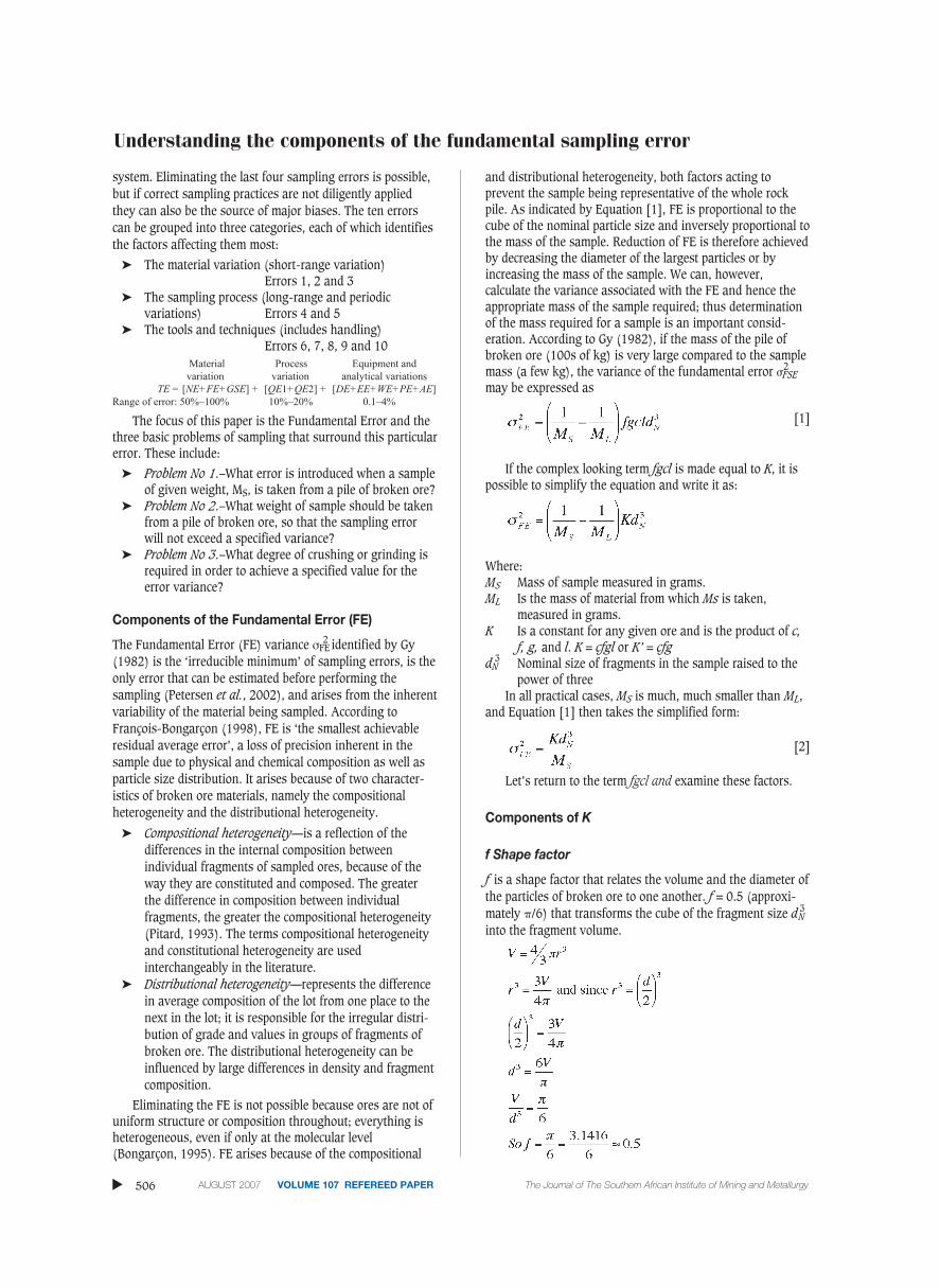
and distributional heterogeneity, both factors acting toprevent the sample being representative of the whole rockpile. As indicated by Equation [1], FE is proportional to thecube of the nominal particle size and inversely proportional tothe mass of the sample. Reduction of FE is therefore achievedby decreasing the diameter of the largest particles or byincreasing the mass of the sample. We can, however,calculate the variance associated with the FE and hence theappropriate mass of the sample required; thus determinationof the mass required for a sample is an important consid-eration. According to Gy (1982), if the mass of the pile ofbroken ore (100s of kg) is very large compared to the samplemass (a few kg), the variance of the fundamental error �2

FSEmay be expressed as

[1]

If the complex looking term fgcl is made equal to K, it ispossible to simplify the equation and write it as:

Where:MS Mass of sample measured in grams.ML Is the mass of material from which Ms is taken,

measured in grams.K Is a constant for any given ore and is the product of c,

f, g, and l. K = cfgl or K’ = cfgdN

3 Nominal size of fragments in the sample raised to thepower of three

In all practical cases, MS is much, much smaller than ML,and Equation [1] then takes the simplified form:

[2]

Let’s return to the term fgcl and examine these factors.

Components of K

f Shape factor

f is a shape factor that relates the volume and the diameter ofthe particles of broken ore to one another. f = 0.5 (approxi-mately �/6) that transforms the cube of the fragment size d 3

Ninto the fragment volume.

▲

506 AUGUST 2007 VOLUME 107 REFEREED PAPER The Journal of The Southern African Institute of Mining and Metallurgy

The product VN = fd 3N is the average volume of fragments

of nominal size dN (Bongarçon, 1998). The particle shapefactor f is an index varying between 0.1 (needles) and 1.0(cubes), but rarely exceeds the range 0.3–0.5. In practice,most values lie between 0.2 and 0.5, with the actual valuedepending on the degree to which the sample has beencrushed or pulverized. For most ores a value of f = 0.5 isused. In very fine gold ores, f = 0.2 and according to Pitard(1993), it is the shape of the metal fragment responsible forthe sample variability that is most important, so that beyondliberation it is the shape of the metal grains rather than thegangue that matters.

g Granulometric factorg is defined as the average fragment volume (V

–) divided by

the nominal fragment volume (vN) in the ratio g = V–/VNwhich is dependent on the reject percentage x used to definedN. When the average fragment volume v is multiplied by g itbecomes the average all-size fragment volume in the lot to besampled. The particle size range factor g is also known as thegrain size distribution factor (or the size range factor) andtakes values between 0 and 1; low values of g denote a largerange of particle sizes and high values denote a small range(g = 1 denotes all particles are of identical size).

When rock is crushed the product is a full distribution offragment sizes, which makes a single numerical sizeparameter that characterizes the whole fragment size distri-bution dN somewhat unrealistic. Gy examined the behaviourof the factor g as a function of the reject percentage (x) for114 combinations of crushing equipment and materials. Sixof these experimental curves are plotted in Figure 1.

The values for the reject percentage close to 5% haveminimal variability around a value of g that is reasonablyclose to 0.25 for most ores and can be estimated from theratio of the nominal top size d to the lower size limit d’(about 5% undersize) as follows:

➤ Large size range (d/d’ > 4) g = 0.25(no crushing)

➤ Medium size range (2 ≤ d/d’ ≤ 4) g = 0.50➤ Small size range (d/d’ < 2) g = 0.75➤ Uniform size (pulverized) (d/d’ = 1) g = 1.00

This approach to establishing a value for g the granu-lometry factor has been investigated in different ways by anumber of researches, but consistently achieves values ofabout 0.25. According to François-Bongarçon (1998) awayfrom the 5% reject nominal size the formula for the FE:

i. is unusable;ii. the effect of sizing on sample precision cannot be

objectively assessed, and;iii. comparing procedures across comminution devices or

types of material becomes a futile exercise.The 5% reject size (P95, for 95% passing) has with time

become the industry standard for fragment sizing. Thelognormal fragment size simulation for the usual range offragment sizes is shown in Figure 2.

c Mineralogical composition factorc is a factor for a material consisting of two components,approximately equal to the ratio of metal density (�) to thedimensionless grade of the lot (‘a’ in ‘per unit’). In itssimplest form the factor has the form:

For gold ores of very low grade where a<<1 it is possibleto use the approximation that c ≈ �m/t, where t = gold grade(g/t = g/1000000g). Because a grade of 1 ppm gold is thesame as 1g/t, which is equivalent to1 gram in 106 grams, themineralogical composition factor c for a gold grade of 1 g/tand a gold density of 19.3 g/cm3 is:

c may seem very large, but despite the units it is not adensity but, in rough terms the product of a density and alarge relative variance. Generally the mineralogicalcomposition factor is given by:

Understanding the components of the fundamental sampling errorTransaction

Paper

507The Journal of The Southern African Institute of Mining and Metallurgy VOLUME 107 REFEREED PAPER AUGUST 2007 ▲

Figure 1. Gy’s experimental grain size versus sieve size rejects (x).Source: François-Bongarçon, D. 1995. Course notes from a courseentitled ‘Sampling in the mining industry: Theory and Practice’

Figure 2. Comparison of fragment size and sieve size. Source: François-Bongarçon, D. 1995. Course notes from a course entitled ‘Sampling inthe mining industry: Theory and Practice’

Experimental material

Lognormal fragment size simulation


where:ρm = density of the metal (valuable constituent) of interest

(g/cm-3).ρg = density of the gangue (g/cm3).

a The decimal proportion or fractional concentrationof the metal of interest

a is a factor that captures the influence of the relativeproportions of the metals of interest on the mineralogicalcomposition factor, and is calculated in the following way:

➤ Zinc giving an assay of 5% and occurring as sphalerite(ZnS) would have a decimal proportion of sphalerite of:

➤ Copper giving an assay of 0.35% and occurring aschalcopyrite would have a decimal proportion ofchalcopyrite of:

This also means through this factor the sample variancedepends on the grade of the lot being sampled, and that anyuse of the formula or any sampling nomogram derived fromit, makes sense only when the grade level at which it isestablished is duly stated (François-Bongarçon, 1993 and1995, p. 477; Pitard, 1993).

Thus at 1 ppm

and the mineralogical factor is calculated as follows:

At 100 ppm c = 19.3 � 104 g/cc and at 1 000 ppm, c =19.3 x 103 g/cc. More often than not the approximation that c≈ ρm/t can be used for low concentration ores. In fact thevalue of c for gold is generally lower because most of the goldoccurs as a gold-silver amalgam that according to Pitard(2006, personal communication) has a density of around 16g/cc in which case c = 16 000 000.

In the general case the density of the crushed ore varieswith the degree of comminution and is a function of theproportions of metal and gangue. So the product cl is not avariance multiplied by a density, but is rather a density-weighted variance in which each fragment’s contribution tothe total variance is weighted by its density (François-Bongarçon, 1995; Pitard, 1993).

l Liberation factorl is a dimensionless number between 0 (no liberation) and 1(complete liberation), which varies with the size of thefragments and also depends on the nominal size of the fullyliberated metal grains. It also depends on the geostatisticalcharacteristics of the mineralization at microscopic scale, i.e.spatial correlations within the fragments. The liberation sized is the nominal size at which the fragments of the lot mustbe crushed so that the mineral grains become fully liberatedfrom the gangue and at the liberation size (as well as below)the liberation factor is equal to one. This is an ideal conceptand for practical purposes, it is the size at which approxi-mately 85 per cent of the large fragments have been liberated.The use of the value 0.5 for the exponent in this equation hasbeen the subject of some considerable discussion. Accordingto François-Bongarçon (1998, 1999), and François-Bongarçon and Gy (2002), Gy’s empirical liberation factor for

unliberated particles l = √dNdl

also written as l = (dNdl)0.5

does not

give a good result and he has suggested a more general formfor the liberation factor provides a better result as given here:

[3]

By contrast, Pitard (1993) fully supports Gy’s use of the0.5 as the exponent in Equation [3] saying that it depends onhow it is used and what the state of the broken ore is.

bIs a value related to the slope of the calibration line above theliberation size dl. The value for b can vary between 0 and 3depending on the nature of the ore and requires calibration toa particular ore type (de Castilho et al. 2005). Exponent b inEquation [3] takes values close to 1.5 in most gold ores aswell as in cases where it has not been possible to calibrate theexponent and so we can write:

Using a liberation factor b = 1.5 it is possible to producesampling nomograms that are realistic, correct and useful.

dN

Nominal size of fragments in the sample, is equivalent to themaximum particle size in the lot to be sampled. In practice, dNis taken to be the screen size that retains 5% of the lot beingsampled. For example, if a sample is sieved using a 2.5 cmaperture screen and 5% of the sample is retained on top ofthe sieve then dN = 2.50 cm. Note: In RSA sieves are referredto only by their aperture and although the old mesh notationis no longer used, it nevertheless appears on the screen nameplate.

dl liberation size and liberation factorThere is a change in the form of the relative variance of theFE when the ores become fully liberated (see Figure 3.)

Beyond liberation size further comminution does notchange the variability of the individual rock fragments(François-Bongarçon 1998). From the log-log graph of l(dl) x

▲


d3 versus fragment size (shown in Figure 3) it is known thatthe slope of the line below the liberation size (dl) is equal to3. Beyond the liberation size the slope of the line is less than3 and is given by � = 3–b and the effective range for b isactually 1 to 2. According to François-Bongarçon (2004):

where b is a factor related to the slope of the line and variesbetween 0 and 3. The underlying insight to this factor isshown in Figure 4.

Applications of Gy’s equation to the problems ofsamplingHaving derived all the components of Gy’s equation it is nowpossible to answer the questions that were posed earlier. Forthe sake of this exercise assume the following sampling

conditions for a gold bearing ore crushed to about 0.93 cm,with c = 16 000 000 for a gold-silver amalgam, f = 0.5, g =0.25 and l = 0.000035.

➤ Problem No. 1—What error is introduced when asample of given weight, MS, is taken from a pile ofbroken ore? This problem is simply answered bysubstituting the known factors into the original Gy’sequation. Assume that dN = 1.25 cm.


Paper

The Journal of The Southern African Institute of Mining and Metallurgy VOLUME 107 REFEREED PAPER AUGUST 2007 509 ▲

Figure 3. Comparison of linear fragment size with relative variance x mass. Source: François-Bongarçon, D. 1995. Course notes from a course entitled‘Sampling in the mining industry: Theory and Practice’

Figure 4. Fitting a general case to fragment sizes above and below the liberation size (0.01); Above the liberation size slope a = 3–b; below the liberationsize slope a = 3. Source: François-Bongarçon, D. 1995. Course notes from a course entitled ‘Sampling in the mining industry: Theory and Practice’

Genetic particle modelLog-log scale

Linear size of fragments


A precision of 29.58% must be compatible with the dataquality objectives of the sampling protocol for this value to beexpected.

➤ Problem No. 2—What weight of sample should betaken from a pile of broken ore, so that the samplingerror will not exceed a specified precision σFE, let ussay 15%? This requires a simple rearrangement of Gy’sequation in the form:

and the substitution of the appropriate factors to give:

A sample mass of approximately 16 kg is required toachieve a precision of 15% for this ore type.

➤ Problem No. 3—What degree of crushing or grinding isrequired in order to achieve a specified value for theerror variance σR

2? Again this requires rearrangement ofGy’s equation as follows:

Assume here that the precision is 15%, equivalent to anerror variance is 0.0225, and that the mass of material to becollected is 15 kg.

The fragment size should be 95% passing 0.9 cm toachieve a precision of 15% if a sample of 15 kg is collected.

Conclusions

Although the Fundamental Error is only one of ten samplingerrors that the practitioners needs to take cognisance of, theapproach taken by Pierre Gy provides an excellent inferentialrelationship between the mass of material to be sampled, thesize of the fragments being sampled and the relative varianceof the sampling error. It also provides solutions for three ofthe main problems associated with the Theory of Sampling.

References

PETERSEN, L., DAHL, C.K., and ESBENSEN, K.H. ACABS Research Group. Correct

Sampling—A Fundamental Prerequisite for Proper Chemical Analysis—I.

ACABS Posters. www.acabs.dk. 2002.

BRUNTON, D.W. The Theory and Practice of Ore Sampling. Transactions AIME,

vol. 836, no. 25. 1895.

DE CASTILHO, M.V., MAZZONI, P.K.M., and FRANÇOIS-BONGARÇON, D. Calibration of

parameters for estimating sampling variance. R. Holmes (ed.), Second

World Conference on Sampling and Blending, 2005. Australian Institute of

Mining and Metallurgy, Publication Series no. 4/2005. May 2005. pp. 3–8.

FRANÇOIS-BONGARÇON, D. The Practice of the Sampling of Broken Ores. CIM

Bulletin, May 1993. vol. 86, no. 970, 1993. pp. 75–81.

FRANÇOIS-BONGARÇON, D. Sampling in the Mining Industry: Theory and Practice,

Volume 1: Course notes and Transparencies. A Short Course presented by

D. François-Bongarçon in the School of Mining Engineering, University of

the Witwatersrand. 1995.

FRANÇOIS-BONGARÇON, D. The most common error in applying ‘Gy’s Formula’ in

the theory of mineral sampling. Available from D. François-Bongarçon,

President, AGORATEK International, Palo Alto, CA, USA at

www.agoratekinternational.com or [email protected]. 1998.

FRANÇOIS-BONGARÇON, D. The Modeling of the Liberation Factor and its

Calibration. Available from D. François-Bongarçon, President, AGORATEK

International, Palo Alto, CA, USA at www.agoratekinternational.com or

[email protected]. 1999.

FRANÇOIS-BONGARÇON, D. and GY, P. The most common error in applying ‘Gy’s

Formula’ in the theory of mineral sampling, and the history of the

liberation factor. South African Institute of Mining and Metallurgy

Journal, vol. 102, no. 8. 2002. pp. 475–479.

GY, P.M. The sampling of broken ores—A review of principles and practice. The

Institution of Mining and Metallurgy, London, Geological, Mining and

Metallurgical Sampling: 1973. pp. 194–205, and discussion pp. 261–263.

GY, P.M. Sampling of Particulate Materials, Theory and Practice. Developments

in Geomathematics 4. Elsevier Scientific Publishing Company. 1979. 430

pp.

GY, P.M. Sampling of Particulate Materials, Theory and Practice, Second

Revised Edition. Elsevier, Amsterdam. 1982.

GY, P.M. Sampling of Heterogeneous and Dynamic Material Systems. Theories

of heterogeneity, Sampling and Homogenising. Elsevier, Amsterdam 1992.

GY, P.M. Introduction to the Theory of Sampling. Part 1: Heterogeneity of a

Population of Uncorrelated Units. Transactions AC, 14, 1995. pp. 67–76.

GY, P.M. Sampling for Analytical Purposes: The Paris School of Physics and

Chemistry, Translated by A.G. Royle. John Wiley and Sons, Inc. New York.

1998. 153 pp.

Pitard, F.F. Pierre Gy’s sampling theory and sampling practice. Heterogeneity,

sampling correctness, and statistical process control. CRC Press, Inc.

1993. 488 pp.

PITARD, F.F. Sampling Correctness—A Comprehensive Guide. Second World

Conference on Sampling and Blending. Novotel Twin Waters Resort,

Sunshine Coast, Queensland, Australia 10-12 May 2005. pp. 55–68. ◆

Appendix 1

Below the liberation size dl

Gy’s formula can be written:

where K’ = c * f * g because below the liberation size l = 1 forall sizes.

▲


Above the liberation size dl

For the sake of this exercise assume the following samplingconditions for 10 kg of gold-bearing ore crushed to about0.93 cm. With c equal to 19 300 000, f equal to 0.5, g equalto 0.25 and l equal to 0.000035, the precision of the FE is:

In order to keep the precision below 15% either the massof the sampled material must be increased or the nominalfragment size must be reduced to say 0.93 cm.

Gy’s formula takes the form where

� = 3–b. Since we know we can substitute for l in

Gy’s equation and further write:

dl is liberation size for mineral particles, i.e. the maximumparticle diameter which ensures complete liberation of the

mineral. dl is measured in cm. Provided you have theliberation factor you can rearrange the equation

l = (dN

dl )b in its most simple form to give us dl as

follows:

In a more complex format we can derive the liberationsize as follows:

An alternative arrangement of the equation for theliberation size is as follows:

The general case for Gy’s formula can be written as

[4]

where:� = a parameter for specific deposits which can be ‘calibrated’to a particular ore type. Current research has indicated that �= 1.5 for most low grade gold ores (see1). Equation [4] canbe rearranged so that

[5]

We now have all the tools necessary to answer the threequestions stated at the beginning of the appendix.


Paper

The Journal of The Southern African Institute of Mining and Metallurgy VOLUME 107 REFEREED PAPER AUGUST 2007 511 ▲

ERRATUMERRATUM

Please note on pages 137 and 138 of the February Journal 2007, in the Comments:Mining method selection by multiple criteria decision making tool

andEQS: a computer software using fuzzy logic for equipment selection in mining engineering

By: M. Yavuz and S. PillayThe author’s name should read S. Alpay and not S. Pillay

understanding the components of the fundamental sampling error

Documents