unemployment insurance schemes and consumption: evidence...
TRANSCRIPT
Unemployment Insurance Schemes and Consumption:Evidence from Brazil
Francois Gerard (Columbia University) and Joana Naritomi (LSE)
Paris School of Economics
December 13, 2017
Francois Gerard (Columbia University) and Joana Naritomi (LSE)Unemployment Insurance Schemes and Consumption: Evidence from BrazilDecember 13, 2017
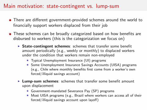
Main motivation: state-contingent vs. lump-sum
There are different government-provided schemes around the world tofinancially support workers displaced from their job
These schemes can be broadly categorized based on how benefits aredisbursed to workers (this is the categorization we focus on)
I State-contingent schemes: schemes that transfer some benefitamount periodically (e.g., weekly or monthly) to displaced workersunder the condition that workers remain non-employed
F Typical Unemployment Insurance (UI) programsF Some Unemployment Insurance Savings Accounts (UISA) programs
(e.g., Chile where monthly benefits first come from a worker’s ownforced/illiquid savings account)
I Lump-sum schemes: schemes that transfer some benefit amountupon displacement
F Government-mandated Severance Pay (SP) programsF Most UISA programs (e.g., Brazil where workers can access all of their
forced/illiquid savings account upon layoff)
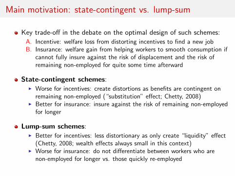
Main motivation: state-contingent vs. lump-sum
Key trade-off in the debate on the optimal design of such schemes:
A. Incentive: welfare loss from distorting incentives to find a new jobB. Insurance: welfare gain from helping workers to smooth consumption if
cannot fully insure against the risk of displacement and the risk ofremaining non-employed for quite some time afterward
State-contingent schemes:I Worse for incentives: create distortions as benefits are contingent on
remaining non-employed (“substitution” effect; Chetty, 2008)I Better for insurance: insure against the risk of remaining non-employed
for longer
Lump-sum schemes:I Better for incentives: less distortionary as only create “liquidity” effect
(Chetty, 2008; wealth effects always small in this context)I Worse for insurance: do not differentiate between workers who are
non-employed for longer vs. those quickly re-employed
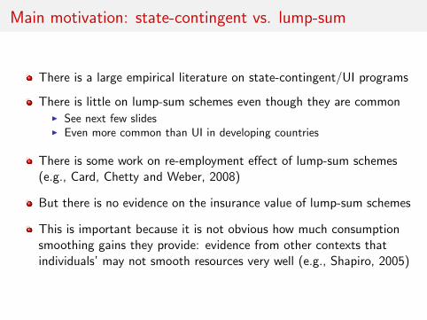
Main motivation: state-contingent vs. lump-sum
There is a large empirical literature on state-contingent/UI programs
There is little on lump-sum schemes even though they are commonI See next few slidesI Even more common than UI in developing countries
There is some work on re-employment effect of lump-sum schemes(e.g., Card, Chetty and Weber, 2008)
But there is no evidence on the insurance value of lump-sum schemes
This is important because it is not obvious how much consumptionsmoothing gains they provide: evidence from other contexts thatindividuals’ may not smooth resources very well (e.g., Shapiro, 2005)
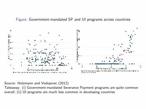
Figure: Government-mandated SP and UI programs across countries
Source: Holzmann and Vodopivec (2012)Takeaway: (i) Government-mandated Severance Payment programs are quite commonoverall; (ii) UI programs are much less common in developing countries
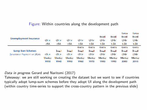
Figure: Within countries along the development path
Data in progress Gerard and Naritomi (2017)Takeaway: we are still working on creating the dataset but we want to see if countriestypically adopt lump-sum schemes before they adopt UI along the development path(within country time-series to support the cross-country pattern in the previous slide)
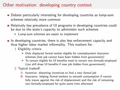
Other motivation: developing country context
Debate particularly interesting for developing countries as lump-sumschemes relatively more common
Relatively low prevalence of UI programs in developing countries couldbe due to the state’s capacity to administer such schemes
I Lump-sum schemes are easier to implement
In developing countries, there is also less enforcement capacity andthus higher labor market informality. This matters for:
1 Eligibility criteriaF Only displaced formal worker eligible for unemployment insurance
schemes (lost job cannot have been hidden from government)F To remain eligible for UI benefits need to remain non-formally-employed
(can still draw UI benefits if new job hidden from government)
2 Typical tradeoff:
A. Incentive: distorting incentives to find a new formal jobB. Insurance: helping formal workers to smooth consumption if cannot
fully insure against the risk of displacement and the risk of remainingnon-formally-employed for quite some time afterward
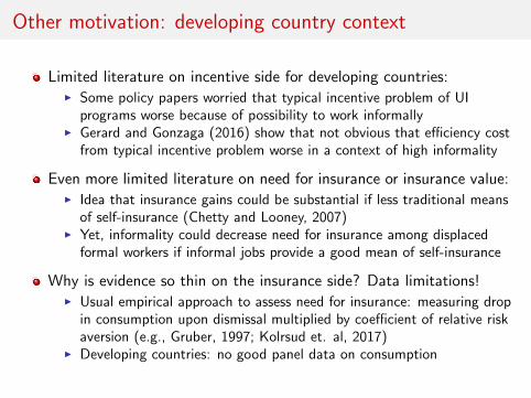
Other motivation: developing country context
Limited literature on incentive side for developing countries:I Some policy papers worried that typical incentive problem of UI
programs worse because of possibility to work informallyI Gerard and Gonzaga (2016) show that not obvious that efficiency cost
from typical incentive problem worse in a context of high informality
Even more limited literature on need for insurance or insurance value:I Idea that insurance gains could be substantial if less traditional means
of self-insurance (Chetty and Looney, 2007)I Yet, informality could decrease need for insurance among displaced
formal workers if informal jobs provide a good mean of self-insurance
Why is evidence so thin on the insurance side? Data limitations!I Usual empirical approach to assess need for insurance: measuring drop
in consumption upon dismissal multiplied by coefficient of relative riskaversion (e.g., Gruber, 1997; Kolrsud et. al, 2017)
I Developing countries: no good panel data on consumption
This paper
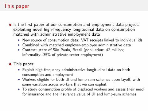
Is the first paper of our consumption and employment data project:exploiting novel high-frequency longitudinal data on consumptionmatched with administrative employment data
I New source of consumption data: VAT receipts linked to individual idsI Combined with matched employer-employee administrative dataI Context: state of Sao Paulo, Brazil (population: 42 million;
informality: 35% of private-sector employment)
This paper:I Exploit high-frequency administrative longitudinal data on both
consumption and employmentI Workers eligible for both UI and lump-sum schemes upon layoff, with
some variation across workers that we can exploitI To study consumption profile of displaced workers and assess their need
for insurance and the insurance value of UI and lump-sum schemes
Main results
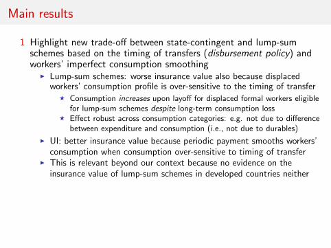
1 Highlight new trade-off between state-contingent and lump-sumschemes based on the timing of transfers (disbursement policy) andworkers’ imperfect consumption smoothing
I Lump-sum schemes: worse insurance value also because displacedworkers’ consumption profile is over-sensitive to the timing of transfer
F Consumption increases upon layoff for displaced formal workers eligiblefor lump-sum schemes despite long-term consumption loss
F Effect robust across consumption categories: e.g. not due to differencebetween expenditure and consumption (i.e., not due to durables)
I UI: better insurance value because periodic payment smooths workers’consumption when consumption over-sensitive to timing of transfer
I This is relevant beyond our context because no evidence on theinsurance value of lump-sum schemes in developed countries neither
2 Need for insurance sizable even in context of high informalityI Consumption much lower in the long-run when not eligible anymore for
any scheme (consumption drop comparable as in developed countries)I Consumption much lower immediately if not eligible for any scheme
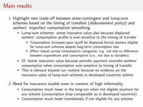
Main results
1 Highlight new trade-off between state-contingent and lump-sumschemes based on the timing of transfers (disbursement policy) andworkers’ imperfect consumption smoothing
I Lump-sum schemes: worse insurance value also because displacedworkers’ consumption profile is over-sensitive to the timing of transfer
F Consumption increases upon layoff for displaced formal workers eligiblefor lump-sum schemes despite long-term consumption loss
F Effect robust across consumption categories: e.g. not due to differencebetween expenditure and consumption (i.e., not due to durables)
I UI: better insurance value because periodic payment smooths workers’consumption when consumption over-sensitive to timing of transfer
I This is relevant beyond our context because no evidence on theinsurance value of lump-sum schemes in developed countries neither
2 Need for insurance sizable even in context of high informalityI Consumption much lower in the long-run when not eligible anymore for
any scheme (consumption drop comparable as in developed countries)I Consumption much lower immediately if not eligible for any scheme
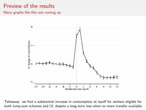
Preview of the resultsMany graphs like this one coming up
Takeaway: we find a substantial increase in consumption at layoff for workers eligible forboth lump-sum schemes and UI, despite a long-term loss when no more transfer available
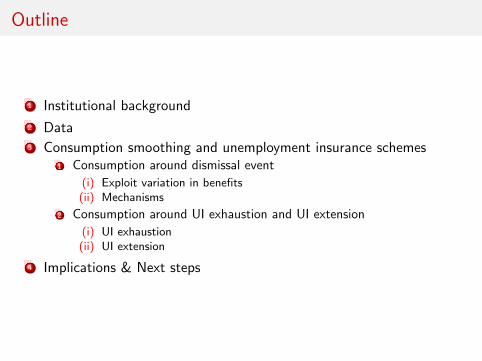
Outline
1 Institutional background
2 Data3 Consumption smoothing and unemployment insurance schemes
1 Consumption around dismissal event
(i) Exploit variation in benefits(ii) Mechanisms
2 Consumption around UI exhaustion and UI extension
(i) UI exhaustion(ii) UI extension
4 Implications & Next steps
Outline
1 Institutional background
2 Data
3 Consumption smoothing and unemployment insurance schemes
4 Implications & Next steps
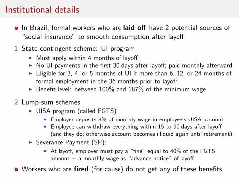
Institutional details
In Brazil, formal workers who are laid off have 2 potential sources of“social insurance” to smooth consumption after layoff
1 State-contingent scheme: UI programI Must apply within 4 months of layoffI No UI payments in the first 30 days after layoff; paid monthly afterwardI Eligible for 3, 4, or 5 months of UI if more than 6, 12, or 24 months of
formal employment in the 36 months prior to layoffI Benefit level: between 100% and 187% of the minimum wage
2 Lump-sum schemesI UISA program (called FGTS)
F Employer deposits 8% of monthly wage in employee’s UISA accountF Employee can withdraw everything within 15 to 90 days after layoff
(and they do; otherwise account becomes illiquid again until retirement)
I Severance Payment (SP):F At layoff, employer must pay a “fine” equal to 40% of the FGTS
amount + a monthly wage as “advance notice” of layoff
Workers who are fired (for cause) do not get any of these benefits
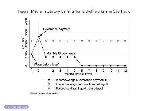
Figure: Median statutory benefits for laid-off workers in Sao Paulo
average and fired
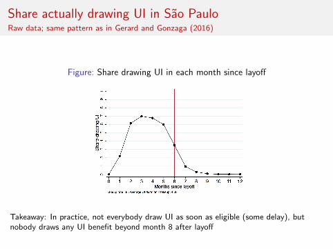
Share actually drawing UI in Sao PauloRaw data; same pattern as in Gerard and Gonzaga (2016)
Figure: Share drawing UI in each month since layoff
Takeaway: In practice, not everybody draw UI as soon as eligible (some delay), butnobody draws any UI benefit beyond month 8 after layoff
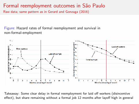
Formal reemployment outcomes in Sao PauloRaw data; same pattern as in Gerard and Gonzaga (2016)
Figure: Hazard rates of formal reemployment and survival innon-formal-employment
Takeaway: Some clear delay in formal reemployment for laid off workers (disincentiveeffect), but share remaining without a formal job 12 months after layoff high in general
Outline
1 Institutional background
2 Data
3 Consumption smoothing and unemployment insurance schemes
4 Implications & Next steps
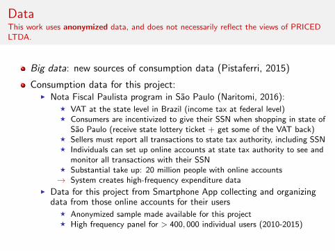
DataThis work uses anonymized data, and does not necessarily reflect the views of PRICEDLTDA.
Big data: new sources of consumption data (Pistaferri, 2015)
Consumption data for this project:I Nota Fiscal Paulista program in Sao Paulo (Naritomi, 2016):
F VAT at the state level in Brazil (income tax at federal level)F Consumers are incentivized to give their SSN when shopping in state of
Sao Paulo (receive state lottery ticket + get some of the VAT back)F Sellers must report all transactions to state tax authority, including SSNF Individuals can set up online accounts at state tax authority to see and
monitor all transactions with their SSNF Substantial take up: 20 million people with online accounts→ System creates high-frequency expenditure data
I Data for this project from Smartphone App collecting and organizingdata from those online accounts for their users
F Anonymized sample made available for this projectF High frequency panel for > 400, 000 individual users (2010-2015)
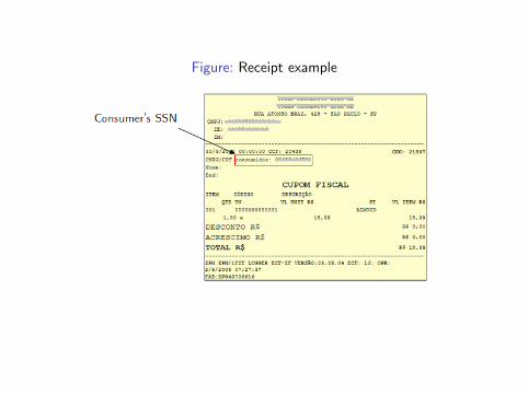
Figure: Receipt example

Data
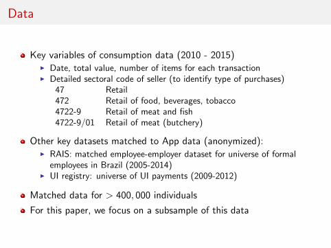
Key variables of consumption data (2010 - 2015)I Date, total value, number of items for each transactionI Detailed sectoral code of seller (to identify type of purchases)
47 Retail472 Retail of food, beverages, tobacco4722-9 Retail of meat and fish4722-9/01 Retail of meat (butchery)
Other key datasets matched to App data (anonymized):I RAIS: matched employee-employer dataset for universe of formal
employees in Brazil (2005-2014)I UI registry: universe of UI payments (2009-2012)
Matched data for > 400, 000 individuals
For this paper, we focus on a subsample of this data
Sample criteria for main analysis sample
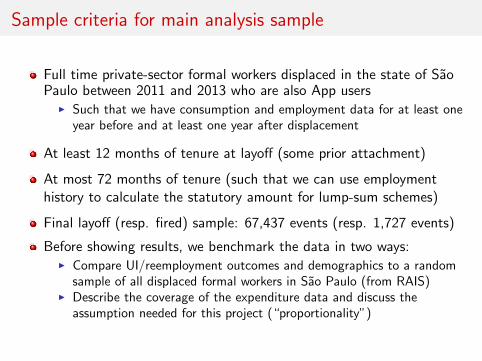
Full time private-sector formal workers displaced in the state of SaoPaulo between 2011 and 2013 who are also App users
I Such that we have consumption and employment data for at least oneyear before and at least one year after displacement
At least 12 months of tenure at layoff (some prior attachment)
At most 72 months of tenure (such that we can use employmenthistory to calculate the statutory amount for lump-sum schemes)
Final layoff (resp. fired) sample: 67,437 events (resp. 1,727 events)
Before showing results, we benchmark the data in two ways:I Compare UI/reemployment outcomes and demographics to a random
sample of all displaced formal workers in Sao Paulo (from RAIS)I Describe the coverage of the expenditure data and discuss the
assumption needed for this project (“proportionality”)
Representativeness of our main sample
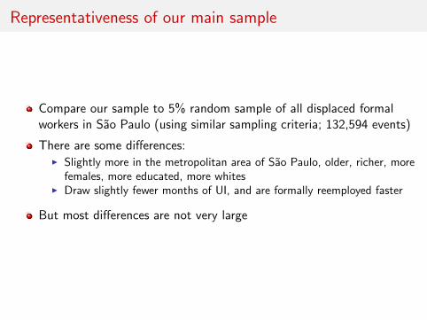
Compare our sample to 5% random sample of all displaced formalworkers in Sao Paulo (using similar sampling criteria; 132,594 events)
There are some differences:I Slightly more in the metropolitan area of Sao Paulo, older, richer, more
females, more educated, more whitesI Draw slightly fewer months of UI, and are formally reemployed faster
But most differences are not very large
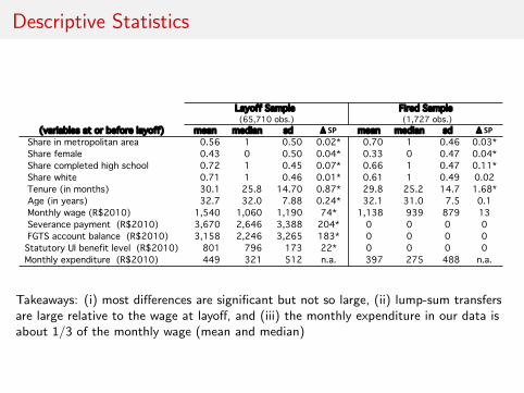
Descriptive Statistics
(variables at or before layoff) mean median sd Δ SP mean median sd Δ SP Share in metropolitan area 0.56 1 0.50 0.02* 0.70 1 0.46 0.03* Share female 0.43 0 0.50 0.04* 0.33 0 0.47 0.04* Share completed high school 0.72 1 0.45 0.07* 0.66 1 0.47 0.11* Share white 0.71 1 0.46 0.01* 0.61 1 0.49 0.02 Tenure (in months) 30.1 25.8 14.70 0.87* 29.8 25.2 14.7 1.68* Age (in years) 32.7 32.0 7.88 0.24* 32.1 31.0 7.5 0.1 Monthly wage (R$2010) 1,540 1,060 1,190 74* 1,138 939 879 13 Severance payment (R$2010) 3,670 2,646 3,388 204* 0 0 0 0 FGTS account balance (R$2010) 3,158 2,246 3,265 183* 0 0 0 0Statutory UI benefit level (R$2010) 801 796 173 22* 0 0 0 0Monthly expenditure (R$2010) 449 321 512 n.a. 397 275 488 n.a.
0.2917 0.3032 0.3487 0.2924
0 650 600 1911.81 700 620 3970.62 600 520
1950 17405850 5220
5735.3 5117.6#####
Layoff Sample Fired Sample(65,710 obs.) (1,727 obs.)
Takeaways: (i) most differences are significant but not so large, (ii) lump-sum transfersare large relative to the wage at layoff, and (iii) the monthly expenditure in our data isabout 1/3 of the monthly wage (mean and median)
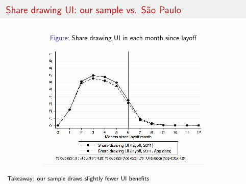
Share drawing UI: our sample vs. Sao Paulo
Figure: Share drawing UI in each month since layoff
Takeaway: our sample draws slightly fewer UI benefits
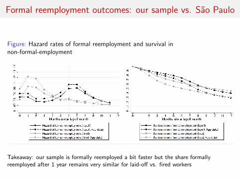
Formal reemployment outcomes: our sample vs. Sao Paulo
Figure: Hazard rates of formal reemployment and survival innon-formal-employment
Takeaway: our sample is formally reemployed a bit faster but the share formallyreemployed after 1 year remains very similar for laid-off vs. fired workers
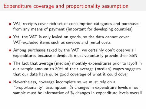
Expenditure coverage and proportionality assumption
VAT receipts cover rich set of consumption categories and purchasesfrom any means of payment (important for developing countries)
Yet, the VAT is only levied on goods, so the data cannot coverVAT-excluded items such as services and rental costs
Among purchases taxed by the VAT, we certainly don’t observe allexpenditures because individuals must voluntarily provide their SSN
The fact that average (median) monthly expenditures prior to layoff inour sample amount to 30% of their average (median) wages suggeststhat our data have quite good coverage of what it could cover
Nevertheless, coverage incomplete so we must rely on a“proportionality” assumption: % changes in expenditure levels in oursample must be informative of % changes in expenditure levels overall
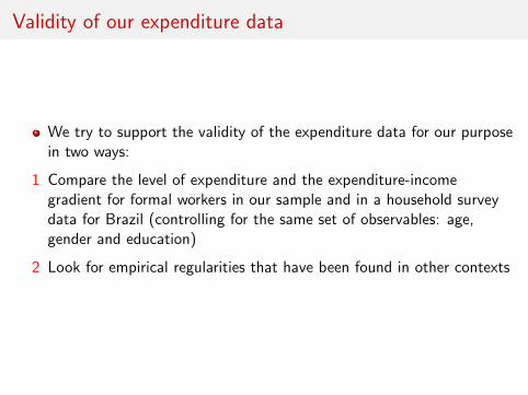
Validity of our expenditure data
We try to support the validity of the expenditure data for our purposein two ways:
1 Compare the level of expenditure and the expenditure-incomegradient for formal workers in our sample and in a household surveydata for Brazil (controlling for the same set of observables: age,gender and education)
2 Look for empirical regularities that have been found in other contexts
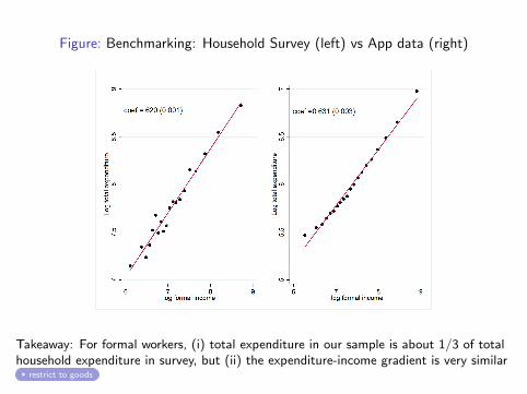
Figure: Benchmarking: Household Survey (left) vs App data (right)
Takeaway: For formal workers, (i) total expenditure in our sample is about 1/3 of totalhousehold expenditure in survey, but (ii) the expenditure-income gradient is very similar
restrict to goods
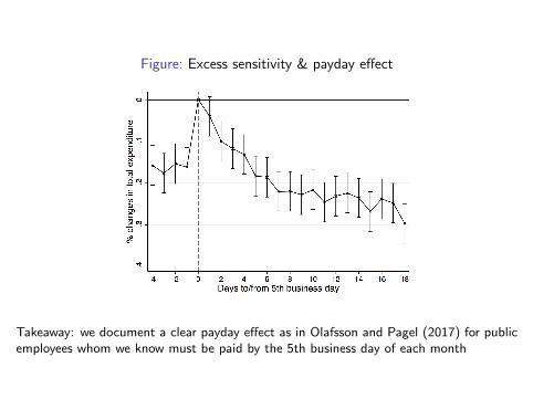
Figure: Excess sensitivity & payday effect
Takeaway: we document a clear payday effect as in Olafsson and Pagel (2017) for publicemployees whom we know must be paid by the 5th business day of each month
Outline
1 Institutional background
2 Data3 Consumption smoothing and unemployment insurance schemes
1 Consumption around dismissal event2 Consumption around UI exhaustion
4 Implications & Next steps
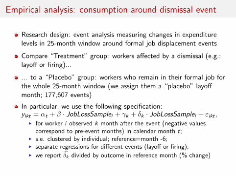
Empirical analysis: consumption around dismissal event
Research design: event analysis measuring changes in expenditurelevels in 25-month window around formal job displacement events
Compare “Treatment” group: workers affected by a dismissal (e.g.:layoff or firing)...
... to a “Placebo” group: workers who remain in their formal job forthe whole 25-month window (we assign them a “placebo” layoffmonth; 177,607 events)
In particular, we use the following specification:yikt = αt + β · JobLossSamplei + γk + δk · JobLossSamplei + εikt ,
I for worker i observed k month after the event (negative valuescorrespond to pre-event months) in calendar month t;
I s.e. clustered by individual; reference=month -6;I separate regressions for different events (layoff or firing);I we report δk divided by outcome in reference month (% change)
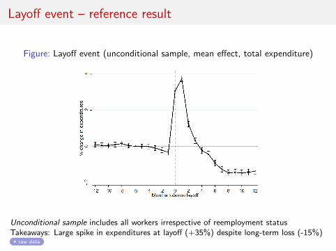
Layoff event – reference result
Figure: Layoff event (unconditional sample, mean effect, total expenditure)
Unconditional sample includes all workers irrespective of reemployment statusTakeaways: Large spike in expenditures at layoff (+35%) despite long-term loss (-15%)
raw data
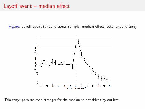
Layoff event – median effect
Figure: Layoff event (unconditional sample, median effect, total expenditure)
Takeaway: patterns even stronger for the median so not driven by outliers
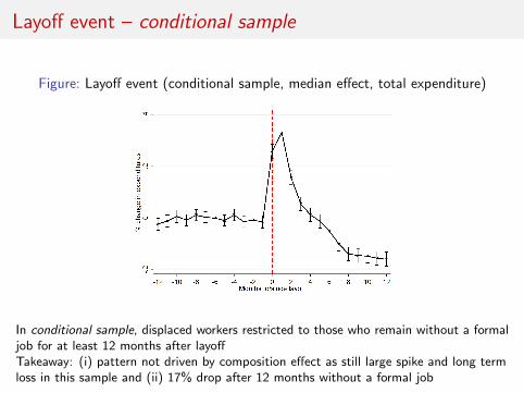
Layoff event – conditional sample
Figure: Layoff event (conditional sample, median effect, total expenditure)
In conditional sample, displaced workers restricted to those who remain without a formaljob for at least 12 months after layoffTakeaway: (i) pattern not driven by composition effect as still large spike and long termloss in this sample and (ii) 17% drop after 12 months without a formal job
Formal re-employment event
Result from similar event study around formal reemployment(placebo group used indirectly to de-trend the outcome)
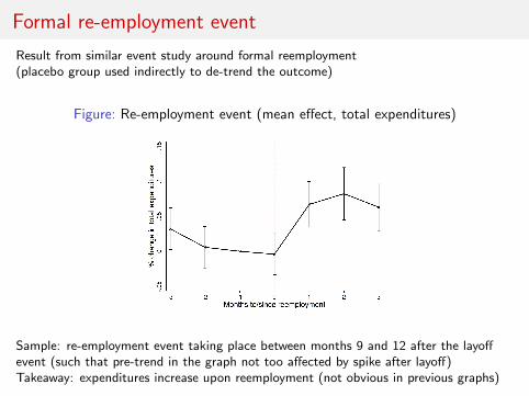
Figure: Re-employment event (mean effect, total expenditures)
Sample: re-employment event taking place between months 9 and 12 after the layoffevent (such that pre-trend in the graph not too affected by spike after layoff)Takeaway: expenditures increase upon reemployment (not obvious in previous graphs)
Dismissal event – groups with different benefits
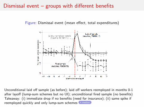
Figure: Dismissal event (mean effect, total expenditures)
Unconditional laid off sample (as before); laid off workers reemployed in months 0-1after layoff (lump-sum schemes but no UI); unconditional fired sample (no benefits)Takeaway: (i) immediate drop if no benefits (need for insurance); (ii) same spike ifreemployed quickly and only lump-sum schemes median
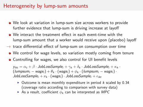
Heterogeneity by lump-sum amounts
We look at variation in lump-sum size across workers to providefurther evidence that lump-sum is driving increase at layoff
We interact the treatment effect in each event-time with thelump-sum amount that a worker would receive upon (placebo) layoff
→ trace differential effect of lump-sum on consumption over time
We control for wage levels, so variation mostly coming from tenure
Controlling for wages, we also control for UI benefit levels
yikt = αt + β · JobLossSamplei + γk + δk · JobLossSamplei + κk ·(lumpsumi − wagei ) + θk · (wagei ) + φk · (lumpsumi − wagei ) ·JobLossSamplei + νk · (wagei ) · JobLossSamplei + εikt
I Outcome is mean monthly expenditure in period k scaled by 0.34(coverage ratio according to comparison with survey data)
I As a result, coefficient φk can be interpreted as MPC
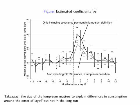
Figure: Estimated coefficients φk
Only including severance payment in lump-sum definition
Also including FGTS balance in lump-sum definition
-.05
0.0
5.1
.15
Mar
gina
l pro
pens
ity to
con
sum
e ou
t of l
ump-
sum
-12 -10 -8 -6 -4 -2 0 2 4 6 8 10 12Months to/since layoff
Takeaway: the size of the lump-sum matters to explain differences in consumptionaround the onset of layoff but not in the long run
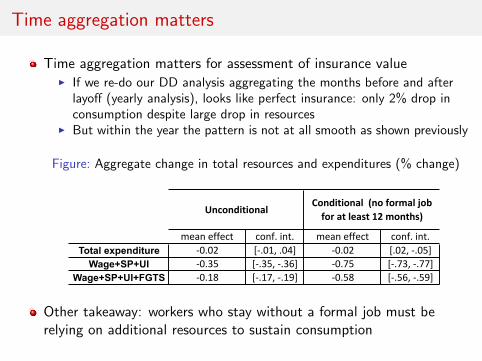
Time aggregation matters
Time aggregation matters for assessment of insurance valueI If we re-do our DD analysis aggregating the months before and after
layoff (yearly analysis), looks like perfect insurance: only 2% drop inconsumption despite large drop in resources
I But within the year the pattern is not at all smooth as shown previously
Figure: Aggregate change in total resources and expenditures (% change)
meaneffect meaneffectTotal expenditure -0.02 -0.02
Wage+SP+UI -0.35 -0.75Wage+SP+UI+FGTS -0.18 -0.58
conf.int. conf.int.
UnconditionalConditional(noformaljobforatleast12months)
[-.01,.04][-.35,-.36][-.17,-.19]
[.02,-.05][-.73,-.77][-.56,-.59]
Other takeaway: workers who stay without a formal job must berelying on additional resources to sustain consumption
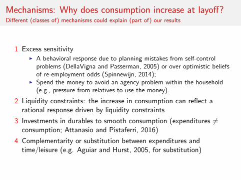
Mechanisms: Why does consumption increase at layoff?Different (classes of) mechanisms could explain (part of) our results
1 Excess sensitivityI A behavioral response due to planning mistakes from self-control
problems (DellaVigna and Passerman, 2005) or over optimistic beliefsof re-employment odds (Spinnewijn, 2014);
I Spend the money to avoid an agency problem within the household(e.g., pressure from relatives to use the money).
2 Liquidity constraints: the increase in consumption can reflect arational response driven by liquidity constraints
3 Investments in durables to smooth consumption (expenditures 6=consumption; Attanasio and Pistaferri, 2016)
4 Complementarity or substitution between expenditures andtime/leisure (e.g. Aguiar and Hurst, 2005, for substitution)
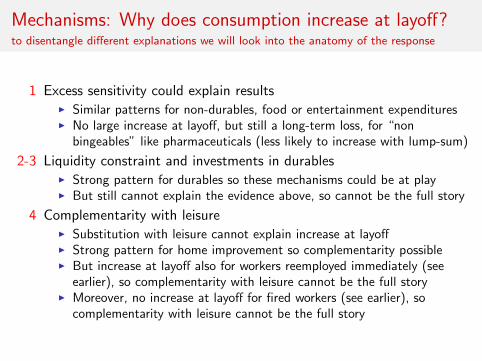
Mechanisms: Why does consumption increase at layoff?to disentangle different explanations we will look into the anatomy of the response
1 Excess sensitivity could explain resultsI Similar patterns for non-durables, food or entertainment expendituresI No large increase at layoff, but still a long-term loss, for “non
bingeables” like pharmaceuticals (less likely to increase with lump-sum)
2-3 Liquidity constraint and investments in durablesI Strong pattern for durables so these mechanisms could be at playI But still cannot explain the evidence above, so cannot be the full story
4 Complementarity with leisureI Substitution with leisure cannot explain increase at layoffI Strong pattern for home improvement so complementarity possibleI But increase at layoff also for workers reemployed immediately (see
earlier), so complementarity with leisure cannot be the full storyI Moreover, no increase at layoff for fired workers (see earlier), so
complementarity with leisure cannot be the full story
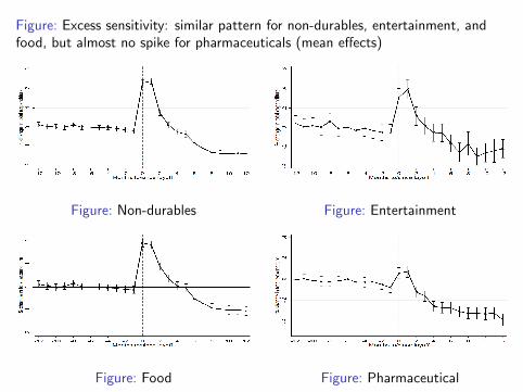
Figure: Excess sensitivity: similar pattern for non-durables, entertainment, andfood, but almost no spike for pharmaceuticals (mean effects)
Figure: Non-durables
Figure: Food
Figure: Entertainment
Figure: Pharmaceutical
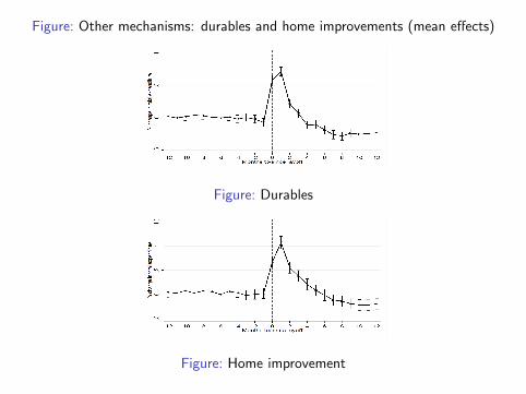
Figure: Other mechanisms: durables and home improvements (mean effects)
Figure: Durables
Figure: Home improvement
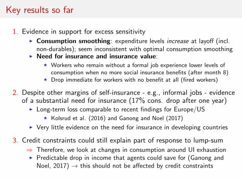
Key results so far
1. Evidence in support for excess sensitivityI Consumption smoothing: expenditure levels increase at layoff (incl.
non-durables); seem inconsistent with optimal consumption smoothingI Need for insurance and insurance value:
F Workers who remain without a formal job experience lower levels ofconsumption when no more social insurance benefits (after month 8)
F Drop immediate for workers with no benefit at all (fired workers)
2. Despite other margins of self-insurance - e.g., informal jobs - evidenceof a substantial need for insurance (17% cons. drop after one year)
I Long-term loss comparable to recent findings for Europe/USF Kolsrud et al. (2016) and Ganong and Noel (2017)
I Very little evidence on the need for insurance in developing countries
3. Credit constraints could still explain part of response to lump-sum
⇒ Therefore, we look at changes in consumption around UI exhaustionI Predictable drop in income that agents could save for (Ganong and
Noel, 2017) → this should not be affected by credit constraints
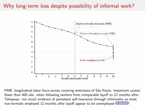
Why long-term loss despite possibility of informal work?
PME: longitudinal labor force survey covering metroarea of Sao Paulo. Important caveat:fewer than 400 obs. when following workers from comparable layoff to 12 months after.Takeaway: not much evidence of persistent self-insurance through informality as mostnon-formally employed 12 months after layoff appear to be unemployed Survival
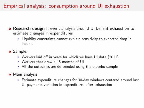
Empirical analysis: consumption around UI exhaustion
Research design I: event analysis around UI benefit exhaustion toestimate changes in expenditures
I Liquidity constraints cannot explain sensitivity to expected drop inincome
Sample:I Workers laid off in years for which we have UI data (2011)I Workers that draw all 5 months of UII All the outcomes are de-trended using the placebo sample
Main analysis:I Estimate expenditure changes for 30-day windows centered around last
UI payment: variation in expenditures after exhaustion
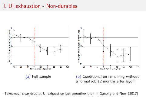
I. UI exhaustion - Non-durables
(a) Full sample (b) Conditional on remaining withouta formal job 12 months after layoff
Takeaway: clear drop at UI exhaustion but smoother than in Ganong and Noel (2017)
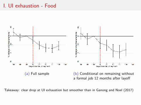
I. UI exhaustion - Food
(a) Full sample (b) Conditional on remaining withouta formal job 12 months after layoff
Takeaway: clear drop at UI exhaustion but smoother than in Ganong and Noel (2017)
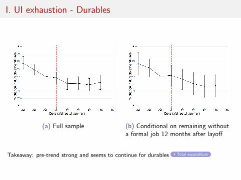
I. UI exhaustion - Durables
(a) Full sample (b) Conditional on remaining withouta formal job 12 months after layoff
Takeaway: pre-trend strong and seems to continue for durables Total expenditure
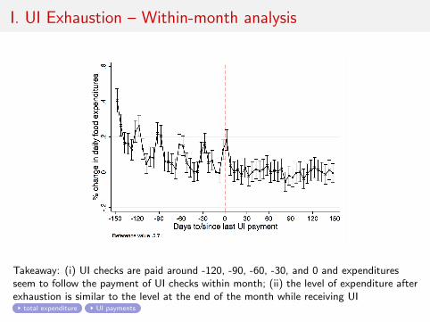
I. UI Exhaustion – Within-month analysis
Takeaway: (i) UI checks are paid around -120, -90, -60, -30, and 0 and expendituresseem to follow the payment of UI checks within month; (ii) the level of expenditure afterexhaustion is similar to the level at the end of the month while receiving UI
total expenditure UI payments
Empirical analysis: consumption around UI exhaustion
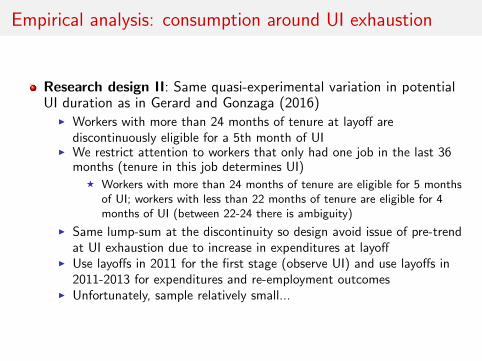
Research design II: Same quasi-experimental variation in potentialUI duration as in Gerard and Gonzaga (2016)
I Workers with more than 24 months of tenure at layoff arediscontinuously eligible for a 5th month of UI
I We restrict attention to workers that only had one job in the last 36months (tenure in this job determines UI)
F Workers with more than 24 months of tenure are eligible for 5 monthsof UI; workers with less than 22 months of tenure are eligible for 4months of UI (between 22-24 there is ambiguity)
I Same lump-sum at the discontinuity so design avoid issue of pre-trendat UI exhaustion due to increase in expenditures at layoff
I Use layoffs in 2011 for the first stage (observe UI) and use layoffs in2011-2013 for expenditures and re-employment outcomes
I Unfortunately, sample relatively small...
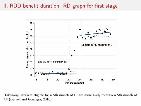
II. RDD benefit duration: RD graph for first stage
Takeaway: workers eligible for a 5th month of UI are more likely to draw a 5th month ofUI (Gerard and Gonzaga, 2016)
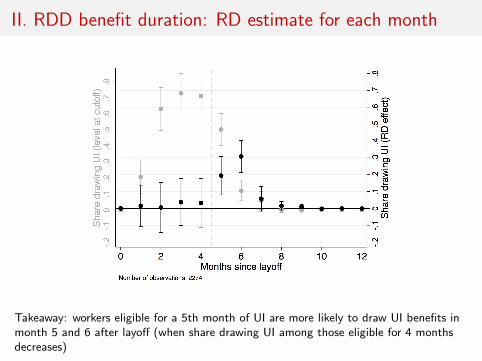
II. RDD benefit duration: RD estimate for each month
Takeaway: workers eligible for a 5th month of UI are more likely to draw UI benefits inmonth 5 and 6 after layoff (when share drawing UI among those eligible for 4 monthsdecreases)
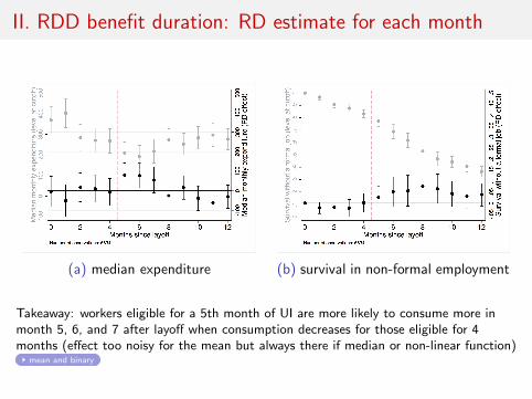
II. RDD benefit duration: RD estimate for each month
(a) median expenditure (b) survival in non-formal employment
Takeaway: workers eligible for a 5th month of UI are more likely to consume more inmonth 5, 6, and 7 after layoff when consumption decreases for those eligible for 4months (effect too noisy for the mean but always there if median or non-linear function)
mean and binary
Key results - UI exhaustion
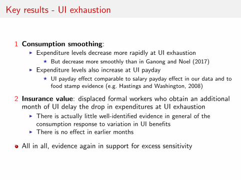
1 Consumption smoothing:I Expenditure levels decrease more rapidly at UI exhaustion
F But decrease more smoothly than in Ganong and Noel (2017)
I Expenditure levels also increase at UI paydayF UI payday effect comparable to salary payday effect in our data and to
food stamp evidence (e.g. Hastings and Washington, 2008)
2 Insurance value: displaced formal workers who obtain an additionalmonth of UI delay the drop in expenditures at UI exhaustion
I There is actually little well-identified evidence in general of theconsumption response to variation in UI benefits
I There is no effect in earlier months
All in all, evidence again in support for excess sensitivity
Outline
1 Data and Institutional background
2 Consumption smoothing and unemployment insurance schemes
3 Mechanisms
4 Implications & Next steps
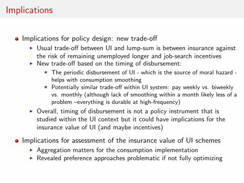
Implications
Implications for policy design: new trade-offI Usual trade-off between UI and lump-sum is between insurance against
the risk of remaining unemployed longer and job-search incentivesI New trade-off based on the timing of disbursement:
F The periodic disbursement of UI - which is the source of moral hazard -helps with consumption smoothing
F Potentially similar trade-off within UI system: pay weekly vs. biweeklyvs. monthly (although lack of smoothing within a month likely less of aproblem –everything is durable at high-frequency)
I Overall, timing of disbursement is not a policy instrument that isstudied within the UI context but it could have implications for theinsurance value of UI (and maybe incentives)
Implications for assessment of the insurance value of UI schemesI Aggregation matters for the consumption implementationI Revealed preference approaches problematic if not fully optimizing
Next steps
Estimate partial-equilibrium models of job-search and consumptionI Using reemployment data as in DellaVigna et al. (2017)I Using expenditure data as in Ganong and Noel (2017))I Benchmark model: perfectly optimizing consumer-saverI Alternate models that better fit our data: think about which moments
may distinguish different models (e.g. biased beliefs, beta-delta, etc.)
Use the estimated models to show consumption and reemploymentresponses to variations in disbursement policies
I Lump-sum vs. UI
Exploit other dimensions of the data:I Construct measures of consumption qualityI Construct individual-level measures of excess sensitivity and correlate
them across contexts (salary/UI payday, UI exhaustion, spike at layoff)
Do more forensic analysis to shed more light on role of informal sector
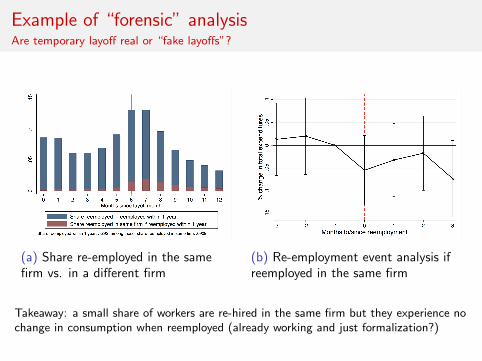
Example of “forensic” analysisAre temporary layoff real or “fake layoffs”?
(a) Share re-employed in the samefirm vs. in a different firm
(b) Re-employment event analysis ifreemployed in the same firm
Takeaway: a small share of workers are re-hired in the same firm but they experience nochange in consumption when reemployed (already working and just formalization?)

Thank you!
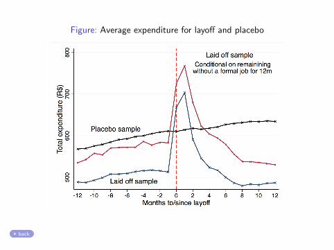
Figure: Average expenditure for layoff and placebo
back
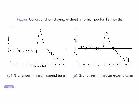
Figure: Conditional on staying without a formal job for 12 months
(a) % changes in mean expenditures (b) % changes in median expenditures
back
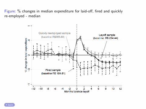
Figure: % changes in median expenditure for laid-off, fired and quicklyre-employed - median
back
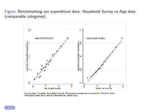
Figure: Benchmarking our expenditure data: Household Survey vs App data(comparable categories)
back
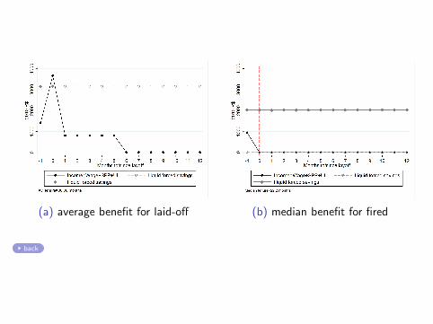
(a) average benefit for laid-off (b) median benefit for fired
back
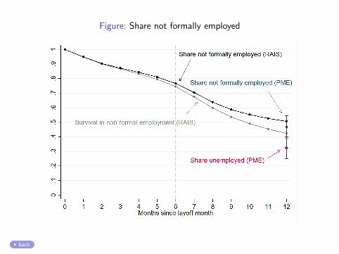
Figure: Share not formally employed
back
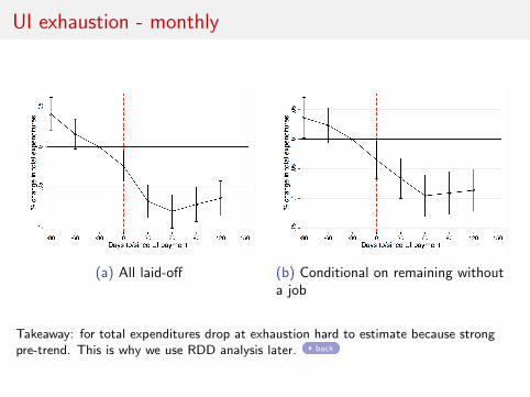
UI exhaustion - monthly
(a) All laid-off (b) Conditional on remaining withouta job
Takeaway: for total expenditures drop at exhaustion hard to estimate because strongpre-trend. This is why we use RDD analysis later. back
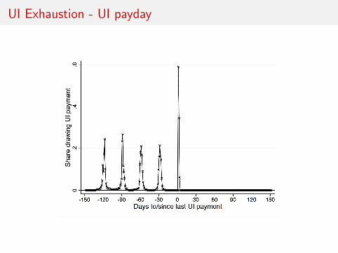
UI Exhaustion - UI payday
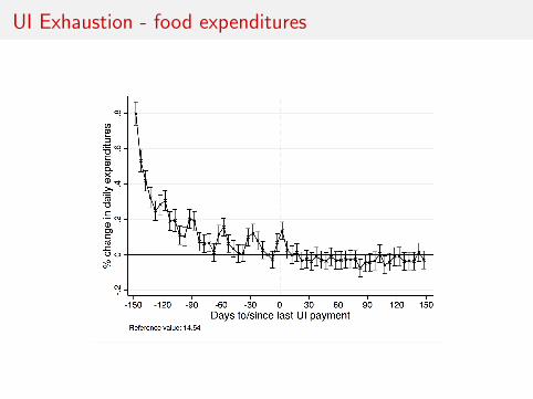
UI Exhaustion - food expenditures
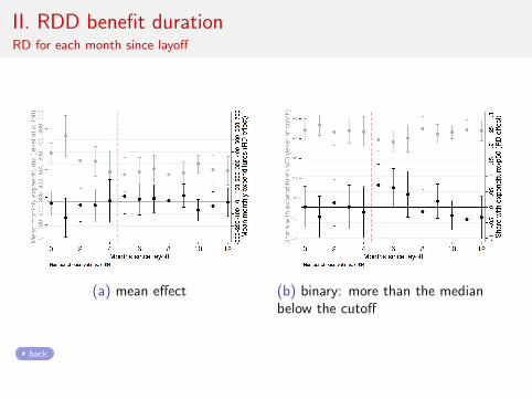
II. RDD benefit durationRD for each month since layoff
(a) mean effect (b) binary: more than the medianbelow the cutoff
back