unified segmentation - fil | ucl

www.elsevier.com/locate/ynimg

NeuroImage 26 (2005) 839–851

Unified segmentation

John AshburnerT and Karl J. Friston

Wellcome Department of Imaging Neuroscience, Functional Imaging Labolatory 12 Queen Square, London, WC1N 3BG, UK

Received 10 November 2004; revised 2 February 2005; accepted 10 February 2005

Available online 1 April 2005

A probabilistic framework is presented that enables image registration,

tissue classification, and bias correction to be combined within the

same generative model. A derivation of a log-likelihood objective

function for the unified model is provided. The model is based on a

mixture of Gaussians and is extended to incorporate a smooth intensity

variation and nonlinear registration with tissue probability maps. A

strategy for optimising the model parameters is described, along with

the requisite partial derivatives of the objective function.

D 2005 Elsevier Inc. All rights reserved.

Keywords: Image registration; Tissue classification; Bias correction;

Mixture of Gaussians; Tissue probability maps

Introduction

Segmentation of brain images usually takes one of two forms. It

can proceed by adopting a tissue classification approach, or by

registration with a template. The aim of this paper is to unify these

procedures into a single probabilistic framework.

! The first approach rests on tissue classification, whereby voxels

are assigned to a tissue class according to their intensities. In

order to make these assignments, the intensity distribution of

each tissue class needs to be characterised, often from voxels

chosen to represent each class. Automatic selection of repre-

sentative voxels can be achieved by first registering the brain

volume to some standard space, and automatically selecting

voxels that have a high probability of belonging to each class. A

related approach involves modelling the intensity distributions

by a mixture of Gaussians, but using tissue probability maps to

weigh the classification according to Bayes rule.

! The other approach involves some kind of registration, where a

template brain is warped to match the brain volume to be

segmented (Collins et al., 1995). This need not involve

matching volumes, as methods that are based on matching

1053-8119/$ - see front matter D 2005 Elsevier Inc. All rights reserved.

doi:10.1016/j.neuroimage.2005.02.018

T Corresponding author. Fax: +44 20 7813 1420.

E-mail address: [email protected] (J. Ashburner).

Available online on ScienceDirect (www.sciencedirect.com).

surfaces (MacDonald et al., 2000; Pitiot et al., 2004) would also

fall into this category. These approaches allow regions that are

pre-defined on the templates to be overlaid, allowing different

structures to be identified automatically.

A paradigm shift is evident in the field of neuroimaging

methodology, away from simple sequential processing, towards a

more integrated generative modelling approach. An example of

such an approach is the recent work by Fischl et al. (2004), with

which this paper should be compared. Both papers combine tissue

classification, bias correction, and nonlinear warping within the

same framework. Although the integrated approaches have some

disadvantages, these should be outweighed by more accurate

results. The main disadvantage is that the approaches are more

complex and therefore more difficult to implement. Implementa-

tion time is longer, more expertise is needed and the code becomes

less accessible. In addition, the algorithms are more specialised,

making it more difficult to mix and match different programs

within bpipelineQ procedures (Fissell et al., 2003; Rex et al., 2003;

Zijdenbos et al., 2002). A perceived disadvantage of these

combined models is that execution time is longer than it would

be for sequentially applied procedures. For example, optimising

two separate models with 100 parameters is likely to be faster than

optimising a combined single model with 200 parameters.

However, the reason a combined model takes longer to run is

because it actually completes the optimisation. There are usually

conditional correlations among parameters of the different models,

which sequential processing discounts. The advantage of large

models is that they are more accurate, making better use of the

information available in the data. Scanning time is relatively

expensive, but computing time is relatively cheap. Complex

models may take longer to run, but they should add value to the

raw data.

Many investigators currently use the tools within SPM1 for a

technique that has become known as boptimisedQ voxel-based

morphometry (VBM) (Good et al., 2001). VBM performs region-

wise volumetric comparisons among populations of subjects. It

requires the images to be spatially normalised, segmented into

1 Available from http://www.fil.ion.ucl.ac.uk/spm.

http:\\www.fil.ion.ucl.ac.uk

J. Ashburner, K.J. Friston / NeuroImage 26 (2005) 839–851840

different tissue classes, and smoothed, prior to performing

statistical tests. The boptimisedQ pre-processing strategy involves

spatially normalising subjects’ brain images to a standard space

by matching grey matter in these images to a grey matter

reference. The historical motivation behind this approach was to

reduce the confounding effects of non-brain (e.g., scalp) structural

variability on the registration. Tissue classification in SPM

requires the images to be registered with tissue probability maps

(Ashburner and Friston, 1997). After registration, these maps

represent the prior probability of different tissue classes being

found at each location in an image (Evans et al., 1994). Bayes

rule can then be used to combine these priors with tissue type

probabilities derived from voxel intensities to provide the

posterior probability.

This procedure is inherently circular, because the registration

requires an initial tissue classification, and the tissue classifica-

tion requires an initial registration. This circularity is resolved

here by combining both components into a single generative

model. This model also includes parameters that account for

image intensity nonuniformity, although it is now fairly standard

to include intensity nonuniformity correction in segmentation

(Wells III et al., 1996a) and registration (Friston et al., 1995;

Studholme et al., 2004) methods. Estimating the model param-

eters (for a maximum a posteriori solution) involves alternating

among classification, bias correction, and registration steps. This

approach provides better results than simple serial applications of

each component.

The objective function

In this section, we describe the model and how it is used to

define an objective function. In the next section, we will show how

this function is used to estimate the parameters of interest. The

objective function minimised by the optimum parameters is

derived from a mixture of Gaussians model. We show how this

objective function can be extended to model smooth intensity

nonuniformity. Tissue probability maps are used to assist the

classification, and we describe how the objective function

accommodates deformations of these maps, so that they best

match the image to segment. The section ends by explaining how

the estimated nonuniformity and deformations are constrained to

be spatially smooth.

Mixture of Gaussians

A distribution can be modelled by a mixture of K Gaussians

(clusters). This is a standard technique (see e.g., Bishop, 1995),

which is widely used by many tissue classification algorithms. For

univariate data, the kth Gaussian is modelled by its mean (lk),

variance (rk2) and mixing proportion (ck, where

PKk ¼ 1 ck = 1 and

ck z 0). Fitting a mixture of Gaussians (MOG) model involves

maximising the probability of observing the I elements of data y,

given the parameterisation of the Gaussians. In a simple MOG, the

probability of obtaining a datum with intensity yi given that it

belongs to the kth Gaussian (ci = k) and that the kth Gaussian is

parameterised by lk and rk2 is

P yijci ¼ k; lk ; rkð Þ ¼ 1

2pr2k

� �12

exp � yi � lkð Þ2

2r2k

! ð1Þ

The prior probability of any voxel, irrespective of its intensity,

belonging to the kth Gaussian, given the proportion of voxels that

belong to that Gaussian is simply

P ci ¼ kjckð Þ ¼ ck ð2ÞUsing Bayes rule, the joint probability of cluster k and intensity

yi is

P yi; ci ¼ kjlk ; rk ; ckð Þ

¼ P yijci ¼ k; lk ; rkð ÞP ci ¼ kjckð Þ ð3Þ

By integrating over all K clusters, we obtain the probability of

yi given the parameters

P yijm;s;gð Þ ¼XKk ¼ 1

P yi; ci ¼ kjlk ; rk ; ckð Þ ð4Þ

The probability of the entire dataset y is derived by assuming

that all elements are independent

P yjm;s;gð Þ ¼YIi ¼ 1

P yijm;s;gð Þ

¼YIi ¼ 1

XKk ¼ 1

ck

2pr2k

� �12


2r2k

! 1A

0@ ð5Þ

This probability is maximised with respect to the unknown

parameters (m, s and g), when the following cost function ðEÞ isminimised (because the two are monotonically related)

E ¼ � logP yjm;s;gð Þ

¼ �XIi ¼ 1

logXKk ¼ 1

ck

2pr2k

� �12


2r2k

! 1A

0@ ð6Þ

The assumption that voxels are independent is clearly

implausible. However, as we will see later, the priors embody a

high degree of spatial dependancy. This means that the condi-

tional probability that a voxel belongs to a tissue class shows

spatial dependencies, even though the likelihood in Eq. (5) does

not.

Intensity nonuniformity

MR images are usually corrupted by a smooth, spatially

varying artifact that modulates the intensity of the image (bias).

There are a number of sources of this artifact, which are reviewed

by Sled et al. (1998). These artifacts, although not usually a

problem for visual inspection, can impede automated processing of

the images. Early bias correction techniques involved homomor-

phic filtering, but these have generally been superceded. Most

current methods can be broadly classed as those that use

parametric representations of image intensity distributions (such

as mixtures of Gaussians) and those that use non-parametric

representations (such as histograms).

Non-parametric models usually involve image intensity histo-

grams. Some authors have proposed using a multiplicative model

of bias and optimising a function that minimises the entropy of the

histogram of the bias corrected intensities. One problem with this is

2 Available from http://www.loni.ucla.edu/ICBM/ICBM_Probabilistic.

html.

J. Ashburner, K.J. Friston / NeuroImage 26 (2005) 839–851 841

that the entropy is minimised when the bias field is uniformly zero,

resulting in a single bin containing all the counts. This was a

problem (pointed out by Arnold et al. (2001) for the bias field

correction in SPM99 (Ashburner and Friston, 2000), where there

was a tendency for the correction to reduce the mean intensity of

brain tissue in the corrected image. The constraint that the

multiplicative bias should average to unity resulted in a bowl

shaped dip in the estimated bias field.

To counter this problem, Mangin (2000) minimised the entropy

of the histograms, but included an additional term in the cost

function to minimise the squared difference between the original

and restored image mean. A related solution was devised by Likar

et al. (2001), whereby the restored image mean was constrained to

remain the same as the original. In addition to modelling a

multiplicative bias field, the latter method also modelled a smooth

additive bias. These represent partial solutions to the problem, but

are not ideal. When the width of a Gaussian (or any other

distribution) is multiplied by a factor of q, then the entropy of the

distribution is increased by log q. Therefore, when scaling data by

some value, the log of this factor needs to be considered when

developing an entropy-based cost function.

An alternative solution is to minimise the entropy of the

histogram of log-transformed intensities. In addition to being

generally better behaved, this also allows the bias fields to be

modelled as an additive effect in log-space (Sled et al., 1998). In

order to work with log-transformed data, low intensity (and

negative valued) voxels are excluded so that numerical problems

are not introduced. This exclusion motivates a more generic model

of all regional effects.

Parametric bias correction models are often an integral part of

tissue classification methods, many of which are based upon

modelling the intensities of different tissues as a mixture of

Gaussians. Other clustering methods can also be used, such as k-

means and fuzzy c-means. Additional information is often

encoded in these approaches using Markov Random Field models

to embed knowledge that neighbouring voxels are likely to

belong to the same tissue class. Most algorithms assume that the

bias is multiplicative, but there are three commonly used models

of how the bias interacts with noise. In the first parametric

model, the observed signal ( yi) is assumed to be an un-corrupted

signal (li), scaled by some bias (qi) with added Gaussian noise

(ni) that is independent of the bias (Pham and Prince, 1999;

Shattuck et al., 2001). The noise source is assumed to be from

the scanner itself

yi ¼ li=qi þ ni ð7ÞThe second model is similar to the first, except that the noise is

added before the signal is scaled. In this case, the noise is assumed

to be due to variations in tissue properties. This model is the one

used in this paper

yi ¼ li þ nið Þ=qi ð8ÞA combination of the scanner and tissue noise models has been

adopted by Fischl et al. (2004). This would probably be a better

model, especially for images corrupted by a large amount of bias.

The single noise source model was mainly chosen for its simplicity.

A third approach involves log transforming the data first,

allowing a multiplicative bias to be modelled as an additive effect

in log-space (Garza-Jinich et al., 1999; Styner, 2000; Van Leemput

et al., 1999a; Wells et al., 1996b; Zhang et al., 2001). The cost

function for these approaches is related to the entropy of the

distribution of log-transformed bias corrected data. As with the

non-parametric model based on log-transformed data, low intensity

voxels have to be excluded to avoid numerical problems. The

generative model is of a form similar to

log yi ¼ logli � logqi þ ni

yi ¼ lieni=qi ð9Þ

Sometimes these methods do not use a consistent generative model

throughout, for example when alternating between the original

intensities for the classification steps, and the log-transformed

intensities for the bias correction (Wells et al., 1996a).

In the current model, bias correction is included in the MOG by

extra parameters that account for smooth intensity variations. The

field modelling the variation at element i is denoted by q i(b),where b is a vector of unknown parameters. Intensities from the

kth cluster are assumed to be normally distributed with mean lk/

qi(b) and variance (rk/qi(b))2. Therefore, the probability of

obtaining intensity yi from the kth cluster, given its parameter-

isation, is

P yijci ¼ k; lk ; rk ;bð Þ

¼ 1

2p rk=qi bð Þð Þ2� 1

2

exp � yi � lk=qi bð Þð Þ2

2 rk=qi bð Þð Þ2

!

¼ qi bð Þ 1

2pr2k

� �12

exp � qi bð Þyi � lkð Þ2

2r2k

! ð10Þ

The tissue classification objective function is now

E ¼

�XIi¼ 1

log qi bð ÞXKk ¼ 1

ck

2pr2k

� �12

exp � qi bð Þyi � lkð Þ2

2r2k

! 1A

0@

ð11ÞThe model employed in the paper parameterises the bias as the

exponential of a linear combination of low frequency basis

functions. A small number of basis functions are used, as bias tends

to be spatially smooth. Positivity is ensured by the exponential.

Spatial priors

Rather than assuming stationary prior probabilities based upon

mixing proportions, additional information is used, based on other

subjects’ brain images. Priors are usually generated by registering a

large number of subjects together, assigning voxels to different

tissue types and averaging tissue classes over subjects. The data we

used represent a modified version of the ICBM Tissue Probabilistic

Atlas.2 They consist of tissue probability maps of grey and white

matter and of CSF (see Fig. 1). A fourth class is also used, which is

simply one minus the sum of the first three. These maps give the

prior probability of any voxel in a registered image being of any of

the tissue classes—irrespective of its intensity. The current

http:\\www.loni.ucla.edu

http:\\www.loni.ucla.edu

Fig. 1. The tissue probability maps for grey matter, white matter, CSF, and

botherQ.


implementation uses tissue probability maps for grey matter, white

matter, and CSF, although maps for additional tissue types (e.g.,

blood vessels) could also be included. The simple model of grey

matter being all of approximately the same intensity could also be

refined by using tissue probability maps for various internal grey

matter structures (Fischl et al., 2002).

The model in Eq. (11) is modified to account for these spatial

priors. Instead of using stationary mixing proportions (P(ci = kjc) =ck), the prior probabilities are allowed to vary over voxels, such

that the prior probability of voxel i being drawn from the kth

Gaussian is

P ci ¼ kjgð Þ ¼ ckbikPKj ¼ 1 cjbij

ð12Þ

where bik is the tissue probability for class k at voxel i. Note that gis no longer a vector of true mixing proportions, but for the sake of

simplicity, its elements will be referred to as such.

The number of Gaussians used to represent the intensity

distribution for each tissue class can be greater than one. In other

words, a tissue probability map may be shared by several clusters.

The assumption of a single Gaussian distribution for each class

does not hold for a number of reasons. In particular, a voxel may

not be purely of one tissue type and instead contain signal from a

number of different tissues (partial volume effects). Some partial

volume voxels could fall at the interface between different classes,

or they may fall in the middle of structures such as the thalamus,

which may be considered as being either grey or white matter.

Various image segmentation approaches use additional clusters to

model such partial volume effects. These generally assume that a

pure tissue class has a Gaussian intensity distribution, whereas

intensity distributions for partial volume voxels are broader, falling

between the intensities of the pure classes. Most of these models

assume that a mixing combination of, e.g., 50/50, is just as

probable as one of 80/20 (Laidlaw et al., 1998; Shattuck et al.,

2001; Tohka et al., 2004), whereas others allow a spatially varying

prior probability for the mixing combination, which is dependent

upon the contents of neighbouring voxels (Van Leemput et al.,

2001). Unlike these partial volume segmentation approaches, the

model adopted here simply assumes that the intensity distribution

of each class may not be Gaussian and assigns belonging

probabilities according to these non-Gaussian distributions. Select-

ing the optimal number of Gaussians per class is a model order

selection issue and will not be addressed here. Typical numbers of

Gaussians are three for grey matter, two for white matter, two for

CSF, and five for everything else.

Deformable spatial priors

The above formulation (Eq. (12)) is refined further by allowing

the tissue probability maps to be deformed according to parameters

a. This allows registration to a standard space to be included

within the same generative model.

P ci ¼ kjg;að Þ ¼ ckbik að ÞPKj ¼ 1 cjbij að Þ

ð13Þ

After including the full priors, the objective function becomes

E ¼ �XIi ¼ 1

logqi bð ÞPK

k ¼ 1 ckbik að ÞXKk ¼ 1

ckbik að Þ 2pr2k

� ��12

� exp � qi bð Þyi � lkð Þ2

2r2k

! !ð14Þ

There are many ways of parameterising how the tissue

probability maps could be deformed. Broadly speaking, these

can be described in a small- or large-deformation setting (Miller et

al., 1997). In the small deformation setting, a spatial mapping is

usually parameterised by adding a linear combination of basis

functions to the identity transform, or to some initial affine

transform. These bases can be global, such as polynomial (Woods

et al., 1998a,b) or cosine transform bases (Ashburner and Friston,

1999). They can be intermediate, such as the approaches

parameterised by B-splines (Kybic and Unser, 2003; Rueckert et

al., 1999), or they can be very local. Some very high-dimensional

finite difference approaches fit into this category. The registration

procedure involves estimating the bbestQ linear combination by

optimising an objective function, normally consisting of the sum

of log-likelihood and prior terms. The prior term provides stability,

often in the form of linear regularisation. Linear regularisation

methods include simultaneously minimising membrane (Amit et

al., 1991; Gee et al., 1997), linear elastic (Davatzikos, 1996;

Miller et al., 1993), or bending energy (Bookstein, 1997). An

alternative regularisation approach is to smooth the displacements

at each iteration of the registration (Collins et al., 1994). This too

is a form of linear regularisation (Bro-Nielsen and Gramkow,

1996). Without incorporating additional constraints (positive

Jacobian determinants), the small deformation approaches using

linear regularisation do not necessarily enforce a one-to-one

mapping (see e.g., Christensen et al., 1995) in the spatial

transformation, although prior terms that incorporate this con-

straint have been devised (Ashburner et al., 1999; Edwards et al.,

1997).


The large deformation setting allows more shape variability to

be modelled, while still retaining a smooth continuous one-to-one

mapping (diffeomorphism). Rather than parameterising in terms

of the deformations themselves, these approaches involve a

parameterisation based on velocities. Spatial transformations are

then computed by integrating the velocities over time. Most

current implementations of large deformation registration are

derived from the greedy viscous fluid registration of Christensen

et al. (1996) or the related technique of Thirion (1995). These

approaches have the disadvantage that they can produce

unpredictable solutions if allowed to iterate indefinitely. The

regularisation is based on penalising deviations between the

current and previous estimates, rather than deviations away from

the identity transform (it is bplasticQ, rather than belasticQ).Penalising the warps is therefore more akin to modelling

viscosity, rather than elasticity. A number of improvements have

since been made in the field of large deformation image

registration, placing it within a much more elegant theoretical

framework (Miller, 2004; Miller and Younes, 2001).

Our current implementation uses a low-dimensional approach,

which parameterises the deformations by a linear combination of

about a thousand cosine transform bases (Ashburner and Friston,

1999). This is not an especially precise way of encoding

deformations, but it can model the variability of overall brain

shape. Evaluations have shown that this simple model can

achieve a registration accuracy comparable to other fully

automated methods with many more parameters (Hellier et al.,

2001, 2002).

Regularisation

One important issue relates to the distinction between intensity

variations that arise because of bias artifact due to the physics of

MR scanning and those that arise due to different tissue

properties. The objective is to model the latter by different tissue

classes, while modelling the former with a bias field. We know a

priori that intensity variations due to MR physics tend to be

spatially smooth, whereas those due to different tissue types tend

to contain more high frequency information. A more accurate

estimate of a bias field can be obtained by including prior

knowledge about the distribution of the fields likely to be

encountered by the correction algorithm. For example, if it is

known that there is little or no intensity nonuniformity, then it

would be wise to penalise large values for the intensity

nonuniformity parameters. This regularisation can be placed

within a Bayesian context, whereby the penalty incurred is the

negative logarithm of a prior probability for any particular pattern

of nonuniformity. Similarly, it is possible for intensity variations

to be modelled by incorrect registration. If we had some

knowledge about a prior probability distribution for brain shape,

then this information could be used to regularise the deformations.

It is not possible to determine a complete specification of such a

probability distribution empirically. Instead, the current approach

(as with most other nonlinear registration procedures) uses an

educated guess for the form and amount of variability likely to be

encountered. Without such regularisation, the pernicious inter-

actions (Evans, 1995) among the parameter estimates could be

more of a problem. With the regularisation terms included, fitting

the model involves maximising

P y;b;ajg; l;s2� �

¼ P yjb;a;g; l;s2� �

P bð ÞP að Þ ð15Þ

This is equivalent to minimising

F ¼ � logP y;b;ajg; l;s2� �

¼ E � logP bð Þ � logP að Þð16Þ

In the current implementation, the probability densities of the

spatial parameters are assumed to be zero-mean multivariate

Gaussians (P(a) = N(0, Ca) and P(b) = N(0,Cb)). For the

nonlinear registration parameters, the covariance matrix is defined

such that aTCa�1a gives the bending energy of the deformations

(see Ashburner et al., 1999 for details). The prior covariance

matrix for the bias is based on the assumption that a typical bias

field could be generated by smoothing zero mean random

Gaussian noise by a broad Gaussian smoothing kernel (about

70 mm FWHM), and then exponentiating (that is, Cb is a

Gaussian Toeplitz matrix).

Optimisation

This section describes how the objective function from Eqs.

(14) and (16) is minimised (i.e., how the model is fitted). There is

no closed form solution for finding the parameters, and optimal

values for different parameters are dependent upon the values of

others. An Iterated Conditional Modes (ICM) approach is used. It

begins by assigning starting estimates for the parameters and then

iterating until a locally optimal solution is found. Each iteration

involves alternating between estimating different groups of

parameters, while holding the others fixed at their current bbestQsolution (i.e., conditional mode). The mixture parameters are

updated using an Expectation Maximisation (EM) algorithm,

while holding the bias and deformations fixed at their conditional

modes. The bias is estimated while holding the mixture

parameters and deformation constant. Because intensity nonun-

iformity is very smooth, it can be described by a small number of

parameters, making the Levenberg–Marquardt (LM) scheme ideal

for this optimisation. The deformations of the tissue probability

maps are re-estimated while fixing the mixture parameters and

bias field. A low-dimensional parameterisation is used for the

deformations, so the LM strategy is also applicable here.

The procedure is a local optimisation, so it needs reasonable

initial starting estimates. Starting estimates for the cluster para-

meters are randomly assigned. Coefficients for the bias and

nonlinear deformations are initially set to zero, but an affine

registration using the objective function of D’Agostino et al. (2004)

is used to approximately align with the tissue probability maps.

The model is only specified for brain, as there are no tissue

probability maps for non-brain tissue (scalp etc.). Because of this,

there is a tendency for the approach to stretch the probability maps

so that the background class contains only air, but no scalp. A

workaround involves excluding extra-cranial voxels from the

fitting procedure. This is done by fitting a mixture of two

Gaussians to the image intensity histogram. In most cases, one

Gaussian fits air, and the other fits everything else. A suitable

threshold is then determined, based on a 50% probability. Fitting

only the intra-cranial voxels also saves time.

Mixture parameters (m, s2 and g )

It is sufficient to minimise E with respect to the mixture

parameters because they do not affect the prior or regularisation


terms in calF (see Eq. (16)). For simplicity, we will summarise the

parameters of interest by q = {m, s, g , a, b}. These are optimised

by EM (see e.g., Bishop, 1995; Dempster et al., 1977; Neal and

Hinton, 1998), which can be considered as using some distribution,

qik, to minimise the following upper bound on E

E V EEM ¼ �XIi ¼ 1

logP yijqð Þ

þXIi ¼ 1

XKk ¼ 1

qik logqik

P ci ¼ kjyi; qð Þ

��ð17Þ

EM is an iterative approach and involves alternating between

an E-step (which minimises EEM with respect to qik) and an M-

step (which minimises EEM with respect to q). The second term

of Eq. (17) is a Kullback–Leibler distance, which is at a minimum

of zero when qik = P(ci = kjyi, q), and Eq. (17) becomes an

equality (E ¼ EEM). Because qik does not enter into the first term,

the E-step of iteration n consists of setting

qnð Þik ¼ Pðci ¼ kjyi; q nð ÞÞ ¼

P yi; ci ¼ kjq nð Þ� P yijq nð Þ� ¼ pikPK

j ¼ 1 pijð18Þ

where

pik ¼ckbik að ÞPKj ¼ 1 cjbij að Þ

2pr2k

� ��12exp � qi bð Þyi � lkð Þ2

2r2k

! ð19Þ

qik represents the posterior or conditional probabilities of ci = k

that we are interested in. The M-step uses the recently updated

values of qik(n) in order to minimise E with respect to q. Eq. (17)

can be reformulated3 as

E ¼ EEM ¼ �XIi ¼ 1

XKk ¼ 1

qik logP yi; ci ¼ kjqð Þ

þXIi ¼ 1

XKk ¼ 1

qik log qik ð20Þ

Because the second term is independent of q, the M-step involves

assigning new values to the parameters, such that the derivatives of

the following are zero

�XIi ¼ 1

XKk ¼ 1

qik logP yi; ci ¼ kjqð Þ

¼XIi ¼ 1

XKk ¼ 1

qik logXKj ¼ 1

cjbij að Þ! � log ck

!

þXIi ¼ 1

XKk ¼ 1

qik1

2log r2

k

� �þ 1

2r2qi bð Þyi � lkð Þ2

��

þXIi ¼ 1

XKk ¼ 1

qik1

2log 2pð Þ � log qi bð Þbik að Þð Þ

��ð21Þ

Differentiating Eq. (21) with respect to lk gives

BFBlk

¼ BEBlk

¼XIi ¼ 1

qnð Þik

r2k

lk � qi bð Þyið Þ ð22Þ

3 Through Bayes rule, and becausePK

k ¼ 1 qik ¼ 1, we obtain log

P yijqð Þ ¼ logP yi;ci ¼ kjqð ÞP ci ¼ kjyi;qð Þ

�¼PK

k ¼ 1qik log

P yi;ci ¼ kjqð ÞP ci ¼ kjyiqð Þ

�.

This gives the update formula for lk by solving for BeBlk

¼ 0

l n þ 1ð Þk ¼

PIi ¼ 1 q

nð Þik qi bð ÞyiPI

i ¼ 1 qnð Þik

ð23Þ

Similarly, differentiating Eq. (21) with respect to rk2

BFBr2

k

¼ BEBr2

k

¼PI

i ¼ 1 qnð Þik

2r2k

�PI

i ¼ 1 qnð Þik lk � qi bð Þyið Þ2

2 r2k

� �2 ð24Þ

This gives the update formula for rk2

r2k

� � n þ 1ð Þ ¼PI

i ¼ 1 qnð Þik l n þ 1ð Þ

k � qi bð Þyi� 2PI

i ¼ 1 qnð Þik

ð25Þ

Differentiating Eq. (21) with respect to ck

BFBck

¼ BEBck

¼XIi ¼ 1

bik að ÞPKj ¼ 1 cjbij að Þ

�PI

i ¼ 1 qnð Þik

ckð26Þ

Deriving an exact update scheme for gk is difficult, but the

following ensures convergence4

c n þ 1ð Þk ¼

PIi ¼ 1 q

nð ÞikPI

i ¼ 1bik að ÞPK

j ¼ 1c nð Þjbij að Þ

ð27Þ

Bias (b)

The next step is to update the estimate of the bias field. This

involves holding the other parameters fixed and improving the

estimate of b using an LM optimisation approach (see Press et al.,

1992 for more information). Each iteration requires the first and

second derivatives of the objective function, with respect to the

parameters. In the following scheme, I is an identity matrix and k is a

scaling factor. The choice of k is a trade-off between speed of

convergence and stability. A value of zero for k gives the Newton–

Raphson or Gauss–Newton optimisation scheme, which may be

unstable. Increasing k will slow down the convergence but increase

the stability of the algorithm. The value of k is usually decreased

slightly after iterations thatdecrease (improve) thecost function. If the

cost function increases after an iteration, then the previous solution is

retained, and k is increased in order to provide more stability.

b n þ 1ð Þ ¼ b nð Þ � B2F

Bb2

��b nð Þ

þ kI

1A

0@

�1

BF

Bb

��b nð Þ

ð28Þ

The prior probability of the parameters is modelled by a

multivariate Gaussian density, with mean b0 and covariance Cb.

� logP bð Þ ¼ 1

2b� b0ð ÞC�1

b b� b0ð Þ þ const ð29Þ

The first and second derivatives of F (see Eq. (16)) with respect to

the parameters are therefore

BFBb

¼ BEBb

þ C�1b b� b0ð Þ and B

2FBb2

¼ B2E

Bb2þ C�1

b ð30Þ

4 The update scheme was checked empirically and found to always

reduce E. It does not fully minimise it though, which means that this part of

the algorithm is really a Generalised EM.


The first and second partial derivatives of E are

BEBbm

¼ �XIi ¼ 1

BqibBbm

qi bð Þ�1 þ yiXKk ¼ 1

qik lk � q bð Þyið Þr2k

!

ð31Þ

B2E

Bbmbn

¼XIi ¼ 1

Bqi bð ÞBbm

Bqi bð ÞBbn

qi bð Þ�2 þ y2i

XKk ¼ 1

qik

r2k

!

�XIi ¼ 1

B2qi bð Þ

BbmBbn

qi bð Þ�1 þ yiXKk ¼ 1

qik lk � qi bð Þyið Þr2k

!

ð32ÞThe bias field is parameterised by the exponential of a linear

combination of smooth basis functions

qi bð Þ ¼ expXM

m ¼ 1

bmwim

! ;Bqi bð ÞBbm

¼ wimqi bð Þ;

andB2qiðbÞ

BbmBbn

¼ wimwinqi bð Þ ð33Þ

Therefore, the derivatives used by the optimisation are

BEBbm

¼ �XIi ¼ 1

wim 1þ qi bð ÞyiXKk ¼ 1


!

B2E

Bbmbn

¼XIi ¼ 1

wimwin qi bð Þyið Þ2XKk ¼ 1

qik

r2k

� qi bð Þyi

�XKk ¼ 1


! ð34Þ

Deformations (a)

The same LM strategy (Eq. (28)) is used as for updating the

bias. Schemes such as LM or Gauss–Newton are usually used only

for registering images with a mean squared difference objective

function, although some rare exceptions exist where LM has been

applied to information-theoretic image registration (Thevenaz and

Unser, 2000). The strategy requires the first and second derivatives

of the cost function, with respect to the parameters that define the

deformation. In order to simplify deriving the derivatives, the

likelihood component of the objective function is re-expressed as

E ¼XIi ¼ 1

logXKk ¼ 1

fik lik

! �XIi ¼ 1

logqi bð Þ ð35Þ

where

fik ¼bik að ÞPK

j ¼ 1 cjbij að Þð36Þ

and

lik ¼ ck 2pr2k

� ��12exp � qi bð Þyi � lkð Þ2

2r2k

! ð37Þ

The first derivatives of E with respect to a are

BEBam

¼ �XIi ¼ 1

PKk ¼ 1

BfikBam

likPKk ¼ 1 fik lik

ð38Þ

The second derivatives are

B2E

BamBan¼XIi ¼ 1

PKk ¼ 1

BfikBam

lik

� PKk ¼ 1

BfikBan

lik

�PK

k ¼ 1 fik lik

� 2

�XIi ¼ 1

PKk ¼ 1

B2 fik

BamBanlikPK

k ¼ 1 fik likð39Þ

The following is needed in order to compute derivatives of Ewith respect to a.

Bfik

Bam¼

Bbik að ÞBamPK

j ¼ 1 cjbij að Þ�

bik að ÞPK

j ¼ 1 cjBbij að ÞBamPK

j ¼ 1 cjbij að Þ � 2

ð40Þ

The second term in Eq. (39) is ignored in the optimisation

(Gauss–Newton approach), but it could be used (Newton–Raphson

approach). These gradients and curvatures enter the update scheme

as in Eq. (28).

The chain rule is used to compute derivatives of fik based on the

rate of change of the deformation fields with respect to changes of

the parameters, and the tissue probability map gradients sampled at

the appropriate points. Trilinear interpolation could be used as the

tissue probability maps contain values between zero and one. Care

is needed when attempting to sample the images with higher

degree B-spline interpolation (Thevenaz et al., 2000), as negative

values should not occur. B-spline interpolation (and other

generalised interpolation methods) requires coefficients to be

estimated first. This essentially involves deconvolving the B-spline

bases from the image (Unser et al., 1993a,b). Sampling an

interpolated value in the image is then done by re-convolving the

coefficients with the B-spline. Without any non-negativity con-

straints on the coefficients, there is a possibility of negative values

occurring in the interpolated probability map.

One possible solution is to use a maximum likelihood

deconvolution strategy to estimate some suitable coefficients. This

is analogous to the iterative method for maximum likelihood

reconstruction of PET images (Shepp and Vardi, 1982) or to the

way that mixing proportions are estimated within a mixture of

Gaussians model. A second solution is to add a small background

value to the probability maps and take a logarithm. Standard

interpolation methods could be applied to the log-transformed data

before exponentiating again. Neither of these approaches is really

optimal. In practice, 3rd degree B-spline interpolation is used, but

without first deconvolving. This introduces a small, but acceptable,

amount of additional smoothness to the tissue probability maps.

Evaluation

Generally, the results of an evaluation are specific only to the

data used to evaluate the model. MR images vary a great deal with

different subjects, field strengths, scanners, sequencies etc, so a

model that is good for one set of data may not be appropriate for

another. For example, consider intra-subject brain registration,

under the assumption that the brain behaves like a rigid body. If the

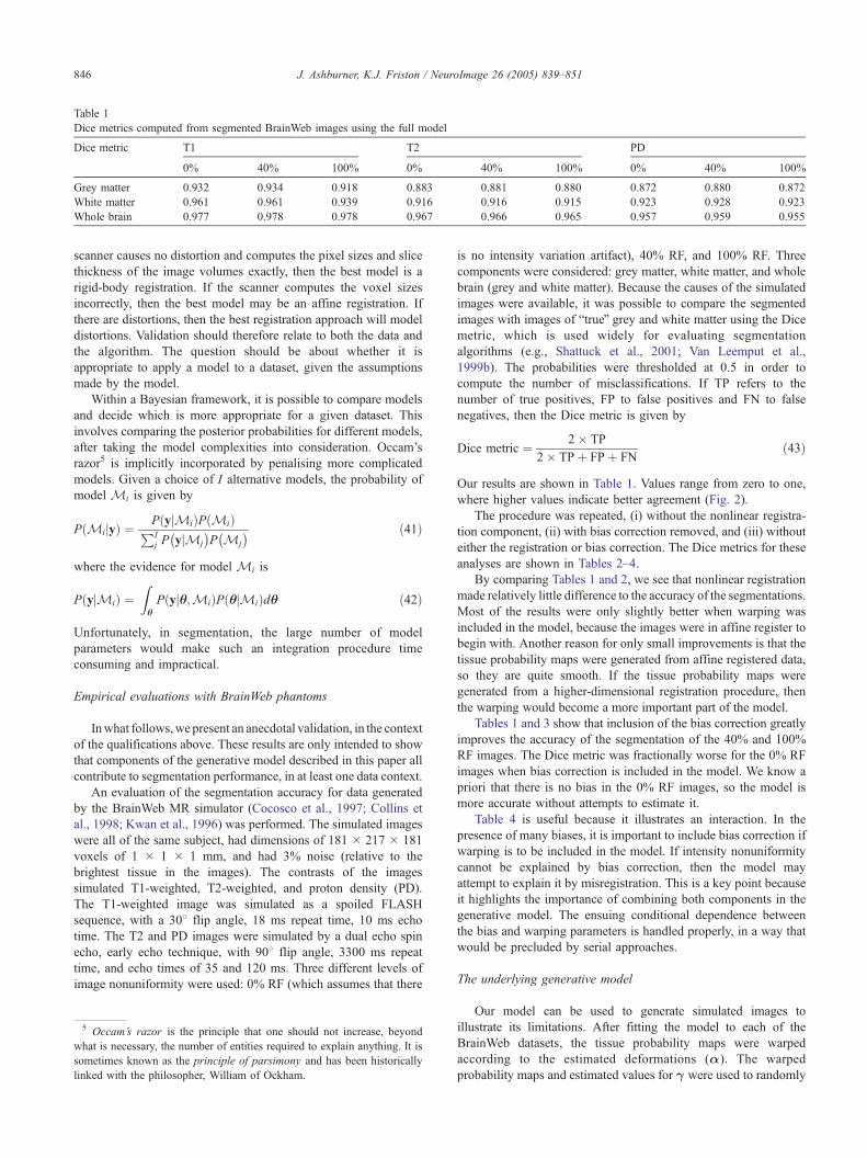
Table 1

Dice metrics computed from segmented BrainWeb images using the full model

Dice metric T1 T2 PD

0% 40% 100% 0% 40% 100% 0% 40% 100%

Grey matter 0.932 0.934 0.918 0.883 0.881 0.880 0.872 0.880 0.872

White matter 0.961 0.961 0.939 0.916 0.916 0.915 0.923 0.928 0.923

Whole brain 0.977 0.978 0.978 0.967 0.966 0.965 0.957 0.959 0.955


scanner causes no distortion and computes the pixel sizes and slice

thickness of the image volumes exactly, then the best model is a

rigid-body registration. If the scanner computes the voxel sizes

incorrectly, then the best model may be an affine registration. If

there are distortions, then the best registration approach will model

distortions. Validation should therefore relate to both the data and

the algorithm. The question should be about whether it is

appropriate to apply a model to a dataset, given the assumptions

made by the model.

Within a Bayesian framework, it is possible to compare models

and decide which is more appropriate for a given dataset. This

involves comparing the posterior probabilities for different models,

after taking the model complexities into consideration. Occam’s

razor5 is implicitly incorporated by penalising more complicated

models. Given a choice of I alternative models, the probability of

model Mi is given by

P Mijyð Þ ¼ P yjMið ÞP Mið ÞPIj P yjMj

� �P Mj

� � ð41Þ

where the evidence for model Mi is

P yjMið Þ ¼ZqP yjq;Mið ÞP qjMið Þdq ð42Þ

Unfortunately, in segmentation, the large number of model

parameters would make such an integration procedure time

consuming and impractical.

Empirical evaluations with BrainWeb phantoms

Inwhat follows,we present an anecdotal validation, in the context

of the qualifications above. These results are only intended to show

that components of the generative model described in this paper all

contribute to segmentation performance, in at least one data context.

An evaluation of the segmentation accuracy for data generated

by the BrainWeb MR simulator (Cocosco et al., 1997; Collins et

al., 1998; Kwan et al., 1996) was performed. The simulated images

were all of the same subject, had dimensions of 181 � 217 � 181

voxels of 1 � 1 � 1 mm, and had 3% noise (relative to the

brightest tissue in the images). The contrasts of the images

simulated T1-weighted, T2-weighted, and proton density (PD).

The T1-weighted image was simulated as a spoiled FLASH

sequence, with a 308 flip angle, 18 ms repeat time, 10 ms echo

time. The T2 and PD images were simulated by a dual echo spin

echo, early echo technique, with 908 flip angle, 3300 ms repeat

time, and echo times of 35 and 120 ms. Three different levels of

image nonuniformity were used: 0% RF (which assumes that there

5 Occam’s razor is the principle that one should not increase, beyond

what is necessary, the number of entities required to explain anything. It is

sometimes known as the principle of parsimony and has been historically

linked with the philosopher, William of Ockham.

is no intensity variation artifact), 40% RF, and 100% RF. Three

components were considered: grey matter, white matter, and whole

brain (grey and white matter). Because the causes of the simulated

images were available, it was possible to compare the segmented

images with images of btrueQ grey and white matter using the Dice

metric, which is used widely for evaluating segmentation

algorithms (e.g., Shattuck et al., 2001; Van Leemput et al.,

1999b). The probabilities were thresholded at 0.5 in order to

compute the number of misclassifications. If TP refers to the

number of true positives, FP to false positives and FN to false

negatives, then the Dice metric is given by

Dice metric ¼ 2� TP

2� TPþ FPþ FNð43Þ

Our results are shown in Table 1. Values range from zero to one,

where higher values indicate better agreement (Fig. 2).

The procedure was repeated, (i) without the nonlinear registra-

tion component, (ii) with bias correction removed, and (iii) without

either the registration or bias correction. The Dice metrics for these

analyses are shown in Tables 2–4.

By comparing Tables 1 and 2, we see that nonlinear registration

made relatively little difference to the accuracy of the segmentations.

Most of the results were only slightly better when warping was

included in the model, because the images were in affine register to

begin with. Another reason for only small improvements is that the

tissue probability maps were generated from affine registered data,

so they are quite smooth. If the tissue probability maps were

generated from a higher-dimensional registration procedure, then

the warping would become a more important part of the model.

Tables 1 and 3 show that inclusion of the bias correction greatly

improves the accuracy of the segmentation of the 40% and 100%

RF images. The Dice metric was fractionally worse for the 0% RF

images when bias correction is included in the model. We know a

priori that there is no bias in the 0% RF images, so the model is

more accurate without attempts to estimate it.

Table 4 is useful because it illustrates an interaction. In the

presence of many biases, it is important to include bias correction if

warping is to be included in the model. If intensity nonuniformity

cannot be explained by bias correction, then the model may

attempt to explain it by misregistration. This is a key point because

it highlights the importance of combining both components in the

generative model. The ensuing conditional dependence between

the bias and warping parameters is handled properly, in a way that

would be precluded by serial approaches.

The underlying generative model

Our model can be used to generate simulated images to

illustrate its limitations. After fitting the model to each of the

BrainWeb datasets, the tissue probability maps were warped

according to the estimated deformations (a). The warped

probability maps and estimated values for g were used to randomly

Fig. 2. Results from applying the method to the BrainWeb data. The first column shows the tissue probability maps for grey and white matter. The first row of

columns two, three, and four show the 100% RF BrainWeb T1, T2, and PD images after they are warped to match the tissue probability maps (by inverting the

spatial transform). Below the warped BrainWeb images are the corresponding segmented grey and white matter.


generate maps of the spatial distribution of different clusters. For

each of these clusters, a value was assigned from a Gaussian

distribution described by the mean (m) and variance (s2) of the

cluster. Finally, the synthetic image was divided by the estimated

bias (q(b)). The results of these simulations are shown in Fig. 3.

Note that pixels considered as air in the BrainWeb datasets are set

to zero in the simulated data.

It is clear from the simulations that the generative model is

unconstrained and produces images that are not realistic. In

particular, there is nothing to encode the probability that neighbour-

ing voxels are more likely to belong to the same class. Such priors in

the model should generate more realistic data. Another strategy for

producing more realistic simulations may be to have crisper tissue

probability maps and a more precise warping algorithm.

Discussion

This paper illustrates a framework whereby tissue classi-

fication, bias correction, and image registration are integrated

Table 2

Dice metrics computed from segmented BrainWeb images using the model witho

Dice metric T1 T2

0% 40% 100% 0%

Grey matter 0.932 0.929 0.909 0.878

White matter 0.951 0.947 0.932 0.910

Whole brain 0.980 0.980 0.976 0.965

within the same generative model. Our objective was to explain

how this can be done, rather than focus on the details of a

specific implementation. The same framework could be used

for a more sophisticated implementation. When devising a

model, it is useful to think about how that model could be

used to generate data. The distribution of randomly generated

data should match the distribution of any data the model has to

explain. There are a number of aspects of our model that could

be improved in order to achieve this goal.

The current implementation assumes that the brain consists of

grey and white matter and is surrounded by a thin layer of CSF.

The addition of extra tissue probability maps should improve the

model. In particular, grey matter classes for internal structures may

allow them to be segmented more accurately.

It is only a single channel implementation, which can

segment a single image, but is unable to make optimal use of

information from two or more registered images of the same

subject. Multi-spectral data may provide more accurate results

by allowing the model to work with joint intensity probability

distributions. For two registered images of the same subject, one

ut nonlinear registration

PD

40% 100% 0% 40% 100%

0.877 0.876 0.862 0.867 0.859

0.910 0.909 0.917 0.922 0.917

0.964 0.964 0.951 0.952 0.949

Table 3

Dice metrics computed from segmented BrainWeb images using the model without intensity nonuniformity correction


0% 40% 100% 0% 40% 100% 0% 40% 100%

Grey matter 0.933 0.869 0.722 0.887 0.839 0.708 0.884 0.673 0.343

White matter 0.961 0.891 0.778 0.919 0.874 0.806 0.927 0.807 0.378

Whole brain 0.977 0.968 0.922 0.967 0.964 0.957 0.961 0.870 0.653

Table 4

Dice metrics computed from segmented BrainWeb images using the model without either intensity nonuniformity correction or nonlinear registration


0% 40% 100% 0% 40% 100% 0% 40% 100%

Grey matter 0.927 0.881 0.791 0.883 0.850 0.784 0.876 0.747 0.695

White matter 0.947 0.881 0.783 0.914 0.875 0.742 0.922 0.695 0.465

Whole brain 0.979 0.976 0.958 0.966 0.966 0.957 0.956 0.935 0.923

6 The use of bsquareQ is in the Group Theory sense, meaning deforming a

deformation field by itself.


form of objective function would use axis-aligned multivariate

Gaussians (with rk12 and rk2

2 are diagonal elements of a 2 � 2

covariance matrix).

E ¼�XIi ¼ 1

logqi1 bð Þqi2 bð ÞPKk ¼ 1 ckbik að Þ

!

�XIi ¼ 1

logXKk ¼ 1

ckbik að Þexp � qi1 bð Þyi1�lk1ð Þ2

2r2k1

�2pr2

k1

� �12

0@

�exp � qi2 bð Þyi2�lk2ð Þ2

2r2k2

�2pr2

k2

� 12

1CA ð44Þ

Multi-spectral classification usually requires the images to be

registered together. Another possible extension of the framework

could be to include within subject registration (Xiaohua et al.,

2004).

As illustrated by the simulations, the model does not account

for neighbouring voxels being more likely to be of the same class.

One solution could be to include a Markov Random Field (MRF)

(Besag, 1986) in the model, by changing Eq. (12) to

P ci ¼ kjcð Þ ¼bikexp

PKm ¼ 1 ckmrim

�PK

j ¼ 1 bijexpPK

m ¼ 1 cjmrim � ð45Þ

In the above formulation, & are the MRF parameters, and rik is

the current estimate of the probable number of neighbouring voxels

in class k. This is simply the sum of neighbouring belonging

probabilities, computed by Eq. (18).

The warping approach used by the implementation is far from

optimal (although it is relatively fast). An improved model would

limit the transformations to those that are diffeomorphic (Chris-

tensen et al., 1995). The parameters of the current warping model

describe a displacement field. A better approach would be to

parameterise the model by a velocity field and compute the

deformation as the medium deforms over unit time (Joshi and

Miller, 2000; Miller, 2004). In Group theory, the velocities are a

Lie Algebra, and these are exponentiated to a deformation, which

is a Lie Group (see e.g., Miller and Younes, 2001; Vaillant et al.,

2004; Woods, 2003). If the velocity field is assumed constant

throughout, then the exponentiation can be done recursively. A full

deformation can be computed from the square6 of a half-way

deformation, a half-way deformation can be computed by squaring

a quarter-way deformation, and so on. The current state-of-the-art

approaches assume a bmomentumQ field, which changes between

the start and end times. Some function (e.g., bending energy) of

this evolving momentum field, integrated over time, is used as a

penalty to enforce smoothness. A simpler (but possibly less

correct) approach would involve basing the regularisation on the

velocity field (which remains constant), eliminating the need for

the integration. There are various ways of deriving a penalty (�log

P(a)) from the velocity field, but it would seem natural to adopt a

form that does not penalise pure local translations and rotations.

Another ideal would be to have a penalty that is relatively scale

invariant. An example of this self similarity is when the lengths of

a 100 mm and a 10 mm structure vary by 10% with equal

probability. Furthermore, it may be possible to determine the

optimal tradeoff between minimising the likelihood term and

minimising the prior terms of Eq. (16) by using an approach similar

to Restricted Maximum Likelihood (type II maximum likelihood).

Objective functions such as the mean squared difference or

cross-correlation can only be used to register MR images generated

using the same sequences, field strengths, etc. An advantage that

they do have over information theoretic measures (such as Mutual

Information) is that they are also appropriate for registering to

smooth averaged images. One of the benefits of the current

approach is that the same averaged tissue probability maps can be

used to spatially normalise (and segment) images acquired with a

wide range of different contrasts (e.g., T1-weighted, T2-weighted

etc). This flexibility could also be considered a weakness. If the

method is only to be used with images of a particular contrast, then

additional constraints relating to the approximate intensities of the

different tissue types could be included (Fischl et al., 2002).

Alternatively, the MR parameters could be estimated within the

model (Fischl et al., 2004), and the cluster means constrained to be

more realistic. Rather than using fixed intensity distributions for

the classes, a better approach would invoke some kind of

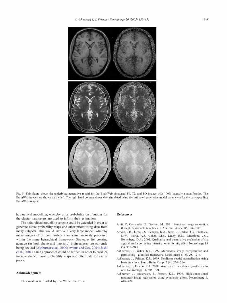
Fig. 3. This figure shows the underlying generative model for the BrainWeb simulated T1, T2, and PD images with 100% intensity nonuniformity. The

BrainWeb images are shown on the left. The right hand column shows data simulated using the estimated generative model parameters for the corresponding

BrainWeb images.


heirarchical modelling, whereby prior probability distributions for

the cluster parameters are used to inform their estimation.

The heirarchical modelling scheme could be extended in order to

generate tissue probability maps and other priors using data from

many subjects. This would involve a very large model, whereby

many images of different subjects are simultaneously processed

within the same heirarchical framework. Strategies for creating

average (in both shape and intensity) brain atlases are currently

being devised (Ashburner et al., 2000; Avants and Gee, 2004; Joshi

et al., 2004). Such approaches could be refined in order to produce

average shaped tissue probability maps and other data for use as

priors.

Acknowledgment

This work was funded by the Wellcome Trust.

References

Amit, Y., Grenander, U., Piccioni, M., 1991. Structural image restoration

through deformable templates. J. Am. Stat. Assoc. 86, 376–387.

Arnold, J.B., Liow, J.S., Schaper, K.A., Stern, J.J., Sled, J.G., Shattuck,

D.W., Worth, A.J., Cohen, M.S., Leahy, R.M., Mazziotta, J.C.,

Rottenberg, D.A., 2001. Qualitative and quantitative evaluation of six

algorithms for correcting intensity nonuniformity effect. NeuroImage 13

(5), 931–943.

Ashburner, J., Friston, K.J., 1997. Multimodal image coregistration and

partitioning—a unified framework. NeuroImage 6 (3), 209–217.

Ashburner, J., Friston, K.J., 1999. Nonlinear spatial normalization using

basis functions. Hum. Brain Mapp. 7 (4), 254–266.

Ashburner, J., Friston, K.J., 2000. Voxel-based morphometry—the meth-

ods. NeuroImage 11, 805–821.

Ashburner, J., Andersson, J., Friston, K.J., 1999. High-dimensional

nonlinear image registration using symmetric priors. NeuroImage 9,

619–628.


Ashburner, J., Andersson, J., Friston, K.J., 2000. Image registration using

a symmetric prior—in three-dimensions. Hum. Brain Mapp. 9 (4),

212–225.

Avants, B., Gee, J.C., 2004. Geodesic estimation for large deformation

anatomical shape averaging and interpolation. NeuroImage 23,

S139–S150.

Besag, J., 1986. On the statistical analysis of dirty pictures. J. R. Stat. Soc.,

B 48 (3), 259–302.

Bishop, C.M., 1995. Neural Networks for Pattern Recognition. Oxford

Univ. Press.

Bookstein, F.L., 1997. Landmark methods for forms without landmarks:

morphometrics of group differences in outline shape. Med. Image Anal.

1 (3), 225–243.

Bro-Nielsen, M., Gramkow, C., 1996. Fast fluid registration of medical

images. Lect. Notes Comput. Sci. 1131, 267–276.

Christensen, G.E., Rabbitt, R.D., Miller, M.I., Joshi, S.C., Grenander, U.,

Coogan, T.A., Van Essen, D.C., 1995. Topological properties of smooth

anatomic maps. In: Bizais, Y., Barillot, C., Di Paola, R. (Eds.), Proc.

Information Processing in Medical Imaging. Kluwer Academic Publish-

ers, Dordrecht, The Netherlands.

Christensen, G.E., Rabbitt, R.D., Miller, M.I., 1996. Deformable templates

using large deformation kinematics. IEEE Trans. Image Process. 5,

1435–1447.

Cocosco, C., Kollokian, V., Kwan, R.-S., Evans, A., 1997. Brainweb:

online interface to a 3D MRI simulated brain database. NeuroImage 5

(4), S425.

Collins, D.L., Peters, T.M., Evans, A.C., 1994. An automated 3D non-

linear image deformation procedure for determination of gross

morphometric variability in human brain. Proc. Visualization in

Biomedical Computing.

Collins, D.L., Evans, A.C., Holmes, C., Peters, T.M., 1995. Automatic 3D

segmentation of neuro-anatomical structures from MRI. In: Bizais, Y.,

Barillot, C., Di Paola, R. (Eds.), Proc. Information Processing in

Medical Imaging. Kluwer Academic Publishers, Dordrecht, The

Netherlands.

Collins, D., Zijdenbos, A., Kollokian, V., Sled, J., Kabani, N., Holmes,

C., Evans, A., 1998. Design and construction of a realistic digital

brain phantom. IEEE Trans. Med. Imaging 17 (3), 463–468.

D’Agostino, E., Maes, F., Vandermeulen, D., Suetens, P., 2004. Non-rigid

atlas-to-image registration by minimization of class-conditional image

entropy. In: Barillot, C., Haynor, D., Hellier, P. (Eds.), Proc. MICCAI

2004. LNCS 3216. Springer-Verlag, Berlin Heidelberg.

Davatzikos, C., 1996. Spatial normalization of 3D images using deformable

models. J. Comput. Assist. Tomogr. 20 (4), 656–665.

Dempster, A.P., Laird, N.M., Rubin, D.B., 1977. Maximum Likelihood

From Incomplete Data Via the EM Algorithm.

Edwards, P.J., Hill, D.L.G., Hawkes, D.J., 1997. Image guided interven-

tions using a three component tissue deformation model. Proc. Medical

Image Understanding and Analysis.

Evans, A.C., 1995. Commentary. Hum. Brain Mapp. 2, 165–189.

Evans, A.C., Kamber, M., Collins, D.L., Macdonald, D., 1994. An

MRIbased probabilistic atlas of neuroanatomy. In: Shorvon, S., Fish,

D., Andermann, F., Bydder, G.M., S.H. (Eds.), Magnetic Resonance

Scanning and Epilepsy, NATO ASI Ser., Ser. A: Life Sci., vol. 264.

Plenum Press, pp. 263–274.

Fischl, B., Salat, D.H., Busa, E., Albert, M., Dieterich, M., Haselgrove, C.,

van der Kouwe, A., Killiany, R., Kennedy, D., Klaveness, S., Montillo,

A., Makris, N., Rosen, B., Dale, A.M., 2002. Whole brain segmenta-

tion: automated labeling of neuroanatomical structures in the human

brain. Neuron 33, 341–355.

Fischl, B., Salat, D.H., van der Kouwe, A., Makris, N., Segonne, F.,

Quinn, B.T., Dale, A.M., 2004. Sequence-independent segmentation

of magnetic resonance images. NeuroImage 23, S69–S84.

Fissell, K., Tseytlin, E., Cunningham, D., Carter, C.S., Schneider, W.,

Cohen, J.D., 2003. Fiswidgets: a graphical computing environment

for neuroimaging analysis. Neuroinformatics 1 (1), 111–125.

Friston, K.J., Ashburner, J., Frith, C.D., Poline, J.-B., Heather, J.D.,

Frackowiak, R.S.J., 1995. Spatial registration and normalization of

images. Hum. Brain Mapp. 2, 165–189.

Garza-Jinich, M., Yanez, O., Medina, V., Meer, P., 1999. Automatic

correction of bias field in magnetic resonance images. Proc Interna-

tional Conference on Image Analysis and Processing.

Gee, J.C., Haynor, D.R., Le Briquer, L., Bajcsy, R.K., 1997. Advances in

elastic matching theory and its implementation. In: Cinquin, P., Kikinis,

R., Lavallee, S. (Eds.), Proc. CVRMed-MRCAST97. Springer-Verlag,Heidelberg.

Good, C.D., Johnsrude, I.S., Ashburner, J., Henson, R.N.A., Friston, K.J.,

Frackowiak, R.S.J., 2001. A voxel-based morphometric study of ageing

in 465 normal adult human brains. NeuroImage 14, 21–36.

Hellier, P., Barillot, C., Corouge, I., Gibaud, B., Le Goualher, G., Collins,

D.L., Evans, A.C., Malandain, G., Ayache, N., 2001. Retrospective

evaluation of inter-subject brain registration. In: Niessen, W.J.,

Viergever, M.A. (Eds.), MIUA. Springer, Utrecht, The Netherlands.

Hellier, P., Ashburner, J., Corouge, I., Barillot, C., Friston, K.J., 2002. Inter

subject registration of functional and anatomical data using spm.

Medical Image Computing and Computer Assisted Intervention 2002,

MICCAIT02, LNCS 2489 (Tokyo).

Joshi, S.C., Miller, M.I., 2000. Landmark matching via large deforma-

tion diffeomorphisms. IEEE Transactions on Medical Imaging 9 (8),

1357–1370.

Joshi, S., Davis, B., Jomier, M., Gerig, G., 2004. Unbiased diffeomor-

phic atlas construction for computational anatomy. NeuroImage 23,

S151–S160.

Kwan, R.K.-S., Evans, A.C., Pike, G.B., 1996. An extensible MRI

simulator for post-processing evaluation. Proc. Visualization in Bio-

medical Computing.

Kybic, J., Unser, M., 2003. Fast parametric elastic image registration. IEEE

Trans. Med. Imaging 12 (11), 1427–1442.

Laidlaw, D.H., Fleischer, K.W., Barr, A.H., 1998. Partial-volume Bayesian

classification of material mixtures in MR volume data using voxel

histograms. IEEE Trans. Med. Imaging 17 (1), 74–86.

Likar, B., Viergever, M.A., Pernus, F., 2001. Retrospective correction of

MR intensity inhomogeneity by information minimization. IEEE Trans.

Med. Imaging 20 (12), 1398–1410.

MacDonald, D., Kabani, N., Avis, D., Evans, A.C., 2000. Automated 3-d

extraction of inner and outer surfaces of cerebral cortex from MRI.

NeuroImage 12, 340–356.

Mangin, J.-F., 2000. Entropy minimization for automatic correction of

intensity nonuniformity. Proc. IEEE Workshop on Mathematical

Methods in Biomedical Image Analysis.

Miller, M.I., 2004. Computational anatomy: shape, growth, and

atrophy comparison via diffeomorphisms. NeuroImage 23, S19–S33.

Miller, M., Younes, L., 2001. Group actions, homeomorphisms, and

matching: a general framework. Int. J. Comput. Vis. 41 (1), 61–84.

Miller, M.I., Christensen, G.E., Amit, Y., Grenander, U., 1993. Mathemat-

ical textbook of deformable neuroanatomies. Proc. Natl. Acad. Sci. 90,

11944–11948.

Miller, M., Banerjee, A., Christensen, G., Joshi, S., Khaneja, N., 1997.

Statistical methods in computational anatomy. Stat. Methods Med. Res.

6, 267–299.

Neal, R.M., Hinton, G.E., 2004. A view of the EM algorithm that justifies

incremental, sparse, and other variants. In: Jordan, M.I. (Ed.), Learning

in Graphical Model.

Pham, D.L., Prince, J.L., 1999. Adaptive fuzzy segmentation of magnetic

resonance images. IEEE Trans. Med. Imaging 18 (9), 737–752.

Pitiot, A., Delingette, H., Thompson, P.M., Ayache, N., 2004. Expert

knowledge-guided segmentation system for brain MRI. NeuroImage 23,

S85–S96.

Press, W.H., Teukolsky, S.A., Vetterling, W.T., Flannery, B.P., 1992.

Numerical Recipes in C. Second edition. Cambridge, Cambridge.

Rex, D.E., Maa, J.Q., Toga, A.W., 2003. The LONI pipeline processing

environment. NeuroImage 19 (3), 1033–1048.

Rueckert, D., Sonoda, L.I., Hayes, C., Hill, D.L.G., Leachand, M.O.,

Hawkes, D.J., 1999. Nonrigid registration using free-form deforma-


tions: application to breast MR images. IEEE Trans. Med. Imaging 18

(8), 712–721.

Shattuck, D.W., Sandor-Leahy, S.R., Schaper, K.A., Rottenberg, D.A.,

Leahy, R.M., 2001. Magnetic resonance image tissue classification

using a partial volume model. NeuroImage 13 (5), 856–876.

Shepp, L.A., Vardi, Y., 1982. Maximum likelihood reconstruction in

positron emission tomography. IEEE Trans. Med. Imaging 1, 113–122.

Sled, J.G., Zijdenbos, A.P., Evans, A.C., 1998. A non-parametric method

for automatic correction of intensity non-uniformity in MRI data. IEEE

Trans. Med. Imaging 17 (1), 87–97.

Studholme, C., Cardenas, V., Song, E., Ezekiel, F., Maudsley, A., Weiner,

M., 2004. Accurate template-based correction of brain MRI intensity

distortion with application to dementia and aging. IEEE Trans. Med.

Imaging 23 (1), 99–110.

Styner, M., 2000. Parametric estimate of intensity inhomogeneities applied

to MRI. IEEE Trans. Med. Imaging 19 (3), 153–165.

Thevenaz, P., Unser, M., 2000. Optimization of mutual information for

multiresolution image registration. IEEE Trans. Image Process. 9 (12),

2083–2099.

Thevenaz, P., Blu, T., Unser, M., 2000. Interpolation revisited. IEEE Trans.

Med. Imaging 19 (7), 739–758.

Thirion, J.-P., 1995. Fast non-rigid matching of 3D medical images. Tech.

Rep. 2547, Institut National de Recherche en Informatique et en

Automatique. Available from http://www.inria.fr/rrrt/rr-2547.html.

Tohka, J., Zijdenbos, A., Evans, A., 2004. Fast and robust parameter

estimation for statistical partial volume models in brain MRI. Neuro-

Image 23, 84–97.

Unser, M., Aldroubi, A., Eden, M., 1993a. B-spline signal processing: Part

I—theory. IEEE Trans. Signal Process. 41 (2), 821–833.

Unser, M., Aldroubi, A., Eden, M., 1993b. B-spline signal processing: Part

II—efficient design and applications. IEEE Trans. Signal Process. 41

(2), 834–848.

Vaillant, M., Miller, M., Younes, L., Trouve, A., 2004. Statistics on

diffeomorphisms via tangent space representations. NeuroImage 23,

S161–S169.

Van Leemput, K., Maes, F., Vandermeulen, D., Suetens, P., 1999a.

Automated model-based bias field correction of MR images of the

brain. IEEE Trans. Med. Imaging 18 (10), 885–896.

Van Leemput, K., Maes, F., Vandermeulen, D., Suetens, P., 1999b.

Automated model-based tissue classification of MR images of the

brain. IEEE Trans. Med. Imaging 18 (10), 897–908.

Van Leemput, K., Maes, F., Vandermeulen, D., Suetens, P., 2001. A

statistical framework for partial volume segmentation. In: Niessen, W.,

Viergever, M. (Eds.), Proc. MICCAI 2001. LNCS 2208. Springer-

Verlag, Heidelberg.

Wells III, W.M., Grimson, W.E.L., Kikinis, R., Jolesz, F.A., 1996a.

Adaptive segmentation of MRI data. IEEE Trans. Med. Imaging 15

(4), 429–442.

Wells III, W.M., Viola, P., Atsumi, H., Nakajima, S., Kikinis, R., 1996b.

Multi-modal volume registration by maximisation of mutual informa-

tion. Med. Image Anal. 1 (1), 35–51.

Woods, R.P., 2003. Characterizing volume and surface deformations in an

atlas framework: theory, applications, and implementation. NeuroImage

18 (3), 769–788.

Woods, R.P., Grafton, S.T., Holmes, C.J., Cherry, S.R., Mazziotta, J.C.,

1998a. Automated image registration: I. General methods and intra-

subject, intramodality validation. J. Comput. Assist. Tomogr. 22 (1),

139–152.

Woods, R.P., Grafton, S.T., Watson, J.D.G., Sicotte, N.L., Mazziotta,

J.C., 1998b. Automated image registration: II. Intersubject validation

of linear and nonlinear models. J. Comput. Assist. Tomogr. 22 (1),

153–165.

Xiaohua, C., Brady, M., Rueckert, D., 2004. Simultaneous segmentation

and registration for medical image. In: Barillot, C., Haynor, D., Hellier,

P. (Eds.), Proc. MICCAI 2004. LNCS 3216. Springer-Verlag, Berlin

Heidelberg.

Zhang, Y., Brady, M., Smith, S., 2001. Segmentation of brain MR images

through a hidden Markov Random Field model and the expectation–

maximization algorithm. IEEE Trans. Med. Imaging 20 (1), 45–57.

Zijdenbos, A.P., Forghani, R., Evans, A.C., 2002. Automatic bpipelineQanalysis of 3-D MRI data for clinical trials: application to multiple

sclerosis. IEEE Trans. Med. Imaging 21 (10), 1280–1291.

http:\\www.inria.fr

unified segmentation - fil | ucl

Documents