unit 12: analysis of single factor experiments -...
TRANSCRIPT
7/16/2004 Unit 12 - Stat 571 - Ramón V. León 1
Unit 12: Analysis of Single Factor Experiments
Statistics 571: Statistical MethodsRamón V. León
7/16/2004 Unit 12 - Stat 571 - Ramón V. León 2
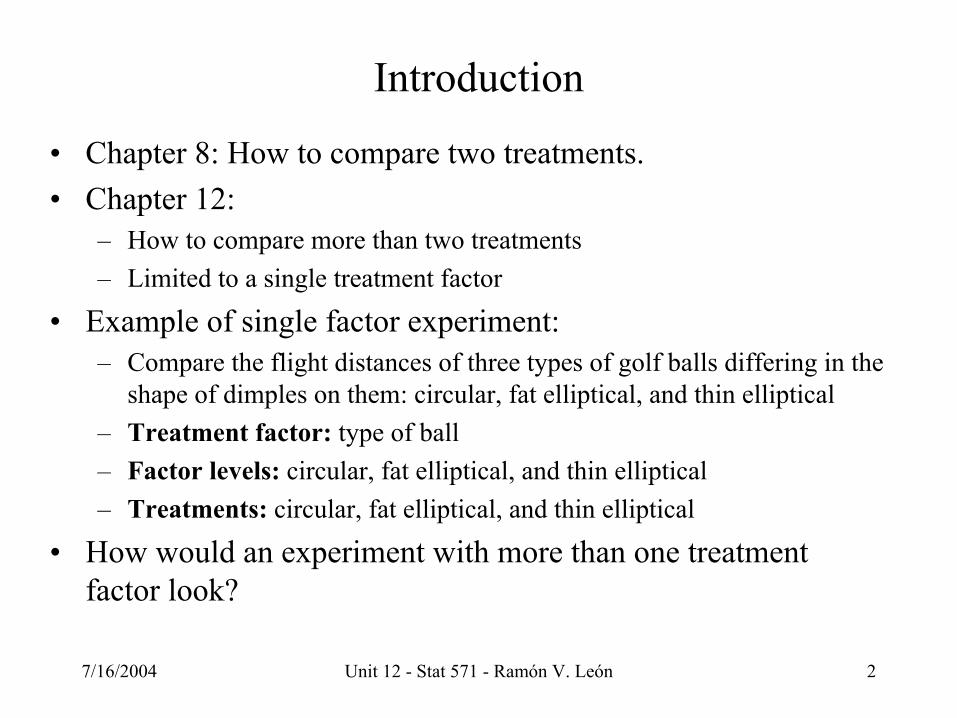
Introduction
• Chapter 8: How to compare two treatments.• Chapter 12:
– How to compare more than two treatments– Limited to a single treatment factor
• Example of single factor experiment:– Compare the flight distances of three types of golf balls differing in the
shape of dimples on them: circular, fat elliptical, and thin elliptical– Treatment factor: type of ball– Factor levels: circular, fat elliptical, and thin elliptical– Treatments: circular, fat elliptical, and thin elliptical
• How would an experiment with more than one treatment factor look?

7/16/2004 Unit 12 - Stat 571 - Ramón V. León 3
Experimental Designs
RandomizedBlock Design
Matched Pair Design
Dependent Samples
Completely Randomized Design
Independent Samples Design
Independent Samples
More Than Two Treatments
Two Treatments

7/16/2004 Unit 12 - Stat 571 - Ramón V. León 4
Completely Randomized Design
Random sample drawn in each of six molding stations.Runs should be in random order to protect against time trend

7/16/2004 Unit 12 - Stat 571 - Ramón V. León 5
Completely Randomized Design Notation
1
a
ij
N n=
= ∑
If the sample sizes are equalthe design is balanced;otherwise thedesign is unbalanced
7/16/2004 Unit 12 - Stat 571 - Ramón V. León 6
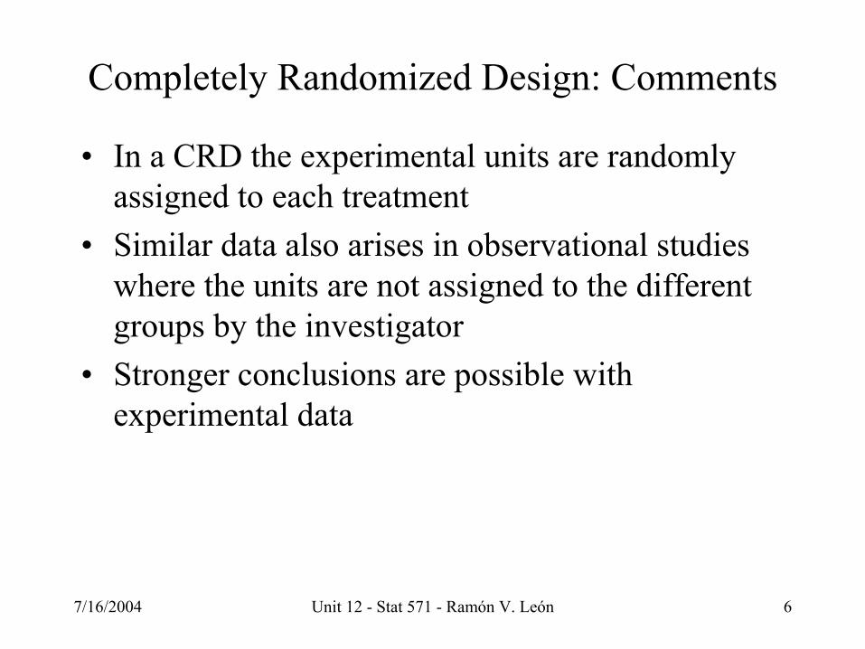
Completely Randomized Design: Comments
• In a CRD the experimental units are randomly assigned to each treatment
• Similar data also arises in observational studies where the units are not assigned to the different groups by the investigator
• Stronger conclusions are possible with experimental data
7/16/2004 Unit 12 - Stat 571 - Ramón V. León 7
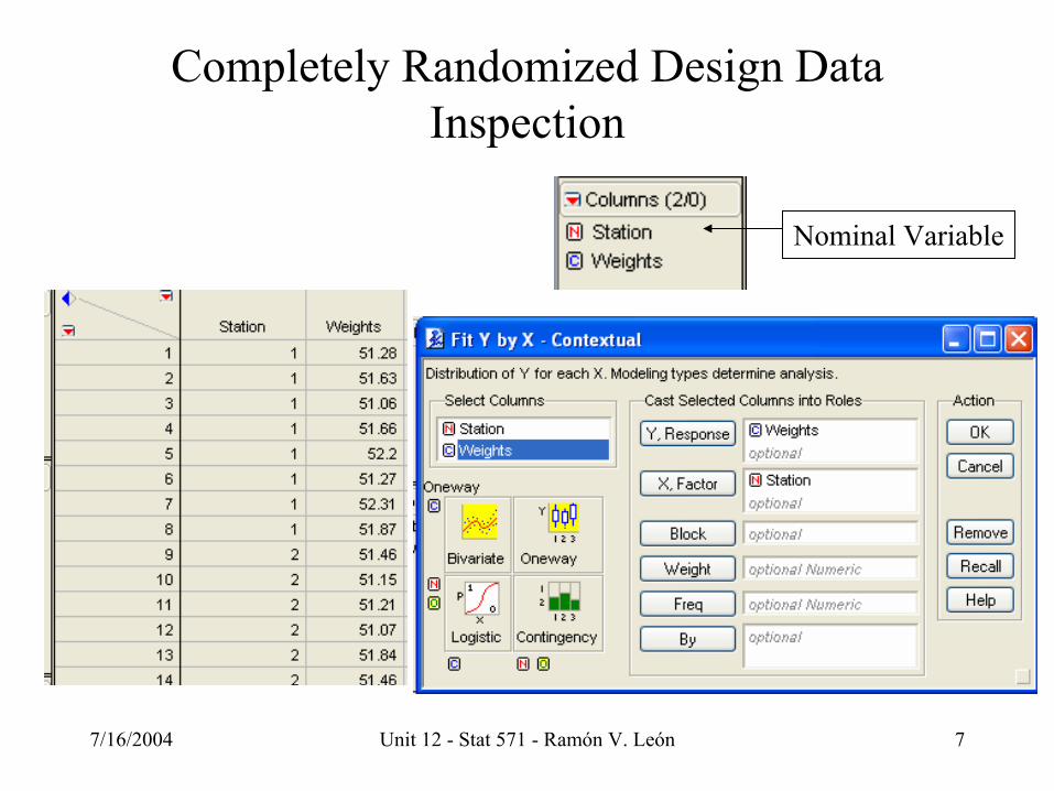
Completely Randomized Design Data Inspection
Nominal Variable

7/16/2004 Unit 12 - Stat 571 - Ramón V. León 8
CRD Side-by-Side Box Plots
Wei
ghts
51
51.5
52
52.5
1 2 3 4 5 6
Station
Station 5 has twooutliers
Stations 4, 5, and 6which are suppliedby feeder 2 have a higher average as a group thanstations 1, 2, and 3that are supplied byfeeder 1. Is this difference realor the resultsampling variation?
7/16/2004 Unit 12 - Stat 571 - Ramón V. León 9
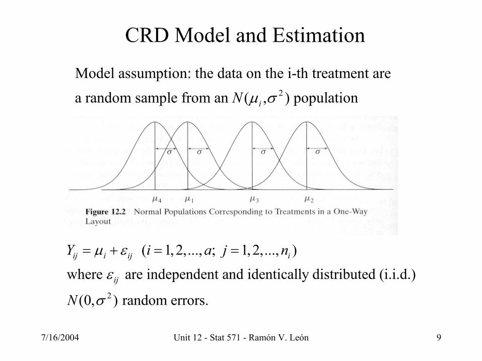
CRD Model and Estimation
2
Model assumption: the data on the i-th treatment are a random sample from an ( , ) population iN µ σ
2
( 1, 2,..., ; 1, 2,..., )
where are independent and identically distributed (i.i.d.)
(0, ) random errors.
ij i ij i
ij
Y i a j n
N
µ ε
ε
σ
= + = =

7/16/2004 Unit 12 - Stat 571 - Ramón V. León 10
CRD Model and Estimation2
iThe treatment means and the error variance are unknown parameters. The primary interest is on comparing the means
µ σ
i
11
1
i
Frequently, we write where is the "grand mean"defined as the weighted average of the :
if are egual
and is the deviation of the i-th treatment
i i
aai i ii i
iaii
i
nn n
an
µ µ τ µµ
µµµ
τ µ µ
==
=
= +
= = =
= −
∑∑∑
i
meanfrom this grand mean.We refer to as the i-th treatment effect.τ
7/16/2004 Unit 12 - Stat 571 - Ramón V. León 11
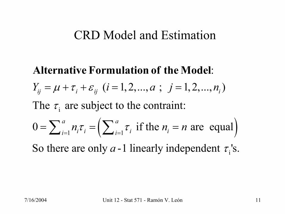
CRD Model and Estimation
( )i
1 1
i
:( 1, 2,..., ; 1, 2,..., )
The are subject to the contraint:
0 if the are equal
So there are only -1 linearly independent '
ij i ij i
a ai i i ii i
Y i a j n
n n n
a
µ τ ε
τ
τ τ
τ= =
= + + = =
= = =∑ ∑
Alternative Formulation of the Model
s.
7/16/2004 Unit 12 - Stat 571 - Ramón V. León 12
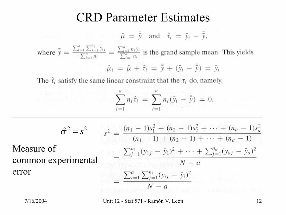
CRD Parameter Estimates
2 2ˆ sσ =
Measure of common experimentalerror

7/16/2004 Unit 12 - Stat 571 - Ramón V. León 13
ANOVA in JMP’s Fit Model Platform
Note that the Station variable is nominal
7/16/2004 Unit 12 - Stat 571 - Ramón V. León 14
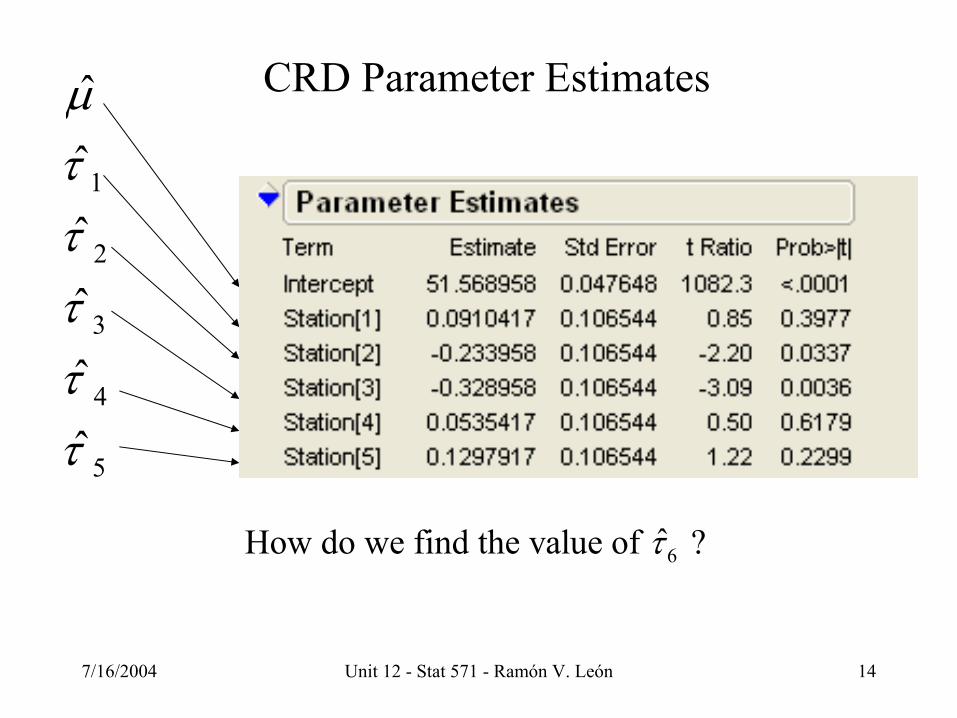
CRD Parameter Estimates
1
2
3
4
5
ˆˆˆˆˆˆ
µτττττ
6ˆHow do we find the value of ?τ
2s

7/16/2004 Unit 12 - Stat 571 - Ramón V. León 15
Relationship to Dummy Variable Regression
1 2 3 4 5
1 1 2 2 3 3
1 if station i
1 if station 6 0 otherwise
1, 2,...,5
51.57 0.09 0.23 0.33 0.05 0.13ˆ ˆ ˆ ˆ ˆ
iz
i
y z z z z zy z z z
εµ τ τ τ τ
= −
=
= + − − + + +
= + + + + 4 4 5 5ˆz zτ ε+ +

7/16/2004 Unit 12 - Stat 571 - Ramón V. León 16
CRD Parameter Estimates
2s
7/16/2004 Unit 12 - Stat 571 - Ramón V. León 17
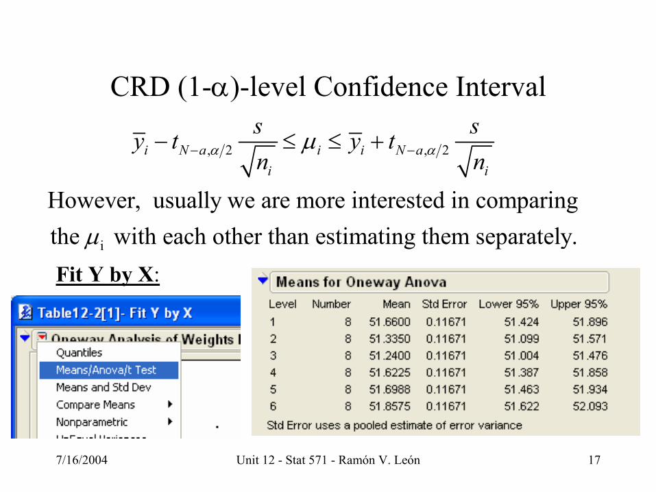
CRD (1-α)-level Confidence Interval
, 2 , 2
i
However, usually we are more interested in comparingthe with each other than estimating them separately.
i N a i i N ai i
s sy t y tn nα αµ
µ
− −− ≤ ≤ +
Fit Y by X:
7/16/2004 Unit 12 - Stat 571 - Ramón V. León 18
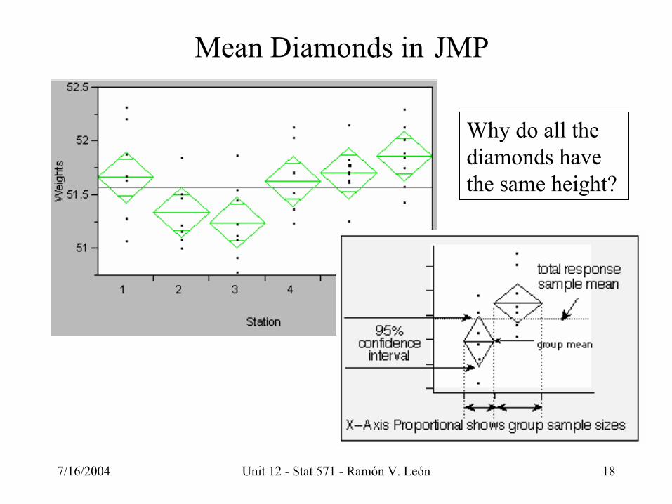
Mean Diamonds in JMP
Why do all the diamonds have the same height?
7/16/2004 Unit 12 - Stat 571 - Ramón V. León 19
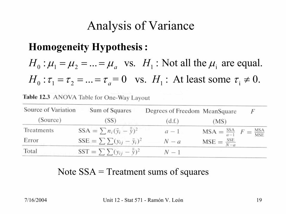
Analysis of Variance
0 1 2 1 i
0 1 2 1 i
: ... vs. : Not all the are equal.: ... = 0 vs. : At least some 0.
a
a
H HH H
µ µ µ µτ τ τ τ
= = =
= = = ≠
Homogeneity Hypothesis :
Note SSA = Treatment sums of squares

7/16/2004 Unit 12 - Stat 571 - Ramón V. León 20
ANOVA in JMPWrong ANOVA table:
Correct ANOVA table:
Note that the SS has the wrong number of degrees of freedom
0 1(Model: )Y Stationβ β ε= + +
1 1 2 2 3 3 4 4 5 5(Model: )Y z z z z zµ τ τ τ τ τ ε= + + + + + +
7/16/2004 Unit 12 - Stat 571 - Ramón V. León 21
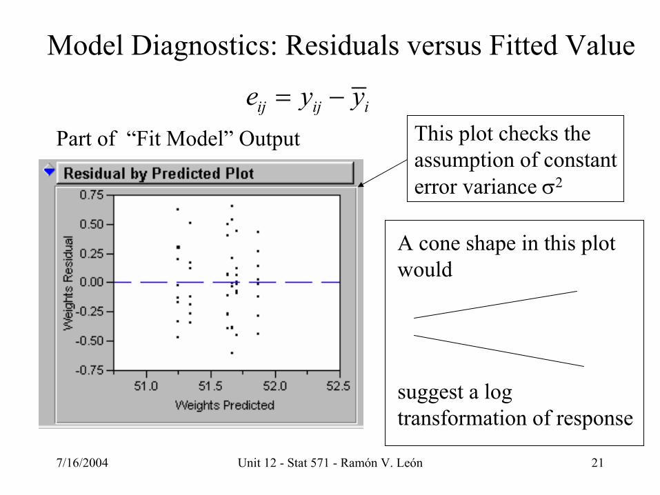
Model Diagnostics: Residuals versus Fitted Value
ij ij ie y y= −Part of “Fit Model” Output This plot checks the
assumption of constanterror variance σ2
A cone shape in this plot would
suggest a logtransformation of response
7/16/2004 Unit 12 - Stat 571 - Ramón V. León 22
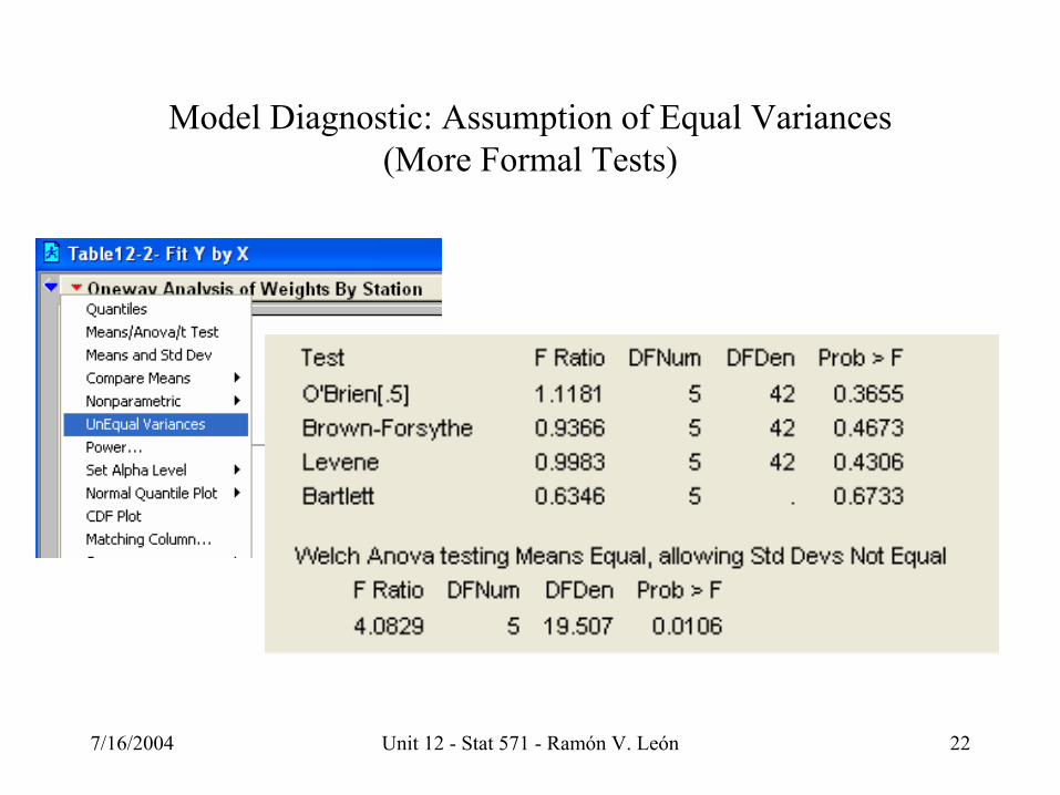
Model Diagnostic: Assumption of Equal Variances (More Formal Tests)
7/16/2004 Unit 12 - Stat 571 - Ramón V. León 23
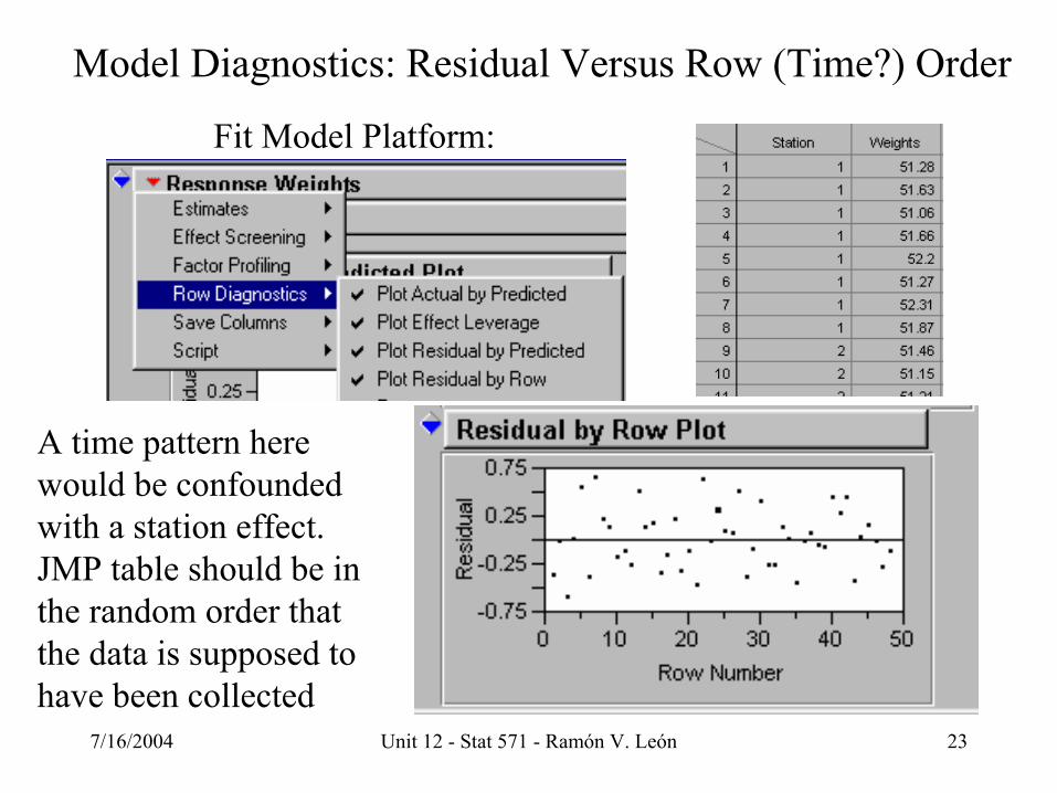
Model Diagnostics: Residual Versus Row (Time?) Order
A time pattern here would be confounded with a station effect. JMP table should be in the random order that the data is supposed to have been collected
Fit Model Platform:

7/16/2004 Unit 12 - Stat 571 - Ramón V. León 24
Model Diagnostics: Normal Plot of Residuals
Strong indication that errors are normallydistributed.

7/16/2004 Unit 12 - Stat 571 - Ramón V. León 25
Multiple Comparison of Means
0 1If : ... is rejected all that we can say is thatthe treatment means are not equal. The -test does not pinpoint which treatment means are significantly differentfrom each other.We could test al
aHF
µ µ= =
( )
0
0 , 2
, 2
l :| |
Reject if 1 1
| | 1 1
Least significant difference, LSD
ij i j
i jij ij N a
i j
i j N a i j
Hy y
H t ts n n
y y t s n n
α
α
µ µ
−
−
=
−= >
+
⇔ − > + =
pairwise equality hypotheses

7/16/2004 Unit 12 - Stat 571 - Ramón V. León 26
Pairwise Equality Hypotheses
Since each of the 15 pairwise test have a level α, the type I errorprobability of declaring at least one pairwise differencefalsely significant will exceed α.
Family Wise Error rate (FWE):FWE = P{Reject at least one true null hypothesis when they are true}
If all six means are actually equal in the plastic container exampleFWE = 0.350 when each LSD test is done at the 0.05 level.
Fisher’s protected LSD method:Use LSD method only after the F-test rejects(This method is not recommended today.)
7/16/2004 Unit 12 - Stat 571 - Ramón V. León 27
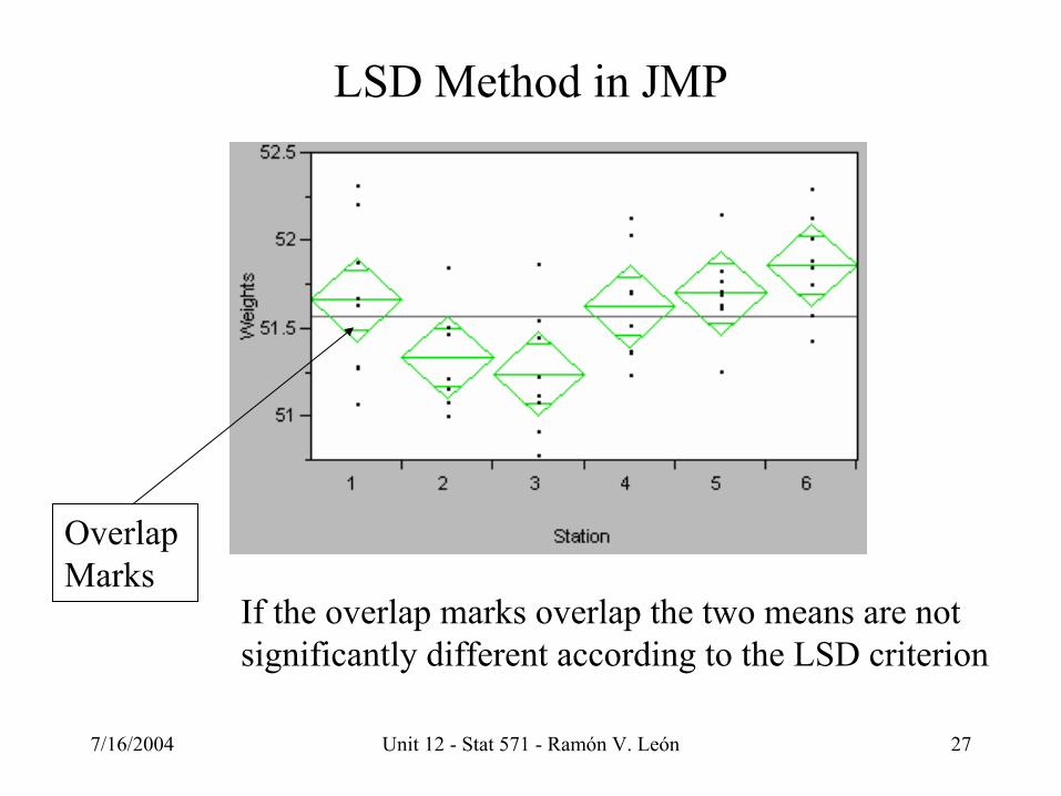
LSD Method in JMP
Overlap Marks
If the overlap marks overlap the two means are notsignificantly different according to the LSD criterion
7/16/2004 Unit 12 - Stat 571 - Ramón V. León 28
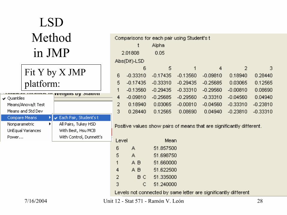
LSD Method in JMP
Fit Y by X JMP platform:
7/16/2004 Unit 12 - Stat 571 - Ramón V. León 29
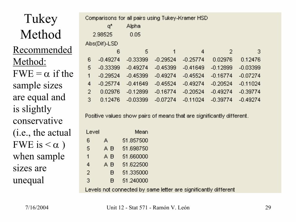
TukeyMethod
Recommended Method:FWE = α if the sample sizes are equal and is slightly conservative(i.e., the actual FWE is < α ) when sample sizes are unequal
7/16/2004 Unit 12 - Stat 571 - Ramón V. León 30
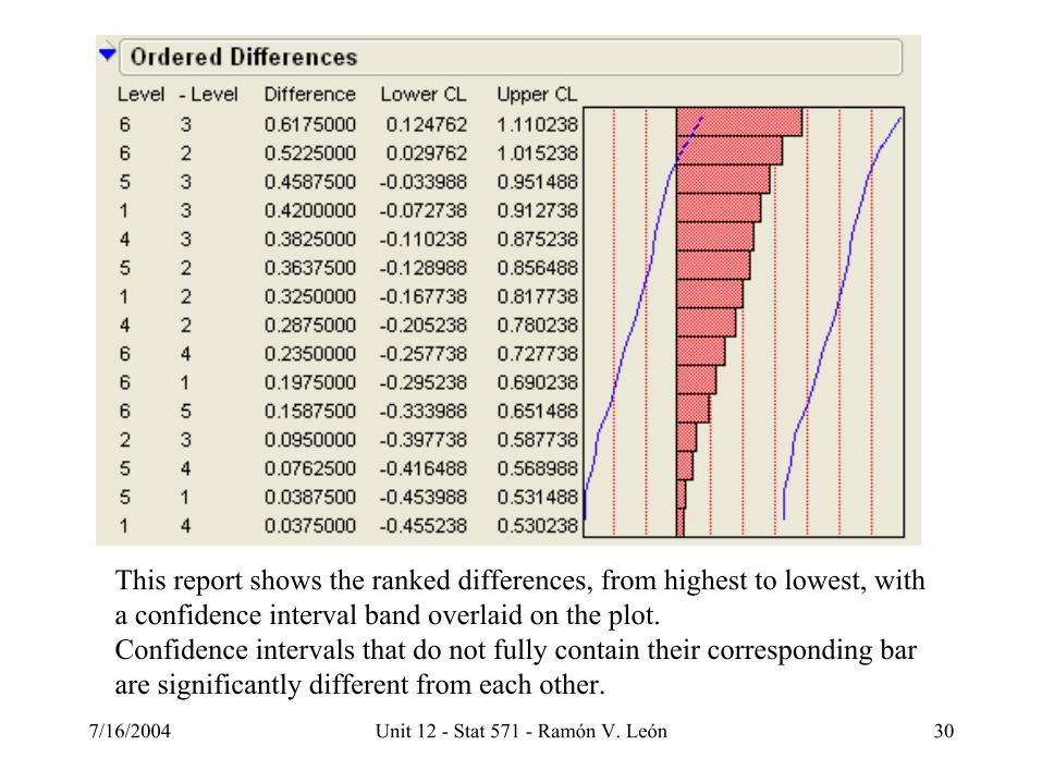
This report shows the ranked differences, from highest to lowest, with a confidence interval band overlaid on the plot. Confidence intervals that do not fully contain their corresponding bar are significantly different from each other.

7/16/2004 Unit 12 - Stat 571 - Ramón V. León 31
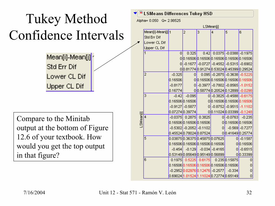
Tukey Method Confidence IntervalsThis is a way of construction 100(1-α)% Simultaneous Confidence Intervals(SCIs) for all pairwise difference of means
7/16/2004 Unit 12 - Stat 571 - Ramón V. León 32
Tukey Method Confidence Intervals
Compare to the Minitab output at the bottom of Figure 12.6 of your textbook. How would you get the top output in that figure?

7/16/2004 Unit 12 - Stat 571 - Ramón V. León 33
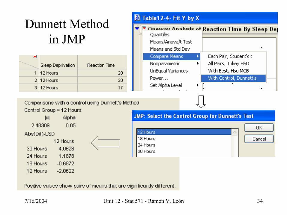
Dunnett Method for Comparisons with a Control
7/16/2004 Unit 12 - Stat 571 - Ramón V. León 34
Dunnett Method in JMP
7/16/2004 Unit 12 - Stat 571 - Ramón V. León 35
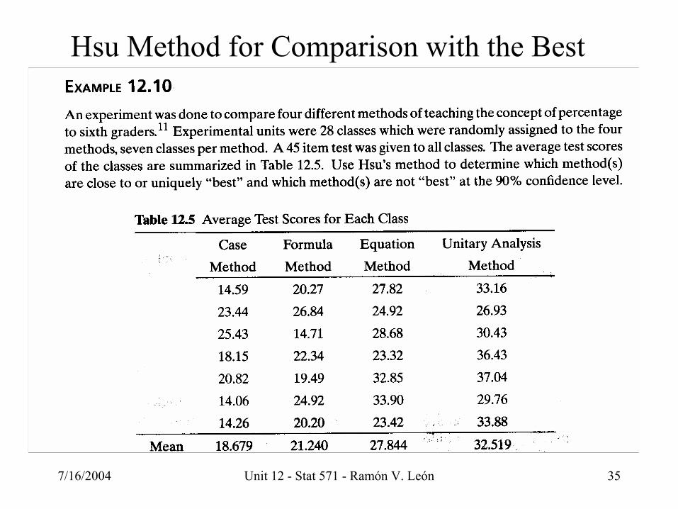
Hsu Method for Comparison with the Best

7/16/2004 Unit 12 - Stat 571 - Ramón V. León 36
Test
Sco
re
10
15
20
25
30
35
40
Case Equation Formula Unitary Analysis
Method
Box Plots for Teaching Method

7/16/2004 Unit 12 - Stat 571 - Ramón V. León 37
Hsu Method in JMP
Explanation Next Page

7/16/2004 Unit 12 - Stat 571 - Ramón V. León 38
Hsu Method in JMP
The UnitaryMethod is best
Can’t tell which is the worse method

7/16/2004 Unit 12 - Stat 571 - Ramón V. León 39
Randomized Block Design•Blocking helps to reduce experimental error variation caused bydifference in the experimental units by grouping them into homogeneous sets (called blocks).
•Treatments are randomly assigned within each block

7/16/2004 Unit 12 - Stat 571 - Ramón V. León 40
Randomized Block Design Model: Fixed Block Effects
2
i
j
bj 1 j = 1
( 1,..., ; 1,..., )
where are i.i.d. N(0, ) is called the grand meanis called the th treatment effect is called the th block effect
0 and 0 so there are
ij i j ij
ij
aii
Y i a j b
ij
µ τ β ε
ε σ
µτβ
τ β=
= + + + = =
= =∑ ∑1 independent treatment effects
-1 independent block effectsab
−

7/16/2004 Unit 12 - Stat 571 - Ramón V. León 41
“Mystery of Degrees of Freedom Explained”
Counting the grand mean there are 1 ( -1) ( -1) 1unknown parameters. (This many degrees of freedom are neededto estimate these parameters.)There are observations (total degrees of freedom).So
a b a b
N ab
+ + = + −
= there are ( 1) ( 1)( 1) degrees of
freedom for estimating the error variation(degrees of freedom for error).
ab a b a bν = − + − = − −

7/16/2004 Unit 12 - Stat 571 - Ramón V. León 42
No Interactions Between Treatments and Blocks
The difference in mean responses between any two treatmentsis the same across all blocks
' ' '( ) ( )
which is indepedent of the particular block jij i j i j i j i iµ µ µ τ β µ τ β τ τ− = + + − + + = −
Example: Consider the treatments to be fertilizer and the blocks to be different fields. Then no interaction implies that the differencein mean yields between any two fertilizers is the same for all fields.
We say that there are no interactions between treatments and blocks
7/16/2004 Unit 12 - Stat 571 - Ramón V. León 43
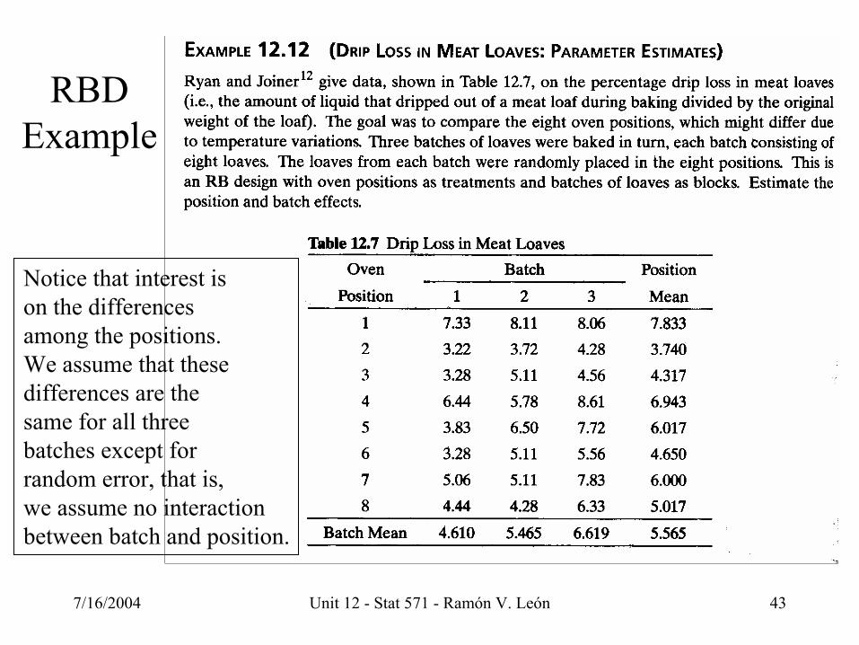
RBD Example
Notice that interest is on the differences among the positions. We assume that these differences are the same for all three batches except for random error, that is,we assume no interactionbetween batch and position.

7/16/2004 Unit 12 - Stat 571 - Ramón V. León 44
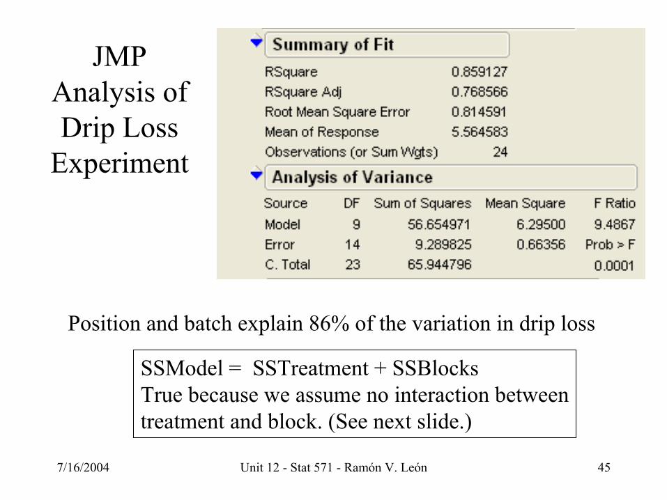
JMP Analysis of Drip Loss Experiment
Nominal
7/16/2004 Unit 12 - Stat 571 - Ramón V. León 45
JMP Analysis of Drip Loss
Experiment
Position and batch explain 86% of the variation in drip loss
SSModel = SSTreatment + SSBlocksTrue because we assume no interaction betweentreatment and block. (See next slide.)

7/16/2004 Unit 12 - Stat 571 - Ramón V. León 46
JMP 4 Analysis of Drip Loss Experiment. III
Model SS = 56.654971
These two tablewere not thesame in regression.They are equal herebecause the modelis balanced.
Also in regressionthe sum of the TypeIII sums of squares is not equal to the model sumsof squares. This only true here becausethe model is balanced.
(Type III)
Recall: The sum of the Type I sums of squares is always equal to the model sums of squares
The P-values show that there are significant position effects. We recommend ignoring the Block (Batch) test because it is not meaningful for the RBD.

7/16/2004 Unit 12 - Stat 571 - Ramón V. León 47
Drip Loss in Meat Loaves: Residual Plots
The predicted versus residual plot is partof the standard output of the Fit Modelplatform. The normal plot was obtainedby saving the residuals and then going tothe Distribution platform.
7/16/2004 Unit 12 - Stat 571 - Ramón V. León 48
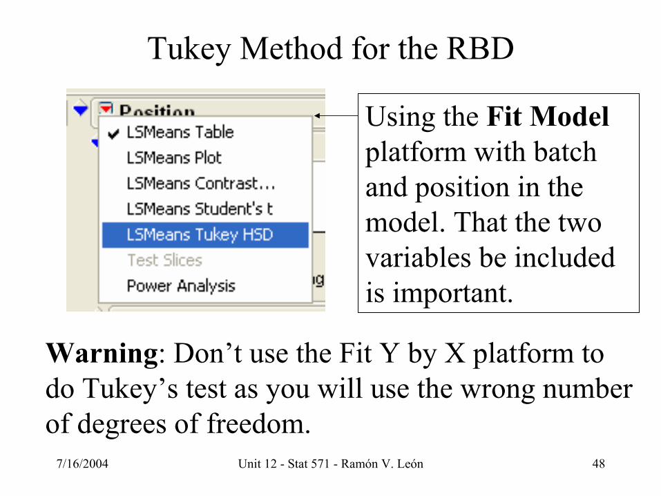
Tukey Method for the RBD
Warning: Don’t use the Fit Y by X platform to do Tukey’s test as you will use the wrong number of degrees of freedom.
Using the Fit Modelplatform with batch and position in the model. That the two variables be included is important.

7/16/2004 Unit 12 - Stat 571 - Ramón V. León 49
Tukey Method for the RBD

7/16/2004 Unit 12 - Stat 571 - Ramón V. León 50
Tukey Method for the RBD

7/16/2004 Unit 12 - Stat 571 - Ramón V. León 51
Mixed Effects Model for the RB Design
2
2B
i
j
1
( 1,..., ; 1,..., )
where are i.i.d. N(0, )
and are i.i.d. N(0, )
is called the grand mean is called the th treatment effect's are called the block effects
0 so
ij i j ij
ij
j
aii
Y i a j b
i
µ τ β ε
ε σ
β σ
µτβ
τ=
= + + + = =
=∑ there are 1 independent treatment effectsa −
Independent

7/16/2004 Unit 12 - Stat 571 - Ramón V. León 52
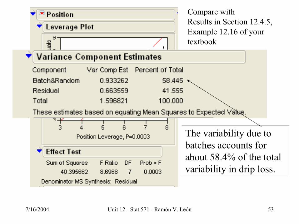
7/16/2004 Unit 12 - Stat 571 - Ramón V. León 53
Compare withResults in Section 12.4.5,Example 12.16 of your textbook
The variability due to batches accounts for about 58.4% of the total variability in drip loss.