universite paris-sud - theses.fr · universite paris-sud ecole doctorale: 534 mipege ... patrick...
TRANSCRIPT

UNIVERSITE PARIS-SUDECOLE DOCTORALE: 534 MIPEGE
Laboratoire: CERN
PHYSIQUE
THESE DE DOCTORATsoutenue le 21/11/2012 par
Aurelien MARSILI
Identification of LHC beam loss mechanism:
A deterministic treatment of loss patterns
Directeur de these : Patrick PUZO
Encadrante CERN : Eva Barbara HOLZER
Composition du jury :
President du jury : Achille STOCCHI
Rapporteurs : Mike LAMONT
Amor NADJI
Membre invite : Jacques MARRONCLE

ii

To Gen,
beacon of sanity in a storm of lunacy.

Acknowledgements
First of all, I would like to thank my girlfriend, Genevieve Steele, for helping
to convince me to start a PhD in the first place. Without her incentive, I
don’t think I would have even started.
Then, amongst the people who allowed this PhD to take place, such as
my section leader Bernd Dehning, I owe a lot to my university supervisor,
Pr. Patrick Puzo, for accepting me as a PhD student in addition to his
already busy schedule. He was the essential link between me and the uni-
versity, saved me from a lot of administrative work, and above all was there
for me every time I needed it. He was an excellent and reliable guidance for
a PhD; the kind of supervisor every PhD student whishes to have.
I would like to address a specific thank to my supervisor, Barbara Holzer.
She had the insight to let me test some of my ideas for sometimes several
days on, with no guarantee of positive results; most of the tools developed
for this PhD would have not existed without this freedom, and doing the
work would have been much harder. But I am also very grateful for the
many discussions of the results and the directions: every time a result was
described as “interesting”, I knew I was on the right path.
About one of these experiments, I am eternally beholden to my best friend
Olivier Pernet. Sometimes two days messing with the right thing with the
right people is worth more than an entire year of lessons. He made me
moved to Python, which multiplied both creativity and efficiency; I remain
convinced that none of this work would have been even possible without
that original help.
One a related note, I need to thank people that saved weeks of my work by
devoting to me half an hour of their time, by providing precise and efficient
advise; and amongst these people are, each one with their own specialty:

Jorg Wenninger, Rhodri Jones, Jean-Jacques Gras, and my colleagues Mar-
iusz Sapinski, Christos Zamantzas and Ewald Effinger.
The one person that helped me the most with all the technical details is
with no doubt Annika Nordt. She provided the most help, developing and
testing the new database access tool, and was the interface with the database
people. Chris Roderick and Ronny Billen deserve a specific thought, for
letting us mess with their databases, and for providing the access tools.
I would like to honor the memory of Shennong, the legendary Chinese em-
peror who discovered tea in 2737 BC. Without his discovery, and the massive
trade developed by the United Kingdom in the 18th century, none of this
work would have happened.
On a different note, I’d like to thank all my past and present office mates,
especially Christoph Kurfurst and Eduardo Nebot del Busto, for being such
nice company, quiet when I was working and ready for a break when I
needed it. I’ve never been so happy to go to work. This also includes my
“thesis brother” Mohamed Koujili, and his wisdom.
Finally, I would like to thank Gen again for sharing my life all this time, and
all the fun that was; for understanding the difficulties of a PhD by doing
one herself; and for being always there for me, reliable as ever.

iv

Summary
CERN’s Large Hadron Collider (LHC) is the largest device ever built, with a total
circumference of 26.7 km; and it is the most powerful accelerator ever, both in beam
energy and beam intensity. The main magnets are superconducting, and contain the
particles into two counter circulating beams which collide in four interaction points.
CERN and the LHC will be described in chap. 1
The superconducting magnets of the LHC have to be protected against particle
losses. Depending on the number of lost particles, the coils of the magnets could
become normal conducting and/or will be damaged. To avoid these events a beam
loss monitoring (BLM) system was installed to measure the particle loss rates. If the
predefined safe thresholds of loss rates are exceeded, the beams are directed out of the
accelerator ring towards the beam dump.
The detectors of the BLM system are mainly ionization chambers located outside of
the cryostats. In total, about 3600 ionisation chambers are installed. Further challenges
include the high dynamical range of losses (chamber currents ranging between 2 pA and
1 mA). The BLM system will be further described in chap. 2.
The subject of this thesis is to study the loss patterns and find the origin of the losses
in a deterministic way, by comparing measured losses to well understood loss scenarios.
This is done through a case study: different techniques were used on a restrained set of
loss scenarios, as a proof of concept of the possibility to extract information from a loss
profile. Finding the origin of the losses should allow acting in response. A justification
of the doctoral work will be given at the end of chap. 2.
This thesis will then focus on the theoretical understanding and the implementation
of the decomposition of a measured loss profile as a linear combination of the reference
v

scenarios; and the evaluation of the error on the recomposition and its correctness. The
principles of vector decomposition are developed in chap. 3.
An ensemble of well controlled loss scenarios (such as vertical and horizontal blow-
up of the beams or momentum offset during collimator loss maps) has been gathered,
in order to allow the study and creation of reference vectors. To achieve the Vector
Decomposition, linear algebra (matrix inversion) is used with the numeric algorithm for
the Singular Value Decomposition. Additionally, a specific code for vector projection
on a non-orthogonal basis of a hyperplane was developed. The implementation of the
vector decomposition on the LHC data is described in chap. 4.
After this, the use of the decomposition tools systematically on the time evolution
of the losses will be described: first as a study of the variations second by second, then
by comparison to a calculated default loss profile. The different ways to evaluate the
variation are studied, and are presented in chap. 5.
The next chapter (6) describes the gathering of decomposition results applied to
beam losses of 2011. The vector decomposition is applied on every second of the
“stable beams” periods, as a study of the spatial distribution of the loss. Several
comparisons of the results given by the decompositions with measurements from other
LHC instruments allowed different validations.
Eventually, a global conclusion on the interest of the vector decomposition technique
is given.
Then, the extra chapter in Appendix A describes the code which was developed to
access the BLM data, to represent them in a meaningful way, and to store them. This
included connecting to different databases. The whole instrument uses ROOT objects
to send SQL queries to the databases, as well as java API, and is coded in Python.
A short glossary of the acronyms used here can be found at the end, before the
bibliography.
vi

Resume
Le Large Hadron Collider (LHC) du CERN, avec un perimetre de 26,7 km, est la plus
grande machine jamais construite et l’accelerateur de particules le plus puissant, a
la fois par l’energie des faisceaux et par leur intensite. Les aimants principaux sont
supraconducteurs, et maintiennent les particules en deux faisceaux circulants a contre–
sens, qui entre en collision en quatre points d’interaction differents.
Ces aimants doivent etre proteges contre les pertes de faisceau : ils peuvent subir
une transition de phase et redevenir resistifs, et peuvent etre endommages. Pour eviter
cela, des moniteurs de pertes de faisceau, appeles Beam Loss Monitors (BLM) ont ete
installes. Si les seuils de pertes maximum autorisees sont depasses, les faisceaux sont
rapidement enleves de la machine.
Les detecteurs du systeme BLM sont en majorite des chambres d’ionisation situees a
l’exterieur des cryostats. Au total, environ 3600 chambres d’ionisation ont ete installees.
Les difficultes supplementaires comprennent la grande amplitude dynamique des pertes :
les courants mesures s’echelonnent de 2 pA jusqu’a 1 mA.
Le sujet de cette these est d’etudier les structures de pertes et de trouver l’origine
des pertes de facon deterministe, en comparant des profils de pertes mesures a des
scenarios de pertes connus. Ceci a ete effectue par le biais d’une etude de cas : differentes
techniques ont ete utilisees sur un ensemble restreint de scenarios de pertes, constituant
une preuve de concept de la possibilite d’extraire de l’information d’un profil de pertes.
Trouver l’origine des pertes doit pouvoir permettre d’agir en consequence, ce qui justifie
l’interet du travail doctoral.
Ce travail de these se focalise sur la comprehension de la theorie et la mise en
place de la decomposition d’un profil de pertes mesure en une combinaison lineaire des
scenarios de reference ; sur l’evaluation de l’erreur sur la recomposition et sa validite.
vii
Un ensemble de scenarios de pertes connus (e.g. l’augmentation de la taille du fais-
ceau dans les plans vertical et horizontal ou la difference d’energie lors de mesures
de profils de pertes) ont ete reunis, permettant l’etude et la creation de vecteurs
de reference. Une technique d’algebre lineaire (inversion de matrice), l’algorithme
numerique de decomposition en valeurs singulieres (SVD), a ete utilise pour effectuer
cette decomposition vectorielle. En outre, un code specifique a ete developpe pour la
projection vectorielle sur une base non-orthogonale d’un sous-espace vectoriel. Ceci a
ete mis en place avec les donnees du LHC.
Ensuite, les outils de decomposition vectorielle ont ete systematiquement utilises
pour etudier l’evolution temporelle des pertes : d’abord par la variation d’une seconde
a l’autre, puis par differentes comparaisons avec un profil de pertes par defaut calcule
pour l’occasion.
Puis, les resultats des decompositions ont ete calcules pour les pertes a chaque sec-
onde des periodes de “faisceaux stables” de l’annee 2011, pour l’etude de la distribution
spatiale des pertes. Les resultats obtenus ont ete compares avec les mesures d’autres
instruments de faisceau, pour permettre differentes validations.
En conclusion, l’interet de la decomposition vectorielle est presente.
Ensuite est decrit le code developpe pour permettre l’acces aux donnees des BLMs,
pour les representer de facon utilisable, et pour les enregistrer. Ceci inclus la connection
a differentes bases de donnees. L’instrument utilise des objets ROOT pour envoyer des
requetes SQL aux bases de donnees ainsi que par une interface Java, et est code en
Python.
Un court glossaire des acronymes utilises dans cette these est disponible a la fin du
document, avant la bibliographie.
viii

Synthese
Le Large Hadron Collider (LHC) du CERN, avec un perimetre de 26,7 km, est la plus
grande machine jamais construite et l’accelerateur de particules le plus puissant, a
la fois par l’energie des faisceaux et par leur intensite. Les aimants principaux sont
supraconducteurs, et maintiennent les particules en deux faisceaux circulants a contre–
sens, qui entre en collision en quatre points d’interaction differents.
0.1 La protection du LHC
L’energie totale contenue par un faisceau, 362 MJ a 7 TeV, correspond a l’energie de
87 kg de TNT. Celle contenue dans les aimants, 10 GJ, correspond a 2.4 tonnes. En
outre, les aimants supraconducteurs sont refroidis a l’helium liquide. Si une trop grande
partie de cette energie vient a etre liberee en un seul endroit, les aimants peuvent
subir une transition de phase de supraconducteurs a resistifs. L’energie liberee et/ou
l’augmentation de temperature peuvent causer des dommages importants (l’helium en
phase gazeuse occupe un volume 750 fois plus important), et des temps d’arret de
l’accelerateur. Celui-ci doit donc etre protege.
Pour cela, de nombreux systemes ont ete installes. Les systemes dits passifs, commes
les collimateurs et les absorbeurs, sont des elements sur lesquels les particules les plus
a risque peuvent etre perdues de facon sure. Les systemes actifs controlent le maintient
des faisceaux dans l’accelerateur. En cas de risque, les faisceaux sont rapidement ex-
traits et diriges vers un absorbeur; cette operation est appelee beam dump. Le systeme
actif utilise dans ce travail doctoral est l’ensemble des moniteurs de perte de faisceau
( Beam Loss Monitors, BLM). Si les pertes depassent les seuils maximum autorises, un
beam dump est declenche
ix

Les collimateurs sont des elements composes de deux machoires paralleles au fais-
ceau, qui peuvent etre en Carbone, Cuivre ou Tungsten. L’ecart entre les machoires est
variable, controle a 5µm pres, et est exprime en unite d’ecart-type du faisceau nomi-
nal, appeles σ. Un total de 88 collimateurs sont installes dans le LHC. La position des
machoires dans les plans transverses (horizontale, verticale ou diagonale) a une place
importante dans le role du collimateur.
Les differents types collimateurs (primaires, secondaires, absorbeurs, tertiaires)
suivent une hierarchie precise: les ecarts entre les machoires sont de plus en plus impor-
tants (cf. fig. 1). Les protons devies par les collimateurs primaires seront absorbes par
d’autres collimateurs plus ouverts. Les protons absorbes creent des gerbes de particules
secondaires qui seront detectees par les moniteurs de perte de faisceau.
Pri
mar
yC
ollim
ato
r
Beam propagation
Sec
ondar
yC
ollim
ator
Abso
rber
s
Ter
tiar
yC
ollim
ator
Beam Core
Secondary halo(disturbed protons)
p
p
Primary halo (p)
Tertiary halo (p)
Super-conducting & warm magnets
¼
¼
e
eshower Superconducting
magnets & particle physics
experiments
TCP TCSG TCLA TCT
Unavoidable losses
Hierarchy: respective retraction of the different types of collimators, further and further away from the beam.
Figure 1: Schema du systeme de collimation en plusieurs etages au LHC. Les materiaux sont:
graphite renforcee a la fibre de carbone (CC), Cuivre (CU) aet Tungsten (W).
0.2 Moniteurs de perte de faisceau
Les detecteurs de pertes de faisceau du systeme BLM sont en majorite des chambres
d’ionisation de 60 cm de long, situees a l’exterieur des cryostats. Les particules chargees
x
0.2 Moniteurs de perte de faisceau
qui traversent les chambre ionisent le gaz, et le champ electrique applique separe les ions
des electrons, vers les electrodes de collection. Le signal est proportionnel a l’energie
deposee dans la chambre. Au total, environ 3600 chambres d’ionisation ont ete in-
stallees. Les difficultes supplementaires comprennent la grande amplitude dynamique
des pertes : les courants mesures s’echelonnent de 2 pA jusqu’a 1 mA.
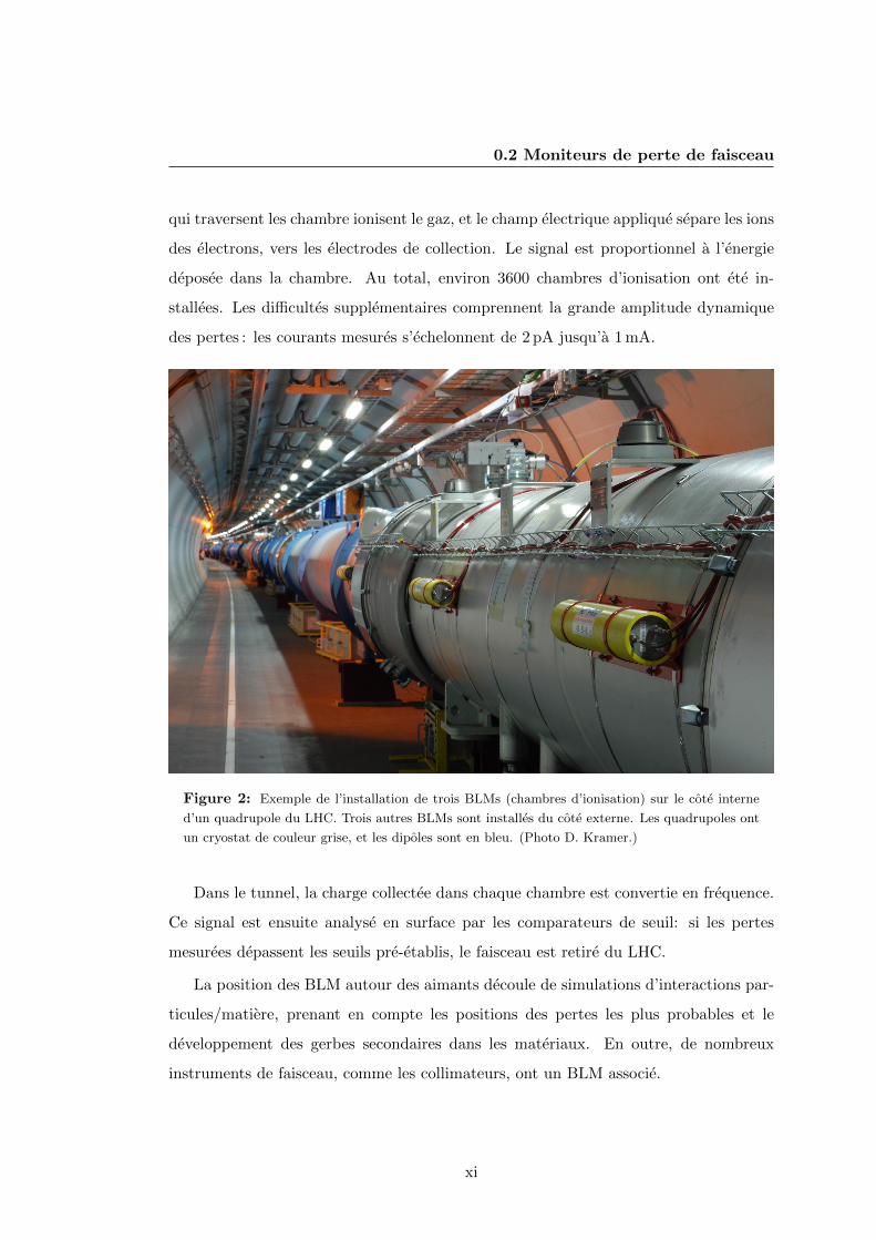
Figure 2: Exemple de l’installation de trois BLMs (chambres d’ionisation) sur le cote interne
d’un quadrupole du LHC. Trois autres BLMs sont installes du cote externe. Les quadrupoles ont
un cryostat de couleur grise, et les dipoles sont en bleu. (Photo D. Kramer.)
Dans le tunnel, la charge collectee dans chaque chambre est convertie en frequence.
Ce signal est ensuite analyse en surface par les comparateurs de seuil: si les pertes
mesurees depassent les seuils pre-etablis, le faisceau est retire du LHC.
La position des BLM autour des aimants decoule de simulations d’interactions par-
ticules/matiere, prenant en compte les positions des pertes les plus probables et le
developpement des gerbes secondaires dans les materiaux. En outre, de nombreux
instruments de faisceau, comme les collimateurs, ont un BLM associe.
xi

0.3 Interet du travail doctoral
Avant le debut de ce travail doctoral, de nombreuses etudes des pertes avaient ete
effectuees a l’echelle locale: autour d’un element. Cependant, aucune eude n’avait ete
effectuee a l’echelle globale, en considerant tous les moniteurs du LHC en meme temps.
La seule information donnee par un moniteur est la mesure des pertes a l’element
associe; mais une seule gerbe secondaire peut etre detectee par plusieurs moniteurs;
et certains des effets a l’orgine de pertes impliquent tout le LHC. Le nombre eleve de
BLMs necessite un traitement automatique.
Le sujet de cette these est d’etudier les structures de pertes et de trouver l’origine
des pertes de facon deterministe, en comparant des profils de pertes mesures a des
scenarios de pertes connus. Ceci a ete effectue par le biais d’une etude de cas : differentes
techniques ont ete utilisees sur un ensemble restreint de scenarios de pertes, constituant
une preuve de concept de la possibilite d’extraire de l’information d’un profil de pertes.
Trouver l’origine des pertes doit pouvoir permettre d’agir en consequence, ce qui justifie
l’interet du travail doctoral.
Ce travail de these se focalise sur la comprehension de la theorie et la mise en
place de la decomposition d’un profil de pertes mesure en une combinaison lineaire des
scenarios de reference ; sur l’evaluation de l’erreur sur la recomposition et sa validite.
0.4 Principe de la decomposition vectorielle
0.4.1 Espace vectoriel
Un profil de pertes est un ensemble de pertes mesurees par differents moniteurs (situes
a differentes positions longitudinales le long du LHC) a un instant donne. On considere
d’abord m moniteurs, et un espace vectoriel de dimension m associe. Chaque profil de
pertes peut donc etre represente comme un vecteur de cet espace vectoriel, ou chaque
coordonnee j du vecteur est la perte mesuree au moniteur j. En outre, des pertes
negatives n’ont aucune realite physique: les coordonnees des vecteurs sont donc toutes
positives, et on ne considere que la partie positive de l’espace vectoriel : (R+)m. Les
vecteurs sont tous normalises pour avoir une norme de valeur 1.
On considere ensuite n profils de pertes de reference, et leurs vecteurs associes (~vi).
Il est important de noter que n < m. Enfin, on considere un profil de pertes mesure
xii

0.4 Principe de la decomposition vectorielle
appele ~X.
Le but de la decomposition vectorielle est de decomposer ~X en une combinaison
lineaire des vecteurs (~vi), c’est-a-dire de resoudre l’equation vectorielle:
~X = a · ~v1 + b · ~v2 + · · · pour les {a, b, . . .} (1)
Pour cela, deux techniques sont utilisees: par une succession de projections des
vecteurs (~vi) (non orthogonaux) dans l’espace vectoriel (procede de Gram-Schmidt, G-
S); et par des operations matricielles. Puisque n < m, la matrice des vecteurs (~vi) (notee
M) n’est pas carree, et son inversion n’est pas simple. On utilise donc l’algorithme de
decomposition en valeurs singulieres (Singular Values Decomposition, SVD).
x1
x2
x3
V1
V2
Base canonique
P: sous-espace généré par fV
1, V
2g
X
X'
e
V1, V
2: vecteurs de référence
X: vecteur mesuré (X2P)
X' : combinaison linéaire de V
1 et V
2
la plus proche de X (X'2P)
e = kX–X'k : ``erreur” sur la recomposition
Figure 3: Exemple simplifie de decomposition vectorielle en 3 dimensions: n = 2, m = 3. Le
vecteur ~X n’appartient pas au sous-espace P genere par ( ~V1, ~V2). La recomposition ~X ′ correspond
a la projection de ~X sur P . L’erreur sur la recomposition correspond a la norme euclidenne de la
difference entre ~X et ~X ′.
Il est important de noter que le vecteur ~X n’appartient pas forcement au sous-
espace genere par les vecteurs de reference (~vi) (cf. fig. 3). Pour evaluer la qualite
de la decomposition, une erreur sur la recomposition e a ete definie comme la norme
euclidienne du vecteur de la difference entre le vecteur mesure ~X et sa recomposition ~X ′.
xiii

∣∣∣∣∣∣∣∣∣∣
(~v1) · · · (~vn)∣∣∣∣∣∣∣∣∣∣
︸ ︷︷ ︸
Mm×n
=
∣∣∣∣∣∣∣∣∣∣
(~u1) · · · · · · (~um)∣∣∣∣∣∣∣∣∣∣
︸ ︷︷ ︸
Um×m
·
λ1 0 · · · 0
0 λ2 · · · 0...
.... . .
...
0 0 · · · λn
0 0 · · · 0...
......
0 0 · · · 0
︸ ︷︷ ︸
Σm×n
·
—(~w1)—
...
—(~wn)—
︸ ︷︷ ︸
WTn×n
Figure 4: Structure des matrices utilisees dans la decomposition. M est la matrice de
depart, composee des vecteurs (~vi); U et W sont les matrices des vecteurs singuliers a
droite et a gauche respectivement. Σ une matrice diagonale (ou n < m) contenant les
valeurs singulieres: toutes ses valeurs sont nulles sauf celles de la diagonale λi = (Σ)i,i.
0.4.2 Decomposition en Valeurs Singulieres (SVD)
L’equation vectorielle (1) peut s’ecrire sous forme matricielle:
~X = M · ~F (2)
ou ~F est le vecteur forme par les coefficients {a, b, . . . } et M est la matrice formee par
les vecteurs (~vi).
La matrice M n’etant pas carree, on utilise d’abord la decomposition en valeurs
singulieres (SVD, cf. fig. 4) pour pouvoir l’inverser ulterieurement:
M = U · Σ ·W
La matrice inverse M+ est calcule par:
M+ ≡W · Σ+ · UT
Le vecteur ~F est donne par:
~F 'M+ · ~X
et la recomposition ~X ′ par:
~X ′ = M · ~F ' M ·M+ · ~X
xiv

0.5 Mise en place de la decomposition vectorielle
v1
v2 { c
1!2
c1!2
v2
c1!2
Figure 5: Premiere etape du procede de Gram-Schmidt. On calcule la projection (en
noir) de ~v2 (en bleu) sur ~v1 (en rouge), ce qui correspond a la contribution de ~v1 a ~v2.
Puis on soustrait cette contribution pour obtenir un vecteur perpendiculaire a ~v1 (en vert).
Cette operation est ensuite repetee avec le vecteur suivant.
0.4.3 Le procede de Gram-Schmidt (G-S)
Le procede de Gram-Schmidt (G-S) est un ensemble d’operations vectorielles visant
a creer une base orthonormale a partir d’un ensemble de vecteurs non orthogonaux
(cf. fig. 5). Une fois une base orthonormale creee, le vecteur ~X peut etre projete.
Cependant, la base n’est pas unique: elle depend de l’ordre dans lequel les vecteurs
(~vi) sont consideres. Les vecteurs sont donc ordonnes suivant leur distance (norme
euclidenne de la difference) a ~X.
0.5 Mise en place de la decomposition vectorielle
Un ensemble de scenarios de pertes connus ont ete reunis, permettant l’etude et la
creation de vecteurs de reference. Ces scenarios correspondent a l’augmentation de la
taille du faisceau dans les plans vertical et horizontal lors du passage de la resonnance
1/3 du tune du LHC, et a la difference d’energie (plan longitudinal) lors de mesures de
profils de pertes, pour chaque faisceau. Ces six scenarios correspondent aux collimateurs
primaires du LHC.
L’ensemble des moniteurs significatifs (representant les coordonnees des vecteurs)
a ete choisi suivant des regles specifiques. Ces moniteurs devaient:
� presenter un ecart–type tres faible (negligeable devant la valeur moyenne) calcule
xv

Figure 6: Exemple de selection des profils de pertes apres normalisation, pour les moniteurs du
point 7, et le scenario correspondant au faisceau 2 horizontal. Les etoiles bleues correspondent a la
valeur de l’ecart–type normalise pour les moniteurs selectionnes. La qualite de la reproductibilite
des mesures est visible par le fait que les profils sont presque indiscernables apres normalisation;
et par les valeurs d’ecart-type, autour de 1% de la valeur moyenne pour chaque moniteur.
sur l’ensemble des mesures correspondant a un seul scenario (afin de s’assurer que
le moniteur soit bien representatif);
� presenter un ecart–type important lorsque calcule pour les mesures des tous les
scenarios possibles (afin de s’assurer que le moniteur soit bien discriminant d’un
scenario a un autre).
La selection finale des moniteurs pour le point 7 (plans transverses) est presentee dans
la table 4.2. Pour le plan longitudinal, la meme technique de selection a ete utilisee,
mais aucun profil de pertes n’est disponible pour un faisceau isole car les deux faisceaux
sont acceleres en meme temps. Des profils de pertes on pu etre recrees en assignant
une valeur nulle aux moniteurs associes au faisceau non considere. Les collimateurs
tertiaires ont aussi ete ajoutes, en leur associant le vecteur canonique correspondant,
puisqu’aucun profil de perte n’est disponible.
Enfin, puisque la decomposition donne toujours un resultat, la justesse de la decomposition
doit etre evaluee, en utilisant l’erreur sur la recomposition (cf. fig. 3). La decomposition
xvi

0.6 Evolution temporelle
de profils de pertes connus correspondand a des scenarios connus permet de juger si
le resultat de la decomposition est correct ou non. Les differents resultats ont permis
d’etablir des seuils dans la valeur de l’erreur: en-dessous de 0.1, la decomposition est
correcte; au-dessus de 0.3, elle est incorrecte.
0.6 Evolution temporelle
Les outils de decomposition vectorielle ont ete systematiquement utilises pour etudier
l’evolution temporelle des pertes. D’abord, la variation d’une seconde a l’autre du profil
de perte contenant les 3600 moniteurs du LHC a ete considere, puis differentes compara-
isons avec un profil de pertes par defaut calcule pour l’occasion. Ceci a montre que les
differentes quantites considerees etait bien equivalentes, mais que la plus representative
etait bien la norme de la difference avec un vecteur fixe, comme pour l’erreur sur la
recomposition.
Figure 7: Profil de pertes par defaut, represente par un histogramme a 2 dimensions, mesure
pendant ' 70 h. Chaque colonne correspond a un moniteur: l’indice du moniteur est indique sur
l’axe horizontal, et la valeur de la perte a chaque seconde est reportee sur l’axe vertical. Le nombre
d’entrees par case (pertes de meme intensite) est represente par l’echelle de couleurs. Les 8 arcs
sont visibles, separes par les regions d’insertion (pertes plus elevees).
Le profil de pertes par defaut, mesure sur une centaine d’heures de faisceaux stable,
xvii

a apporte de nombreuses observations. Durant la periode consideree, aucune perte
n’a ete enregistree dans les arcs, et la resolution de la mesure est inferieur a un bit
du systeme d’acquisition. Les seuls moniteurs pertinents pour cette etude sont ceux
qui presentent une fluctuation importante, justifiant le choix des points 3 et 7, et des
collimateurs tertiaires.
0.7 Decomposition spatiale
Les resultats des decompositions ont ete calcules pour les pertes a chaque seconde des
periodes de “faisceaux stables” de l’annee 2011, pour l’etude de la distribution spatiale
des pertes. Les facteurs sont presente en fonction du temps, pour les deux techniques de
decomposition; l’erreur sur la recomposition est aussi representee sur le meme graphe
(cf. fig. 8). Les facteurs associes au collimateurs tertiaires sont representes sur un
graphe a part. Ceci permet de visualiser quel type de pertes domine le vecteur mesure
a chaque seconde.
Figure 8: Exemple de representation des resultats de la decomposition (SVD) en fonction du
temps. La decomposition est dominee par le facteur du faisceau 2 horizontal. L’erreur sur la
recomposition est representee en rouge. Les pertes associees au plan longitudinal augmentent au
cours des trois premieres heures, puis se stabilisent (autour de 10 000 secondes).
Les resultats obtenus ont ete compares avec les mesures d’autres instruments de fais-
xviii

0.8 Conclusion & Appendices
ceau, pour permettre differentes validations. Une premiere validation a ete de verifier
que les pertes de faisceau se comportent bien comme la derivee de l’intensite dans ce
faisceau, lors d’une periode de faisceau stable ou l’intensite diminuait plus rapidement
dans le faisceau 1 que dans le faisceau 2.
La validite de la decomposition a aussi ete verifiee lors d’operations sur les faisceaux
pendant lesquels differents collimateurs sont refermes, creant des pertes importantes.
Meme lorsque deux collimateurs etaient deplaces en meme temps, la decomposition
est clairement dominee par un seul facteur; ceci est verifie par les intensites dans les
faisceaux, qui ne varient pas en meme temps.
0.8 Conclusion & Appendices
En conclusion, l’interet de la decomposition vectorielle est presente. Des structures
spatiales de pertes ont ete identifiees, et des techniques ont ete developpees pour per-
mettre de les identifier dans un profil de pertes mesure. La justesse de la decomposition
a ete evaluee, et les resultats verifie grace a d’autres instruments de mesure du faisceau.
Un profil de pertes par defaut a aussi ete mesure pour etudier l’evolution temporelle
des pertes.
L’outil de decomposition a depuis ete adapte pour etre utilise en temps reel dans
le centre de controle du LHC, et aider a l’operation de la machine et detecter des
pertes inhabituelles. La validite des resultats depend des vecteurs de reference. Les
possibilites d’utilisation pourraient etre etendue en creant de nouveaux vecteurs, pour
d’autres scenarios, d’autres modes de faisceau; ou meme en utilisant d’autres techniques
de decomposition. L’outil pourrait meme etre utilise dans d’autres machines ou des
profils de pertes peuvent etre mesures.
En appendice est decrit le code developpe pour permettre l’acces aux donnees des
BLMs, pour les representer de facon utilisable, et pour les enregistrer. Ceci inclus la
connexion a differentes bases de donnees. L’instrument utilise des objets ROOT pour
envoyer des requetes SQL aux bases de donnees ainsi que par une interface Java, et est
code en Python.
Un court glossaire des acronymes utilises dans cette these est disponible a la fin du
document, avant la bibliographie.
xix

xx

Contents
Acknowledgements ii
Summary v
Resume vii
Synthese ix
0.1 La protection du LHC . . . . . . . . . . . . . . . . . . . . . . . . . . . . ix
0.2 Moniteurs de perte de faisceau . . . . . . . . . . . . . . . . . . . . . . . x
0.3 Interet du travail doctoral . . . . . . . . . . . . . . . . . . . . . . . . . . xii
0.4 Principe de la decomposition vectorielle . . . . . . . . . . . . . . . . . . xii
0.4.1 Espace vectoriel . . . . . . . . . . . . . . . . . . . . . . . . . . . xii
0.4.2 Decomposition en Valeurs Singulieres (SVD) . . . . . . . . . . . xiv
0.4.3 Le procede de Gram-Schmidt (G-S) . . . . . . . . . . . . . . . . xv
0.5 Mise en place de la decomposition vectorielle . . . . . . . . . . . . . . . xv
0.6 Evolution temporelle . . . . . . . . . . . . . . . . . . . . . . . . . . . . . xvii
0.7 Decomposition spatiale . . . . . . . . . . . . . . . . . . . . . . . . . . . . xviii
0.8 Conclusion & Appendices . . . . . . . . . . . . . . . . . . . . . . . . . . xix
1 LHC protection 1
1.1 CERN . . . . . . . . . . . . . . . . . . . . . . . . . . . . . . . . . . . . . 1
1.2 The Large Hadron Collider . . . . . . . . . . . . . . . . . . . . . . . . . 3
1.2.1 Characteristics . . . . . . . . . . . . . . . . . . . . . . . . . . . . 3
1.2.2 Experiments . . . . . . . . . . . . . . . . . . . . . . . . . . . . . 4
1.2.3 Chain of previous accelerators . . . . . . . . . . . . . . . . . . . . 7
1.2.4 Beam optics & acceleration . . . . . . . . . . . . . . . . . . . . . 8
xxi

CONTENTS
1.2.5 Beam modes . . . . . . . . . . . . . . . . . . . . . . . . . . . . . 8
1.3 Magnets . . . . . . . . . . . . . . . . . . . . . . . . . . . . . . . . . . . . 9
1.4 Collimators . . . . . . . . . . . . . . . . . . . . . . . . . . . . . . . . . . 10
1.4.1 Machine Protection . . . . . . . . . . . . . . . . . . . . . . . . . 11
1.4.2 Collimation . . . . . . . . . . . . . . . . . . . . . . . . . . . . . . 12
1.4.3 Types of collimators . . . . . . . . . . . . . . . . . . . . . . . . . 13
1.4.4 Performances & requirements . . . . . . . . . . . . . . . . . . . . 15
1.4.5 Beam measurements involving collimators . . . . . . . . . . . . . 16
1.5 Conclusion . . . . . . . . . . . . . . . . . . . . . . . . . . . . . . . . . . 19
2 The BLM System 21
2.1 The monitors . . . . . . . . . . . . . . . . . . . . . . . . . . . . . . . . . 21
2.1.1 Ionisation Chambers . . . . . . . . . . . . . . . . . . . . . . . . . 21
2.1.2 Installation . . . . . . . . . . . . . . . . . . . . . . . . . . . . . . 22
2.2 Time Structure: Running Sums . . . . . . . . . . . . . . . . . . . . . . . 23
2.3 Electronics . . . . . . . . . . . . . . . . . . . . . . . . . . . . . . . . . . 25
2.3.1 In the tunnel . . . . . . . . . . . . . . . . . . . . . . . . . . . . . 26
2.3.2 On the surface . . . . . . . . . . . . . . . . . . . . . . . . . . . . 29
2.4 Thresholds . . . . . . . . . . . . . . . . . . . . . . . . . . . . . . . . . . 29
2.5 Justification of the doctoral work . . . . . . . . . . . . . . . . . . . . . . 31
3 Principle of Vector Decomposition 33
3.1 Principle . . . . . . . . . . . . . . . . . . . . . . . . . . . . . . . . . . . . 33
3.1.1 Motivation . . . . . . . . . . . . . . . . . . . . . . . . . . . . . . 33
3.1.2 Vector space . . . . . . . . . . . . . . . . . . . . . . . . . . . . . 33
3.1.3 Vector decomposition . . . . . . . . . . . . . . . . . . . . . . . . 34
3.1.4 Projections . . . . . . . . . . . . . . . . . . . . . . . . . . . . . . 35
3.1.5 Matrix inversion . . . . . . . . . . . . . . . . . . . . . . . . . . . 35
3.2 Singular Value Decomposition (SVD) . . . . . . . . . . . . . . . . . . . . 36
3.2.1 Principle . . . . . . . . . . . . . . . . . . . . . . . . . . . . . . . 36
3.2.2 Advantages . . . . . . . . . . . . . . . . . . . . . . . . . . . . . . 37
3.2.3 Important observations . . . . . . . . . . . . . . . . . . . . . . . 38
3.2.4 Pseudoinverse . . . . . . . . . . . . . . . . . . . . . . . . . . . . . 39
3.2.5 Recomposition . . . . . . . . . . . . . . . . . . . . . . . . . . . . 39
xxii
CONTENTS
3.2.6 Limitations . . . . . . . . . . . . . . . . . . . . . . . . . . . . . . 40
3.3 Gram-Schmidt process . . . . . . . . . . . . . . . . . . . . . . . . . . . . 41
3.3.1 Technique . . . . . . . . . . . . . . . . . . . . . . . . . . . . . . . 41
3.3.2 Importance of the order of the vectors . . . . . . . . . . . . . . . 42
3.4 MICADO . . . . . . . . . . . . . . . . . . . . . . . . . . . . . . . . . . . 43
3.5 Recomposition and error . . . . . . . . . . . . . . . . . . . . . . . . . . . 44
3.5.1 Motivation . . . . . . . . . . . . . . . . . . . . . . . . . . . . . . 44
3.5.2 Evaluation of the error . . . . . . . . . . . . . . . . . . . . . . . . 44
3.6 Conclusion . . . . . . . . . . . . . . . . . . . . . . . . . . . . . . . . . . 46
4 Implementation of Vector Decomposition 47
4.1 Creation of the default vectors . . . . . . . . . . . . . . . . . . . . . . . 47
4.1.1 Choice of beam loss scenarios . . . . . . . . . . . . . . . . . . . . 47
4.1.2 Dates of measurement . . . . . . . . . . . . . . . . . . . . . . . . 49
4.1.3 Normalisation . . . . . . . . . . . . . . . . . . . . . . . . . . . . . 51
4.1.4 Effect of the BLM offset . . . . . . . . . . . . . . . . . . . . . . . 51
4.2 Choice of the list of BLMs . . . . . . . . . . . . . . . . . . . . . . . . . . 53
4.2.1 Problem . . . . . . . . . . . . . . . . . . . . . . . . . . . . . . . . 53
4.2.2 Selection technique . . . . . . . . . . . . . . . . . . . . . . . . . . 55
4.3 Final loss map selection . . . . . . . . . . . . . . . . . . . . . . . . . . . 57
4.3.1 Dependency on energy . . . . . . . . . . . . . . . . . . . . . . . . 57
4.3.2 Order of the loss maps . . . . . . . . . . . . . . . . . . . . . . . . 60
4.3.3 Reproducibility for IR7 . . . . . . . . . . . . . . . . . . . . . . . 60
4.4 Adding more cases: longitudinal scenarios and TCTs . . . . . . . . . . . 60
4.4.1 Longitudinal loss maps . . . . . . . . . . . . . . . . . . . . . . . . 61
4.4.2 Intensity derivative . . . . . . . . . . . . . . . . . . . . . . . . . . 62
4.4.3 Choice of the monitors . . . . . . . . . . . . . . . . . . . . . . . . 63
4.4.4 Creation of the longitudinal vectors . . . . . . . . . . . . . . . . 64
4.4.5 Tertiary collimators . . . . . . . . . . . . . . . . . . . . . . . . . 65
4.4.6 Final loss maps — reproducibility . . . . . . . . . . . . . . . . . 66
4.5 Validation of results: Centers of Mass . . . . . . . . . . . . . . . . . . . 73
4.5.1 Motivation . . . . . . . . . . . . . . . . . . . . . . . . . . . . . . 73
4.5.2 Implementation and verifications . . . . . . . . . . . . . . . . . . 74
xxiii

CONTENTS
4.6 Choice of the algorithm . . . . . . . . . . . . . . . . . . . . . . . . . . . 78
4.7 Evaluation of the correctness of a decomposition . . . . . . . . . . . . . 79
4.7.1 Correct and incorrect decompositions . . . . . . . . . . . . . . . 79
4.7.2 Method and results . . . . . . . . . . . . . . . . . . . . . . . . . . 79
4.7.3 Distributions of the error for the 2011 loss maps . . . . . . . . . 81
4.7.4 Conclusion on the values of the error . . . . . . . . . . . . . . . . 83
4.8 Application to LHC data . . . . . . . . . . . . . . . . . . . . . . . . . . 83
4.8.1 Implementation . . . . . . . . . . . . . . . . . . . . . . . . . . . . 83
4.8.2 Evolution of losses . . . . . . . . . . . . . . . . . . . . . . . . . . 84
4.8.3 Default Loss Profile . . . . . . . . . . . . . . . . . . . . . . . . . 89
5 Time evolution 91
5.1 Default Loss Profile . . . . . . . . . . . . . . . . . . . . . . . . . . . . . 91
5.1.1 Interest . . . . . . . . . . . . . . . . . . . . . . . . . . . . . . . . 91
5.1.2 Creation . . . . . . . . . . . . . . . . . . . . . . . . . . . . . . . . 93
5.1.3 Observations . . . . . . . . . . . . . . . . . . . . . . . . . . . . . 93
5.1.4 Comparisons with default loss profile . . . . . . . . . . . . . . . . 94
5.2 Individual evolution of the signal of a BLM . . . . . . . . . . . . . . . . 96
5.2.1 Arc monitor — low signal . . . . . . . . . . . . . . . . . . . . . . 96
5.2.2 Variations of the signal of a monitor . . . . . . . . . . . . . . . . 98
5.2.3 IP monitors — high signal . . . . . . . . . . . . . . . . . . . . . . 99
5.3 Evolution of the overall losses . . . . . . . . . . . . . . . . . . . . . . . . 102
5.4 Conclusion . . . . . . . . . . . . . . . . . . . . . . . . . . . . . . . . . . 104
6 Spatial decomposition 105
6.1 Results of decomposition . . . . . . . . . . . . . . . . . . . . . . . . . . . 105
6.1.1 Presentation of the results . . . . . . . . . . . . . . . . . . . . . . 105
6.1.2 Displaying the decomposition . . . . . . . . . . . . . . . . . . . . 106
6.2 Examples of decomposition versus time . . . . . . . . . . . . . . . . . . 107
6.2.1 Error propagation for the factors . . . . . . . . . . . . . . . . . . 108
6.3 Validation of results . . . . . . . . . . . . . . . . . . . . . . . . . . . . . 114
6.3.1 Beam intensities . . . . . . . . . . . . . . . . . . . . . . . . . . . 114
6.3.2 Correlation with the result of the decomposition . . . . . . . . . 121
6.3.3 Collimator scraping . . . . . . . . . . . . . . . . . . . . . . . . . 124
xxiv
CONTENTS
6.4 Conclusion . . . . . . . . . . . . . . . . . . . . . . . . . . . . . . . . . . 126
Global conclusion 127
Appendix 129
A Data Access 129
A.1 Introduction . . . . . . . . . . . . . . . . . . . . . . . . . . . . . . . . . . 129
A.1.1 Beam losses . . . . . . . . . . . . . . . . . . . . . . . . . . . . . . 129
A.1.2 Introduction to the Beam Loss Analysis Toolbox . . . . . . . . . 129
A.2 Data & databases . . . . . . . . . . . . . . . . . . . . . . . . . . . . . . . 131
A.2.1 Data structure . . . . . . . . . . . . . . . . . . . . . . . . . . . . 131
A.2.2 Layout database . . . . . . . . . . . . . . . . . . . . . . . . . . . 132
A.2.3 Measurement database and Logging database . . . . . . . . . . . 132
A.3 Database Access Techniques . . . . . . . . . . . . . . . . . . . . . . . . . 133
A.3.1 PL/SQL Access . . . . . . . . . . . . . . . . . . . . . . . . . . . . 133
A.3.2 Java access . . . . . . . . . . . . . . . . . . . . . . . . . . . . . . 136
A.3.3 Structure of the returned object . . . . . . . . . . . . . . . . . . 138
A.4 Display . . . . . . . . . . . . . . . . . . . . . . . . . . . . . . . . . . . . 140
A.4.1 Plotting with ROOT . . . . . . . . . . . . . . . . . . . . . . . . . 141
A.4.2 Signal vs. time . . . . . . . . . . . . . . . . . . . . . . . . . . . . 141
A.4.3 Plotting the LHC . . . . . . . . . . . . . . . . . . . . . . . . . . . 143
A.4.4 XY plots . . . . . . . . . . . . . . . . . . . . . . . . . . . . . . . 145
A.4.5 Plotting Running Sums . . . . . . . . . . . . . . . . . . . . . . . 146
A.4.6 Methods shared by all plots . . . . . . . . . . . . . . . . . . . . . 147
A.5 The wrapping module: analysis . . . . . . . . . . . . . . . . . . . . . . . 147
A.5.1 Basic behaviour . . . . . . . . . . . . . . . . . . . . . . . . . . . . 148
A.5.2 Process . . . . . . . . . . . . . . . . . . . . . . . . . . . . . . . . 150
A.5.3 Advanced functionalities . . . . . . . . . . . . . . . . . . . . . . . 153
A.6 Conclusion . . . . . . . . . . . . . . . . . . . . . . . . . . . . . . . . . . 162
B Cross-checks 163
Glossary 167
Bibliography 169
xxv

CONTENTS
xxvi

Chapter 1
The Large Hadron Collider and
its protection
1.1 CERN
When CERN was founded in 1954, the name originally meant “Conseil Europeen pour la
Recherche Nucleaire”, referring to a provisional body founded two years earlier. Its goal
was to establish a world-class fundamental physics research organization in Europe. At
the time, the most fundamental physics research was the study of the inside of an atom,
thus the use of “nuclear” in the title of the new organisation: “European organisation
for nuclear research”. The name CERN was kept.
Today, the most fundamental physics studies concentrate on the basic constituents
of matter: the fundamental particles. This is done by increasing the energy of particles
in accelerators, and having the particles collide in detectors analysing these events.
CERN’s title is now the European laboratory for particle physics.
CERN is now the world’s largest laboratory. It is run by 20 countries: Germany,
France, United Kingdom, Italy, Spain, the Netherlands, Switzerland, Poland, Belgium,
Sweden, Norway, Austria, Greece, Denmark, Finland, the Czech Republic, Portugal,
Hungary, Slovakia, and Bulgaria. Many other countries, including Russia, Japan and
the United States, are involved in the CERN programs.
The mission of CERN is clearly described in its convention:
“The Organization shall provide for collaboration among European States in nuclear
research of a pure scientific and fundamental character (...). The Organization shall
1

1. LHC PROTECTION
Figure 1.1: The chain of accelerators at CERN, from the linear accelerators to the detectors of
the LHC, including all other CERN experiments and the different types of particles. LHC protons
start at Linac 2, then are transfered successively into the Booster, the PS, the SPS and finally the
LHC. The North Area is an extraction on fixed targets for mixed radiation field tests.
have no concern with work for military requirements and the results of its experimental
and theoretical work shall be published or otherwise made generally available”.
Around 3000 people are employed by CERN; in addition, another 6500 scientists
from 500 universities and 80 countries work with CERN equipments or directly at
CERN.
CERN’s biggest and most famous accelerator is the Large Hadron Collider (LHC),
which hosts four main experiments: ALICE, ATLAS, CMS and LHCb. Each of them
is the product of the collaboration of several thousands of people and a wide range
of experimental facilities. CERN also operates many other different accelerators and
experiments (cf. fig. 1.1); however, these other experiments will not be described,
2

1.2 The Large Hadron Collider
Circumference 26 659 m
Number of magnets 9593
Number of main dipoles 1232
Dipole operating temperature 1.9 K
Peak magnetic dipole field 8.33 T
Number of main quadrupoles 392
Number of RF cavities 8 per beam
Nominal energy, protons 7 TeV
Nominal energy per nucleon, ions 2.76 TeV
Design luminosity 1034 cm−2 · s−1
No. of bunches per proton beam 2808
No. of particles per bunch 1.15 · 1011 p
Nominal intensity 3.2 · 1014 p
Revolution frequency 11 245 Hz
Revolution period 88.924 µs
Min. bunch spacing 25 ns
Collision rate 600 MHz
Energy stored per beam (at 7 TeV) 362 MJ
Energy stored in the magnets (at 7 TeV) 10 GJ
Table 1.1: Nominal values of the main characteristics of the LHC, from (1), (9).
because they are not part of the scope of this work.
1.2 The Large Hadron Collider
1.2.1 Characteristics
The LHC is the largest machine ever built, with a total circumference of 26.7 km.
Today, it is the biggest accelerator, but also the one with the highest energy, intensity
and luminosity. Some of the most important characteristics of the LHC are given in
tab. 1.1.
The role of the LHC is to increase the energy of the two counter-circulating beams
of injected protons, and to make them collide in the four interactions points where the
four experiments are installed. During a collision, the enormous amounts of energy lead
to the creation of many other particle through the famous equivalence between mass
3

1. LHC PROTECTION
and energy. These newly created particles — and their decay products if they are not
stable — can be detected by the experiments. The LHC can also accelerate lead ions
nuclei.
The LHC itself is divided in eight straight insertion regions (IR), separated by eight
bending sections called arcs which form most of the LHC (cf. fig. 1.2). In the arcs,
the beams are simply transported. Each arc is made of 46 regular cells, which are
composed of three 14.3 m dipole magnets and one 3.1 m quadrupole magnet. The cells
are numbered from the middle of the IR towards the middle of the arc, left or right
of the IR seen from the center of the ring. All interaction regions are also commonly
referred to as “interaction points” (IP). Collisions only happen at the interaction points
holding the experiments: ATLAS in IR1, ALICE in IR2, CMS in IR5 and LHCb in
IR8. IR3 and 7 are dedicated to the cleaning of the beam; the acceleration by the
radio-frequency chambers is done in IR4; and the extraction lines towards the beam
absorber are situated in IR6.
Given the perimeter of the LHC and the corresponding frequency (for particles
going at the speed of light), the space between bunches and the average number of
collisions per bunch crossing, approximately 600 million collisions take place during
one second. One of the challenges of the experiments was to have the processing power
to deal with such an immense amount of information.
1.2.2 Experiments
Four of the 8 insertion regions of the LHC are dedicated to four big experiments: CMS,
ATLAS, ALICE and LHCb.
CMS
The Compact Muon Solenoid (CMS), installed in IR5, is one of the two general-purpose
experiments of the LHC. It has the standard structure of the previous general-purpose
particle detectors in other accelerators. First (from the interaction point outwards) a
silicon tracker, made of several layers of pixels, tracks the particle trajectories, giving
their charge and momentum. Then, a homogeneous electromagnetic calorimeter mea-
sures the energy of particles sensitive to electromagnetic interactions, such as electrons
and photons, by stopping them entirely. All their energy is deposited in the very dense
4

1.2 The Large Hadron Collider
Figure 1.2: Schematics of the layout of the LHC, with the purpose of the different insertion
regions. Beam 1 is represented in blue and goes clockwise, beam 2 is in red and goes anticlockwise.
The collisions take place where the light blue stars are. The IRs are number clockwise starting at
Atlas (IR1).
5

1. LHC PROTECTION
lead tungstate crystals. The next layer is a hadronic calorimeter, made of dense ma-
terial such as brass and steel and plastic scintillators reading the signals. It is also
homogeneous to try and deposit as much energy as possible before the next layer: the
toroidal magnet.
In order to measure the charge and momentum of the created particles, their tra-
jectories are bent by a magnetic field: these values are calculated from the curvature
radius. The magnetic field of 3.8 T must be as uniform as possible, and is generated
by a 6 m wide, 13 m long superconducting toroidal magnet. Outside the magnets are
detectors dedicated to the only particles that can escape the calorimeters because of
their higher mass: the muons. In total, CMS is 15 m wide, 21.5 m long and weights
12 550 t.
ATLAS
ATLAS, standing for “A Toroidal Lhc ApparatuS”, is another general-purpose detec-
tor, installed in IR1. It has three trackers: the pixel detector, the semi-conductor
tracker and the transition radiation tracker (made of drift tubes). The two calorime-
ters, electromagnetic and hadronic, are sampling calorimeters. They are made of two
different-purpose materials: one creates the particle shower (lead and stainless steel for
the electromagnetic calorimeter, steel for the hadronic one), the other measures the
deposited energy (liquid argon and scintillating tiles respectively). In both cases, the
total shower energy has to be estimated.
ATLAS has two magnets: an inner solenoid, situated around the inner trackers,
creates a field of 2 T. The eight outer barrel toroid magnets are 20 m long, store 1.6 GJ of
energy. These, as well as the end-cap toroidal magnet and their gear-shaped cryostats,
give ATLAS’ typical octagon shape. At the same location is the muon spectrometer
installed, which is similar to the inner trackers, only not as precise but bigger. ATLAS
is 46 m long, 25 m wide and weighs 7000 t.
ALICE
“A Large Ion Collider Experiment” (ALICE) is the LHC experiment dedicated to ion
collisions, installed in IR2. One of the main goals of these collisions is to create a
new state of matter called “quark-gluon plasma”, at an equivalent temperature of ten
6

1.2 The Large Hadron Collider
trillion degrees. This is thought to be the state of the universe during its first hundred
microseconds.
The structure of ALICE is more complicated than the ones of the other experi-
ments. It is made of nine sub-detectors, from tracking to time of flight and transitions
measurements. Measurements in ALICE require ion beams in the LHC instead of pro-
tons. The top energy per nucleus is 2.76 TeV, which corresponds to 575 TeV per ion,
and 1.15 PeV in the center of mass.
LHCb
LHCb, installed in IR8, is entirely asymmetric. It only measures particles created in a
cone around the beam pipe on one side of the interaction point. The “b” in the name,
standing for the b quark (beauty or bottom, the 3rd generation quark with a charge of
−1/3 e), gives the goal of this experiment: to study particles containing a b quark,
called b-hadrons. These particles are predominantly created close to the beam pipe.
The point of these studies is to understand the predominance of matter over an-
timatter in the universe, which corresponds to a violation of the CP symmetry. Like
other particle detectors, LHCb has trackers, electromagnetic and hadronic calorimeters,
muon detectors and a magnet. It also has Cherenkov detectors, and a vertex detector
which is one of the instrument getting the closest to the beam in the LHC, and can
move away for protection reasons.
1.2.3 Chain of previous accelerators
The LHC does not accelerate the protons to their maximum energy alone: it is at the
end of a chain of accelerators (cf. fig. 1.1). The protons originally come from a bottle
of hydrogen. The electrons are removed, leaving single charged protons. They are
accelerated to a kinetic energy of 50 MeV by the linear accelerator called LINAC2, and
injected into the Booster. The Booster is a synchrotron made of four superimposed
rings which have a circumference of 78 m. The protons are accelerated to 1.4 GeV, and
then injected into the Proton Synchrotron (PS), which has a circumference of 628.3 m.
The energy of the protons is increased up to 26 GeV, and the 50 ns bunch structure
is created. The protons are then injected into the Super Proton Synchrotron (SPS),
which has a circumference of 6.9 km, and they are accelerated to 450 GeV, before being
extracted to the LHC.
7

1. LHC PROTECTION
1.2.4 Beam optics & acceleration
The equipment used to accelerate particles are the Radio Frequency (RF) cavities.
They provide an oscillating electric field that will accelerate the particles when they
pass through the cavities, without disturbing them before and after the cavity (as a
fixed field would). The radio frequency also creates the bunch structure of the beams
and regulates the momentum. The particles circulate, passing through the RF many
times, allowing a progressive acceleration.
The trajectory of the particles is bend in a circle by a vertical magnetic field constant
with respect to the particle position, provided by dipoles called Main Bending (MB)
magnets. However, this is not enough to keep the particles on a stable orbit. Elements
which can focus the particle beam are needed: they are called Main Quadrupoles (MQ).
They generate a magnetic field whose strength along one axis of transversal plane
depends on the displacement of the particle on this axis: the further from the center
the particle, the stronger the field.
The quadrupoles will then focus the particles in one direction, and defocus in the
other. Particles with the highest displacement will experience the strongest field, which
will inflect their trajectory and direct the particle back towards the center. In the arcs,
only considering particle transportation, not beam instruments, the quadrupoles are
the places where particles have the highest displacement, i.e. are closest to the beam
pipe, and most likely to be lost. A succession of focusing and defocusing magnets (for
one axis; successively defocusing and focusing for the other), separated by bending
magnets, is needed to keep the particles going in a circle.
The envelop of all particle trajectories (i.e. the most outside ones) is called the
Beta function. Other higher-order effects such as variations in momentum and periodic
errors require higher orders magnets to insure a proper particle behaviour, such as
sextupoles compensating for chromaticity.
1.2.5 Beam modes
The LHC has two particle beams circulating in opposite directions and behaving inde-
pendently. Before producing physics data, the LHC goes through a series of preparation
phases to bring the beams into collision. These phases are called beam modes (3).
8

1.3 Magnets
The first step of a LHC run is the injection of a pilot bunch whose intensity is not
dangerous for the machine, at injection energy: 450 GeV. Then, during the injection
mode, more bunches are injected from the SPS into the LHC according to the current
filling pattern. Once all required bunches have been injected, the ramp is started. In
this phase, the protons are accelerated up to the collision energy (3.5 TeV at the time
of writing). The current in the magnets is increased accordingly: protons with higher
energy need a higher magnetic field to keep the same curvature radius, which is fixed
(beam pipe).
Once the nominal energy is reached (flat top), the squeeze mode can start. The
point is to decrease the value of the β function at the interaction points, bringing the
circulating particle into the smallest possible area to maximise the number of collisions.
The value is denoted βb, and this is achieved by the magnet triplets situated on each
side of the interaction points.
Once the beams have been brought into collision (during the adjust mode) and are
in collision, and the beam conditions (such as life time) are under control (3), the stable
beam mode is set. This mode makes up the most part of a physics run, and is the one
during which the physics data are taken.
1.3 Magnets
Part of the design of the LHC was imposed by the dimension of the pre-existing tunnel.
The tunnel was the one of the Large Electron-Positron collider, which was operated
between 1989 and 2000, then dismantled. The shape of the tunnel and the consequent
curvature radius, together with the energy goal of 7 TeV for the particles, imposed
strong requirements on the magnets. The value of the magnetic field needed for 7 TeV
protons is 8.3 T, which requires a current of 12 500 A.
The choice was made to use superconducting magnets. They are made of super-
conducting coils which can carry electric current with no resistance. There is no heat
dissipation, allowing to carry much greater currents for the same cable section, thus
producing higher magnetic field. Due to cooling issues in resistive coils, and the satu-
ration of iron yokes, the magnetic fields in non-superconducting magnets is limited to
about 2 T.
9

1. LHC PROTECTION
Figure 1.3: Geometry of the coils of the dipoles. The dipoles bend the proton trajectories in
the horizontal plane. The magnetic field lines, in red, are shared between the two beams.
The 12 500 A can be carried in titanium-nobium wires of a section of a few square
millimetres, instead of the 80 cm2 which would be needed for normally conducting cop-
per wires. Moreover, the current density in these copper wires would not be enough
to create the requested magnetic field. The magnetic saturation of the material would
prevent reaching such high fields. The absence of energy dissipation decreases the elec-
tric energy consumption, but increases the cost of cooling. The operating temperature
of the LHC magnets is 1.9 K. This is achieved by cooling down the magnets with liquid
helium.
The two beams of the LHC travel in separated beam pipes everywhere except at
the collision regions. The two beam pipes are in the same cryostat, 194 mm away from
each other. This is achieved by a two-in-one design. In a dipole, the four coils share
the same yoke and some field line: part of the field for one beam is used by the other
(cf. fig. 1.3). This design is a way to decrease the energy consumption of the LHC.
1.4 Collimators
In this section, the collimation system will be presented.
10

1.4 Collimators
1.4.1 Machine Protection
The energy of 362 MJ stored in each nominal beam of the LHC, at top energy of 7
TeV per beam, is unprecedented. It is enough to melt about 500 kg of copper, and
the maximum stored energy exceeds by a factor 1000 all other existing accelerators
(cf. fig. 1.4).
A deposited energy as little as 1 mJ/cm3, or a few-turns loss of a portion of the
beam as small as 3 · 10−9 of the nominal intensity of 3 · 1014 p (cf. tab. 1.1) is sufficient
to quench a superconducting magnet; a portion of 10−6 could damage the equipment
and lead to long downtimes (2).
0.01
0.1
1
10
100
1000
0.1 1 10 100 1000 10000
Sto
red b
eam
energ
y [M
J]
Beam momentum [GeV/c]
SNS
ISR
LEP2SppS
LHC (top)
LHC (inj)
SPSHERA
TEVATRON
Figure 1.4: Energy stored in the beam versus beam momentum for past and present accelerators,
from (5). The link between the two is the beam intensity. If the beam momentum is the most
“visible” value for fundamental research (some decay channels can only happen above a certain
energy), the machine protection challenges stand in the total energy stored in the beam.
Such losses must be avoided. The LHC is protected by active systems, which can
detect dangerous situations and consequently remove the beam permit from the Beam
Interlock System. This triggers a extraction of the beam from the machine towards an
absorber in a process called beam dump. Around 140 active system are connected to
the Beam Interlock System (4). Amongst the main ones are the Beam Loss Monitoring
11
1. LHC PROTECTION
(BLM) system and the Quench Protection System. The BLM system will be described
in chap. 2. The Quench Protection System measures the voltage in the superconducting
magnets, which should be zero for perfectly superconducting magnets (no resistance).
When the voltage drop across the magnets exceeds predefined thresholds, indicating
an increase in resistance coming from a starting resistive transition (quench), quench
heaters are triggered. They are thin resistive stripes, situated inside the superconduct-
ing coils. Their role is to heat the coil homogeneously so that the energy present in the
magnet is not dissipated in only one point of the coil. The electric current is safely ex-
tracted from the magnet in the meantime. If all the energy was lost at the same point,
the temperature increase would exceed the boiling temperature of helium, leading to
an increase of volume by a factor ' 750. The temperature increase can be enough to
melt the coil of the magnet.
Other systems, called passive, protect the LHC by providing dedicated places where
the protons can be lost safely, without any danger for the equipment. Passive protection
systems are collimators and absorbers installed in dedicated cleaning regions and in
front of sensitive equipment. They are aperture limitations: the parts of the LHC that
are the closest to the beam. When protons moves away from the nominal orbit, the
first component encountered should always be a collimator.
1.4.2 Collimation
In circular accelerators, particles undergo transverse oscillations around the central
orbit due to the successive focusing and defocusing, depending on their position and
angle. They are called betatron oscillations. Depending on their phase advance com-
pared to the accelerating radio-frequency cavities and their possible offset in energy or
momentum, the particles will similarly perform longitudinal oscillations.
The limit for the oscillations of the particles is the aperture of the beam pipe. Any
particle hitting material at an aperture limitation creates a secondary shower, and is
lost from the beam. The point of the collimation system is to provide places and pieces
of equipment on which the most external particles can be lost safely.
The collimators are robust beam elements designed to withstand the energy deposi-
tion of beam particles, while maximising dilution and absorption. Absorption depends
12

1.4 Collimators
Figure 1.5: Left: picture of one collimator jaw made of CFC (graphite). Right: The two
collimator jaws installed in the vacuum tank. The protons enter by the opening in the front of
the vacuum tank and move parallel to the jaw. The blue arrows represent the trajectories of the
particles. The collimator in the picture is horizontal.
on the inelastic interaction length of the material at the considered energies. Different
material and functionalities were chosen depending on the required functionalities.
The collimators are made of two jaws, controlling the beam size in one plane of the
beam optics (cf. fig. 1.5). The jaws are moved by step motors, which have a precision
of 5µm and are remotely controlled (5). The gap between the jaws can vary between
0.5 and 60 mm, depending on the optics at the collimator position and the beam mode.
It is often expressed in units of nominal σ, which is the standard deviation of the
transversal proton distribution, assumed to be Gaussian. It is a measure of the width
of the beam: σ =√β · ε, where ε is the emittance of the LHC, the value of the area
covered by the particles in the phase space. At injection, the typical value at the
primary collimator is σinj = 1 mm; at top energy, σtop = 0.3 mm.
1.4.3 Types of collimators
The collimation system is a multi-stage scattering and absorbing scheme, with different
types of collimators meeting different purposes (cf. fig. 1.6). In total, 132 collimator
locations have been reserved on the LHC. For the first phase of LHC operation, 88
collimators are installed and used. The main types of collimators are (5):
� Primary collimators (TCP). Their jaws are made out of graphite reinforced by
carbon fibers, called CFC. The goal of this low atomic number (Z) material is to
13

1. LHC PROTECTION
Pri
mary
Collim
ato
rBeam propagation
Sec
ondary
Col
lim
ato
r
Abso
rber
s
Ter
tiar
yC
ollim
ator
Beam Core
Secondary halo(disturbed protons)
p
p
Primary halo (p)
Tertiary halo (p)
Super-conducting & warm magnets
¼
¼
e
eshower Superconducting
magnets & particle physics
experiments
TCP TCSG TCLA TCT
Unavoidable losses
Hierarchy: respective retraction of the different types of collimators, further and further away from the beam.
Figure 1.6: Multi-stage cleaning scheme of the collimation system of the LHC. The acronyms
for the collimator names (TCT, TCSG, TCLS, TCT) are described in the text. The materials
are carbon fiber-reinforced graphite (CC), copper (CU) and tungsten (W). More details about the
installation of collimators are given in fig. 1.7.
scatter the protons from the beam halo: about 95% of the energy entering the
jaw leaves it again. The jaw length is 60 cm, and the nominal jaw opening (at
collisions at 7 TeV) for the transversal planes (IR7) is 6σ (6).
� Graphite Secondary Collimators (TCSG), also made of CFC. They intercept the
particle scattered by the primary collimators. Most of them are installed close to
the corresponding TCP. The jaw length is 100 cm, and the nominal jaw opening
(same conditions) is 7σ (6).
� Tertiary Collimators (TCT). They are made of tungsten, which has a high atomic
number, and are meant to protect the magnet triplets around the four experiments
in the LHC. The jaw length is 100 cm, and the nominal jaw opening is 8.3σ (6).
� Long absorbers (TCLA). They are made of tungsten or copper, and are meant to
stop the tertiary halo. They are installed at the end of the two cleaning regions,
14

1.4 Collimators
Figure 1.7: Installation of the collimators around the LHC (phase 1 of operation) (5). The red
names correspond to beam 1; the black ones to beam 2. In a collimator expert name, the letters
before the dot give the type of the collimator (cf. text); the letters after the dot give the position
of the collimator in the ring (including cell number). Most collimators for betatron cleaning are
installed around IP7; most collimators for momentum cleaning are installed around IP3.
to protect the superconducting elements of the arcs.The jaw length is 100 cm,
and the nominal jaw opening is 10σ (6).
Most collimators are installed in the two straight sections of the LHC that are
dedicated to collimation (cf. fig. 1.7): the Insertion Regions (IR) 3 and 7. IR3 holds
the collimators for momentum cleaning, including the two primary collimators (for
both beams). IR7 holds the collimators for betatron cleaning, including the 2 primary
collimators per beam for the horizontal and vertical planes (4 in total), as well as skew
collimators.
1.4.4 Performances & requirements
The performance of collimation in the LHC is quantified by the local cleaning ineffi-
ciency, which is the quantity of protons Ni lost at a location i of length Li, over the
total number of protons Ntot lost in the LHC :
ηcol ≡NiLi
Ntot(1.1)
15

1. LHC PROTECTION
The requirements for cleaning inefficiency is about 2 · 10−5 m−1 between the primary
collimator and the highest loss in cold area, for a nominal intensity of 3 · 1014 p per
beam.
Another common value used to quantify the performance of collimation is the clean-
ing efficiency at the most critical superconducting element. This is the ratio between
the highest loss at a collimator (usually a primary) over the highest loss at a super-
conducting element (the first superconducting magnets downstream the collimator).
This number gives the ratio of particles lost in “adapted” areas over particles lost in
“dangerous” areas.
The collimators must be able to withstand the energy deposited in their jaws (5)
during regular beam losses (1% of a 7 TeV beam holding 360 MJ, lost over 10 s, corre-
sponds to 360 kW) and accidental losses (3.6 MJ in a typical fast loss duration: 200 ns).
The step motors must be radiation tolerant.
Another important point is that the total LHC impedance is dominated by the
collimators. The collimators contribute to 60-70% of the total impedance of the LHC,
thus limiting the maximum possible value of the intensity by the same amount.
Requirements on the mechanical parts include the roughness of the jaws (the size
of the local microscopic asperities of the surface) which must be of the order of a
micrometer; the flatness of the jaws (the overall bend) must be of the order of 40 µm.
The position of the jaw must be controlled with a precision of 5 µm, and the angle of
the jaw with a precision of 5 µrad.
1.4.5 Beam measurements involving collimators
All the way during the LHC commissioning, and during the progressing steps towards
higher energy, intensity and luminosity, many tests and measurements were performed
regularly on and with the collimators. A few example of these tests are presented in
this section. Most of collimator operations rely heavily on the created losses being
detected by the Beam Loss Monitors (BLMs, presented in chap. 2).
Direct shots
This type of measurement is done when there is no beam in the LHC. One of the jaws
of the studied collimator is moved in fully, further than the middle position between
both jaws. The other jaw is kept retracted. The first jaw covers the position where
16
1.4 Collimators
most of the beam is supposed to be. This situation is of course not standard and can’t
take place while there is beam.
Then, a single pilot bunch is injected from the SPS into the beam to which the
collimator is associated. The pilot goes along part of the ring, from the injection point
(IP2 or IP8) to the collimator, where it is stopped by the jaw. The losses are recorded
by the associated beam loss monitor.
The goal of this measurement is to study the behaviour of the collimator, and to
calculate the value of the signal measured in the beam loss monitor per proton hitting
the collimator jaw.
Collimator scraping
This measurement is performed when there is beam in the machine, usually at injection
energy to limit the risk for the machine. While the beam is circulating, one jaw of the
studied collimator is slowly moved in, step by step. Each step creates high beam losses,
which quickly decrease as the collimator cleans that section of the transversal beam
distribution (cf. fig. 1.8). The collimator is then moved in another step.
This type of test gives precious information about the collimator’s behaviour during
high losses (for instance temperature increase); about the evolution and behaviour of
the beam losses, how much they increase and how fast they decrease, which leads to a
better understanding of beam losses and helps drawing conclusion for a better machine
protection. The values of the abort threshold (losses above which the beam would be
removed from the machine) can be tuned. Depending on the proportion of the beam
lost on the collimator, some knowledge on the beam profile can be gained, and values
of loss signal per proton can be calculated.
Resonance crossing
This type of measurement is done with beam in the LHC. It is the most relevant for
this work, because it is the test that is the closest to the normal work of the machine.
All collimators are supposed to be in their nominal position.
To perform this test, one of the tunes (vertical or horizontal) of one beam is moved
across one resonance: a value of the inverse of an integer, for instance 1/n. This means
that every n turns, the particles will be at the same position of the accelerator with the
same phase advance, same position and angle. Every little error in the lattice will be
17

1. LHC PROTECTION
Figure 1.8: Top: Losses versus time, created during a scraping by a TDI (collimator at the
junction of the injection line). Each colour corresponds to the signal of one beam loss monitor;
the names are given in the legend. Center: Position of both jaws of the three collimators installed
around the junction of the injection line. The beam was scraped with the left jaw of the TDI.4R8
(yellow). Bottom: Correlation between the loss at the collimator and the position of the jaw.
The highest points, corresponding to the tip of the peaks, show the profile of the beam. The
second profile corresponds to the losses measured one second after the movement (frequency of
acquisition).
18
1.5 Conclusion
repeated every n turns. Consequently, the particle beam is not as controlled, and the
beam size increases over few seconds. The beam will then graze a primary collimators
and create losses.
The point of this measurement is to get a profile of the losses in the whole LHC.
This gives information about the nominal settings of the collimators and the quality of
the corresponding cleaning (cf. § 1.4.4).
Collimator alignment
This procedure is part of normal LHC operation. The point is to align with respect
to the beam, and to find the beam center at the collimator location. The collimator
jaw is first moved out of the beam. Then, it is moved back in the beam slowly, while
monitoring the level of the beam losses in the associated beam loss monitor (BLM). A
specific application in the CERN control center controls the collimator movement and
displays the losses at the same time. A sudden increase in the losses indicates that the
collimator jaw is touching the outer part of the beam.
The same operation is done with the other jaw. Assuming a symmetric beam
distribution in the considered plane, because of the movement of the particles in the
transversal plane around the center position of the orbit, this center position can be
calculated.
1.5 Conclusion
Most of the collimator operation rely on the measurements by the BLMs. They are one
of the few system which give a direct insight on the reality of the machine, and play an
important role in machine protection.
19

1. LHC PROTECTION
20

Chapter 2
The Beam Loss Monitoring
System
In the LHC, the Beam Loss Monitoring system (BLM) protects the equipment from
dangerous beam losses which could cause magnet quenches, stop the operation or dam-
age the machine. When any loss exceeds the defined thresholds, the beam is removed
from the machine. In this chapter, the design and installation of the BLM system will
be described.
The main scope of this work is to study the signal of the Beam Loss Monitors. This
work was performed in the Beam Loss Monitoring section (BL) of CERN, in the Beam
Instrumentation (BI) group, part of the Beam (BE) department.
2.1 The monitors
In this section, we will describe the main type of monitors used by the BLM system in
the LHC. Other types of monitors exist, but are not part of this work.
2.1.1 Ionisation Chambers
The main type of monitor used in the LHC are ionisation chambers. Around 3500 are
installed all around the ring.
When protons are lost from the beam, they hit material (mainly collimators, but also
the beam pipe) and create a shower of secondary particles. The chosen way to detect
these secondary particles is an ionisation chamber, which is adapted to mixed radiation
21

2. THE BLM SYSTEM
fields. It is a 48 cm long cylinder containing 61 aluminium electrodes (cf. fig. 2.1) and
filled with N2 at 1.1 bar. The electrodes are held in place by six stainless steel rods, and
they have a thickness of 0.5 mm, a diameter of 75 mm, and they are 5.75 mm apart.
They are used alternately as bias electrodes and signal electrodes. A bias voltage of
1500 V is applied to the bias electrodes.
Figure 2.1: Inside view of an ionisation chamber used in the LHC BLM system, without
the outside stainless steel tube. There are 61 aluminium electrodes; the insulation parts made of
ceramic are visible (in white); the tube is filled with N2 at 1.1 bar. (Picture courtesy of D. Kramer.)
The only electronic component directly next to the chamber are a resistor and a
capacitor, forming a low-pass filter which smooths the bias voltage fluctuations. The
monitors are radiation resistant: they can integrate up to 70 MGy per year and still
keep their operational parameters unchanged (7).
When a charged particle passes through the chamber, it ionises the gas, creating
ion/electron pairs. If this happens in the active volume of the chamber (the volume
in which there is an electric field, the largest part of the chamber), the electrons and
ions are separated by the electric field, until they reach the electrodes where they are
collected (7).
In this operation regime, the ionisation chambers gives a current directly propor-
tional to the energy deposited in the chamber.
2.1.2 Installation
The detector locations were determined from Monte Carlo simulations of the particle
showers through the magnets (8). Most ionisation chambers are installed in the arcs,
outside the cryostat of the quadrupoles (cf. fig. 2.2), in the horizontal plane. This is
were the physical beam size is the highest in the periodic lattice. The interconnection
22

2.2 Time Structure: Running Sums
between the quadrupoles and the dipoles is an aperture restriction in the arc. The
simulation of the distributions of secondary particles depending on the loss location is
shown in fig. 2.3 (9).
Figure 2.2: Example of installation of three BLMs (ionisation chambers) on the internal side
of the LHC, on a quadrupole. Three other BLMs are installed on the other side (external). The
quadrupoles have a white cryostat, whereas the cryostat of the dipoles is blue. The front-end
electronics is installed under the cryostat, in the yellow crate. (Picture courtesy of D. Kramer.)
Most of the losses are meant to and likely to happen in chosen locations in the
straight sections. This includes elements such as primary and secondary collimators,
absorbers (for debris) and tertiary collimators before triplets, injection and extraction
regions (septums, kickers and protection collimators). Each of these elements has one
or more dedicated BLMs recording the losses.
2.2 Time Structure: Running Sums
The basic time structure for the collection of the charge in the ionisation chamber is
the basic integration window, which lasts 40µs. Every 40µs (25.000 times per second),
23

2. THE BLM SYSTEM
Figure 2.3: Longitudinal distribution of the secondary particles for likely loss locations for
beam 1, from (9). The blue rectangles are the position of the monitors around the quadrupole; the
monitors corresponding to beam 1 are the ones represented under the rectangles. The particles
were scored outside the cryostat using Geant3 simulations. Each curve corresponds to a loss
location marked by a ‘x’ on the magnet schematics, corresponding to aperture restrictions and
likely loss locations. Courtesy of L. Ponce
24
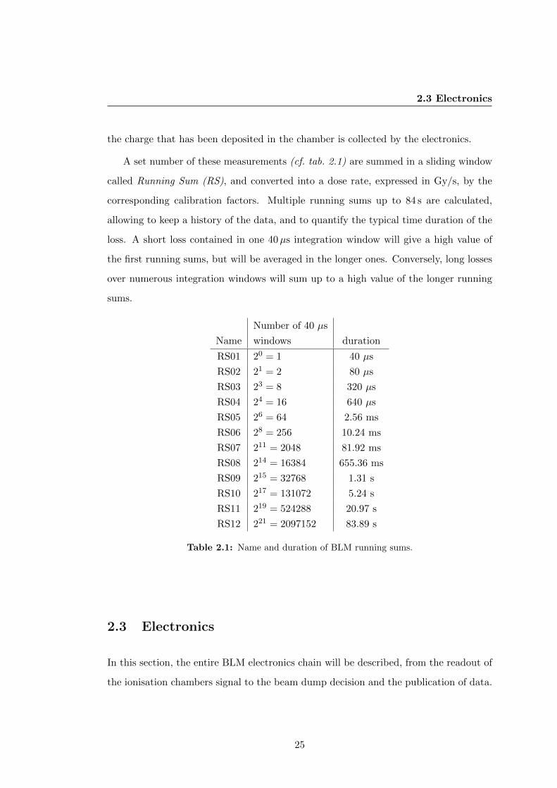
2.3 Electronics
the charge that has been deposited in the chamber is collected by the electronics.
A set number of these measurements (cf. tab. 2.1) are summed in a sliding window
called Running Sum (RS), and converted into a dose rate, expressed in Gy/s, by the
corresponding calibration factors. Multiple running sums up to 84 s are calculated,
allowing to keep a history of the data, and to quantify the typical time duration of the
loss. A short loss contained in one 40µs integration window will give a high value of
the first running sums, but will be averaged in the longer ones. Conversely, long losses
over numerous integration windows will sum up to a high value of the longer running
sums.
Name
Number of 40 µs
windows duration
RS01 20 = 1 40 µs
RS02 21 = 2 80 µs
RS03 23 = 8 320 µs
RS04 24 = 16 640 µs
RS05 26 = 64 2.56 ms
RS06 28 = 256 10.24 ms
RS07 211 = 2048 81.92 ms
RS08 214 = 16384 655.36 ms
RS09 215 = 32768 1.31 s
RS10 217 = 131072 5.24 s
RS11 219 = 524288 20.97 s
RS12 221 = 2097152 83.89 s
Table 2.1: Name and duration of BLM running sums.
2.3 Electronics
In this section, the entire BLM electronics chain will be described, from the readout of
the ionisation chambers signal to the beam dump decision and the publication of data.
25

2. THE BLM SYSTEM
2.3.1 In the tunnel
The output of the ionisation chamber is connected to the front-end electronics, typically
via coaxial cables (cf. fig. 2.5). In places where the front end has to be far away from the
monitors (up to 800 m on the right side of the point 3 of the LHC), a twisted multi-wire
cable is used. The chamber behaves like a capacitor discharging in an analog circuit
called Current to Frequency Converter (CFC) (cf. fig. 2.4).
Figure 2.4: Left: schematics of the Current to Frequency Converter (CFC). The input current
iin(t) corresponds to the charge coming out of the ionisation chamber; the output is the frequency
fout. Right: output of the threshold comparator. The period T changes with time: fout(t) ≡ 1T (t)
.
The first part of the CFC is an integrator in which the charge is integrated into
a current coded by a voltage. While the current is integrated, the voltage builds up,
until it reaches the threshold. At this point, the integrator is quickly (with respect to
the integration time) reset by sending in a reference current Iref (the time needed to
reach the original value is ∆T ). This corresponds to one CFC count. The more charge
comes out of the chamber, the more often the threshold is reached, and the higher the
frequency of counts will be.
This circuit allows continuous operation by not having any dead time. Even if
there is an input current during the reset of the integrator, it is measured: it decreases
the reference current, meaning that the thresholds will be reached faster at the next
“period”, which will consequently be shorter (higher frequency).
26

2.3 Electronics
During one period (cf. fig. 2.4), the reference current Iref can be seen as the slope
of the voltage function during reset: after ∆T , the voltage has increased by ∆Va:
∆Va = Iref ·∆T
If there is an input current during the reset, the reference current is decreased, and the
equation becomes:
∆Va = (Iref − iin) ·∆T (2.1)
The same can be considered during the integration of the signal, which lasts T−∆T .
The input current is the slope of the voltage function:
∆Va = iin · (T −∆T )
T =∆Vaiin
+ ∆T
(2.1 ⇒ T =(Iref − iin) ·∆T
iin+ ∆T
T =Iref ·∆T
iin(2.2)
The output frequency is calculated from there:
fout =1
T=
iinIref ·∆T
(2.3)
This circuit can’t measure negative currents: this would lead to an increase of
voltage in the comparator up to the saturation of the amplifier (cf. fig. 2.4). In order
to avoid this situation, the CFC is equipped with current source of 10 pA, injected
constantly at the input. This value corresponds to the measured average noise value.
This has to be taken into account when considering low losses: no current smaller
than 10 pA can be measured, and subsequently no loss corresponding to a current
lower than 10 pA can be measured. In addition, if the amplifier stays in saturation
mode for more than ∼ 2 min, the CFC has a negative current compensation procedure
(not represented), which increases the offset (up to 255 pA) until the measured current
reaches 10 pA.
The output frequency is acquired and digitized by a Field Programmable Gate
Array (FPGA), which controls an Gigabit Optical link Hybrid (GOH), sending the
data back to the surface via optical fibres. In order to avoid any information loss, these
optical links are redundant: two independent optical links send the same information.
27

2. THE BLM SYSTEM
Figure 2.5: Schematics of the entire electronics chain of the BLM system. The locations and
distances are indicated on the figure.
28

2.4 Thresholds
2.3.2 On the surface
The data processing and evaluation of the measured signal takes place in the Threshold
Comparator cards, on the surface (cf. fig. 2.5). The optical receivers are installed on a
physically separated “mezzanine” card, which is directly plugged on the surface card.
This allows easy replacement and checks.
The values are converted into dose rate (Gy/s) with the corresponding calibration
factors and combined into running sums (cf. tab. 2.1). All values are compared with
the corresponding thresholds, which are different for every running sum and for every
one of the 32 beam energy level, to follow the evolution of the beam in energy in the
machine during the ramp. If any threshold is exceeded, a beam request is sent to the
Beam Interlock System (BIS), and the content of the buffers is saved as post-mortem
data.
Some of these measured running sums are saved in the LHC databases: one value
per running sum is recorded every second. For all running sums shorter than one second
(up to RS08), only one value is logged: the highest loss of all integration windows during
the last second. For the longer running sums, the last in date at the time of logging is
saved (10), even if the value is refreshed more than once per second.
2.4 Thresholds
In the threshold comparator cards, the different running sums are continuously com-
pared with a set of predefined thresholds. If any of the thresholds is exceeded, a beam
extraction is requested via the Beam Interlock System (BIS). The abort thresholds can
be set separately for each BLM, and there are 12 running sums × 32 energy levels.
The threshold for a specific BLM depends on different factors, such as its position
with respect to the beam line and the element it protects, and this element itself. The
setting of the thresholds depends largely on empirical measures, and cannot be fully
verified by automatic test procedures (11). The BLM master thresholds represents the
best knowledge of quench or damage levels. It can be written as:
Th(Eb,∆t) = QBLM (Eb)×Np(Eb,∆t) (2.4)
29

2. THE BLM SYSTEM
where Eb is the energy of the beam, ∆t is the loss duration, QBLM is the signal observed
in a BLM due to a single lost proton, and Np is the maximum number of protons that
can be lost in the protected element.
The time dependence comes from the considerations on loss durations: e.g., some
energy deposited over a long time in one point of a superconducting magnet will have
time to dissipate by conduction, and will be removed by the helium cooling; the same
energy, lost over a very short period, could damage the magnet before the cooling has
any effect. Many other considerations are taken into account, depending on the time
scale of the loss at the considered element. From shorter to longer, the considered
effects are: the heat reserve of the cable, the heat flow between the cable and the
Helium, the Helium heat reserve and the Helium heat flow.
The energy dependence comes from the development of the hadronic shower, which
depends on the energy of the protons. In addition, the superconductivity of a magnet
depends on a set of three interdependent parameters: temperature, current and mag-
netic field. For increasing beam energies, the magnetic field and the current need to
increase as well, leading to tighter limits on the temperature value.
Both QBLM and Np rely strongly on Monte Carlo simulations and therefore include
theoretical uncertainties. Security margins are set to account for these uncertainties,
and they are corrected by analyzing data from the standard operation of LHC and by
performing measurement with specific beam, for instance during machine development
periods.
The values set in the electronics are called applied thresholds, and are always lower
than or equal to the master thresholds:
th(Eb,∆t) = MF × Th(Eb,∆t) (2.5)
where the Monitor Factor MF is chosen lower than one (typically 0.1). It can be chosen
independently for each monitor.
30

2.5 Justification of the doctoral work
2.5 Justification of the doctoral work
As described in § 2.1.2, the installation locations of the BLMs were carefully selected.
Each one of them is associated with a specific element and an expected loss location
within an element. There are many BLMs around the LHC ring, nearly 4000 in total,
including 3600 ionisation chambers.
Nevertheless, each BLM gives just one “local” value: the loss that occurred at the
location where the BLM is installed. In order to gain knowledge about the origin of
a loss, one must consider the element protected by the BLM. For instance, losses at
collimators are to be expected, as it is the role of collimators to create a safe location
for losses.
The collimator characteristics would then help describing the specifics of the loss:
from which plane it originated, if the particles are primary or secondary, and other sim-
ilar information. As another example, a signal in the BLM associated to a quadrupole
would point towards the likely loss location associated to this BLM. The local devel-
opment of a loss, up to the scale of a quadrupole, is fairly well studied.
However, the BLM signals had never been considered on a global scale: that is,
how would a loss develop over dozens of BLM and hundreds of meters. Considering
many BLMs at the same time, and the respective signals in these BLMs, supplementary
information about the origin of the loss can be extracted.
The point of this doctoral work is to try to define what information can be gained
from a more global approach to the losses, and to evaluate the possibilities and the
qualities of these various extractions. Different patterns were used in this work, as well
as different techniques to extract these patterns from the loss profiles. The patterns
included the time evolution of the losses, as well as the spatial distribution – always
considering several monitors at a time.
The feasibility of such a global scale study of the LHC beam losses was evaluated,
and the different techniques fulfilling the goal were developed and tested on real data.
The theory, the implementation and the conclusions on the results will be presented in
the next chapters.
31

2. THE BLM SYSTEM
32
Chapter 3
Principle of Vector
Decomposition
In this chapter, we will explain the need for vector decomposition, and present the
different techniques used in this work.
3.1 Principle
3.1.1 Motivation
The goal of this PhD is to understand the cause of beam losses in the LHC by studying
the loss patterns. One way to achieve this is by reverse engineering: to try to recog-
nize some well-known loss scenarios in a measured loss profile, and to decompose the
measured loss profile as a linear combination of known scenarios. The quality of the
recomposition must be evaluated.
3.1.2 Vector space
Let’s consider an ensemble of m monitors, and a vector space of dimension m. Each
monitor is associated with one dimension (one coordinate) of the vector space. The
ensemble of monitors corresponds to the canonical basis of the space. Any loss profile
can then be expressed as a vector on this space: each of the m coordinates of this
vector is the value of the loss recorded by the corresponding monitor. The losses are
only positive: “negative” losses are not physical. The vector will thus have only positive
coordinates.
33

3. PRINCIPLE OF VECTOR DECOMPOSITION
Let’s consider a group of n known loss scenarios, and the corresponding n vectors
(~vi) expressed on the m-dimensional vector space. In this work, there are only a few
loss scenarios for many monitors: n < m. If the situation was inverted, and there
were more vectors than monitors (n ≥ m), the vectors could be combined to create
a square matrix, that could then be analytically inverted rather simply. It is not the
case here: the vectors only span a subspace of the original m-vector space. They form
a spanning set of the subspace. They are a basis of the n-vector space: typically, they
are independent (this is checked by calculating the determinant) but not orthogonal.
Let’s also consider a measured loss profile, and the corresponding measured vec-
tor ~X.
In order to compare the different vectors, and to make all linear algebra operations
easier, the choice was made to normalize the vectors so that they all have an euclidean
norm equal to 1 in the m-vector space. A vector ~v of the vectors (~vi), is simply divided
by the value ‖~v‖ of its euclidean norm, calculated as:
‖~v‖ =
√√√√ m∑j=0
v2j (3.1)
where the scalars (vj) are the coordinates of the vector ~v.
3.1.3 Vector decomposition
The idea here is to find a linear combination of the vectors (~vi) that will recompose the
vector ~X :n∑i=0
fi · ~vi ≈ ~X (3.2)
where the factors (fi) are the scalars of the linear combination. They form a vector of
dimension n, noted ~F . Note that the recomposition is not exact, because the reference
vectors ~vi are not a basis of the m-vector space. The idea is to find some “typical loss
scenarios” that would compose the considered loss. “Subtracting” a typical loss scenario
from the overall loss is not physical, so the factors have to be positive: ∀i, fi ≥ 0.
The series of operations needed to find a set of factors recomposing the vector ~X
is called vector decomposition. It can be achieved through projections, or matrix in-
version, or some dedicated algorithm. Projections and matrix inversion will be quickly
introduced; then, the corresponding technique used here will be described into greater
details.
34

3.1 Principle
3.1.4 Projections
One way to achieve the vector decomposition (to find the factors of the linear com-
bination) would be to project the measured vector ~X on the vectors (~vi). However,
the vectors (~vi) are not in sufficient number (n < m): they don’t form a basis of the
m-vector space. They form a basis of the n-vector space, and the orthogonal projection
of ~x on this space can be calculated. This is the vector part of the n-vector space which
is the closer to ~X.
One of the simplest processes that can create an orthogonal basis from a non-
orthogonal set of vectors is called the Gram-Schmidt process (cf. § 3.3). It uses no
matrix inversion, no transformation, only simple operations (projection and subtrac-
tion) on the vectors. It can be seen as a geometrical process.
3.1.5 Matrix inversion
Another way to achieve the vector decomposition (to find the factors of the linear
combination) would be to express the equation 3.2 as a matrix equation:
Mm×n · ~Fn ' ~Xm (3.3)
where Mm×n is the matrix of size m×n formed by the n known vectors (~vi), and where
we want to find ~Fn, the n factors of the decomposition. The matrix M needs to be
inverted such that:
~Fn 'M−1n×m · ~Xm (3.4)
Note that the M−1 notation is abusive: it is not exactly an inverse matrix, since it is
not square. The matrix M−1 is the “left inverse” of M : it satisfies M−1 ·M = In but
can not satisfy M ·M−1 = Im (where In is the unitary matrix of size n×n). Note that
the inversion is exact; only the recomposition is not: ~X has no reason to belong to the
subspace generated by the vectors of M .
Once M is inverted and ~F is calculated, the recomposition can be estimated. The
inversion was exact, but the recomposition is not exactly ~X: it is noted ~X ′ and belongs
to the subspace, whereas ~X doesn’t. It is calculated by:
~X ′ = M · ~F (3.5)
35

3. PRINCIPLE OF VECTOR DECOMPOSITION
The error on the vector decomposition can be estimated by calculating the norm of
the difference between the original vector ~X and its recomposition ~X ′:
e ≡ || ~X − ~X ′|| (3.6)
3.2 Singular Value Decomposition (SVD)
The Singular Value Decomposition (SVD) is the generalisation of the diagonalization
of a square matrix, for a non-square matrix. It is a matrix decomposition technique
(into singular values) that allows a simpler inversion of the matrix M than calculating
M−1 directly. The goal is to do a vector decomposition of the vector ~X (finding the
factors).
3.2.1 Principle
The diagonalization of a square matrix is the idea that a diagonalizable square matrix
M can be expressed as the product of three matrices:
M = U · S · U−1
where U is the matrix of eigenvectors; and S is a diagonal matrix where the values
are the eigenvalues associated to the eigenvectors in U , in the same order.
A non-square matrix can be decomposed into singular values. It is called Singular
Value Decomposition (SVD), and is calculated by a computational technique (algo-
rithm) of high precision (cf. § 4.6). The decomposition is exact only to the precision
of the algorithm, but we will assume here that it is exact.
Mm×n ≡ Um×m · Σm×n ·W Tn×n (3.7)
where:
� M is the original matrix, of size m× n;
� U is an orthogonal unitary matrix, of size m×m;
� W is an orthogonal unitary matrix, of size n× n;
� Σ is a non-square diagonal matrix, of size m× n.
36

3.2 Singular Value Decomposition (SVD)
∣∣∣∣∣∣∣∣∣∣
(~v1) · · · (~vn)∣∣∣∣∣∣∣∣∣∣
︸ ︷︷ ︸
Mm×n
=
∣∣∣∣∣∣∣∣∣∣
(~u1) · · · · · · (~um)∣∣∣∣∣∣∣∣∣∣
︸ ︷︷ ︸
Um×m
·
λ1 0 · · · 0
0 λ2 · · · 0...
.... . .
...
0 0 · · · λn
0 0 · · · 0...
......
0 0 · · · 0
︸ ︷︷ ︸
Σm×n
·
—(~w1)—
...
—(~wn)—
︸ ︷︷ ︸
WTn×n
Figure 3.1: Structure of the matrices in the decomposition. M is the original matrix,
made of the vectors (~vi); U and W are the matrices of the left and right singular vectors
respectively. Σ is a diagonal matrix (with n < m) holding the Singular Values: all values
are null, apart from the diagonal λi = (Σ)i,i.
Σ is such that only the diagonal elements are non-null, and there are n in total. These
values (λi) are unique and are called singular values.
U and W are orthogonal matrices: they generate an orthogonal basis of the cor-
responding N -vector space (N = n or m). They satisfy U · UT = IN . The vectors of
U are called left singular vectors, and the ones of W are right singular vectors. These
vectors are not unique for the SVD of one matrix M .
The transformation associated to the matrix M is decomposed by the SVD into
three steps: a rotation (matrix W ), a stretching (matrix Σ) and another rotation
(matrix U) (12).
3.2.2 Advantages
The Singular Value Decomposition calculates the singular vectors U and W as well as
the values λi of Σ. The vectors of U , of dimension m, are orthonormal and form a
basis of the m-vector space, in which the losses are decomposed. Moreover, only the n
first vectors at most are used: there are only n values λi. All vectors (~uj) for j > n are
associated with a zero in Σ during the matrix multiplication.
The singular values in Σ are sorted in decreasing order. The lower λi, at higher
i, can be ignored for faster recomposition at the price of a small error. In this work
n � m, so no λi are omitted. The first vectors (ui) of U , associated to the λi of
37

3. PRINCIPLE OF VECTOR DECOMPOSITION
higher value, will have a strong contribution in the recomposition; the ones with higher
i (i < n) will have a small contribution (λi of smaller value); the ones with i > n will
have no contribution.
3.2.3 Important observations
In this section, we will give the exact expression of the coefficients of M as calculated
by the SVD. The coefficients of the matrices are written in their standard form: (wij)
for the matrix W , where i is the line number and j the column number, both varying
between 0 and n. Note that the vector (~w1) will then have the coefficients (w1j).
The product between the matrices Cm×n and Dn×p, the result is a matrix of coef-
ficients (eij) expressed as:
∀i, j : eij ≡n∑k=1
cik dkj (3.8)
Let’s start by the multiplication Um×m · Σm×n. The elements will be called (sij)
and are:
sij =
m∑k=1
uik λkj
The elements λkj are null for all k > n and all j 6= k, so the intermediate result is:
sij =n∑k=1
uik λkj = uij λj
Now, let’s consider the multiplication of (UΣ)m×n by Wn×n. Eq. 3.8 gives:
mij =n∑k=1
sik wkj =n∑k=1
uik λk wkj
mij =
n∑k=1
λk uik wkj (3.9)
The most important point here is that only the first n vectors (~uk) are used. The
coefficients of M are decomposed into the equivalent of a matrix product of the first n
vectors of U and the vectors of W , but each term of the sum is weighted by a factor λk.
As a consequence, the vectors (uk) for k > n do not take part of the decomposition;
so they are left by the algorithm as canonical vectors: the kth coordinate is 1 and all
the others are zero.
38

3.2 Singular Value Decomposition (SVD)
3.2.4 Pseudoinverse
Once the matrix Σm×n has been created, the pseudoinverse can be created. It is noted
Σ+ and has a size of n × m. All values are null, apart from the diagonal ones which
are (Σ)i,i = 1λi
for λi 6= 0. This matrix is called pseudoinverse because it only satisfies
Σ+ ·Σ = In; the product Σ ·Σ+ is a matrix of size m×m, with only the n first diagonal
elements are 1; all the others are zero.
The pseudoinverse of M is then:
M+ ≡W · Σ+ · UT (3.10)
and satisfies:
M+ ·M = (W · Σ+ · UT ) · (U︸ ︷︷ ︸Im
·Σ ·W T )
= W · Σ+ · Σ ·W T
= W ·W T
M+ ·M = In
Note that it is different for M ·M+: for the same reason as Σ · Σ+, it is a matrix
of size m×m, with only the n first diagonal elements are 1; all the others are zero.
3.2.5 Recomposition
Once the pseudoinverse has been calculated, the factors can be calculated (vector de-
composition). The result is not exact, because the vector ~X is generally not part of the
subspace generated by the vectors of M .
M · ~F ' ~X
M+ ·M · ~F 'M+ · ~X
~F 'W · Σ+ · UT︸ ︷︷ ︸M+
· ~X
~F 'M+ · ~X
The recomposition ~X ′ is then calculated by:
~X ′ = M · ~F
~X ′ = M ·W · Σ+ · UT︸ ︷︷ ︸M+
· ~X
39

3. PRINCIPLE OF VECTOR DECOMPOSITION
3.2.6 Limitations
Accuracy of the recomposition
Given the matrix M , the SVD algorithm will always calculate a matrix decomposition
M = U ·Σ ·W T . Once the pseudoinverse M+ calculated, the set of factors ~F can always
be calculated, as well as the recomposition ~X ′. This recomposition is the combination
of the vectors (~vi) which is the closest to ~X, and belongs to the subspace generated by
the vectors of the loss scenarios. However, it doesn’t mean that the recomposition ~X ′
will actually be close to ~X; it can even be null. An example of such a situation is:
M =
1 10 10 0
~X =
001
No set of factors can recompose ~X: the projection of ~X on the subspace generated by
the vectors of M is the point of coordinates (0, 0, 0).
Without a proper evaluation of the accuracy of the vector decomposition, the factors
are meaningless.
Negative factors
In the standard Rm vector space, each factor fi can take any value in R. However, there
are physical limitations. The factors (fi) represent the contribution of the different
“standard” loss profiles (vectors (~vi)): negative values are not physical, nothing would
“remove” a loss profile. Moreover, the losses are only positive: again, negative losses
make no sense. The vectors (~vi) are in (R+)m: the space generated by the positive half
of the field of real numbers (noted R+) considered m times.
A negative factor in the vector decomposition indicates that the corresponding
vector can not contribute to the reconstruction of the vector ~X. This means that
the corresponding vector can not take part of the decomposition. It often points to
a problem in the decomposition, for example that the chosen loss scenarios are not
exactly adapted to the problem, and that the measured vector has other components
than the selected vectors (~vi).
One way to deal with this effect would be to remove this vector from the matrix
M : the matrix would then have a size m− 1. The SVD could be calculated again; the
40
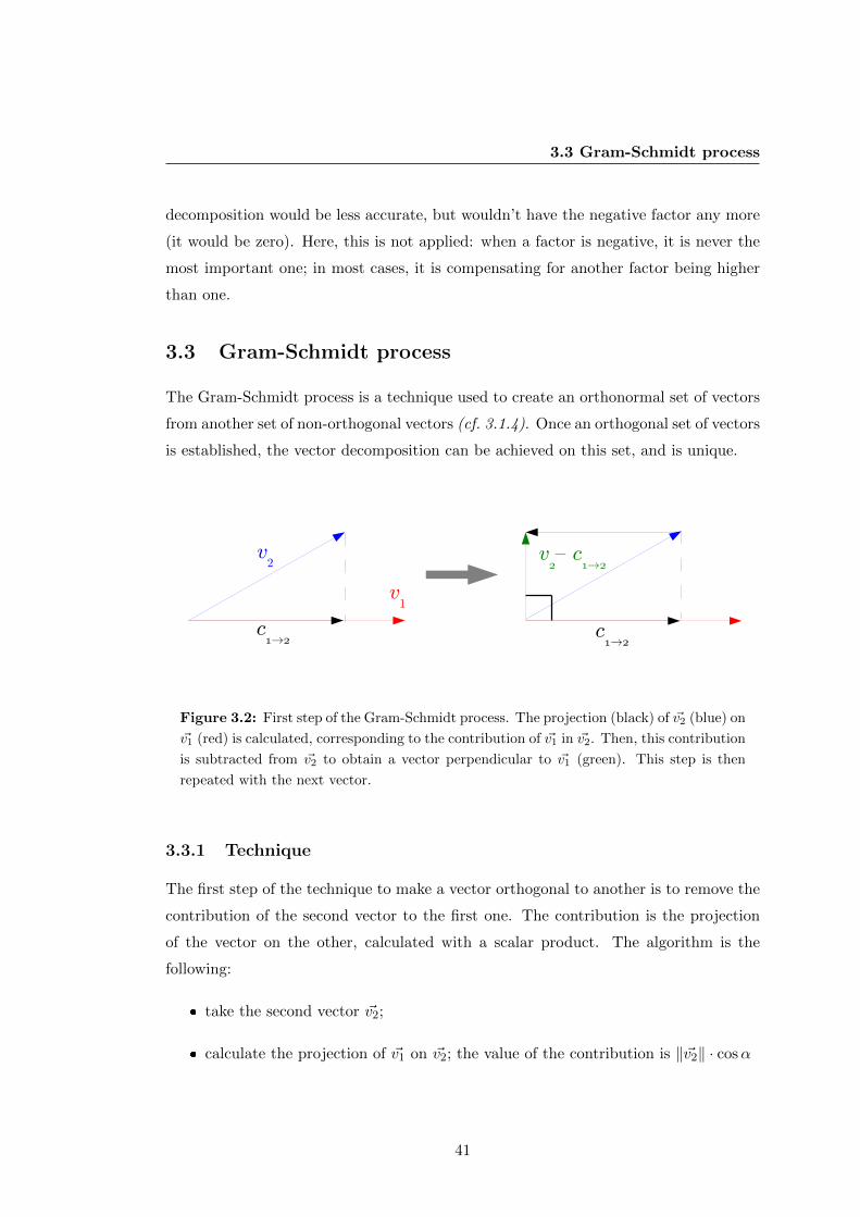
3.3 Gram-Schmidt process
decomposition would be less accurate, but wouldn’t have the negative factor any more
(it would be zero). Here, this is not applied: when a factor is negative, it is never the
most important one; in most cases, it is compensating for another factor being higher
than one.
3.3 Gram-Schmidt process
The Gram-Schmidt process is a technique used to create an orthonormal set of vectors
from another set of non-orthogonal vectors (cf. 3.1.4). Once an orthogonal set of vectors
is established, the vector decomposition can be achieved on this set, and is unique.
v1
v2 { c
1!2
c1!2
v2
c1!2
Figure 3.2: First step of the Gram-Schmidt process. The projection (black) of ~v2 (blue) on
~v1 (red) is calculated, corresponding to the contribution of ~v1 in ~v2. Then, this contribution
is subtracted from ~v2 to obtain a vector perpendicular to ~v1 (green). This step is then
repeated with the next vector.
3.3.1 Technique
The first step of the technique to make a vector orthogonal to another is to remove the
contribution of the second vector to the first one. The contribution is the projection
of the vector on the other, calculated with a scalar product. The algorithm is the
following:
� take the second vector ~v2;
� calculate the projection of ~v1 on ~v2; the value of the contribution is ‖~v2‖ · cosα
41

3. PRINCIPLE OF VECTOR DECOMPOSITION
where ~v1 · ~v2 = ‖~v1‖ · ‖~v2‖ · cosα and cosα =(~v1 · ~v2)
‖~v1‖ · ‖~v2‖so the contribution
of ~v1 in ~v2 is:(~v1 · ~v2)
‖~v1‖· ~v1
‖~v1‖(cf. fig. 3.2)
� subtract the contribution of ~v1 from ~v2: ~v2′ = ~v2 − (~v1 · ~v2) · ~v1
‖~v1‖2
The result is a vector having no contribution on ~v1, i.e. orthogonal to ~v1:
~v1 · ~v2′ = ~v1 ·
[~v2 − (~v1 · ~v2) · ~v1
‖~v1‖2
]= ~v1 · ~v2 − (~v1 · ~v2) · ~v1 · ~v1
‖~v1‖2
= ~v1 · ~v2 − (~v1 · ~v2) · ‖~v1‖2
‖~v1‖2︸ ︷︷ ︸=1
= ~v1 · ~v2 − ~v1 · ~v2
~v1 · ~v2′ = 0
This must be repeated for each vector. Every time, the contribution from all precedent
vectors must be subtracted:
~vi′ = ~vi −
i−1∑j=1
(~vj · ~vi) ·~vj‖~vj‖2
(3.11)
Only the first vector is left unchanged.
The result is a set of vectors (~v′i) where all vectors are orthogonal to the others.
Once this set is created, the measured vector ~X can be decomposed.
3.3.2 Importance of the order of the vectors
During the Gram-Schmidt process, only the first vector is left unchanged. If all vectors
are “close” to each other, as in our case (in the same 12m subdivision of Rm, that is
(R+)m), then the main factor fi in the vector decomposition will be the first one:
~X ' ~v1 ⇒ ~X · ~v1 ' 1
All other vectors of the orthogonal set have to have some negative coordinates in order
to be orthogonal to the first vector (which has only positive coordinates). If the second
42

3.4 MICADO
vector ~v2 only had positive coordinates, it would give a strictly positive scalar product:
∀i, v1i > 0, v2i > 0 ⇒m∑i=0
v1i · v2i > 0
proving that some negative elements in ~v2 are needed to compensate for all strictly
positive elements of ~v1. In short, if all coordinates of ~v1 and ~v2 are strictly positive,
the two vectors can’t be strictly orthogonal. (In this study, this is particularly true for
vectors corresponding to the same beam and transversal planes, e.g. B1H and B1V;
less so for vectors of different beams).
The contribution of the other vectors in the recomposition will then be small. This
can be expressed as:
~v2′ ⊥ ~v1 and ~v1 ' ~X ⇒ ~v2
′ · ~X ' 0
This is a broad simplification, and the results showed that the factors can have
other values than 1 or 0. But the conclusion is that the order in which the vectors
(~vi) are considered when creating the orthogonal set (~v′i) influences the result of the
decomposition.
Since the order of the vectors is chosen, the choice was made to order the vectors
(~vi) by “closeness to ~X” (in the sense of the scalar product) before the Gram-Schmidt
process. The vector ~vi which is the “closest” to ~X (i.e. the one that maximizes ~X · ~vifor all i) will give the highest factor of all (fi): it will also be the highest contribution
in the recomposition ~X ′.
3.4 MICADO
MICADO (standing for “MInimisation des CArres d’Orbite”) is an iterative algorithm
that doesn’t involve any projection or matrix inversion: it calculates the factors (fi)
(vector ~F ) directly (13).
The algorithm starts with an arbitrary set of factors (fi) (vector ~F ); calculates
the recomposition ~X ′ = M · ~F ; and evaluates the quality of the recomposition ‖ ~X ′ −~X‖. Then, it varies the factors, and checks that the new recomposition is closer to
the original vector than the first recomposition. These iterations carry on until the
algorithm converges.
43
3. PRINCIPLE OF VECTOR DECOMPOSITION
3.5 Recomposition and error
3.5.1 Motivation
All the algorithms presented here, when given a set of vectors and a measured vector,
will always return a decomposition of the measured vector on the vector set (cf. § 3.2.6).
A recomposition of the original vector as a linear combination of the basis vectors can
always be calculated (cf. eq. 3.5). This recomposition is the projection of the original
vector on the subspace generated by the reference vectors, and is the “closest” possible
to the original vector.
However, the recomposition has no reason to be actually close to the original vec-
tor: it depends only on the vector set. In some cases, the recomposition can be null
(cf. § 3.2.6).
A way to evaluate the error on the recomposition is needed, in order to know how
accurate the decomposition was.
3.5.2 Evaluation of the error
As seen before (cf. § 3.1.2), all vectors are in (R+)m (the space generated by the positive
half of the field of real numbers (R+) considered m times) which means that they are
“close” to each other in the sense of the scalar product: ∀ ~va, ~vb ∈ (~vi), 0 < ~va · ~vb ≤ 1.
In order to evaluate how close two vectors are in the m-vector space, the choice was
made to consider the norm of the difference (subtraction) between the two vectors
(cf. fig. 3.3):
(eq. 3.6) e = ‖~va − ~vb‖
Note that no claim is made here that this choice is the best; some other ways to
evaluate this difference can be considered, such as normalizing to the highest monitor
instead of normalizing to the vector length; or using different norms than the euclidean
norm (‖x‖2 =√∑
x2j ), for instance: ‖x‖1 =
∑|xj | or ‖x‖∞ = max(xj).
The error on the recomposition is evaluated by calculating the norm of the difference
between the original vector and its recomposition. Since the two vectors are in (R+)m,
the recomposition error has to be between 0 (when the two vectors are equal) and√
2
(when the two vectors are orthogonal).
For SVD, the recomposition is straightforward (cf. § 3.2.5), and has a physical
meaning. The reference vectors are actual loss profiles, and the understanding of the
44

3.5 Recomposition and error
Figure 3.3: Example of the calculation of the error on the recomposition between two vectors
~v1, ~v2, in a space where m = 2. Note that this is always valid, because two vectors always generate
a plane in a m dimensions vector space. The purple dash represent the scalar product ~v1 · ~v2. The
error on the recomposition is the length of the vector ~e.
factors is mathematically exact: they are the coefficients of the linear combination of
loss profiles.
For the Gram-Schmidt process, the recomposition is not as straightforward. The
returned factors are associated to the orthogonalised vectors (after the process) and
not to the reference vectors. The orthogonalised vectors don’t have a direct physical
meaning: they are a reference vectors minus their projections on other reference vectors
(cf. § 3.3). Moreover, the recomposition calculated with the orthogonalised vectors is
exactly the same vector as the recomposition from SVD: it is the projection of the
original vector on the subspace. The error on the recomposition would be exactly the
one calculated for the SVD.
Instead, the choice was made to calculate the error on the recomposition with the
original reference vectors (before orthogonalisation) instead of the orthogonalised vector
used to calculate the decomposition. This choice was motivated by the values of these
errors, which only differ by around 1%. An example of distributions of the errors on
recomposition will be presented in fig. 4.20.
The error on the recomposition for Gram-Schmidt (G-S) is not mathematically
exact – the exact value is given by the one for SVD – but carries a physical meaning
(linear combination of the reference vectors), at the cost of a small error.
45

3. PRINCIPLE OF VECTOR DECOMPOSITION
3.6 Conclusion
The theories of the different techniques of vector decomposition and a way to evaluate
the difference between the original vector and the recomposed vector were presented.
The next chapter will explain the practical details of the implementation of these de-
compositions: which monitors and which vectors were chosen.
46
Chapter 4
Implementation of Vector
Decomposition
This chapter will present the implementation of vector decomposition: the choice of
the known loss scenarios, and the selection of the BLMs that generate the vectors.
4.1 Creation of the default vectors
In this section, the creation of the reference vector set will be presented: which loss
scenarios are used, and how they were gathered.
4.1.1 Choice of beam loss scenarios
The goal of this work is to try to recognize patterns in the LHC beam losses; to adapt
and implement algorithms achieving a decomposition of measured loss profiles into a
sum of known loss scenarios (used as patterns); and to evaluate the quality of these
different decompositions.
The choice was made to start with the typical loss scenarios in the point 7 of
the LHC. It is the place where the primary and secondary collimators for transversal
(horizontal and vertical) cleaning are installed, creating the highest losses in nominal
running conditions (this will be described in the next chapter, fig. 5.1, the default loss
profile in the LHC during nominal operation).
The chosen loss scenarios are the resonance crossings for both planes and both
beams (cf. fig. 4.1). They are the verification measurements of collimation cleaning.
47

4. IMPLEMENTATION OF VECTOR DECOMPOSITION
4 T
CP
s
3 TC
Hs
TC
SG
TC
LA
s
Sig
na
ls on
ve
rtical T
CP
Losses [Gy/s]
BL
M in
dex [n
o u
nit]
Figure 4.1: Example of one set of the 4 transversal loss scenarios for the 4 resonance crossings
(2 planes and 2 beams) measured in the point 7 of LHC. The horizontal axis gives the index of
the BLM, and the vertical axis gives the measured losses for each profile. This set was measured
the 9th of September 2010 (cf. tab. 4.1) and is not used in the final decomposition. All vectors
are normalised so they have a length 1 in the m-vector space. Only the relative position (order) of
the monitors is respected (same as in the LHC), not their absolute position (DCUM). Note that
only a few BLMs present a different signal between horizontal losses and vertical losses (such as
the BLM associated to the vertical TCPs: #18 and #118).
48

4.1 Creation of the default vectors
Each of these verifications is called a loss map. The operator changes the tune Q of
one plane such that it crosses the resonance Q = 13 : the beam size in the corresponding
plane suddenly increases up to the point of touching the primary collimators jaws. The
collimators being in their nominal position, the measured loss map is nominal.
Later, more reference vectors were added. In order to have a more complete under-
standing of the collimation cleaning in the LHC, two transversal loss scenarios were
added, corresponding to the momentum cleaning. This way, the complete set of pri-
mary collimators in the LHC are taken into account. However, the momentum cleaning
is achieved in the point 3 of the LHC, meaning that extra monitors will be added later.
It was also decided to add the BLMs associated to all the tertiary collimators out
of interest. All these monitors were added at the same time, when recalculating the
“longer” vectors (with more coordinates). The choice of monitors and loss maps for
IR3 will be presented separately.
The transversal (horizontal & vertical) loss scenarios have the advantage of present-
ing very different cases. The difference between both beams is very obvious (purple
and blue profiles for Beam 1, black and green profiles for Beam 2 on fig. 4.1), because
the corresponding primary collimators are far away from each other. On the other
hand, the horizontal and vertical scenarios are very entangled. The difference is visible
on the two first primary collimators (cf. fig. 4.1, #18 and #118); the signals down-
stream correspond mainly to disturbed particles and/or secondary showers, which are
very complex. These secondary showers don’t follow the optics of the LHC, and their
propagation on the downstream monitors is similar for both beams.
4.1.2 Dates of measurement
The first transversal loss maps used were all measured in 2010 (cf. tab. 4.1). The dates
of these loss maps were found first by being in the CERN Control Center when they
were measured, and by searching the LHC logbook (14). These dates were cross-checked
in collaboration with members of the Collimation Working Group (CWG) (15). One
date had to be removed because of wrong collimator hierarchy, and two other dates
that had been missed were added. Due to the low number of loss maps, they were all
kept and used.
49
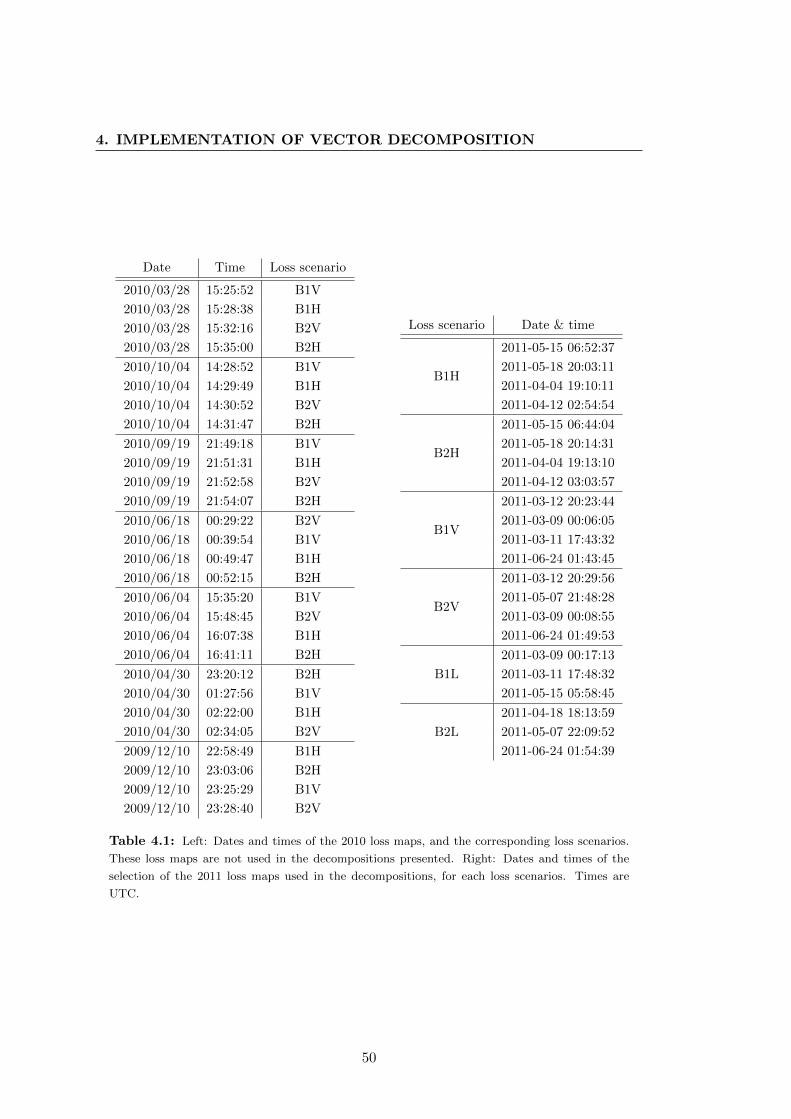
4. IMPLEMENTATION OF VECTOR DECOMPOSITION
Date Time Loss scenario
2010/03/28 15:25:52 B1V
2010/03/28 15:28:38 B1H
2010/03/28 15:32:16 B2V
2010/03/28 15:35:00 B2H
2010/10/04 14:28:52 B1V
2010/10/04 14:29:49 B1H
2010/10/04 14:30:52 B2V
2010/10/04 14:31:47 B2H
2010/09/19 21:49:18 B1V
2010/09/19 21:51:31 B1H
2010/09/19 21:52:58 B2V
2010/09/19 21:54:07 B2H
2010/06/18 00:29:22 B2V
2010/06/18 00:39:54 B1V
2010/06/18 00:49:47 B1H
2010/06/18 00:52:15 B2H
2010/06/04 15:35:20 B1V
2010/06/04 15:48:45 B2V
2010/06/04 16:07:38 B1H
2010/06/04 16:41:11 B2H
2010/04/30 23:20:12 B2H
2010/04/30 01:27:56 B1V
2010/04/30 02:22:00 B1H
2010/04/30 02:34:05 B2V
2009/12/10 22:58:49 B1H
2009/12/10 23:03:06 B2H
2009/12/10 23:25:29 B1V
2009/12/10 23:28:40 B2V
Loss scenario Date & time
B1H
2011-05-15 06:52:37
2011-05-18 20:03:11
2011-04-04 19:10:11
2011-04-12 02:54:54
B2H
2011-05-15 06:44:04
2011-05-18 20:14:31
2011-04-04 19:13:10
2011-04-12 03:03:57
B1V
2011-03-12 20:23:44
2011-03-09 00:06:05
2011-03-11 17:43:32
2011-06-24 01:43:45
B2V
2011-03-12 20:29:56
2011-05-07 21:48:28
2011-03-09 00:08:55
2011-06-24 01:49:53
B1L
2011-03-09 00:17:13
2011-03-11 17:48:32
2011-05-15 05:58:45
B2L
2011-04-18 18:13:59
2011-05-07 22:09:52
2011-06-24 01:54:39
Table 4.1: Left: Dates and times of the 2010 loss maps, and the corresponding loss scenarios.
These loss maps are not used in the decompositions presented. Right: Dates and times of the
selection of the 2011 loss maps used in the decompositions, for each loss scenarios. Times are
UTC.
50

4.1 Creation of the default vectors
Later, in 2011, more loss maps were measured in different conditions, allowing a
finer selection. The different conditions, their effect on the loss maps and the selections
are discussed in § 4.3. The final selection is presented in tab. 4.1.
4.1.3 Normalisation
The overall loss depends on many factors. The most important of them is the beam
intensity, but the losses also depend on the optics: focusing errors are amplified during
the crossing of the 1/3 resonance, leading to an increase of the transversal beam size.
Particles will then be lost on places where the beam envelop is close to the aperture.
The intensity of the overall loss is different for every vector of every set: the vectors
must be normalized before comparison.
The choice was made to normalize the vectors to an euclidean norm of 1 in the
m-vector space: that is, to divide the vector by its length in the sense of the euclidean
norm (the standard norm in a vector space). This is motivated by the concept of an
orthonormal base of the sub-space: here the vectors are not orthogonal, but still have
a norm equal to 1 (cf. fig. 4.2). In most cases, the norm of the vector is dominated by
one or few coordinates, so this is similar to normalising to the highest signal.
4.1.4 Effect of the BLM offset
Even when no particle is lost from the beam, there is always a minimum signal in the
BLMs. This is part of the design: a 10 pA current is permanently sent in the reading
electronics, avoiding the situation where there is no charge to collect (cf. § 2.3). This
can be seen in fig. 4.2, top: all BLMs above index #125 have the same signal for all
dates, even though the losses had different amplitudes. The explanation is that no loss
was recorded at these position, only the offset current. It corresponds to 1.8 ·10−7 Gy/s
for RS09.
When the vector is normalised, the offset is divided by the value of the euclidean
norm of the corresponding vector. It results in various artificial increases of the offset,
as seen in fig. 4.2 bottom for all BLMs above index #125. This could have an effect on
the decomposition: during a globally low loss, the affected monitors would present a
normalised signal higher than for a globally high loss, even if their signals were originally
equal (and null).
51

4. IMPLEMENTATION OF VECTOR DECOMPOSITION
Figure 4.2: Example of the effect of the normalisation. Both plots show the loss maps (measured
at different dates in 2010) of one loss scenario: the vertical resonance crossing of beam 2. These
specific loss maps are not used in the decomposition. Top: the vectors are not normalized. The
“shapes” (the respective values of the coordinates) are similar, but the euclidean norm is different.
Bottom: all vectors have a euclidean norm equal to one. The “shapes” are similar for all vectors.
The BLMs on the right (above #125) show the effect of normalisation on the offset: they had
the same signal (1.8 · 10−7 Gy/s) for all curves before normalisation (top), but show different
normalised signals (bottom). Therefore, the value of the offset is subtracted from all BLM signals
before normalisation.
52

4.2 Choice of the list of BLMs
In order to avoid this phenomenon, the value of the offset (1.8 · 10−7 Gy/s for
RS09) is systematically removed from all monitors when constructing the vectors, before
normalisation.
4.2 Choice of the list of BLMs
This section will present the selection of the m BLMs from IR7 composing the coordi-
nates of the transversal loss vectors expressed in the m-vector space. The selection of
monitors of IR3 will be presented separately.
4.2.1 Problem
In this work, each coordinate of the loss vectors corresponds to the signal of one BLM.
They must be selected following specific criteria. Beforehand, these criteria themselves
must be established.
The influence of each BLM signal — each vector coordinate — on the whole vector
depends only on the intensity of the loss, and BLMs with high losses will have a higher
weight in the decomposition. In addition, the point of this work is to separate different
loss vectors (loss scenarios). From this point of view, there are three main types of
monitors:
1. BLMs that have a low signal in all loss scenarios;
2. BLMs that have a high signal in all loss scenarios;
3. BLMs that have different signals in different loss scenarios.
It is obvious that the most interesting BLMs, when discriminating between scenar-
ios, will be the BLMs of the third type.
BLMs with low signal in all scenarios
When calculating one of the vector decompositions, the BLMs of the first type have
no influence. They do not carry information on the nature of the loss: if added to the
vectors, they only “dilute” this information. If they are included, the vector will have
a higher dimension for the same information.
53

4. IMPLEMENTATION OF VECTOR DECOMPOSITION
It is better to ignore these BLMs. Tests on simple examples show that they don’t
drastically change the result of a decomposition. Typically, for SVD, one of the left
eigenvectors will have zeros everywhere, and a one at the position of the BLM: it will
be a vector of the canonical basis. The corresponding singular value will be very low, or
there will be no singular value associated to that vector: the index of the vector will be
higher than n. The vector will either be ignored or have only a negligible contribution.
This was checked by running the SVD with all monitors in IR7, then plotting all the
left singular vectors of matrix U (cf. § 3.2).
BLMs with high signal in all scenarios
The case opposite to BLMs of the first type are the BLMs that show, in every case, a
signal higher than most other BLMs of the vectors. This case is more critical because
such BLMs, even if they cannot be used for discriminating between loss scenarios, have
a strong influence on the decomposition: the higher the signal of the BLM relative to
the others, the higher the influence on the decomposition. Only a small variation on
the contribution of such BLMs can be bigger than the signal of some other BLMs, and
lead to a change in the recomposition result.
If possible, such BLMs should be removed from the list, as they do not carry dis-
criminating information: their signal is high in all scenario. They could lead to wrong
decomposition. The concept of the decomposition is to match vectors. Between all
coordinates, the highest ones have the highest influence on the decomposition. Match-
ing such a coordinate (even if it carries no information) to the detriment of a another
smaller coordinate (which could carry information) will lead to a smaller error on the
decomposition for the wrong information. The vector would have been matched to the
“wrong” coordinate.
BLMs that have different signals in different scenarios
This third case is the most relevant one. These BLMs can be used for simple discrimi-
nation “by eye” between scenarios. They are the BLMs carrying the information about
the differences between the loss scenarios.
The selected BLMs were the ones that were at the same time in the list of BLMs
with highest signals, and in the list of BLMs with the highest variations from one loss
54

4.2 Choice of the list of BLMs
scenario to another. The ways to evaluate this variation are presented in the next
section.
4.2.2 Selection technique
The list of chosen BLMs, selected after sorting by different criteria, was produced by
following several steps.
Distributions of the signal of each BLM
For the BLM selection, all loss scenarios were considered together. All the occurrences
(loss maps) of all the loss scenarios were gathered. Each loss map is a verification
measurement of collimation cleaning. These measurements are done on a regular basis
in the LHC, meaning that several are available.
The average signal and the standard deviation of each BLM were calculated consid-
ering all loss maps of all scenarios together, after normalisation. The standard deviation
gives a quantification of the variation of the signal from one loss scenario to another.
Beforehand, the check was made that the signal of one BLM doesn’t change much
between loss maps of the same scenario (cf. § 4.1.1). The standard deviation of the
signal of a BLM within one loss scenario is small: less than 5% of the average signal,
for 2010 and 2011 loss maps. Conversely, the standard deviation between scenarios is
big (cf. fig. 4.3): same order of magnitude as the average; that is, much bigger than
the standard deviation within one scenario.
Variations of BLM signal between scenarios
The first way to evaluate the variation of one BLM signal from one scenario to another
was to calculate the difference between the highest and the lowest signal for all loss
maps. However, this doesn’t take into account all loss maps, only the two loss maps
with highest and lowest signal. The way to consider all loss maps is to use standard
deviation.
However, both the standard deviation and the difference between minimum and
maximum signals are proportional to the mean value of the signal. When ordering
the monitors by decreasing standard deviation, the results are extremely similar as a
simple “ordering by signal” (cf. tab. 5.1). The relevant quantities here are the Relative
55

4. IMPLEMENTATION OF VECTOR DECOMPOSITION
Figure 4.3: Distributions of all BLMs of point 7 when considering all loss scenarios at the
same time, for the loss maps of 2010. Averages and standard deviations are calculated for all 28
measurements (4 scenarios × 7 dates) at the same time. These specific loss maps are not used
in the decomposition, but the selection is the same. BLMs are displayed with the same relative
order as they have in the LHC, but DCUM is not respected. The BLMs showing the bigger error
bars are the most relevant ones.
Standard Deviation (RSD); and the min/max ratio, which corresponds to the “length
of the error bar” in log scale (cf. fig. 4.3).
These two quantities gave very similar results, and the monitors with the highest
values were selected (cf. tab. 4.2).
Symmetry beam 1 / beam 2
The physical implementation of components and instruments in the LHC is nearly
always symmetric for beam 1 and beam 2 around the interaction points. It is the case
for the collimators in point 3 and 7. In order to follow this symmetry, every time a
monitor was selected for one beam, the symmetric monitor was added to the list as
well. This is validated by the fact that in most cases, both monitors were already in
the selection.
The results are presented in tab. 4.2.
56

4.3 Final loss map selection
Index BLM left of IP 7 Symmetric BLM right of IP 7 Index
018 BLMEI.06L7.B1E10_TCP.D6L7.B1 BLMEI.06R7.B2I10_TCP.D6R7.B2 114
019 BLMEI.06L7.B1E10_TCP.C6L7.B1 BLMEI.06R7.B2I10_TCP.C6R7.B2 113
020 BLMEI.06L7.B1E10_TCP.B6L7.B1 BLMEI.06R7.B2I10_TCP.B6R7.B2 112
021 BLMEI.06L7.B1E10_TCP.A6L7.B1 BLMEI.06R7.B2I10_TCP.A6R7.B2 111
022 BLMEI.06L7.B1E10_TCHSV.6L7.B1 BLMEI.06R7.B2I10_TCHSV.6R7.B2 110
023 BLMEI.06L7.B1E10_TCHSH.6L7.B1 BLMEI.06R7.B2I10_TCHSH.6R7.B2 109
024 BLMEI.06L7.B1E10_TCHSS.6L7.B1 BLMEI.06R7.B2I20_TCHSS.6R7.B2 108
026 BLMEI.06L7.B1E10_MBW.B6L7 BLMEI.06R7.B2I10_MBW.B6R7 106
030 BLMEI.06L7.B1E10_TCSM.A6L7.B1 BLMEI.06R7.B2I10_TCSM.A6R7.B2 100
054 BLMEI.04L7.B1E10_TCSG.D4L7.B1 BLMEI.04R7.B2I10_TCSG.D4R7.B2 77
055 BLMEI.04L7.B1E10_TCSM.D4L7.B1 BLMEI.04R7.B2I10_TCSM.D4R7.B2 76
007 BLMEI.07L7.B2I10_TCLA.A7L7.B2 BLMEI.07R7.B1E10_TCLA.A7R7.B1 125
010 BLMQI.06L7.B2I20_MQTL BLMQI.06R7.B1E20_MQTL 122
012 BLMQI.06L7.B2I10_MQTL BLMQI.06R7.B1E10_MQTL 120
013 BLMEI.06L7.B2I10_TCLA.D6L7.B2 BLMEI.06R7.B1E10_TCLA.D6R7.B1 119
014 BLMQI.06L7.B1E30_MQTL BLMQI.06R7.B2I30_MQTL 118
015 BLMEI.06L7.B2I10_TCLA.C6L7.B2 BLMEI.06R7.B1E10_TCLA.C6R7.B1 117
028 BLMEI.06L7.B2I10_TCLA.B6L7.B2 BLMEI.06R7.B1E10_TCLA.B6R7.B1 107
031 BLMEI.06L7.B2I10_TCLA.A6L7.B2 BLMEI.06R7.B1E10_TCLA.A6R7.B1 101
040 BLMEI.05L7.B2I10_TCSM.E5L7.B2 BLMEI.05R7.B1E10_TCSG.E5R7.B1 91
051 BLMEI.05L7.B2I10_TCSM.A5L7.B2 BLMEI.05R7.B1E10_TCSM.A5R7.B1 80
Table 4.2: List of selected BLMs of IR7. The index corresponds to the BLM index in the figures
showing the signal distributions, such as fig. 4.1, fig. 4.2 and fig. 4.3. The monitors were selected
to have the highest relative standard deviation, or to be the symmetric of such a monitor. In the
naming convention, the part after the underscore “ ” is the name of the element associated to the
BLM; the part before describes the BLM and its position.
4.3 Final loss map selection
In 2011, following the experience acquired in 2010, the settings of the collimators were
changed, and in the first months of 2011, many loss maps were measured. The first
observation were that these loss maps were different from the ones measured in 2010.
They also show differences in shape one to another.
4.3.1 Dependency on energy
The settings (opening of the jaws) of the collimators being dependent on the energy, the
loss profiles will be different depending on the energy. Within all loss maps measured
in 2011, two different beam energies were used. The loss maps were sorted according to
57

4. IMPLEMENTATION OF VECTOR DECOMPOSITION
Figure 4.4: All 2011 loss maps (at the time of the study) for Beam 1 horizontal, normalised.
Note that even though the overall shapes are similar, critical monitors such as the ones associated
to primary collimators give “inconsistent” results: the loss at the vertical collimator (#18) in one
loss map can be the same as the value at the horizontal collimator (#19) in another loss map.
whether the loss map was measured at injection energy (450 GeV) or collision energy
(3.5 TeV at the time). One example for the loss scenario B1H is shown in fig. 4.4.
However, even after sorting by energy, the results are still “inconsistent”: even
though the overall shapes are similar, the variations of the loss recorded in one BLM
within one loss scenario are in some cases higher than the signal of the BLM. For
instance, the BLMs at index #18 and #19 can have similar values from one loss map
to another. Sorting by energy is not enough.
The loss maps must be sorted according to another criterion: the order in which
they were measured.
58

4.3 Final loss map selection
Figure 4.5: Top: 2011 loss maps for B1H measured before the loss maps for B1V. Bottom: 2011
loss maps for B1H measured after the loss maps for B1V. Each colour correspond to a different
loss map. Note how the spread is different: the normalised losses for one BLM are very close in
the first case, and further apart in the second. Quantitative values of standard deviation are given
in Fig. 4.6.
59

4. IMPLEMENTATION OF VECTOR DECOMPOSITION
4.3.2 Order of the loss maps
As described in § 4.1.1, the loss maps are measurements of losses during the crossing
of the resonance of the tune for one of the transversal planes. The measurement for the
other plane is done directly afterwards: the beam is not extracted, and no new beam
is injected.
However, the resonance crossing and the cleaning by the collimators perturb the
beam. Even though it is supposed to affect only one plane, both planes see an effect,
even if it is only due to the coupling between them. This means that the loss maps
corresponding to the plane measured first will give very consistent and reproducible
results, whereas the loss map measured secondly will be perturbed.
This effect is shown in fig. 4.5. The loss maps all correspond to the same loss
scenario (beam 1 horizontal), and they are sorted according to the following criterion:
whether the loss maps were measured before or after the other loss scenario for the
same beam (beam 1 vertical). The difference can already be estimated visually: there
is more variation within the values of one monitor when the loss maps were measured
in second position (cf. fig. 4.5 bottom).
4.3.3 Reproducibility for IR7
Quantitative result are given in fig. 4.6. It shows the loss maps for beam 2 horizontal
which were measured before the loss maps for beam 2 vertical. For each of the selected
monitors, the standard deviation was calculated and normalised by the average signal.
The results are shown in blue: most monitors have a standard deviation corresponding
to 1% of the average signal.
These loss maps were measured over the course of three months, showing that during
this period, the standard deviation of the BLM signal (after vector normalisation) is
around 1% of the average signal (cf. fig. 4.6).
4.4 Adding more cases: longitudinal scenarios and TCTs
Once the standard vectors for the insertion region 7 were assumed to be correct, the
decision was made to extend the analysis by adding information about the third beam
plane: the longitudinal cleaning of the beam. The collimators for longitudinal cleaning
are installed in insertion region 3.
60

4.4 Adding more cases: longitudinal scenarios and TCTs
Figure 4.6: Values of signals in all monitors of IP7 for the B2H loss maps of 2011, and values of
the normalised standard deviation of the signal of the selected BLMs (in blue), for all loss maps of
the loss scenario B2H taken before the loss maps for B2V. All scenarios and the final selection of
monitors will be presented in fig. 4.11, fig. 4.12 and fig. 4.13. Most of the standard deviations are
around 1% of the value of the average. The two higher values (#122 and #125) appear because
the average value of the signal for this scenario is small and close to the offset, and the effect of
the noise gives a high standard deviation. These monitors were selected by symmetry and are not
relevant for B1 scenarios; the symmetric monitors, which are used in this scenario, are at index
#7 and #12, and have a normalised standard deviation around 1% as well.
In this section, we will present the different problems which arise when adding the
longitudinal loss scenarios to the decomposition, and the consequent choices made. The
addition of the tertiary collimators (TCTs) will also be described.
4.4.1 Longitudinal loss maps
The situation in IR3 is much simpler than the one in IR7, because the losses only come
from one plane of the beam. There are only two primary collimators in IR3, one per
beam.
Similarly to the transversal loss scenarios, the point of adding the two longitudinal
loss scenarios to the decomposition is to be able to separate the longitudinal losses
originating from B1 or B2 from the transversal (horizontal and vertical planes) losses
61

4. IMPLEMENTATION OF VECTOR DECOMPOSITION
for B1 and B2. However, the main problem is that there is no loss map for only one
beam in IR3 at 3.5 TeV. The selection technique used for IR7 monitors is not applicable.
The longitudinal losses correspond to losses created by off-momentum particles.
During the loss maps measurements, off-momentum particles are created by changing
the frequency of the radio frequency cavities, usually by ±500 Hz. These particles are
then lost on the primary collimators in IR3.
In the case of the 2011 transversal loss maps, it was shown that only the loss maps
performed first should be kept. This was not possible here: not enough longitudinal loss
maps were measured separately. Usually, they are measured just after the transversal
ones, without dumping the beam and injecting a new one.
The consequence is that there were no longitudinal loss maps available for a single
beam. Several operations were necessary to recreate them.
4.4.2 Intensity derivative
For every loss map in the available list, the two beams were considered at the same
time. Most of the loss maps are mixed : the level of the losses are similar for both
beams (cf. fig. 4.7). However, sometimes one beam can be more sensitive than the
other to the change in frequency. It is a purely empirical result; the frequency of the
RF chambers for both beams have exactly the same frequency. From one second to the
next, the loss profile can be dominated by one beam or the other.
A tentative study of the intensity was done to try to identify times at which a loss
map might be dominated by one beam. The numerical derivative of the intensity in a
beam, as given by the fast Beam Current Transformers, was calculated. However, even
if the derivative of the intensity was clearly dominated by one beam at a given second,
it did not correlate clearly with the measured loss profile. One of the reasons could be
that particles are lost in other places than the monitors of IR3, especially in IR7.
Several seconds around the time of the loss map were investigated manually, for
each loss map. They were separated between the ones clearly dominated by one beam
(at least by a factor 10 in the monitors specific to one beam) and the mixed ones.
Wrong profiles, for which the losses in IR7 are higher than in IR3, were discarded.
62

4.4 Adding more cases: longitudinal scenarios and TCTs
Figure 4.7: Example of several mixed loss maps represented on the same graph (normalised).
The ten first monitors are from IR3; the sixteen last ones are associated to tertiary collimators;
the rest is from IR7. In this example, the isolated light blue curve is the only loss map clearly
dominated by one beam (B2) in IR3. The full list of monitors is given in tab. 4.5.
4.4.3 Choice of the monitors
In order to get a finer selection, it was suggested that the signal of one monitor Si could
be reconstructed as a linear combination of the derivatives of the two intensities:
Si = αdI1
dt+ β
dI2
dt
This was tried with a χ2 fit for the data ±6 seconds around the time of each loss
map; for all loss maps together; and with a cut for only significant values of the intensity
derivative. The fit gave reasonable results but the model wasn’t precise enough: the
error on the recalculated signal was too big, of the order of magnitude of the signal
itself.
Consequently, the selection of monitors given by this technique (monitors for which
α � β or β � α) were the same as the ones selected by the same selection technique
63

4. IMPLEMENTATION OF VECTOR DECOMPOSITION
Figure 4.8: Relative Standard Deviation (RSD) of all monitors in IR3, for all loss maps. The
BLM index corresponds to the position of the monitor in IR3 and will not be used anywhere else.
The selected monitors are the ones giving the highest RSD for all loss maps (cf. § 4.2.2).
as for IR7 (cf. § 4.2.2).
The monitors with the highest relative standard deviation over all loss maps were
selected (cf. fig. 4.8). The results were obvious: the BLMs associated to the primary
collimator (TCP), and 4 other BLMs around them. The first (in beam order) and more
important losses happen there; and these BLMs are far away from the TCP for the
other beam. The selection of monitors for IR3 is given in tab. 4.3
4.4.4 Creation of the longitudinal vectors
The longitudinal loss maps were sorted by beam manually: the monitors associated
to one beam had to dominate the ones for the other beam (by at least a factor 10).
After that first selection, the average and standard deviation were calculated for each
monitor. The outlying loss maps (values of the monitor signal being more than three
standard deviations away from the average) could then be removed. The validity of
the suppression was verified by checking that the new standard deviation had a value
similar to the previous, and that all signals were within three standard deviations of
the average. The final selections of loss maps will be presented later, in fig. 4.13.
64

4.4 Adding more cases: longitudinal scenarios and TCTs
Index BLM name
0 BLMEI.06L3.B1I10_TCP.6L3.B1
1 BLMEI.06L3.B1I10_TCHSH.6L3.B1
2 BLMEI.06L3.B1I10_TCAPA.6L3.B1
3 BLMEI.05L3.B1I10_TCSG.5L3.B1
4 BLMEI.05L3.B1I10_TCSM.5L3.B1
5 BLMEI.05R3.B2E10_TCSM.5R3.B2
6 BLMEI.05R3.B2E10_TCSG.5R3.B2
7 BLMEI.06R3.B2E10_TCAPA.6R3.B2
8 BLMEI.06R3.B2E10_TCHSH.6R3.B2
9 BLMEI.06R3.B2E10_TCP.6R3.B2
Table 4.3: List of selected BLMs of IR3. The index corresponds to the BLM index in the
loss maps (cf. fig. 4.7). The BLMs were selected to have the highest relative standard deviations
(cf. fig. 4.8).
The fact that the loss maps are always “mixed” (losses always come from both
beams) means that the effect of the cross-talk between the two beams can not be eval-
uated. In order to compensate for this, it was suggested that the monitors associated
to the other beam should be set to zero. This was cross-checked on the loss maps: these
monitors have lower signals. Both vectors are represented in fig. 4.9.
In order to evaluate the validity of the choice and quality of the recomposition with
these vectors, they were cross-checked with the mixed loss maps. The two longitudinal
vectors showed in fig. 4.9 were summed and normalised to a euclidean norm of 1; then,
the error between the measured mixed loss maps and the recreated sum of vectors was
calculated (cf. fig. 4.10). It was also calculated for the average of all the mixed loss
maps, which gives the best agreement.
4.4.5 Tertiary collimators
It was decided to add the tertiary collimators (TCT) to the vectors, in order to know
what part of the BLM signal is due to the collimation cleaning, and what part of the
signal has a different origin.
The TCTs are part of the collimation hierarchy (cf. fig. 1.6), but they are installed
close to the interaction points. All the losses measured at the TCT at the time of a
loss map are assumed to come from the primary and secondary collimators. There are
no collisions at the time of the loss maps. During nominal operation, the debris from
the collisions can reach the TCTs.
65

4. IMPLEMENTATION OF VECTOR DECOMPOSITION
Figure 4.9: Reference vectors for the longitudinal loss scenarios. Beam 1 is in black, Beam 2
in purple. The full list of monitors is given in tab. 4.5. The non-null coordinates of one vector
correspond to the BLMs associated with the beam considered. For the other vector, the situation
is inverted.
No loss maps were associated to the TCTs. The choice was made to add one
canonical vector per TCT. All losses coming from collimation are reconstructed by the
transversal and longitudinal vectors; what is left is given by the factor associated to
the canonical vector. This is equivalent to calculating the difference between the loss
recalculated by the decomposition and the current loss at the TCT.
4.4.6 Final loss maps — reproducibility
Once the lists of monitors and loss maps were established, the values could be extracted
(for all monitors, for each loss map) and the averages were calculated.
In the figures 4.11, 4.12 and 4.13, all loss maps of each scenario are shown. The
coordinates of the corresponding reference vector is the average over all loss maps.
The calculated values of relative standard deviation show how well the measures
could be reproduced. In order to compare the quality of the loss maps against each
other, all the Relative Standard Deviations were gathered on the same plot (cf. fig. 4.14).
66

4.4 Adding more cases: longitudinal scenarios and TCTs
Name of loss map Error
B1L+B2L_2011_long_20110420-031140_34 0.2148
B1L_2011_long_20110312-203402_38 0.4926
B1L+B2L_2011_long_20110312-131847_39 0.2932
B1L+B2L_2011_long_20110420-031139_23 0.2715
B1L+B2L_2011_long_20110313-065956_36 0.1853
B1L+B2L_2011_long_20110309-001712_32 0.1670
B1L+B2L_2011_long_20110312-131846_30 0.5135
B1L+B2L_2011_long_20110312-203401_28 0.4859
B1L+B2L_2011_long_20110312-223257_29 0.3248
B1L_2011_long_20110313-065957_37 0.4645
B1L+B2L_2011_long_20110529-063307_18 0.3545
average of loss maps 0.1284
Figure 4.10: Top: selection of “mixed” longitudinal loss maps, for which the losses for both
beams were of similar level. The stars indicate the relative standard deviation calculated over
all loss maps. Bottom: Error calculated between each “mixed” loss map and the sum of the two
vectors (cf. fig. 4.9). The last line is the same error, calculated between the average of all these
loss maps and the sum of the two vectors B1L and B2L used in the decomposition. Most values
are high w.r.t. the conclusion on the “correctness” of a decomposition (cf. § 4.7), but the same
error calculated for the average of all these loss maps is lower. This shows a good agreement
between the vectors chosen to represent the longitudinal loss maps, and the vectors measured as
mixed loss maps.
67
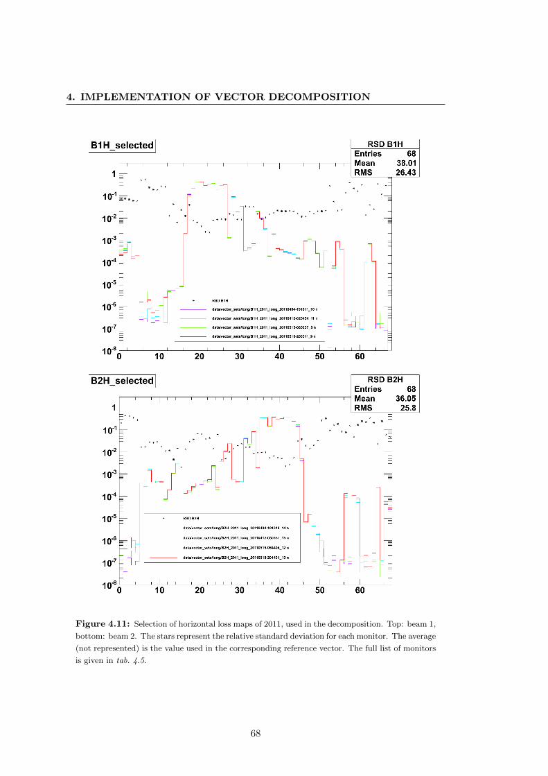
4. IMPLEMENTATION OF VECTOR DECOMPOSITION
Figure 4.11: Selection of horizontal loss maps of 2011, used in the decomposition. Top: beam 1,
bottom: beam 2. The stars represent the relative standard deviation for each monitor. The average
(not represented) is the value used in the corresponding reference vector. The full list of monitors
is given in tab. 4.5.
68

4.4 Adding more cases: longitudinal scenarios and TCTs
Figure 4.12: Selection of vertical loss maps of 2011, used in the decomposition. Top: beam 1,
bottom: beam 2. The stars represent the relative standard deviation for each monitor. The
average (not represented) is the value used in the corresponding reference vector. The full list of
monitors is given in tab. 4.5.
69
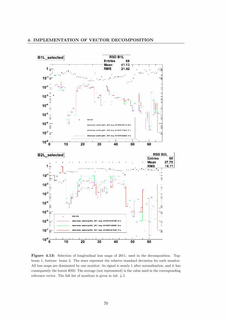
4. IMPLEMENTATION OF VECTOR DECOMPOSITION
Figure 4.13: Selection of longitudinal loss maps of 2011, used in the decomposition. Top:
beam 1, bottom: beam 2. The stars represent the relative standard deviation for each monitor.
All loss maps are dominated by one monitor: its signal is nearly 1 after normalisation, and it has
consequently the lowest RSD. The average (not represented) is the value used in the corresponding
reference vector. The full list of monitors is given in tab. 4.5.
70

4.4 Adding more cases: longitudinal scenarios and TCTs
Index BLM name Scenario
52 BLMEI.04L2.B1E10_TCTH.4L2.B1
B1H53 BLMEI.04L5.B1I10_TCTH.4L5.B1
54 BLMEI.04L8.B1E10_TCTH.4L8.B1
55 BLMEI.04L1.B1I10_TCTH.4L1.B1
56 BLMEI.04R1.B2I10_TCTH.4R1.B2
B2H57 BLMEI.04R2.B2E10_TCTH.4R2.B2
58 BLMEI.04R5.B2I10_TCTH.4R5.B2
59 BLMEI.04R8.B2E10_TCTH.4R8.B2
60 BLMEI.04L2.B1E10_TCTVB.4L2
B1V61 BLMEI.04L5.B1I10_TCTVA.4L5.B1
62 BLMEI.04L8.B1E10_TCTVB.4L8
63 BLMEI.04L1.B1I10_TCTVA.4L1.B1
64 BLMEI.04R1.B2I10_TCTVA.4R1.B2
B2H65 BLMEI.04R2.B2E10_TCTVB.4R2
66 BLMEI.04R5.B2I10_TCTVA.4R5.B2
67 BLMEI.04R8.B2E10_TCTVB.4R8
Table 4.4: List of all TCT BLMs of the LHC. The index corresponds to the BLM index in the
loss maps (cf. fig. 4.7). The TCTs are sorted by type: B1H, B2H, B1V, B2V; then by position
within one type.
Most of the monitors of IR7 give a RSD around 10−2 for the transversal loss maps.
This shows the level of reproducibility of the measures for the transversal loss maps.
Some of the highest values are explained by the fact that they correspond to mon-
itors associated to one beam, when the corresponding loss map is of the other beam.
The monitor has a low signal leading to a high RSD. However, low signals do not in-
fluence the results of the decomposition. Some of the high RSD monitors, such as the
first and last monitors of IR7, are not essential to the result of the decomposition, and
could have been removed from the selection.
All the TCTs give a worst standard deviation than the other monitors; but they
always have a signal lower than the other monitors, and thus will not influence the
decomposition.
All the longitudinal loss maps present higher RSD than the transversal ones, which
is a consequence of the different problems presented in §. 4.4.1.
71

4. IMPLEMENTATION OF VECTOR DECOMPOSITION
Index BLM name
0 BLMEI.06L3.B1I10_TCP.6L3.B1
1 BLMEI.06L3.B1I10_TCHSH.6L3.B1
2 BLMEI.06L3.B1I10_TCAPA.6L3.B1
3 BLMEI.05L3.B1I10_TCSG.5L3.B1
4 BLMEI.05L3.B1I10_TCSM.5L3.B1
5 BLMEI.05R3.B2E10_TCSM.5R3.B2
6 BLMEI.05R3.B2E10_TCSG.5R3.B2
7 BLMEI.06R3.B2E10_TCAPA.6R3.B2
8 BLMEI.06R3.B2E10_TCHSH.6R3.B2
9 BLMEI.06R3.B2E10_TCP.6R3.B2
10 BLMEI.07L7.B2I10_TCLA.A7L7.B2
11 BLMQI.06L7.B2I20_MQTL
12 BLMQI.06L7.B2I10_MQTL
13 BLMEI.06L7.B2I10_TCLA.D6L7.B2
14 BLMQI.06L7.B1E30_MQTL
15 BLMEI.06L7.B2I10_TCLA.C6L7.B2
16 BLMEI.06L7.B1E10_TCP.D6L7.B1
17 BLMEI.06L7.B1E10_TCP.C6L7.B1
18 BLMEI.06L7.B1E10_TCP.B6L7.B1
19 BLMEI.06L7.B1E10_TCP.A6L7.B1
20 BLMEI.06L7.B1E10_TCHSV.6L7.B1
21 BLMEI.06L7.B1E10_TCHSH.6L7.B1
22 BLMEI.06L7.B1E10_TCHSS.6L7.B1
23 BLMEI.06L7.B2I10_TCLA.B6L7.B2
24 BLMEI.06L7.B1E10_MBW.B6L7
25 BLMEI.06L7.B1E10_TCSM.A6L7.B1
26 BLMEI.06L7.B2I10_TCLA.A6L7.B2
27 BLMEI.05L7.B2I10_TCSM.E5L7.B2
28 BLMEI.05L7.B2I10_TCSM.A5L7.B2
29 BLMEI.04L7.B1E10_TCSG.D4L7.B1
30 BLMEI.04L7.B1E10_TCSM.D4L7.B1
31 BLMEI.04R7.B2I10_TCSM.D4R7.B2
32 BLMEI.04R7.B2I10_TCSG.D4R7.B2
33 BLMEI.05R7.B1E10_TCSM.A5R7.B1
Index BLM name
34 BLMEI.05R7.B1E10_TCSG.E5R7.B1
35 BLMEI.06R7.B1E10_TCLA.A6R7.B1
36 BLMEI.06R7.B2I10_TCSM.A6R7.B2
37 BLMEI.06R7.B2I10_MBW.B6R7
38 BLMEI.06R7.B1E10_TCLA.B6R7.B1
39 BLMEI.06R7.B2I10_TCHSS.6R7.B2
40 BLMEI.06R7.B2I10_TCHSH.6R7.B2
41 BLMEI.06R7.B2I10_TCHSV.6R7.B2
42 BLMEI.06R7.B2I10_TCP.A6R7.B2
43 BLMEI.06R7.B2I10_TCP.B6R7.B2
44 BLMEI.06R7.B2I10_TCP.C6R7.B2
45 BLMEI.06R7.B2I10_TCP.D6R7.B2
46 BLMEI.06R7.B1E10_TCLA.C6R7.B1
47 BLMQI.06R7.B2I30_MQTL
48 BLMEI.06R7.B1E10_TCLA.D6R7.B1
49 BLMQI.06R7.B1E10_MQTL
50 BLMQI.06R7.B1E20_MQTL
51 BLMEI.07R7.B1E10_TCLA.A7R7.B1
52 BLMEI.04L2.B1E10_TCTH.4L2.B1
53 BLMEI.04L5.B1I10_TCTH.4L5.B1
54 BLMEI.04L8.B1E10_TCTH.4L8.B1
55 BLMEI.04L1.B1I10_TCTH.4L1.B1
56 BLMEI.04R1.B2I10_TCTH.4R1.B2
57 BLMEI.04R2.B2E10_TCTH.4R2.B2
58 BLMEI.04R5.B2I10_TCTH.4R5.B2
59 BLMEI.04R8.B2E10_TCTH.4R8.B2
60 BLMEI.04L2.B1E10_TCTVB.4L2
61 BLMEI.04L5.B1I10_TCTVA.4L5.B1
62 BLMEI.04L8.B1E10_TCTVB.4L8
63 BLMEI.04L1.B1I10_TCTVA.4L1.B1
64 BLMEI.04R1.B2I10_TCTVA.4R1.B2
65 BLMEI.04R2.B2E10_TCTVB.4R2
66 BLMEI.04R5.B2I10_TCTVA.4R5.B2
67 BLMEI.04R8.B2E10_TCTVB.4R8
Table 4.5: List of all selected BLMs. The index corresponds to the BLM index in the loss maps
(cf. fig. 4.7). BLMs are separated by IR3, IR7, and TCTs.
72

4.5 Validation of results: Centers of Mass
Figure 4.14: All Relative Standard Deviations for each reference vector used in the decompo-
sition. The full list of monitors is given in tab. 4.5.
4.5 Validation of results: Centers of Mass
In this section, an easy way to separate between the four transversal loss scenarios will
be presented.
4.5.1 Motivation
The different algorithms return the decomposition of a given loss vector. The calculated
error tells how close a recomposition is to the original vector. It is still desirable to
have a way to find which loss scenario corresponds to a given vector without doing any
decomposition, to gain confidence in the procedure and implementation. Afterwards, it
can be applied to other loss profiles, where simple verification might be more difficult.
The choice was made to use the normalized difference between the losses at primary
collimators. It is also called Center of Mass, and for two signals a and b, is calculated as:
c =a− ba+ b
c represents the proportion of each signal: for a � b, c ' 1; for b � a, c ' −1; for
a ' b, c ' 0. For the same overall loss S ≡ a+ b, both a (for fixed b) or b (for fixed a)
73

4. IMPLEMENTATION OF VECTOR DECOMPOSITION
depend linearly of c:
c =a− bS
and b = S − a
therefore:
a =S
2· c+
S
2
for b, the result is:
b = −S2· c+
S
2
This shows that for a fixed (or normalised) total loss S, each signal depends linearly
on the center of mass if the other one is fixed: the center of mass gives the relative
proportion of the signals.
The centers of mass also have the advantage to be able to be combined: a and b
can be any combination of signals that we want to compare against each other. For
instance, a can be the sum of the signals at the vertical collimators, and b the sum of
the signals at the horizontal collimators.
4.5.2 Implementation and verifications
The values used for the centers of mass are the combinations of the signals at the four
primary collimators (cf. tab. 4.6).
Expert name Beam & plane BLM index Loss
TCP.D6L7.B1 B1 vertical 18 v1
TCP.C6L7.B1 B1 horizontal 19 h1
TCP.C6R7.B2 B2 horizontal 114 h2
TCP.D6R7.B2 B2 vertical 113 v2
Table 4.6: List of primary collimators of IP7 used in the Centers of Mass.
The centers of mass used for discrimination between beam 1 and beam 2 is:
CoM1|2 ≡(h2 + v2)− (h1 + v1)
h1 + v1 + h2 + v2(4.1)
It always varies between −1 and +1. In this case, −1 means that the measured loss
profile is made only of beam 1 scenarios, and +1 means that the measured loss profile
is made only of beam 2 scenarios. A center of mass of 0 means that both beams give
the same contribution to the overall loss.
74

4.5 Validation of results: Centers of Mass
Figure 4.15: Distributions of the results of CoM1|2 (cf. eq. 4.1). Each one of the 4 plots
corresponds to a loss scenario (known before the calculation), given in the title of each plot.
There are 7 different loss maps for each scenario (28 in total). The results of the centers of mass
match perfectly the type of every single vector. This is because the primary collimators for beam 1
are installed far away from the collimators for beam 2, and the signals at the corresponding BLMs
are well separated: on fig. 4.1, the primary collimator for beam 1 are around index 20, whereas
the ones for beam 2 are at index 116.
For horizontal and vertical cases, the center of mass is:
CoMH|V ≡(v1 + v2)− (h1 + h2)
h1 + v1 + h2 + v2(4.2)
In this case, the center of mass varies between −1 when it is dominated by signal
from the horizontal collimators and +1 when it is dominated by the signal from the
vertical collimators. Again, a center of mass of 0 shows that the losses from both planes
are equal.
In order to evaluate the correctness of the centers of mass, they were first calculated
for all 28 loss maps of 2010 (4 scenarios× 7 dates). The results are presented in fig. 4.15.
For beam discrimination, they match exactly the dominating beam (1 or 2) of every
single vector.
However, the results for the centers of mass are not as good for the separation
between horizontal and vertical loss maps (cf. fig. 4.16). They are separated, but do
75

4. IMPLEMENTATION OF VECTOR DECOMPOSITION
Figure 4.16: Distributions of the results of CoMH|V (cf. eq. 4.2). Each one of the 4 plots
corresponds to a scenario (known before the calculation), given in the title. There are 7 different
loss maps for each scenario (28 in total). The centers of mass have different values depending on
the scenarios, but they vary between −1 and −0.5, instead of varying between −1 and 1.
not give the expected results: instead of varying between −1 and 1, the results vary
between −1 and −0.5. This could be reproduced with the selected loss maps of 2011
used in the decomposition, and with all loss maps of 2011 for statistics (cf. fig. 4.17).
The CoM1|2, giving always correct results (all values are +1 or −1), are not represented.
In addition to varying in an interval smaller than expected, some of the 2011 loss
maps give a “wrong” (opposite to the expected value knowing the associated loss sce-
nario), e.g. −0.5 instead of −1 for some of the B1H loss maps of 2011 (cf. fig. 4.17,
right column, third plot down). This is not an issue: these loss maps were not selected
and are not used in the decomposition. Again, no loss map gives a CoMH|V bigger
than zero.
This is due to the relative position of the corresponding collimators: the horizon-
tal collimators sits downstream and next to the vertical one. The secondary shower
produced when the protons hit the vertical collimator will also be detected by the hor-
izontal collimator: part of the signal seen by the horizontal collimator comes from the
vertical one.
76
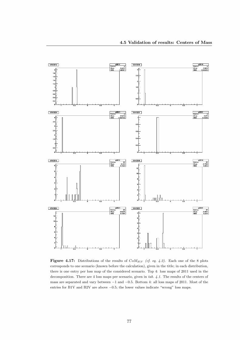
4.5 Validation of results: Centers of Mass
Figure 4.17: Distributions of the results of CoMH|V (cf. eq. 4.2). Each one of the 8 plots
corresponds to one scenario (known before the calculation), given in the title; in each distribution,
there is one entry per loss map of the considered scenario. Top 4: loss maps of 2011 used in the
decomposition. There are 4 loss maps per scenario, given in tab. 4.1. The results of the centers of
mass are separated and vary between −1 and −0.5. Bottom 4: all loss maps of 2011. Most of the
entries for B1V and B2V are above −0.5; the lower values indicate “wrong” loss maps.
77
4. IMPLEMENTATION OF VECTOR DECOMPOSITION
Several corrections were considered, such as subtracting the signal of the vertical
collimator from the horizontal one, or stretching the variation interval.
Implementing the first method showed that a factor of roughly two times the vertical
signal had to be subtracted in order to get a correct variation interval; but this created
a pole for the function (h, v) 7→ (h − α · v, v), i.e. a value for which the function
would diverge to infinity. Arbitrarily stretching the variation interval, corresponding to
the precedent method with no pole and a correction factor of higher value, led to the
problem of some values of the centers of mass being higher than one, in cases where
the cross-talk between the two monitors is overestimated.
Eventually, the choice was made to keep the centers of mass uncorrected, knowing
that the horizontal/vertical one would vary between −1 and −0.5.
4.6 Choice of the algorithm
In this section, the reasons to use or not the different decomposition algorithms will be
discussed.
SVD
The Singular Value Decomposition has the drawback of sometimes returning negative
factors, which have no physical meaning. However, it is the algorithm which gives the
results closest to the original vector in the sense of the norm of the difference vector:
the difference was calculated to be of the order of 10−16 to 10−18 for simple examples
with 3× 4 matrices. The choice was made to keep this decomposition technique, even
if some results are not physical.
MICADO
The implementation and the first results of MICADO showed that the results are
extremely close to the results of the Singular Value Decomposition: the difference
is of the order of 10−16 to 10−18. Both SVD and Micado give the closest possible
recomposition. The choice was made to use only the SVD.
78

4.7 Evaluation of the correctness of a decomposition
Gram-Schmidt
The Gram-Schmidt decomposition returns mainly one vector, and is then not as close
to the original vector (in the sense of the norm of the difference). However, the results
are always physical. The choice was made to keep this decomposition technique as well.
4.7 Evaluation of the correctness of a decomposition
4.7.1 Correct and incorrect decompositions
Several verifications were made in order to evaluate the quality of each loss map. It
allowed to get some statistics on the results of the different algorithms. Additionally,
one extra vector was decomposed on each set: it is a way to cross-check the loss maps
using a common reference. Every time, the error between the chosen vector and its
recomposition was calculated, allowing the comparison between sets of loss maps.
Then, every loss map of every set was decomposed on all the other sets. This way,
loss maps giving bad results — that is, leading to wrong decompositions on every other
vector set — could be removed.
The error on the recomposition, presented in § 3.5, evaluates the difference be-
tween a vector and its recomposition in the m-vector space, but gives no information
on how correct the decomposition is. For a vector corresponding to a known scenario,
an incorrect decomposition (wrong linear combination of vectors) could produce a re-
composition closer to the vector than the correct one.
The point of this section is to try to show a link between the value of the error on
the recomposition and the correctness of this recomposition. It could for instance be
expressed as a threshold value of the error, below which the decomposition is considered
as correct.
4.7.2 Method and results
Different series of cross-checks were done: all the loss maps were decomposed on dif-
ferent vector sets, and the errors on the recompositions were calculated. The scenario
associated to the loss maps being of course known, the decomposition could be sorted
as correct or incorrect. In case of factors bigger than one (SVD), the decomposition
was considered as correct if the highest factor was the correct one.
79

4. IMPLEMENTATION OF VECTOR DECOMPOSITION
Figure 4.18: Distributions of correct (left) and incorrect (right) decompositions for G-S (top)
and SVD (bottom) of every loss map of 2010 on every vector set (of the same loss maps). There
are 120 decompositions in total. The averages are lower for the SVD (better recompositon), and
the correct and incorrect are close to each other. See text for more observations.
Then, the distributions of the errors for correct and incorrect decompositions were
ploted, and their averages calculated. The more separated these two averages are, the
better the discrimination between correct and incorrect decompositions will be.
The first cross-checks were done with the loss maps of 2010 (cf. tab. 4.1), both for
SVD and G-S. Every loss map of each vector set is decomposed on all the other vector
sets: there are 120 decompositions in total. The results are presented in fig. 4.18. The
averages for correct and incorrect are, for G-S : 0.2105 and 0.2188; for SVD: 0.1631
and 0.1845. They are too close to each other to allow a good separation; there is an
important overlaps between the two distributions.
Another observation is that every distribution is separated into two groups: many
values are under 0.15, corresponding to true positives for the correct decompositions,
but fake positives for the incorrect ones: the recomposition is incorrect, but close to
the original vector. Similarly, a group of values seems to be centered around 0.45,
especially for the correct GS decompositions. There are true negatives for the incorrect
SVD decompositions. The similar values, for the correct decompositions, are fake
80

4.7 Evaluation of the correctness of a decomposition
Figure 4.19: Distributions of correct (left) and incorrect (right) decompositions for G-S (top)
and SVD (bottom) of every loss map of 2010 on the average vector set. There are 24 decompositions
in total. The averages are lower for the SVD (better recomposition), and the correct and incorrect
are still too close to each other to allow a good separation. See text for more observations.
positives: far from the original vector, yet correct.
A second cross-check was done by decomposing every loss map of 2010 on the
average vector set (only for H and V): 24 decomposition in total (cf. fig. 4.19). The
first observation is that there are more correct decompositions than incorrect. However,
there is still some overlaps, and the averages are still too close to each other to allow
a good separation (0.1885 and 0.2186 for G-S; 0.1691 and 0.2124 for SVD). This is
because the loss maps of 2010 were not sorted like the 2011 ones, following the order
in which they were measured and the energy. The importance of these differences was
only understood later.
4.7.3 Distributions of the error for the 2011 loss maps
In this case, all loss maps of 2011 were decomposed on the average set of selected
loss maps (cf. § 4.3), which is the set used in real data decompositions. In these, the
majority of correct and incorrect decompositions are clearly separated.
81

4. IMPLEMENTATION OF VECTOR DECOMPOSITION
Figure 4.20: Distributions of correct (left) and incorrect (right) decompositions for G-S (top)
and SVD (bottom) of every loss map of 2011 on the set of selected loss maps. There are 104
decompositions in total. The red lines represent the value of the geometrical mean between the
means for correct and incorrect decompositions (see text). The majority of correct and incor-
rect decompositions are now clearly separated, even though there is still some fake negatives:
distributions that are correct but far away from the original vector, and some fake positives.
For SVD, the averages for the correct decomposition is 0.1289 and 0.2732 for in-
correct (cf. fig. 4.20). The arithmetic mean between these two values is 0.201, and the
geometric mean is 0.187 (the geometric mean is often preferred here, because it takes
better into account the fact that there are many low values). Using 0.19 as a threshold,
there are 51 entries below this value for the correct decomposition, corresponding to
72% true positives; and 20 entries above mean represent 28% fake negatives. For the
incorrect decompositions, there are 26 entries above mean (79% true negative) and 7
below (21% fake positives).
For GS, the “correct” average is 0.1935, and the “incorrect” is 0.2881. The arith-
metic mean between them is 0.236, and the geometric mean is 0.241 (there is no dif-
ference between arithmetic and geometric mean at the precision of 0.01 used in the
distribution). For the correct decompositions, there are 38 entries below mean (54%
true positives) and 33 above (46% fake negatives); for the incorrect decompositions, 24
above (73% true negatives) and 9 below (27% fake positives).
82

4.8 Application to LHC data
4.7.4 Conclusion on the values of the error
From these observations (especially on the distributions for 2011, which were selected
much more carefully than the ones from 2010, keeping only the ones measured first),
it appears than using only one value as a threshold would not separate correct and
incorrect decompositions clearly. Considering different “cuts” would lead to a better
separation into three categories. All errors below 0.1 are assumed to be correct decom-
positions; between 0.1 and 0.3, the result is undefined; and above 0.3, the decomposition
is considered as wrong. This suppresses nearly all fake positives, but still leaves some
fake negatives.
4.8 Application to LHC data
This section will present how the different decompositions are applied to LHC data,
by opposition to the specific loss maps that were used for cross-checks, and the choices
that were made. The results will be presented in chapter 6.
4.8.1 Implementation
After trials and cross-checks on different loss maps, the decompositions were calculated
during physics beams of 2011. More specifically, the periods during which “stable
beams” had been declared: most of the beam characteristics are left unchanged, and
physics collisions are measured in the experiments.
Losses are studied at each second; the ensemble of losses at one second is called
current loss profile. This specific frequency corresponds to the frequency at which data
are recorded in the measurement database (cf. §. A.2.3). In addition, a default loss
profile corresponding to the average loss in nominal condition was created.
Beam losses are by definition not very high during stable beams: the losses are
considered safe and are lower than the loss thresholds. If they get bigger, they lead to a
“beam dump”, and this case is not considered here; and the high losses not leading to
a beam dump are rare. Consequently, a few non-stable beam periods were also studied,
especially the LHC modes preceding stable beams periods, such as injection, ramp,
squeeze and adjust.
83

4. IMPLEMENTATION OF VECTOR DECOMPOSITION
4.8.2 Evolution of losses
The first check to do on the losses is to evaluate the evolution of the losses from one
second to the other: that is, the “difference” between the loss profile at the current
second and the loss profile at the previous second. Both loss profiles are considered as
vectors with all ionisation chambers in LHC (NBLM coordinates).
Several techniques can be used here, showing different aspects of the evolution of
losses: the euclidean norm of the difference between the two vectors; the euclidean norm
of the vector itself; the scalar product of the two vectors; the sum of all coordinates.
Euclidean norm of the difference
The first value calculated here is the norm of the difference (subtraction) between
the normalised vector representing the losses at one second and the normalised vector
representing the losses at the previous second (cf. fig. 4.21):∥∥∥∥∥ ~X(t+ 1)
‖ ~X(t+ 1)‖−
~X(t)
‖ ~X(t)‖
∥∥∥∥∥ (4.3)
Both vectors are normalized before calculating the subtraction: thus, this value
depends only on the shape of the two vectors. As an illustration, let’s consider the case
where losses appear in one part of the LHC at one second; then, at the next second,
losses of the exact same intensity (normalisation) appear in a different part of the LHC.
Even if the norm of the corresponding vectors is the same for both seconds, the norm
of the difference will give a high result. It is sensitive to changes of shape even if the
norms of both vectors are strictly equal, which is the case after normalisation.
Norm of the vector
Calculating the euclidean norm of the vector is a good way to evaluate the magnitude
of the overall losses in the LHC (cf. fig. 4.21). It is the standard norm on a vector
space. It is written:
|| ~X|| =√∑
i
x2i (4.4)
where the (xi) are the coordinates of the vector ~X.
84
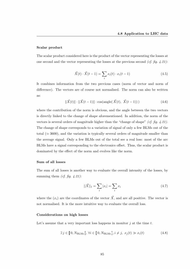
4.8 Application to LHC data
Scalar product
The scalar product considered here is the product of the vector representing the losses at
one second and the vector representing the losses at the previous second (cf. fig. 4.21):
~X(t) · ~X(t− 1) =∑i
xi(t) · xi(t− 1) (4.5)
It combines information from the two previous cases (norm of vector and norm of
difference). The vectors are of course not normalised. The norm can also be written
as:
‖ ~X(t)‖ · ‖ ~X(t− 1)‖ · cos(angle( ~X(t), ~X(t− 1)) ) (4.6)
where the contribution of the norm is obvious, and the angle between the two vectors
is directly linked to the change of shape aforementioned. In addition, the norm of the
vectors is several orders of magnitude higher than the “change of shape” (cf. fig. 4.21).
The change of shape corresponds to a variation of signal of only a few BLMs out of the
total (' 3600), and the variation is typically several orders of magnitude smaller than
the average signal. Only a few BLMs out of the total see a real loss: most of the arc
BLMs have a signal corresponding to the electronics offset. Thus, the scalar product is
dominated by the effect of the norm and evolves like the norm.
Sum of all losses
The sum of all losses is another way to evaluate the overall intensity of the losses, by
summing them (cf. fig. 4.21):
|| ~X||1 =∑i
|xi| =∑i
xi (4.7)
where the (xi) are the coordinates of the vector ~X, and are all positive. The vector is
not normalised. It is the more intuitive way to evaluate the overall loss.
Considerations on high losses
Let’s assume that a very important loss happens in monitor j at the time t.
∃ j ∈ [ 0, NBLMs ], ∀i ∈ [ 0, NBLMs ], i 6= j, xj(t)� xi(t) (4.8)
85

4. IMPLEMENTATION OF VECTOR DECOMPOSITION
Figure 4.21: Top: values of the Euclidean norm of the current loss profile (purple), the scalar
product of two consecutive loss profiles (green), the sum of all losses in the current loss profile (red).
Bottom: values of the euclidean norm of the difference between two consecutive loss profiles. Note
that the three top plots are very similar: they show similar information. The norm of difference
displays a different information, but still relates to the others: the highest values appear at the
same time.
86

4.8 Application to LHC data
where the (xi) are the coordinates of the vector ~X. This assumption is not realistic for
only one monitor; however, it is for valid for the sum of the signals of a few monitors
(such as the ones around a primary collimator in IR7). It has been observed in the
LHC, where their losses can be several orders of magnitude higher than the default loss
level. For simplicity, the equations will be written with only one xj :
xj(t) + xi(t) ∼ xj(t)
We want to assume that the high loss xj is higher than the sum of all losses in the
LHC:
xj(t)�∑i 6=j
xi(t) (4.9)
This requires that the high loss is at least four orders of magnitude higher than the
default loss level, because there are 3600 monitors considered here. Assuming that all
(xi) for i 6= j have roughly the same value, the default (low) loss level, xj needs to
satisfy:
xj(t)� 3600× xi(t)
Again, this assumption is not realistic for one monitor (this situation happens only
rarely). However, the same observation could be done for several monitors recording
high losses satisfying eq. 4.8; in this case, their sum will satisfy the previous equation.
For simplicity, the equations will be written with only one xj . We can then write:
(4.9) ⇒ xj(t) +∑i 6=j
xi(t) ∼ xj(t) ⇒∑i
xi ' xj ⇒ ‖ ~X‖1 ' xj (4.10)
This corresponds to the intuitive idea that all losses are smaller than and negligible
compared to the loss in monitor j, and also that the sum of all losses for i 6= j is smaller
than and dominated by the loss in monitor j.
The equivalent arguments can be applied to the euclidean norm; at first order:
(4.8) ⇒ x2j (t) +
∑i 6=j
x2i (t) ' x2
j (t) ⇒∑i
x2i (t) ' x2
j (t)
⇒ ‖ ~X(t)‖ ' xj(t) (4.11)
87

4. IMPLEMENTATION OF VECTOR DECOMPOSITION
For the scalar product, we need to introduce a second vector. Let’s consider a vector
~X(t+ 1) that is assumed to be nominal. All losses at the time t+ 1 will be negligible
compared to the loss in monitor j at the time t:
∀i ∈ [ 0, NBLMs ], xi(t+ 1)� xj(t) (4.12)
Especially: xj(t+ 1)� xj(t).
The scalar product considered here is expressed as:
~X(t) · ~X(t+ 1) =∑i
xi(t)× xi(t+ 1)
Multiplying both sides of eq. 4.8 by xi(t+ 1) gives:
xj(t)× xi(t+ 1)� xi(t)× xi(t+ 1)
and this is true for all xi(t+ 1), including xj(t+ 1). Thus:
xj(t)× xj(t+ 1)� xi(t)× xi(t+ 1)
With the same assumption as in eq. 4.9 (the sum of all 3600 losses for i 6= j is
dominated by the loss in monitor j), we get:
xj(t)× xj(t+ 1)�∑i 6=j
xi(t)× xi(t+ 1)
⇒ ~X(t) · ~X(t+ 1) ' xj(t)× xj(t+ 1)
~x(t) · ~x(t+ 1) ∝ xj(t) (4.13)
The results (4.10), (4.11) and (4.13) (the proportionality factor being different in
each case) show that in case of a high loss, the norm, the sum of all losses and the
scalar product will all behave similarly (cf. fig. 4.21 top).
This conclusion can be broadened by considering, instead of the monitor #j, the
k highest monitors dominating the others. This corresponds to the idea that the dis-
tribution of signals is not uniform: there are a lot of monitors with low signal (around
offset), several monitors with high signals (orders of magnitude above offset) and very
few in between. The euclidean norm, the sum of all losses and the scalar product all
behave like the k dominating monitors. This is visible in fig. 4.21.
88

4.8 Application to LHC data
4.8.3 Default Loss Profile
Another point of going through the losses in the LHC every second is to calculate a
Default Loss Profile for the stable beams in the LHC. It is achieved by taking the
average of the losses of each monitors during several stable beams periods. It can be
done with a 2D histogram, showing the distribution of signal on one dimension, all
monitors being displayed on the other dimension. It is then easy to extract the mean
and standard deviation for each monitor.
After that, the variation between the current loss profile and the default loss profile
can be calculated at each second. It will be presented in the next chapter.
89

4. IMPLEMENTATION OF VECTOR DECOMPOSITION
90

Chapter 5
Time evolution of the beam loss
in the LHC
The work presented in this chapter concentrated on studying the time evolution of the
Beam Loss Monitors signals during nominal operation. These losses are considered as
a vector, as presented in chap. 4, but this time all monitors are considered together.
The point is to learn how the losses evolve; check where important losses occur, and
which parts of the LHC are free from losses. It will also give a better understanding of
the behaviour of the vectors, and what information can be extracted from their time
evolution.
5.1 Default Loss Profile
5.1.1 Interest
The default loss profile can be used to evaluate how much the current loss profile differs
from normal. It is the average loss measured in each monitors. It is purely empiric and
comes only from measurements: all the losses of all the BLMs in the LHC were recorded
for all seconds of several stable beam periods of the running of the machine. The “stable
beam” flag in the LHC indicates that the machine has reached its maximum energy
(3.5 TeV at the time), that the beams are colliding, and that none of the main settings
of the machine (energy and β*, the value of the beta function at the interaction point)
will be changed.
91
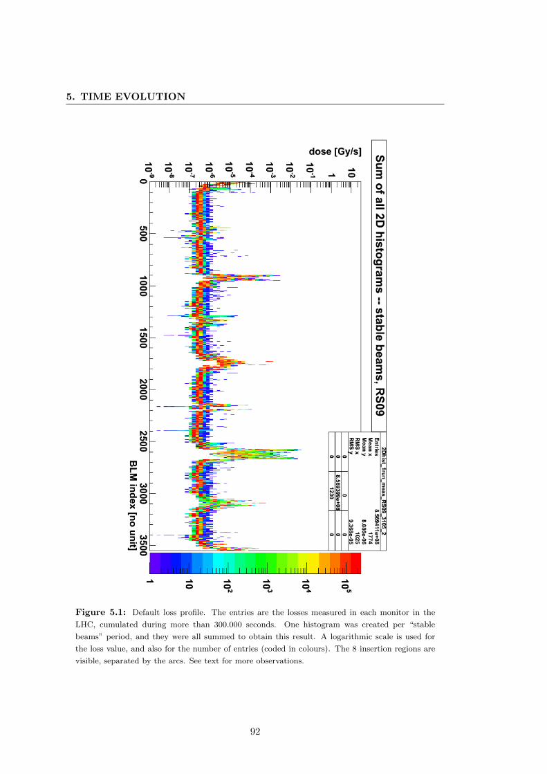
5. TIME EVOLUTION
Figure 5.1: Default loss profile. The entries are the losses measured in each monitor in the
LHC, cumulated during more than 300.000 seconds. One histogram was created per “stable
beams” period, and they were all summed to obtain this result. A logarithmic scale is used for
the loss value, and also for the number of entries (coded in colours). The 8 insertion regions are
visible, separated by the arcs. See text for more observations.
92

5.1 Default Loss Profile
The default loss profile is not normalised: the real value of the average loss in each
monitor is kept, in order to give a good overview of what the nominal losses are in
the LHC. These signal distributions show which monitors record a near constant signal
(most entries in the same bin), and where the intensity of the loss for one monitor
varies even during stable beams (entries spread over several bins).
5.1.2 Creation
The losses are gathered in a two dimensional histogram. The horizontal axis corre-
sponds to the index of the BLM sorted by position (DCUM). The vertical axis gives
the value of the integrated dose: the loss, in Gy/s. The dynamic range of the BLMs
for running sum 9 — from 10−9 Gy/s to 23.7 Gy/s — was divided following an expo-
nential scale. The bin height is constant in logarithmic scale. Every second, one entry
per monitor is added. The result is that each “column” corresponds to the 1-dimension
logarithmic distribution of the signal in this BLM, for all the hours of measurement
(cf. fig. 5.1).
5.1.3 Observations
Several observations show that the presented default loss profile described accurately
the “default loss” in the LHC; and show that further processing would not modify the
profile.
� Most BLMs have the majority of their signals within one bin: ∼ 2 ·105 entries out
of the ∼ 2.45 · 105 total entries per monitor are within the same bin. This shows
how constant the loss is: the standard deviation is smaller than the average value
(cf. § 5.2.1).
� For arc monitors, no signal significantly above the electronics offset (10 pA,
cf. § 2.3) was recorded for the whole period of measurement. The value of this
offset for RS09 corresponds to 1.8 · 10−7 Gy/s; most of the entries are between
2 Gy/s and 4 Gy/s. This is the value of the offset in the arcs and the fluctuations
of the signal measured when there is no beam in the machine, just above the
electronics offset.
93

5. TIME EVOLUTION
� The only higher signals (the isolated purple bins) always correspond to only 1
event. This means that, within the precision of the BLM system (if there were
real losses, they were lower than the noise), and taking into account the offset of
the electronics, there was no real loss recorded.
� The BLMs that show more fluctuation are situated at the 8 interaction regions,
where the optics is different from the rest of the ring, where all collimators and
absorbers are installed, and where luminosity induced losses can appear. All
noticeable losses (above noise level) happen in very few specific places in the
LHC; the losses only appear where they should.
� These monitors, recording high losses, do not show any signal at the offset level
(level of the arc monitors), as they would if there was no beam in the machine.
This means that the level of loss observed there is constant. All recorded signals
correspond to particle lost during operation; if signals had been recorded when
there is no beam in the machine, these monitors would show signal at the level
of the offset (like the arc monitors).
� A few monitors corresponding to the neutral beam absorbers (TANs) at IR1 and
IR5 have most of their signal in a very high bin (e.g. isolated red bin around index
20 and 1700). This is due to the luminosity induced losses, the debris (protons of
lower energy and other particles produced during collision). The level of debris
and the luminosity were approximatively constant during the time of study.
5.1.4 Comparisons of the loss in the LHC with the default loss profile
Once the average loss value of each BLM during “stable beams” was extracted from
the histogram, comparisons were done between the current loss profile and the default
loss profile, using the same techniques as for the comparison with the previous second
(cf. § 4.8.2): that is, scalar product (cf. fig. 5.2, bottom left) and norm of the difference
(cf. fig. 5.2, bottom right).
In this case, the scalar product gives a result similar in shape to the euclidean norm√∑x2i and the sum of all losses
∑|xi| (cf. fig. 5.2). Reasons for this were discussed
in § 4.8.2. The correlation between the scalar product of the loss vector at one second
94
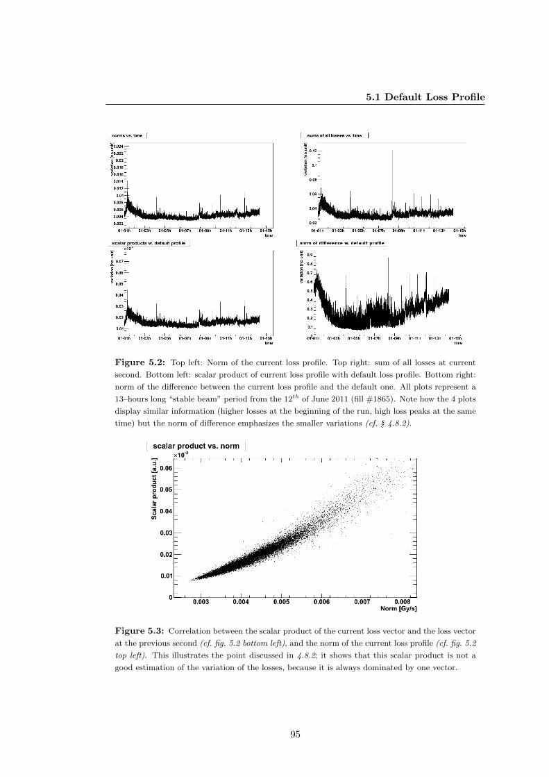
5.1 Default Loss Profile
Figure 5.2: Top left: Norm of the current loss profile. Top right: sum of all losses at current
second. Bottom left: scalar product of current loss profile with default loss profile. Bottom right:
norm of the difference between the current loss profile and the default one. All plots represent a
13–hours long “stable beam” period from the 12th of June 2011 (fill #1865). Note how the 4 plots
display similar information (higher losses at the beginning of the run, high loss peaks at the same
time) but the norm of difference emphasizes the smaller variations (cf. § 4.8.2).
Figure 5.3: Correlation between the scalar product of the current loss vector and the loss vector
at the previous second (cf. fig. 5.2 bottom left), and the norm of the current loss profile (cf. fig. 5.2
top left). This illustrates the point discussed in 4.8.2; it shows that this scalar product is not a
good estimation of the variation of the losses, because it is always dominated by one vector.
95

5. TIME EVOLUTION
and the loss vector at the previous second, and the norm of the loss vector, is shown
in fig. 5.2.
The scalar product of the loss vector at a time x(t) with the default loss profile y
is written:
~x(t) · ~y =∑i
xi(t) · yi
where xi(t) is the loss measured by the monitor i at t and yi is the calculated average
loss for this monitor.
Every second, the loss xi(t) is multiplied by a constant yi: the scalar product with
the default profile can be seen as a strictly monotonic (increasing) application. It will
describe the overall loss in a similar way to the norm of the loss vector.
The norm of the difference is:
|~x(t)− ~y| =√∑
i
(xi(t)− yi)2
As shown in § 3.5 and § 4.8.2, this value is better than the others to quantify the
relative variations of two vectors close to each other.
Some effects were observed on all stable beam runs which were investigated. Even
when the beams are declared “stable”, the current loss profile is different from the
default loss profile: the subtraction is never equal to zero (cf. fig. 5.2). The current
profile gets closer to the default profile (the norm of the difference decreases), and after
about two hours, it is at the closest to the default profile (minimum of the difference).
Then, several hours later, the difference starts increasing again. The current loss profile
gets more and more different from the default one.
5.2 Individual evolution of the signal of a BLM
In this section, we will study the evolution of the signal of one monitor considered
independently, for different types of monitors.
5.2.1 Arc monitor — low signal
The distributions of all losses (cf. § 5.1.2 and fig. 5.1) showed that the monitors from the
arc have an extremely narrow distribution, with a standard deviation of ∼ 2 ·10−8 Gy/s
96

5.2 Individual evolution of the signal of a BLM
Figure 5.4: Top: Distributions of the signal of arbitrary arc monitors, from the 8 arcs of
the LHC, for RS09. This figure shows how similar the distributions are, in shape and value,
even for monitors situated far away from each other. The 10 pA electronics offset corresponds to
1.8 ·10−7 Gy/s, which is within the variations of signal. The BLMs see no loss. Bottom: Separated
distributions of the signal of arbitrary arc monitors. These figures give the values of average signal
and standard deviation.
97

5. TIME EVOLUTION
(compared to the dynamic range of 108) for roughly 300.000 entries. The signal of these
monitors was studied in detail.
The BLMs were arbitrarily selected and taken from the 24th cell on the left of each
interaction point, which is far away from the interaction points. The figure 5.4 top
shows that the distributions are similar in shape and in value. Most arc monitors behave
the same way, and the selected ones are a representative sample as seen in fig. 5.1.
All the values of average and standard deviation of the different signal distributions,
calculated numerically, are given by fig. 5.4 bottom: average is around 2.3 · 10−7 Gy/s,
and standard deviation around 1.8 · 10−8 Gy/s for running sum 9.
The values of the average signal are very close to the value of the 10 pA current
offset permanently sent in the tunnel electronics. It corresponds roughly to a value of
65 expressed in bit units, and 1.8 ·10−7 Gy/s for running sum 9. The smallest step, one
bit unit, is worth 2.76 · 10−9 Gy/s.
Moreover, the signal of these monitors was checked during times when there was
no beam in the machine, and the signal distributions showed the same average. This
shows that the arc monitors record no signal coming from deposited charges, and the
signal measured over the offset level is only due to noise. There are no detectable losses
in the arcs during normal operation.
5.2.2 Variations of the signal of a monitor
After studying the distribution of the low-signal BLMs, the next step was to study the
variations of these signals. It was done by calculating the distribution of the difference
between the signal of one BLM at one second and the previous second (cf. fig. 5.6).
This allows to study the effect of the noise.
The first observation is that the distribution of variation is similar for all chosen
monitors, and has an mean value of zero at the precision of the measurement of the
loss: the size of one bin corresponds to the value of one electronics bit. Then, the
distribution can be fitted with a Gaussian (cf. fig. 5.5). The values of the mean and
standard deviation given by the fit agree with the numerical average and standard
deviation of the distributions (cf. fig. 5.6) to a precision higher than one electronics
bit. The quality of the fit, including the errors, is given by the value of χ2 over the
number of degrees of freedom, and was calculated to be ' 0.82.
98

5.2 Individual evolution of the signal of a BLM
Figure 5.5: Example of a Gaussian fit of the distribution of the signal variation of an arc
monitor. The values of the σ and µ parameters of the gaussian agree with the numerical average
and standard deviation to a precision higher than one electronics bit (width of one histogram bin).
To the level of precision of the loss measurement, the variations of the signal are
Gaussian.
BLM expert name Location
BLMEI.04R1.B1E10_TANAR.4R1 Right of IR1
BLMEI.04R1.B2I10_TCTVA.4R1.B2 Right of IR1
BLMEI.04R7.B1E10_TCSG.A4R7.B1 Right of IR7
BLMEI.03L5.B1I10_MQXA Left of IR5
BLMEI.03R1.B1E30_MQXA Right of IR1
BLMEI.04R7.B2I30_MQWA.A4R7 Right of IR7
Table 5.1: Lists of monitors showing a high average signal (around 10−4 Gy/s) in the default
loss profile. The names are given in the same order as in fig. 5.7 top.
5.2.3 IP monitors — high signal
The same study was done for monitors showing a permanently high signal (cf. fig. 5.7).
BLMs having some of the highest average signals (around 10−4 Gy/s) were selected.
99
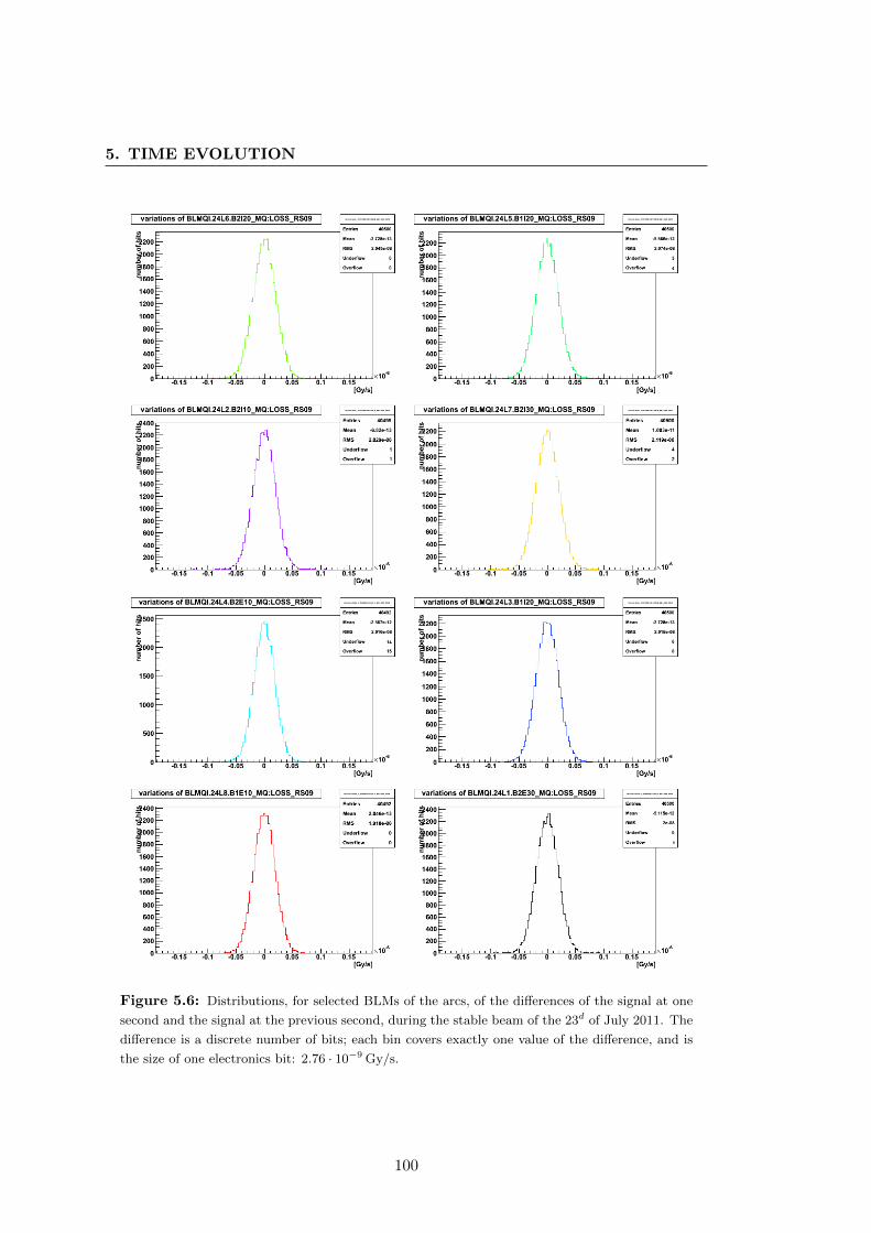
5. TIME EVOLUTION
Figure 5.6: Distributions, for selected BLMs of the arcs, of the differences of the signal at one
second and the signal at the previous second, during the stable beam of the 23d of July 2011. The
difference is a discrete number of bits; each bin covers exactly one value of the difference, and is
the size of one electronics bit: 2.76 · 10−9 Gy/s.
100
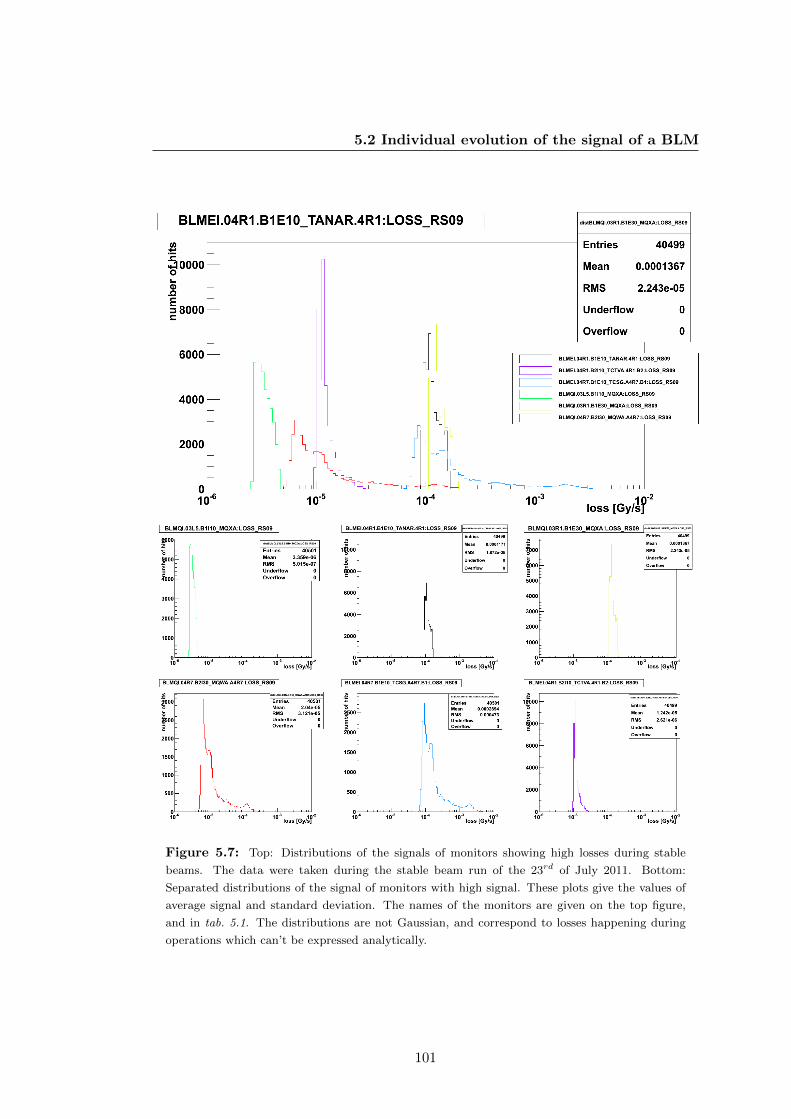
5.2 Individual evolution of the signal of a BLM
Figure 5.7: Top: Distributions of the signals of monitors showing high losses during stable
beams. The data were taken during the stable beam run of the 23rd of July 2011. Bottom:
Separated distributions of the signal of monitors with high signal. These plots give the values of
average signal and standard deviation. The names of the monitors are given on the top figure,
and in tab. 5.1. The distributions are not Gaussian, and correspond to losses happening during
operations which can’t be expressed analytically.
101
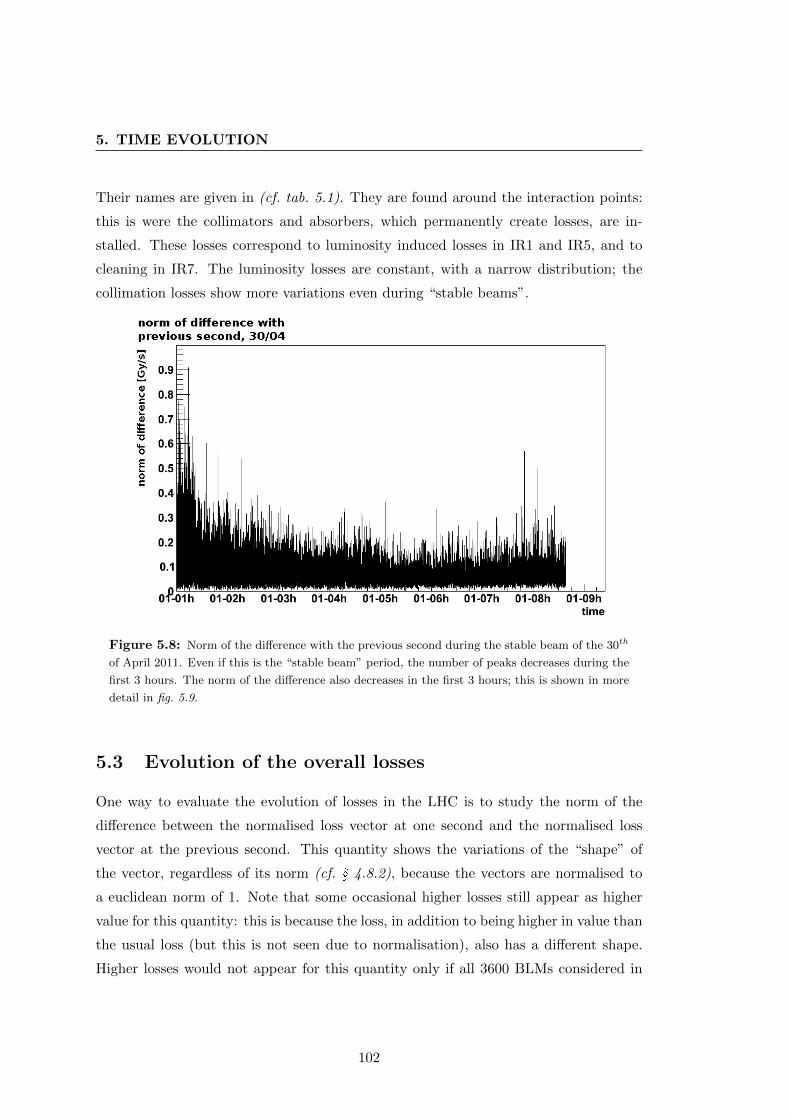
5. TIME EVOLUTION
Their names are given in (cf. tab. 5.1). They are found around the interaction points:
this is were the collimators and absorbers, which permanently create losses, are in-
stalled. These losses correspond to luminosity induced losses in IR1 and IR5, and to
cleaning in IR7. The luminosity losses are constant, with a narrow distribution; the
collimation losses show more variations even during “stable beams”.
Figure 5.8: Norm of the difference with the previous second during the stable beam of the 30th
of April 2011. Even if this is the “stable beam” period, the number of peaks decreases during the
first 3 hours. The norm of the difference also decreases in the first 3 hours; this is shown in more
detail in fig. 5.9.
5.3 Evolution of the overall losses
One way to evaluate the evolution of losses in the LHC is to study the norm of the
difference between the normalised loss vector at one second and the normalised loss
vector at the previous second. This quantity shows the variations of the “shape” of
the vector, regardless of its norm (cf. § 4.8.2), because the vectors are normalised to
a euclidean norm of 1. Note that some occasional higher losses still appear as higher
value for this quantity: this is because the loss, in addition to being higher in value than
the usual loss (but this is not seen due to normalisation), also has a different shape.
Higher losses would not appear for this quantity only if all 3600 BLMs considered in
102

5.3 Evolution of the overall losses
Figure 5.9: Distributions of “time slices” of the norm of the difference between the normalised
current loss vector and the normalised loss vector at the previous second. Each histogram has one
entry per second, and corresponds to one hour of stable beam except the last one (red) because
the beam was dumped. The distributions have less high values and get narrower with time. The
X axis is the value of the norm of the difference, and the Y axis is the number of entries per bin.
The values of mean and standard deviation are valid in spite of the overflow, because they are
calculated numerically with the real value even if it is higher than the maximum bin.
103

5. TIME EVOLUTION
the LHC would see their signal multiplied by the same unique value from one second
to another. This is of course unlikely.
All the studied “stable beam” runs showed that this value decreases in the first hours
of the run, and that peaks happening during these first hours then tend to decrease
(cf. fig. 5.8). This means that the losses in the LHC are more subject to variations
during the first hours of the “stable beam”.
In order to show this more precisely, the distributions of the norm of the difference
along time were calculated (cf. fig. 5.9). The higher values happen when the shape of
the loss vector is different from one second to another; the low values happen when
the shape of the loss vector at one second is similar to the one at the previous second.
Fig. 5.9 shows that the number of high values decreases with time. The distributions get
narrower, with less high values (important changes of shape) and more values around
average. The mean value of the distribution, around 0.06, is the average variation of
shape of the normalised loss vector.
5.4 Conclusion
In this chapter, several points were validated: a default loss profile could be extracted,
and the fact that nearly no losses happen in the arcs (only rare occasional ones) was
ascertained. Consequently, the fact that some monitors have a “constant” loss level
(standard deviation which is two orders of magnitude lower than their average signal)
means that any loss above this level carries the information that non-nominal events
happened. No decomposition is therefore needed.
The choices of the losses in IR7 and IR3 as the base for the study were validated by
the fact that they are the places in the LHC where the losses have the widest spread;
thus, were information can be extracted.
104

Chapter 6
Spatial distribution and
decomposition of the beam loss
In this chapter, the results of the vector decomposition applied to the nominal running
conditions will be presented, for vector bases from 2011. These results will be associated
to other beam measurements. The way the decomposition is calculated is explained in
the previous chapters.
6.1 Results of decomposition
In this section, the results of the decomposition will be presented, as well as the way
to display them.
6.1.1 Presentation of the results
For each second of stable beam, the loss vector was created (offset subtracted, nor-
malised) and decomposed using the SVD and Gram-Schmidt algorithms. For each
second, the factors of the decomposition are calculated: one factor per vector. In ad-
dition, the factors are used to recompose the vector, and the recomposition error (as
described in § 3.5) is calculated: the norm of the difference between the recomposed
vector and the current loss vector (both normalised).
For each second, the value of the centers of mass (cf. § 4.5) is also calculated. The
goal is to give a simple result on the type of loss at the current second, and to allow a
comparison.
105

6. SPATIAL DECOMPOSITION
6.1.2 Displaying the decomposition
Decomposition vs. time
One way to display the decomposition factors is to plot them versus time. Several of
these decompositions will be presented in § 6.2. It allows to show how the decomposition
evolves with time, and which loss scenario is dominating at each second. Similarly, the
factors associated with the tertiary collimators are represented versus time (cf. fig. 6.4).
In addition, the decomposition error is displayed, in order to evaluate the accuracy
of the decomposition (cf. § 4.7): it evaluates the difference (norm of the subtraction
vector) between the original vector and its recomposition using the given factors.
For the centers of mass, the two different aspects (vertical / horizontal, beam 1 /
beam 2) are separated (cf. § 4.5, eq. 4.1, eq. 4.2). The values of the centers of mass vary
between -1 and -0.5 for H/V; between -1 and 1 for B1/B2. Since they are numerical,
and are not the product of a decomposition, no decomposition error can be calculated
on these values; however, the results have to be interpreted carefully (cf. § 4.5). The
measurement errors are on the signal of the BLMs.
2-dimensional representation
The two aspects considered here (the transverse planes and the beams) can be put on
two different axes. This way, the relative composition of the loss at a time is displayed
with one point.
For the centers of mass, the coordinates of a point at one time t are (CoM1|2(t),
CoMH|V (t)). The time is coded by colour: it starts with purple, and goes to blue,
green, yellow and finally red (cf. fig. 6.1). This type of display can be useful for a real
time calculation and display of the centers of mass. The position of the point includes
all the information on the centers of mass.
The same type of display is not as direct for the result of the decomposition because
there are as many factors (fi) as the number of vectors. The four transversal factors
could be combined in different ways, such as a Center of Mass, in order to have a
2-dimensional display; it is less straightforward with the 6 vectors.
This problem is not relevant for the interpretation of the result. The choice was
made to only use the display versus time, which is sufficient to study the decomposition.
106
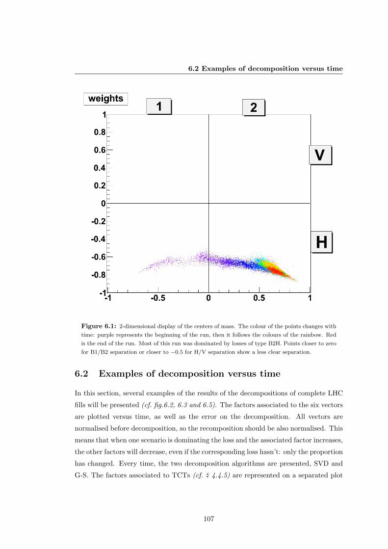
6.2 Examples of decomposition versus time
Figure 6.1: 2-dimensional display of the centers of mass. The colour of the points changes with
time: purple represents the beginning of the run, then it follows the colours of the rainbow. Red
is the end of the run. Most of this run was dominated by losses of type B2H. Points closer to zero
for B1/B2 separation or closer to −0.5 for H/V separation show a less clear separation.
6.2 Examples of decomposition versus time
In this section, several examples of the results of the decompositions of complete LHC
fills will be presented (cf. fig.6.2, 6.3 and 6.5). The factors associated to the six vectors
are plotted versus time, as well as the error on the decomposition. All vectors are
normalised before decomposition, so the recomposition should be also normalised. This
means that when one scenario is dominating the loss and the associated factor increases,
the other factors will decrease, even if the corresponding loss hasn’t: only the proportion
has changed. Every time, the two decomposition algorithms are presented, SVD and
G-S. The factors associated to TCTs (cf. § 4.4.5) are represented on a separated plot
107

6. SPATIAL DECOMPOSITION
(cf. fig. 6.4).
6.2.1 Error propagation for the factors
It was suggested that an error on each decomposition factor could be calculated, in
addition to the error on the decomposition (cf. § 3.5). This is achieved by calculating
the error propagation in the factors for Gram-Schmidt.
Each of the Gram-Schmidt factors fi is defined as the result of the scalar product
between the corresponding reference vector ~vi and the vector of the current loss ~X.
This can be expressed analytically:
fi = ~vi · ~X =
m∑j=1
vij · xj (6.1)
where (xj) are the coordinates of ~X, and (vij) the coordinates of the vector ~vi.
The error on xj , written as σxj , is the error on the measure of the BLM. It is known
to be proportional to the value of the loss:
σxj = 0.01xj (6.2)
The error on the vector ~vi is written as:
σvij =√sys2 + (0.01 vij)2
where sys represents the systematic error on the reference vector. This is known: it
is the standard deviation of each coordinate of the reference vector over all loss maps
composing this vector. It was calculated when the reference vector was created. It
corresponds to the length of the error bar in fig. 4.3, and is the RSD of fig. 4.11,
fig. 4.12 and fig. 4.13 before being divided by the monitor signal. The second term is
the error on the measure of the BLM. Both are independent: one is the error on the
measure from the physical monitor, the other is the error over the different loss maps.
They are consequently summed in square.
Then, the squared error on the factor is calculated as the squared partial derivative
with respect to each independent variable T :
σ2f =
∑T
(∂f
∂T
)2
· σ2T
108

6.2 Examples of decomposition versus time
Figure 6.2: Top: SVD versus time, for transversal and longitudinal loss scenarios and the error
on decomposition, for the stable beam of the 15th of October 2011. Bottom: Gram-Schmidt versus
time. The factors are similar in both cases, and the times at which noticeable changes appear
are exactly the same time. The factors for B1V and B2V in G-S are close to zero, because there
is nothing left of the vector after the projections. As it is often the case, the factor for the L
scenarios are not dominating.
109

6. SPATIAL DECOMPOSITION
Figure 6.3: Decomposition for transversal and longitudinal loss scenarios and the error on
decomposition, for the stable beam of the 22nd of September 2011. Top: SVD versus time,
bottom: Gram-Schmidt versus time. The factors are similar in both cases, and the times at which
noticeable changes appear are exactly the same time. This is an example when the longitudinal
factors actually dominate the decomposition: B1L, dark blue, higher factor at the end of the fill.
B2L is the lower green.
110

6.2 Examples of decomposition versus time
Figure 6.4: Factors calculated for each of the canonical vectors associated to a tertiary collimator
(TCT), for the two decompositions of the stable beam of the 22nd of September 2011. The factor
correspond to the part of the signal at the TCT that wasn’t reconstructed by the reference vectors.
Left: for SVD. Right: for Gram-Schmidt. Bottom: decomposition for Gram-Schmidt represented
in log scale. The factors in both decompositions are equal to a precision of 10−4, and the times at
which noticeable changes appear are exactly the same time. All factors seem to behave similarly
(cf. bottom); the different offsets could be due to the different levels of debris coming from the
experiments measured at each TCT.
111

6. SPATIAL DECOMPOSITION
Figure 6.5: Example of almost constant decomposition for transversal and longitudinal loss
scenarios and the error on decomposition, for the stable beam of the 22nd of October 2011. Top:
SVD versus time, bottom: Gram-Schmidt versus time. This fill was dominated by horizontal
losses for both beams. The factors are similar in both cases, and the times at which noticeable
changes appear are exactly the same time.
112

6.2 Examples of decomposition versus time
which is calculated as:
σ2f =
(∂f
∂vij
)2
σ2vij +
(∂f
∂xj
)2
σ2xj = x2
j · σ2vij + v2
ij · σ2xj
The error on each vector coordinate corresponds to an error on the measurement,
so is also calculated from eq. 6.2.
σ2f =
m∑j=1
x2j ·(sys2 + (0.01 vij)
2)
+ v2ij · (0.01xj)
2 (6.3)
The error on each factor depends on the current loss vector ~X and and has to be
calculated every second. The results are presented in fig. 6.6.
The errors, calculated this way, are too small to affect the final decomposition. They
are dominated by the error on the loss maps, and are at least 3 orders of magnitude
lower than the values of the factors, so they will not be displayed on the results.
Figure 6.6: Error on the decomposition factors calculated by propagation, for the stable beam
of the 22nd of October 2011 (cf. fig. 6.5). The highest error corresponds to the reference vector
which had the highest standard deviation: B2L. All the errors are lower than 3 orders of magnitude
or more of the values of the factors.
113

6. SPATIAL DECOMPOSITION
6.3 Validation of results
In this section, we will show how the results of the decomposition can be correlated
with other validated machine parameters, such as beam measurements of intensity and
emittance.
6.3.1 Beam intensities
All particles measured in the Beam Loss Monitors come from showers initiated by pro-
tons lost from the beam. There is a fundamental link between the decrease of intensity
and the measured losses. However, different events can cause different behaviour: for
instance, a non-noticeable part of the overall intensity lost in a short time at one loca-
tion in the LHC can create losses high enough to trigger a beam dump. In this section,
only beam losses having a noticeable effect on the beam intensity are considered.
Figure 6.7: Intensity versus time, from the 3rd of August 2011 (fill #2000). This plots shows
the readings of the Fast Beam Current Transformers (FBCT) for both beams, smoothed with a
sliding window of 2001 points. During most of this fill, beam 1 lost more particles than beam 2
(the derivative is given in fig. 6.9). The results of the fits are given in eq. 6.13 and eq. 6.14. The
different values in the middle are due to a glitch in the FBCTs.
When considering the decrease of intensity with time over entire LHC runs, i.e. for
114

6.3 Validation of results
periods of time longer than the duration of a loss, one of the first observation is that
the intensity is decreasing linearly with its derivative (with a possible constant):
I(t) ∝ dI
dt(6.4)
Of course, if the intensity derivative is extremely small, the intensity is nearly constant.
This will be shown by measures later (cf. fig. 6.10), but is also rather intuitive: for the
same beam characteristics and optics, if the same proportion of the beam is lost per
unit of time, a beam with a higher intensity will create more losses. This is true at
first order for low values of luminosity, as was the case in 2010. For higher values, at
second order, one should consider the square of the intensity.
The eq. 6.4 can be expressed as a differential equation, with α the proportionality
coefficient:
I(t) ' α · dIdt
I(t) ' I0 · e−αt + C (6.5)
This result corresponds to what is often observed in the beam intensity in the LHC
(cf. fig. 6.7, beam 1, blue). It links to the concept of beam lifetime: the time it would
take for the intensity to reach 1/e of its original intensity. If the constant α is small,
the intensity is seen as linearly decreasing at first order (an example of this behaviour
will be shown later in eq. 6.11):
I(t) = I0 · e−αt + C ∼ I0(1− α · t) + C = −αI0 · t+D (6.6)
In the case of a decreasing exponential, the beam lifetime would correspond to
τ = 1/α. The lifetime calculated for the LHC beams is smoothed to compensate for
the small-scale variations of the beam intensity.
Derivative & smoothing
The first step to investigate the validity of this relation is to calculate the derivative of
the beam intensity. This derivative can be approximated numerically by calculating,
for each value I(t) of the intensity:
δI
δt≡ I(t+ 1)− I(t− 1)
(t+ 1)− (t− 1)=I(t+ 1)− I(t− 1)
2(6.7)
115

6. SPATIAL DECOMPOSITION
Figure 6.8: Left: short period of evolution of the intensity in the LHC as measured by the Fast
Beam Current Transformers, without smoothing, from the 3rd of August 2011. Right: intensity
after applying a smoothing with a sliding window of 2001 points. The small variations were
suppressed, but not the general trend.
The exact derivative would be the limit of this, for δt approaching 0 (and would then
be noted dt). Here, there is only one value per second, so the choice was made to use
only this approximation. For simplicity this value will still be noted dI/dt.
The signal measured by the Beam Current Transformers, representing the intensity
in the ring, is subject to fluctuations: small scale variations of the measured number
of protons, up and down. They should be removed, because they do not correspond
to the actual number of protons: an increase of this number would indicate a creation
of protons in the ring. Moreover, the calculation of a numerical derivative would give
successively positive an negative results: the derivative would not be continuous because
of the discrete measurements. The result would not be fit for visualisation.
These variations can be seen as high frequencies, and can be removed by a low-
pass filter, also called smoothing. The gain from this smoothing is to keep the global
decreasing tendency of the beam intensity, which relates to the loss of protons, while
removing the fluctuations of the instrument.
One way to achieve this smoothing is via a sliding window: each point I(t) is
replaced by the average of all points in the window, noted I(t).
I(t) ≡∑t+n
τ=t−n I(τ)
2n+ 1(6.8)
where n is half the length of the sliding window, which holds 2n+1 points: n points be-
fore, the current point at t, and n points after. The higher the number n, the smoother
the curve. The numerical derivative can then be calculated with less variations. The
results are shown in fig. 6.8.
116

6.3 Validation of results
Figure 6.9: Derivative of the beam intensity of the 3rd of August 2011, smoothed by averaging
in a sliding window with a small number of points compared to the scale of the variations (201
points). The results of the fits are given in eq. 6.10 and eq. 6.11. Note that variations are still
visible, but that both derivatives are clearly negative. The original (non-smoothed) curves were
not fit for visualisation: the pedestals of each side correspond to parts of the curves that were
smoothed with a smaller window.
Another way to avoid small-scale variation when calculating the numerical deriva-
tive is to take a rougher estimation (cf. eq. 6.8) of the derivative:
δI
δt≡ I(t+ n)− I(t− n)
2n(6.9)
where n is half the length of the sliding window. With a high enough number of points,
this restores the continuity of the derivative.
Numerical results
Both techniques lead to very similar results. The evolution of dI/dt versus time is shown
in fig. 6.9. The derivative of the intensity in beam 1 was fitted with the function:
dI1
dt(t) = A · (t− t0) +B (6.10)
A = 3106, 31 p/s2
117

6. SPATIAL DECOMPOSITION
Figure 6.10: Correlation between intensity and its derivative for both beams. The vertical lines
at both ends of the curves are numerical edge effects.
B = −5, 17182 · 108 p/s
EDM = 5.9 · 105 p/s
where t0 is the starting time of observation, and corresponds to 1312346700 s since
EPOCH (origin of database times), and the Estimated Distance to Minimum (EDM)
is the average distance between a point and the fitted function. This is an illustration
of the 1st order approximation presented in eq. 6.6.
The derivative of the intensity in beam 2 was estimated to be a constant:
dI2
dt(t) = −3.44598 · 108 p/s (6.11)
EDM = 47 p/s
The fact that the derivative of the intensity in beam 2 can be fitted as a constant
justifies the use of a linear function to fit beam 2 in fig. 6.7.
To get to the final result, the calculated value of the smoothed derivative at one
time t is correlated with the value of the intensity at the same time t. The results
118

6.3 Validation of results
are shown in fig. 6.10. The derivative of the intensity in beam 1 was fitted with the
function:dI1
dt= α · I(t− t0) + β (6.12)
α = −7.73802 · 10−6 s−1; τ =1
α' 35.9 h
β = 7.20954 · 108 p/s
EDM = 3.1 · 104 p/s
The derivative of the intensity in beam 2 was estimated to be a constant of the
same value as given in eq. 6.11.
Knowing this, the derivative equation 6.12 can be solved as:
I(t) = K · eα·(t−t0) − β
α
which will be simply written as:
I(t) = K · e−t−t0τ + C (6.13)
where C = −α/β. The results of the fit (cf. fig. 6.7) are:
K = 69.3561 · 1012 p
τ = 1, 32969 · 105 s ' 36.9 h
C = 91.8838 · 1012 p
EDM = 2.8 · 1010 p
Note that K +C = 161.24 · 1012 p, which is the value of the intensity at the beginning
of the study (cf. fig. 6.7). The interesting result is that the intensity can be described
as a decreasing exponential, but there is an offset in addition.
The intensity in beam 2 was fitted with the function:
I2(t) = A · (t− t0) + I0 (6.14)
A = −3.42158 · 108 p/s
I0 = 161, 223 · 1014 p
EDM = 1.1 · 108 p
The value of A matches the constant found in eq. 6.11.
In conclusion, the fact that the beam intensity is evolving linearly with its derivative
is a good estimation of the behaviour of the beam.
119

6. SPATIAL DECOMPOSITION
Figure 6.11: Euclidean norm of the loss vector for all BLMs in LHC versus time. The norm
decreases with time.
Figure 6.12: Correlation of the norm of the loss versus the sum of the readings of the BCTs.
Only the “average” value of the norm correlates with the sum of the two beam intensities. The
points for higher values of the norm correspond to occasional higher losses that do not relate to
the intensity, by opposition to “regular” losses which increase linearly with the number of protons.
120

6.3 Validation of results
Dependence of the decomposition on the overall loss
All losses measured by the Beam Loss Monitors come from lost protons: the secondary
particles detected by the BLMs come from primary particles lost from the beam, mostly
on collimators. The norm of the loss vector including all LHC BLMs is shown in
fig. 6.11. If no important loss location is missed, and not too many losses are double-
counted, it should be proportional to dI/dt.
Since the intensity is following linearly to its derivative, the norm of the loss vector
for the whole LHC, reflecting all losses in the ring, should vary linearly with the inten-
sity. This can be seen in fig. 6.12. Since the BLMs can detect the secondary showers
regardless of which beam they come from, the signal of the BCTs were summed up.
The figure illustrates how all previous assumptions on the way to evaluate the total loss
in the LHC and on the behaviour of the beam are justifiable. It can also be assumed
that no important loss location is ignored.
However, this is only true for an average loss and an average intensity: the spikes
seen in the norm (cf. fig. 6.7) correspond to a number of lost protons that is still
small in comparison to the overall number of protons in the beam. The change in
intensity is not necessarily visible. They correspond to “occasional” losses that do not
happen permanently, so they do not relate directly to the value of the intensity (this
corresponds to the cases when big losses are created with little intensity).
6.3.2 Correlation with the result of the decomposition
One simple way to link the results of the decomposition back to direct measurements in
the machine is to consider periods of fills during which the two beams behave differently,
as shown in fig. 6.7: the derivatives of the two beam intensities are different (cf. fig. 6.9).
As explained in § 6.3.1, it means that the losses should be dominated by the beam
losing more protons (Beam 1 in this case). It should show in the decomposition and
the centers of mass.
In order to compare similar values, the center of mass (cf. § 4.5) for the derivatives
is calculated as:
CoM dIdt
=
dB1
dt− dB2
dtdB1
dt+dB2
dt
(6.15)
121

6. SPATIAL DECOMPOSITION
Figure 6.13: Top: Center of Mass calculated for the derivatives of the intensities in both beams
(cf. eq. 6.15), for the stable beams of the 3rd of August 2011 (fill #2000). At the beginning of
the fill, the overall derivative is dominated by the derivative of Beam 1: the center of mass is
positive. The scattered points at the extremities are an edge effect of the smoothing. Bottom:
Center of Mass calculated for the SVD factors (cf. eq. 6.16). This is a two step process, used to
compare similar quantities. At the beginning of the fill, the decomposition is dominated by the
factors associated to beam 1; at the end, the beam 2 factors are more important. The intensity is
smoothed over 2000 points but the losses aren’t, so the small scale variations can’t be correlated.
122

6.3 Validation of results
Figure 6.14: Top: correlation between the Center of Mass calculated for the SVD factors (Y
axis, cf. fig. 6.13 bottom) and the Center of Mass calculated for the derivative of the intensity (X
axis, cf. fig. 6.13 top). When the derivative of the intensity is dominated by beam 1 (CoM closer
to 1), the decomposition is dominated by beam 1 factors (CoM closer to 1). Bottom: correlation
between the derivative of the intensity in beam 1 (Y axis) and the SVD factor associated to B1H
(X axis). For higher values of the factor, many more protons were lost (higher negative values of
derivative).
123

6. SPATIAL DECOMPOSITION
The results are presented in fig. 6.13 top. In this case, the overall derivative is
dominated by the derivative of beam 1 at the beginning of the fill: more protons were
lost by beam 1 than by beam 2. The same process is applied to the results of the
decomposition: a Center of Mass is calculated for the factors of SVD (cf. eq. 6.16).
The results are presented in fig. 6.13 bottom.
CoMSV D =(h1 + v1)− (h2 + v2)
h1 + v1 + h2 + v2(6.16)
Note that this is not the center of mass calculated for the BLM signal at the primary
collimators: this is a two step process, where the SVD decomposition is calculated first,
and then a center of mass is calculated from the SVD factors. This verification was
also done with the center of mass for the BLM signals, and the following results also
apply, but they are not presented here.
The result given by the derivatives of intensities is similar to the result given by
the centers of mass for SVD: the losses are dominated by beam 1. Moreover, the two
curves can be correlated: the more positive the center of mass for the derivatives is
(the more dB1/dt “dominates” dB2/dt), the more dominated by B1 the decomposition
is (cf. fig. 6.14 top). More simply, the factor h1 (dominating the decomposition at the
beginning of the fill) can be directly correlated with the derivative of the intensity in
beam 1, for the entire fill(cf. fig. 6.14 bottom) .
6.3.3 Collimator scraping
One of the beam measurement involving the collimators is the collimator scraping,
described in § 1.4.5. During these measurements, one collimator is moved in the beam,
in order to create high losses. This means that the collimator hierarchy is changed.
In the frame of the decomposition, the corresponding loss profile would then not be
the same as any of the default vectors, since the collimators are in different respective
positions. Conversely, the advantage of this measurement is that the origin of the loss
(particularly the beam plane) is known.
This test was performed during the collimator scrapings which took place in the
night of the 5th of November 2011 (cf. fig. 6.15). The two beams were scraped in
IR7 by their respective horizontal primary collimators. The resulting factors of the
decomposition gives the correct beam and plane and the exact time.
124
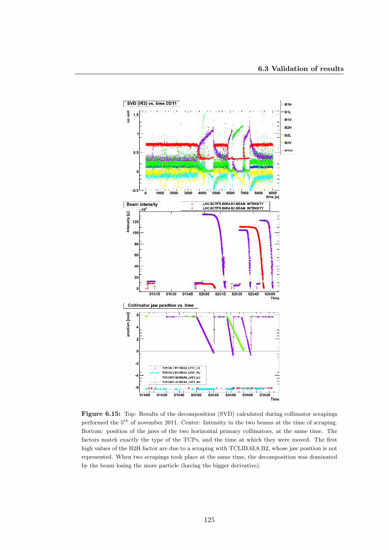
6.3 Validation of results
Figure 6.15: Top: Results of the decomposition (SVD) calculated during collimator scrapings
performed the 5th of november 2011. Center: Intensity in the two beams at the time of scraping.
Bottom: position of the jaws of the two horizontal primary collimators, at the same time. The
factors match exactly the type of the TCPs, and the time at which they were moved. The first
high values of the B2H factor are due to a scraping with TCLIB.6L8.B2, whose jaw position is not
represented. When two scrapings took place at the same time, the decomposition was dominated
by the beam losing the more particle (having the bigger derivative).
125
6. SPATIAL DECOMPOSITION
Further observations show that the observed factor is greater than one. The factor
for the same beam, other plane (depending on the case) is lower than zero: these two
factors compensate each other. This could be explained by the fact that the losses are
higher at the primary collimator than at the other collimators; even higher than in
the standard vector. In order to match this coordinate, the decomposition algorithm
had to give a factor higher than one to this vector. All other collimators have then
a reconstructed signal higher than in the current profile; part of this signal must be
subtracted, leading to a negative factor for the vector associated to the other plane.
Another observation is that the value of the error varies a lot. During “normal”
losses – that is outside the scrapings – the value of the error is rather high: close to
one. This is probably due to the fact that the beam intensity is very slow compared to
nominal operation: only one bunch is injected, for loss security reason. The losses are
then very low (the offset is subtracted), and can not be very well recomposed. However,
during the scraping, the losses increase a lot; and the shape of the vector is then closer
to the default ones, and the loss is better recomposed. This shows that the error is an
efficient way to evaluate the quality of the recomposition.
Another observation is that, starting at 2:35, two collimator scrapings are taking
place at the same time (cf. fig. 6.15 bottom). However, the loss is decomposed in only
one vector at a time: B1H, then B2H, then B1H again. The reason for this is visible
in the plot of the beam intensity versus time (cf. fig. 6.15 center). As explained in
§ 6.3.1, the results of the decomposition correlate with the derivative of the beam
intensity. Fig. 6.15 center shows that there is always one beam losing more protons
than the other at a time. This behaviour corresponds to the results given by the
decomposition.
6.4 Conclusion
Several very different techniques decomposing an unknown loss profile into a sum of
given loss scenarios were presented. All techniques agree with each other. In addition,
the results of these theoretical and non-trivial mathematical operations could be linked
back to the reality of the LHC, such as the beam intensities and their derivatives.
The results were partly confirmed on the scale of the entire LHC, with the tertiary
collimators.
126

Global Conclusion
The goal of this work was to identify patterns in the beam loss profiles, both in their
spatial distribution and in their time evolution.
The first part was achieved by considering the profiles as vector, using both vector
projection (Gram-Schmidt) and matrix inversion techniques (Singular Value Decompo-
sition). Different studies proved that it was possible to identify patterns in a measured
loss profile, considering limitations such as the quality of the recomposition and the
choice of the patterns. The extracted information must always be considered with these
limitations: a good decomposition on wrong vectors, as well as a bad decomposition
on good vectors could lead to wrong conclusions. The selection of the reference vectors
proved to be a key aspect. patterns corresponding to specific loss mechanisms were
identified: the scenarios corresponding to the 3 planes of the particle coordinates for
the 2 beams.
The second part, the time evolution, helped understanding how to consider the dif-
ference between vectors. Averaging the monitor signals over a long period of time lead
to the creation of a default loss profile. It showed that most Beam Loss Monitors have
a rather constant behaviour; the decomposition focuses on the monitors which don’t.
Most of the non-nominal losses which are not covered by the spatial decomposition
could still be noticed by comparison with the default loss profile. A way to evaluate
the error on the recomposition was developed, in order to investigate the correctness
of a decomposition. It lead to the implementation of a “threshold” between good and
bad decompositions. The results were cross-checked with other beam instruments and
measurements.
The decomposition techniques have been implemented by other people in a real-
time instrument, which can be used to help machine operation, by helping to identify
the origin of a loss at a given time and detecting unusual losses. Further work would
127

6. SPATIAL DECOMPOSITION
include adding more default vectors for different situations. For instance, reference
vectors could be created for all possible beam modes in addition to stable beams, and
for the ion fills. The decomposition could be performed on all past and future “stable
beams” periods, to learn about the global evolution of the behaviour of the LHC.
New reference vectors could be produced for other scenarios, such as a breaking of the
collimators hierarchy. Implementing the comparison with the default loss profile in real
time would help evaluating how “standard” the current loss is.
Different vectors could be produce also by changing the selection of monitors, or
using different integration windows. Other decomposition algorithms could be added,
such as the Gram matrix, blind signal separation or data fits that would return only
positive factors.
Eventually, this tool could be used in other machines having loss monitors and in
which loss profiles can be measured. This doctoral work, with its limitations, could help
the operation of particle accelerators by extracting information on the beam dynamics
from the global beam losses.
128

Appendix A
Data Access
A.1 Introduction
A.1.1 Beam losses
The Beam Loss section at CERN has installed more than 3600 Beam Loss Monitors
(BLMs) around the LHC ring, in order to measure the beam losses in the LHC. If the
losses exceed the set loss thresholds, the beam permit is removed, and the beam is
removed from the ring and directed towards a beam absorber. The whole process is
called a dump, and must be triggered in less than one turn of the LHC: 89µs.
The BLMs are installed in expected loss locations, given by simulation and a good
understanding of the beam optics in the LHC. Finding the origin and the reason of a
beam loss (whether it lead to a beam dump or not) is crucial to the further under-
standing of the beam optics, as well as the good functioning of the LHC.
All data produced by the BLMs are used in real time, for threshold comparison;
then some is stored in the LHC databases, which will first be further described below.
However, the layout of the machine where the loss was produced is just as important
as the measured loss itself, and must be understood as well.
A.1.2 Introduction to the Beam Loss Analysis Toolbox
The Beam Loss Analysis toolbox was designed to allow the access, processing and display
of data in a fast, user-friendly and easy way. This chapter describes the techniques used
to access the different databases, to combine the values of losses with the position of
the BLMs and magnets, and their display. The ensemble of these techniques is referred
129

A. DATA ACCESS
to as a toolbox. The toolbox was then expanded to process and display other beam
instruments than the BLMs.
The main programing and data analysis framework at CERN is ROOT, a C++
framework providing classes and a C++ interpreter called CINT. Amongst other,
ROOT provides objects that can send SQL statements and receive the results.
The choice was made to use Python (2.4) as the developing language (and not
CINT), since a true interpreter was desirable. It links easily with ROOT (5.28) objects
thanks to the pyROOT project.
The toolbox was developed in a way as object–oriented as possible. It is made
of several modules, holding different classes and functions. The classes hold methods
that are functions bound to the object, and attributes that are variables stored in
the object. Additionally, specific structures were created and are common to several
objects, simplifying the communication between objects and the understanding of the
user.
The main modules are:
� databases;
� analysis;
� display.
The databases module provides all the classes to connect to the different databases,
and get the data in specific formats. The language used for database access at the
time of development was PL/SQL, so the access was first done using Structured Query
Language (SQL) queries. Then, a new Application Programing Interface (API), written
in Java, was implemented for the Logging and Measurement databases by the databases
management in order to protect them. It avoids having a direct access of the databases
by the user (dangerous for the databases) by implementing a “tier 3” access via a server
running the API. The access to the Layout database is still achieved via SQL queries.
The display module provides classes taking data in the format returned by the
databases module, and plots them on screen. It allows a simple management of several
graphs in one scope.
The analysis module is “wrapping” class that uses classes and methods provided
by all the other modules so that the user can display losses in a section the LHC at
130

A.2 Data & databases
one timestamp, in only one command line. It also accesses other modules dedicated to
other instruments in the LHC.
A.2 Types of required data and
corresponding databases
Before describing the structure of the modules, the different type of data (signal or lay-
out data) must be presented, as well as the storage structure of the different databases
holding these data.
A.2.1 Data structure
Running sums
The Beam Loss Monitors are ionisation chambers. The BLM electronics reads the
output of the chamber every 40 µs, permanently. These values are then summed up
following different integration intervals called running sums (cf. tab. 2.1). The resulting
values corresponds to the charge deposited in the chamber after applying conversion
factors.
Every second, for each monitor, one value per running sum is selected to be stored
in the Measurement database. For the running sums shorter than one second (1 to
8), the selected value is the highest in the last second; for the others (9 to 12),
the last value is selected. The running sums are stored under a specific variable
name: BLM_EXPERT_NAME:LOSS_RSXX, where "BLM_EXPERT_NAME" is the official name
of the BLM following the naming convention, and "RSXX" is the running sum name
(cf. tab. 2.1).
Two SQL lists are associated to each variable: the list of timestamps (date and time
at which the data was taken) and the value at that timestamp (cf. §. A.2.3).
Thresholds
The loss thresholds are different from BLM to BLM, depending on the element they
protect; they also change depending on 32 levels energy of the beam and the LHC cycle
phases.
131

A. DATA ACCESS
The current thresholds used at one time are stored in the databases, under a
variable name similar to the one of the loss: BLM_EXPERT_NAME:THRESH_RSXX where
"BLM_EXPERT_NAME" is the official name of the BLM, following the naming convention,
and "RSXX" is the running sum name (cf. tab. 2.1).
A.2.2 Layout database
The Layout database holds most of the layout information about the LHC. In this case,
the relevant information includes:
� position of the BLMs;
� position of the beginning and the end of magnets;
� position of the collimators;
� position of other beam instruments;
� optics variables.
This information is essential to the good understanding of the losses, in order to
show where it happened, and what element of the LHC can have created it.
The structure of the Layout database is the one of a standard SQL database: sev-
eral tables hold all related information in different columns. For instance, the col-
limator positions, in column TC_POSITION, are linked with the collimator names in
the column TC_OFFICIAL_NAME, and they are both stored in the table which is called
COLLIMATOR_STRUCTURES.
A.2.3 Measurement database and Logging database
Data storage
Two identically behaving databases are used to store the values coming from the beam
instruments of the LHC. The first one, called Measurement database (MDB), gives a
temporary storage (one week) to all selected data (cf. § A.3.1). Then, an algorithm
specific to each system selects which data will be send to the Logging database (LDB)
to be stored permanently.
For the “loss” values, the data are stored permanently in the Logging database after
applying a filter: if the difference between two subsequent values is higher than a delta
132

A.3 Database Access Techniques
set per Running Sum, the value is saved; if not, one value per minute is saved. This
makes sense because during regular running of the LHC, when the losses are minimal
and don’t fluctuate much around the basic offset, only a few data are logged. When
losses do appear, the values are higher than the basic offset, and it is important to log
all of them.
However, one must understand that data from each BLM are not all logged at the
same timestamp. This is described in fig. A.3 and an example is shown in fig. A.5 where
one point corresponds to one logged value: they are not logged at the same second in
a minute.
For the “threshold” values, the data are logged “on change”: a value is logged only
if it differs from the previous one, and once per day if they don’t change.
Data types & views
Because of their sizes, of the fact that they are written and read permanently, and
contrary to layout data, the measurement data do not follow the basic table / column
/ element structure. They are stored following their data type in different tables called
views. The views are different ways of getting the same data, e.g. all data in the time
range, or only last data in the time range. All possible views are described in (16).
Each table only has few columns, including UTC_STAMP, giving the timestamps at
which the data was logged, and VALUE. The name of the variable itself is not stored
there. The variable name and the time range, the query parameters, have to be set
before requiring the data from the relevant view (17).
A.3 Database Access Techniques
In this section, the module used to access databases is described, as well as the tech-
niques implemented in the tool.
A.3.1 PL/SQL Access
The first way to access the Measurement and Logging databases was via an API written
in PL/SQL, providing a direct access to the databases (17).
133
A. DATA ACCESS
Connection — passwords and security
In order to access each database with SQL statements, user names and passwords
specific to each database must be provided. In addition, the access to Logging and
Measurement databases requires a client identification and an application name.
For obvious security reasons, these are not hard-coded in the modules. They are
stored in a specific separated file which is not distributed and is specific to each user.
The default python module ConfigParser (18) provides the retrieving of the values
in the file. It is embedded in a method belonging to the superclass of all databases
classes. The details are stored as attributes of the class and used to open connections.
The classes dealing with Logging and Measurement databases leave the opening and
closing of connection to the user; all other classes do it automatically.
The connection is opened via an object imported from ROOT and called TSQLServer
(19). The user and password are passed to the Connect method, which returns a pointer
to the TSQLServer object. It is stored as an attribute called sqlData and will be used
to send queries (cf. § A.3.1).
For Measurement and Logging databases, the client identification and the applica-
tion name had to be passed in addition. The SQL query was the following:
DECLARE
l_client_id varchar2(30) := ’YOUR_CLIENT_ID_HERE’;
l_app_name varchar2(30) := ’YOUR_APP_NAME_HERE’;
BEGIN data_access.set_client(l_client_id, l_app_name); END;
The reason for these classes to be able to open and close connection themselves is
that the Logging and Measurement databases are protected in access. One could not
open more than 500 “tokens”, one token corresponding to the query of one variable.
If the user requested more than 500 variables, the connection object would close the
connection after 500 variables, and then open a new connection.
Note that after moving to the java command line application to access the Log-
ging and Measurement databases, these operations were not needed any more. The
application deals with the opening and closing of connections.
134

A.3 Database Access Techniques
PL/SQL Queries
Once the connection is opened, queries can be sent. This is achieved the attribute
called sqlData. It is used to communicate with the database by sending SQL queries
that are automatically constructed as strings, e.g.:
select TC_OFFICIAL_NAME, TC_POSITION from COLLIMATOR_STRUCTURES;
Sending a query with a TSQLServer object returns a TSQLStatement object. It can
be iterated by the NextResultRow() method, and the contents of each row (two in the
previous example) are returned by the GetString(i) method (19).
The values are always returned in order as strings so the user does not have to
change the ROOT method depending on the data. Instead, a function of databases
will automatically cast it as an integer if possible, or a float if not possible, or leave it
as a string if both castings fail.
Query Parameters
For the Measurement and Logging databases, the query parameters have to be set before
starting the data query; that is, the time window and the variable names (cf. § A.1.2).
The time window is set by a single method, that sends the following query:
begin data_access.SET_TIME_WINDOW(:1, :2); end;
where “:1” and “:2” are the positions of the arguments, coded by an integer in the
call of the TSQLStatement.SetString(i, str) method. Note that the numbering of
the arguments starts at 1 in the SQL query, but starts at 0 in the ROOT function.
The variable names are passed the same way, starting with the query:
begin data_access.SET_VARIABLE(:1); end;
and followed by the actual variable name is passed with the same TSQLStatement
method. Then the actual timestamp and values are requested by the query:
select utc_stamp, value from var_numeric_data_v
where var_numeric_data_v can be any “view” described in (16). Again, the results
are returned by the TSQLStatement.SetString(i, str) method iterating over all
timestamps in the time window.
135

A. DATA ACCESS
Variable lists
The database access services provide a way to save variable lists, in order to make the
querying of repeated series of the same variables easier and faster. Variable lists have
to be created beforehand and saved under a user name. However, once created, they
are fixed: they won’t follow the evolution of the variables in the database.
The querying of variable lists is similar to the querying of separated variables, the
differences being: the views (16), and the fact that each variable name has to be queried
as well:
select variable_name from variable_list_variables_v
All lists had to be created by direct SQL access to the databases using sqlplus, and
where filled using another module which is not described here.
A.3.2 Java access
The current way to access the Logging and Measurement databases is through the pro-
vided Java API. It provides an additional layer between the user and the databases,
protecting them and dealing with all the security requirements. The Java API is origi-
nally designed to write applications in Java. In addition, it allows being called from the
command line, thus being more portable: the data are not returned inside one specific
application, they are written to the shell standard output.
The use of this command line is further described in (20).
Connection and security
The Java API provides all the opening and closing of connections, so the user does not
have to deal with it. It also provides the user names and passwords for the Logging
and Measurement databases.
Most of the connection configuration settings, including the client ID and applica-
tion name, are written in a file called configuration.properties (20). A different
name can be passed in the command line, allowing different pre-saved configurations.
However, rather than having the user edit this file separately, this file is generated
automatically. It allows a more advanced behaviour, and backward compatibility. For
instance, if the user requires data from the Measurement database, but with a date
136
A.3 Database Access Techniques
older than a week, the tool switches to Logging database automatically, instead of
returning empty objects.
Data request methods —
Calling a command line from python
The command line API currently provides two methods to access data: DS (DataSet,
all data in time range) and LD (Last Data during or before the given time range). The
“data or last” view in SQL, that was returning all data in range if any, or the last data
before range if not, is not implemented.
The time range is passed as two options, -t1 and -t2, and the dates must have the
format "YYYY-MM-DD HH24:MI:SS". Dealing with the dates is done with the Datime.py
module, which was written on purpose.
The standard way to access the data is via the -O option. The data are then
written in the standard output of the shell. The default python os module provides
the interaction with the shell from python. The os.popen function takes the command
line as a string, which allows easy string manipulation. It returns a file iterator, which
is the same type as the object return by the default function open opening files. The
data flow is described in fig. A.1.
This object can then be iterated over line by line, since they are strings. The main
limitation is the rather small memory limit (with respect to the amount of data consid-
ered here) of the Java heap: 250 Mb, which corresponds to only 15 mins of measurement
data for the whole ring.
Passing variables is done with the -VS option followed by all variables separated by
commas. There is apparently no limitation on the number of variables: all BLMs in
the LHC can be queried at once. The only limitation is the total size of the data set.
The Java command line API provides an extra functionality: it allows to write the
data directly in a file. The filename is passed with the -N option, and the type with
the -F option.
The command line has the ability to cut a dataset into subsets, in order to allow the
downloading of amounts of data bigger than the memory limit. This is done using the
-IT (Interval Type) option, together with the -NI (Number of Intervals) option. For
instance, passing “-NI 15 -IT MINUTE” will cut the dataset in slices of 15 minutes.
137
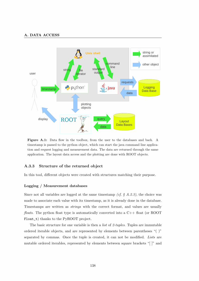
A. DATA ACCESS
LoggingData Base
requests
data
Unix shell
display
user
standard output
command line
fileiterator
string
plotting objects
timestamp
string or assimilated
other object
LayoutData Bases
query
data
Figure A.1: Data flow in the toolbox, from the user to the databases and back. A
timestamp is passed to the python object, which can start the java command line applica-
tion and request logging and measurement data. The data are returned through the same
application. The layout data access and the plotting are done with ROOT objects.
A.3.3 Structure of the returned object
In this tool, different objects were created with structures matching their purpose.
Logging / Measurement databases
Since not all variables are logged at the same timestamp (cf. § A.2.3), the choice was
made to associate each value with its timestamp, as it is already done in the database.
Timestamps are written as strings with the correct format, and values are usually
floats. The python float type is automatically converted into a C++ float (or ROOT
Float_t) thanks to the PyROOT project.
The basic structure for one variable is then a list of 2-tuples. Tuples are immutable
ordered iterable objects, and are represented by elements between parentheses “( )”
separated by commas. Once the tuple is created, it can not be modified. Lists are
mutable ordered iterables, represented by elements between square brackets “[ ]” and
138
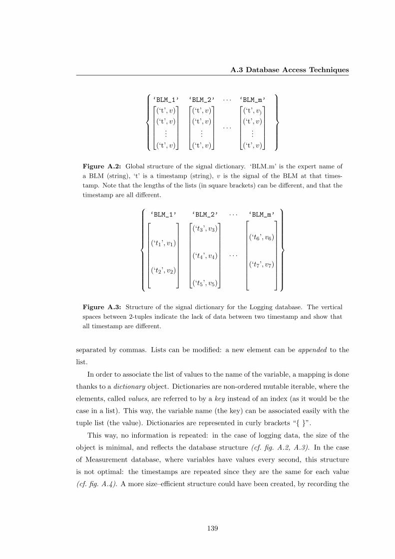
A.3 Database Access Techniques
‘BLM_1’ ‘BLM_2’ · · · ‘BLM_m’(‘t’, v)
(‘t’, v)...
(‘t’, v)
(‘t’, v)
(‘t’, v)...
(‘t’, v)
· · ·
(‘t’, v)
(‘t’, v)...
(‘t’, v)
Figure A.2: Global structure of the signal dictionary. ‘BLM m’ is the expert name of
a BLM (string), ‘t’ is a timestamp (string), v is the signal of the BLM at that times-
tamp. Note that the lengths of the lists (in square brackets) can be different, and that the
timestamp are all different.
‘BLM_1’ ‘BLM_2’ · · · ‘BLM_m’(‘t1’, v1)
(‘t2’, v2)
(‘t3’, v3)
(‘t4’, v4)
(‘t5’, v5)
· · ·
(‘t6’, v6)
(‘t7’, v7)
Figure A.3: Structure of the signal dictionary for the Logging database. The vertical
spaces between 2-tuples indicate the lack of data between two timestamp and show that
all timestamp are different.
separated by commas. Lists can be modified: a new element can be appended to the
list.
In order to associate the list of values to the name of the variable, a mapping is done
thanks to a dictionary object. Dictionaries are non-ordered mutable iterable, where the
elements, called values, are referred to by a key instead of an index (as it would be the
case in a list). This way, the variable name (the key) can be associated easily with the
tuple list (the value). Dictionaries are represented in curly brackets “{ }”.
This way, no information is repeated: in the case of logging data, the size of the
object is minimal, and reflects the database structure (cf. fig. A.2, A.3). In the case
of Measurement database, where variables have values every second, this structure
is not optimal: the timestamps are repeated since they are the same for each value
(cf. fig. A.4). A more size–efficient structure could have been created, by recording the
139

A. DATA ACCESS
‘BLM_1’ ‘BLM_2’ · · · ‘BLM_m’(‘t1’, v)
(‘t2’, v)...
(‘tn’, v)
(‘t1’, v)
(‘t2’, v)...
(‘tn’, v)
· · ·
(‘t1’, v)
(‘t2’, v)...
(‘tn’, v)
Figure A.4: Structure of the signal dictionary for the Measurement database. Note that
all timestamps in each “line” are the same; all values are different.
timestamps separately, but it would have implied a different processing of measurement
and logging data. The choice was made to keep the same structure for both databases.
This object is referred to as signal dictionary (cf. fig. A.2, fig. A.3).
The non-ordering of dictionaries is part of the characteristics of the object, and
done on purpose by a randomization of the keys to insure that one is never in the worst
case (in an algorithmic efficiency point of view) when accessing elements. However, the
list of keys can be ordered.
Layout databases
In the case of layout databases, several columns can be queried at once. In this case,
the get_from_layout method returns a dictionary with one key per column, associated
to a list of the values returned by the database (cf. § A.3.1). The fact that all lists
have the same length is insured by the structure of the database. The structure of the
object reflects the structure of the database.
This structure is general but not the most adapted to all situation. New and
more adapted objects are created later. For instance, in the case of magnets, three
variables are required: the magnet name, the magnet start and the magnet end. The
reconstructed object is a dictionary where the key is the magnet expert name and the
value is the 2-tuple (start, end).
A.4 Display
In this section, the different objects in the display module are described. This objects
are made to take the objects returned by other functions and classes in other modules.
140

A.4 Display
A.4.1 Plotting with ROOT
When the modules were developed, the best option to produce plots and graphs was
to use ROOT objects. ROOT provides graphical objects that are straightforward to
use in a global scope, i.e. in a ROOT script interpreted by CINT or in the python
interpreter; however, using them in functions and classes requires more care.
The main object for scatter plots is called TGraph (21). The latest versions of
ROOT do not require to know the number of points beforehand any more; the points
can be set on the fly. The object corresponding to the window on the screen is called
TCanvas. Both the TGraph and TCanvas object must exist in the current scope for the
graph to be seen.
The TGraph::Draw() method will automatically create a TCanvas if no one has
been created before. However, this specific TCanvas is not returned: if this method is
called in any other scope than the global one, the TCanvas will consequently be deleted
when exiting the current scope. Moreover, if another TCanvas was created before, and
held a different graph, its graph will be replaced.
If the TCanvas is returned, but not the TGraph, the graph will be deleted when
exiting the scope, thus disappearing from the TCanvas, leaving and empty window.
The correct way to proceed is to first create a TCanvas, then draw the TGraph on
it, and return or save both. This way, they stay visible for the user as long as the code
is running. The choice was made to store them as attributes of the different plotting
classes. This way, the user can have several instances of the class achieving the same
type of display.
A.4.2 Signal vs. time
Reflecting the data structure — multigraphs
The first plot (and most related to the database structure) is the display of all data
versus time. It is created from the signal dictionary (cf. § A.3.3). One TGraph object
is associated to each variable.
For each 2-tuple of the list associated to each variable, a Datime.datime object is
created, corresponding to the current timestamp. This object has a Convert() method
that returns the number of seconds since epoch at that time. This is used as the X
coordinate, the Y coordinate being the second element of the 2-tuple. The axes of the
141

A. DATA ACCESS
TGraph have a TAxis::SetTimeDisplay() method that will convert this number back
into human-readable time and date.
Figure A.5: Example of “plot time” object: signal of BLMs versus time. One graph and
one colour is associated to each BLM. The X axis displays date and time in human-readable
format. The BLMs are ordered in the legend, and in colours. One specific timestamp can
be indicated on the plot by a vertical line; the requested timestamp is displayed by default.
All the TGraphs are stored in an attribute of the object: a dictionary called graph-
dict, where the key are the variables, and the values are the TGraphs. All TGraphs
are gathered in a TMultiGraph object. Each TGraph gets a specific colour as different
from the others as possible. All this and the creation of the TLegend is done by the
display.rainbowplot function.
Rainbow plots
In ROOT, colours are coded as integers. The first integers (0-9) give a range of basic
colours, but higher values (51-100, 200-228) give a smoother colour range. In order that
all graphs have colours as different to each other as possible, the colour range is divided
into n − 1 ranges of equal lengths, where n is the number of graphs. For instance, if
there are 3 graphs, the first graph gets the first colour of the range, the second gets
142

A.4 Display
the colour of the middle of the range, and the third gets the last colour. Graphs can
be ordered for clarity: in this case, an ordered list of names has to be passed.
The legend is created at the same time, its length depending on the number of
graphs. If there is only one graph, the colour is black.
A.4.3 Plotting the LHC
One of the current main application of the toolbox is a longitudinal loss profile of a
section of the LHC at a requested timestamp. This needs the position of the magnets
and collimators, obtained from the Layout database. The signal of the BLMs is mapped
to their longitudinal position in the LHC, called DCUM, which are obtained from the
same database. The results are shown in fig. A.7.
Format of the “plot LHC” data
The format of the data taken by this plot is the following: the basic 2-tuple (couple)
of values is: (DCUM, value of the loss at the displayed timestamp). The names of the
BLMs are not displayed, but they contain all relevant information: type of monitor
(Ionisation Chamber (IC) or Secondary Emission Monitor (SEM)), associated beam
(B1 or B2), injection or extraction line. The sorting of the monitors according to these
criteria will be described in § A.5.2.
The structure of the data object, called plotdict (cf. fig. A.6), reflects this sorting:
to each graph name is associated a list of 2-tuples: (DCUM of the monitor, signal of
the monitor at the plotting time). The creation of this object is done in the process
module (cf. § A.5.2).‘name_of_graph_1’, ‘name_of_graph_2’, · · ·
(dcum1, v1)
(dcum2, v2)...
,
(dcum3, v3)
(dcum4, v4)...
, · · ·
Figure A.6: Global structure of “plotdict” object. dcum1 is the position of BLM1, and
v1 the signal of BLM1 at the plotting time.
Because of the very wide dynamic range of the BLMs (106), the signal (Y axis) is
nearly always displayed in logarithmic scale. However, for some reason, this is a method
143

A. DATA ACCESS
of the TCanvas object and not of the TAxis, regardless if the canvas holds a graph or
not. The canvas being stored as an attribute, this method can still be accessed.
The plotting time is an important value that is displayed in the title of the plot.
The thresholds can be displayed on the same plot. They have the same structure,
and will be plotted on the same scale, with the same X coordinate (DCUM) of the
BLM they correspond to, in a different colour (green).
The colours of these graphs follow the plotting convention of the LHC: graphs
related to beam 1 are plotted in shades of blue, and those related to beam 2 in shades
of red. The plot_LHC._set_graphs_with_conventional_colours method holds all
the mapping of the different graph names to the correct colour.
Figure A.7: Example of “plot LHC” object: longitudinal loss at one timestamp (given in
the title). The X coordinate gives the longitudinal position of one BLM; the Y coordinate
gives the value of the signal or threshold of this BLM. The plot is only made of four graphs:
two for the BLM signals and two for the thresholds. The magnets are displayed as blue
boxes, the collimators as red ones. The plotting time and the running sum are displayed
in the title.
In addition, the object must have the position of all collimators in DCUM range, and
the positions and lengths of all magnets in range. They can be passed in the constructor;
if not, the object has the possibility to create a databases.ConnectionToLayout object
144
A.4 Display
(cf. § A.3.1) that will get the details of all collimators and magnets in the DCUM range.
Display of the magnets and collimators
Magnets and collimators are displayed on the graph using the ROOT TBox objects.
The constructor takes the coordinates of top left an bottom right corners, and these
coordinates can be expressed in the same range as the coordinates of the graphs: the
TBoxes will then follow the zooming in and out in the plot. Magnets are plotted with
their real lengths, since it provided in the database, whereas collimators just have one
position recorded in database. They are all plotted with an arbitrary length of 1 m,
which is close to reality. Magnets are displayed in blue, and collimator as smaller red
boxes.
The Y coordinate of magnets and collimators can be specified so they are conve-
niently displayed whatever the scale of the plot is. By default for LHC losses, the boxes
are arbitrarily displayed between 10 and 50 Gy/s.
Display of the cell names
Another information to display would be the cell name. It tells which half-octant of
the LHC is considered, and the number of the cell in this half octant. A cell is the basic
pattern which is repeated in the arcs to create the whole ring: that is, three dipoles
and a quadrupole. The ROOT object to display text, the TPaveText, can be created
the same way as a TBox, following the plot coordinates; however, once created, it will
not follow the zooming in and out of the plot. It can only be seen when a small portion
of the LHC is requested: the cell names are only displayed if the displayed section
corresponds to less than 30 cells.
A.4.4 XY plots
The display modules provides a class creating a scatter plot, with the same conven-
tions, attributes and method as the other plots. The data as passed in a plotdict
dictionary, where the key is the name of the plots and the value is a list of 2-tuples,
each 2-tuple being the coordinate of one point.
145

A. DATA ACCESS
‘name_of_plot_1’, ‘name_of_plot_2’, · · ·RS01
RS02...
RS12
RS01
RS02...
RS12
· · ·
Figure A.8: Global structure of the running sums dictionary. RS01, . . . , RS12 are the
values of the twelve running sums; usually, a plot will display all running sums for one
monitor, or the thresholds of a family of monitors.
A.4.5 Plotting Running Sums
The display in one graph of all the running sums of the same monitor versus the corre-
sponding integration duration is a recurrent requirement. A class has been specifically
designed to fulfill this requirement.
Format of the RS data
The duration of each running sum is a fundamental value of the BLM system (cf. § A.2.1).
These values are hard-coded in a list, which is a global variable for the module and can
be accessed all the time. The number of the running sum is coded by its position in
the list. For human-readability purposes, the indexing of the running sums starts at 1,
matching their names (the first element of the list is zero).
The structure of the data object is a dictionary, where the key is the name of the
graph, and the value is the list of values for each running sum, coded by position.
Conventions for plotting
The conventions for plotting running sums are the following: the duration is represented
on the X axis in logarithmic scale; the dose per second is represented on the Y axis in
logarithmic scale. The 12 dots are linked by a line.
This way, a flat line represents a constant dose per second deposited in the ionisation
chambers, while the loss is occurring; a line of slope −1 shows that all the dose was
deposited, and that the same deposited dose is being integrated over longer and longer
integration windows.
146

A.5 The wrapping module: analysis
A.4.6 Methods shared by all plots
All plots inherit from the same class, called superclass_plot. This class has several
methods.
Title & plotting time
The smallest piece of information to describe a loss is its timestamp: it is unique
for each loss. It is thus displayed in the title. The Datime.datime object provides
different formats to print a timestamp, one of them being called the “short” format:
YYYYMMDD-HHMMSS (returned by the datime.print_short method). This format is used
in the title. If no title is specified, one is automatically created, being the short format
of the plotting time. The user has the possibility to add more details about the loss:
the type of loss, the section of the LHC that is displayed, or anything passed as a string
in the argument called additional.
Saving
All plots come with a save method, in order to make the saving of plots easy for the
user. This method will automatically generate a meaningful file name, matching the
title of the plot, and save it in the ~\public folder.
In the simplest of cases, the method myplot.save() can just be called and the
plot will be saved just as it is seen on screen, with a unique and relevant name. An
additional string and a saving path can be specified.
A.5 The wrapping module: analysis
In order to avoid having to create many different objects, call many different methods
and use different attributes, and wrapping class has been created called analyse, in the
analysis module. It creates automatically all the different connection objects, gets
the relevant data in the correct format, passes the data objects to the plot objects, and
holds the resulting plots as attributes. All these attributes are described in tab. A.1.
147

A. DATA ACCESS
A.5.1 Basic behaviour
Introduction: list of arguments
The basic behaviour of the analyse class is to display the longitudinal development of
one loss appearing at one timestamp in a section of the LHC, getting the data from the
Logging database (cf. § A.2.3). The constructor needs to take at least one argument:
the time of the loss, called plotting time. The time range for data download is centered
around that time.
A specific section of the LHC can be specified by passing two values of DCUM. Only
the data concerning the BLMs, magnets and collimators within this DCUM range will
be downloaded. The number of the running sum can be specified, as well as flags
(boolean values that are only true or false) controlling the inclusion of thresholds or
SEMs.
All the actions described in this section are performed automatically.
Creation of the list of BLMs
When plotting only a section of the LHC, there is no point requiring all monitors in
the ring, as it is a time-consuming operation. Only the monitors within the specified
DCUM range are required. The choice was made that the user only passes the DCUM
range as an extra argument; if no range is passed, the default value of the arguments
selects all BLMs.
At the beginning of the run of the LHC, the list of BLMs details in the databases
was updated regularly. The choice was made to not have the list of BLMs written in a
file, but to generate it from the database once per day. This list (ordered by DCUM)
is downloaded from one of the layout databases called MTF. If no list was created that
day, the tool creates the list and saves it in a temporary file holding the date. If the
file already exists and has the correct date, the tool reads the data from the file. The
list is not generated every time for speed reasons.
Once the list is generated, the names of the BLMs in the DCUM range are selected
and stored as an attribute.
148

A.5 The wrapping module: analysis
Data query
Once the list of BLMs is created, a connection object is created (cf. § A.1.2). The
default is a connection to the Logging database, but the user can ask to connect to
the Measurement database. The data are queried with the current time window, the
current list of BLM, and the given running sum value. The returned object is called
“signal” dictionary. The structure of the signal dictionary is described in fig. A.2. The
next step is to extract the signal of the chambers at the required time.
Getting the exact second — Case of the Logging database
Once the data are downloaded, the losses as the specified time must be extracted.
This extraction is achieved by the process module. The corresponding algorithms are
described in § A.5.2.
Preparation of the data for plotting versus DCUM
Plotting all BLM signals together versus BLM position would not display relevant
information. The BLMs have to be separated depending on their type: if they are
ionisation chambers or second emission monitors, if they belong to beam 1 or beam
2, or if they belong to the dump line or not. The corresponding thresholds are sorted
accordingly. The sorting is done in the process module. The structure of the “plotdict”
object is described in fig. A.6.
Plotting
Once all the data are gathered and put in the proper formats, they are displayed on
screen.
The analyse.Signal object (cf. fig. A.2) is passed to a display.plot_time object
(cf. § A.4.2), and the result is stored in the attribute analyse.TimePlot.
The plotdict object (cf. fig. A.6) is passed to an object of type display.plot_LHC
(cf. § A.4.3) and stored in the attribute analyse.LHCPlot.
The plotting can be disabled for speed purposes by passing a the default argument
PlotOut as False.
149
A. DATA ACCESS
A.5.2 Process
Most of the data processing required in order to display a loss in a section of the LHC is
done in the process module: finding the value of the loss at the plotting time, creating
the “plotdict” object holding the data (cf. fig. A.6) and sorting the BLMs by type.
Weighted averages
As explained in § A.2.3, BLMs don’t have data logged every second in the Logging
database. If a big loss (bigger than the set delta) occurred at the time of plotting, data
will be recorded for this specific second; but if no loss appeared on some BLMs, only
one data per minute is recorded. In case of no loss, the choice was made to use a linear
interpolation between the previous and the next recorded values. This makes sense
because the fact that no data was recorded is a proof that the signal did not change
more than the delta. The difference between the real signal and the recalculated signal
is within the fluctuations of the signal, thanks to the tuning of this delta.
The choice of the algorithm finding data at a timestamp in a list of tuples or cal-
culating the linear interpolation is very crucial, as it is heavily used in certain analyses
looping many times over the same dataset.
Linear interpolation. The first algorithm was one that can be used both on mea-
surement and logging data. It takes the reference timestamp, a list of tuples, and
progresses through the list. If the same timestamp is found, the value (second element
of the tuple) is returned. If not, the next (and newer) timestamp is taken, and the
linear interpolated is calculated, following:
vreq =v2 − v1
t2 − t1· treq +
t2 · v1 − t1 · v2
t2 − t1
where treq is the reference time; vreq is the value at treq; (t1, v1) are the timestamp and
value of the point (tuple) before tref ; (t2, v2) are the timestamp and value of the point
(tuple) after treq.
The result returned is the maximum between the signal and a non-zero value (usu-
ally set at 10−9, lower than the lower possible signal) in order to avoid zero values, which
can not be displayed in logarithmic scale. All results are gathered in a One Value Dic-
tionary (OVD), where keys are BLM names and values is the calculated signal at the
plotting time.
150
A.5 The wrapping module: analysis
Speed. The speed of this algorithm is roughly O(m · n), where m is the number of
monitors (the algorithm has to loop over monitors) and n is the index of the second
(the algorithm has to go through all tuples from the beginning till the tuple holding the
proper timestamp). For speed reasons, the algorithm does not go through all seconds
every time: when the next timestamp has been found, the looping stops.
The processing time is dominated by the data access time in the case of the Logging
database, when only one second is requested in a time range composed of a few tuples.
Very big time windows are rarely requested. However, during statistical analysis, when
all seconds are considered, the running time diverges when reaching the last seconds of
the dataset.
Different consideration of Measurement database. Searching for a specific sec-
ond doesn’t make sense for the Measurement database: when no data management
error appears, all seconds are in the dataset. Using the previous algorithm, the number
of operations would become m × N ·(N+1)2 where N is the total number of tuples (sec-
onds) in the requested time range: the processing time would dominate the access time.
Moreover, all lists of tuples have the same length. Thus, only one index is enough to
represent one second of data for all BLMs: the index of the 2-tuple holding the reference
time.
The algorithm can then be highly simplified, by going only once through all seconds
from the beginning of the time range until the tuple holding the proper timestamp is
found, and then just keeping its index. In this case, the speed of the algorithm becomes
O(m).
Improved algorithm for Logging database. Looping over all seconds from the
beginning of the time range must be avoided when looping several times over the same
dataset. In this purpose, the index of the tuple holding the last timestamp before
reference time can be saved for each monitor. This requires the creation of a new
object mapping the name of the BLMs to the corresponding index. In this case, the
algorithm must only check that the timestamp at the index is before the reference time,
and that the next tuple is after the reference time.
The algorithm has to go through all BLMs two times, and its speed is O(2m).
151

A. DATA ACCESS
‘name_of_graph_1’, ‘name_of_graph_2’, · · ·
‘BLM_1’
‘BLM_3’...
,‘BLM_2’
‘BLM_4’...
, · · ·
Figure A.9: Global structure of “checkdict” object. The name of the graph describes the
criteria validated by the BLMs in the list, e.g. “Ionisation chambers for beam 1”; and the
value is a list of BLM expert names validating the criteria. Note that all BLMs of one list
are different from the BLMs of the other lists: a monitor can only appear in one list.
Sorting of the BLMs
The BLMs have to be separated depending on the following criteria: if they are ioni-
sation chambers or second emission monitors, if they belong to beam 1 or beam 2, or
if they belong to the dump line or not. All these details are coded in the BLM expert
name. The logical progression for one criterion is the following:
� if the criterion is not considered:
– take all BLMs regardless of their type for this criterion;
� if the criterion has to be considered:
– create two separated list for the two possibilities (criterion is true or false);
– check if BLM verifies criterion:
* if yes, add it to one list;
* if no, add it to the other.
It must be repeated for each criterion, conserving the previous results. The valida-
tion of the criteria is done by an object called type_check.
All results are stored in the checkdict attribute of the process object: a dictionary
where the key is the name of the type of BLMs (name of the graph, e.g.: “Ionisation
chambers for beam 1”), and the value is a list of BLM expert names (cf. fig. A.9).
152

A.5 The wrapping module: analysis
Creation of the “plotdict” object
The “plotdict” object is created from the “checkdict” object, the “OneValueDict” ob-
ject, and the list of the position (DCUM) of each BLM. For each graph name in check-
dict is associated a list of 2-tuples. Each 2-tuple is (DCUM of BLM, signal of BLM at
plotting time) where the BLMs names are in the list associated to the graph name in
“checkdict”, and the value comes from the “OneValueDict” object.
This object can be passed to a display.plot_LHC object (cf. § A.4.3), which is
saved as an attribute. This is done automatically by the wrapping module.
A.5.3 Advanced functionalities
The “analyse” object has more than the basic functionalities. In order to help the
studying of beam losses, it can display the loss thresholds. It can also access and
display other beam instruments.
Thresholds
The display of thresholds can be enabled by passing the default argument thresholds
in the object constructor as True. In this case, the value of the last threshold of each
BLM at the time of plotting will be downloaded from the database and stored as an
attribute (cf. tab. A.3)
When required, the thresholds are automatically added to the LHC plot (cf. § A.4.3
and fig. A.7). This shows how close each monitor is to its corresponding threshold.
Ratio Signal / Threshold
The display of the value of the threshold may not be enough to find easily the position
of a loss. The most relevant information is often “which monitor is closest (or above)
threshold”. It can be easily retrieved by calculating the ratio signal over thresholds for
each monitor. Any ratio above 1 means that the monitor sent a dump request.
It is requested by calling the ratio_signal_threshold method. The result of all
ratios is stored in the OneRatioDict attribute, and is displayed by a display.plot_LHC
object stored as the RatioPlot attribute.
Once the ratio was calculated, the results can be printed on terminal and written in
a file. The monitors are sorted by closeness to threshold, and the longitudinal position
153

A. DATA ACCESS
Type Name of attribute Description
single values
a.DB Name of the selected database.
a.dcum1 Starting position (DCUM) of the dis-
played LHC section (default is 0).
a.dcum2 End position (DCUM) of the displayed
LHC section (default is 27000).
a.PloTime Current plotting time: the only neces-
sary argument.
a.RSnum Number of the selected running sum
(default is 1).
a.plus_minus_x_mins Width of time window, in minutes (de-
fault is 3).
a._Thresholds_BackInTime Number of minutes to go back in time
to be sure to find at least one value
for the thresholds (default is −1500 =
25 hrs)
iterable
a.BLMs List of all BLM in the selected LHC sec-
tion, in DCUM order.
a.Collimators Collimator names and positions
(DCUM) in the selected LHC section.
a.Magnets Name, start and end positions (DCUM)
of the magnets in the selected LHC sec-
tion.
a.Signal Signal of all BLMs at the selected time
range in the selected LHC section.
booleans
a.Dump_flag True if the BLMs of the dump line are
required (default False).
a.ICs_flag True (default) if ionisation chambers
are to be displayed.
a.PlotOut True (default) if plots are to be dis-
played on screen.
a.SEMs_flag True if Second Ionisation Monitors are
to be displayed (default False).
a._TwoBeams_flag True (default) if the two beams must
be separated.
objects
a.LHCPlot cf. A.4.3.
a.Processor cf. A.5.2.
a.TimePlot cf. A.4.2.
Table A.1: Description of the basic attributes of the “analyse” object. All these attributes
are automatically created when creating the object.
154

A.5 The wrapping module: analysis
(DCUM) is also given. It is done by calling the get_monitors _close_to_threshold
method.
Intensity
The value of a loss depends on the intensity in the ring. The value of the intensity (in
number of protons) at the plotting time must be taken into account as a normalization
factor when studying losses happening in similar conditions.
The plot_intensity method will access all Beam Current Transformers (BCT) in
the ring and display their reading, store the data in the IntDict attribute, and display
them with the IntPlot attribute, which is an object of type display.plot_time (cf.
fig. A.10).
The reading of the BCT is different depending on their type: if they are fast BCTs,
direct current BCTs or injection line BCTs. When calling the get_intensity method,
plot_intensity is called, and the different readings at the plotting time are printed
on terminal; however, the choice of the correct value is left to the user. Note that this
stops the running of the code: it waits for the answer of the user.
Figure A.10: Example of the plot of intensity versus time during sudden loss mainly in
beam 2. The vertical black line indicates the time at which values are given on terminal.
Note that the BCTs have different value and different dispersion according to their type.
155

A. DATA ACCESS
The tool provides another functionality in the normalise_to_intensity method.
In addition to calling the two precedent methods, it expresses the closeness to threshold
of each monitors in number of extra protons in the beam that would have made the
signal reach the threshold. This is done by dividing the calculated intensity by the
ratio signal / threshold. This can be seen as a security margin: for instance, if the ratio
is 12 , there is enough margin for a total of twice the current number of protons. If the
ratio is 23 , there is only margin for an extra half of the number of protons in the ring.
Once calculated, these values are written in a file.
Position of collimator jaws
The collimators are some of the elements of the LHC that can create the biggest losses
during normal operation. Knowing the position of their jaws can explain losses around
them. The collimators_vs_time method creates the list of variables corresponding
to the jaws of the collimators in the DCUM range; then, it creates a connection object
and requires the data. The data are stored in the ColPos attribute, and displayed in
the ColPlot attribute (cf. fig. A.11), which is a display.plot_time object.
Beam Position Monitors (BPMs)
The position of the beam itself, linked with the value of the aperture, can be a reason
for a loss. The BPMs are separated into two types, depending on the plane in which
they measure the position of the beam: vertical or horizontal.
The display of the signal of the BPMs requires a similar process to the BLMs one.
The main difference is that the BPM can’t be required independently: all values except
two are stored in one vector, in the vectornumeric format. The two extra BPM are
situated in the dump line and must be ignored. There is only one dataset every ten
seconds. The mapping of the value with the name and the position has to be done after
the data query.
Like the BLM data, the BPM data are first stored and displayed against time by the
plot_BPMs_vs_time method; then, a process object is created to display the values
versus position (DCUM) by a method called plot_BPMs. All data and plots are stored
as attributes (cf. tab. A.3).
156

A.5 The wrapping module: analysis
Name of method Description
a.collimators vs time plots the position of the jaws of the collimators in the consid-
ered LHC section versus time.
a.get intensity returns the readings of all BCTs during the time range.
a.get monitors close to threshold takes an integer n, and returns the n BLMs closest to their
corresponding threshold, ordered accordingly.
a.get thresholds returns the dictionary of the thresholds of all considered BLMs
at the timestamp.
a.load takes a filename corresponding to the result of the save
method, and loads it.
a.normalise to higher finds the BLM with highest signal and calculates, for each
BLMs, its signal normalised to the highest one. The results
are plotted in a display.plot_LHC object and written in a
text file.
a.normalise to intensity creates lists of monitors, sorted by different criteria. See text.
a.plot BPMs creates a longitudinal plot of the reading of the BPMs at a
timestamp.
a.plot BPMs vs time plots the readings in the time range of all BPMs.
a.plot LHC displays the longitudinal loss at the given timestamp, or at
PloTime if no timestamp is passed.
a.plot all RS takes a list of BLM names, gets the signals in all running sums,
and plots them in a display.plot_RS object.
a.plot aperture plots the values of the aperture of the beam pipe (from a file)
for considered section of the LHC.
a.plot dcum plots a vertical line at a given DCUM on a given LHC_plot
object.
a.plot intensity plots the readings of all BCTs during the time range.
a.plot optics produces longitudinal plots of the beta function, the alpha
function and the dispersion for the considered LHC range.
a.plot vs time takes a time (in the time range) and calculates and plots the
longitudinal loss at this time.
a.print elements prints in terminal the name of all BLMs, collimators and mag-
nets
a.ratio signal threshold calculates the ratio between the signal and the threshold of
every monitor, and displays it in a separated plot_LHC object.
a.remove absent entries takes to iterables, and remove the entries of the first iterable
that are not in the second one.
a.remove empty entries removes variable names with no entries (empty lists) from any
signal dictionary.
a.run “buffer” methods allowing different constructor behaviours,
and data loading.
a.save creates a file holding all attributes containing data. The en-
tire object can be created from this file without accessing
databases.
a.sort by type executes the sorting by type of the BLM provided by the
process module.
Table A.2: Description of the methods of the “analyse” object. Note that, when running
interactively, the “help” function can be called on every method, giving the list of arguments
and a little explanation text.
157

A. DATA ACCESS
Type Attribute Type Description
single value a.Intensity float – Overall number of protons in the ring.
iterables
a.Alpha
PlotDict
– Values of the α function at each corrector.
a.Aperture – Values of aperture at every point of the
LHC, assuming that all aperture changes cor-
respond only to steps in the transversal plane
(no slopes).
a.Beta – Values of the β function at each corrector.
a.Disp – Values of the dispersion at each corrector.
a.ColPos
Signal dict.
– Positions of both jaws of the selected colli-
mators versus time.
a.BPMH – Readings of the vertical BPMs versus time.
a.BPMV – Readings of the horizontal BPMs versus
time.
a.IntDict – Readings of all BCTs versus time.
a.Thresholds
OneValueDict
– Value of the threshold of each BLM.
a.OneRatioDict – Value of the signal-over-threshold ratio of
each BLM.
objects
a.AlphaPlot
TimePlot
– Display of the values of the α function versus
time.
a.BetaPlot – Display of the values of the β function versus
time (cf. fig. A.13).
a.DisPlot – Display of the values of dispersion versus
time.
a.Colplot – Display of position of the collimator jaws
versus time (cf. fig. A.11).
a.IntPlot – Display of the readings of the BCTs versus
time (cf. fig. A.10).
a.BPMTimePlotH – Display of the readings of the horizontal
BPMs versus time.
a.BPMTimePlotV – Display of the readings of the vertical BPMs
versus time.
a.BPMPlot
LHC Plot
– Longitudinal plot of the positions and read-
ings of the BPMs.
a.AperturePlot – Longitudinal plot of the aperture restrictions
in the LHC.
a.RatioPlot – Longitudinal plot of the position and the
signal-over-threshold ratio of each BLM.
Table A.3: Description of the advanced attributes of the “analyse” object. All these
attributes are only created when calling related methods.
158

A.5 The wrapping module: analysis
Figure A.11: Movement of different collimator jaws versus time during direct shots on
collimators. The left jaws of four collimators were moved in then out successively. The
zero represents the middle position of the two jaws of each collimator. Note that each jaw
can move further than the middle.
Optics
The main optics functions of the LHC can be displayed for the selected section of the
ring: the β function, the α function, and the dispersion. All other optics function can
be displayed but no automatic display is implemented. The method is plot_optics
and the processing is done by the optics module. The data and plots are stored as
attributes (cf. tab. A.3 and fig. A.13).
Saving
When displaying a loss, the limiting factor in running time is the downloading of data
from database. In order avoid having to download the same dataset several time, the
tool provides the option to save the dataset.
In order to allow maximum flexibility, the choice was made to save the dataset
itself, instead of the processed objects such as plots. This way, the only difference in
behaviour is that the data have to be loaded from file instead of downloaded; all other
159

A. DATA ACCESS
Figure A.12: Evolution of the position of the beam during a collimator scraping. The
plot is zoomed on four relevant BPMs. The evolution can be correlated with the position
of the collimator jaw.
functionalities remain unchanged.
The choice was made to us the default python module shelve to store the data
(22). It creates a binary object with a dictionary structure. All relevant attributes
describing the object are stored in one file. The file name is made of the plotting
time printed in short format, the running sum and any additional string provided by
the user. This is done by the save method. All files are saved in a folder called
[working_folder]\databank.
In order to load saved data, an empty “analyse” object must be created by passing
no argument. Then, the load method must be called, with the name of a saved file as
argument. The automatic behaviour starts.
Others: printing elements, cleaning, hidden methods
It is possible to print the list of the elements ordered by DCUM on the terminal by
calling the print_elements method, that is: the magnets, the collimators and the
160

A.5 The wrapping module: analysis
Figure A.13: β function around IP4. The periodicity in the arcs corresponds to the
periodicity of the LHC cells. Note that the two planes X and Y are opposite (A quadrupole
focusing in one plane is defocusing in the other), and that the two beams are opposite due
to the way the field lines are directed in the magnet.
BLMs. The longitudinal position can then be displayed on the LHC plot by passing it
to the analysis.plot_DCUM method.
Several “wrong” behaviours can happen when requesting variables: either can be
nonexistent in the database, or have no data in time range. The database module and
the analysis module have functions that prevent crashes when requiring fake variable
names, and that will suppress variables with no data in time range, and clean the
variable lists.
Several methods have a name starting with an underscore ‘ ’. These methods are
called by other methods, but are not supposed to be called by the user. When checking
the methods of the object in interactive mode, the interpretor displays methods starting
with an underscore in a different list, such that the list of methods that can be called
by the user is cleaner.
161

A. DATA ACCESS
A.6 Conclusion
Most of the objects and methods described here are meant to be ran interactively from
the Python interpreter. This way, the user can call the help function on a method or
object, and get explanations. The interactive environment also provides completion for
variables, methods and attributes, and allows the user to access all his objects.
The source code is also accessible and helps understanding.
162

Appendix B
Cross-checks
163
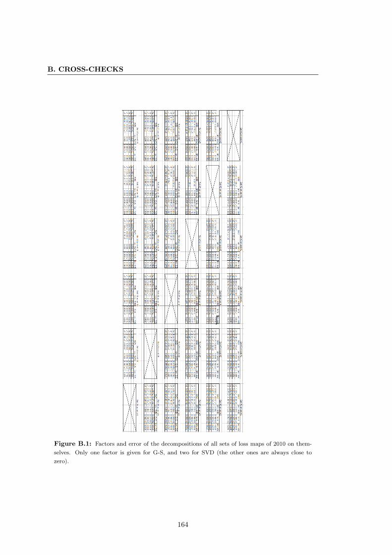
B. CROSS-CHECKS
Figure B.1: Factors and error of the decompositions of all sets of loss maps of 2010 on them-
selves. Only one factor is given for G-S, and two for SVD (the other ones are always close to
zero).
164

Figure B.2: Factors and error of the decompositions of all loss maps of 2011 on the average set
of selected loss maps used for decomposition of real data. Only one factor is given for G-S, and
two for SVD (the other ones are always close to zero).
165

B. CROSS-CHECKS
166
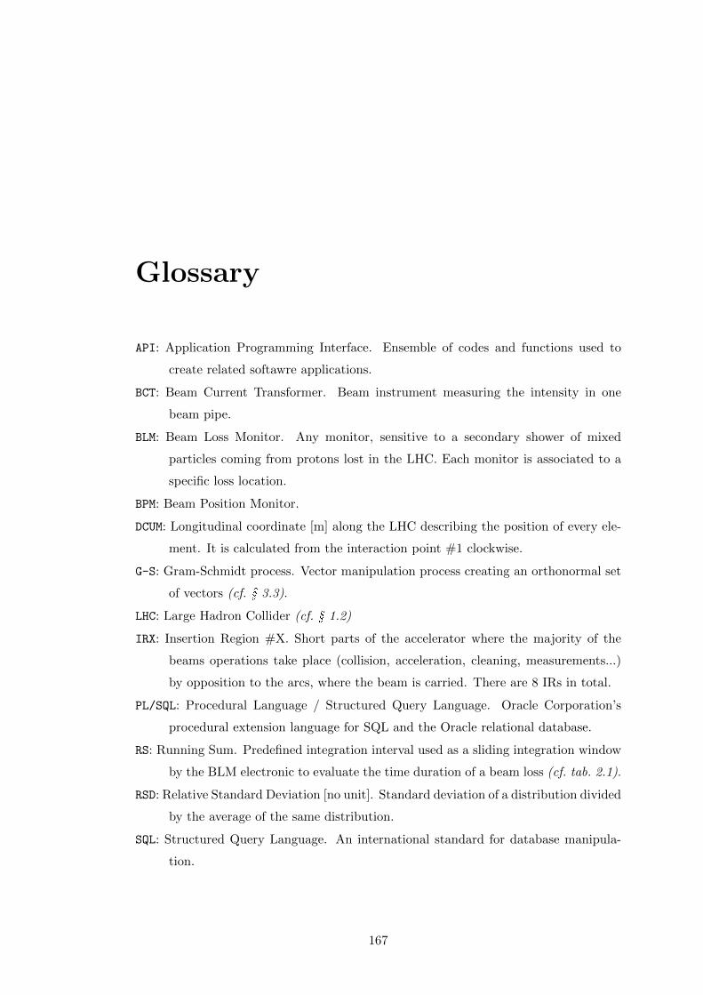
Glossary
API: Application Programming Interface. Ensemble of codes and functions used to
create related softawre applications.
BCT: Beam Current Transformer. Beam instrument measuring the intensity in one
beam pipe.
BLM: Beam Loss Monitor. Any monitor, sensitive to a secondary shower of mixed
particles coming from protons lost in the LHC. Each monitor is associated to a
specific loss location.
BPM: Beam Position Monitor.
DCUM: Longitudinal coordinate [m] along the LHC describing the position of every ele-
ment. It is calculated from the interaction point #1 clockwise.
G-S: Gram-Schmidt process. Vector manipulation process creating an orthonormal set
of vectors (cf. § 3.3).
LHC: Large Hadron Collider (cf. § 1.2)
IRX: Insertion Region #X. Short parts of the accelerator where the majority of the
beams operations take place (collision, acceleration, cleaning, measurements...)
by opposition to the arcs, where the beam is carried. There are 8 IRs in total.
PL/SQL: Procedural Language / Structured Query Language. Oracle Corporation’s
procedural extension language for SQL and the Oracle relational database.
RS: Running Sum. Predefined integration interval used as a sliding integration window
by the BLM electronic to evaluate the time duration of a beam loss (cf. tab. 2.1).
RSD: Relative Standard Deviation [no unit]. Standard deviation of a distribution divided
by the average of the same distribution.
SQL: Structured Query Language. An international standard for database manipula-
tion.
167

B. CROSS-CHECKS
SQL: Singular Value Decomposition. Matrix inversion technique used in this work
(cf. § 3.2).
TCP: Primary collimator. Element of the accelerator which is the closest to the particle
beam.
TCT: Tertiary collimator.
Timestamp: Association of a date and a time (with a precision of one second) corre-
sponding to one value in a database.
168
Bibliography
[1] “LHC Design Report”, CERN-2004-003-V-1. p 3
[2] E. B. Holzer, B. Dehning et al. “Beam Loss Monitoring for LHC Machine Protec-
tion”, proceedings, TIPP 2011. p 11
[3] R. Alemany, M. Lamont, S. Page, “LHC MODES”, Functional specification, 11-
2007, LHC-OP-ES-0005. p 8, 9
[4] B. Puccio, R. Schmidt, J. Wenninger “Beam interlocking strategy between the
LHC and its injector”, proceedings, ICALPECS 2005. p 11
[5] R. Assman et al., “The final collimation system for LHC”, CERN-LHC-Proj.-
Report-919, 2006. p 11, 13, 15, 16
[6] R. Bruce, R. Assmann, “Collimator settings in 2012”, presented at the LHC Ma-
chine Committee, 28/03/2012. p 14, 15
[7] Markus Stockner, “Beam Loss Calibration Studies for High Energy Proton Accel-
erators”. PhD thesis, CERN-THESIS-2008-099 . p 22
[8] A. Arauzo and C. Bovet, “Beam loss detection system in the arcs of the LHC”.
Technical Report, CERN-SL-2000-052 BI. p 22
[9] D. Kramer, “Design and Implementation of a Detector for High Flux Mixed Ra-
diation Fields”. PhD thesis, CERN-THESIS-2008-090. p 3, 23, 24
[10] C. Zamantzas, “The Real-Time Data Analysis and Decision System for Particle
Flux Detection in the LHC Accelerator at CERN”, CERN-thesis-2006-037. p 29
169

BIBLIOGRAPHY
[11] E. Nebot et al., “Handling of BLM abort thresholds in he LHC”, IPAC 2011,
WEPC170. p 29
[12] Todd Will, UW-La Crosse, “Introduction to the Singular Value Decomposition”
http://www.uwlax.edu/faculty/will/svd/index.html p 37
[13] B. Autin, Y. Marti, “Closed orbit correction of A.G. Machines using a small num-
ber of magnets”. Technical report, CERN-ISR-MA-73-17. p 43
[14] “LHC e-Logbook”, LHC operation group, BE-OP, CERN
https://ab-dep-op-elogbook.web.cern.ch/ab-dep-op-elogbook/elogbook/
eLogbook.php p 49
[15] “Horizontal and vertical blow-ups”, private communication with Daniel Wollmann,
BE-APB, CERN. p 49
[16] All available views, C. Roderick, BE–CO–DM, http://lhc-logging.web.cern.
ch/lhc-logging/software/public_data_access_views.jpg p 133, 135, 136
[17] LHC Logging Project, C. Roderick, BE–CO–DM, http://lhc-logging.web.
cern.ch/lhc-logging/software/default.htm p 133
[18] ConfigParser module, python documentation,
http://docs.python.org/library/configparser.html p 134
[19] TSQLServer, ROOT documentation,
http://root.cern.ch/root/html528/TSQLServer.html p 134, 135
[20] Logging Data Extraction Client, Command Line API, https://espace.cern.ch/
be-dep/CO/DM/CALS/other/CommandLineManual.pdf p 136
[21] TGraph, ROOT documentation, http://root.cern.ch/root/html528/TGraph.
html p 141
[22] shelve module, python documentation,
http://docs.python.org/library/shelve.html p 160
170