University of Alaska Anchorage

Society of Automotive Engineers

2015 Baja Team

ME A438 Fall 2014 Senior Design Report

Design Team Members:

Galen Baumgartner Devon Jones Jun Mendoza Valisa Hansen Elena Stutzer

Faculty Advisors:

Dr. Jeffrey Hoffman & Dr. Todd Petersen

Date: Friday, December 5, 2014

2

Report Contents

1.0 Introduction ............................................................................................................................... 4

1.1 Project Statement.............................................................................................................. 4

1.2 Project Scope .................................................................................................................... 5

2.0 Methods..................................................................................................................................... 5

2.1 Frame ..................................................................................................................................... 6

2.1.1 Material ........................................................................................................................... 7

2.1.2 Finite Element Analysis .................................................................................................. 8

2.1.3 Existing Testing ............................................................................................................ 11

2.1.4 Weight .......................................................................................................................... 14

2.1.5 Ergonomics ................................................................................................................... 15

2.2 Front Suspension and Steering ............................................................................................ 15

2.2.1 Design Parameters ........................................................................................................ 15

2.2.2 Impact Force ................................................................................................................. 16

2.2.3 Frontal Impact............................................................................................................... 17

2.2.4 Suspension Geometry ................................................................................................... 17

2.2.5 Simulation ..................................................................................................................... 19

2.2.6 Experiment.................................................................................................................... 20

2.3 Controls and Brakes Systems .............................................................................................. 22

2.3.1 Basis of Brake Design .................................................................................................. 23

2.3.2 Hydraulic Brake System ............................................................................................... 23

2.3.3 Pedal Design ................................................................................................................. 26

2.3.4 Gear Shifter Design ...................................................................................................... 28

2.4 Rear Suspension .................................................................................................................. 29

2.4.1 Design Criteria .............................................................................................................. 29

2.4.1 Suspension Type ........................................................................................................... 29

2.4.2 Finite Element Analysis ................................................................................................ 30

2.4.3 Trailing Arm ................................................................................................................. 31

2.4.4 Bearing Carrier ............................................................................................................. 31

2.4.5 Mounting Devices......................................................................................................... 31

3.0 Results ..................................................................................................................................... 32

3.1 Finalized Frame ................................................................................................................... 33

3

3.1.1 Frame Analysis Results ................................................................................................ 33

3.2 Front Suspension Study Results .......................................................................................... 42

3.2.1 Front Suspension Geometry ......................................................................................... 42

3.2.2 Finite Element Analysis ................................................................................................ 44

3.3 Control Systems Anlalysis .................................................................................................. 47

3.4 Rear Suspension Iterations .................................................................................................. 51

3.4.1 Bearing Carrier Results ................................................................................................ 52

3.4.2 Trailing-Arm Results .................................................................................................... 52

3.4.3 Mounting Device Results ............................................................................................. 53

4.0 Conclusion .............................................................................................................................. 55

5.0 References ............................................................................................................................... 55

6.0 Appendix A: Material Certification ........................................................................................ 56

6.1 Appendix B: Roll Cage Equivalency Calculations ................................................................. 57

4

1.0 Introduction

Baja SAE (Society of Automotive Engineers) is an international collegiate design

competition sponsored by the Society of Automotive Engineers. The competition is held every

year and presents engineering students with the challenge of designing a mechanical system and

implementing that design through the construction of an off-road vehicle. The 2015 Baja Car

will be the fifth car designed, assembled and raced by University of Alaska Anchorage (UAA)

engineering students in the Baja SAE annual competition.

This year, a complete redesign of the car was the primary focus of the Baja Team.

Improvement of five key systems, the chassis (frame), breaks, shifter, front suspension and rear

suspension, was the target of this redesign. These subsystem improvements were based on

assessment of the previous cars raced by UAA, as the ultimate goal of the 2015 UAA Baja Team

is to score within the top 20% upcoming Baja SAE competition.

Design was divided between sub-teams that focused on each of the five subsystems. Each

subsystem team worked with the group as a whole to meet mutual team goals. Each team

produced a SolidWorks model of its subsystem, which was then assembled into the model of the

entire car. This model allowed the Team to compile stress/strain data and improve upon the

design of the car as the project progressed. SolidWorks Simulation was used to perform finite

element analysis and motion analysis on the vehicle to optimize the performance and efficiency

of each component and subsystem.

1.1 Project Statement

The Society of Automotive Engineers hosts an annual design competition for engineering

students. The competition challenges participants to design and build an off-road vehicle. In May

2015, the Baja Team will race the fifth car designed and assembled by students in the UAA

College of Engineering.

This year, the car was to be redesigned using the experiences of the past four UAA Baja

Teams, as well as advising from the faculty and staff of the UAA College of Engineering. The

Team’s focus was primarily on the redesign of five key systems: the chassis (frame), breaks,

5

shifter, front suspension and rear suspension. The Team assessed the performance of the

previous UAA Baja SAE cars, placing the most emphasis on the car from last year (2014), to

define the particular strengths and weaknesses that needed to be addressed for each individual

subsystem. The 2015 Team improved these systems, identified as the car’s weakest components,

in order to design a more competitive vehicle.

1.2 Project Scope

The primary goal of the 2015 UAA Baja Team is to score within the top 20% at the May 27-

30, 2015 SAE Baja competition in Portland, Oregon. To accomplish this goal, the group was

divided into sub-teams.

The task of design was divided by subsystem. Each team had a primary focus: the frame,

front suspension, rear suspension, shifter and brakes. Individual teams closely followed the SAE

Baja competition guidelines as stated in the official rule handbook to maintain the car’s

eligibility for competition. The vehicle was also designed ergonomically such that it can

accommodate a variety of drivers, while still meeting all safety requirements. Thus, each sub-

team worked closely with the group as a whole in order to meet universal goals. This need for

cohesion provided group members with an opportunity to develop team skills, as well as apply

concepts from course work to real-life engineering obstacles. As a result, the Baja vehicle is a

project that lives beyond the classroom.

For this class, SolidWorks was utilized to create a model of the entire car and its components

that represented the design decisions of the Baja Team. This software’s finite element analysis

capabilities allowed the Team to collect stress/strain data and produce motion analyses. These

helped the team create strong and efficient components and catch potential fabrication issues.

Thus, the UAA Baja Team used the solid model built in SolidWorks to perfect the car before

preparing to move into the fabrication stage in the spring.

2.0 Methods

Each sub-team validated a proposed design for strength and durability, as well as other

qualities such as machinability, weight and cost effectiveness. The team considered material,

6

geometry and overall ergonomics to optimize components and maximize the performance of the

vehicle by addressing the qualities of each of its components. The use of finite element analysis

(FEA) was also an integral part of identifying potential system failures such that a design could

be improved upon and eventually perfected. For design analysis, the team utilized the finite

element analysis capabilities of SolidWorks.

FEA is a means of performing tests on a design without necessitating a physical prototype.

The process consists of a three-dimensional model of a design that has a specified material. This

model is then subjected to stresses and analyzed for results. FEA uses nodes, a system of points

distributed throughout the model, to create a grid called a mesh. This mesh allows conditions, in

this case stresses, at one node, beginning with nodes that have defined boundary conditions such

as a load, to assist in the calculation of the conditions in neighboring nodes. This numerical

process continues until conditions throughout the entire model have been defined. The mesh

density, how fine or coarse the mesh is, depends on the expected stress levels of a given region.

The finer the mesh, the more accurate the results of the test; the finer the mesh, however, the

longer the computational time of the program. Thus, it is important to only apply fine meshes in

regions of particular interest. Stress risers such as fillets and holes, detailed areas, corners, areas

that undergo high levels of stress, or previous points of failure are regions that are critical in

terms of design.

Finer meshes are also necessary in order to perform a mesh convergence study [1]. Mesh

convergence proves that a sufficient number of nodes were used to define the model. The

condition is reached through reducing the mesh size until the difference between one test and the

next is one percent or less. Convergence is crucial because it demonstrates the accuracy of results

obtained from FEA. In addition, data acquired through FEA studies must be compared to a

problem with a known solution, such as the analytical solution to a similar problem, numerical

solutions, or experimental data.

2.1 Frame

The most important feature of the vehicle is the highly engineered crash-absorption

component that safeguards the driver during an impact by dispersing the effect of forces imposed

7

on the vehicle more predictably. The frame is the primary structure of the Baja vehicle because

it is the groundwork into which all other subsystems are integrated for the ideal engineering

design. This year, the goals for the frame were lightweight, simple, solid, strong and safe. The

engineering processes geared towards meeting the goals for the frame are discussed in the

following sections.

2.1.1 Material

Material selection is an important part of the frame, as it is fundamental to select materials

that will result in the greatest performance. The SAE Baja 2015 regulations per Rule B8.3.12

require material properties of the frame to meet various design aspects, such as bending strength,

bending stiffness and carbon content [2]. Yield strength, machinability, weight, and cost are also

factors to consider. After careful consideration and assessment, 4130 normalized alloy steel

(Chromoly) was selected as the material for the frame. Complete specifications for the material

are provided in Appendix A.

Criteria for Frame Material Selection:

I. Bending Stiffness

In order to meet the SAE Baja 2015 regulations, material selections must be compared with 1018

carbon steel as a reference [2]. The 4130 carbon steel met the guideline with a bending stiffness

of 3,633 N-m2, as detailed in Appendix B. The bending stiffness is calculated using Equation

2.1a for bending stiffness and Equation 2.1b for second area moment of inertia for the circular

steel tubing, I, where do and di represent the outer and inner diameters of the tubing, respectively.

(2.1a)

(2.1b)

II. Bending Strength

According to the SAE Baja 2015 regulations, the bending strength must be equal to the minimum

bending strength of 1018 low carbon steel [2]. The bending strength of 485,648 N-mm for 4130

carbon steel is calculated by equation 2.1c, where Sy is the yield strength, I is the second area

moment of inertia and c is the distance from the neutral axis (or radius).

(2.1c)

8

III. Yield Strength

Although it is not required by the 2015 Baja SAE rulebook, the yield strength of 435 MPa was

also an appealing attribute of the 4130 carbon steel, especially compared to the 365 MPa of plain

1018 carbon steel.

IV. Carbon Content

The required carbon content for the steel alloy chosen must be at least 0.18% and 4130 carbon

steel met the requirement with 0.28%-0.33% (2015 Baja SAE, pg. 27).

V. Machinability

Machinability refers to the ability for a metal to be worked with little effort for a presentable

result. Some measures of machinability are the degree of wear inflicted on tools used to machine

the metal, the required power consumption of the tool and the material’s hardness. There are no

2015 Baja SAE regulations governing this quality, however, the 4130 carbon steel does not

prove difficult to manipulate.

VI. Weight

The weight of the material is also an important aspect in the criteria for frame material selection,

as it is essential to have a light frame in order to achieve maximum performance. Due to the size

selections for the 4130 carbon steel, the weight of the vehicle can be lessened.

VII. Cost

The reference material is 1018 low carbon steel as determined by the SAE regulations. The 4130

carbon steel offers a comparable price, but also the bonus of superior material properties.

2.1.2 Finite Element Analysis

To validate the integrity of the frame, the design team used the finite element analysis (FEA)

package in SolidWorks. To simulate potential impact scenarios of the Baja vehicle during the

race, forces were applied to specific locations on the car. The following is a list of impacts the

team considered:

Frontal impact

Nose dive impact

Front shock/suspension impact

9

Side/T-bone impact

Top roll impact

Side roll/tipping impact

Skid plate impact

Rear shock impact

Rear impact

Details governing the setup of each scenario in the FEA package are outlined as follows.

I. Frontal Impact

Based on the momentum of the moving vehicle, the force of the car impacting a solid surface

was modeled using the following base equation:

(2.1d)

where is the force applied in lbm, p is the momentum of the car and is the duration of

the collision. Momentum is equal to the mass multiplied by the velocity, v, of the car in ft/s.

Thus, the force applied in lbf was calculated using the equation:

(2.1e)

where w is the weight of the car in lbf and g is the acceleration due to gravity in ft/s2. The total

weight of the car was taken to be 650 lbf, which includes a 400 lbf car, a 225 lbf driver and

25 lbf of mud from the competition track. The length of the collision was estimated to be 0.09 s,

the velocity 16 mph (22 ft/s), and the acceleration of gravity 32.17 ft/s2. In this manner, the

frontal collision force was calculated to be 5,300 lbf. This force was divided equally between the

four front members of the vehicle, resulting in a stress of 1325 lbf applied to each member.

II. Nose Dive Impact

The force on the vehicle resulting from a nose dive was calculated using equation 2.1e, where the

velocity was equal to the following:

√ (2.1f)

where h is the height from which the car falls, which was estimated at 3 ft, and all other variables

remained the same. The resulting force was 3100 lbf, which was applied to the lower front

member.

10

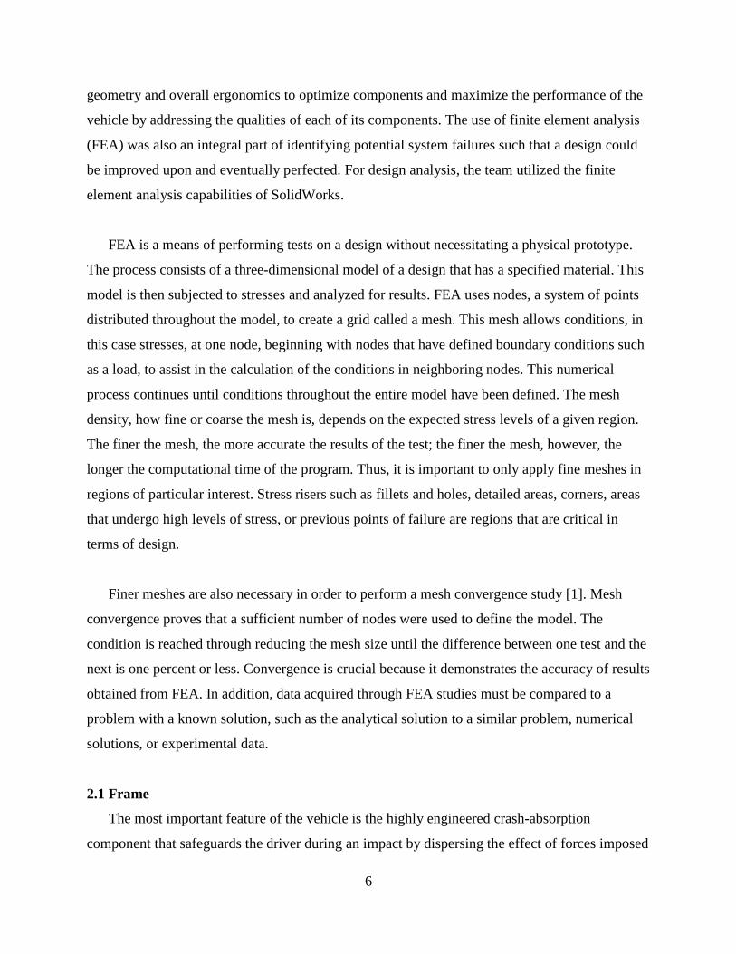
III. Front Shock Impact

The impact due to complete actuation of the front shock was calculated to be 795 lbf acting 42

degrees from horizontal. The vertical component of this resultant force was tabulated at 532 lbf,

and the horizontal component 591 lbf. The vertical and horizontal forces were applied to the

frame model at the location of the shock mount, with the vertical force acting upwards and the

horizontal component acting in a direction pointing towards the center of the vehicle.

IV. Side Impact

A force of 890 lbf was applied normal to the side impact member (SIM) next to the driver in

order to simulate a situation where the frame is T-boned by another car. The force was calculated

using equation 2.1e, but the velocity was taken to be only 3 mph (4.4 ft/s), as it was deemed

unlikely that another car would be going at maximum speed when impacting another vehicle

during competition. The chosen velocity was meant to represent another car grazing past in a

competitive race around a corner or another similar scenario. Thus, the impact time was

increased to 0.1 s.

V. Top Roll and Side Roll/Tipping Impacts

If the frame were to experience a roll or tip onto the upper roll hoop (RH) members, the

maximum force that could be experienced is the total weight of the car. Therefore, the roll

scenarios were modeled with applied forced of 650 lbf to the upper roll hoop members.

VI. Skid Plate Impact

The force resulting from the rear shocks being unable to fully absorb an impact before the skid

plate protecting the transaxle hits an object was approximated as a drop sustained from 0.5 feet

using Equations 2.1e and 2.1f. The time of the impact was taken to be 0.1 s, as the impact could

be somewhat slowed by the shocks. The impact force was thus found to be 1150 lbf. This force

was split equally between the first two segments of the skid plate, creating an applied force of

573 lbf per segment.

When attempting to pass over an unduly large object, the skid plate may also sustain an impact.

Assuming a driver would be aware of large obstacles and slow down accordingly, the situation

11

was modeled as an impact at 3 mph (4.4 ft/s), as the side impact previously discussed. Thus, a

force of 890 lbf was applied parallel to the first segment of skid plate predicted to bear the brunt

of the impact.

VII. Rear Shock Impact

The impact due to complete actuation of the rear shock was calculated to be 795 lbf acting 42

degrees from horizontal. The vertical component of this resultant force was tabulated at 532 lbf,

and the horizontal component 591 lbf. The vertical and horizontal forces were applied to the

frame model at the location of the shock mount, with the vertical force acting upwards and the

horizontal component acting in a direction pointing towards the center of the vehicle.

VIII. Rear Impact

An assumption was made that the vehicle would not back into anything at any significant speed,

thus the rear impact was meant to simulate the car being rear-ended by another vehicle. In

addition, assumptions had to be made about the nature of the incident like those made in regards

to the side impact. Here, it was assumed that the collision would occur at approximately half the

speed of the frontal collision, which was calculated at the car’s full 16 mph. Thus, the force of

the impact was found to be 2650 lbf, half the force of the frontal impact. This force was

distributed equally between the lower three members at the back of the vehicle, resulting in an

applied force of 880 lbf per member.

2.1.3 Existing Testing

The primary objective of the frame team is to incorporate all of the subsystems into one

cohesive vehicle and to ensure safe operability. To reach optimal results, FEA studies were

performed in SolidWorks. In order to validate these FEA studies, an existing study from the

2014 Baja Team that was conducted on the 2013 Baja vehicle was used, as the Team found that

it is not feasible to perform a mesh convergence study when using Weldments in SolidWorks [3].

The use of physical test results validated the FEA results by comparing the deflection of the

actual 2013 frame and deflection tabulated in a SolidWorks Simulation. The following Figures

12

2.1a and 2.1b show the locations of the applied forces and the test set-up used by the 2014 Baja

Team.

Figure 2.1a. 2013 Baja vehicle frame test set-up [3]

Figure 2.1b. Location of the applied forces [3]

The test procedures for the physical test performed by the 2014 Baja Team were as follows:

The 2013 frame was secured to the custom made steel frame with the use of chains

The Load Cell model number RL20000B-2k was secured to the frame member and the

come-along (see Figures 2.1a and 2.1b on the previous page)

Measurements between frame members were taken (see column (2) in Table 2.1 below)

The magnitude and angle of the applied force was recorded

13

Measurements of the frame were taken while the frame was under external load to

determine maximum deflection (see column (3) in Table 2.1)

After the force was released, the measurements between the frame members were

recorded a final time (see column (5) in Table 2.1)

The above steps were repeated for two more locations

Table 2.1 below illustrates the results yielded by the deflection test compared to the FEA

simulation conducted. Column (1) is the path of the measurement (see figure 2.1c below).

Column (2) and (5) consist of the actual measurements between frame members before and after

the force was applied. Column (3) contains the measurements for when the frame was under the

external load. The following experiment was replicated in SolidWorks and the measurements

yielded from that simulation are present in column (4).

Table 2.1. Deflection Measurement [3]

Dimension

(1)

Initial (in)

(2)

Test (in)

(3)

FEA (in)

(4)

Final (in)

(5)

Percent Error

(6)

D1 50.8 50.9 51.8 50.8 1.7

D2 40.0 40.1 41.2 40.0 2.6

D3 51.0 51.3 47.7 50.8 7.5

D4 56.5 57.0 54.6 56.8 4.4

D5 57.0 57.0 54.8 56.8 4.1

D6 40.0 39.5 38.0 40.0 4.0

D7 34.1 34.1 35.3 34.1 3.4

D8 33.9 33.9 32.2 33.9 5.4

Figure 2.1c. Dimension measurement legend [3]

14

After applying the external load that varied between 700-850 lbf, the maximum deflection

achieved was 0.625 inches in compression and there was no significant plastic deformation. The

results achieved are acceptable because the minimum required driver clearance is 3 inches,

which was not compromised when the frame deflected. Moreover, the small percent error

between the physical test and the FEA simulation is acceptable validation of the finite element

analysis tests in SolidWorks [3].

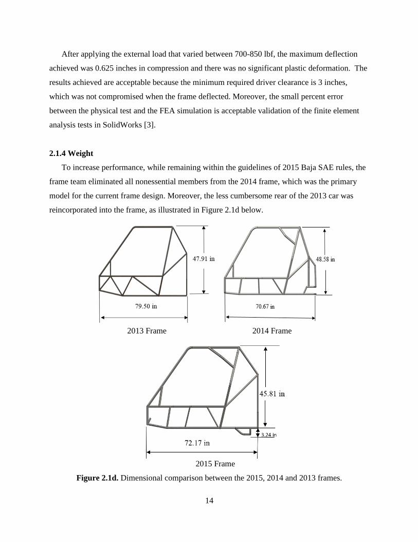
2.1.4 Weight

To increase performance, while remaining within the guidelines of 2015 Baja SAE rules, the

frame team eliminated all nonessential members from the 2014 frame, which was the primary

model for the current frame design. Moreover, the less cumbersome rear of the 2013 car was

reincorporated into the frame, as illustrated in Figure 2.1d below.

2013 Frame 2014 Frame

2015 Frame

Figure 2.1d. Dimensional comparison between the 2015, 2014 and 2013 frames.

15

As shown, this rear end frame design is more streamline and is expected to result in a decrease in

the overall weight of the car and to a lesser extent the size of the vehicle. With unnecessary

tubing removed and a slightly shortened vehicle, the 2015 car is smaller overall compared to the

2013 and 2014 UAA Baja vehicles.

2.1.5 Ergonomics

The 2015 frame was designed to accommodate a 5-foot and 6-foot tall driver, as B1.3 of the

2015 Baja SAE rulebook requires the design of a “commercial” product that can accommodate a

5th

percentile female as well as a 95th

percentile male [2]. Thus, the roll cage was designed to be

tall enough to seat the six-foot driver, and the chassis was made to accommodate the breadth of

this driver. Moreover, the harness bar must be placed such that the harness fits snugly and in

accordance with regulation B10.2.1 of the Baja SAE 2015 rulebook, which states that the harness

shoulder straps be mounted no higher than vertical shoulder height (measured based on the

smallest driver), and no lower than 4 inches below the shoulder (measured based on the tallest

driver) [2]. Such considerations were taken into account throughout the design process.

2.2 Front Suspension and Steering

The steering and suspension are vital to the Baja vehicle operability. The systems must be

carefully tuned to respond to the driver and the terrain during fast-paced competition. The

components must also be robust enough to withstand the unforgiving off-road terrain the vehicle

will encounter. The following section details the design of both the front suspension and steering.

2.2.1 Design Parameters

To establish design parameters for the suspension and steering assembly, some assumptions

about vehicle and driver weight were made. Vehicle weight was approximated using the known

weight of the 2014 vehicle of 400 lbs. This is a valid assumption considering this year’s car is

going to be of similar size and constructed of similar materials. The maximum weight of the

drivers on the current Baja Team is 225 lbs. Due to the conditions in Oregon, the vehicle is also

expected to accumulate 25 lbs of mud and debris during the race. Combined, this makes up a

total weight of 650lbs.

16

2.2.2 Impact Force

To estimate the vertical forces acting on the A-arms, video footage from previous

competitions was analyzed. The maximum vertical drop a vehicle made to a flat surface was

estimated to be three feet, as illustrated in Figure 2.2a below.

Figure 2.2a. Illustration of a 3ft drop to a flat surface.

This simulation focuses on the forces applied vertically through the suspension; therefore the

kinetic energy of the vehicle as it moves forward is ignored. The potential energy of a falling

object is equal to the kinetic energy right before it impacts the ground as shown in equation 2.2a.

(2.2a)

In this equation, m is the mass of the vehicle, g is the acceleration due to gravity, h is the

vertical drop height, and v is the velocity of the vehicle before impact.

Kinetic energy “is a measure of a particle’s capacity to do work” [4]. This means that

the kinetic energy of the falling vehicle right before impact is the amount of work the

suspension needs to be able to withstand. Work can be defined as:

(2.2b)

W is the amount of work, F is the force applied and △s is the 10-inch suspension travel plus a 1-

inch compression of the tires. Because the kinetic energy before impact is equal to the potential

energy of the vehicle at 3 feet, we can set the potential energy and work required equal, and

derive following equation:

(2.2c)

17

The vehicle will land on all 4 tires simultaneously; therefore the force can be multiplied by a

factor of 0.25 to divide the force equally between the tires. To ensure the suspension will

withstand any scenario it may encounter on the track, a safety factor of 2 was also used.

(2.2d)

By using Equation 2.2d the force applied at each tire resulting from a 3 foot drop was calculated

to be 1060 lbf.

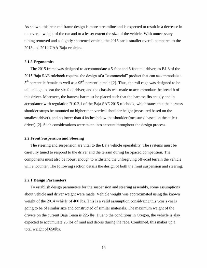
2.2.3 Frontal Impact

The front suspension needs to withstand the same impact that the frame will likely see. To

establish a value for a frontal impact, the method outlined in section 2.1.2 and equation 2.1e was

again used. A 16 mph collision also equates to a vertical drop height of 8.5 ft, which is well

above any “nose dive” the vehicle will encounter. Figure 2.2b below illustrates this scenario.

Figure 2.2b. Frontal impact scenario.

The total force applied was calculated to be 5500 lbf. Multiplying by a safety factor of 2 and

dividing the force equally between the four A-arms resulted in a force of 2750 lbf per A-arm.

2.2.4 Suspension Geometry

The A-arm type front suspension of the 2013 and 2014 Baja vehicles was able to withstand

the extreme terrain in both Washington and Texas. This provided a sound suspension design

foundation off of which to build. The overall goal for 2015 is to improve the suspension

geometry in terms of maneuverability without sacrificing durability.

18

With the strengths of previous vehicles in mind, the 2015 design continues to use Polaris

knuckles and ball joints. This year’s design also uses 7/16th

inch rod ends as mounting points.

The rod ends add strength and also allow the suspension to be fine-tuned after assembly.

The major weakness identified in the 2014 design was excessive bump steer. Bump steer is

caused when the tires either turn out or in as the suspension travels up and down. This put added

stress on the tie rods and ultimately led to failure. To minimize bump steer, the motion of the

suspension was closely examined in SolidWorks while manually running the suspension through

its full travel. It was found that by keeping the tie rods and A-arms parallel and of similar length,

bump steer could be almost completely eliminated.

To improve maneuverability, the main area of concern is the steering geometry. When a

vehicle makes a turn, the two front tires must follow different radii [5]. For the vehicle to follow

the path around a curve without the tires slipping, the inside tire must turn sharper to follow the

smaller radius. This arrangement, known as Ackerman steering geometry, is shown in Figure

2.2c. To incorporate Ackerman steering geometry into the design, a line that intersects the

steering arm and steering axis should also intersect the rear axle near the midpoint as shown in

Figure 2.2d.

Figure 2.2c. Ackerman steering [6]. Figure 2.2d. Steering axis and rear axle .

intersection [6].

The geometry of the Polaris knuckles required that they be rotated 180 degrees and used on

the opposite side of the vehicle to achieve the desired effect. This had the added benefit of

moving the steering rack to the front of the vehicle, out of the way of the driver’s feet.

19

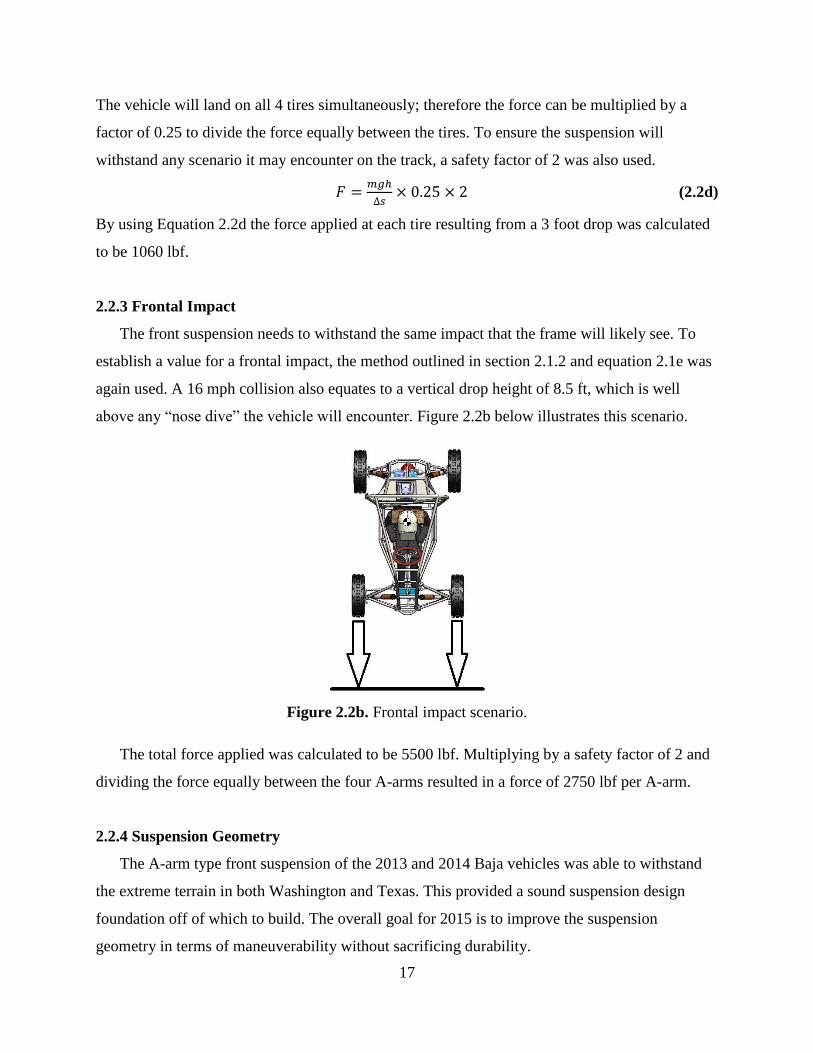
Other important design considerations in the steering system of an off-road vehicle are the

caster angle and camber angle. Below, Figure 2.2e shows the definition of caster angle and

Figure 2.2f shows the camber angle.

Figure 2.2e. Caster angle [7]. Figure 2.2f. Camber angle [7].

The caster angle is important for the stability of the vehicle. A positive camber angle (as

shown in Figure 2.2e) is beneficial as it helps the wheels auto-center if they are diverted by an

obstacle. A negative caster angle would do the opposite and pull the wheels away from center

when disturbed. A positive caster angle also aids in cornering by adding camber angle as the car

is steered away from center. If the caster angle is increased by too much it makes the vehicle less

responsive to steering input. A caster angle of 10 degrees was chosen to increase stability

without decreasing responsiveness.

The camber angle is important for the performance of the vehicle in high speed turns. A

negative camber angle places the tire at a better angle to the road, transmitting the forces through

the vertical plane of the tire rather than through a shear force across it. A camber angle of

5 degrees was chosen as a base point. The ball joints on the A-arms permit adjusting camber

angle after assembly.

2.2.5 Simulation

Once the necessary geometry was established the components were modeled using

SolidWorks. Because of the complexities of three-dimensional connections in the final assembly,

a second simplified model was created to study the kinematics of the system. This simplified

20

model is shown in Figures 2.2g and 2.2h. Every major component was then analyzed using FEA

in SolidWorks Simulation. The maximum predicted forces calculated in the Impact Force section

were applied to the components. If the maximum Von Mises stress was above the yield strength

of the material, the part was redesigned to reduce the overall stress. A convergence study was

also performed with every FEA study. A percent difference in displacement of less than 1% for a

change in mesh size was considered an acceptable result.

Figure 2.2g Simplified suspension model.

Figure 2.2h Simplified suspension model running through full suspension travel.

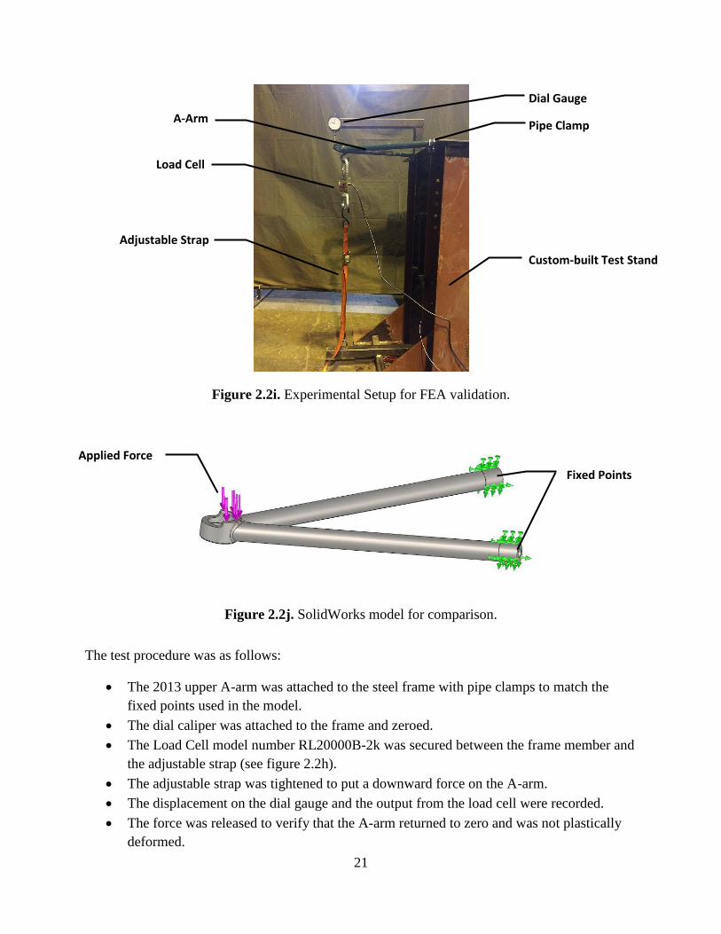
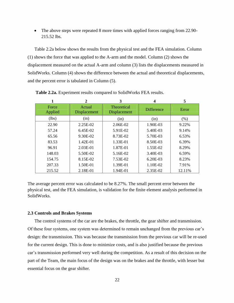
2.2.6 Experiment

The FEA results were validated experimentally by comparing the displacements of the actual

2013 upper A-arm to the theoretical displacements calculated in a SolidWorks Simulation.

Figure 2.2i at the top of the following page shows the experimental setup and Figure 2.2j shows

the corresponding SolidWorks model under the same load.

21

Figure 2.2i. Experimental Setup for FEA validation.

Figure 2.2j. SolidWorks model for comparison.

The test procedure was as follows:

The 2013 upper A-arm was attached to the steel frame with pipe clamps to match the

fixed points used in the model.

The dial caliper was attached to the frame and zeroed.

The Load Cell model number RL20000B-2k was secured between the frame member and

the adjustable strap (see figure 2.2h).

The adjustable strap was tightened to put a downward force on the A-arm.

The displacement on the dial gauge and the output from the load cell were recorded.

The force was released to verify that the A-arm returned to zero and was not plastically

deformed.

Custom-built Test Stand

Dial Gauge

Adjustable Strap

Load Cell

Pipe Clamp A-Arm

Fixed Points

Applied Force

22

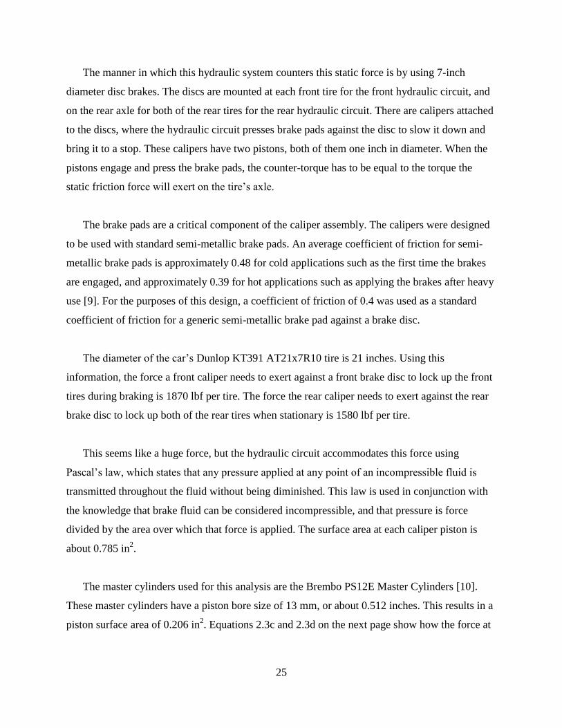
The above steps were repeated 8 more times with applied forces ranging from 22.90-

215.52 lbs.

Table 2.2a below shows the results from the physical test and the FEA simulation. Column

(1) shows the force that was applied to the A-arm and the model. Column (2) shows the

displacement measured on the actual A-arm and column (3) lists the displacements measured in

SolidWorks. Column (4) shows the difference between the actual and theoretical displacements,

and the percent error is tabulated in Column (5).

Table 2.2a. Experiment results compared to SolidWorks FEA results.

1 2 3 4 5

Force

Applied

Actual

Displacement

Theoretical

Displacement Difference Error

(lbs) (in) (in) (in) (%)

22.90 2.25E-02 2.06E-02 1.90E-03 9.22%

57.24 6.45E-02 5.91E-02 5.40E-03 9.14%

65.56 9.30E-02 8.73E-02 5.70E-03 6.53%

83.53 1.42E-01 1.33E-01 8.50E-03 6.39%

96.91 2.03E-01 1.87E-01 1.55E-02 8.29%

148.03 5.50E-02 5.16E-02 3.40E-03 6.59%

154.75 8.15E-02 7.53E-02 6.20E-03 8.23%

207.33 1.50E-01 1.39E-01 1.10E-02 7.91%

215.52 2.18E-01 1.94E-01 2.35E-02 12.11%

The average percent error was calculated to be 8.27%. The small percent error between the

physical test, and the FEA simulation, is validation for the finite element analysis performed in

SolidWorks.

2.3 Controls and Brakes Systems

The control systems of the car are the brakes, the throttle, the gear shifter and transmission.

Of these four systems, one system was determined to remain unchanged from the previous car’s

design: the transmission. This was because the transmission from the previous car will be re-used

for the current design. This is done to minimize costs, and is also justified because the previous

car’s transmission performed very well during the competition. As a result of this decision on the

part of the Team, the main focus of the design was on the brakes and the throttle, with lesser but

essential focus on the gear shifter.

23

2.3.1 Basis of Brake Design

The 2015 Baja SAE competition rules state that all four tires must “lock up” when the brake

pedal is actuated, preventing them from moving [2]. Not only does this need to be accomplished

when the car is in motion, but it also needs to be accomplished when the car is stationary, so that

if the car is pushed when it is not moving it does not roll away from its initial position. A

technical inspection is performed at the Baja SAE competition to determine if this criterion is

met.

2.3.2 Hydraulic Brake System

The hydraulic brakes are actuated by using a mechanical advantage called a pedal ratio,

which is defined as the ratio of the distance between the application of the foot’s force on the

pedal and the hinge, and the distance between the application of the pedal’s force on the master

cylinders and the hinge. Equation 2.3a below shows this relationship:

(2.3a)

The purpose of a pedal ratio is to multiply the force applied by the foot to pressurize the

brake system lines. The higher the ratio, the more a foot’s force is multiplied when applied to the

brake pedal, and the more hydraulic pressure the brake system exerts on the tires of the car,

locking them up and bringing the car to a halt. Thus, it was essential that the Team choose an

appropriate pedal ratio.

The Team also considered how large the force applied to the pedal should be in order to

adequately pressurize both the front and rear hydraulic circuits. This was done by first

considering how much force would be needed to lock the tires. Thus, the Team looked at the

static friction force applied to the tires.

Attempting to accurately model the friction coefficient of a tire in an off-road scenario is

very difficult, since off-road tires are not modeled against friction itself. The tire treads and how

they deform under use is a far more significant factor than the friction coefficient between the

tire and the road, especially in muddy or sandy conditions. However, it is known that the more

the tire grips the road surface, the more force the brake system needs to exert on the tires in order

24

to lock the tires and bring the car to a stop. Thus, it is easier, although more conservative, to

consider the maximum possible friction coefficient between the tire and various road surfaces,

and use that number to model the maximum force required to bring the car to a halt. The

maximum static friction coefficient is 1 for a dry tire on a dry road, but only 0.9 for rubber on

asphalt [8]. Since 1 is the larger number, it was used for this analysis.

Statically, the tires support the entire weight of the car between them. This makes calculating

the static friction force the brake system needs to overcome in order to stop each tire a simple

matter using the following equation:

Ff = μsN (2.3b)

where μs is the frictional coefficient of 1, and N is the normal force acting on one tire as a result

of supporting the weight of the car. The normal force is equal in magnitude to the weight of the

car that each tire supports, as the calculation is done on a per tire basis.

The weight supported by each tire, however, is not equal. In order to account for this

incongruity, two breaking scenarios were considered. The first scenario accounts for when the

brakes are fully engaged and a portion of the car’s weight transfers onto the front tires. As a

result, the front tires take more weight during braking. Alternately, the second scenario accounts

for a stationary car where more weight is placed on the rear tires. Last year’s design had a

stationary weight distribution of 40% to the front tires, and 60% to the rear tires. The design’s

brakes were made to handle a 67% to 33% front-to-rear braking force distribution, in order to

account for the dynamic weight transfer. For the purposes of this calculation, a more

conservative 70% to 30% front-to-rear braking force distribution was used.

Assuming a conservative weight of 710 lbf for the car and driver resulted in a static friction

force of 249 lbf for each front tire, and 107 lbf for each rear tire. The brake system needs to

overcome this force in order to lock the tires and prevent them from moving when the vehicle is

in motion. When stationary, however, the weight bias was increased for the rear brakes, which

resulted in 210 lbf for each rear tire and 142 lbf for each front tire. These calculations gave a

maximum weight of 249 lbf for each front tire, and 210 lbf for each rear tire.

25

The manner in which this hydraulic system counters this static force is by using 7-inch

diameter disc brakes. The discs are mounted at each front tire for the front hydraulic circuit, and

on the rear axle for both of the rear tires for the rear hydraulic circuit. There are calipers attached

to the discs, where the hydraulic circuit presses brake pads against the disc to slow it down and

bring it to a stop. These calipers have two pistons, both of them one inch in diameter. When the

pistons engage and press the brake pads, the counter-torque has to be equal to the torque the

static friction force will exert on the tire’s axle.

The brake pads are a critical component of the caliper assembly. The calipers were designed

to be used with standard semi-metallic brake pads. An average coefficient of friction for semi-

metallic brake pads is approximately 0.48 for cold applications such as the first time the brakes

are engaged, and approximately 0.39 for hot applications such as applying the brakes after heavy

use [9]. For the purposes of this design, a coefficient of friction of 0.4 was used as a standard

coefficient of friction for a generic semi-metallic brake pad against a brake disc.

The diameter of the car’s Dunlop KT391 AT21x7R10 tire is 21 inches. Using this

information, the force a front caliper needs to exert against a front brake disc to lock up the front

tires during braking is 1870 lbf per tire. The force the rear caliper needs to exert against the rear

brake disc to lock up both of the rear tires when stationary is 1580 lbf per tire.

This seems like a huge force, but the hydraulic circuit accommodates this force using

Pascal’s law, which states that any pressure applied at any point of an incompressible fluid is

transmitted throughout the fluid without being diminished. This law is used in conjunction with

the knowledge that brake fluid can be considered incompressible, and that pressure is force

divided by the area over which that force is applied. The surface area at each caliper piston is

about 0.785 in2.

The master cylinders used for this analysis are the Brembo PS12E Master Cylinders [10].

These master cylinders have a piston bore size of 13 mm, or about 0.512 inches. This results in a

piston surface area of 0.206 in2. Equations 2.3c and 2.3d on the next page show how the force at

26

each master cylinder is related to the force at each caliper (at the front circuit and rear circuit,

respectively):

(2.3c)

(2.3d)

where FMC is the force on the master cylinder, FC is the force on the caliper, AMC is the area of

the master cylinder and AC is the area of the caliper.

Using this information, the force that needs to be applied at the master cylinder for the front

hydraulic circuit is about 245 lbf, and the force that needs to be applied at the master cylinder for

the rear hydraulic circuit is about 207 lb. This combined with a pedal ratio of 6 as per Equation

2.3a results in a required total pedal force of around 76 lbf, distributed between both hydraulic

circuits.

As described, the force required for each circuit is different. If the required pedal force of

76 lbf were applied equally to both circuits, then the front hydraulic circuit would not receive the

correct amount of force necessary to lock up the front tires. To compensate, the Team chose to

use a balance bar in the design.

The purpose of the balance bar is to re-distribute the forces acting on the master cylinders, so

that the master cylinder with the higher requirement receives adequate pressure for the system

without over-pressurizing the other master cylinder with the lower requirement. The balance bar

re-distributes these forces without increasing the required pedal force. However, installing a

balance bar requires minute adjustments until the proper brake state is found, and this is not

something that can be determined before construction [11].

2.3.3 Pedal Design

This year’s design re-uses the same brake discs and hydraulic circuits as last year’s design,

since those components are fully functional; the pedal, however, shall be constructed to a pedal

ratio of 6, which is an increase from last year’s design that used a pedal ratio of 5. To

accommodate for this larger pedal ratio, both the gas and the brake pedals will be mounted onto

27

brackets welded to the upper portion of the “nose” of the frame assembly, where the pedals will

hang down.

The force required to actuate the brake pedal is not the force that the pedals are designed to

withstand. According to research conducted by NASA, and also considering the cramped

conditions of the driver, the 5th percentile strength of an adult male leg with a thigh angle up

from level of approximately 33° to 36°, will have a maximum pushing strength of 1300 N, or

292 lbf [12]. According to the same research, a female’s lower extremities, which include the

various leg muscles, will be 85% to 55% the strength of a similar male’s lower extremities. This

gives upper and lower female leg strength at 33° to 36° maximums of 248 lbf and 160.6 lbf,

respectively. To be conservative and accommodate the maximum amount of force that any driver

could exert on the pedal, the pedal was designed to withstand 300 lbf of foot force on the pedal

face.

Solid models of the pedal assembly were made in SolidWorks in order to perform FEA and

test the design under loading. As a result of performing this analysis, which identified the

maximum stress state of the pedal assembly, the type of material the pedal assembly components

will be made of was determined.

In addition to strength, adjustability of the pedals was a significant concern as well. An

ergonomic design that accommodates a broad range of drivers is essential. Leg length differs and

affects performance if not taken into account. To compensate, the pedals were designed to be

adjustable, with a forward and a rear position. Thus, a driver with shorter legs can bring the

pedals closer, and a driver with longer legs can set the pedals farther away.

For ease of use, both the gas and the brake pedals were designed with a spring return so that

they naturally return to a neutral position after taking the foot off of each pedal. They were also

designed so that it is very difficult for the toes to come into contact with the pedal arm, as such

contact could potentially divert force to an undesirable spot on the pedals.

28

The gas pedal incorporates a throttle linkage to create a large throttle cable pull for a small

pedal movement. Mechanical stops attached to the frame were designed to prevent the throttle

cable from pulling too much and possibly breaking. There will be a linkage set for each gas pedal

position, to compensate for the changes in throttle movement as a result of adjusting the gas

pedal position.

Constructability was also considered during the design process. After consulting with the

University’s machinist, Corbin Rowe, multiple times [13], a design was decided upon that would

match the design criteria and be simple to construct, given the correct materials and welding

procedures. This design also repurposed other parts from previous car designs in an attempt to be

economic and simple.

2.3.4 Gear Shifter Design

The car shifts between two active gears, forward and reverse, with a neutral position in

between these gears. This is accomplished with a cable that is attached to the transmission on

one end, and the gear shifter handle on the other end. The gear shifter is required to have a

mechanical locking system that prevents the shifter from inadvertently changing position while

driving.

According to research from NASA, the maximum push and pull strengths of a right arm with

the elbow locked at a 90° angle with the center line of the body, which is how the driver’s arms

are restrained while in the safety harness of the car, are 36 lbf and 37 lbf, respectively [12]. The

shifter was designed to withstand a force of 40 lbf for both push and pull; this amount of force,

however, will only be a concern when the shifter assembly is in the locked position.

After consulting with the machinist, Corbin Rowe, a design that incorporates an internal

locking mechanism into the shifter handle was created [13]. This design also includes a spring to

return the locking pin to a locked position. The reason for the locking mechanism being internal

is to prevent the mechanism from being clogged with dirt or mud, which makes operating the

gear shifter much more difficult for the driver. Thus, ease of use was a primary design

consideration for the shifter.

29

2.4 Rear Suspension

Suspension is essential the success at the Baja SAE competition, as an off-road vehicle is

expected to navigate rough terrain. The following section highlights the design of the trailing-

arm suspension.

2.4.1 Design Criteria

The goal of the 2015 Baja team was to design a car with optimized suspension that could

withstand various terrain. Thus, the Team developed the follow list of criteria essential to

designing a rear suspension system suitable for the competition:

Choose a suspension type that minimizes stresses on internal suspension members (A-

arms, trailing-arms), yet accommodates the geometries necessary for reactive suspension.

Create a lightweight design.

Improve access to motor and transmission.

Base material selection on mitigation of fractures.

Reuse the Fox Float shocks from the previous vehicle.

2.4.1 Suspension Type

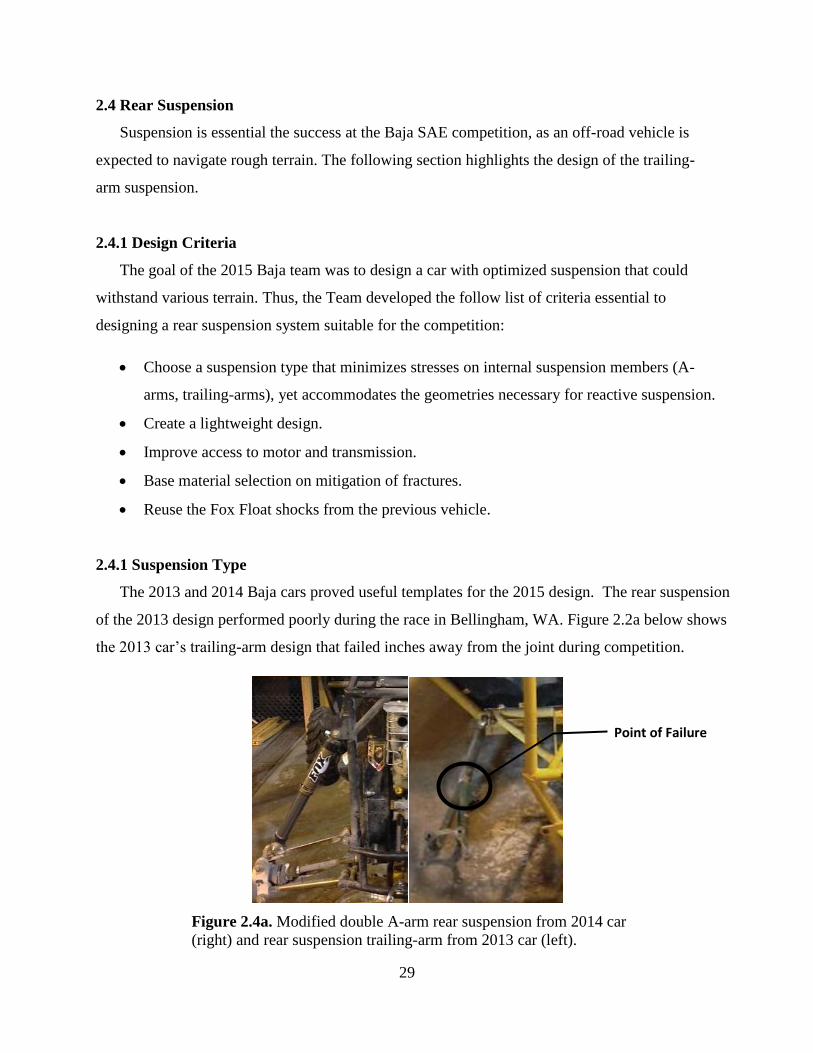
The 2013 and 2014 Baja cars proved useful templates for the 2015 design. The rear suspension

of the 2013 design performed poorly during the race in Bellingham, WA. Figure 2.2a below shows

the 2013 car’s trailing-arm design that failed inches away from the joint during competition.

Figure 2.4a. Modified double A-arm rear suspension from 2014 car

(right) and rear suspension trailing-arm from 2013 car (left).

Point of Failure

30

The 2014 Baja Team chose a modified double A-arm design for their rear suspension, as also

shown in Figure 2.2a. Unfortunately, this design concept remains untested, as other members of

the vehicle failed during the competition in El Paso, TX.

Thus, based on assessment of the various types of suspensions that the UAA Baja Team has

used in the past as well as the design criteria listed, the trailing-arm design was selected. The

shock mounting position offered by the trailing-arm design provides the opportunity for

maximum travel. This suspension type was also selected due to the simplicity and effectiveness

of its geometry. Moreover, the design provides sufficient clearance to the continuously variable

transmission (CVT) for maintenance by eliminating members, which has the added benefit of

reducing the weight of the vehicle.

Out of the major components necessary to complete the design assembly, four of them will

require student design and manufacturing. These parts are the bearing carrier, trailing-arm,

trailing-arm mounts and shock mounts.

2.4.2 Finite Element Analysis

The FEA capabilities of SolidWorks were used to model stresses and locate stress

concentrations for the rear suspension assembly. Using FEA, the Team analyzed the previous

trailing arm rear suspension design in order to highlight components that required modification.

To test the new design and find the forces each component would encounter during the

competition, it was necessary to know the force acting on the suspension. The rear suspension’s

greatest force acts in the vertical direction. The force resulting from an impact scenario in which

the car falls three feet and lands directly on all four wheels is not likely to ever happen, nor has it

ever happened in the history of the Baja SAE competition, therefore this falling force impact

scenario was chosen as the upper limit for any impact the rear suspension could encounter. The

method outlined in Section 2.2.2 was used to find the force sustained by the components

comprising the rear suspension.

Assuming that 2/3 of the vehicle’s weight will be held at the rear of the car gives a force of

1400 lbf. This value is shared by two wheels; however using 1,400 lbf during FEA gives a factor

31

of safety of two for the analysis. The bearing carrier, trailing-arm mounts, and rear shock mounts

are parts that cannot be repaired during the race; thus a factor of safety 3 was chosen, resulting in

an applied load of 2,120 lbf for those parts [14]. This force was used during simulation in

SolidWorks.

2.4.3 Trailing Arm

The trailing-arm makes up the majority of the material in regards to un-sprung mass. The

trailing-arm was designed using 4130 carbon steel with a yield strength of 63,100 psi. The part

was modeled and analyzed using the FEA function within SolidWorks.

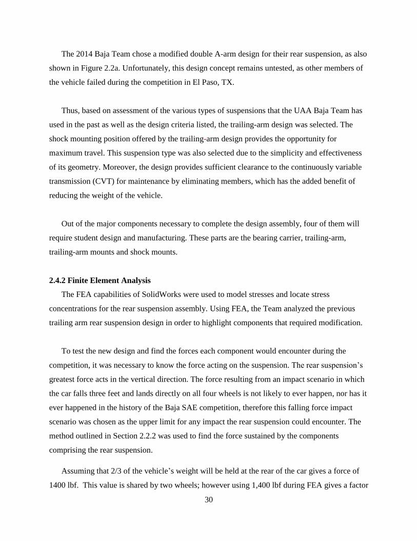
2.4.4 Bearing Carrier

The bearing carrier used in the 2013 trailing arm design was analyzed to determine if a new

bearing carrier needed to be designed. The bearing carrier was machined at UAA and the

material used was 6061-T6 stainless steel, which has a yield strength of 39,800 psi. Figure 2.4b

on the next page shows a modeled image of the 2013 rear bearing carrier.

Figure 2.4b. Rear bearing carrier from the

2013 Baja vehicle.

2.4.5 Mounting Devices

As a result of choosing a trailing arm suspension design, it was necessary to design new

mounts to support the chosen design. The mounts were created to accommodate the ½-inch rod

32

end’s mounting point from the trailing arm, as well as mount the suspension to the frame of the

car. The trailing-arm mount was designed using the 2014 mount as a model. The material chosen

was 4130 carbon steel, which comes in tubes as well as sheets. The part was modeled and

analyzed using the built in FEA within SolidWorks.

Also re-designed were the rear shock mounts. The part was designed to connect the top of

the shock to the frame. Although the same Fox Float shocks were used in this year’s design, the

previous design used 1020 carbon steel. This year, the rear shock mounts were redesigned using

4130 carbon steel sheet. As a result of this change, the car’s weight will be reduced, satisfying

one of the design goals for the rear suspension. The part was modeled and analyzed using FEA.

3.0 Results

The following sections outline the results and final designs of each sub-system. The overall

design of the vehicle improved performance and manufacturability of the frame, front suspension,

rear suspension, and control systems. The Team created a complete solid model of the entire car

and its components, which is ready for the fabrication process beginning in the spring of 2015, as

shown in Figure 3.0a below.

Figure 3.0a. Rendering of the final vehicle design.

33

3.1 Finalized Frame

The initial design of the frame needed only minor adjustments to improve it for the final

design. These minor changes were mostly implemented to accommodate the suspension systems.

The support member for the front shock, for example, had to be re-angled in order to absorb

more of the stress from the shock’s actuation. In addition, the rear end of the vehicle had to be

widened to allow the correct positioning of the rear suspension.

As the frame design progressed, members were also added for mounting elements of the

vehicle such as the brake and gas pedals, the shifter, the steering rack and the motor. The results

of the FEA studies done on the vehicle, covered in detail in the following section, however, did

not warrant changes to the design other than increased tubing size in select areas.

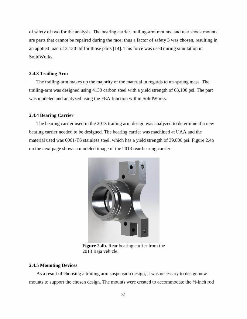
3.1.1 Frame Analysis Results

The results of the FEA studies done on the frame are summarized in Table 3.1a below.

Table 3.1a. Impacts for FEA analysis of the Baja vehicle with the force applied to the model for

simulation of the given scenario and the maximum stress that resulted.

Impact Scenario Applied Force Maximum Resulting Stress

Frontal Impact

1325 lbf

55,130 psi

Nose Dive Impact

3100 lbf

53,436 psi

Front Shock Impact

795 lbf 72,601 psi

Side/T-bone Impact

890 lbf 90,686 psi

Top Roll Impact

650 lbf 46,931 psi

Side Roll/Tipping Impact

650 lbf 74,776 psi

Skid Plate Vertical Impact

575 lbf 61,902 psi

Skid Plate Skidding Impact

890 lbf 35,256 psi

Rear Shock Impact

2130 lbf 61,944 psi

Rear Impact

880 lbf 77,214 psi

34

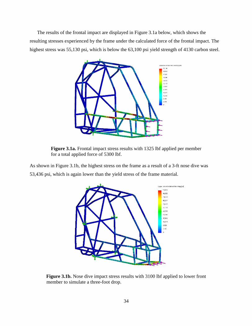
The results of the frontal impact are displayed in Figure 3.1a below, which shows the

resulting stresses experienced by the frame under the calculated force of the frontal impact. The

highest stress was 55,130 psi, which is below the 63,100 psi yield strength of 4130 carbon steel.

Figure 3.1a. Frontal impact stress results with 1325 lbf applied per member

for a total applied force of 5300 lbf.

As shown in Figure 3.1b, the highest stress on the frame as a result of a 3-ft nose dive was

53,436 psi, which is again lower than the yield stress of the frame material.

Figure 3.1b. Nose dive impact stress results with 3100 lbf applied to lower front

member to simulate a three-foot drop.

35

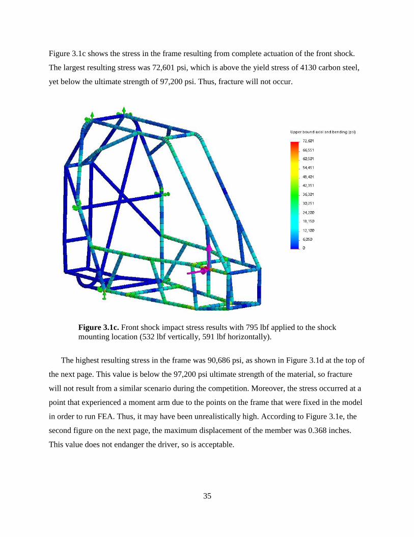
Figure 3.1c shows the stress in the frame resulting from complete actuation of the front shock.

The largest resulting stress was 72,601 psi, which is above the yield stress of 4130 carbon steel,

yet below the ultimate strength of 97,200 psi. Thus, fracture will not occur.

Figure 3.1c. Front shock impact stress results with 795 lbf applied to the shock

mounting location (532 lbf vertically, 591 lbf horizontally).

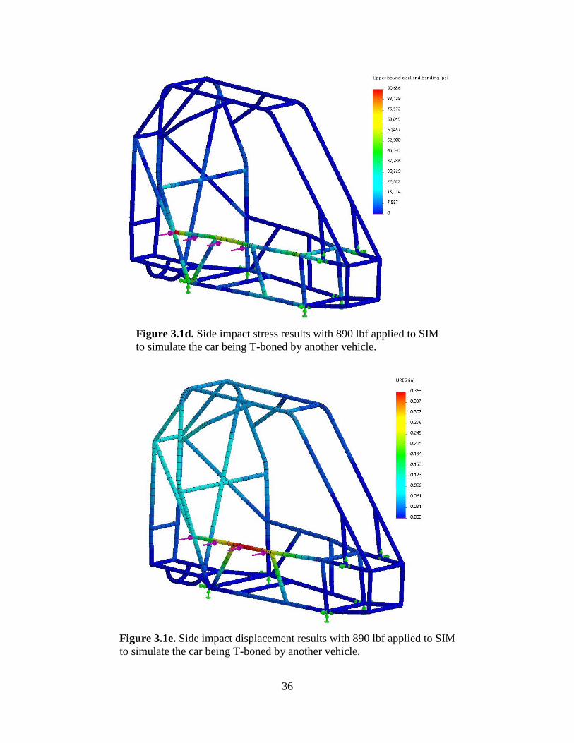
The highest resulting stress in the frame was 90,686 psi, as shown in Figure 3.1d at the top of

the next page. This value is below the 97,200 psi ultimate strength of the material, so fracture

will not result from a similar scenario during the competition. Moreover, the stress occurred at a

point that experienced a moment arm due to the points on the frame that were fixed in the model

in order to run FEA. Thus, it may have been unrealistically high. According to Figure 3.1e, the

second figure on the next page, the maximum displacement of the member was 0.368 inches.

This value does not endanger the driver, so is acceptable.

36

Figure 3.1d. Side impact stress results with 890 lbf applied to SIM

to simulate the car being T-boned by another vehicle.

Figure 3.1e. Side impact displacement results with 890 lbf applied to SIM

to simulate the car being T-boned by another vehicle.

37

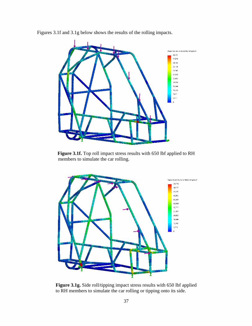
Figures 3.1f and 3.1g below shows the results of the rolling impacts.

Figure 3.1f. Top roll impact stress results with 650 lbf applied to RH

members to simulate the car rolling.

Figure 3.1g. Side roll/tipping impact stress results with 650 lbf applied

to RH members to simulate the car rolling or tipping onto its side.

38

The maximum force experienced during the top roll event was 46,931 psi, which is below the

yield of 4130 carbon steel. During the side roll or tipping event, the maximum stress was 74,776

psi, which is above yield, but below the ultimate strength of the material. Moreover, the stress

occurred at a fixed point in the model, meaning that the stress may be unduly high. The vehicle is

also unlikely to take such stress in the shown direction as if the car were to roll in this manner,

the full weight of the car would not be concentrated in the modeled direction. Thus, this stress

was deemed acceptable.

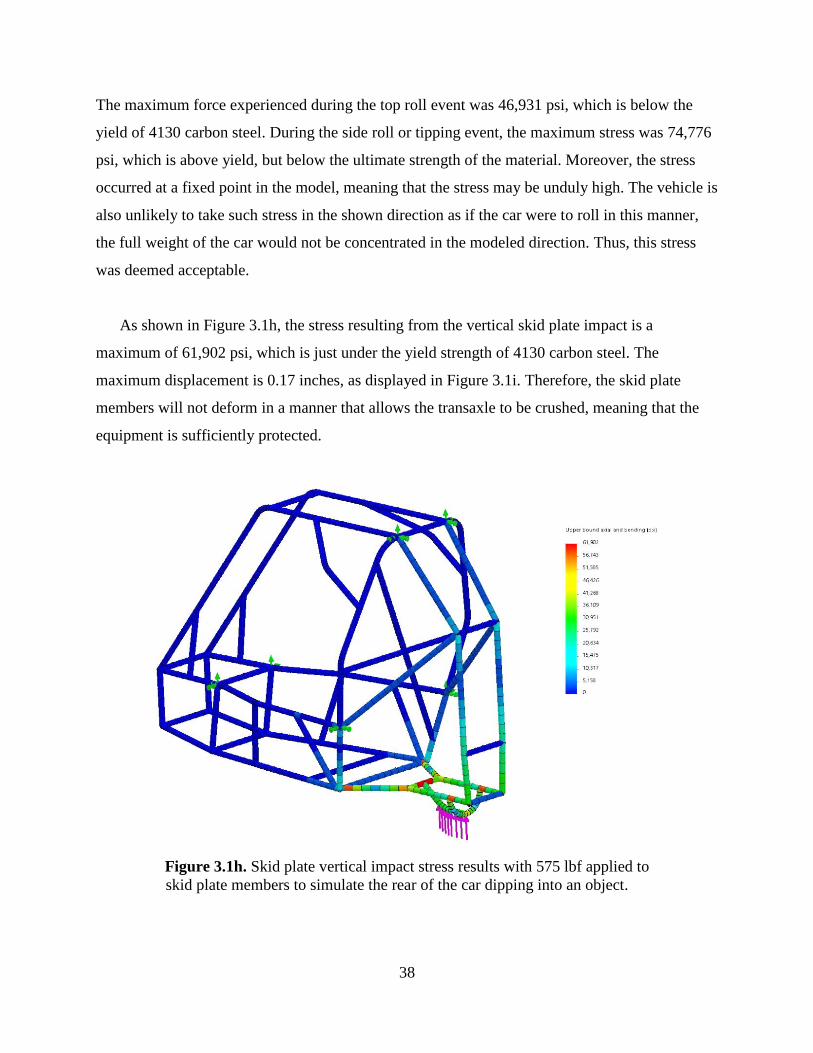
As shown in Figure 3.1h, the stress resulting from the vertical skid plate impact is a

maximum of 61,902 psi, which is just under the yield strength of 4130 carbon steel. The

maximum displacement is 0.17 inches, as displayed in Figure 3.1i. Therefore, the skid plate

members will not deform in a manner that allows the transaxle to be crushed, meaning that the

equipment is sufficiently protected.

Figure 3.1h. Skid plate vertical impact stress results with 575 lbf applied to

skid plate members to simulate the rear of the car dipping into an object.

39

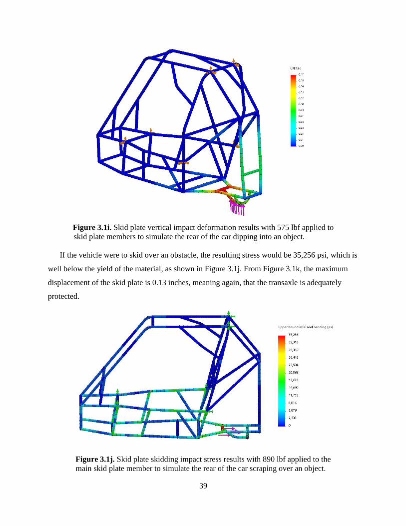
Figure 3.1i. Skid plate vertical impact deformation results with 575 lbf applied to

skid plate members to simulate the rear of the car dipping into an object.

If the vehicle were to skid over an obstacle, the resulting stress would be 35,256 psi, which is

well below the yield of the material, as shown in Figure 3.1j. From Figure 3.1k, the maximum

displacement of the skid plate is 0.13 inches, meaning again, that the transaxle is adequately

protected.

Figure 3.1j. Skid plate skidding impact stress results with 890 lbf applied to the

main skid plate member to simulate the rear of the car scraping over an object.

40

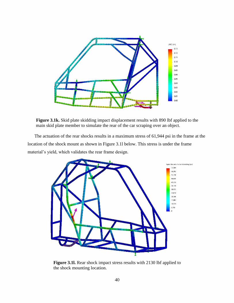
Figure 3.1k. Skid plate skidding impact displacement results with 890 lbf applied to the

main skid plate member to simulate the rear of the car scraping over an object.

The actuation of the rear shocks results in a maximum stress of 61,944 psi in the frame at the

location of the shock mount as shown in Figure 3.1l below. This stress is under the frame

material’s yield, which validates the rear frame design.

Figure 3.1l. Rear shock impact stress results with 2130 lbf applied to

the shock mounting location.

41

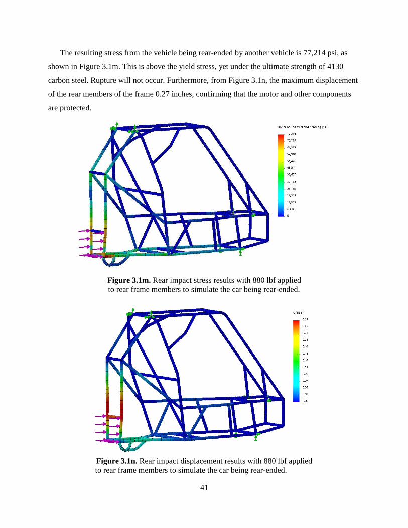
The resulting stress from the vehicle being rear-ended by another vehicle is 77,214 psi, as

shown in Figure 3.1m. This is above the yield stress, yet under the ultimate strength of 4130

carbon steel. Rupture will not occur. Furthermore, from Figure 3.1n, the maximum displacement

of the rear members of the frame 0.27 inches, confirming that the motor and other components

are protected.

Figure 3.1m. Rear impact stress results with 880 lbf applied

to rear frame members to simulate the car being rear-ended.

Figure 3.1n. Rear impact displacement results with 880 lbf applied

to rear frame members to simulate the car being rear-ended.

42

3.2 Front Suspension Study Results

After many front suspension design iterations, a balance of maneuverability, durability, and

overall weight was achieved. The vehicle’s handling was improved without sacrificing the

strength of key components. A thourough look at the kinematics of the vehicle resulted in a

suspension and steering system that moves through its full range of motion without affecting

fundamental relationships. A complete finite element analysis study was also performed to verify

the soundness of the materials chosen.

3.2.1 Front Suspension Geometry

The overall goal for this year’s front suspension and steering system design was to improve

the vehicles maneuverability. There are many elements in a vehicle’s front end geometry that

will affect how it performs off-road. The first of these elements is “bump steer”. Bump steer was

earlier defined as the tendency for a vehicle’s tires to turn in or out as the suspension moves

through its range of motion. This can adversely affect the driver’s ability to maintain control of

the vehicle when encountering rough terrain. It can also put an excessive amount of stress on the

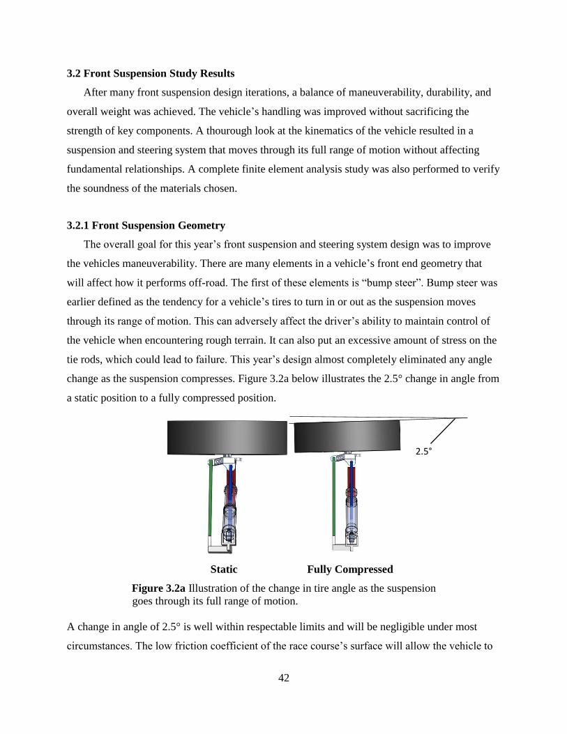
tie rods, which could lead to failure. This year’s design almost completely eliminated any angle

change as the suspension compresses. Figure 3.2a below illustrates the 2.5° change in angle from

a static position to a fully compressed position.

Static Fully Compressed

Figure 3.2a Illustration of the change in tire angle as the suspension

goes through its full range of motion.

A change in angle of 2.5° is well within respectable limits and will be negligible under most

circumstances. The low friction coefficient of the race course’s surface will allow the vehicle to

2.5°

43

track straight even if the full 2.5° change occurs.

Another important factor in a vehicle’s maneuverability is known as the Ackerman Steering

Ratio. As earlier discussed, this is the ratio of the radii of both front tires as the vehicle corners,

or makes turns. To keep the outside tire from slipping, the inside tire must follow a smaller

radius proportional to the track width of the vehicle. To achieve this result, the steering geometry

went through a complete redesign. The knuckles were rotated 180° and moved to opposite sides

of the vehicle. This allowed the axes intersecting the steering arms and kingpins to intersect at

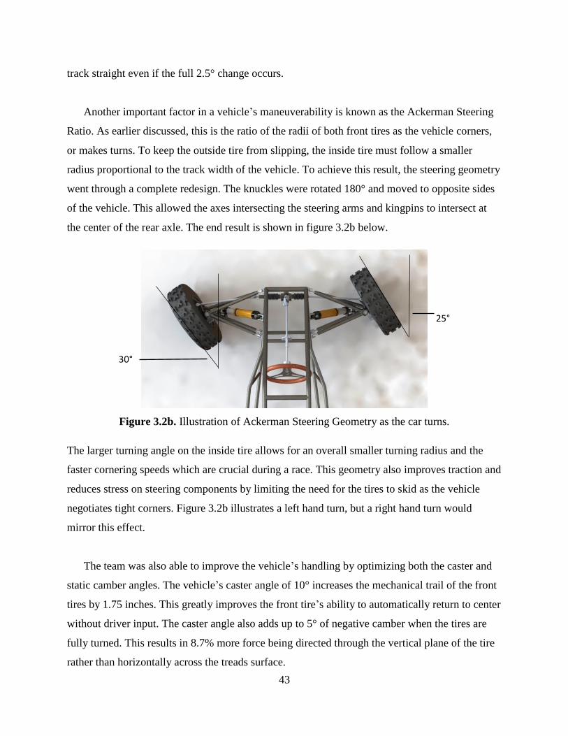
the center of the rear axle. The end result is shown in figure 3.2b below.

Figure 3.2b. Illustration of Ackerman Steering Geometry as the car turns.

The larger turning angle on the inside tire allows for an overall smaller turning radius and the

faster cornering speeds which are crucial during a race. This geometry also improves traction and

reduces stress on steering components by limiting the need for the tires to skid as the vehicle

negotiates tight corners. Figure 3.2b illustrates a left hand turn, but a right hand turn would

mirror this effect.

The team was also able to improve the vehicle’s handling by optimizing both the caster and

static camber angles. The vehicle’s caster angle of 10° increases the mechanical trail of the front

tires by 1.75 inches. This greatly improves the front tire’s ability to automatically return to center

without driver input. The caster angle also adds up to 5° of negative camber when the tires are

fully turned. This results in 8.7% more force being directed through the vertical plane of the tire

rather than horizontally across the treads surface.

30°

25°

44

A complete list of the front suspensions key parameters is shown in Table 3.2c.

Table 3.2a. Front suspension parameters.

Suspension Parameters

Suspension Type Dual unequal length A-arm

Shock Absorber Fox Float 3

Spring Rate exp(0.053x2+0.068x+5.323), at 70 psi

Vertical Wheel Travel 10 in

Track Width 53.90 in

Static Toe Angle 0 Degrees, Adjustable

Toe change over full travel (bump steer) +2.5 Degrees

Static Camber Angle -2 Degrees, Adjustable

Camber change over full travel +4.25 Degrees

Static Caster Angle 10 degrees, Non-Adjustable

Caster change over full travel 0 Degrees

Kingpin Inclination Angle 9.5 Degrees, Non adjustable

Mechanical Trail 2 in

Number of steering wheel turns lock to lock 3

Static Percent Ackerman 50%

Camber gain at lock 5 Degrees

Outside Turn Radius 7.7 ft

3.2.2 Finite Element Analysis

To verify that all the major components in the front suspension would endure the

predicted terrain they were analyzed under simulated loads using SolidWorks Simulation. Figure

3.2c on the following page shows 1060 lbf resulting from a 3 foot vertical drop being applied to

the lower A-arm. Because the lower A-arm is connected to the shock absorber, the entire vertical

force is transmitted through it. Therefore, the upper A-arm is not impacted by the force. The

force resulted in a maximum Von Mises stress of 62,350 psi, which is under the 63,100 psi yield

strength of 4130 alloy steel.

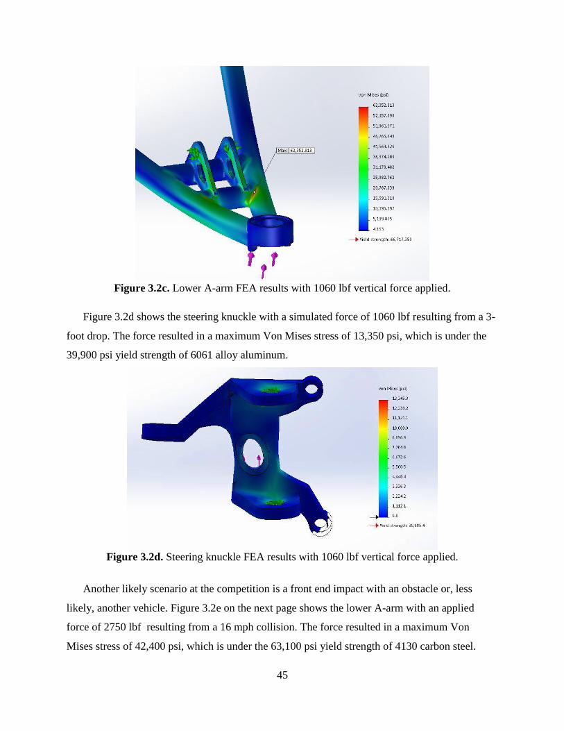
45

Figure 3.2c. Lower A-arm FEA results with 1060 lbf vertical force applied.

Figure 3.2d shows the steering knuckle with a simulated force of 1060 lbf resulting from a 3-

foot drop. The force resulted in a maximum Von Mises stress of 13,350 psi, which is under the

39,900 psi yield strength of 6061 alloy aluminum.

Figure 3.2d. Steering knuckle FEA results with 1060 lbf vertical force applied.

Another likely scenario at the competition is a front end impact with an obstacle or, less

likely, another vehicle. Figure 3.2e on the next page shows the lower A-arm with an applied

force of 2750 lbf resulting from a 16 mph collision. The force resulted in a maximum Von

Mises stress of 42,400 psi, which is under the 63,100 psi yield strength of 4130 carbon steel.

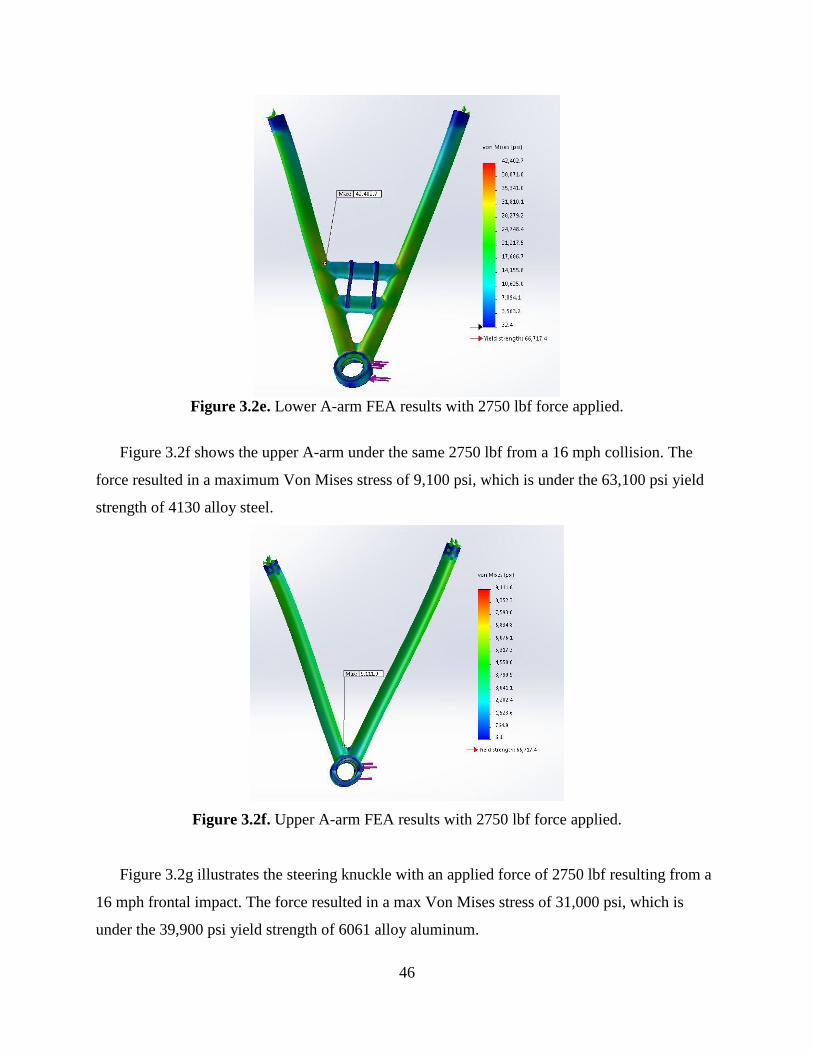
46

Figure 3.2e. Lower A-arm FEA results with 2750 lbf force applied.

Figure 3.2f shows the upper A-arm under the same 2750 lbf from a 16 mph collision. The

force resulted in a maximum Von Mises stress of 9,100 psi, which is under the 63,100 psi yield

strength of 4130 alloy steel.

Figure 3.2f. Upper A-arm FEA results with 2750 lbf force applied.

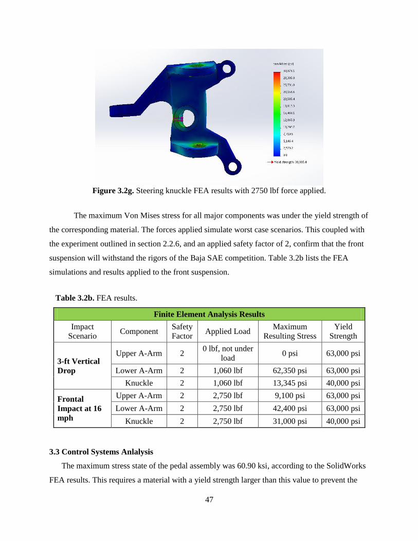
Figure 3.2g illustrates the steering knuckle with an applied force of 2750 lbf resulting from a

16 mph frontal impact. The force resulted in a max Von Mises stress of 31,000 psi, which is

under the 39,900 psi yield strength of 6061 alloy aluminum.

47

Figure 3.2g. Steering knuckle FEA results with 2750 lbf force applied.

The maximum Von Mises stress for all major components was under the yield strength of

the corresponding material. The forces applied simulate worst case scenarios. This coupled with

the experiment outlined in section 2.2.6, and an applied safety factor of 2, confirm that the front

suspension will withstand the rigors of the Baja SAE competition. Table 3.2b lists the FEA

simulations and results applied to the front suspension.

Table 3.2b. FEA results.

Finite Element Analysis Results

Impact

Scenario Component

Safety

Factor Applied Load

Maximum

Resulting Stress

Yield

Strength

3-ft Vertical

Drop

Upper A-Arm 2 0 lbf, not under

load 0 psi 63,000 psi

Lower A-Arm 2 1,060 lbf 62,350 psi 63,000 psi

Knuckle 2 1,060 lbf 13,345 psi 40,000 psi

Frontal

Impact at 16

mph

Upper A-Arm 2 2,750 lbf 9,100 psi 63,000 psi

Lower A-Arm 2 2,750 lbf 42,400 psi 63,000 psi

Knuckle 2 2,750 lbf 31,000 psi 40,000 psi

3.3 Control Systems Anlalysis

The maximum stress state of the pedal assembly was 60.90 ksi, according to the SolidWorks

FEA results. This requires a material with a yield strength larger than this value to prevent the

48

material from yielding. The yield strength of 1020 carbon steel is 50.99 ksi according to the

database of materials within the SolidWorks program, so this material would not be adequate for

most parts of the pedal assembly. 4130 Steel, annealed at 865°C has a yield strength of 66.72 ksi

according to the same database of materials, and it is a material that is available to the design

team. It was found that the lightest possible design could be achieved by using this material for

the fabricated parts of the assembly.

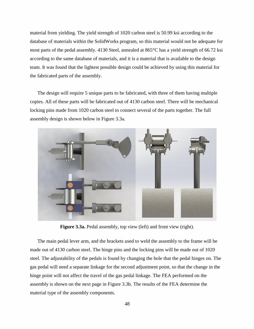
The design will require 5 unique parts to be fabricated, with three of them having multiple

copies. All of these parts will be fabricated out of 4130 carbon steel. There will be mechanical

locking pins made from 1020 carbon steel to connect several of the parts together. The full

assembly design is shown below in Figure 3.3a.

Figure 3.3a. Pedal assembly, top view (left) and front view (right).

The main pedal lever arm, and the brackets used to weld the assembly to the frame will be

made out of 4130 carbon steel. The hinge pins and the locking pins will be made out of 1020

steel. The adjustability of the pedals is found by changing the hole that the pedal hinges on. The

gas pedal will need a separate linkage for the second adjustment point, so that the change in the

hinge point will not affect the travel of the gas pedal linkage. The FEA performed on the

assembly is shown on the next page in Figure 3.3b. The results of the FEA determine the

material type of the assembly components.

49

Figure 3.3b. FEA results for the pedal assembly, side view (top) and front view (bottom).

The shifter will be mostly made out of 6061 aluminum. To accommodate for the stress

needed to withstand the large internal loads as a result of the relatively thin locking pin being

subjected to the design force of 40 lbf, the locking pin sections of the assembly will be made of

1020 carbon steel. Figure 3.3c shows the rendered shifter assembly.

Figure 3.3c. Side (left) and front (right) views of the shifter assembly.

The maximum stress shown by the FEA is 50.28 ksi. As can be seen in Figure 3.3d on the

following page that shows an isometric clipping of the stress in the shifter with the location of

the maximum stress being highlighted, this happens in the 1020 carbon steel segments of the

50

assembly, which is below the yield stress of 50.99 ksi for 1020 carbon steel. There is a node on

the aluminum locking bracket that exceeds the yield stress of 39.89 ksi. This indicates that there

will be some plastic deformation of the bracket at the interface between the locking bracket and

the 1020 carbon steel locking pin. However, the only way that this stress would be realistic is if

the locking/unlocking mechanism were fixed in place when the shifter handle is actuated, which

is a rare occurrence in race conditions. The natural motion to actuate the shifter is to remove the

pin first and then push the handle to shift gears, which makes the stress state of the shifter as seen

in Figure 3.3d below unlikely to happen.

Figure 3.3d. Isometric view of assembly FEA results with sections over the yield

strength of aluminum 6061 T6.

Figure 3.3 e on the next page shows general FEA results for the shifter.

51

Figure 3.3e. Side (left) and front (right) view of the FEA results for the shifter assembly.

3.4 Rear Suspension Iterations

After the FEA of the previous trailing-arm design, supporting material was added to the

trailing member to ensure this design would not break, although the addition countered the

Team’s goal to reduce the car’s weight. Thus, the trailing-arm was widened to accommodate the

new connection point and the bottom support shown in Figure 3.4a was extended closer to the

mounting points. This will increase the strength of the trailing-arm due to its larger triangular

geometry compared to the previous design. A midsection support was also added to prevent

deflection between the tubes.

Figure 3.4a. Rear suspension assembly model.

52

3.4.1 Bearing Carrier Results

The maximum stress that bearing carrier withstands was determine at 4,500 psi with an

applied load of 2120 lbf. Figure 3.4b shows the FEA study using SolidWorks. The bearing

carrier was tested and endured numerous types of terrain during the race in Bellingham, WA,

thus was deemed acceptable. A convergence study was also performed for the bearing carrier

within SolidWorks to ensure the study results were independent of the mesh size. Figure 3.4b

also shows a plot of the bearing carrier convergence study with degrees of freedom plotted

against the mesh size.

Figure 3.4b. Bearing Carrier with FEA stress study with 2120 lbf applied load to

simulated a three-foot drop and convergence study of degrees of freedom plotted against

mesh size.

3.4.2 Trailing-Arm Results

Figure 3.4c below shows the final model image of the trailing-arm after many iterations.

Figure 3.4c. Trailing-arm modeled and rendered with the use of SolidWorks.

0.000

0.050

0.100

0.150

0.200

0.250

0 500000 1000000 1500000 2000000

Me

sh s

ize

, in

D.O.F

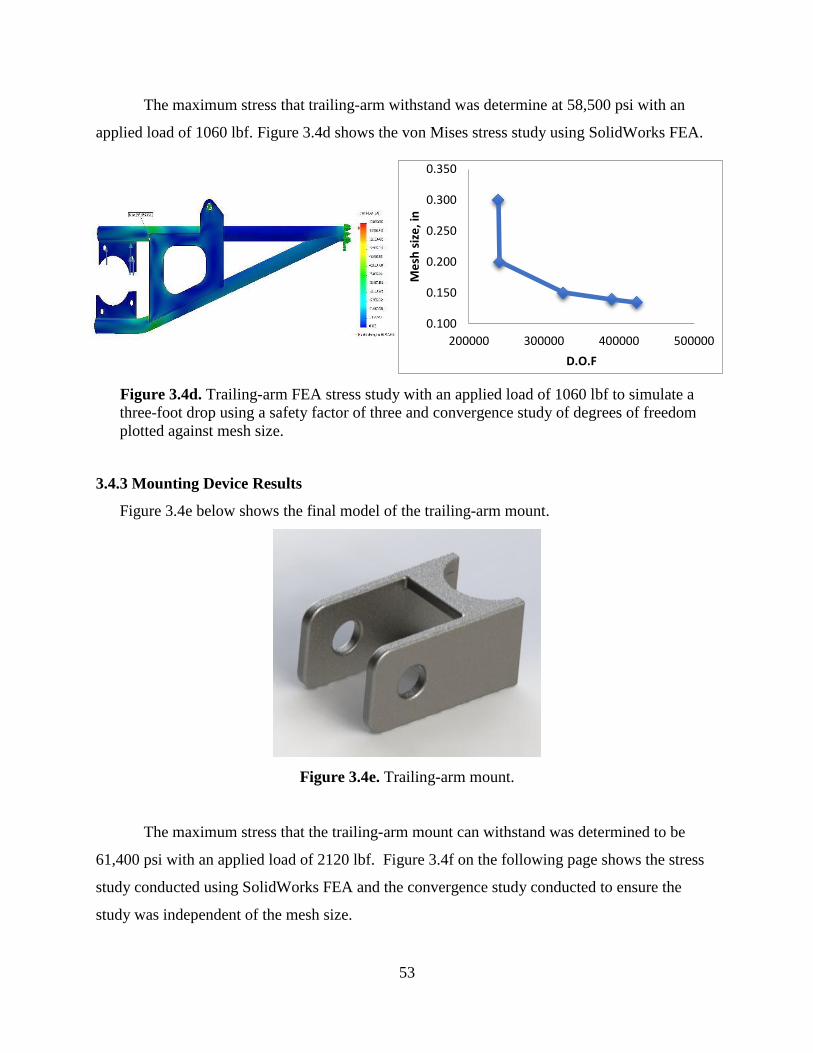
53

The maximum stress that trailing-arm withstand was determine at 58,500 psi with an

applied load of 1060 lbf. Figure 3.4d shows the von Mises stress study using SolidWorks FEA.

Figure 3.4d. Trailing-arm FEA stress study with an applied load of 1060 lbf to simulate a

three-foot drop using a safety factor of three and convergence study of degrees of freedom

plotted against mesh size.

3.4.3 Mounting Device Results

Figure 3.4e below shows the final model of the trailing-arm mount.

Figure 3.4e. Trailing-arm mount.

The maximum stress that the trailing-arm mount can withstand was determined to be

61,400 psi with an applied load of 2120 lbf. Figure 3.4f on the following page shows the stress

study conducted using SolidWorks FEA and the convergence study conducted to ensure the

study was independent of the mesh size.

0.100

0.150

0.200

0.250

0.300

0.350

200000 300000 400000 500000

Me

sh s

ize

, in

D.O.F

54

Figure 3.4f. Trailing-arm mount FEA stress study with an applied load of 2120 lbf

to simulate a three-foot drop using a safety factor of three and convergence study of

degrees of freedom plotted against mesh size.

Figure 3.4g below shows the final model image of the rear shock mount.

Figure 3.4g. Rear shock mount.

The maximum stress the rear shock mount withstands was determined to be 40,700 psi

with an applied load of 2120 lbf. Figure 3.4h shows the results of the stress study using

SolidWorks FEA and the convergence study conducted to ensure the study was independent of

the mesh size.

0.000

0.050

0.100

0.150

0.200

0.250

0 100000 200000 300000 400000 500000

Me

sh s

ize

, in

D.O.F

55

Figure 3.4h. Rear shock mount FEA stress study results with an applied load of 2120 lbf

from the simulation of a three-foot drop scenario and convergence study of degrees of

freedom plotted against mesh size.

4.0 Conclusion

The goal of the 2015 UAA Baja Team is to score within the top 20% at the international

Baja SAE competition in May 2015. To accomplish this goal, the group was divided into sub-

teams. Each sub-team followed the SAE Baja competition guidelines from the official rule book

and the scope of the senior design course. As a result, the 2015 Baja vehicle was engineered and

designed. The design of the vehicle improved performance and manufacturability of frame, front

suspension, rear suspension, and control systems from previous years. The Team created a

complete solid model of the entire car and its components, which is ready for the fabrication

process beginning in the spring of 2015.

5.0 References

[1] Brock, J. M. “Good Practices for Numerical Problem Solving.” Heat and Mass Transfer:

University of Alaska Anchorage. 2013. Lecture.

[2] SAE International. “2015 Collegiate Design Series: Baja SAE Rules.” 2015. Print.

[3] 2014 UAA Seawolf Motorsports Baja Team. “ME438 – Senior Design Report: Society of

Automotive Engineers Baja Vehicle.” Mechanical Design: University of Alaska Anchorage.

2013. Report.

[4] Hibbeler, R. C. “Engineering Mechanics: Statics & Dynamics.” 12th Edition. Upper Saddle

River, NJ: Pearson Education, Inc. 2010. Print.

[5] Millekin, W. F. “Race car vehicle dynamics.” 1st Edition. Warrendale, PA Society of

Automotive Engineers, Inc. 1995. Print.

0.000

0.050

0.100

0.150

0.200

0.250

0 100000 200000 300000 400000

Me

sh s

ize

, in

D.O.F

56

[6] “Understanding Ackerman Steering.” HotRodder. Web. October 2014. 2012.

[7] Bolles, B. “Caster and Camber Settings - Caster and Camber Tech.” Hot Rod Network. Web.

November 2014. 2008.

[8] “Friction and Coefficients of Friction.” The Engineering Toolbox. Web. November 12, 2014.

2014.

[9] Jaafer, Talib Ria, Mohmad Soib Selamat and Ramlan Kasiran. “Selection of Best

Formulation for Semi-Metallic Brake Friction Materials Development, Powder Metallurgy.”

Dr. Katsuyoshi Kondoh, ed. 2012. ISBN: 978-953-51-0071-3. InTech, DOI: 10.5772/33909.

[10] Brembo S.p.A. “Rear Master Cylinder PS12E.” Optimum Performance Products Inc. Web.

October 15, 2014. 2014.

[11] Bicknell Racing Products Inc. (2014). “Brake Balance Bar Set-Up.” Web. November 12,

2014. 2014.

[12] NASA. “Human Performance Capabilities.” Web. November 12, 2014. 2008.

[13] Corbin Rowe. Personal Interviews. September 2014 to November 2014.

[14] Kurowski, P. M. “Finite Element Analysis for Design Engineers.” Warrendale, PA: Society

of Automotive Engineers. 2004. Print.

6.0 Appendix A: Material Certification

from OnlineMetals.com

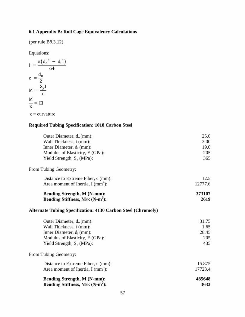
57

6.1 Appendix B: Roll Cage Equivalency Calculations

(per rule B8.3.12)

Equations:

(

)

κ = curvature

Required Tubing Specification: 1018 Carbon Steel

Outer Diameter, do (mm): 25.0

Wall Thickness, t (mm): 3.00

Inner Diameter, di (mm): 19.0

Modulus of Elasticity, E (GPa): 205

Yield Strength, Sy (MPa): 365

From Tubing Geometry:

Distance to Extreme Fiber, c (mm): 12.5

Area moment of Inertia, I (mm4): 12777.6

Bending Strength, M (N-mm): 373107

Bending Stiffness, M/κ (N-m2): 2619

Alternate Tubing Specification: 4130 Carbon Steel (Chromoly)

Outer Diameter, do (mm): 31.75

Wall Thickness, t (mm): 1.65

Inner Diameter, di (mm): 28.45

Modulus of Elasticity, E (GPa): 205

Yield Strength, Sy (MPa): 435

From Tubing Geometry:

Distance to Extreme Fiber, c (mm): 15.875

Area moment of Inertia, I (mm4): 17723.4

Bending Strength, M (N-mm): 485648

Bending Stiffness, M/κ (N-m2): 3633