university of alberta library release form · university of alberta library release form ......
TRANSCRIPT

University of Alberta
Library Release Form
Name of Author: Michelle Kenny
Title of Thesis: Optimization and Control Studies for Ammonia Production
Degree: Master of Science
Year this Degree Granted: 2001
Permission is hereby granted to the University of Alberta Library to reproduce single copies of
this thesis and to lend or sell such copies for private, scholarly or scientific research purposes
only.
The author reserves all other publication and other rights in association with the copyright in the
thesis, and except as herein before provided, neither the thesis nor any substantial portion thereof
may be printed or otherwise reproduced in any material form whatever without the author’s prior
written permission.
____________________ Michelle Kenny RR #2 Douglas, ON K0J 1S0

University of Alberta
Optimization and Control Studies for Ammonia Production
by
Michelle Kenny
A thesis submitted to the Faculty of Graduate Studies and Research in partial
fulfillment of the requirements for the degree of Master of Science
in
Process Control
Department of Chemical and Materials Engineering
Edmonton, Alberta
Fall 2001

University of Alberta
Faculty of Graduate Studies and Research
The undersigned certify that they have read, and recommend to the Faculty of Graduate Studies
and Research for acceptance, a thesis entitled Optimization and Control Studies for Ammonia
Production submitted by Michelle Kenny in partial fulfillment of the requirements for the degree
of Master of Science in Process Control.
_____________________ Fraser Forbes, Supervisor _____________________ C. Robert Koch _____________________ Biao Huang

ABSTRACT The need for nitrogen fertilizer is expected to significantly increase over the next twenty years[40].
Optimization and control may provide chemical manufacturers a means to support, in part, these
increased demands. This thesis explores automation prospects and technologies to exploit these
opportunities in the ammonia synthesis loop at Saskferco Products Inc. Existing research in this
field is not exhaustive and it is not apparent the most appropriate control technologies have been
implemented.
To accomplish these objectives, a dynamic first principles process model is developed
and fit to plant data. Using a rigorous nonlinear optimizer, the optimal operation of the unit is
evaluated. Enforcement of the optimal converter bed inlet temperatures is successfully
accomplished using linear PID and LQR controllers. Results clearly identify the opportunity for
improved ammonia conversion, with 70 % of these benefits achievable using a subset of the unit
optimizer and conventional controller methods.

CONTENTS 1. INTRODUCTION..................................................................................................................................1
1.1. Process Description .......................................................................................................................2 1.2. Process Considerations..................................................................................................................4 1.3. Process Automation.......................................................................................................................4 1.4. Thesis Scope..................................................................................................................................5 1.5. Thesis Conventions .......................................................................................................................6
2. AMMONIA PROCESS MODEL..........................................................................................................7 2.1. Characteristics of Conversion .......................................................................................................8 2.2. Constitutive Relationships...........................................................................................................11
2.2.1. Process Inputs and Conditioning ......................................................................................11 2.2.2. Chemical Reactions ..........................................................................................................12 2.2.3. Reaction Kinetics..............................................................................................................13 2.2.4. Heat of Reaction ...............................................................................................................14 2.2.5. Redlich-Kwong-Soave Equation of State .........................................................................14 2.2.6. Steam Calculations ...........................................................................................................15 2.2.7. Heat Transfer ....................................................................................................................16 2.2.8. Flow Through Valves and Process ...................................................................................17 2.2.9. Vessel Hold-Up ................................................................................................................19
2.3. Material & Energy Balances .......................................................................................................20 2.4. Model Implementation ................................................................................................................22 2.5. Model Validation.........................................................................................................................22 2.6. Discussion ...................................................................................................................................28
3. PARAMETER UPDATES USING HISTORICAL DATA ..............................................................31 3.1. Parameter Selection.....................................................................................................................31 3.2. Least Squares Regression Formulation .......................................................................................33
3.2.1. Sum of Squares .................................................................................................................34 3.2.2. Recursive Least Squares ...................................................................................................35
3.3. Results .........................................................................................................................................37 3.4. Discussion ...................................................................................................................................39
4. PROCESS OPERATION OPTIMIZATION.....................................................................................41 4.1. Optimization Problem Formulation.............................................................................................41 4.2. Sensitivity Analysis.....................................................................................................................42 4.3. Optimization Studies ...................................................................................................................45
4.3.1. Normal Operation .............................................................................................................45 4.3.2. Changing Process Conditions ...........................................................................................48 4.3.3. Degraded Catalyst.............................................................................................................52
4.4. Summary of Results ....................................................................................................................53 5. CONTROLLER SYNTHESIS ............................................................................................................55
5.1. State Space Analysis ...................................................................................................................56 5.2. BFW Level Implementation........................................................................................................58 5.3. Multi-Loop PID Control..............................................................................................................61
5.3.1. Multi-Loop Design ...........................................................................................................61 5.3.2. Multi-Loop Tuning ...........................................................................................................62 5.3.3. Multi-Loop Results...........................................................................................................64
5.4. Linear Multi-Variable Control ....................................................................................................75 5.4.1. MVC Design.....................................................................................................................75 5.4.2. MVC Tuning.....................................................................................................................76

5.4.3. MVC Results ....................................................................................................................77 5.5. Discussion ...................................................................................................................................85
6. SUMMARY AND CONCLUSIONS...................................................................................................88 6.1. Area of Study ..............................................................................................................................88 6.2. Results .........................................................................................................................................89 6.3. Conclusions .................................................................................................................................90 6.4. Recommendations .......................................................................................................................91
7. BIBLIOGRAPHY ................................................................................................................................92 A. PLANT DATA 96 B. GAS CONSTANTS AND EQUATIONS 116 C. MATLAB, SIMULINK AND MAPLE CODE 118 D. PROCESS MODEL 122
D.1 Calculations...............................................................................................................................122 D.2 Results .......................................................................................................................................124
E. PARAMETER UPDATE RESULTS 129 E.1 Dependent Variables .................................................................................................................129 E.2 Intermediate Variables ..............................................................................................................130 E.3 Results .......................................................................................................................................130
F. PROCESS OPTIMIZATION 133 G. CONTROLLER SYNTHESIS RESULTS 136
G.1 Controller Variables ..................................................................................................................136 G.2 Open Loop Responses ...............................................................................................................138 G.3 State Space Matrices .................................................................................................................141

LIST OF TABLES Table 2-1 Operating Conditions...............................................................................................................8 Table 2-2 Plant Input Variables .............................................................................................................11 Table 2-3 Fitted Parameters ...................................................................................................................23 Table 2-4 Catalyst Specifications ..........................................................................................................24 Table 3-1 Catalyst Manufacturer Parameter Calculations for R1B1 .....................................................32 Table 3-2 Model Parameters with Calculated Optimum Temperature ..................................................33 Table 3-3 Variable and Parameter Results for Parameter Update Problem ...........................................38 Table 4-1 R1B1 Impact of Temperature Deviation from Optimum ......................................................45 Table 4-2 Winter vs. Summer Optimal Operation .................................................................................52 Table 4-3 Ammonia Conversion: Optimal Performance Comparisons .................................................54 Table 5-1 PID Pairing ............................................................................................................................62 Table 5-2 PID Tuning ............................................................................................................................63 Table 5-3 Comparative Controller Behaviour with MV4 Saturated.......................................................86 Table 5-4 Comparative Controller Behaviour with MV1 Saturated.......................................................86 Table 5-5 Comparative Controller Characteristics ................................................................................87 Table A-1 Plant Data ..............................................................................................................................96 Table B-1 Gas Component Properties ..................................................................................................116 Table B-2 Gas Component Shomate Constants from 298 K to 1400K ................................................116 Table C-1 Process Simulation Files......................................................................................................118 Table C-2 RKS EOS Calculations........................................................................................................120 Table C-3 Catalyst Effectiveness Parameter Update Files ...................................................................120 Table C-4 Process Optimization Files ..................................................................................................121 Table C-5 State Space Matrices............................................................................................................121 Table C-6 Process Control Simulations................................................................................................121 Table E-1 Parameter Update Constraint Variables...............................................................................129 Table F-1 Dependent Variables per Equality Equations ......................................................................133 Table G-1 State Space Variables ..........................................................................................................136 Table G-2 Manipulated Variables.........................................................................................................136 Table G-3 Control Variables.................................................................................................................137 Table G-4 Disturbance Variables .........................................................................................................137 Table G-5 Local Value of A(x,u,w) Matrix ..........................................................................................141 Table G-6 Local Value of B(x,u,w) Matrix ..........................................................................................142 Table G-7 C Matrix ..............................................................................................................................143 Table G-8 Local Value of G(x,u,w) Matrix ..........................................................................................144 Table G-9 Local Value of A(x,u,w) Matrix – Reduced and Scaled......................................................145 Table G-10 Local Value of B(x,u,w) Matrix – Reduced and Scaled ......................................................146 Table G-11 C Matrix – Reduced and Scaled ..........................................................................................146

LIST OF FIGURES Figure 1-1 Ammonia Plant Overview ..................................................................................................1 Figure 1-2 Process Diagram .................................................................................................................3 Figure 2-1 Equilibrium Constant vs. Conversion Temperature............................................................9 Figure 2-2 Frequency Factor vs. Conversion Temperature ..................................................................9 Figure 2-3 Effect of Ammonia Concentration on Reaction Rate .......................................................10 Figure 2-4 Ammonia Conversion vs. Inlet Temperature to R1B1......................................................10 Figure 2-5 Knife Gate Valve Area .....................................................................................................17 Figure 2-6 Valve Output Characteristics ............................................................................................17 Figure 2-7 Gas-Gas Exchanger Fitted Data........................................................................................24 Figure 2-8 Gas-Gas Exchanger Results..............................................................................................25 Figure 2-9 Converter One Bed One Fitted Data.................................................................................25 Figure 2-10 Converter One Bed One Results .......................................................................................26 Figure 2-11 Overall Ammonia Conversion Fitted Data .......................................................................26 Figure 2-12 Overall Ammonia Conversion Results .............................................................................27 Figure 2-13 Waste Heat Boiler Steam Fitted Data ...............................................................................27 Figure 2-14 Waste Heat Boiler Steam Production Results...................................................................28 Figure 2-15 Synthesis Gas Feed ...........................................................................................................29 Figure 2-16 Synthesis Gas Hydrogen to Nitrogen Ratio in Feed Stream .............................................29 Figure 2-17 Synthesis Gas Inert Composition in Feed Stream.............................................................30 Figure 2-18 Synthesis Gas Ammonia Recycle in Feed Steam .............................................................30 Figure 3-1 Impact of Changing Model Parameters on Ammonia Reaction .......................................32 Figure 3-2 R1B1 Dynamic Parameter Update....................................................................................37 Figure 3-3 R1B1 Conversion Temperature Error ...............................................................................37 Figure 3-4 Overall Ammonia Production Error..................................................................................38 Figure 3-5 R1B1 Parameter Update vs. Inlet H/N Ratio ....................................................................40 Figure 4-1 R1B1 Conversion vs. Inlet Temperature, Varying Pressure .............................................43 Figure 4-2 R1B1 Conversion vs. Inlet Temperature, Varying H/N Ratio3.........................................44 Figure 4-3 R1B1 Conversion vs. Inlet Temperature, Varying yNH3 in Feed3......................................44 Figure 4-4 R1B1 Conversion vs. Inlet Temperature, Varying hx Parameter3 ....................................45 Figure 4-5 Optimal Temperature Profile, Normal Operation–Unit Optimization ..............................46 Figure 4-6 Optimal Ammonia Production, Normal Operation–Unit Optimization............................47 Figure 4-7 R2 Optimal Temperature Profile, Normal Operation–R2 Optimization...........................47 Figure 4-8 Optimal NH3 Production, Normal Operation-R2 Optimization........................................48 Figure 4-9 Summer vs. Winter Operation, H/N Ratio........................................................................49 Figure 4-10 Summer vs. Winter Operation, Synthesis Gas..................................................................49 Figure 4-11 Summer vs. Winter Operation, Process Inerts ..................................................................50 Figure 4-12 Summer vs. Winter Operation, Synthesis Gas Pressure ...................................................50 Figure 4-13 Summer vs. Winter Operation, Conversion ......................................................................51 Figure 4-14 Optimal Temperature Profile, Summer Operation............................................................51 Figure 4-15 Optimal Ammonia Production, Summer Operation..........................................................52 Figure 5-1 Waste Heat Boiler Level Open Loop Test ........................................................................59 Figure 5-2 WHB Level Closed Loop Step Test..................................................................................59 Figure 5-3 WHB Level Closed Loop Disturbance Test .....................................................................60 Figure 5-4 WHB Level Open to Closed Loop Test ............................................................................60 Figure 5-5 CV1 Step, PID, MV4 Saturated .........................................................................................65 Figure 5-6 CV2 Step, PID, MV4 Saturated .........................................................................................66 Figure 5-7 CV3 Step, PID, MV4 Saturated .........................................................................................67 Figure 5-8 CV1 Step, PID, MV1 Saturated .........................................................................................69 Figure 5-9 CV2 Step, PID, MV1 Saturated .........................................................................................70 Figure 5-10 CV3 Step, PID, MV1 Saturated .........................................................................................71 Figure 5-11 CV2 Step Down, Split Range Controller...........................................................................73 Figure 5-12 CV2 Step Up, Split Range Controller - CV Response.......................................................74

Figure 5-13 CV2 Step, Modified LQR, MV1 Saturated........................................................................78 Figure 5-14 CV1 Step, Final LQR, MV4 Saturated...............................................................................79 Figure 5-15 CV2 Step, Final LQR, MV4 Saturated...............................................................................80 Figure 5-16 CV3 Step, Final LQR, MV4 Saturated...............................................................................81 Figure 5-17 CV1 Step, Final LQR, MV1 Saturated...............................................................................82 Figure 5-18 CV2 Step, Final LQR, MV1 Saturated...............................................................................83 Figure 5-19 CV3 Step, Final LQR, MV1 Saturated...............................................................................84 Figure C-1 Simulink Block Diagram ................................................................................................119 Figure D-1 Converter One Preheat Exchanger Fitted Data ...............................................................124 Figure D-2 Converter One Preheat Exchanger Results .....................................................................124 Figure D-3 Converter One Bed Two Fitted Data ..............................................................................125 Figure D-4 Converter One Bed Two Results ....................................................................................125 Figure D-5 Converter Two Fitted Data .............................................................................................126 Figure D-6 Converter Two Results ...................................................................................................126 Figure D-7 Waste Heat Boiler I Fitted Data......................................................................................127 Figure D-8 Waste Heat Boiler I Results............................................................................................127 Figure D-9 Waste Heat Boiler II Fitted Data ....................................................................................128 Figure D-10 Waste Heat Boiler II Results ..........................................................................................128 Figure E-1 R1B2 Dynamic Parameter Update..................................................................................131 Figure E-2 R2 Dynamic Parameter Update ......................................................................................131 Figure E-3 R1B2 Conversion Temperature Error .............................................................................132 Figure E-4 R2 Conversion Temperature Error..................................................................................132 Figure G-1 CV1 Step, Open Loop .....................................................................................................138 Figure G-2 CV2 Step with MV1, Open Loop.....................................................................................139 Figure G-3 CV2 Step Up with MV4, Open Loop...............................................................................139 Figure G-4 CV2 Step Down with MV4, Open Loop..........................................................................140 Figure G-5 CV3 Step, Open Loop .....................................................................................................140

LIST OF SYMBOLS
ω Accentric factor
ƒ Fugacity, bar
υ Molar Volume, m3/mol
σ RKS Reduced Volume Shift
φ Fugacity Coefficient
τ PID Tuning Time Constant, minutes
λ Relative Gain Array
α RKS Attractive Parameter
σ2 Estimate Variance
ρ Density, kg/m3
Ωa RKS EOS coefficient, Ωa = 0.42748
Ωb RKS EOS coefficient, Ωb = 0.08664
∆Ek Activation Energy Term for Reverse Reaction (k_), J/mol N2
∆Ek_ Activation Energy for Reverse Reaction (k_), J/mol N2
∆LMIX Pipe Mixing Length for Bypass Valves, ∆LMIX = 1 m
∆PRXN Pressure Loss in Each Converter Bed, ∆PRXN = 0.1 MPa
SG
SG
VP
∆∆
Synthesis Gas Orifice Meter Pressure Differential Scaling Term
Φ Parameter Update Matrix
a RKS Intermediate Mix Calculation, J m3/mol2
aC,i RKS Pure Component Calculation at Critical Conditions, J.m3/mol2
A Shomate Constant
A RKS Intermediate Mix Calculation at Reduced Conditions (Appendix B)
A State Space Matrix for Process States (Chapter 5)
Ae Exchanger Heat Transfer Area, m2
Ai RKS Pure Component Calculation of Component i at Reduced Conditions
Av Pipe or Valve Flow Area, mm2
Ax Cross sectional area of vessel, m2
b RKS Intermediate Mix Calculation at Critical Conditions, m3/mol
bi RKS Pure Component Calculation at Critical Conditions, m3/mol

B Shomate Constant
B RKS Intermediate Mix Calculation at Reduced Conditions (Chapter B)
B State Space Matrix for Input Variables (Chapter 5)
Bi RKS Pure Component Calculation at Reduced Conditions
c RKS Intermediate Mix Calculation at Critical Conditions, m3/mol
ci RKS Pure Component Calculation at Critical Conditions, m3/mol
C Shomate Constant
C RKS Intermediate Mix Calculation At Reduced Conditions (Appendix B)
C State Space Matrix for Output Variables (Chapter 5)
Ci RKS Pure Component i Calculation At Reduced Conditions (Appendix B)
CP Heat Capacity, kJ/mol/K
D Shomate Constant
e Error
E Shomate Constant
E Energy, MJ
f Heat Transfer Correction Term (Chapter 2)
f Optimization Model Objective Function, kmol NH3/hr (Chapter 5)
fVOID Converter Catalyst Voidage Fraction
fx Fraction of Flow
F Shomate Constant
F Synthesis Gas Flow, kmol/s (Chapter 2)
F Calculated Process Variables (Chapter 3)
g Gravitational Constant, m/s2
gx Vessel Integral Time Correction Term
G Vessel Holdup of Synthesis Gas, kmol (Chapter 2)
G State Space Matrix for Disturbance Variables (Chapter 5)
Gw Vessel Holdup of Boiler Feed Water, kg
h Constraint Equality Equation for Optimization and Parameter Updates (Chapters
3 and 4)
h Enthalpy, kJ/mol (Chapter 2)
hR Residual Enthalpy, J/mol
ht Height of Level, m
hx Forward Reaction Parameter Estimate

H Enthalpy, kJ/kg
HV Hand Valve Position, % Output
HX Heat of Reaction, J/mol N2
J LQR Cost Function/Performance Index
k Reaction Frequency Factor, kmol NH3 /hr/m3 of catalyst/bar (Chapters 2 and 4)
k Attractive Parameter between Components (Appendix B)
ko Frequency Factor Constant, kmol NH3 /hr/m3 of catalyst/bar
K RKS EOS Intermediate Calculation (Appendix B)
K Gain Matrix (Chapter 5)
KP Overall Equilibrium Constant, bar-2 (Chapter 2)
L Level, % (Chapter 2)
L Estimator Gain for Kalman Filter (Chapter 5)
LV Level Valve Position, % Output
m Temkin constant, m = 0.46
M Mass Flow, kg/s or tonne/hr
MWT Gas Components’ Molar Masses, g/mol
n Moles in the Vessel, kmol
N LQR Weighting Matrix for Input and Output Variables
O Observability Matrix
p RKS EOS Attractive Parameter Calculation Coefficient
P Pressure, Paa, MPaa or reduced (Chapter 2)
P Controllability Matrix (Chapter 5)
Q Heat Transfer Across the Exchanger, MW (Chapter 2)
Q LQR Weighting Matrix for Output Variables (Chapter 5)
r Valve Bore Radius, mm
rxn_coeff Vector of Stoichiometric Coefficients,
= [ +1 –0.5 –1.5 0 0 0]
= [ NH3 N2 H2 He Ar CH4]
R Ideal Gas Constant, R = 8.314 J/mol/K (Chapter 2)
R LQR Weighting Matrix for Input Variables (Chapter 5)
RXN Rate of the Overall Reaction, kmol NH3/h
S Riccati Matrix
t Time, seconds or minutes
T Temperature, K, mK, oC, reduced or differential
u Manipulated variable or parameter
U Exchanger Heat Transfer Coefficient, W/m2/K
v Linear Velocity, m/s
V Flow of Synthesis Gas Entering Unit at STP, 1000 standard m3/h
Vol Volume, m3
w Disturbance Variables
W Weighting Matrix: Inverse of Covariance Matrix
x State Space Variables
X Half the Width of the Valve Position At Height Y, mm
y Vector of Mole Fractions, mol/mol (Chapter 2 and Appendix B)
= [ yNH3 yN2 yH2 yHe yAR yCH4]
= [ y1 y2 y3 y4 y5 y6]
y Optimization Variables (Chapter 4)
y Measured Process or Output Variables (Chapter 5)
Y Height of the Valve Opening, mm
Z Compressibility Factor

LIST OF ACRONYMS BFW Boiler Feed Water
CBD Continuous Blowdown
CPUTime Processing Time based on AMD Athlon 500 MHz processor with 512 MB RAM,
minutes
CV Control Variable
Dev’n Deviation
DV Disturbance Variable
EOS Equation of State
H:N or H/N Reactant Hydrogen to Nitrogen Mole Ratio
HOLDUP Vessel Holdup Volume
ODE Ordinary Differential Equation
LSR Least Squares Regression
LQR Linear Quadratic Regulator
LQGR Linear Quadratic Gaussian Regulator
MIMO Multiple Input Multiple Output
MP Medium Pressure
MPC Multi-Variable Predictive Control
MV Manipulated Variable
MVC Multi-Variable Controller
PID Proportional Integral Derivative Control
R1 Ammonia Converter One
R1B1 Ammonia Converter One, Bed One
R1B2 Ammonia Converter One, Bed Two
R1PH Ammonia Converter One, Preheat Exchanger
R2 Ammonia Converter Two
RLS Recursive Least Squares
RKS Redlich-Kwong-Soave
SISO Single Input Single Output
SG Synthesis Gas
WHB I Waste Heat Boiler One
WHB II Waste Heat Boiler Two
WHB Waste Heat Boiler
LIST OF SUBSCRIPTS + Forward Reaction
_ Reverse Reaction Properties
(a) Refers to the component absorbed onto the catalyst
298.15° Reference Temperature
ACT Actual, Measured Value
AR Argon
ATM Atmospheric Pressure
AVG Average
BY Valve Bypass Stream
BY1 Bypass Stream One
BY2 Bypass Stream Two
BFW Boiler Feed Water
BFW-B Waste Heat Boiler II Bottom Area Boiler Feed Water
BFW-M Waste Heat Boiler II Middle Area Boiler Feed Water
BFW-T Waste Heat Boiler II Top Area Boiler Feed Water
C Property Critical Constants (Chapter 2, Appendix B)
C Controller Properties (Chapter 5)
CALC Model Calculation
CBD Continuous Blowdown
CH4 Methane
CORR Corrected for temperature, pressure and/or composition
D Derivative
ERR Error
f,298 Formation at 298 K
G/G Gas-Gas Exchanger
H2 Hydrogen
HE Helium
Holdup Vessel Holdup Capacity
i Component i [NH3, N2, H2, He, Ar CH4] or counter
I Integral
IG Ideal Gas Property
IN Inlet Stream

j Component j [NH3, N2, H2, He, Ar CH4] or counter
k_ Reverse Reaction, NH3 Decomposition, Property
m Mean
MIX Mix Property (length)
mK milli-Kelvin (units)
n Process Sample Set, Time Period Reference
N2 Nitrogen
NEW New Process Characteristics
NH3 Ammonia
OLD Previous Process Conditions
OUT Outlet Stream
OP Valve Output/Position
P Processes Properties
PLANT Measured process variable
R Reduced Property
R1 Ammonia Converter One
R1B1 Ammonia Converter One, Bed One
R1B2 Ammonia Converter One, Bed Two
R1PH Converter One Preheat
R2 Ammonia Converter Two
REF Reference, Design Value
RES Residual Property
RNG Range of Values
RXN Ammonia Reaction Property
SG Synthesis Gas
SHELL Shell Side of Heat Exchanger
SHELL-B WHB II Shell Bottom Heat Transfer Area of Vessel
SHELL-M WHB II Shell Middle Mix Area of Vessel
SHELL-T WHB II Shell Top Mix Area of Vessel
STD Standard Deviation
STEAM Steam from Waste Heat Boilers
STP Standard Temperature and Pressure
TUBE Tube Side of Heat Exchanger
VALVE Valve Property

VESSEL Reference to Exchanger or Converter Vessel
WHBI Waste Heat Boiler One
WHBII Waste Heat Boiler Two

LIST OF SUPERSCRIPTS o Pure Components
* Optimal Solution
^ Estimated Variable
· Rate Equation, units/time
1
CHAPTER 1
INTRODUCTION
Farmers around the world currently use 87 million tonnes of nitrogen fertilizer per year[31], which
is produced from approximately 400 ammonia plants[22]. Extrapolating farming trends to the year
2020, the mean forecast for global nitrogen fertilization is an increase of 60 % from present
amounts[40].
As agricultural requirements continue to expand, demand to increase nitrogen fertilizer
supply will inevitably push producers to consider growth opportunities within existing plant
facilities. Advanced process control will play a role in meeting this demand. While opportunities
exist throughout the ammonia process, this thesis focuses on control of the ammonia synthesis
unit.
This thesis explores the control and optimization of the ammonia synthesis loop at
Saskferco Products Inc. By maximizing reactor conversions, increased production can potentially
be achieved. Improved conversion directly impacts synthesis gas recycle and energy consumption
per tonne of product.
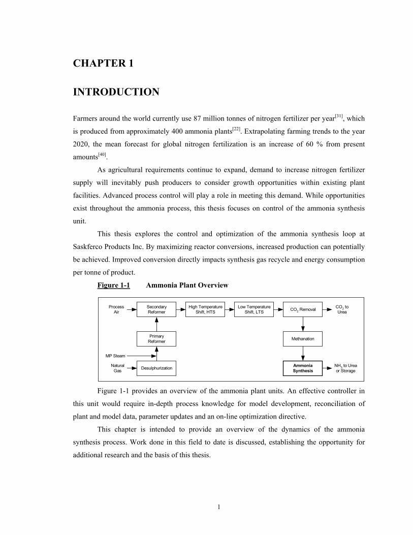
Figure 1-1 Ammonia Plant Overview
DesulphurizationNaturalGas
PrimaryReformer
SecondaryReformer
High TemperatureShift, HTS
Low TemperatureShift, LTS CO2 Removal
Methanation
AmmoniaSynthesis
ProcessAir
MP Steam
CO2 toUrea
NH3 to Ureaor Storage
Figure 1-1 provides an overview of the ammonia plant units. An effective controller in
this unit would require in-depth process knowledge for model development, reconciliation of
plant and model data, parameter updates and an on-line optimization directive.
This chapter is intended to provide an overview of the dynamics of the ammonia
synthesis process. Work done in this field to date is discussed, establishing the opportunity for
additional research and the basis of this thesis.
2
1.1. Process Description
The synthesis of ammonia from hydrogen and nitrogen over an iron catalyst, commonly known as
the Haber process, is an industrially important reaction[25]. The Haber process has been well
characterized. This section reviews the basic principles of the ammonia synthesis as it applies to
industry.
Ammonia synthesis is exothermic and after the reaction has been established, it is self-
sustaining. The reaction mechanism is governed by the reaction in Equation 1.1.
322 NH H23 N
21
⇔+ (1.1)
The process studied in this thesis is based on the operation of Saskferco Products Inc. in
Belle Plaine, Saskatchewan, Canada1. Saskferco is one of the largest single train nitrogen
fertilizer plants in the world, producing approximately 1,850 tonnes per day of anhydrous
ammonia and 2,850 tonnes per day of granular urea. Figure 1-2 shows the process flow diagram
of the ammonia synthesis unit studied.
High-pressure synthesis gas is fed to the unit from the synthesis gas compressor.
Conversion occurs over three beds of iron based catalyst. Reactant gas is cooled between beds to
improve conversion. Heat is removed from the unit through the generation of high-pressure steam
in the waste heat boilers. The outlet gas, containing approximately 18 % ammonia, exits the unit
where the ammonia product is separated from the unreacted components. The unreacted synthesis
gas is then recycled back to the converters. Detailed operation of the ammonia converters
including, operating conditions, process constraints, instrumentation, existing applications and
proposed process changes is reviewed in Chapter 2.
1 References to data and operation of this facility are bound by the Saskferco – University of Alberta secrecy
agreement[17].

Figure 1-2 Process Diagram
SYNTHESIS GAS COMPRESSOR
TI
PI
AINH3,CH4,N2, H2,AR, He
TIHIC
TI
HIC
TI(6)
TI AI
NH3 PRODUCT
TI
SYNTHESISGASRECYCLE
FI
SYNTHESISGAS
TI(6)
TI
HIC
PIHIC
FI FY
LIC
BOILERFEED
WATER
FI
STEAM
CONT.BLOWDOWN
TI
TI
TI(2)
TI
TI
NH3,CH4,N2, H2,AR, He
GAS-GASEXCHANGER
CONVERTERI
WASTEHEAT
BOILER I
WASTEHEAT
BOILER II
CONVERTERII
INERTS
CONT.BLOWDOWN
FI
LEGENDAI ANALYZER INDICATORFI FLOW INDICATORFY FLOW CALCULATIONHIC HAND VALVE INDICATION CONTROLLERLIC LEVEL INDICATION CONTROLLERPI PRESSURE INDICATORTI TEMPERATURE INDICATOR
3
4
1.2. Process Considerations
Ammonia synthesis poses several engineering challenges including nonideal and nonlinear
behaviour, as well as a moving optimal operation of the unit
The high pressure of commercial operations, dictated by the reaction kinetics provides an
interesting case study for thermodynamic nonidealities. In this case, the Redlich-Kwong-Soave
equation of state (RKS EOS) is used to account for residual enthalpies, gas compressibility and to
calculate the fugacity of the gas reactants.
Although ammonia conversion is favoured by low temperatures, the reaction kinetics of
this exothermic reaction are not. This introduces strong process nonlinearities with respect to the
overall ammonia conversion and the operating temperature. If the operating temperature is
reduced below the optimum, the production of ammonia can drop off rapidly and the potential
exists for the reaction to lose its self sustainability. Consequently, reaction temperatures are
operated at a safe open loop differential above the optimum. While this increases the reaction
rate, it has a negative impact on the equilibrium and subsequently the amount of ammonia
produced. Implementation of a linear controller to the ammonia process is simplified by selection
of the control variables with the most linear response to the manipulated variables.
Changing feed composition and pressure contribute to a variable optimum reaction
temperature. The inerts in the feed stream (methane, argon and helium) lower the reactant partial
pressures and the conversion potential. Ammonia in the recycle gas also has a negative impact on
the net ammonia production. The ratio of reactants, referred to as the hydrogen to nitrogen (H/N)
ratio, also shifts the optimum temperature.
1.3. Process Automation
Due to the nonlinear and nonideal nature of the process, outlined above, research and practical
application of closed loop control on the ammonia synthesis loop has been limited. Recognizing
nitrogen fertilizer as an important aspect of farming and world food production, with growing
demand[40], opportunities to improve the efficiency and throughput of existing plant
manufacturers should be evaluated.
Saskferco is a state of the art ammonia/urea plant commissioned in 1992. Similar to other
ammonia plants, Saskferco currently uses ratio control to manipulate the H/N ratio into the
converter. PID control is also available for the inlet temperature of the third reactor bed.
However, due to problems with the control valve, and without a mechanism to determine the
optimal setpoint, this controller is operated only in manual mode.

5
Industrial examples of advanced control that encompass all of the reactor beds are less
common. Multivariable control implementations on multibed ammonia converters with direct
cooling (quench converters) are documented by several control vendors[19],[22],[28]. These
implementations have recorded benefits between 1 to 2 % of total ammonia production. However,
implementation details and the control options that were explored have not been publicized.
Information not explicitly addressed in these implementations includes update of parameter
estimates, to account for model mismatch, and on-line optimization of the nonlinear process. This
thesis addresses these issues for multibed ammonia converters with indirect cooling.
Similar research in this area, which has been the subject of several publications[11],[13],[25],
includes the optimal design of the ammonia converter beds.
1.4. Thesis Scope
This thesis attempts to identify the optimization and control opportunities of an existing ammonia
synthesis process and the means to achieve these benefits. To date, research into the control
options and the supporting tools necessary to properly implement this control has been limited.
While multi-variable control (MVC) applications have been successfully put into service, it is not
clear that claimed benefits could not have been realized with less complicated control strategies.
Additionally, on-line tools needed to realize these benefits have been either overlooked or
oversimplified. This thesis provides an evaluation of the optimization problem, complete with
parameter updates. Control options such as a simple PID controller and a slightly more
complicated MVC are implemented and compared.
Chapter 2 delves into the kinetic and thermodynamic properties of ammonia synthesis.
Thermodynamic properties are based on the RKS EOS with the Temkin-Pyshev equation used to
describe the synthesis process. Reconciliation of model results with plant data is explored.
Parameter updates, using historical plant data, are explored in Chapter 3. Variations of
the least squares approach are evaluated. Using three parameters, four measured variables are
predicted. The parameter update results are employed in the optimization model.
Process optimization is discussed in detail in Chapter 4. Potential benefits for various
modes of operation are considered. Both process constraints and sensitivities are addressed.
Opportunities and potential benefits using a simplified optimization routine are compared to an
overall unit optimizer.
Having established the criteria required to achieve effective control, controllability of the
system is considered in Chapter 5. Control, manipulated and disturbance variables are
determined. The relative gain array (RGA) is used to determine appropriate coupling of these
6
variables for PID control. Multi-loop PID and a MVC are designed and tested. Performance in
both cases is compared.
The thesis provides recommendations to Saskferco to improve the performance of the
ammonia synthesis loop through the implementation of parameter updates, optimization and
control.
1.5. Thesis Conventions
A consistent set of symbols is used throughout each chapter of the thesis. These symbols are
defined at the beginning of the document.
Other standard conventions used in the body of the thesis are described. Plant refers to
the process at Saskferco Products Inc. The term model refers to the Matlab and Simulink
simulation, developed based on first principles and fit to plant data. Process can be used to
describe the operation of either the plant or the simulation. Sample sets and shift averages refer
to plant data collected from the process, using 12-hour shift averages.
The process model contains states, inputs and parameters. A state variable arises
naturally in the accumulation term of the dynamic material or energy balance[4]. It is often a
measured value, used to characterize the system. Inputs are the inlet conditions of the process,
required for operation. This includes variables that are manipulated to achieve desired
performance. Parameters are defined as the constant values or coefficients included in the model
calculations. These parameters include chemical and physical values.
Variables used for parameter updates and process optimization are broken down into
dependent (tear) and independent (manipulated) variables. Dependent variables are the direct
result of operation at a specified set of values for the independent variables. Manipulated
variables are independently adjusted to achieve the model objective function.
Controller variables include control variables, manipulated variables and disturbance
variables. Control variables are the controller outputs used to regulate the process. Manipulated
variables are the controller inputs, used to achieve the desired control variable. In this thesis, the
manipulated variables are the control valve positions. Disturbance variables are independent
inputs into the process that cannot be manipulated.
The dynamic process model makes several assumptions, such as radial flow through the
converter beds and uniform pressure in each vessel. Heat loss to the environment is assumed
negligible. Heat transfer characteristics of the vessels and reactor pellets are not modelled.
7
CHAPTER 2
AMMONIA PROCESS MODEL
The process considered in this thesis is based on the operation and design of the ammonia
synthesis loop at Saskferco Products Inc in Belle Plaine, Saskatchewan. In the following section,
the process is described at normal plant operating conditions.
The ammonia synthesis unit is comprised of a gas-gas heat exchanger, two converters
(three reaction beds in total) and two waste heat boilers, as shown in Figure 1-2.
The synthesis gas feed is a mix of fresh make-up gas and unconverted recycle gas. Inert
process gases in the synthesis gas are primarily a function of the upstream units. Equipment
limitations at high feed rates and summer temperatures have a negative impact on the ability to
remove inerts from the recycle gas stream. The main detrimental effect of inerts in the synthesis
gas is to reduce the effective partial pressure of the reactants and thus the conversion rate[25].
Similar to inert recycle, the amount of recycled ammonia is related to feed throughput and the
ambient temperature. In addition to reducing the partial pressure of the reactants, recycled
ammonia reduces the net ammonia production potential. The H/N feed mole ratio is controlled to
about 3.1 moles of hydrogen per mole of nitrogen using a PID ratio controller. H/N control is not
achievable in the summer months due to reduced ambient air density and the saturated output of
the air compressor. Production gas leaving the unit is sent to the process chillers for the
separation of ammonia, inerts and recycle gas. Table 2-1 summarizes the operating conditions of
the plant.
Four bypass valves exist on the unit. The first valve, around the shell of the gas–gas
exchanger is kept closed except for start-up conditions. A bypass valve around the preheat
exchanger (R1PH) tubes in the first converter (R1) acts as a cold shot to the first reaction bed
inlet temperature. This valve can be used to manipulate both the bed one (R1B1) and bed two
(R1B2) inlet temperatures and typically remains closed. The valve around the tube side of the
first waste heat boiler (WHB I) is used to manipulate the second converter (R2) inlet temperature.
The normal operation of this valve is open loop with a valve position of about ninety percent. The
boiler feed water (BFW) inlet flow to the second waste heat boiler (WHB II) can be split between
the top and the bottom of the shell. Increasing flow to the top of the exchanger reduces the overall
heat transfer in this vessel.

8
Table 2-1 Operating Conditions
Operating Parameters Typical Operating Conditions
VIN,SG 799 k-sm3/hr
TIN,SG 27 oC
PIN,SG 18.6 MPag
yIN = [yNH3 yH2 yN2 yHe yAR yCH4] [0.02 0.20 0.63 0.01 0.03 0.11]
TG/G,SHELL 282 oC
TR1PH,TUBE 377 oC
TR1PH,SHELL 407 oC
TR1B1 511 oC
yR1B1 [0.12 0.17 0.55 0.01 0.03 0.12]
TR1B2 464 oC
yR1B2 [0.17 0.16 0.50 0.01 0.03 0.13]
TWHBI,TUBE 345 oC
TWHBI,BY 398 oC
TR2 442 oC
yR2 [0.21 0.14 0.47 0.01 0.03 0.14]
TWHBII,TUBE 320 oC
TG/G,TUBE 54 oC
In designing a controller using the WHB II BFW valve, it should be noted that large
output changes introduce swings into the plant steam header pressure. The consequence of this is
a possible loss of control in the BFW level in WHB II and subsequent shutdown of the entire
ammonia plant. Due to the small hold-up of BFW in this vessel, a plant trip can occur in less than
one minute.
2.1. Characteristics of Conversion
The conversion of ammonia from hydrogen and nitrogen has nonlinear process properties largely
due to competing equilibrium and kinetic forces.
The equilibrium favours a low temperature and high pressure. Figure 2-1 shows the
decaying exponential relationship between the equilibrium constant for ammonia conversion and
the conversion temperature at a pressure of 19 MPa.

9
Figure 2-1 Equilibrium Constant vs. Conversion Temperature
1.E-10
1.E-05
1.E+00
1.E+05
1.E+10
0 200 400 600 800 1000Conversion Temperature, oC
Equi
libri
um C
onst
ant,
bar-
2
The kinetics are accelerated by increased operating temperatures[1]. As shown in Figure
2-2 both the forward and reverse reactions occur at a higher rate as the temperature is increased.
Figure 2-2 Frequency Factor vs. Conversion Temperature
1.E-20
1.E-10
1.E+00
1.E+10
0 200 400 600 800 1000Conversion Temperature, oC
Equi
libri
um R
eact
ion
Rat
e Fr
eque
ncy
Fact
or
Reverse Reactionkmol NH3/hr/m3 catalyst/bar^1.46
Forward Reactionkmol NH3/hr/m3 catalyst/bar^-0.54
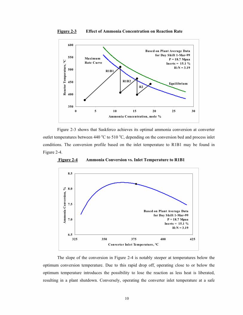
Figure 2-3 illustrates the effect of the ammonia concentration on the equilibrium and
optimum temperature curves, using actual plant data.
10
Figure 2-3 Effect of Ammonia Concentration on Reaction Rate
350
400
450
500
550
600
0 5 10 15 20 25 30
Ammonia Concentration, mole %
Rea
ctor
Tem
pera
ture
, °C
Equil ibrium
Maximum Rate Curve
R1B1
R1B2
R2
Based on Plant Average Data for Day Shift 1-Mar-99
P = 18.7 MpaaInerts = 15.1 %
H:N = 3.19
Figure 2-3 shows that Saskferco achieves its optimal ammonia conversion at converter
outlet temperatures between 440 oC to 510 oC, depending on the conversion bed and process inlet
conditions. The conversion profile based on the inlet temperature to R1B1 may be found in
Figure 2-4.
Figure 2-4 Ammonia Conversion vs. Inlet Temperature to R1B1
6.5
7.0
7.5
8.0
8.5
325 350 375 400 425Converter Inlet Temperature, °C
Am
mon
ia C
onve
rsio
n, %
Based on Plant Average Data for Day Shift 1-Mar-99
P = 18.7 MpaaInerts = 15.1 %
H:N = 3.19
The slope of the conversion in Figure 2-4 is notably steeper at temperatures below the
optimum conversion temperature. Due to this rapid drop off, operating close to or below the
optimum temperature introduces the possibility to lose the reaction as less heat is liberated,
resulting in a plant shutdown. Conversely, operating the converter inlet temperature at a safe
11
margin above the optimum slightly reduces ammonia conversion and provides some latitude for
plant disturbances and open loop operation. It is for these reasons that the standard operation of
the inlet temperature to the ammonia converters is slightly above optimum.
2.2. Constitutive Relationships
This section addresses the constitutive relationships of the ammonia synthesis unit including input
conditioning, chemical reactions, thermodynamics of both the synthesis gas and steam and the
valve flow characteristics.
2.2.1. Process Inputs and Conditioning
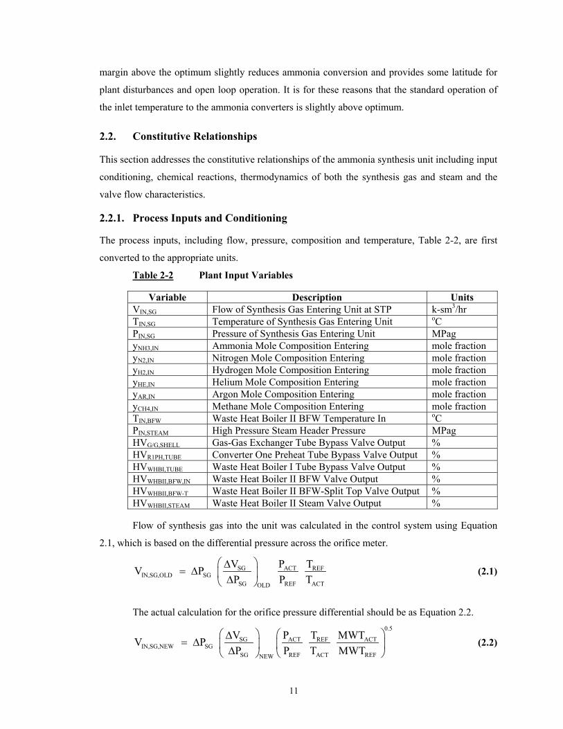
The process inputs, including flow, pressure, composition and temperature, Table 2-2, are first
converted to the appropriate units.
Table 2-2 Plant Input Variables
Variable Description Units VIN,SG Flow of Synthesis Gas Entering Unit at STP k-sm3/hr TIN,SG Temperature of Synthesis Gas Entering Unit oC PIN,SG Pressure of Synthesis Gas Entering Unit MPag yNH3,IN Ammonia Mole Composition Entering mole fraction yN2,IN Nitrogen Mole Composition Entering mole fraction yH2,IN Hydrogen Mole Composition Entering mole fraction yHE,IN Helium Mole Composition Entering mole fraction yAR,IN Argon Mole Composition Entering mole fraction yCH4,IN Methane Mole Composition Entering mole fraction TIN,BFW Waste Heat Boiler II BFW Temperature In oC PIN,STEAM High Pressure Steam Header Pressure MPag HVG/G,SHELL Gas-Gas Exchanger Tube Bypass Valve Output % HVR1PH,TUBE Converter One Preheat Tube Bypass Valve Output % HVWHBI,TUBE Waste Heat Boiler I Tube Bypass Valve Output % HVWHBII,BFW,IN Waste Heat Boiler II BFW Valve Output % HVWHBII,BFW-T Waste Heat Boiler II BFW-Split Top Valve Output % HVWHBII,STEAM Waste Heat Boiler II Steam Valve Output %
Flow of synthesis gas into the unit was calculated in the control system using Equation
2.1, which is based on the differential pressure across the orifice meter.
SG ACT REFIN,SG,OLD SG
SG REF ACTOLD
V P TV P P P T
∆= ∆ ∆
(2.1)
The actual calculation for the orifice pressure differential should be as Equation 2.2. 0.5
SG ACT ACTREFIN,SG,NEW SG
SG REF ACT REFNEW
V P MWTTV P P P T MWT
∆= ∆ ∆
(2.2)

12
Using Equations 2.1 and 2.2, the actual flow of synthesis gas entering the unit is
corrected as follows. Equation 2.4 is used to convert the flow rate from volumetric to mass. 0.5
SG SG ACT ACTREFIN,SG,CORR IN,SG,OLD
SG SG ACT REF REFOLD NEW
P V T MWTPV V V P P T MWT
∆ ∆= ∆ ∆
(2.3)
IN,SG IN,SG,CORR SG,IN,STP1000M V 3600
ρ= (2.4)
The operating pressure is calculated for the process gas in each vessel, using inlet
conditions and assuming a pressure drop of 0.1 MPa across each reactor bed. Inlet compositions
are normalized.
R1B1 IN,SG RXN ATMP P - P + P= ∆ (2.5)
R1B2 R1B1 RXNP P - P= ∆ (2.6)
R2 R1B2 RXNP P - P= ∆ (2.7)
2.2.2. Chemical Reactions
The conversion of hydrogen and nitrogen to ammonia is represented as:
2 2 31 3N + H NH2 2
⇔ (1.1)
This reaction is broken down into the elementary reactions in Equations 2.8 to 2.15[41].
Subscript (a) refers to the component absorbed onto the iron catalyst.
2 2(a)N +Fe N ⇔ (2.8)
2(a) (a) (a)N +Fe N +N ⇔ (2.9)
2 2(a)H +Fe H ⇔ (2.10)
2(a) (a) (a)H +Fe H H + ⇔ + (2.11)
(a) (a) (a)H N NH Fe + ⇔ + (2.12)
(a) (a) 2(a)H NH NH Fe + ⇔ + (2.13)
(a) 2(a) 3(a)H NH NH Fe + ⇔ + (2.14)
3(a) 3NH NH Fe ⇔ + (2.15)
13
2.2.3. Reaction Kinetics
The model studied in this thesis uses the Temkin-Pyshev[32] equation to describe the reaction
kinetics. The Temkin-Pyshev equation assumes that the rate of the reaction depends on the
chemisorption of nitrogen, Equation 2.9.
32
2
3 2
m 1 m23NHH
XN N 2 3NH H
R k k Volff
ff f
−
+ −
= −
(2.16)
The equilibrium constant of the ammonia reaction is described by the Equations 2.17 and
2.18[41].
3
2 2
2NH
P 3N H
kK ( ) = k_
fat equilibrium
f f+= (2.17)
12500 10 P 210027.366 1.42T T T
PK e − + + − + = (2.18)
The frequency factor for the reverse reaction is represented below in Equation 2.19. The
forward reaction frequency factor is calculated in Equation 2.20 based on equilibrium conditions
with a compensation term, fit to plant data.
( )k_E
R Tk_ = ko_ e∆
(2.19)
Pk = hx k_ K+ (2.20)
From these relationships, the reaction rates, Equations 2.21 to 2.23 are determined as
functions of the following variables using Equation 2.16.
XN,R1B1 R1B1 R1B1,OUT R1B1 R1B1 R1B1R = (P ,T ,y ,Vol ,hx )f (2.21)
XN,R1B2 R1B2 R1B2,OUT R1B2 R1B2 R1B2R = (P ,T ,y ,Vol ,hx )f (2.22)
XN,R2 R2 R2,OUT R2 R2 R2R = (P ,T ,y ,Vol ,hx )f (2.23)
Mole fractions are calculated from the reactor composition state variables, Equations 2.24
to 2.26.
i,R1B1i, R1B1
j,R1B1j
ny =
n∑ (2.24)
i,R1B2i, R1B2
j,R1B2j
ny =
n∑ (2.25)

14
i,R2i, R2
j,R2j
ny =
n∑ (2.26)
2.2.4. Heat of Reaction
The heat of reaction and the activation energy are calculated in Equations 2.27 and 2.28 based on
catalyst manufacturer information[41].
2 P
P
lnKHX = -R T T
δδ
(2.27a)
( )R= - -12500 T - 4200 P + 14.2 P TT
(2.27b)
k_ KE E (1 m) HX∆ = ∆ + − (2.28)
Equations 2.29 to 2.31 represent the heat of reaction for each converter bed as functions
of Equation 2.27.
R1B1 R1B1 R1B1HX = (T ,P )f (2.29)
R1B2 R1B2 R1B2HX = (T ,P )f (2.30)
R2 R2 R2HX = (T ,P )f (2.31)
2.2.5. Redlich-Kwong-Soave Equation of State
The enthalpies of the synthesis gas streams are calculated using the ideal gas enthalpy with a
residual enthalpy term. Due to the high pressure of the process (19 MPa), the residual enthalpy
contributes to about five percent of the total calculated enthalpy change.
( )OUT INhR -hRh
1000∆ = ∆ +y IGh (2.32)
PC = oPy C (2.33)
The ideal gas heat capacity is calculated from the Shomate[24] equation.
2 3mK mK mK 2
mK
T T TT
= + + + +oP
EC A B C D (2.34)
2 3 4mK mK mK
mKmK
T T T- T - 2 3 4 T
= + + + − + ∆o o298.15
B C D Eh h A F of,298h (2.35)
or
( ) ( ) ( )2 3mK,OUT mK,IN mK,OUT mK,IN
mK,OUT mK,IN
T T T T T T
2 3− −
∆ = − + + +A B C IGh

15
( )4mK,OUT mK,IN
mK,OUT mK,IN
T T 1 1 4 T T−
− −
D E (2.36)
Refer to Tables B-1 and B-2 in Appendix B for the gas properties and constants used to
calculate the process enthalpy changes.
The Redlich-Kwong-Soave[39] equation of state, Equation 2.37, is used to calculate the
synthesis gas compressibility, residual enthalpy and fugacity coefficients. Using a cubic form of
this equation, compressibility can be solved. Reference Equation 2.38.
( )( )RT aP -
c-b c c bυ υ υ=
+ + + + (2.37)
3 2 2( C) -(Z C) (Z C) (A-B-B )-A B 0Z + + + + ⋅ = (2.38)
The residual enthalpy found in Equation 2.39 is calculated using Maple®2. Calculation of
the fugacity coefficients[3] can be found in Equation 2.40.
0 11 bhR (Z-1) R T - (2 k k T) ln 1
2 b cυ = + + +
(2.39)
i ii i j i j
B A B 2 Bln -ln(Z C-B) (Z C-1)-C - y A A ln 1B B B A Z Cj
φ = + + + + + +
∑ (2.40)
Equations for the RKS constants and intermediate calculations used in Equations 2.39
and 2.40 can be found in Equations B.1 through B.20 of the Appendices.
Re-arranging the gas equation yields the gas density.
( )1 1000ρυ
= y MWT (2.41a)
( )P 1000Z R T
=
y MWT (2.41b)
Synthesis gas enthalpy, average heat capacity and average density calculations are listed
in Equations D.1 to D.16 of Appendix D as functions of Equations 2.32, 2.33 and 2.41.
2.2.6. Steam Calculations
Thermodynamic properties of steam are expressed mathematically by fitting equations to data
taken from the steam tables[37] over the temperature range considered. The waste heat boiler
(WHB) shell temperatures are used to determine the BFW and steam properties including the
saturation pressure, enthalpy, heat capacity and densities. These relationships are listed in
2 © 2000 Waterloo Maple Inc. Maple is a registered trademark of Waterloo Maple Inc.

16
Equations D.17 to D.21 of Appendix D. The changes in enthalpy across the WHB, attributed to
the steam system, are calculated in Equations 2.42 to 2.45.
( ) 3WHBI,SHELL WHBI,STEAM WHBI,STEAM CBD WHBI,BFW WHBI,BFW WHBII,SHELL-MIDH = M H M H M H 10−∆ + −
(2.42)
(( )WHBII,BFW-B WHBII,STEAM WHBII,STEAM WHBI,BFW CBD WHBII,BFW-MH M H M 2 M H ∆ = + +
) 3WHBII,BFW,IN WHBII,BFW,IN WHBII,BFW-M WHBII,BFW-TM H H H 10−− − ∆ − ∆ (2.43)
(WHBII,BFW-M WHBII,BFW-T WHBII,BFW,IN WHBII,BFW-M WHBI,BFW WHBII,BFW-BH M H fx M H∆ = +
( ) ) 3WHBII,BFW-T WHBII,BFW-M WHBII,BFW-B WHBII,BFW-MM fx M H 10−− + (2.44)
( )(WHBII,BFW-T WHBII,BFW-M WHBII,BFW-B WHBII,BFW-T WHBI,BFW CBDH fx M M M M∆ = + − −
( )WHBII,BFW-M WHBII,BFW-M WHBII,BFW-B WHBII,BFW-BH 1 fx M H+ −
( ) ) 3WHBII,BFW,IN WHBI,BFW CBD WHBII,BFW-TM M M H 10−− − − (2.45)
2.2.7. Heat Transfer
Heat transfer characteristics for each heat exchanger were provided by Saskferco[17]. Using these
values, the overall heat transfer is calculated for all heat exchangers. 6
G/G G/G G/G G/G m,G/GQ = U Ae f T 10−∆ (2.46)
6R1PH R1PH R1PH R1PH m,R1PHQ = U Ae f T 10−∆ (2.47)
6WHBI WHBI WHBI WHBI m,WHBIQ = U Ae f T 10−∆ (2.48)
6WHBII WHBII WHBII WHBII m,WHBIIQ = U Ae f T 10−∆ (2.49)
The mean temperature difference is based on the operating difference between the hot
side and the cold side of the exchanger.
WHBII,TUBE G/G,SHELL G/G,TUBE IN,SGm,G/G
(T -T ) (T -T )T
2+
∆ = (2.50)
R1B1 R1PH,TUBE R1PH,SHELL G/G,BYm,R1PH
(T -T ) (T -T )T
2+
∆ = (2.51)
R1B2 WHBI,SHELL WHB1,TUBE WHBII,BFW-Mm,WHBI
(T -T ) (T -T )T
2+
∆ = (2.52)
R2 WHBII,SHELL-B WHBII,TUBE WHBII,BFW,INm,WHBII
(T -T ) (T -T )T
2+
∆ = (2.53)
17
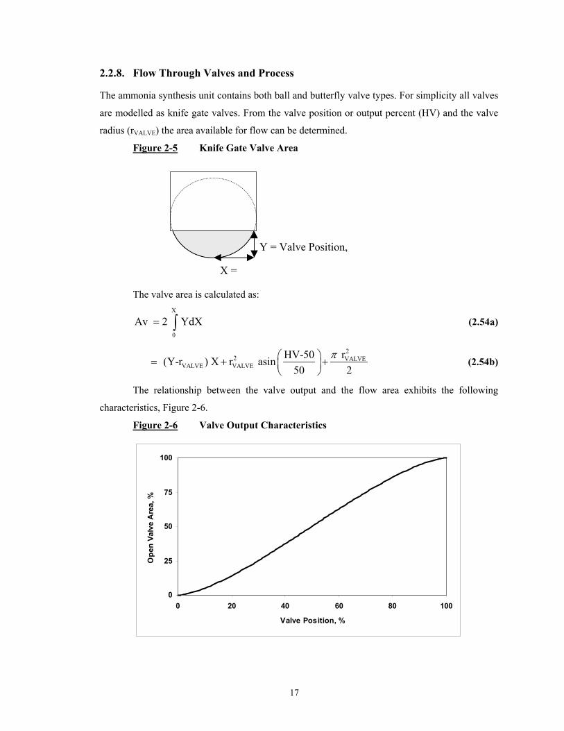
2.2.8. Flow Through Valves and Process
The ammonia synthesis unit contains both ball and butterfly valve types. For simplicity all valves
are modelled as knife gate valves. From the valve position or output percent (HV) and the valve
radius (rVALVE) the area available for flow can be determined.
Figure 2-5 Knife Gate Valve Area
The valve area is calculated as: X
0
Av 2 YdX = ∫ (2.54a)
22 VALVE
VALVE VALVE rHV-50 (Y-r ) X r asin
50 2π = + +
(2.54b)
The relationship between the valve output and the flow area exhibits the following
characteristics, Figure 2-6.
Figure 2-6 Valve Output Characteristics
0
25
50
75
100
0 20 40 60 80 100
Valve Position, %
Ope
n Va
lve
Are
a, %
Y = Valve Position,
X =

18
Available flow area functions, Equations D.22 to D.33, based on Equation 2.54, are listed
in Appendix D. Flows to each vessel are then calculated in Equations 2.55 through 2.66 for
synthesis gas and Equations 2.67 through 2.72 for BFW and steam.
IN,SGG/G,TUBE
MF =
R2y MWT (2.55)
IN,SG G/G,SHELLG/G,SHELL
G/G,SHELL G/G,BY
M AvF =
Av Av+INy MWT (2.56)
IN,SG G/G,BYG/G,BY
G/G,SHELL G/G,BY
M AvF =
Av Av+INy MWT (2.57)
IN,SG R1PH,TUBER1PH,TUBE
R1PH,TUBE R1PH,BY
M AvF =
Av Av+INy MWT (2.58)
IN,SG R1PH,BYR1PH,BY
R1PH,TUBE R1PH,BY
M AvF =
Av Av+INy MWT (2.59)
IN,SGR1PH,SHELL
MF =
R1B1y MWT (2.60)
IN,SGR1B1
MF =
INy MWT (2.61)
R1B2 R1PH,SHELLF = F (2.62)
IN,SG WHBI,TUBEWHBI,TUBE
WHBI,TUBE WHBI,BY
M AvF =
Av Av+R1B2y MWT (2.63)
IN,SG WHBI,BYWHBI,BY
WHBI,TUBE WHBI,BY
M AvF =
Av Av+R1B2y MWT (2.64)
IN,SGR2
MF =
R1B2y MWT (2.65)
IN,SGWHBII,TUBE
MF =
R2y MWT (2.66)
( )WHBI,BFW WHBI,BFW WHBII,BFW WHBI,BFWM = Av 2 g ht -ht (2.67)
WHBII,BFW,IN WHBII,BFW,IN WHBII,BFW,IN BFW,INM = Av vρ (2.68)
( )WHBI,STEAM STEAMWHBI,STEAM WHBI,STEAM WHBI,STEAM
WHBI,STEAM
2 P -PM = Avρ
ρ (2.69)
WHBII,BFW-TWHBII,BFW-T WHBII,BFW,IN
WHBII,BFW-T WHBII,BFW-B
AvM = M
Av Av+ (2.70)

19
WHBII,BFW-BWHBII,BFW-B WHBII,BFW,IN
WHBII,BFW-T WHBII,BFW-B
AvM = M
Av Av+ (2.71)
( )WHBII,STEAM STEAMWHBII,STEAM WHBII,STEAM WHBII,STEAM
WHBII,STEAM
2 P -PM = Avρ
ρ (2.72)
2.2.9. Vessel Hold-Up
Hold-up in each vessel is determined from the vessel volume[17] and gas density. For calculations
involving a bypass valve, the mix area is assumed to occur over one metre length of pipe. Again
density calculations are expressed as a function of Equation 2.41.
G/G,TUBE G/G,TUBE HOLDUPG/G,TUBE
Vol gxG =
ρ
R2y MWT (2.73)
G/G,SHELL G/G,SHELL HOLDUPG/G,SHELL
Vol gxG =
ρ
INy MWT (2.74)
( )2G/G,SHELL MIX G/G,BY1 G/G,BY2
G/G,BY
r L 0.5 G =
π ρ ρ∆ +
INy MWT (2.75)
R1PH,TUBE R1PH,TUBE HOLDUPR1PH,TUBE
Vol gxG =
ρ
INy MWT (2.76)
( )R1PH,BY R1PH,BY1 R1PH,BY2R1PH,BY
Vol 0.5 G =
ρ ρ+
INy MWT (2.77)
R1PH,SHELL R1PH,SHELL HOLDUPR1PH,SHELL
Vol gxG =
ρ
R1B1y MWT (2.78)
VOID R1B1 R1B1 HOLDUPR1B1
f Vol gxG = ρ
R1B1y MWT (2.79)
VOID R1B2 R1B2 HOLDUPR1B2
f Vol gxG = ρ
R1B2y MWT (2.80)
WHBI,TUBE WHBI,TUBE HOLDUPWHBI,TUBE
Vol gxG =
ρ
R1B2y MWT (2.81)
( )2WHBI,TUBE MIX WHBI,B-1 WHBI,B-2
WHBI,B
r L 0.5 G =
π ρ ρ∆ +
R1B2y MWT (2.82)
VOID R2 R2 HOLDUPR2
f Vol gxG = ρ
R2y MWT (2.83)
WHBII,TUBE WHBII,TUBE HOLDUPWHBII,TUBE
Vol gxG =
ρ
R2y MWT (2.84)

20
WHBI,SHELLWHBI,SHELL WHBI,SHELL WHBI,SHELL WHBI,SHELL
LGw = Vol Ax ht
100
+
WHBI,BFW HOLDUP gxρ (2.85)
WHBII,SHELL-B WHBII,SHELL-B WHBII,BFW-B HOLDUPGw = Vol gxρ (2.86)
WHBII,SHELLWHBII,SHELL-M WHBII,SHELL-T WHBII WHBII
LGw = Vol Ax ht
100
+
WHBII,BFW-M HOLDUPgx 0.95 ρ (2.87)
WHBII,SHELLWHBII,SHELL-T WHBII,SHELL-T WHBII WHBII
LGw = Vol Ax ht
100
+
WHBII,BFW-M HOLDUPgx 0.05 ρ (2.88)
2.3. Material & Energy Balances
Process dynamics are modelled for each vessel in the unit. Most of the process ordinary
differential equations (ODE) are based on an energy balance[7] around the vessel considered, as
expressed in Equation 2.89. Mass balances around the converters and the WHBs are also
developed. The standard ODE formats for the converters and vessel levels are given by Equations
2.90 and 2.91.
IN OUT
P Holdup
E - EdT dt C G
= (2.89)
ii,IN i, RXN i,OUT
dn n n -ndt
= + (2.90)
( )jj
MdL 100dt Ax ht ρ
=∑
(2.91)
Equations 2.89 to 2.91 are adapted to the ammonia process under consideration. The state
variables for each vessel can be found in Equations 2.92 to 2.112.
( )G/G,TUBE G/G G/G,TUBE G/G,TUBE
G/G,TUBE P,G/G,TUBE
d T - Q -F h =
dt G C∆ (2.92)
( )G/G,SHELL G/G G/G,SHELL G/G,SHELL
G/G,SHELL P,G/G,SHELL
d T Q - F h =
dt G C∆ (2.93)
( )( )
G/G,BY G/G,BY G/G,BY1 G/G,SHELL G/G,BY2
G/G,BY P,G/G,BY1 P,G/G,BY2
d T F h F h =
dt G C C 0.5− ∆ − ∆
+ (2.94)

21
( )R1PH,TUBE R1PH R1PH,TUBE R1PH-1 R1PH,TUBE
R1PH,TUBE P,R1PH,TUBE
d T Q -F f h =
dt G C∆ (2.95)
( )R1PH,BY R1PH,BY R1PH,BY1 R1PH,TUBE R1PH,BY2
R1PH,BY P,R1PH,BY1 P,R1PH,BY2
dT F h F h =
dt G C C 0.5− ∆ − ∆
+ (2.96)
( )R1PH,SHELL R1PH R1PH,SHELL R1PH-2 R1PH,SHELL
R1PH,SHELL P,R1PH,SHELL
d T -Q - F f h =
dt G C∆ (2.97)
( )XN,R1B1R1B1
R1B1 R1B13R1B1
R1B1 P,R1B1
RHX - F hd T 2 x10 3600 = dt G C
∆ (2.98)
( )XN,R1B2R1B2
R1B2 R1B23R1B2
R1B2 P,R1B2
RHX - F hd T 2x10 3600 = dt G C
∆ (2.99)
R1B1IN R1B1 XN,R1B1 R1B1 R1B2
d(n ) =y F rxn_coeff R y F dt
+ − (2.100)
R1B2R1B1 R1B2 XN,R1B2 R1B2 R2
d(n ) =y F rxn_coeff R y F dt
+ − (2.101)
( )WHBI,TUBE WHBI WHBI,TUBE WHBI,TUBE
WHBI,TUBE P,WHBI,TUBE
d T -Q -F h =
dt G C∆ (2.102)
( )WHBI,BY WHBI,BY WHB,BY1 WHBI,TUBE WHBI,BY2
WHBI,BY P,WHBI,BY2 P,WHBI,BY2
dT F h F h =
dt G C C 0.5− ∆ − ∆
+ (2.103)
( )WHBI,SHELL WHBI WHBI,SHELL
WHBI,SHELL P,WHBI,BFW
d T Q H =
dt Gw C− ∆ (2.104)
( )WHBI,SHELL WHBI,BFW CBD WHBI,STEAM
WHBI WHBI WHBI,BFW
d L M - M - M 100
dt Ax ht ρ= (2.105)
R2R1B2 R2 XN,R2 R2 WHBII,TUBE
d(n ) =y F rxn_coeff R y F dt
+ − (2.106)
( )XN,R2R2
R2 R23R2
R2 P,R2
RHX - F hd T 2x10 3600 = dt G C
∆ (2.107)
( )WHBII,TUBE WHBII WHBII,TUBE WHBII,TUBE
WHBII,TUBE P,WHBII,TUBE
d T -Q -F h =
dt G C∆ (2.108)
( )WHBII,SHELL-B WHBII WHBII,SHELL-B
WHBII,SHELL-B P,WHBII,BFW-B
d T Q H =
dt Gw C− ∆ (2.109)

22
( )WHBII,SHELL-M WHBII,SHELL-M
WHBII,SHELL-M P,WHBII,BFW-M
d T H =
dt Gw C∆ (2.110)
( )WHBII,SHELL-T WHBII,SHELL-T
WHBII,SHELL-T P,WHBII,BFW-T
d T H =
dt Gw C∆ (2.111)
( )WHBII,SHELL WHBII,BFW,IN WHBI,BFW CBD WHBII,STEAM
WHBII WHBII WHBII,BFW-M
d L M - M - M - M 100
dt Ax ht ρ= (2.112)
2.4. Model Implementation
In an effort to design optimization and control applications for the converter, the process is
modelled in Matlab®3 version 5.3 and Simulink®3 version 3.0.
Process ODEs are implemented using Matlab standard s-functions. Programming is done
in a modular fashion for each vessel. This is done to allow for increased flexibility and ease of
use for program testing and modifications. The modular programs are then linked together in
Simulink using subsystem blocks. It is also in Simulink that the process inputs, disturbances and
time delays are introduced into the model. An overview of the model can be found in Appendix
C, Figure C-1.
2.5. Model Validation
Model validation is based on existing plant data encompassing process changes. Two data sets
were collected from the plant. The first data set, used to fit steady-state model predictions to plant
data, is based on twelve hour shift averages for the month of March 1999. The second data set,
taken from February 1999, is used to validate these results. This data set excludes data from
February 24th and 25th, since the ammonia plant was not in operation during this time period.
The parameter estimates found using plant data from March are listed in Table 2-3.
3 © 1999 The MathWorks, Inc. Matlab and Simulink are registered trademarks of The MathWorks, Inc.

23
Table 2-3 Fitted Parameters
Parameters Description Value Units fG/G Gas-Gas Heat Transfer Correction Term 1.1807 -- fR1PH-1 R1 Preheat Heat Transfer Correction Term 0.9669 -- fR1PH-2 R1 Preheat Heat Transfer Correction Term 1.0603 -- fWHBI WHB I Heat Transfer Correction Term 0.9321 -- fWHBII WHB II Heat Transfer Correction Term 1.0270 -- hxR1B1 R1B1 Forward Reaction Parameter Estimate 1.5976 -- hxR1B2 R1B2 Forward Reaction Parameter Estimate 1.3337 -- hxR2 R2 Forward Reaction Parameter Estimate 1.2604 -- vBFW,IN BFW Velocity to WHB II 2.3907 m/s MCBD WHB I and II Continuous Blowdown 3.5 kg/s gxHOLDUP Vessel Hold-up Correction Term 10 -- These values can be classified as follows.
1. Heat Transfer Correction Terms
Parameters f are calculated using previously defined equations and averaging
results for the month of March.
2. Catalyst Effectiveness Parameters
Parameters hx are fit by minimizing the sum of the square of the error between
the model predictions and the process data. Characteristics of this method are
described in detail in Chapter 3. Average results for the month of March are used
to validate model performance.
3. Average Process Operation
Parameters vBFW,IN and MCBD are calculated based on the average operation for
March.
4. Dynamic Model Characteristics
A parameter, gxHOLDUP, is introduced to compensate for changes in energy in the
vessel that are not modelled. For example, the first converter bed has a residence
time of three seconds based on its gas hold-up capacity. However, the integral
time of the exiting temperature is notably larger. This difference is attributed to
changes in the stored energy of the vessel (eight inch wall thickness) and the iron
catalyst (modelled as 64% of the vessel volume[41]).
Other factors commonly fit to experimental data can be found in Table 2-4. In this case,
values from catalyst suppliers are used.
24
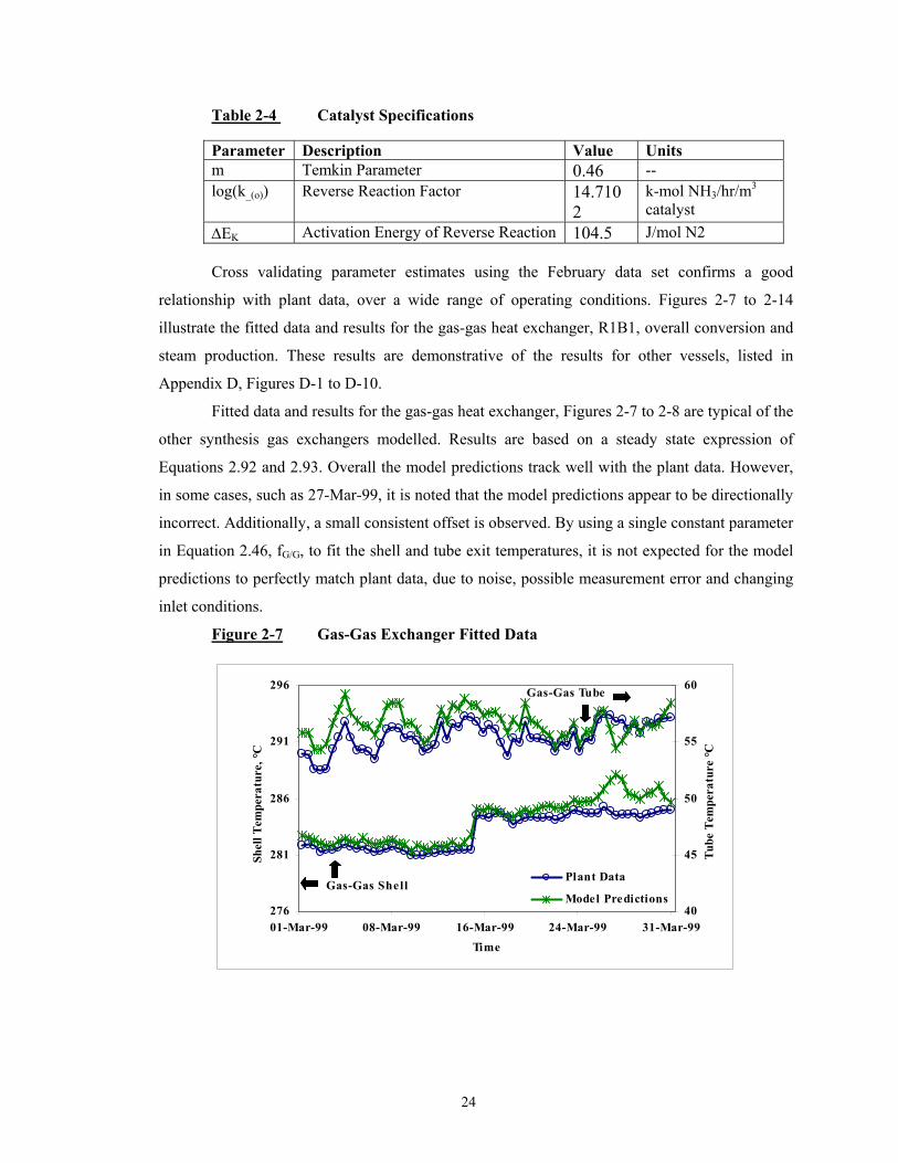
Table 2-4 Catalyst Specifications
Parameter Description Value Units m Temkin Parameter 0.46 -- log(k_(o)) Reverse Reaction Factor 14.710
2 k-mol NH3/hr/m3 catalyst
∆EK Activation Energy of Reverse Reaction 104.5 J/mol N2 Cross validating parameter estimates using the February data set confirms a good
relationship with plant data, over a wide range of operating conditions. Figures 2-7 to 2-14
illustrate the fitted data and results for the gas-gas heat exchanger, R1B1, overall conversion and
steam production. These results are demonstrative of the results for other vessels, listed in
Appendix D, Figures D-1 to D-10.
Fitted data and results for the gas-gas heat exchanger, Figures 2-7 to 2-8 are typical of the
other synthesis gas exchangers modelled. Results are based on a steady state expression of
Equations 2.92 and 2.93. Overall the model predictions track well with the plant data. However,
in some cases, such as 27-Mar-99, it is noted that the model predictions appear to be directionally
incorrect. Additionally, a small consistent offset is observed. By using a single constant parameter
in Equation 2.46, fG/G, to fit the shell and tube exit temperatures, it is not expected for the model
predictions to perfectly match plant data, due to noise, possible measurement error and changing
inlet conditions.
Figure 2-7 Gas-Gas Exchanger Fitted Data
276
281
286
291
296
01-Mar-99 08-Mar-99 16-Mar-99 24-Mar-99 31-Mar-99Time
Shel
l Tem
pera
ture
, °C
40
45
50
55
60
Tube
Tem
pera
ture
°C
Plant Data
Model PredictionsGas-Gas Shell
Gas-Gas Tube

25
Figure 2-8 Gas-Gas Exchanger Results
278
283
288
293
298
01-Feb-99 07-Feb-99 14-Feb-99 21-Feb-99 28-Feb-99Time
Shel
l Tem
pera
ture
, °C
42
47
52
57
62
Tube
Tem
pera
ture
, °C
Plant Data
Model Predictions
Gas-Gas Shell
Gas-Gas Tube
Three parameters, hxR1B1, hxR1B2 and hxR2 in Equations 2.21 to 2.23 are used to fit the exit
temperature of the three conversion beds and the overall ammonia conversion.
Conversion temperature results for R1B1, based on Equation 2.98, can be observed in
Figures 2-9 and 2-10. Unlike the other reactor beds, R1B1 does not have a measured exit
temperature. Therefore four bed temperatures are averaged to fit the model predictions. Since the
majority of the ammonia conversion occurs in this bed, the largest temperature rise (about +133
°C) is observed across R1B1.
Figure 2-9 Converter One Bed One Fitted Data
492
500
508
516
524
01-Mar-99 08-Mar-99 16-Mar-99 23-Mar-99 31-Mar-99Time
R1B
1 C
onve
rsio
n Te
mpe
ratu
re, °
C
Plant DataModel Predictions

26
Figure 2-10 Converter One Bed One Results
492
500
508
516
524
01-Feb-99 07-Feb-99 14-Feb-99 21-Feb-99 28-Feb-99Time
R1B
1 C
onve
rsio
n Te
mpe
ratu
re, °
C
Plant DataModel Predictions
Total ammonia conversion is illustrated in Figures 2-11 and 2-12. The most notable
characteristic in these figures is the sudden jump in the plant’s ammonia conversion from 13.9 %
to 15.3 % between 25-Mar-99 to 27-Mar-99. Possible reasons why the model does not predict this
spike are discussed in Section 2.6.
Figure 2-11 Overall Ammonia Conversion Fitted Data
12
13
14
15
16
01-Mar-99 08-Mar-99 16-Mar-99 24-Mar-99 31-Mar-99Time
Am
mon
ia C
onve
rsio
n, %
Plant DataModel Predictions

27
Figure 2-12 Overall Ammonia Conversion Results
12
13
14
15
16
01-Feb-99 07-Feb-99 14-Feb-99 21-Feb-99 28-Feb-99Time
Am
mon
ia C
onve
rsio
n, %
Plant Data
Model Predictions
Lastly results from the steam system are presented in Figures 2-13 and 2-14. Data from
WHB I and WHB II are used to determine the correction terms for the overall exchanger heat
transfer, fWHBI and fWHBII, in Equations 2.48 and 2.49. The average BFW velocity, vBFW,IN, and the
average continuous blow down (CBD), MCBD, for the month of March are used. Steam production
offset for the month of February is largely attributed to using average BFW and CBD rates.
Difficulties with directional predictions are a carry-over of problems in modelling upstream
vessels.
Figure 2-13 Waste Heat Boiler Steam Fitted Data
92
97
102
107
112
01-Mar-99 08-Mar-99 16-Mar-99 24-Mar-99 31-Mar-99Time
Stea
m P
rodu
ctio
n, to
nne/
hr
Plant DataModel Predictions

28
Figure 2-14 Waste Heat Boiler Steam Production Results
92
97
102
107
112
01-Feb-99 08-Feb-99 16-Feb-99 24-Feb-99Time
Stea
m P
rodu
ctio
n, to
nne/
hr
Plant DataModel Predictions
2.6. Discussion
In consideration of the nonideal thermodynamic behaviour and kinetics for the synthesis of
ammonia, a nonlinear dynamic model of the process is developed. The steady-state performance
of the model is compared to existing operations, where eight correction terms are fit using twelve
plant measurements.
In general, model results provide an adequate fit to plant data over a wide range of
operating conditions, based on 12 hour shift averages. However, a significant discrepancy is
observed between plant data and model predictions for ammonia conversion around 27-Mar-01.
Inspection of plant disturbances such as synthesis gas feed, Figure 2-15, suggests that the process
may be diffusion limited at higher feed rates.

29
Figure 2-15 Synthesis Gas Feed
700
740
780
820
860
01-Mar-99 08-Mar-99 16-Mar-99 24-Mar-99 31-Mar-99Time
Synt
hesis
Gas
Fee
d (c
orre
cted
), k-
sm3/
hr
The sudden increase in the H/N ratio at this time, Figure 2-16, may also contribute to
model inaccuracy. Interestingly, model results of the rising H/N ratio are contradictory to
literature that indicates a negative impact on ammonia conversion at H/N ratios above 2.8[41].
Figure 2-16 Synthesis Gas Hydrogen to Nitrogen Ratio in Feed Stream
2.5
3.0
3.5
4.0
4.5
01-Mar-99 08-Mar-99 16-Mar-99 24-Mar-99 31-Mar-99Time
H/N
Rat
io, m
ole/
mol
e
In the converters, the model predicts a sudden increase in the conversion temperature on
9-Mar-99, where none had occurred, Figure 2-9. A sudden drop in inert composition in the feed
stream, Figure 2-17, and a rise in the ammonia recycle, Figure 2-18, are also observed at this
time. This suggests that a constant catalyst effectiveness term does not adequately account for
large changes in process operation. Dynamic update of this parameter is explored in Chapter 3.
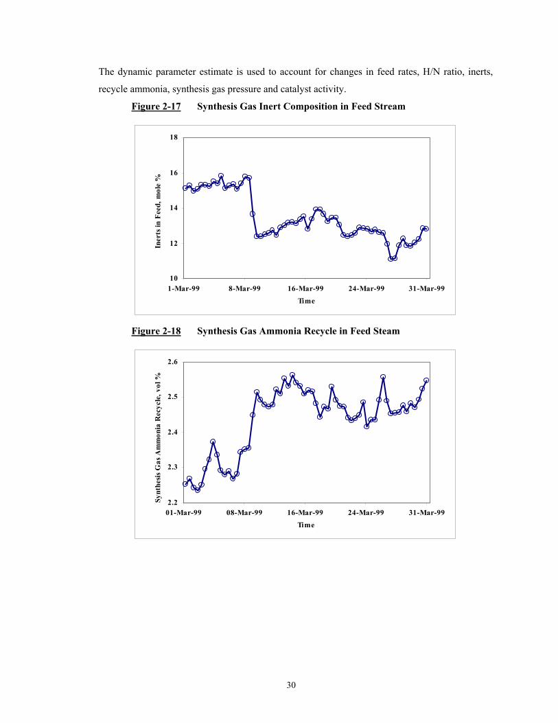
30
The dynamic parameter estimate is used to account for changes in feed rates, H/N ratio, inerts,
recycle ammonia, synthesis gas pressure and catalyst activity.
Figure 2-17 Synthesis Gas Inert Composition in Feed Stream
10
12
14
16
18
1-Mar-99 8-Mar-99 16-Mar-99 24-Mar-99 31-Mar-99Time
Iner
ts in
Fee
d, m
ole
%
Figure 2-18 Synthesis Gas Ammonia Recycle in Feed Steam
2.2
2.3
2.4
2.5
2.6
01-Mar-99 08-Mar-99 16-Mar-99 24-Mar-99 31-Mar-99
Time
Synt
hesis
Gas
Am
mon
ia R
ecyc
le, v
ol %

31
CHAPTER 3
PARAMETER UPDATES USING HISTORICAL DATA
In an operating plant the catalyst activity and the heat transfer coefficients change due to fouling
and variations in process conditions. Knowledge of these parameters and how they vary is an
important step in moving the process to its optimal operating conditions[35].
In Chapter 2, several parameters are introduced to fit the model to the process. In this
chapter, different ways of using steady-state historical data to update the catalyst effectiveness
parameters are investigated. Update of the heat transfer correction terms is not addressed here.
To account for changing catalyst activity and changing equilibrium conditions, an
appropriate model parameter must be identified first. Catalyst manufacturers offer specifications
relating to their catalyst, as listed in Table 2-4. The possibility of using these values is evaluated.
Other possible catalyst effectiveness parameters are also considered. In choosing a suitable
parameter, the impact on the reaction curve is evaluated.
Several techniques for updating the parameter identified are studied. These techniques are
based on variations of the least squares method, which is the classic approach to estimate model
coefficients[11]. The intent is to identify the pros and cons of each technique. Results of each
technique are expressed in relation to the estimation error, the ability to reject process noise
and/or instrumentation error, and the feasibility of each method based on computer resources
required to solve the problem. Historical data from Saskferco, based on 12 hour shift averages are
used. Due to the fast dynamics of this nonlinear process relative to the process disturbance
frequency, it is assumed that the historical process data represents steady-state operation.
Ultimately a recommended approach for parameter updates, specific to the process considered, is
offered. Correlations between the estimation parameters and process input conditions are
investigated and commented on.
3.1. Parameter Selection
The process simulated in Chapter 2 uses the Temkin-Pyshev equation to describe the reaction
rate. The catalyst activity parameter to be identified is ultimately incorporated into Equation 2.16.
This section considers the published catalyst manufacturer parameters and alternatively a
correction factor on the forward reaction as possible candidates to fit model results to plant data.

32
32
2
3 2
m 1 m23NHH
XN N 2 3NH H
R k k Volff
ff f
−
+ −
= −
(2.16)
Manufacturer catalyst parameters include the following:
1. Temkin constant, m,
2. Frequency factor for the reverse reaction, ko_ and
3. Activation energy constant ∆Ek, for the reverse reaction
To gain an understanding of the impact of these constants on the model, the optimal value
of these parameters is calculated using a single data set. Published and calculated results are listed
in Table 3-1. The impact of modifying these parameters on the reaction curve can be viewed in
Figure 3-1 and Table 3-2. Most notable, changing these parameters impacts the maximum
potential ammonia production with a reduced temperature at which optimal conversion is
achieved.
Table 3-1 Catalyst Manufacturer Parameter Calculations for R1B1
m log(ko_) kJ/kmol NH3/hr/m3
∆EK kJ/mol N2
Published Values 0.46-0.75 14.7102 104.5-110.8 Calculated m 0.50 14.7102 104.5 Calculated log(ko_) 0.46 15.0917 104.5 Calculated ∆EK 0.46 14.7102 98.8 Figure 3-1 Impact of Changing Model Parameters on Ammonia Reaction
1.0
2.5
4.0
5.5
7.0
8.5
10.0
300 350 400 450 500
R1B1 Inlet Temperature, oC
Am
mon
ia C
onve
rsio
n, %
Base Casem=0.46
∆EK=104.5ko_=1014.7102
m=0.50
ko_=1015.0917
∆EK=98.8

33
Table 3-2 Model Parameters with Calculated Optimum Temperature
m log(ko_) kJ/kmol NH3
/hr/m3
∆EK kJ/mol N2
R1B1 TOPT
oC
R1B1 Conversion
% 0.46 14.7102 104.5 399 6.380.50 14.7102 104.5 325 8.760.46 15.0917 104.5 338 8.390.46 14.7102 98.8 332 8.49
The large shift in the reaction curve, observed in Figure 3-1, is considered erroneous and
update of the manufacturer parameters is dropped due to its infeasibility. Since this thesis only
considers operation within a small range of the reaction curve (within approximately 20 oC for
R1B1), it is decided to use published parameters based on the assumption that these values were
determined from a broader range of conversion temperatures.
Chapter 2 introduced a term referred to as the catalyst effectiveness parameter, defined in
Equation 2.20. The correction factor, hx, is used to fit the equilibrium forward reaction rate to the
actual forward reaction rate. It is noted that the forward reaction is considered the rate-limiting
step.
Pk = hx k_ K+ (2.20)
Subsequent discussion on parameter update techniques and results uses three parameters,
hxR1B1, hxR1B2 and hxR2 to fit the process model to measured process variables. The remainder of
this chapter considers update of hx as a dynamic value, sensitive to process disturbances and
changes to input conditions.
3.2. Least Squares Regression Formulation
The least squares approach yields a solution that minimizes the problem’s objective function[6],
expressed as a function of the problem error. Two parameter update methods are evaluated in an
attempt to find the approach best suited to the ammonia synthesis parameter update problem.
These approaches include the sum of squares and recursive least squares. Both methods are based
on least squares regression techniques.
The sum of squares is a common approach to estimate model coefficients. The second
method, recursive least squares, uses difference equations to calculate the catalyst parameters.
The weighting matrix is calculated from the variation in error of the model variables.
The sum of squares algorithm compares results using a single data set and multiple data
sets to update the parameter. Multiple data sets potentially increase the robustness of the
parameter estimation problem by rejecting or reducing the impact of erroneous or noisy signals.

34
However, the use of too many data sets dampens the response to current operating conditions. As
a compromise, four data sets are used to evaluate this criterion. Four data sets were chosen to
allow the estimator to respond to current operating conditions, while weighing historical trends.
The model variables and parameters for the update problem are defined in Equations 3.1
to 3.3. y refers to the measured plant variables, scaled appropriately. These variables include the
conversion temperature into each reactor bed and the total ammonia production. y are the
estimated variables. u are the parameters to be manipulated to meet the objective function.
( )
R1B1,PLANT
R1B2,PLANT
R2,PLANT
NH3,PLANT
TT
= TM 10
y (3.1)
( )
R1B1,CALC
R1B2,CALC
R2,CALC
NH3,CALC
TT
ˆ = TM 10
y (3.2)
R1B1
R1B2
R2
hx = hx
hx
u (3.3)
The calculated total ammonia production is based on the sum of ammonia produced in
each converter, Equation 3.4.
( ) 3NH3,CALC XN,R1B1,CALC XN,R1B2,CALC XN,R2,CALC NH3M = R + R + R MWT 10− (3.4)
3.2.1. Sum of Squares
The first formulation is based on minimizing the sum of the squared errors of the three reactor
bed temperatures and ammonia production using a single, stationary sample period. The problem
solution in this case does not depend on the results of preceding time periods. The objective
function is posed in Equation 3.5, with 123 equality constraints referenced in Equation 3.6.
Dependent variables referenced in Equation 3.6 are listed in Table E-1 of Appendix E.
Case 1a
Minimize:
( )4
2i i
i=1
ˆe( , ) = y -y∑y u (3.5)
Subject to:

35
jh ( ) = 0 j = 1, 2, ... 123y,u (3.6)
To ensure reliable and efficient solution of the parameter estimation problem, variables
are scaled and equations manipulated to eliminate decision and dependent variables from
equation denominators. Constraint equalities use the equations specified in Chapter 2. Deviations
from this are as follows.
1. Converter temperatures and reaction rates are solved using steady-state mass
and energy balances.
2. For convenience, several intermediate calculations are introduced. These
variables are listed in Section E.2 of Appendix E.
Extending Case 1a to include multiple data sets, the objective function and constraint
equalities are reposed in Case 1b as shown in Equations 3.7 and 3.8.
Case 1b
Minimize:
( )0 4
2n i i n
n=-3 i=1
ˆe( , ) = y(t ) -y (t )
∑ ∑y u (3.7)
Subject to:
n,jh ( ) = 0 n = -3, -2, ... 0; j = 1, 2 ... 123y,u (3.8)
Where: n is the sample period, based on 12 hour shift averages (e.g. at t0 = 25-Mar-99 7
AM, t−1 = 24-Mar-99 7 PM, t−2 = 24-Mar-99 7 AM, t−3 = 23-Mar-99 7 PM.)
3.2.2. Recursive Least Squares
The recursive least squares method is similar to Case 1, in that it uses the sum of the squared
error, but with a weighting matrix based on knowledge of the process. Additionally, as a recursive
function, results depend on the results of preceding solutions. Equations 3.9 to 3.10 outline the
process. Variables are expressed as difference equations, depending on the values of previous
time periods to determine the predicted operation for comparison to measured plant variables.
ˆ = y Φ u (3.9)
( , ) ∂=
∂F y u
uΦ (3.10)
The error between the measured and estimated outputs is expressed in Equation 3.11.
Equation 3.11 is the cost function to be minimized. From this basis, u can be evaluated by solving
the Jacobian of Equation 3.11. This yields Equation 3.12[36]. 2 T T = = ( - ) ( - )e e e y u y uΦ Φ (3.11)

36
( )-1T = u yΦ Φ Φ (3.12)
Introducing a weighting matrix in the objective function, the recursive least squares
problem is posed in Equation 3.13[36].
Case 2
Minimize: 2 T T = = ( - ) ( - )e e W e y u W y uΦ Φ (3.13)
The parameter update calculation then becomes Equation 3.14. The weighting matrix is
set to the inverse of the covariance matrix, Equations 3.15 to 3.16.
( )-1T = u W W yΦ Φ Φ (3.14)
2
1 diag( )
=Wσ
(3.15)
2 var( )=σ e (3.16)
The parameter update matrix, Φ, is a complex function of changing process inputs and
outputs. It is recalculated in each parameter update calculation based on the steady-state mass and
energy balances around each bed. In determining the matrix function, the change in gas activity,
compression factors and residual enthalpies with respect to the update parameters is assumed
relatively negligible.
( ) ( ) ( )
( ) ( ) ( )
( ) ( ) ( )
( ) ( )3 3 3
R1B1,CALC R1B1,CALC R1B1,CALC
R1B1 R1B2 R2
R1B2,CALC R1B2,CALC R1B2,CALC
R1B1 R1B2 R2
R2,CALC R2,CALC R2,CALC
R1B1 R1B2 R2
NH ,CALC NH ,CALC NH ,CALC
R1B1 R1B2
T T Thx hx hx
T T Thx hx hx
T T Thx hx hx
M M Mhx hx h
∂ ∂ ∂∂ ∂ ∂
∂ ∂ ∂∂ ∂ ∂
=∂ ∂ ∂∂ ∂ ∂
∂ ∂ ∂
∂ ∂ ∂
Φ
( )R2x
(3.17)
Since the above equations are all expressed as difference variables, a judicious starting
point is required. The absolute value of the parameter updates depends on the previous
calculations. At time zero, un uses the calculated value from the sum of squares approximation,
for one sample period.
( ) 1T Tn n-1
−= +u u W W yΦ Φ Φ (3.18)
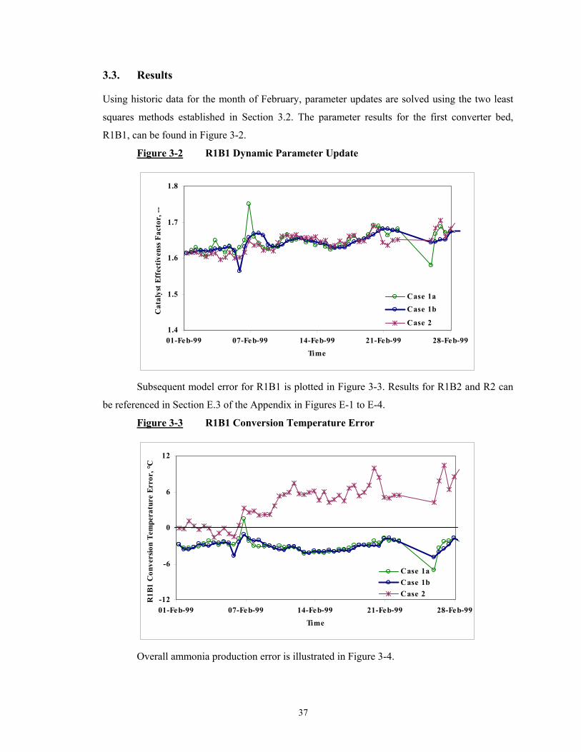
37
3.3. Results
Using historic data for the month of February, parameter updates are solved using the two least
squares methods established in Section 3.2. The parameter results for the first converter bed,
R1B1, can be found in Figure 3-2.
Figure 3-2 R1B1 Dynamic Parameter Update
1.4
1.5
1.6
1.7
1.8
01-Feb-99 07-Feb-99 14-Feb-99 21-Feb-99 28-Feb-99Time
Cat
alys
t Eff
ectiv
enss
Fac
tor,
--
Case 1aCase 1b
Case 2
Subsequent model error for R1B1 is plotted in Figure 3-3. Results for R1B2 and R2 can
be referenced in Section E.3 of the Appendix in Figures E-1 to E-4.
Figure 3-3 R1B1 Conversion Temperature Error
-12
-6
0
6
12
01-Feb-99 07-Feb-99 14-Feb-99 21-Feb-99 28-Feb-99Time
R1B
1 C
onve
rsio
n Te
mpe
ratu
re E
rror
, °C
Case 1aCase 1bCase 2
Overall ammonia production error is illustrated in Figure 3-4.

38
Figure 3-4 Overall Ammonia Production Error
-4
-2
0
2
4
01-Feb-99 07-Feb-99 14-Feb-99 21-Feb-99 28-Feb-99Time
NH
3 Pro
duct
ion
Erro
r, to
nne/
hr
Case 1aCase 1b
Case 2
Results are summarized in Table 3-3.
Table 3-3 Variable and Parameter Results for Parameter Update Problem
Case 1a Case 1b Case 2
hxR1B1,STD 0.028 0.022 0.025
hxR1B2,STD 0.042 0.027 0.020
hxR2,STD 0.056 0.036 0.013
TR1B1,ERR,AVG (oC) -2.9 -3.0 4.1
TR1B2,ERR,AVG (oC) -2.8 -2.9 0.7
TR2,ERR,AVG (oC) -2.8 -2.8 0.8
MNH3,ERR,AVG (tonne/hr) 0.08 0.04 0.004
TR1B1,ERR,RNG (oC) -7.0 to 1.5 -4.9 to –1.1 -1.6 to 10.4
TR1B2,ERR,RNG (oC) -6.8 to 1.5 -4.5 to -0.6 -0.3 to 1.1
TR2,ERR,RNG (oC) -6.7 to 1.5 -4.0 to -0.2 -0.5 to 1.4
MNH3,ERR,RNG (tonne/hr) -0.1 to 0.2 -2.4 to 3.5 0 to 0.005
CPUTime4 (minutes) 5.9 22.4 0.16
4 Based on AMD Athlon 500 MHz processor with 512 MB RAM.

39
3.4. Discussion
The parameter update problem formulation encompasses process changes of the unit, fitting the
process model to measured plant data. Results in all cases track reasonably well with plant data
with some discrepancies.
Results for the sum of squares method, using four data sets compared to a single data set,
demonstrate less variation in the parameter update value. The estimated response of the process
variables is also dampened. The benefit of using multiple data sets is that it allows for rejection of
model noise and instrumentation error. The difficulty is that the four time periods are each given
equal weighting. The recursive least squares method calculates the weighting matrix based on the
variation in error between the measured and calculated variables. With this knowledge of the
process, it is able to estimate the measured variables, with the least total error.
Overall, implementation of the sum of squares is relatively intuitive. However, restating
constraints without decision or dependent variables in the denominator proved to be an arduous
and time consuming task. Subsequent troubleshooting became more difficult based on increased
program size. Comparatively, the recursive least squares method is a simple algorithm, and is
easy to troubleshoot. Evaluation of the parameter update matrix, Φ, is the most difficult aspect of
this technique. On-line implementation of this method needs to consider conditioning of the
Jacobian and possible singularities, as well as error checking of the variables.
Based on the above evaluations, the preferred implementation is the recursive least
squares approach. In general, based on results summarized in Table 3-3, the recursive least
squares, Case 2, demonstrates the least overall error. Convergence time in this case is about 36
times less than the next fastest parameter update algorithm. The major drawback of this method is
that it depends on reasonable initial conditions. In the above example, the initial value for the sum
of squares case is used. As such, a combination of the recursive least squares and sum of squares
method would be the most advantageous implementation. The recursive least squares approach
could be used for fast, frequent updates, with the slower sum of squares model used to amend the
parameter updates on a less frequent basis.
Impact of the process inputs to the parameter update solution is explored to determine if
any correlations exist. This is done to gain insight into parameter update sensitivities and
potential deficiencies of the process model. Figure 3-5 illustrates the relationship of the case one
sum of squares parameter update values to the feed H/N ratio. As observed in this plot, the
catalyst effectiveness factor increases directly with increasing H/N ratios. This relationship

40
suggests that ammonia equilibrium and subsequent conversion at higher H/N ratios is better than
supported by the process model. This is consistent with observations at Saskferco[12].
Figure 3-5 R1B1 Parameter Update vs. Inlet H/N Ratio
1.4
1.7
2.0
2.3
2.6
2 3 4 5 6
H:N Ratio, mol/mol
Cat
alys
t Eff
ectiv
enes
s Fa
ctor
, --
Subsequent control and optimization calculations and observations use the sum of
squares method with one sample period. This technique is chosen for future studies since it
employs uses the same formulation as the process model and control and optimization programs.
While not explored in this chapter, results are also a function of the sample period. The
above examples use historic data based on twelve hour averages.
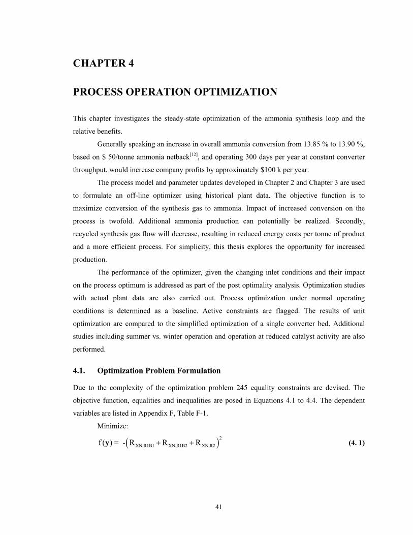
41
CHAPTER 4
PROCESS OPERATION OPTIMIZATION
This chapter investigates the steady-state optimization of the ammonia synthesis loop and the
relative benefits.
Generally speaking an increase in overall ammonia conversion from 13.85 % to 13.90 %,
based on $ 50/tonne ammonia netback[12], and operating 300 days per year at constant converter
throughput, would increase company profits by approximately $100 k per year.
The process model and parameter updates developed in Chapter 2 and Chapter 3 are used
to formulate an off-line optimizer using historical plant data. The objective function is to
maximize conversion of the synthesis gas to ammonia. Impact of increased conversion on the
process is twofold. Additional ammonia production can potentially be realized. Secondly,
recycled synthesis gas flow will decrease, resulting in reduced energy costs per tonne of product
and a more efficient process. For simplicity, this thesis explores the opportunity for increased
production.
The performance of the optimizer, given the changing inlet conditions and their impact
on the process optimum is addressed as part of the post optimality analysis. Optimization studies
with actual plant data are also carried out. Process optimization under normal operating
conditions is determined as a baseline. Active constraints are flagged. The results of unit
optimization are compared to the simplified optimization of a single converter bed. Additional
studies including summer vs. winter operation and operation at reduced catalyst activity are also
performed.
4.1. Optimization Problem Formulation
Due to the complexity of the optimization problem 245 equality constraints are devised. The
objective function, equalities and inequalities are posed in Equations 4.1 to 4.4. The dependent
variables are listed in Appendix F, Table F-1.
Minimize:
( )2XN,R1B1 XN,R1B2 XN,R2f ( ) = - R R R+ +y (4. 1)

42
R1PH,BY
R1PH,SHELL
WHBI,BY
T = T
T
y (4. 2)
Subject to:
jh ( ) = 0 j = 1,2, ..., 245y,u (4. 3)
TG/G,SHELL
R1PH,TUBE
WHBI,TUBE
WHBII,STEAM
HVHV
0 100 = HVHV
≤ ≤
u u (4. 4)
Equality constraints are based on the steady-state versions of the mass and energy
balances developed in Chapter 2. Several intermediate variables are also introduced for
convenience. It is noted that all variables are scaled to solve within a factor of ten and included in
the equation numerator only. Four independent variables, HVG/G,SHELL, HVR1PH,TUBE, HVWHBI,TUBE
and HVWHBII,STEAM are employed in minimizing the objective function. The objective of the
optimizer is to identify feasible controller setpoints within constraints.
4.2. Sensitivity Analysis
An optimal solution gained from a deterministic optimization problem may not by itself be
entirely useful[15] because of uncertainties and possible variations involved in process parameters
or models. Post-optimality analysis is necessary to quantitatively ascertain the sensitivity of the
optimal results to model parameters[15]. In this case, the impact of process disturbances and the
catalyst effectiveness parameter on the calculated optimal converter inlet temperature is explored.
Sensitivities are determined using a first order analysis by perturbation. Methods such as
a Reduced Hessian Strategy[15] exist to evaluate the first order sensitivity of the optimal solution,
with potentially significant computational savings. However, in this case, perturbation of model
formulated in Section 4.1 is used for expediency.
Figure 4-1 looks at the impact of varying inlet pressure to the first reactor bed. The line
traversing the locus of the maxima, often referred to as the “ridge line”, illustrates the optimal
operation of bed one, with changing pressure.

43
Figure 4-1 R1B1 Conversion vs. Inlet Temperature, Varying Pressure5
5
6
7
8
9
325 345 365 385 405 425
Reactor Inlet Temperature, oC
NH 3 C
onve
rsio
n, %
P=19.5P=19.0P=18.5P=18.0P=17.5P=17.0OPT
Figure 4-1 highlights a few key points. The equilibrium favours a higher operating
pressure. An increase of 1 MPa in bed one, impacts ammonia conversion by approximately 0.36
%. As pressure is reduced, the optimum converter inlet temperature increases. Increasing system
pressure by 1 MPa reduces the optimum bed one temperature by approximately 4.6 oC.
The effect of composition on ammonia conversion is often considered in three parts, H/N
ratio, ammonia recycle and inerts. Figures 4-2 and 4-3 illustrate the impact of the H/N ratio and
ammonia recycle on the optimal operation respectively. It is noted that process inerts have the
same directional impact as recycle ammonia.
As can be seen in Figure 4-2 a lower H/N ratio is favoured for ammonia conversion,
which is consistent with nitrogen being the rate-limiting reagent. However the model does not
detect the published optimum H/N ratio of 2.8[41].
5 Based on the following initial process conditions: VIN,SG = 799 k-sm3/hr, P = 18.6 MPa, yNH3 = 2.25 %, yH2/yN2 ratio = 3.2, yINERTS = 15.1 %
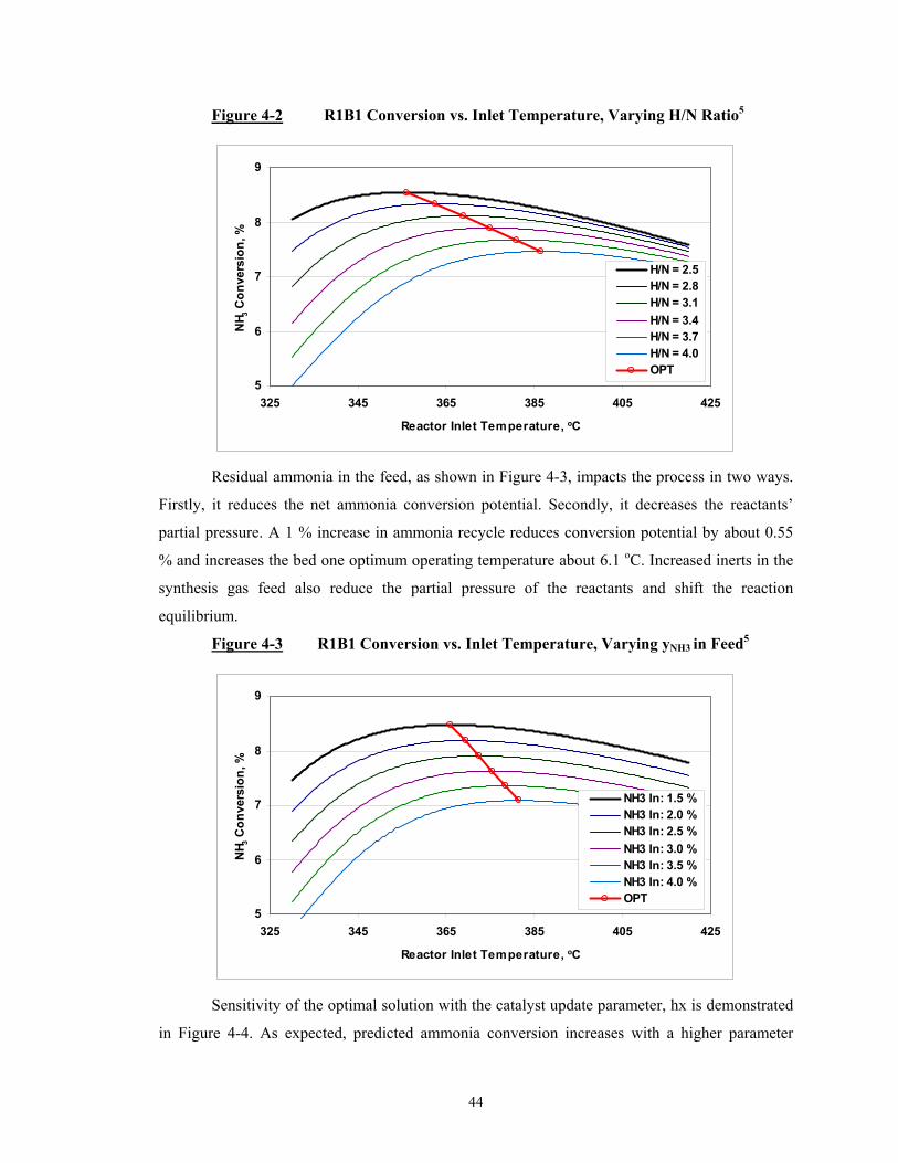
44
Figure 4-2 R1B1 Conversion vs. Inlet Temperature, Varying H/N Ratio5
5
6
7
8
9
325 345 365 385 405 425
Reactor Inlet Temperature, oC
NH 3 C
onve
rsio
n, %
H/N = 2.5H/N = 2.8H/N = 3.1H/N = 3.4H/N = 3.7H/N = 4.0OPT
Residual ammonia in the feed, as shown in Figure 4-3, impacts the process in two ways.
Firstly, it reduces the net ammonia conversion potential. Secondly, it decreases the reactants’
partial pressure. A 1 % increase in ammonia recycle reduces conversion potential by about 0.55
% and increases the bed one optimum operating temperature about 6.1 oC. Increased inerts in the
synthesis gas feed also reduce the partial pressure of the reactants and shift the reaction
equilibrium.
Figure 4-3 R1B1 Conversion vs. Inlet Temperature, Varying yNH3 in Feed5
5
6
7
8
9
325 345 365 385 405 425
Reactor Inlet Temperature, oC
NH 3 C
onve
rsio
n, %
NH3 In: 1.5 %NH3 In: 2.0 %NH3 In: 2.5 %NH3 In: 3.0 %NH3 In: 3.5 %NH3 In: 4.0 %OPT
Sensitivity of the optimal solution with the catalyst update parameter, hx is demonstrated
in Figure 4-4. As expected, predicted ammonia conversion increases with a higher parameter

45
update value. As determined by the slope of the ridge line, a change in the update parameter of
0.05, shifts the optimal setpoint by –1.9 oC.
Figure 4-4 R1B1 Conversion vs. Inlet Temperature, Varying hx Parameter5
5
6
7
8
9
325 345 365 385 405 425
Reactor Inlet Temperature, oC
NH 3 C
onve
rsio
n, %
hx = 1.75hx = 1.70hx = 1.65hx = 1.60hx = 1.55hx = 1.50hx = 1.45OPT
The other interesting point consistent in Figures 4-1 to 4-4 is the insensitivity of the
conversion to changes in temperature near the optimal inlet temperature. Using data from Figures
4-1 to 4-4, the average response of ammonia conversion with temperature around the optimal
inlet temperature is summarized in Table 4-1.
Table 4-1 R1B1 Impact of Temperature Deviation from Optimum
∆T Above Optimum
oC
∆Conversion %
1 -4x10⁻⁴ 5 -0.01
10 -0.0420 -0.13
4.3. Optimization Studies
In this section, the optimal operation is evaluated for different scenarios. Potential benefits are
evaluated where applicable. Scenarios to be considered include normal operation, changing
process conditions and degraded catalyst activity.
4.3.1. Normal Operation
The optimum operating temperatures for February 1999 are solved for each bed. These values are
calculated from the optimization problem formulated in Section 4.1, using historic plant data as

46
the model inputs. Results are presented in Figure 4-5. Realization of these results requires a
suitable control application, discussed further in Chapter 5.
Figure 4-5 Optimal Temperature Profile, Normal Operation–Unit Optimization
325
350
375
400
425
01-Feb 07-Feb 14-Feb 21-Feb 28-Feb
Time
Con
vert
er In
let T
empe
ratu
re, °
C
R1B1 Plant R1B1 ModelR1B2 Plant R1B2 ModelR2 Plant R2 Model
For the month of February, the R1B1 inlet temperature was on average 13 °C above
optimal conditions. Similarly, R1B2 and R2 operated on average 6 °C and 11 °C above the
optimal setpoint. Interestingly, the variance in the optimal setpoints for R1B1, R1B2 and R2, was
only 0.6 °C, 2.3 °C and 0.9 °C. It is noted that the independent variable HVR1PH,TUBE is typically
constrained in the closed position.
Figure 4-6 summarizes the change in ammonia production predicted, equivalent to an
average of +0.52 tonne/hr. Data from this month suggests that a potential of $188 k/year could
have been achieved by running the plant at its optimal operation. These results are tempered by
the results from Chapter 3, which indicated an error of 0.08 tonne/hr between ammonia
production predictions and plant data, Table 3-3.

47
Figure 4-6 Optimal Ammonia Production, Normal Operation–Unit Optimization
75
76
77
78
79
01-Feb 07-Feb 14-Feb 21-Feb 28-Feb
Time
Am
mon
ia P
rodu
ctio
n, to
nne/
hr
Plant DataModel Predictions
The above case study focuses on optimization of the entire synthesis loop. However,
ammonia conversion not achieved in beds one and two can be partially recovered in the third
converter bed. As such a simplified approach, optimization of the last converter is evaluated in
Figures 4-7 and 4-8. Plant operation of TR1B1,IN and TR1B2,IN is assumed to remain constant.
Figure 4-7 R2 Optimal Temperature Profile, Normal Operation–R2 Optimization
385
390
395
400
405
01-Feb 07-Feb 14-Feb 21-Feb 28-Feb
Time
R2
Inle
t Tem
pera
ture
, o C
Plant DataModel Predictions: Opt 3 BedsModel Predictions: Opt 3rd Bed
Figure 4-7 compares the optimal operation of converter inlet temperature for the last
converter with a unit optimization scheme and a simplified optimizer imposed on the last
converter bed. In general, the optimum temperatures for the simplified optimizer are only slightly

48
colder. Performance of the R2 optimizer is summarized in Figure 4-8, which predicts an average
increase in ammonia production of 0.37 tonne/hr.
Figure 4-8 Optimal NH3 Production, Normal Operation-R2 Optimization
75
76
77
78
79
01-Feb 07-Feb 14-Feb 21-Feb 28-Feb
Time
Am
mon
ia P
rodu
ctio
n, to
nne/
hr
Plant DataModel Predictions: Opt 3 BedsModel Predictions: Opt 3rd Bed
In this case, potential returns are approximately $134 k/year. Expressed in other terms,
about 70% of predicted returns can potentially be achieved by optimizing a single loop. The
remaining 30 %, or $ 54 k/year, requires a more complex optimization strategy.
4.3.2. Changing Process Conditions
The above example in section 4.3.1 looked at normal operation of the plant for the month of
February. For comparison of winter and summer operations, winter operation is represented by
the February data set, with data from July representing the summer months. Due to changing
ambient conditions and subsequent process limitations, variation in optimal setpoints is expected.
Most notably, the process operates at a much higher H/N ratio during the summer
months, Figure 4-9. During these months, a process limitation exists in getting sufficient air into
the system. This increases the H/N ratio in the feed gas. Saskferco often reduces feed rates in an
attempt to reduce this saturated control variable. This is shown in Figure 4-10.

49
Figure 4-9 Summer vs. Winter Operation, H/N Ratio
2.4
3.2
4.0
4.8
5.6
1 6 11 16 21 26 31
Day
Synt
hesi
s G
as H
:N R
atio
, mol
/mol
FebruaryJuly
Figure 4-10 Summer vs. Winter Operation, Synthesis Gas
650
700
750
800
850
1 6 11 16 21 26 31
Day
Synt
hesi
s G
as F
eed,
ks-
m3 /h
r
FebruaryJuly
Removal of ammonia and inerts from the recycle gas is a function of the ambient
temperature and process throughput. With the climbing temperatures in the summer, the ammonia
coolers do not run as efficiently, increasing the ammonia recycle into the unit. This is offset with
the reduced rates, which help to improve the inert removal process. The problem with inerts is
further compounded by methane in the fresh feed and a process limitation in the upstream carbon
dioxide removal system. Carbon dioxide, which is a poison to the ammonia catalyst, is converted
to methane in the methanation unit prior to entering the ammonia synthesis loop. The net effect is
reduced inerts in the synthesis gas during the summer months, Figure 4-11.

50
Figure 4-11 Summer vs. Winter Operation, Process Inerts
12
13
14
15
16
17
1 6 11 16 21 26 31
Day
Synt
hesi
s G
as In
erts
, mol
%
FebruaryJuly
The synthesis gas pressure is slightly impacted by changes in the ambient temperature,
Figure 4-12. As noted earlier, the equilibrium favours a higher operating pressure as is shown in
Figure 4-1.
Figure 4-12 Summer vs. Winter Operation, Synthesis Gas Pressure
18.0
18.4
18.8
19.2
19.6
1 6 11 16 21 26 31
Day
Synt
hesi
s G
as P
ress
ure,
MPa
g
FebruaryJuly
Conversion under these changing operations is represented in Figure 4-13.

51
Figure 4-13 Summer vs. Winter Operation, Conversion
12
13
14
15
16
1 6 11 16 21 26 31
Day
Am
mon
ia C
onve
rsio
n, m
ole
%
FebruaryJuly
The process model parameters are updated for July and then substituted into the
optimization model, with the results listed in Figures 4-14 to 4-15. The results indicate slightly
colder optimum temperatures compared to winter operation with increased temperature variation
in the summer months. Resultant production under optimal conditions reveals an average
potential increase of 0.48 tonne/hr.
Figure 4-14 Optimal Temperature Profile, Summer Operation
325
350
375
400
425
01-Jul 06-Jul 11-Jul 16-Jul 21-Jul 26-Jul 31-Jul
Time
Con
vert
er In
let T
empe
ratu
re,
o C
R1B1 Plant R1B1 Model
R1B2 Plant R1B2 ModelR2 Plant R2 Model

52
Figure 4-15 Optimal Ammonia Production, Summer Operation
71
73
75
77
79
1-Jul 6-Jul 11-Jul 16-Jul 21-Jul 26-Jul 31-Jul
Time
Am
mon
ia P
rodu
ctio
n, to
nne/
hr
Plant DataModel Results
Comparison of the July results in Figures 4-14 and 4-15 to February results presented in
Figures 4-5 and 4-6 is summarized in Table 4-2.
Table 4-2 Winter vs. Summer Optimal Operation
TR1B1,IN oC
TR1B2,IN oC
TR2,IN oC
MNH3 tonne/hr
Conv. %
Benefit /year
Winter Range (February)
367-371 399-406 386-390 76.6-78.9 13.2-14.4 $188 k
Summer Range (July)
365-375 395-405 380-386 72.7-77.7 14.4-15.7 $ 173 k
Table 4-2 contrasts the economics of winter and summer operation. The most notable
differences between summer and winter operation are the reduced rates and increased conversion.
As demonstrated in Figures 4-9 to 4-13, more variation occurs in the ammonia synthesis loop
process during the summer months. This increased variation is reflected in the calculated
optimum temperature profile for summer operation. Consolidating summer and winter benefits,
indicates an average potential increase of 0.50 tonne/hour or $180 k/year.
4.3.3. Degraded Catalyst
Iron based ammonia synthesis catalyst is an industry standard, with an expected life of up to 10
years. Deactivation may occur as a result of thermal sintering or poisoning. Poisoning by
oxygenated components, such as water, carbon monoxide and carbon dioxide is largely
reversible, compared to poisons such as sulphur and chlorine that have an irreversible impact on
the catalyst activity[41].

53
This deactivation process effectively reduces the ammonia equilibrium. The reduced
equilibrium has a direct impact on the forward reaction, Equation 4.5, and subsequent ammonia
production.
Pk K+ ∝ (4.5)
By including parameter updates in the optimization problem, the impact of catalyst
deactivation on the optimizer’s performance is reduced. Parameter updates are instituted to fit the
process model to plant data. A shift in the ammonia synthesis equilibrium is compensated for in
Equation 2.20, allowing the optimizer to be sensitive to a change in catalyst activity.
k = hx k_ Kp+ (2.20)
Saskferco was commissioned in 1992. During catalyst reduction, the catalyst in the first
bed was exposed to deactivating conditions and permanent damage[12]. The result is reduced
conversion in the first reactor bed. This increases the potential for ammonia conversion in the
third reactor bed, allowing the optimal inlet temperature of bed three to be pushed slightly below
design conditions. Replacement of the ammonia synthesis catalyst is anticipated in 2006. After
catalyst replacement, it is expected that the optimal inlet temperature for bed three will increase,
based on the improved conversion in bed one.
4.4. Summary of Results
This chapter brings together research done in the previous chapters. Using the process model
developed in Chapter 2, process optimization is explored. The optimizer’s ability to perform in an
accurate and reliable fashion is dependent on both the parameter updates and a controller, yet to
be identified.
The reaction curve, presented in the sensitivity analysis, reveals a band around the
optimum temperature in which conversion indicates a weak relationship to changes in the inlet
temperature. Furthermore, while the model is sensitive to changes in the H/N ratio, it does not
reflect an optimal H/N point as indicated in literature.
The optimization studies identify the opportunity to increase production of the ammonia
plant operation by approximately 0.5 tonne/hr, equivalent to $180 k/year. It is estimated that 70 %
of these results are achievable by optimizing a single converter bed, R2. Optimization results
relative to design and normal operation are compiled in Table 4-3.

54
Table 4-3 Ammonia Conversion: Optimal Performance Comparisons
R1B1 %
R1B2 %
R2 %
Net %
Design6 7.30 3.59 2.74 13.08
Actual 7.93 3.55 2.68 13.57
Optimum – Unit 7.96 3.56 2.73 13.66
Optimum – R2 7.93 3.55 2.74 13.63
Studies around summer and winter seasons indicate notably different operation. Due to
climbing H/N ratios in the summer and increased loop pressure, operations may reduce make-up
synthesis gas. Despite the higher H/N ratio, conversion increases. This suggests that the process
may be diffusion limited at higher feed rates, such that approach to equilibrium is reduced. The
current optimization model assumes a pseudo steady-state and does not account for reactor
residence time. It is noted that residence time in the first bed is approximately three seconds.
Impacts to equilibrium such as reduced catalyst activity are compensated by parameter updates.
This allows optimization calculations to be sensitive to the changing process.
Extension of the optimization model, as an on-line optimizer could be employed given
the appropriate computer resources and process information infrastructure. Frequency of the
optimization calculations and the necessary parameter updates would need to be explored in more
detail.
6 Design numbers are included as a point of interest only. Differences in design and actual conversion in the first bed
are attributed to site improvements in the synthesis feed gas composition.
55
CHAPTER 5
CONTROLLER SYNTHESIS
The first step in designing a control system is to define the control objectives appropriately. These
objectives depend on the goals of the entire plant and of the design of the associated
equipment[27].
The design of the control system must take into consideration the safe and reliable
operation of the plant. For example, adequate level control in WHB I and WHB II is essential.
While level control may not directly impact ammonia production, it is a critical part of the plant’s
operation. The safety control system shutdowns the ammonia plant on either a high or low level
to avoid risk to plant equipment. The level control variable is considered as part of the plant’s
protection system and is designed as a stand-alone regulatory controller.
In general, the control objective of the process considered in this thesis is to control
ammonia production under changing process conditions. To achieve this objective, control of the
ammonia conversion in each reactor bed must be realized. Based on the measured plant variables,
this can be achieved by controlling either the converter inlet temperatures, outlet temperatures or
temperature changes across each reactor bed. For this thesis the inlet temperatures are chosen.
Choosing the reactor beds inlet temperatures has several advantages. They are expected to have
responses closer to linear than the reactor outlet temperatures or the changes in temperature.
PID and multi-variable control (MVC) algorithms are applied to the control problem. In
designing these servo controllers, the variability in the controlled and manipulated variables
needs to be considered. To this end, a maximum overshoot of one tonne/hour of steam production
per one degree Celsius setpoint change is imposed based on feedback from site operations.
Oscillations in steam production inevitably produce oscillations in the steam header pressure.
Without operator intervention, this could trigger a shutdown on level in the waste heat boilers.
Due to the small volume of hold-up in these vessels, this can occur in less than one minute. Note
that the steam header process is not modelled in the process simulation.
The control system should be adaptable to the degrees of freedom available in the
process[27]. The process being considered has more manipulated variables than the number of
control variables. The final controller structure needs to evaluate the effective use of the extra
degrees of freedom.
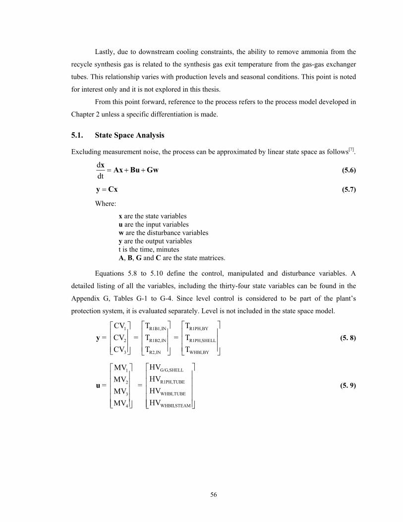
56
Lastly, due to downstream cooling constraints, the ability to remove ammonia from the
recycle synthesis gas is related to the synthesis gas exit temperature from the gas-gas exchanger
tubes. This relationship varies with production levels and seasonal conditions. This point is noted
for interest only and it is not explored in this thesis.
From this point forward, reference to the process refers to the process model developed in
Chapter 2 unless a specific differentiation is made.
5.1. State Space Analysis
Excluding measurement noise, the process can be approximated by linear state space as follows[7].
ddt
= + +x Ax Bu Gw (5.6)
=y Cx (5.7)
Where:
x are the state variables u are the input variables w are the disturbance variables y are the output variables t is the time, minutes A, B, G and C are the state matrices.
Equations 5.8 to 5.10 define the control, manipulated and disturbance variables. A
detailed listing of all the variables, including the thirty-four state variables can be found in the
Appendix G, Tables G-1 to G-4. Since level control is considered to be part of the plant’s
protection system, it is evaluated separately. Level is not included in the state space model.
1 R1B1,IN R1PH,BY
2 R1B2,IN R1PH,SHELL
3 R2,IN WHBI,BY
CV T T = CV = T = T
CV T T
y (5. 8)
G/G,SHELL1
R1PH,TUBE2
WHBI,TUBE3
WHBII,STEAM4
HVMVHVMV
= = HVMVHVMV
u (5. 9)

57
GAS,IN
GAS,IN
NH3,IN
N2,IN
H2,IN
HE,IN
AR,IN
CH4,IN
G/G,SHELL,IN
WHBII,BFW,IN
FPyyy
= yyyTT
w (5. 10)
To determine the local controllability and observability of the system, the state space
matrices are determined by linearizing the process. In developing these matrices, two
simplifications are made. The first simplification is that the derivatives of the compressibility
factor with respect to the state variables are negligible. This is justified based on the weak
relationship between these variables over the range of operation considered. Secondly, when
solving the input gain matrix, B, the bypass flow areas are modelled as a linear function of the
valve opening as defined in Equation 5.11, rather than the more accurate equation given in
Equation 2.54b, which yields a gradient of 0 with input values of 0 % or 100 %.
2Valve
HVAv r 100
π= (5.11)
22 Valve
Valve Valve rHV-50Av (Y-r ) X r asin
50 2π = + +
(2.54b)
Steady-state local input values are substituted into the state space functions. The
evaluated matrices A, B, G and C are listed in Appendix G, Tables G-5 to G-8. From this data,
the controllability of the system is explored. The controllability matrix, P, defined in Equation
5.12 [6], must be full rank to satisfy the criterion for control. 2 33 = P B AB A B A B (5.12)
The rank of P is found to be 3 < 34, indicating a non-controllable system. To find a
controllable sub-space the eighteen reactor compositions are removed from the state variables to
eliminate the near-zero eigenvalues from the A matrix. Additionally, the state derivatives are
rescaled as necessary. The reduced and rescaled state space matrices are listed in Appendix G,
Tables G-9 to G-11. The controllability matrix is then recalculated and found to be a locally
controllable system, with a rank of 16.

58
To allow for state estimation, the observability of the system is evaluated by testing the
rank of the observability matrix O, Equation 5.13. O is also found to be full rank, indicating a
locally observable system.
T TT T T 2 T 15 T = O C A C A C A C (5.13)
5.2. BFW Level Implementation
The level controller, which is required for plant operation, is designed first. The WHB II boiler
feed water (BFW) inlet valve is perturbed +/- 10% to see the impact on the levels in both waste
heat boilers. Refer to Figure 5-1.
Since the WHB level dynamics are naturally integrating, a proportional controller is
implemented to control the level. A gain of one (1 % valve opening/1% level offset) is chosen.
Determination of the gain is based on the need to have fast disturbance rejection, while reducing
the oscillations in the steam system. Comparatively, the level controller implemented on site has a
nonlinear gain ranging from 0.35 to about 1.2, depending on the error and a feedforward term
based on the change in steam production and BFW into the vessel.
The level controller is tested for its ability as a servo controller and as a regulatory
controller.
Controller response to a setpoint change of 10 % is good, reaching steady-state in about
six minutes, with no offset. An overshoot of approximately 2 tonne/hr in steam production
occurs. It is noted that setpoint changes in level are not typical. Refer to Figure 5-2.
In order to test the regulatory performance of the controller, a change of 50 % in the
upstream gas-gas exchanger bypass valve is introduced. This resulted in a 2 tonne/hr drop in
steam production and a steady-state offset of about 1.0 %. Results are shown in Figure 5-3. This
level offset is attributed to the change in the steady-state BFW demand and steam production.
In the last test, the loop is temporarily put into manual and the valve opened 10 % before
placing back into auto control. This test is performed to simulate operator intervention and the
placing of the loop into auto when the process is not at steady-state. The result is again a steady-
state offset. Results can be observed in Figure 5-4.
Based on these tests, it is noted that proportional control applied to the WHB level has
some limitations as a regulatory controller. Alternatively, a proportional integral controller could
be considered. This is rejected, since integral action would introduce more oscillations in the
process and the small offset observed is deemed acceptable.
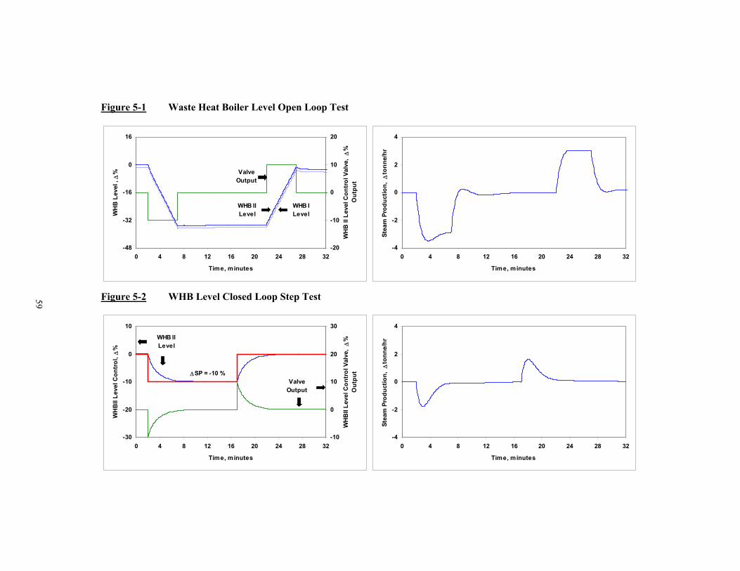
Figure 5-1 Waste Heat Boiler Level Open Loop Test
-48
-32
-16
0
16
0 4 8 12 16 20 24 28 32
Time, minutes
WH
B L
evel
, ∆
%
-20
-10
0
10
20
WH
B II
Lev
el C
ontr
ol V
alve
, ∆
%
Out
put
WHB I Level
WHB II Level
Valve Output
-4
-2
0
2
4
0 4 8 12 16 20 24 28 32
Time, minutes
Stea
m P
rodu
ctio
n, ∆
tonn
e/hr
Figure 5-2 WHB Level Closed Loop Step Test
-30
-20
-10
0
10
0 4 8 12 16 20 24 28 32
Time, minutes
WH
BII
Leve
l Con
trol
, ∆%
-10
0
10
20
30
WH
BII
Leve
l Con
trol
Val
ve,
∆%
O
utpu
t∆SP = -10 %
WHB II Level
Valve Output
-4
-2
0
2
4
0 4 8 12 16 20 24 28 32
Time, minutes
Stea
m P
rodu
ctio
n, ∆
tonn
e/hr
59

Figure 5-3 WHB Level Closed Loop Disturbance Test
-2
-1
0
1
2
0 4 8 12 16 20 24 28 32
Time, minutes
WH
B II
Lev
el, ∆
%
-2
0
2
4
6
WB
H II
Lev
el C
ontr
ol V
alve
, ∆
%
Out
put
WHB II Level
Valve Output
SP
-4
-2
0
2
4
0 4 8 12 16 20 24 28 32
Time, minutes
Stea
m P
rodu
ctio
n, ∆
tonn
e/hr
Figure 5-4 WHB Level Open to Closed Loop Test
-30
-20
-10
0
10
0 4 8 12 16 20 24 28 32
Time, minutes
WH
BII
Leve
l Con
trol
, ∆%
-10
0
10
20
30
WH
BII
Leve
l Con
trol
Val
ve,
∆%
O
utpu
t
∆OP=-10 %
WHB II Level
Valve Output
SP
∆OP=+10 %
-4
-2
0
2
4
0 4 8 12 16 20 24 28 32
Time, minutes
Stea
m P
rodu
ctio
n, ∆
tonn
e/hr
60
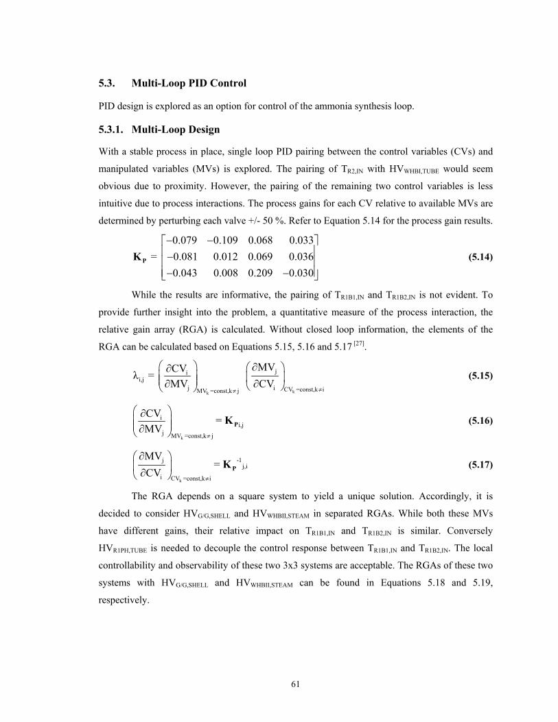
61
5.3. Multi-Loop PID Control
PID design is explored as an option for control of the ammonia synthesis loop.
5.3.1. Multi-Loop Design
With a stable process in place, single loop PID pairing between the control variables (CVs) and
manipulated variables (MVs) is explored. The pairing of TR2,IN with HVWHBI,TUBE would seem
obvious due to proximity. However, the pairing of the remaining two control variables is less
intuitive due to process interactions. The process gains for each CV relative to available MVs are
determined by perturbing each valve +/- 50 %. Refer to Equation 5.14 for the process gain results.
0.079 0.109 0.068 0.033 = 0.081 0.012 0.069 0.036
0.043 0.008 0.209 0.030
− − − − −
PK (5.14)
While the results are informative, the pairing of TR1B1,IN and TR1B2,IN is not evident. To
provide further insight into the problem, a quantitative measure of the process interaction, the
relative gain array (RGA) is calculated. Without closed loop information, the elements of the
RGA can be calculated based on Equations 5.15, 5.16 and 5.17 [27].
kk
jii,j
j i CV =const,k iMV =const,k j
MVCVλ = MV CV
≠≠
∂ ∂ ∂ ∂
(5.15)
k
ii,j
j MV =const,k j
CV = MV
≠
∂ ∂
PK (5.16)
k
-1jj,i
i CV =const,k i
MV=
CV≠
∂ ∂
PK (5.17)
The RGA depends on a square system to yield a unique solution. Accordingly, it is
decided to consider HVG/G,SHELL and HVWHBII,STEAM in separated RGAs. While both these MVs
have different gains, their relative impact on TR1B1,IN and TR1B2,IN is similar. Conversely
HVR1PH,TUBE is needed to decouple the control response between TR1B1,IN and TR1B2,IN. The local
controllability and observability of these two 3x3 systems are acceptable. The RGAs of these two
systems with HVG/G,SHELL and HVWHBII,STEAM can be found in Equations 5.18 and 5.19,
respectively.
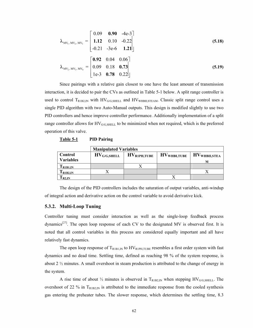
62
1 2 3MV , MV , MV
0.09 -4e-3 = 0.10 -0.22
-0.21 -3e-6
0.901.12
1.21λ (5.18)
2 3 4MV , MV , MV
0.04 0.06 = 0.09 0.18
1e-3 0.22
0.920.73
0.78λ (5.19)
Since pairings with a relative gain closest to one have the least amount of transmission
interaction, it is decided to pair the CVs as outlined in Table 5-1 below. A split range controller is
used to control TR1B2,IN with HVG/G,SHELL and HVWHBII,STEAM. Classic split range control uses a
single PID algorithm with two Auto-Manual outputs. This design is modified slightly to use two
PID controllers and hence improve controller performance. Additionally implementation of a split
range controller allows for HVG/G,SHELL to be minimized when not required, which is the preferred
operation of this valve.
Table 5-1 PID Pairing
Manipulated Variables Control Variables
HVG/G,SHELL HVR1PH,TUBE HVWHBI,TUBE HVWHBII,STEA
M TR1B1,IN X TR1B2,IN X X TR2,IN X The design of the PID controllers includes the saturation of output variables, anti-windup
of integral action and derivative action on the control variable to avoid derivative kick.
5.3.2. Multi-Loop Tuning
Controller tuning must consider interaction as well as the single-loop feedback process
dynamics[27]. The open loop response of each CV to the designated MV is observed first. It is
noted that all control variables in this process are considered equally important and all have
relatively fast dynamics.
The open loop response of TR1B1,IN to HVR1PH,TUBE resembles a first order system with fast
dynamics and no dead time. Settling time, defined as reaching 98 % of the system response, is
about 2 ½ minutes. A small overshoot in steam production is attributed to the change of energy in
the system.
A rise time of about ½ minutes is observed in TR1B2,IN when stepping HVG/G,SHELL. The
overshoot of 22 % in TR1B2,IN is attributed to the immediate response from the cooled synthesis
gas entering the preheater tubes. The slower response, which determines the settling time, 8.3

63
minutes, is based on the synthesis gas recycling back through the shell side of the preheater.
Again, steam production is impacted, with negligible overshoot.
The opening of HVWHBII,STEAM results in a slight inverse response in TR1B2,IN.
Approximating this behaviour by a first order system yields about a 4 minute deadtime. When
HVWHBII,STEAM is closed, a dead time of approximately 2 minutes is noted, without an inverse
response. The dynamics attributed to this MV are significantly slower than the processes
observed earlier, with a settling time of 22 ½ minutes. This is a result of the interaction with the
steam system and the change in heat distribution between WHB I and WHB II. While steady-state
steam production remained relatively constant, opening this MV 50 % results in a -10.2 tonne/hr
overshoot in steam production. Comparatively, closing the valve 50 % causes a 12.5 tonne/hr
overshoot. As HVWHBII,STEAM has the largest impact on steam oscillations, it is necessary to detune
this control loop to honour the restriction of a maximum overshoot of one tonne/hour of steam
production per one degrees Celsius change. Due to the hysteresis observed, both a positive and
negative unit step test are required to ensure the control objectives are satisfied.
The impact of HVWHBI,TUBE on TR2,IN is almost immediate. TR2,IN is the mix temperature of
the cooled synthesis gas exiting the WHB I tubes and the warmer synthesis gas from R1B2,
bypassing WHB I. Closing the WHB I bypass valve immediately decreases the bypass flow and
the subsequent mix temperature. The response is tempered as the synthesis gas exiting the WHB I
tubes warms slightly as more flow is diverted to this exchanger. The result is a rise time of less
than one second and a settling time of approximately 8 minutes. An overshoot in steam
production is observed.
Based on this open loop information, determined by perturbing the process model, the
controller gains and integral times are evaluated. The controller gains are then detuned to achieve
the desired process response. In general, to reach the desired setpoint the controller gains do not
change significantly, despite process interactions. However, when the other control objectives are
imposed, such as minimizing variation in the manipulated variables and steam production, the
control problem becomes more difficult, requiring significant detuning. The final controller
tuning values are available in Table 5-2. Open loop results are available graphically in Appendix
G, Figures G-1 to G-5.
Table 5-2 PID Tuning
TR1B1,IN TR1B2,IN (HVG/G,SHELL)
TR1B2,IN (HVWHBII,STEAM)
TR2,IN
KC ( )o%
C -6.96 -9.26 1.20 3.59
τI (minutes) 0.62 0.20 2.00 0.05τD (minutes) 0 0 1.40 0
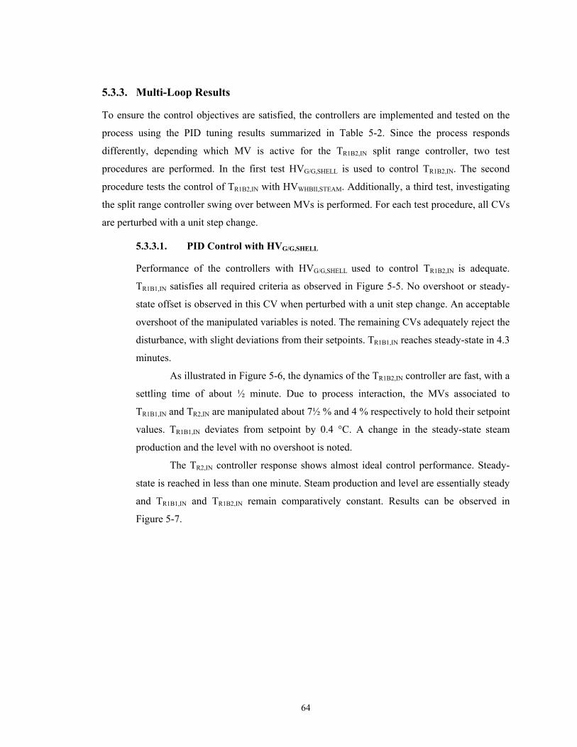
64
5.3.3. Multi-Loop Results
To ensure the control objectives are satisfied, the controllers are implemented and tested on the
process using the PID tuning results summarized in Table 5-2. Since the process responds
differently, depending which MV is active for the TR1B2,IN split range controller, two test
procedures are performed. In the first test HVG/G,SHELL is used to control TR1B2,IN. The second
procedure tests the control of TR1B2,IN with HVWHBII,STEAM. Additionally, a third test, investigating
the split range controller swing over between MVs is performed. For each test procedure, all CVs
are perturbed with a unit step change.
5.3.3.1. PID Control with HVG/G,SHELL
Performance of the controllers with HVG/G,SHELL used to control TR1B2,IN is adequate.
TR1B1,IN satisfies all required criteria as observed in Figure 5-5. No overshoot or steady-
state offset is observed in this CV when perturbed with a unit step change. An acceptable
overshoot of the manipulated variables is noted. The remaining CVs adequately reject the
disturbance, with slight deviations from their setpoints. TR1B1,IN reaches steady-state in 4.3
minutes.
As illustrated in Figure 5-6, the dynamics of the TR1B2,IN controller are fast, with a
settling time of about ½ minute. Due to process interaction, the MVs associated to
TR1B1,IN and TR2,IN are manipulated about 7½ % and 4 % respectively to hold their setpoint
values. TR1B1,IN deviates from setpoint by 0.4 °C. A change in the steady-state steam
production and the level with no overshoot is noted.
The TR2,IN controller response shows almost ideal control performance. Steady-
state is reached in less than one minute. Steam production and level are essentially steady
and TR1B1,IN and TR1B2,IN remain comparatively constant. Results can be observed in
Figure 5-7.
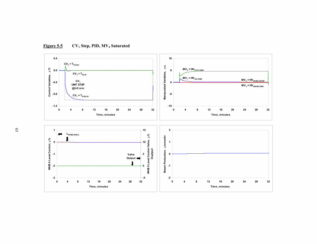
Figure 5-5 CV1 Step, PID, MV4 Saturated
-1.2
-0.8
-0.4
0.0
0.4
0 4 8 12 16 20 24 28 32
Time, minutes
Con
trol
Var
iabl
es,
∆o C
CV2 = TR1B,IN
CV3 = TR2,IN
CV1 = TR1B2,IN
CV1 UNIT STEP @t=2 min
-16
-8
0
8
16
0 4 8 12 16 20 24 28 32
Time, minutes
Man
ipul
ated
Var
iabl
es,
∆%
MV2 = HVR1PH,TUBE
MV3 = HVRWHBI,TUBE
MV1 = HVG/G,TUBE MV4 = HVWHBII,STEAM
-3
-2
-1
0
1
0 4 8 12 16 20 24 28 32
Time, minutes
WH
B II
Lev
el C
ontr
ol, ∆
%
-5
0
5
10
15
WH
B II
Lev
el C
ontr
ol V
alve
, ∆
%
Oup
tput
LWHBII,SHELL
Valve Output
-2
-1
0
1
2
0 4 8 12 16 20 24 28 32
Time, minutes
Stea
m P
rodu
ctio
n, ∆
tonn
e/hr
65
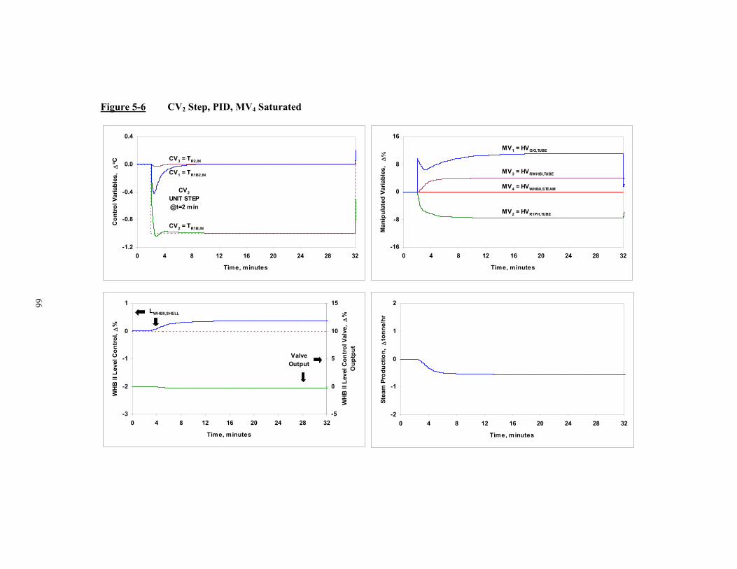
Figure 5-6 CV2 Step, PID, MV4 Saturated
-1.2
-0.8
-0.4
0.0
0.4
0 4 8 12 16 20 24 28 32
Time, minutes
Con
trol
Var
iabl
es,
∆o C
CV2 = TR1B,IN
CV3 = TR2,IN
CV1 = TR1B2,IN
CV2 UNIT STEP @t=2 min
-16
-8
0
8
16
0 4 8 12 16 20 24 28 32
Time, minutes
Man
ipul
ated
Var
iabl
es,
∆%
MV2 = HVR1PH,TUBE
MV3 = HVRWHBI,TUBE
MV1 = HVG/G,TUBE
MV4 = HVWHBII,STEAM
-3
-2
-1
0
1
0 4 8 12 16 20 24 28 32
Time, minutes
WH
B II
Lev
el C
ontr
ol, ∆
%
-5
0
5
10
15
WH
B II
Lev
el C
ontr
ol V
alve
, ∆
%
Oup
tput
LWHBII,SHELL
Valve Output
-2
-1
0
1
2
0 4 8 12 16 20 24 28 32
Time, minutes
Stea
m P
rodu
ctio
n, ∆
tonn
e/hr
66

Figure 5-7 CV3 Step, PID, MV4 Saturated
-1.2
-0.8
-0.4
0.0
0.4
0 4 8 12 16 20 24 28 32
Time, minutes
Con
trol
Var
iabl
es,
∆o C CV2 = TR1B,IN
CV3 = TR2,IN
CV1 = TR1B2,IN
CV3 UNIT STEP @t=2 min
-16
-8
0
8
16
0 4 8 12 16 20 24 28 32
Time, minutes
Man
ipul
ated
Var
iabl
es,
∆%
MV2 = HVR1PH,TUBE
MV3 = HVRWHBI,TUBE
MV1 = HVG/G,TUBE
MV4 = HVWHBII,STEAM
-3
-2
-1
0
1
0 4 8 12 16 20 24 28 32
Time, minutes
WH
B II
Lev
el C
ontr
ol, ∆
%
-5
0
5
10
15
WH
B II
Lev
el C
ontr
ol V
alve
, ∆
%
Oup
tputLWHBII,SHELL Valve
Output
-2
-1
0
1
2
0 4 8 12 16 20 24 28 32
Time, minutes
Stea
m P
rodu
ctio
n, ∆
tonn
e/hr
67

68
5.3.3.2. PID Control with HVWHBII,STEAM
Results in this case met the design criteria, but the overall performance is diminished.
Again the TR1B1,IN controller satisfies all required criteria. The settling time of 3.3
minutes is about 25 % less than the first case. This is a consequence of the relatively slow
control action with HVWHBII,STEAM and subsequent interaction with TR1B1,IN. Steam
production and level are affected slightly due to the disturbance on TR1B2,IN. Figure 5-8
demonstrates the TR1B1,IN control performance.
Figure 5-9 illustrates the response of the TR1B2,IN controller with HVWHBII,STEAM.
The predominant characteristic of this controller is the settling time of 107 minutes.
Detuning of the HVWHBII,STEAM/TR1B2,IN controller is done to meet constraints in the steam
production system. Steam overshoot in this case is 1 tonne/hr per 1°C setpoint change,
equal to the constraint imposed. This detuned controller, with respect to the interaction
between other CVs, imposes a smaller disturbance compared to HVG/G,SHELL. This allows
TR1B1,IN and TR2,IN to return to steady-state more rapidly than when TR1B2,IN is controlled
with HVG/G,SHELL. However, the controllers’ ability to reject disturbances degrades.
The TR2,IN control performance with HVWHBII,STEAM controlling TR1B2,IN is notably
different than the TR2,IN step response with HVG/G,SHELL controlling TR1B2,IN. While TR2,IN
reaches steady-state in less than one minute, increased valve action is noted. Also in this
case, both the TR1B1,IN and TR1B2,IN outputs are manipulated to maintain their setpoints.
TR1B2,IN deviates from setpoint by 0.4°C. It requires about 110 minutes to return to steady-
state. An oscillation in the steam system, of 0.97 tonne/hr is within design criteria. These
observations are based on Figure 5-10.

Figure 5-8 CV1 Step, PID, MV1 Saturated
-0.4
0.0
0.4
0.8
1.2
0 20 40 60 80 100 120
Time, minutes
Con
trol
Var
iabl
es,
∆o C
CV3 = TR2,IN
CV1 = TR1B1,IN
CV2 = TR1B2,IN
CV1 UNIT STEP @t=2 min
-16
-8
0
8
16
0 20 40 60 80 100 120
Time, minutes
Man
ipul
ated
Var
iabl
es,
∆%
MV2 = HVR1PH,TUBE
MV3 = HVWHBI,TUBE
MV4 = HVWHBII,STEAM
MV1 = HVG/G,SHELL
-3
-2
-1
0
1
0 20 40 60 80 100 120
Time, minutes
WH
B II
Lev
el C
ontr
ol, ∆
%
-5
0
5
10
15
WH
B II
Lev
el C
ontr
ol V
alve
, ∆
%
Oup
tput
LWHBII,SHELL
Valve Output
-2
-1
0
1
2
0 20 40 60 80 100 120
Time, minutes
Stea
m P
rodu
ctio
n, ∆
tonn
e/hr
69
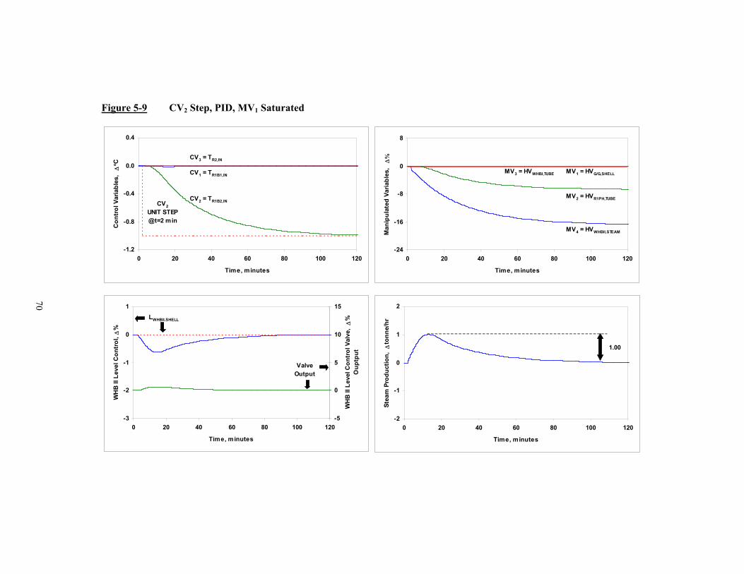
Figure 5-9 CV2 Step, PID, MV1 Saturated
-1.2
-0.8
-0.4
0.0
0.4
0 20 40 60 80 100 120
Time, minutes
Con
trol
Var
iabl
es,
∆o C
CV3 = TR2,IN
CV1 = TR1B1,IN
CV2 = TR1B2,INCV2 UNIT STEP @t=2 min
-24
-16
-8
0
8
0 20 40 60 80 100 120
Time, minutes
Man
ipul
ated
Var
iabl
es,
∆%
MV2 = HVR1PH,TUBE
MV3 = HVWHBI,TUBE
MV4 = HVWHBII,STEAM
MV1 = HVG/G,SHELL
-3
-2
-1
0
1
0 20 40 60 80 100 120
Time, minutes
WH
B II
Lev
el C
ontr
ol, ∆
%
-5
0
5
10
15
WH
B II
Lev
el C
ontr
ol V
alve
, ∆
%
Oup
tput
LWHBII,SHELL
Valve Output
-2
-1
0
1
2
0 20 40 60 80 100 120
Time, minutes
Stea
m P
rodu
ctio
n, ∆
tonn
e/hr
1.00
70

Figure 5-10 CV3 Step, PID, MV1 Saturated
-1.2
-0.8
-0.4
0.0
0.4
0 20 40 60 80 100 120
Time, minutes
Con
trol
Var
iabl
es,
∆o C
CV3 = TR2,IN
CV1 = TR1B1,IN
CV2 = TR1B2,IN
CV3 UNIT STEP @t=2 min
-16
-8
0
8
16
0 20 40 60 80 100 120
Time, minutes
Man
ipul
ated
Var
iabl
es,
∆%
MV2 = HVR1PH,TUBE MV3 = HVWHBI,TUBE
MV4 = HVWHBII,STEAM
MV1 = HVG/G,SHELL
-3
-2
-1
0
1
0 20 40 60 80 100 120
Time, minutes
WH
B II
Lev
el C
ontr
ol, ∆
%
-5
0
5
10
15
WH
B II
Lev
el C
ontr
ol V
alve
, ∆
%
Oup
tput
LWHBII,SHELL
Valve Output
-2
-1
0
1
2
0 20 40 60 80 100 120
Time, minutes
Stea
m P
rodu
ctio
n, ∆
tonn
e/hr
0.93
71

72
5.3.3.3. TR1B2,IN Split Range PID Control
To demonstrate the functionality of the split range controller a setpoint change of 5 °C is
performed, as shown in Figure 5-11. While controller setpoints are achieved, the
transition from HVWHBII,STEAM to HVG/G,SHELL introduces additional disturbances in the
process, specifically in the steam system. A change in steam production of 6.4 tonne/hr
introduces the possibility of oscillations in the steam system. However, the overshoot of
about 1.03 tonne/hr steam per 1 °C setpoint change is considered sufficiently close to the
criteria set. The transition from HVG/G,SHELL to HVWHBII,STEAM, Figure 5-12, produces a
smoother response.

Figure 5-11 CV2 Step Down, Split Range Controller
-6
-4
-2
0
2
0 10 20 30 40 50 60
Time, minutes
Con
trol
Var
iabl
es,
∆o C
CV3 = TR2,IN
CV1 = TR1B1,IN
CV2 = TR1B2,IN
CV2 -5 oC STEP @t=2 min
-60
-30
0
30
60
0 10 20 30 40 50 60
Time, minutes
Man
ipul
ated
Var
iabl
es,
∆%
MV2 = HVR1PH,TUBE
MV3 = HVWHBI,TUBE
MV4 = HVWHBII,STEAM
MV1 = HVG/G,SHELL
@t=25 min- MV4 fully closed- MV1 opening
-6
-4
-2
0
2
0 10 20 30 40 50 60
Time, minutes
WH
B II
Lev
el C
ontr
ol, ∆
%
-2
2
6
10
14
WH
B II
Lev
el C
ontr
ol V
alve
, ∆
%
Oup
tput
LWHBII,SHELL
Valve Output
-2
0
2
4
6
0 10 20 30 40 50 60
Time, minutes
Stea
m P
rodu
ctio
n, ∆
tonn
e/hr
6.4
5.1
73

Figure 5-12 CV2 Step Up, Split Range Controller - CV Response
-6
-4
-2
0
2
60 80 100 120 140 160 180
Time, minutes
Con
trol
Var
iabl
es,
∆o C
CV3 = TR2,IN
CV1 = TR1B1,IN
CV2 = TR1B2,IN
CV2 +5 oC STEP @t=62 min
-60
-30
0
30
60
60 80 100 120 140 160 180
Time, minutes
Man
ipul
ated
Var
iabl
es,
∆%
MV2 = HVR1PH,TUBE
MV3 = HVWHBI,TUBE
MV4 = HVWHBII,STEAM
MV1 = HVG/G,SHELL
@t=63 min- MV1 fully closed- MV4 opening
-6
-4
-2
0
2
60 80 100 120 140 160 180
Time, minutes
WH
B II
Lev
el C
ontr
ol, ∆
%
-2
2
6
10
14
WH
B II
Lev
el C
ontr
ol V
alve
, ∆
%
Oup
tput
LWHBII,SHELL
Valve Output
-2
0
2
4
6
60 80 100 120 140 160 180
Time, minutes
Stea
m P
rodu
ctio
n,
tonn
e/hr
1.76
74

75
5.4. Linear Multi-Variable Control
While several modifications have been made to the conventional PID form, such as gain-
scheduling, nonlinear gains, output characterization, split range controllers, etc., it remains best
suited for single input, single output (SISO) systems over a near-linear process. Comparatively,
multivariable control (MVC) considers the process as a complete system, allowing a wider range
of applicability. While considerable time may be required for implementation, potential returns
on the implementation of a multi-input, multi-output (MIMO) system make it an attractive control
option relative to PID.
Initially multivariable predictive control (MPC) was considered for MVC control studies.
MPC is an industry standard for MVC applications and tools are readily available. However,
implementation of this controller type on similar ammonia facilities has successfully been
demonstrated[19],[22]. Based on this information, it is decided to explore the design and
implementation of a linear quadratic regulator (LQR). Although commercial engineering tools are
not as available compared to MPC, effort to design the LQR is not considered prohibitive.
Further, an LQR algorithm can have a smaller on-line computational cost than MPC.
- MVC Design
The LQR control problem is an optimal controller that attempts to minimize a user supplied
quadratic performance index or cost function (J)[8]. The cost function, Equation 5.20 is designed
to drive the state or part of the state of the system to zero without using excessive input energy[5].
The weighting matrices for the control variables and process inputs, Q and R, are tuned by trial
and error by the controls engineer to achieve the desired control performance. Knowledge of the
process and relative importance of the control variables is used to determine reasonable initial
values of the weighting matrix. The performance index is posed to look at the change in valve
movement for each controller step made[9]. This is done to eliminate steady-state offset from
setpoint and is achieved by discretizing the LQR controller with a zero order hold, and a sample
period of one second.
( )T T
0J = + dt
∞∆ ∆∫ x Q x u R u (5.20)
The state feedback control law that results from the solution of the LQR problem has the
following form, Equation 5.21. u* is the optimal controller input and KC is the controller gain
matrix. * = - Cu K x (5.21)

76
Solution of the infinite time LQR problem uses the well known algebraic Riccati
equation[5] and yields Equation 5.22. S is the Riccati matrix. T -1= CK S B R (5.22)
Since not all of the states are available, a state observer is required to implement this
controller. Accordingly, a Kalman Filter is used to estimate the state variables from measured and
input variables, y and u. Refer to Equations 5.23 and 5.24[21].
( )ˆd ˆ ˆ - dt
= + +x A x B u L y C x (5.23)
ˆ ˆ =y C x (5.24)
The estimator gain, L, is used to drive the error of the estimated states to zero based on a
weighting matrix and the Riccati matrix[21]. The weighting matrix is equal to the inverse of the
measurement covariance matrix, as identified in Equations 3.15 and 3.16. Measurement error is
based on the error between the process model and the Kalman Filter estimate. T T = L W C S (5.25)
ˆ ˆ = - = - e y y y Cx (5.26)
Combining the state estimator with the optimal control vector yields the output feedback
linear quadratic Gaussian regulator, LQGR[21], Equations 5.27 and 5.28. LQGR is implemented as
a discrete controller, using a zero order hold and a sample period of one second.
d + dt
=x A x B y (5.27)
+ =u C x D y (5.28)
5.4.1. MVC Tuning
Tuning of the LQR controller is based on a locally linearized model of the process. Consistent
with industry practices, the controller is tested and tuned on this same linearized model, prior to
implementation[4]. This allows for immediate feedback without disrupting operations and in some
cases is used for operator training.
As a starting point, noting that all CVs are equally important, the identity matrix is used
for the weighting matrices Q and R. Subsequent tuning of Q and R is achieved iteratively. The
resulting control action and performance yields positive results for each CV. Noting that the PID
controller is able to effectively handle the saturation of HVG/G,SHELL, the performance of the LQR
controller under these conditions is also considered. With HVG/G,SHELL dropped from the control
problem the controller is unable to converge to a steady operating point, triggering the process to

77
become unstable. Iterative tuning of Q and R proves to be inadequate to identify a suitable
controller.
A new term, N, designed to promote loop pairings between controller inputs and outputs
is introduced into the performance index[21], Equation 5.29. With this information and knowledge
of the loop pairing identified in Table 5-1 using the RGA, N is used to promote control of TR1B2,IN
with HVWHBII,STEAM.
( )T T
0J = + + 2 dt
∞∆ ∆ ∆∫ Tx Q x u R u x N u (5.29)
Using this modified controller with HVG/G,SHELL saturated, TR1B2,IN has a settling time of
approximately 60 minutes for the linearized process model. This is a significant improvement
over the PID control observed in section 4.2. An overshoot in steam production of 0.9 tonne per
hour is noted. Validation of these results with the process is explored in Section 5.4.2, with the
tuning constants presented in Equation 5.30.
1 0 0 01 0 0 0 0 0 0
0 1 0 0 2= 2 0 1 0 = = 0 0 0 10 0 1 0 100
0 0 1 0 0 0 00 0 0 1
Q R N (5.30)
5.4.2. MVC Results
The LQR controller is then implemented on the process. The process response to the LQR with
MV1 saturated is tested first. The process remains stable with a settling time of 60 minutes,
similar to the linear model results. However, steady-state offset in the control variables is
observed as well as an overshoot in steam production of 2.3 tonne/hr. Results are presented in
Figure 5-13. This behaviour is notably different than the response observed in the linearized
process model. The controller is then re-tuned to meet specifications.
1 0 0 01 0 0 0 0 0 0
0 1 0 0 1.065= 2 0 1 0 = = 0 0 0 10 0 1 0 100
0 0 1 0 0 0 00 0 0 1
Q R N (5.31)
With the revised controller tuning constants, Equation 5.31, a stable process response for
all CVs is achieved within controller specifications. The process control response for a step in
each CV with HVG/G,TUBE saturated can be found in Figures 5-14 to 5-16. Comparatively graphical
results with HVWHBII,STEAM are included in Figures 5-17 to 5-19. Significant improvement in
settling times compared to PID control results are marked.

Figure 5-13 CV2 Step, Modified LQR, MV1 Saturated
-0.5
0.0
0.5
1.0
1.5
0 20 40 60 80 100 120
Time, minutes
Con
trol
Var
iabl
es,
∆o C
CV2 = TR1B2,IN
CV1 = TR1B1,IN
CV3 = TR2,IN
CV2 UNIT STEP @t=2 min.
-10
0
10
20
30
0 20 40 60 80 100 120
Time, minutes
Man
ipul
ated
Var
iabl
es,
∆%
MV1 = HVG/G.SHELL
MV2 = HVR1PH,TUBE
MV3 = HVWHBI,TUBE
MV4 = HVWHBII,STEAM
-4
-2
0
2
4
0 20 40 60 80 100 120
Time, minutes
WH
B II
Lev
el C
ontr
ol ∆
%
-2
0
2
4
6
WH
B II
Lev
el C
ontr
ol V
alve
, ∆
%
Out
put
LWHBII,SHELL
Valve Output
-2
-1
0
1
2
0 20 40 60 80 100 120
Time, minutes
Stea
m P
rodu
ctio
n, ∆
tonn
e/hr
2.3
78
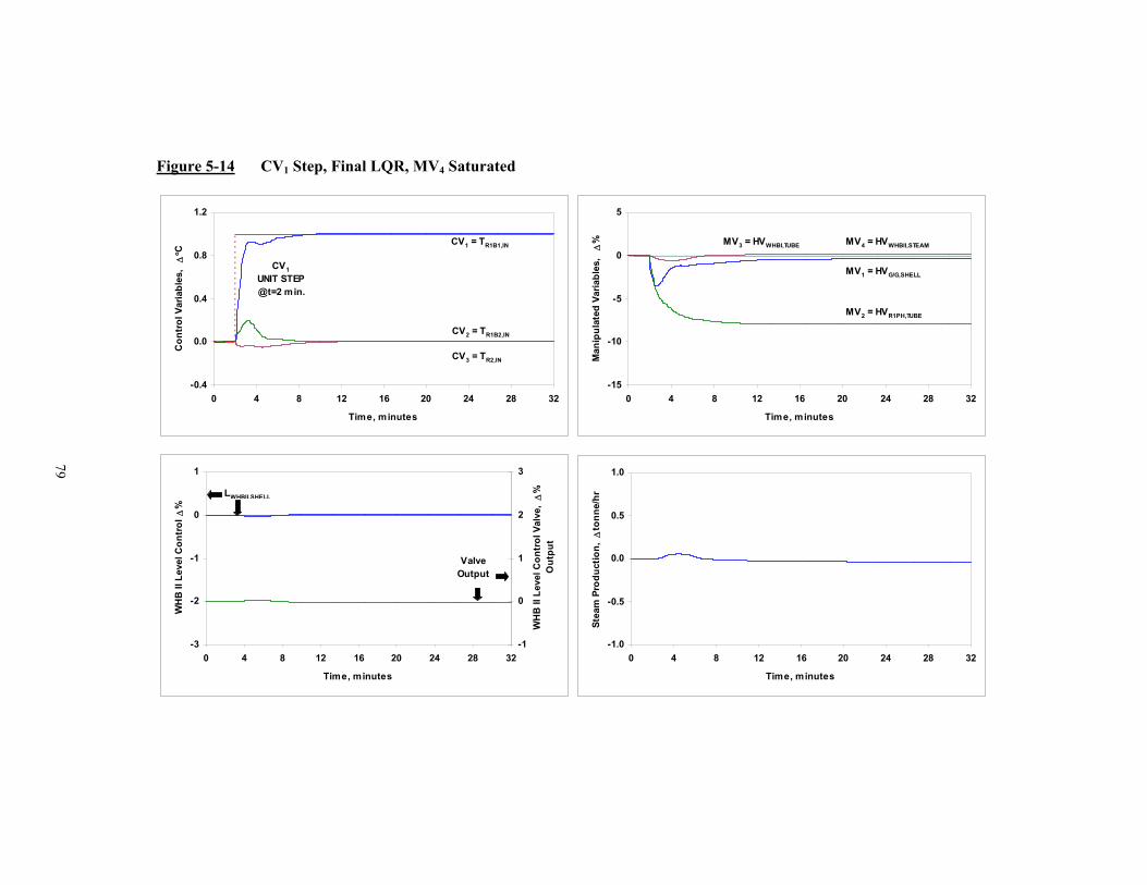
Figure 5-14 CV1 Step, Final LQR, MV4 Saturated
-0.4
0.0
0.4
0.8
1.2
0 4 8 12 16 20 24 28 32
Time, minutes
Con
trol
Var
iabl
es,
∆o C
CV1 = TR1B1,IN
CV2 = TR1B2,IN
CV3 = TR2,IN
CV1 UNIT STEP @t=2 min.
-15
-10
-5
0
5
0 4 8 12 16 20 24 28 32
Time, minutes
Man
ipul
ated
Var
iabl
es,
∆%
MV1 = HVG/G,SHELL
MV2 = HVR1PH,TUBE
MV3 = HVWHBI,TUBE MV4 = HVWHBII,STEAM
-3
-2
-1
0
1
0 4 8 12 16 20 24 28 32
Time, minutes
WH
B II
Lev
el C
ontr
ol ∆
%
-1
0
1
2
3
WH
B II
Lev
el C
ontr
ol V
alve
, ∆
%
Out
put
LWHBII,SHELL
Valve Output
-1.0
-0.5
0.0
0.5
1.0
0 4 8 12 16 20 24 28 32
Time, minutes
Stea
m P
rodu
ctio
n, ∆
tonn
e/hr
79
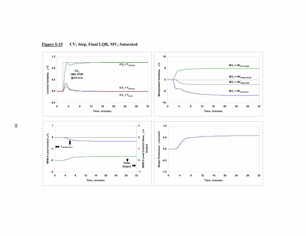
Figure 5-15 CV2 Step, Final LQR, MV4 Saturated
-0.4
0.0
0.4
0.8
1.2
0 4 8 12 16 20 24 28 32
Time, minutes
Con
trol
Var
iabl
es,
∆o C
CV2 = TR1B2,IN
CV1 = TR1B1,IN
CV3 = TR2,IN
CV2 UNIT STEP @t=2 min.
-16
-8
0
8
16
0 4 8 12 16 20 24 28 32
Time, minutes
Man
ipul
ated
Var
iabl
es,
∆%
MV1 = HVG/G.SHELL
MV2 = HVR1PH,TUBE
MV3 = HVWHBI,TUBE
MV4 = HVWHBII,STEAM
-3
-2
-1
0
1
0 4 8 12 16 20 24 28 32
Time, minutes
WH
B II
Lev
el C
ontr
ol ∆
%
-1
0
1
2
3
WH
B II
Lev
el C
ontr
ol V
alve
, ∆
%
Out
put
LWHBII,SHELL
Valve Output
-1.0
-0.5
0.0
0.5
1.0
0 4 8 12 16 20 24 28 32
Time, minutes
Stea
m P
rodu
ctio
n, ∆
tonn
e/hr
80

Figure 5-16 CV3 Step, Final LQR, MV4 Saturated
-0.4
0.0
0.4
0.8
1.2
0 4 8 12 16 20 24 28 32
Time, minutes
Con
trol
Var
iabl
es,
∆o C
CV1 = TR1B1,IN
CV2 = TR1B2,IN
CV3 = TR2,IN
CV3 UNIT STEP @t=2 min.
-4
0
4
8
12
0 4 8 12 16 20 24 28 32
Time, minutes
Man
ipul
ated
Var
iabl
es,
∆%
MV1 = HVG/G.SHELL
MV2 = HVR1PH,TUBE
MV3 = HVWHBI,TUBE
MV4 = HVWHBII,STEAM
-3
-2
-1
0
1
0 4 8 12 16 20 24 28 32
Time, minutes
WH
B II
Lev
el C
ontr
ol ∆
%
-1
0
1
2
3
WH
B II
Lev
el C
ontr
ol V
alve
, D%
O
utpu
t
LWHBII,SHELL
Valve Output
-1.0
-0.5
0.0
0.5
1.0
0 4 8 12 16 20 24 28 32
Time, minutes
Stea
m P
rodu
ctio
n, ∆
tonn
e/hr
81
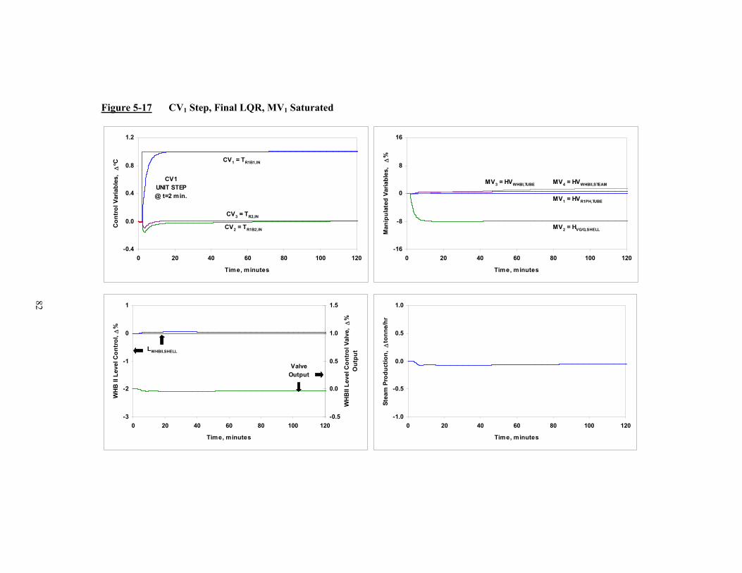
Figure 5-17 CV1 Step, Final LQR, MV1 Saturated
-0.4
0.0
0.4
0.8
1.2
0 20 40 60 80 100 120
Time, minutes
Con
trol
Var
iabl
es,
∆o C
CV2 = TR1B2,IN
CV1 = TR1B1,IN
CV3 = TR2,IN
CV1 UNIT STEP @ t=2 min.
-16
-8
0
8
16
0 20 40 60 80 100 120
Time, minutes
Man
ipul
ated
Var
iabl
es,
∆%
MV2 = HVG/G,SHELL
MV4 = HVWHBII,STEAM
MV1 = HVR1PH,TUBE
MV3 = HVWHBI,TUBE
-3
-2
-1
0
1
0 20 40 60 80 100 120
Time, minutes
WH
B II
Lev
el C
ontr
ol, ∆
%
-0.5
0.0
0.5
1.0
1.5
WH
BII
Leve
l Con
trol
Val
ve,
∆%
O
utpu
tLWHBII,SHELL
Valve Output
-1.0
-0.5
0.0
0.5
1.0
0 20 40 60 80 100 120
Time, minutes
Stea
m P
rodu
ctio
n, ∆
tonn
e/hr
82
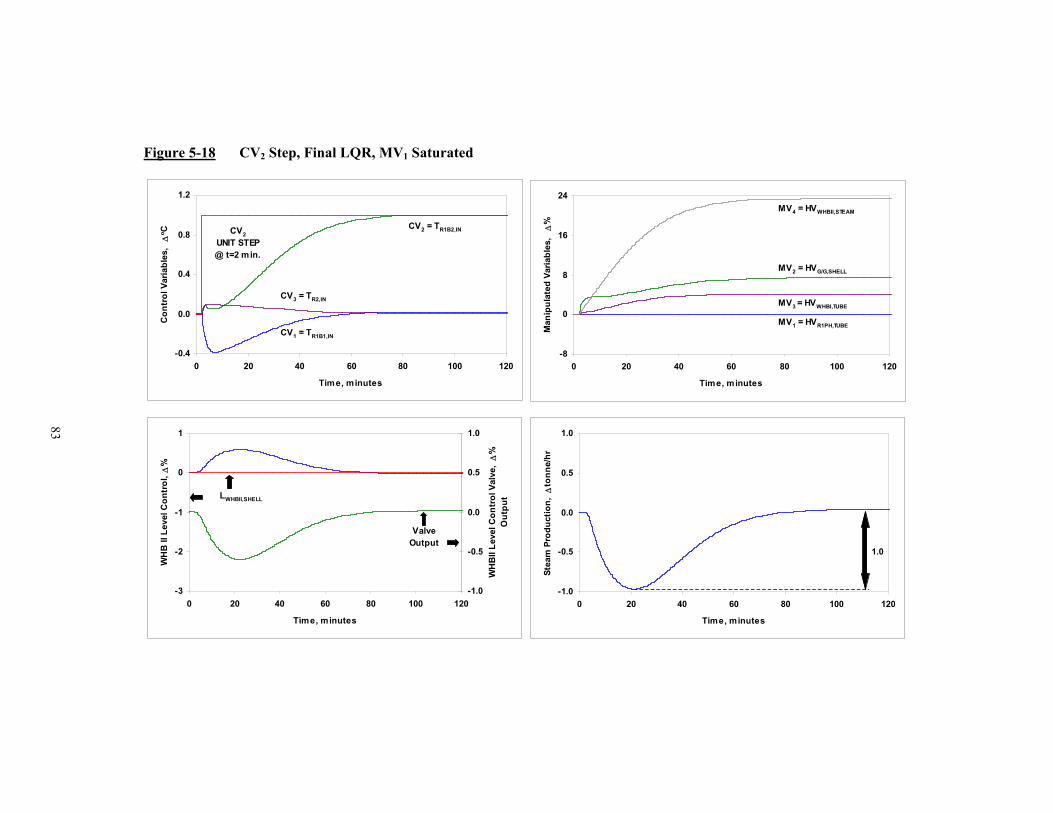
Figure 5-18 CV2 Step, Final LQR, MV1 Saturated
-0.4
0.0
0.4
0.8
1.2
0 20 40 60 80 100 120
Time, minutes
Con
trol
Var
iabl
es,
∆o C
CV2 = TR1B2,IN
CV1 = TR1B1,IN
CV3 = TR2,IN
CV2 UNIT STEP @ t=2 min.
-8
0
8
16
24
0 20 40 60 80 100 120
Time, minutes
Man
ipul
ated
Var
iabl
es,
∆%
MV2 = HVG/G,SHELL
MV4 = HVWHBII,STEAM
MV1 = HVR1PH,TUBE
MV3 = HVWHBI,TUBE
-3
-2
-1
0
1
0 20 40 60 80 100 120
Time, minutes
WH
B II
Lev
el C
ontr
ol, ∆
%
-1.0
-0.5
0.0
0.5
1.0
WH
BII
Leve
l Con
trol
Val
ve,
∆%
O
utpu
tLWHBII,SHELL
Valve Output
-1.0
-0.5
0.0
0.5
1.0
0 20 40 60 80 100 120
Time, minutes
Stea
m P
rodu
ctio
n, ∆
tonn
e/hr
1.0
83
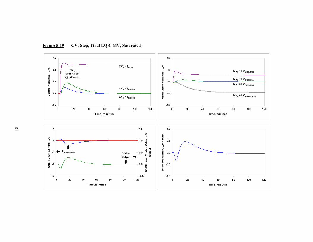
Figure 5-19 CV3 Step, Final LQR, MV1 Saturated
-0.4
0.0
0.4
0.8
1.2
0 20 40 60 80 100 120
Time, minutes
Con
trol
Var
iabl
es,
∆o C
CV2 = TR1B2,IN
CV1 = TR1B1,IN
CV3 = TR2,INCV3
UNIT STEP @ t=2 min.
-16
-8
0
8
16
0 20 40 60 80 100 120
Time, minutes
Man
ipul
ated
Var
iabl
es,
∆%
MV2 = HVG/G,SHELL
MV4 = HVWHBII,STEAM
MV1 = HVR1PH,TUBE
MV3 = HVWHBI,TUBE
-3
-2
-1
0
1
0 20 40 60 80 100 120
Time, minutes
WH
B II
Lev
el C
ontr
ol, ∆
%
-0.5
0.0
0.5
1.0
1.5
WH
BII
Leve
l Con
trol
Val
ve,
∆%
O
utpu
tLWHBII,SHELL Valve
Output
-1.0
-0.5
0.0
0.5
1.0
0 20 40 60 80 100 120
Time, minutes
Stea
m P
rodu
ctio
n, ∆
tonn
e/hr
84
85
5.5. Discussion
By careful selection of the control variables, both the linear LQR and PID controllers are able to
effectively control a known nonlinear process. Tables 5-3 and 5-4 summarize the PID and LQR
controller performance. Comparison of these controllers can be found in Table 5-5.
Table 5-3 looks at the controllers with MV1, MV2 and MV3 involved in the control
strategy. Performance of both the PID and LQR controllers is exceptionally good. Settling times
are fast, process disturbances introduced by changing setpoints are relatively small and steam
overshoot is within specifications. Without introducing a quantitative measurement, such as
ITAE, with penalties on changing steam production and MV movement, it is difficult to
differentiate between the results. Noting that an optimizer may only run a few times per day with
a new setpoint, the differences between the two controllers are not considered to be significant.
Similarly, Table 5-4 looks at the control performance with MV2, MV3 and MV4, actively
involved in the control matrix. MV4, which has a larger impact on steam production and notably
slower dynamics than the other MVs, inherently introduces a layer of complexity to the control
problem. In all cases, the time required for these highly interactive loops to return to steady-state
after a CV unit step is significantly less for the LQR. After a unit step in CV3, the settling time for
PID control is over 1 hour longer than the time for the LQR controller to reach steady-state.

Table 5-3 Comparative Controller Behaviour with MV4 Saturated
Control Variable
(∆OC)
Control Type
CV Response
Time (minutes)
CV Settling
Time (minutes)
Process Settling
Time (minutes)
CV1 Dev’n (∆OC)
CV2 Dev’n (∆OC)
CV3 Dev’n (∆OC)
∆MSTEAM
(∆tonne/hr)
PID 4.3 4.3 4.3 0.00 0.15 0.00 0.04∆CV1 = 1 LQR 5.6 5.6 5.6 0.00 0.19 0.05 0.06PID 0.5 1.2 4.6 0.43 0.04 0.03 0.58∆CV2 = 1 LQR 7.5 7.5 7.5 0.26 0.00 0.17 0.57PID 1.0 1.0 1.0 0.00 0.01 0.00 0.28∆CV3 = 1 LQR 1.6 1.6 5.6 0.05 0.09 0.00 0.28
Table 5-4 Comparative Controller Behaviour with MV1 Saturated
Control Variable
(∆OC)
Control Type
Response Time
(minutes)
CV Settling
Time (minutes)
Process Settling
Time (minutes)
CV1 Dev’n (∆OC)
CV2 Dev’n (∆OC)
CV3 Dev’n (∆OC)
∆MSTEAM
(∆tonne/hr)
PID 3.3 3.3 22.8 0.00 0.30 0.01 0.21∆CV1 = 1 LQR 11.3 11.3 11.3 0.00 -0.16 -0.09 -0.08PID 106.5 106.5 106.5 0.02 0.00 0.00 1.00LQR 70.5 70.5 70.5 0.38 0.00 0.09 1.00
∆CV2 = 1
LQR–Model 33.4 59.6 59.6 0.41 0.06 0.09 0.90PID 0.9 0.9 90.5 0.05 0.40 0.00 0.97∆CV3 = 1 LQR 3.1 27.4 27.4 0.21 0.36 0.03 0.79
86

87
The advantages and disadvantages of the characteristics of each controller are
summarized in Table 5-5. The complexity of the two controllers is also a determining factor in
selecting the preferred control scheme, PID or LQR. While LQR performance is superior
compared to PID control, implementation in this case is not considered practical based on the
incremental effort required to develop, maintain and train operations. Further use of
HVWHBII,STEAM in the control strategy demonstrates marginal performance. Prior to implementing a
controller with this MV, additional tests should be carried out, including evaluating the
controller’s ability to reject noise and process disturbances. Based on these results, PID control is
recommended, preferably excluding HVWHBII,STEAM as a manipulated variable.
Table 5-5 Comparative Controller Characteristics
Control Type PID LQR
1. Well known industry standard. 1. Inherently considers process as single control problem with CVs to be resolved simultaneously.
2. Tools and control algorithms readily available.
2. Control algorithm weights MV adjustments.
3. Single loop tuning relatively simple.
4. Model identification based on three control variables.
Advantages
5. Easy to drop single CV from control scheme.
1. Considers process as three distinct control problems to be resolved independently.
1. Technology relatively complex.
2. Tuning of multiple loops with interaction done iteratively.
2. Custom programming required to implement LQR algorithm.
3. Controller based on a linearized process.
3. Three control matrices tuned iteratively.
4. Model identification based on 34 state space variables.
5. Custom programming required to drop CV from control scheme.
Disadvantages
6. Controller based on a linearized process.
Control considerations not included here are controller stability and process noise.
Typically the stability of the controller over different operations needs to be explored.
Additionally if noise is introduced in the process, controller results may vary slightly, particularly
with respect to the steam system.

88
CHAPTER 6
SUMMARY AND CONCLUSIONS
The growing demand for nitrogen fertilizer in agriculture has renewed interest in control
applications for ammonia production. The objective of this thesis is to explore these automation
prospects and technologies to exploit these opportunities at Saskferco Products Inc. The ammonia
synthesis unit is chosen as the focal point of these studies. While some research has been done on
similar units, it is neither exhaustive nor entirely clear that other means of control would not
achieve similar results, with less overhead required for implementation and maintenance.
Additionally, known nonlinearities in the ammonia synthesis unit offer the chance to investigate
the applicability of conventional linear control methods to a nonlinear process.
6.1. Area of Study
A dynamic model of the ammonia synthesis unit is developed to provide insight into the process
operation and a platform for optimization and control studies. To improve the accuracy of the
model for these studies, dynamic update of a reaction fit parameter is investigated using historical
data. Parameter estimation is intended to account for model mismatch, changing catalyst activity
and diffusion limitations. To this end, a new term referred to as the catalyst effectiveness
parameter is introduced into the Temkin-Pyshev reaction equation, biasing the reaction kinetics of
the rate-limiting forward reaction. Update of this parameter using variations in the least squares
algorithm is studied to determine the most suitable update method.
Based on this model, several optimization studies are performed, including normal
operation, seasonal operation and operation during periods of reduced catalyst activity. The
objective function is to maximize overall conversion of synthesis gas to ammonia for each pass
through the converter beds. Increased conversion potentially allows increased make-up gas feed,
and a more efficient process based on reduced synthesis gas recycle. Given the fast dynamics of
the process relative to the process disturbance frequency, optimization studies are based on the
steady-state operation of the process. Process control to enforce optimization results is
investigated for PID and LQR control strategies using 3 CVs and 4 MVs. A maximum overshoot
in steam production of 1 tonne/hr per 1 oC setpoint change is imposed. As part of the plant’s
protection system, the WHB level control is not included in this advanced control application.

89
This thesis took the standard approach for level control by implementing a proportional
controller, despite limitations as a regulatory controller.
6.2. Results
Process model results, with fit parameters in the model, reveal a good fit between plant data and
model predictions. Nonlinear relationships in the converters and known problems in the control of
the WHB level are substantiated.
The results of the parameter update problem found the recursive least squares algorithm,
to be the most accurate and practical approach. Using 3 parameters to estimate 4 process
measurements, the recursive least squares method demonstrated the best overall accuracy, with
the least variation in the parameter results. Computer resources in this case are approximately 6 %
of other least squares formulations. Interestingly the weighted least squares method typically
sacrificed the R1B1 inlet temperature to achieve results. The major drawback of this method is
that it is based on difference variables. Accordingly, it must be coupled with another method,
such as the sum of squares, to find reasonable initial conditions and to circumvent model drift.
Studies around the sum of squares parameter update method uncover a strong relationship
between the parameter update value and the process H/N ratio. These results expose a limitation
in the process model, which over-penalizes ammonia conversion at higher H/N ratios.
Results of the optimization studies identified potential benefits of approximately $180
k/year. In all cases, it is found that the R1 preheater bypass valve is typically constrained in the
closed position. It is observed that a reduced optimization model on the last converter bed could
achieve 70 % of these benefits.
Analysis of summer versus winter operation reveals some interesting relationships.
Typically Saskferco operates at reduced rates in the summer months due to process limitations
aggravated by ambient temperatures. Increased ammonia conversion in the summer is partially
attributed to a reduction of inerts in the feed and also possibly to the reduction in catalyst
diffusion limitations with reduced throughput. Optimal converter temperatures are on average 3 oC, 5 oC and 6 oC colder in beds one, two and three respectively during the summer months
compared to winter.
Results of a post optimality analysis indicate a conversion “dead zone” in the region
surrounding the optimal reactor inlet temperature. This information can ultimately be used to
operate the plant a safe margin above the calculated optimum temperature without significant
penalties or to accept/reject changes in the optimization results depending on the magnitude of the
change. Results are unable to confirm the optimum H/N ratio given in literature.

90
Loop paring for PID control, using the RGA, is contrary to what might have been
anticipated given the process layout. The R1B2 inlet temperature is paired with the two valves
upstream of R1B1 as a split range controller, while the R1B1 temperature is paired with the
converter one preheater bypass valve. PID control on the nonlinear process model is relatively
simple to implement and is able to effectively satisfy the control criteria. Performance of the
R1B2 inlet temperature with the WHB II BFW split valve is marginal. A settling time of 107
minutes is observed, with an overshoot in steam production of 1 tonne/hour when this CV is
perturbed with a unit step.
Design of the optimal controller, LQR, is also straightforward. The main difficulty with
this method is to formulate an appropriate performance index to meet the control criterion and to
address steady-state errors and controller stability issues. Tuning of this controller encompasses 3
weighting matrices that are solved iteratively. Input saturation of the gas-gas exchanger bypass is
handled by dropping this MV from the control matrix. The worst performance is observed in the
R1B2 inlet temperature when stepped with the gas-gas exchanger bypass valve saturated, with a
settling time of 71 minutes.
6.3. Conclusions
It is concluded that the opportunity exists at Saskferco to improve control and optimization in the
ammonia synthesis loop. Implementation based on conventional and modest automation
techniques is determined to be the most feasible, achieving the majority of these benefits.
Linear LQR and PID controllers are able to successfully control a known nonlinear
process by judicious selection of the control variables. Performance of the LQR for highly
interactive loops is considered superior to the PID control strategy, based on controller settling
times. However, while LQR control results are encouraging, implementation is not considered to
be practical based on the incremental effort required to program, tune, maintain and train
operations compared to PID control. Depending on optimization frequency, effective benefits
between these servo controllers could be considered financially insignificant.
Based on optimization results, indicating saturation of the R1PH bypass valve, PID
control on the R1B1 inlet temperature would be meaningless. Further, PID control of the R1B2
inlet temperature controller is also not considered feasible based on marginal performance of this
loop with the WHB BFW split valve. Significant detuning is necessary to reduce impact on the
steam system, resulting in long settling times. Control benefits of $54 k/year are outweighed by
potential oscillations in the steam system (and possible plant trip scenarios).
91
While existing MVC ammonia synthesis controllers have been demonstrated on quench
converters, with different MVs available, installation of MVC for ammonia synthesis is
questioned, considering the relative benefits of simpler control strategies.
6.4. Recommendations
Further research to investigate the comparative performance of the PID and LQR controllers, as
regulatory controllers, subject to noise and disturbance variables, should be explored. Results and
conclusions of this thesis are based on the servo control response of PID and LQR systems.
While this thesis focuses on the ammonia synthesis loop at Saskferco, it is noted that
additional control opportunities in the ammonia plant may exist in upstream units. Given rising
energy costs, opportunities in the UHDE methane reformer may prove attractive. It is noted that
similar reformer control applications have been implemented[20],[22].
As a final submission, the following recommendations are made for Saskferco
operations.
1. On-line optimization of the R2 inlet temperature.
2. On-line optimization of the R1 inlet temperatures operated in advisory mode.
Results would be available as an operational guide and to alarm temperatures
below optimal conditions, where potential loss of the reaction exists.
3. Parameter updates to complement process optimizers.
Implementation would be achieved using a weighted least squares approach
augmented with the sum of squares, for initial conditions and to prevent model
drift. Ammonia conversion soft sensors through each converter bed would be
beneficial by-products of these efforts.
4. R2 inlet temperature PID control operating in conjunction with the R2 optimizer.
Site issues relating to the WHB I bypass control valve will need to be addressed.
5. Investigation of improved control strategies on the WHB II level controller.

92
BIBLIOGRAPHY
[1] M. Appl. Ammonia, Principles and Industrial Practice. Wiley-VCH, Weinheim, 1999.
[2] H. Bakermeier, T. Huberich, R. Krabetz, W. Liebe, M. Schunk, Ullmann’s Encyclopedia of
Industrial Chemistry, Ammonia. A2, VCH Verlagsgesellschaft, 1996.
[3] A. Bertucco, M. Barolo and G. Soave. Estimation of Chemical Equilibria in High-Pressure
Gaseous Systems by a Modified Redlich-Kwong-Soave Equation of State. Ind. Eng. Chem.
Res, 34:3159-3165, 1995.
[4] B.W. Bequette. Process Dynamics, Modelling, Analysis and Simulation. Prentice Hall Inc.,
Upper Saddle River, NJ, 1998.
[5] S. Bittanti, A.J. Laub and J.C. Willems. The Riccati Equation. Springer-Verlag New York
Inc., New York, 1991.
[6] W.L. Brogan. Modern Control Theory. Prentice Hall Inc., Upper Saddle River, NJ, 1991.
[7] D.R. Coughanowr. Process Systems Analysis and Control. Second Edition. McGraw-Hill
Inc., New York, 1991.
[8] J.J. D’Azzo and C.H. Houpis. Linear Control System Analysis and Design. Conventional
and Modern. Second Edition. McGraw-Hill Inc, New York, 1981.
[9] J.M. Douglas. Process Dynamics and Control, Volume 2, Control Systems Synthesis. pages
291-293, Prentice Hall, Ingelwood Cliffs, NJ, 1972.
[10] N. Draper and H. Smith. Applied Regression Analysis, Second Edition. John Wiley & Sons,
Inc., 1966.
[11] T.F. Edgar and D.M. Himmelblau. Optimization of Chemical Processes. McGraw-Hill Inc.,
New York, 1988.
[12] B. Edmondson, Saskferco Products Inc. Technical Director, Belle Plaine, SK. Personal
Communications, 1999.

93
[13] S. S. Elnashaie, M. E. Abashar and A. S. Al-Ulbaid. Simulation and Optimization of an
Industrial Ammonia Reactor. Ind. Eng. Chem. Res., 27:2015-2022, 1988.
[14] B. Friedland. Control System Design. An Introduction to State-Space Methods. McGraw-
Hill Inc., New York, 1986.
[15] N. Ganesh, L.T. Biegler. A Reduced Hessian Strategy for Sensitivity Analysis of Optimal
Flowsheets. AIChe Journal. 33(2):282-296, February 1987.
[16] J.P. Holman. Heat Transfer, Seventh Edition. McGraw-Hill Inc., New York, 1990
[17] B.R. Hope, P. K. Robertson. Confidential Disclosure Agreement Between Saskferco and
University of Alberta. Alberta, 2001.
[18] A. Hugo. Limitations of Model Predictive Controllers. Hydrocarbon Processing, pages 83-
88, January 2000.
[19] L. Kane. Advanced Process Control Strategies 1993. Hydrocarbon Processing, pages 84-85,
September 1993.
[20] E. Kharbat. Successful Application of Adaptive Technologies to Ammonia Reformers.
Ammonia Plant Safety and Related Facilities, 38:279-285, 1998.
[21] J.N. Little, C.M. Thompson, P. Gahinet, Control System Toolbox for Use With Matlab,
User’s Guide. The MathWorks Inc., Natick MA, 4.2, 1992-1999.
[22] R. Lin, R. de Boer and B. Poe. Optimize Ammonia Plant Operation. Hydrocarbon
Processing, pages 91-100, June 1999.
[23] L. Ljung and T. Soderstrom. Theory and Practice of Recursive Identification. The MIT
Press, Cambridge, Massachusetts, 1983.
[24] W.G. Mallard and P.J. Linstrom, Eds. NIST Chemistry WebBook, NIST Standard Reference
Database Number 69. http://webbook.nist.gov. National Institute of Standards and
Technology, Gaithersburg MD, February 2000.
[25] B. Mansson and B. Andresen. Optimal Temperature Profile for an Ammonia Reactor. Ind.
Eng. Chem. Process Des. Dev., 25:59-65, 1986.

94
[26] J. Markos and M. Barto. Optimization Method for Balance Adjustment in Large Chemical
Process Systems. Chem. Eng. Process., 30:45-50, 1991.
[27] T.E. Marlin. Process Control Designing Processes for Control Systems for Dynamic
Performance, McGraw-Hill Inc., New York, 1995.
[28] S.A. Matthews. Process Plant Productivity Improvement through Neural Network
Applications. ISA TECH EXPO Technology Update Conference Proceedings. 1(2):157-166,
ISA, Research Triangle Park, NC, 1997
[29] A. Mihajlov, B. Djordjevic and A. Tasic. Calculation of Enthalpy and Entropy of Gases by
Modified Redlich-Kwong Equation of State. Hungarian Journal of Industrial Chemistry,
9:407-416, 1981.
[30] K. Mishima, J. Sugino, M. Ueno, K. Matsuyama and M. Nagatani. Correlation of
Solubilities for CO2 and NH3 in H2O Using Soave-Redlich-Kwong Equation of State with
MHV2 Mixing Rule. Journal of Chemical Engineering of Japan. 28(2):144-147, 1995.
[31] M. Munro. Beware the Green Peril. National Post. Hollinger/Canwest Publications, 24-
April, 2001
[32] D.Y. Murzin and A.K. Avetisov. Kinetics of Ammonia Synthesis Close to Equilibrium. Ind.
Eng. Chem. Res., 36:4779-4783, 1997.
[33] L. Naess, A. Mjaavatten and J.O, Li. Using Dynamic Process Simulation from Conception
to Normal Operation of Process Plants. Computers Chem. Engng., 17(5/6):585-600, 1993.
[34] L.M. Patnaik, N. Viswanadham and I.G. Sarma. Design of Multiloop Controllers for an
Ammonia Reactor. IEEE Transactions on Industrial Electronics and Control
Instrumentation, 28(4):253-358, 1981.
[35] L.M. Patnaik, N. Viswanadham and I.G. Sarma. Hierarchical Control of an Ammonia
Reactor. IEEE Transactions of Systems, Man and Cybernetics, 12(6):919-924,
November/December 1982.
[36] E. A. Robinson. Least Square Regression Analysis in Terms of Linear Algebra. Goose Pond
Press., Houston, 1981.
95
[37] J. M. Smith and H. C. Van Ness. Introduction to Chemical Engineering Thermodynamics.
Fourth Edition. McGraw-Hill, Inc. New York, 1987.
[38] G. Soave. Direct Calculation of Pure-Compound Vapour Pressures through Cubic
Equations of State. Fluid Phase Equilibria, 31:203-207, 1986.
[39] G. Soave, M. Barolo and A. Bertucco. Estimation of high-pressure fugacity coefficients of
pure gaseous fluids by a modified SRK equation of state. Fluid Phase Equilibria, 91:87-
100, 1993.
[40] D. Tilman, J. Fargione, B. Wolff, C. D’Antonio, A. Dobson, R. Howarth, D. Schindler, W.
H. Schlesinger, D. Simberloff, and D. Swackhamer. Forecasting Agriculturally Driven
Global Environmental Change. SCIENCE, 292:281-284, April 2001.
[41] M. V. Twigg. Catalyst Handbook. Second Edition. Manson Publishing, London, 1996.
[42] S.R. Upreti and K. Deb. Optimal Design of an Ammonia Synthesis Reactor Using Genetic
Algorithms. Computers Chem. Engng., 21(1):87-92, 1997.
[43] N. Viswanadham, L.M. Patnaik and I.G. Sarma. Robust Multivariable Controllers for a
Tubular Ammonia Reactor. Transactions of the ASME. 101:290-298, December 1979.
[44] C. Ying and B. Joseph. Performance and Stability Analysis of LP-MPC and QP-MPC
Cascade Control Systems. AIChe Journal, 34(7):1521-1534, July 1999.

96
APPENDIX A
PLANT DATA
Shift averages for February and March were collected from the Saskferco information system.
This data is used to fit the Simulink process model, in the parameter fit evaluations and for
comparison of operation to optimization results.
Table A-1 Plant Data
Date VIN,SG PIN,SG yIN,NH3 yIN,N2 yIN,H2 yIN,HE yIN,AR yIN,CH4
k-sm3/hr MPag vol % vol % vol % vol % vol % vol %
01-Feb-99 07:00 729.30 18.90 2.23 20.46 61.85 0.99 2.90 11.2701-Feb-99 19:00 731.11 18.85 2.23 20.60 61.55 0.99 2.90 11.2902-Feb-99 07:00 736.00 18.87 2.20 20.48 61.32 0.98 2.88 11.7502-Feb-99 19:00 731.31 18.79 2.19 20.55 61.64 0.97 2.90 11.3603-Feb-99 07:00 731.49 18.83 2.19 20.52 61.60 0.97 2.90 11.4003-Feb-99 19:00 732.93 18.75 2.28 20.63 61.78 1.01 2.91 11.1204-Feb-99 07:00 721.86 18.60 2.20 20.61 61.85 1.04 2.91 10.9704-Feb-99 19:00 726.87 18.75 2.23 20.59 61.95 1.06 2.91 10.8905-Feb-99 07:00 731.18 18.84 2.23 20.63 61.80 1.05 2.90 11.0805-Feb-99 19:00 733.36 18.73 2.21 20.60 61.79 1.05 2.90 11.1206-Feb-99 07:00 731.94 18.75 2.19 20.63 61.78 1.05 2.91 11.0506-Feb-99 19:00 728.10 18.83 2.24 20.55 61.90 1.03 2.91 11.0107-Feb-99 07:00 728.95 18.89 2.21 20.03 62.07 1.01 2.90 11.3207-Feb-99 19:00 720.57 19.06 2.24 18.31 63.96 0.99 2.83 11.2808-Feb-99 07:00 732.44 18.95 2.22 19.96 61.83 1.00 2.87 11.7008-Feb-99 19:00 734.57 18.82 2.23 20.42 61.34 0.96 2.88 11.7509-Feb-99 07:00 737.74 18.83 2.22 20.48 61.46 0.95 2.89 11.6609-Feb-99 19:00 737.54 18.89 2.24 20.46 61.42 0.95 2.88 11.7210-Feb-99 07:00 733.93 18.93 2.27 20.42 61.32 0.92 2.88 11.7210-Feb-99 19:00 736.05 18.82 2.24 20.47 61.15 0.94 2.83 12.0011-Feb-99 07:00 736.98 18.86 2.25 20.38 61.07 1.01 2.82 12.0811-Feb-99 19:00 741.89 18.88 2.26 20.29 60.95 1.02 2.89 12.1112-Feb-99 07:00 746.09 18.92 2.26 20.32 60.90 1.07 2.98 12.0712-Feb-99 19:00 748.77 18.97 2.27 20.20 60.82 1.08 3.00 12.2313-Feb-99 07:00 745.79 19.05 2.31 20.24 60.86 1.04 2.99 12.2413-Feb-99 19:00 744.39 19.01 2.31 20.45 60.68 1.03 2.99 12.1714-Feb-99 07:00 743.93 19.04 2.33 20.39 60.47 1.05 2.97 12.3114-Feb-99 19:00 742.94 18.92 2.28 20.49 60.50 1.06 2.94 12.2815-Feb-99 07:00 741.86 18.91 2.27 20.55 60.57 1.06 2.93 12.2415-Feb-99 19:00 745.40 18.87 2.27 20.49 60.55 1.06 2.92 12.3216-Feb-99 07:00 741.93 18.90 2.27 20.55 60.66 1.04 2.89 12.2116-Feb-99 19:00 741.65 18.90 2.29 20.59 60.61 1.02 2.89 12.2217-Feb-99 07:00 741.19 18.86 2.24 20.52 60.67 1.01 2.87 12.2917-Feb-99 19:00 738.73 18.87 2.28 20.58 60.81 1.00 2.89 12.0518-Feb-99 07:00 741.24 18.94 2.26 20.24 60.80 1.00 2.91 12.3918-Feb-99 19:00 739.42 18.95 2.30 20.04 60.99 1.05 2.94 12.3119-Feb-99 07:00 737.33 18.99 2.31 20.08 61.13 1.06 2.95 12.1019-Feb-99 19:00 739.26 19.04 2.34 20.01 61.07 1.14 2.94 12.11
97
Date VIN,SG PIN,SG yIN,NH3 yIN,N2 yIN,H2 yIN,HE yIN,AR yIN,CH4
k-sm3/hr MPag vol % vol % vol % vol % vol % vol %
20-Feb-99 07:00 744.15 19.15 2.38 19.79 61.05 1.20 2.92 12.2720-Feb-99 19:00 743.52 19.14 2.38 19.40 61.23 1.16 2.86 12.5621-Feb-99 07:00 739.19 19.08 2.34 19.55 61.18 1.15 2.83 12.5721-Feb-99 19:00 734.56 18.99 2.31 19.62 61.69 1.16 2.88 11.9322-Feb-99 07:00 737.32 19.11 2.37 19.61 61.52 1.15 2.89 12.0722-Feb-99 19:00 735.96 18.98 2.28 19.57 61.66 1.15 2.90 12.0723-Feb-99 07:00 731.47 18.95 2.27 19.56 61.61 1.12 2.87 12.1526-Feb-99 19:00 729.97 18.75 2.38 21.78 60.72 0.96 2.87 10.9127-Feb-99 07:00 736.26 18.84 2.28 20.04 62.37 0.94 2.84 11.1527-Feb-99 19:00 737.44 18.90 2.26 19.57 62.58 0.97 2.83 11.4028-Feb-99 07:00 733.93 18.82 2.25 19.68 62.83 0.99 2.84 11.0228-Feb-99 19:00 733.40 18.89 2.27 19.49 62.99 0.98 2.82 11.0701-Mar-99 07:00 736.66 18.86 2.24 19.64 62.64 0.98 2.81 11.2901-Mar-99 19:00 737.44 18.87 2.26 19.61 62.52 0.97 2.80 11.4502-Mar-99 07:00 735.83 18.79 2.23 19.65 62.83 0.96 2.78 11.1502-Mar-99 19:00 737.45 18.81 2.23 19.63 62.76 0.95 2.79 11.2903-Mar-99 07:00 740.15 18.83 2.24 19.76 62.37 0.93 2.79 11.5403-Mar-99 19:00 739.06 18.87 2.29 20.03 62.04 0.92 2.80 11.5304-Mar-99 07:00 738.20 18.93 2.31 20.02 62.12 0.93 2.77 11.4904-Mar-99 19:00 742.61 19.05 2.36 19.95 61.87 0.88 2.74 11.8305-Mar-99 07:00 740.64 18.96 2.33 19.99 61.95 0.88 2.74 11.7305-Mar-99 19:00 744.95 18.95 2.28 19.87 61.73 0.98 2.77 12.0206-Mar-99 07:00 738.05 18.92 2.27 19.80 62.49 1.01 2.77 11.3006-Mar-99 19:00 738.27 18.91 2.28 19.78 62.32 1.01 2.77 11.4307-Mar-99 07:00 738.00 18.86 2.26 19.74 62.33 1.03 2.76 11.5007-Mar-99 19:00 734.86 18.90 2.27 19.81 62.51 1.06 2.75 11.2008-Mar-99 07:00 736.10 18.98 2.33 19.75 62.21 1.07 2.72 11.5308-Mar-99 19:00 739.16 19.02 2.34 19.61 61.92 1.04 2.70 12.0109-Mar-99 07:00 738.18 19.01 2.35 19.65 61.96 1.03 2.69 11.9409-Mar-99 19:00 744.07 19.00 2.44 19.73 63.83 0.91 2.80 9.8910-Mar-99 07:00 746.64 18.91 2.51 20.43 64.35 0.88 2.95 8.5010-Mar-99 19:00 743.25 18.90 2.48 19.91 64.89 0.89 2.93 8.5111-Mar-99 07:00 743.89 18.83 2.47 19.85 64.86 0.93 2.96 8.5611-Mar-99 19:00 744.77 18.84 2.46 20.30 64.36 0.92 3.00 8.5912-Mar-99 07:00 751.80 18.93 2.47 20.13 64.33 0.95 3.10 8.6312-Mar-99 19:00 748.89 18.99 2.51 20.17 64.52 0.91 3.09 8.4113-Mar-99 07:00 754.32 18.98 2.50 20.07 64.23 0.90 3.09 8.8513-Mar-99 19:00 755.02 19.05 2.54 20.03 64.09 0.86 3.08 9.0114-Mar-99 07:00 757.02 19.06 2.52 20.03 63.96 0.85 3.08 9.1914-Mar-99 19:00 752.85 19.12 2.55 19.61 64.33 0.81 3.06 9.2415-Mar-99 07:00 750.21 19.19 2.53 19.00 65.04 0.80 3.00 9.2415-Mar-99 19:00 753.08 19.14 2.52 19.28 64.55 0.83 3.00 9.4416-Mar-99 07:00 757.08 19.08 2.50 19.44 64.20 0.83 3.03 9.6316-Mar-99 19:00 738.68 18.92 2.51 19.57 64.77 0.81 3.12 8.8317-Mar-99 07:00 755.70 19.08 2.51 19.52 64.28 0.87 3.03 9.4217-Mar-99 19:00 764.68 19.14 2.47 19.39 63.90 0.82 3.01 10.0418-Mar-99 07:00 764.38 19.12 2.43 19.38 63.94 0.86 3.00 10.0218-Mar-99 19:00 759.44 19.18 2.46 19.44 64.12 0.90 3.04 9.6819-Mar-99 07:00 752.73 19.08 2.46 19.51 64.49 0.91 3.04 9.2219-Mar-99 19:00 754.45 19.20 2.52 19.47 64.23 0.89 3.03 9.4820-Mar-99 07:00 755.09 19.12 2.48 19.47 64.26 0.87 3.02 9.5220-Mar-99 19:00 756.03 19.13 2.46 19.08 65.06 0.82 2.99 9.1921-Mar-99 07:00 758.58 19.07 2.46 18.84 65.89 0.83 2.93 8.6621-Mar-99 19:00 758.49 19.11 2.43 18.47 66.38 0.78 2.93 8.62

98
Date VIN,SG PIN,SG yIN,NH3 yIN,N2 yIN,H2 yIN,HE yIN,AR yIN,CH4
k-sm3/hr MPag vol % vol % vol % vol % vol % vol %
22-Mar-99 07:00 758.42 19.07 2.42 18.43 66.37 0.81 2.93 8.6622-Mar-99 19:00 761.70 19.12 2.43 18.42 66.26 0.79 2.93 8.7823-Mar-99 07:00 764.07 19.10 2.44 18.35 66.01 0.83 2.91 9.0823-Mar-99 19:00 763.06 19.13 2.48 18.34 66.02 0.84 2.93 9.0224-Mar-99 07:00 761.94 19.02 2.41 18.36 66.13 0.87 2.91 8.9624-Mar-99 19:00 759.38 19.05 2.43 18.39 66.22 0.88 2.93 8.8025-Mar-99 07:00 759.50 19.05 2.43 18.37 66.14 0.87 2.93 8.9025-Mar-99 19:00 757.91 19.13 2.48 18.35 66.24 0.85 2.92 8.7926-Mar-99 07:00 757.59 19.26 2.55 17.49 67.06 0.88 2.98 8.6726-Mar-99 19:00 739.92 19.27 2.48 16.32 68.93 0.85 2.82 8.2127-Mar-99 07:00 719.36 19.09 2.44 15.86 70.28 0.93 2.70 7.4327-Mar-99 19:00 721.97 19.01 2.44 16.61 69.50 0.89 2.72 7.4828-Mar-99 07:00 741.92 18.96 2.45 18.33 67.00 0.87 2.79 8.1628-Mar-99 19:00 748.17 19.01 2.47 18.48 66.49 0.81 2.78 8.6129-Mar-99 07:00 745.54 18.91 2.45 18.56 66.78 0.78 2.80 8.2529-Mar-99 19:00 741.59 18.95 2.47 18.21 67.15 0.80 2.81 8.1930-Mar-99 07:00 742.18 18.97 2.46 17.90 67.30 0.81 2.80 8.3430-Mar-99 19:00 743.73 19.15 2.48 16.98 67.98 0.81 2.84 8.5331-Mar-99 07:00 756.58 19.16 2.51 17.96 66.39 0.91 2.95 8.9231-Mar-99 19:00 768.92 19.20 2.54 18.72 65.61 0.91 3.04 8.8101-Jul-99 07:00 708.91 18.89 2.57 15.58 68.79 1.30 2.82 8.9501-Jul-99 19:00 708.31 19.14 2.54 14.21 70.17 1.27 2.75 9.0602-Jul-99 07:00 705.52 19.05 2.49 14.44 70.02 1.37 2.76 8.9202-Jul-99 19:00 704.06 19.13 2.59 14.37 69.78 1.37 2.75 9.1403-Jul-99 07:00 705.02 19.02 2.49 15.34 68.47 1.34 2.74 9.6203-Jul-99 19:00 703.48 19.22 2.55 14.22 70.07 1.26 2.71 9.1904-Jul-99 07:00 700.80 19.18 2.47 14.12 70.33 1.29 2.76 9.0304-Jul-99 19:00 700.19 19.18 2.44 14.09 70.50 1.26 2.67 9.0405-Jul-99 07:00 707.49 19.24 2.42 14.28 69.91 1.28 2.67 9.4405-Jul-99 19:00 698.34 19.19 2.62 14.51 69.90 1.25 2.66 9.0706-Jul-99 07:00 719.74 19.22 2.54 14.56 69.05 1.25 2.70 9.8906-Jul-99 19:00 712.17 19.25 2.66 14.27 69.77 1.19 2.70 9.4107-Jul-99 07:00 718.19 19.15 2.55 14.55 69.52 1.23 2.74 9.4107-Jul-99 19:00 711.63 19.26 2.69 13.91 70.31 1.26 2.71 9.1208-Jul-99 07:00 712.74 19.21 2.75 14.57 69.19 1.29 2.69 9.5008-Jul-99 19:00 705.36 19.05 2.57 14.83 69.26 1.26 2.74 9.3409-Jul-99 07:00 720.70 19.09 2.56 15.11 68.50 1.28 2.79 9.7609-Jul-99 19:00 713.11 19.05 2.63 15.20 68.92 1.19 2.79 9.2810-Jul-99 07:00 710.72 19.05 2.53 14.65 69.44 1.31 2.81 9.2710-Jul-99 19:00 703.11 19.19 2.67 13.81 70.70 1.29 2.74 8.7911-Jul-99 07:00 703.78 19.10 2.63 14.32 70.14 1.35 2.77 8.8011-Jul-99 19:00 694.48 19.31 2.78 13.12 71.65 1.37 2.72 8.3712-Jul-99 07:00 705.80 19.26 2.77 14.51 69.26 1.47 2.97 9.0212-Jul-99 19:00 694.73 19.18 2.81 14.49 69.66 1.49 2.99 8.5613-Jul-99 07:00 704.72 19.14 2.75 15.13 68.65 1.50 2.99 8.9713-Jul-99 19:00 707.54 19.15 2.67 14.83 68.90 1.44 2.92 9.2414-Jul-99 07:00 709.98 19.20 2.63 14.49 69.18 1.48 2.94 9.2914-Jul-99 19:00 711.06 19.24 2.70 14.36 69.11 1.52 2.93 9.3815-Jul-99 07:00 705.91 19.22 2.73 14.35 69.20 1.51 2.91 9.3015-Jul-99 19:00 625.76 18.20 2.94 15.68 67.87 1.49 3.24 8.7716-Jul-99 07:00 521.21 17.01 3.11 16.82 66.48 1.92 3.58 8.0816-Jul-99 19:00 567.32 17.43 3.12 17.77 64.42 2.21 3.74 8.7517-Jul-99 07:00 649.17 17.90 2.65 18.83 65.06 1.81 3.10 8.5517-Jul-99 19:00 681.91 18.01 2.57 19.54 63.80 1.52 3.18 9.40

99
Date VIN,SG PIN,SG yIN,NH3 yIN,N2 yIN,H2 yIN,HE yIN,AR yIN,CH4
k-sm3/hr MPag vol % vol % vol % vol % vol % vol %
18-Jul-99 07:00 706.28 18.80 2.62 15.86 67.58 1.38 2.89 9.6818-Jul-99 19:00 709.90 19.14 2.68 14.46 69.12 1.41 2.89 9.4419-Jul-99 07:00 706.62 18.86 2.67 15.37 68.36 1.51 2.90 9.1819-Jul-99 19:00 698.34 19.18 2.67 13.99 70.30 1.47 2.78 8.7920-Jul-99 07:00 699.85 19.14 2.60 14.34 69.61 1.56 2.83 9.0620-Jul-99 19:00 692.70 19.25 2.80 14.33 69.53 1.51 2.81 9.0221-Jul-99 07:00 696.05 19.08 2.84 15.07 68.64 1.50 2.86 9.0921-Jul-99 19:00 684.88 19.13 2.86 14.89 69.36 1.37 2.87 8.6522-Jul-99 07:00 703.24 19.19 2.75 15.02 68.34 1.42 2.92 9.5522-Jul-99 19:00 679.11 19.12 2.85 14.67 69.75 1.23 2.80 8.6923-Jul-99 07:00 701.54 19.08 2.67 15.26 68.45 1.27 2.87 9.4723-Jul-99 19:00 699.54 19.19 2.85 15.07 68.49 1.26 2.87 9.4624-Jul-99 07:00 654.16 18.25 2.75 16.62 66.35 1.63 3.76 8.9024-Jul-99 19:00 695.63 19.17 2.88 15.26 67.82 1.55 2.97 9.5225-Jul-99 07:00 689.65 18.97 2.83 15.66 68.33 1.35 2.79 9.0425-Jul-99 19:00 700.35 19.07 2.72 15.34 68.31 1.27 2.84 9.5326-Jul-99 07:00 712.46 18.87 2.47 16.36 67.10 1.28 2.91 9.8626-Jul-99 19:00 709.28 19.09 2.57 14.77 68.85 1.24 2.86 9.7227-Jul-99 07:00 711.78 19.15 2.53 14.53 68.95 1.36 2.86 9.7727-Jul-99 19:00 699.34 19.21 2.73 14.29 69.35 1.39 2.81 9.4328-Jul-99 07:00 702.68 19.15 2.66 15.17 68.13 1.37 2.75 9.9028-Jul-99 19:00 688.71 19.19 2.89 14.40 69.38 1.29 2.67 9.3629-Jul-99 07:00 686.12 19.05 2.81 15.08 68.94 1.28 2.65 9.2329-Jul-99 19:00 678.29 19.23 2.89 14.18 70.05 1.20 2.55 9.1430-Jul-99 07:00 690.95 19.16 2.61 14.71 69.43 1.16 2.55 9.5430-Jul-99 19:00 697.05 19.21 2.52 14.31 69.73 1.10 2.58 9.7631-Jul-99 07:00 706.24 19.11 2.40 14.76 69.07 1.13 2.61 10.0231-Jul-99 19:00 705.65 19.28 2.43 13.90 70.47 1.11 2.60 9.50
100
Table A-1 Plant Data (cont’d)
Date TIN,SG TG/G,SHELL TG/G,TUBE TG/G,BY TR1PH,BY TR1PH,BY TR1PH,SHELL TR1PH,SHELL
oC oC oC oC oC oC oC oC
01-Feb-99 07:00 28.75 286.81 55.72 286.29 381.41 386.11 405.36 416.2001-Feb-99 19:00 28.39 286.90 55.45 286.49 380.26 386.99 405.54 416.4102-Feb-99 07:00 26.77 286.78 54.14 286.25 380.23 385.92 404.95 415.9002-Feb-99 19:00 26.86 286.69 54.13 286.10 380.66 385.33 404.86 415.9903-Feb-99 07:00 27.13 286.80 54.37 286.28 381.92 386.02 405.19 416.4003-Feb-99 19:00 25.97 286.68 53.60 286.47 380.35 387.40 404.85 416.1704-Feb-99 07:00 23.71 286.13 51.39 285.86 380.66 386.23 404.85 415.9904-Feb-99 19:00 26.65 286.58 54.02 286.34 381.74 386.31 405.26 416.4105-Feb-99 07:00 27.54 286.83 54.43 286.45 381.17 386.00 405.59 416.3305-Feb-99 19:00 24.69 286.28 52.22 286.28 381.04 387.55 405.04 416.3506-Feb-99 07:00 25.15 286.49 52.88 285.98 381.45 386.29 405.08 416.2106-Feb-99 19:00 28.52 286.90 55.84 286.40 381.67 386.38 405.47 416.5907-Feb-99 07:00 27.76 286.58 54.83 286.11 381.65 385.59 405.33 416.1407-Feb-99 19:00 29.43 286.97 56.35 286.68 380.84 384.95 404.76 415.5908-Feb-99 07:00 27.56 286.90 54.80 286.60 380.41 385.20 404.94 415.8008-Feb-99 19:00 26.73 286.51 54.18 286.42 379.34 387.07 404.53 415.6409-Feb-99 07:00 25.56 286.46 52.96 286.26 380.44 385.38 404.78 415.8309-Feb-99 19:00 27.40 286.73 54.87 286.40 381.15 385.30 404.97 415.5810-Feb-99 07:00 28.67 286.77 55.96 286.46 381.04 384.64 405.02 415.6210-Feb-99 19:00 26.09 286.66 53.68 286.45 380.06 386.66 404.44 415.5211-Feb-99 07:00 26.03 286.27 54.17 286.47 379.42 385.78 404.35 415.2611-Feb-99 19:00 26.16 286.54 54.19 286.45 378.59 386.12 404.45 414.9612-Feb-99 07:00 24.99 286.44 53.15 286.46 379.38 385.54 404.16 414.9312-Feb-99 19:00 26.34 286.43 53.96 286.42 379.75 383.48 403.91 414.5313-Feb-99 07:00 28.05 286.80 55.68 286.50 380.02 384.62 404.27 415.0613-Feb-99 19:00 28.89 286.85 56.44 286.49 379.74 384.14 404.44 415.0914-Feb-99 07:00 28.85 286.98 56.41 286.44 379.21 384.57 404.12 415.1714-Feb-99 19:00 27.43 286.85 55.16 286.25 379.67 385.01 404.08 415.2615-Feb-99 07:00 26.75 286.69 54.54 286.08 380.60 384.97 404.36 415.7815-Feb-99 19:00 25.80 286.73 53.59 286.31 380.02 384.34 403.47 415.0316-Feb-99 07:00 26.80 286.84 54.56 286.43 380.57 385.00 404.24 415.3616-Feb-99 19:00 27.28 286.95 55.07 286.60 380.24 384.75 403.88 415.2317-Feb-99 07:00 25.73 286.56 53.65 286.29 380.32 384.71 404.01 415.1517-Feb-99 19:00 27.48 286.54 55.12 286.40 380.39 384.75 404.17 415.1518-Feb-99 07:00 26.83 286.62 54.44 286.35 379.99 384.04 403.97 414.8518-Feb-99 19:00 28.01 286.68 55.52 286.56 379.82 384.25 403.82 414.7419-Feb-99 07:00 28.74 286.73 56.28 286.41 380.21 384.55 404.25 415.0119-Feb-99 19:00 29.72 287.00 57.05 286.69 380.16 384.17 404.13 415.0620-Feb-99 07:00 29.79 287.23 57.22 286.73 379.75 384.43 404.46 415.2120-Feb-99 19:00 29.70 287.31 57.30 286.78 379.24 383.83 403.61 414.2421-Feb-99 07:00 29.08 287.02 56.50 286.51 379.57 384.13 403.65 414.7621-Feb-99 19:00 28.85 286.97 56.09 286.45 380.29 384.79 404.09 415.0522-Feb-99 07:00 30.08 287.33 57.47 286.88 380.43 385.25 404.06 415.3122-Feb-99 19:00 28.32 286.81 55.82 286.52 380.23 384.69 404.16 415.3423-Feb-99 07:00 28.01 286.81 55.37 286.38 380.53 384.61 404.19 415.1426-Feb-99 19:00 28.45 282.45 55.44 282.04 377.25 378.73 401.95 413.3527-Feb-99 07:00 27.27 282.64 54.39 282.55 376.94 377.67 401.67 412.9927-Feb-99 19:00 27.14 282.52 54.38 282.39 376.75 377.13 401.47 412.0928-Feb-99 07:00 26.52 282.53 53.80 282.26 377.60 378.72 402.56 413.1028-Feb-99 19:00 27.89 282.23 55.01 281.98 377.06 378.19 401.88 412.0901-Mar-99 07:00 26.76 282.07 53.91 281.89 376.93 377.44 401.44 412.0001-Mar-99 19:00 26.66 282.08 53.85 281.97 377.02 377.00 401.08 411.79

101
Date TIN,SG TG/G,SHELL TG/G,TUBE TG/G,BY TR1PH,BY TR1PH,BY TR1PH,SHELL TR1PH,SHELL
oC oC oC oC oC oC oC oC
02-Mar-99 07:00 25.38 281.73 52.57 281.85 376.56 377.55 401.66 412.0502-Mar-99 19:00 25.23 281.35 52.46 281.28 376.56 376.86 401.07 411.4203-Mar-99 07:00 25.48 281.62 52.55 281.50 376.84 376.24 400.87 411.2103-Mar-99 19:00 27.33 281.77 54.33 281.49 376.92 376.36 401.13 411.6204-Mar-99 07:00 28.65 282.02 55.44 281.61 376.60 376.50 400.98 412.0004-Mar-99 19:00 29.81 282.42 56.78 281.99 376.03 376.05 400.66 411.8805-Mar-99 07:00 28.07 282.13 55.39 281.74 376.16 376.16 400.76 412.1005-Mar-99 19:00 27.08 281.97 54.28 281.57 375.77 375.77 400.55 411.1606-Mar-99 07:00 27.37 282.20 54.33 281.75 376.96 376.99 401.76 412.1806-Mar-99 19:00 27.28 281.85 54.11 281.48 376.48 377.65 401.81 411.9207-Mar-99 07:00 26.45 281.37 53.42 281.23 375.53 376.87 401.40 411.7807-Mar-99 19:00 27.93 281.35 54.82 281.33 377.24 377.16 401.40 412.1108-Mar-99 07:00 29.41 281.76 56.07 281.57 376.65 376.23 400.58 411.5108-Mar-99 19:00 29.22 282.35 56.27 281.79 376.19 376.06 400.37 411.2209-Mar-99 07:00 29.35 281.72 56.24 281.57 375.88 376.10 400.72 410.7809-Mar-99 19:00 28.25 281.39 55.32 281.36 376.01 376.72 400.84 411.1710-Mar-99 07:00 28.64 281.07 55.52 281.00 377.08 377.10 401.79 412.2910-Mar-99 19:00 28.36 281.00 55.16 280.98 376.98 377.37 401.64 412.0011-Mar-99 07:00 27.09 281.04 54.14 280.99 376.52 376.82 401.57 411.8111-Mar-99 19:00 27.02 281.08 54.37 281.13 376.57 376.83 401.59 411.8412-Mar-99 07:00 27.59 281.71 54.73 281.17 376.80 377.25 401.79 412.1412-Mar-99 19:00 29.88 281.68 56.79 281.38 376.73 377.96 401.85 412.2113-Mar-99 07:00 28.30 281.53 55.26 281.22 376.48 376.59 401.32 411.3513-Mar-99 19:00 29.66 282.01 56.56 281.37 376.02 376.69 400.95 411.3814-Mar-99 07:00 29.16 281.83 56.29 281.42 375.80 376.49 401.12 411.0314-Mar-99 19:00 30.52 282.04 57.31 281.50 375.25 377.07 400.86 410.8915-Mar-99 07:00 30.37 282.05 57.17 281.50 375.70 377.03 400.76 410.6015-Mar-99 19:00 29.62 284.81 56.75 284.47 376.51 379.27 402.97 413.3816-Mar-99 07:00 28.25 284.99 55.78 284.52 377.94 379.26 403.11 413.4016-Mar-99 19:00 29.57 284.79 56.46 284.29 379.64 380.15 402.72 413.7817-Mar-99 07:00 28.76 284.79 56.12 284.66 377.73 379.68 403.32 413.7717-Mar-99 19:00 27.43 285.09 54.93 284.70 375.27 378.91 402.26 412.7918-Mar-99 07:00 26.13 284.75 53.77 284.28 376.99 378.38 402.72 412.7118-Mar-99 19:00 27.89 284.35 55.37 283.75 377.87 379.38 402.79 413.1519-Mar-99 07:00 27.63 284.37 54.96 284.07 378.50 380.25 403.84 414.1519-Mar-99 19:00 29.66 284.66 56.80 284.26 377.28 380.53 403.37 413.8520-Mar-99 07:00 27.97 284.58 55.27 284.38 377.14 380.08 403.17 414.1920-Mar-99 19:00 28.08 284.68 55.34 284.34 377.27 380.14 403.34 413.8721-Mar-99 07:00 27.74 284.78 55.21 284.30 378.41 379.98 403.63 414.3221-Mar-99 19:00 27.61 284.73 55.01 284.42 378.49 380.14 403.08 414.1022-Mar-99 07:00 26.61 284.52 54.18 284.08 378.53 380.04 403.23 413.9722-Mar-99 19:00 27.49 284.73 55.02 284.32 378.20 379.61 402.68 413.4323-Mar-99 07:00 26.99 284.95 54.60 284.56 377.62 379.18 402.61 412.8723-Mar-99 19:00 28.31 285.30 55.90 284.97 378.20 379.74 402.43 413.1824-Mar-99 07:00 26.43 285.18 54.18 284.85 378.09 379.69 403.00 413.2524-Mar-99 19:00 27.74 285.14 55.27 284.72 378.35 380.03 402.93 413.4725-Mar-99 07:00 27.71 285.16 55.16 284.69 378.22 379.23 403.17 413.4525-Mar-99 19:00 29.71 285.39 57.00 284.72 378.14 379.60 403.07 413.4426-Mar-99 07:00 30.24 285.89 57.45 285.28 378.20 379.56 403.35 413.3326-Mar-99 19:00 30.33 285.38 57.34 284.86 378.90 380.01 402.68 413.2127-Mar-99 07:00 30.17 284.90 56.74 284.46 378.95 381.33 403.96 414.2727-Mar-99 19:00 30.39 285.14 56.95 284.57 378.83 381.38 404.52 414.9828-Mar-99 07:00 29.06 285.20 56.14 284.60 379.26 381.61 404.57 414.5928-Mar-99 19:00 29.34 285.28 56.55 284.72 378.42 381.30 403.93 414.27
102
Date TIN,SG TG/G,SHELL TG/G,TUBE TG/G,BY TR1PH,BY TR1PH,BY TR1PH,SHELL TR1PH,SHELL
oC oC oC oC oC oC oC oC
29-Mar-99 07:00 28.54 284.93 55.77 284.33 379.15 381.92 404.14 414.2729-Mar-99 19:00 29.78 285.24 56.77 284.55 379.40 381.43 404.10 414.7530-Mar-99 07:00 29.54 285.25 56.57 284.64 379.37 381.41 404.08 414.4930-Mar-99 19:00 30.08 285.35 57.12 284.84 378.43 381.05 403.46 413.6431-Mar-99 07:00 29.79 285.53 57.06 284.93 378.44 379.59 402.83 413.2931-Mar-99 19:00 29.78 285.65 57.16 285.01 378.66 379.96 403.46 413.8501-Jul-99 07:00 34.49 290.05 61.17 289.35 382.52 386.30 405.25 416.8601-Jul-99 19:00 34.78 290.35 61.45 289.43 381.17 385.05 404.78 415.4402-Jul-99 07:00 34.65 290.16 61.12 289.27 382.22 386.14 405.94 416.5002-Jul-99 19:00 35.39 290.25 61.91 289.31 381.38 384.93 404.31 415.3803-Jul-99 07:00 34.52 289.73 61.23 289.04 381.79 384.85 405.14 415.8603-Jul-99 19:00 35.19 290.14 61.67 289.20 380.98 385.02 405.04 415.0704-Jul-99 07:00 34.39 289.83 60.93 289.02 381.77 385.55 406.21 416.0404-Jul-99 19:00 34.21 289.96 60.73 289.08 381.59 386.02 405.81 416.1505-Jul-99 07:00 34.19 289.90 60.80 289.11 381.58 385.67 405.96 416.1305-Jul-99 19:00 36.17 289.92 62.50 289.10 379.56 386.07 405.31 415.7806-Jul-99 07:00 34.64 290.06 61.51 289.42 379.32 384.76 404.66 414.9606-Jul-99 19:00 35.26 290.16 62.03 289.36 379.72 385.43 404.03 414.4207-Jul-99 07:00 34.09 290.10 60.94 289.49 381.03 384.82 404.63 415.7407-Jul-99 19:00 34.95 290.29 61.60 289.44 380.43 384.35 403.72 413.9308-Jul-99 07:00 35.53 290.30 62.25 289.45 379.77 383.90 403.24 413.6808-Jul-99 19:00 35.14 289.88 61.72 289.06 380.39 385.16 404.96 415.3409-Jul-99 07:00 34.99 290.16 61.84 289.22 380.47 384.40 404.51 414.9209-Jul-99 19:00 35.77 290.33 62.47 289.52 380.81 385.98 404.57 415.6410-Jul-99 07:00 35.00 290.06 61.56 289.25 381.35 386.22 405.90 415.9210-Jul-99 19:00 35.94 290.41 62.34 289.23 379.95 385.63 404.15 414.4811-Jul-99 07:00 35.50 290.01 61.96 289.06 381.25 386.20 405.25 415.5611-Jul-99 19:00 36.90 290.31 63.12 289.12 378.99 383.99 402.88 413.0212-Jul-99 07:00 37.05 290.35 63.47 289.32 380.30 384.66 404.54 414.6712-Jul-99 19:00 37.51 290.18 63.69 289.24 380.88 385.51 404.49 415.0513-Jul-99 07:00 36.89 290.08 63.20 289.14 381.74 385.26 404.77 415.7913-Jul-99 19:00 36.41 290.02 62.66 289.26 380.81 385.38 404.58 415.5314-Jul-99 07:00 35.81 290.17 62.30 289.13 380.10 385.55 404.98 415.5514-Jul-99 19:00 36.08 290.44 62.69 289.19 380.59 384.29 403.35 414.6615-Jul-99 07:00 36.55 290.15 62.92 289.12 380.80 384.32 403.39 414.7715-Jul-99 19:00 33.01 290.74 58.85 289.88 381.36 384.61 402.38 413.7316-Jul-99 07:00 25.59 291.07 50.66 290.69 381.27 385.17 400.23 411.4116-Jul-99 19:00 26.86 291.95 52.99 291.69 381.28 386.13 401.46 412.6117-Jul-99 07:00 31.19 289.16 57.55 288.52 382.07 386.36 404.75 415.6217-Jul-99 19:00 33.65 288.29 60.04 287.27 381.58 385.53 403.74 415.0218-Jul-99 07:00 35.35 289.55 61.92 288.53 381.55 384.23 403.94 415.0518-Jul-99 19:00 36.33 289.86 62.77 288.96 379.89 383.08 403.25 413.9219-Jul-99 07:00 35.89 289.91 62.24 289.10 381.17 384.97 405.00 415.3719-Jul-99 19:00 36.01 290.17 62.39 289.06 380.10 385.14 404.08 414.2820-Jul-99 07:00 35.40 290.19 61.79 289.11 381.59 385.56 405.62 415.8620-Jul-99 19:00 37.20 290.55 63.46 289.18 379.87 384.28 403.80 414.3321-Jul-99 07:00 36.28 289.71 62.67 288.53 380.48 384.50 404.11 414.7321-Jul-99 19:00 37.33 289.90 63.37 288.74 380.41 385.14 404.37 415.1522-Jul-99 07:00 36.46 290.05 62.96 288.85 380.46 384.17 404.20 414.7122-Jul-99 19:00 37.70 289.81 63.78 288.55 380.25 384.18 404.28 414.9623-Jul-99 07:00 36.05 289.71 62.48 288.47 380.55 384.81 404.71 415.3923-Jul-99 19:00 37.18 290.05 63.65 288.87 379.36 383.54 403.72 414.0024-Jul-99 07:00 34.96 288.19 60.90 286.99 379.82 383.38 401.85 412.9724-Jul-99 19:00 37.97 289.60 64.19 288.54 379.91 383.01 402.74 413.56
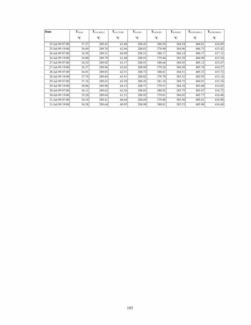
103
Date TIN,SG TG/G,SHELL TG/G,TUBE TG/G,BY TR1PH,BY TR1PH,BY TR1PH,SHELL TR1PH,SHELL
oC oC oC oC oC oC oC oC
25-Jul-99 07:00 37.27 289.43 63.48 288.43 380.54 384.54 404.81 416.0925-Jul-99 19:00 36.69 289.76 62.96 288.81 378.90 384.96 404.75 415.4226-Jul-99 07:00 34.38 289.31 60.99 288.51 380.17 386.14 406.37 417.1226-Jul-99 19:00 34.80 289.79 61.48 288.91 379.44 385.29 404.90 415.5427-Jul-99 07:00 34.52 289.92 61.17 288.91 380.64 384.92 405.12 415.6727-Jul-99 19:00 36.37 289.96 62.65 288.89 379.26 384.20 403.78 414.2728-Jul-99 07:00 36.01 289.83 62.51 288.72 380.81 384.51 405.33 415.7228-Jul-99 19:00 37.74 289.84 63.91 288.82 378.78 383.52 402.95 413.1629-Jul-99 07:00 37.16 289.63 63.39 288.43 381.18 384.75 404.91 415.3429-Jul-99 19:00 38.06 289.98 64.15 288.71 379.31 384.10 403.60 414.0230-Jul-99 07:00 36.12 289.62 62.26 288.83 380.92 385.75 405.87 416.7230-Jul-99 19:00 35.20 289.64 61.51 288.92 379.81 386.05 405.77 416.4031-Jul-99 07:00 34.10 289.41 60.64 288.69 379.88 385.50 405.81 416.9031-Jul-99 19:00 34.38 289.64 60.95 288.98 380.01 385.53 405.90 416.60

104
Table A-1 Plant Data (cont’d)
Date TR1B1 TR1B1 TR1B1 TR1B1 TR1B2 TWHBI,TUBE TWHBI,BY TR2 TWHBII,TUBE
oC oC oC oC oC oC oC oC oC
01-Feb-99 07:00 509.15 519.23 516.92 520.97 469.08 345.92 400.78 444.43 324.4201-Feb-99 19:00 509.42 519.71 517.18 521.11 469.08 345.91 400.78 444.39 324.4702-Feb-99 07:00 507.84 518.20 516.01 519.99 467.91 345.69 400.21 443.50 324.5502-Feb-99 19:00 508.81 518.80 516.49 520.29 468.78 345.78 400.53 444.06 324.4803-Feb-99 07:00 509.74 519.15 516.64 519.89 469.28 345.85 400.93 444.45 324.5303-Feb-99 19:00 508.66 518.83 516.45 520.59 468.45 345.95 400.99 444.25 324.4604-Feb-99 07:00 509.27 519.37 516.66 521.03 468.55 345.50 401.07 444.28 324.1304-Feb-99 19:00 510.70 519.86 517.36 521.07 469.90 345.77 401.93 445.35 324.3705-Feb-99 07:00 509.83 519.51 517.31 520.77 469.63 345.91 401.39 444.86 324.6105-Feb-99 19:00 509.87 519.29 517.15 520.94 468.78 345.70 401.22 444.34 324.4406-Feb-99 07:00 510.02 519.48 516.96 520.63 469.60 345.81 401.57 445.03 324.4306-Feb-99 19:00 510.11 519.95 517.72 521.82 469.75 345.92 401.34 445.03 324.5407-Feb-99 07:00 508.84 519.16 516.39 520.49 468.76 345.43 400.69 444.15 324.2907-Feb-99 19:00 507.27 518.20 515.18 520.05 467.23 345.51 399.73 442.72 324.4308-Feb-99 07:00 507.57 517.98 515.37 519.74 467.55 345.68 400.32 443.30 324.6208-Feb-99 19:00 507.42 517.86 515.33 519.62 467.35 345.50 400.21 443.30 324.3609-Feb-99 07:00 507.88 518.08 514.97 518.91 467.96 345.55 400.50 443.79 324.4409-Feb-99 19:00 507.56 517.99 515.21 519.58 467.89 345.77 400.53 443.62 324.5610-Feb-99 07:00 507.96 517.68 514.81 518.71 468.06 345.51 400.59 443.74 324.3710-Feb-99 19:00 506.90 517.82 514.71 518.99 467.00 345.52 399.92 443.09 324.4211-Feb-99 07:00 506.34 517.06 513.99 518.48 466.28 345.16 399.75 442.36 324.1411-Feb-99 19:00 505.94 516.55 513.89 518.25 466.17 345.22 399.61 442.38 324.4312-Feb-99 07:00 505.58 516.19 513.33 517.68 466.19 345.40 399.72 442.42 324.4612-Feb-99 19:00 504.88 515.33 511.54 516.17 465.83 345.20 399.76 442.14 324.3213-Feb-99 07:00 505.29 516.48 513.24 518.06 466.49 345.55 399.89 442.45 324.4113-Feb-99 19:00 505.36 516.63 513.37 518.33 466.48 345.50 399.45 442.37 324.5914-Feb-99 07:00 504.78 516.38 513.07 517.60 466.36 345.56 399.32 442.47 324.5814-Feb-99 19:00 505.25 516.28 513.02 517.12 466.20 345.49 399.39 442.41 324.6315-Feb-99 07:00 506.48 517.11 513.78 517.76 466.89 345.61 399.75 442.80 324.5715-Feb-99 19:00 505.13 516.11 512.17 516.55 466.58 345.65 399.52 442.64 324.6216-Feb-99 07:00 505.90 516.96 513.12 517.41 467.31 345.65 399.91 443.22 324.5816-Feb-99 19:00 505.59 516.70 512.85 517.23 467.12 345.73 400.06 443.13 324.7217-Feb-99 07:00 505.73 516.53 512.81 517.28 466.61 345.33 399.99 442.81 324.4217-Feb-99 19:00 506.27 516.87 513.37 517.80 467.08 345.25 400.31 442.96 324.2418-Feb-99 07:00 505.16 516.13 512.19 516.73 466.06 345.26 399.87 442.40 324.3118-Feb-99 19:00 504.74 515.63 511.73 516.26 466.05 345.18 399.70 442.32 324.2619-Feb-99 07:00 505.66 516.38 512.70 517.17 466.78 345.35 400.08 442.79 324.2619-Feb-99 19:00 505.22 516.13 512.21 516.52 466.71 345.22 399.90 442.71 324.3420-Feb-99 07:00 504.27 515.65 512.22 516.21 466.16 345.48 399.40 442.32 324.8020-Feb-99 19:00 502.47 514.45 510.48 515.06 465.03 345.54 398.82 441.58 324.7721-Feb-99 07:00 503.54 515.33 511.55 516.54 465.51 345.45 398.89 441.68 324.5621-Feb-99 19:00 505.42 516.63 512.92 517.36 466.80 345.24 399.92 442.92 324.3222-Feb-99 07:00 505.07 516.50 512.67 517.21 466.92 345.57 399.75 443.17 324.6322-Feb-99 19:00 505.36 516.77 512.77 517.03 466.66 345.49 399.67 442.68 324.5923-Feb-99 07:00 505.58 516.88 513.13 517.28 466.43 345.44 399.90 442.69 324.4326-Feb-99 19:00 505.95 517.75 514.34 518.93 465.72 344.88 398.83 443.57 319.5827-Feb-99 07:00 503.93 516.49 512.25 517.68 464.53 345.17 398.62 442.61 320.1027-Feb-99 19:00 502.74 515.10 510.72 516.16 463.53 345.17 398.32 442.12 319.9728-Feb-99 07:00 504.24 516.86 512.38 517.01 465.25 345.75 399.23 443.38 320.2228-Feb-99 19:00 503.19 515.71 511.27 516.68 464.40 344.73 398.16 442.79 319.5201-Mar-99 07:00 503.15 515.23 510.84 515.99 463.80 344.74 398.21 442.42 319.6001-Mar-99 19:00 502.71 514.76 510.05 515.33 463.33 344.76 398.18 442.11 319.49

105
Date TR1B1 TR1B1 TR1B1 TR1B1 TR1B2 TWHBI,TUBE TWHBI,BY TR2 TWHBII,TUBE
oC oC oC oC oC oC oC oC oC
02-Mar-99 07:00 503.21 515.41 511.31 516.60 463.43 344.66 398.51 442.24 319.2702-Mar-99 19:00 503.07 514.78 510.10 515.49 463.37 344.26 397.91 441.88 319.0003-Mar-99 07:00 502.06 514.10 508.98 514.45 463.22 344.01 397.86 442.01 319.0203-Mar-99 19:00 502.74 514.92 510.30 515.67 463.73 344.36 398.24 442.51 318.9004-Mar-99 07:00 502.01 515.20 510.40 515.94 463.73 344.41 398.04 442.41 319.0604-Mar-99 19:00 500.57 514.24 508.98 514.95 463.11 344.68 397.57 442.03 319.3105-Mar-99 07:00 501.00 514.69 509.73 515.30 463.33 344.72 397.87 442.28 319.2505-Mar-99 19:00 500.47 513.54 508.15 513.92 462.23 344.56 397.57 441.59 319.2806-Mar-99 07:00 502.90 515.45 510.48 515.62 464.31 345.10 398.75 443.01 319.3806-Mar-99 19:00 502.32 514.88 510.72 515.55 463.71 344.73 398.20 442.58 319.0507-Mar-99 07:00 502.04 514.58 510.92 515.53 463.14 344.20 397.90 441.77 318.8407-Mar-99 19:00 503.87 515.83 510.91 515.85 463.76 344.30 398.40 442.32 318.6008-Mar-99 07:00 501.93 514.45 508.87 514.34 463.04 344.17 397.93 442.11 318.8108-Mar-99 19:00 500.26 513.18 507.59 512.94 462.31 344.51 397.62 441.89 319.0709-Mar-99 07:00 499.71 512.72 507.10 512.45 461.78 343.95 397.63 441.54 318.6809-Mar-99 19:00 501.33 513.81 509.01 514.17 462.81 343.92 398.46 442.05 318.6010-Mar-99 07:00 504.32 516.03 511.69 516.48 464.93 344.01 399.33 443.72 318.2310-Mar-99 19:00 504.21 515.97 511.41 516.42 464.36 344.05 399.20 443.43 318.3511-Mar-99 07:00 503.66 515.73 510.93 515.90 464.23 344.00 399.15 443.25 318.3211-Mar-99 19:00 503.85 515.66 511.38 515.72 464.39 344.01 398.94 443.22 318.3812-Mar-99 07:00 503.45 515.56 510.67 515.41 464.38 344.67 399.27 443.46 318.9612-Mar-99 19:00 504.01 515.67 511.07 516.08 464.70 344.37 399.51 443.76 318.5313-Mar-99 07:00 502.25 514.48 509.45 514.86 463.46 344.37 398.87 442.97 318.9913-Mar-99 19:00 501.64 514.10 508.96 514.37 463.19 344.54 398.62 442.90 319.1914-Mar-99 07:00 500.25 513.49 508.24 513.57 462.62 344.29 398.19 442.35 318.9014-Mar-99 19:00 500.03 513.40 508.63 514.16 462.09 344.37 397.54 441.72 318.8815-Mar-99 07:00 499.26 512.54 507.57 513.92 461.81 344.27 397.44 441.45 319.1815-Mar-99 19:00 502.35 514.94 510.92 515.94 464.39 344.59 398.87 442.87 322.1216-Mar-99 07:00 502.21 514.59 509.92 514.55 464.49 344.57 398.96 442.80 322.5416-Mar-99 19:00 505.08 516.47 511.73 516.68 465.30 344.14 399.20 443.16 321.9517-Mar-99 07:00 503.20 515.74 511.34 516.29 464.73 344.41 399.31 442.83 322.4117-Mar-99 19:00 500.29 513.59 509.06 514.21 463.15 344.68 398.33 441.74 322.7118-Mar-99 07:00 500.32 513.35 508.60 513.77 463.57 344.47 398.43 441.85 322.4318-Mar-99 19:00 502.83 514.94 510.92 515.75 464.55 343.92 398.86 442.48 321.8619-Mar-99 07:00 504.51 516.69 512.87 517.20 466.33 344.35 399.65 443.77 322.1019-Mar-99 19:00 503.87 515.95 512.38 517.40 465.39 344.33 399.18 443.11 322.0920-Mar-99 07:00 503.54 516.26 512.56 517.03 465.13 344.21 398.99 442.99 322.1520-Mar-99 19:00 503.81 515.72 512.34 516.82 465.13 344.29 399.13 443.15 322.2321-Mar-99 07:00 504.00 515.84 511.88 515.90 466.02 344.69 399.60 443.62 322.4521-Mar-99 19:00 503.94 516.06 511.79 516.03 465.69 344.53 399.63 443.54 322.4122-Mar-99 07:00 503.47 515.75 511.54 515.80 465.61 344.33 399.50 443.50 322.2622-Mar-99 19:00 503.05 514.70 510.15 514.69 464.83 344.41 399.01 443.10 322.2423-Mar-99 07:00 500.87 513.76 508.47 513.45 463.72 344.57 398.64 442.42 322.6423-Mar-99 19:00 501.52 514.03 508.78 513.79 464.15 344.97 399.05 442.79 323.0424-Mar-99 07:00 501.87 514.45 509.55 514.58 464.37 345.10 399.40 442.77 323.0024-Mar-99 19:00 502.96 515.15 510.32 515.25 464.72 344.99 399.63 443.34 322.8825-Mar-99 07:00 502.46 515.06 510.33 515.36 464.58 345.09 399.59 443.13 322.9425-Mar-99 19:00 503.02 515.07 510.12 515.28 464.90 345.03 399.77 443.31 322.9926-Mar-99 07:00 501.36 514.35 508.94 513.72 464.46 345.30 399.51 443.22 323.2726-Mar-99 19:00 502.20 514.87 509.61 514.65 464.40 344.71 398.87 442.77 322.7427-Mar-99 07:00 505.85 518.59 514.22 519.34 466.53 344.57 399.61 443.57 322.2027-Mar-99 19:00 507.33 519.22 515.60 519.89 467.54 344.80 400.23 444.53 322.2928-Mar-99 07:00 506.36 517.87 514.56 518.83 467.36 345.32 400.56 444.73 322.7228-Mar-99 19:00 504.78 516.57 513.00 517.35 466.20 345.18 399.98 444.09 322.81

106
Date TR1B1 TR1B1 TR1B1 TR1B1 TR1B2 TWHBI,TUBE TWHBI,BY TR2 TWHBII,TUBE
oC oC oC oC oC oC oC oC oC
29-Mar-99 07:00 505.56 517.49 513.62 518.63 466.76 345.17 400.19 444.19 322.5229-Mar-99 19:00 506.21 517.72 514.26 518.28 467.13 345.12 400.24 444.61 322.6330-Mar-99 07:00 505.27 517.38 513.42 517.91 466.59 345.01 400.17 444.18 322.6730-Mar-99 19:00 502.87 515.64 511.11 515.72 464.64 344.85 398.92 442.96 322.7831-Mar-99 07:00 502.39 514.70 509.56 514.32 464.63 345.18 399.27 442.91 322.8431-Mar-99 19:00 503.39 515.11 510.24 514.77 465.47 345.38 399.78 443.55 323.1101-Jul-99 07:00 506.62 518.25 513.52 517.65 468.59 345.58 398.49 442.47 327.3501-Jul-99 19:00 502.38 516.04 510.68 515.12 466.42 345.39 397.37 440.59 327.4702-Jul-99 07:00 504.44 518.07 512.81 516.80 467.70 345.38 397.89 441.21 327.4002-Jul-99 19:00 502.84 516.26 510.26 514.77 466.09 345.11 397.01 440.36 327.4503-Jul-99 07:00 506.12 517.72 512.07 516.56 467.87 345.15 397.96 441.45 327.1503-Jul-99 19:00 503.60 516.77 510.45 515.51 466.61 345.15 397.20 440.54 327.2504-Jul-99 07:00 505.67 518.24 512.20 516.92 467.62 345.30 397.87 440.92 327.0504-Jul-99 19:00 505.58 518.17 513.26 517.46 467.55 345.18 397.72 440.88 327.1805-Jul-99 07:00 504.56 518.14 512.50 517.15 466.86 345.35 397.66 440.32 327.2805-Jul-99 19:00 504.47 517.99 511.98 516.66 467.18 345.07 397.16 441.06 327.0006-Jul-99 07:00 500.56 514.68 509.37 514.48 465.26 345.07 396.59 439.91 327.6006-Jul-99 19:00 499.58 514.38 508.65 513.40 464.47 345.03 396.30 439.66 327.3907-Jul-99 07:00 502.16 515.95 509.94 514.41 466.13 345.35 397.26 440.35 327.6807-Jul-99 19:00 499.01 513.82 506.77 512.16 464.51 345.03 396.42 439.72 327.5608-Jul-99 07:00 498.63 513.28 506.51 512.38 464.34 344.91 396.21 439.71 327.2108-Jul-99 19:00 503.69 516.60 511.58 516.51 466.62 345.05 397.14 440.62 327.2509-Jul-99 07:00 501.25 514.68 508.94 513.67 465.33 345.24 396.93 439.91 327.4209-Jul-99 19:00 502.70 516.10 510.61 514.90 466.24 345.35 396.99 440.85 327.3710-Jul-99 07:00 503.95 516.80 512.51 516.54 467.00 345.31 397.81 441.02 327.4810-Jul-99 19:00 500.20 514.67 509.40 514.71 465.13 345.24 396.36 439.74 327.2111-Jul-99 07:00 502.76 516.92 511.94 517.09 466.59 345.33 397.38 440.56 327.2811-Jul-99 19:00 496.52 512.71 506.09 511.98 463.26 344.69 395.06 438.36 327.0812-Jul-99 07:00 500.58 514.93 508.31 513.39 465.65 344.99 396.36 440.07 327.1412-Jul-99 19:00 503.20 516.51 510.69 515.05 466.75 344.99 396.91 441.13 326.8313-Jul-99 07:00 503.96 516.92 510.62 514.92 467.38 345.29 397.09 441.43 327.1713-Jul-99 19:00 502.64 516.19 510.80 515.07 466.31 345.03 396.97 440.53 327.2214-Jul-99 07:00 502.29 515.99 511.26 515.46 466.40 345.11 397.13 440.65 327.2914-Jul-99 19:00 500.27 514.30 508.12 512.42 464.95 345.07 396.08 439.70 327.3315-Jul-99 07:00 500.12 514.97 508.16 513.02 464.88 344.87 396.02 439.45 327.0215-Jul-99 19:00 503.15 514.41 509.45 512.90 464.97 341.85 394.48 438.67 327.4216-Jul-99 07:00 504.15 512.58 510.78 513.35 464.30 337.89 392.21 436.34 328.0216-Jul-99 19:00 504.18 512.79 510.42 513.41 465.02 339.01 392.90 437.23 329.2317-Jul-99 07:00 509.07 518.35 516.27 518.66 469.24 342.92 397.19 442.31 326.6417-Jul-99 19:00 507.30 517.66 514.14 517.28 467.75 343.76 396.93 441.89 325.5518-Jul-99 07:00 503.40 516.17 510.13 514.75 465.97 344.48 396.68 440.38 326.6718-Jul-99 19:00 499.69 514.36 506.94 512.04 464.64 344.29 396.03 439.37 326.6619-Jul-99 07:00 503.42 516.72 511.33 515.81 466.89 344.91 397.52 441.36 326.9419-Jul-99 19:00 501.50 515.34 509.54 515.26 465.62 344.67 396.70 440.42 327.2920-Jul-99 07:00 504.00 517.34 512.07 516.53 467.43 344.97 397.97 441.43 327.3120-Jul-99 19:00 500.75 514.99 508.68 513.55 465.39 344.87 396.53 440.45 327.2021-Jul-99 07:00 501.66 516.05 509.63 514.88 466.21 344.76 396.72 440.88 326.7221-Jul-99 19:00 504.30 517.02 511.22 515.56 467.41 344.43 397.12 441.70 326.5722-Jul-99 07:00 501.76 515.83 509.31 514.08 466.01 344.72 396.68 440.70 326.8122-Jul-99 19:00 503.71 516.82 510.48 515.94 467.09 344.21 396.53 441.37 326.0523-Jul-99 07:00 503.36 516.90 511.33 516.50 466.99 344.67 397.19 441.31 326.8123-Jul-99 19:00 500.58 514.70 508.21 513.32 465.33 344.66 396.22 440.46 326.9324-Jul-99 07:00 503.69 515.61 509.76 513.65 464.91 342.95 395.35 439.73 324.9024-Jul-99 19:00 500.79 514.53 506.71 511.89 465.13 343.90 395.93 440.34 326.45

107
Date TR1B1 TR1B1 TR1B1 TR1B1 TR1B2 TWHBI,TUBE TWHBI,BY TR2 TWHBII,TUBE
oC oC oC oC oC oC oC oC oC
25-Jul-99 07:00 504.85 517.32 512.37 516.33 467.87 344.25 397.12 442.16 326.1925-Jul-99 19:00 504.07 517.51 511.49 516.45 467.39 344.68 397.11 441.54 326.6326-Jul-99 07:00 508.20 519.58 515.69 519.47 469.30 344.76 398.71 442.89 326.7426-Jul-99 19:00 503.04 516.71 511.78 516.36 466.43 344.80 396.99 440.90 327.1927-Jul-99 07:00 502.82 516.41 511.50 515.96 466.58 344.84 397.51 440.90 327.2127-Jul-99 19:00 500.23 514.57 508.96 514.04 464.80 344.36 396.30 439.95 326.6428-Jul-99 07:00 503.79 517.16 511.27 515.59 467.01 344.83 397.33 441.13 326.8328-Jul-99 19:00 499.07 513.63 506.47 511.63 463.83 344.06 395.47 439.59 326.5229-Jul-99 07:00 503.77 517.19 511.27 515.33 467.24 344.46 397.05 441.50 326.5329-Jul-99 19:00 501.11 515.30 508.44 513.90 465.61 344.21 396.55 440.90 326.4930-Jul-99 07:00 506.60 519.35 514.05 517.89 468.65 344.26 398.57 442.63 326.6630-Jul-99 19:00 506.25 519.10 513.47 517.98 468.01 344.42 398.41 442.14 326.6231-Jul-99 07:00 506.89 519.33 514.25 518.97 468.37 344.44 398.88 442.43 326.7931-Jul-99 19:00 505.89 519.15 513.77 518.01 467.75 344.43 398.38 441.87 326.84

108
Table A-1 Plant Data (cont’d)
Date MNH3,RECVR,1 MNH3,RECVR,2 HVG/G,SHELL HVR1PH,TUBE HVWHBI,TUBE HVWHBII,STEAM LWHBII LVWHBII
tonne/hr m3/hr % % % % % %
01-Feb-99 07:00 76.71 1.70 0.00 0.00 84.00 5.00 61.03 75.3501-Feb-99 19:00 76.72 1.55 0.00 0.00 84.00 5.00 60.96 74.8102-Feb-99 07:00 76.73 1.76 0.00 0.00 84.00 5.00 61.02 74.6402-Feb-99 19:00 76.72 1.74 0.00 0.00 84.00 5.00 60.99 74.9603-Feb-99 07:00 76.74 1.65 0.00 0.00 84.00 5.00 61.13 74.6403-Feb-99 19:00 76.76 1.81 0.00 0.00 84.00 5.00 60.98 72.6404-Feb-99 07:00 76.22 1.87 0.00 0.00 84.00 5.00 61.00 73.7704-Feb-99 19:00 76.86 1.73 0.00 0.00 85.53 5.00 61.01 75.8905-Feb-99 07:00 77.05 1.42 0.00 0.00 87.00 5.00 61.05 75.2205-Feb-99 19:00 77.05 1.71 0.00 0.00 87.00 5.00 61.02 74.8006-Feb-99 07:00 77.08 1.72 0.00 0.00 87.00 5.00 61.25 74.6106-Feb-99 19:00 76.94 1.87 0.00 0.00 87.00 5.00 60.97 75.2407-Feb-99 07:00 76.89 1.95 0.00 0.00 87.00 5.00 61.09 74.7707-Feb-99 19:00 76.77 1.68 0.00 0.00 87.00 5.00 61.01 75.5408-Feb-99 07:00 76.80 1.70 0.00 0.00 87.00 5.00 61.06 75.6708-Feb-99 19:00 76.58 1.94 0.00 0.00 87.00 5.00 61.04 74.6709-Feb-99 07:00 76.90 1.75 0.00 0.00 87.00 5.00 60.98 74.8909-Feb-99 19:00 76.93 1.63 0.00 0.00 87.00 5.00 60.98 75.6610-Feb-99 07:00 76.75 1.77 0.00 0.00 87.00 5.00 61.06 75.7310-Feb-99 19:00 76.57 1.36 0.00 0.00 87.00 5.00 61.05 74.1611-Feb-99 07:00 76.52 1.49 0.00 0.00 87.00 5.00 60.96 74.3711-Feb-99 19:00 76.67 1.83 0.00 0.00 87.00 5.00 60.94 74.6212-Feb-99 07:00 76.91 1.68 0.00 0.00 87.00 5.00 60.99 74.4312-Feb-99 19:00 76.97 1.90 0.00 0.00 87.00 5.00 61.01 75.1413-Feb-99 07:00 76.85 1.77 0.00 0.00 87.00 5.00 61.03 75.7613-Feb-99 19:00 76.49 1.82 0.00 0.00 87.00 5.00 60.99 75.6014-Feb-99 07:00 76.45 1.88 0.00 0.00 87.00 5.00 61.07 75.1214-Feb-99 19:00 76.43 1.57 0.00 0.00 87.00 5.00 61.01 75.2615-Feb-99 07:00 76.43 1.88 0.00 0.00 87.00 5.00 61.04 75.1215-Feb-99 19:00 76.62 1.79 0.00 0.00 87.00 5.00 60.96 74.9816-Feb-99 07:00 76.61 1.77 0.00 0.00 87.00 5.00 61.02 75.3516-Feb-99 19:00 76.68 1.73 0.00 0.00 87.00 5.00 61.02 75.1817-Feb-99 07:00 76.53 1.75 0.00 0.00 87.00 5.00 61.01 74.6717-Feb-99 19:00 76.66 1.70 0.00 0.00 87.00 5.00 60.90 75.1018-Feb-99 07:00 76.58 1.43 0.00 0.00 87.00 5.00 61.06 75.1618-Feb-99 19:00 76.47 1.74 0.00 0.00 87.00 5.00 61.07 74.8919-Feb-99 07:00 76.55 1.02 0.00 0.00 87.00 5.00 61.01 75.1719-Feb-99 19:00 76.58 1.17 0.00 0.00 87.00 5.00 61.00 75.3920-Feb-99 07:00 76.72 1.92 0.00 0.00 87.00 5.00 61.00 75.7420-Feb-99 19:00 76.59 2.22 0.00 0.00 87.00 5.00 61.04 75.4621-Feb-99 07:00 76.37 1.70 0.00 0.00 87.00 5.00 61.02 75.0321-Feb-99 19:00 76.64 2.11 0.00 0.00 87.00 5.00 61.02 75.5922-Feb-99 07:00 76.61 1.46 0.00 0.00 87.00 5.00 61.03 76.0922-Feb-99 19:00 76.58 1.23 0.00 0.00 87.00 5.00 61.08 75.6523-Feb-99 07:00 76.23 2.40 0.00 0.00 87.00 5.00 61.07 74.8226-Feb-99 19:00 75.67 1.48 0.00 0.00 86.00 5.00 61.35 73.9727-Feb-99 07:00 77.21 1.48 0.00 0.00 86.00 5.00 60.00 75.3227-Feb-99 19:00 77.24 2.12 0.00 0.00 87.99 5.00 60.04 75.2628-Feb-99 07:00 77.46 1.56 0.00 0.00 88.00 5.00 59.99 74.9028-Feb-99 19:00 77.45 2.17 0.00 0.00 88.00 5.00 59.99 76.1001-Mar-99 07:00 77.50 2.03 0.00 0.00 88.00 5.00 60.02 77.3101-Mar-99 19:00 77.48 2.30 0.00 0.00 88.00 5.00 60.06 77.11

109
Date MNH3,RECVR,1 MNH3,RECVR,2 HVG/G,SHELL HVR1PH,TUBE HVWHBI,TUBE HVWHBII,STEAM LWHBII LVWHBII
tonne/hr m3/hr % % % % % %
02-Mar-99 07:00 77.60 1.93 0.00 0.00 88.00 5.00 60.06 76.3102-Mar-99 19:00 77.67 1.48 0.00 0.00 88.00 5.00 60.03 75.4003-Mar-99 07:00 77.64 1.87 0.00 0.00 88.00 5.00 60.05 75.6203-Mar-99 19:00 77.52 1.86 0.00 0.00 88.00 5.00 60.07 75.8704-Mar-99 07:00 77.47 1.46 0.00 0.00 88.00 5.00 60.05 75.7704-Mar-99 19:00 77.50 2.17 0.00 0.00 88.00 5.00 60.01 76.0505-Mar-99 07:00 77.52 1.67 0.00 0.00 88.00 5.00 60.04 76.0305-Mar-99 19:00 77.55 1.72 0.00 0.00 88.00 5.00 59.97 76.1506-Mar-99 07:00 77.72 2.05 0.00 0.00 88.00 5.00 60.04 76.5406-Mar-99 19:00 77.58 2.49 0.00 0.00 89.81 5.00 60.07 76.5807-Mar-99 07:00 77.68 1.54 0.00 0.00 90.00 5.00 60.02 76.0507-Mar-99 19:00 77.62 2.19 0.00 0.00 90.00 5.00 60.04 76.4208-Mar-99 07:00 77.25 1.09 0.00 0.00 91.81 5.00 60.05 76.5608-Mar-99 19:00 77.12 2.37 0.00 0.00 94.00 5.00 60.05 76.5509-Mar-99 07:00 77.14 1.76 0.00 0.00 94.00 5.00 60.00 76.4909-Mar-99 19:00 77.26 2.17 0.00 0.00 94.00 5.00 60.02 76.6010-Mar-99 07:00 77.51 2.31 0.00 0.00 94.00 5.00 60.07 76.8910-Mar-99 19:00 77.52 1.70 0.00 0.00 94.00 5.00 60.03 76.9711-Mar-99 07:00 77.57 1.79 0.00 0.00 94.00 5.00 60.05 76.5711-Mar-99 19:00 77.12 1.55 0.00 0.00 94.00 5.00 61.46 76.0112-Mar-99 07:00 77.59 2.22 0.00 0.00 94.00 5.00 62.98 75.9112-Mar-99 19:00 77.56 1.61 0.00 0.00 94.00 5.00 62.98 77.1213-Mar-99 07:00 77.64 1.33 0.00 0.00 94.00 5.00 62.01 77.0113-Mar-99 19:00 77.45 1.10 0.00 0.00 94.00 5.00 61.98 77.1414-Mar-99 07:00 77.47 2.09 0.00 0.00 94.00 5.00 62.00 77.0514-Mar-99 19:00 77.19 1.96 0.00 0.00 94.00 5.00 61.99 77.2515-Mar-99 07:00 77.33 2.20 0.00 0.00 94.00 5.00 62.02 77.5215-Mar-99 19:00 77.16 1.57 0.00 0.00 94.00 5.00 62.06 76.3416-Mar-99 07:00 77.25 2.12 0.00 0.00 94.00 5.00 62.00 76.3416-Mar-99 19:00 76.09 1.84 0.00 0.00 94.00 5.00 62.02 75.0517-Mar-99 07:00 77.30 2.32 0.00 0.00 94.00 5.00 61.98 76.3917-Mar-99 19:00 77.27 2.31 0.00 0.00 94.00 5.00 62.00 76.4218-Mar-99 07:00 77.27 1.93 0.00 0.00 94.00 5.00 62.08 75.8818-Mar-99 19:00 77.28 2.05 0.00 0.00 94.00 5.00 61.99 75.3319-Mar-99 07:00 77.33 2.22 0.00 0.00 94.00 5.00 62.00 75.9519-Mar-99 19:00 77.11 2.23 0.00 0.00 94.00 5.00 62.01 75.8820-Mar-99 07:00 77.25 1.31 0.00 0.00 94.00 5.00 62.04 75.5020-Mar-99 19:00 77.27 1.81 0.00 0.00 94.00 5.00 61.99 76.1421-Mar-99 07:00 77.33 1.86 0.00 0.00 94.00 5.00 62.04 76.3421-Mar-99 19:00 77.39 2.36 0.00 0.00 94.00 5.00 61.98 76.3922-Mar-99 07:00 77.51 2.12 0.00 0.00 94.00 5.00 62.05 75.9922-Mar-99 19:00 77.47 2.24 0.00 0.00 94.00 5.00 62.01 76.3923-Mar-99 07:00 77.36 2.20 0.00 0.00 94.00 5.00 61.96 76.7223-Mar-99 19:00 77.26 1.84 0.00 0.00 94.00 5.00 61.95 78.0124-Mar-99 07:00 77.45 1.61 0.00 0.00 94.00 5.00 62.02 77.4924-Mar-99 19:00 77.34 1.91 0.00 0.00 94.00 5.00 61.97 77.6325-Mar-99 07:00 77.36 1.63 0.00 0.00 94.00 5.00 62.02 77.5925-Mar-99 19:00 77.31 1.82 0.00 0.00 94.00 5.00 61.98 78.4126-Mar-99 07:00 77.38 1.33 0.00 0.00 94.00 5.00 62.08 76.6826-Mar-99 19:00 77.04 2.20 0.00 0.00 94.00 5.00 61.98 76.5327-Mar-99 07:00 76.99 2.21 0.00 0.00 94.00 5.00 62.03 77.6227-Mar-99 19:00 76.97 1.42 0.00 0.00 94.00 5.00 61.98 78.3828-Mar-99 07:00 77.18 1.49 0.00 0.00 94.00 5.00 62.00 78.9728-Mar-99 19:00 77.05 1.99 0.00 0.00 94.00 5.00 61.98 78.99
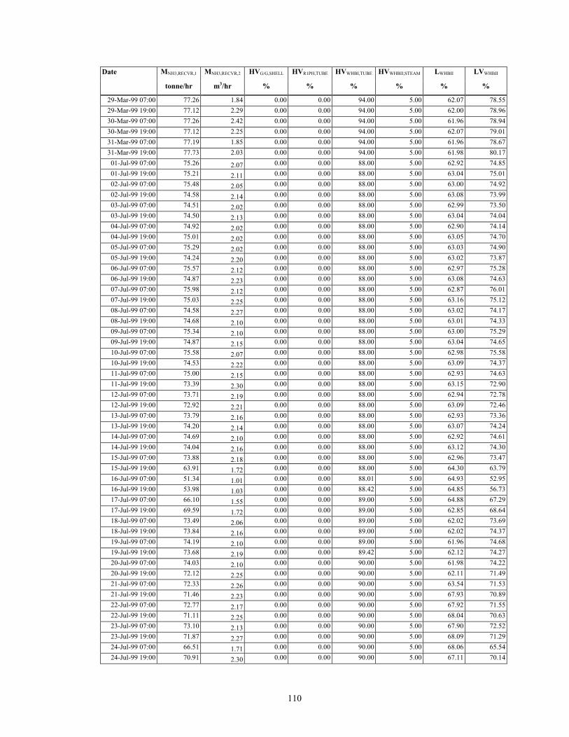
110
Date MNH3,RECVR,1 MNH3,RECVR,2 HVG/G,SHELL HVR1PH,TUBE HVWHBI,TUBE HVWHBII,STEAM LWHBII LVWHBII
tonne/hr m3/hr % % % % % %
29-Mar-99 07:00 77.26 1.84 0.00 0.00 94.00 5.00 62.07 78.5529-Mar-99 19:00 77.12 2.29 0.00 0.00 94.00 5.00 62.00 78.9630-Mar-99 07:00 77.26 2.42 0.00 0.00 94.00 5.00 61.96 78.9430-Mar-99 19:00 77.12 2.25 0.00 0.00 94.00 5.00 62.07 79.0131-Mar-99 07:00 77.19 1.85 0.00 0.00 94.00 5.00 61.96 78.6731-Mar-99 19:00 77.73 2.03 0.00 0.00 94.00 5.00 61.98 80.1701-Jul-99 07:00 75.26 2.07 0.00 0.00 88.00 5.00 62.92 74.8501-Jul-99 19:00 75.21 2.11 0.00 0.00 88.00 5.00 63.04 75.0102-Jul-99 07:00 75.48 2.05 0.00 0.00 88.00 5.00 63.00 74.9202-Jul-99 19:00 74.58 2.14 0.00 0.00 88.00 5.00 63.08 73.9903-Jul-99 07:00 74.51 2.02 0.00 0.00 88.00 5.00 62.99 73.5003-Jul-99 19:00 74.50 2.13 0.00 0.00 88.00 5.00 63.04 74.0404-Jul-99 07:00 74.92 2.02 0.00 0.00 88.00 5.00 62.90 74.1404-Jul-99 19:00 75.01 2.02 0.00 0.00 88.00 5.00 63.05 74.7005-Jul-99 07:00 75.29 2.02 0.00 0.00 88.00 5.00 63.03 74.9005-Jul-99 19:00 74.24 2.20 0.00 0.00 88.00 5.00 63.02 73.8706-Jul-99 07:00 75.57 2.12 0.00 0.00 88.00 5.00 62.97 75.2806-Jul-99 19:00 74.87 2.23 0.00 0.00 88.00 5.00 63.08 74.6307-Jul-99 07:00 75.98 2.12 0.00 0.00 88.00 5.00 62.87 76.0107-Jul-99 19:00 75.03 2.25 0.00 0.00 88.00 5.00 63.16 75.1208-Jul-99 07:00 74.58 2.27 0.00 0.00 88.00 5.00 63.02 74.1708-Jul-99 19:00 74.68 2.10 0.00 0.00 88.00 5.00 63.01 74.3309-Jul-99 07:00 75.34 2.10 0.00 0.00 88.00 5.00 63.00 75.2909-Jul-99 19:00 74.87 2.15 0.00 0.00 88.00 5.00 63.04 74.6510-Jul-99 07:00 75.58 2.07 0.00 0.00 88.00 5.00 62.98 75.5810-Jul-99 19:00 74.53 2.22 0.00 0.00 88.00 5.00 63.09 74.3711-Jul-99 07:00 75.00 2.15 0.00 0.00 88.00 5.00 62.93 74.6311-Jul-99 19:00 73.39 2.30 0.00 0.00 88.00 5.00 63.15 72.9012-Jul-99 07:00 73.71 2.19 0.00 0.00 88.00 5.00 62.94 72.7812-Jul-99 19:00 72.92 2.21 0.00 0.00 88.00 5.00 63.09 72.4613-Jul-99 07:00 73.79 2.16 0.00 0.00 88.00 5.00 62.93 73.3613-Jul-99 19:00 74.20 2.14 0.00 0.00 88.00 5.00 63.07 74.2414-Jul-99 07:00 74.69 2.10 0.00 0.00 88.00 5.00 62.92 74.6114-Jul-99 19:00 74.04 2.16 0.00 0.00 88.00 5.00 63.12 74.3015-Jul-99 07:00 73.88 2.18 0.00 0.00 88.00 5.00 62.96 73.4715-Jul-99 19:00 63.91 1.72 0.00 0.00 88.00 5.00 64.30 63.7916-Jul-99 07:00 51.34 1.01 0.00 0.00 88.01 5.00 64.93 52.9516-Jul-99 19:00 53.98 1.03 0.00 0.00 88.42 5.00 64.85 56.7317-Jul-99 07:00 66.10 1.55 0.00 0.00 89.00 5.00 64.88 67.2917-Jul-99 19:00 69.59 1.72 0.00 0.00 89.00 5.00 62.85 68.6418-Jul-99 07:00 73.49 2.06 0.00 0.00 89.00 5.00 62.02 73.6918-Jul-99 19:00 73.84 2.16 0.00 0.00 89.00 5.00 62.02 74.3719-Jul-99 07:00 74.19 2.10 0.00 0.00 89.00 5.00 61.96 74.6819-Jul-99 19:00 73.68 2.19 0.00 0.00 89.42 5.00 62.12 74.2720-Jul-99 07:00 74.03 2.10 0.00 0.00 90.00 5.00 61.98 74.2220-Jul-99 19:00 72.12 2.25 0.00 0.00 90.00 5.00 62.11 71.4921-Jul-99 07:00 72.33 2.26 0.00 0.00 90.00 5.00 63.54 71.5321-Jul-99 19:00 71.46 2.23 0.00 0.00 90.00 5.00 67.93 70.8922-Jul-99 07:00 72.77 2.17 0.00 0.00 90.00 5.00 67.92 71.5522-Jul-99 19:00 71.11 2.25 0.00 0.00 90.00 5.00 68.04 70.6323-Jul-99 07:00 73.10 2.13 0.00 0.00 90.00 5.00 67.90 72.5223-Jul-99 19:00 71.87 2.27 0.00 0.00 90.00 5.00 68.09 71.2924-Jul-99 07:00 66.51 1.71 0.00 0.00 90.00 5.00 68.06 65.5424-Jul-99 19:00 70.91 2.30 0.00 0.00 90.00 5.00 67.11 70.14

111
Date MNH3,RECVR,1 MNH3,RECVR,2 HVG/G,SHELL HVR1PH,TUBE HVWHBI,TUBE HVWHBII,STEAM LWHBII LVWHBII
tonne/hr m3/hr % % % % % %
25-Jul-99 07:00 72.03 2.25 0.00 0.00 90.00 5.00 66.91 71.5625-Jul-99 19:00 73.01 2.19 0.00 0.00 90.00 5.00 66.98 72.7126-Jul-99 07:00 74.63 1.94 0.00 0.00 90.00 5.00 66.89 74.5326-Jul-99 19:00 74.10 2.09 0.00 0.00 90.00 5.00 67.04 74.3527-Jul-99 07:00 74.58 2.05 0.00 0.00 90.00 5.00 66.90 74.7127-Jul-99 19:00 72.71 2.23 0.00 0.00 90.00 5.00 64.44 73.1028-Jul-99 07:00 73.11 2.17 0.00 0.00 90.00 5.00 62.96 73.0128-Jul-99 19:00 71.26 2.37 0.00 0.00 90.00 5.00 63.13 71.2529-Jul-99 07:00 71.82 2.28 0.00 0.00 90.00 5.00 62.94 71.2929-Jul-99 19:00 70.80 2.40 0.00 0.00 91.68 5.00 63.09 70.7130-Jul-99 07:00 72.91 2.20 0.00 0.00 92.00 5.00 62.92 72.7530-Jul-99 19:00 73.62 2.14 0.00 0.00 92.00 5.00 63.03 73.5631-Jul-99 07:00 74.88 2.01 0.00 0.00 92.00 5.00 62.88 74.6531-Jul-99 19:00 75.07 2.08 0.00 0.00 92.00 5.00 63.05 75.89
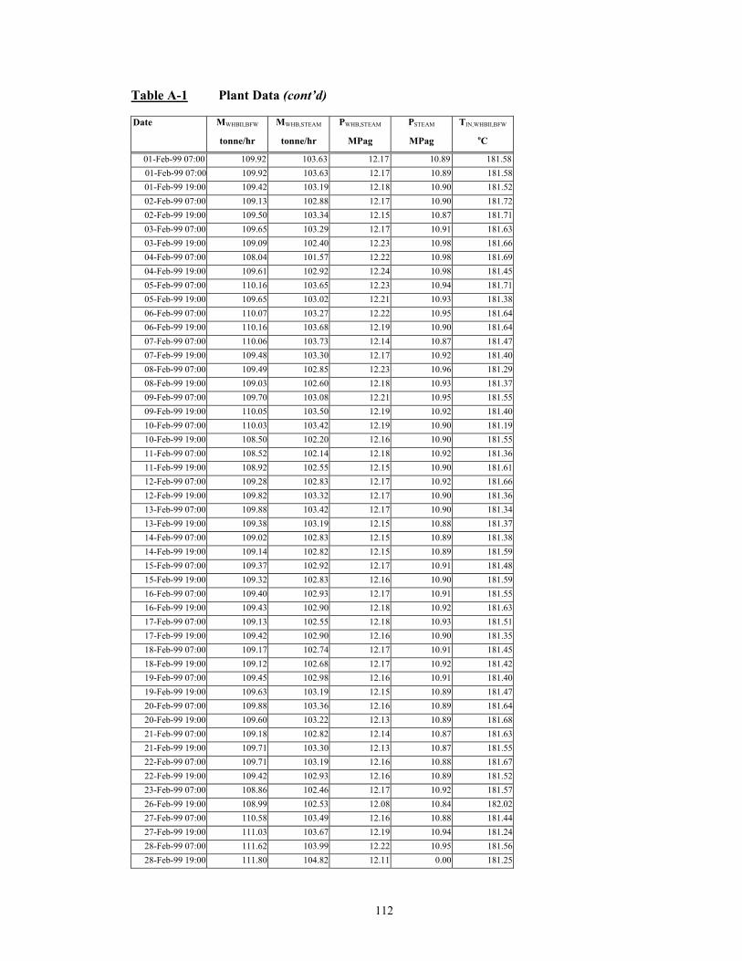
112
Table A-1 Plant Data (cont’d)
Date MWHBII,BFW MWHB,STEAM PWHB,STEAM PSTEAM TIN,WHBII,BFW
tonne/hr tonne/hr MPag MPag oC
01-Feb-99 07:00 109.92 103.63 12.17 10.89 181.5801-Feb-99 07:00 109.92 103.63 12.17 10.89 181.5801-Feb-99 19:00 109.42 103.19 12.18 10.90 181.5202-Feb-99 07:00 109.13 102.88 12.17 10.90 181.7202-Feb-99 19:00 109.50 103.34 12.15 10.87 181.7103-Feb-99 07:00 109.65 103.29 12.17 10.91 181.6303-Feb-99 19:00 109.09 102.40 12.23 10.98 181.6604-Feb-99 07:00 108.04 101.57 12.22 10.98 181.6904-Feb-99 19:00 109.61 102.92 12.24 10.98 181.4505-Feb-99 07:00 110.16 103.65 12.23 10.94 181.7105-Feb-99 19:00 109.65 103.02 12.21 10.93 181.3806-Feb-99 07:00 110.07 103.27 12.22 10.95 181.6406-Feb-99 19:00 110.16 103.68 12.19 10.90 181.6407-Feb-99 07:00 110.06 103.73 12.14 10.87 181.4707-Feb-99 19:00 109.48 103.30 12.17 10.92 181.4008-Feb-99 07:00 109.49 102.85 12.23 10.96 181.2908-Feb-99 19:00 109.03 102.60 12.18 10.93 181.3709-Feb-99 07:00 109.70 103.08 12.21 10.95 181.5509-Feb-99 19:00 110.05 103.50 12.19 10.92 181.4010-Feb-99 07:00 110.03 103.42 12.19 10.90 181.1910-Feb-99 19:00 108.50 102.20 12.16 10.90 181.5511-Feb-99 07:00 108.52 102.14 12.18 10.92 181.3611-Feb-99 19:00 108.92 102.55 12.15 10.90 181.6112-Feb-99 07:00 109.28 102.83 12.17 10.92 181.6612-Feb-99 19:00 109.82 103.32 12.17 10.90 181.3613-Feb-99 07:00 109.88 103.42 12.17 10.90 181.3413-Feb-99 19:00 109.38 103.19 12.15 10.88 181.3714-Feb-99 07:00 109.02 102.83 12.15 10.89 181.3814-Feb-99 19:00 109.14 102.82 12.15 10.89 181.5915-Feb-99 07:00 109.37 102.92 12.17 10.91 181.4815-Feb-99 19:00 109.32 102.83 12.16 10.90 181.5916-Feb-99 07:00 109.40 102.93 12.17 10.91 181.5516-Feb-99 19:00 109.43 102.90 12.18 10.92 181.6317-Feb-99 07:00 109.13 102.55 12.18 10.93 181.5117-Feb-99 19:00 109.42 102.90 12.16 10.90 181.3518-Feb-99 07:00 109.17 102.74 12.17 10.91 181.4518-Feb-99 19:00 109.12 102.68 12.17 10.92 181.4219-Feb-99 07:00 109.45 102.98 12.16 10.91 181.4019-Feb-99 19:00 109.63 103.19 12.15 10.89 181.4720-Feb-99 07:00 109.88 103.36 12.16 10.89 181.6420-Feb-99 19:00 109.60 103.22 12.13 10.89 181.6821-Feb-99 07:00 109.18 102.82 12.14 10.87 181.6321-Feb-99 19:00 109.71 103.30 12.13 10.87 181.5522-Feb-99 07:00 109.71 103.19 12.16 10.88 181.6722-Feb-99 19:00 109.42 102.93 12.16 10.89 181.5223-Feb-99 07:00 108.86 102.46 12.17 10.92 181.5726-Feb-99 19:00 108.99 102.53 12.08 10.84 182.0227-Feb-99 07:00 110.58 103.49 12.16 10.88 181.4427-Feb-99 19:00 111.03 103.67 12.19 10.94 181.2428-Feb-99 07:00 111.62 103.99 12.22 10.95 181.5628-Feb-99 19:00 111.80 104.82 12.11 0.00 181.25
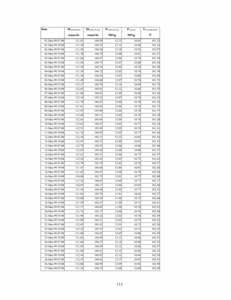
113
Date MWHBII,BFW MWHB,STEAM PWHB,STEAM PSTEAM TIN,WHBII,BFW
tonne/hr tonne/hr MPag MPag oC
01-Mar-99 07:00 111.63 104.50 12.13 10.85 181.3301-Mar-99 19:00 111.50 104.25 12.15 10.88 181.1402-Mar-99 07:00 111.58 104.24 12.18 10.92 181.0702-Mar-99 19:00 111.70 104.79 12.09 10.81 181.2703-Mar-99 07:00 111.66 104.87 12.06 10.79 181.3903-Mar-99 19:00 111.56 104.73 12.07 10.80 181.3604-Mar-99 07:00 111.36 104.76 12.05 10.78 181.5004-Mar-99 19:00 111.36 104.72 12.05 10.76 181.7005-Mar-99 07:00 111.30 104.56 12.07 10.80 181.6905-Mar-99 19:00 111.49 104.68 12.07 10.78 181.7306-Mar-99 07:00 112.17 104.79 12.16 10.90 181.7506-Mar-99 19:00 112.03 104.81 12.12 10.86 181.5507-Mar-99 07:00 111.86 104.83 12.09 10.80 181.5607-Mar-99 19:00 112.14 105.23 12.07 10.79 181.3308-Mar-99 07:00 111.78 104.87 12.06 10.78 181.3408-Mar-99 19:00 111.81 104.85 12.06 10.78 181.7309-Mar-99 07:00 111.93 105.00 12.04 10.78 181.3709-Mar-99 19:00 112.06 105.11 12.05 10.78 181.2910-Mar-99 07:00 112.63 105.66 12.04 10.76 181.2010-Mar-99 19:00 112.63 105.67 12.03 10.77 181.2411-Mar-99 07:00 112.51 105.45 12.05 10.78 181.3111-Mar-99 19:00 111.76 104.82 12.05 10.77 181.4412-Mar-99 07:00 112.54 105.11 12.12 10.85 181.5412-Mar-99 19:00 112.97 105.72 12.09 10.83 181.2313-Mar-99 07:00 112.79 105.55 12.08 10.80 181.4013-Mar-99 19:00 112.65 105.42 12.08 10.80 181.5714-Mar-99 07:00 112.61 105.51 12.06 10.77 181.4714-Mar-99 19:00 112.26 105.43 12.03 10.75 181.6315-Mar-99 07:00 112.79 105.76 12.03 10.76 182.2715-Mar-99 19:00 111.47 104.68 12.06 10.81 182.2616-Mar-99 07:00 111.65 104.91 12.04 10.78 182.3416-Mar-99 19:00 110.08 103.75 12.01 10.77 182.4017-Mar-99 07:00 111.36 104.65 12.04 10.77 182.1717-Mar-99 19:00 110.95 104.17 12.06 10.82 182.2018-Mar-99 07:00 111.36 104.69 12.02 10.77 182.3218-Mar-99 19:00 111.83 105.79 11.91 10.65 182.2719-Mar-99 07:00 112.00 105.54 11.98 10.72 182.4019-Mar-99 19:00 111.59 105.27 11.98 10.71 182.4120-Mar-99 07:00 111.17 104.89 11.98 10.70 182.5320-Mar-99 19:00 111.74 105.17 12.00 10.74 182.4021-Mar-99 07:00 111.96 105.22 12.02 10.76 182.3921-Mar-99 19:00 111.99 105.31 12.03 10.75 182.2222-Mar-99 07:00 112.05 105.42 12.01 10.73 182.2022-Mar-99 19:00 112.25 105.55 12.01 10.73 182.2223-Mar-99 07:00 111.80 104.82 12.05 10.80 182.2923-Mar-99 19:00 111.82 104.49 12.12 10.86 182.2324-Mar-99 07:00 111.66 104.27 12.14 10.88 182.3224-Mar-99 19:00 111.83 104.59 12.12 10.86 182.2725-Mar-99 07:00 111.84 104.61 12.12 10.86 182.2325-Mar-99 19:00 112.16 104.92 12.12 10.84 182.2426-Mar-99 07:00 112.53 104.92 12.17 10.92 182.5126-Mar-99 19:00 112.06 104.99 12.09 10.86 182.5027-Mar-99 07:00 111.24 104.72 12.04 10.80 182.49
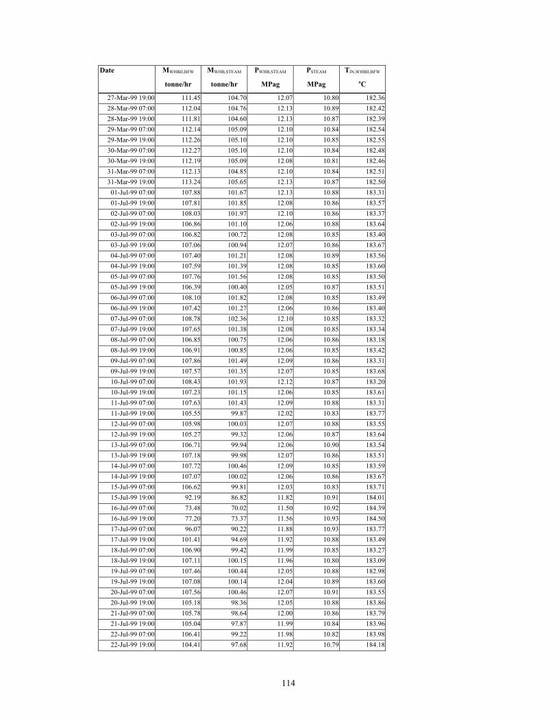
114
Date MWHBII,BFW MWHB,STEAM PWHB,STEAM PSTEAM TIN,WHBII,BFW
tonne/hr tonne/hr MPag MPag oC
27-Mar-99 19:00 111.45 104.70 12.07 10.80 182.3628-Mar-99 07:00 112.04 104.76 12.13 10.89 182.4228-Mar-99 19:00 111.81 104.60 12.13 10.87 182.3929-Mar-99 07:00 112.14 105.09 12.10 10.84 182.5429-Mar-99 19:00 112.26 105.10 12.10 10.85 182.5530-Mar-99 07:00 112.27 105.10 12.10 10.84 182.4830-Mar-99 19:00 112.19 105.09 12.08 10.81 182.4631-Mar-99 07:00 112.13 104.85 12.10 10.84 182.5131-Mar-99 19:00 113.24 105.65 12.13 10.87 182.5001-Jul-99 07:00 107.88 101.67 12.13 10.88 183.3101-Jul-99 19:00 107.81 101.85 12.08 10.86 183.5702-Jul-99 07:00 108.03 101.97 12.10 10.86 183.3702-Jul-99 19:00 106.86 101.10 12.06 10.88 183.6403-Jul-99 07:00 106.82 100.72 12.08 10.85 183.4003-Jul-99 19:00 107.06 100.94 12.07 10.86 183.6704-Jul-99 07:00 107.40 101.21 12.08 10.89 183.5604-Jul-99 19:00 107.59 101.39 12.08 10.85 183.6005-Jul-99 07:00 107.76 101.56 12.08 10.85 183.5005-Jul-99 19:00 106.39 100.40 12.05 10.87 183.5106-Jul-99 07:00 108.10 101.82 12.08 10.85 183.4906-Jul-99 19:00 107.42 101.27 12.06 10.86 183.4007-Jul-99 07:00 108.78 102.36 12.10 10.85 183.3207-Jul-99 19:00 107.65 101.38 12.08 10.85 183.3408-Jul-99 07:00 106.85 100.75 12.06 10.86 183.1808-Jul-99 19:00 106.91 100.85 12.06 10.85 183.4209-Jul-99 07:00 107.86 101.49 12.09 10.86 183.3109-Jul-99 19:00 107.57 101.35 12.07 10.85 183.6810-Jul-99 07:00 108.43 101.93 12.12 10.87 183.2010-Jul-99 19:00 107.23 101.15 12.06 10.85 183.6111-Jul-99 07:00 107.63 101.43 12.09 10.88 183.3111-Jul-99 19:00 105.55 99.87 12.02 10.83 183.7712-Jul-99 07:00 105.98 100.03 12.07 10.88 183.5512-Jul-99 19:00 105.27 99.32 12.06 10.87 183.6413-Jul-99 07:00 106.71 99.94 12.06 10.90 183.5413-Jul-99 19:00 107.18 99.98 12.07 10.86 183.5114-Jul-99 07:00 107.72 100.46 12.09 10.85 183.5914-Jul-99 19:00 107.07 100.02 12.06 10.86 183.6715-Jul-99 07:00 106.62 99.81 12.03 10.83 183.7115-Jul-99 19:00 92.19 86.82 11.82 10.91 184.0116-Jul-99 07:00 73.48 70.02 11.50 10.92 184.3916-Jul-99 19:00 77.20 73.37 11.56 10.93 184.5017-Jul-99 07:00 96.07 90.22 11.88 10.93 183.7717-Jul-99 19:00 101.41 94.69 11.92 10.88 183.4918-Jul-99 07:00 106.90 99.42 11.99 10.85 183.2718-Jul-99 19:00 107.11 100.15 11.96 10.80 183.0919-Jul-99 07:00 107.46 100.44 12.05 10.88 182.9819-Jul-99 19:00 107.08 100.14 12.04 10.89 183.6020-Jul-99 07:00 107.56 100.46 12.07 10.91 183.5520-Jul-99 19:00 105.18 98.36 12.05 10.88 183.8621-Jul-99 07:00 105.78 98.64 12.00 10.86 183.7921-Jul-99 19:00 105.04 97.87 11.99 10.84 183.9622-Jul-99 07:00 106.41 99.22 11.98 10.82 183.9822-Jul-99 19:00 104.41 97.68 11.92 10.79 184.18
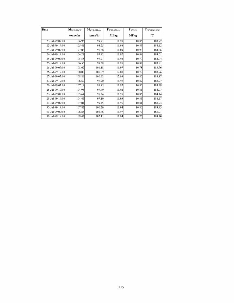
115
Date MWHBII,BFW MWHB,STEAM PWHB,STEAM PSTEAM TIN,WHBII,BFW
tonne/hr tonne/hr MPag MPag oC
23-Jul-99 07:00 106.95 99.71 11.98 10.85 183.9223-Jul-99 19:00 105.41 98.25 11.98 10.89 184.1224-Jul-99 07:00 97.03 90.68 11.89 10.93 184.2624-Jul-99 19:00 104.21 97.42 11.92 10.84 184.0125-Jul-99 07:00 105.55 98.71 11.92 10.79 184.0425-Jul-99 19:00 106.55 99.38 11.95 10.82 183.8126-Jul-99 07:00 108.62 101.18 11.97 10.78 183.7626-Jul-99 19:00 108.08 100.59 12.00 10.79 183.9627-Jul-99 07:00 108.86 100.93 12.03 10.80 183.8727-Jul-99 19:00 106.67 98.90 11.98 10.82 183.9728-Jul-99 07:00 107.18 99.45 11.97 10.80 183.9828-Jul-99 19:00 104.95 97.69 11.92 10.81 184.0729-Jul-99 07:00 105.64 98.24 11.95 10.85 184.1429-Jul-99 19:00 104.45 97.19 11.93 10.83 184.1730-Jul-99 07:00 107.01 99.45 11.95 10.81 183.9330-Jul-99 19:00 107.82 100.29 11.94 10.80 183.9331-Jul-99 07:00 108.88 101.46 11.97 10.77 183.9131-Jul-99 19:00 109.42 102.11 11.94 10.75 184.10

116
APPENDIX B
GAS CONSTANTS AND EQUATIONS
The RKS EOS is used to model the process. Specifics of this EOS and the Shomate Equation can
be found in the following tables and equations.
Table B-1 Gas Component Properties
Gas TC K
PC*10-6 Paa
MWT σ reduced volume
shift
p RKS
param
∆hof,298
NH3 405.6 11.28 17.0304 0.0380 0.8779 -45.89806 N2 126.2 3.39 28.0134 -0.0111 0.3631 0 H2 33.2 1.3 2.0158 -0.0111 0.1061 0 He 5.2 0.227 4.00260 -0.0028 -0.1318 0 Ar 150.8 4.87 39.948 -0.0028 0.3632 0 CH4 190.6 4.6 16.0426 -0.0014 0.4068 -74.87310 Table B-2 Gas Component Shomate Constants from 298 K to 1400K
Gas A B C D E F NH3 19.99563 49.77119 -15.37599 1.921168 0.189174 -53.30667 N2 26.09200 8.218801 -1.976141 0.159274 0.044434 -7.989230 H2 33.10780 -11.50800 11.60930 -2.844400 -0.159665 -9.991971 He 20.79331 0 0 0 0 0 Ar 20.79331 0 0 0 0 0 CH4 -0.703029 108.4773 -42.52157 5.862788 0.678565 -76.84376
2 2
a C,iC,i
C,i
R Ta
PΩ
= (B.1)
b C,ii
C,i
R Tb
PΩ
= (B.2)
i C,ii
C,i
R Tc
Pσ
= (B.3)
i C,i ia a α= (B.4)
i j i j i,ji j
a y y a a (1-k ) = ∑∑ (B.5a)
0 1 2 K K T K T= + + (B.5b)

117
i ii
b y b= ∑ (B.6)
i ii
c y c= ∑ (B.7)
a i R,ii 2
R,i
PA
TαΩ
= (B.8)
b R,ii
R,i
PB
TΩ
= (B.9)
i R,ii
R,i
PC
Tσ
= (B.10)
2
a PA (R T)
= (B.11)
b PB R T
= (B.12)
c PC R T
= (B.13)
i i R,i 1 p (1- T )α = + (B.14)
i C,ii
C,i
c P
R Tσ = (B.15)
2i i ip 0.480 1.574 -0.176 ω ω= + (B.16)
0 k ji, ≈ [25] (B.17)
( )0 i j i j i,j j i i ji j
K y y ac ac (1-k ) (1 p p p p )= + + +∑∑ (B.18)
i i j j i j1 i j i j i,j
i j C,i C,j
p p p p p pK y y ac ac (1-k )
T T
+ + = +
∑∑ (B.19)
i j2 i j i j i,j
i j C,i C,j
p pK y y ac ac (1-k )
T T= ∑∑ (B.20)

118
APPENDIX C
MATLAB®, SIMULINK® AND MAPLE® CODE
Matlab®, Simulink® and Maple® files used throughout this thesis, for model development and case
studies, are listed here for convenience. Actual coding details, which include process design
parameters, are covered by the Saskferco and University of Alberta secrecy agreement[17] and are
not included here
Table C-1 Process Simulation Files
# Filename Description 1 WHBI.m S-Function for WHB I 2 WHBII.m S-Function for WHB II 3 GG.m S-Function for Gas-Gas Exchanger 4 R1.m S-Function for Reactor 1 (includes R1B1, R1B2 & R1PH) 5 R2.m S-Function for Reactor 2 6 dataWHBI.m Data File for E1.m s-function 7 dataWHBII.m Data File for E2.m s-function 8 dataGG.m Data File for E3.m s-function 9 dataR1.m Data File for R1.m s-function 10 dataR2.m Data File for R2.m s-function 11 init.m Initialize all state variables @ t=0, for s-functions 12 flowarea.m Subroutine for calculating available flow area 13 conversion.m Subroutine for calculating ammonia conversion 14 kinetics.m Subroutine for calculating reaction kinetics 15 mwt.m Subroutine for calculating the molecular weight of the synthesis gas 16 rks_act.m Subroutine for RKS fugacity calculations 17 rks_dh.m Subroutine for RKS enthalpy changes of ammonia system 18 rks_dh2.m Subroutine for RKS enthalpy changes of ammonia system with
different inlet and outlet pressures 19 rks_rho.m Subroutine for RKS EOS density calculation 20 steam.m Subroutine for steam tables fit equations 21 ammonia.mdl Ammonia process simulation
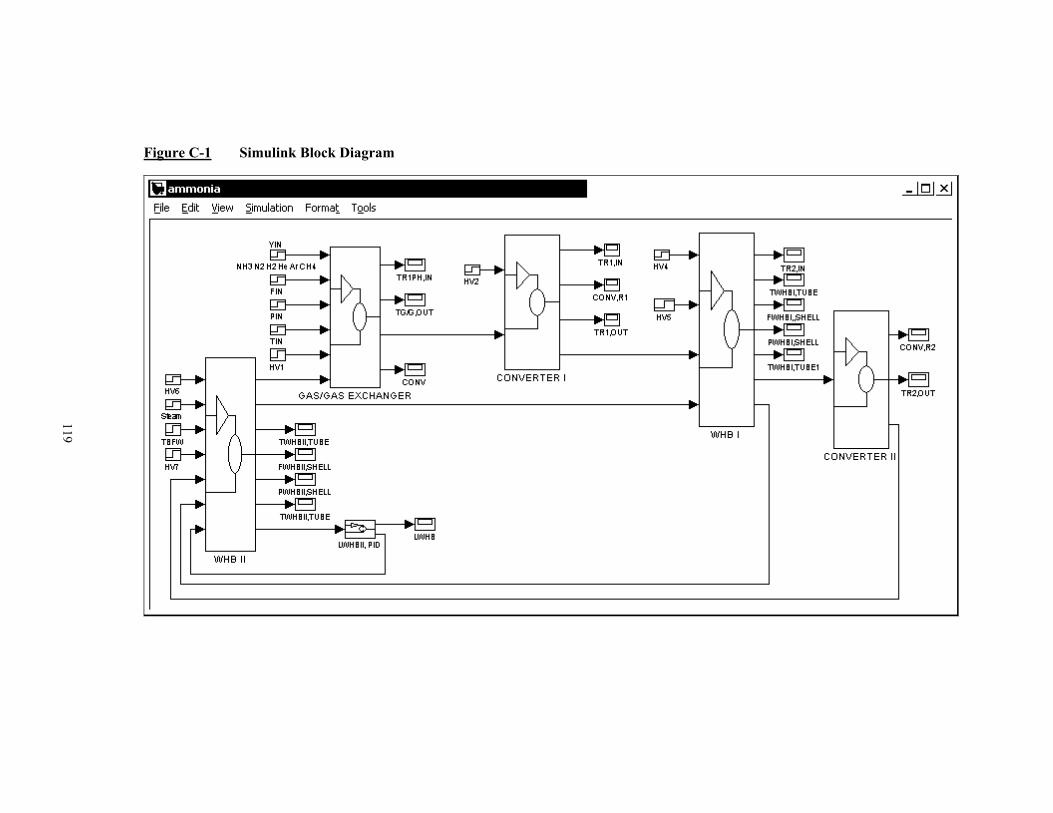
Figure C-1 Simulink Block Diagram
119

120
Table C-2 RKS EOS Calculations
# Filename Description 1 HR.mws Calculate residual enthalpy symbolically 2 HR.txt Calculate residual enthalpy symbolically Table C-3 Catalyst Effectiveness Parameter Update Files
# Filename Description 1 param_solve.m Invoke parameter update problem, plot solution 2 loadrx.m Subroutine to read plant data 3 rxdata.txt Plant data 4 param_update.m Initialize parameter update problem 5 set_options.m Subroutine to set options to solve Matlab functions 6 param_xo.m Subroutine to scale variables and set upper and lower limits 7 rks_abc.m Subroutine to calculate RKS thermodynamic properties for
initialization 8 rks_abc2.m Subroutine to calculate RKS thermodynamic properties for
initialization (excluding fugacity) 9 rks_act.m Subroutine for RKS fugacity calculations 10 rks_dh2.m Subroutine for RKS enthalpy changes of ammonia system with
different inlet and outlet pressures 11 rks_rho.m Subroutine for RKS EOS density calculation 12 mwt.m Subroutine for calculating the synthesis gas molecular weight 13 fnh3_out.m Subroutine to calculate reaction variables for initialization 14 fbal.m Subroutine to calculate variable estimates for initialization 15 param_con.m Equality and inequality constraints for parameter updates 16 param_opt.m Objective function for parameter updates 17 param_results.m Convert solved variables to appropriate units and scaling 18 Hmatrix.mws Calculate Φ as a function of process inputs 19 Hmatrix.txt Process calculations for parameter update matrix 20 Hvalues.txt Process values for parameter update matrix

121
Table C-4 Process Optimization Files
# Filename Description 1 nh3_solve.m Invoke optimization update problem, plot solution 2 loadnh3.m Subroutine to read plant data 3 nh3data.txt Plant data 4 nh3_update.m Initialize optimization update problem 5 set_options.m Subroutine to set options to solve Matlab functions 6 nh3_xo.m Subroutine to Scale variables and set upper and lower limits 7 rks_abc.m Subroutine to calculate RKS thermodynamic properties for
initialization 8 rks_abc2.m Subroutine to calculate RKS thermodynamic properties for
initialization (excluding fugacity) 9 rks_act.m Subroutine for RKS fugacity calculations 10 rks_dh.m Subroutine for RKS enthalpy changes of ammonia system 11 rks_rho.m Subroutine for RKS EOS density calculation 12 mwt.m Subroutine for calculating the synthesis gas molecular weight 13 flowarea.m Subroutine for calculating available flow area 14 fbal.m Subroutine to calculate variable estimates for initialization 15 steam.m Subroutine for steam tables fit equations 16 steam_tables.m Subroutine for steam table lookup values 17 ynh3_out2.m Subroutine for converter output variables 18 nh3_con.m Equality and inequality constraints for parameter updates 19 nh3_opt.m Objective function for parameter updates 20 nh3_results.m Subroutine to convert solved variables to appropriate units and
scaling Table C-5 State Space Matrices
# Filename Description 1 StateSpace.mws Calculate state space matrices 2 nh3_m1.txt State space equations 3 nh3_v1.txt Process values to determine local state space 4 obs_ctrl.m Check controllability and observability of full and reduced matrix 5 nh3_tf.m Evaluate state space properties – check stability, controller gain,
etc. Table C-6 Process Control Simulations
# Filename Description 1 ammonia_PID.mdl Ammonia process with PID control 2 ammonia_LQP.mdl Ammonia process with LQR control

122
APPENDIX D
PROCESS MODEL
Calculations and results of the process model not presented in Chapter 2 can be found in the
following sections.
D.1 Calculations
Equations D.1 to D.16 comprise the synthesis gas enthalpy, average heat capacity and average
density calculations as function of Equations 2.32, 2.33 and 2.41.
G/G,TUBE P,G/G,TUBE G/G,TUBE WHBII,TUBE G/G,TUBE R2h , C , = (T , T , P , )fρ ∆ R2y (D.1)
G/G,SHELL P,G/G,SHELL G/G,SHELL G/G,SHELL,IN G/G,SHELL IN,SGh , C , = (T , T , P , )fρ ∆ INy (D.2)
G/G,BY1 P,G/G,BY1 G/G,BY1 G/G,SHELL,IN G/G,BY IN,SGh , C , = (T , T , P , )fρ ∆ INy (D.3)
G/G,BY2 P,G/G,BY2 G/G,BY2 G/G,SHELL G/G,BY IN,SGh , C , = (T , T , P , )fρ ∆ INy (D.4)
R1PH,TUBE P,R1PH,TUBE R1PH,TUBE G/G,BY R1PH,TUBE IN,SGh ,C , = (T , T , P , )fρ ∆ INy (D.5)
R1PH,SHELL P,R1PH,SHELL R1PH,SHELL R1B1 R1PH,SHELL R1B1h ,C , = (T , T , P , )fρ ∆ R1B1y (D.6)
R1PH,BY1 P,R1PH,BY1 R1PH,BY1 G/G,BY R1PH,B IN,SGh ,C , = (T , T , P , )fρ ∆ INy (D.7)
G/G,BY2 P,G/G,BY2 R1PH,BY1 R1PH,TUBE R1PH,BY IN,SGh ,C , = (T , T , P , )fρ ∆ INy (D.8)
R1B1 P,R1B1 1 1 R1PH,B R1B1 IN,SG R1B1h ,C , = (T , T , P , P , )R B fρ ∆ INy (D.9)
R1B2 P,R1B2 R1B2 R1PH,SHELL R1B2 R1B1 R1B2h ,C , = (T , T , P , P , )fρ ∆ R1B1y (D.10)
WHBI,TUBE P,WHBI,TUBE WHBI,TUBE R1B2 WHBI,TUBE R1B2h ,C , = (T , T , P , )fρ ∆ R1B2y (D.11)
WHBI,BY1 P,WHBI,BY1 WHBI,BY1 R1B2 WHBI,BY R1B2h ,C , = (T , T , P , )fρ ∆ R1B2y (D.12)
WHBI,BY2 P,WHBI,BY2 WHBI,BY2 WHBI,TUBE WHBI,BY R1B2h , C , = (T , T , P , )fρ ∆ R1B2y (D.13)
R2 P,R2 R2 WHBI,B R2 R1B2 R2h , C , = (T , T , P , P , )fρ ∆ R1B2y (D.14)
WHBII,TUBE P,WHBII,TUBE WHBII,TUBE R2 WHBII,TUBE R2h C , = (T , T , P , )fρ ∆ R2y (D.15)
( )IN,SG,STP 0.101325 MPa, 293.15 K, fρ = INy (D.16)

123
Steam properties are expressed as a function of temperature in Equations D.17 to D.21
WHBI,BFW WHBI,STEAM P,WHBI,BFW WHBI,BFW WHBI,STEAM WHBI,STEAM WHBI,SHELL H , H , C , , , P = (T ) fρ ρ
(D.17)
WHBII,BFW,IN WHBII,BFW,IN WHBII,BFW-INH , = (T ) fρ (D.18)
WHBII,BFW-B P,WHBII,BFW-B WHBII,BFW-B WHBII,SHELL-BH , C , = (T )fρ (D.19)
WHBII,BFW-M P,WHBII,BFW-M WHBII,BFW-M WHBII,SHELL-MH , C , = (T )fρ (D.20)
WHBII,BFW-T WHBII,STEAM P,WHBII,BFW-T WHBII,BFW-T WHBII,STEAM WHBII,STEAMH , H , C , , , P ρ ρ
WHBII,SHELL-T= (T ) f (D.21)
Using Equation 2.54, the available flow area can be determined as follows in Equations
D.22 to D.33. Process valve and piping radii were provided by Saskferco[17].
( )G/G,SHELL G/G,SHELLAv = r , HV 100 % f = (D.22)
( )G/G,BY G/G,BY G/G,SHELLAv = r , HV f (D.23)
( )R1PH,TUBE R1PH,TUBEAv = r , HV 100 % f = (D.24)
( )R1PH,BY R1PH,BY R1PH,BYAv = R , HV f (D.25)
( )WHBI,TUBE WHBI,TUBEAv = R , HV 100 %f = (D.26)
( )WHBI,BY WHBI,BY WHBI,BYAv = R , HV f (D.27)
( )WHBI,BFW WHBI,BFWAv = r , HV 100 % f = (D.28)
( )WHBI,STEAM WHBI,STEAMAv = r , HV 100 % f = (D.29)
( )WHBII,BFW WHBII,BFW WHBII,BFWAv = r , HV f (D.30)
( )WHBII,BFW-T WHBII,BFW-T WHBII,BFW-TAv = r , HV f (D.31)
( )WHBII,BFW-B WHBII,BFW-BAv = r , HV 100 % f = (D.32)
( )WHBII,STEAM WHBII,STEAMAv = r , HV 100 % f = (D.33)
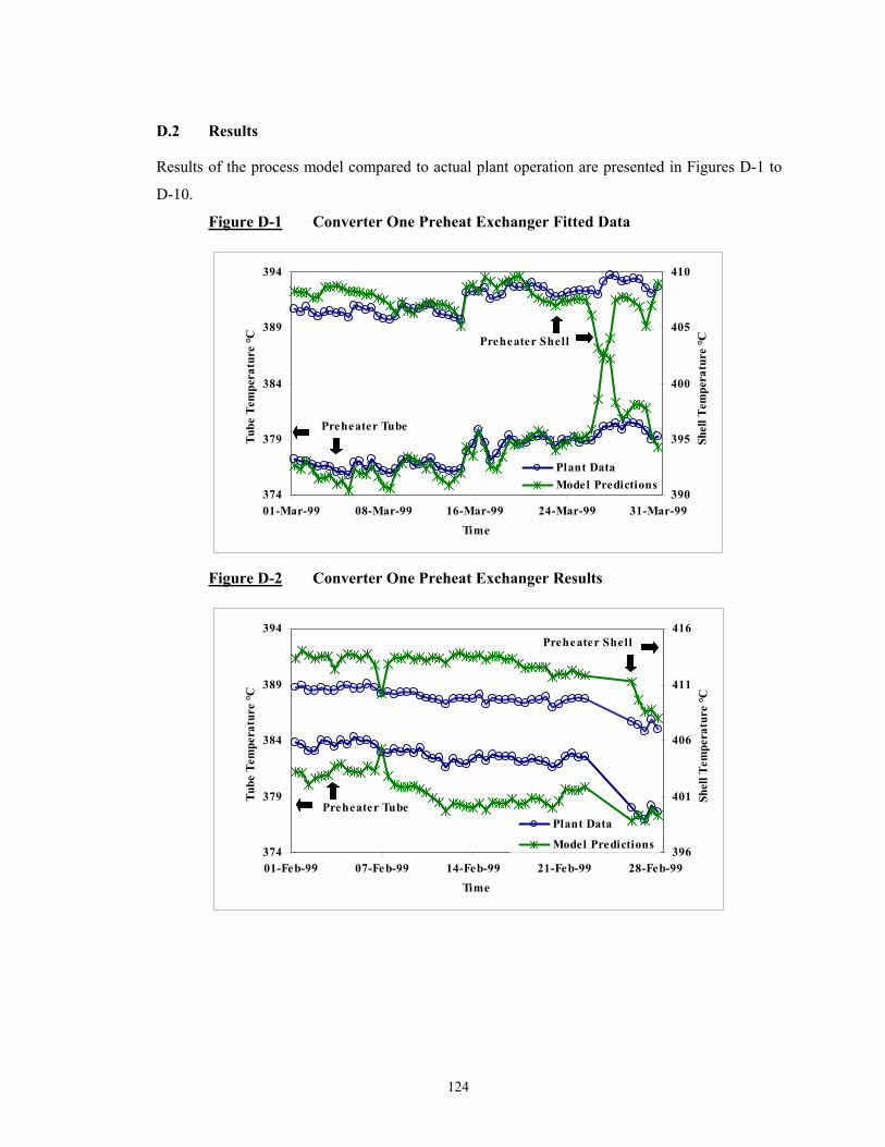
124
D.2 Results
Results of the process model compared to actual plant operation are presented in Figures D-1 to
D-10.
Figure D-1 Converter One Preheat Exchanger Fitted Data
374
379
384
389
394
01-Mar-99 08-Mar-99 16-Mar-99 24-Mar-99 31-Mar-99Time
Tube
Tem
pera
ture
°C
390
395
400
405
410
Shel
l Tem
pera
ture
°C
Plant DataModel Predictions
Preheater Tube
Preheater Shell
Figure D-2 Converter One Preheat Exchanger Results
374
379
384
389
394
01-Feb-99 07-Feb-99 14-Feb-99 21-Feb-99 28-Feb-99Time
Tube
Tem
pera
ture
°C
396
401
406
411
416
Shel
l Tem
pera
ture
°C
Plant Data
Model Predictions
Preheater Tube
Preheater Shell

125
Figure D-3 Converter One Bed Two Fitted Data
455
460
465
470
475
01-Mar-99 08-Mar-99 16-Mar-99 24-Mar-99 31-Mar-99Time
R1B
2 C
onve
rsio
n Te
mpe
ratu
re, °
C
Plant DataModel Predictions
Figure D-4 Converter One Bed Two Results
455
460
465
470
475
01-Feb-99 07-Feb-99 14-Feb-99 21-Feb-99 28-Feb-99Time
R1B
2 C
onve
rsio
n Te
mpe
ratu
re, °
C
Plant DataModel Predictions

126
Figure D-5 Converter Two Fitted Data
435
440
445
450
455
01-Mar-99 08-Mar-99 16-Mar-99 24-Mar-99 31-Mar-99Time
R2
Con
vers
ion
Tem
pera
ture
, °C
Plant DataModel Predictions
Figure D-6 Converter Two Results
435
440
445
450
455
01-Feb-99 07-Feb-99 14-Feb-99 21-Feb-99 28-Feb-99Time
R2
Con
vers
ion
Tem
pera
ture
, °C
Plant DataModel Predictions
c

127
Figure D-7 Waste Heat Boiler I Fitted Data
334
339
344
349
354
01-Mar-99 08-Mar-99 16-Mar-99 24-Mar-99 31-Mar-99Time
Tube
Tem
pera
ture
, °C
382
387
392
397
402
Bypa
ss T
empe
ratu
re, °
C
Plant DataModel Predictions
WHB I Tube
WHB I Tube Bypass
Figure D-8 Waste Heat Boiler I Results
340
345
350
355
360
01-Feb-99 07-Feb-99 14-Feb-99 21-Feb-99 28-Feb-99Time
Tube
Tem
pera
ture
, °C
384
389
394
399
404
Plant DataModel Predictions
WHB I Tube
WHB I Tube Bypass
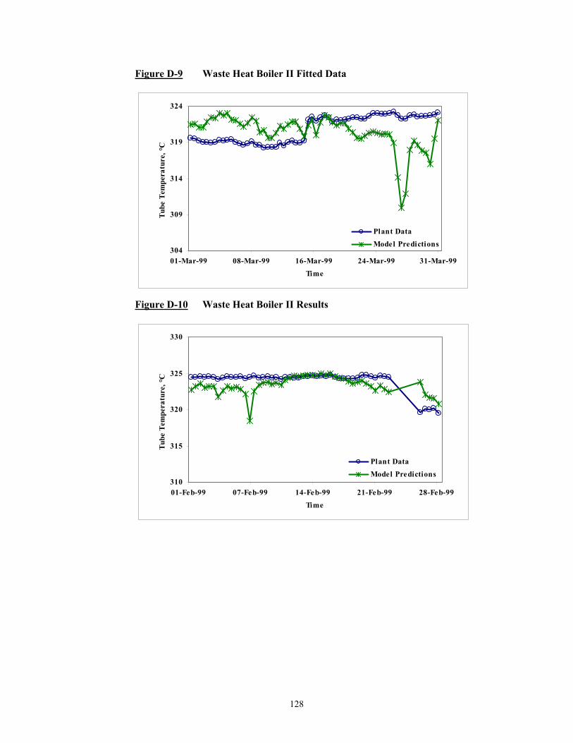
128
Figure D-9 Waste Heat Boiler II Fitted Data
304
309
314
319
324
01-Mar-99 08-Mar-99 16-Mar-99 24-Mar-99 31-Mar-99Time
Tube
Tem
pera
ture
, °C
Plant DataModel Predictions
Figure D-10 Waste Heat Boiler II Results
310
315
320
325
330
01-Feb-99 07-Feb-99 14-Feb-99 21-Feb-99 28-Feb-99Time
Tube
Tem
pera
ture
, °C
Plant DataModel Predictions

129
APPENDIX E
PARAMETER UPDATE RESULTS
The parameter update problems consist of 123 dependent variables, and 3 independent variables.
The objective function is posed to minimize the error between 4 measured plant variables and
process model predictions.
E.1 Dependent Variables
Three different cases of the parameter update problem are studied. Table E-1 lists the dependent
variables used in case one, the sum of squares.
Table E-1 Parameter Update Constraint Variables
Equation #
Variable Equation #
Variable Equation #
Variable
1 TR1B1 27 CR2,IN 58 – 63 aR1B2
2 TR1B2 28 CR1B1,OUT 64 – 69 aR2
3 TR2 29 CR1B2,OUT 70 – 75 yR1B1
4 rxnR1B1 30 CR2,OUT 76 – 81 yR1B2
5 rxnR1B2 31 CR1B1,OUT2 82 – 87 yR2
6 rxnR2 32 CR1B2,OUT2 88 – 93 y_A R1B12
7 AR1B1,IN 33 CR2,OUT2 94 – 99 y_A R1B22
8 AR1B2,IN 34 ZR1B1,IN 100 – 105 y_A R22
9 AR2,IN 35 ZR1B2,IN 106 hRR1B1,IN
10 AR1B1,OUT 36 ZR2,IN 107 hRR1B2,IN
11 AR1B2,OUT 37 ZR1B1,OUT 108 hRR2,IN
12 AR2,OUT 38 ZR1B2,OUT 109 hRR1B1,OUT
13 AR1B1,OUT2 39 ZR2,OUT 110 hRR1B2,OUT
14 AR1B2,OUT2 40 ZR1B1,OUT2 111 hRR2,OUT
15 AR2,OUT2 41 ZR1B2,OUT2 112 ∆hR1B1
16 BR1B1,IN 42 ZR2,OUT2 113 ∆hR1B2
17 BR1B2,IN 43 φNH3,R1B1 114 ∆hR2
18 BR2,IN 44 φNH3,R1B2 115 k_R1B1

130
Equation #
Variable Equation #
Variable Equation #
Variable
19 BR1B1,OUT 45 φNH3,R2 116 k_R1B2
20 BR1B2,OUT 46 φN2,R1B1 117 k_R2
21 BR2,OUT 47 φN2,R1B2 118 KpR1B1
22 BR1B1,OUT2 48 φN2,R2 119 KpR1B2
23 BR1B2,OUT2 49 φH2,R1B1 120 KpR2
24 BR2,OUT2 50 φH2,R1B2 121 HrxnR1B1
25 CR1B1,IN 51 φH2,R2 122 HrxnR1B2
26 CR1B2,IN 52 – 57 aR1B1 123 HrxnR2
E.2 Intermediate Variables
Variables in Table E-1 are calculated using a steady-state form of the process equations identified
in Chapter 2. The exception to this is the use of the intermediate variables defined in Equations
E.34 to E.36 2 2
R1B1,i R1B1,i R1B1,OUT2,iy_A y A = (E.34)
2 2R1B2,i R1B2,i R1B2,OUT2,iy_A y A = (E.35)
2 2R2,i R2,i R2,OUT2,iy_A y A= (E.36)
E.3 Results
Results of the parameter update problem for R1B2 and R2 can be referenced in Figures E-1 to E-
4.

131
Figure E-1 R1B2 Dynamic Parameter Update
1.2
1.3
1.4
1.5
1.6
01-Feb-99 07-Feb-99 14-Feb-99 21-Feb-99 28-Feb-99Time
Exte
nt o
f For
war
d R
eact
ion,
--
Case 1aCase 1bCase 2
Figure E-2 R2 Dynamic Parameter Update
1.1
1.2
1.3
1.4
1.5
01-Feb-99 07-Feb-99 14-Feb-99 21-Feb-99 28-Feb-99Time
Cat
alys
t Eff
ectiv
enes
s Fac
tor,
--
Case 1aCase 1bCase 2

132
Figure E-3 R1B2 Conversion Temperature Error
-12
-8
-4
0
4
8
12
01-Feb-99 07-Feb-99 14-Feb-99 21-Feb-99 28-Feb-99Time
R1B
2 C
onve
rsio
n Te
mpe
ratu
re E
rror
, °C
Case 1aCase 1bCase 2
Figure E-4 R2 Conversion Temperature Error
-12
-6
0
6
12
01-Feb-99 07-Feb-99 14-Feb-99 21-Feb-99 28-Feb-99Time
R2
Con
vers
ion
Tem
pera
ture
Err
or, °
C
Case 1aCase 1bCase 2
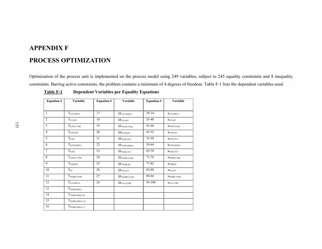
APPENDIX F
PROCESS OPTIMIZATION
Optimization of the process unit is implemented on the process model using 249 variables, subject to 245 equality constraints and 8 inequality
constraints. Barring active constraints, the problem contains a minimum of 4 degrees of freedom. Table F-1 lists the dependent variables used.
Table F-1 Dependent Variables per Equality Equations
Equation # Variable Equation # Variable Equation # Variable
1 TG/G,SHELL 17 ∆h G/G,SHELL 29-34 aG/G,SHELL
2 TG/G,BY 18 ∆h G/G,BY 35-40 aG/G,BY
3 TR1PH,TUBE 19 ∆h R1PH,TUBE 41-46 aR1PH,TUBE
4 TR1PH,BY 20 ∆h R1PH,BY 47-52 aR1PH,BY
5 TR1B1 21 ∆h R1B1,OUT 53-58 aR1B1,OUT
6 TR1PH,SHELL 22 ∆h R1PH,SHELL 59-64 aR1PH,SHELL
7 TR1B2 23 ∆h R1B2,OUT 65-70 aR1B2,OUT
8 TWHB1,TUBE 24 ∆h WHBI,TUBE 71-76 aWHBI,TUBE
9 TWHB,BY 25 ∆h WHBI,BY 77-82 aWHBI,B
10 TR2 26 ∆h R2,OUT 83-88 aR2,OUT
11 TWHBII,TUBE 27 ∆h WHBII,TUBE 89-94 aWHBII,TUBE
12 TG/G,SHELL 28 ∆h G/G,TUBE 95-100 aG/G,TUBE
13 TWHBI,SHELL
14 TWHBII,SHELL-B
15 TWHBII,SHELL-M
16 TWHBII,SHELL-T
133

Table F-1 Dependent Variables per Equality Equations (cont’d) Equation # Variable Equation # Variable Equation # Variable Equation # Variable Equation # Variable
101 ASG,IN 117 BSG,IN 133 CSG,IN 149 ZSG,IN 165 hRSG,IN
102 AG/G,SHELL 118 BG/G,SHELL 134 CG/G,SHELL 150 ZG/G,SHELL 166 hRG/G,SHELL
103 AG/G,BY 119 BG/G,BY 135 CG/G,BY 151 ZG/G,BY 167 hRG/G,B
104 AR1PH,TUBE 120 BR1PH,TUBE 136 CR1PH,TUBE 152 ZR1PH,TUBE 168 hRR1PH,TUBE
105 AR1PH,BY 121 BR1PH,BY 137 CR1PH,BY 153 ZR1PH,BY 169 hRR1PH,BY
106 AR1B1,OUT 122 BR1B1,OUT 138 CR1B1,OUT 154 ZR1B1,OUT 170 hRR1B1,OUT
107 AR1B1,OUT2 123 BR1B1,OUT2 139 CR1B1,OUT2 155 ZR1B1,OUT2 171 hRR1B1,OUT2
108 AR1PH,SHELL 124 BR1PH,SHELL 140 CR1PH,SHELL 156 ZR1PH,SHELL 172 hRR1PH,SHELL
109 AR1B2,OUT 125 BR1B2,OUT 141 CR1B2,OUT 157 ZR1B2,OUT 173 hRR1B2,OUT
110 AR1B2,OUT2 126 BR1B2,OUT2 142 CR1B2,OUT2 158 ZR1B2,OUT2 174 hRR1B2,OUT2
111 AWHBI,TUBE 127 BWHBI,TUBE 143 CWHBI,TUBE 159 ZWHBI,TUBE 175 hRWHBI,TUBE
112 AWHBI,BY 128 BWHBI,BY 144 CWHBI,BY 160 ZWHBI,BY 176 hRWHBI,BY
113 AR2,OUT 129 BR2,OUT 145 CR2,OUT 161 ZR2,OUT 177 hRR2,OUT
114 AR2,OUT2 130 BR2,OUT2 146 CR2,OUT2 162 ZR2,OUT2 178 hRR2,OUT2
115 AWHBII,TUBE 131 BWHBII,TUBE 146 CWHBII,TUBE 163 ZWHBII,TUBE 179 hRWHBII,TUBE
116 AG/G,TUBE 132 BG/G,TUBE 148 CG/G,TUBE 164 ZG/G,TUBE 180 hRG/G,TUBE
134
Table F-1 Dependent Variables per Equality Equations (cont’d) Equation # Variable Equation # Variable Equation # Variable Equation # Variable Equation # Variable
181 rxnR1B1 184 KpR1B1 187 k_R1B1 190-195 yR1B1 208 HrxnR1B1
182 rxnR1B2 185 KpR1B2 188 k_R1B2 196-201 yR1B2 209 HrxnR1B2
183 rxnR2 186 KpR2 189 k_R2 202-207 yR2 210 HrxnR2
211 φNH3,R1B1 214 φN2,R1B1 217 φH2,R1B1 220-225 y_A R1B12
212 φNH3,R1B2 215 φN2,R1B2 218 φH2,R1B2 226-231 y_A R1B22
213 φNH3,R2 216 φN2,R2 219 φH2,R2 232-237 y_A R22
238 QG/G 242 ffG/G,SHELL
239 QR1PH 243 ffR1PH,TUBE
240 QWHBI 244 ffWHBI,TUBE
241 QWHBII 245 ffWHBII,SHELL-B
135
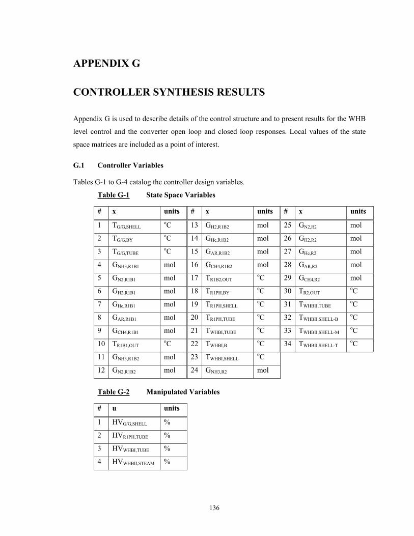
136
APPENDIX G
CONTROLLER SYNTHESIS RESULTS
Appendix G is used to describe details of the control structure and to present results for the WHB
level control and the converter open loop and closed loop responses. Local values of the state
space matrices are included as a point of interest.
G.1 Controller Variables
Tables G-1 to G-4 catalog the controller design variables.
Table G-1 State Space Variables
# x units # x units # x units
1 TG/G,SHELL oC 13 GH2,R1B2 mol 25 GN2,R2 mol
2 TG/G,BY oC 14 GHe,R1B2 mol 26 GH2,R2 mol
3 TG/G,TUBE oC 15 GAR,R1B2 mol 27 GHe,R2 mol
4 GNH3,R1B1 mol 16 GCH4,R1B2 mol 28 GAR,R2 mol
5 GN2,R1B1 mol 17 TR1B2,OUT oC 29 GCH4,R2 mol
6 GH2,R1B1 mol 18 TR1PH,BY oC 30 TR2,OUT oC
7 GHe,R1B1 mol 19 TR1PH,SHELL oC 31 TWHBII,TUBE oC
8 GAR,R1B1 mol 20 TR1PH,TUBE oC 32 TWHBII,SHELL-B oC
9 GCH4,R1B1 mol 21 TWHBI,TUBE oC 33 TWHBII,SHELL-M oC
10 TR1B1,OUT oC 22 TWHBI,B oC 34 TWHBII,SHELL-T oC
11 GNH3,R1B2 mol 23 TWHBI,SHELL oC
12 GN2,R1B2 mol 24 GNH3,R2 mol
Table G-2 Manipulated Variables
# u units
1 HVG/G,SHELL %
2 HVR1PH,TUBE %
3 HVWHBI,TUBE %
4 HVWHBII,STEAM %
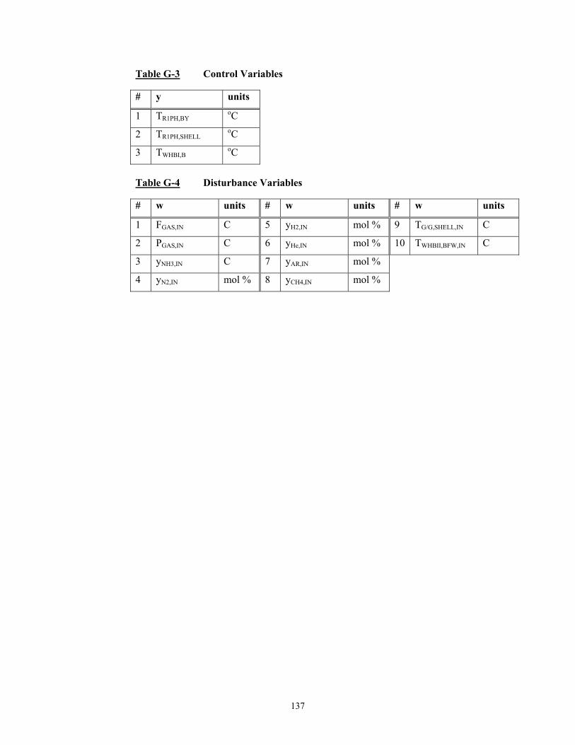
137
Table G-3 Control Variables
# y units
1 TR1PH,BY oC
2 TR1PH,SHELL oC
3 TWHBI,B oC
Table G-4 Disturbance Variables
# w units # w units # w units
1 FGAS,IN C 5 yH2,IN mol % 9 TG/G,SHELL,IN C
2 PGAS,IN C 6 yHe,IN mol % 10 TWHBII,BFW,IN C
3 yNH3,IN C 7 yAR,IN mol %
4 yN2,IN mol % 8 yCH4,IN mol %

G.2 Open Loop Responses
RGA analysis and PID tuning are accomplished by observing the open loop response of the control variables to perturbations in the manipulated
variables. Results can be found in Figures G-1 to G-5.
Figure G-1 CV1 Step, Open Loop
-15
-11
-7
-3
1
0 4 8 12 16 20 24 28 32
Time, minutes
Con
trol
Var
iabl
e 1,
∆o C
-5
20
45
70
95
Man
ipul
ated
Var
iabl
e 2,
∆
%
CV1 = TR1B1,IN
MV2 = HVR1PH,TUBE
-4
-2
0
2
4
0 4 8 12 16 20 24 28 32
Time, minutes
Stea
m P
rodu
ctio
n, ∆
tonn
e/hr
138
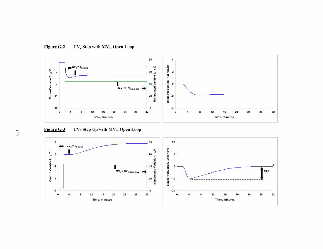
Figure G-2 CV2 Step with MV1, Open Loop
-15
-11
-7
-3
1
0 4 8 12 16 20 24 28 32
Time, minutes
Con
trol
Var
iabl
e 2,
∆o C
-5
20
45
70
95
Man
ipul
ated
Var
iabl
e 1,
∆
%CV2 = TR1B2,IN
MV1 = HVG/G,SHELL
-4
-2
0
2
4
0 4 8 12 16 20 24 28 32
Time, minutes
Stea
m P
rodu
ctio
n, ∆
tonn
e/hr
Figure G-3 CV2 Step Up with MV4, Open Loop
-6
-4
-2
0
2
0 4 8 12 16 20 24 28 32
Time, minutes
Con
trol
Var
iabl
e 2,
∆o C
-5
20
45
70
95
Man
ipul
ated
Var
iabl
e 4,
∆
%
CV2 = TR1B2,IN
MV4 = HVWHBII,STEAM
-20
-10
0
10
20
0 4 8 12 16 20 24 28 32
Time, minutes
Stea
m P
rodu
ctio
n, ∆
tonn
e/hr
10.2
139

Figure G-4 CV2 Step Down with MV4, Open Loop
-6
-4
-2
0
2
30 34 38 42 46 50 54 58 62
Time, minutes
Con
trol
Var
iabl
e 2,
∆o C
-5
20
45
70
95
Man
ipul
ated
Var
iabl
e 4,
∆
%CV2 = TR1B2,IN
MV4 = HVWHBII,STEAM
-20
-10
0
10
20
30 34 38 42 46 50 54 58 62
Time, minutes
Stea
m P
rodu
ctio
n, ∆
tonn
e/hr
12.5
Figure G-5 CV3 Step, Open Loop
-56
-40
-24
-8
8
0 4 8 12 16 20 24 28 32
Time, minutes
Con
trol
Var
iabl
e 3,
∆o C
-75
-25
25
75
Man
ipul
ated
Var
iabl
e 3,
∆
%
CV3 = TR2,IN
MV3 = HVWHBI,TUBE
-4
-2
0
2
4
0 4 8 12 16 20 24 28 32
Time, minutes
Stea
m P
rodu
ctio
n, ∆
tonn
e/hr
140

G.3 State Space Matrices
Local analysis of controller observability and controllability is evaluated from the following state space matrices. Tables G-5 to G-8 represent the
local state space with 34 state variables. Eliminating composition from the state space to remove near-zero eigenvalues resulted in 16 state space
variables. The corresponding state space matrices are presented in Table G-9 to G-11.
Table G-5 Local Value of A(x,u,w) Matrix
A = -1.96 0 1.55 0 0 0 0 0 0 0 0 0 0 0 0 0 0 0 0 0 0 0 0 0 0 0 0 0 0 0 1.55 0 0 0
98.34 -98.34 0 0 0 0 0 0 0 0 0 0 0 0 0 0 0 0 0 0 0 0 0 0 0 0 0 0 0 0 0 0 0 0
5.60 0 -6.94 0 0 0 0 0 0 0 0 0 0 0 0 0 0 0 0 0 0 0 0 0.00 -0.01 0.00 0.00 -0.02 0.00 0 -4.19 0 0 0
0 0 0 -60.38 19.97 6.11 -4.20 4.57 -1.10 2.16 0 0 0 0 0 0 0 0 0 0 0 0 0 0 0 0 0 0 0 0 0 0 0 0
0 0 0 26.59 -20.15 -2.07 4.06 17.30 8.42 -1.08 0 0 0 0 0 0 0 0 0 0 0 0 0 0 0 0 0 0 0 0 0 0 0 0
0 0 0 81.26 13.71 -29.93 12.54 55.42 26.65 -3.24 0 0 0 0 0 0 0 0 0 0 0 0 0 0 0 0 0 0 0 0 0 0 0 0
0 0 0 0.39 0.65 0.05 -23.81 0.92 0.37 0 0 0 0 0 0 0 0 0 0 0 0 0 0 0 0 0 0 0 0 0 0 0 0 0
0 0 0 1.13 1.86 0.13 0.27 -21.25 1.07 0 0 0 0 0 0 0 0 0 0 0 0 0 0 0 0 0 0 0 0 0 0 0 0 0
0 0 0 4.54 7.47 0.54 1.07 10.65 -19.62 0 0 0 0 0 0 0 0 0 0 0 0 0 0 0 0 0 0 0 0 0 0 0 0 0
0 0 0 -0.32 0.10 0.04 -0.04 -0.04 -0.04 -2.72 0 0 0 0 0 0 0 2.63 0 0 0 0 0 0 0 0 0 0 0 0 0 0 0 0
0 0 0 19.78 -6.77 -0.49 -0.97 -9.66 -3.88 0 -21.99 10.48 2.36 -0.69 7.21 2.02 -18.82 0 0 0 0 0 0 0 0 0 0 0 0 0 0 0 0 0
0 0 0 -6.29 13.55 -0.74 -1.48 -14.76 -5.93 0 8.53 -12.20 -0.51 1.69 9.82 4.38 9.41 0 0 0 0 0 0 0 0 0 0 0 0 0 0 0 0 0
0 0 0 -20.37 -33.51 21.49 -4.79 -47.78 -19.19 0 26.61 14.21 -17.77 5.31 31.86 14.10 28.23 0 0 0 0 0 0 0 0 0 0 0 0 0 0 0 0 0
0 0 0 -0.39 -0.65 -0.05 23.81 -0.92 -0.37 0 0.27 0.44 0.03 -16.31 0.63 0.25 0 0 0 0 0 0 0 0 0 0 0 0 0 0 0 0 0 0
0 0 0 -1.13 -1.86 -0.13 -0.27 21.25 -1.07 0 0.77 1.27 0.09 0.18 -14.56 0.73 0 0 0 0 0 0 0 0 0 0 0 0 0 0 0 0 0 0
0 0 0 -4.54 -7.47 -0.54 -1.07 -10.65 19.62 0 3.11 5.12 0.37 0.73 7.30 -13.45 0 0 0 0 0 0 0 0 0 0 0 0 0 0 0 0 0 0
0 0 0 0.00 0.01 0.00 0.00 0.01 0.00 0 -0.05 0.02 0.01 -0.01 -0.01 -0.01 -1.87 0 1.73 0 0 0 0 0 0 0 0 0 0 0 0 0 0 0
0 0 0 0 0 0 0 0 0 0 0 0 0 0 0 0 0 -6.33 0 6.33 0 0 0 0 0 0 0 0 0 0 0 0 0 0
0 3.34 0 0.00 -0.07 0.03 0.01 -0.12 0.01 5.50 0 0 0 0 0 0 0 0 -11.95 3.34 0 0 0 0 0 0 0 0 0 0 0 0 0 0
0 9.32 0 0 0 0 0 0 0 5.10 0 0 0 0 0 0 0 0 5.10 -19.77 0 0 0 0 0 0 0 0 0 0 0 0 0 0
0 0 0 0 0 0 0 0 0 0 0.00 -0.02 0.01 0.00 -0.03 0.00 0.84 0 0 0 -5.04 0 2.15 0 0 0 0 0 0 0 0 0 2.15 0
0 0 0 0 0 0 0 0 0 0 0.00 0.00 0.00 0.00 0.00 0.01 54.76 0 0 0 67.04 -121.79 0 0 0 0 0 0 0 0 0 0 0 0
0 0 0 0 0 0 0 0 0 0 0 0 0 0 0 0 0.02 0 0 0 0.02 0 -0.66 0 0 0 0 0 0 0 0 0 0.00 0
0 0 0 0 0 0 0 0 0 0 12.65 -6.13 -0.44 -0.88 -8.74 -3.51 0 0 0 0 0 0 0 -10.98 6.58 1.38 -0.17 5.34 1.71 -47.47 0 0 0 0
0 0 0 0 0 0 0 0 0 0 -3.86 10.03 -0.46 -0.91 -9.05 -3.64 0 0 0 0 0 0 0 4.04 -7.39 -0.29 0.87 5.22 2.31 23.73 0 0 0 0
0 0 0 0 0 0 0 0 0 0 -12.60 -20.73 14.88 -2.96 -29.56 -11.87 0 0 0 0 0 0 0 12.72 7.72 -10.44 2.76 17.08 7.51 71.20 0 0 0 0
0 0 0 0 0 0 0 0 0 0 -0.27 -0.44 -0.03 16.31 -0.63 -0.25 0 0 0 0 0 0 0 0.16 0.26 0.02 -9.59 0.37 0.15 0 0 0 0 0
0 0 0 0 0 0 0 0 0 0 -0.77 -1.27 -0.09 -0.18 14.56 -0.73 0 0 0 0 0 0 0 0.46 0.75 0.05 0.11 -8.56 0.43 0 0 0 0 0
0 0 0 0 0 0 0 0 0 0 -3.11 -5.12 -0.37 -0.73 -7.30 13.45 0 0 0 0 0 0 0 1.83 3.01 0.22 0.43 4.29 -7.91 0 0 0 0 0
0 0 0 0 0 0 0 0 0 0 0.00 0.00 0.00 0.00 0.00 0.00 0 0 0 0 0 1.02 0 -0.01 0.01 0.00 0.00 0.00 0.00 -1.18 0 0 0 0
0 0 0 0 0 0 0 0 0 0 0 0 0 0 0 0 0 0 0 0 0 0 0 0.00 -0.02 0.01 0.00 -0.03 0.00 2.27 -5.99 1.94 0 0
0 0 0 0 0 0 0 0 0 0 0 0 0 0 0 0 0 0 0 0 0 0 -0.40 0 0 0 0 0 0 0.03 0.03 -0.07 0.00 -1.41
0 0 0 0 0 0 0 0 0 0 0 0 0 0 0 0 0 0 0 0 0 0 0.00 0 0 0 0 0 0 0 0 0.12 -0.12 0.00
0 0 0 0 0 0 0 0 0 0 0 0 0 0 0 0 0 0 0 0 0 0 0.05 0 0 0 0 0 0 0 0 0.77 0.47 -1.33
141

142
Table G-6 Local Value of B(x,u,w) Matrix
B=
0.063 0 0 0 -15.287 0 0 0 0 0 0 0 0 0 0 0 0 0 0 0 0 0 0 0 0 0 0 0 0 0 0 0 0 0 0 0 0 0 0 0 0 0 0 0 0 0 0 0 0 0 0 0 0 0 0 0 0 0 0 0 0 0 0 0 0 0 0 0 0 -2.191 0 0 0 0 0 0 0 5.076 0 0 0 0 -1.733 0 0 0 0.027 0 0 0 0 0 0 0 0 0 0 0 0 0 0 0 0 0 0 0 0 0 0 0 0 0 0 0 0 0 0 0 0 0 0 0 0 0 0 0 0 0.011 0 0 0 -0.044 0 0 0 -0.001

Table G-7 C Matrix
C=
0 0 0 0 0 0 0 0 0 0 0 0 0 0 0 0 0 1 0 0 0 0 0 0 0 0 0 0 0 0 0 0 0 0 0 0 0 0 0 0 0 0 0 0 0 0 0 0 0 0 0 0 1 0 0 0 0 0 0 0 0 0 0 0 0 0 0 0 0 0 0 0 0 0 0 0 0 0 0 0 0 0 0 0 0 0 0 0 0 1 0 0 0 0 0 0 0 0 0 0 0 0
143
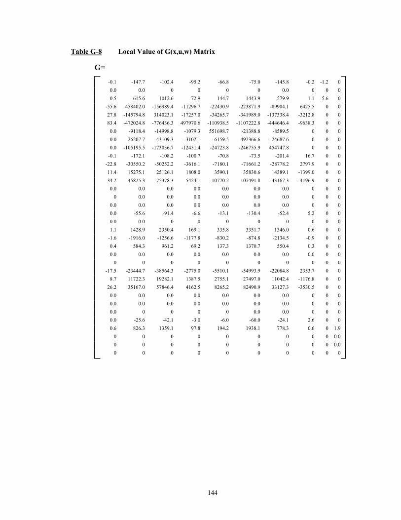
144
Table G-8 Local Value of G(x,u,w) Matrix
G=
-0.1 -147.7 -102.4 -95.2 -66.8 -75.0 -145.8 -0.2 -1.2 0 0.0 0.0 0 0 0 0 0.0 0 0 0 0.5 615.6 1012.6 72.9 144.7 1443.9 579.9 1.1 5.6 0 -55.6 458402.0 -156989.4 -11296.7 -22430.9 -223871.9 -89904.1 6425.5 0 0 27.8 -145794.8 314023.1 -17257.0 -34265.7 -341989.0 -137338.4 -3212.8 0 0 83.4 -472024.8 -776436.3 497970.6 -110938.5 -1107222.8 -444646.4 -9638.3 0 0 0.0 -9118.4 -14998.8 -1079.3 551698.7 -21388.8 -8589.5 0 0 0 0.0 -26207.7 -43109.3 -3102.1 -6159.5 492366.6 -24687.6 0 0 0 0.0 -105195.5 -173036.7 -12451.4 -24723.8 -246755.9 454747.8 0 0 0 -0.1 -172.1 -108.2 -100.7 -70.8 -73.5 -201.4 16.7 0 0 -22.8 -30550.2 -50252.2 -3616.1 -7180.1 -71661.2 -28778.2 2797.9 0 0 11.4 15275.1 25126.1 1808.0 3590.1 35830.6 14389.1 -1399.0 0 0 34.2 45825.3 75378.3 5424.1 10770.2 107491.8 43167.3 -4196.9 0 0 0.0 0.0 0.0 0.0 0.0 0.0 0.0 0 0 0 0 0.0 0.0 0.0 0.0 0.0 0.0 0 0 0 0.0 0.0 0.0 0.0 0.0 0.0 0.0 0 0 0 0.0 -55.6 -91.4 -6.6 -13.1 -130.4 -52.4 5.2 0 0 0.0 0.0 0 0 0 0 0 0 0 0 1.1 1428.9 2350.4 169.1 335.8 3351.7 1346.0 0.6 0 0 -1.6 -1916.0 -1256.6 -1177.8 -830.2 -874.8 -2134.5 -0.9 0 0 0.4 584.3 961.2 69.2 137.3 1370.7 550.4 0.3 0 0 0.0 0.0 0.0 0.0 0.0 0.0 0.0 0.0 0 0 0 0 0 0 0 0 0 0 0 0 -17.5 -23444.7 -38564.3 -2775.0 -5510.1 -54993.9 -22084.8 2353.7 0 0 8.7 11722.3 19282.1 1387.5 2755.1 27497.0 11042.4 -1176.8 0 0 26.2 35167.0 57846.4 4162.5 8265.2 82490.9 33127.3 -3530.5 0 0 0.0 0.0 0.0 0.0 0.0 0.0 0.0 0 0 0 0.0 0.0 0.0 0.0 0.0 0.0 0.0 0 0 0 0.0 0 0 0 0 0.0 0.0 0 0 0 0.0 -25.6 -42.1 -3.0 -6.0 -60.0 -24.1 2.6 0 0 0.6 826.3 1359.1 97.8 194.2 1938.1 778.3 0.6 0 1.9 0 0 0 0 0 0 0 0 0 0.0 0 0 0 0 0 0 0 0 0 0.0 0 0 0 0 0 0 0 0 0 0

Table G-9 Local Value of A(x,u,w) Matrix – Reduced and Scaled
A=
-0.0326 0 0.0258 0 0 0 0 0 0 0 0 0 0.0258 0 0 0 1.6389 -1.6389 0 0 0 0 0 0 0 0 0 0 0 0 0 0 0.0934 0 -0.1156 0.0000 0.0000 0 0 0 0 0 0 0.0001 -0.0699 0 0 0 0 0 0 -0.0456 0.0000 0.0438 0 0 0 0 0 0.0000 0 0 0 0 0 0 0 0.0000 -0.0304 0 0.0289 0 0 0 0 0.0000 0 0 0 0 0 0 0 0 0 -0.1056 0 0.1056 0 0 0 0 0 0 0 0 0 0.0557 0 0.0916 0.0000 0 -0.1991 0.0557 0 0 0 0.0000 0 0 0 0 0 0.1553 0 0.0849 0 0 0.0849 -0.3295 0 0 0 0 0 0 0 0 0 0 0 0.0000 0.0141 0 0 0 -0.0840 0 0.0358 0.0000 0 0 0.0358 0 0 0 0 0.0000 0.9126 0 0 0 1.1174 -2.0299 0 0.0000 0 0 0 0 0 0 0 0 0.0004 0 0 0 0.0004 0 -0.0110 0 0 0 -0.0001 0 0 0 0 0.0000 0.0002 0 0 0 0 0.0169 0 -0.0187 0 0 0 0 0 0 0 0.0000 0.0000 0 0 0 0 0 0 0.0380 -0.0999 0.0323 0 0 0 0 0 0 0 0 0 0 0 0 -0.0067 0.0005 0.0005 -0.0012 0.0000 -0.0234 0 0 0 0 0 0 0 0 0 0 0.0000 0 0 0.0020 -0.0020 0.0000 0 0 0 0 0 0 0 0 0 0 0.0008 0 0 0.0128 0.0078 -0.0221
145

146
Table G-10 Local Value of B(x,u,w) Matrix – Reduced and Scaled
B=
1.058E-03 0 0 0 -2.548E-01 0 0 0 0 0 0 0 0 0 0 0 0 0 0 0 0 -3.652E-02 0 0 0 0 0 0 0 8.461E-02 0 0 0 0 -2.889E-02 0 0 0 4.582E-04 0 0 0 0 0 0 0 0 0 0 0 0 0 0 0 0 1.822E-04 0 0 0 -7.398E-04 0 0 0 -2.177E-05
Table G-11 C Matrix – Reduced and Scaled
C=
0 0 0 0 0 1 0 0 0 0 0 0 0 0 0 0 0 0 0 0 0 0 1 0 0 0 0 0 0 0 0 0 0 0 0 0 0 0 0 0 0 1 0 0 0 0 0 0