university of calgary design and implementation of a 5
TRANSCRIPT

UNIVERSITY OF CALGARY
Design and Implementation of a 5-Channel CDMA Receiver for Mobile Position
Location
by
Alfredo Lopez
A THESIS
SUBMITTED TO THE FACULTY OF GRADUATE STUDIES
IN PARTIAL FULFILMENT OF THE REQUIREMENTS FOR THE
DEGREE OF MASTER OF SCIENCE
DEPARTMENT OF ELECTRICAL AND COMPUTER ENGINEERING
CALGARY, ALBERTA
September, 2006
© Alfredo López 2006

ii
UNIVERSITY OF CALGARY
FACULTY OF GRADUATE STUDIES
The undersigned certify that they have read, and recommend to the Faculty of
Graduate Studies for acceptance, a thesis entitled "DESIGN AND IMPLEMENTATION
OF A 5-CHANNEL CDMA RECEIVER FOR POSITION LOCATION" submitted by
ALFREDO LOPEZ in partial fulfilment of the requirements of the degree of MASTER
IN SCIENCE.
Supervisor, DR. JOHN NIELSEN, Department of Electrical and Computer Engineering
DR. GEOFFREY MESSIER, Department of Electrical and Computer Engineering
DR. SWAVIK SPIEWAK, Department of Mechanical and Manufacturing Engineering
DR. SEBASTIAN MAGIEROWSKI, Department of Electrical and Computer Engineering
Date

iii
Abstract
The purpose of this thesis is to provide a basic understanding behind the design wireless
location hardware in order to achieve an accurate position location. This thesis reports on
the design and implementation of a five-channel CDMA (PCS Band) receiver to be used
for Time of Arrival, Time Difference of Arrival, Angle of Arrival and a combination of
these. This thesis includes a review of these location techniques but they have not been
implemented.
The design receiver was developed to capture the larger possible amount of base station;
which is critical when the location of a mobile has to be estimated. The ability of
capturing weak pilot channel signal resides on a receiver having low noise figure.
Receiver’s parameters and performance are presented and measured in this thesis as well.

iv
Acknowledgements
I thank my parents for their unconditional support throughout my studies and for setting
an example to me of living. I thank my brother and sister for their support, and my wife,
Cynthia for her encouragement and support.
Special thanks to my supervisor, Dr John Nielsen, who gave me the opportunity of being
his student and arranged for me to be in this interesting project. For this, for his
marvelous patience and for providing me with technical suggestions at crucial moments
throughout the course of the project, he has earned my admiration.
The funding for this thesis was provided by the Department of Defence of Canada;
through the administration of Dr. Gerard Lachapelle (Department of Geomatics), who
also earned my admiration for his leadership and guidance; he provided invaluable
suggestions to the project as well.
I wouldn’t have gone as far as I have without the knowledge and help from Surendram K.
Shanmugam, a very skilled and qualified person in the field of signal processing, who
taught me and helped me to process the collected data in the last part of my work.
Fortunately, this project will not end with this thesis it will be continued by my two new
colleagues and friends Nazilla Salimi and Ahmad Reza Moghaddam who will perform
future tests, range measurements and position estimations.
I would also like to acknowledge the great help from Dingchen Lu, who programmed the
FPGA board and had to deal with the time synchronization.
Thanks to my friend, Rodolfo Peon, who always allowed me to use his laboratory and
precision tools.

v
Thanks to Dr Changlin Ma who also provided technical suggestions at various points of
this project.
Thanks to the University of Calgary technicians who helped me with the design of the
receiver’s layout.

vi
Dedication
To Melina and Milagros, my two beautiful nieces.
vii
Table of Contents
Approval Page..................................................................................................................... ii Abstract .............................................................................................................................. iii Acknowledgements............................................................................................................ iv Dedication .......................................................................................................................... vi Table of Contents.............................................................................................................. vii List of Tables .......................................................................................................................x List of Figures .................................................................................................................... xi List of Symbols, Abbreviations and Nomenclature...........................................................xv
CHAPTER ONE: THESIS INTRODUCTION ...................................................................1 1.1 Thesis Overview ........................................................................................................1 1.2 Overall objectives ......................................................................................................2 1.3 Summary of Contributions.........................................................................................3 1.4 Thesis Outline ............................................................................................................4
CHAPTER TWO: POSITION LOCATION TECHNIQUES .............................................6 2.1 Location Techniques..................................................................................................6
2.1.1 Received Signal Strength....................................................................................7 2.1.2 Angle of Arrival ..................................................................................................8 2.1.3 Time of Arrival .................................................................................................11 2.1.4 Time Difference of Arrival ...............................................................................14 2.1.5 Hybrid Location Techniques.............................................................................16
2.2 Non-Line of Sight Conditions..................................................................................16 2.3 Sources of Location Error........................................................................................18
2.3.1 Multipath Fading...............................................................................................18 2.3.2 NLOS Propagation............................................................................................19
2.4 Measure of Position Location Accuracy..................................................................20 2.4.1 Cramer-Rao Lower Bound................................................................................20 2.4.2 Circular Error Probability .................................................................................23 2.4.3 Geometric Dilution of Precision .......................................................................24
2.5 Detectability.............................................................................................................25 2.6 Power Control ..........................................................................................................25
CHAPTER THREE: THE FORWARD CDMA CHANNEL ...........................................27 3.1 The CDMA Technology Basics...............................................................................27 3.2 Direct Sequence Spread Spectrum...........................................................................28 3.3 The Forward CDMA Channel .................................................................................30
3.3.1 The Pilot Channel .............................................................................................30 3.3.2 The Synchronisation Channel ...........................................................................31 3.3.3 The Paging Channel ..........................................................................................31 3.3.4 The Traffic Channel ..........................................................................................31
3.4 The Pilot Channel ....................................................................................................31 3.5 Walsh Function ........................................................................................................33 3.6 Quadrature Spreading ..............................................................................................33 3.7 Baseband Filtering ...................................................................................................35

viii
3.8 Quadrature Phase Shift Keying (QPSK)..................................................................36 3.9 Frequency and Channel Specification .....................................................................38
CHAPTER FOUR: RECEIVER STRUCTURE................................................................41 4.1 Receiver Structure....................................................................................................41 4.2 Alternative Receiver Architectures..........................................................................43
4.2.1 Superheterodyne Receiver ................................................................................43 4.2.2 Homodyne Receiver..........................................................................................44 4.2.3 Low-IF Receivers..............................................................................................46
4.3 Receiver Front-End..................................................................................................46 4.3.1 Input RF Filter...................................................................................................49 4.3.2 LNA ..................................................................................................................50 4.3.3 Post LNA Filter.................................................................................................52 4.3.4 Linear Variable Gain Amplifier........................................................................52 4.3.5 Automatic Gain Control Loop ..........................................................................53 4.3.6 Mixer.................................................................................................................55 4.3.7 IF Filter .............................................................................................................56 4.3.8 IF Variable Gain Amplifier...............................................................................57 4.3.9 Demodulator .....................................................................................................58 4.3.10 Baseband Filter ...............................................................................................59
4.4 Digital Board............................................................................................................61
CHAPTER FIVE: RECEIVER PARAMETERS ..............................................................65 5.1 Receiver Performance..............................................................................................65 5.2 Noise Figure.............................................................................................................66
5.2.1 Minimum Detectable Signal .............................................................................68 5.3 Gain..........................................................................................................................69 5.4 Intermodulation Distortion ......................................................................................70 5.5 Third-Order Intercept Point .....................................................................................72 5.6 Receiver Dynamic Range ........................................................................................73 5.7 Receiver Selectivity .................................................................................................76 5.8 Receiver Sensitivity .................................................................................................76 5.9 Effect of Automatic Gain Control ...........................................................................77
CHAPTER SIX: TIME SYNCHRONIZATION AND LOCAL OSCILLATORS...........78 6.1 Base Stations Time Synchronization .......................................................................78 6.2 Receiver Synchronization ........................................................................................78 6.3 Local Oscillators ......................................................................................................80
6.3.1 Frequency offset................................................................................................81 6.4 Phase Noise and Spurious Outputs ..........................................................................82
6.4.1 Phase Noise .......................................................................................................82 6.4.2 Phase Noise Representation..............................................................................83 6.4.3 Phase Noise Measurement ................................................................................83
6.5 Allan Variance .........................................................................................................85
CHAPTER SEVEN: RECEIVER TEST ...........................................................................87 7.1 Receiver Test ...........................................................................................................87

ix
7.2 Single-Tone Desensitization ....................................................................................87 7.3 SNR vs. Integration Time ........................................................................................90 7.4 Phase Difference Stability .......................................................................................91
CHAPTER EIGHT: RANGE AND ANGLE MEASUREMENT ANALISYS................92 8.1 Introduction..............................................................................................................92 8.2 Post-mission processing...........................................................................................92
8.2.1 Two-Dimensional Acquisition..........................................................................93 8.3 CDMA Acquisition..................................................................................................93
8.3.1 Base Station Identification................................................................................94 8.3.2 CDMA Base Station Identification...................................................................98
8.4 Effect of Antenna Pattern ......................................................................................102 8.5 Effect of Predetection Integration Time ................................................................106 8.6 Receiver Repeatability Test ...................................................................................111 8.7 Field Tests..............................................................................................................116
8.7.1 Test Methodology ...........................................................................................116 8.7.2 Outdoor Field Test Specifications ..................................................................119 8.7.3 Field Test Performance Analysis ....................................................................120 8.7.4 Range Domain Analysis .................................................................................122
8.8 Antenna Array........................................................................................................125 8.9 Angle of Arrival Measurements ............................................................................132
CHAPTER NINE: CONCLUSIONS AND FUTURE WORK .......................................136 9.1 Conclusions............................................................................................................136 9.2 Future Work...........................................................................................................136
References........................................................................................................................138

x
List of Tables
Table 3-1 PCS Band Channel Assignment ....................................................................... 38
Table 4-1 RF Filter Parameters......................................................................................... 49
Table 4-2 LNA Specifications .......................................................................................... 51
Table 4-3 RF Variable Gain Amplifier Specifications ..................................................... 52
Table 4-4 Mixer Specifications......................................................................................... 55
Table 4-5 IF Filter Specifications ..................................................................................... 57
Table 4-6 Demodulator Specifications ............................................................................. 59
Table 6-1 TCXO Specifications........................................................................................ 80
Table 8-1 Estimated Range Measurements..................................................................... 110
Table 8-2 Estimated Frequency Offset For Different Trials........................................... 111
Table 8-3 Repeatability Analysis for Outdoor Antenna ................................................. 114
Table 8-4 Repeatability Analysis for Indoor Antenna.................................................... 114
Table 8-5 Residual Frequency Offset for Outdoor Field Test ........................................ 121
Table 8-6 Estimated Ranges ........................................................................................... 124
Table 8-7 GPS and CDMA Receiver Computed Range Differences ............................. 125
xi
List of Figures
Figure 2.1 Location Techniques ......................................................................................... 6
Figure 2.2Angle of Arrival Method.................................................................................... 9
Figure 2.3 Angle of Arrival Measurement........................................................................ 10
Figure 2.4 Time of Arrival Method .................................................................................. 12
Figure 2.5 Time Difference of Arrival Method ................................................................ 14
Figure 2.6 TOA with range measurement error................................................................ 17
Figure 2.7 Variance for Range Estimation Error .............................................................. 21
Figure 2.8 Geometry of the array...................................................................................... 22
Figure 2.9 Variance AOA Estimation Error ..................................................................... 23
Figure 2.10 Circle of Error Probability............................................................................ 24
Figure 3.1 Spread Spectrum Encoding ............................................................................. 29
Figure 3.2 Pilot Channel Structure.................................................................................... 32
Figure 3.3 Block Diagram of a linear feedback shift register........................................... 34
Figure 3.4 Baseband Filters Frequency Response ............................................................ 36
Figure 3.5 Forward CDMA channel signal constellation and phase transition ................ 37
Figure 3.6 CDMA Channel Assignment........................................................................... 39
Figure 3.7 Measured Frequency Spectrum ....................................................................... 40
Figure 4.1 Overall Architecture of the CDMA PCS Receiver.......................................... 42
Figure 4.2 Conventional Superheterodyne Receiver Architecture ................................... 43
Figure 4.3 Conventional Homodyne Receiver’s Architecture.......................................... 45
Figure 4.4 Picture of the developed receiver .................................................................... 47
Figure 4.5 Superheterodyne Receiver Block Diagram (Single Channel) ......................... 48

xii
Figure 4.6 RF Filter Frequency Response ........................................................................ 50
Figure 4.7 Power Detector and Inverter Output................................................................ 53
Figure 4.8 Block Diagram of the AGC Loop ................................................................... 54
Figure 4.9 IF Filter Frequency Response.......................................................................... 56
Figure 4.10 IF VGA Gain vs. Control Voltage................................................................. 58
Figure 4.11 Chebyshev Filter Characteristics (a) Frequency Response (b) Phase and
Group Delay.............................................................................................................. 60
Figure 4.12 Digital Board Block Diagram........................................................................ 62
Figure 4.13 Timing Diagram for the AD9059 .................................................................. 63
Figure 4.14 Picture of the digital board ............................................................................ 64
Figure 5.1 Noise Figure .................................................................................................... 68
Figure 5.2 Overall System Gain........................................................................................ 69
Figure 5.3 Output Spectrum of a Third-Tone Intermodulation Product........................... 70
Figure 5.4 Input Intercept Point ........................................................................................ 72
Figure 5.5 Intercept Diagram............................................................................................ 74
Figure 6.1 Timing Synchronization .................................................................................. 78
Figure 6.2 SNR vs. Frequency Offset (averaged)............................................................ 81
Figure 6.3 Output Spectrum of the RF LO ....................................................................... 84
Figure 6.4 Output Spectrum of the IF LO......................................................................... 85
Figure 7.1 Test settings ..................................................................................................... 88
Figure 7.2 Correlation Peaks with no interference signal................................................. 89
Figure 7.3 Correlation Peaks with interference signal...................................................... 89
Figure 7.4 SNR Vs Integration time ................................................................................. 90

xiii
Figure 7.5 Phase Difference.............................................................................................. 91
Figure 8.1 Frequency Spectrum Showing Probable CDMA Channels............................. 94
Figure 8.2 Received Signal Spectrum............................................................................... 97
Figure 8.3 Self-correlation Acquisition to Detect the Presence of CDMA Signal ........... 98
Figure 8.4 CDMA Correlation as a Function of Code Offset......................................... 100
Figure 8.5 CDMA Pilot Offsets Relative to GPS PPS Time Mark ................................ 101
Figure 8.6 (a) Directional Antenna (b) Omni-Directional Antenna ............................... 102
Figure 8.7 Correlation Plots for Different BSs. (a) Strongest BS (b) Second Strongest (c)
With Multipath Components (d) Directional antenna with higher gain ................. 105
Figure 8.8 Correlation Peak of the Strongest Base Station for Different Coherent
Integration Time...................................................................................................... 106
Figure 8.9 Correlation Peak of Strongest BS at Different Time Epochs (a) 0.08 s
Integration Time (b) 0.16 s Integration Time ......................................................... 108
Figure 8.10 Acquisition with 0.08 s Coherent Integration (a) Outdoor Antenna (b) Indoor
Antenna ................................................................................................................... 113
Figure 8.11 Correlation Peaks for Different Trials (a) BS # 1 Outdoor Antenna (b) BS #
1 Indoor Antenna .................................................................................................... 115
Figure 8.12 Outdoor Field Test Setup............................................................................. 117
Figure 8.13 Path Delay between Two Measurement Locations ..................................... 118
Figure 8.14 Map Showing Measurement Locations ....................................................... 120
Figure 8.15 Correlation Peak of the BS of Interest at all Measurement Locations (a)
Directional Antenna (b) Omni-Directional Antenna .............................................. 123
Figure 8.16 Antenna Array ............................................................................................. 126

xiv
Figure 8.17 Linear antenna array .................................................................................... 128
Figure 8.18 Uncompensated measured data ................................................................... 129
Figure 8.19 Compensated measured data ....................................................................... 129
Figure 8.20 Correlation peak .......................................................................................... 131
Figure 8.21 Measured data (Averaged) .......................................................................... 131
Figure 8.22 Linear Array Geometry ............................................................................... 132
Figure 8.23 LS Results.................................................................................................... 134
Figure 8.24 Estimated Error............................................................................................ 135

xv
List of Symbols, Abbreviations and Nomenclature
Symbol Definition ADC Analog to Digital Converter
BPF Band Pass Filter
BS Base Station
CDMA Channel Division Multiple-Access
CEP Circular Error Probability
CRLB Cramer-Rao Lower Bound
dBc/Hz Decibel below the carrier power per Hertz
DC Direct Current
E-911 Enhanced-911
GDOP Geometric Dilution Of Precision
GPS Global Positioning System
IF Intermediate Frequency
IF_LO IF Local Oscillator
IFVGA IF Variable Gain Amplifier
LNA Low Noise Amplifier
LO Local Oscillator
LOS Line Of Sight
LPF Low Pass Filter
Mcps Mega chips per second
MDS Minimum Detectable Signal
MS Mobile Station
NF Noise Figure
NLOS Non Line Of Sight
PCS Personal Communication System
PN Pseudo-noise
QPSK Quadrature Phase Shift Keying
RF Radio Frequency
RF_LO Radio Frequency Local Oscillator

xvi
RSS Received Signal Strength
Rx RF Receiver
SAW Surface Acoustic Wave
SFDR Spurious Free Dynamic Range
TCXO Temperature Controlled Crystal Oscillator
TDOA Time Difference Of Arrival
TOA Time Of Arrival
Tx RF Transmitter
VGA Variable Gain Amplifier

Chapter One
1
1
CHAPTER ONE: THESIS INTRODUCTION
1.1 Thesis Overview
Wireless location has been an active field of research over the past few decades. The
most recent applications of wireless location technologies have been in cellular radio
networks for subscriber location information for Enhanced-911 (E-911) safety services.
Recently, the number of E-911 calls placed by cellular telephones has grown
considerably in the United States; it is estimated that 170,000 calls a day are originated
from mobile phones [Saye05].
This significant increase in E-911 calls led to a 1996 Federal Communications
Commission (FCC) ruling requiring that all cellular and PCS operators to provide
location information for supporting E-911 safety services. The FCC Enhanced-911
regulations require cellular service providers to provide the position of cellular
subscribers calling 911; for reliable service, the FCC requires an accuracy of 50m of its
actual location for at least 67% of the calls and 150m for 95% of the calls for handset
based solutions. For network based solutions the requirements are, 100m for 67% of the
calls and 300m for 95% of the calls.
Wireless Location can be applied to several fields such as:
• Fleet Management: Emergency vehicle, police forces, fleet operators, taxi
companies and other services can make use of the wireless location system to
track and manage their fleet efficiently to minimize response times.
• Mobile Advertising: advertising and marketing can be targeted to a pre-defined
type of costumer. For example, stores will be able to track their costumer’s
Chapter One
2
2
location and attract them by flashing customized coupons on costumer’s wireless
devices [Saye05].
• Military Systems: wireless location systems can be used to find people in distress,
or to detect people that are causing distress in war zones.
• Fraud Detection: cellular phone fraud costs millions to the wireless industry; all
this cost represents higher phone usage rates to the wireless costumers. Wireless
location systems can be used to find and prosecute the perpetrators [Caff98].
• Location Sensitive Billing: this service allows the wireless companies to offer
customized calling plans. For example; subscribers can make and receive lower
cost calls at home or at other desired location.
• Route Guide: this service can help travelers to find their final destination. For
example; users can get driving directions from an airport to the hotel that they are
traveling to.
It is estimated that wireless location services will generate annual revenues of the order of
U$ 15 billion worldwide [Saye05].
1.2 Overall objectives
The objective of this thesis is to design and implement a 5-channel IS-95 CDMA (Code
Division Multiple Access) instrumentation receiver and as a final goal to use this receiver
to measure Time of Arrival (TOA) and Angle of Arrival (AOA). Angle of Arrival
measurements could not be implemented using, for example, five independent cell phone
receivers since the received signal needs to be jointly coherently demodulated.
Chapter One
3
3
Likewise, in order to collect accurate Time of Arrival measurements the five channels
have to be synchronized and this is hard to achieve when independent receivers are used.
This thesis was part of a larger project, a team of three students where involved in the
development of this Tactical Outdoor Positioning Systems (TOPS); Surendram K.
Shanmugam (Ph. D. Student) was in charge of the signal processing and he provides
some of the software used in this thesis; Dingchen Lu (Ph. D. Student) was in charge of
the of the time synchronization and the programming of the Field Programmable Gate
Array (FPGA); the author of this thesis, Alfredo Lopez, was in charge of the design and
testing of the hardware in addition to the Time of Arrival and Angle of Arrival
measurements.
1.3 Summary of Contributions
As acknowledged in the previous section this thesis part of a larger project; the final
objective of this project was to explore the performance of an outdoor positioning system
(in terms of AOA, TOA, TDOA and joint TOA/AOA) based on measurements made on
transmitters using a CDMA pilot signal in the PCS spectrum.
The major contribution of this thesis was the development and realization of the multi-
channel CDMA receiver; even though the developed receiver was based on conventional
wireless handset receiver design technologies and methodologies, special care is required
to achieve the phase coherency necessary for this application.
The consistency and precision of the TOA and AOA measurements presented in Chapter
8 attest to the successful development of the CDMA receiver.
Chapter One
4
4
1.4 Thesis Outline
This thesis is organized as follows:
• Chapter 2 provides a detailed discussion of different Location Techniques, such as
Time of Arrival (TOA), Time Difference of Arrival (TDOA) and Angle of Arrival
(AOA). Different sources of error are presented and discussed in this chapter as
well. This chapter also describes some measures of position location accuracy and
explains detectability.
• Chapter 3 is a review of the Code Division Multiple Access technology basics, the
composition of the CDMA channel is presented in this chapter, as well as the
advantage of Direct Sequence Spread Spectrum (DSSS) technique, used in
CDMA, for location systems. This chapter is essential to understand the
characteristics of the CDMA signal.
• Different types of receiver structures are presented in Chapter 4; the 5-channel
super-heterodyne receiver, the receiver developed in this thesis is studied in
detail. A complete description of its components as well as the effects of them in
the received signal is presented. The digital section of the designed receiver is
analyzed in this chapter as well
• Chapter 5 covers the design parameters that were considered in order to develop
the CDMA receiver such as Noise figure, Intermodulation Distortion and
Dynamic Range. A comprehensive description of the effect of Automatic Gain
Control is also presented in this chapter.

Chapter One
5
5
• Chapter 6 discusses the timing issue; for example the synchronization between the
CDMA Receiver and the different Base Stations as well as some issues related to
oscillators such as phase noise and Allan variance.
• Chapter 7 present the results obtained by testing the receiver. Single tone
interference test and phase stability test are presented.
• Chapter 8 shows the results obtained from the tests performed for this project,
namely repeatability test, outdoor test and Angle of Arrival.
• Chapter 9 concludes the thesis and summarizes the areas for future work.

Chapter Two
6
6
CHAPTER TWO: POSITION LOCATION TECHNIQUES
2.1 Location Techniques
The purpose of a position location technique is to locate the coordinates of an object with
respect to known positions. Several methods such as dead reckoning, proximity systems
and radiolocation have been proposed for subscriber location estimation [Caff00].
Among these techniques, radiolocation has the best position accuracy and is widely
considered for subscriber location estimation services in cellular systems. The block
diagram in Figure 2.1 shows different location techniques.
Figure 2.1 Location Techniques
In order to calculate a position location Dead-Reckoning computes the direction and
distance traveled from a known starting position. Dead-Reckoning relies on accurate
measurements of the MS’s acceleration, velocity and direction of travel.
Position Location Techniques
AOA TOA TDOA RSS Hybrid Techniques
TOA/AOA TOA/RSS
Radiolocation Techniques
Proximity Systems
Dead-Reckoning

Chapter Two
7
7
In Proximity Systems the location is estimated through the principle of fixed reference
steering. In other words, the MS’s position is determined from its proximity to fixed
detection devices [Caff99].
This thesis will study Radio Location techniques only. Radiolocation techniques could be
based on Received Signal Strength (RSS), Angle of Arrival (AOA) or Time of Arrival
(TOA) measurements or Time Difference of Arrival (TDOA) measurements or a
combination of these.
Radiolocation can be implemented on the reverse link (Network Based) or forward link
(Handset Based). With reverse link location, several Base Stations (BS) measure the
signals transmitted by the Mobile Station (MS) and relay them to a central site for
processing (remote-positioning).
With forward link location, the MS uses the signal transmitted by several BS to
determine its position (self-positioning). The Base Stations are assumed to be located at
know geographical positions based on position estimate from a Global Positioning
System (GPS) receiver located in each base station.
2.1.1 Received Signal Strength
Received Signal Strength location technique takes advantage of the fact that the average
power of a received radio signal decays in a known fashion with distance. The received
power of the base station signal at several locations can be used to calculate the distance
from the base station to those locations; as a result; these distances can be used to
calculate the coordinate position of the mobile [Messi98]. For signal strength based
location systems, the primary source of error is multipath fading and shadowing [Caff00].
Chapter Two
8
8
2.1.2 Angle of Arrival
The Angle of Arrival location technique determines the location of the Mobile Stations
based on the direction of arrival of the Base Station signal, by using directive antennas or
antennas array. The minimum number of BS needed for the location process is less than
that of TOA and TDOA methods by one; AOA needs only two BS, which makes AOA a
very attractive method in situations where detectability is a problem (see section 2.5).
Another advantage is that the AOA method does not need synchronization with the BS
clock.
The main disadvantages for this method are multipath, and that an antenna array is
needed. The accuracy of the AOA method is highly dependent on the propagation
environment since multipath around the MS will affect the measured AOA. Multipath
components affect the angle measurement in the way that the arriving signal may appear
to arrive from a different direction.
The accuracy of this method depends also on the distances between the MS to be located
and the BS; the larger the separation, the larger is the positioning uncertainty [Ma03]; this
is mainly due to fundamental limitations of the devices used to measure the arrival
angles.
Figure 2.2 shows the AOA method; where the green area is the possible region where the
mobile can be located.

Chapter Two
9
9
Figure 2.2Angle of Arrival Method
There is another factor that makes AOA even less accurate; if the geometry of the system
is bad (see section 2.4.3); small errors in the measured angle will lead to large errors in
location prediction.
The angle of arrival of the BS signal can be obtained by measuring the phase difference
between the antennas array elements (See Chapter 8); in general, the spacing between
antenna elements (two or more) used in AOA measurement is in the order of half the
wavelength of the signal carrier frequency [Rapp96].
The following paragraphs illustrate how the position location for a MS can be found
using AOA measurements.
Base Station 3
Base Station 1
Base Station 2
θ2
θ1
θ3

Chapter Two
10
10
Figure 2.3 Angle of Arrival Measurement
Assuming that BS1 is located in the (0, 0) coordinates, Equation (2.1) and Equation (2.2)
can be found
⎥⎦
⎤⎢⎣
⎡=⎥
⎦
⎤⎢⎣
⎡
11
11
sincos
αα
rr
yx
m
m (2.1)
⎥⎦
⎤⎢⎣
⎡+⎥
⎦
⎤⎢⎣
⎡=⎥
⎦
⎤⎢⎣
⎡
22
22
2
2
sincos
αα
rr
yx
yx
m
m (2.2)
Where 1α and 2α are the measured Angles of Arrival; 1r and 2r can be found using a
simple geometric equation. For any other BS:
⎥⎦
⎤⎢⎣
⎡+⎥
⎦
⎤⎢⎣
⎡=⎥
⎦
⎤⎢⎣
⎡
ii
ii
i
i
m
m
rr
yx
yx
αα
sincos
(2.3)
the previous equations yields to Equation (2.4),
bHx = (2.4)
Where,
(xm,ym)
(x2,y2) (x1,y1)
r2cosα2
r1 r2
r1cosα1
r1senα1 r2senα2
BS1 BS2
α2 α1
MS
Chapter Two
11
11
⎥⎥⎥⎥⎥⎥⎥⎥⎥⎥
⎦
⎤
⎢⎢⎢⎢⎢⎢⎢⎢⎢⎢
⎣
⎡
=
1001
1001
1001
MM
H ⎥⎦
⎤⎢⎣
⎡=
m
m
yx
x
⎥⎥⎥⎥⎥⎥⎥⎥⎥⎥
⎦
⎤
⎢⎢⎢⎢⎢⎢⎢⎢⎢⎢
⎣
⎡
++
++
=
nnn
nnn
ryrx
ryrx
rr
b
αα
αα
αα
sincos
sincos
sincos
222
222
11
11
M
The least-square solution is given by (2.5):
( ) byx
m
m T1T HHH −=⎥
⎦
⎤⎢⎣
⎡ (2.5)
2.1.3 Time of Arrival
The propagation time of a signal is directly proportional to the distance that it has to
travel; the TOA method determines the position of the Mobile Station by measuring the
time that a signal takes to travel from the BS to the MS. Geometrically, this provides a
circle centered at the BS (see Figure 2.4).
If the MS can be reached by a minimum of three BS (to resolve ambiguities in two
dimensions); then, the intersection of the circles provides the MS position. The advantage
of this method is that unlike AOA the accuracy of the position estimation is not affected
by the separation between BS and MS. The main disadvantage for this location technique
is that it requires synchronization between the BS and the MS. Other disadvantages
include Non Line Of Sight (NLOS) propagation and multipath fading.
Algorithms that use ranges to estimate the location of a MS are typically nonlinear in
nature since the unknown MS coordinates are nonlinearly related to the distance
Chapter Two
12
12
equations used to model the range measurements. When three or more TOA, or
equivalently, range measurements are available, geometric and statistical techniques have
been proposed to solve for the MS coordinates.
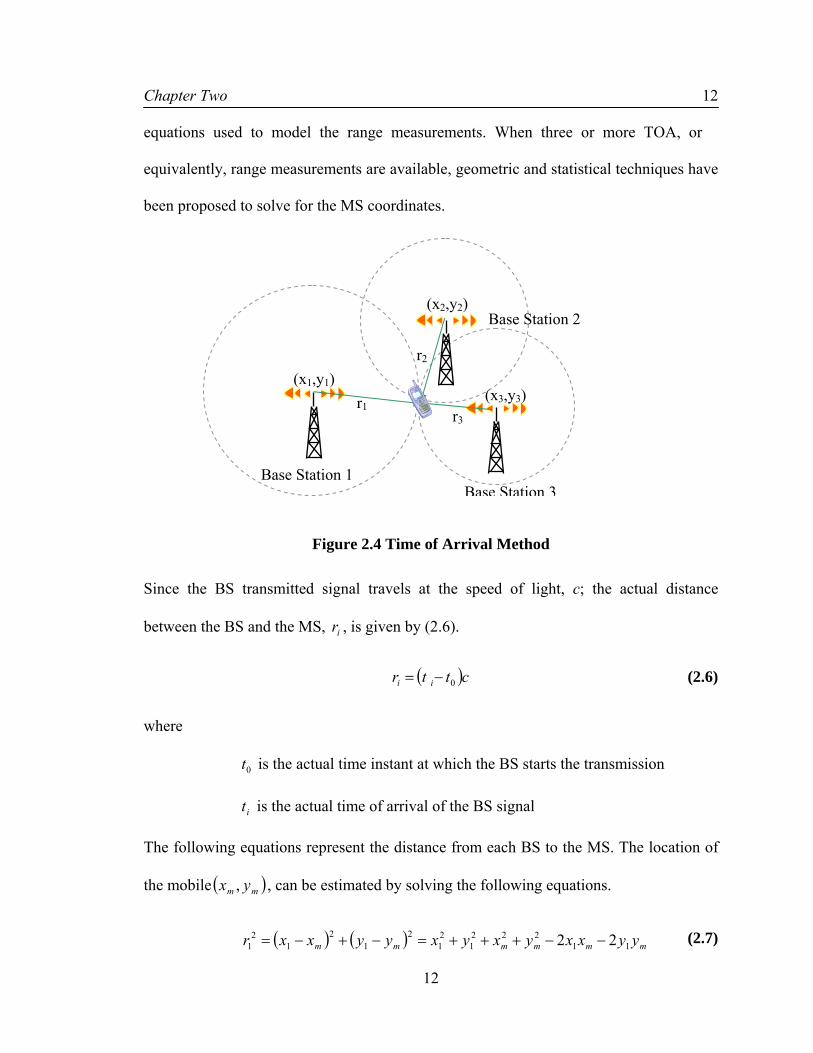
Figure 2.4 Time of Arrival Method
Since the BS transmitted signal travels at the speed of light, c; the actual distance
between the BS and the MS, ir , is given by (2.6).
( )cttr ii 0−= (2.6)
where
0t is the actual time instant at which the BS starts the transmission
it is the actual time of arrival of the BS signal
The following equations represent the distance from each BS to the MS. The location of
the mobile ( )mm yx , , can be estimated by solving the following equations.
( ) ( ) mmmmmm yyxxyxyxyyxxr 11222
121
21
21
21 22 −−+++=−+−= (2.7)
Base Station 3Base Station 1
Base Station 2
(x3,y3)
(x2,y2)
(x1,y1)
r3
r2
r1

Chapter Two
13
13
( ) ( ) mmmmmm yyxxyxyxyyxxr 22222
222
22
22
22 22 −−+++=−+−= (2.8)
( ) ( ) mmmmmm yyxxyxyxyyxxr 33222
323
23
23
23 22 −−+++=−+−= (2.9)
Subtracting (2.7) from (2.8) and (2.7) from (2.9),
( ) ( ) ( ) ( ) mm yyyxxxyxyxrr 121221
21
22
22
21
22 22 −−−−+−+=− (2.10)
( ) ( ) ( ) ( ) mm yyyxxxyxyxrr 131321
21
23
23
21
23 22 −−−−+−+=− (2.11)
Assuming that the BS is located at 01 =x , 01 =y and rearranging terms, the previous two
equations can be written in matrix form as:
( )( ) ⎥
⎦
⎤⎢⎣
⎡
+−++−+
=⎥⎦
⎤⎢⎣
⎡⎥⎦
⎤⎢⎣
⎡2
12
323
23
21
22
22
22
33
22
21
rryxrryx
yx
yxyx
m
m (2.12)
The Least-Square solution is given by (2.13)
( ) BHHH T1-T=⎥⎦
⎤⎢⎣
⎡
m
m
yx
(2.13)
Where, H33
22
=
⎥⎥⎥⎥
⎦
⎤
⎢⎢⎢⎢
⎣
⎡
nn yx
yxyx
MM And
( )( )
( )B
21
21
222
21
23
23
23
21
22
22
22
=
⎥⎥⎥⎥
⎦
⎤
⎢⎢⎢⎢
⎣
⎡
+−+
+−++−+
rryx
rryxrryx
nnn
M
For several BSs (2.13) can be rewritten as
( )( )
( ) ⎥⎥⎥⎥
⎦
⎤
⎢⎢⎢⎢
⎣
⎡
+−+
+−++−+
⎥⎥⎥⎥
⎦
⎤
⎢⎢⎢⎢
⎣
⎡
⎟⎟⎟⎟⎟
⎠
⎞
⎜⎜⎜⎜⎜
⎝
⎛
⎥⎥⎥⎥
⎦
⎤
⎢⎢⎢⎢
⎣
⎡
⎥⎥⎥⎥
⎦
⎤
⎢⎢⎢⎢
⎣
⎡
=⎥⎦
⎤⎢⎣
⎡
−
21
222
21
23
23
23
21
22
22
22
33
22
1
33
22
33
22
21
rryx
rryxrryx
yx
yxyx
yx
yxyx
yx
yxyx
yx
nnn
T
nnnn
T
nn
m
m
MMMMMMM (2.14)

Chapter Two
14
14
2.1.4 Time Difference of Arrival
The Time Difference of Arrival (TDOA) system uses time difference measurements
rather than absolute time measurement as TOA does. In other words, the TDOA approach
uses the differences in the TOA. It is often referred to as the hyperbolic system because
the time difference is converted to a constant distance difference between two base
stations to define a hyperbolic curve. The intersection of two hyperbolas determines the
position. Therefore, it utilizes two pairs of base stations, and at least three for the two-
dimensional case, for positioning [Zhao00].
Figure 2.5 Time Difference of Arrival Method
The following section illustrates how a location solution from TDOA measurements can
be obtained when three BS are involved. The TDOA measurement between BSi and BS1
is defined by,
cttrrr iii )( 111, −=−= (2.15)
Base Station 2
Base Station 3
Base Station 1 d1-d2
d3-d2
Chapter Two
15
15
Note that TDOA measurements are not affected by errors in the MS clock time as it
cancels out when subtracting two TOA measurements [Saye03]. Equation (2.10) can be
rewritten in terms of TDOA measurements as,
( ) ( ) 2122
22
22
211,2 22 ryyxxyxrr mm +−−+=+ (2.16)
Expanding (2.16) and rearranging terms,
( )( )22
22
21,211,222 2
1 yxrrryyxx mm +−+=−− (2.17)
Similarly,
( )( )23
23
21,311,333 2
1 yxrrryyxx mm +−+=−− (2.18)
Rewritten these equations in a matrix form
dpH 1 +=⎥⎦
⎤⎢⎣
⎡ ryx
m
m (2.19)
where
⎥⎥⎥⎥
⎦
⎤
⎢⎢⎢⎢
⎣
⎡
−
−−
=
1,
1,3
1,2
p
nr
rr
M And
⎥⎥⎥⎥⎥
⎦
⎤
⎢⎢⎢⎢⎢
⎣
⎡
−+
−+−+
=
21,
22
21,3
23
23
21,2
22
22
)(
)()(
21d
nnn ryx
ryxryx
M
which yields to the Least-Square solution
( ) ( )dpHHH 1T1T +=⎥
⎦
⎤⎢⎣
⎡ − ryx
m
m (2.20)

Chapter Two
16
16
2.1.5 Hybrid Location Techniques
It is also possible to combine different location techniques to estimate the position of a
MS. These hybrid location techniques are especially useful when the number of available
BS is limited. The surrounding area in which the Mobile Station is located is also critical;
for example TOA has better performance than AOA in urban areas where the antenna
array receives several signals due to multipath. In rural areas, AOA might have better
performance than TOA; this will depend on the quality of the antenna array.
2.2 Non-Line of Sight Conditions
The previous straightforward methods are meant to be used with ideal Line of Sight
(LOS) signals, therefore, when there is no error or a small error in the measurements. If
there is a range error the lines will not intercept in a single point as shown in Figure 2.4,
and this will introduce an error in the estimation of the mobile position.
Unfortunately, in most radio channels, errors in the measured range are frequent and they
are introduced by multipath fading and diffraction effects. Figure 2.6 illustrates this
situation, now the solution is not a unique point; instead the measured ranges define an
area in which the MS can be positioned.
Chapter Two
17
17
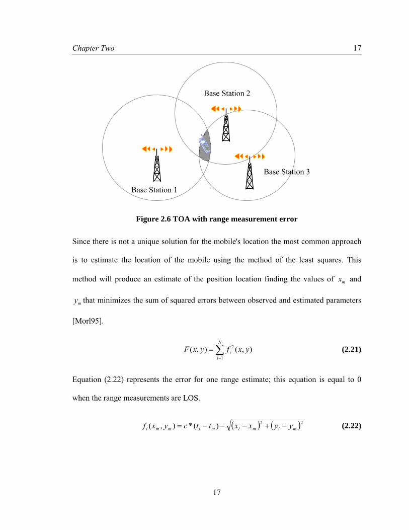
Figure 2.6 TOA with range measurement error
Since there is not a unique solution for the mobile's location the most common approach
is to estimate the location of the mobile using the method of the least squares. This
method will produce an estimate of the position location finding the values of mx and
my that minimizes the sum of squared errors between observed and estimated parameters
[Morl95].
),(),(1
2 yxfyxFN
ii∑
=
= (2.21)
Equation (2.22) represents the error for one range estimate; this equation is equal to 0
when the range measurements are LOS.
( ) ( )22)(*),( mimimimmi yyxxttcyxf −+−−−= (2.22)
Base Station 3
Base Station 2
Base Station 1

Chapter Two
18
18
The aim of the algorithm is to find the minimum point of the bowl-shaped error
surface. Computing the gradient of equation (2.21) will define the direction of the
steepest descendent of the error surface.
[ ] [ ]
[ ] [ ]y
yyxx
yytcyyxx
xyyxx
xxtcyyxxyxF
N
i ii
iiii
N
i ii
iiii
ˆ)()(
**)()(*2
ˆ)()(
**)()(*2),(
122
22
122
22
∑
∑
=
=
−+−
−+−+−
+−+−
−+−+−=∇
(2.23)
The new position estimate is calculated using equation (2.24)
μ*),(),(),( 1 kkk yxFyxyx ∇−=+ (2.24)
where μ is the step size. Iteration starts with an initial value of x and y, in the next
iteration x and y are updated and the iteration continues until the deviation of x and y
becomes negligibly small. It is important that the initial value of x and y are close to the
exact position otherwise the algorithm might not converge
2.3 Sources of Location Error
There are two major sources of error in wireless location systems: Multipath Fading and
Non-Line-of-Sight (NLOS) propagation. Both sources of error are briefly discussed in the
following section.
2.3.1 Multipath Fading
In wireless channels, signals suffer from multiple reflections when traveling from BS to
MS. Fading is caused by the addition of several reflected transmitted signals that reach

Chapter Two
19
19
BS at the same time, each with different amplitude and phase. Based on the phases of
the received signals, they can either add constructively or destructively resulting in fades
as deep as 30 dB when the MS moves only a fraction of a wavelength.
Multipath affects the time-based location systems causing errors in the timing estimates
even when there is a Line-of-Sight (LOS) path between the MS and BS. Delay
estimators, which are based on correlation techniques, are influenced by the presence of
multipath especially when the reflected rays arrive within a chip period of the first
arriving ray [Caff98] since paths separated by a chip period are essentially uncorrelated.
In certain locations the multipath signal may be stronger than the direct path and the
mobile station will report the pilot arrival of the multipath signal instead of the direct
path. As a result, significant mobile positioning error will occur depending on the
reflected path length [Heps99].
2.3.2 NLOS Propagation
As introduced in the previous section, with Non-Line of Sight propagation the signal
arriving at the BS from the MS is reflected or diffracted and takes a longer path than the
direct path. NLOS propagation will bias the TOA or TDOA measurements even when
high-resolution timing techniques are employed and there is no multipath interference.
Therefore, it is important to find methods to mitigate the NLOS error.
The standard deviation of the range measurement is much higher for NLOS than LOS
propagation [Caff98]
Chapter Two
20
20
2.4 Measure of Position Location Accuracy
Several methods have been proposed to evaluate the estimated position accuracy, namely:
• Cramer-Rao Lower Bound (CRLB)
• Circular Error Probability (CEP)
• Geometric Dilution of Precision (GDOP)
The following paragraphs provide a brief definition of these performance measures.
2.4.1 Cramer-Rao Lower Bound
The Cramer-Rao Lower Bound determines that for any unbiased estimator the variance
must be greater than or equal to a given value; thus it can be used as point of reference to
evaluate the performance of the receiver/positioning algorithms. An unbiased estimator is
one that in average will yield the true value of the unknown parameter [Kay98].
If the received signal can be modeled as )(tx , (multipath is not considered)
)()()( 0 ttstx ωτ +−= (2.25)
where
( )ts is the transmitted signal
0τ is the estimated propagation time
( )tω is White Gaussian Noise
It can be shown that the CRLB, expressed in metres, for range estimation is
( )2
0
2
2ˆvar
FN
cRε
≥ (2.26)

Chapter Two
21
21
where
( ) ( )( )∫
∫∞
∞−
∞
∞−=dFFS
dFFSFF
2
22
22π
(2.27)
)(FS is the Fourier transform of )(ts
2F is the mean square bandwidth of the signal
5 10 15 20 25 300
0.5
1
1.5
2
2.5x 10
-3
SNR (dB)
Var
ianc
e R
Figure 2.7 Variance for Range Estimation Error
It is possible to compute the CRLB for Angle of Arrival as well. If the antenna array is
located far from the BS it can be assumed that the incoming signal is a planar wave.
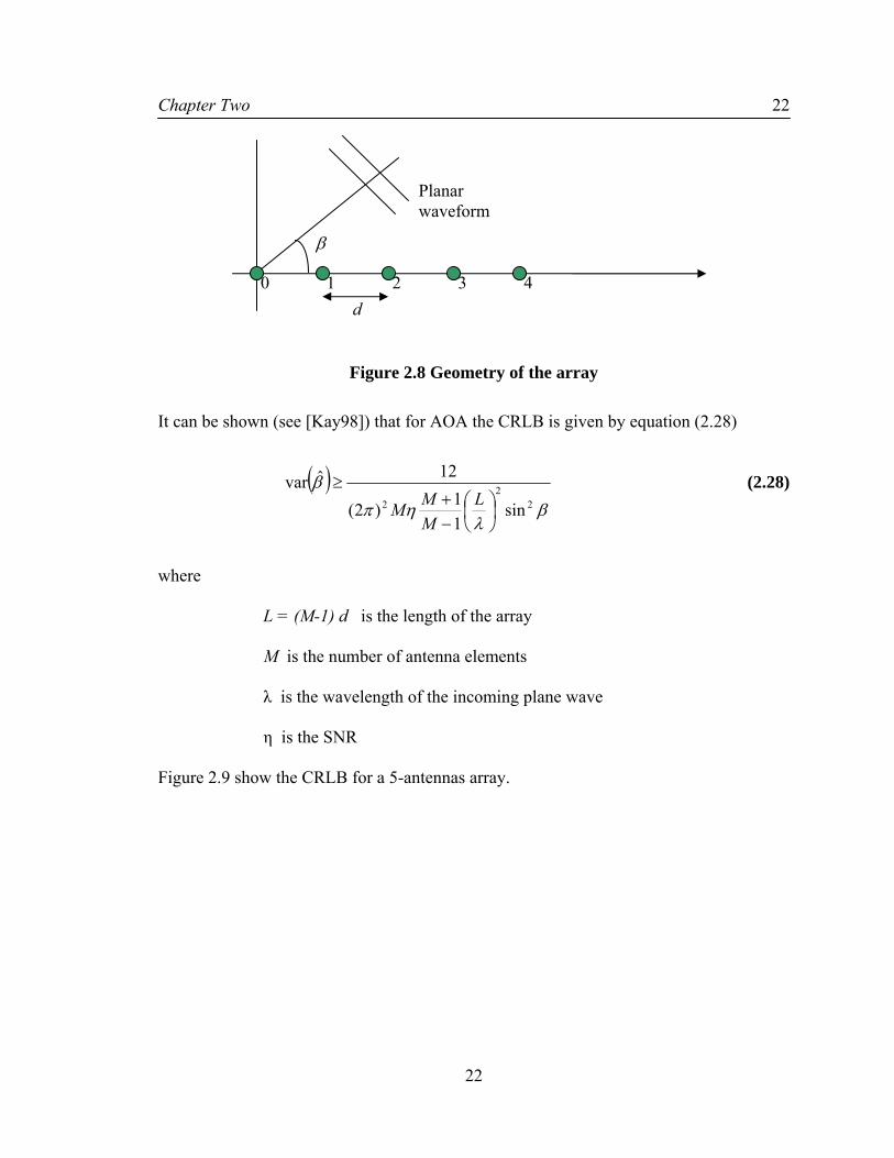
Figure 2.8 shows the array geometry.
Chapter Two
22
22
Figure 2.8 Geometry of the array
It can be shown (see [Kay98]) that for AOA the CRLB is given by equation (2.28)
( )β
ληπ
β2
22 sin
11)2(
12ˆvar
⎟⎠⎞
⎜⎝⎛
−+
≥L
MMM
(2.28)
where
L = (M-1) d is the length of the array
M is the number of antenna elements
λ is the wavelength of the incoming plane wave
η is the SNR
Figure 2.9 show the CRLB for a 5-antennas array.
β
d
1 2 3 4 0
Planar waveform

Chapter Two
23
23
5 10 15 20 25 300.5
1
1.5
2
2.5
3
3.5
4
4.5
5x 10
-4
SNR (dB)
Var
ianc
e β
Figure 2.9 Variance AOA Estimation Error
2.4.2 Circular Error Probability
Circular Error Probability (CEP) is a simple measure of accuracy which is based on the
variance of the position estimates. CEP is defined as the radius of the circle that has its
center at the estimated position and contains half the realization of the location estimates,
as shown in Figure 2.10. In an unbiased estimator, CEP represents the estimator
uncertainty relative to the real MS location. Mathematically, CEP is a complicated
function and is usually approximated; CEP is defined by (2.29)
2275.0 yxCEP σσ +≈ (2.29)
where

Chapter Two
24
24
2xσ is the variance of the position estimate x
2yσ is the variance of position estimate y
As a result, small CEP values indicate high estimator reliability.
Figure 2.10 Circle of Error Probability
2.4.3 Geometric Dilution of Precision
The Geometric Dilution of Precision (GDOP) is defined as the ratio of the Root Mean
Square (RMS) position error to the RMS ranging error. The relative position of the BS
with respect to one another and the MS; has a significant impact on positioning accuracy
[Kluk97]. GDOP is defined by:
s
p
s
yxGDOPσσ
σ
σσ=
+=
22
(2.30)
where
pσ is the standard deviation of the position estimates
sσ is the standard deviation of the ranging error
Mobile Position
Estimated Mobile Position
Bias Vector CEP

Chapter Two
25
25
According to (2.30) a small GDOP value indicates that the error due to a bad geometry
is also small. Therefore, small GDOP is desirable. For testing purposes; the GDOP can be
also used as a criterion for selecting a set of base stations from a large set whose
measurements produce minimum position location’s estimation error.
2.5 Detectability
Detectability is defined as the ability of a CDMA receiver to acquire signals from
multiple Base Stations. It is usually measured in terms of the number of BS that a CDMA
receiver can acquire. With more BS, the receiver can select BS with good geometry and
minimize the DOP. Thus, a high detectability factor (number of Base Stations acquired)
is usually desired. Some of the major factors that affect detectability are,
• BS power control
• Sensitivity of receiver
• Geographical location
The CDMA network uses single frequency reuse which severely limits the transmit
power of a BS. The receiver sensitivity also limits the number of BS that can be acquired.
For example, with a small coherent integration time (defined in Chapter 7), only a small
number of BS can be acquired. On the other hand, using long coherent integration time, a
large number of BS can be acquired.
2.6 Power Control
It is worth to clarify that there are two types of Power Control; the most commonly
referenced Power Control is used because all users transmit on the same frequency and

Chapter Two
26
26
the transmit power for each user must be reduced to limit interference, however, the
power should be enough to maintain the required SNR for a satisfactory call quality.
Additional advantages are longer mobile battery life and longer life span of BS power
amplifiers.
The Power Control that is referenced in this thesis is related to the pilot signal power
level. Since the pilot signal is used to reduce/increase the cell size, variations in the signal
power can be spotted.
Chapter Three
27
27
CHAPTER THREE: THE FORWARD CDMA CHANNEL
3.1 The CDMA Technology Basics
Cellular mobile radio systems aim to provide high-mobility, wide-ranging and two-way
wireless voice communications. This system accomplishes its task by integrating wireless
access with large-scale network, capable of managing mobile users. Cellular radio has
evolved into digital technologies, using the system standards of Global System for
Mobile communications (GSM) at 900 MHz and 1800MHz in Europe, Personal Digital
Cellular (PDC) in Japan.
In the U.S., the initial standards were the Telecommunications Industry Association/
Electronic Industry Association (TIA/EIA) Interim Standard 95 (IS-95), and related
version for versions for base station (IS-97) and mobile performance (IS-98). These
standards define the CDMA system at cellular frequencies (800 MHz Band). Newer
standards from American National Standards Institute (ANSI) defines the performance
for PCS systems (ANSI-J STD-008).The PCS standard differs from IS-95 primarily in
the frequency plan; the basic signal structure are identical.
Code Division Multiple Access (CDMA) is a modulation as well as a multiple-access
technique based on spread-spectrum communication principle. In this scheme, multiple
users share the same frequency band at the same time, by spreading the spectrum of their
transmitted signals, so that each user’s signal is pseudo-orthogonal to the other users. In a
CDMA system, each signal consists of a different binary sequence (called the spreading
code) that modulates a carrier, spreading the spectrum of the spectrum of the waveform.

Chapter Three
28
28
A large number of CDMA signals share the same frequency spectrum. If CDMA is
viewed in either the frequency or time domain, the multiple access signals overlap with
each other. However, the use of statistically orthogonal spreading codes separates the
various signals in the code space.
3.2 Direct Sequence Spread Spectrum
Spread Spectrum communications grew out of research efforts during World War II to
provide secure means of communication, remote control and missile guidance in hostile
environments. This work remained classified until late 1970’s [Vard00].
As introduced in the previous section, a Direct Sequence Spread Spectrum (DSSS)
system spreads the baseband data by directly multiplying the baseband signal with a
pseudo-noise sequence that is produced by a pseudo-noise code generator [Rapp02]. PN
sequences are not random; they are deterministic, periodic sequences. The PN code can
be expressed as:
))1(()(1∑=
−−=N
ncn Tntpdtb (3.1)
where
⎩⎨⎧ ≤≤
=±=otherwise
Tttpd c
n ,00,1
)(,1 (3.2)
and N is the length of the PN sequence.

Chapter Three
29
29
Figure 3.1 Spread Spectrum Encoding
As shown in Figure 3.1; PN code signals are independent of the data, and have a data rate
much higher than that of the desired information. As a consequence, the bandwidth of the
transmitted signal is much larger than the required for transmitting the baseband data.
In Figure 3.1, a(t) is the baseband signal with a bit duration of T, b(t) is the PN sequence
with a chip1 duration of Tc , and A(f) and B(f) are the spectrum of the baseband signal
before and after the dispreading.
A very important parameter of the system is the ratio of transmitted bandwidth to
information bandwidth and is called Processing Gain, pG , of the spread spectrum system.
i
tp B
BG = (3.3)
where,
1 PN sequence’s symbols are called chips
Time-Domain Waveforms
Frequency -Domain Waveforms
b(t)
A(f)
B(f)
a(t)
t
t
f
f
+1
-1
-1
+1
T
Tc
Chapter Three
30
30
tB is the transmission bandwidth
iB is the information bandwidth
As a general comment it can be said that the higher the processing gain is, the higher the
insensitivity to jamming and noise the system becomes.
The advantages of using the Spread Spectrum system are that it provides excellent means
of security while hiding their transmissions in the background noise. As a result, only
those receivers that have knowledge of the transmitted PN sequence can recover the user
message. Furthermore, it provides resistance against narrowband interference within the
bandwidth of the signal since the decorrelation process used to despread the received
signal at the receiver, spreads the energy of the narrowband interference signal over a
large bandwidth.
3.3 The Forward CDMA Channel
The forward CDMA link or downlink is composed of the pilot channel, sync channel,
paging channel and traffic channel. Each of these channels is orthogonally spread by the
appropriate Walsh function and is then spread by a quadrature pair of PN sequences. The
purpose of each channel is described in the next sections.
3.3.1 The Pilot Channel
The Pilot Channel serves as a coherent phase reference for demodulating the other
channels [Yaco02]. Further analysis of the Pilot Channel is carried out in the next section
of this chapter.

Chapter Three
31
31
3.3.2 The Synchronisation Channel
The Synchronisation Channel provides the information required to allow communication
between the Base Station and the Mobile Station and operates at a fixed rate of 1200 bps.
This signal also identifies the particular transmitting base station [Lee98]. There is one
synchronization channel per cell. The Synchronization Channel is assigned Walsh code
32.
3.3.3 The Paging Channel
The paging channel carries paging messages between the BS and the MS; in addition this
channel carries general system information as handover thresholds, maximum number of
unsuccessful attempts, a list of the surrounding cells and channel assignment messages
[Steel01]. There can be up to seven paging channels per CDMA carrier and they operate
at 9600 or 4800 bps. The Paging Channel is assigned Walsh code 1 to 7.
3.3.4 The Traffic Channel
There are up to 55 forward Traffic Channels that carry the digital voice or data to the
mobile user [Lee98]. The base station may transmit information at the different rates of
9600, 4800, 2400, and 1200 bps. The Walsh codes designated for the Traffic channel are
from 8 to 31 and from 33 to 63.
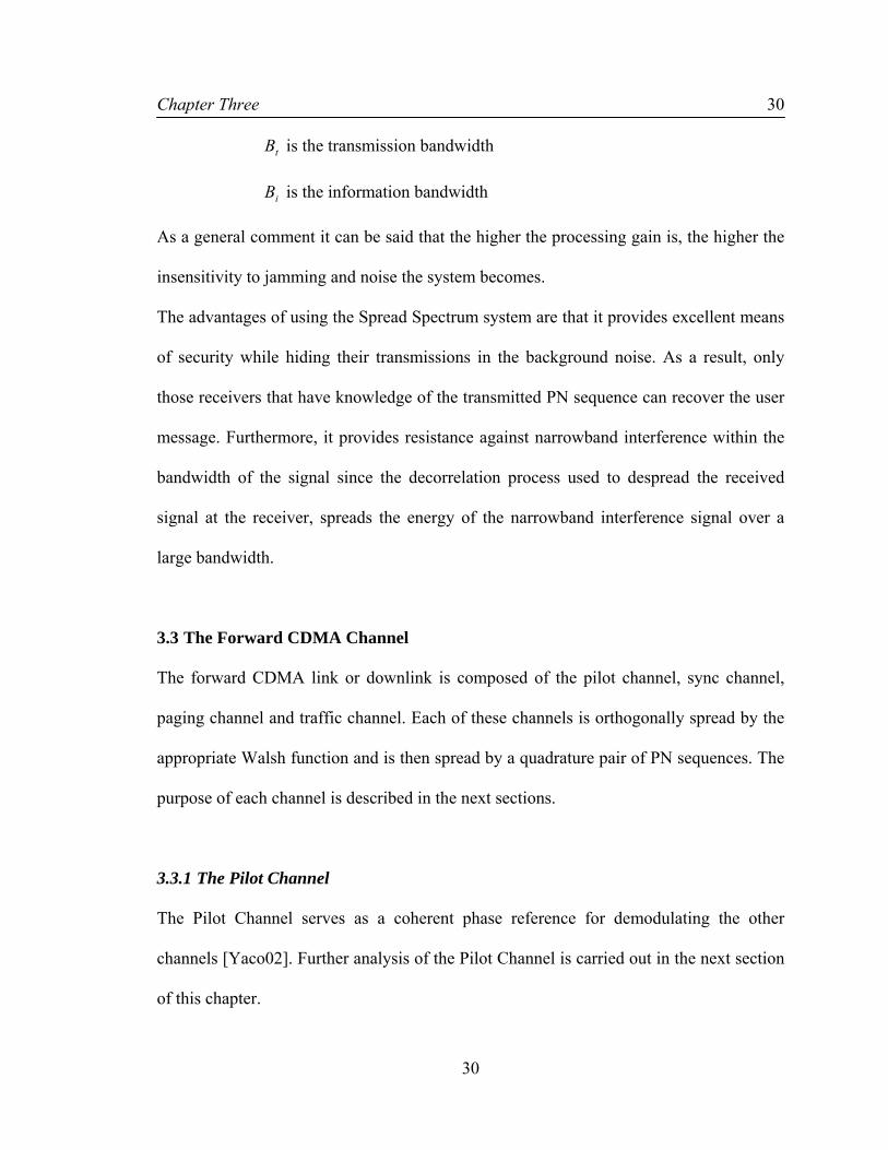
3.4 The Pilot Channel
The Pilot Channel has no data modulation (therefore, it is easily acquired by the Mobile
Station), it only has the in-phase and quadrature phase Pseudorandom Noise (PN) codes
Chapter Three
32
32
are transmitted; this PN code is used to spread the spectrum. The sample rate of the
spreading sequence (called chip rate) is chosen so that the bandwidth of the filtered signal
is several times the bandwidth of the original signal. The Pilot Channel is used to achieve
initial system synchronization and also provide robust time, frequency and phase tracking
of the signal transmitted by the BS [Rhee98]. The Pilot Channel transmitted power level
for all base stations is 4-6 dB higher than a traffic channel with a constant value
[Garg97].
Figure 3.2 Pilot Channel Structure
This channel is transmitted continuously by the BS and tracked all the time by the MS.
Since the transmitted power level of this channel can be modified, the Pilot Channel is
used to modify the covered area of the cell.
Baseband Filter
Baseband Filter
All 0’s
)sin( 0tω
I-channel pilot PN chips 1.2288 Mcps
Walsh Function 0
)cos( 0tω
Q-channel pilot PN chips 1.2288 Mcps
I(t)
Q(t)

Chapter Three
33
33
3.5 Walsh Function
Each channel in the CDMA forward link is spread with Walsh function at a fixed chip
rate of 1.2288 Mcps. The Walsh functions consist of sixty-four binary sequences, each of
length 64, which are completely orthogonal to each other and provide orthogonal
channelization for all users. The Walsh function repeats every 52.083 µs, which is equal
to one coded data symbol (Code Data Rate 19200 bps) [Rapp02]. The 64 by 64 Walsh
function is generated by the following recursive procedure.
01 =H ⎥⎦
⎤⎢⎣
⎡=
1000
2H
⎥⎥⎥⎥
⎦
⎤
⎢⎢⎢⎢
⎣
⎡
=
0110110010100000
4H ⎥⎦
⎤⎢⎣
⎡=
NN
NNN HH
HHH 2 (3.4)
where N is a power of 2. Each code of the Walsh function matrix corresponds to a
channel. The Pilot Channel is assigned Walsh code 0, which is the all zeros code, then the
pilot channel is nothing more than a blank Walsh code and thus consist only of the
quadrature PN spreading code.
3.6 Quadrature Spreading
The two distinct short PN codes in Figure 3.2 are maximal length sequences generated by
combining the outputs of the feedback of the 15-stage shift registers and lengthened by
the insertion of one chip per period in a specific location in the PN sequence. Thus, these
modified short PN codes have periods equal to the normal sequence length of 215-
1=32,767 plus one chip, or 32,768 chips.

Chapter Three
34
34
A feedback shift register consist of consecutive two-state memory and feedback logic.
Clock pulses are used to shift Binary sequence through the shift register. The contents of
the stages are logically combined to produce the input to the first stage. The initial
contents of the stages and feedback logic determine the successive contents of the stages
[Garg97]. A linear feedback shift register is shown in Figure 3.3.
Figure 3.3 Block Diagram of a linear feedback shift register
The connections between different stages are defined by the characteristic polynomials.
The characteristic polynomials of the in-phase and quadrature sequence are given by
(3.5) and (3.6) respectively.
151398751)( xxxxxxxPI ++++++= (3.5)
1512111065431)( xxxxxxxxxPQ ++++++++= (3.6)
Based on the characteristic polynomials, the pilot PN sequences i(n) and q(n) are
generated by the following linear recursions:
)2()6()7()8()10()15()( −⊕−⊕−⊕−⊕−⊕−= ninininininini (3.7)
Feedback Logic
Stage 1
Stage 2
Stage 3
Stage 4
Stage 15
Clock
Chapter Three
35
35
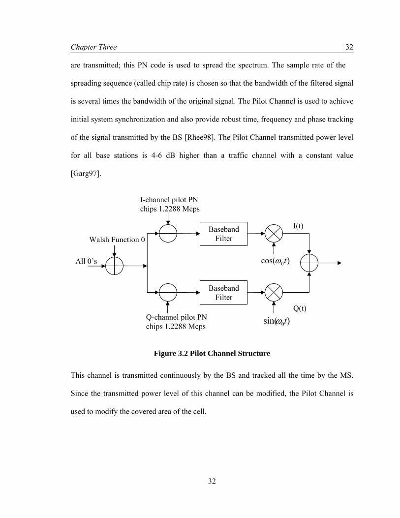
)3()4()5()9()10()11()13()15()(
−⊕−⊕−⊕−⊕−⊕−⊕−⊕−=
nqnqnqnqnqnqnqnqnq
(3.8)
where i(n) and q(n) for 767,321 ≤≤ n represent binary value 0 or 1, and i(15)=1 and
q(15)=1, and ⊕ represents modulo-2 addition also known as exclusive OR. The Pilot
PN sequences are obtained by inserting an extra 0 after 14 consecutives 0’s in the PN
sequences i(n) and q(n). Thus, each pilot PN sequences has exactly one run of 15
consecutives 0’s and one run of 15 consecutives 1’s. The extra 0 is inserted so that there
are an integer number of periods of the Walsh code functions for every period of the PN
sequence [Blan98].
As indicated previously each Base Station is distinguished by a different phase offset of
the in-phase and quadrature-phase PN sequences. Each offset is a multiple of 64 PN
chips, which yields 32,768/64=512 possible 64-chip offsets.
3.7 Baseband Filtering
Following the quadrature spreading operation the I and Q data are applied to the
baseband filters as described in Figure 3.2. When rectangular pulses are passed through a
band limited channel, the pulses will spread in time, and the pulse for each symbol will
smear into the time intervals of succeeding symbols [Rapp02]. This causes Intersymbol
Interference (ISI) which leads to an increased probability of error when detecting a
symbol in the receiver.
In order to reduce ISI a 48-tap finite impulse response (FIR) pulse shaping filter is used;
the coefficients for this filter are provided by the CDMA standard.

Chapter Three
36
36
The baseband filters shall have a frequency response S (f) that satisfies the limits given
in Figure 3.4.
Figure 3.4 Baseband Filters Frequency Response
The limits of the normalized frequency response of the filter shall be contained within
±δ1 in the passband 0≤ f≤ fp and the normalized response in the stopband; f≤ fs; should be
less than –δ2. The numerical values for these parameters are δ1=1.5 dB, δ2=40 dB, fp=590
kHz and fs=740 kHz.
3.8 Quadrature Phase Shift Keying (QPSK).
The CDMA signal is sometimes mistakenly believed to employ QPSK modulation. In
classical QPSK the information stream is split, with half transmitted over the I channel
and half transmitted over the Q channel. In the forward link signal described in this
chapter, however, all the information is transmitted over both channels. Therefore, the
δ 2
δ 1
fp fs
0
20 log10 S(f)
f
0

Chapter Three
37
37
signal is not truly a QPSK signal, but rather Binary Phase Shift Keying (BPSK) on
quadrature channels. Transmitting all the data over both channels is a diversity scheme,
since the decision-making in the receiver has the option of using the information from
two demodulated information streams rather than one [Blank98]. An orthogonal QPSK
waveform s(t) (3.9) is obtained by amplitude modulation of I(t) and Q(t) each onto the
cosine and sine functions of a carrier wave. The in-phase stream I(t) amplitude-modulates
the cosine function with an amplitude of +1 or -1, produces a BPSK wave form; whereas
the quadrature-phase stream Q(t) modulates the sine function, resulting in a BPSK
waveform orthogonal to the cosine function.
))(cos(2)(
)sin()()cos()()(
0
00
ttts
ttQttIts
θω
ωω
−=
+=(3.9)
where )()(tan)())(sin(2)())(cos(2)( 1
tItQtttQttI −=== θθθ
The resulting constellation and phase transition is shown in Figure 3.5
Figure 3.5 Forward CDMA channel signal constellation and phase transition
Q-Channel
(0, 1)
(1, 0)
(1, 1)
(0, 0)
I-Channel

Chapter Three
38
38
3.9 Frequency and Channel Specification
The IS-95A CDMA system is specified for reverse link operation in the 829 – 849 MHz
band and the forward link operation in the 869 – 894 MHz band. The PCS version of IS-
95A operates in the 1800 – 2000 MHz band. The forward link is allocated to the higher
frequency range compared to the reverse link. Table 3-1 summarizes the channel
assignment adopted in the PCS band.
Table 3-1 PCS Band Channel Assignment
Band Frequency (MHz) Channel Numbers
Reverse Link 1850 + 0.05N 12000 ≤≤ N
Forward Link 1930 + 0.05N 12000 ≤≤ N
In Table 3-1, N is the channel number. For example, N=350 correspond to a CDMA
channel with a carrier frequency of 1867.5 MHz. Figure 3.6 shows the channel
assignment in an IS-95A CDMA system in the PCS band. These CDMA cannels are
grouped in blocks of 5 MHz or 15 MHz band and occupy a discrete part of the PCS
spectrum.

Chapter Three
39
39
Figure 3.6 CDMA Channel Assignment
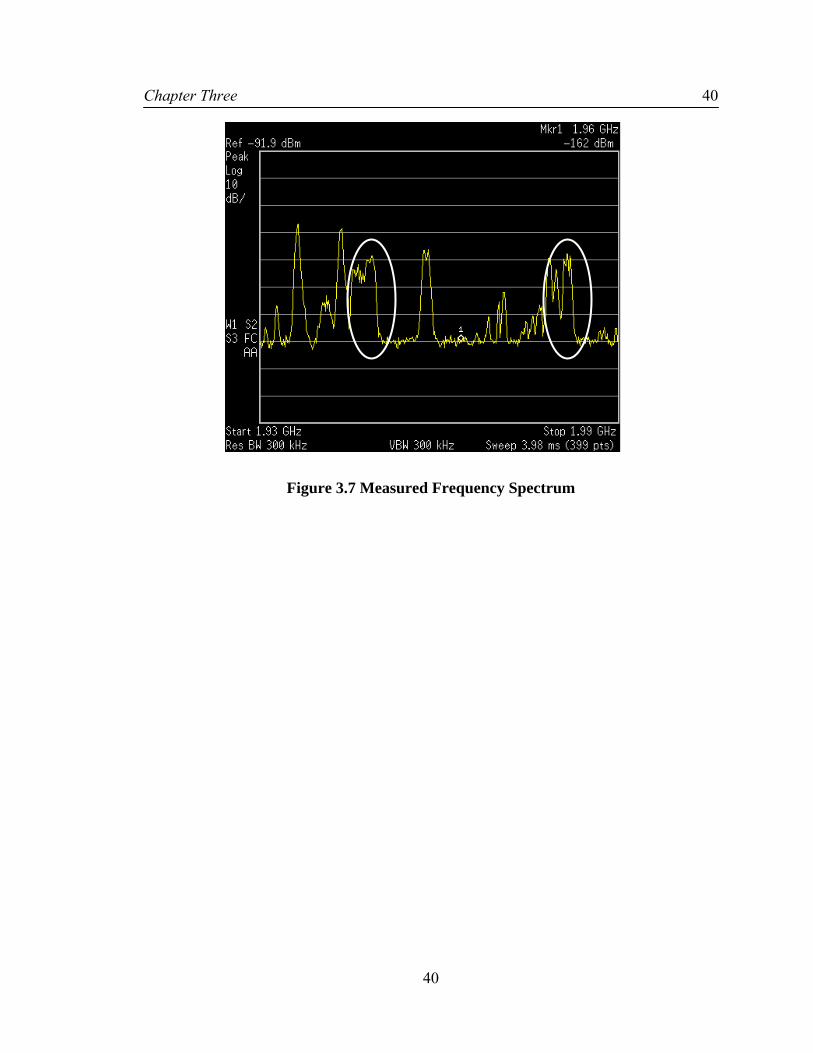
Figure 3.7 shows the measured, on air, frequency spectrum at the University of Calgary
using a spectrum analyzer. The signal was passed through a Low Noise Amplifier (LNA)
prior to spectrum measurement. In the Figure 3.7, a 5MHz (Block D) CDMA channel is
highlighted. The 5 MHz multi-carrier band is usually adopted to increase the capacity of
the resulting CDMA system.
These carriers are orthogonal to each other and the readers are referred to [TIA/EIA00]
for more details. Block D corresponds to channel numbers 300 to 399. A second CDMA
channel was found in Block C of the PCS band. Block C corresponds to channels 900 to
1199.
1945 1947.5
50 kHz
2.5 MHz
1.25 MHz
1.2 MHz
1946.2
Chapter Three
40
40
Figure 3.7 Measured Frequency Spectrum

Chapter Four
41
41
CHAPTER FOUR: RECEIVER STRUCTURE
4.1 Receiver Structure
As introduced beforehand, the objective of this receiver development is to investigate the
use of CDMA pilot signal emanating from commercial PCS band wireless network for
positioning of a mobile. To facilitate this, a specialized PCS downlink receiver needs to
be implemented that will support Time of Arrival measurements with sufficient degree of
accuracy.
Special considerations have to be taken into account since the designed receiver will be
used not only for TOA measurements but also for AOA measurements. The accuracy of
the receiver will depend on the signal bandwidth, the antenna element spacing (for AOA
measurements) and the quality of the receiver hardware.
In order to have a highly accurate receiver it is crucial that the signal received at each
antenna is amplified, filtered, downconverted and sampled in an identical manner
[Rapp96]. This means that every channel in the receiver must have virtually the same
Impulse Response, be highly linear, and share the same oscillators to downconvert and
sample the received signal.
Since a high level of integration was not the primary objective in the receiver design,
different receiver architectures were studied in order to design a receiver with good
performance in terms of selectivity and sensitivity. Based on this objective, a 5-channel
receiver as shown in Figure 4.1 is developed and used to support this project.
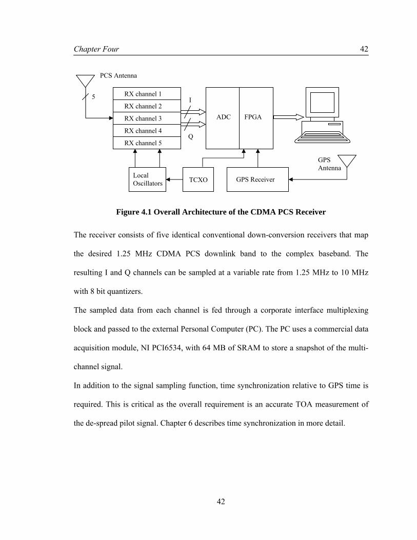
Chapter Four
42
42
Figure 4.1 Overall Architecture of the CDMA PCS Receiver
The receiver consists of five identical conventional down-conversion receivers that map
the desired 1.25 MHz CDMA PCS downlink band to the complex baseband. The
resulting I and Q channels can be sampled at a variable rate from 1.25 MHz to 10 MHz
with 8 bit quantizers.
The sampled data from each channel is fed through a corporate interface multiplexing
block and passed to the external Personal Computer (PC). The PC uses a commercial data
acquisition module, NI PCI6534, with 64 MB of SRAM to store a snapshot of the multi-
channel signal.
In addition to the signal sampling function, time synchronization relative to GPS time is
required. This is critical as the overall requirement is an accurate TOA measurement of
the de-spread pilot signal. Chapter 6 describes time synchronization in more detail.
RX channel 1
RX channel 2
RX channel 3
RX channel 4
RX channel 5
GPS Receiver
ADC FPGA
TCXO Local Oscillators
Q
I 5
PCS Antenna
GPS Antenna

Chapter Four
43
43
4.2 Alternative Receiver Architectures
In this section different receiver architectures are described in detail. This section also
reviews the radio receiver by presenting their different features which characterize any
particular digital receiver architecture.
4.2.1 Superheterodyne Receiver
Most RF communication transceivers manufactured today utilize some variant of the
conventional superheterodyne approach [Rude97]. In this system, the receiver is
implemented with a collection of discrete-components filters and various technologies
such as GaAs silicon bipolar and CMOS [Gray95]. The essential components of modern
single conversion superheterodyne receiver architecture are shown in Figure 4.2.
Figure 4.2 Conventional Superheterodyne Receiver Architecture
One advantage of having one or more stages like in the superheterodyne receiver is gain
distribution. If a large gain is required prior to the circuits which extracts the baseband
information, then it is best for this gain to be distributed over several stages. With a large
A/D
LO 1
Post LNA Filter
LNA
Input RF Filter
Mixer IF Amp
IF Filter
Baseband Filters
LO 2
Antenna
900
Demodulator

Chapter Four
44
44
gain at a single frequency, practical amplifiers are prone to oscillate, since small
amounts of feedback are inevitable.
It is usually better to reduce the gain at each frequency and distribute the gain over
several stages to reduce the tendency of the amplifiers to oscillate. Making filtering easier
is another advantage of having multiple IF stages. High frequency filters with narrow
bandwidths are very difficult to construct and very expensive also. The solution is to
translate the signal to a lower frequency band where the bandwidth required is a larger
fraction of the center frequency; therefore filters are easier to construct [Blank98].
Another important characteristic is that the superheterodyne receiver can offer excellent
sensitivity and selectivity [Sun04].
The main disadvantage of having multiple IF stages is that the cost of the receiver is
higher due to the increased number of parts as passive filters and additional oscillator,
these components also require extra housing space. The increased number of parts also
results in higher power consumption in the receiver. Another disadvantage is that this
architecture tends to rely heavily on the use of Automatic Gain Control.
4.2.2 Homodyne Receiver
The motivation behind eliminating off-chip components has led to zero-IF receiver
architectures [Meht01]. A receiver architecture that eliminates many off-chip components
in the receiver signal path is the direct conversion or homodyne architecture.
A direct conversion receiver architecture eliminates the IF stage as well as the need for
image rejection filtering [Rude98]. Figure 4.3 shows a block diagram for a conventional
homodyne receiver.

Chapter Four
45
45
Figure 4.3 Conventional Homodyne Receiver’s Architecture
In a homodyne receiver, the received signal is passed through an RF filter which is used
to improve dynamic range by rejecting potentially large out-of-band interferers
[Kuhn95]. The portion of the spectrum passed through the filter is then amplified and
mixed with a local oscillator equal to the frequency of the desired signal; in this way, the
desired channel is selected by tuning the frequency of the local oscillator to match the
incoming carrier frequency. This converts the signal directly to baseband were final
channel select filtering is performed. In consequence direct conversion receiver requires
tighter centering of the LO frequency.
There are some limitations to the performance of the direct conversion receiver; these
include the 1/f noise from the amplifier and mixer (1/f noise is a low-frequency noise
whose power density decays with the inverse of frequency; this noise is generated by
impurities within the semiconductor). Another source of interference arises from DC
offsets and DC products resulting from second-order nonlinear distortion in the amplifier
and mixer [Bess03II].
LNA
RF Filter
Demodulator A/D
Baseband Filters
LO
900
Chapter Four
46
46
Superheterodyne receivers can deal with DC offset better than homodyne receivers
because the DC offset can easily be filtered out at the first IF without any loss of
information; it is not possible to eliminate the DC offset in homodyne receivers without
losing information.
4.2.3 Low-IF Receivers
Most of the benefits of homodyne receivers increase if the IF is translated to a low but
nonzero value instead of to DC as in homodyne receivers [Gray95]. The structure of this
receiver is similar to the direct conversion receiver; Figure 4.3; a single mixer is used to
translate the signal into an IF frequency; this IF frequency is typically on the order of one
or two channels bandwidth.
The primary advantage of a low-IF system is that the desired channel is offset from DC.
Therefore, the typical problems arising from DC offsets found in direct-conversion
receivers may be bypassed [Rude98].
4.3 Receiver Front-End
A receiver front end, as seen in the previous section, needs to achieve different
objectives: amplification, filtering, mixing and demodulation. A single-conversion
superheterodyne architecture was the selected receiver structural design; since low-power
consumption and highly integrated schemes were not the objectives of this work.
The design of superheterodyne receiver involves many trade-off including selection of
Intermediate Frequency and Local Oscillators frequencies to meet image rejection and
spurious responses objectives. The receiver structure is illustrated in Figure 4.5; the RF

Chapter Four
47
47
LO converts the incoming signal first to an IF at a relatively high frequency, and then
the IF LO converts the IF signal into baseband.
The following sections are dedicated to explain how each component of the developed
receiver works and influences the functioning of the entire receiver.
Figure 4.4 Picture of the developed receiver

Chapter Four
48
Figure 4.5 Superheterodyne Receiver Block Diagram (Single Channel)
Pow
er
Det
ecto
r R
F LO
IF
LO
Ant
enna
IF V
GA
IF F
ilter
Pow
er
Det
ecto
r
Dem
odul
ator
V
GA
Post
LN
A
Filte
r
LNA
In
put R
F Fi
lter
Mix
er
Buf
fers
Bas
eban
d Fi
lters
90
0

Chapter Four
49
4.3.1 Input RF Filter
The input RF filter or pre-selector filter (since it selects only the receive band) has the
precise function of preventing the out-of-band signal from entering a subsequent section
and saturating the initial stages. However, the RF filter provides no protection against
third-order intermodulation distortion produced by “in-band” signals. In order to keep
the noise figure as low as possible the selected input RF filter has a low insertion loss.
Table 4-1 RF Filter Parameters
Parameter Typical Value
Center Frequency 1960 MHz
Bandwidth 60 MHz
Insertion Loss 2.1 dB
Max. RF Input Power 13 dBm
The filter selected for this stage is a Surface-Acoustic-Wave (SAW) filter (855817 from
SAWTEK). Acoustic filters such as SAW filters converts electrical energy to mechanical
vibrations, process the signal acoustically, and then convert the energy back to an
electrical form. The equations describing a mechanically vibrating resonator, where
energy is cycled between kinetic motion and stress, match those of an inductor and
capacitor (LC) attached in parallel, where energy is cycled between the electric field of
the capacitor and the magnetic field of the inductor. However, the mechanical resonators
have much higher Q's and better stability than the LC circuit.
Table 4-1 tabulates the filter characteristics. Figure 4.6 shows the RF filter frequency
response.
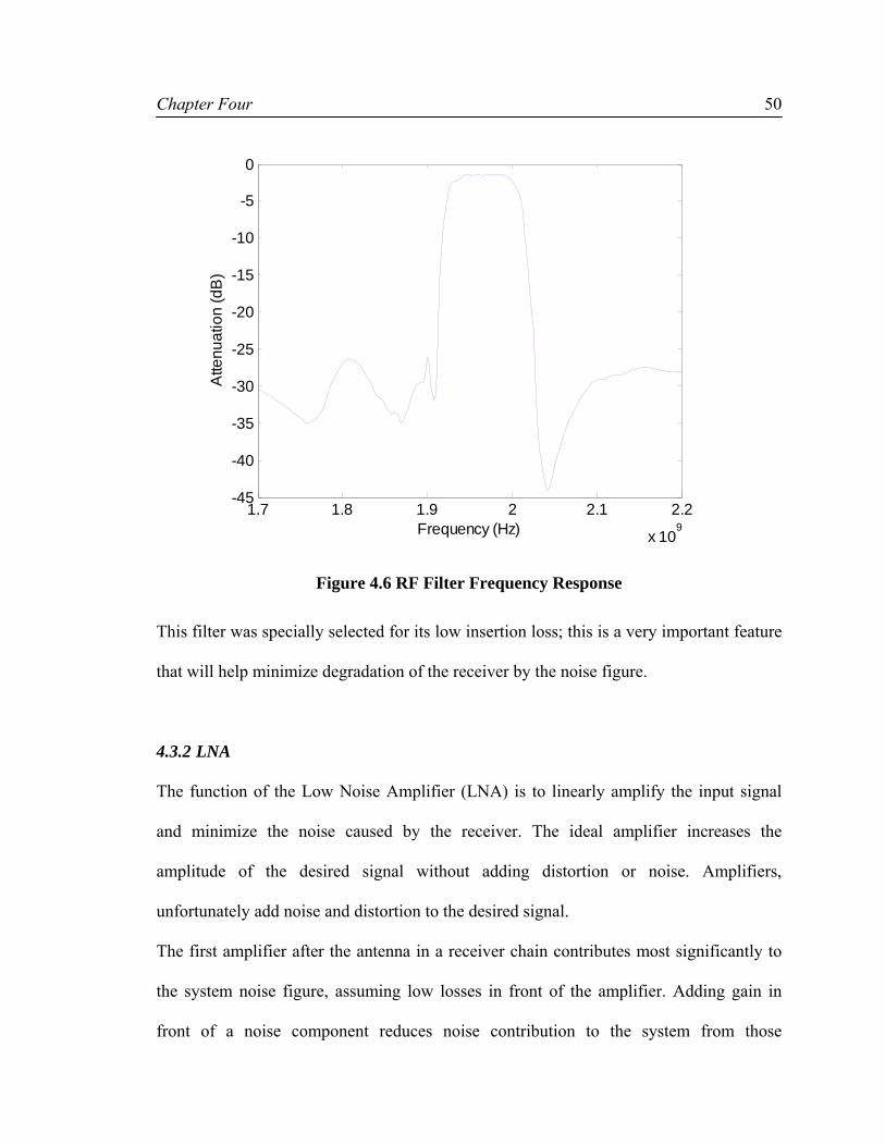
Chapter Four
50
1.7 1.8 1.9 2 2.1 2.2
x 109
-45
-40
-35
-30
-25
-20
-15
-10
-5
0
Frequency (Hz)
Atte
nuat
ion
(dB
)
Figure 4.6 RF Filter Frequency Response
This filter was specially selected for its low insertion loss; this is a very important feature
that will help minimize degradation of the receiver by the noise figure.
4.3.2 LNA
The function of the Low Noise Amplifier (LNA) is to linearly amplify the input signal
and minimize the noise caused by the receiver. The ideal amplifier increases the
amplitude of the desired signal without adding distortion or noise. Amplifiers,
unfortunately add noise and distortion to the desired signal.
The first amplifier after the antenna in a receiver chain contributes most significantly to
the system noise figure, assuming low losses in front of the amplifier. Adding gain in
front of a noise component reduces noise contribution to the system from those

Chapter Four
51
components. Subsequent stages have less and less influence on the overall noise figure
of the system. Increasing gain from the low-noise amplifier improves the system noise
figure.
The LNA must provide good linearity, because it is possible that the desired signal may
be accompanied by stronger interfering signals elsewhere in the receiver band. If the
LNA is not sufficiently linear, these stronger signals could generate inter-modulation
responses that coincide exactly with the desired signal, and will not be removed by any
other of the later components [Bess03].
The AM50-0012 manufactured by MA-COM, the LNA selected for this receiver, is
ideally suited to be used where low noise figure, high gain, and high dynamic range are
required. This LNA requires an external input matching network.
Table 4-2 LNA Specifications
Parameter Typical Value
Gain 19 dB
Noise Figure 1.4 dB
Input IP3 13 dBm
Supply Voltage 5 Volts
Drain Current 80 mA Table 4-2 shows the specification of this critical component which will define the overall
receiver noise figure.

Chapter Four
52
4.3.3 Post LNA Filter
The Low Noise Amplifier will provide gain to all channels within the RF bandwidth, and
its gain is likely to roll off beyond it. The amplifier will also amplify noise across the
entire band, and possibly any signal at the image frequency as well.
Therefore, the post-LNA filter is used to suppress any gain of undesired signal responses
at spurious frequencies, and in particular at the image frequency. The filter used at this
stage is the 855817 from SAWTEK, same as the input filter.
4.3.4 Linear Variable Gain Amplifier
CDMA receivers must often be capable of handling a signal range of 80 dB or more.
Most amplifiers remain linear over only a much smaller range. Therefore, an Automatic
Gain Control is needed to prevent overload or inter-modulation of the subsequent stages
and to adjust the input mixer level for optimum operation.
The RF2377 is a linear variable gain amplifier selected for power control in the RF stage,
a full closed loop is implemented by using the AD8313 Logarithmic Detector at the
output of the amplifier. Table 4-3 shows the VGA specifications.
Table 4-3 RF Variable Gain Amplifier Specifications
Parameter Typical value
Usable Frequency 800 to 2100 MHz
Linear Gain Control Range 50 dB
Noise Figure 9 dB (Max. Gain)
Input IP3 6 dBm
Gain Control Slope 70 dB/V
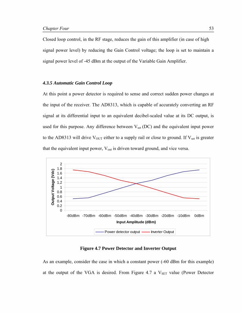
Chapter Four
53
Closed loop control, in the RF stage, reduces the gain of this amplifier (in case of high
signal power level) by reducing the Gain Control voltage; the loop is set to maintain a
signal power level of -45 dBm at the output of the Variable Gain Amplifier.
4.3.5 Automatic Gain Control Loop
At this point a power detector is required to sense and correct sudden power changes at
the input of the receiver. The AD8313, which is capable of accurately converting an RF
signal at its differential input to an equivalent decibel-scaled value at its DC output, is
used for this purpose. Any difference between Vset (DC) and the equivalent input power
to the AD8313 will drive VOUT either to a supply rail or close to ground. If Vset is greater
that the equivalent input power, Vout is driven toward ground, and vice versa.
00.20.40.60.8
11.21.41.61.8
2
-80dBm -70dBm -60dBm -50dBm -40dBm -30dBm -20dBm -10dBm 0dBm
Input Amplitude (dBm)
Out
put V
olta
ge (V
dc)
Power detector output Inverter Output
Figure 4.7 Power Detector and Inverter Output
As an example, consider the case in which a constant power (-60 dBm for this example)
at the output of the VGA is desired. From Figure 4.7 a VSET value (Power Detector

Chapter Four
54
Output Curve) of ~0.75 V is required to maintain the VGA output power at a constant -
60 dBm. As stated previously, if the equivalent input power to the AD8313 is less than
VSET, VOUT will be driven toward ground. This is not acceptable when there is a low input
signal power; because an increase in the gain in VGA is required. As a result, an inverter
circuit at the output of the AD8313 is used in order to change the sign of the slope.
Figure 4.7 shows the input to the VGA (red curve).
Figure 4.8 Block Diagram of the AGC Loop
The AGC has a delay in its response to an input. This means that the AGC control
voltage holds constant for a short time after a change in signal level and then follows the
change to compensate for the level change. In practice, it is not desirable for an AGC to
have too fast a reaction time. In such a case, any static pulse, ignition noise or other
impulsive interference with very fast rise time would be detected by the AGC detector
and would desensitize the receiver or modulate the amplitude of the received signal.
Selection of the proper AGC time constant is a subjective decision. Most receiver
manufacturers now set the attack time between 20 and 50 ms. However, the attack time
selected for the developed receiver was 15 ms, this time is defined by an RC filter placed
at the output of the inverter.
AD8313
Vout
AD8041
Vset
1.1V
RF2377
+
- RFIN

Chapter Four
55
4.3.6 Mixer
The mixer is one of the fundamental blocks of a wireless communication system; the
primary function of the mixer is to translate an RF frequency into lower intermediate
frequency (210.38 MHz in this particular design) preserving phase information within the
new range of frequencies.
An important aspect of the mixer is the selection of the Intermediate Frequency. The
selected frequency for IF and Local Oscillators were determined after detailed study of
spurious mixing products, harmonic interference and availability of components for the
selected frequencies.
Table 4-4 Mixer Specifications
Parameter Typical Value
Usable Frequency (LO) 200 to 3000 MHz
Usable Frequency (RF) 200 to 3000 MHz
Usable Frequency (IF) 0 to 1000 MHz
RF Power (Max.) 1 dBm
Conversion Loss (Max.) 9 dB
Input IP3 14 dBm
LO Power 7 dBm
Table 4-4 shows the specification of the double balanced mixer (ADE-30 from
Minicircuits) used in the developed receiver. A double balanced mixer topology was
selected in order to reject certain unwanted mixer output components. The double
balanced mixer with balanced diodes and transformers cancels the even harmonics of
both the RF and LO frequencies and provides isolation among the various ports. The

Chapter Four
56
mixer is the dominant source of intermodulation distortion [Chan01], a trade-off
between the amplifier gain and noise figure characteristics with those of mixer was
required for the design of this receiver.
4.3.7 IF Filter
An IF filter allows only an IF frequency to pass to the demodulation circuitry rejecting
the image frequency, the local oscillator feed-through and undesired mixing products. In
the developed receiver, a narrowband SAW filter following the mixer is used to reject the
adjacent channel. This keeps receiver selectivity as high as possible close to the antenna,
and can prevent propagation of unwanted signals further downstream.
2.05 2.1 2.15
x 108
-80
-70
-60
-50
-40
-30
-20
-10
Frequency (Hz)
Atte
nuat
ion
(dB
)
Figure 4.9 IF Filter Frequency Response

Chapter Four
57
Figure 4.9 shows the frequency response of the selected IF filter and Table 4-5 list the
parameters of the selected SAW filter.
Table 4-5 IF Filter Specifications
Parameter Typical Value
Center Frequency 210.38 MHz
Bandwidth 1.26 MHz
Insertion Loss 7.2 dB
System noise bandwidth is defined by the IF filter; the system noise bandwidth is key in
determining a receiver’s sensitivity level.
4.3.8 IF Variable Gain Amplifier
In the IF stage, another VGA is used in order to achieve a Dynamic Range of around 80
dB. The IF amplifier provides the necessary gain to boost the IF signal to a level required
by the detector or to an additional down-conversion stage. IF amplifier stages have less
effect on the overall receiver noise figure although dynamic-range characteristics are
important to receiver performance. However, interfering signals are usually greatly
reduced by the IF filter, making the second-order and third-order intercept point
requirements of the IF amplifier minimal.
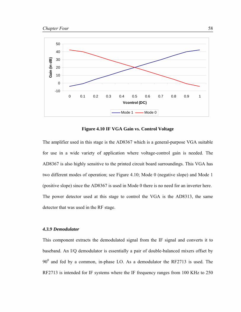
Chapter Four
58
-10
0
10
20
30
40
50
0 0.1 0.2 0.3 0.4 0.5 0.6 0.7 0.8 0.9 1
Vcontrol (DC)
Gai
n (in
dB
)
Mode 1 Mode 0
Figure 4.10 IF VGA Gain vs. Control Voltage
The amplifier used in this stage is the AD8367 which is a general-purpose VGA suitable
for use in a wide variety of application where voltage-control gain is needed. The
AD8367 is also highly sensitive to the printed circuit board surroundings. This VGA has
two different modes of operation; see Figure 4.10; Mode 0 (negative slope) and Mode 1
(positive slope) since the AD8367 is used in Mode 0 there is no need for an inverter here.
The power detector used at this stage to control the VGA is the AD8313, the same
detector that was used in the RF stage.
4.3.9 Demodulator
This component extracts the demodulated signal from the IF signal and converts it to
baseband. An I/Q demodulator is essentially a pair of double-balanced mixers offset by
900 and fed by a common, in-phase LO. As a demodulator the RF2713 is used. The
RF2713 is intended for IF systems where the IF frequency ranges from 100 KHz to 250

Chapter Four
59
MHz, and the LO frequency is two times the IF. This demodulator contains also two
baseband amplifiers.
Table 4-6 Demodulator Specifications
Parameter Typical Value
Frequency Range 0.1 to 250 MHz
Baseband Frequency Range DC to 50 MHz
Input IP3 -8 dBm
1dB Compresion Point -18 dBm
DC Output 2.5V
Noise Figure 28 dB
Gain 24 dB
4.3.10 Baseband Filter
The baseband filter serves two primary purposes; first, band-limit the desired signal
appropriately to satisfy the Nyquist sampling theorem, and second, limit out-of-band
interference to below the quantizer noise floor. Although these two purposes may be
thought of as synonyms, CDMA poses unusual requirements for low C/I ratios in the
presence of large narrowband interference. Therefore, baseband filters in CDMA must
provide sufficient channel isolation to prevent the quantizer of being “swamped” by a
jammer.
The baseband filter designed to be used for this application is a 7-order Chebyshev filter.
Chebyshev filters have equal-ripple response in their passbands with better selectivity
than a Butterworth for the same order filter but worse phase response because of Group
Delay variation at the band edges [Tex99].
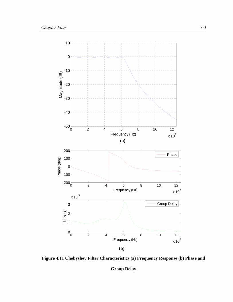
Chapter Four
60
0 2 4 6 8 10 12
x 105
-50
-40
-30
-20
-10
0
10
Frequency (Hz)
Mag
nitu
de (d
B)
(a)
0 2 4 6 8 10 12
x 105
-200
-100
0
100
200
Frequency (Hz)
Pha
se (d
eg)
0 2 4 6 8 10 12
x 105
0
1
2
3
x 10-6
Frequency (Hz)
Tim
e (s
)
Group Delay
Phase
(b)
Figure 4.11 Chebyshev Filter Characteristics (a) Frequency Response (b) Phase and
Group Delay

Chapter Four
61
The group delay, defined by Equation (4.1) , may be interpreted as the time that a
signal is delayed while passing through a filter.
ωωω
ddD )()( Θ
−= (4.1)
Group Delay is calculated by taking the derivative of the transmission phase with respect
to the frequency. Unfortunately, unequal Group Delay causes distortion in signal
composed of multiple frequencies; for example, unequal group delay will smear the
correlation peak creating uncertainty on where the peak really occurs. There is a trade-
off between the filter selectivity and the Group Delay. Figure 4.11b shows the Group
Delay present in the low pass filter. When calibrating a receiver, the Group Delay has to
be accounted for by adding this delay to the total receiver’s delay.
4.4 Digital Board
In digital systems, AGC is not used to maintain linearity in the RF and IF stages only but
in the analog-to-digital converter as well. As stated previously, most modern mobile
phones require a dynamic range between 80 to 100 dB, and the signal must be adjusted to
lie between the linear input ranges of the Analog-to-Digital Converter (ADC). This
means that the peak power is reduced by AGC in order to never exceed the full range of
the ADC. As seen in Figure 4.12, a VGA was inserted previous to the ADC to prevent
that the full range of the ADC is not exceeded.

Chapter Four
62
Figure 4.12 Digital Board Block Diagram
The 8-bit ADC output is connected directly to the FPGA board, a comparator is used to
evaluate if it is necessary to amplify or attenuate the signal using (4.2)
VOutputthenTQIIF
VOutputthenTQIIF
5
0
=<+
=≥+(4.2)
Since the output of the FPGA used to control the VGA is digital, an integrator is needed
to convert this output into an analog signal; the integrator will also add a time constant of
approximately 30 ms to its response.
The AD9059 analog-to-digital converter from Analog Devices was selected to be used in
the digital board. This converter is an 8-bit dual ADC which samples both analog inputs
at the same time. The specification of the AD9059; having an analog bandwidth of 120
MHz, maximum sampling rate of 60 MSPS and maximum jitter of 5 ps; exceeds the
requirements of this application.
FPGA
VGA
VGA ADC
ADC
Integrator
8
8
Sampling Clock
Gain Control

Chapter Four
63
It is important for the sampling clock to be virtually jitter free, since this instability
results in uncertainty as to when the analog input is actually sampled and will affect the
accuracy of the position location.
Figure 4.13 Timing Diagram for the AD9059
Figure 4.13 shows the timing diagram for the AD9059; as can be seen the ADC will
introduce a time delay. The total delay introduced by the ADC can be written as:
APDs
ttf
DelayTotal −+=3
where
sf is the sampling frequency
PDt is the propagation delay
At is the aperture delay
Figure 4.14 shows the developed digital board including the FPGA used.
N N+6
N+1
N+2
N+5
N+4
N+3
N+7
N-1 N-3 N-2 N N+1 N-4 N-3 N+4 N+3 N+2
Clock
Digital Output
Analog Input
tPD
tA
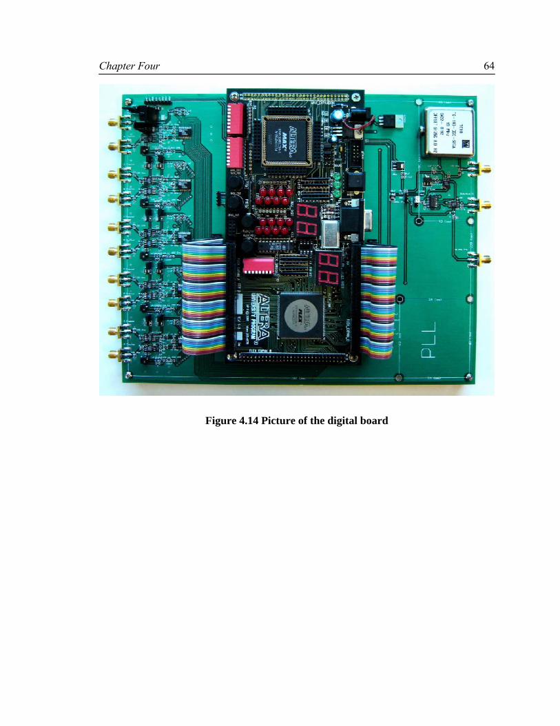
Chapter Four
64
Figure 4.14 Picture of the digital board

Chapter Five
65
CHAPTER FIVE: RECEIVER PARAMETERS
5.1 Receiver Performance
The receiver is often the most critical component of a wireless system, having the overall
purpose of reliably recovering the desired signal from a wide spectrum of transmitting
sources, interference and noise [Poza01]. This chapter introduces some fundamental
principles of a radio receiver design.
The fundamental tasks that the developed instrumentation receiver is required to perform
include:
• Selection of a desired signal from a potentially dense spectral environment while
rejecting adjacent channels, image frequencies, and interferences.
• High gain (~100 dB) to restore the low power of the received signal to a level
suitable for demodulation.
• Demodulation of the signal to recover the transmitted information.
The ability of the receiver to carry out this task can be measured using the following
parameters:
• Noise figure.
• Gain.
• Input Intercept Point.
• Dynamic Range.
• Sensitivity.
• Selectivity.

Chapter Five
66
A complete cascade analysis of these performance measures is carried out in this
chapter.
5.2 Noise Figure
The Noise Figure (NF) can be viewed as a measure in the degradation in the Signal-to-
Noise Ratio (SNR) between the input and the output of a component. The Signal-to-
Noise Ratio is the ratio of desired signal power to undesired noise power, and so is
dependent on the signal power. When noise and a desired signal are applied to the input
of a noiseless network, both noise and signal will be attenuated or amplified by the same
factor, so that the Signal-to-Noise Ratio will be unchanged. But if the network is noisy,
the output noise power will be increased more than the output signal power, so that the
output Signal-to Noise Ratio will be reduced. The noise figure, NF, is a measure of this
reduction in Signal-to-Noise Ratio [Poza05], and is defined as:
1≥=
o
o
i
i
NS
NS
NF (5.1)
where Si and Ni are the input signal and noise power, and So and No are the output signal
and noise powers. The input noise is defined as:
BkTNi 0= (5.2)
where
k is Boltzmann’s constant and
T0 is the temperature in Kelvin

Chapter Five
67
B is the bandwidth
At room temperature, the noise generated in a 1 Hz bandwidth is therefore
W10*4.043
(1Hz)J/K)(293K)10*(1.3821
23
−
−
=
=iN (5.3)
or -174 dBm/Hz when expressed as a power spectral density. From (5.2) it is easy to see
that the larger the bandwidth the greater the noise power. It is for this reason that the IF
filters need to be as narrow as possible in order to minimize the noise power just prior to
demodulation and detection.
This final IF filter will determine the overall noise bandwidth of the entire receiver since
it will be the most narrowband component in the entire chain prior to detection [Bess03].
A parameter of interest, important to all system, is the cascade noise figure. Equation
(5.4) is used to calculate this essential parameter.
1321321
4
21
3
1
21 ....
1.........111
−
−++
−+
−+
−+=
n
nT GGGG
NFGGG
NFGG
NFG
NFNFNF (5.4)
where
iNF is the noise figure of each component in the receiver
iG is the gain of each of each component in the receiver
Figure 5.1 shows the contribution to the noise figure made by each component in the
front-end receiver for different input power levels.
Note the contribution of the first two components, Low Noise Amplifiers (LNA) with
low noise figure is essential in order to obtain low cascade noise figure.
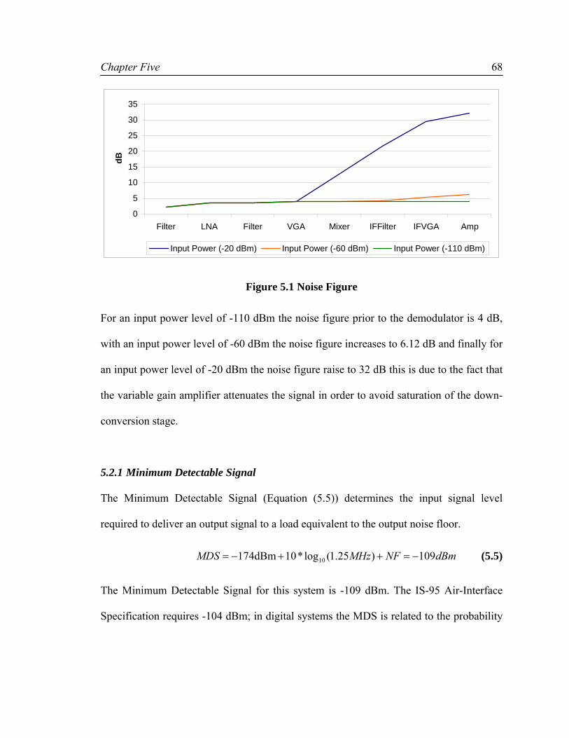
Chapter Five
68
0
5
10
15
20
25
30
35
Filter LNA Filter VGA Mixer IFFilter IFVGA Amp
dB
Input Power (-20 dBm) Input Power (-60 dBm) Input Power (-110 dBm)
Figure 5.1 Noise Figure
For an input power level of -110 dBm the noise figure prior to the demodulator is 4 dB,
with an input power level of -60 dBm the noise figure increases to 6.12 dB and finally for
an input power level of -20 dBm the noise figure raise to 32 dB this is due to the fact that
the variable gain amplifier attenuates the signal in order to avoid saturation of the down-
conversion stage.
5.2.1 Minimum Detectable Signal
The Minimum Detectable Signal (Equation (5.5)) determines the input signal level
required to deliver an output signal to a load equivalent to the output noise floor.
dBmNFMHzMDS 109)25.1(log*10dBm174 10 −=++−= (5.5)
The Minimum Detectable Signal for this system is -109 dBm. The IS-95 Air-Interface
Specification requires -104 dBm; in digital systems the MDS is related to the probability

Chapter Five
69
of a bit error equalling some threshold, and this sometimes requires some additional
margin.
5.3 Gain
The distribution of the gain in the receiver is a very important decision since it would
affect the Noise Figure and other important parameters in the receiver. For example, to
obtain the best NF adequate gain is required prior to the first mixer stage since mixers
tend to have poor NF.
-40
-20
0
20
40
60
80
100
Filter LNA Filter VGA Mixer IFFilter IFVGA Amp
Gai
n in
dB
Input Power (-20 dBm) Input Power (-60 dBm) Input Power (-110 dBm)
Figure 5.2 Overall System Gain
Figure 5.2 shows how the overall system gain is modified for different input signal
power. For example; as the desired signal increases in input power, the gain of the system
starts to decrease in order to minimize distortion. The gain in the IF stage is reduced first
to avoid increasing the noise figure and decrease sensitivity. When attenuation introduced
in the IF stage is not enough, attenuation in the RF stage is performed. This task is
performed by the Automatic Gain Control (AGC) circuitry.
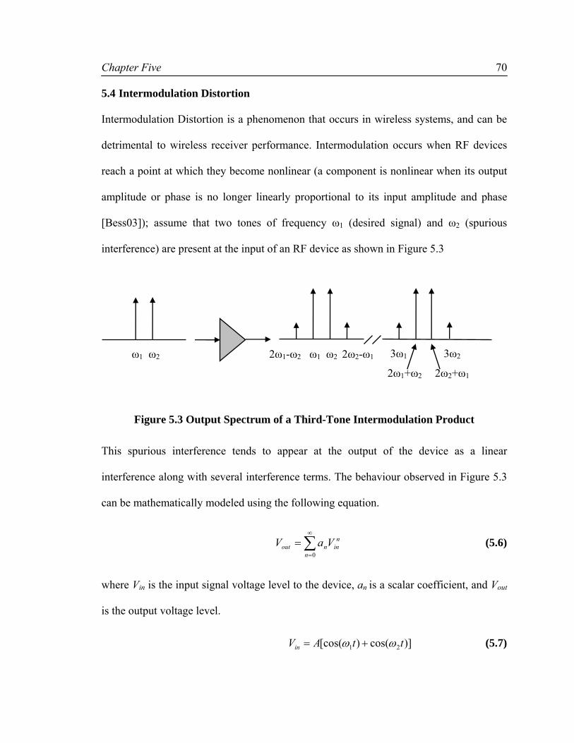
Chapter Five
70
5.4 Intermodulation Distortion
Intermodulation Distortion is a phenomenon that occurs in wireless systems, and can be
detrimental to wireless receiver performance. Intermodulation occurs when RF devices
reach a point at which they become nonlinear (a component is nonlinear when its output
amplitude or phase is no longer linearly proportional to its input amplitude and phase
[Bess03]); assume that two tones of frequency ω1 (desired signal) and ω2 (spurious
interference) are present at the input of an RF device as shown in Figure 5.3
Figure 5.3 Output Spectrum of a Third-Tone Intermodulation Product
This spurious interference tends to appear at the output of the device as a linear
interference along with several interference terms. The behaviour observed in Figure 5.3
can be mathematically modeled using the following equation.
nin
nnout VaV ∑
∞
=
=0
(5.6)
where Vin is the input signal voltage level to the device, an is a scalar coefficient, and Vout
is the output voltage level.
)]cos()[cos( 21 ttAVin ωω += (5.7)
ω1 ω2 2ω1-ω2 ω1 ω2 2ω2-ω1 3ω1 3ω2
2ω1+ω2 2ω2+ω1

Chapter Five
71
Equation (5.7) assumes that there is sufficiently large spectral separation between the
desired signal (ω1) and the interferer signal (ω2).
))]cos()(cos([ 2110 ttAaaVout ωω ++= (5.8)
In (5.8) the first two terms are linear terms; a0 being the DC term (negligible) and a1
being the device linear gain.
⎥⎥⎥
⎦
⎤
⎢⎢⎢
⎣
⎡
++−
++++=
)])cos(())[cos((
))2cos(1(2
))2cos(1(2
21212
2
2
1
2
2
ttA
tAtAaVout
ωωωω
ωω (5.9)
Equations (5.9) and (5.10) show that the output spectrum consists of harmonics of the
form 21 ωω nm + with 3,2,1,0, ±±±=nm . These combinations of the input frequencies are
called Intermodulation Products.
⎥⎥⎥⎥⎥⎥⎥⎥⎥⎥
⎦
⎤
⎢⎢⎢⎢⎢⎢⎢⎢⎢⎢
⎣
⎡
++−
+++−
++
++
=
)])2cos(())2[cos((4
3
)])2cos(())2[cos((4
3
)3cos(4
)3cos(4
)cos(2
3)cos(2
3
2121
3
2121
3
2
3
1
3
2
3
1
3
3
ttA
ttA
tAtA
tAtA
aVout
ωωωω
ωωωω
ωω
ωω
(5.10)
The cubed term, equation (5.10), leads to six Intermodulation Products: ,3,3 21 ωω
12211221 22,2,2 ωωωωωωωω −−++ and . The first four of these will be located far from
ω1 and ω2, and will be outside the passband of the component.
Nevertheless the two difference terms produce products located near the original input
signals at ω1 and ω2 therefore they cannot be easily filtered from the passband of an

Chapter Five
72
amplifier. Figure 5.3 shows a typical spectrum of the third-order two-tone
intermodulation products.
For an arbitrary input signal consisting of many frequencies of varying amplitude and
phase, the resulting in-band intermodulation products will cause distortion of the output
signal. This effect is called third-order intermodulation distortion [Poza01].
5.5 Third-Order Intercept Point
The concept of Intercept Point (IP) enables the distortion properties of several cascaded
devices to be calculated. It can be approximately calculated as fallows:
121211 3...1......
31
31
31
31
IPGGGIPGGIPGIPIP NNNNNNNNT −−−−
++++= (5.11)
The intercept point, measured in dBm, is a figure of merit for intermodulation product
suppression; a high intercept point indicates a high suppression of undesired
intermodulation products.
-80-60-40-20
020406080
100120
Filter LNA Filter VGA Mixer IFFilter IFVGA Amp
dB
Input Power (-20 dBm) Input Power (-60 dBm) Input Power (-110 dBm)
Figure 5.4 Input Intercept Point

Chapter Five
73
The third-order intercept point is the theoretical point where the desired signal and the
third order distortion have equal magnitude.
Figure 5.4 shows the third input intercept point for different input power levels; it can be
seen that for an input power level of -110 dBm the input intercept point is greatly
reduced. However, linearity is most important in the wideband section of the radio
receiver where multiple channels are present and the possibility of intermodulation arises.
Following the IF filter, interfering channels have been reduced in power, and the strict
requirements on intercept point can be relaxed [Bess03].
Nonlinearity in a system or subcircuit creates AM to PM conversion that plays a major
role in phase noise performance. When the input signal level changes, a well behaved
amplifier maintains the same delay time to for a signal to travel through the circuit. AM-
to-PM conversion is a measure of how the phase nonlinearity varies with signal
magnitude.
AM-to-PM conversion is critical in systems based on phase modulation, such as
Quadrature Phase Shift Keying (QPSK), since phase distortion can cause signal
degradation in analog systems and increase bit-error rate (BER) in digital systems.
AM-to-PM conversion is usually defined as the change in output phase for a 1-dB
increment in the input power to an amplifier, expressed in degrees/dB.
5.6 Receiver Dynamic Range
A measure of the receiver’s immunity to the problem of Intermodulation Distortion is the
receiver Dynamic Range; which is discussed in this section. Dynamic Range of an
amplifier or receiver is the range of signal power levels over which a system will operate

Chapter Five
74
properly. It should be emphasized that a receiver’s dynamic range and AGC range are
usually two different quantities.
The low power limit is generally set by noise; this limit was described as the Minimum
Detectable Signal in the preceding paragraphs. The upper limit is generally set by third-
order intercept point [Egan03]. In a high Dynamic Range receiver, expect all stages to
contribute to the noise figure, because strong signals will require insertion loss distributed
throughout.
Figure 5.5 Intercept Diagram
When testing a receiver (or amplifier) for the upper dynamic range limit, it is common to
apply a single test frequency and determine the 1-dB compression point. 1-dB
compression point occurs when the subtraction of the output power versus the input
power is one dB lower than the expected power. The 1-dB compression point of an
x
3x
Spourious Free Dynamic Range O
utpu
t Pow
er (d
Bm
)
Input Power (dBm)
Noise Floor
IP3
1dBCP
Intercept Point
1 dB
Compression Point

Chapter Five
75
amplifier is commonly measured at the output but it can be easily transferred to the
input just by subtracting the gain of the amplifier.
Since the intercept point is a fictitious point, an extrapolation of the fundamental
components in a linear fashion needs to be done. From the intercept diagram in Figure
5.5 it can be demonstrated that
dBdBIP CP 6.1013 += (5.12)
A more useful measure is the Spurious Free Dynamic Range, SFDR, and it is defined as
the range of input power level from which the output signal just exceeds the output noise
floor, and for which the distortion components remain buried below the noise floor.
Using geometric equations based on Figure 5.5; (5.13) can be obtained,
FloorNoiseIPx −= 33 (5.13)
Since the Spurious Free Dynamic Range is SFDR=2x, (5.14) can be easily obtained.
( )
( )( )NFGBIPSFDR
FloorNoiseIPSFDR
−−−+=
−=
log*101743232
3
3
(5.14)
The Spurious Free Dynamic Range (at the output of the IF filter) obtained for the
designed receiver was:
( ) ( )( ) dBmFloorNoiseIPSFDR 8.489.856.1232
32
3 =−−−=−= (5.15)
However, this calculation ignores the impact of the automatic gain control; for example,
the IP3 value used in (5.15) corresponds to the IP3 value for small input power level; in
Chapter Five
76
presence of strong signals the gain is reduced (see Figure 5.2) and the IP3 increases;
thus the SFDR increases.
5.7 Receiver Selectivity
Another important characteristic of a receiver is its selectivity; which is defined as the
ability of a receiver to adequately extract the desired signal in presence of strong adjacent
frequency interferers and channel blockers. The selective filter must be sufficiently sharp
to suppress the interference from adjacent channel and spurious responses. However, the
filter has to be broad enough to pass the highest sideband frequencies with acceptable
distortion in amplitude and phase. For the designed receiver the IF filter sets the
selectivity of the receiver.
5.8 Receiver Sensitivity
Sensitivity is a measure of the receiver’s ability to detect a signal of a given level, in
other words, sensitivity is the absolute power level that gives the required Signal-to-
Noise Ratio. Mathematically, sensitivity is defined as the sum of the Minimum
Detectable Signal and the required output Signal-to-Noise Ratio given by (5.16)
SNRMDSS dBmdBm += (5.16)
where
MDS is the Minimum Detectable Signal
SNR is the Signal-to-Noise Ratio for a specific quality of received information

Chapter Five
77
This equation indicates that sensitivity improves (becomes more negative) with
decreasing noise figure. Since MDS is a function of the bandwidth, sensitivity is heavily
influenced by the IF bandwidth.
5.9 Effect of Automatic Gain Control
Automatic Gain Control (AGC) is used for many reasons. First, detection circuits usually
have a range of input power levels over which they operate properly. As introduced
before; if the input signal power is too strong it causes overload or distortion. If the input
signal power is too small, noise overcomes the detection circuits.
Second, in mobile receivers the signal power may experience extreme excursions. A
properly designed AGC system will compensate for these extreme excursions [Blank98].
Third, adjusting the gain extends the dynamic range of the receiver. However, the impact
of using of an AGC over the dynamic range is not always obvious and will require some
analysis.
Therefore, it is necessary to consider the gain, the noise figure and the input intercept
point altogether since these are the principal trade-offs in setting an AGC level.
For instance, consider a Variable Gain Amplifier (VGA) that can either amplify or
attenuate the signal after the LNA. If the input signal power is too large then the VGA is
used as an attenuator, this will prevent overload of following stages but it will increase
the Noise Figure (see Figure 5.1 for an input signal power of -20 dBm).
If the input signal power is too small the VGA is used as an amplifier, in this case the
Noise Figure is minimized but the third-order intercept point is reduced (see Figure 5.4
for an input signal power of -110 dBm).

Chapter Six
78
CHAPTER SIX: TIME SYNCHRONIZATION AND LOCAL OSCILLATORS
6.1 Base Stations Time Synchronization
CDMA systems locks the BS system time and clocks to the Global Positioning System
(GPS). The Pulse Per Second (pps) signal generated by the GPS is used to control the
start of the Pilot code generator at each BS and to phase lock the Pilot code generator to
other code generators in the system.
6.2 Receiver Synchronization
In order to achieve time synchronization with the BS, the phase of the 10 MHz
Temperature Controlled Crystal Oscillator (TCXO) is continuously measured relative to
the GPS 10 MHz clock. The block diagram of the time synchronization scheme is shown
in Figure 6.1.
Figure 6.1 Timing Synchronization
LO Synthesizers
Relative Phase Measurement
GPS Reference Receiver 10 MHZ 1pps
TCXO Source
Data Storage Memory
External PC
ADC External Rubidium Source
CDMA RX
Data Multiplexing
Chapter Six
79
The receiver can be driven by either an internal TCXO oscillator (Table 6-1 shows the
characteristics of the TCXO) or an external Rubidium Oscillator. Both of these oscillators
are free-running. To synchronize the oscillator to the GPS clock, a phase measurement
circuit is used as shown in Figure 6.1. The phase is used to rotate the CDMA sampled
data and align it to the equivalent sampling of the 10 MHz GPS clock been used.
When the GPS signal is known to be poor as indicated by the GPS status output, the
relative phase measurements are invalid since the receiver data cannot be accurately
rotated. However, the Rubidium or TCXO clocks are sufficiently stable over the short-
term of the measurement to ensure sufficient phase coherency [Lope05].
Another key parameter of this oscillator is its phase noise, since phase noise generated at
the TCXO oscillator is multiplied by the ratio of the RF frequency to its frequency
through the synthesis process.
The detailed order of events for the sampling are listed below:
• The leading edge of the 1 pulse per second (pps) signal from the GPS receiver is
received by the FPGA.
• The first sample is taken coincidently with the rising edge of the 10 MHz TCXO
clock. That is, the 1 pps signal enables the sampling to start but the actual
sampling is synchronized to the TCXO. The time between the leading edge of 1
pps and the time the first sample is taken is variable by a range of one clock cycle
of the TCXO which is 100 ns.
• The First Sample pulse is sent to the GPS receiver. The GPS receiver determines
the absolute time of the rising edge of the First Sample pulse. This becomes the
First Sample Time.
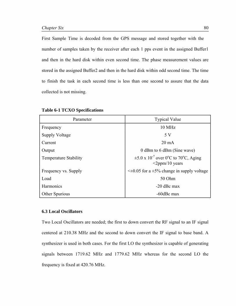
Chapter Six
80
First Sample Time is decoded from the GPS message and stored together with the
number of samples taken by the receiver after each 1 pps event in the assigned Buffer1
and then in the hard disk within even second time. The phase measurement values are
stored in the assigned Buffer2 and then in the hard disk within odd second time. The time
to finish the task in each second time is less than one second to assure that the data
collected is not missing.
Table 6-1 TCXO Specifications
Parameter Typical Value
Frequency 10 MHz
Supply Voltage 5 V
Current 20 mA
Output 0 dBm to 6 dBm (Sine wave)
Temperature Stability ±5.0 x 10⁻⁷ over 0oC to 70oC, Aging <2ppm/10 years
Frequency vs. Supply <±0.05 for a ±5% change in supply voltage
Load 50 Ohm
Harmonics -20 dBc max
Other Spurious -60dBc max
6.3 Local Oscillators
Two Local Oscillators are needed; the first to down convert the RF signal to an IF signal
centered at 210.38 MHz and the second to down convert the IF signal to base band. A
synthesizer is used in both cases. For the first LO the synthesizer is capable of generating
signals between 1719.62 MHz and 1779.62 MHz whereas for the second LO the
frequency is fixed at 420.76 MHz.

Chapter Six
81
6.3.1 Frequency offset
Oscillator instability and Doppler shift (only in the kinematic condition) create
differences between the local oscillator used to downconvert the received CDMA signal
and the received signal itself; this is frequency offset it is not compensated in the CDMA
receiver, as a consequence this will result in an imperfect downconversion.
However, careful calibration of the TCXO can greatly reduce the frequency offset; a two-
dimensional search is performed to eliminate the frequency offset and acquire the CDMA
pilot signal. Further discussion about frequency offset removal is carried out in chapter 8.
Figure 6.2 shows a plot of SNR vs. Frequency Offset
-100 -50 0 50 1000
50
100
150
200
250
300
Frequency Offset (Hz)
SN
R
Figure 6.2 SNR vs. Frequency Offset (averaged)

Chapter Six
82
The previous plot was generated by computing the Signal-to-Noise Ratio of one of the
strongest BS by adding different frequency offsets (from -100 Hz to 100 Hz), this
procedure was averaged in 5 trials.
The previous plot shows as well how critical is the selection of the correct frequency step
size when a two-dimensional search is performed; since large frequency step size can
seriously affect the acquisition of the MS.
6.4 Phase Noise and Spurious Outputs
In radio receivers, phase noise and spurious output of local oscillators can often be
critical to receiver performance. Phase noise and spurious output can be a limiting factor
in receiver dynamic range, as well as a contributor to poor signal to noise ratios and bit
error rates of demodulated signals. In addition, spurious outputs can result in spurious
signals being received which are not actually present in the environment [Kuhn95].
6.4.1 Phase Noise
Phase Noise refers to the short-term random fluctuation in the frequency (or phase) of an
oscillator signal. Noise produced by local oscillators or frequency synthesizers is
critically important in practice because it may severely affect the performance of the
receiver. Besides adding to the noise level of the receiver, a noisy local oscillator will
lead to downconversion of undesired nearby signals, thus limiting the selectivity of the
receiver and how closely adjacent channels may be spaced [Poza01].
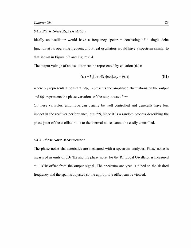
Chapter Six
83
6.4.2 Phase Noise Representation
Ideally an oscillator would have a frequency spectrum consisting of a single delta
function at its operating frequency; but real oscillators would have a spectrum similar to
that shown in Figure 6.3 and Figure 6.4.
The output voltage of an oscillator can be represented by equation (6.1):
)](cos[)](1[)( 00 tttAVtV θω ++= (6.1)
where V0 represents a constant, A(t) represents the amplitude fluctuations of the output
and θ(t) represents the phase variations of the output waveform.
Of these variables, amplitude can usually be well controlled and generally have less
impact in the receiver performance, but θ(t), since it is a random process describing the
phase jitter of the oscillator due to the thermal noise, cannot be easily controlled.
6.4.3 Phase Noise Measurement
The phase noise characteristics are measured with a spectrum analyzer. Phase noise is
measured in units of dBc/Hz and the phase noise for the RF Local Oscillator is measured
at 1 kHz offset from the output signal. The spectrum analyzer is tuned to the desired
frequency and the span is adjusted so the appropriate offset can be viewed.

Chapter Six
84
Figure 6.3 Output Spectrum of the RF LO
The difference between the carrier and the noise level minus 10*log10(Resolution
Bandwidth) is equal to the phase noise in dBc/Hz. A 40 Hz resolution bandwidth was
used for the RF and IF local oscillator phase noise evaluation. The phase noise for this
signal is:
OffsetkHzHzdBcdBmdBm 1@/02.71)40(log*10)65(10 10 −=−−+
Note in Figure 6.3 that the output power of the RF LO is around -11 dBm. However a
level 7 mixer must be driven by this signal. In order to solve this problem an amplifier at
the RF local oscillator was added. In Figure 6.4 the synthesizer output signal for IF local
oscillator could be readily noticed.

Chapter Six
85
Figure 6.4 Output Spectrum of the IF LO
The phase noise for this signal is:
OffsetkHzHzdBcdBmdBm 1@/02.66)40(log*10)50(0 10 −=−−+
The phase noise values are within the IS-95A standard specifications.
6.5 Allan Variance
The Allan variance is a measurement of stability in clocks and oscillators. It is also
known as the two-sample variance. It is defined as one half of the time average of the
squares of the differences between successive readings of the frequency deviation
sampled over the sampling period. The Allan variance depends on the time period used
between samples: therefore it is a function of the sample period, as well as the
distribution being measured, and is displayed as a graph rather than a single number. A
low Allan variance is a characteristic of a clock with good stability over the measured
period. For the clocks the Allan variance is given by:

Chapter Six
86
∑−
=+ −
−=
1
1
21
2 )()1(2
1)(n
kkky yy
nτσ (6.2)
where
ky is the clock at time tk
kk yy −+1 is the change in clock error over time interval kk tt −+1
τ is the averaging time interval kk tt −+1
n is the number of samples
Allan variance was used as a measure of frequency stability of the TCXO used as
referencence oscillator of the developed receiver. More information about this
measurements can be found in [Lu05]

Chapter Seven
87
CHAPTER SEVEN: RECEIVER TEST
7.1 Receiver Test
Receiver tests aim to quantify the performance of the developed CDMA receiver in
normal operation conditions and in presence of an interferer. Tests for this particular
receiver consist of measuring the single tone interference, Signal-to-Noise Ratio vs.
Integration time and the phase difference stability.
7.2 Single-Tone Desensitization
The desensitization of the receiver determines its ability to successfully operate under
strong interferers [Kim05]. They are specified separately from in-band and out-of-band
conditions. In the cellular band and in the PCS band, the single tone desensitization is a
measure of the receiver’s ability to receive a CDMA signal at its assigned channel in
presence of a single tone with -30 dBm power and spaced at a given 900 kHz frequency
offset from the PCS band desired signal frequency center. Figure 7.1 shows the settings
for this specific test. The input signal to the receiver front-end consist of the desired
signal provided by the antenna (placed on the roof of the CCIT building) connected to a
power combiner; plus jammers which may be transmitted from other systems.
In this test, a signal generator was used to generate the interferer signal with the
appropriate frequency offset from the desired CDMA signal, this signal was fed into the
power combiner as well.

Chapter Seven
88
Figure 7.1 Test settings
The presence of a single tone jammer can degrade the receiver performance by two
different mechanisms. First, the jammer can affect the signal power level measured by
the RF power detector and this will increase the attenuation introduced by the variable
gain amplifier; hence, it will increase the noise figure and decrease the SNR.
Second, the weak desired signal can be desensitized if the jammer is strong enough to
push the front end to compression [Chen97].
Figure 7.2 shows the correlation peaks without the interferer signal; the measured SNR
was 21.6 dB.
Receiver
Power Combiner
Signal Generator

Chapter Seven
89
0 0.005 0.01 0.015 0.02 0.0250
2000
4000
6000
8000
10000
12000
14000
16000
18000
Time (s)
Cor
rela
tion
Pow
er
Figure 7.2 Correlation Peaks with no interference signal
0 0.005 0.01 0.015 0.02 0.0250
2000
4000
6000
8000
10000
12000
14000
16000
18000
Time (s)
Cor
rela
tion
Pow
er
Figure 7.3 Correlation Peaks with interference signal

Chapter Seven
90
Figure 7.3 shows the correlation peaks with the interferer signal; as it can be seen the
SNR has been reduced to 18.8 dB. This reduction in the SNR (less than 3 dB) is not
significant and does not represent a threat to the signal acquisition since the four major
acquired base station still have a large SNR.
7.3 SNR vs. Integration Time
As expected, with each increment of the integration time the SNR increases. The problem
of having a large integration time is that more stable oscillators are needed; otherwise the
correlation peak starts to “smear”. Therefore, there is a trade off between the SNR and
the Integration Time where the Integration Time should be kept as small as possible, but
maintaining a good SNR. Figure 7.4 shows a plot of SNR vs. Integration Time.
0 0.1 0.2 0.3 0.4 0.5 0.6 0.7 0.810
0
101
102
103
Integration Time (s)
SN
R
Figure 7.4 SNR Vs Integration time

Chapter Seven
91
Real data was used to plot the previous figure, averaged over three trials.
7.4 Phase Difference Stability
The phase stability is a major concern when defining the direction of arrival. In order to
measure the phase stability of the developed receiver a total of 50 measurements where
collected with 60 seconds intervals between them. Only one antenna was used in this test,
the signal was split away in order to feed the five channels.
0 10 20 30 40 50100
150
200
250
300
350
400
450
500
Samples
Pha
se D
iffer
ence
(in
degr
ees)
Ch1-Ch2Ch1-Ch3Ch1-Ch4Ch1-Ch5
Figure 7.5 Phase Difference
As Figure 7.5 illustrates, there is no major fluctuation in phase for any of the receiver’s
channels which indicates that the receiver is stable and can be used to collect AOA
measurements. Figure 7.5 was generated using the phase of the strongest correlation
peak.
Chapter Eight
92
CHAPTER EIGHT: RANGE AND ANGLE MEASUREMENT ANALISYS
8.1 Introduction
The previous chapters dealt with the hardware receiver design and time synchronization
of the receiver with GPS time. From the design perspective, the receiver now requires
good post-mission processing algorithms to process the received CDMA pilot data and to
obtain the position estimate. In addition, various characteristics of the receiver will be
investigated using the post-mission signal processing.
8.2 Post-mission processing
Post-mission processing involves the processing of the received CDMA pilot data stored
in the computer’s memory for further analysis. The first step is to read the data from the
computer memory and convert it to appropriate data formats for processing.
The file contains both the in-phase and the quadrature phase components of the pilot
signal then; the data is processed to obtain the in-phase and the quadrature phase
components separately.
The data stored in the computer memory is obtained by sampling the 1.25 MHz signal at
2 MHz rate. Thus, each pilot PN chip corresponds to approximately 0.61 samples. As a
result, data re-sampling must be performed to facilitate subsequent signal processing.
This can be achieved in two ways:
• The received data samples could be re-sampled at a higher rate to match an
integral multiple of the chip rate. For example, the 2 MHz samples could be
sampled at a rate of N*1.2288 MHz (N=2, 3…).

Chapter Eight
93
• The locally generated signal could be re-sampled to match the 2 MHz sampling
rate of the received data samples.
While the aforementioned techniques are slightly different, the end result is the same.
8.2.1 Two-Dimensional Acquisition
The received CDMA pilot signal acquisition process consists of a two-dimensional
search in both frequency (due to residual frequency offset) and time. The received
baseband signal has some residual frequency offset that needs to be corrected during the
acquisition process.
The frequency search bin is inversely related to the coherent integration time. To
decrease the search size as well as to reduce the execution time, the frequency is searched
in an adaptive fashion. At first, a reasonable integration time is used to find the
correlation peak. In most cases, a frequency resolution of 0.01 Hz is achieved with this
method with reasonable complexity.
8.3 CDMA Acquisition
The problem of CDMA acquisition encompasses BS frequency identification (or
equivalently the channel number) and the PN offset. As discussed in Chapter 3, the
physical IS-95A CDMA channels are allocated in discrete frequency bands (5 or 15
MHz) in the PCS band. Hence, the first step towards channel identification is to find
these frequency bands in the PCS spectrum.

Chapter Eight
94
8.3.1 Base Station Identification
The brute force approach of CDMA channel identification involves searching of all
physical channels in the 1930 to 1990 MHz band. Since the physical CDMA channels are
separated by 50 KHz, this corresponds to a search of 1200 frequency channels. The
physical CDMA channels occur in discrete frequency bands of 5 or 15 MHz.
The search can be greatly reduced by searching for these discrete bands and then
searching all the frequency bins in these bands. In the initial test setup, the output of the
140o directional antenna was fed into the spectrum analyzer and the PCS band was
scanned for the discrete frequency bands. The measured frequency spectrum is shown in
Figure 8.1; three frequency bands in the range 1945 – 1949 MHz, 1955 – 1959 MHz and
1979 – 1983 MHz were identified as potential CDMA bands.
Figure 8.1 Frequency Spectrum Showing Probable CDMA Channels

Chapter Eight
95
The probable frequency bands are encircled in the plot. Thus, the search size could be
reduced from 1200 frequency channels down to 100 frequency channels. However, a
search of 100 frequency bins with 32768 chips offsets for each frequency bin is still
considerable.
In addition, the received baseband CDMA signal will still contain a residual frequency
offset. This frequency offset depends on the stability of the oscillator, mobile station
velocity, and the frequency synthesizer in the CDMA receiver. However, the cyclo-
stationary property of the pilot sequence could be utilized to minimize the search. Let the
sampled complex baseband signal be expressed as,
)()]()([)( 2 knkjckceky qiFkj
k ++= Δ− πα (8.1)
where
ci(k) and cq(k) are the in-phase and the quadra-phase pilot sequences
αk is the phase attenuation
ΔF is the residual frequency offset
n(k) is the AWGN noise
Since, the pilot sequence repeats every 26.67 ms and assuming the variation of
propagation characteristics to be small,
)()( Kkyky −= (8.2)
)()( Kknkn −≠ (8.3)
Kkk −≈ αα (8.4)
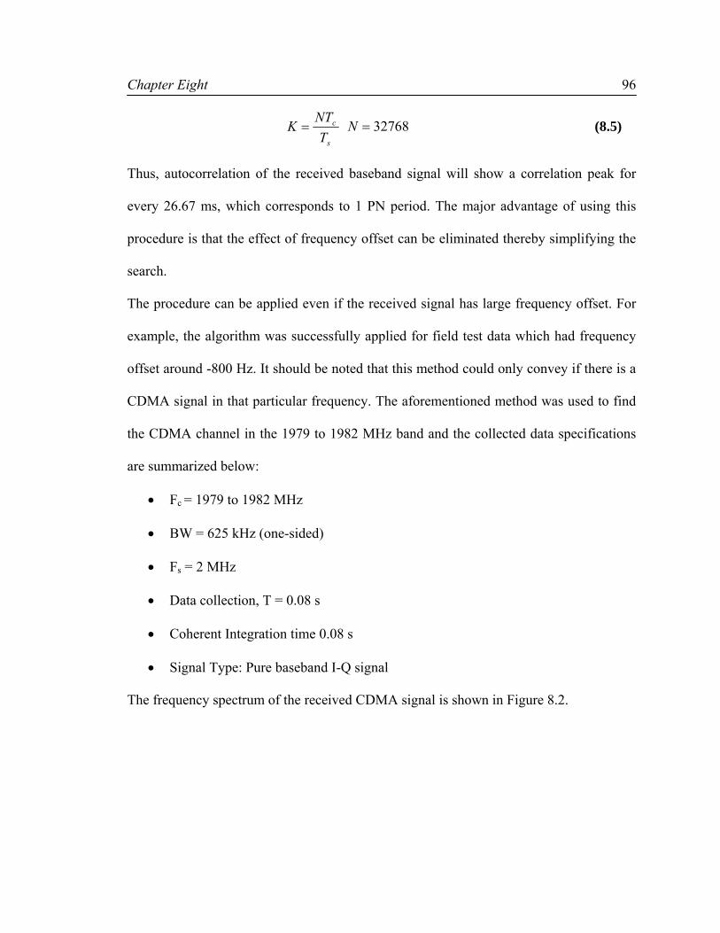
Chapter Eight
96
s
c
TNTK = 32768=N (8.5)
Thus, autocorrelation of the received baseband signal will show a correlation peak for
every 26.67 ms, which corresponds to 1 PN period. The major advantage of using this
procedure is that the effect of frequency offset can be eliminated thereby simplifying the
search.
The procedure can be applied even if the received signal has large frequency offset. For
example, the algorithm was successfully applied for field test data which had frequency
offset around -800 Hz. It should be noted that this method could only convey if there is a
CDMA signal in that particular frequency. The aforementioned method was used to find
the CDMA channel in the 1979 to 1982 MHz band and the collected data specifications
are summarized below:
• Fc = 1979 to 1982 MHz
• BW = 625 kHz (one-sided)
• Fs = 2 MHz
• Data collection, T = 0.08 s
• Coherent Integration time 0.08 s
• Signal Type: Pure baseband I-Q signal
The frequency spectrum of the received CDMA signal is shown in Figure 8.2.
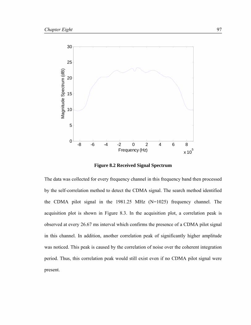
Chapter Eight
97
-8 -6 -4 -2 0 2 4 6 8
x 105
0
5
10
15
20
25
30
Frequency (Hz)
Mag
nitu
de S
pect
rum
(dB
)
Figure 8.2 Received Signal Spectrum
The data was collected for every frequency channel in this frequency band then processed
by the self-correlation method to detect the CDMA signal. The search method identified
the CDMA pilot signal in the 1981.25 MHz (N=1025) frequency channel. The
acquisition plot is shown in Figure 8.3. In the acquisition plot, a correlation peak is
observed at every 26.67 ms interval which confirms the presence of a CDMA pilot signal
in this channel. In addition, another correlation peak of significantly higher amplitude
was noticed. This peak is caused by the correlation of noise over the coherent integration
period. Thus, this correlation peak would still exist even if no CDMA pilot signal were
present.

Chapter Eight
98
0 0.01 0.02 0.03 0.04 0.05 0.06 0.07 0.080
2000
4000
6000
8000
10000
12000
14000
16000
18000
Time(s)
Cor
rela
tion
Pow
er
53.3 ms26.67 ms
1st Period 2nd Period 3rd Period
Figure 8.3 Self-correlation Acquisition to Detect the Presence of CDMA Signal
The same procedure was repeated for the other frequency bands to detect the presence of
CDMA pilot signal. Again, the presence of CDMA signal was detected in the 1947.5
MHz frequency which corresponds to channel 350.
8.3.2 CDMA Base Station Identification
The self correlation method explained in the previous section does not provide any other
information other than the presence of a CDMA signal. However, since the carrier
frequency was already identified the search space is significantly reduced. The next step
in the CDMA pilot acquisition involves the 2-D acquisition of residual frequency offset
Δf, and the corresponding time offset of the BS. The received baseband signal is

Chapter Eight
99
coherently integrated with the locally generated pilot PN sequence to obtain these
parameters. The frequency step size was chosen according to (8.6),
pitTf
32
≤Δ (8.6)
where
fΔ is the frequency step size
Tpit is the pre-detection integration time.
The pre-detection integration time was fixed at Tpit = 0.08 s with the corresponding
frequency step size of 5 Hz. The carrier frequency was set to 1981.25 MHz. the
frequency search was limited to ±150 Hz. This is mainly due to the fact that both the BS
and the receiver are stationary. However, in the case of kinematic measurements and low
outdoor temperatures, the search must be increased. The estimated frequency offset was
found to be -27 Hz which becomes crucial for long coherent integration time over several
hundred milliseconds. The correlation plot for the collected data at 1981.25 MHz is
shown in Figure 8.4.

Chapter Eight
100
0 0.01 0.02 0.03 0.04 0.05 0.06 0.07 0.080
0.5
1
1.5
2
2.5
3
3.5
4x 10
4
Time (s)
Cor
rela
tion
Pow
er
Figure 8.4 CDMA Correlation as a Function of Code Offset
In the above correlation plot, a minimum of 3 BS can be observed. The correlation peaks
occur every 26.67 ms corresponding to the pilot PN sequence period. During this data
collection, the receiver was connected to the roof top antenna through a cable with length
greater than 30 m.
Now that the correlation peaks corresponding to different BS are identified, their relative
time offsets and the actual BS identification needs to be determined. The relationship
between the pilot offset and GPS time is illustrated in Figure 8.5.

Chapter Eight
101
Figure 8.5 CDMA Pilot Offsets Relative to GPS PPS Time Mark
From the correlation peaks, it is easy to find the relative time offset between the base
stations. Since, the base station PN offsets are multiples of 64 chips (52.08 µs) the
propagation delay from the base stations can be directly determined by removing this PN
offset. Once the relative time or time differences of arrivals are known, trilateration is
used to find the MS position.
For example, a 64 chips BS offset would result in a 52.083 μs time offset which is 15.625
km. In order for this to introduce ambiguity, the MS has to receive pilot signals from a
BS which is at least 15.625 km distant. In reality, it is nearly impossible to receive signals
from a BS at a distance of 15.625 km due to power control, free space attenuation, fading
and shadowing effects. In addition, the BS offsets are chosen so that this separation is
large.
Base station 1 start of pilot code
GPS Even Second Time Mark
Base station 0 start of pilot code Base station 511 start of pilot code
64 chips
26.6 ms

Chapter Eight
102
8.4 Effect of Antenna Pattern
The effect of the antenna pattern readily affects the number of Base Stations acquired, the
system performance and the multipath. For example, CDMA receivers are usually
equipped with omni-directional antennas to facilitate RAKE combining of multipath
components. However, multipath propagation adversely affects the position estimation
performance of the receiver. In order to evaluate the antenna pattern on the system
performance, two different antennas, namely directional and omni-directional, were used.
The data was collected first for the omni-directional antenna and then this antenna was
replaced by the directional antenna, both antennas shared the same cable; this precaution
was taken in order to avoid differences in cable length and loss which can severely affect
the received data. The directional antenna was oriented towards Downtown.
(a) (b)
Figure 8.6 (a) Directional Antenna (b) Omni-Directional Antenna
The antenna gains for the directional and omni-directional antennas were 7 dBi and 5.4
dBi respectively. The received pilot signals were coherently integrated over 0.08 s for
both cases. The received number of Base Stations was slightly higher for the omni-
directional antenna, as expected; this is because the omni-directional antenna has a

Chapter Eight
103
constant gain in the azimuth and will be able to receive signals from all directions,
which is not the case for the directional antenna.
For the strongest base station the correlation power was higher for the data acquired with
the omni-directional antenna despite the fact that this antenna has less gain than the
directional antenna. Since information of BS location was not available during the time of
data collection, it is possible that the strongest Base Station was out of the 1400
Horizontal Beamwidth of the directional antenna.
The correlation peaks corresponding to the strongest, second strongest and BS with
multipath components are shown in Figure 8.7.
8.958 8.96 8.962 8.964 8.966 8.968 8.97 8.972 8.974
x 10-3
0
0.5
1
1.5
2
2.5
3
x 104
Time (s)
Cor
rela
tion
Pow
er
DirecOmni
(a)
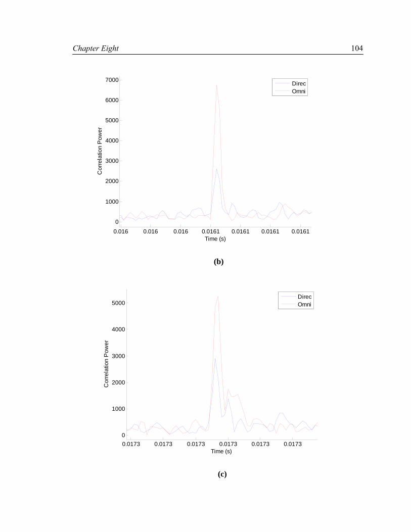
Chapter Eight
104
0.016 0.016 0.016 0.0161 0.0161 0.0161 0.01610
1000
2000
3000
4000
5000
6000
7000
Time (s)
Cor
rela
tion
Pow
er
DirecOmni
(b)
0.0173 0.0173 0.0173 0.0173 0.0173 0.01730
1000
2000
3000
4000
5000
Time (s)
Cor
rela
tion
Pow
er
DirecOmni
(c)

Chapter Eight
105
0.0275 0.0275 0.0275 0.0275 0.0275 0.0275 0.0275 0.02750
1000
2000
3000
4000
5000
6000
7000
8000
9000
10000
Time (s)
Cor
rela
tion
Pow
er
DirecOmni
(d)
Figure 8.7 Correlation Plots for Different BSs. (a) Strongest BS (b) Second Strongest
(c) With Multipath Components (d) Directional antenna with higher gain
From Figure 8.7 (c), it may be observed that the omni-directional antenna resulted in one
LOS component and two multipath components of approximately equal strength which
indicates of NLOS propagation. In addition, the directional antenna shows a multipath
component as well.

Chapter Eight
106
8.5 Effect of Predetection Integration Time
Predetection Integration is the signal processing after the baseband signal has been
converted to digital by the A/D converter. The coherence integration time is actually a
statistical measure of the time duration over which the impulse response is essentially
invariant [Rapp02].
In previous sections, the effect of coherent integration time on sensitivity and
detectability was discussed. The output SNR, accuracy and stability also depend on the
coherent integration time.
8.955 8.96 8.965 8.97 8.975
x 10-3
0
1
2
3
4
5
6
x 104
Time (s)
Cor
rela
tion
Pow
er
0.08s Int. Time0.16s Int. Time
Figure 8.8 Correlation Peak of the Strongest Base Station for Different Coherent
Integration Time
For the developed system, accuracy and stability critically depend on the coherent
integration time. To evaluate the effect of coherent integration on the correlation peak,

Chapter Eight
107
the received data was processed with two different integration times namely 0.08 s
and 0.16 s. The correlation peak corresponding to the strongest BS for different
integration times is shown in Figure 8.8. From the correlation plot, it is observed that the
higher correlation gain is achieved with 0.16 s coherent integration.
However, the spread in the correlation for 0.16 s coherent integration is wider than that of
the 0.08 s integration. This spread is mainly caused by oscillator frequency drift and time
varying multipath propagation.
5.5 6 6.5 7 7.5 8 8.5 9 9.5 10
x 10-6
0
2000
4000
6000
8000
10000
12000
14000
Time (s)
Cor
rela
tion
Pow
er
Epoch 1Epoch 2Epoch 3Epoch 4Epoch 5
(a)

Chapter Eight
108
5.5 6 6.5 7 7.5 8 8.5 9 9.5 10
x 10-6
0
0.5
1
1.5
2
x 104
Time (s)
Cor
rela
tion
Pow
er
Epoch 1Epoch 2Epoch 3Epoch 4Epoch 5
(b)
Figure 8.9 Correlation Peak of Strongest BS at Different Time Epochs (a) 0.08 s
Integration Time (b) 0.16 s Integration Time
The stability of the correlation estimates directly affects the accuracy and stability of the
resulting position estimates. The stability of the correlation estimates depends on the
coherent integration and needs to be studied as well. In the following test, the stability of
the correlation estimated for different integration time was analyzed.
The data was collected for 0.8 s and then processed using different coherent integration
times. For the 0.08 s integration, the data was divided into five epochs of length 0.08 s
while for 0.16 s integration time the data was divided into five epochs of length 0.16 s.
The correlation peaks corresponding to the strongest BS at different time epochs for each
of the two coherent integration times are shown in Figure 8.9.
Chapter Eight
109
The correlator spacing was set to 0.1 chip. From the correlation plot, it is observed
that with 0.08 s integration there are significant variations in the resulting correlation
peaks at different time epochs. Also, the correlation gain is 3 dB smaller than that of the
0.16 s coherent integration.
Given that the BS position is not known, the comparison of exact range against the
measured range was not possible. Since the BS and the receiver are synchronized to GPS
time, the estimated time offset can be expressed as:
64, =++= NTTNTT PROPOSCCBS (8.7)
where
TBS is the relative time offset measured from the time domain correlation
TOSC is the time offset caused by the oscillator
TPROP is the actual propagation delay
Assuming that the time offset introduced by the oscillator is negligible when compared to
the other delays, Equation (8.7) can be re-written as:
64=−= NNTTT CBSPROP (8.8)
Thus this delay may be used to calculate the range between the BS and the receiver. The
approximate range measurement was estimated at various time epochs for different
coherent integration times and the results are tabulated in Table 8.1. The standard
deviation of these range measurement provides valuable information about the stability of
the receiver. The number of epochs is limited due to the 0.8 s data collection.

Chapter Eight
110
Table 8-1 Estimated Range Measurements
Epoch Integration Time 0.08 s Integration Time 0.16 s
No. Time(µs) Range (m) Time (µs) Range (m)
1 7.341 2202 7.303 2190
2 7.259 2177 7.259 2177
3 7.341 2202 7.342 2202
4 7.250 2175 7.341 2202
5 7.242 2172 7.341 2202
Standard Deviation 0.050 15 0.036 10.8
From the results in Table 8.1 the significance of coherent integration is clearly visible.
The 0.08 s integration resulted in a 15 m range error over the 0.8 s observation interval
while the 0.16 s integration resulted in a range error of only 10.8 m. With long coherent
integration time, the effect of multipath propagation and other local phenomenon are
averaged out resulting in a stable correlation peak and a minimum variation in the
estimation position. However, the major problem with long coherent integration time is
not the correlation operation itself, but the Doppler spread in the channel, [Messi98]
which might be a problem in kinematic situations. Coherence time can be calculated
using (8.9).
mCO f
Tπ169
≈ (8.9)
where
fm is the maximum Doppler shift of the channel.
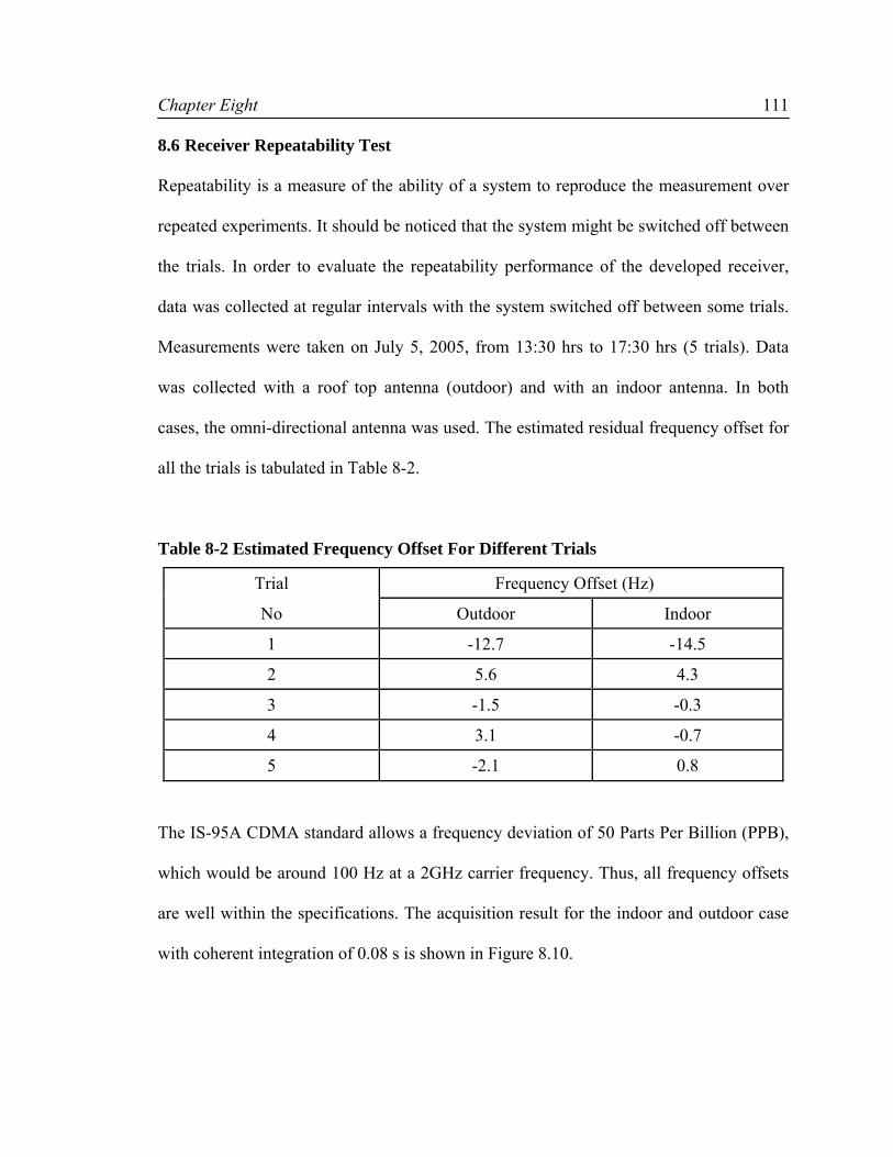
Chapter Eight
111
8.6 Receiver Repeatability Test
Repeatability is a measure of the ability of a system to reproduce the measurement over
repeated experiments. It should be noticed that the system might be switched off between
the trials. In order to evaluate the repeatability performance of the developed receiver,
data was collected at regular intervals with the system switched off between some trials.
Measurements were taken on July 5, 2005, from 13:30 hrs to 17:30 hrs (5 trials). Data
was collected with a roof top antenna (outdoor) and with an indoor antenna. In both
cases, the omni-directional antenna was used. The estimated residual frequency offset for
all the trials is tabulated in Table 8-2.
Table 8-2 Estimated Frequency Offset For Different Trials
Trial Frequency Offset (Hz)
No Outdoor Indoor
1 -12.7 -14.5
2 5.6 4.3
3 -1.5 -0.3
4 3.1 -0.7
5 -2.1 0.8
The IS-95A CDMA standard allows a frequency deviation of 50 Parts Per Billion (PPB),
which would be around 100 Hz at a 2GHz carrier frequency. Thus, all frequency offsets
are well within the specifications. The acquisition result for the indoor and outdoor case
with coherent integration of 0.08 s is shown in Figure 8.10.
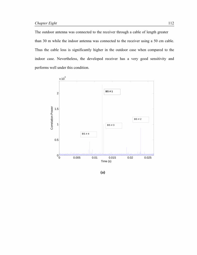
Chapter Eight
112
The outdoor antenna was connected to the receiver through a cable of length greater
than 30 m while the indoor antenna was connected to the receiver using a 50 cm cable.
Thus the cable loss is significantly higher in the outdoor case when compared to the
indoor case. Nevertheless, the developed receiver has a very good sensitivity and
performs well under this condition.
0 0.005 0.01 0.015 0.02 0.0250
0.5
1
1.5
2
x 104
Time (s)
Cor
rela
tion
Pow
er
BS # 1BS # 1
BS # 4
BS # 2
BS # 3
(a)

Chapter Eight
113
0 0.005 0.01 0.015 0.02 0.0250
2000
4000
6000
8000
10000
12000
Time (s)
Cor
rela
tion
Pow
erBS # 1
BS # 4
BS # 3
BS # 2
(b)
Figure 8.10 Acquisition with 0.08 s Coherent Integration (a) Outdoor Antenna (b)
Indoor Antenna
From the above acquisition plot, we can observe that BS # 1, BS # 2 and BS # 3 were
seen by both the indoor and outdoor antennas. The BS # 4 was different in both cases.
The BS # 4, observed by the outdoor antenna is not as strong as the BS # 4 observed by
the indoor antenna. While the indoor antenna faced shadowing, it was connected to the
receiver with cable of length of 50 cm. Thus, the cable loss is negligible in the case of the
indoor antenna when compared to the outdoor antenna.
The repeatability analysis in terms of range error for both the outdoor antenna and the
indoor antenna are tabulated in Table 8-3 and Table 8-4 respectively.
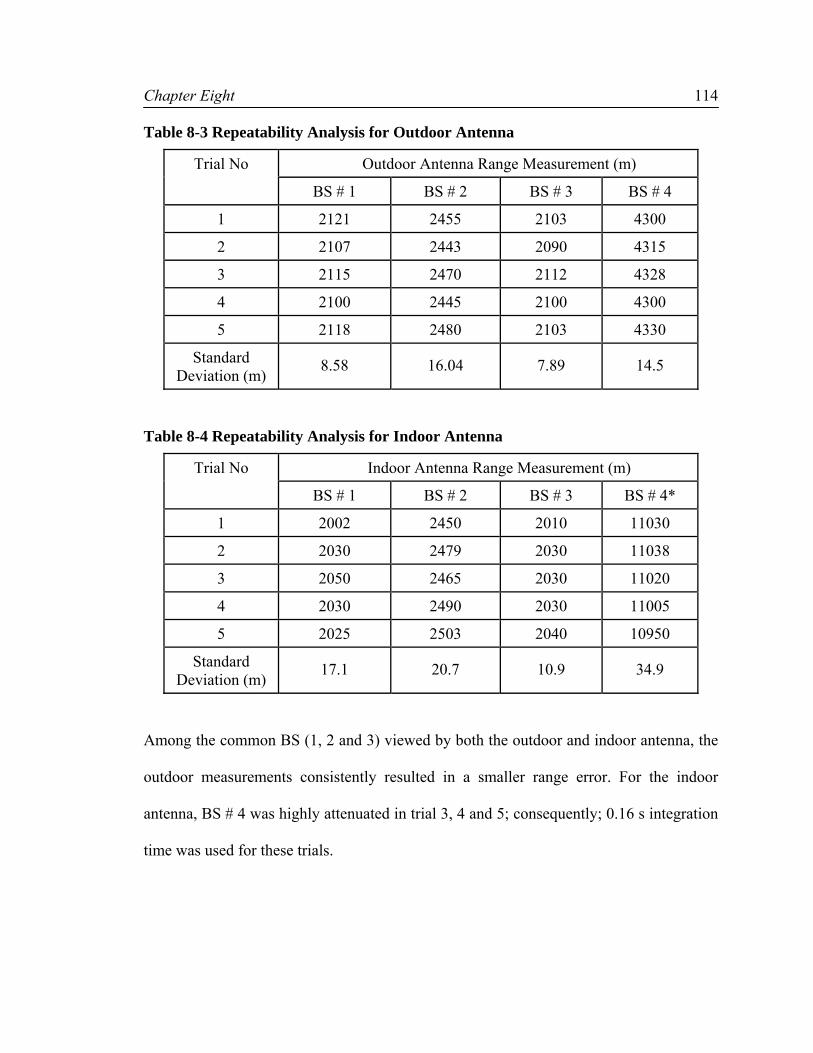
Chapter Eight
114
Table 8-3 Repeatability Analysis for Outdoor Antenna
Trial No Outdoor Antenna Range Measurement (m)
BS # 1 BS # 2 BS # 3 BS # 4
1 2121 2455 2103 4300
2 2107 2443 2090 4315
3 2115 2470 2112 4328
4 2100 2445 2100 4300
5 2118 2480 2103 4330
Standard Deviation (m) 8.58 16.04 7.89 14.5
Table 8-4 Repeatability Analysis for Indoor Antenna
Trial No Indoor Antenna Range Measurement (m)
BS # 1 BS # 2 BS # 3 BS # 4*
1 2002 2450 2010 11030
2 2030 2479 2030 11038
3 2050 2465 2030 11020
4 2030 2490 2030 11005
5 2025 2503 2040 10950
Standard Deviation (m) 17.1 20.7 10.9 34.9
Among the common BS (1, 2 and 3) viewed by both the outdoor and indoor antenna, the
outdoor measurements consistently resulted in a smaller range error. For the indoor
antenna, BS # 4 was highly attenuated in trial 3, 4 and 5; consequently; 0.16 s integration
time was used for these trials.
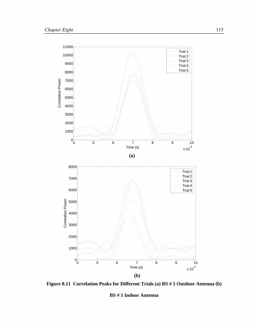
Chapter Eight
115
4 5 6 7 8 9 10
x 10-6
0
1000
2000
3000
4000
5000
6000
7000
8000
9000
10000
11000
Time (s)
Cor
rela
tion
Pow
er
Trial 1Trial 2Trial 3Trial 4Trial 5
(a)
4 5 6 7 8 9 10
x 10-6
0
1000
2000
3000
4000
5000
6000
7000
8000
Time (s)
Cor
rela
tion
Pow
er
Trial 1Trial 2Trial 3Trial 4Trial 5
(b)
Figure 8.11 Correlation Peaks for Different Trials (a) BS # 1 Outdoor Antenna (b)
BS # 1 Indoor Antenna

Chapter Eight
116
8.7 Field Tests
The outdoor field tests were primarily carried out to validate the performance of the
receiver. The field test was conducted at known GPS derived locations. The collected
data was processed in post-mission processing to analyze the receiver performance in
terms of accuracy and stability. The following sections describe the test methodology and
the resulting performance analysis.
8.7.1 Test Methodology
The test methodology involves the collection of the CDMA pilot signal from known
locations and then the processing of the collected data to analyze the performance of the
receiver. The position of the Base Stations as well as the identity of the service providers
who operate them were not known during the test. Thus, it was not possible to evaluate
the position accuracy performance of the receiver. Nevertheless, attempts were made to
investigate the position accuracy performance of the receiver in an indirect fashion. The
test methodology adopted for the data collection is summarized below.
• Choose two or more locations in such a way that these locations lie approximately
in the same baseline as the BS of interest.
• The distance from these measurement locations to the BS should be large (i.e. two
or more kilometres). In addition the range difference between these locations
should be much less than the range from the BS of interest.
• Survey these measurements location using DGPS and compute the range between
these positions independently with the sub-metre accuracy.

Chapter Eight
117
• Collect the CDMA data using the receiver at these known locations and then
process the data to compute the range difference between these locations.
• Compare the range differences (between these measurement locations) obtained
via DGPS with the receiver.
The outdoor field test setup for evaluation of the receiver accuracy performance is shown
in Figure 8.12.
Figure 8.12 Outdoor Field Test Setup
Three measurement locations were surveyed and their respective positions were
computed using DGPS. In order to evaluate the performance of the receiver in terms of
position accuracy, the position of the BS has to be known a priori. However, it is
possible to find the position of these measurement locations if the elevation angle of the
measurement locations to the BS antenna phase center is known.
D
D1 D2 D3
P1 P2 P3 d1 d2
d3

Chapter Eight
118
Figure 8.13 Path Delay between Two Measurement Locations
Instead of estimating the actual positions, the range difference between these
measurement locations can be estimated and then analyze them to investigate the receiver
performance.
Consider a hypothetical triangle as shown in Figure 8.13. The triangle is constructed by
drawing a perpendicular line between the paths that arrive from the BS of interest to the
two measurement locations P1 and P2. Since the two paths can be considered to be
parallel to each other the line subtended between these paths will be perpendicular as
well. To compute the range difference between these measurement locations and the BS
of interest, the path D2 – D1 and the angle θ should be known. Thus, the range difference
can be expressed as in (8.10),
( )θcos12
1
DDd
−= (8.10)
However, D>>d1, │D2 – D1│, (D is the distance from the BS of interest to the second
measurement location P2) the angle θ will tend towards zero. Thus,
d1 P1 P2
D2 – D1
θ
Base Station

Chapter Eight
119
121 DDd −= (8.11)
For this to hold true, both measurement locations must lie on the baseline as that of the
BS of interest. In other words, the difference in the angles subtended from the BS antenna
phase center and the phase centers of the antennas at the two measurement locations
should be negligible. Thus, the range difference can be computed between the two
locations using the TOA difference. This value converted to a unit of length and
compared to the DGPS derived distance between the two measurements locations, is a
measure of the consistency of the system and its uncorrelated noise.
8.7.2 Outdoor Field Test Specifications
The specifications of the outdoor field test are summarized below.
• Data was collected at three known locations. The position estimates of these
locations were computed separately using DGPS and then used to compute the
range difference between these measurement locations.
• The CDMA pilot signal was collected using two types of antennas (directional
and omni-directional antenna) with the receiver at each measurement locations.
• For each antenna at each measurement location, 8 seconds of data was collected.
• The data was collected at both carrier frequencies, 1947.5 MHz and 1981.25
MHz.
• Data was collected at these measurement locations at 15:10, 15:30 and 15:50 hrs
mountain standard time respectively. The ambient temperature was approximately
-8o C during the test.

Chapter Eight
120
• The directional antenna was oriented towards the BS which was situated near
the Canada Olympic Park. The receiver was located in a parking lot in front the
Calgary Centre for Innovative Technology (CCIT) building on the University of
Calgary campus, as shown in Figure 8.14.
Figure 8.14 Map Showing Measurement Locations
The time of the data collection is specified because of the variation of the pilot signal
power during the day. The ambient temperature is important because it will affect the
frequency offset.
8.7.3 Field Test Performance Analysis
The received data collected at these known locations was processed in post-mission
processing to obtain the approximate range measurement between the BS and these
measurement locations. The major issues that were observed from the post-mission
analysis are summarized below:
P1 P2
P3
Measurement Locations

Chapter Eight
121
• Preliminary analysis showed that the BS of interest was used by the carrier
TELUS (channel number N=350) at 1947.5 which was observed by both the
directional and the omni-directional antenna.
• The number of BS that could be observed was significantly low compared to the
earlier roof top antenna measurements. In almost all field test measurements, only
a few BS were observed.
• The number of BS observed by the directional and the omni-directional antennas
was similar.
• The TCXO had a significant residual frequency offset in the range of -600 to -800
Hz. The residual frequency offset for the different data sets are tabulated in Table
8-5. The resolution was 0.01 Hz and the predetection integration time was 0.08 s.
Table 8-5 Residual Frequency Offset for Outdoor Field Test
Frequency Offset (Hz)
Location Directional Antenna Omni-Directional Antenna
N=350
1947.5 MHz
N=1025
1981.25MHz
N=350
1947.5 MHz
N=1025
1981.25MHz
P1 -780.52 -768.67 -776.84 -805.32
P2 -685.09 -676.98 -651.35 -676.32
P3 -628.28 -657.58 -638.68 -652.08

Chapter Eight
122
The test antennas at location P1, P2 and P3 were only one to two metres above ground
level and this is the likely reason for the lower BS availability. In addition, all
measurement locations were surrounded by buildings of 3 or more storeys and this may
have significantly blocked the signal from a number of different BS. All of these factors
may also be responsible for similar BS availability as observed by the directional antenna
and the omni-directional antenna. The large frequency offset is caused by the low
ambient temperature at the measurement locations (the calibration of the Temperature
Compensated Crystal Oscillator was performed at room temperature).
8.7.4 Range Domain Analysis
The collected data sets were analyzed to find the correlation peak corresponding to the
BS of interest, which was in the direction of Canada Olympic Park. The BS of interest
was observed by both antennas at each of the measurement locations. The time offset
corresponding to the BS of interest at these locations was computed with a 0.08 s
coherent integration time and 0.1 chip resolution. The correlation peaks corresponding to
the three measurement locations for both the directional and the omni-directional antenna
are shown in Figure 8.15.

Chapter Eight
123
4 5 6 7 8 9 10 11 12
x 10-6
0
2000
4000
6000
8000
10000
12000
Time (s)
Cor
rela
tion
Pow
er
Directional Antenna
Pos 1Pos 2Pos 3
(a)
4 5 6 7 8 9 10 11 12
x 10-6
0
2000
4000
6000
8000
10000
12000
Time (s)
Cor
rela
tion
Pow
er
Omni-Directional Antenna
Pos 1Pos 2Pos 3
(b)
Figure 8.15 Correlation Peak of the BS of Interest at all Measurement Locations (a) Directional Antenna (b) Omni-Directional Antenna

Chapter Eight
124
Figure 8.15 shows that the time instants of the correlation peaks vary according to the
distance from the BS of interest to the location (i.e. D1 < D2 < D3). The correlation powers
observed by the omni-directional and the directional antennas were almost identical
despite of the fact that the directional antenna has a better antenna gain in that direction.
The exact TOA was estimated by taking the maximum value of the correlation peaks.
The approximate propagation delays computed for the measurement locations are given
in Table 8-6.
Table 8-6 Estimated Ranges
Antenna
Type
Measurements Position 1 Position 2 Position 3
Directional TProp (µs) 7.764 7.926 8.264
Antenna BS range (Km) 2.329 2.378 2.479
Omni-directional
TProp (µs) 8.014 8.176 8.502
Antenna BS range (Km) 2.404 2.453 2.551
The computed range measurements between the BS and the measurement locations are
different for the omni-directional and the directional antennas. This bias is caused by
antennas characteristics that are different for each antenna. The bias could be removed by
calibrating the antennas in an anechoic chamber. In the final system operating in pseudo-
TOA mode, that is in TOA mode with a receiver clock bias, an antenna bias of this type
will be absorbed by the receiver clock offset estimate.

Chapter Eight
125
Table 8-7 GPS and CDMA Receiver Computed Range Differences
P3 – P1 (m) P3 – P2 (m)
GPS Solutions ~151 ~101
Directional Antenna ~146.51 ~97.7
Omni-Directional Antenna ~146.46 ~97.65
Table 8-7 tabulates the range differences computed by the GPS solutions and the CDMA
Receiver using the two antennas.
From Table 8-7 it can be readily noticed that the receiver range differences are quite
accurate and agree within 10 m with the DGPS derived range differences. This would
imply a single measurement noise of 7 to 8 m prior to differentiation.
The range difference estimates were computed for the first epoch using 0.08 s coherent
integration intervals. Since there was no information available about the location of other
BS, a similar analysis was performed on other BS in order to confirm that the analyzed
BS was aligned with the measurement location; this resulted in wrong range difference
estimates.
8.8 Antenna Array
The angle of arrival of the received signal can be measured either by using an antenna
array or using directive antennas. An antenna array was selected to be used in this thesis.
The antenna array consist of 5-directional antennas azimuthally aligned, the antennas in
this array were equally spaced with distance d = 15.5 cm.
The number of antenna elements and the spacing d has a significant impact on the shape
of the radiation pattern of the array; the larger the number of antenna elements an array
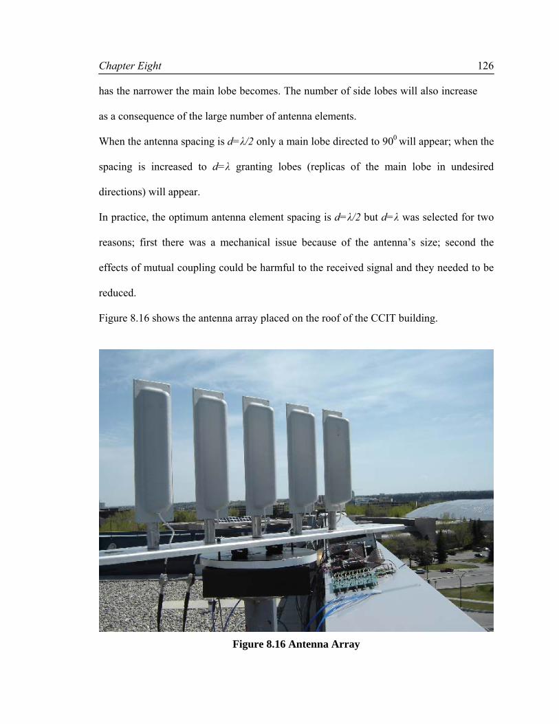
Chapter Eight
126
has the narrower the main lobe becomes. The number of side lobes will also increase
as a consequence of the large number of antenna elements.
When the antenna spacing is d=λ/2 only a main lobe directed to 900 will appear; when the
spacing is increased to d=λ granting lobes (replicas of the main lobe in undesired
directions) will appear.
In practice, the optimum antenna element spacing is d=λ/2 but d=λ was selected for two
reasons; first there was a mechanical issue because of the antenna’s size; second the
effects of mutual coupling could be harmful to the received signal and they needed to be
reduced.
Figure 8.16 shows the antenna array placed on the roof of the CCIT building.
Figure 8.16 Antenna Array
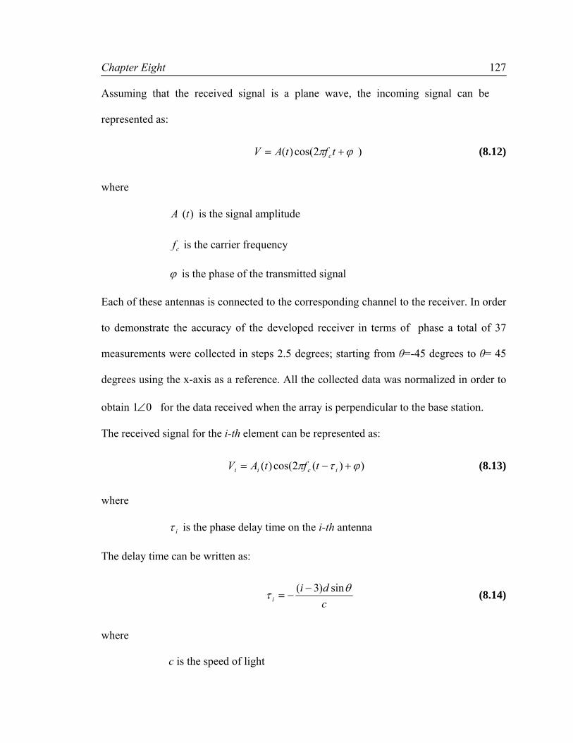
Chapter Eight
127
Assuming that the received signal is a plane wave, the incoming signal can be
represented as:
)2cos()( ϕπ += tftAV c (8.12)
where
)(tA is the signal amplitude
cf is the carrier frequency
ϕ is the phase of the transmitted signal
Each of these antennas is connected to the corresponding channel to the receiver. In order
to demonstrate the accuracy of the developed receiver in terms of phase a total of 37
measurements were collected in steps 2.5 degrees; starting from θ=-45 degrees to θ= 45
degrees using the x-axis as a reference. All the collected data was normalized in order to
obtain 01∠ for the data received when the array is perpendicular to the base station.
The received signal for the i-th element can be represented as:
))(2cos()( ϕτπ +−= icii tftAV (8.13)
where
iτ is the phase delay time on the i-th antenna
The delay time can be written as:
cdi
iθτ sin)3( −
−= (8.14)
where
c is the speed of light
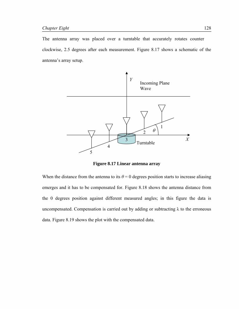
Chapter Eight
128
The antenna array was placed over a turntable that accurately rotates counter
clockwise, 2.5 degrees after each measurement. Figure 8.17 shows a schematic of the
antenna’s array setup.
Figure 8.17 Linear antenna array
When the distance from the antenna to its θ = 0 degrees position starts to increase aliasing
emerges and it has to be compensated for. Figure 8.18 shows the antenna distance from
the 0 degrees position against different measured angles; in this figure the data is
uncompensated. Compensation is carried out by adding or subtracting λ to the erroneous
data. Figure 8.19 shows the plot with the compensated data.
Incoming Plane Wave
X
Y
1 2
4 3
θ
Turntable
5

Chapter Eight
129
-50 -40 -30 -20 -10 0 10 20 30 40 50-0.25
-0.2
-0.15
-0.1
-0.05
0
0.05
0.1
0.15
0.2
0.25
Measured Angle in Degrees
Ant
enna
Dis
tanc
e fro
m 0
° pos
ition
in m
Channel 1Channel 2Channel 3Channel 4Channel 5
Figure 8.18 Uncompensated measured data
-50 -40 -30 -20 -10 0 10 20 30 40 50-0.25
-0.2
-0.15
-0.1
-0.05
0
0.05
0.1
0.15
0.2
0.25
Measured Angle in Degrees
Ant
enna
Dis
tanc
e fro
m 0
° pos
ition
in m
Channel 1Channel 2Channel 3Channel 4Channel 5
Figure 8.19 Compensated measured data
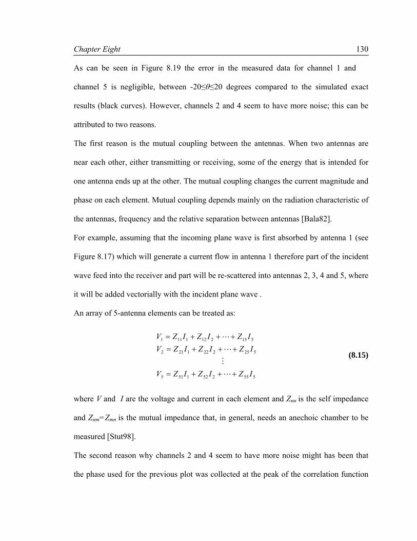
Chapter Eight
130
As can be seen in Figure 8.19 the error in the measured data for channel 1 and
channel 5 is negligible, between -20≤θ≤20 degrees compared to the simulated exact
results (black curves). However, channels 2 and 4 seem to have more noise; this can be
attributed to two reasons.
The first reason is the mutual coupling between the antennas. When two antennas are
near each other, either transmitting or receiving, some of the energy that is intended for
one antenna ends up at the other. The mutual coupling changes the current magnitude and
phase on each element. Mutual coupling depends mainly on the radiation characteristic of
the antennas, frequency and the relative separation between antennas [Bala82].
For example, assuming that the incoming plane wave is first absorbed by antenna 1 (see
Figure 8.17) which will generate a current flow in antenna 1 therefore part of the incident
wave feed into the receiver and part will be re-scattered into antennas 2, 3, 4 and 5, where
it will be added vectorially with the incident plane wave .
An array of 5-antenna elements can be treated as:
5552521515
5252221212
5152121111
IZIZIZV
IZIZIZVIZIZIZV
+++=
+++=+++=
L
M
L
L
(8.15)
where V and I are the voltage and current in each element and Znn is the self impedance
and Znm=Zmn is the mutual impedance that, in general, needs an anechoic chamber to be
measured [Stut98].
The second reason why channels 2 and 4 seem to have more noise might has been that
the phase used for the previous plot was collected at the peak of the correlation function
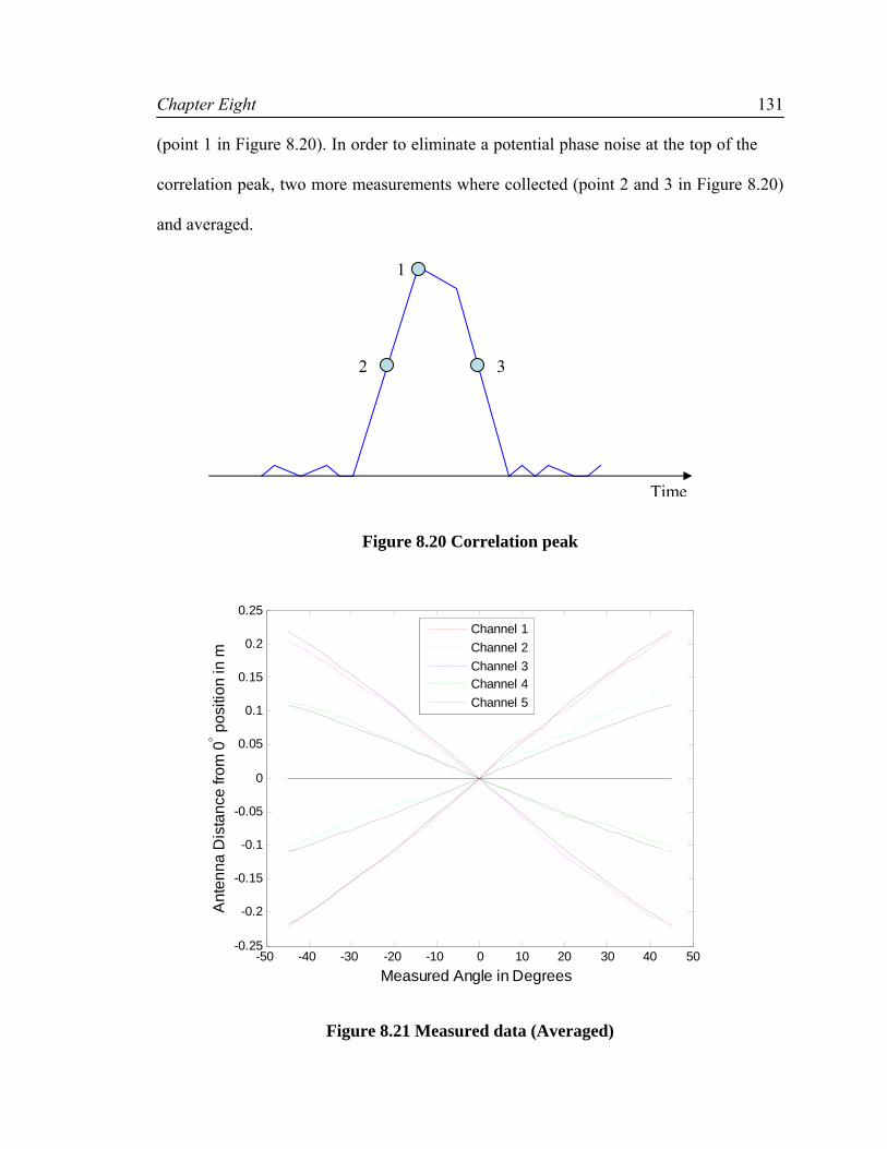
Chapter Eight
131
(point 1 in Figure 8.20). In order to eliminate a potential phase noise at the top of the
correlation peak, two more measurements where collected (point 2 and 3 in Figure 8.20)
and averaged.
Figure 8.20 Correlation peak
-50 -40 -30 -20 -10 0 10 20 30 40 50-0.25
-0.2
-0.15
-0.1
-0.05
0
0.05
0.1
0.15
0.2
0.25
Measured Angle in Degrees
Ant
enna
Dis
tanc
e fro
m 0
° pos
ition
in m
Channel 1Channel 2Channel 3Channel 4Channel 5
Figure 8.21 Measured data (Averaged)
2
Time
3
1

Chapter Eight
132
Figure 8.21 shows the averaged angle measurements; a slightly better result is shown
for channel 1 and channel 5; even though the performances of channels 2 and 3 are better
for certain angles measurements, the overall end result is slightly worse.
8.9 Angle of Arrival Measurements
The previous section showed the received signal for independent channels. There is a
wide variety of algorithms that can be used to estimate the AOA from the data obtained
by the antenna array such as MUSIC and ESPRIT. The analysis of these sophisticated
AOA methods of estimation will not be performed in this thesis.
By combining the independent measurements collected in the previous section; the Angle
of Arrival can be obtained by using a Least-Square method. In order to apply this method
it is necessary to assume:
• Perfect calibration (at θ = 0 , outputs normalized to 1 )
• Phase centers of array are analyzed (at θ = 0 array ⊥ K )
Figure 8.22 Linear Array Geometry
θ
d
K
P
1 2
3
4 5

Chapter Eight
133
As previously shown the Least-Square algorithm will determine θ using ( ) ( )θθ 51 ....VV
where the received signal can be written as:
)( iPKji eV •−= (8.16)
where
⎥⎦
⎤⎢⎣
⎡=
0/2 λπ
K (8.17)
is the incoming plane wave and
( )( ) ⎥
⎦
⎤⎢⎣
⎡−−=
θθ
cossin
)3(idPi (8.18)
is the position of the i-th antenna. Substituting (8.17) and (8.18) into (8.16), results in
)sin()3(2θ
λπ
−=
idj
i eV (8.19)
Equations (8.20) and (8.21) can be obtained by finding the real and imaginary part of
equation (8.19);
( ) ( )⎟⎠⎞
⎜⎝⎛ −== θλπ sin32cos)( idVreale ii (8.20)
( ) ( )⎟⎠⎞
⎜⎝⎛ −== θλπ sin32sin)( idVimagg ii (8.21)
The least square solution is given by:
))(()( 1Old
TT MMJJJ θθ −=Δ − (8.22)

Chapter Eight
134
where M is actual normalized measurements
⎥⎥⎥⎥⎥⎥⎥
⎦
⎤
⎢⎢⎢⎢⎢⎢⎢
⎣
⎡
=
5
1
5
1
g
ge
e
M
M
M
(8.23)
And J represents the Jacobian matrix
⎥⎥⎥
⎦
⎤
⎢⎢⎢
⎣
⎡=
5
1
J
JJ M
( ) ( ) ( ) ( )
( ) ( ) ( ) ( )⎥⎥⎥⎥
⎦
⎤
⎢⎢⎢⎢
⎣
⎡
−⎟⎠⎞
⎜⎝⎛ −−
−⎟⎠⎞
⎜⎝⎛ −
=⎥⎥⎥
⎦
⎤
⎢⎢⎢
⎣
⎡
∂∂∂∂
−=θ
λπθ
λπ
θλπθ
λπ
θ
θ
cos32sin32cos
cos32sin32sin
idid
idid
g
e
Ji
i
i (8.24)
-50 -40 -30 -20 -10 0 10 20 30 40 50-50
-40
-30
-20
-10
0
10
20
30
40
50
Turntable Angle in degrees
Est
imat
ed A
ngle
in d
egre
es
Measured AngleSimulated Exact Result
Figure 8.23 LS Results
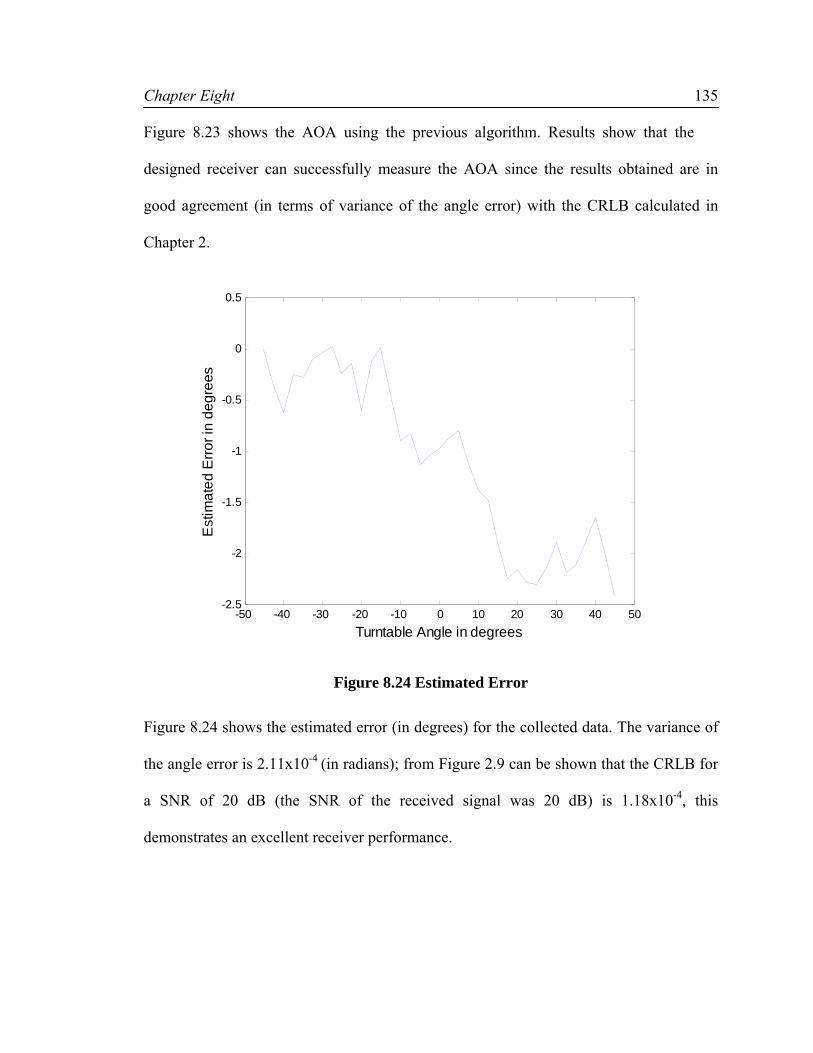
Chapter Eight
135
Figure 8.23 shows the AOA using the previous algorithm. Results show that the
designed receiver can successfully measure the AOA since the results obtained are in
good agreement (in terms of variance of the angle error) with the CRLB calculated in
Chapter 2.
-50 -40 -30 -20 -10 0 10 20 30 40 50-2.5
-2
-1.5
-1
-0.5
0
0.5
Turntable Angle in degrees
Est
imat
ed E
rror i
n de
gree
s
Figure 8.24 Estimated Error
Figure 8.24 shows the estimated error (in degrees) for the collected data. The variance of
the angle error is 2.11x10⁻⁴ (in radians); from Figure 2.9 can be shown that the CRLB for
a SNR of 20 dB (the SNR of the received signal was 20 dB) is 1.18x10⁻⁴, this
demonstrates an excellent receiver performance.

Chapter Nine
136
CHAPTER NINE: CONCLUSIONS AND FUTURE WORK
9.1 Conclusions
• This thesis presented a complete 5-channel design and implementation of a
CDMA receiver capable of making the necessary pilot signal measurements to be
used in TOA and AOA positioning.
• Due to its high signal-to-noise ratio and phase stability, the designed receiver
proved to be suitable for TOA and AOA measurements.
• This thesis also surveyed different receiver architectures that are suitable for this
application, as well as discussed the advantages and disadvantages of each of
these architectures.
• It was found that the frequency offset greatly affect the Signal to Noise Ratio and
that this frequency offset has to be eliminated in order to have accurate
measurements.
• It was shown that the receiver needs to be accurately calibrated in order to avoid
IM distortion.
• AOA accuracy achieved was ~1o across a sweep of 90o
9.2 Future Work
The work presented in this thesis can be extended in many ways among them:
• A more sophisticated analysis of the influence of oscillator’s accuracy for Time
of Arrival measurements can be done.
Chapter Nine
137
• If size reduction of the receiver is needed; an implementation of a direct
conversion receiver or a low IF receiver should be considered, even though they
have some disadvantages they will greatly reduce the size of the receiver.
• Additional research is needed to evaluate the performance of the receiver in
NLOS situations.
• Another avenue of progress may be the study of different ways of combining
information when more than one position location method is used to locate the
mobile such as the combination of AOA /TOA or AOA/TDOA methods.
• The influence of mutual coupling in Angle of Arrival measurements has to be
studied in more detail; data collection using different types of antennas (omni-
directional antennas) is a good start.
• Outdoor positioning with stationary platform in different environments should be
performed.
• Indoor positioning in environment of poor SNR should be performed.
• Other factors limiting long integration times should be explored. Long integration
times are needed for detection of weak signals.

References
138
References
[Alia00] Ali-Ahmad, W. W., “The CDMA Receiver System in an IS-98-A Standard”, RF
System Design, Electronics Engineer, 2000.
[Bala82] C. A. Balanis, “Antenna Theory, Analysis and Design”, Second Edition, John
Wiley & Sons, Inc, 1997.
[Bess03I] L. Besser, R. Gilmore, “Practical RF Circuit Design for Modern Wireless
Systems, Passive Circuits and Systems” Volume I, Artech House Microwave
Library, 2003.
[Bess03II] L. Besser, R. Gilmore, “Practical RF Circuit Design for Modern Wireless
Systems, Active Circuits and Systems” Volume II, Artech House Microwave
Library, 2003.
[Blank98] T. K. Blankenship, “Design and Implementation of a Pilot Signal Scanning
Receiver for CDMA Personal Communication Services System”, M. S. Thesis,
Virginia Polytechnic Institute, 1998.
[Caff98] J. J. Caffery Jr., G. L. Stuber, “Overview of Radiolocation in CDMA Cellular
Systems”, Communication Magazine IEEE, Vol. 36, April 1998.
[Caffe98] J. J. Caffery Jr., G. L. Stuber, “Subscriber Location in CDMA Cellular
Networks”, IEEE Transaction on Vehicular Technology, Vol. 47, No 2 May
1998.
[Caff00] J. J. Caffery Jr., “Wireless Location in CDMA Cellular Radio Systems”, Kluwer
Academic Publisher, 2000.
[Chan01] K. Chang, I. Bahl, V. Nair, “RF and Microwave Circuit and Components
Design for Wireless Systems”, John Wiley & Sons, 2001.
References
139
[Chen97] S. Chen, “Linearity Requirements for Digital Wireless Communications”,
IEEE Transaction, 1997
[Egan03] W. F. Egan, “Practical RF Systems”, John Wiley & Sons, 2003.
[Garg97] V. K. Garg, K. Smolik, J. E. Wilkes, “Applications of CDMA in Wireless /
Personal Communications”, Prentice Hall, 1997.
[Gray95] P. R. Gray, R. G. Meyer, “Future Directions in Silicon ICs for Personal
Communications”, Custom Integrated Circuits Conference, 1995.
[Heps99] E. Hepsaydir, “Mobile Positioning in CDMA Cellular Networks”, Vehicular
Technology Conference, IEEE VTS 50th, Volume 2, Sept. 1999.
[Kay98] S. M. Kay, “Fundamentals of Statistical Signal Processing: Estimation
Theory”, Prentice Hall, 1998.
[Kim05] J. Kim, D. Devries, “Measuring Single-Tone Desensitization for CDMA
Receivers”, Next-Generation Wireless, RF Design, 2005.
[Kluk97] R. W. Klukas, “A Superresolution Based Cellular Positioning System Using
GPS Time Synchronization”, Ph. D. Thesis, University of Calgary, 1997.
[Kuhn95] W. B. Kuhn, “Design of Integrated, Low Power, Radio Receivers in BiCMOS
Technologies”, Ph. D. Thesis, Virginia Polytechnic Institute and State
University, 1995.
[Lee98] J. S. Lee, L. E. Miller, “CDMA System Engineering Handbook”, Artech House,
1998.
[Leun02] B. Leung, “VLSI for Wireless Communication”, Prentice Hall Electronics and
VLSI Series, 2002.

References
140
[Lope05] A. Lopez, D. Lu, S. Shanmugam, C. Ma, J. Nielsen, R. Klukas, G.
Lachapelle, “Tactical Outdoor Positioning System Development”, Progress
Report for DRDC, Department of National Defence, Ottawa, pages 68, 2005.
[Lu05] D. Lu, A. Lopez, S. K. Shanmugam, J. Nielsen, G. Lachapelle, “Phase Coherency
of CDMA Caller Location Processing Based on TCXO Frequency Reference
with Intermittent GPS Correction”, Wireless Conference, 2005.
[Ma03] C. Ma, “Technique to Improve Ground-Based Wireless Location Performance
Using Cellular Telephone Network”, Ph. D. Thesis, University of Calgary,
2003.
[Messi98] G. G. Messier, M. Fattouche, B. R. Petersen, “Locating an IS-95 Mobile Using
Its Signal”, The Tenth International Conference on Wireless Communications,
Vol. II, July 1998.
[Rhee98] M. Y. Rhee, “CDMA Cellular Mobile Communications, Network & Security”,
Prentice Hall, 1998.
[Poza01] D. M. Pozar, “Microwave and RF Design of Wireless Systems”, John Wiley &
Sons Inc, 2001.
[Poza05] D. M. Pozar, “Microwave Engineering”, Third Edition, John Wiley & Sons
Inc, 2005.
[Rapp96] T. S. Rappaport, J. H. Reed, B. D. Woerner, “Position Location Using Wireless
Communication on Highways of the Future”, Communication Magazine,
IEEE, Volume 34, Issue 10, Oct. 1996.
[Rapp02] T. S. Rappaport, “Wireless Communications, Principle and Practice”, Prentice
Hall, 2002.

References
141
[Rohd01] U. Rohde, J. Whitaker, “Communication Receivers, DSP, Software Radio
and Design”, Third Edition, Mac Graw Hill, 2001.
[Rude97] J. C. Rudell, J. Ou, T. Byunghak Cho, G. Chien, F. Brianti, J. A. Weldon,
P.Gray, “A 1.9-GHz Wide-Band IF Double Conversion CMOS Receiver For
Cordless Telephone Applications”, IEEE Journal of Solid States Circuits, Vol.
32, No 12, 1997.
[Rude98] J. C. Rudell, J. Ou, R. Sekhar Narayanaswami, G. Chien, J. A. Weldon, L. Lin,
K. Tsai, L.Tee, K. Khoo, D. Au, T. Robison, D. Gerna, M. Otsuka, P.Gray,
“Recent Developments in High Integration Multi-Standard CMOS
Transceivers for Personal Communication Systems”, International Symposium
on Low Power Electronics and Design, 1998.
[Saye03] A. H. Sayed, N. R. Yousef, “Wireless Location”, Wiley Encyclopedia of
Telecommunications, Wiley & Sons, 2003.
[Saye05] A. H. Sayed, A. Tarighat, N. Khajehnouri, “Network-Based Wireless Location”,
IEEE Signal Processing Magazine, 2005.
[Shan05] S. K. Shanmugam, A. Lopez, D. Lu, N. Luo, J. Nielsen, G. Lachapelle, R.
Klukas, A. Taylor, “Wireless Location in IS-95 CDMA Cellular Radio
System”, Wireless Conference, 2005.
[Stut98] W. L. Stutzman, G. A. Thiele, “Antenna Theory and Design”, Second Edition,
John Wiley & Sons, Inc, 1998.
[Sun04] Y. Sun, “Wireless Communication Circuits and Systems”, IEE Circuits,
Devices and Systems Series, 2004.

References
142
[Texa99] Technical Brief, “Understanding and Enhancing Sensitivity in Receivers for
Wireless Aplications”, Texas Instrument, 1999.
[TIA/EIA00] TIA/EIA Interim Standard, CDMA 2000 series, Telecommunication
Industry Association, 1999.
[Meht01] J. L. Mehta, “Transceiver Architectures for Wireless ICs”, RF Design
Magazine, 2001.
[Morl95] G. D. Morley, “Improved Location Estimation for Automatic Vehicle
Monitoring with Multipath-Corrupted Range Measurements”, Master of
Engineering Thesis, University of Alberta, 1995.
[Vard00] G. Vardoulias, “Receiver Synchronization Techniques for CDMA Mobile Radio
Communications based on the use of A Priori Information”, Ph. D. Thesis, The
University of Edinburgh, September 2000.
[Yaco02] M. D. Yacoub, “Wireless Technology, Protocols, Standards and Techniques”,
CRC Press, 2002.
[Zhao00] Y. Zhao, “Mobile Phone Location Determination and Its Impact on Intelligent
Transportation Systems”, IEEE Transactions on Intelligent Transportation
Systems, Vol. 1, No. 32, March 2000.