university of calgary geopotential of the geoid...
TRANSCRIPT
UNIVERSITY OF CALGARY
Geopotential of the Geoid-Based North American Vertical Datum
by
Tasnuva Tahia Hayden
A THESIS
SUBMITTED TO THE FACULTY OF GRADUATE STUDIES
IN PARTIAL FULFILMENT OF THE REQUIREMENTS FOR THE
DEGREE OF MASTER OF SCIENCE
DEPARTMENT OF GEOMATICS ENGINEERING
CALGARY, ALBERTA
JULY, 2013
© Tasnuva Tahia Hayden
ii
ABSTRACT
The European Space Agency’s dedicated satellite gravity field mission the Gravity Field
and Steady-state Ocean Circulation Explorer (GOCE) will at the end of its lifespan
achieve 1-2 cm geoid accuracy at a spatial resolution of 100 km. This thesis attempts to
answer the question: is a GOCE satellite-only global geopotential model (GGM)
sufficient for geodetic applications such as datum unification in North America? The
main research objectives that were investigated in order to answer this question include:
GOCE GGM evaluation, estimation of height datum offsets for regional vertical datums,
and the estimation of the gravity potential for a geoid-based vertical datum. Based on the
research objective outcomes, it can be concluded that using only a GOCE satellite-based
GGM is not sufficient for geodetic applications such as datum unification in North
America. Thus, a GOCE GGM should be rigorously combined with gravity and
topography data in a remove-compute-restore geoid modelling scheme.
iii
ACKNOWLEDGEMENTS
I would like to express my sincere thanks to my supervisor, Dr. Michael G. Sideris, for
his supervision and support over the past two and a half years. His knowledge and
recommendations on a large variety of topics from how to give effective presentations,
how to improve my journal papers and thesis, and even how to better my teaching and
instructional skills, have been invaluable and much appreciated.
I would also like to thank the very beautiful and intelligent, Dr. Elena Rangelova, whose
guidance and friendship has enhanced my time at University of Calgary. Really, this
thesis, the journal papers, and even Advanced Physical Geodesy (which has left a scar on
my heart) would not have been as successfully completed without her help. Elena, this
must be said: you are a strong role model for women wishing to pursue further studies
and a career in the sciences.
Next, I would like to thank my dear friend and colleague, Babak Amjadiparvar, for all the
stimulating discussions we have had during the preparation of this thesis. Without his
help in many matters, I am not sure how this thesis would have ever seen the “light at the
end of the tunnel”. Truly, he cannot be thanked enough!
Marc Véronneau at the Geodetic Survey Division of Natural Resources Canada is
acknowledged for providing me with various datasets, collaborating on journal papers,
and for always taking the time to answer my questions. By the same token, the staff at the
Canadian Hydrographic Service are thanked for their prompt responses to my questions,
as well as Dan Roman from the U.S.A. National Geodetic Survey, and Jianliang Huang
from the Geodetic Survey Division of Natural Resources Canada. P. Woodworth and C.
Hughes are acknowledged for providing me with ten different global sea surface
topography models that have been utilized in this thesis. The late D.G. Wright is
acknowledged for the development of the regional Atlantic sea surface topography model
utilized in this study. Last but not least, Sinem Ince is acknowledged for providing a
gravimetric geoid model of Canada that has been used in this study.
iv
A genuine thank you goes to my graduate committee, which consisted of Dr. J.W. Kim,
Dr. Patrick Wu, and Dr. Kyle O’Keefe, for their feedback and constructive comments,
which has considerably improved the final version of this thesis.
Finally, I would like to give a big shout out of gratitude to my family and friends for their
unconditional love and support. The other graduate students in the gravity and earth
observations group are thanked for their friendship. In particular, I would like to thank
my office mate, Feng Tang, for providing me with data and helping me to debug C++
code for two course projects, and Jin Baek, for all the pep talks when I really just wanted
to call it quits.
This work is a contribution to the ESA STSE – GOCE+ Height System Unification with
GOCE project, and was also supported by NSERC, GEOIDE Network Centres of
Excellence, Queen Elizabeth II scholarship, and by graduate scholarships and teaching
assistantships from the University of Calgary.
v
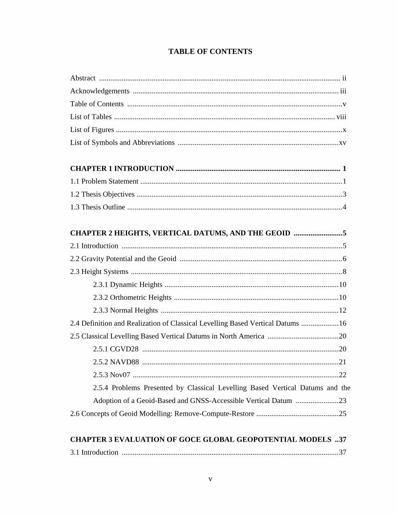
TABLE OF CONTENTS
Abstract ................................................................................................................................. ii
Acknowledgements .............................................................................................................. iii
Table of Contents ................................................................................................................... v
List of Tables ...................................................................................................................... viii
List of Figures ......................................................................................................................... x
List of Symbols and Abbreviations ...................................................................................... xv
CHAPTER 1 INTRODUCTION ........................................................................................ 1
1.1 Problem Statement ............................................................................................................ 1
1.2 Thesis Objectives .............................................................................................................. 3
1.3 Thesis Outline ................................................................................................................... 4
CHAPTER 2 HEIGHTS, VERTICAL DATUMS, AND THE GEOID .......................... 5
2.1 Introduction ...................................................................................................................... 5
2.2 Gravity Potential and the Geoid ....................................................................................... 6
2.3 Height Systems ................................................................................................................. 8
2.3.1 Dynamic Heights ............................................................................................. 10
2.3.2 Orthometric Heights ........................................................................................ 10
2.3.3 Normal Heights ............................................................................................... 12
2.4 Definition and Realization of Classical Levelling Based Vertical Datums .................... 16
2.5 Classical Levelling Based Vertical Datums in North America ...................................... 20
2.5.1 CGVD28 ......................................................................................................... 20
2.5.2 NAVD88 ......................................................................................................... 21
2.5.3 Nov07 .............................................................................................................. 22
2.5.4 Problems Presented by Classical Levelling Based Vertical Datums and the
Adoption of a Geoid-Based and GNSS-Accessible Vertical Datum ....................... 23
2.6 Concepts of Geoid Modelling: Remove-Compute-Restore ............................................ 25
CHAPTER 3 EVALUATION OF GOCE GLOBAL GEOPOTENTIAL MODELS .. 37
3.1 Introduction .................................................................................................................... 37
vi
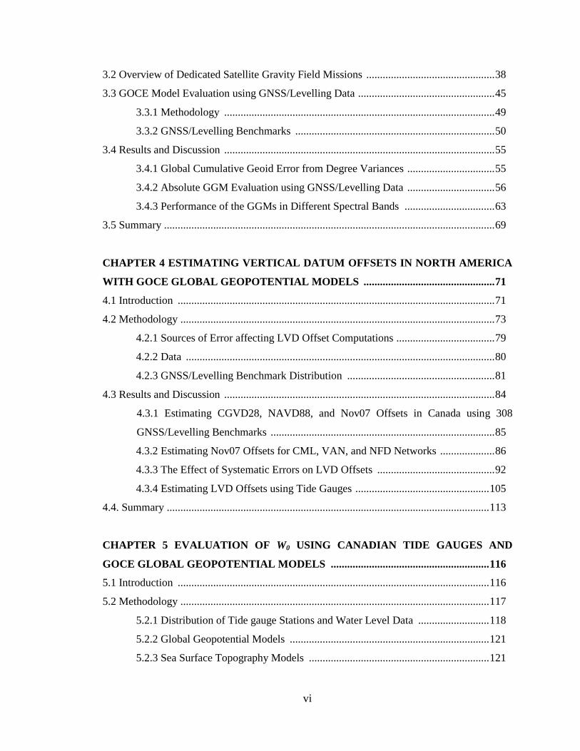
3.2 Overview of Dedicated Satellite Gravity Field Missions ............................................... 38
3.3 GOCE Model Evaluation using GNSS/Levelling Data .................................................. 45
3.3.1 Methodology ................................................................................................... 49
3.3.2 GNSS/Levelling Benchmarks ......................................................................... 50
3.4 Results and Discussion ................................................................................................... 55
3.4.1 Global Cumulative Geoid Error from Degree Variances ................................ 55
3.4.2 Absolute GGM Evaluation using GNSS/Levelling Data ................................ 56
3.4.3 Performance of the GGMs in Different Spectral Bands ................................. 63
3.5 Summary ......................................................................................................................... 69
CHAPTER 4 ESTIMATING VERTICAL DATUM OFFSETS IN NORTH AMERICA
WITH GOCE GLOBAL GEOPOTENTIAL MODELS ................................................ 71
4.1 Introduction .................................................................................................................... 71
4.2 Methodology ................................................................................................................... 73
4.2.1 Sources of Error affecting LVD Offset Computations .................................... 79
4.2.2 Data ................................................................................................................. 80
4.2.3 GNSS/Levelling Benchmark Distribution ...................................................... 81
4.3 Results and Discussion ................................................................................................... 84
4.3.1 Estimating CGVD28, NAVD88, and Nov07 Offsets in Canada using 308
GNSS/Levelling Benchmarks .................................................................................. 85
4.3.2 Estimating Nov07 Offsets for CML, VAN, and NFD Networks .................... 86
4.3.3 The Effect of Systematic Errors on LVD Offsets ........................................... 92
4.3.4 Estimating LVD Offsets using Tide Gauges ................................................. 105
4.4. Summary ...................................................................................................................... 113
CHAPTER 5 EVALUATION OF W0 USING CANADIAN TIDE GAUGES AND
GOCE GLOBAL GEOPOTENTIAL MODELS .......................................................... 116
5.1 Introduction .................................................................................................................. 116
5.2 Methodology ................................................................................................................. 117
5.2.1 Distribution of Tide gauge Stations and Water Level Data .......................... 118
5.2.2 Global Geopotential Models ......................................................................... 121
5.2.3 Sea Surface Topography Models .................................................................. 121
vii
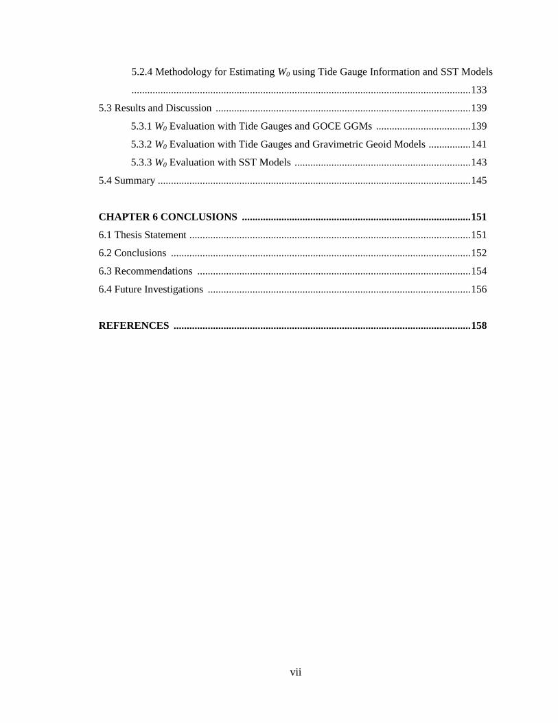
5.2.4 Methodology for Estimating W0 using Tide Gauge Information and SST Models
................................................................................................................................. 133
5.3 Results and Discussion ................................................................................................. 139
5.3.1 W0 Evaluation with Tide Gauges and GOCE GGMs .................................... 139
5.3.2 W0 Evaluation with Tide Gauges and Gravimetric Geoid Models ................ 141
5.3.3 W0 Evaluation with SST Models ................................................................... 143
5.4 Summary ....................................................................................................................... 145
CHAPTER 6 CONCLUSIONS ....................................................................................... 151
6.1 Thesis Statement ........................................................................................................... 151
6.2 Conclusions .................................................................................................................. 152
6.3 Recommendations ........................................................................................................ 154
6.4 Future Investigations .................................................................................................... 156
REFERENCES ................................................................................................................. 158
viii
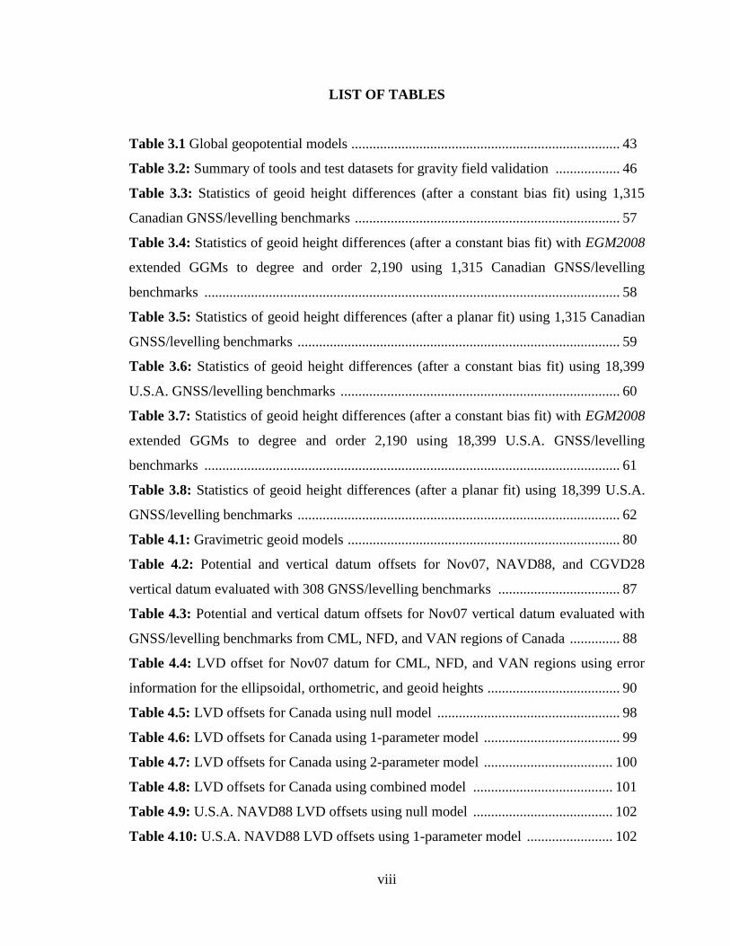
LIST OF TABLES
Table 3.1 Global geopotential models ........................................................................... 43
Table 3.2: Summary of tools and test datasets for gravity field validation .................. 46
Table 3.3: Statistics of geoid height differences (after a constant bias fit) using 1,315
Canadian GNSS/levelling benchmarks .......................................................................... 57
Table 3.4: Statistics of geoid height differences (after a constant bias fit) with EGM2008
extended GGMs to degree and order 2,190 using 1,315 Canadian GNSS/levelling
benchmarks .................................................................................................................... 58
Table 3.5: Statistics of geoid height differences (after a planar fit) using 1,315 Canadian
GNSS/levelling benchmarks .......................................................................................... 59
Table 3.6: Statistics of geoid height differences (after a constant bias fit) using 18,399
U.S.A. GNSS/levelling benchmarks .............................................................................. 60
Table 3.7: Statistics of geoid height differences (after a constant bias fit) with EGM2008
extended GGMs to degree and order 2,190 using 18,399 U.S.A. GNSS/levelling
benchmarks .................................................................................................................... 61
Table 3.8: Statistics of geoid height differences (after a planar fit) using 18,399 U.S.A.
GNSS/levelling benchmarks .......................................................................................... 62
Table 4.1: Gravimetric geoid models ............................................................................ 80
Table 4.2: Potential and vertical datum offsets for Nov07, NAVD88, and CGVD28
vertical datum evaluated with 308 GNSS/levelling benchmarks .................................. 87
Table 4.3: Potential and vertical datum offsets for Nov07 vertical datum evaluated with
GNSS/levelling benchmarks from CML, NFD, and VAN regions of Canada .............. 88
Table 4.4: LVD offset for Nov07 datum for CML, NFD, and VAN regions using error
information for the ellipsoidal, orthometric, and geoid heights ..................................... 90
Table 4.5: LVD offsets for Canada using null model ................................................... 98
Table 4.6: LVD offsets for Canada using 1-parameter model ...................................... 99
Table 4.7: LVD offsets for Canada using 2-parameter model .................................... 100
Table 4.8: LVD offsets for Canada using combined model ....................................... 101
Table 4.9: U.S.A. NAVD88 LVD offsets using null model ....................................... 102
Table 4.10: U.S.A. NAVD88 LVD offsets using 1-parameter model ........................ 102
ix
Table 4.11: U.S.A. NAVD88 LVD offsets using 2-parameter model ........................ 102
Table 4.12: U.S.A. NAVD88 LVD offsets using combined model ............................ 103
Table 4.13: CML LVD offsets computed by removing systematic effects from raw geoid
height residuals before the estimation of the offset using various parametric models ......
....................................................................................................................................... 103
Table 4.14: U.S.A. NAVD88 LVD offsets computed by removing systematic effects
from raw geoid height residuals before the estimation of the offset using various
parametric models ........................................................................................................ 104
Table 4.15: CGVD28 offset with 16 Canadian tide gauges ........................................ 109
Table 4.16: CGVD28 offset with 12 Canadian tide gauges ........................................ 109
Table 4.17: CGVD28 offset with 2 Canadian tide gauges (Atlantic) ......................... 110
Table 4.18: CGVD28 offset with 5 Canadian tide gauges (Pacific) ........................... 110
Table 4.19: NAVD88 offset with 59 U.S.A. tide gauges ............................................ 112
Table 4.20: NAVD88 offset with 28 U.S.A. tide gauges (Atlantic) ........................... 112
Table 4.21: NAVD88 offset with 18 U.S.A. tide gauges (Pacific) ............................. 112
Table 4.22: NAVD88 offset with 13 U.S.A. tide gauges (Gulf) ................................. 112
Table 5.1: Canadian tide gauge stations and local mean sea levels at epoch 2008.0 . 120
Table 5.2: Comparison of geometrically determined SST at tide gauge with CGG2010
and SST interpolated to tide gauge station locations from various SST models ......... 129
Table 5.3: W0 values for Pacific and Atlantic tide gauges with 19 years of water level
data with GGMs expanded to degree and order 180 and 2,190 (add 62,636,800.00 m2/s
2
to values in table) ......................................................................................................... 139
Table 5.4: W0 values evaluated using Pacific and Atlantic tide gauges with 19 years of
water level data and different gravity field models (add 62,636,800.00 m2/s
2 to values in
the table) ....................................................................................................................... 140
Table 5.5: W0 values for three Canadian regions computed with regional gravimetric
geoid models (add 62,636,800.00 m2/s
2 to all values) ................................................. 142
Table 5.6: W0 values evaluated with SST interpolated from models at tide gauges ... 143
Table 5.7: W0 values evaluated for the Pacific and Atlantic oceans using SST models ...
....................................................................................................................................... 147
x
LIST OF FIGURES
Figure 2.1: Ellipsoidal (hP) and orthometric (H(j)
P) heights ............................................ 6
Figure 2.2: Normal heights (Hnorm(j)
P), height anomaly (ξP), quasi-geoid and local quasi-
geoid ............................................................................................................................... 15
Figure 2.3: Classical levelling based vertical datums in North America ...................... 20
Figure 2.4: Ellipsoidal height h, orthometric height H, and geoid height N ................. 24
Figure 2.5: Deflection of the vertical β ......................................................................... 25
Figure 2.6: Geoid surface W, ellipsoid surface U, gravity vector , and geoid undulation
NP .................................................................................................................................................................................................. 26
Figure 2.7: Data for geoid computation ........................................................................ 30
Figure 2.8: Practical computation of the geoid ............................................................. 31
Figure 2.9: Actual and condensed topography in planar approximation ...................... 33
Figure 3.1: Schematic diagram of the concept of satellite-to-satellite tracking in the high-
low mode (SST-hl) ......................................................................................................... 39
Figure 3.2: Schematic diagram of the concept of satellite-to-satellite tracking in the low-
low mode (SST-ll) combined with SST-hl .................................................................... 40
Figure 3.3: Schematic diagram of the concept of satellite gradiometry combined with
SST-hl where 2nd
order derivatives of the gravitational potential are measured in LEO
satellite by differential accelerometry ............................................................................ 40
Figure 3.4: Geographical distribution of 1,315 Nov07 GNSS benchmarks in Canada ....
......................................................................................................................................... 51
Figure 3.5: Geographical distribution of 18,399 NAVD88 GNSS benchmarks in U.S.A
......................................................................................................................................... 52
Figure 3.6: CGG2010 Gravimetric geoid model over North America ......................... 53
Figure 3.7: Geoid height differences h-H-Ndir_r4+EGM2008
(in meters) for Canadian Nov07
GNSS/levelling benchmarks .......................................................................................... 54
Figure 3.8: Geoid height differences h-H-Ndir_r4+EGM2008
(in meters) for the U.S.A.
NAVD88 GNSS/levelling benchmarks ......................................................................... 54
Figure 3.9: Cumulative geoid error (cm) for release-4 and release-3 GOCE GGMs ... 56

xi
Figure 3.10: Standard deviation of the geoid height differences (after planar fit with
omission error estimates from EGM2008) for the time-wise approach GOCE-based
models and two GRACE-only models ........................................................................... 64
Figure 3.11: Standard deviation of the geoid height differences (after planar fit with
omission error estimates from EGM2008) for the direct approach GOCE-based model
and their background models ......................................................................................... 64
Figure 3.12: Standard deviation of the geoid height differences (after planar fit with
omission error estimates from EGM2008) for the combined GOCE-based models ..... 66
Figure 3.13: Standard deviation of the geoid height differences (after planar fit with
omission error estimates from EGM2008) for the space-wise GOCE-based models .... 67
Figure 3.14: Standard deviation of the geoid height differences (after planar fit with
omission error estimates from EGM2008) for the time-wise approach GOCE-based
models and two GRACE-only models ........................................................................... 67
Figure 3.15: Standard deviation of the geoid height differences (after planar fit with
omission error estimates from EGM2008) for the direct approach GOCE-based model
and their background models ......................................................................................... 68
Figure 3.16: Standard deviation of the geoid height differences (after planar fit with
omission error estimates from EGM2008) for the combined GOCE-based models and
their background model ................................................................................................. 68
Figure 3.17: Standard deviation of the geoid height differences (after planar fit with
omission error estimates from EGM2008) for the space-wise GOCE-based models .... 69
Figure 4.1: Relations between points on different reference surfaces .......................... 72
Figure 4.2: Effect of indirect bias term in North America at nmax 70 ........................... 76
Figure 4.3: Distribution of 308 GNSS/levelling benchmarks common in Nov07,
CGVD28, and NAVD88 vertical datums ...................................................................... 82
Figure 4.4: Distribution of 1,315 GNSS/levelling benchmarks in Nov07 vertical datum
for Canadian mainland (CML) ....................................................................................... 82
Figure 4.5: Distribution of 26 GNSS/levelling benchmarks in Nov07 vertical datum for
Vancouver Island (VAN) ............................................................................................... 83
Figure 4.6: Distribution of 34 GNSS/levelling benchmarks in Nov07 vertical datum for
Newfoundland (NFD) .................................................................................................... 84
xii
Figure 4.7: Geoid height differences h-H-NEGM2008
(in meters) for the CML Nov07
GNSS/levelling benchmarks .......................................................................................... 94
Figure4.8: Geoid height differences h-H-NEGM2008
(in meters) for the NAVD88
GNSS/levelling benchmarks .......................................................................................... 94
Figure4.9: Geoid height differences h-H-NEGM2008
(in meters) for the CGVD28
GNSS/levelling benchmarks .......................................................................................... 95
Figure 4.10: Geoid height differences h-H-NEGM2008
(in meters) for the U.S.A. NAVD88
GNSS/levelling benchmarks .......................................................................................... 95
Figure 4.11: Distribution of H (m) in Nov07 GNSS/levelling network (1,315
benchmarks) ................................................................................................................... 96
Figure 4.12: Distribution of H (m) in NAVD88 GNSS/levelling network (308
benchmarks) ................................................................................................................... 96
Figure 4.13: Distribution of H (m) in CGVD28 GNSS/levelling network (308
benchmarks) ................................................................................................................... 97
Figure 4.14: Distribution of H (m) in U.S.A. NAVD88 GNSS/levelling network ...... 97
Figure 4.15: Tide gauge stations with MSL referenced to CGVD28 vertical datum; 10
stations on the Atlantic Coast and 6 stations on the Pacific Coast .............................. 105
Figure 4.16: Tide gauge stations with MSL referenced to NAVD88 vertical datum; 28
stations on the Atlantic Coast, 18 stations on the Pacific Coast, and 13 stations on the
Gulf Coast .................................................................................................................... 106
Figure 4.17: Geoid height differences h-H-NEGM2008
(in meters) for the CGVD28
referenced tide gauges .................................................................................................. 107
Figure 4.18: Geoid height differences h-H-NEGM2008
(in meters) for the NAVD88
referenced tide gauges .................................................................................................. 107
Figure 4.19: CGVD28 offsets at Canadian tide gauges .............................................. 108
Figure 4.20: NAVD88 offsets at U.S.A. tide gauges .................................................. 109
Figure 5.1: Geographical distribution of tide gauges in Canada used for W0 computation
(Red: Tide gauge stations with data gaps Black: Tide gauge stations without data gaps)
....................................................................................................................................... 119
Figure 5.2: Regional oceanic models with SST values in meters (Top Left: Foreman
Top Right: Wright Bottom: Thompson & Demirov) ................................................. 122
xiii
Figure 5.3: Maximenko with SST values in meters (Geodetic: GRACE, drifter velocity,
altimetry) ...................................................................................................................... 123
Figure 5.4: CLS with SST values in meters (Geodetic: GRACE, drifter velocity,
altimetry, hydrography) ............................................................................................... 123
Figure 5.5: ECCO2-JPL with SST values in meters (Oceanographic: data assimilation of
many variables including geodetic) ............................................................................. 124
Figure 5.6: OCCAM12 with SST values in meters (Oceanographic: no data assimilation)
....................................................................................................................................... 124
Figure 5.7: GECCO with SST values in meters (Oceanographic: data assimilation of
many variables including geodetic) ............................................................................. 125
Figure 5.8: ECCO-godae with SST values in meters (Oceanographic: data assimilation
of many variables including geodetic) ......................................................................... 125
Figure 5.9: Liverpool Fine with SST values in meters (Oceanographic: data assimilation
of hydrography) ........................................................................................................... 126
Figure 5.10: Liverpool Coarse with SST values in meters (Oceanographic: data
assimilation of hydrography) ....................................................................................... 126
Figure 5.11: GOCE-1 with SST values in meters (CLS 01 mean sea surface (MSS) –
go_cons_gcf_dir_r2) .................................................................................................... 127
Figure 5.12: GOCE-2 with SST values in meters (CLS 11 MSS– go_cons_gcf_dir_r3)
....................................................................................................................................... 127
Figure 5.13: Comparison between SST determined using tide gauge records and goco03s
and SST from Foreman & Thompson oceanic SST model .......................................... 130
Figure 5.14: Comparison between SST determined using tide gauge records and
goco03s+EGM2008 and SST from Foreman & Thompson oceanic SST model ........ 130
Figure 5.15: Comparison between SST determined using tide gauge records and
CGG2010 and SST from Foreman & Thompson oceanic SST model ........................ 131
Figure 5.16: Comparison between SST determined using tide gauge records and goco03s
and SST from Foreman & Wright oceanic SST model ............................................... 131
Figure 5.17: Comparison between SST determined using tide gauge records and
goco03s+EGM2008 and SST from Foreman & Wright oceanic SST model .............. 132

xiv
Figure 5.18: Comparison between SST determined using tide gauge records and
CGG20120 and SST from Foreman & Wright oceanic SST model ............................ 132
Figure 5.19: Geometrical evaluation of sea surface topography at tide gauges ......... 134
Figure 5.20: Differences in local MSL between west and east coast of Canada with
respect to IERS (2010) W0 62636856.00 m2/s
2 ............................................................ 149
Figure 5.21: Summary of W0 estimates using GOCE GGMs and tide gauge information
....................................................................................................................................... 149
Figure 5.22: Summary of W0 estimates using gravimetric geoid models and tide gauge
information, and SST models ...................................................................................... 150
xv
LIST OF SYMBOLS AND ABBREVIATIONS
Symbol Description
a semi-major axis of ellipsoid
attraction of the topography above the geoid at point P
attraction of the condensed topography at P0
bias corrector term
b semi-minor axis of ellipsoid
const constant
CD height of the tidal benchmark above the chart datum
height of the tidal benchmark above the chart datum at epoch
2008.0
geopotential number
fully normalized geopotential coefficient of the anomalous
potential
normal geopotential number of a point Q
gravity gradient
normal gravity gradient
differential path element along the normal plumb line
epoch of the chart datum
gP measured gravity at the Earth’s surface at a point P
average value of gravity along the plumb line
average gravity along the plumb line obtained using a Prey
reduction
G Newton’s gravitational constant
GM geocentric gravitational constant
gravity vector
xvi
h ellipsoidal height; height above surface of ellipsoid
h2008.0 ellipsoidal height in ITRF 2008 epoch 2008.0
hp ellipsoidal height at a point P
H orthometric height
dynamic height
Helmert orthometric height
H(j)
P height from point P to the vertical datum j; also known as
orthometric height
normal orthometric height
distance between ellipsoid and telluroid
distance from point datum origin point to the quasi-geoid
j local vertical datum in datum zone j
J2 dynamic form factor
k local vertical datum in datum zone k
planar distance
m spherical harmonic order
M mass of the Earth
Me mass of reference ellipsoid
n spherical harmonic degree
nmax maximum degree of spherical harmonic model
N geoid undulation; also known as geoid height
zero-degree geoid undulation term
NΔg
residual geoid signal derived from Stokes integral
NGM
geoid signal derived from a global geopotential model
geoid height obtained from GNSS and levelling data
NH geoid signal due to indirect effect of topography
NP geoid undulation of point

xvii
residual geoid height evaluated at point P using Stokes integral
indirect effect on the geoid in planar approximation
geoid undulation a point P in datum zone j
O(j)
datum point and in datum zone j
O(k)
datum point and in datum zone k
P point on the Earth’s surface
P0 point on the geoid
P(j)
0 datum origin point of a classical levelling based vertical datum
fully normalized Legendre function
Q point on the plumb line where the normal gravity potential equals
the actual gravity potential at point P
point on the ellipsoid of the normal plumb line
Q0 point on the ellipsoid
r radial distance
rb radius of the bounding sphere
re radial distance to the ellipsoid
R mean Earth radius
Re mean radius of the reference ellipsoid
Stokes’ kernel function
SSTModel,MT sea surface topography obtained from a SST model given in the
mean-tide system
sea surface topography in mean-tide system
fully normalized geopotential coefficient of the anomalous
potential
sea surface topography at a point P
sea surface topography in tide-free system
SSTTG,TF sea surface topography value obtained using tide gauge records
and a geoid model in the tide free system
xviii
T anomalous potential
anomalous potential at a point P
potential of the topographic masses at P0
potential of the condensed masses at P0
U normal gravity potential
U0 constant normal gravity potential on the ellipsoid
normal potential of a point Q on the ellipsoid
random error of the geoid height difference at point P
rate of the sea level rise
V gravitational potential
Ve normal gravitational potential generated by the ellipsoid
VLM vertical land motion velocity
W gravity potential
W0 a value of constant gravity potential for an equipotential surface or
datum
gravity potential of the local geoid or the local vertical datum in
datum zone j
WP gravity potential at point P
WPi gravity potential of the water surface estimated from a sea surface
topography node from a model
WN an equipotential surface with a known potential to which sea
surface topography values are referenced
gravity potential of a point P on the geoid
x coordinate of data point for the determination of l
x1 north-south tilt parameter
x2 west-east tilt parameter
xP coordinate of computation point for the determination of l
y coordinate of data point for the determination of l
xix
yP coordinate of computation point for the determination of l
Z0 height of the local MSL above the chart datum
height of the local MSL above the chart datum at epoch 2008.0
yearly is averaged water level time series
β deflection of the vertical
average normal gravity between the corresponding points on the
ellipsoid and telluroid
γ0 normal gravity evaluated at the ellipsoid
γ45 nominal value of normal gravity generally chosen at mid-latitude
(e.g., at 45˚ latitude)
γa normal gravity at the equator
γb normal gravity at the pole
normal gravity evaluated at the geoid at the point of a node from a
sea surface topography model
normal gravity computed at the geoid using the latitude of the
computational point P
mean value of the normal gravity along the normal plumb line
average normal gravity along normal plumb line between telluroid
and ellipsoid
normal gravity vector
indirect effect of the terrain at point P
δg gravity disturbance
δΔg indirect effect on gravity
error in height measurement due to the deflection of the vertical
δN(j)
local vertical datum offset for datum zone j
indirect effect of the geoid
δs scale parameter
δSST difference between SSTTG,TF and SSTModel,MT
indirect effect on the potential

xx
potential offset between local vertical datum in zone j and a
reference datum
Δf function that satisfies Laplace equation
Δg gravity anomaly
free-air gravity anomaly
gravity anomaly determined from a global geopotential model
topography reduced gravity anomaly
terrain correction in planar approximation
biased gravity anomaly derived from terrestrial data
ΔW0 difference between the potential of the reference datum W0 and the
potential of the normal ellipsoid U0
ζP height anomaly at P
separation of the local quasi-geoid (coincides with datum origin
point) from the ellipsoid
θ co-latitude
λ longitude
λ geodetic longitude of centroid of a test network
λP geodetic longitude of point P
π pi
crustal density
σ Earth’s surface
degree variances of a GGM
omission error of GGM
∑ S
δN indirect bias term
φ geodetic latitude
φ geodetic latitude of centroid of a test network
φi latitude of node from a sea surface topography model
φP geodetic latitude of point P
xxi
Φ centrifugal potential
centrifugal potential generated by the ellipsoid
ψ spherical distance
ω angular velocity
ωe angular velocity of the Earth
region of integration in Stokes integral for datum offset
computations
0
reference datum
(j)
datum in a particular zone
gradient operator
Abbreviation Description
BVP Boundary Value Problem
CGVD28 Canadian Geodetic Vertical Datum of 1928
CGVD2013 Canadian Geodetic Vertical Datum of 2013
CHAMP Challenging Mini-Satellite Payload
CHS Canadian Hydrographic Service
CML Canadian Mainland
DEM Digital Elevation Model
DFO Department of Fisheries and Oceans Canada
DORIS Doppler Orbitography and Radiopositioning Integrated by Satellite
ESA European Space Agency
FFT Fast Fourier Technique
GBVP Geodetic Boundary Value Problem
GGM Global Geopotential Model; Global Gravity Model
GNSS Global Navigation Satellite Systems
GOCE Gravity Field and Steady-state Ocean Circulation Explorer
GRACE Gravity Recovery and Climate Experiment
xxii
GSD Geodetic Survey Division
IERS International Earth Rotation and Reference Systems Service
LEO Low Earth Orbit
LSC Least-Squares Collocation
LVD Local Vertical Datum
MDT Mean Dynamic Topography
MSL Mean Sea Level
MSST Mean Sea Surface Topography
NOAA National Oceanic and Atmospheric Administration
NAVD88 North American Vertical Datum of 1988
NFD Newfoundland
NGS National Geodetic Survey
NRCan Natural Resources Canada
RTM Residual Terrain Model
SEM Spectral Enhancement Method
SGG Satellite Gravity Gradiometry
SLR Satellite Laser Ranging
SST Sea Surface Topography
SST-hl Satellite-to-Satellite Tracking between high and low orbiting
satellites
SST-ll Satellite-to-Satellite Tracking between low Earth orbiting satellites
VAN Vancouver Island
VLBI Very Long Baseline Interferometry
WHS World Height System

1
CHAPTER 1
INTRODUCTION
1.1 Problem Statement
Height observations are among one of the most fundamental measurements for a variety
of scientific and engineering applications such as topographic mapping, water system
observations, coastal studies, construction projects, among others. With the advent of
space-based technologies such as the Global Navigation Satellite Systems (GNSS), Very
Long Baseline Interferometry (VLBI), Satellite Laser Ranging (SLR), Doppler
Orbitography and Radiopositioning Integrated by Satellite (DORIS), and satellite radar
altimetry, heights of any arbitrary point on the Earth’s surface or above the Earth’s
surface can be easily obtained. The heights obtained utilizing space-based techniques
refer to a reference ellipsoid, which is an analytically defined geometric surface, and
hence these heights, known as ellipsoidal heights, are geometric in nature. The
shortcoming of ellipsoidal heights is that one is not able to distinguish the direction of
water flow. In other words, heights referenced to the ellipsoid may have water flowing
from a lower ellipsoidal height to a higher ellipsoidal height, which intuitively contradicts
the notion that water ought to flow from a higher position to a lower one. Heights that can
distinguish the direction of water flow are physically meaningful heights and their
determination is dependent on the gravity potential of the Earth (i.e., a combination of the
gravitational potential due to the Earth’s mass or density distribution and the centrifugal
potential due to the Earth’s rotation) as water will flow from a position of higher gravity
potential to a position of lower gravity potential.
Conventionally, heights have been measured with respect to the mean sea level (MSL);
therefore, heights are generally referenced to a constant potential or equipotential level
surface of the Earth’s gravity field that best coincides with the global MSL in a least-
squares sense, which is known as the geoid (Gauss 1828; Listing 1873). Over the past
two hundred years, height observations have been obtained through spirit levelling and
gravity measurements. Spirit levelling yields the relative height between two points in a
2
levelling network. In order to obtain absolute heights from spirit levelling, a defined zero
reference point or a zero reference surface is needed. This zero reference surface to which
levelling heights can be referenced is known as a vertical datum. Regional and national
vertical datums have traditionally been realized by fixing one or more tide gauge stations
as the zero height reference point to which the levelling observations are constrained.
This type of vertical datum will be referred to as a classical levelling-based vertical
datum throughout this text.
Currently, there exist hundreds of regional and national classical levelling-based vertical
datums throughout the world. Since the MSL at a tide gauge varies both spatially and
temporally, classical levelling-based vertical datums realized in various parts of the world
will refer to different zero level points and surfaces. In order to relate height
measurements between different vertical datums, the differences between the zero
reference points and surfaces must be known. Thus, the need for a global height system
arises when there is an attempt to connect geodetic data from two neighbouring countries
or regions that have been using different definitions for the zero point for the vertical
datum. Due to its practical importance, vertical datum unification has been one of the
main topics of research in the field of geodesy over the past three decades.
Classical levelling-based vertical datums that define their zero point or zero surfaces
based on the MSL at a tide gauge do not necessarily coincide with the global geoid due to
variations in sea surface topography (SST), which occurs as a result of differences in
water salinity, temperature, tides, and waves, among others (Torge 2001). The
discrepancy between the reference surface of a classical levelling-based vertical datum
and the geoid can reach up to 2 m (Balasubramania 1994). Therefore, the precise
determination of the geoid is crucial for the unification of different height systems, as the
reference surfaces of various classical levelling-based vertical datums can be compared
or determined with respect to a globally consistent and accurate geoid model.
It is expected that the European Space Agency’s (ESA) dedicated satellite gravity field
mission GOCE (Gravity Field and Steady-state Ocean Circulation Explorer) will

3
contribute to a cm-level accurate geoid model. The mission objectives include the
determination of gravity anomalies with an accuracy of 1 mGal and the geoid with an
accuracy of 1-2 cm while achieving a spatial resolution of 100 km (Drinkwater et al.
2003). According to Burša et al. (2009), the geopotential model, which utilizes
observations from dedicated satellite gravity missions, is known to limit the accuracy of a
world height system (WHS) or a global geoid model that represents the zero height
surface of a global vertical datum, as well as the determination of the geoidal
geopotential W0, the connection of local vertical datums to the global geoid-based vertical
datum, the computation of geopotential values W, and the computations of heights. Thus,
one of the scientific objectives of the GOCE mission is to assist in the unification of
existing classical levelling-based vertical datums by providing a globally consistent and
unbiased geoid (i.e., one where only satellite-based observations are utilized for the
construction of the gravity field or geoid model).
1.2 Thesis Objectives
Within the context of using the latest high-accuracy satellite gravity field mission GOCE
for the purpose of vertical datum unification in North America, the main research
objectives are:
GOCE global geopotential model (GGM) evaluation using GNSS and levelling
data in order to determine which of the recently released GOCE GGMs have the
best agreement with independent terrestrial data, or in other words, which GOCE
GGM will have the best performance in North America. This will allow for the
selection of the best GGM for the purpose of geoid modelling for applications
such as vertical datum unification or the implementation of a geoid-based vertical
datum.
Estimation of local datum shifts from GNSS on benchmark and GNSS on tide
gauge data using the best GOCE global geopotential model in North America for
the purpose of datum unification. The effect of the following factors on the
4
determination of local vertical datum shifts or offsets will be examined: GOCE
GGM errors, measurement errors in the GNSS and levelling data, the geographic
size of the test network, the density and configuration of the GNSS/levelling
benchmarks of the test networks, and the spatial tilts found within the test
networks.
Estimation of the gravity potential of the zero-height surface for a North
American geoid-based vertical datum using long term tide gauge records and a
wide variety of regional and global sea surface topography models.
1.3 Thesis Outline
Chapter 2 provides the background information necessary for understanding the concepts
discussed in Chapters 3, 4, and 5. Chapter 3 examines the evaluation of the GOCE global
geopotential models in North America while Chapter 4 focuses on the estimation of local
vertical datum offsets for North American classical levelling-based vertical datums.
Chapter 5 examines the estimation of a W0 value for the geoid-based vertical datum that
could be implemented by government agencies in both Canada and the U.S.A. Finally,
Chapter 6 provides the main conclusions with respect to the stated thesis objectives and
also provides recommendations for future investigations.
5
CHAPTER 2
HEIGHTS, VERTICAL DATUMS, AND THE GEOID
2.1 Introduction
The three coordinates used to define points on or near the Earth’s surface are: latitude,
longitude, and height. The latitude and longitude are more precisely known as geodetic
latitude and geodetic longitude as these quantities refer to an oblate ellipsoid of
revolution, which is a mathematically-defined surface that is chosen to fit the geoid either
globally or regionally. In other words, it can be considered a geometrical approximation
of the geoid (i.e., the surface of constant gravity potential that best coincides with the
global MSL) that can be determined analytically using four defining parameters: a (the
semi-major axis of the ellipsoid), GM (geocentric gravitational constant), J2 (dynamic
form factor), and ω (angular velocity).For globally best fitting ellipsoids, it is usually
assumed that the center of the ellipsoid coincides with the Earth’s center of mass and that
the ellipsoid’s minor axis is aligned with the Earth’s spin axis. Similarly to the geodetic
latitude and longitude of a point P on the Earth’s surface, the height of this point may
also refer to the ellipsoid. The ellipsoidal height, hp, is the distance from the ellipsoid to
the point P on the Earth’s surface, which is measured along the perpendicular to the
ellipsoid (see Figure 2.1). The use of ellipsoidal heights is convenient since they are
easily related to geocentric coordinates that are obtained using space based techniques
such as GNSS.
However, it should be noted that the ellipsoidal surface does not in fact coincide with the
MSL. Globally, the difference between the MSL and the globally best fitting ellipsoidal
surface ranges between ± 100 meters. Furthermore, although ellipsoidal heights are
geometrically meaningful, they cannot be considered physically meaningful heights. In
other words, one cannot determine the direction of water flow from ellipsoidal heights,
which is crucial for engineering applications such as, e.g., transcontinental pipeline
construction. Knowledge of the gravity potential (via gravity observations) is required in
order to determine physically meaningful heights. Moreover, for most surveying
6
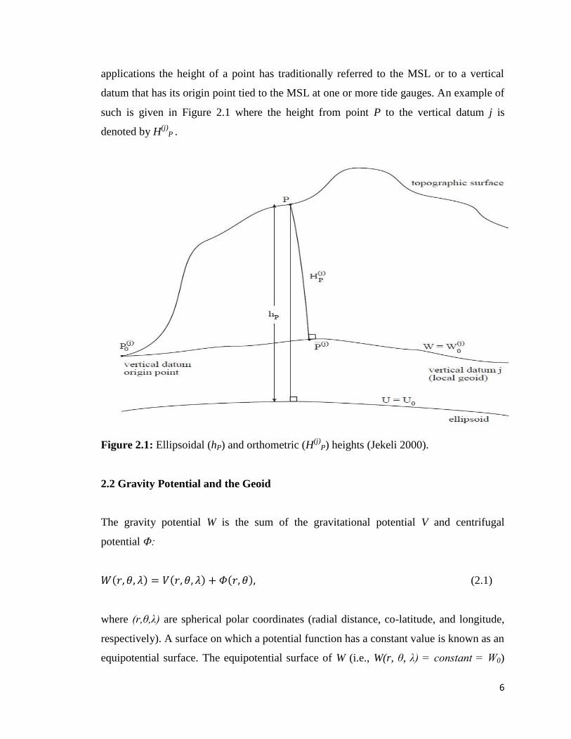
applications the height of a point has traditionally referred to the MSL or to a vertical
datum that has its origin point tied to the MSL at one or more tide gauges. An example of
such is given in Figure 2.1 where the height from point P to the vertical datum j is
denoted by H(j)
P .
Figure 2.1: Ellipsoidal (hP) and orthometric (H(j)
P) heights (Jekeli 2000).
2.2 Gravity Potential and the Geoid
The gravity potential W is the sum of the gravitational potential V and centrifugal
potential Φ:
(2.1)
where (r,θ,λ) are spherical polar coordinates (radial distance, co-latitude, and longitude,
respectively). A surface on which a potential function has a constant value is known as an
equipotential surface. The equipotential surface of W (i.e., W(r, θ, λ) constant W0)

7
that best agrees with the global MSL at rest is known as the geoid (Gauss 1828; Listing
1873). Today it is understood that the geoid surface will vary with time due to mass
deformations and re-distributions within the Earth. The distance between the ellipsoid
and the geoid surface is known as the geoid undulation or geoid height. The
determination of this quantity will be discussed in Section 2.6. It should be noted that the
local geoid in Figure 2.1 is synonymous with the local vertical datum in a specific datum
zone, which has traditionally been constrained by the local MSL at one or more tide
gauges. Globally, the datum offsets between local vertical datums (LVDs) and a globally
consistent geoid model can reach up to 1-2 m (Gerlach and Rummel 2013).
Functions that satisfy the Laplace equation (i.e., Δf ) are called harmonic functions.
Harmonic functions are analytic (i.e., continuous with continuous derivatives of any
order) and can be expanded into a spherical harmonic series. The gravitational potential
(i.e., the geopotential generated by the masses of the Earth including the atmosphere) is a
harmonic function, meaning that ΔV outside the masses, or in other words when the
density ρ is equal to zero. Thus, the gravitational potential can be expressed most
conveniently in terms of spherical harmonic functions (Heiskanen and Moritz 1967;
Jekeli 2000):
∑
(
)
∑ [ ] , (2.2)
where G is the Newton’s gravitational constant and M is the Earth’s mass (including the
atmosphere), R is the mean Earth radius, n is the degree, m is the order, n and Sn are
fully normalized spherical harmonic coefficients for degree and order n and m, and n
are fully normalized Legendre functions. Equation (2.2) is the solution to a boundary
value problem for the potential and only holds if the point of computation is in free space.
The convergence to the true gravitational potential is guaranteed only for points outside a
sphere enclosing all masses. In practice Eq. (2.2) will be truncated to a maximum degree
nmax as it is impossible in practice to expand the series to infinity.
When m=n=0, Eq. (2.2) reduces to:
8
(2.3)
Thus, the zero-degree term is simply the potential of a homogenous sphere and the higher
degree terms express the deviations from the potential of such a sphere.
On the other hand, the centrifugal potential is not a harmonic function. The Laplace
equation for the centrifugal potential is not zero (i.e., ΔΦ 2ω2). Due to this, the gravity
potential W is not a harmonic function either as it is a sum of the gravitational and
centrifugal potentials. In spherical coordinates the centrifugal potential can be written as
(Jekeli 2000):
(2.4)
where ωe is the Earth’s rotation rate. The gravity potential and its constituent potentials
(specifically the gravitational potential) are re-visited in Section 2.6 where geoid
modelling is discussed.
2.3 Height Systems
The relationship between the gravity vector and the gravity potential is:
(2.5)
where denotes the gradient operator. The gradient is a vector pointing in the direction
of the steepest descent of a function (i.e., perpendicular to its isometric lines). Therefore,
in the case of the gravity potential, the gradient of W is the vector perpendicular to the
equipotential surfaces. Thus, the relationship between the magnitude of the gravity vector
and the gravity potential may be written as:
9
| |
(2.6)
where dn is the differential path along the perpendicular. The minus sign indicates that
potential decreases with altitude, the path length is positive upwards, and the gravity
magnitude is positive. From equation (2.6) it follows that a height, which can be defined
as the distance along the plumb line (i.e., the curved line that intersect normally the
equipotential surfaces and to which the gravity vector is tangent) from a point P on the
surface of the Earth to the geoid (W0), is dependent on the gravity potential and the
gravity vector:
∫
(2.7)
where Hp is the height at point P with respect to the geoid W0 and Wp is the gravity
potential at point P.
There are three types of physical heights: dynamic heights, orthometric heights, and
normal heights. Each depends on the difference in gravity potential between the local
geoid and the point in question The local geoid can also define a local vertical datum
where a single point P(j)
0, which is assumed to the on the geoid and is accessible, through
for example a tide gauge, defines the vertical datum origin point (see Section 2.4).
The difference in the gravity potential between the local geoid and the point P is known
as the geopotential number:
(2.8)
where W ( )
is the potential of the local geoid, and WP is the gravity potential at point P.
Any point on the Earth’s surface has a unique geopotential number. If the geopotential
number is appropriately scaled (see Eq. (2.7)) it may be used as the height coordinate of
the point in question.
10
2.3.1 Dynamic Heights
The dynamic height of a point P is given by the equation:
(2.9)
where γ45 is the nominal value of normal gravity generally chosen at mid-latitude (e.g., at
45˚ latitude). Although dynamic heights are physically meaningful, they have no
geometric meaning—it is simply the potential in distance units relative to the geoid, as
the same constant scale factor is used for all dynamic heights within a particular datum.
2.3.2 Orthometric Heights
In contrast to dynamic heights, orthometric heights of a point P have a very definite
geometric interpretation: it is the distance above the local geoid along the plumb line,
which is curved due to the fact that equipotential surfaces are not parallel to each other.
The orthometric height is given by the following mathematical relationship:
(2.10)
where g ( )is the average value of gravity along the plumb line:
∫
(2.11)
where dH is a differential element along the plumb line and ( )
is at the base of the
plumb line on the local geoid. The ( )
term from Eq. (2.10) can be estimated from
measurements using the following relationship:
11
∫
(2.12)
However, the value of g ( ) cannot be evaluated exactly as this requires complete
knowledge of the mass density of the Earth’s crust. Thus, orthometric heights cannot be
exactly determined. The computation of orthometric height therefore depends on a
density hypothesis for the crust. For this purpose, a frequently utilized model assumes a
constant crustal density and constant topographic height in the region near the point P.
With this assumption, the average gravity along the plumb line between ( )
and P can be
obtained using a Prey reduction (Heiskanen and Moritz 1967):
[ (
)] (2.13)
The Prey reduction models the gravity value inside the crust by removing the attraction of
a Bouger plate (i.e., 2π ρ
) of constant density, which is followed by applying a free-
air downward continuation using the normal gravity gradient (i.e., dγ/dh), and lastly the
Bouger plate is restored. Using nominal values for the density and the gradient (i.e., 2670
kg/m3 and -0.0848 mgal/m) Eq. (2.13) simplifies to:
(
)
(2.14)
When substituting g r ( ) for g
( ) in Eq. (2.10), the orthometric height is known as
Helmert orthometric height. It can be determined with the combination of Eq. (2.10) and
Eq. (2.13) (Jekeli 2000):
( (
)
(
) (
)
) (2.15)
where the higher order terms contribute less than 10-10
.

12
Heiskanen and Mortiz (1967) assess that an error in the topographic mass density ρ of
approximately 600 kg/m3 at an elevation of approximately 1000 m will affect the
orthometric height by 25 mm, while Strange (1982) estimates this error to be up to 30
mm for elevations greater than 2000m. The topographic density of 600 kg/m3 represents
the largest range in mass-density that should be encountered in practice according to
Heiskanen and Mortiz (1967), but the changes in the mass-density may reach up to 1000
kg/m3.
2.3.3 Normal Heights
In order to avoid making a density hypothesis for the Earth’s crust, a geometrically
interpretable height may be estimated using an approximation of the gravity field that can
be calculated exactly at any given point. The approximation of the gravity field refers to
the normal gravity field, where the gravity field is generated by an Earth-fitting ellipsoid
that contains the total mass of the Earth, rotates with the Earth around its minor axis, and
is itself an equipotential surface of the gravity field it generates. The normal gravitational
field generated by the ellipsoid, Ve, can also be expressed by Eq. (2.2), though it will only
contain even zonal harmonics (i.e., m=0; no dependence on longitude since cos λ ) due
to the imposed symmetries of the ellipsoid (Jekeli 2000). Likewise, the normal
centrifugal potential can be determined using Eq. (2.4). Thus, the normal gravity potential
U can be defined as:
(2.16)
The normal gravity potential U can be evaluated anywhere in space on and above the
ellipsoid using four constants that define the size, shape, mass and rotation of the
ellipsoid. U is constant on the ellipsoid (i.e., U0) and can be calculated using the Pizzetti
formula (Heiskanen and Mortiz 1967):
√ √
(2.17)
13
where a and b are respectively the semi-major and semi-minor axis of the ellipsoid.
Similarly to the relationship between gravity and the gravity potential, the normal gravity
vector can be derived using
(2.18)
where the magnitude of can be calculated exactly anywhere on the ellipsoid using the
Somigliana-Pizzetti formula (Heiskanen and Mortiz 1967):
√ (2.19)
where γa and γb are the normal gravity at the equator and the pole respectively, and are
normally given as published values. The normal gravity can also be obtained above the
surface of the ellipsoid by the Taylor series expansion of γ, where the final expression up
to the 2nd
term is given by:
[
(
(
) )
] (2.20)
where h is the height above the surface of the ellipsoid and φ is the geodetic latitude.
The normal plumb line through a point P is the line that is perpendicular to equipotential
surfaces of the normal gravity field. On this plumb line, there is a point Q where the
normal gravity potential equals the actual gravity potential at point P (see Figure 2.2). In
other words, UQ is equivalent to WP. Thus, the normal geopotential number of Q is
defined as (Jekeli 2000):
(
) (2.21)
where WP has been replaced by the relationship given in Eq. (2.8).
14
Similarly to Eq. (2.12) from the previous section on orthometric heights, it follows that
∫
(2.22)
where is the point on the ellipsoid of the normal plumb line (see Figure 2.2), and d
denotes the differential path element along the normal plumb line. By dividing and
multiplying the right hand size of Eq. (2.22) by the length of the normal plumb line from
the ellipsoid to point Q (i.e., H*
Q in Figure 2.2) one obtains (Jekeli 2000):
(
)
(2.23)
where
∫
(2.24)
is the mean value of the normal gravity along the normal plumb line.
From Figure 2.2, it can be seen that the point Q lies on the telluroid. The telluroid is the
surface whose normal potential is equal to the actual gravity potential at the Earth’s
surface along the ellipsoidal normal. It should be noted that the telluroid is not an
equipotential surface. The distance between the telluroid and the Earth’s surface is known
as the height anomaly at P, ζP. The quasi-geoid is the surface defined by the separation ζP
from the ellipsoid.
15
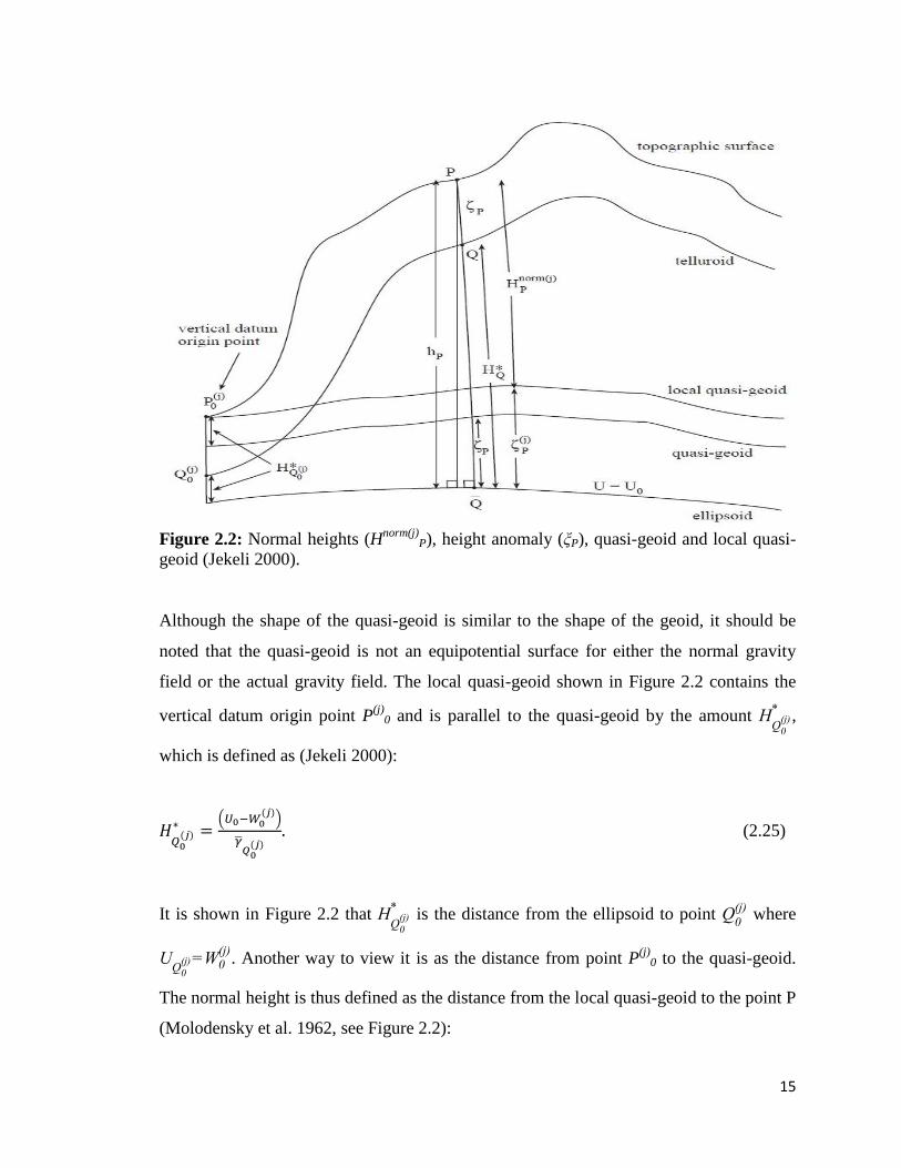
Figure 2.2: Normal heights (H
norm(j)P), height anomaly (ξP), quasi-geoid and local quasi-
geoid (Jekeli 2000).
Although the shape of the quasi-geoid is similar to the shape of the geoid, it should be
noted that the quasi-geoid is not an equipotential surface for either the normal gravity
field or the actual gravity field. The local quasi-geoid shown in Figure 2.2 contains the
vertical datum origin point P(j)
0 and is parallel to the quasi-geoid by the amount
( )
,
which is defined as (Jekeli 2000):
(
)
(2.25)
It is shown in Figure 2.2 that
( )
is the distance from the ellipsoid to point
( ) where
( ) W ( )
. Another way to view it is as the distance from point P(j)
0 to the quasi-geoid.
The normal height is thus defined as the distance from the local quasi-geoid to the point P
(Molodensky et al. 1962, see Figure 2.2):
16
. (2.26)
The average normal gravity γ
can be approximated from the expression (Heiskanen and
Mortiz 1967):
[ (
(
) )
(
)
]. (2.27)
Substituting Eq. (2.27) into Eq. (2.26) yields (Jekeli 2000):
[ (
(
) )
(
)
]. (2.28)
Lastly, the local height anomaly, which is the separation of the local quasi-geoid from the
ellipsoid, can be determined from the following relationship (Jekeli 2000, see Figure 2.2):
(
)
(2.29)
2.4 Definition and Realization of Classical Levelling Based Vertical Datums
A vertical reference system is defined as a system for elevations that supports physical
and geometric heights globally with a relative accuracy better than 10-9
(Ihde and
Sánchez 2005). A vertical reference frame is a realization of the vertical reference system
by a set of physical points or stations with precisely determined geopotential numbers
and geocentric coordinates referred to the Conventional Terrestrial Reference System
(CVRS Conventions 2007). Hence, the vertical datum has been defined as an
equipotential surface with a conventional value of W0 of Earth’s gravity potential.
Heights are defined with respect to this surface, or alternatively as a “coordinate surface
17
to which heights, taken as vertical coordinates, are referred” (Vaníček 1991). According
to Vaníček (1991), there are three kinds of vertical datums that are used in geodesy: the
geoid, the quasi-geoid, and the reference ellipsoid.
Torge (1980) defines the geoid as a surface of constant gravity potential W0 having been
reduced for the gravitational effects of luni-solar and atmospheric masses, and short
periodic variations in the Earth’s gravity field that coincides with the MSL after the effect
of sea surface topography over the oceans is removed, or more compactly, a level surface
where W=W0 that best approximates the MSL at rest. Due to the existence of long term
gravity field variations, the geoid is generally referred to a specific time epoch (Heck and
Rummel 1989).
Vaníček (1991) presents two practical options for identifying the desired equipotential
surface where W=W0. First is the abstract option, where one specifies a constant value of
the Earth’s gravity potential W=W0=const, which defines the geoid as one specific level
surface. The second option is known as the geometrical option, and it requires that the
chosen horizontal surface approximates in a specific way the MSL surface.
Traditionally, height systems have been defined by the long-term averages of one or
many local reference benchmarks, for example by averaging the sea level observations to
obtain MSL constrained to one or several tide gauges, with the assumption that the MSL
coincides with the geoid. However, phenomena due to tides, sea surface topography,
currents, and storm surges cause the MSL to deviate from an equipotential surface; thus
the discrepancy between the MSL and the geoid can reach up to 2 m (Balasubramania
1994). Moreover, the relationship between the observed MSL and land benchmarks is not
constant due to changes in sea level and the uplift/subsidence of land, causing datums at
different epochs to refer to different reference levels. This effect of defining the vertical
datum in relation to a local MSL is responsible for the vertical datum offset between
different regional and national datums. Most countries have been using regional vertical
datums as local reference systems, and it is estimated that more than one hundred
18
regional vertical datums have been derived all over the world (Balasubramania 1994; Pan
and Sjöberg 1998).
Thus, the realization of a vertical datum has generally been accomplished by locating a
point of zero height, which is generally located by obtaining the averaged long term MSL
at a tide gauge station, which is linked to a reference benchmark either a short distance
away from the tide gauge or located directly on the tide gauge. This benchmark is
assigned as the starting point of the levelling network and defines the zero height value of
the vertical datum (Vaníček 1991). Orthometric, dynamic, and normal heights can then
be determined by adding gravity dependent corrections to the leveled height increments
(Rummel and Teunissen 1988). This is what will be referred to as a “classical levelling
based vertical datum”. Five main approaches for defining a regional vertical datum are
described below (Vaníček 1991; Ihde 2007; CVRS Conventions 2007):
1) The geoid surface is defined by the MSL measurements obtained from the tide
gauge network on the coasts of the country. The datum is fixed to zero at these
stations. Due to the discrepancy between the MSLs at the selected tide gauge
stations and the geoid, distorted heights will result from this approach. It is
assumed that the tide gauge records do not include any errors or that the error
level is acceptable when fixing the datum to zero at the defined tide gauge
network.
2) The vertical datum is defined by performing a free-network adjustment where
only one tide gauge or point is held fixed. The heights from the adjustment are
shifted so that the mean height of all tide gauges equals zero. This approach is
similar to (1) with the exception that the MSL observations made at other tide
gauges are not included, and thus the MSL is defined from the records of a single
tide gauge only.
3) The mean sea surface topography (MSST) values at tide gauge stations are
estimated from satellite altimetry and hydrostatic models. Satellite altimetry
19
measures sea surface heights (SSHs), which is the height of the water surface
given with respect to a reference ellipsoid. One can obtain the MSST or the mean
dynamic topography (MDT) using a geoid model and altimetry derived SSH
values, as the SSH values are generally averaged over time. SST, MSST and
MDT are used synonymously in this thesis and refer the height of the mean sea
surface above the geoid. The network is adjusted by forcing MSL-MSST to zero
for all tide gauge stations. With this method of realizing a regional vertical datum,
most of the drawbacks for method (1) and (2) are eliminated, though it should be
noted that satellite altimetry has poor performance in coastal regions where tide
gauges are located due to contamination of the altimetry footprint by land.
Moreover, in shallow regions, global ocean circulation models derived from
altimetry and hydrostatic models may have up to a decimeter level uncertainty
(Shum et al. 1997).
4) The vertical datum is defined in the same way as in method (3) with the exception
that the reference tide gauges are allowed to float in the adjustment by error
estimates. In this approach all MSL and SST information at the reference tide
gauges can be incorporated.
5) Lastly, the vertical datum is defined as in method (4) with the exception that
orthometric heights are estimated from satellite-based ellipsoidal heights and
gravimetric geoid heights. As the satellite-derived heights are referenced to a
global reference ellipsoid, the regional datum is linked to a global vertical
reference surface. This approach may be used to realize an international world
height system or a global vertical datum (Colombo 1980; Balasubramania 1994).
The link between the traditional levelling based vertical datum and the geoid is realized
by GNSS positioning at the benchmarks of the vertical control network. Theoretically it
is expected that hP-H(j)
P-NP=0, where hP is the ellipsoidal height, H(j)
P is the orthometric
height, and NP is the geoid undulation. However, in practice it does not equal zero due to
various inconsistencies of the geoid and ellipsoidal heights, systematic errors in the
20
levelling network, limitations in the measurement accuracy of the vertical component by
GNSS, biases present in gravity anomalies, long wavelength geoid errors, and
geodynamic phenomena (Rangelova 2007; Kotsakis and Sideris 1999).
2.5 Classical Levelling Based Vertical Datums in North America
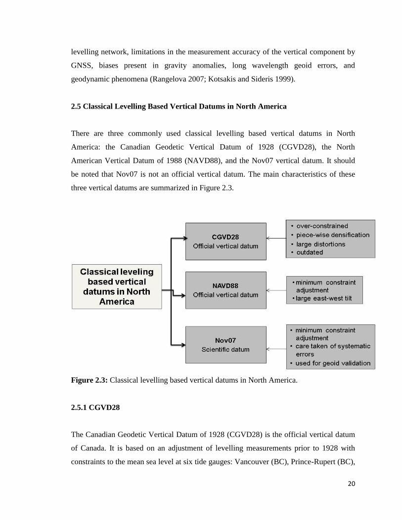
There are three commonly used classical levelling based vertical datums in North
America: the Canadian Geodetic Vertical Datum of 1928 (CGVD28), the North
American Vertical Datum of 1988 (NAVD88), and the Nov07 vertical datum. It should
be noted that Nov07 is not an official vertical datum. The main characteristics of these
three vertical datums are summarized in Figure 2.3.
Figure 2.3: Classical levelling based vertical datums in North America.
2.5.1 CGVD28
The Canadian Geodetic Vertical Datum of 1928 (CGVD28) is the official vertical datum
of Canada. It is based on an adjustment of levelling measurements prior to 1928 with
constraints to the mean sea level at six tide gauges: Vancouver (BC), Prince-Rupert (BC),

21
Point-au-Père (QC), Halifax (NS), Yarmouth (NS), and New York City and is accessible
through approximately 80,000 benchmarks mostly distributed in southern Canada
(Véronneau 2006). All levelling measurements consisting of re-observations or
extensions since the original adjustment have been processed according to the same
procedure and constrained to the 1928 original adjustment. The CGVD28 heights are said
to be “normal-orthometric heights” given that the heights are evaluated using normal
gravity values based on latitude instead of actual gravity measurements. Hence, the
heights are neither orthometric nor normal heights and as a result CGVD28 does not
coincide with either the geoid or the quasi-geoid (Véronneau 2006). Moreover, the sea
surface topography at the tide gauge stations, the rising of the sea level due to melting of
glaciers and thermal expansion, earthquakes, frost heave, local instabilities, and the fact
that land elevation is changing due to the rebound/subsidence of the Earth’s crust (i.e.,
post-glacial rebound) have not been accounted for in the realization of the CGVD28.
Additionally, the levelling data used in CGVD28 are not corrected for systematic errors
due to atmospheric refraction, rod calibration, rod temperature, and the effects of solar
and lunar tides on the Earth’s geopotential surfaces. The CGVD28 datum has a national
distortion that ranges from -65 cm in Eastern Canada to 35 cm in Western Canada with
respect to an equipotential surface due to various correction omissions, approximations,
and the fact that the vertical control network was established over time in a piece-wise
manner (Véronneau and Héroux 2006). Currently, the network is characterized by a rapid
rate of degradation due to destruction and loss of physical markers and limited
maintenance as Canada is planning to implement a geoid-based GNSS-accessible vertical
datum by 2013 (Véronneau et al. 2006).
2.5.2 NAVD88
The North American Vertical Datum of 1988 (NAVD88) was the result of a joint effort
in the 1970s and 1980s by the governmental agencies of U.S.A., Canada, and Mexico to
unify the vertical control networks on the continent. It is currently the official vertical
datum in the U.S.A. The NAVD88 was established by the minimum-constraint
adjustment of geodetic levelling observations in Canada, U.S.A., and Mexico, holding
22
fixed the height of the primary tidal benchmark at Rimouski, Quebec, Canada. Due to the
demonstrated spatial (and to a lesser extent temporal) variations in the sea surface
topography, additional tidal benchmark elevations were not utilized. NAVD88 heights
are Helmert orthometric heights. The NAVD88 datum contains a large east-west tilt of
1.5 m from the Atlantic to Pacific coasts, possibly due to the accumulation of systematic
errors in the levelling network, and as a result was never officially adopted in Canada
(Véronneau and Héroux 2006).
2.5.3 Nov07
The Nov07 vertical datum is the latest realization of a series of minimum-constraint
adjustments of the federal first-order levelling network in Canada. However, it should be
noted that Nov07 is not an official vertical datum. It has been realized for the purpose of
validating geoid models in North America with the heights of benchmarks given as
Helmert orthometric heights. The main network covers the continental main land, and
includes independent networks for Newfoundland, Vancouver Island, and various other
islands. In addition, there is a series of independent local networks around tide gauges in
the northern region of Canada. The former tide gauge in Pointe-au-Père, Quebec (QC), on
the lower St. Lawrence River, is the fixed station for the Canadian mainland network.
Similarly, each of the other sub-regions, containing their own independent networks,
have their adjustments tied to their own respective fixed tide gauge stations. It was found
that the best approach to decrease the systematic error for Nov07 was to adjust together
only the most recent levelling measurements that allow a continuous network between
Vancouver and Halifax. This resulted in a discrepancy between the two coasts of 80 cm,
which represents about 20 to 30 cm of systematic error over approximately 6000 km of
levelling lines (Véronneau 2012). The remaining 50-60 cm accounts for the separation
between the mean water levels on the west and east coasts of Canada (Véronneau 2012).
This separation was first reported by Sturges (1967), where it was shown that MSL
values at tide gauges on the Pacific coast appeared to be systematically 60-70 cm higher
than those of similar latitude on the Atlantic coast, which was later shown to be caused
by a combination of ocean density differences and boundary current effects (Sturges
1974).

23
2.5.4 Problems Presented by Classical Levelling Based Vertical Datums and the
Adoption of a Geoid-Based and GNSS-Accessible Vertical Datum
In the discussion of the vertical datums CGVD28, NAVD88, and Nov07 it is evident that
classical levelling based vertical datums have many problems. Firstly, maintaining and
realizing a vertical datum based on spirit levelling is expensive, time consuming, and
laborious. Moreover, it provides limited coverage over a geographic region, and is
especially difficult to do in remote areas and mountainous terrain. Other problems relate
to maintaining the vertical control network over time, as benchmark become unstable or
disappear completely, and there are temporal effects such as post-glacial rebound that
also need to be taken into account. Of course, there is the problem of existing systematic
levelling errors and distortions found within the vertical control network. Moreover, as
the MSL varies both spatially and temporally, regional vertical datums will refer to
different reference surfaces. Currently, there are hundreds of classical levelling based
vertical datums in the world and as each of these datums refer to their own reference
surface defined by a local MSL, there is a need to be able to relate these datum to each
other, or in other words, to unify these datums. This is especially important for
engineering projects between two neighbouring countries, or even for a country that may
have two different datum zones (e.g., island vs. mainland regions).
Due to the various issues presented by classical levelling based vertical datums, the
Geodetic Survey Division (GSD) of Natural Resources Canada (NRCan) and the U.S.A.
National Geodetic Survey (NGS) have decided to modernize the way vertical datums are
realized by implementing a geoid-based and GNSS-accessible vertical datum. Adopting a
geoid-based vertical datum means that there will be no more need for expensive and
time-consuming spirit levelling in order to establish a vertical control network. The issue
of benchmark stability and coverage is also resolved. The geoid is also a fairly stable
reference surface that only has to be updated, in the North American context specifically,
for temporal effects such as post glacial rebound once every ten years (Rangelova 2007).
Moreover, a geoid-based vertical datum is compatible with space-based positioning
techniques such as GNSS. This concept is illustrated by Figure 2.4. The geoid surface is
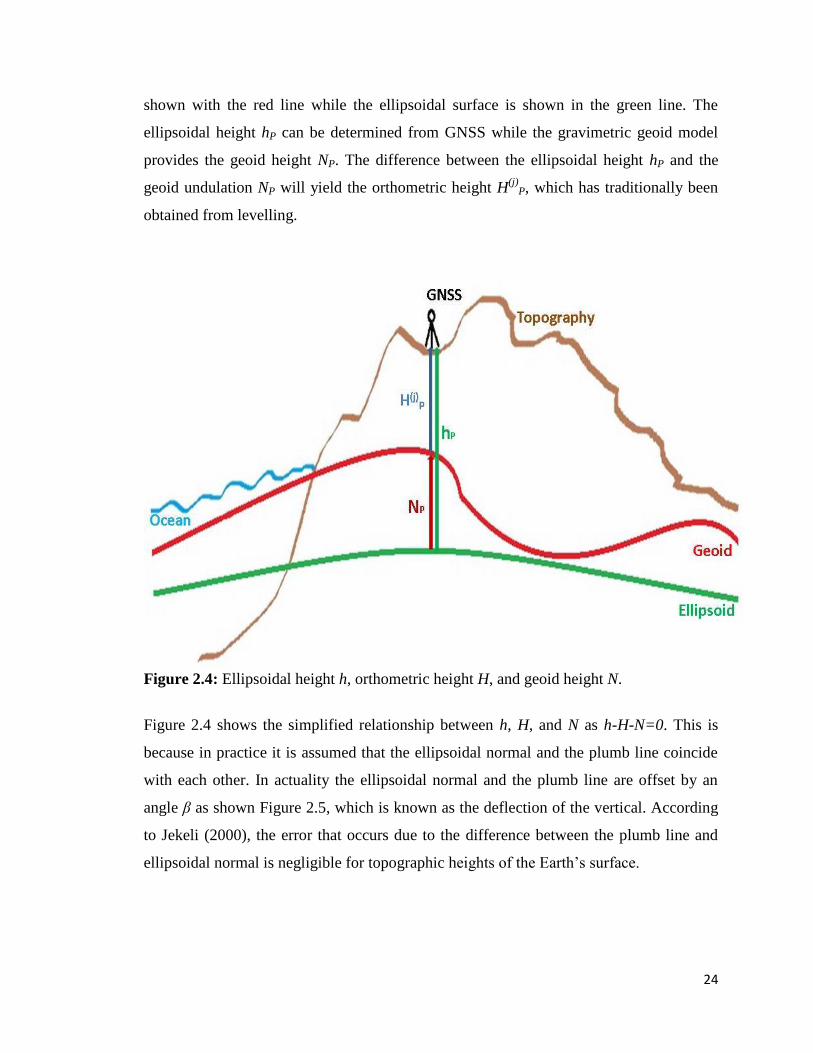
24
shown with the red line while the ellipsoidal surface is shown in the green line. The
ellipsoidal height hP can be determined from GNSS while the gravimetric geoid model
provides the geoid height NP. The difference between the ellipsoidal height hP and the
geoid undulation NP will yield the orthometric height H(j)
P, which has traditionally been
obtained from levelling.
Figure 2.4: Ellipsoidal height h, orthometric height H, and geoid height N.
Figure 2.4 shows the simplified relationship between h, H, and N as h-H-N=0. This is
because in practice it is assumed that the ellipsoidal normal and the plumb line coincide
with each other. In actuality the ellipsoidal normal and the plumb line are offset by an
angle β as shown Figure 2.5, which is known as the deflection of the vertical. According
to Jekeli (2000), the error that occurs due to the difference between the plumb line and
ellipsoidal normal is negligible for topographic heights of the Earth’s surface.
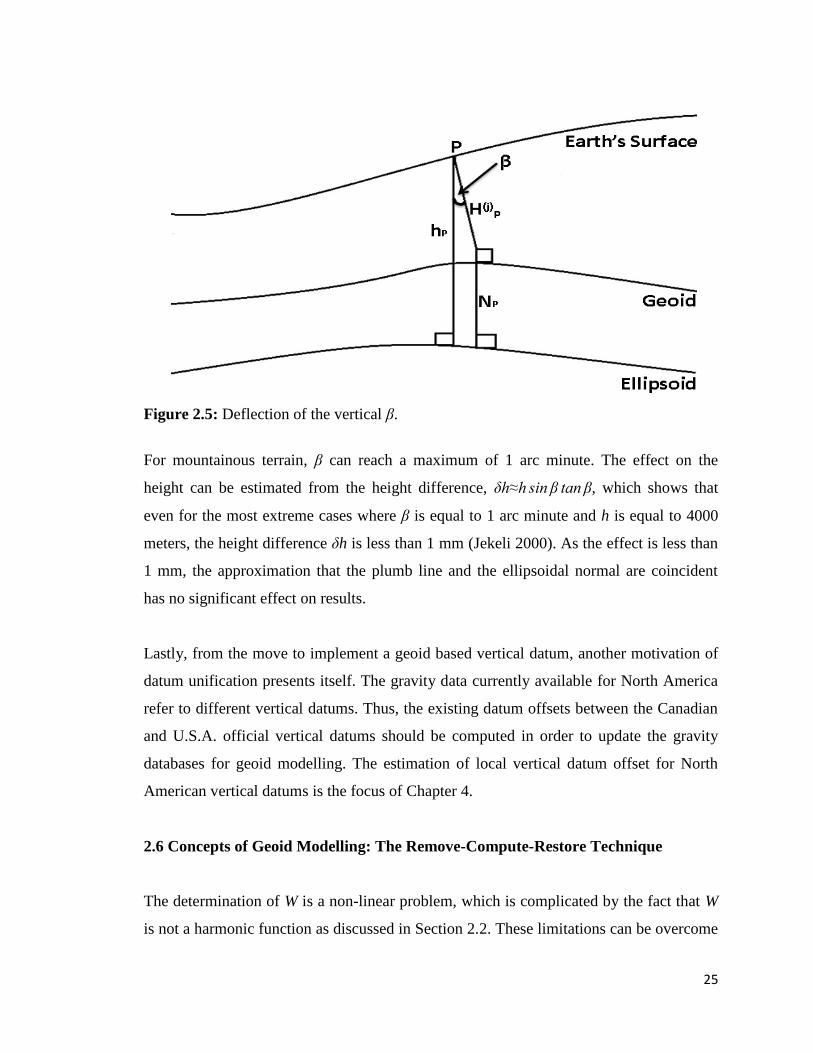
25
Figure 2.5: Deflection of the vertical β.
For mountainous terrain, β can reach a maximum of 1 arc minute. The effect on the
height can be estimated from the height difference, δh h s n β tan β, which shows that
even for the most extreme cases where β is equal to 1 arc minute and h is equal to 4000
meters, the height difference δh is less than 1 mm (Jekeli 2000). As the effect is less than
1 mm, the approximation that the plumb line and the ellipsoidal normal are coincident
has no significant effect on results.
Lastly, from the move to implement a geoid based vertical datum, another motivation of
datum unification presents itself. The gravity data currently available for North America
refer to different vertical datums. Thus, the existing datum offsets between the Canadian
and U.S.A. official vertical datums should be computed in order to update the gravity
databases for geoid modelling. The estimation of local vertical datum offset for North
American vertical datums is the focus of Chapter 4.
2.6 Concepts of Geoid Modelling: The Remove-Compute-Restore Technique
The determination of W is a non-linear problem, which is complicated by the fact that W
is not a harmonic function as discussed in Section 2.2. These limitations can be overcome
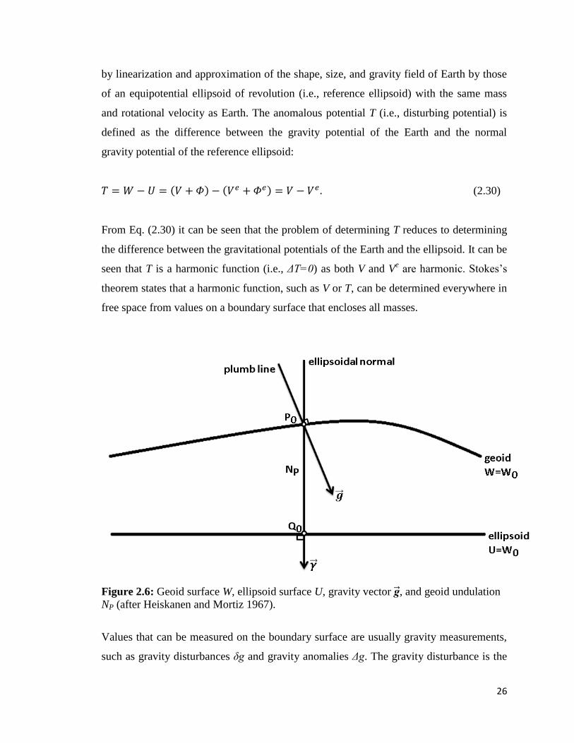
26
by linearization and approximation of the shape, size, and gravity field of Earth by those
of an equipotential ellipsoid of revolution (i.e., reference ellipsoid) with the same mass
and rotational velocity as Earth. The anomalous potential T (i.e., disturbing potential) is
defined as the difference between the gravity potential of the Earth and the normal
gravity potential of the reference ellipsoid:
(2.30)
From Eq. (2.30) it can be seen that the problem of determining T reduces to determining
the difference between the gravitational potentials of the Earth and the ellipsoid. It can be
seen that T is a harmonic function (i.e., ΔT ) as both V and Ve are harmonic. Stokes’s
theorem states that a harmonic function, such as V or T, can be determined everywhere in
free space from values on a boundary surface that encloses all masses.
Figure 2.6: Geoid surface W, ellipsoid surface U, gravity vector , and geoid undulation
NP (after Heiskanen and Mortiz 1967).
Values that can be measured on the boundary surface are usually gravity measurements,
such as gravity disturbances δg and gravity anomalies Δg. The gravity disturbance is the
27
difference between the gravity the normal gravity at the same point. A gravity anomaly is
the difference between the value of gravity at a point P0 on the geoid and the value of the
normal gravity at a point Q0 on the ellipsoid, which corresponds with the point P0 on the
geoid surface (see Figure 2.6).
The fundamental equation of physical geodesy is an important equation that relates
gravity anomalies to the disturbing potential T (Heiskanen and Mortiz 1967):
(2.31)
Equation (2.31) only holds on the geoid surface and is the boundary condition in Stokes’s
Boundary Value Problem (BVP). In Stokes’s problem the boundary surface is the geoid
with potential W, approximated by the ellipsoid with potential U. The surface of the geoid
is given by geoid undulations or geoid heights, N, which depends on the disturbing
potential through Bruns’s equation (Heiskanen and Mortiz 1967):
, (2.32)
and by selecting =
= W0 = const., the equation simplifies to:
(2.33)
Thus, Bruns’s formula shows that the surface of the geoid can be determined provided
that T is known. Equation (2.31) shows that T can be estimated from gravity observations
on the boundary surface. As the boundary surface in Stokes’s BVP is the geoid, the
gravity measurements need to the reduced to the geoid by terrain reductions, which
requires assumptions about the topographic density distribution.

28
Stokes’s BVP is based on the mathematical definition given by the Laplace differential
equation:
(2.34)
with the boundary condition given in spherical approximation (Heiskanen and Mortiz
1967) as:
. (2.35)
It should be noted that spherical approximation is used only in equations relating the
small quantities of anomalous potential T, geoid undulations N, gravity anomalies Δg, and
deflections of the vertical, among others. The reference is not the sphere but the ellipsoid,
thus the normal gravity γ in Δg and δg must be computed precisely for the ellipsoid.
Analytical solutions to the Stokes’s BVP can be expressed as spherical harmonic series
since T is harmonic. Thus, using Bruns’s equation the geoid undulation can also be
expressed in terms of spherical harmonic series (in a spherical approximation on the
geoid):
∑ ∑ [ ]
, (2.36)
where n and Sn are fully normalized geopotential coefficients of the anomalous
potential, n are the fully normalized Legendre functions (Heiskanen and Moritz 1967),
and φ , λ are the latitude and longitude of the computational point. Similarly, using Eq.
(2.35), Δg can also be expressed in terms of spherical harmonic series:
∑ ∑ [ ]
, (2.37)
where γ is the mean normal gravity.
29
As well, the analytical solution of Stokes’s BVP can be expressed by the Stokes integral
(Heiskanen and Moritz 1967):
∬
(2.38)
where σ denotes the Earth’s surface. S ψ is the Stokes’ kernel function given by
(Heiskanen and Moritz 1967):
(
) (2.39)
In Eq. (2.39), ψ is the spherical distance between the data point (φ, λ) and the
computation point (φP, λP):
(2.40)
The geoid signal can be decomposed into long, medium, and short wavelength
components as shown in Figures 2.7 and 2.8. The long wavelength components of the
geoid signal come from the harmonic coefficients of global geopotential models (GGMs;
this is also synonymous with global gravity models), which are derived primarily from
data collected from dedicated satellite gravity field missions. The medium wavelength
components are a result of local gravity anomalies, which can be observed from
terrestrial, shipborne, airborne, and even satellite platforms. The short wavelength or high
frequency components of the gravity field signal or the geoid signal are mainly a result of
the Earth’s topography. This information is usually available from digital elevation
models (DEMs).
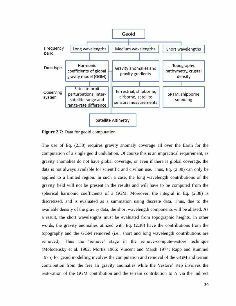
30
Figure 2.7: Data for geoid computation.
The use of Eq. (2.38) requires gravity anomaly coverage all over the Earth for the
computation of a single geoid undulation. Of course this is an impractical requirement, as
gravity anomalies do not have global coverage, or even if there is global coverage, the
data is not always available for scientific and civilian use. Thus, Eq. (2.38) can only be
applied to a limited region. In such a case, the long wavelength contributions of the
gravity field will not be present in the results and will have to be computed from the
spherical harmonic coefficients of a GGM. Moreover, the integral in Eq. (2.38) is
discretized, and is evaluated as a summation using discrete data. Thus, due to the
available density of the gravity data, the short wavelength components will be aliased. As
a result, the short wavelengths must be evaluated from topographic heights. In other
words, the gravity anomalies utilized with Eq. (2.38) have the contributions from the
topography and the GGM removed (i.e., short and long wavelength contributions are
removed). Thus the ‘remove’ stage in the remove-compute-restore technique
(Molodensky et al. 1962; Mortiz 1966; Vincent and Marsh 1974; Rapp and Rummel
1975) for geoid modelling involves the computation and removal of the GGM and terrain
contribution from the free air gravity anomalies while the ‘restore’ step involves the
restoration of the GGM contribution and the terrain contribution to N via the indirect
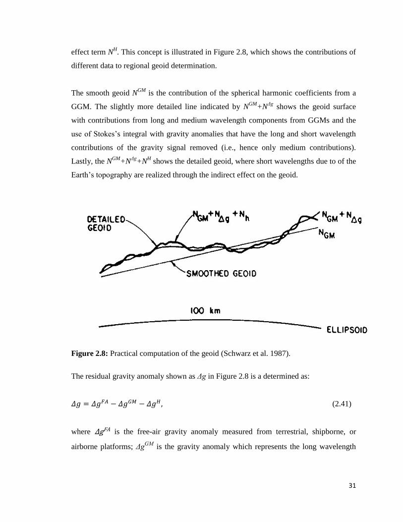
31
effect term NH. This concept is illustrated in Figure 2.8, which shows the contributions of
different data to regional geoid determination.
The smooth geoid NGM
is the contribution of the spherical harmonic coefficients from a
GGM. The slightly more detailed line indicated by NGM
+NΔg
shows the geoid surface
with contributions from long and medium wavelength components from GGMs and the
use of Stokes’s integral with gravity anomalies that have the long and short wavelength
contributions of the gravity signal removed (i.e., hence only medium contributions).
Lastly, the NGM
+NΔg
+NH shows the detailed geoid, where short wavelengths due to of the
Earth’s topography are realized through the indirect effect on the geoid.
Figure 2.8: Practical computation of the geoid (Schwarz et al. 1987).
The residual gravity anomaly shown as Δg in Figure 2.8 is a determined as:
(2.41)
where is the free-air gravity anomaly measured from terrestrial, shipborne, or
airborne platforms; Δg
is the gravity anomaly which represents the long wavelength
32
component of the gravity signal and is determined from a finite global geopotential
model; and lastly, Δg
is the topography-reduced gravity anomaly.
To summarize, NGM
and ΔgGM
can be evaluated using Eq. (2.36) and (2.37). For small
distances, inside a certain area E, one may use the planar approximation for Eq. (2.38)
where the first term in the S(ψ) is the dominant one (Sansó and Sideris 2013):
, (2.42)
(2.43)
and therefore Eq. (2.38) simplifies to:
∬
(2.44)
where
√ (2.45)
The coordinates of the data points are denoted by (x, y) and the coordinates of the
computation points are denoted by (xp, yP).
It has already been mentioned that Eq. (2.38) only gives the geoid undulation provided
that no masses are outside the geoid surface. One way to take care of topographic masses
of density ρ is through Helmert’s 2nd
condensation reduction, which can be approximately
applied in three steps (see Figure 2.9; Sansó and Sideris 2013):
1) remove all masses above the geoid,
2) lower the stations from P to P0 using the free-air reduction F,
3) and restore masses condensed on a layer on the geoid with density σ ρ .
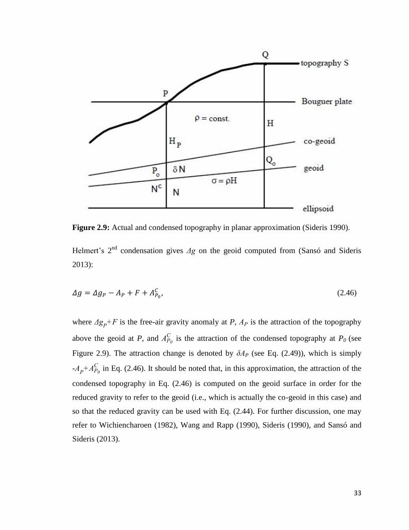
33
Figure 2.9: Actual and condensed topography in planar approximation (Sideris 1990).
Helmert’s 2nd
condensation gives Δg on the geoid computed from (Sansó and Sideris
2013):
, (2.46)
where Δg is the free-air gravity anomaly at P, is the attraction of the topography
above the geoid at P, and
is the attraction of the condensed topography at P0 (see
Figure 2.9). The attraction change is denoted by δ P (see Eq. (2.49)), which is simply
-
in Eq. (2.46). It should be noted that, in this approximation, the attraction of the
condensed topography in Eq. (2.46) is computed on the geoid surface in order for the
reduced gravity to refer to the geoid (i.e., which is actually the co-geoid in this case) and
so that the reduced gravity can be used with Eq. (2.44). For further discussion, one may
refer to Wichiencharoen (1982), Wang and Rapp (1990), Sideris (1990), and Sansó and
Sideris (2013).
34
Due to the shifting masses, the potential changes as well by an amount known as the
indirect effect on the potential (Sansó and Sideris 2013):
(2.47)
where T is the potential of the topographic masses at P0 and T is the potential of the
condensed masses at P0. Due to this potential change, Eq. (2.38) with Δg from Eq. (2.46)
produces a surface that in known as the co-geoid (i.e., a surface different from the geoid).
The difference between the geoid and the co-geoid is denoted by δN in Figure 2.9, which
is the indirect effect of the shifted topography on the geoid. Ideally, the indirect effect
should be small (i.e., the co-geoid should be near the geoid) in order to allow
approximations in the geoid modelling computations. Helmert reduced gravity anomalies
yields a small indirect effect (e.g., δN/ H 1m/3km; Sansó and Sideris 2013) and is
therefore very suitable for geoid determination. Before one can apply Eq. (2.38), the
gravity anomalies must be transformed from the geoid to the co-geoid by applying a
correction δΔg known as the indirect effect on gravity (Sansó and Sideris 2013):
(2.48)
The final geoid height is a sum of the co-geoid height and the indirect effect on the geoid.
When using the remove-compute-restore technique the terrain effect on Δg and the
indirect effect can be respectively approximated in planar approximation as (Sansó and
Sideris 2013):
∬
(2.49)
and
∬
(2.50)
35
Thus the remove-compute-restore technique can be applied as follows:
1) Earth surface gravity observations should be reduced on to the geoid.
2) Compute the long wavelength component of the gravity field signal, i.e., ΔgGM
and NGM
, using Eq. (2.36) and Eq. (2.37).
3) Compute the topography-reduced gravity anomaly using Eq. (2.49).
4) Compute the residual gravity anomaly using Eq. (2.41).
5) Evaluate the residual or co-geoid heights by applying Stokes’s integral (i.e., Eq.
(2.44)).
6) Compute the indirect effect of the topography on the geoid using Eq. (2.50).
7) Restore the effects of the long (i.e., geoid undulations determined from the GGM)
and short wavelength components (i.e., indirect effect on the geoid) of the geoid
signal to the residual/co-geoid heights (i.e., geoid heights from step (5)).
8) In the case that the reference ellipsoid mass Me and the normal gravity potential
U0 are different from that of the geoid add the zero-degree term to the geoid
undulations (Heisaknen and Mortiz 1967):
(2.51)
where Re is the mean radius of the reference ellipsoid.
On a final note, the use of Eq. (2.38) is computationally time consuming due to the fact
that the integration must take place over the entire surface of the Earth. This can be
overcome by reducing the size of the integration area by modifying the Stokes kernel
function, as the truncation error that results by limiting the area of integration of the
terrestrial gravity anomalies to a spherical cap can be reduced by an appropriate
modification of the Stokes kernel (Molodensky et al. 1962; Jekeli 1982; Hsu 1984).
Alternatively, increasing the size of the integration area has been shown to improve the
results (Schwarz 1984; Sjöberg 1986), though these methods have not proven to be
superior to the remove-compute-restore technique (Sansó and Sideris 2013). However,
integrals such the one shown in Eq. (2.44) are convolution integrals, and can thus be
36
evaluated by fast Fourier techniques (FFT) provided that the data is given on regular
grids (Sansó and Sideris 2013). Using FFT there is no need for time consuming point-
wise numerical summations. Moreover, FFT gives results on the same grid as the data
was provided on. Therefore, spectral techniques based on FTT overcome the problem of
slow computation speed and provide a homogenous coverage of results, which is
beneficial for interpolation and plotting purposes (Sansó and Sideris 2013). Moreover,
with FFT there is also no need to modify the Stokes kernel function (Schwarz et al. 1987;
Sideris and Forsberg 1990). It is thus recommended that for the computation of large
regional and continental geoids, spectral techniques such as FFT should be implemented,
especially since gravity and terrain data are readily available on regular grids (Sansó and
Sideris 2013).
Gravsoft (developed by C.C. Tscherning, R. Forsberg, P. Knudsen and D. Arabelos at the
University of Copenhagen) and FFTGeoid (developed by Y.C. Li and M.G. Sideris at the
University of Calgary) software products may be used for geoid modelling. It should be
noted that Gravsoft is not commercially available; however it can be made available by
request for the purpose of scientific research.
Lastly, as the focus of this thesis is not geoid modelling but rather the contribution of the
GOCE dedicated satellite gravity field mission to the application of vertical datum
unification and to the determination of W0, the treatment of geoid modelling has not been
exhaustive herein. For full derivations and more details on any of the material covered in
this chapter, Hofmann-Wellenhof and Moritz (2006), Heiskanen and Moritz (1967),
Jekeli (2000), and Sansó and Sideris (2013) should be consulted.

37
CHAPTER 3
EVALUATION OF GOCE GLOBAL GEOPOTENTIAL MODELS
3.1 Introduction
As discussed in the previous chapter, a global geopotential model or a global gravity
model is a set of coefficients that model the external gravity field of the Earth and are
derived from data collected from dedicated satellite gravity field missions and/or
terrestrial data. These coefficients are known as spherical harmonic coefficients and can
be used to compute different functionals of the Earth’s gravity field. The three dedicated
satellite gravity field missions are the Challenging Mini-Satellite Payload (CHAMP), the
Gravity Recovery and Climate Experiment (GRACE), and the GOCE mission. The
CHAMP satellite was launched July 15, 2000 with the objective to map the Earth’s
geopotential via the analysis of orbit perturbations (Reigber et al. 2002). The GRACE
mission was launched a few years later on March 17, 2002 with the objective to map the
global gravity field with a spatial resolution of 400 to 40,000 km every thirty days, and
has contributed significantly to the understanding of the time-variable aspect of the
Earth’s gravity field (Tapley et al. 2004). CHAMP and GRACE have provided static
gravity field solutions at the decimetre level of geoid accuracy up to degree and order 60
and 120, respectively (Sneeuw and Schaub 2004). Lastly, GOCE was launched on March
17, 2009 by the European Space Agency in order to measure the Earth’s gravity field at
an unprecedented accuracy and spatial resolution (Drinkwater et al. 2003). By the end of
its mission, the GOCE satellite is expected to determine gravity anomalies with an
accuracy of 1 mGal and the geoid with an accuracy of 1-2 cm while achieving a spatial
resolution of 100 km. In order to put the GOCE accuracy requirement into context, the
estimated cumulative geoid accuracy for the combined model EGM2008, which contains
terrestrial gravity data, is 7 cm at degree and order 200 while for the GRACE only
satellite model itg-grace2010s (Mayer-Gürr et al. 2010) it is 20 cm at degree and order
180 (Pail et al. 2011). Since the launch of the GOCE satellite, four generations of GOCE-
based GGMs have been released. These GGMs are available for download from the
International Centre for Global Earth Models (ICGEM, http://icgem.gfz-
38
potsdam.de/ICGEM/). Gruber et al. (2011) have shown that with two months of GOCE
data, the global geoid accuracy is about 5-6 cm with a 111 km spatial resolution. With the
recent release of fourth generation GOCE GGMs that contain approximately 27 months
of GOCE observations, the global geoid accuracy is approximately 1.2 cm at a spatial
resolution of 100 km, which corresponds to a degree and order of approximately 200 (see
Figure 3.9).
The performance of GGMs can be assessed using external datasets such as geoid heights
obtained from GNSS and levelling, astro-geodetic deflections, and gravity anomalies,
among others (see, e.g., Gruber 2004; Gruber 2009; Hirt et al. 2010; Hirt et al. 2011; Hirt
et al. 2012; Huang and Véronneau 2009; Kotsakis and Katsambalos 2009; Ince et al.
2012). External or independent datasets refer to quantities that have not been utilized in
the construction of the GGMs. The objective of this chapter is to evaluate the
performance of satellite-only GOCE-based GGMs in North America using geoid heights
obtained from GNSS and levelling in order to determine the best GOCE-based model in
North America for height system unification and W0 determination. The use of a GOCE
satellite-only GGM is preferred for such applications because it provides a globally
consistent and unbiased geoid (Gerlach and Rummel 2013). Thus, the aim is to show
which GOCE GGM performs best in Canada and the U.S.A.
In the next section of this chapter, the satellite gravity missions CHAMP, GRACE, and
GOCE are briefly reviewed. In Section 3.3, the methodology and distribution of the
GNSS/levelling benchmarks used for the evaluation of GOCE GGMs in North America
are described. Results are presented and discussed in Section 3.4 and a summary is given
in Section 3.5.
3.2 Overview of Dedicated Satellite Gravity Field Missions
According to Rummel et al. (2002), when designing dedicated satellite gravity field
missions the following four requirements should be considered:
1) uninterrupted satellite tracking in three spatial dimensions,
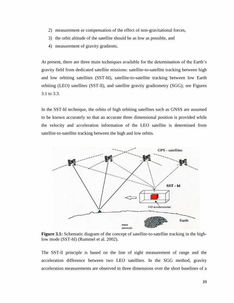
39
2) measurement or compensation of the effect of non-gravitational forces,
3) the orbit altitude of the satellite should be as low as possible, and
4) measurement of gravity gradients.
At present, there are three main techniques available for the determination of the Earth’s
gravity field from dedicated satellite missions: satellite-to-satellite tracking between high
and low orbiting satellites (SST-hl), satellite-to-satellite tracking between low Earth
orbiting (LEO) satellites (SST-ll), and satellite gravity gradiometry (SGG); see Figures
3.1 to 3.3.
In the SST-hl technique, the orbits of high orbiting satellites such as GNSS are assumed
to be known accurately so that an accurate three dimensional position is provided while
the velocity and acceleration information of the LEO satellite is determined from
satellite-to-satellite tracking between the high and low orbits.
Figure 3.1: Schematic diagram of the concept of satellite-to-satellite tracking in the high-
low mode (SST-hl) (Rummel et al. 2002).
The SST-ll principle is based on the line of sight measurement of range and the
acceleration difference between two LEO satellites. In the SGG method, gravity
acceleration measurements are observed in three dimensions over the short baselines of a
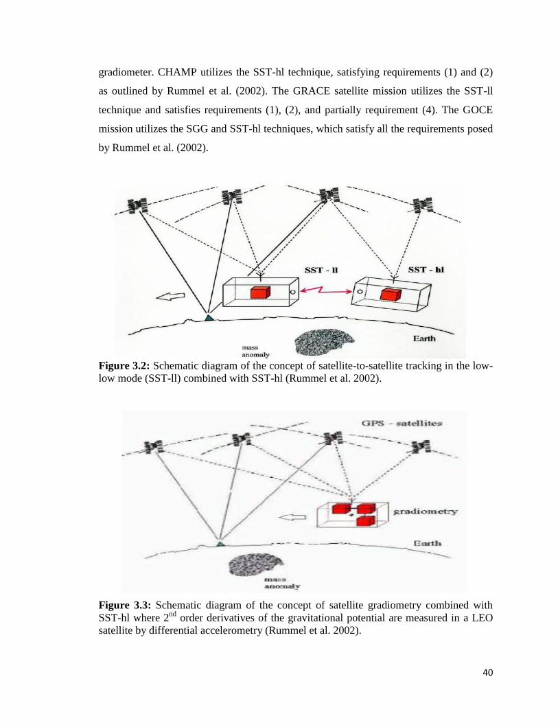
40
gradiometer. CHAMP utilizes the SST-hl technique, satisfying requirements (1) and (2)
as outlined by Rummel et al. (2002). The GRACE satellite mission utilizes the SST-ll
technique and satisfies requirements (1), (2), and partially requirement (4). The GOCE
mission utilizes the SGG and SST-hl techniques, which satisfy all the requirements posed
by Rummel et al. (2002).
Figure 3.2: Schematic diagram of the concept of satellite-to-satellite tracking in the low-
low mode (SST-ll) combined with SST-hl (Rummel et al. 2002).
Figure 3.3: Schematic diagram of the concept of satellite gradiometry combined with
SST-hl where 2nd
order derivatives of the gravitational potential are measured in a LEO
satellite by differential accelerometry (Rummel et al. 2002).

41
The CHAMP mission was put into orbit in order to measure the gravity and magnetic
fields of the Earth. It was in operation for over ten years with the mission ending on
September 19, 2010. The mission carried a GNSS receiver with continuous 3D tracking
capability and a precise accelerometer to measure non-gravitational forces. The orbit of
CHAMP was near circular with an 87 degree inclination and an altitude that decayed
from approximately 450 km to 300 km by the end of the mission. One of the first
developed GGMs using six months of CHAMP data improved the pre-CHAMP era GGM
GRIM5-S1 constructed using satellite orbit perturbations (Biancle et al. 2000) by almost
one order of magnitude up to degree and order 35 (Reigber et al. 2003; Pail et al. 2011).
The GRACE mission consists of two identical satellites following each other in the same
orbit by a separation distance of 200 km. The microwave Ka-band link via an inter-
satellite ranging system observes the relative motion of the twin satellites with very high
accuracy while the GNSS receivers measure the positions of the satellites, allowing
observations between the high and low orbiting satellites. Similarly to CHAMP, the
GRACE mission is also equipped with an on-board accelerometer to account for non-
gravitational forces. The mission has a near circular orbit with an 89 degree inclination at
an orbit altitude of 485 km. According to Pail et al. (2011), the GRACE-based GGMs
gained approximately two orders of magnitude in accuracy (i.e., 1 cm geoid error at
degree and order 100) as compared with GRIM5-S1.
In contrast to the CHAMP and GRACE missions, the SGG on board the GOCE mission
provides medium to short wavelength components of the gravity field as it measures the
second derivatives of the gravitational potential while the SST-hl mode is used to
determine the orbit and thus provides the long wavelength information of the gravity
field. In Chapter 2 it was shown that the gravitational potential can be expressed as a
spherical harmonic function (see Eq. (2.2)). Since the second derivate of the gravitational
potential is a functional of the potential, it too can be expressed in terms of a spherical
harmonic function. Such a function relates the GOCE observations to the spherical
harmonic coefficients that make up a GGM. Thus, by solving a large system of equations
via least squares the GGM coefficients can be deduced from GOCE observations. A
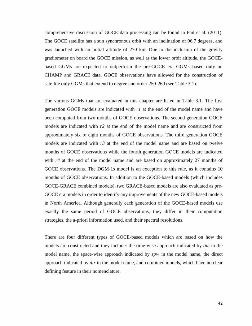
42
comprehensive discussion of GOCE data processing can be found in Pail et al. (2011).
The GOCE satellite has a sun synchronous orbit with an inclination of 96.7 degrees, and
was launched with an initial altitude of 270 km. Due to the inclusion of the gravity
gradiometer on board the GOCE mission, as well as the lower orbit altitude, the GOCE-
based GGMs are expected to outperform the pre-GOCE era GGMs based only on
CHAMP and GRACE data. GOCE observations have allowed for the construction of
satellite only GGMs that extend to degree and order 250-260 (see Table 3.1).
The various GGMs that are evaluated in this chapter are listed in Table 3.1. The first
generation GOCE models are indicated with r1 at the end of the model name and have
been computed from two months of GOCE observations. The second generation GOCE
models are indicated with r2 at the end of the model name and are constructed from
approximately six to eight months of GOCE observations. The third generation GOCE
models are indicated with r3 at the end of the model name and are based on twelve
months of GOCE observations while the fourth generation GOCE models are indicated
with r4 at the end of the model name and are based on approximately 27 months of
GOCE observations. The DGM-1s model is an exception to this rule, as it contains 10
months of GOCE observations. In addition to the GOCE-based models (which includes
GOCE-GRACE combined models), two GRACE-based models are also evaluated as pre-
GOCE era models in order to identify any improvements of the new GOCE-based models
in North America. Although generally each generation of the GOCE-based models use
exactly the same period of GOCE observations, they differ in their computation
strategies, the a-priori information used, and their spectral resolutions.
There are four different types of GOCE-based models which are based on how the
models are constructed and they include: the time-wise approach indicated by tim in the
model name, the space-wise approach indicated by spw in the model name, the direct
approach indicated by dir in the model name, and combined models, which have no clear
defining feature in their nomenclature.

43
Table 3.1 Global geopotential models.
Model nmax Data Source References
go_cons_gcf_2_dir_r4 260 GOCE direct approach based on 27.5
months of data and
go_cons_gcf_2_dir_r3 as a background
model
Bruinsma et al.
2010
go_cons_gcf_2_dir_r3 240 GOCE direct approach based on 12
months of data and
go_cons_gcf_2_dir_r2 as a background
model
Bruinsma et al.
2010
go_cons_gcf_2_dir_r2 240 GOCE direct approach based on 8
months of data and itg-grace2010s as a
background model
Bruinsma et al.
2010
go_cons_gcf_2_dir_r1 240 GOCE direct approach based on 2
months of data and eigen-5c as a
background model
Bruinsma et al.
2010
go_cons_gcf_2_tim_r4 250 GOCE time-wise approach based on 12
months of data
Pail et al. 2011
go_cons_gcf_2_tim_r3 250 GOCE time-wise approach based on 12
months of data
Pail et al. 2011
go_cons_gcf_2_tim_r2 250 GOCE time-wise approach based on 8
months of data
Pail et al. 2011
go_cons_gcf_2_tim_r1 224 GOCE time-wise approach based on 2
months of GOCE data
Pail et al.
2010a
goco03s 250 GOCE combined model based on 12
month of GOCE data, 7 years of GRACE
data, 8 years of CHAMP data and 5 years
of SLR
Mayer-Gürr et
al. 2012
goco02s 250 GOCE combined model based on 8
months of GOCE data, 7 years of
GRACE data, 8 years of CHAMP data
and 5 years of SLR
Goiginger et al.
2011
goco01s 224 GOCE combined model based on 2
months of GOCE data and 7 years of
GRACE data
Pail et al.
2010b
DGM-1s 250 GOCE combined model based on 10
months of GOCE data and 7 years of
GRACE data
Hashemi
Farahani et al.
2012
go_cons_gcf_2_spw_r2 240 GOCE space-wise approach based on 8
months of data
Migliaccio et
al. 2011
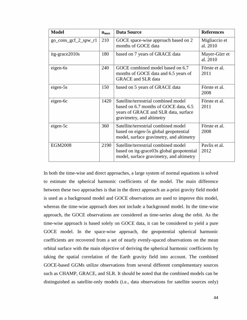
44
Model nmax Data Source References
go_cons_gcf_2_spw_r1 210 GOCE space-wise approach based on 2
months of GOCE data
Migliaccio et
al. 2010
itg-grace2010s 180 based on 7 years of GRACE data Mayer-Gürr et
al. 2010
eigen-6s 240 GOCE combined model based on 6.7
months of GOCE data and 6.5 years of
GRACE and SLR data
Förste et al.
2011
eigen-5s 150 based on 5 years of GRACE data Förste et al.
2008
eigen-6c 1420 Satellite/terrestrial combined model
based on 6.7 months of GOCE data, 6.5
years of GRACE and SLR data, surface
gravimetry, and altimetry
Förste et al.
2011
eigen-5c 360 Satellite/terrestrial combined model
based on eigen-5s global geopotential
model, surface gravimetry, and altimetry
Förste et al.
2008
EGM2008 2190 Satellite/terrestrial combined model
based on itg-grace03s global geopotential
model, surface gravimetry, and altimetry
Pavlis et al.
2012
In both the time-wise and direct approaches, a large system of normal equations is solved
to estimate the spherical harmonic coefficients of the model. The main difference
between these two approaches is that in the direct approach an a-prioi gravity field model
is used as a background model and GOCE observations are used to improve this model,
whereas the time-wise approach does not include a background model. In the time-wise
approach, the GOCE observations are considered as time-series along the orbit. As the
time-wise approach is based solely on GOCE data, it can be considered to yield a pure
GOCE model. In the space-wise approach, the geopotential spherical harmonic
coefficients are recovered from a set of nearly evenly-spaced observations on the mean
orbital surface with the main objective of deriving the spherical harmonic coefficients by
taking the spatial correlation of the Earth gravity field into account. The combined
GOCE-based GGMs utilize observations from several different complementary sources
such as CHAMP, GRACE, and SLR. It should be noted that the combined models can be
distinguished as satellite-only models (i.e., data observations for satellite sources only)
45
and satellite/terrestrial models (i.e., gravity observations are derived from surface
gravimetry and altimetry). A complete description about different methods used in the
development of GOCE-based models can be found in Pail et al. (2011).
3.3 GOCE Model Evaluation using GNSS/Levelling Data
Generally, comparisons with independent gravity field functionals are used to evaluate
the performance of the GOCE GGMs (Hirt et al. 2011). In order to estimate the external
accuracy (i.e., real geoid or gravity error) of a GGM three basic validation tools are
available, which are summarized in Table 3.2 (Gruber 2004). An important drawback of
comparisons with independent external datasets is that the results of comparisons are
reliable only when the quality of the external data set is high. Gruber (2004) uses
comparison with GNSS/levelling data and sea surface topography models to validate
GGMs based on CHAMP and GRACE coefficients, asserting that these methods can also
be used for the validation of GOCE models.
Gravity observations, such as the first radial derivative of the disturbing potential and the
first horizontal derivative of the disturbing potential (i.e., vertical deflections), contain
significant spectral power in the medium and higher frequencies (Schwarz 1985; Jekeli
1999), and therefore can be considered a complement to the evaluation of GGMs using
GNSS/levelling data (Gruber 2009; Ihde et al. 2010; Gruber et al. 2011; Hirt et al. 2011).
The GNSS/levelling validation method has been used in many studies for the evaluation
of a GGM, and has been used specifically to validate the very high-resolution global
model EGM2008 (Förste et al. 2009; Kotsakis and Katsambalos 2009; Jekeli et al. 2009).
The EGM2008 (Pavlis et al. 2012) is complete up to spherical harmonic degree and order
2160, and also provides additional spherical harmonic coefficients up to degree 2190.
This corresponds to a spatial resolution of 5 arc minutes, or approximately 9 km. Ince et
al. (2012) and Kotsakis and Katsambalos (2009) have used GNSS/levelling to test both
the absolute and relative agreement of geopotential models (i.e., GOCE and EGM2008,
respectively).
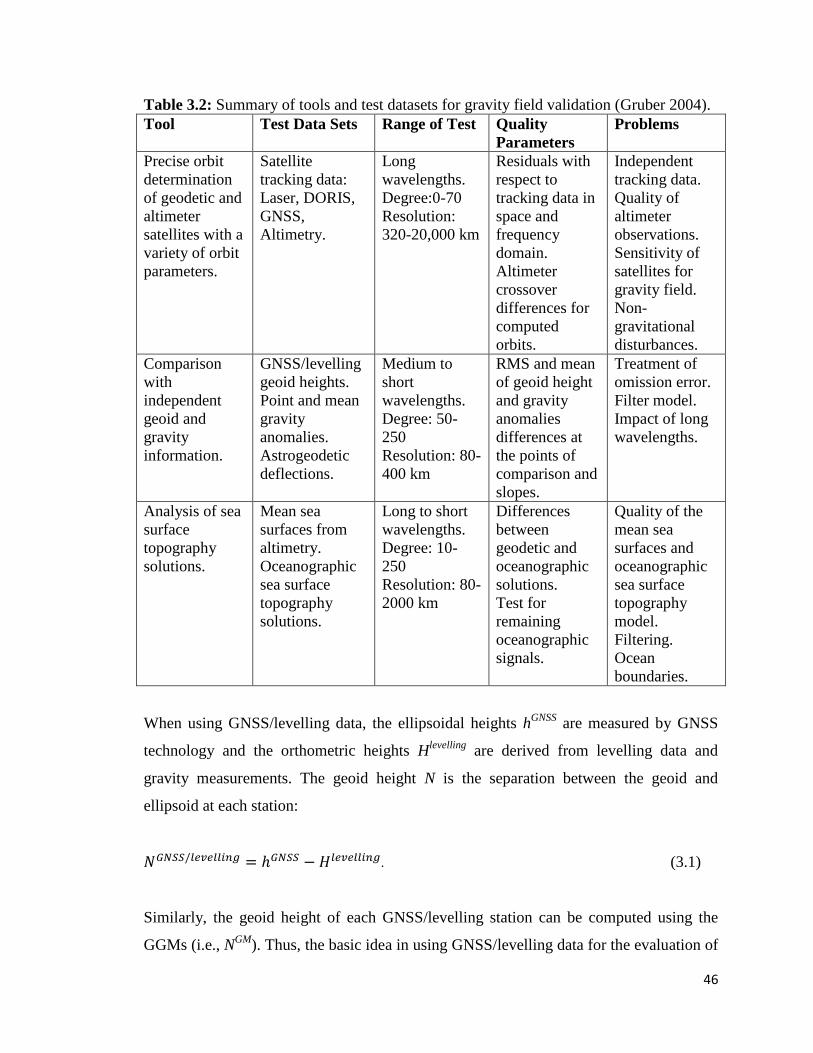
46
Table 3.2: Summary of tools and test datasets for gravity field validation (Gruber 2004).
Tool Test Data Sets Range of Test Quality
Parameters
Problems
Precise orbit
determination
of geodetic and
altimeter
satellites with a
variety of orbit
parameters.
Satellite
tracking data:
Laser, DORIS,
GNSS,
Altimetry.
Long
wavelengths.
Degree:0-70
Resolution:
320-20,000 km
Residuals with
respect to
tracking data in
space and
frequency
domain.
Altimeter
crossover
differences for
computed
orbits.
Independent
tracking data.
Quality of
altimeter
observations.
Sensitivity of
satellites for
gravity field.
Non-
gravitational
disturbances.
Comparison
with
independent
geoid and
gravity
information.
GNSS/levelling
geoid heights.
Point and mean
gravity
anomalies.
Astrogeodetic
deflections.
Medium to
short
wavelengths.
Degree: 50-
250
Resolution: 80-
400 km
RMS and mean
of geoid height
and gravity
anomalies
differences at
the points of
comparison and
slopes.
Treatment of
omission error.
Filter model.
Impact of long
wavelengths.
Analysis of sea
surface
topography
solutions.
Mean sea
surfaces from
altimetry.
Oceanographic
sea surface
topography
solutions.
Long to short
wavelengths.
Degree: 10-
250
Resolution: 80-
2000 km
Differences
between
geodetic and
oceanographic
solutions.
Test for
remaining
oceanographic
signals.
Quality of the
mean sea
surfaces and
oceanographic
sea surface
topography
model.
Filtering.
Ocean
boundaries.
When using GNSS/levelling data, the ellipsoidal heights hGNSS
are measured by GNSS
technology and the orthometric heights Hlevelling
are derived from levelling data and
gravity measurements. The geoid height N is the separation between the geoid and
ellipsoid at each station:
(3.1)
Similarly, the geoid height of each GNSS/levelling station can be computed using the
GGMs (i.e., NGM
). Thus, the basic idea in using GNSS/levelling data for the evaluation of
47
GGMs is the comparison of geoid heights obtained using a GGM (i.e., NGM
) and geoid
height obtained using GNSS/levelling data (i.e., NGNSS/levelling
).
A problem that occurs when using GNSS/levelling data or any other independent gravity
field functional to validate a GGM is the omission error. The GGMs are limited by their
maximum degree and order of coefficients, causing an omission error to always be
present due to the fact that the high-degree spectral content is missing (Hirt et al. 2011).
On the other hand, the terrestrial data to which the GGMs are compared contain the full
spectral signal. In order to appropriately compare the two data-sets they need to be
comparable in terms of their spectral content, which can be done by low-pass filtering of
the terrestrial data to remove high-frequency constituents (Gruber 2004), or by spectral
enhancement of the GGM-based functionals in the high and very high frequency range
(using a high resolution gravity field model such as EGM2008 and residual terrain
models (RTM)) so that it is more comparable with the full-spectrum terrestrial data (Hirt
et al. 2011). It should be noted that the GGM-based functionals can also be enhanced
with local gravity and topographic data using a remove-compute-restore scheme as
outlined in Chapter 2 in order to model the high frequency spectral content of the gravity
field. Low pass filtering using methods such as spectral filters, Gaussian filters, or least-
squares collocation (LSC) is a difficult task when the data is irregularly or scarcely
distributed, whereas the spectral enhancement method (SEM) can be used for GGM
validation as it is independent of the spatial distribution of the terrestrial data (Hirt et al.
2011).
The global magnitude of the omission error can also be estimated by means of a degree
variance model. The degree variance method provides an approximation described by the
degree variances of the geopotential (scaled to the geoid heights) to the global
contribution of the gravity signal (Heiskanen and Moritz 1967; Jekeli et al. 2009):
(
)
∑
(3.2)
48
where re is the radial distance to the ellipsoid and r
b is the radius of the bounding sphere.
As the full true gravity spectrum is unknown, in practice, instead of Eq. (3.2), degree
variance models fitted to the global gravity data are used or Kaula’s rule is applied
(Kaula 1966):
√∑
[ ], (3.3)
where nmax is the maximum degree and order of the geopotential model. It should be
noted that the degree variances method does not provide the spatial distribution of the
model’s omission error but yields only an average global value. There are also other
models that can be used for degree variances, such as, e.g., the Tscherning-Rapp model
(Tscherning and Rapp 1974).
Another error present that would cause a difference between the geoid undulations
derived using the GGM and the geoid undulations derived using GNSS/levelling is the
commission error of the GGM, which is the error that is propagated in the model through
the errors of the coefficients.
The standard deviation of the difference between the GGM derived geoid undulations and
the GNSS/levelling undulations contains the commission and omissions errors of the
spherical harmonic model, and also the errors in the GNSS and levelling data while the
mean difference accounts for the possible use of different ellipsoids and height datums
(Jekeli et al. 2009). The SEM should make the geoid undulations derived from GGMs
and the geoid undulations derived from GNSS/levelling as spectrally consistent as
possible, but will not entirely eliminate it, as even the SEM omission error estimates are
only good up to a finite degree and order.
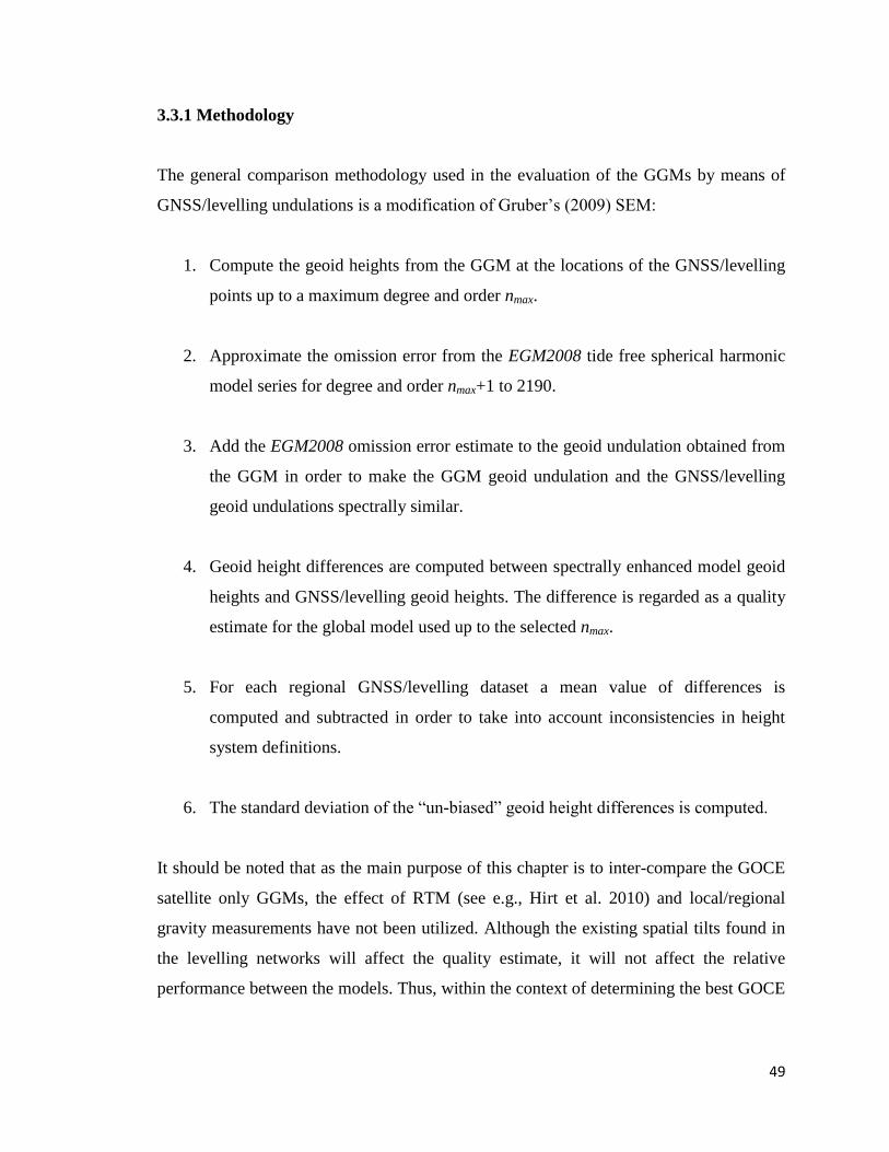
49
3.3.1 Methodology
The general comparison methodology used in the evaluation of the GGMs by means of
GNSS/levelling undulations is a modification of Gruber’s (2009) SEM:
1. Compute the geoid heights from the GGM at the locations of the GNSS/levelling
points up to a maximum degree and order nmax.
2. Approximate the omission error from the EGM2008 tide free spherical harmonic
model series for degree and order nmax+1 to 2190.
3. Add the EGM2008 omission error estimate to the geoid undulation obtained from
the GGM in order to make the GGM geoid undulation and the GNSS/levelling
geoid undulations spectrally similar.
4. Geoid height differences are computed between spectrally enhanced model geoid
heights and GNSS/levelling geoid heights. The difference is regarded as a quality
estimate for the global model used up to the selected nmax.
5. For each regional GNSS/levelling dataset a mean value of differences is
computed and subtracted in order to take into account inconsistencies in height
system definitions.
6. The standard deviation of the “un-biased” geoid height differences is computed.
It should be noted that as the main purpose of this chapter is to inter-compare the GOCE
satellite only GGMs, the effect of RTM (see e.g., Hirt et al. 2010) and local/regional
gravity measurements have not been utilized. Although the existing spatial tilts found in
the levelling networks will affect the quality estimate, it will not affect the relative
performance between the models. Thus, within the context of determining the best GOCE

50
GGM for height system unification and W0 determination, accounting for the spatial tilts
within the levelling networks, though ideally preferable, may be omitted.
The computation of geoid heights from spherical harmonic coefficients has been
performed using the harmonic_synth.f software (Holmes and Pavlis 2008). The zero-
degree term of the geoid height (see Eq. (2.51)) should be added to the computed geoid
heights from harmonic_synth.f. The GRS80 reference ellipsoid is used and the
conventional potential of the global equipotential surface is equal to W0=62,636,856.00
m2/s
2
as per the International Earth Rotation and Reference Systems Service (IERS,
2010) convention. Based on the GRS80 ellipsoid parameters and the IERS conventions,
the zero-degree term of the geoid height is computed as -43.7 cm.
3.3.2 GNSS/Levelling Benchmarks
GNSS/levelling benchmarks data sets for Canada were provided by the Geodetic Survey
Division (GSD) of Natural Resources Canada (NRCan). 1,315 data points with
orthometric heights in the Nov07 datum are used for the evaluation of the GOCE global
geopotential models in Canada. These data come from adjustments of the levelling
network on the Canadian mainland.
The GNSS ellipsoidal heights in this data set come from the 2006 adjustment of the GPS
SuperNet network in Canada (Craymer and Lapelle 1997) in ITRF2005 (Altamimi et al.
2007), epoch 2006.0. The ellipsoidal heights were corrected for the effect of the glacial
isostatic adjustment of the crust using a GNSS-derived crustal velocity model developed
by GSD (i.e., the National Velocity Model 1.0). Figure 3.4 shows the distribution of these
1,315 stations.
The effect of post glacial rebound or glacial isostatic adjustment in North America has an
effect on the geoid that ranges between 0.4-1.8 mm/yr, while the maximum vertical
crustal displacement may reach up to approximately 12 mm/yr in the Hudson Bay region
(Rangelova 2007).
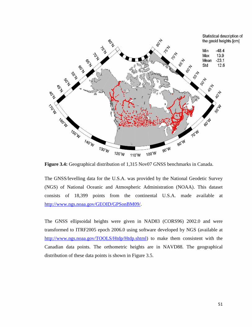
51
Figure 3.4: Geographical distribution of 1,315 Nov07 GNSS benchmarks in Canada.
The GNSS/levelling data for the U.S.A. was provided by the National Geodetic Survey
(NGS) of National Oceanic and Atmospheric Administration (NOAA). This dataset
consists of 18,399 points from the continental U.S.A. made available at
http://www.ngs.noaa.gov/GEOID/GPSonBM09/.
The GNSS ellipsoidal heights were given in NAD83 (CORS96) 2002.0 and were
transformed to ITRF2005 epoch 2006.0 using software developed by NGS (available at
http://www.ngs.noaa.gov/TOOLS/Htdp/Htdp.shtml) to make them consistent with the
Canadian data points. The orthometric heights are in NAVD88. The geographical
distribution of these data points is shown in Figure 3.5.
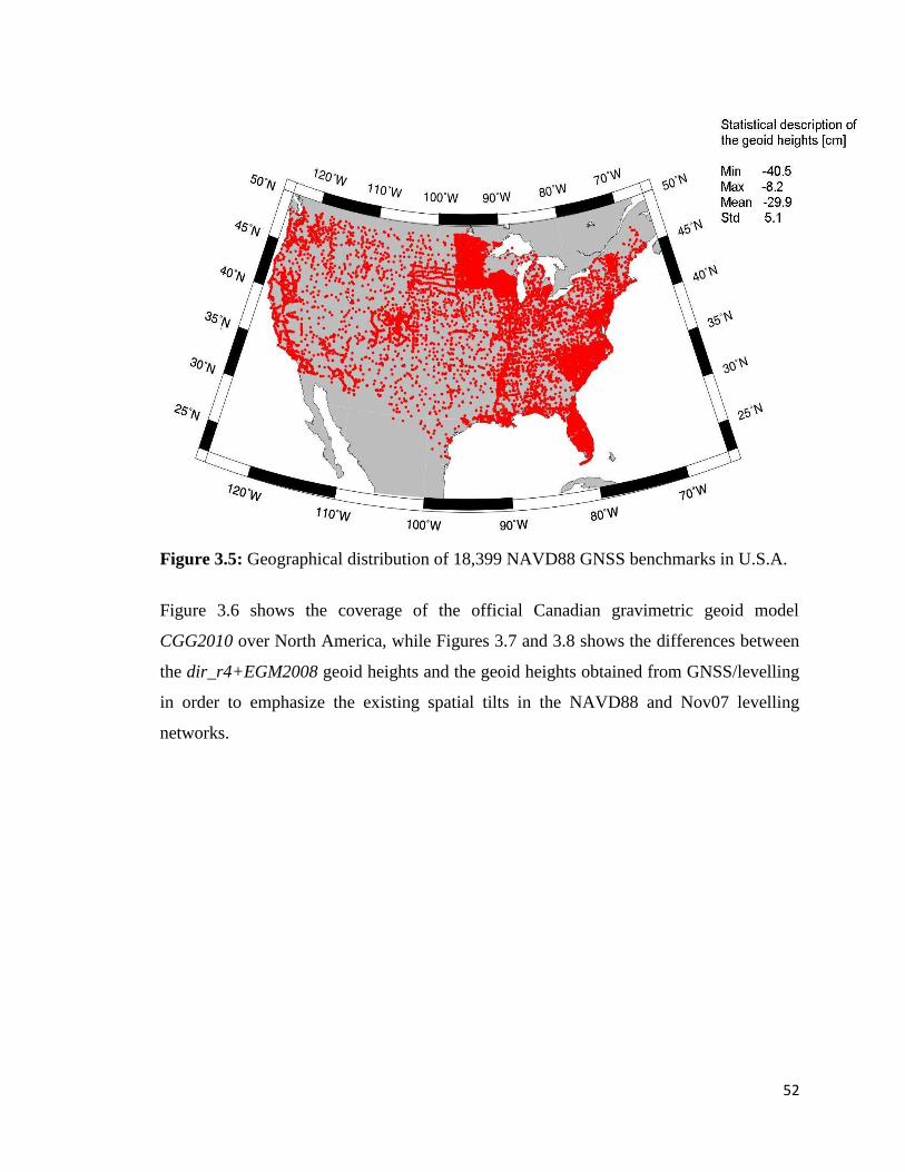
52
Figure 3.5: Geographical distribution of 18,399 NAVD88 GNSS benchmarks in U.S.A.
Figure 3.6 shows the coverage of the official Canadian gravimetric geoid model
CGG2010 over North America, while Figures 3.7 and 3.8 shows the differences between
the dir_r4+EGM2008 geoid heights and the geoid heights obtained from GNSS/levelling
in order to emphasize the existing spatial tilts in the NAVD88 and Nov07 levelling
networks.
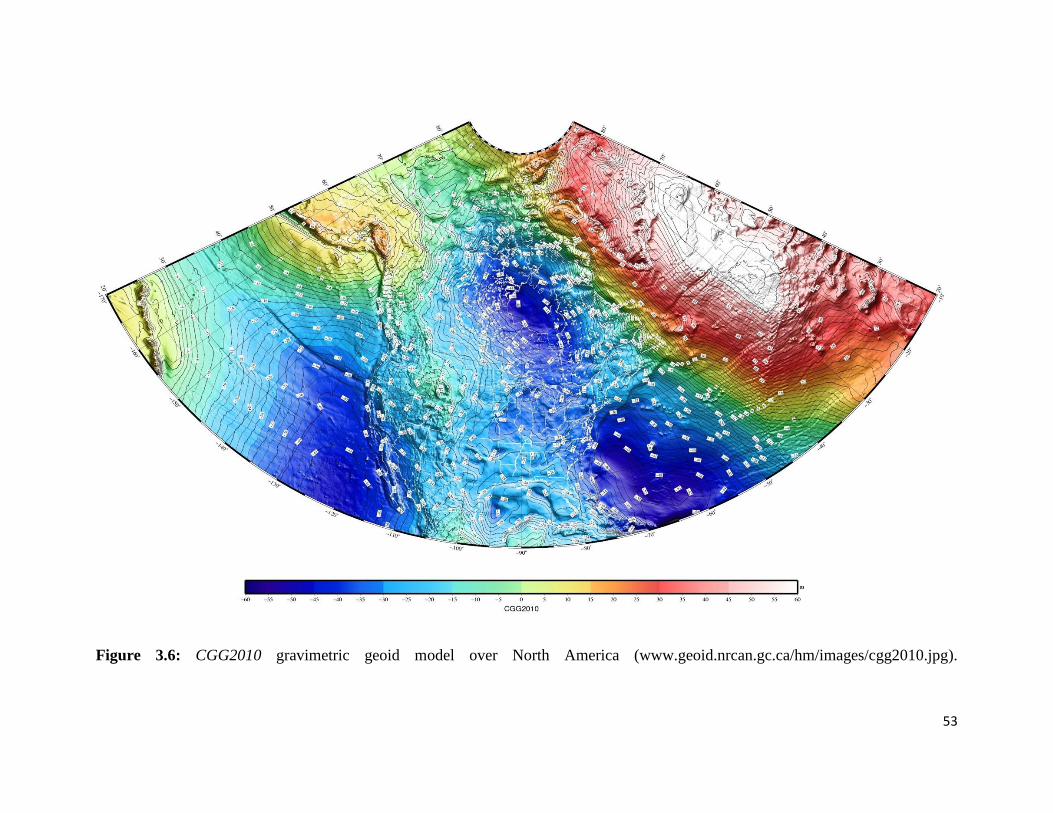
53
Figure 3.6: CGG2010 gravimetric geoid model over North America (www.geoid.nrcan.gc.ca/hm/images/cgg2010.jpg).
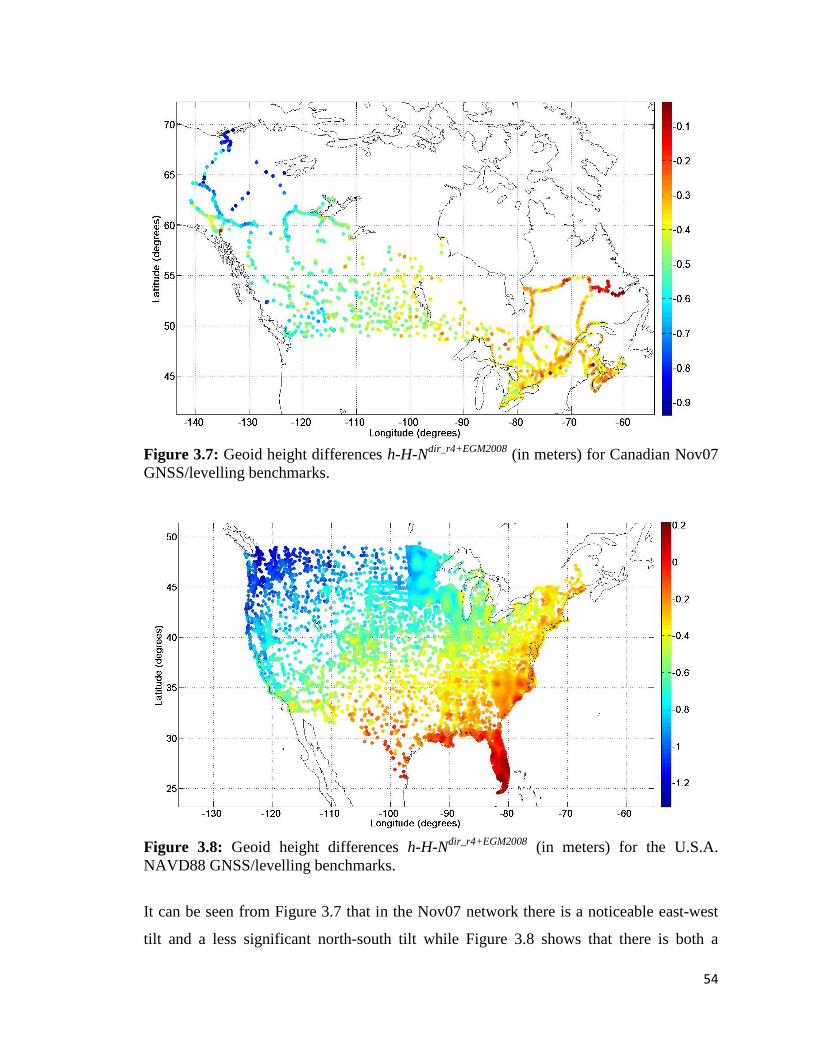
54
Figure 3.7: Geoid height differences h-H-N
dir_r4+EGM2008 (in meters) for Canadian Nov07
GNSS/levelling benchmarks.
Figure 3.8: Geoid height differences h-H-N
dir_r4+EGM2008 (in meters) for the U.S.A.
NAVD88 GNSS/levelling benchmarks.
It can be seen from Figure 3.7 that in the Nov07 network there is a noticeable east-west
tilt and a less significant north-south tilt while Figure 3.8 shows that there is both a

55
significant east-west tilt and north-south tilt present in the U.S.A. NAVD88 levelling
network, which can be attributed to the accumulation of systematic levelling errors and
the difference of the mean sea levels between the west and east coasts of North America.
3.4 Results and Discussion
This section describes the evaluation results by means of geoid height comparisons in
Canada and the U.S.A. Absolute comparisons are presented and the performance of the
GOCE models in different spectral bands is investigated. The omission error of the
GGMs is approximated using the high resolution model EGM2008.
3.4.1 Global Cumulative Geoid Error from Degree Variances
The cumulative global geoid error can be evaluated from the error degree variances of a
GGM. The total cumulative geoid error is the square root of the sum of the error degree
variances. Figure 3.9 shows the cumulative geoid errors at different degrees of truncation
for the third and fourth generation direct and time-wise GOCE GGMs. As the gravity
field model error curves are derived from error estimates as a result of a least squares
solution (i.e., utilized in order obtain the spherical harmonic coefficients), they can be
regarded as “internal” error estimates. From Figure 3.9, it can be seen that at degree and
order 200, which corresponds to a spatial resolution of approximately 100 km, the dir_r4
model has a cumulative geoid error of approximately 1 cm, while the tim_r4 model has a
cumulative geoid error of approximately 4 cm. This is an improvement over the third
generation models, where dir_r3 has a cumulative geoid error of approximately 3 cm and
the tim_r3 has a cumulative geoid error of approximately 6 cm at degree and order 200.
Thus, with the release of the dir_r4 model, it appears that the GOCE mission objective of
obtaining the geoid with a global accuracy of 1-2 cm at a spatial resolution of 100 km has
been achieved. With longer time series of GOCE observations, the time-wise approach
may also achieve a global cumulative geoid error of 1-2 cm at truncation degree 200. In
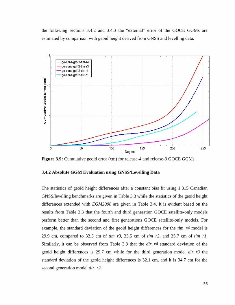
56
the following sections 3.4.2 and 3.4.3 the “external” error of the GOCE GGMs are
estimated by comparison with geoid height derived from GNSS and levelling data.
Figure 3.9: Cumulative geoid error (cm) for release-4 and release-3 GOCE GGMs.
3.4.2 Absolute GGM Evaluation using GNSS/Levelling Data
The statistics of geoid height differences after a constant bias fit using 1,315 Canadian
GNSS/levelling benchmarks are given in Table 3.3 while the statistics of the geoid height
differences extended with EGM2008 are given in Table 3.4. It is evident based on the
results from Table 3.3 that the fourth and third generation GOCE satellite-only models
perform better than the second and first generations GOCE satellite-only models. For
example, the standard deviation of the geoid height differences for the tim_r4 model is
29.9 cm, compared to 32.3 cm of tim_r3, 33.5 cm of tim_r2, and 35.7 cm of tim_r1.
Similarly, it can be observed from Table 3.3 that the dir_r4 standard deviation of the
geoid height differences is 29.7 cm while for the third generation model dir_r3 the
standard deviation of the geoid height differences is 32.1 cm, and it is 34.7 cm for the
second generation model dir_r2.
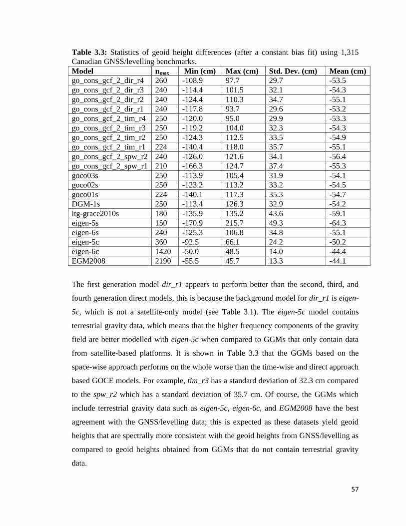
57
Table 3.3: Statistics of geoid height differences (after a constant bias fit) using 1,315
Canadian GNSS/levelling benchmarks.
Model nmax Min (cm) Max (cm) Std. Dev. (cm) Mean (cm)
go_cons_gcf_2_dir_r4 260 -108.9 97.7 29.7 -53.5
go_cons_gcf_2_dir_r3 240 -114.4 101.5 32.1 -54.3
go_cons_gcf_2_dir_r2 240 -124.4 110.3 34.7 -55.1
go_cons_gcf_2_dir_r1 240 -117.8 93.7 29.6 -53.2
go_cons_gcf_2_tim_r4 250 -120.0 95.0 29.9 -53.3
go_cons_gcf_2_tim_r3 250 -119.2 104.0 32.3 -54.3
go_cons_gcf_2_tim_r2 250 -124.3 112.5 33.5 -54.9
go_cons_gcf_2_tim_r1 224 -140.4 118.0 35.7 -55.1
go_cons_gcf_2_spw_r2 240 -126.0 121.6 34.1 -56.4
go_cons_gcf_2_spw_r1 210 -166.3 124.7 37.4 -55.3
goco03s 250 -113.9 105.4 31.9 -54.1
goco02s 250 -123.2 113.2 33.2 -54.5
goco01s 224 -140.1 117.3 35.3 -54.7
DGM-1s 250 -113.4 126.3 32.9 -54.2
itg-grace2010s 180 -135.9 135.2 43.6 -59.1
eigen-5s 150 -170.9 215.7 49.3 -64.3
eigen-6s 240 -125.3 106.8 34.8 -55.1
eigen-5c 360 -92.5 66.1 24.2 -50.2
eigen-6c 1420 -50.0 48.5 14.0 -44.4
EGM2008 2190 -55.5 45.7 13.3 -44.1
The first generation model dir_r1 appears to perform better than the second, third, and
fourth generation direct models, this is because the background model for dir_r1 is eigen-
5c, which is not a satellite-only model (see Table 3.1). The eigen-5c model contains
terrestrial gravity data, which means that the higher frequency components of the gravity
field are better modelled with eigen-5c when compared to GGMs that only contain data
from satellite-based platforms. It is shown in Table 3.3 that the GGMs based on the
space-wise approach performs on the whole worse than the time-wise and direct approach
based GOCE models. For example, tim_r3 has a standard deviation of 32.3 cm compared
to the spw_r2 which has a standard deviation of 35.7 cm. Of course, the GGMs which
include terrestrial gravity data such as eigen-5c, eigen-6c, and EGM2008 have the best
agreement with the GNSS/levelling data; this is expected as these datasets yield geoid
heights that are spectrally more consistent with the geoid heights from GNSS/levelling as
compared to geoid heights obtained from GGMs that do not contain terrestrial gravity
data.

58
Table 3.4: Statistics of geoid height differences (after a constant bias fit) with EGM2008
extended GGMs to degree and order 2,190 using 1,315 Canadian GNSS/levelling
benchmarks.
Model nmax Min (cm) Max (cm) Std. Dev. (cm) Mean (cm)
go_cons_gcf_2_dir_r4 260 -74.7 45.0 16.6 -45.5
go_cons_gcf_2_dir_r3 240 -69.3 55.4 19.7 -45.3
go_cons_gcf_2_dir_r2 240 -85.0 63.5 23.2 -46.1
go_cons_gcf_2_dir_r1 240 -53.2 47.7 14.4 -44.1
go_cons_gcf_2_tim_r4 250 -66.7 45.3 16.8 -45.3
go_cons_gcf_2_tim_r3 250 -72.1 54.8 20.6 -46.3
go_cons_gcf_2_tim_r2 250 -106.9 58.2 22.4 -46.9
go_cons_gcf_2_tim_r1 224 -63.3 49.7 21.8 -45.4
go_cons_gcf_2_spw_r2 240 -82.9 62.3 21.7 -47.3
go_cons_gcf_2_spw_r1 210 -70.3 66.9 22.4 -44.8
goco03s 250 -74.7 55.7 20.0 -46.1
goco02s 250 -107.8 55.9 22.1 -46.5
goco01s 224 -63.5 52.4 21.2 -45.1
DGM-1s 250 -89.8 52.4 22.8 -46.2
itg-grace2010s 180 -71.4 89.9 23.6 -44.4
eigen-5s 150 -142.2 121.7 32.9 -49.6
eigen-6s 240 -87.3 66.8 23.4 -46.1
eigen-5c 360 -74.5 54.8 18.1 -46.1
eigen-6c 1420 -50.4 48.1 13.7 -44.1
EGM2008 2190 -55.5 45.7 13.3 -44.1
Likewise, results presented in Table 3.4 show more or less the same trends as the results
from Table 3.3. The standard deviations and the mean value of the geoid height
differences have decreased in general for most of the GOCE-based GGMs, since the
models have been extended with EGM2008, which incorporates terrestrial gravity data.
For example, for tim_r3 the mean value of the geoid height difference from Table 3.3 is
54.3 cm and it is 46.3 once extended with EGM2008. The approximate effect of the
GOCE omission error on the mean geoid height difference is thus 8 cm. When comparing
the mean geoid height differences between Table 3.3 and 3.4, it can be seen that the
effect of the omission error it is greater for GRACE based models, which is at the dm-
level. This has do with the fact that GRACE based models are only expanded to a
maximum degree and order of 150 to 180 while GOCE based models are usually
expanded to a maximum degree and order of 240 to 260. Here it is evident that including
the SGG on-board the GOCE mission has helped to resolve higher frequencies of the
gravity field when compared with pre-GOCE missions such as GRACE.
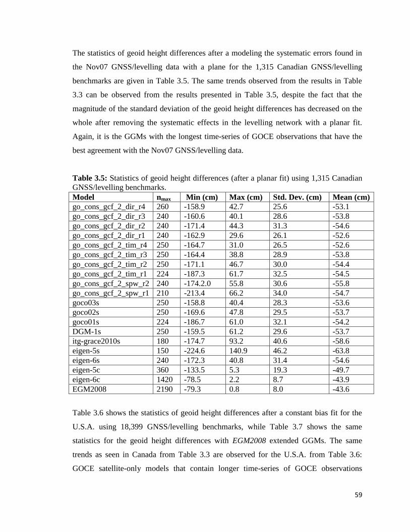
59
The statistics of geoid height differences after a modeling the systematic errors found in
the Nov07 GNSS/levelling data with a plane for the 1,315 Canadian GNSS/levelling
benchmarks are given in Table 3.5. The same trends observed from the results in Table
3.3 can be observed from the results presented in Table 3.5, despite the fact that the
magnitude of the standard deviation of the geoid height differences has decreased on the
whole after removing the systematic effects in the levelling network with a planar fit.
Again, it is the GGMs with the longest time-series of GOCE observations that have the
best agreement with the Nov07 GNSS/levelling data.
Table 3.5: Statistics of geoid height differences (after a planar fit) using 1,315 Canadian
GNSS/levelling benchmarks.
Model nmax Min (cm) Max (cm) Std. Dev. (cm) Mean (cm)
go_cons_gcf_2_dir_r4 260 -158.9 42.7 25.6 -53.1
go_cons_gcf_2_dir_r3 240 -160.6 40.1 28.6 -53.8
go_cons_gcf_2_dir_r2 240 -171.4 44.3 31.3 -54.6
go_cons_gcf_2_dir_r1 240 -162.9 29.6 26.1 -52.6
go_cons_gcf_2_tim_r4 250 -164.7 31.0 26.5 -52.6
go_cons_gcf_2_tim_r3 250 -164.4 38.8 28.9 -53.8
go_cons_gcf_2_tim_r2 250 -171.1 46.7 30.0 -54.4
go_cons_gcf_2_tim_r1 224 -187.3 61.7 32.5 -54.5
go_cons_gcf_2_spw_r2 240 -174.2.0 55.8 30.6 -55.8
go_cons_gcf_2_spw_r1 210 -213.4 66.2 34.0 -54.7
goco03s 250 -158.8 40.4 28.3 -53.6
goco02s 250 -169.6 47.8 29.5 -53.7
goco01s 224 -186.7 61.0 32.1 -54.2
DGM-1s 250 -159.5 61.2 29.6 -53.7
itg-grace2010s 180 -174.7 93.2 40.6 -58.6
eigen-5s 150 -224.6 140.9 46.2 -63.8
eigen-6s 240 -172.3 40.8 31.4 -54.6
eigen-5c 360 -133.5 5.3 19.3 -49.7
eigen-6c 1420 -78.5 2.2 8.7 -43.9
EGM2008 2190 -79.3 0.8 8.0 -43.6
Table 3.6 shows the statistics of geoid height differences after a constant bias fit for the
U.S.A. using 18,399 GNSS/levelling benchmarks, while Table 3.7 shows the same
statistics for the geoid height differences with EGM2008 extended GGMs. The same
trends as seen in Canada from Table 3.3 are observed for the U.S.A. from Table 3.6:
GOCE satellite-only models that contain longer time-series of GOCE observations
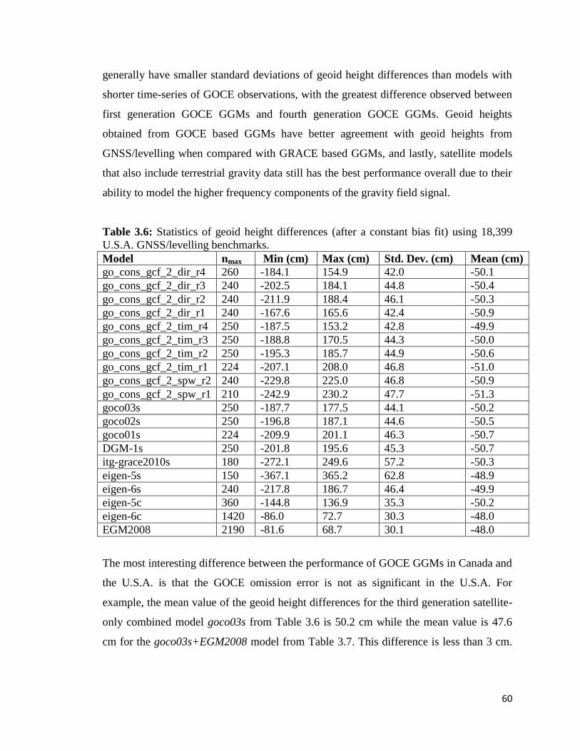
60
generally have smaller standard deviations of geoid height differences than models with
shorter time-series of GOCE observations, with the greatest difference observed between
first generation GOCE GGMs and fourth generation GOCE GGMs. Geoid heights
obtained from GOCE based GGMs have better agreement with geoid heights from
GNSS/levelling when compared with GRACE based GGMs, and lastly, satellite models
that also include terrestrial gravity data still has the best performance overall due to their
ability to model the higher frequency components of the gravity field signal.
Table 3.6: Statistics of geoid height differences (after a constant bias fit) using 18,399
U.S.A. GNSS/levelling benchmarks.
Model nmax Min (cm) Max (cm) Std. Dev. (cm) Mean (cm)
go_cons_gcf_2_dir_r4 260 -184.1 154.9 42.0 -50.1
go_cons_gcf_2_dir_r3 240 -202.5 184.1 44.8 -50.4
go_cons_gcf_2_dir_r2 240 -211.9 188.4 46.1 -50.3
go_cons_gcf_2_dir_r1 240 -167.6 165.6 42.4 -50.9
go_cons_gcf_2_tim_r4 250 -187.5 153.2 42.8 -49.9
go_cons_gcf_2_tim_r3 250 -188.8 170.5 44.3 -50.0
go_cons_gcf_2_tim_r2 250 -195.3 185.7 44.9 -50.6
go_cons_gcf_2_tim_r1 224 -207.1 208.0 46.8 -51.0
go_cons_gcf_2_spw_r2 240 -229.8 225.0 46.8 -50.9
go_cons_gcf_2_spw_r1 210 -242.9 230.2 47.7 -51.3
goco03s 250 -187.7 177.5 44.1 -50.2
goco02s 250 -196.8 187.1 44.6 -50.5
goco01s 224 -209.9 201.1 46.3 -50.7
DGM-1s 250 -201.8 195.6 45.3 -50.7
itg-grace2010s 180 -272.1 249.6 57.2 -50.3
eigen-5s 150 -367.1 365.2 62.8 -48.9
eigen-6s 240 -217.8 186.7 46.4 -49.9
eigen-5c 360 -144.8 136.9 35.3 -50.2
eigen-6c 1420 -86.0 72.7 30.3 -48.0
EGM2008 2190 -81.6 68.7 30.1 -48.0
The most interesting difference between the performance of GOCE GGMs in Canada and
the U.S.A. is that the GOCE omission error is not as significant in the U.S.A. For
example, the mean value of the geoid height differences for the third generation satellite-
only combined model goco03s from Table 3.6 is 50.2 cm while the mean value is 47.6
cm for the goco03s+EGM2008 model from Table 3.7. This difference is less than 3 cm.
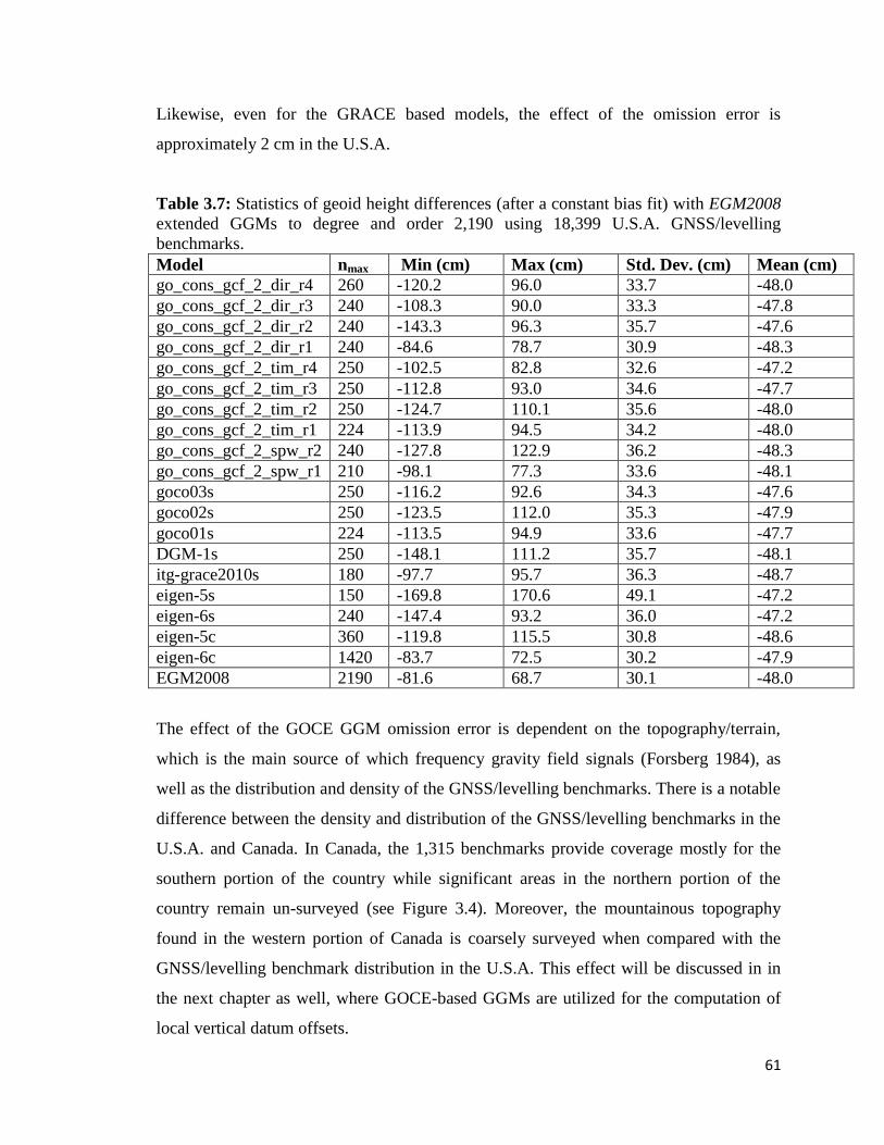
61
Likewise, even for the GRACE based models, the effect of the omission error is
approximately 2 cm in the U.S.A.
Table 3.7: Statistics of geoid height differences (after a constant bias fit) with EGM2008
extended GGMs to degree and order 2,190 using 18,399 U.S.A. GNSS/levelling
benchmarks.
Model nmax Min (cm) Max (cm) Std. Dev. (cm) Mean (cm)
go_cons_gcf_2_dir_r4 260 -120.2 96.0 33.7 -48.0
go_cons_gcf_2_dir_r3 240 -108.3 90.0 33.3 -47.8
go_cons_gcf_2_dir_r2 240 -143.3 96.3 35.7 -47.6
go_cons_gcf_2_dir_r1 240 -84.6 78.7 30.9 -48.3
go_cons_gcf_2_tim_r4 250 -102.5 82.8 32.6 -47.2
go_cons_gcf_2_tim_r3 250 -112.8 93.0 34.6 -47.7
go_cons_gcf_2_tim_r2 250 -124.7 110.1 35.6 -48.0
go_cons_gcf_2_tim_r1 224 -113.9 94.5 34.2 -48.0
go_cons_gcf_2_spw_r2 240 -127.8 122.9 36.2 -48.3
go_cons_gcf_2_spw_r1 210 -98.1 77.3 33.6 -48.1
goco03s 250 -116.2 92.6 34.3 -47.6
goco02s 250 -123.5 112.0 35.3 -47.9
goco01s 224 -113.5 94.9 33.6 -47.7
DGM-1s 250 -148.1 111.2 35.7 -48.1
itg-grace2010s 180 -97.7 95.7 36.3 -48.7
eigen-5s 150 -169.8 170.6 49.1 -47.2
eigen-6s 240 -147.4 93.2 36.0 -47.2
eigen-5c 360 -119.8 115.5 30.8 -48.6
eigen-6c 1420 -83.7 72.5 30.2 -47.9
EGM2008 2190 -81.6 68.7 30.1 -48.0
The effect of the GOCE GGM omission error is dependent on the topography/terrain,
which is the main source of which frequency gravity field signals (Forsberg 1984), as
well as the distribution and density of the GNSS/levelling benchmarks. There is a notable
difference between the density and distribution of the GNSS/levelling benchmarks in the
U.S.A. and Canada. In Canada, the 1,315 benchmarks provide coverage mostly for the
southern portion of the country while significant areas in the northern portion of the
country remain un-surveyed (see Figure 3.4). Moreover, the mountainous topography
found in the western portion of Canada is coarsely surveyed when compared with the
GNSS/levelling benchmark distribution in the U.S.A. This effect will be discussed in in
the next chapter as well, where GOCE-based GGMs are utilized for the computation of
local vertical datum offsets.
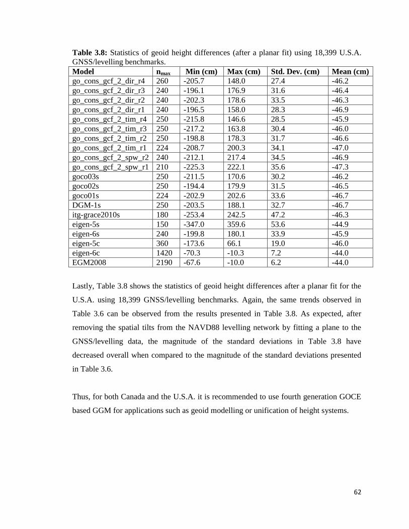
62
Table 3.8: Statistics of geoid height differences (after a planar fit) using 18,399 U.S.A.
GNSS/levelling benchmarks.
Model nmax Min (cm) Max (cm) Std. Dev. (cm) Mean (cm)
go_cons_gcf_2_dir_r4 260 -205.7 148.0 27.4 -46.2
go_cons_gcf_2_dir_r3 240 -196.1 176.9 31.6 -46.4
go_cons_gcf_2_dir_r2 240 -202.3 178.6 33.5 -46.3
go_cons_gcf_2_dir_r1 240 -196.5 158.0 28.3 -46.9
go_cons_gcf_2_tim_r4 250 -215.8 146.6 28.5 -45.9
go_cons_gcf_2_tim_r3 250 -217.2 163.8 30.4 -46.0
go_cons_gcf_2_tim_r2 250 -198.8 178.3 31.7 -46.6
go_cons_gcf_2_tim_r1 224 -208.7 200.3 34.1 -47.0
go_cons_gcf_2_spw_r2 240 -212.1 217.4 34.5 -46.9
go_cons_gcf_2_spw_r1 210 -225.3 222.1 35.6 -47.3
goco03s 250 -211.5 170.6 30.2 -46.2
goco02s 250 -194.4 179.9 31.5 -46.5
goco01s 224 -202.9 202.6 33.6 -46.7
DGM-1s 250 -203.5 188.1 32.7 -46.7
itg-grace2010s 180 -253.4 242.5 47.2 -46.3
eigen-5s 150 -347.0 359.6 53.6 -44.9
eigen-6s 240 -199.8 180.1 33.9 -45.9
eigen-5c 360 -173.6 66.1 19.0 -46.0
eigen-6c 1420 -70.3 -10.3 7.2 -44.0
EGM2008 2190 -67.6 -10.0 6.2 -44.0
Lastly, Table 3.8 shows the statistics of geoid height differences after a planar fit for the
U.S.A. using 18,399 GNSS/levelling benchmarks. Again, the same trends observed in
Table 3.6 can be observed from the results presented in Table 3.8. As expected, after
removing the spatial tilts from the NAVD88 levelling network by fitting a plane to the
GNSS/levelling data, the magnitude of the standard deviations in Table 3.8 have
decreased overall when compared to the magnitude of the standard deviations presented
in Table 3.6.
Thus, for both Canada and the U.S.A. it is recommended to use fourth generation GOCE
based GGM for applications such as geoid modelling or unification of height systems.

63
3.4.3 Performance of the GGMs in Different Spectral Bands
In order to evaluate the GOCE GGM performance in different spectral bands the models
are truncated at a selected degree (i.e., from degree and order 10 to the maximum degree
and order of the model in intervals of 10 degrees). The spherical harmonic coefficient of
each model from the truncation degree to the maximum degree and order of the model is
replaced by EGM2008 coefficients, and the models are additionally extended to degree
and order 2190 (i.e., the nmax of EGM2008). Figure 3.10 shows the performance of the
time-wise GOCE GGMs (i.e., the pure GOCE models) and two pre-GOCE era GRACE
satellite-only models for Canada while Figure 3.14 shows the same for the U.S.A. Similar
trends are observed for both countries. Firstly, an improvement of each successive release
of GOCE models due to increasing length of GOCE observations included in each
consecutive model generation is observed (i.e., tim_r4 performs better than tim_r3 and
tim_r3 performs better than tim_r2 etc.). Secondly, the GRACE based GGMs lose their
signal in lower degrees, while the GOCE models show more signal content in higher
spectral bands, which can be attributed to the inclusion of 2 to 27 months of GOCE
observations. Thus, it can be concluded that the inclusion of even 2 months of GOCE
observations will provide additional information about the gravity field in both Canada
and the U.S.A.
In Figure 3.11 the performance of the direct GOCE GGMs are shown along with the
background models eigen-5c for dir_r1 and itg-grace2010s for dir_r2 while dir_r2 is
used as the background model for dir_r3. Similarly, Figure 3.15 shows the same models
for U.S.A. Of course, the same trends as seen in Figures 3.10 and 3.14 with the time-wise
GOCE models are also seen with the direct GOCE models. The interesting feature to note
is that the dir_r1 model in Canada shows improvement with respect to eigen-5c, which
can be attributed to the inclusion of 2 months of GOCE data. However, in the U.S.A this
cannot be observed.
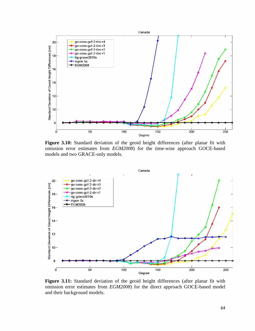
64
Figure 3.10: Standard deviation of the geoid height differences (after planar fit with
omission error estimates from EGM2008) for the time-wise approach GOCE-based
models and two GRACE-only models.
Figure 3.11: Standard deviation of the geoid height differences (after planar fit with
omission error estimates from EGM2008) for the direct approach GOCE-based model
and their background models.
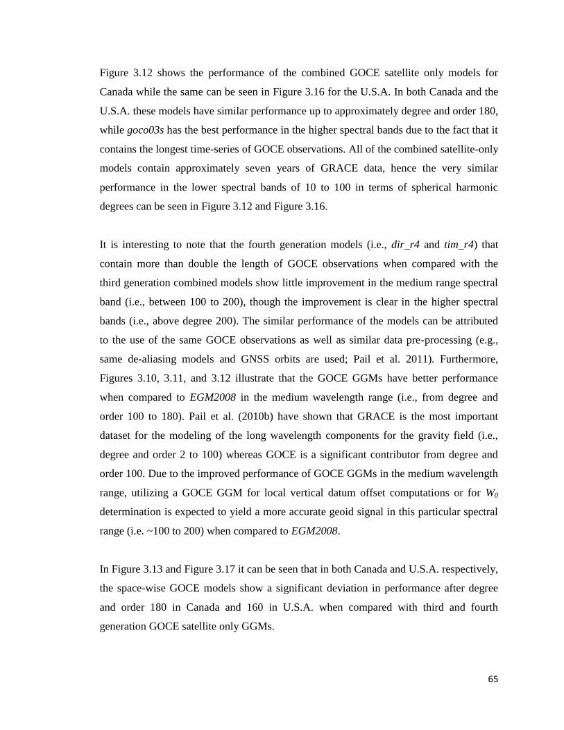
65
Figure 3.12 shows the performance of the combined GOCE satellite only models for
Canada while the same can be seen in Figure 3.16 for the U.S.A. In both Canada and the
U.S.A. these models have similar performance up to approximately degree and order 180,
while goco03s has the best performance in the higher spectral bands due to the fact that it
contains the longest time-series of GOCE observations. All of the combined satellite-only
models contain approximately seven years of GRACE data, hence the very similar
performance in the lower spectral bands of 10 to 100 in terms of spherical harmonic
degrees can be seen in Figure 3.12 and Figure 3.16.
It is interesting to note that the fourth generation models (i.e., dir_r4 and tim_r4) that
contain more than double the length of GOCE observations when compared with the
third generation combined models show little improvement in the medium range spectral
band (i.e., between 100 to 200), though the improvement is clear in the higher spectral
bands (i.e., above degree 200). The similar performance of the models can be attributed
to the use of the same GOCE observations as well as similar data pre-processing (e.g.,
same de-aliasing models and GNSS orbits are used; Pail et al. 2011). Furthermore,
Figures 3.10, 3.11, and 3.12 illustrate that the GOCE GGMs have better performance
when compared to EGM2008 in the medium wavelength range (i.e., from degree and
order 100 to 180). Pail et al. (2010b) have shown that GRACE is the most important
dataset for the modeling of the long wavelength components for the gravity field (i.e.,
degree and order 2 to 100) whereas GOCE is a significant contributor from degree and
order 100. Due to the improved performance of GOCE GGMs in the medium wavelength
range, utilizing a GOCE GGM for local vertical datum offset computations or for W0
determination is expected to yield a more accurate geoid signal in this particular spectral
range (i.e. ~100 to 200) when compared to EGM2008.
In Figure 3.13 and Figure 3.17 it can be seen that in both Canada and U.S.A. respectively,
the space-wise GOCE models show a significant deviation in performance after degree
and order 180 in Canada and 160 in U.S.A. when compared with third and fourth
generation GOCE satellite only GGMs.
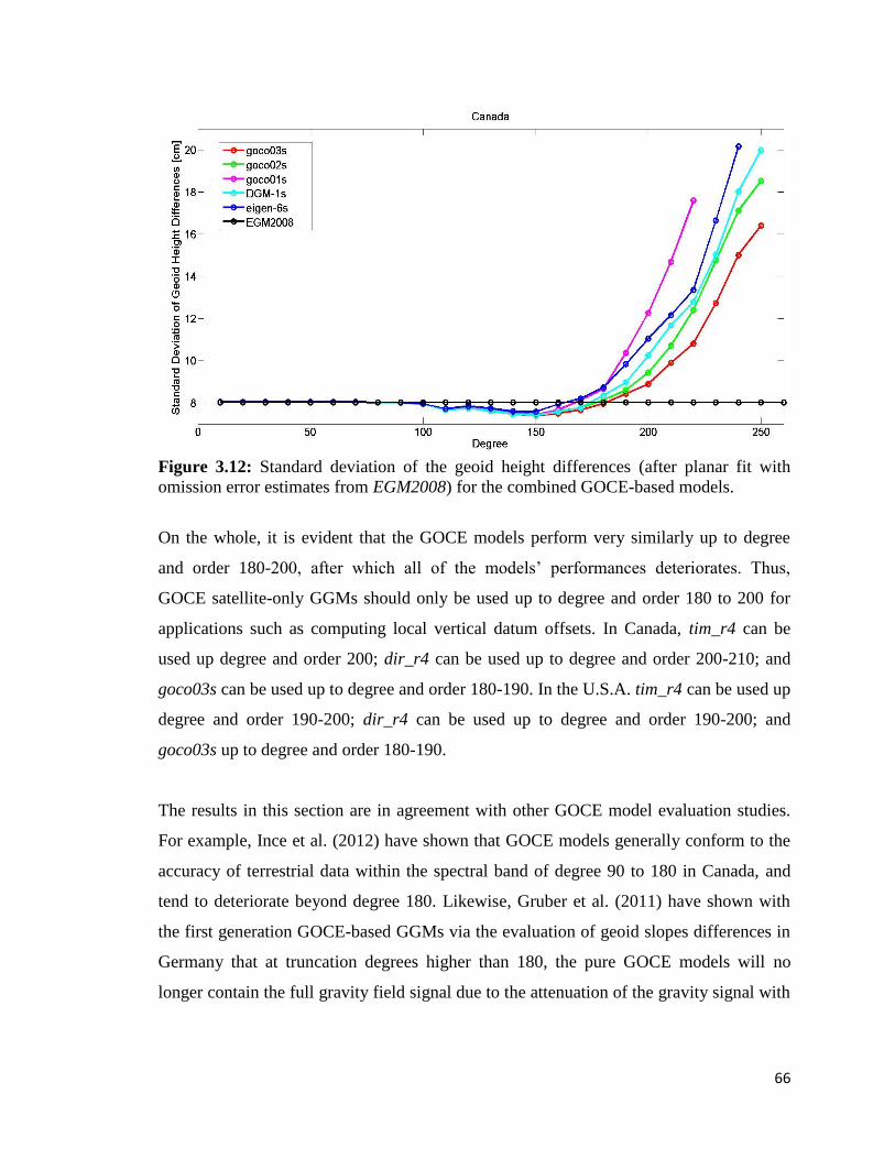
66
Figure 3.12: Standard deviation of the geoid height differences (after planar fit with
omission error estimates from EGM2008) for the combined GOCE-based models.
On the whole, it is evident that the GOCE models perform very similarly up to degree
and order 180-200, after which all of the models’ performances deteriorates. Thus,
GOCE satellite-only GGMs should only be used up to degree and order 180 to 200 for
applications such as computing local vertical datum offsets. In Canada, tim_r4 can be
used up degree and order 200; dir_r4 can be used up to degree and order 200-210; and
goco03s can be used up to degree and order 180-190. In the U.S.A. tim_r4 can be used up
degree and order 190-200; dir_r4 can be used up to degree and order 190-200; and
goco03s up to degree and order 180-190.
The results in this section are in agreement with other GOCE model evaluation studies.
For example, Ince et al. (2012) have shown that GOCE models generally conform to the
accuracy of terrestrial data within the spectral band of degree 90 to 180 in Canada, and
tend to deteriorate beyond degree 180. Likewise, Gruber et al. (2011) have shown with
the first generation GOCE-based GGMs via the evaluation of geoid slopes differences in
Germany that at truncation degrees higher than 180, the pure GOCE models will no
longer contain the full gravity field signal due to the attenuation of the gravity signal with
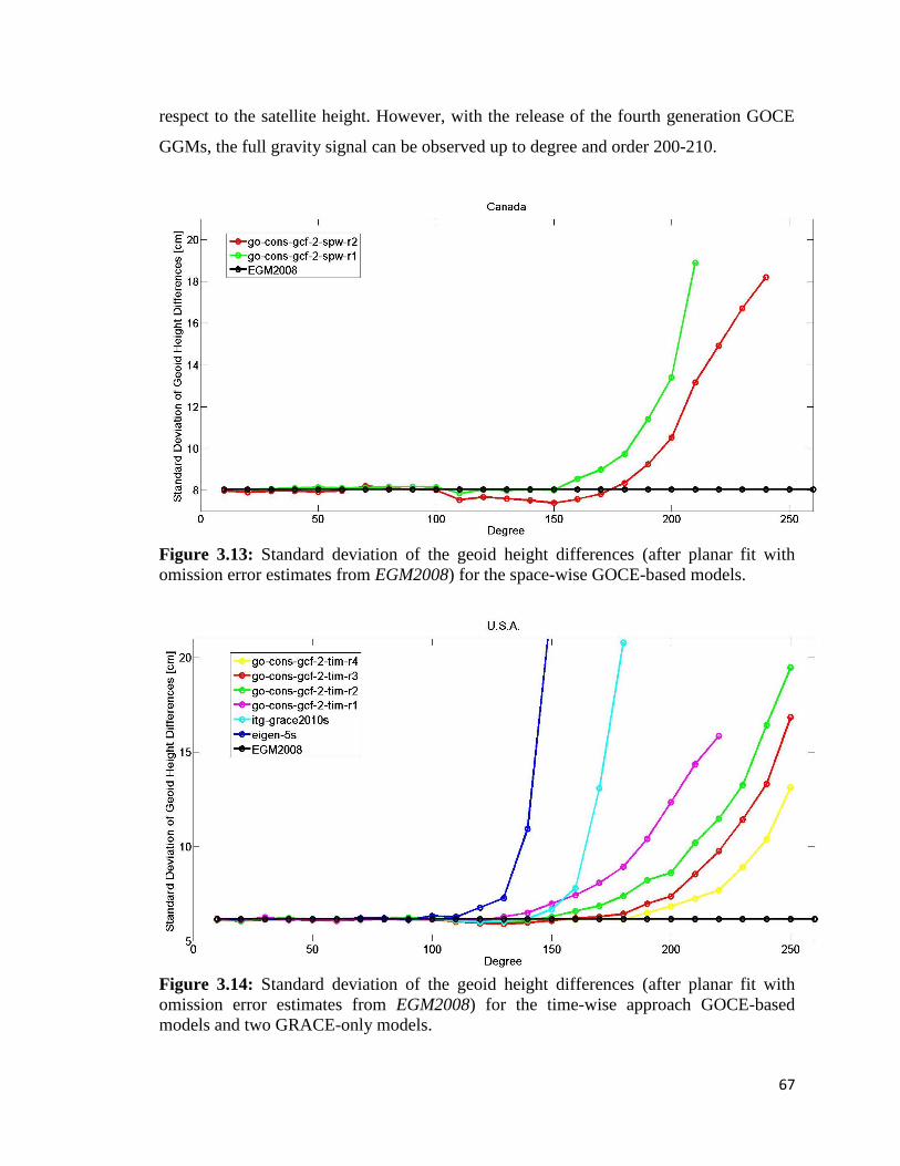
67
respect to the satellite height. However, with the release of the fourth generation GOCE
GGMs, the full gravity signal can be observed up to degree and order 200-210.
Figure 3.13: Standard deviation of the geoid height differences (after planar fit with
omission error estimates from EGM2008) for the space-wise GOCE-based models.
Figure 3.14: Standard deviation of the geoid height differences (after planar fit with
omission error estimates from EGM2008) for the time-wise approach GOCE-based
models and two GRACE-only models.
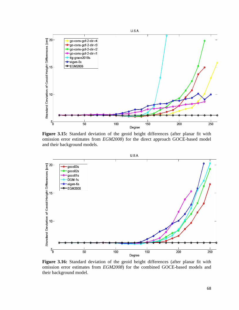
68
Figure 3.15: Standard deviation of the geoid height differences (after planar fit with
omission error estimates from EGM2008) for the direct approach GOCE-based model
and their background models.
Figure 3.16: Standard deviation of the geoid height differences (after planar fit with
omission error estimates from EGM2008) for the combined GOCE-based models and
their background model.
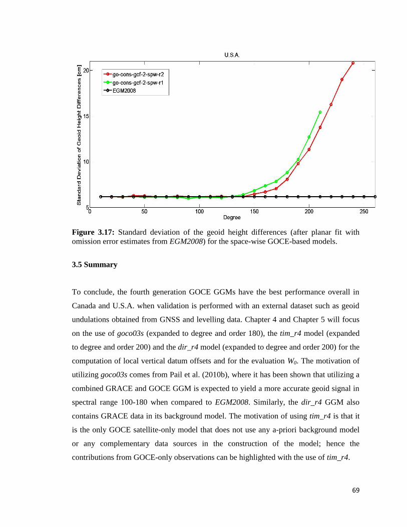
69
Figure 3.17: Standard deviation of the geoid height differences (after planar fit with
omission error estimates from EGM2008) for the space-wise GOCE-based models.
3.5 Summary
To conclude, the fourth generation GOCE GGMs have the best performance overall in
Canada and U.S.A. when validation is performed with an external dataset such as geoid
undulations obtained from GNSS and levelling data. Chapter 4 and Chapter 5 will focus
on the use of goco03s (expanded to degree and order 180), the tim_r4 model (expanded
to degree and order 200) and the dir_r4 model (expanded to degree and order 200) for the
computation of local vertical datum offsets and for the evaluation W0. The motivation of
utilizing goco03s comes from Pail et al. (2010b), where it has been shown that utilizing a
combined GRACE and GOCE GGM is expected to yield a more accurate geoid signal in
spectral range 100-180 when compared to EGM2008. Similarly, the dir_r4 GGM also
contains GRACE data in its background model. The motivation of using tim_r4 is that it
is the only GOCE satellite-only model that does not use any a-priori background model
or any complementary data sources in the construction of the model; hence the
contributions from GOCE-only observations can be highlighted with the use of tim_r4.

70
From the absolute comparison of geoid height differences the ultra high resolution GGMs
EGM2008 and eigen_6c show better performance than the rest of the models for both
Canada and U.S.A. This is because both Canada and U.S.A. are gravimetrically well
surveyed and thus have a good coverage of terrestrial gravity measurements that can
adequately model the higher frequency signals of the gravity field. These terrestrial
gravity measurements were used in the development of the ultra-high resolution GGMs
and this is the main reason for the superior performance of these models in Canada and
U.S.A. The opposite situation is observed in the regions with poor coverage and/or bad
quality of terrestrial gravity measurements. For example, the geoid accuracy of
EGM2008 is at the dm-level over large parts of Asia, Africa, South America, and
Antarctica due to the lack of high resolution terrestrial data in these regions (Hirt et al.
2012). It is for these regions, where dense terrestrial gravity observations are missing,
that GOCE is expected to contribute most significantly.
Lastly, accounting for the effect of RTM can improve the comparison results between the
geoid height differences, which can play an important role in the evaluation of GGMs in
mountainous regions (Hirt et al. 2011). The contribution higher frequency gravity field
content from RTM may be considered for future GGM evaluation studies for North
America.
71
CHAPTER 4
ESTIMATING VERTICAL DATUM OFFSETS IN NORTH AMERICA WITH
GOCE GLOBAL GEOPOTENTIAL MODELS
4.1 Introduction
Vertical datum realization and unification has been amongst one of the main topics of
research in geodesy, and has been discussed in detail over the last three decades by
Colombo (1980), Rummel and Teunissen (1988), Heck and Rummel (1990), Rapp and
Balasubramania (1992), Xu (1992), Rummel and Ilk (1995), Jekeli (2000), and Burša et
al. (2004), among others. These studies have illustrated that by determining the potential
value of a LVD, it is possible to relate different datums around the world, and also to
define a world vertical datum.
In theory, the choice of the datum point (or datum origin) and its potential value can be
arbitrary, but as heights are in practice given with respect to the MSL, the datum points
are usually chosen at or close to tide gauges (tied to the vertical control network), and the
adopted potential value at these points are chosen such that the zero level coincides with
the MSL. However, due to the fact that the MSL varies both spatially and temporally, the
zero level defined from the long term averaging of tide gauge records results in different
reference surface between datum zones as illustrated in Figure 4.1, where O(j)
and O(k)
are the datum origin points that define the reference surfaces in datum zone j and datum
k; hA and hB are the ellipsoidal heights of point A and point B obtained from GNSS; H(j)
A
and H(k)
B are the orthometric heights obtained from leveling in datum zone j and datum
zone k at points A and B, respectively; N(j)
A and N(k)
B are the geoid undulations obtained
from GNSS/levelling in datum zone j and datum zone k at points A and B, respectively;
and δN(j)
A and δN(k)
B are the local vertical datum offsets with respect to the global
conventional geoid W0. It should be noted that the geoid and the ellipsoidal surfaces
illustrated in Figure 4.1 are in reality not parallel to each other.
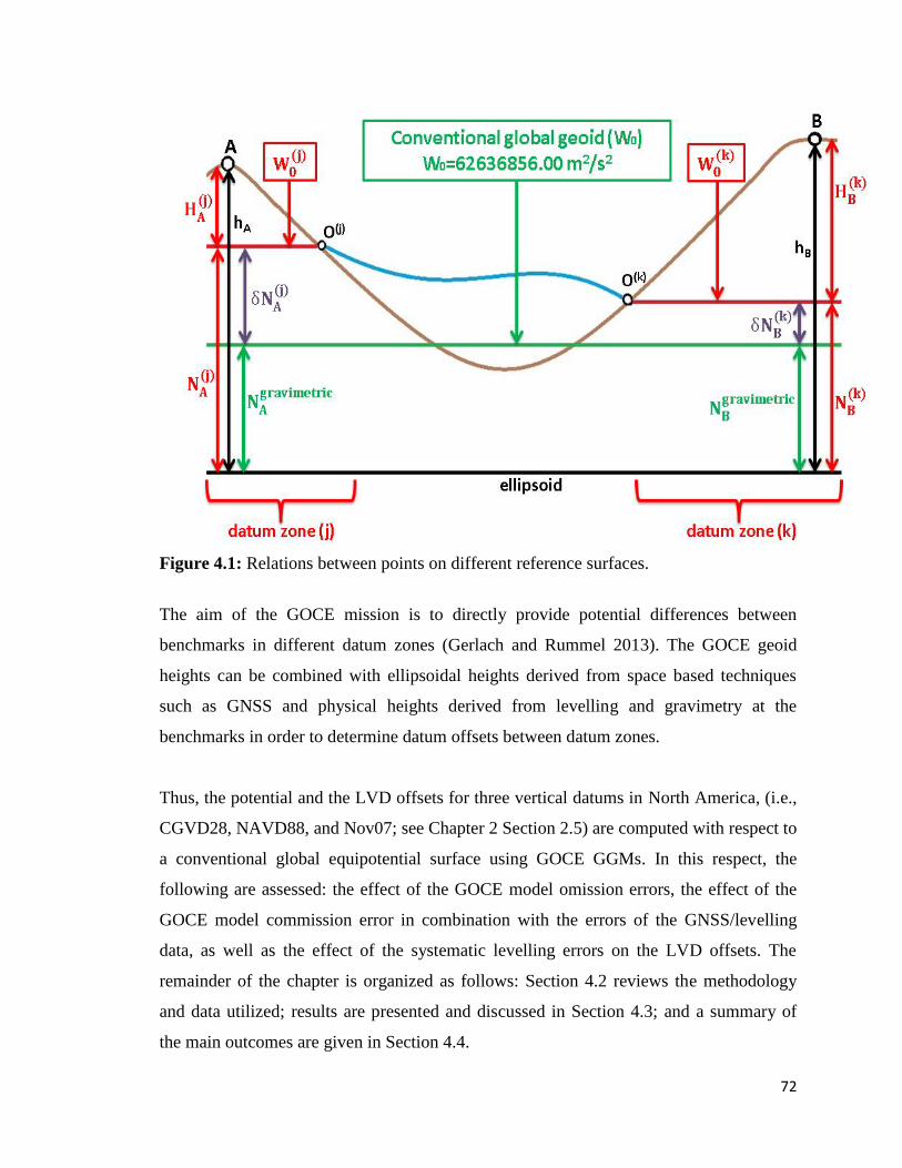
72
Figure 4.1: Relations between points on different reference surfaces.
The aim of the GOCE mission is to directly provide potential differences between
benchmarks in different datum zones (Gerlach and Rummel 2013). The GOCE geoid
heights can be combined with ellipsoidal heights derived from space based techniques
such as GNSS and physical heights derived from levelling and gravimetry at the
benchmarks in order to determine datum offsets between datum zones.
Thus, the potential and the LVD offsets for three vertical datums in North America, (i.e.,
CGVD28, NAVD88, and Nov07; see Chapter 2 Section 2.5) are computed with respect to
a conventional global equipotential surface using GOCE GGMs. In this respect, the
following are assessed: the effect of the GOCE model omission errors, the effect of the
GOCE model commission error in combination with the errors of the GNSS/levelling
data, as well as the effect of the systematic levelling errors on the LVD offsets. The
remainder of the chapter is organized as follows: Section 4.2 reviews the methodology
and data utilized; results are presented and discussed in Section 4.3; and a summary of
the main outcomes are given in Section 4.4.
73
4.2 Methodology
According to Rummel (2001) there are three basic approaches or methods available for
the connection of different datum zones:
1) direct connection by levelling and gravimetry,
2) oceanographic approaches, and
3) indirect connection by solving the geodetic boundary value problem (GBVP).
Option (1) is not suitable for global height unification since it can only be used on
continents while option (2) relies on the fact that the mean dynamic topography (MDT;
i.e., the height of the sea surface above the geoid) should be precisely known at co-
located datum point tide gauges for which the MDT difference between tide gauges from
different datum zones would correspond of the datum or height offset between the datum
zones (Gerlach and Rummel 2013). The MDT can be obtained from oceanographic
models or from altimetry determined mean sea surface (MSS) heights and a precise
gravimetric geoid model. However, altimetry determined sea surface heights in coastal
regions tend to have poor accuracy due to the fact that the altimetry signal is likely to be
contaminated by the land portion of the coastline.
Following the work of Rummel and Teunissen (1988) (i.e., option (3)), one begins with
the assumption that there are J+1 different LVD zones (j)
, i { , ,…,J}, which refer to
different tide gauges and consequently have different reference surfaces. Choosing one of
these datums as a reference datum, the height unification method aims to link all the other
datum zones to the reference datum 0.
The geopotential difference of datum zone j can be evaluated by
(4.1)
where W0 refers to the gravity potential of the selected reference datum and W ( )
refers to
the gravity potential of the LVD in datum zone j.
74
The offset of the local zero height surface from the reference level surface is:
. (4.2)
The solution to the GBVP for points P is given by:
∬ {
}
(4.3)
The Δg( ) are biased gravity anomalies derived from terrestrial data and the unbiased
gravity anomalies are obtained after correcting for the datum offset of datum zone j:
(4.4)
The Δg( ) represents the gravity anomaly on the topographic surface reduced to the zero
height surface in the zone j using the orthometric height H(j)
using:
(4.5)
where gP is the measured gravity at the Earth’s surface at a point P and γ0 is the normal
gravity evaluated at the ellipsoid. It follows that Δg( )
is biased since H(j)
is biased due to
the unknown offset between the height reference surface through datum point Oj and the
geoid. The term 2
δW( ) is interpreted as the “free-air” reduction which is used to reduce
the gravity anomaly Δg( ) from the local zero height surface to the level surface defined
by the W0 value. Of course, it is not possible to correct the biased gravity anomalies
before one is able to determine δW( ). Equation (4.3) is inserted in Bruns’s equation (see
Chapter 2, Eq. (2.32)):
, (4.6)
75
where ΔW0=W0-U0.
Thus, the observation equation of the geoid height can be given by:
(
)
∬ {
}
∑
∬
(4.7)
The first bracketed term on the right hand side in Eq. (4.7) is the zero-order term (see
Chapter 2, Eq. (2.51)).
The third term in Eq. (4.7) is the solution of the Stokes integral with the local gravity
anomalies (i.e., geoid height determined using Stokes integral):
∬
(4.8)
The fourth term represents the indirect effect of the terrain on the geoid. Using
S
2π∬ S(ψ
)d
the fourth term in Eq. (4.7) can be written as:
∑
∬
∑
∑
(4.9)
Substituting Eq. (4.2), Eq. (2.51), Eq. (4.8) and Eq. (4.9), Eq. (4.7) becomes:
∑
(4.10)
where δN( ) is the local datum offset, and ∑ S
δN is the indirect bias term. Thus, the
height reference surface of a specific datum zone deviates from the unbiased geoid not
only due to its own datum offset (i.e., the direct bias term) but also due to the integration
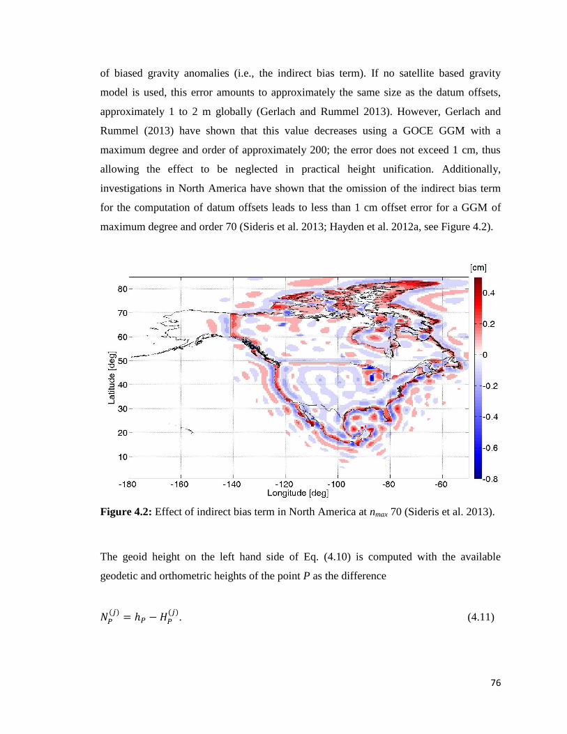
76
of biased gravity anomalies (i.e., the indirect bias term). If no satellite based gravity
model is used, this error amounts to approximately the same size as the datum offsets,
approximately 1 to 2 m globally (Gerlach and Rummel 2013). However, Gerlach and
Rummel (2013) have shown that this value decreases using a GOCE GGM with a
maximum degree and order of approximately 200; the error does not exceed 1 cm, thus
allowing the effect to be neglected in practical height unification. Additionally,
investigations in North America have shown that the omission of the indirect bias term
for the computation of datum offsets leads to less than 1 cm offset error for a GGM of
maximum degree and order 70 (Sideris et al. 2013; Hayden et al. 2012a, see Figure 4.2).
Figure 4.2: Effect of indirect bias term in North America at nmax 70 (Sideris et al. 2013).
The geoid height on the left hand side of Eq. (4.10) is computed with the available
geodetic and orthometric heights of the point P as the difference
. (4.11)
77
The indirect bias term can be omitted as it has been shown in Figure 4.2 that its effect is
less than one centimeter in North America for GGMs used up to at least degree and order
70. Thus, Eq. (4.10) can be re-written as
(4.12)
The geopotential difference can then be computed by multiplying the computed offset by
the normal gravity on the ellipsoid:
(4.13)
Preferably, one would obtain the geoid height NP in Eq. (4.12) from a high-accuracy
satellite-only GGM, such as the GOCE-based models, and evaluate the medium- to short-
wavelength geoid signals using local gravity anomalies and topographic information in a
remove-restore computational scheme (see Chapter 2, Section 2.6). The Canadian official
geoid model CGG2010 (Huang and Véronneau 2013) and the U.S.A. official geoid
model USGG2012 (www.ngs.noaa.gov/GEOID/USGG2012) are both examples of
optimal combinations of a satellite-only GGM, local gravity, and topographic
information. The CGG2010 geoid heights are available on a 2’ by 2’ grid for a region that
covers 20N to 80N and -170W to -10W while the USGG2012 geoid heights are
available on a 1’ by 1’ grid for a region that covers 24N to 58N and -130W to -60W
for mainland U.S.A.; in addition coverage for Alaska, Hawaii, Guam and Northern
Mariana Islands, Puerto Rico, U.S.A. Virgin Islands, and the American Samoa is also
available. Hence, CGG2010 can be utilized to assess the magnitude of the omission error
of the GOCE GGM in a large part of North America (see Chapter 3, Figure 3.6).
One may also use the EGM2008 (Pavlis et al. 2012) model to approximate the omission
error of the GOCE models. However, EGM2008 is not able to model a gravity field
signal with half-wavelengths smaller than 9 km. The global average omission error is
approximately 4 cm when the geoid is computed using EGM2008, although it can be
larger in mountainous terrain (Jekeli 2009). In other words, due to the fact that the

78
topography of the Earth is the main source of high-frequency gravity field signals
(Forsberg 1984), the effect of the omission error in low-lying terrain will tend to be
smaller than in mountainous regions (see, e.g., Hirt et al. 2010). Moreover, the residual
terrain model (RTM) technique (Forsberg and Tscherning 1981; Forsberg 1984; Forsberg
1985) can be used to model the high-frequency signals not provided by the EGM2008
model. When using the RTM technique a digital terrain model representing the Earth’s
topography is referred to a long-wavelength reference surface, which removes the low-
frequency components of the digital terrain model already implied by the GGM (Hirt et
al. 2010). However, in regions with sufficient terrestrial gravity data coverage, such as
Canada or the U.S.A., the remove-compute-restore method allows for a more accurate
modelling of the high frequency components of the gravity field. Thus, CGG2010 and
USGG2012 are better candidates than EGM2008 to quantify the contribution of the high
frequencies of the gravity field that are not modelled by the GOCE GGMs. The
gravimetric geoid model developed by Ince et al. (2012), though not an official geoid
model of Canada, can be considered an updated gravimetric geoid model with respect to
CGG2010, as it uses the third generation direct GOCE model for the long wavelength
contributions of the gravity field, and can also be used to quantify omission errors.
It should be emphasized that CGG2010 and USGG2012 are not completely independent
from EGM2008. EGM2008 uses the high-quality Canadian and U.S.A. local gravity
information that is used in the computation of CGG2010 and USGG2012. Conversely,
CGG2010 utilizes goco01s (Pail et al. 2010) and EGM2008 from degree 2 to 224 using a
weighted averaging based on the coefficient standard deviations and EGM2008 up to
degree and order 2190 (Huang J., Natural Resources Canada, personal communication,
November 29, 2012). In USGG2012, the goco02s model substitutes the GRACE model
that went into making EGM2008 by applying a cosine taper to blend the goco02s
coefficients with those of EGM2008, starting at degree and order 100 and ending at
degree and order 200, which produces a modified reference model reflecting GOCE data
for the mid-wavelengths of the gravity field signal (Roman D., National Geodetic Survey,
personal communication, March 21, 2013). Therefore, one can expect that the effect of

79
the GOCE omitted signal on the LVD offsets will not differ significantly when it is
evaluated by means of EGM2008, CGG2010, or USGG2012.
4.2.1 Sources of Error affecting LVD Offset Computations
Systematic and random measurement errors, as well as the omission and commission
errors from the gravity field models will affect the LVD offsets computed from
GNSS/levelling information. According to Kotsakis et al. (2011), a biased LVD offset
(i.e., an offset value that differs from the true LVD offset value) may result in the
presence of systematic effects and spatially correlated errors in the height data. In such a
case, h -
-N will not follow the typical trend of a constant offset; rather it may reveal
spatial tilts or even a more complex oscillatory pattern over the network of
GNSS/levelling benchmarks.
Systematic errors that can contribute to biased LVD offsets comprise of datum
inconsistencies between the ellipsoidal heights and the geoid heights, which result from
the use of different reference ellipsoids in the geoid model and ellipsoidal heights.
Additionally, geometrical distortions in the levelling height data due to over-constraining
the LVD to several tide gauge stations (e.g., CGVD28), long and medium wavelength
errors in the geoid model, accumulated systematic errors in the levelling network (Entin
1959), improper modelling of temporal height variations, the inconsistent treatment of
permanent tide in the geoid, physical and ellipsoidal heights (Ekman 1989; Mäkinen and
Ihde 2009), and the uncertainty of the zero-degree term of the Earth’s gravity potential,
which corresponds to a vertical uncertainty of more than 1 cm for the zero-height surface
of a vertical datum (Kotsakis et al. 2011), may also result in a biased LVD offset.
The removal of the systematic effects in the height data can be performed through
appropriate corrections and spatial de-trending of the raw geoid height differences or
simultaneously with the LVD offset using the extended observation equation:
(4.14)
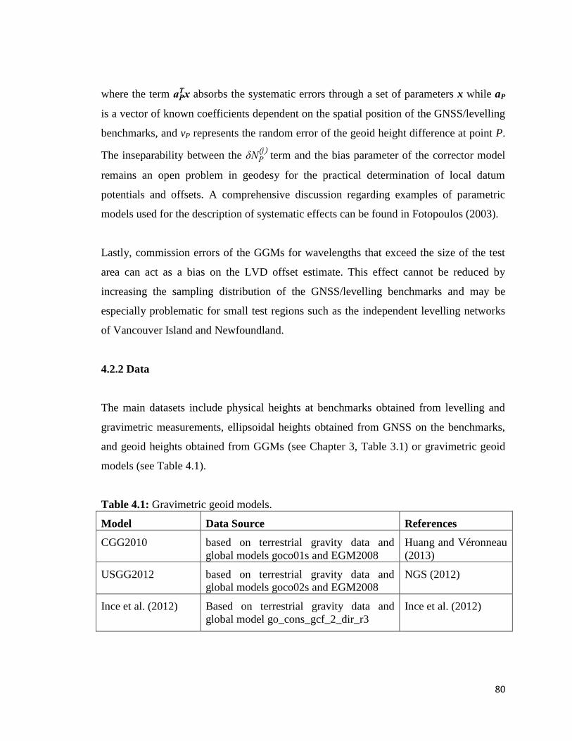
80
where the term absorbs the systematic errors through a set of parameters x while aP
is a vector of known coefficients dependent on the spatial position of the GNSS/levelling
benchmarks, and vP represents the random error of the geoid height difference at point P.
The inseparability between the δN term and the bias parameter of the corrector model
remains an open problem in geodesy for the practical determination of local datum
potentials and offsets. A comprehensive discussion regarding examples of parametric
models used for the description of systematic effects can be found in Fotopoulos (2003).
Lastly, commission errors of the GGMs for wavelengths that exceed the size of the test
area can act as a bias on the LVD offset estimate. This effect cannot be reduced by
increasing the sampling distribution of the GNSS/levelling benchmarks and may be
especially problematic for small test regions such as the independent levelling networks
of Vancouver Island and Newfoundland.
4.2.2 Data
The main datasets include physical heights at benchmarks obtained from levelling and
gravimetric measurements, ellipsoidal heights obtained from GNSS on the benchmarks,
and geoid heights obtained from GGMs (see Chapter 3, Table 3.1) or gravimetric geoid
models (see Table 4.1).
Table 4.1: Gravimetric geoid models.
Model Data Source References
CGG2010 based on terrestrial gravity data and
global models goco01s and EGM2008
Huang and Véronneau
(2013)
USGG2012 based on terrestrial gravity data and
global models goco02s and EGM2008
NGS (2012)
Ince et al. (2012) Based on terrestrial gravity data and
global model go_cons_gcf_2_dir_r3
Ince et al. (2012)
81
4.2.3 GNSS/Levelling Benchmark Distribution
Two subsets of GNSS/levelling benchmarks are used in Canada while the 18,399
GNSS/levelling benchmarks presented in Chapter 3 for GOCE model evaluation (see
Figure 3.5) are utilized for the computation of LVD offsets for the NAVD88 datum in the
U.S.A.
The first dataset in Canada refers to 308 benchmarks, where the original ellipsoidal
heights and coordinates were given in ITRF2005 (Altamimi et al. 2007) epoch 2006.0
and come from the adjustment of the GPS SuperNet network in Canada (Craymer and
Lapelle 1997). These have been updated to ITRF2008 epoch 2008.0 using software
developed by the U.S.A. National Geodetic Survey (available at
http://www.ngs.noaa.gov/TOOLS/Htdp/Htdp.shtml), taking into account the effect of
post-glacial rebound using the velocities from the Argus and Peltier (2010) GEODVEL1b
GPS solution. This correction was applied using a 2-D linear interpolation and with the
assumption that the acceleration of the vertical motion is zero. These benchmarks have
physical heights obtained from levelling that refer to CGVD28, NAVD88, and the Nov07
vertical datums (see Figure 4.3).
The next dataset refers to levelling data given with respect to the Nov07 vertical datum.
There are three main regions: Canadian Mainland (CML), Newfoundland (NFD), and
Vancouver Island (VAN).
For the Canadian mainland (see Figure 4.4), the relief of the terrain ranges from mean sea
level to 500 m for eastern and most of central Canada while the topography becomes
quite rugged for the western portion of the country where the elevation ranges from 500
m to 3000 m, reaching a maximum of 5000 m or more in a few selected areas (Natural
Resources Canada 2007).

82
Figure 4.3: Distribution of 308 GNSS/levelling benchmarks common in Nov07,
CGVD28, and NAVD88 vertical datums.
Figure 4.4: Distribution of 1,315 GNSS/levelling benchmarks in the Nov07 vertical
datum for the Canadian mainland (CML).
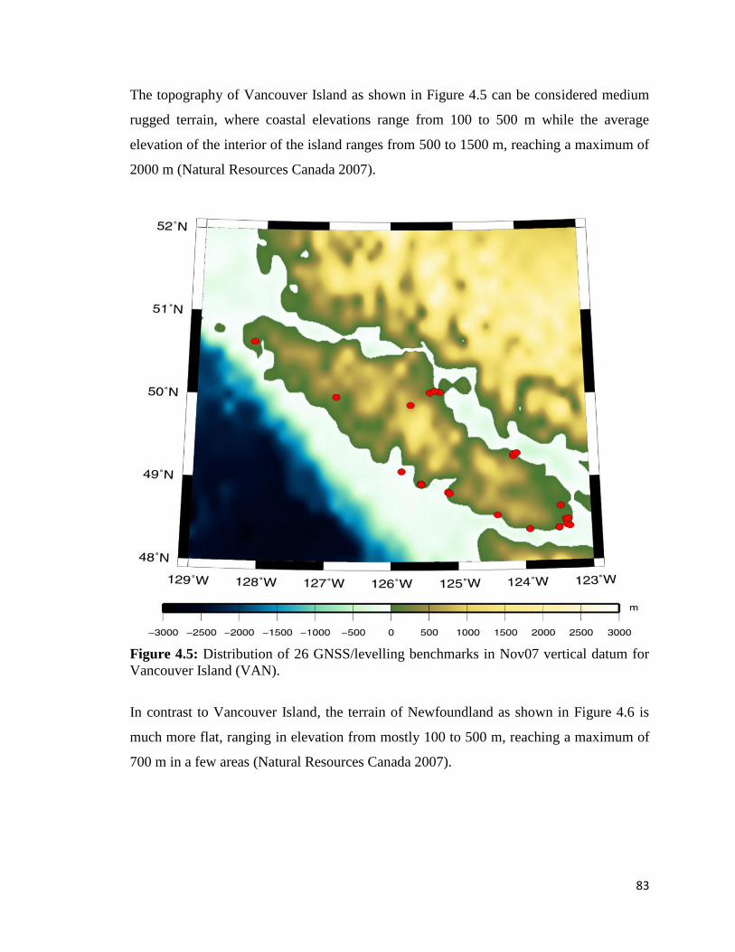
83
The topography of Vancouver Island as shown in Figure 4.5 can be considered medium
rugged terrain, where coastal elevations range from 100 to 500 m while the average
elevation of the interior of the island ranges from 500 to 1500 m, reaching a maximum of
2000 m (Natural Resources Canada 2007).
Figure 4.5: Distribution of 26 GNSS/levelling benchmarks in Nov07 vertical datum for
Vancouver Island (VAN).
In contrast to Vancouver Island, the terrain of Newfoundland as shown in Figure 4.6 is
much more flat, ranging in elevation from mostly 100 to 500 m, reaching a maximum of
700 m in a few areas (Natural Resources Canada 2007).
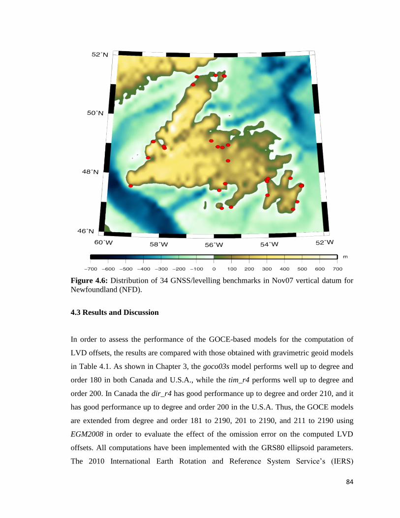
84
Figure 4.6: Distribution of 34 GNSS/levelling benchmarks in Nov07 vertical datum for
Newfoundland (NFD).
4.3 Results and Discussion
In order to assess the performance of the GOCE-based models for the computation of
LVD offsets, the results are compared with those obtained with gravimetric geoid models
in Table 4.1. As shown in Chapter 3, the goco03s model performs well up to degree and
order 180 in both Canada and U.S.A., while the tim_r4 performs well up to degree and
order 200. In Canada the dir_r4 has good performance up to degree and order 210, and it
has good performance up to degree and order 200 in the U.S.A. Thus, the GOCE models
are extended from degree and order 181 to 2190, 201 to 2190, and 211 to 2190 using
EGM2008 in order to evaluate the effect of the omission error on the computed LVD
offsets. All computations have been implemented with the GRS80 ellipsoid parameters.
The 2010 International Earth Rotation and Reference System Service’s (IERS)

85
conventional value of 62636856.00 m2/s
2 (Petit and Luzum 2010) was used for W0
defining the global equipotential surface. The height data are all in a tide-free system.
4.3.1 Estimating CGVD28, NAVD88, and Nov07 LVD Offsets in Canada using 308
GNSS/Levelling Benchmarks
Table 4.2 presents the LVD offsets of Nov07, NAVD88, and CGVD28 for the data set of
308 GNSS/levelling benchmarks distributed mainly along the southern region of Canada
(see Figure 4.3). The results are shown in terms of the potential difference between the
reference conventional surface and the local datum (i.e., δW(j)
) and the offset of the LVD
(i.e., δN(j)
). For the least-squares evaluation of Eq. (4.12), a unit weight matrix has been
used, assuming a constant and uncorrelated noise in the known heights at all data points;
the error estimates shown in the tables indicate a formal statistical accuracy only. The
main objective of this section is to estimate the effect of the GOCE model omission error
on LVD offset estimations, and as such the effects of systematic errors have not been
taken into account for the numerical computations presented herein.
The effect of the GOCE omission error is quite significant in Canada when computing
LVD offsets. For example, from Table 4.2 , the Nov07 offset computed with
goco03s+EGM2008 is -44.8 cm and the offset computed with tim_r4+EGM2008 is -44.9
cm while the GOCE only models yield -58.2 cm and -53.3 cm, respectively. Thus, the
effect of the GOCE GGM omission error on the LVD offsets can be quantified as 13 cm
for the third generation GOCE GGM truncated at degree and order 180, and 8 cm for the
fourth generation GOCE GGMs truncated at degree and order 200 and 210. Based on the
results from Table 4.2, it can be seen that both dir_r4 and tim_r4 perform very similarly
when the models are truncated at degree and order 200 and 210, respectively; the
difference between the evaluated LVD offsets is less than 1 cm. The similar performance
is expected as both models use the same 27 months of GOCE observations and similar
data pre-processing (Pail et al., 2011). Likewise, the itg-grace2010s omission error
affects the computed LVD offsets by 13 cm.

86
It is expected that the results obtained with CGG2010, EGM2008, GRACE+EGM2008,
and the GOCE+EGM2008 models will be similar as the same high quality gravity data
are utilized by all three models. For example, the Nov07 offset evaluated with EGM2008
is -44.8 cm and with CGG2010 it is -45.2 cm. It can be seen that CGG2010 yields a 13
cm difference between the offsets computed with goco03s, and an 8 cm difference
between the offset computed with tim_r4, which is similar to the omission error
approximated by EGM2008. However, a 15 cm effect is observed when itg-grace2010s is
used. Based on the smaller offset difference, it can be concluded that tim_r4 or dir_r4
should be preferred to itg-grace2010s for the LVD offset computations.
It can also be observed from Table 4.2 that the formal standard deviations of the
estimated LVD offsets decrease when using models that incorporate the higher frequency
information of the gravity field. For example, the standard deviation of the Nov07 offset
using goco03s is 2.1 cm while it reduces to 0.7 cm in the goco03s+EGM2008 case. This
is because the geoid heights computed with the GOCE+EGM2008 models are more
spectrally consistent with the GNSS-levelling geoid heights than the geoid heights
computed with the truncated GOCE models of degree 180. In general, it can also be
observed that the standard deviations of the estimated NAVD88 (e.g., 2.2 cm) and
CGVD28 (e.g., 1.7 cm) offsets are larger than the standard deviation of the Nov07 offset
(e.g., 0.7 cm), which can be explained by the differences in the existing systematic errors
and local datum distortions in NAVD88 and CGVD28 described in Chapter 2 Section
2.5.
4.3.2 Estimating Nov07 LVD Offsets for CML, VAN, and NFD Networks
Table 4.3 shows the Nov07 offset computed with the CGG2010, Ince et al. (2012),
goco03s+EGM2008, and tim_r4+EGM2008 models, as well as the goco03s and tim_r4
models. The LVD offsets for VAN and NFD are evaluated for a local level surface that is
different from that of the Nov07 CML network.
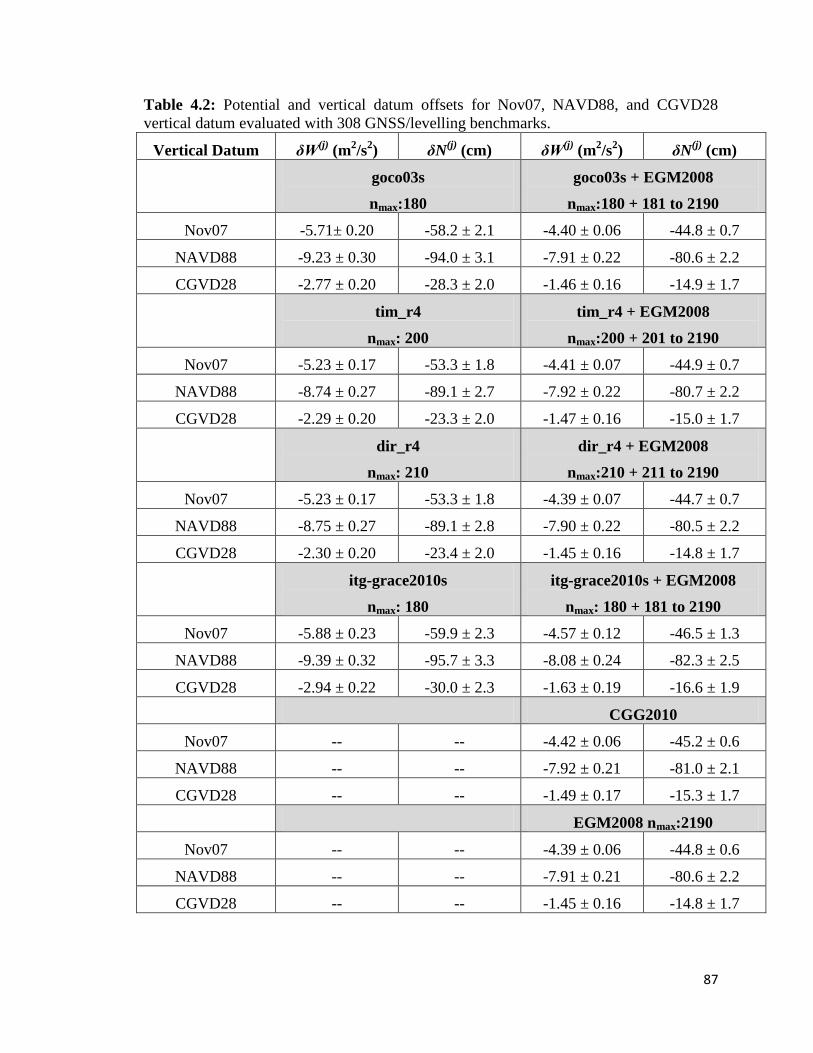
87
Table 4.2: Potential and vertical datum offsets for Nov07, NAVD88, and CGVD28
vertical datum evaluated with 308 GNSS/levelling benchmarks.
Vertical Datum δW(j)
(m2/s
2) δN
(j) (cm) δW
(j) (m
2/s
2) δN
(j) (cm)
goco03s
nmax:180
goco03s + EGM2008
nmax:180 + 181 to 2190
Nov07 -5.71± 0.20 -58.2 ± 2.1 -4.40 ± 0.06 -44.8 ± 0.7
NAVD88 -9.23 ± 0.30 -94.0 ± 3.1 -7.91 ± 0.22 -80.6 ± 2.2
CGVD28 -2.77 ± 0.20 -28.3 ± 2.0 -1.46 ± 0.16 -14.9 ± 1.7
tim_r4
nmax: 200
tim_r4 + EGM2008
nmax:200 + 201 to 2190
Nov07 -5.23 ± 0.17 -53.3 ± 1.8 -4.41 ± 0.07 -44.9 ± 0.7
NAVD88 -8.74 ± 0.27 -89.1 ± 2.7 -7.92 ± 0.22 -80.7 ± 2.2
CGVD28 -2.29 ± 0.20 -23.3 ± 2.0 -1.47 ± 0.16 -15.0 ± 1.7
dir_r4
nmax: 210
dir_r4 + EGM2008
nmax:210 + 211 to 2190
Nov07 -5.23 ± 0.17 -53.3 ± 1.8 -4.39 ± 0.07 -44.7 ± 0.7
NAVD88 -8.75 ± 0.27 -89.1 ± 2.8 -7.90 ± 0.22 -80.5 ± 2.2
CGVD28 -2.30 ± 0.20 -23.4 ± 2.0 -1.45 ± 0.16 -14.8 ± 1.7
itg-grace2010s
nmax: 180
itg-grace2010s + EGM2008
nmax: 180 + 181 to 2190
Nov07 -5.88 ± 0.23 -59.9 ± 2.3 -4.57 ± 0.12 -46.5 ± 1.3
NAVD88 -9.39 ± 0.32 -95.7 ± 3.3 -8.08 ± 0.24 -82.3 ± 2.5
CGVD28 -2.94 ± 0.22 -30.0 ± 2.3 -1.63 ± 0.19 -16.6 ± 1.9
CGG2010
Nov07 -- -- -4.42 ± 0.06 -45.2 ± 0.6
NAVD88 -- -- -7.92 ± 0.21 -81.0 ± 2.1
CGVD28 -- -- -1.49 ± 0.17 -15.3 ± 1.7
EGM2008 nmax:2190
Nov07 -- -- -4.39 ± 0.06 -44.8 ± 0.6
NAVD88 -- -- -7.91 ± 0.21 -80.6 ± 2.2
CGVD28 -- -- -1.45 ± 0.16 -14.8 ± 1.7
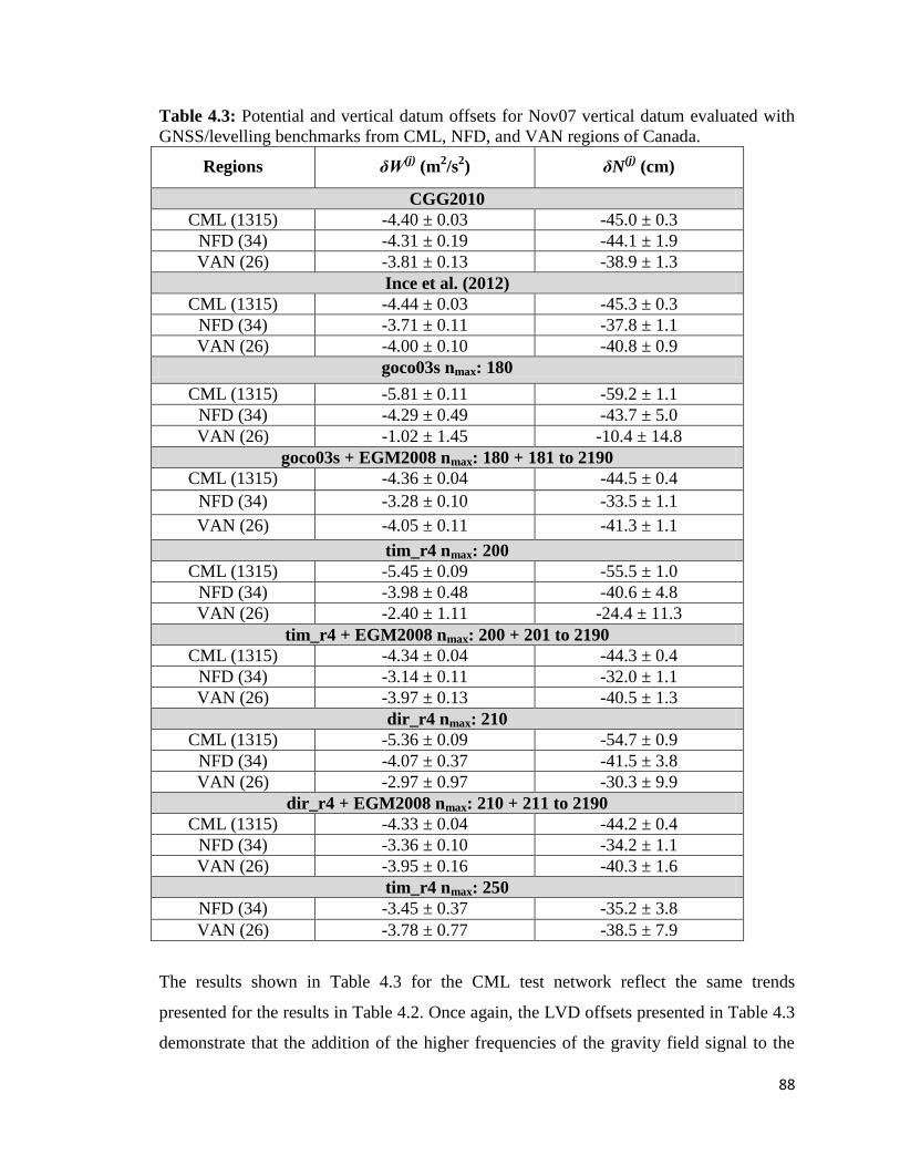
88
Table 4.3: Potential and vertical datum offsets for Nov07 vertical datum evaluated with
GNSS/levelling benchmarks from CML, NFD, and VAN regions of Canada.
Regions δW(j)
(m2/s
2) δN
(j) (cm)
CGG2010
CML (1315) -4.40 ± 0.03 -45.0 ± 0.3
NFD (34) -4.31 ± 0.19 -44.1 ± 1.9
VAN (26) -3.81 ± 0.13 -38.9 ± 1.3
Ince et al. (2012)
CML (1315) -4.44 ± 0.03 -45.3 ± 0.3
NFD (34) -3.71 ± 0.11 -37.8 ± 1.1
VAN (26) -4.00 ± 0.10 -40.8 ± 0.9
goco03s nmax: 180
CML (1315) -5.81 ± 0.11 -59.2 ± 1.1
NFD (34) -4.29 ± 0.49 -43.7 ± 5.0
VAN (26) -1.02 ± 1.45 -10.4 ± 14.8
goco03s + EGM2008 nmax: 180 + 181 to 2190
CML (1315) -4.36 ± 0.04 -44.5 ± 0.4
NFD (34) -3.28 ± 0.10 -33.5 ± 1.1
VAN (26) -4.05 ± 0.11 -41.3 ± 1.1
tim_r4 nmax: 200
CML (1315) -5.45 ± 0.09 -55.5 ± 1.0
NFD (34) -3.98 ± 0.48 -40.6 ± 4.8
VAN (26) -2.40 ± 1.11 -24.4 ± 11.3
tim_r4 + EGM2008 nmax: 200 + 201 to 2190
CML (1315) -4.34 ± 0.04 -44.3 ± 0.4
NFD (34) -3.14 ± 0.11 -32.0 ± 1.1
VAN (26) -3.97 ± 0.13 -40.5 ± 1.3
dir_r4 nmax: 210
CML (1315) -5.36 ± 0.09 -54.7 ± 0.9
NFD (34) -4.07 ± 0.37 -41.5 ± 3.8
VAN (26) -2.97 ± 0.97 -30.3 ± 9.9
dir_r4 + EGM2008 nmax: 210 + 211 to 2190
CML (1315) -4.33 ± 0.04 -44.2 ± 0.4
NFD (34) -3.36 ± 0.10 -34.2 ± 1.1
VAN (26) -3.95 ± 0.16 -40.3 ± 1.6
tim_r4 nmax: 250
NFD (34) -3.45 ± 0.37 -35.2 ± 3.8
VAN (26) -3.78 ± 0.77 -38.5 ± 7.9
The results shown in Table 4.3 for the CML test network reflect the same trends
presented for the results in Table 4.2. Once again, the LVD offsets presented in Table 4.3
demonstrate that the addition of the higher frequencies of the gravity field signal to the

89
GOCE GGMs is an important factor for the accurate determination of the LVD offsets in
Canada. Therefore, it is recommended that a rigorously combined GOCE GGM and local
gravity and terrain data should be used when using GOCE-based GGMs for the
evaluation of LVD offsets in Canada.
The results from Table 4.3 emphasize the fact that simply increasing the number of
GNSS/levelling benchmarks will not necessarily reduce the effect of the GOCE omission
error on the LVD offsets. For example, the offset for the CML network computed with
1,315 benchmarks and the tim_r4 model is -55.5 cm while it was -53.3 cm when
evaluated with 308 benchmarks. In this case, increasing the number of benchmarks has
actually increased the effect of the GOCE omission error by 2 cm. This increase in the
effect of the GOCE omission error can be explained by the fact that a portion of the
newly added points are located in the rugged terrain of western Canada; as well the
distribution of the benchmarks in the CML network is not necessarily improved with
respect to the 308 benchmark case of the previous section (see Figures 4.3 and 4.4). Thus,
another factor that will affect the LVD offset estimate, in addition to the density of the
benchmarks, is the configuration of the GNSS-levelling network.
For the offsets estimated on the two islands (i.e., VAN and NFD) the effects of the
limited geographical coverage and sparse and irregular distribution of the GNSS/levelling
benchmarks can be observed from the results in Table 4.3. For example, the offset
evaluated for VAN using goco03s only is -10.4 ± 14.8 cm when compared to -38.9 ± 1.3
cm with CGG2010 and -40.8 ± 0.9 cm with the Ince et al. (2012) model. Using the 3-
sigma test, it can be seen that the offset computed with goco03s (as well as the tim_r4
model) yields a statistically insignificant LVD offset for Vancouver Island as the
estimated LVD offset is smaller than three times its formal error. This insignificant result
can be further explained by the effect of the GOCE omission error on the LVD offset of
Vancouver Island, which is expected to be quite significant due to its rugged terrain (see
Figure 4.5). In other words, neither the goco03s nor the tim_r4 model truncated at degree
and order 180 and 200, respectively, sufficiently models the geoid signal on Vancouver
Island. On the other hand, it can be seen from Table 4.3 that when the offset is evaluated
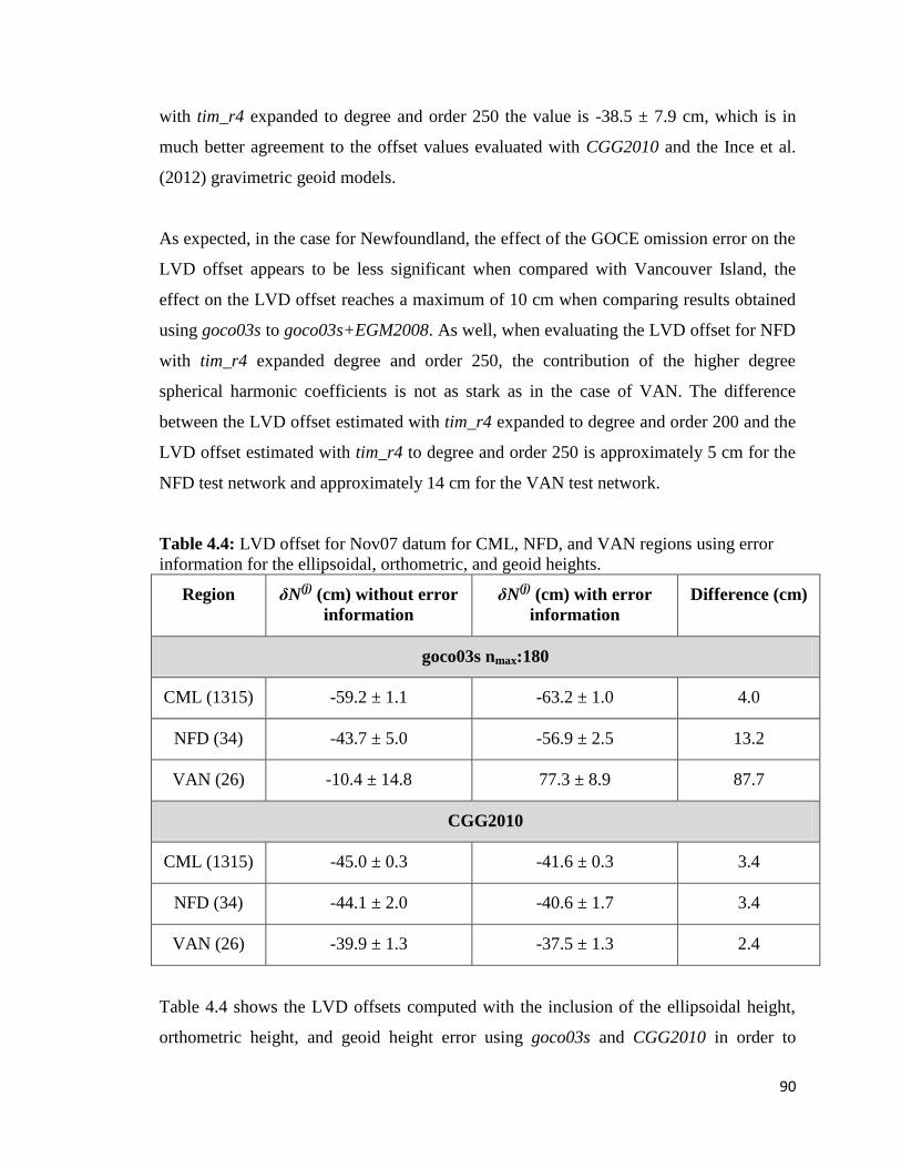
90
with tim_r4 expanded to degree and order 250 the value is -38.5 ± 7.9 cm, which is in
much better agreement to the offset values evaluated with CGG2010 and the Ince et al.
(2012) gravimetric geoid models.
As expected, in the case for Newfoundland, the effect of the GOCE omission error on the
LVD offset appears to be less significant when compared with Vancouver Island, the
effect on the LVD offset reaches a maximum of 10 cm when comparing results obtained
using goco03s to goco03s+EGM2008. As well, when evaluating the LVD offset for NFD
with tim_r4 expanded degree and order 250, the contribution of the higher degree
spherical harmonic coefficients is not as stark as in the case of VAN. The difference
between the LVD offset estimated with tim_r4 expanded to degree and order 200 and the
LVD offset estimated with tim_r4 to degree and order 250 is approximately 5 cm for the
NFD test network and approximately 14 cm for the VAN test network.
Table 4.4: LVD offset for Nov07 datum for CML, NFD, and VAN regions using error
information for the ellipsoidal, orthometric, and geoid heights.
Region δN(j)
(cm) without error
information
δN(j)
(cm) with error
information
Difference (cm)
goco03s nmax:180
CML (1315) -59.2 ± 1.1 -63.2 ± 1.0 4.0
NFD (34) -43.7 ± 5.0 -56.9 ± 2.5 13.2
VAN (26) -10.4 ± 14.8 77.3 ± 8.9 87.7
CGG2010
CML (1315) -45.0 ± 0.3 -41.6 ± 0.3 3.4
NFD (34) -44.1 ± 2.0 -40.6 ± 1.7 3.4
VAN (26) -39.9 ± 1.3 -37.5 ± 1.3 2.4
Table 4.4 shows the LVD offsets computed with the inclusion of the ellipsoidal height,
orthometric height, and geoid height error using goco03s and CGG2010 in order to
91
evaluate the effect of including accuracy information on the LVD offset estimations. The
variances of the spherical harmonic coefficients were used when propagating the
commission errors from the GOCE model to the geoid heights. The average error for the
geoid heights obtained from goco03s is 3.4 cm. The error estimates for the ellipsoidal
heights, orthometric heights, and geoid heights obtained from the CGG2010 model were
provided by GSD. For the VAN test network the mean ellipsoidal height error is
approximately 1 cm, the mean orthometric height error is approximately 2 cm, and the
average error for the geoid heights obtained from the CGG2010 model is 5 cm. For the
NFD test network, the average ellipsoidal and orthometric height errors are the same as
for the VAN test network while the average geoid height error from the CGG2010 model
is 2 cm. Lastly, for the CML test network the mean ellipsoidal height error is 1 cm, the
mean orthometric height error is 6 cm, and the mean geoid height error obtained from the
CGG2010 model is 3 cm.
Based on the results presented in Table 4.4, a 4 cm difference can be observed in the
LVD offset computed using GOCE commission error information up to degree and order
180, in combination with the error estimates for the ellipsoidal and levelling heights,
when compared to the LVD offset estimated without any error information for the CML
region. This effect is more pronounced for Newfoundland, where the difference is 13 cm.
One of the reasons contributing to this difference can be explained by the fact that the
geographical coverage of the NFD network is much smaller when compared to the
geographic coverage of the CML network, and therefore it is more likely to be affected
by the commission errors of the GGM wavelengths that exceed the size of the test area.
The large difference of almost 88 cm for Vancouver Island may be due to the uncertain
reliability of the control data and their errors on Vancouver Island, in addition to the fact
that utilizing only the goco03s model extended to degree and order 180 for the VAN test
network yields statistically insignificant results. Moreover, using only the variances of
the spherical harmonic coefficients may also have an effect as the inclusion of a full
variance co-variance matrix may yield different results. Thus, for each of the islands, the
computed potential and offset for the Nov07 datum demonstrate that the GGM
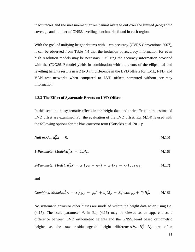
92
inaccuracies and the measurement errors cannot average out over the limited geographic
coverage and number of GNSS/levelling benchmarks found in each region.
With the goal of unifying height datums with 1 cm accuracy (CVRS Conventions 2007),
it can be observed from Table 4.4 that the inclusion of accuracy information for even
high resolution models may be necessary. Utilizing the accuracy information provided
with the CGG2010 model yields in combination with the errors of the ellipsoidal and
levelling heights results in a 2 to 3 cm difference in the LVD offsets for CML, NFD, and
VAN test networks when compared to LVD offsets computed without accuracy
information.
4.3.3 The Effect of Systematic Errors on LVD Offsets
In this section, the systematic effects in the height data and their effect on the estimated
LVD offset are examined. For the evaluation of the LVD offset, Eq. (4.14) is used with
the following options for the bias corrector term (Kotsakis et al. 2011):
Null model: , (4.15)
1-Parameter Model:
, (4.16)
2-Parameter Model: (4.17)
and
Combined Model:
. (4.18)
No systematic errors or other biases are modeled within the height data when using Eq.
(4.15). The scale parameter δs in Eq. (4.16) may be viewed as an apparent scale
difference between LVD orthometric heights and the GNSS/geoid based orthometric
heights as the raw residuals/geoid height differences h -
- N are often

93
topographically correlated. The application of the systematic model shown in Eq. (4.16)
will only be successful in a test network that has a significant height variability so that the
offset parameter δN
and the scale parameter δs can be sufficiently separated through the
least-squares estimation (Kotsakis et al. 2011) of Eq. (4.14). In general, if one expects to
obtain realistic estimates of the LVD offset, the vertical offset term should not be
strongly correlated with the adopted bias corrector term model. Thus the bias corrector
term model should not contain any components that remain constant or almost constant
over the test network. As discussed in the previous section, it should be noted that for test
networks with limited geographic coverage, the long-wavelength geoid errors will
contaminate the least-squares estimate of the LVD offset, thus for such networks it is
necessary to include the GGM commission errors for spatial wavelengths the exceed the
size of the test area when utilizing bias corrector term models to estimate the effect of
systematic errors on LVD offsets. For the model in Eq. (4.17), φ is the latitude of the
GNSS/levelling benchmark and λ is the longitude; the overall tilt consists of a N-S
component x1, and a W-E component x2 with respect to the centroid of the test network
(φ , λ ). The combined model shown by Eq. (4.18) consists of a combination of the 1-
parameter and the 2-parameter model.
The geoid height differences are plotted in Figures 4.7 to 4.10 in order to show the spatial
tilts present in the respective GNSS/levelling networks while the distribution of the
orthometric heights of the Canadian Nov07, NAVD88, CGVD28, and the U.S.A.
NAVDD88 test networks are shown in Figures 4.11 to 4.14, respectively. Figures 4.7 to
4.9 show that for the Canadian Nov07, NAVD88, and CGVD28 test networks there exists
a significant east-west tilt, and a less significant north-south tilt while for the U.S.A.
NAVD88 test network, shown in Figure 4.10, there is both a significant east-west and
north-south tilt.
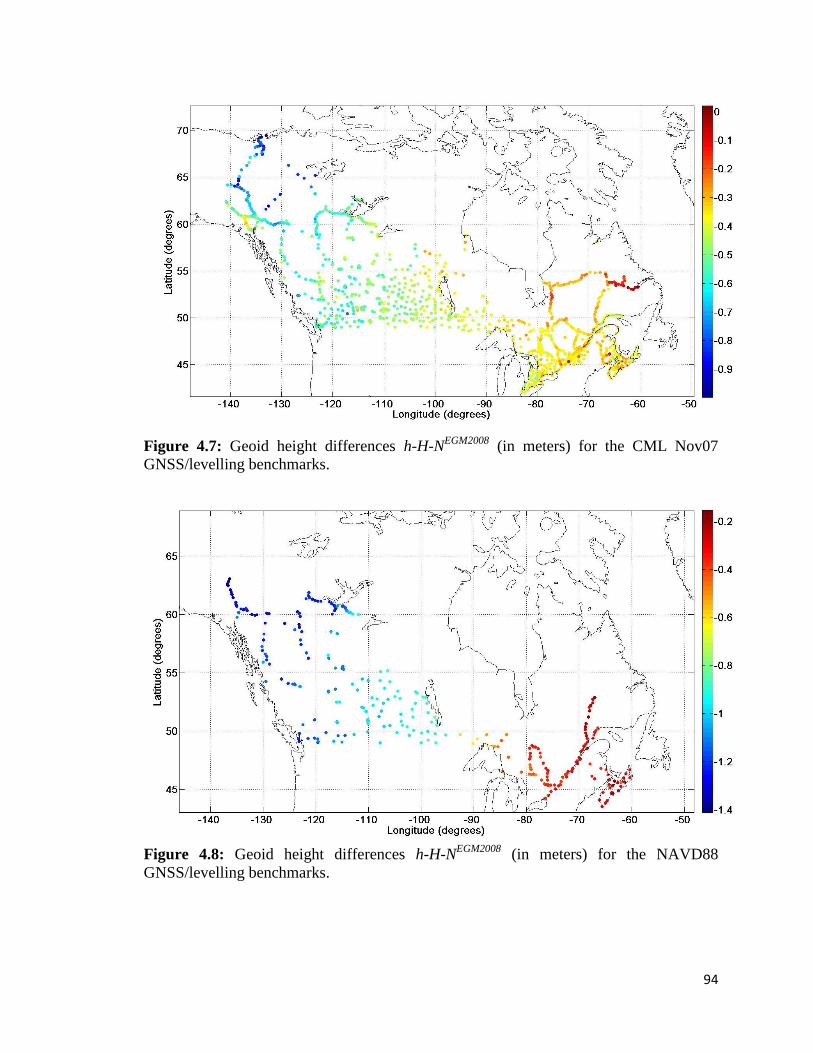
94
Figure 4.7: Geoid height differences h-H-N
EGM2008 (in meters) for the CML Nov07
GNSS/levelling benchmarks.
Figure 4.8: Geoid height differences h-H-N
EGM2008 (in meters) for the NAVD88
GNSS/levelling benchmarks.
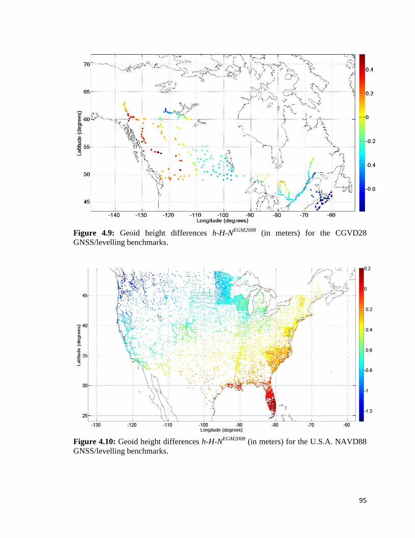
95
Figure 4.9: Geoid height differences h-H-N
EGM2008 (in meters) for the CGVD28
GNSS/levelling benchmarks.
Figure 4.10: Geoid height differences h-H-N
EGM2008 (in meters) for the U.S.A. NAVD88
GNSS/levelling benchmarks.
96
Figure 4.11: Distribution of H (m) in Nov07 GNSS/levelling network (1,315
benchmarks).
Figure 4.12: Distribution of H (m) in NAVD88 GNSS/levelling network (308
benchmarks).
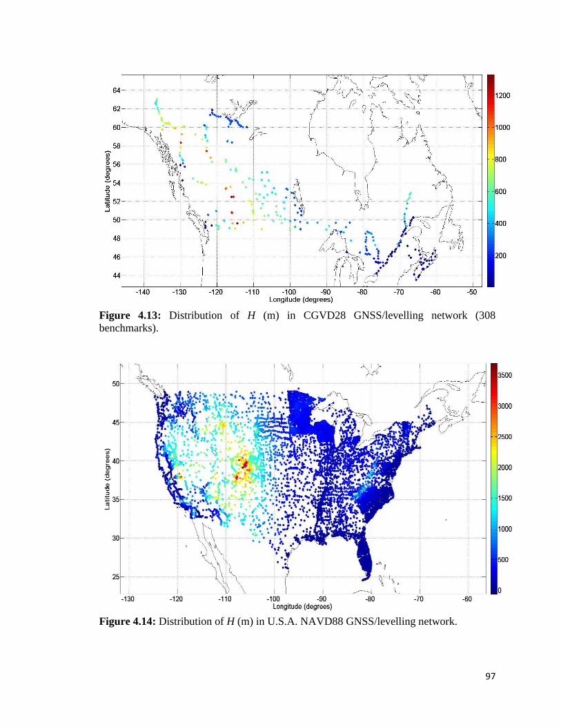
97
Figure 4.13: Distribution of H (m) in CGVD28 GNSS/levelling network (308
benchmarks).
Figure 4.14: Distribution of H (m) in U.S.A. NAVD88 GNSS/levelling network.
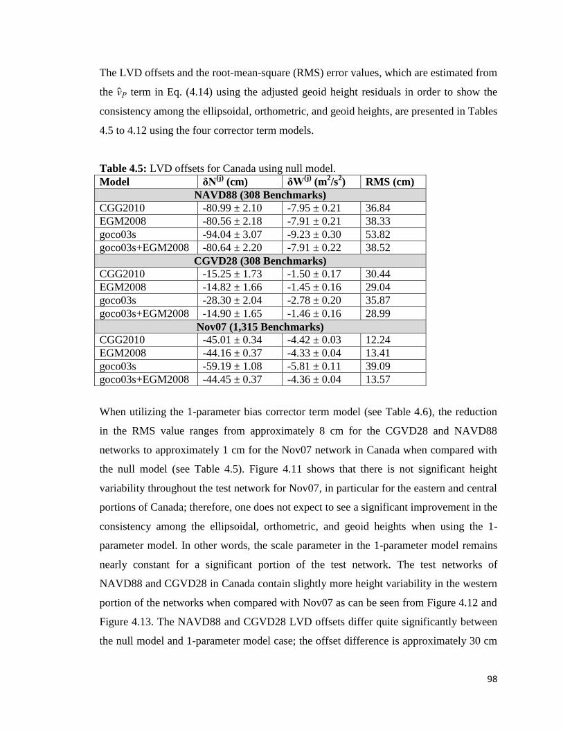
98
The LVD offsets and the root-mean-square (RMS) error values, which are estimated from
the term in Eq. (4.14) using the adjusted geoid height residuals in order to show the
consistency among the ellipsoidal, orthometric, and geoid heights, are presented in Tables
4.5 to 4.12 using the four corrector term models.
Table 4.5: LVD offsets for Canada using null model.
Model δN(j)
(cm) δW(j)
(m2/s
2) RMS (cm)
NAVD88 (308 Benchmarks)
CGG2010 -80.99 ± 2.10 -7.95 ± 0.21 36.84
EGM2008 -80.56 ± 2.18 -7.91 ± 0.21 38.33
goco03s -94.04 ± 3.07 -9.23 ± 0.30 53.82
goco03s+EGM2008 -80.64 ± 2.20 -7.91 ± 0.22 38.52
CGVD28 (308 Benchmarks)
CGG2010 -15.25 ± 1.73 -1.50 ± 0.17 30.44
EGM2008 -14.82 ± 1.66 -1.45 ± 0.16 29.04
goco03s -28.30 ± 2.04 -2.78 ± 0.20 35.87
goco03s+EGM2008 -14.90 ± 1.65 -1.46 ± 0.16 28.99
Nov07 (1,315 Benchmarks)
CGG2010 -45.01 ± 0.34 -4.42 ± 0.03 12.24
EGM2008 -44.16 ± 0.37 -4.33 ± 0.04 13.41
goco03s -59.19 ± 1.08 -5.81 ± 0.11 39.09
goco03s+EGM2008 -44.45 ± 0.37 -4.36 ± 0.04 13.57
When utilizing the 1-parameter bias corrector term model (see Table 4.6), the reduction
in the RMS value ranges from approximately 8 cm for the CGVD28 and NAVD88
networks to approximately 1 cm for the Nov07 network in Canada when compared with
the null model (see Table 4.5). Figure 4.11 shows that there is not significant height
variability throughout the test network for Nov07, in particular for the eastern and central
portions of Canada; therefore, one does not expect to see a significant improvement in the
consistency among the ellipsoidal, orthometric, and geoid heights when using the 1-
parameter model. In other words, the scale parameter in the 1-parameter model remains
nearly constant for a significant portion of the test network. The test networks of
NAVD88 and CGVD28 in Canada contain slightly more height variability in the western
portion of the networks when compared with Nov07 as can be seen from Figure 4.12 and
Figure 4.13. The NAVD88 and CGVD28 LVD offsets differ quite significantly between
the null model and 1-parameter model case; the offset difference is approximately 30 cm
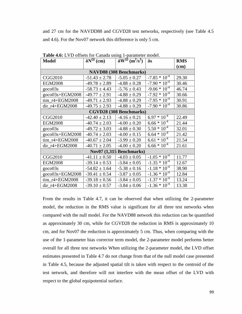
99
and 27 cm for the NAVDD88 and CGVD28 test networks, respectively (see Table 4.5
and 4.6). For the Nov07 network this difference is only 5 cm.
Table 4.6: LVD offsets for Canada using 1-parameter model.
Model δN(j)
(cm) δW(j)
(m2/s
2) δs RMS
(cm)
NAVD88 (308 Benchmarks)
CGG2010 -51.43 ± 2.78 -5.05 ± 0.27 -7.85 * 10-4
29.30
EGM2008 -49.78 ± 2.89 -4.88 ± 0.28 -7.90 * 10-4
30.46
goco03s -58.73 ± 4.43 -5.76 ± 0.43 -9.06 * 10-4
46.74
goco03s+EGM2008 -49.77 ± 2.91 -4.88 ± 0.29 -7.92 * 10-4
30.66
tim_r4+EGM2008 -49.71 ± 2.93 -4.88 ± 0.29 -7.95 * 10-4
30.91
dir_r4+EGM2008 -49.75 ± 2.93 -4.88 ± 0.29 -7.90 * 10-4
30.86
CGVD28 (308 Benchmarks)
CGG2010 -42.40 ± 2.13 -4.16 ± 0.21 6.97 * 10-4
22.49
EGM2008 -40.74 ± 2.03 -4.00 ± 0.20 6.66 * 10-4
21.44
goco03s -49.72 ± 3.03 -4.88 ± 0.30 5.50 * 10-4
32.01
goco03s+EGM2008 -40.74 ± 2.03 -4.00 ± 0.15 6.64 * 10-4
21.42
tim_r4+EGM2008 -40.67 ± 2.04 -3.99 ± 0.20 6.61 * 10-4
21.54
dir_r4+EGM2008 -40.71 ± 2.05 -4.00 ± 0.20 6.66 * 10-4
21.61
Nov07 (1,315 Benchmarks)
CGG2010 -41.11 ± 0.50 -4.03 ± 0.05 -1.05 * 10-4
11.77
EGM2008 -39.14 ± 0.53 -3.84 ± 0.05 -1.35 * 10-4
12.67
goco03s -54.82 ± 1.64 -5.38 ± 0.16 -1.18 * 10-4
38.90
goco03s+EGM2008 -39.41 ± 0.54 -3.87 ± 0.05 -1.36 * 10-4
12.84
tim_r4+EGM2008 -39.18 ± 0.56 -3.84 ± 0.05 -1.37 * 10-4
13.24
dir_r4+EGM2008 -39.10 ± 0.57 -3.84 ± 0.06 -1.36 * 10-4
13.38
From the results in Table 4.7, it can be observed that when utilizing the 2-parameter
model, the reduction in the RMS value is significant for all three test networks when
compared with the null model. For the NAVD88 network this reduction can be quantified
as approximately 30 cm, while for CGVD28 the reduction in RMS is approximately 10
cm, and for Nov07 the reduction is approximately 5 cm. Thus, when comparing with the
use of the 1-parameter bias corrector term model, the 2-parameter model performs better
overall for all three test networks When utilizing the 2-parameter model, the LVD offset
estimates presented in Table 4.7 do not change from that of the null model case presented
in Table 4.5, because the adjusted spatial tilt is taken with respect to the centroid of the
test network, and therefore will not interfere with the mean offset of the LVD with
respect to the global equipotential surface.

100
Table 4.7: LVD offsets for Canada using 2-parameter model.
Model δNj (cm) δW
j (m
2/s
2) NS
(m/deg)
WE
(m/deg)
RMS
(cm)
NAVD88 (308 Benchmarks)
CGG2010 -80.99 ± 2.10 -7.95 ± 0.21 -0.004 0.023 8.15
EGM2008 -80.56 ± 2.18 -7.91 ± 0.21 -0.003 0.025 8.12
goco03s -94.04 ± 3.07 -9.23 ± 0.30 0.025 0.038 30.01
goco03s+EGM2008 -80.64 ± 2.20 -7.91 ± 0.22 -0.002 0.025 8.29
tim_r4+EGM2008 -80.70 ± 0.48 -7.92 ± 0.05 -0.003 0.025 8.42
dir_r4+EGM2008 -80.53 ± 0.49 -7.90 ± 0.05 -0.003 0.025 8.56
CGVD28 (308 Benchmarks)
CGG2010 -15.25 ± 1.13 -1.50 ± 0.11 -0.014 -0.020 19.80
EGM2008 -14.82 ± 1.11 -1.45 ± 0.11 -0.012 -0.018 19.50
goco03s -28.30 ± 1.87 -2.78 ± 0.18 0.015 -0.005 32.41
goco03s+EGM2008 -14.90 ± 1.12 -1.46 ± 0.11 -0.012 -0.018 19.63
tim_r4+EGM2008 -14.96 ± 1.14 -1.47 ± 0.11 -0.013 -0.018 19.87
dir_r4+EGM2008 -14.79 ± 1.14 -1.45 ± 0.11 -0.012 -0.018 19.93
Nov07 (1,315 Benchmarks)
CGG2010 -45.01 ± 0.23 -4.42 ± 0.02 -0.003 0.005 8.30
EGM2008 -44.16 ± 0.23 -4.33 ± 0.02 -0.002 0.007 8.19
goco03s -59.19 ± 0.96 -5.81 ± 0.09 0.010 0.015 34.73
goco03s+EGM2008 -44.45 ± 0.22 -4.36 ± 0.02 -0.001 0.007 8.11
tim_r4+EGM2008 -44.27 ± 0.23 -4.34 ± 0.02 -0.002 0.007 8.46
dir_r4+EGM2008 -44.17 ± 0.24 -4.33 ± 0.02 -0.002 0.007 8.67
There is not a significant decrease in the RMS values when utilizing the combined model
with respect to the 2-parameter model. From Table 4.8 it can be seen that the reduction is
less than 1 cm for NAVD88 and Nov07, while an approximate 1-2 cm reduction is
observed for CGVD28. As the addition of the scale parameter in the combined model
shows no significant improvement over the 2-parameter model, it can therefore be
concluded that the 2-parameter model is sufficient for modelling the spatial tilts found in
the Canadian test networks, in particular, the NAVD88 and Nov07 networks.
For the combined model case (see Table 4.8), the difference in the LVD offset estimation
with respect to the null model is approximately 2-3 cm for the NAVD88 and Nov07 test
networks while the difference is approximately 12 cm for the CGVD28 test network (see
Table 4.5 and 4.8). As the numerical differences of the LVD offsets estimated using the
different bias corrector term models are caused by the different correlations between the
offset term and the nuisance parameters of each bias-corrector term model, in conjunction
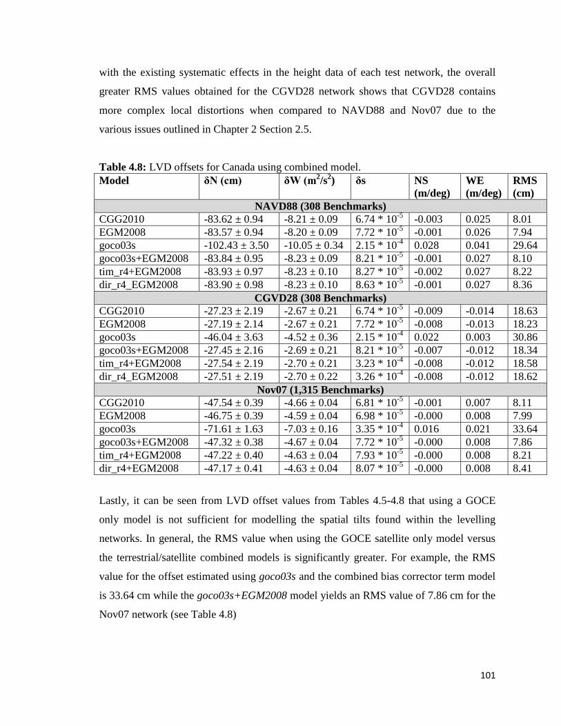
101
with the existing systematic effects in the height data of each test network, the overall
greater RMS values obtained for the CGVD28 network shows that CGVD28 contains
more complex local distortions when compared to NAVD88 and Nov07 due to the
various issues outlined in Chapter 2 Section 2.5.
Table 4.8: LVD offsets for Canada using combined model.
Model δN (cm) δW (m2/s
2) δs NS
(m/deg)
WE
(m/deg)
RMS
(cm)
NAVD88 (308 Benchmarks)
CGG2010 -83.62 ± 0.94 -8.21 ± 0.09 6.74 * 10-5
-0.003 0.025 8.01
EGM2008 -83.57 ± 0.94 -8.20 ± 0.09 7.72 * 10-5
-0.001 0.026 7.94
goco03s -102.43 ± 3.50 -10.05 ± 0.34 2.15 * 10-4
0.028 0.041 29.64
goco03s+EGM2008 -83.84 ± 0.95 -8.23 ± 0.09 8.21 * 10-5
-0.001 0.027 8.10
tim_r4+EGM2008 -83.93 ± 0.97 -8.23 ± 0.10 8.27 * 10-5
-0.002 0.027 8.22
dir_r4_EGM2008 -83.90 ± 0.98 -8.23 ± 0.10 8.63 * 10-5
-0.001 0.027 8.36
CGVD28 (308 Benchmarks)
CGG2010 -27.23 ± 2.19 -2.67 ± 0.21 6.74 * 10-5
-0.009 -0.014 18.63
EGM2008 -27.19 ± 2.14 -2.67 ± 0.21 7.72 * 10-5
-0.008 -0.013 18.23
goco03s -46.04 ± 3.63 -4.52 ± 0.36 2.15 * 10-4
0.022 0.003 30.86
goco03s+EGM2008 -27.45 ± 2.16 -2.69 ± 0.21 8.21 * 10-5
-0.007 -0.012 18.34
tim_r4+EGM2008 -27.54 ± 2.19 -2.70 ± 0.21 3.23 * 10-4
-0.008 -0.012 18.58
dir_r4_EGM2008 -27.51 ± 2.19 -2.70 ± 0.22 3.26 * 10-4
-0.008 -0.012 18.62
Nov07 (1,315 Benchmarks)
CGG2010 -47.54 ± 0.39 -4.66 ± 0.04 6.81 * 10-5
-0.001 0.007 8.11
EGM2008 -46.75 ± 0.39 -4.59 ± 0.04 6.98 * 10-5
-0.000 0.008 7.99
goco03s -71.61 ± 1.63 -7.03 ± 0.16 3.35 * 10-4
0.016 0.021 33.64
goco03s+EGM2008 -47.32 ± 0.38 -4.67 ± 0.04 7.72 * 10-5
-0.000 0.008 7.86
tim_r4+EGM2008 -47.22 ± 0.40 -4.63 ± 0.04 7.93 * 10-5
-0.000 0.008 8.21
dir_r4+EGM2008 -47.17 ± 0.41 -4.63 ± 0.04 8.07 * 10-5
-0.000 0.008 8.41
Lastly, it can be seen from LVD offset values from Tables 4.5-4.8 that using a GOCE
only model is not sufficient for modelling the spatial tilts found within the levelling
networks. In general, the RMS value when using the GOCE satellite only model versus
the terrestrial/satellite combined models is significantly greater. For example, the RMS
value for the offset estimated using goco03s and the combined bias corrector term model
is 33.64 cm while the goco03s+EGM2008 model yields an RMS value of 7.86 cm for the
Nov07 network (see Table 4.8)

102
Lastly, Tables 4.9-4.12 show the LVD offsets and the RMS error values computed using
the four bias corrector term models for the U.S.A. NAVD88 test network. Overall the
same trends are observed for the U.S.A. NAVD88 network as was discussed for the
NAVD88 and Nov07 test networks in Canada. Additionally, it can be observed from
Table 4.9 that the effect of the GOCE omission error on the LVD offset is approximately
2-3 cm, which can be ascribed to the density and configuration of the GNSS/levelling
benchmarks of the U.S.A. NAVD88 network.
Table 4.9: U.S.A. NAVD88 LVD offsets using null model.
Model δNj (cm) δW
j (m
2/s
2) RMS (cm)
CGG2010 -48.08 ± 0.22 -4.71 ± 0.02 29.94
USGG2012 -51.13 ± 0.22 -5.01 ± 0.02 29.93
EGM2008 -48.35 ± 0.22 -4.74 ± 0.02 30.05
goco03s -50.04 ± 0.39 -4.90 ± 0.04 52.60
goco03s+EGM2008 -48.38 ± 0.22 -4.74 ± 0.02 30.02
tim_r4 -50.77 ± 0.35 -4.98 ± 0.03 47.77
tim_r4+EGM2008 -48.06 ± 0.22 -4.71 ± 0.02 29.85
dir_r4 -51.00 ± 0.35 -5.00 ± 0.04 47.93
dir_r4+EGM2008 -48.29 ± 0.22 -4.73 ± 0.02 29.86
Table 4.10: U.S.A. NAVD88 LVD offsets using 1-parameter model.
Model δNj (cm) δW
j (m
2/s
2) δs RMS (cm)
CGG2010 -39.48 ± 0.25 -3.87 ± 0.03 -2.65 * 10-4
27.50
USGG2012 -42.66 ± 0.25 -4.18 ± 0.03 -2.61 * 10-4
27.57
EGM2008 -39.64 ± 0.25 -3.88 ± 0.03 -2.68 * 10-4
27.55
goco03s -40.06 ± 0.46 -3.93 ± 0.05 -3.07 * 10-4
50.77
goco03s+EGM2008 -39.74 ± 0.25 -3.89 ± 0.03 -2.66 * 10-4
27.56
tim_r4+EGM2008 -39.46 ± 0.25 -3.87 ± 0.02 -2.65 * 10-4
27.41
dir_r4+EGM2008 -39.71 ± 0.25 -3.89 ± 0.03 -2.64 * 10-4
27.43
Table 4.11: U.S.A. NAVD88 LVD offsets using 2-parameter model.
Model δNj (cm) δW
j (m
2/s
2) NS
(m/deg)
WE
(m/deg)
RMS
(cm)
CGG2010 -48.08 ± 0.05 -4.71 ± 0.02 -0.036 0.013 5.88
USGG2012 -51.13 ± 0.05 -5.01 ± 0.01 -0.036 0.013 6.10
EGM2008 -48.35 ± 0.05 -4.74 ± 0.02 -0.036 0.013 6.16
goco03s -50.04 ± 0.39 -4.90 ± 0.04 -0.031 0.021 41.46
goco03s+EGM2008 -48.38 ± 0.05 -4.74 ± 0.02 -0.035 0.013 6.50
tim_r4+EGM2008 -48.06 ± 0.05 -4.71 ± 0.01 -0.035 0.013 6.82
dir_r4+EGM2008 -48.29 ± 0.05 -4.73 ± 0.01 -0.035 0.013 6.97
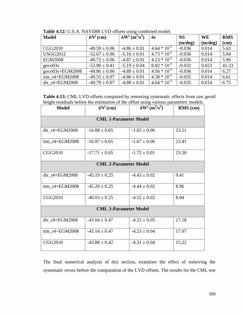
103
Table 4.12: U.S.A. NAVD88 LVD offsets using combined model.
Model δNj (cm) δW
j (m
2/s
2) δs NS
(m/deg)
WE
(m/deg)
RMS
(cm)
CGG2010 -49.59 ± 0.06 -4.86 ± 0.01 4.64 * 10-5
-0.036 0.014 5.63
USGG2012 -52.67 ± 0.06 -5.16 ± 0.01 4.73 * 10-5
-0.036 0.014 5.84
EGM2008 -49.72 ± 0.06 -4.87 ± 0.01 4.23 * 10-5
-0.036 0.014 5.96
goco03s -52.90 ± 0.41 -5.19 ± 0.04 8.82 * 10-5
-0.032 0.023 41.33
goco03s+EGM2008 -49.86 ± 0.06 -4.89 ± 0.01 4.56 * 10-5
-0.036 0.014 6.27
tim_r4+EGM2008 -49.55 ± 0.07 -4.86 ± 0.01 4.58 * 10-5
-0.035 0.014 6.61
dir_r4+EGM2008 -49.79 ± 0.07 -4.88 ± 0.01 4.64 * 10-5
-0.035 0.014 6.75
Table 4.13: CML LVD offsets computed by removing systematic effects from raw geoid
height residuals before the estimation of the offset using various parametric models.
Model δNj (cm) δW
j (m
2/s
2) RMS (cm)
CML 1-Parameter Model
dir_r4+EGM2008 -16.88 ± 0.65 -1.65 ± 0.06 23.51
tim_r4+EGM2008 -16.97 ± 0.65 -1.67 ± 0.06 23.41
CGG2010 -17.71 ± 0.65 -1.72 ± 0.01 23.50
CML 2-Parameter Model
dir_r4+EGM2008 -45.19 ± 0.25 -4.43 ± 0.02 9.41
tim_r4+EGM2008 -45.29 ± 0.25 -4.44 ± 0.02 8.96
CGG2010 -46.03 ± 0.25 -4.52 ± 0.02 8.94
CML 3-Parameter Model
dir_r4+EGM2008 -43.04 ± 0.47 -4.22 ± 0.05 17.18
tim_r4+EGM2008 -43.14 ± 0.47 -4.23 ± 0.04 17.07
CGG2010 -43.88 ± 0.42 -4.31 ± 0.04 15.22
The final numerical analysis of this section, examines the effect of removing the
systematic errors before the computation of the LVD offsets. The results for the CML test
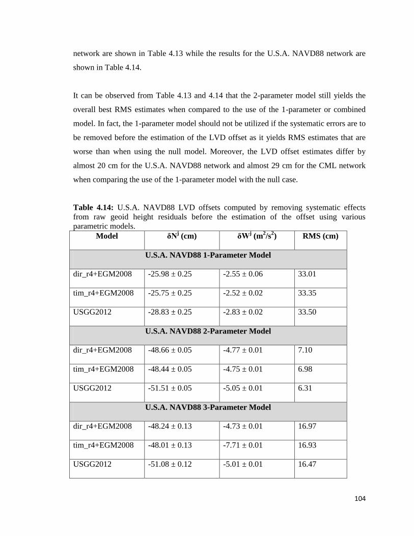
104
network are shown in Table 4.13 while the results for the U.S.A. NAVD88 network are
shown in Table 4.14.
It can be observed from Table 4.13 and 4.14 that the 2-parameter model still yields the
overall best RMS estimates when compared to the use of the 1-parameter or combined
model. In fact, the 1-parameter model should not be utilized if the systematic errors are to
be removed before the estimation of the LVD offset as it yields RMS estimates that are
worse than when using the null model. Moreover, the LVD offset estimates differ by
almost 20 cm for the U.S.A. NAVD88 network and almost 29 cm for the CML network
when comparing the use of the 1-parameter model with the null case.
Table 4.14: U.S.A. NAVD88 LVD offsets computed by removing systematic effects
from raw geoid height residuals before the estimation of the offset using various
parametric models.
Model δNj (cm) δW
j (m
2/s
2) RMS (cm)
U.S.A. NAVD88 1-Parameter Model
dir_r4+EGM2008 -25.98 ± 0.25 -2.55 ± 0.06 33.01
tim_r4+EGM2008 -25.75 ± 0.25 -2.52 ± 0.02 33.35
USGG2012 -28.83 ± 0.25 -2.83 ± 0.02 33.50
U.S.A. NAVD88 2-Parameter Model
dir_r4+EGM2008 -48.66 ± 0.05 -4.77 ± 0.01 7.10
tim_r4+EGM2008 -48.44 ± 0.05 -4.75 ± 0.01 6.98
USGG2012 -51.51 ± 0.05 -5.05 ± 0.01 6.31
U.S.A. NAVD88 3-Parameter Model
dir_r4+EGM2008 -48.24 ± 0.13 -4.73 ± 0.01 16.97
tim_r4+EGM2008 -48.01 ± 0.13 -7.71 ± 0.01 16.93
USGG2012 -51.08 ± 0.12 -5.01 ± 0.01 16.47
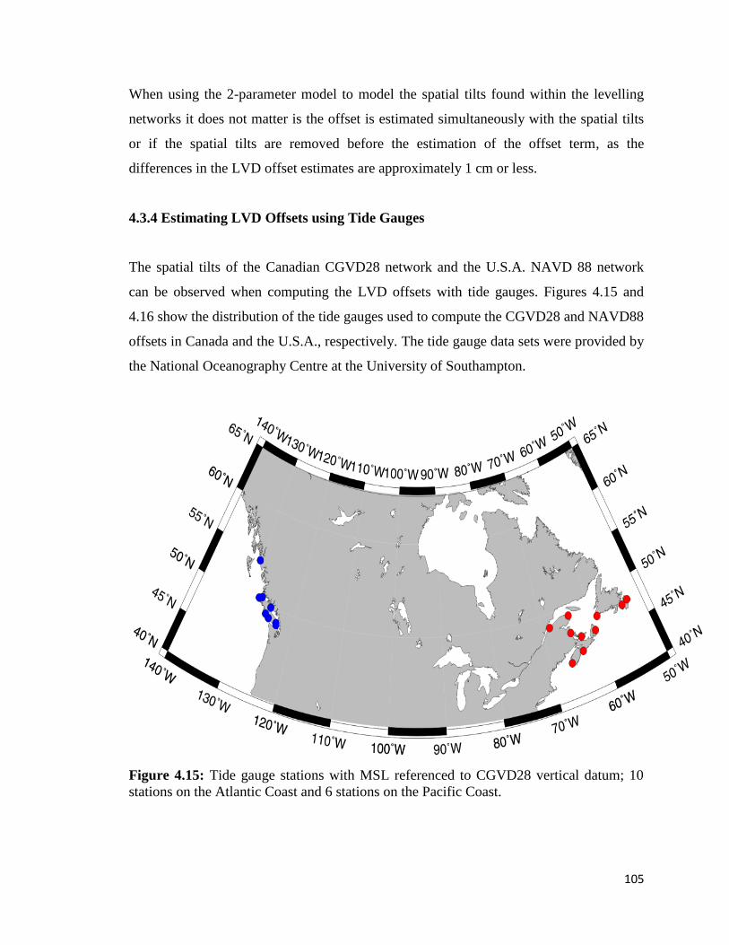
105
When using the 2-parameter model to model the spatial tilts found within the levelling
networks it does not matter is the offset is estimated simultaneously with the spatial tilts
or if the spatial tilts are removed before the estimation of the offset term, as the
differences in the LVD offset estimates are approximately 1 cm or less.
4.3.4 Estimating LVD Offsets using Tide Gauges
The spatial tilts of the Canadian CGVD28 network and the U.S.A. NAVD 88 network
can be observed when computing the LVD offsets with tide gauges. Figures 4.15 and
4.16 show the distribution of the tide gauges used to compute the CGVD28 and NAVD88
offsets in Canada and the U.S.A., respectively. The tide gauge data sets were provided by
the National Oceanography Centre at the University of Southampton.
Figure 4.15: Tide gauge stations with MSL referenced to CGVD28 vertical datum; 10
stations on the Atlantic Coast and 6 stations on the Pacific Coast.
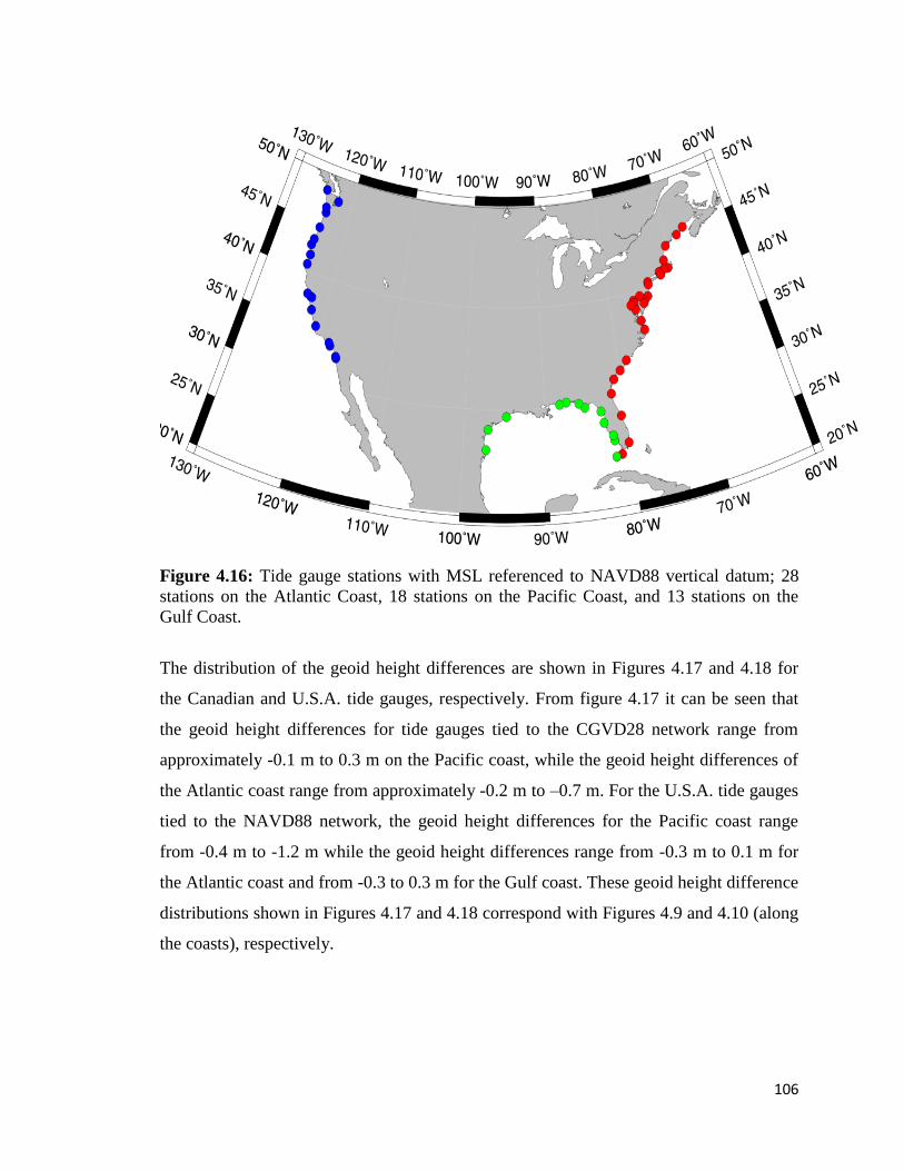
106
Figure 4.16: Tide gauge stations with MSL referenced to NAVD88 vertical datum; 28
stations on the Atlantic Coast, 18 stations on the Pacific Coast, and 13 stations on the
Gulf Coast.
The distribution of the geoid height differences are shown in Figures 4.17 and 4.18 for
the Canadian and U.S.A. tide gauges, respectively. From figure 4.17 it can be seen that
the geoid height differences for tide gauges tied to the CGVD28 network range from
approximately -0.1 m to 0.3 m on the Pacific coast, while the geoid height differences of
the Atlantic coast range from approximately -0.2 m to –0.7 m. For the U.S.A. tide gauges
tied to the NAVD88 network, the geoid height differences for the Pacific coast range
from -0.4 m to -1.2 m while the geoid height differences range from -0.3 m to 0.1 m for
the Atlantic coast and from -0.3 to 0.3 m for the Gulf coast. These geoid height difference
distributions shown in Figures 4.17 and 4.18 correspond with Figures 4.9 and 4.10 (along
the coasts), respectively.
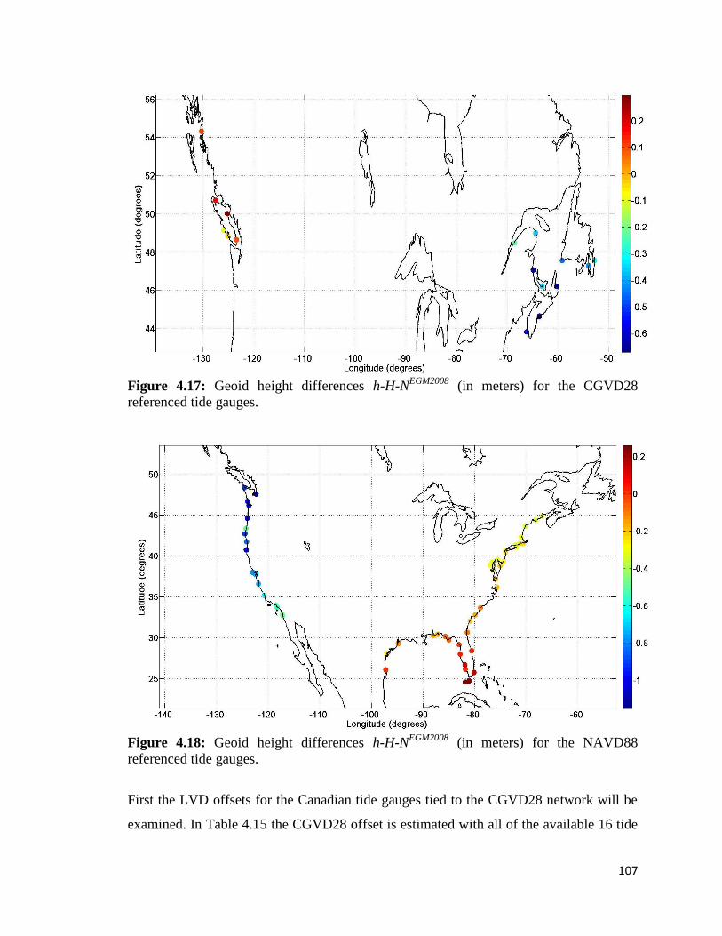
107
Figure 4.17: Geoid height differences h-H-N
EGM2008 (in meters) for the CGVD28
referenced tide gauges.
Figure 4.18: Geoid height differences h-H-N
EGM2008 (in meters) for the NAVD88
referenced tide gauges.
First the LVD offsets for the Canadian tide gauges tied to the CGVD28 network will be
examined. In Table 4.15 the CGVD28 offset is estimated with all of the available 16 tide
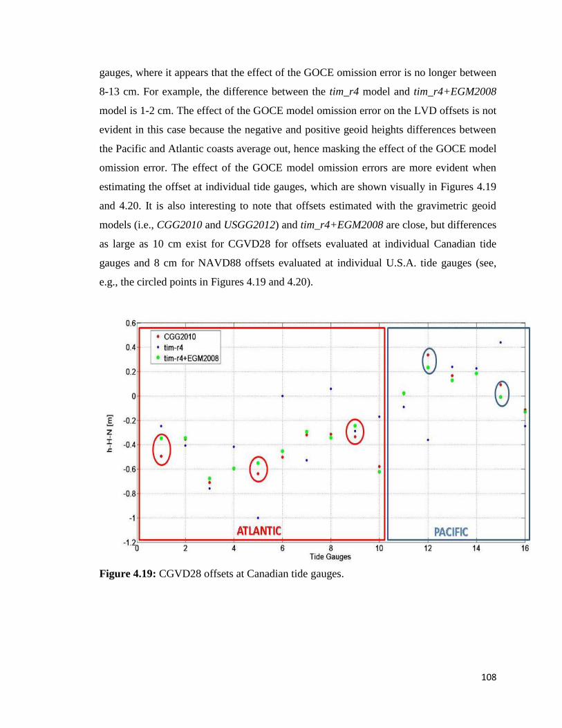
108
gauges, where it appears that the effect of the GOCE omission error is no longer between
8-13 cm. For example, the difference between the tim_r4 model and tim_r4+EGM2008
model is 1-2 cm. The effect of the GOCE model omission error on the LVD offsets is not
evident in this case because the negative and positive geoid heights differences between
the Pacific and Atlantic coasts average out, hence masking the effect of the GOCE model
omission error. The effect of the GOCE model omission errors are more evident when
estimating the offset at individual tide gauges, which are shown visually in Figures 4.19
and 4.20. It is also interesting to note that offsets estimated with the gravimetric geoid
models (i.e., CGG2010 and USGG2012) and tim_r4+EGM2008 are close, but differences
as large as 10 cm exist for CGVD28 for offsets evaluated at individual Canadian tide
gauges and 8 cm for NAVD88 offsets evaluated at individual U.S.A. tide gauges (see,
e.g., the circled points in Figures 4.19 and 4.20).
Figure 4.19: CGVD28 offsets at Canadian tide gauges.

109
Figure 4.20: NAVD88 offsets at U.S.A. tide gauges.
Table 4.15: CGVD28 offset with 16 Canadian tide gauges.
GGM δNj (cm) δW
j (m
2/s
2) W0
j (m
2/s
2)
tim_r4 -24.13 ± 10.69 -2.73 ± 1.05 62636858.37
tim_r4+EGM2008 -25.24 ± 7.41 -2.48 ± 0.73 62636858.48
EGM2008 -25.28 ± 7.75 -2.48 ± 0.76 62636858.48
CGG2010 -25.99 ± 8.31 -2.55 ± 0.82 62636858.55
Ince et al. -26.68 ± 8.42 -2.63 ± 0.83 62636858.62
Table 4.16: CGVD28 offset with 12 Canadian tide gauges.
GGM δNj (cm) δW
j (m
2/s
2) W0
j (m
2/s
2)
tim_r4 -27.81 ± 13.39 -2.73 ± 1.31 62636858.73
tim_r4+EGM2008 -24.70 ± 9.63 -2.43 ± 0.94 62636858.43
CGG2010 -24.35 ± 10.35 -2.39 ± 1.02 62636858.39
Ince et al. -25.51 ± 10.69 -2.50 ± 1.05 62636858.50
USGG2012 -26.08 ± 10.28 -2.56 ± 1.01 62636858.56
In Table 4.16, the offset is evaluated with 12 tide gauges in order to assess the CGVD28
offset estimated with the U.S.A. official gravimetric geoid model USGG2012 as 4 out of
the 16 Canadian tide gauges fall outside of the extent of the USGG2012 geoid grid.
Again, the same trends observed from the results in Table 4.15 are seen in Table 4.16.
The LVD offset estimated with USGG2012 differs by less than 1 cm when compared

110
with the gravimetric geoid model developed by Ince et al. (2012) while it differs by
approximately 2 cm when compared with CGG2010.
Tables 4.17 and 4.18 show LVD offsets estimated using 2 high quality tide gauges from
the Atlantic and 5 high quality tide gauges from the Pacific that are in common with the
tide gauge data set utilized for W0 evaluation in Chapter 5. In this case, “high quality”
refers to a tide gauge that has long term daily water level records without significant data
gaps for the accurate evaluation of MSL. Specifically, the tide gauge stations utilized for
the computation of LVD offsets in the Atlantic are stations 365 and 2330 while for the
Pacific the tide gauges correspond to stations 8408, 9354, 8074, 8615, and 8545 (see
Chapter 5, Table 5.1).
Table 4.17: CGVD28 offset with 2 Canadian tide gauges (Atlantic).
GGM δNj (cm) δW
j (m
2/s
2) W0
j (m
2/s
2)
goco03s -7.11 ± 9.38 -0.70 ± 0.92 62636856.70
goco3s+EGM2008 -49.55 ± 4.01 -4.86 ± 0.40 62636860.86
tim_r4 -5.01 ± 9.87 -0.49 ± 0.97 62636856.49
tim_r4+EGM2008 -47.45 ± 4.50 -4.66 ± 0.44 62636860.66
EGM2008 -49.12 ± 5.25 -4.82 ± 0.52 62636860.82
CGG2010 -44.66 ± 5.37 -4.38 ± 0.53 62636860.38
Ince et al. -48.53 ± 3.97 -4.76 ± 0.39 62636860.76
Table 4.18: CGVD28 offset with 5 Canadian tide gauges (Pacific).
GGM δNj (cm) δW
j (m
2/s
2) W0
j (m
2/s
2)
goco03s -2.82 ± 12.44 -0.28 ± 1.22 62636856.28
goco3s+EGM2008 6.26 ± 5.38 -0.61 ± 0.53 62636855.39
tim_r4 -1.76 ± 12.40 -0.17 ± 1.21 62636856.17
tim_r4+EGM2008 7.34 ± 5.32 0.72 ± 0.52 62636855.28
EGM2008 9.02 ± 5.85 0.88 ± 0.57 62636855.12
CGG2010 10.46 ± 6.22 1.02 ± 0.61 62636854.97
Ince et al. 10.62 ± 5.93 1.04 ± 0.58 62636854.96
From the results presented in Tables 4.17 and 4.18 it is evident that utilizing only
goco03s or the tim_r4 model only is not sufficient for estimating LVD offset; the offsets
computed with goco03s or tim_r4 yields a statistically insignificant LVD offsets as the
estimated LVD offsets are smaller than three times their formal errors. For example, the
CGVD28 offset for the Atlantic is -5.01 ± 9.87 cm and for the Pacific it is -1.76 ± 12.40
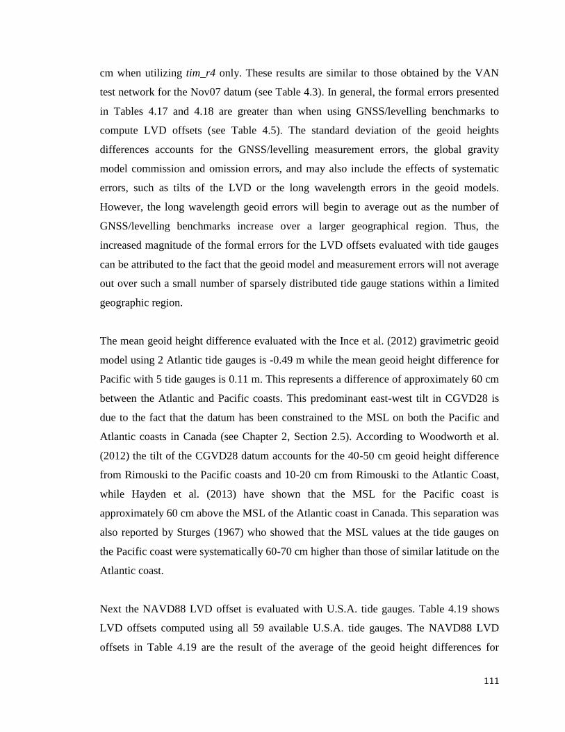
111
cm when utilizing tim_r4 only. These results are similar to those obtained by the VAN
test network for the Nov07 datum (see Table 4.3). In general, the formal errors presented
in Tables 4.17 and 4.18 are greater than when using GNSS/levelling benchmarks to
compute LVD offsets (see Table 4.5). The standard deviation of the geoid heights
differences accounts for the GNSS/levelling measurement errors, the global gravity
model commission and omission errors, and may also include the effects of systematic
errors, such as tilts of the LVD or the long wavelength errors in the geoid models.
However, the long wavelength geoid errors will begin to average out as the number of
GNSS/levelling benchmarks increase over a larger geographical region. Thus, the
increased magnitude of the formal errors for the LVD offsets evaluated with tide gauges
can be attributed to the fact that the geoid model and measurement errors will not average
out over such a small number of sparsely distributed tide gauge stations within a limited
geographic region.
The mean geoid height difference evaluated with the Ince et al. (2012) gravimetric geoid
model using 2 Atlantic tide gauges is -0.49 m while the mean geoid height difference for
Pacific with 5 tide gauges is 0.11 m. This represents a difference of approximately 60 cm
between the Atlantic and Pacific coasts. This predominant east-west tilt in CGVD28 is
due to the fact that the datum has been constrained to the MSL on both the Pacific and
Atlantic coasts in Canada (see Chapter 2, Section 2.5). According to Woodworth et al.
(2012) the tilt of the CGVD28 datum accounts for the 40-50 cm geoid height difference
from Rimouski to the Pacific coasts and 10-20 cm from Rimouski to the Atlantic Coast,
while Hayden et al. (2013) have shown that the MSL for the Pacific coast is
approximately 60 cm above the MSL of the Atlantic coast in Canada. This separation was
also reported by Sturges (1967) who showed that the MSL values at the tide gauges on
the Pacific coast were systematically 60-70 cm higher than those of similar latitude on the
Atlantic coast.
Next the NAVD88 LVD offset is evaluated with U.S.A. tide gauges. Table 4.19 shows
LVD offsets computed using all 59 available U.S.A. tide gauges. The NAVD88 LVD
offsets in Table 4.19 are the result of the average of the geoid height differences for
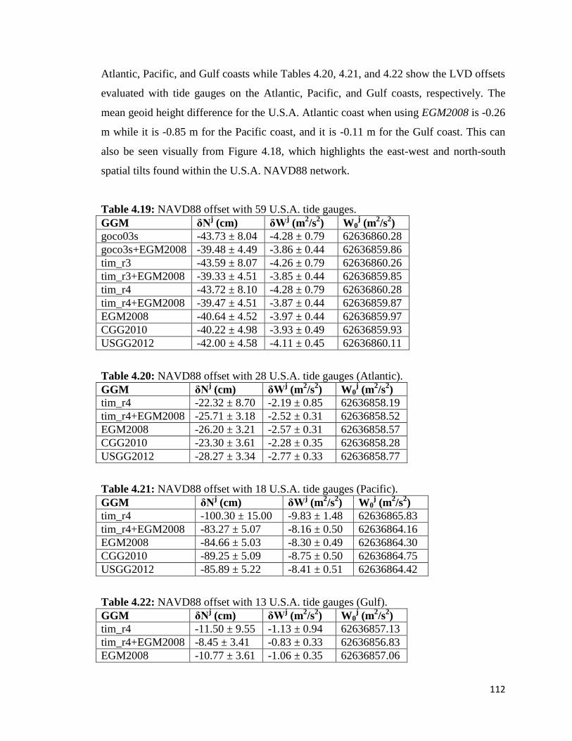
112
Atlantic, Pacific, and Gulf coasts while Tables 4.20, 4.21, and 4.22 show the LVD offsets
evaluated with tide gauges on the Atlantic, Pacific, and Gulf coasts, respectively. The
mean geoid height difference for the U.S.A. Atlantic coast when using EGM2008 is -0.26
m while it is -0.85 m for the Pacific coast, and it is -0.11 m for the Gulf coast. This can
also be seen visually from Figure 4.18, which highlights the east-west and north-south
spatial tilts found within the U.S.A. NAVD88 network.
Table 4.19: NAVD88 offset with 59 U.S.A. tide gauges.
GGM δNj (cm) δW
j (m
2/s
2) W0
j (m
2/s
2)
goco03s -43.73 ± 8.04 -4.28 ± 0.79 62636860.28
goco3s+EGM2008 -39.48 ± 4.49 -3.86 ± 0.44 62636859.86
tim_r3 -43.59 ± 8.07 -4.26 ± 0.79 62636860.26
tim_r3+EGM2008 -39.33 ± 4.51 -3.85 ± 0.44 62636859.85
tim_r4 -43.72 ± 8.10 -4.28 ± 0.79 62636860.28
tim_r4+EGM2008 -39.47 ± 4.51 -3.87 ± 0.44 62636859.87
EGM2008 -40.64 ± 4.52 -3.97 ± 0.44 62636859.97
CGG2010 -40.22 ± 4.98 -3.93 ± 0.49 62636859.93
USGG2012 -42.00 ± 4.58 -4.11 ± 0.45 62636860.11
Table 4.20: NAVD88 offset with 28 U.S.A. tide gauges (Atlantic).
GGM δNj (cm) δW
j (m
2/s
2) W0
j (m
2/s
2)
tim_r4 -22.32 ± 8.70 -2.19 ± 0.85 62636858.19
tim_r4+EGM2008 -25.71 ± 3.18 -2.52 ± 0.31 62636858.52
EGM2008 -26.20 ± 3.21 -2.57 ± 0.31 62636858.57
CGG2010 -23.30 ± 3.61 -2.28 ± 0.35 62636858.28
USGG2012 -28.27 ± 3.34 -2.77 ± 0.33 62636858.77
Table 4.21: NAVD88 offset with 18 U.S.A. tide gauges (Pacific).
GGM δNj (cm) δW
j (m
2/s
2) W0
j (m
2/s
2)
tim_r4 -100.30 ± 15.00 -9.83 ± 1.48 62636865.83
tim_r4+EGM2008 -83.27 ± 5.07 -8.16 ± 0.50 62636864.16
EGM2008 -84.66 ± 5.03 -8.30 ± 0.49 62636864.30
CGG2010 -89.25 ± 5.09 -8.75 ± 0.50 62636864.75
USGG2012 -85.89 ± 5.22 -8.41 ± 0.51 62636864.42
Table 4.22: NAVD88 offset with 13 U.S.A. tide gauges (Gulf).
GGM δNj (cm) δW
j (m
2/s
2) W0
j (m
2/s
2)
tim_r4 -11.50 ± 9.55 -1.13 ± 0.94 62636857.13
tim_r4+EGM2008 -8.45 ± 3.41 -0.83 ± 0.33 62636856.83
EGM2008 -10.77 ± 3.61 -1.06 ± 0.35 62636857.06

113
GGM δNj (cm) δW
j (m
2/s
2) W0
j (m
2/s
2)
CGG2010 -8.77 ± 4.31 -0.86 ± 0.42 62636856.86
USGG2012 -10.78 ± 3.80 -1.06 ± 0.37 62636857.06
4.4 Summary
The objective of this chapter was to study the performance of the most recent GOCE-
based GGMs for the purpose of computing the potential and height datum offset of the
CGVD28, NAVD88, and Nov07 levelling-based vertical datums. In order to accomplish
this, the potential and geoid height differences were evaluated with a GOCE only satellite
model (i.e., tim_r4), GOCE-GRACE satellite models (i.e., goco03s and dir_r4), a
GRACE only model (i.e., itg-grace2010s), the high resolution gravity field model
EGM2008, and the regional gravimetric geoid models CGG2010, USGG2012, and Ince et
al. (2012).
With the goal to unify vertical datums with 1 cm accuracy it can be concluded that the
effect of the truncation degree of the GOCE model is an important factor. In Canada, the
effect of the GOCE omission error ranges between 8 and 13 cm for LVD offset
computations. This can be attributed to the irregular and spare distribution of the
GNSS/levelling benchmarks found in the Canadian test networks, in particular, for
regions such as western Canada where the topography is quite rugged. The effect of the
GOCE omission error on LVD offset estimation indicates that the contributions of the
higher frequencies of the gravity field is very important when evaluating the potential and
the height offsets of the Nov07, NAVD88, and CGVD28 datums using Canadian
GNSS/levelling benchmark information and GOCE GGMs. In contrast, the effect of the
GOCE omission error on LVD offsets is less significant in the U.S.A. when using
GNSS/levelling information; the effect is only 2-3 cm and can be explained by the fact
that the U.S.A. test network contains a dense and homogenous distribution of
GNSS/levelling benchmarks that covers an appreciably large geographical area.
However, as the objective is to unify vertical datums with 1 cm accuracy, the effect of the
GOCE omission error on the LVD offsets for the U.S.A. NAVD88 network should
therefore also be taken into account.
114
Additionally, the effect of the ellipsoidal, levelling, and geoid height errors contribute up
to 4 cm to LVD offsets computed over the Canadian mainland, and can have a dm-level
impact for island regions. Therefore, in addition to including the accuracy information of
the GNSS/levelling data and GGM coefficients, the residual geoid heights should ideally
be evaluated with Stokes integration using local gravity data. The high frequency
contribution of the topography should also be taken into account using a remove-
compute-restore scheme where a GOCE-GRACE combination model can contribute to
the long to medium wavelength components of the gravity field signal. The inclusion of
these factors is necessary when using the GNSS/levelling data over the Canadian
mainland to compute the LVD offsets, and are especially important for regions with very
few benchmarks, limited geographical coverage, and/or rugged terrain, such as
independent levelling networks on islands, where the geoid model errors and the
measurement errors of the GNSS/levelling heights are not likely to average out. Hence,
the inclusion of these factors should be considered for future investigations.
Using tide gauges with MSL referenced to CGVD28 in Canada and NAVD88 in U.S.A.
to compute LVD offsets emphasizes the spatial tilts found within each network. For both
networks the mean geoid height differences differ by approximately 60 cm between the
Atlantic and Pacific coasts. For the CGVD28 network that is constrained by multiple tide
gauges on the Atlantic and Pacific coasts this difference coincides with the difference in
MSL between the two coasts whereas the U.S.A. NAVD88 network is only constrained
to the height of the primary tidal benchmark at Rimouski, Quebec (Zilkoski et al. 1992),
meaning that the geoid height differences and the potentials evaluated for either coast
does not necessarily coincide with the potential of the MSL (which will be examined in
Chapter 5).
Due to the existence of the spatial tilts in levelling networks, the removal of systematic
effects from the height data is an important step for the computation of LVD offsets. For
the Canadian mainland GNSS/levelling networks both a small north-south spatial tilt and
a relatively larger west-east spatial tilt exist in the Nov07 and NAVD88 datums, which
115
can be modelled with a 2-parameter bias corrector term model as it yields the smallest
RMS value for the adjusted geoid height residuals. Likewise, in the U.S.A. both a north-
south and west-east spatial tilt is present within the NAVD88 network, which can also be
modelled using the 2-parameter bias corrector term model. When using the 2-parameter
model, the spatial tilts may be estimated either before or simultaneously along with the
offset term as the difference between these methods on the LVD offset estimate reaches a
maximum of 1 cm depending on the geoid model utilized.
For the CGVD28 network, it is recommended that further investigations into the local
distortions and systematic effects are likely necessary, as the LVD offset values differed
quite significantly between the use of the different bias corrector term models. Moreover,
the RMS value remained close to 20 cm when computing LVD offsets using all three
different bias corrector term models, which is approximately 10 cm greater than the RMS
values for the Canadian NAVD88 and Nov07 networks for the 2-parameter and
combined model cases. Including a larger number of GNSS/levelling benchmarks into the
analysis could also be a factor in modeling the systematic effects in the CGVD28
network, if indeed the systematic effects follow a more complex pattern than simple
spatial tilts.
116
CHAPTER 5
EVALUATION OF W0 USING CANADIAN TIDE GAUGES AND GOCE
GLOBAL GEOPOTENTIAL MODELS
5.1 Introduction
One of the key factors in the implementation of the geoid-based vertical datum in Canada
is to have a common datum with the U.S.A., and by extension a common geoid model for
North America. Therefore, one of the primary concerns in choosing a common geoid
model is to jointly agree upon which W0 value should be chosen as the zero height
surface. In order to satisfy the definition that the geoid is the level surface of constant
gravity potential that best represents the MSL at rest, the W0 value can be evaluated by
averaging the potentials of points on the mean water surface, which can be computed
from the mean sea surface topography that is referenced to an equipotential surface with a
known potential.
There are three basic options for obtaining the sea surface topography:
1) the combination of tide gauge records and a geoid model,
2) the combination of satellite altimetry sea surface heights and a geoid model,
3) and oceanic sea surface topography models.
Sea surface topography models are generally estimated from satellite altimetry and
geodetic measurements, but may also include measurements such as seawater
temperature, salinity data, tide gauge observations, and ocean surface drifter velocities
(e.g., Rapp and Wang 1994; Ekman and Mäkinen 1996; Rio et al. 2004; Bingham and
Haines 2006; Thompson and Demirov 2006; Foreman et al. 2008; Anderson and
Knudsen 2009; Maximenko et al. 2009; Thompson et al. 2009, among others). For the
most part, W0 has been computed globally using satellite altimetry observations (e.g.,
Burša et al. 1998; Sánchez 2009; Dayoub et al. 2012; Yonghai and Jiancheng 2012), and
to a lesser extent, the geopotential at tide gauges has also been used to determine regional

117
W0 (e.g. Grafarend and Ardalan 1997; Ardalan et al. 2002; Bolkas et al. 2012; Hayden et
al. 2012b; Hayden et al. 2013).
In order to avoid inconsistencies included in terrestrial gravity data due to the use of
different height datums when estimating W0, the use of a satellite only global geopotential
model (GGM) is preferred. The focus of this chapter is the determination of the W0 for
the new Canadian vertical datum utilizing recently released satellite-only GOCE GGMs
in combination with tide gauge records. As previously discussed in Chapter 3 and
Chapter 4, the effect of the omission errors of the GOCE satellite only models may be
significant at the tide gauge locations along the Canadian coasts and may bias the mean
potential of the local mean sea level. In order to quantify the approximate omission errors
resulting from GOCE-only global geopotential models, W0 is also computed with the use
of high resolution geoid models (e.g., CGG2010 (Huang and Véronneau 2013) and
EGM2008 (Pavlis et al. 2012)). Specifically, contributions of Canadian tide gauges for
the determination of W0 are examined by averaging the potential of points on the mean
water surface evaluated from the geometrical mean sea surface topography using tide
gauge records that have been averaged over 19 years (in order to eliminate the variations
due to the tides) with the effects of sea level rise and vertical land motion accounted for.
Furthermore, regional SST models are utilized as an independent approach for validating
W0 results obtained from tide gauges and gravity field models. Additionally, a wide range
of global SST models are also used to validate the W0 results obtained from the tide
gauge records.
5.2 Methodology
The basic procedure for computing W0 value through tide gauge averaging can be
outlined as follows:
1) Selection of tide gauges which have been surveyed with GNSS;
2) Selection of a geoid model;
3) Computation of the gravity potential W of the local mean sea level height at each
respective tide gauge; and
118
4) Computation of W0 as the mean W value from all the tide gauges.
5.2.1 Distribution of Tide Gauge Stations and Water Level Data
The determination of MSL requires the removal of all periodic constituents existing in
the tide gauge record, where the longest constituent is the lunar nodal tidal constituent of
18.6 years. Therefore, a near uniform distribution of tide gauge stations with up to date
long-term time series, preferably up to one lunar nodal cycle (i.e., approximately19 years)
or multiples of this cycle, is ideal in order to obtain a W value that best represents the
MSL around the Canadian coastline. Furthermore, the 19-year data span will also average
out effects of sea levels due to weather such as wind stress, changes in atmospheric
pressure, and storm events (Pugh 1987).
Tide gauges along the Canadian Pacific, Atlantic, and Arctic coasts were selected for the
determination of the mean W0 value based on the following criteria:
1) The tide gauge has a corresponding benchmark which has been surveyed with
GNSS;
2) The tide gauge benchmark should be in good condition according to the Canadian
Hydrographic Service (CHS); and
3) The tide gauge has water level data for 19 years from 1992 to 2011 without
significant data gaps (i.e., no more than 2-3 years of missing data).
Only a small portion of tide gauges available in Canada meet the above criteria for the
determination of W0. Specifically, there are 12 tide gauges in the Pacific, 10 tide gauges
in the Atlantic, and 1 tide gauge in the Arctic that contain 19 years of water level data. In
order to extend the analysis the Arctic, tide gauges with at least 12 months of data after
1990 were also included, and the local MSL was computed from monthly water level
data obtained from the CHS, thus there are 38 tide gauges in total. The final list of
stations used is given in Table 5.1 and the geographic distribution of the tide gauges is
shown in Figure 5.1.
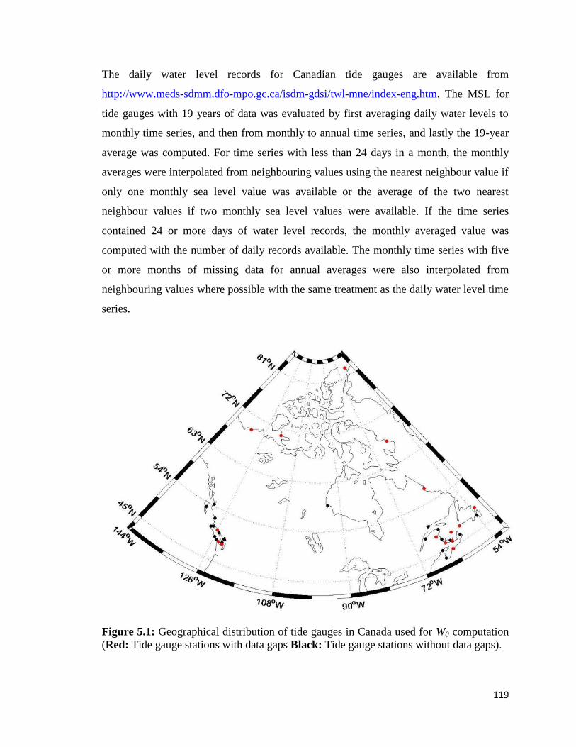
119
The daily water level records for Canadian tide gauges are available from
http://www.meds-sdmm.dfo-mpo.gc.ca/isdm-gdsi/twl-mne/index-eng.htm. The MSL for
tide gauges with 19 years of data was evaluated by first averaging daily water levels to
monthly time series, and then from monthly to annual time series, and lastly the 19-year
average was computed. For time series with less than 24 days in a month, the monthly
averages were interpolated from neighbouring values using the nearest neighbour value if
only one monthly sea level value was available or the average of the two nearest
neighbour values if two monthly sea level values were available. If the time series
contained 24 or more days of water level records, the monthly averaged value was
computed with the number of daily records available. The monthly time series with five
or more months of missing data for annual averages were also interpolated from
neighbouring values where possible with the same treatment as the daily water level time
series.
Figure 5.1: Geographical distribution of tide gauges in Canada used for W0 computation
(Red: Tide gauge stations with data gaps Black: Tide gauge stations without data gaps).
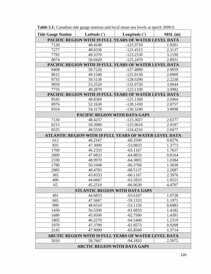
120
Table 5.1: Canadian tide gauge stations and local mean sea levels at epoch 2008.0.
Tide Gauge Station Latitude (˚) Longitude (˚) MSL (m)
PACIFIC REGION WITH 19 FULL YEARS OF WATER LEVEL DATA
7120 48.4240 -123.3710 1.9201
7277 48.6536 -123.4515 2.3137
7795 49.3370 -123.2530 3.1190
8074 50.0420 -125.2470 2.8931
PACIFIC REGION WITH 19 FULL YEARS OF WATER LEVEL DATA
8408 50.7220 -127.4890 2.9059
8615 49.1540 -125.9130 2.0909
8735 50.5130 -128.0290 2.2238
9850 53.2520 -132.0720 3.9944
7735 49.2870 -123.1100 3.0982
PACIFIC REGION WITH 19 FULL YEARS OF WATER LEVEL DATA
8545 48.8360 -125.1360 2.0464
8976 52.1630 -128.1430 2.8757
9354 54.3170 -130.3240 3.9098
PACIFIC REGION WITH DATA GAPS
7130 48.4237 -123.3027 2.0277
8215 50.3980 -125.9610 2.9197
8525 48.5550 -124.4210 2.0477
ATLANTIC REGION WITH 19 FULL YEARS OF WATER LEVEL DATA
612 46.2167 -60.2500 0.8276
835 47.3000 -53.9833 1.3773
1700 46.2333 -63.1167 1.7657
2000 47.0833 -64.8833 0.8164
2330 48.9970 -64.3805 1.0384
2780 50.1948 -66.3768 1.5838
2985 48.4783 -68.5137 2.2687
365 43.8333 -66.1167 2.5976
490 44.6667 -63.5833 1.0551
65 45.2510 -66.0630 4.4707
ATLANTIC REGION WITH DATA GAPS
491 44.6833 -63.6167 1.0728
665 47.5667 -59.1333 1.1971
990 48.6510 -53.1150 0.6083
1430 56.5500 -61.6833 1.4182
1680 45.9500 -62.7500 1.4391
1805 46.2270 -64.5460 1.2319
1970 47.3789 -61.8573 0.9209
2145 47.9000 -65.8500 1.3714
ARCTIC REGION WITH 19 FULL YEARS OF WATER LEVEL DATA
5010 58.7667 -94.1833 2.5972
ARCTIC REGION WITH DATA GAPS
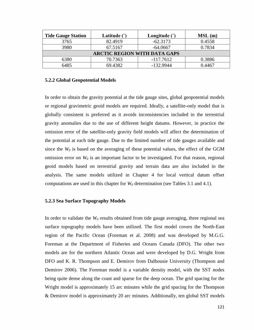
121
Tide Gauge Station Latitude (˚) Longitude (˚) MSL (m)
3765 82.4919 -62.3173 0.4558
3980 67.5167 -64.0667 0.7834
ARCTIC REGION WITH DATA GAPS
6380 70.7363 -117.7612 0.3886
6485 69.4382 -132.9944 0.4467
5.2.2 Global Geopotential Models
In order to obtain the gravity potential at the tide gauge sites, global geopotential models
or regional gravimetric geoid models are required. Ideally, a satellite-only model that is
globally consistent is preferred as it avoids inconsistencies included in the terrestrial
gravity anomalies due to the use of different height datums. However, in practice the
omission error of the satellite-only gravity field models will affect the determination of
the potential at each tide gauge. Due to the limited number of tide gauges available and
since the W0 is based on the averaging of these potential values, the effect of the GGM
omission error on W0 is an important factor to be investigated. For that reason, regional
geoid models based on terrestrial gravity and terrain data are also included in the
analysis. The same models utilized in Chapter 4 for local vertical datum offset
computations are used in this chapter for W0 determination (see Tables 3.1 and 4.1).
5.2.3 Sea Surface Topography Models
In order to validate the W0 results obtained from tide gauge averaging, three regional sea
surface topography models have been utilized. The first model covers the North-East
region of the Pacific Ocean (Foreman et al. 2008) and was developed by M.G.G.
Foreman at the Department of Fisheries and Oceans Canada (DFO). The other two
models are for the northern Atlantic Ocean and were developed by D.G. Wright from
DFO and K. R. Thompson and E. Demirov from Dalhousie University (Thompson and
Demirov 2006). The Foreman model is a variable density model, with the SST nodes
being quite dense along the coast and sparse for the deep ocean. The grid spacing for the
Wright model is approximately 15 arc minutes while the grid spacing for the Thompson
& Demirov model is approximately 20 arc minutes. Additionally, ten global SST models
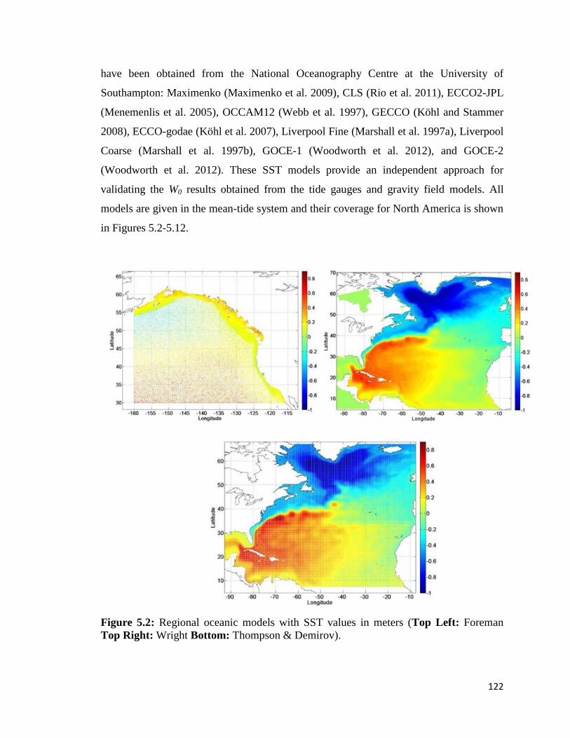
122
have been obtained from the National Oceanography Centre at the University of
Southampton: Maximenko (Maximenko et al. 2009), CLS (Rio et al. 2011), ECCO2-JPL
(Menemenlis et al. 2005), OCCAM12 (Webb et al. 1997), GECCO (Köhl and Stammer
2008), ECCO-godae (Köhl et al. 2007), Liverpool Fine (Marshall et al. 1997a), Liverpool
Coarse (Marshall et al. 1997b), GOCE-1 (Woodworth et al. 2012), and GOCE-2
(Woodworth et al. 2012). These SST models provide an independent approach for
validating the W0 results obtained from the tide gauges and gravity field models. All
models are given in the mean-tide system and their coverage for North America is shown
in Figures 5.2-5.12.
Figure 5.2: Regional oceanic models with SST values in meters (Top Left: Foreman
Top Right: Wright Bottom: Thompson & Demirov).
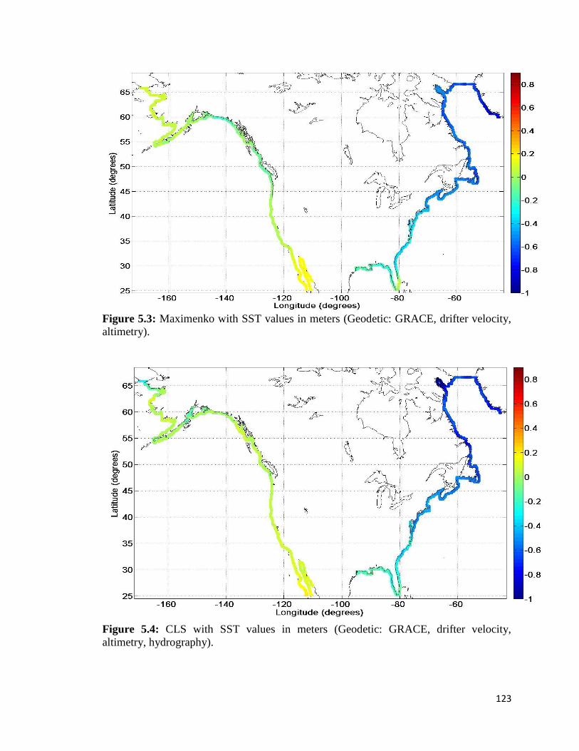
123
Figure 5.3: Maximenko with SST values in meters (Geodetic: GRACE, drifter velocity,
altimetry).
Figure 5.4: CLS with SST values in meters (Geodetic: GRACE, drifter velocity,
altimetry, hydrography).
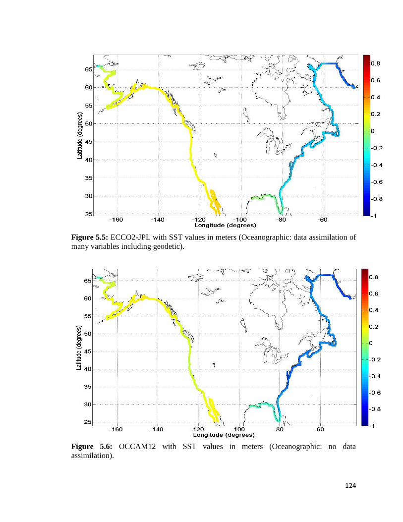
124
Figure 5.5: ECCO2-JPL with SST values in meters (Oceanographic: data assimilation of
many variables including geodetic).
Figure 5.6: OCCAM12 with SST values in meters (Oceanographic: no data
assimilation).
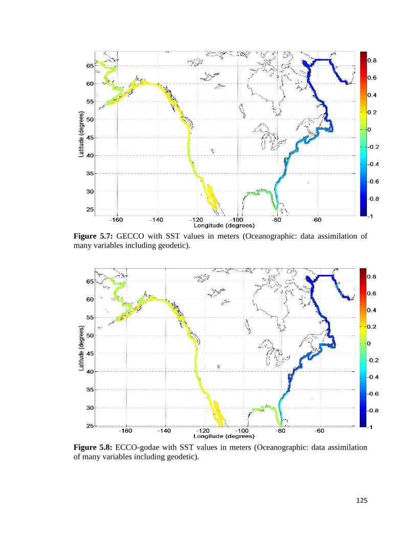
125
Figure 5.7: GECCO with SST values in meters (Oceanographic: data assimilation of
many variables including geodetic).
Figure 5.8: ECCO-godae with SST values in meters (Oceanographic: data assimilation
of many variables including geodetic).
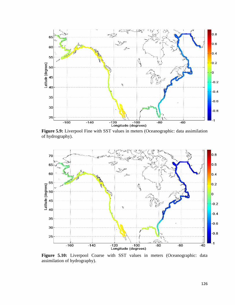
126
Figure 5.9: Liverpool Fine with SST values in meters (Oceanographic: data assimilation
of hydrography).
Figure 5.10: Liverpool Coarse with SST values in meters (Oceanographic: data
assimilation of hydrography).
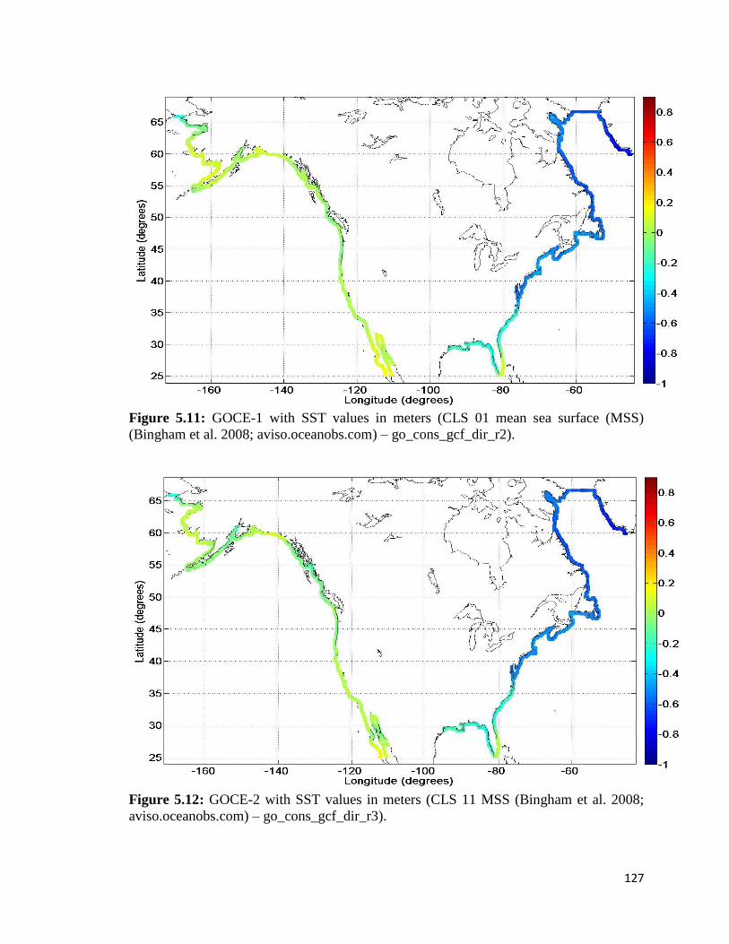
127
Figure 5.11: GOCE-1 with SST values in meters (CLS 01 mean sea surface (MSS)
(Bingham et al. 2008; aviso.oceanobs.com) – go_cons_gcf_dir_r2).
Figure 5.12: GOCE-2 with SST values in meters (CLS 11 MSS (Bingham et al. 2008;
aviso.oceanobs.com) – go_cons_gcf_dir_r3).
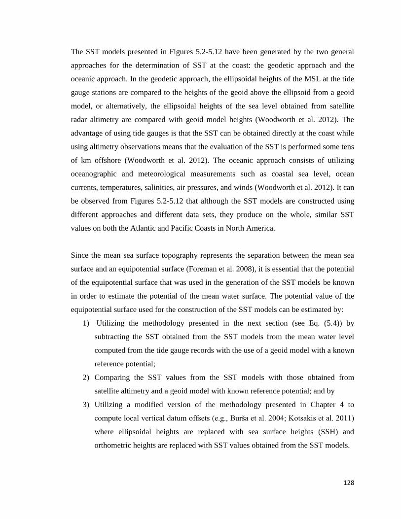
128
The SST models presented in Figures 5.2-5.12 have been generated by the two general
approaches for the determination of SST at the coast: the geodetic approach and the
oceanic approach. In the geodetic approach, the ellipsoidal heights of the MSL at the tide
gauge stations are compared to the heights of the geoid above the ellipsoid from a geoid
model, or alternatively, the ellipsoidal heights of the sea level obtained from satellite
radar altimetry are compared with geoid model heights (Woodworth et al. 2012). The
advantage of using tide gauges is that the SST can be obtained directly at the coast while
using altimetry observations means that the evaluation of the SST is performed some tens
of km offshore (Woodworth et al. 2012). The oceanic approach consists of utilizing
oceanographic and meteorological measurements such as coastal sea level, ocean
currents, temperatures, salinities, air pressures, and winds (Woodworth et al. 2012). It can
be observed from Figures 5.2-5.12 that although the SST models are constructed using
different approaches and different data sets, they produce on the whole, similar SST
values on both the Atlantic and Pacific Coasts in North America.
Since the mean sea surface topography represents the separation between the mean sea
surface and an equipotential surface (Foreman et al. 2008), it is essential that the potential
of the equipotential surface that was used in the generation of the SST models be known
in order to estimate the potential of the mean water surface. The potential value of the
equipotential surface used for the construction of the SST models can be estimated by:
1) Utilizing the methodology presented in the next section (see Eq. (5.4)) by
subtracting the SST obtained from the SST models from the mean water level
computed from the tide gauge records with the use of a geoid model with a known
reference potential;
2) Comparing the SST values from the SST models with those obtained from
satellite altimetry and a geoid model with known reference potential; and by
3) Utilizing a modified version of the methodology presented in Chapter 4 to
compute local vertical datum offsets (e.g., Burša et al. 2004; Kotsakis et al. 2011)
where ellipsoidal heights are replaced with sea surface heights (SSH) and
orthometric heights are replaced with SST values obtained from the SST models.
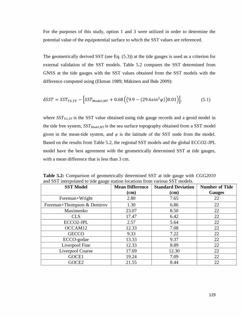
129
For the purposes of this study, option 1 and 3 were utilized in order to determine the
potential value of the equipotential surface to which the SST values are referenced.
The geometrically derived SST (see Eq. (5.3)) at the tide gauges is used as a criterion for
external validation of the SST models. Table 5.2 compares the SST determined from
GNSS at the tide gauges with the SST values obtained from the SST models with the
difference computed using (Ekman 1989; Mäkinen and Ihde 2009):
[ (( ) )] (5.1)
where SSTTG,TF is the SST value obtained using tide gauge records and a geoid model in
the tide free system, SSTModel,MT is the sea surface topography obtained from a SST model
given in the mean-tide system, and φ is the latitude of the SST node from the model.
Based on the results from Table 5.2, the regional SST models and the global ECCO2-JPL
model have the best agreement with the geometrically determined SST at tide gauges,
with a mean difference that is less than 3 cm.
Table 5.2: Comparison of geometrically determined SST at tide gauge with CGG2010
and SST interpolated to tide gauge station locations from various SST models.
SST Model Mean Difference
(cm)
Standard Deviation
(cm)
Number of Tide
Gauges
Foreman+Wright 2.80 7.65 22
Foreman+Thompson & Demirov 1.30 6.86 22
Maximenko 23.07 8.50 22
CLS 17.47 6.42 22
ECCO2-JPL 2.57 5.64 22
OCCAM12 12.33 7.08 22
GECCO 9.33 7.22 22
ECCO-godae 13.33 9.37 22
Liverpool Fine 12.33 8.89 22
Liverpool Coarse 17.69 12.30 22
GOCE1 19.24 7.09 22
GOCE2 21.55 8.44 22
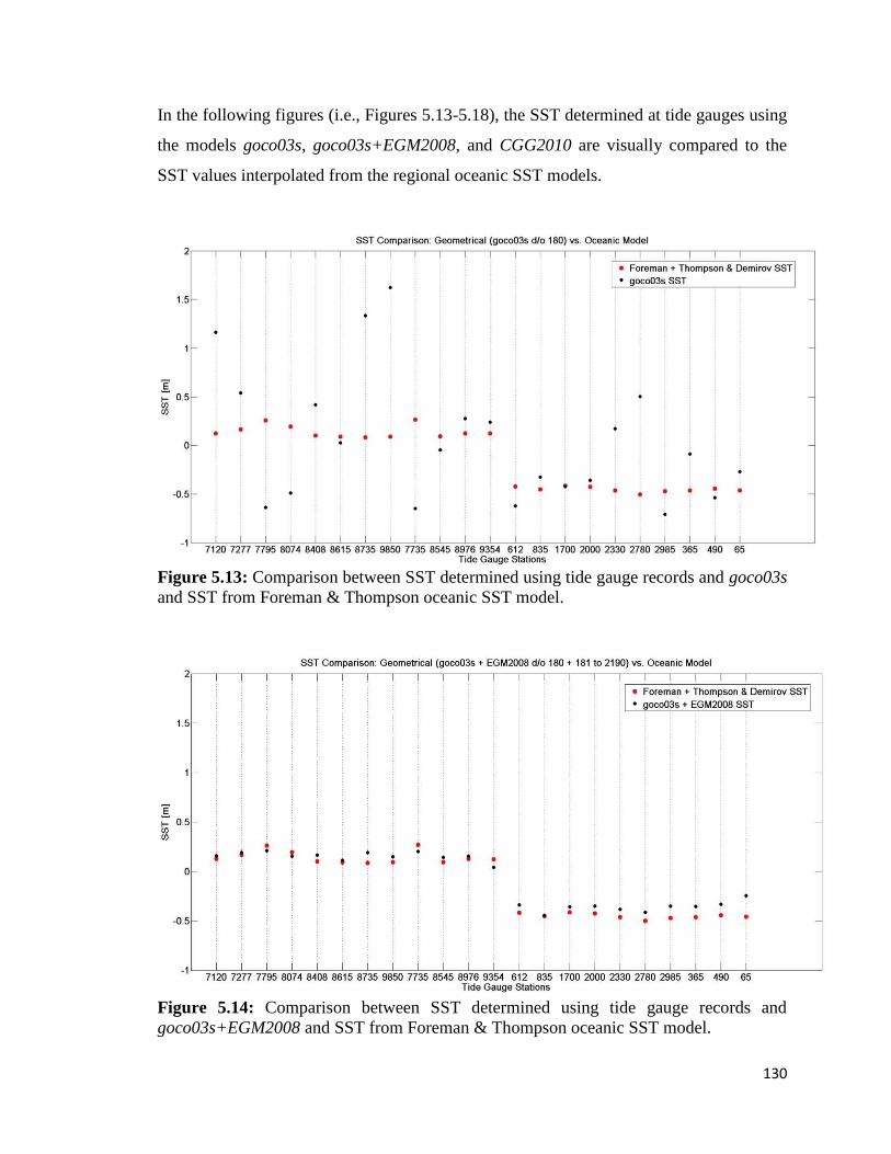
130
In the following figures (i.e., Figures 5.13-5.18), the SST determined at tide gauges using
the models goco03s, goco03s+EGM2008, and CGG2010 are visually compared to the
SST values interpolated from the regional oceanic SST models.
Figure 5.13: Comparison between SST determined using tide gauge records and goco03s
and SST from Foreman & Thompson oceanic SST model.
Figure 5.14: Comparison between SST determined using tide gauge records and
goco03s+EGM2008 and SST from Foreman & Thompson oceanic SST model.
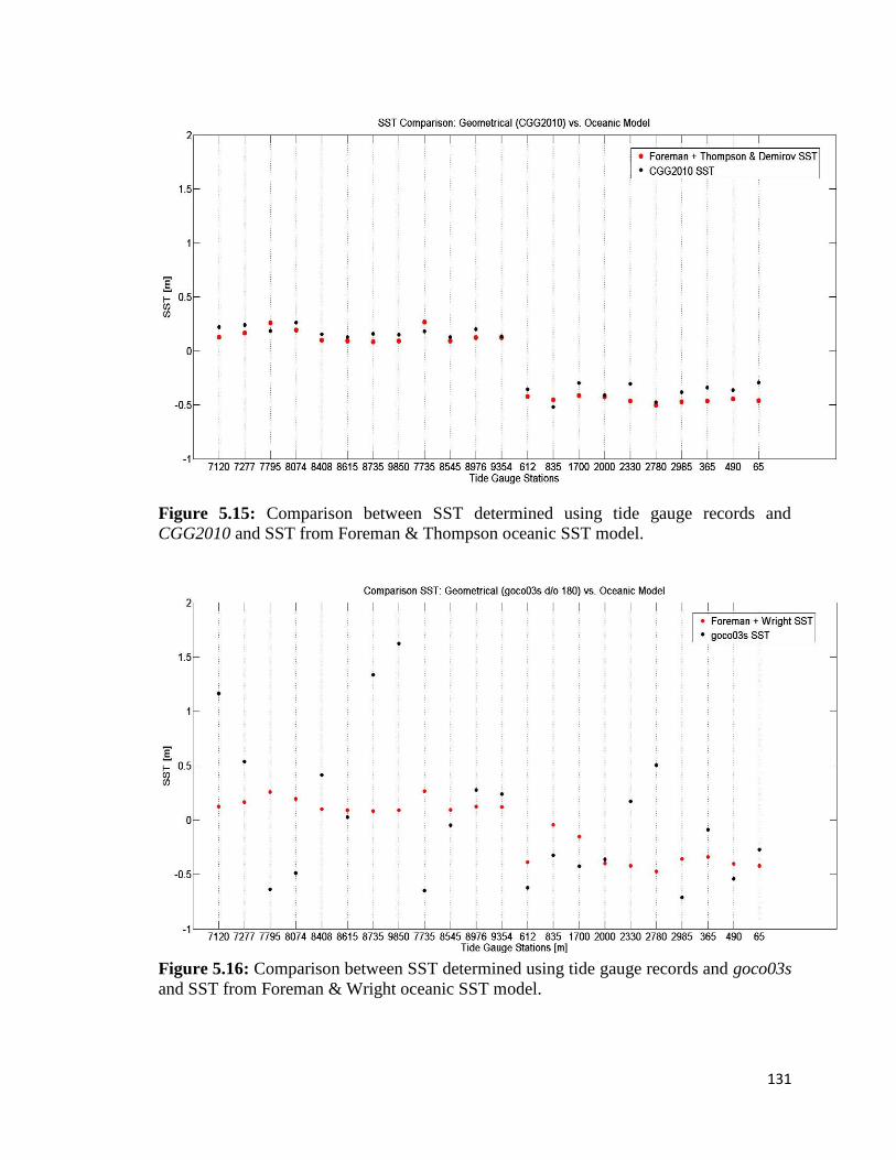
131
Figure 5.15: Comparison between SST determined using tide gauge records and
CGG2010 and SST from Foreman & Thompson oceanic SST model.
Figure 5.16: Comparison between SST determined using tide gauge records and goco03s
and SST from Foreman & Wright oceanic SST model.
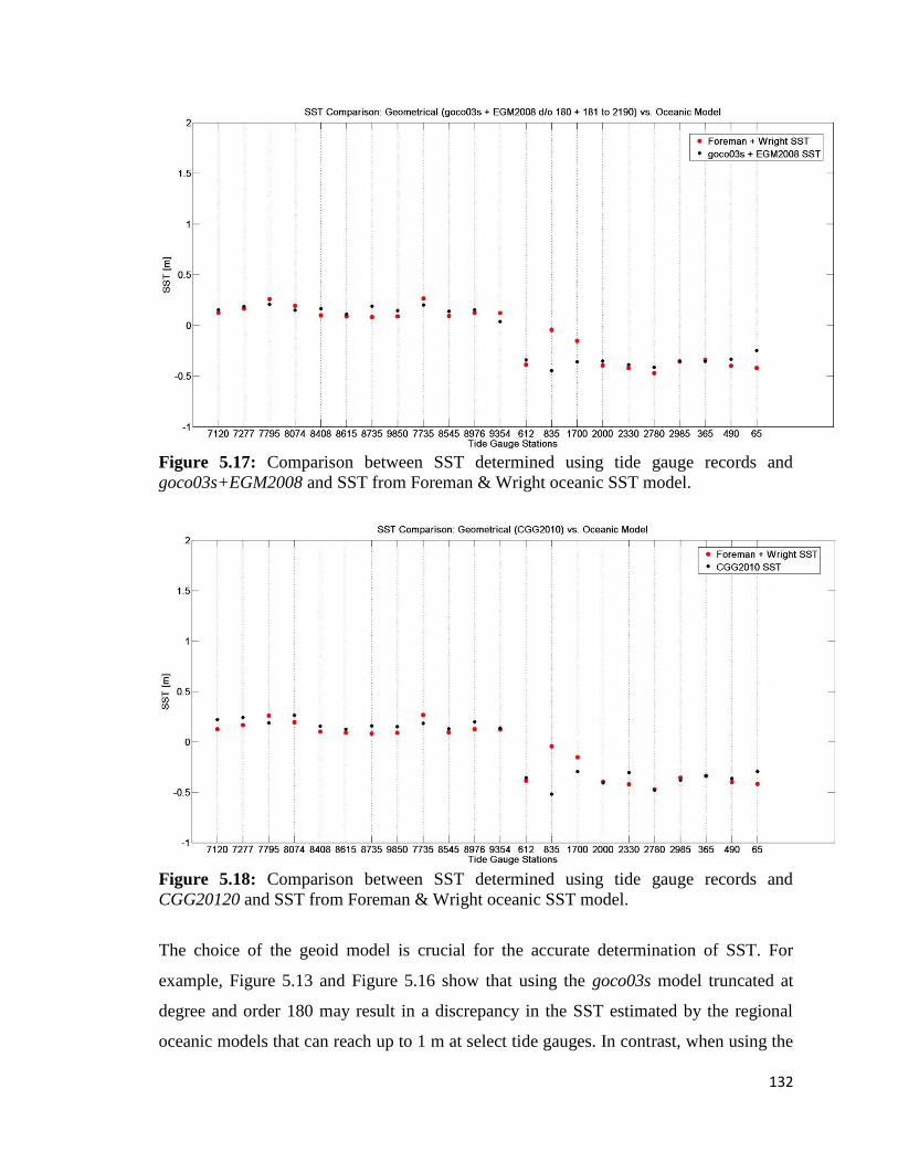
132
Figure 5.17: Comparison between SST determined using tide gauge records and
goco03s+EGM2008 and SST from Foreman & Wright oceanic SST model.
Figure 5.18: Comparison between SST determined using tide gauge records and
CGG20120 and SST from Foreman & Wright oceanic SST model.
The choice of the geoid model is crucial for the accurate determination of SST. For
example, Figure 5.13 and Figure 5.16 show that using the goco03s model truncated at
degree and order 180 may result in a discrepancy in the SST estimated by the regional
oceanic models that can reach up to 1 m at select tide gauges. In contrast, when using the
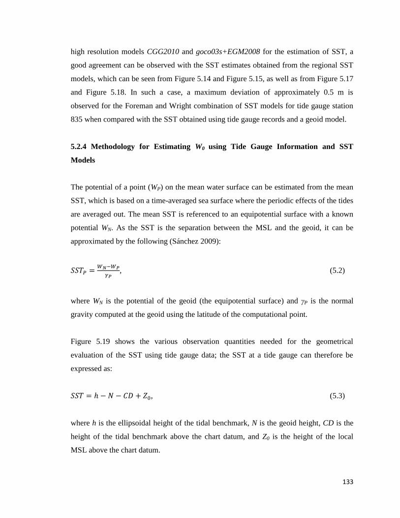
133
high resolution models CGG2010 and goco03s+EGM2008 for the estimation of SST, a
good agreement can be observed with the SST estimates obtained from the regional SST
models, which can be seen from Figure 5.14 and Figure 5.15, as well as from Figure 5.17
and Figure 5.18. In such a case, a maximum deviation of approximately 0.5 m is
observed for the Foreman and Wright combination of SST models for tide gauge station
835 when compared with the SST obtained using tide gauge records and a geoid model.
5.2.4 Methodology for Estimating W0 using Tide Gauge Information and SST
Models
The potential of a point (WP) on the mean water surface can be estimated from the mean
SST, which is based on a time-averaged sea surface where the periodic effects of the tides
are averaged out. The mean SST is referenced to an equipotential surface with a known
potential WN. As the SST is the separation between the MSL and the geoid, it can be
approximated by the following (Sánchez 2009):
, (5.2)
where WN is the potential of the geoid (the equipotential surface) and γP is the normal
gravity computed at the geoid using the latitude of the computational point.
Figure 5.19 shows the various observation quantities needed for the geometrical
evaluation of the SST using tide gauge data; the SST at a tide gauge can therefore be
expressed as:
, (5.3)
where h is the ellipsoidal height of the tidal benchmark, N is the geoid height, CD is the
height of the tidal benchmark above the chart datum, and Z0 is the height of the local
MSL above the chart datum.
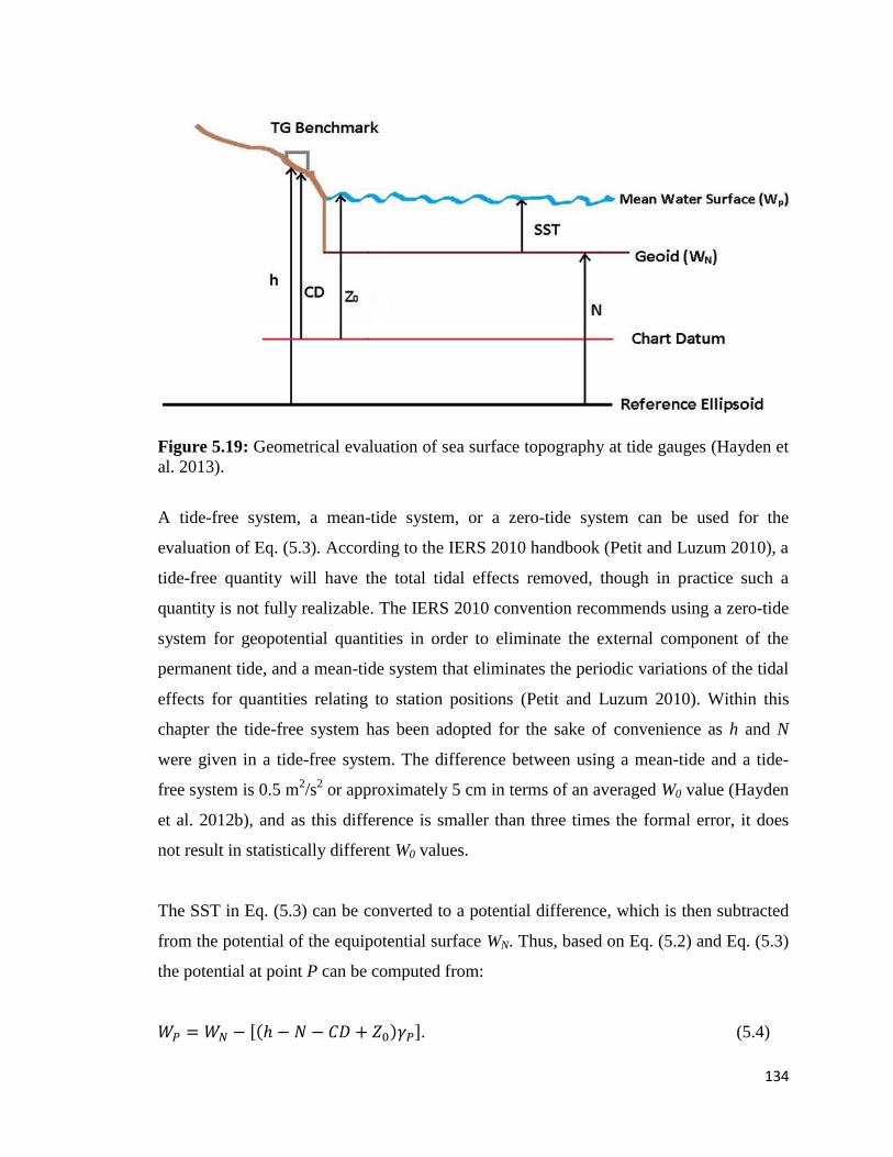
134
Figure 5.19: Geometrical evaluation of sea surface topography at tide gauges (Hayden et
al. 2013).
A tide-free system, a mean-tide system, or a zero-tide system can be used for the
evaluation of Eq. (5.3). According to the IERS 2010 handbook (Petit and Luzum 2010), a
tide-free quantity will have the total tidal effects removed, though in practice such a
quantity is not fully realizable. The IERS 2010 convention recommends using a zero-tide
system for geopotential quantities in order to eliminate the external component of the
permanent tide, and a mean-tide system that eliminates the periodic variations of the tidal
effects for quantities relating to station positions (Petit and Luzum 2010). Within this
chapter the tide-free system has been adopted for the sake of convenience as h and N
were given in a tide-free system. The difference between using a mean-tide and a tide-
free system is 0.5 m2/s
2 or approximately 5 cm in terms of an averaged W0 value (Hayden
et al. 2012b), and as this difference is smaller than three times the formal error, it does
not result in statistically different W0 values.
The SST in Eq. (5.3) can be converted to a potential difference, which is then subtracted
from the potential of the equipotential surface WN. Thus, based on Eq. (5.2) and Eq. (5.3)
the potential at point P can be computed from:
[ ]. (5.4)
135
The W0 value or the mean potential of the water surface is computed by means of the
least-squares solution of the system of observation equations evaluated by Eq. (5.4),
which for equally-weighted observations is simply the average of all the WP computed at
each tide gauge. It should be noted that Eq. (5.4) is used when evaluating the SST from
tide gauge data.
If one wants to evaluate WP using a SST model, then the following equation should be
used:
. (5.5)
For the sake of consistency, the SST models should be converted from a mean-tide
system to a tide-free system for the adequate comparison of the W0 values obtained from
tide gauges and those obtained using sea surface topography models. The tide-free value
SSTTF can be obtained using the conversion given in Eq. (5.6) below (Ekman 1989;
Mäkinen and Ihde 2009):
(( ) ), (5.6)
where SSTMT is the sea surface topography given in the mean-tide system, and φ is the
latitude of the SST node from the model.
The mean potential is obtained by a weighted average when W0 is evaluated from SST
models using:
∑
∑ , (5.7)
or
136
∑
∑
, (5.8)
where WPi is the potential of the water surface estimated from a SST node in the model,
and φi is the latitude of the SST node from the model. It should be noted that Eq. (5.7)
can only be considered an approximation as it does not comply with the Gauss-Listing
definition of the geoid (Gauss 1828; Bessel 1837; Listing 1873). The cosφi term in Eq.
(5.7) assigns less weight to higher latitude terms, which reflects the fact that SST
accuracy decreases with latitude as many SST models assimilate altimetry data. On the
other hand, Eq. (5.8) does comply with the Gauss-Listing definition (see Chapter 2,
Section 2.2). Then again, the use of either Eq. (5.7) or Eq. (5.8) yields essentially the
same W0 results; the difference is on the order of 0.01 m2/s
2, which equates to a 1 mm
error in SST (Hayden et al. 2012b).
It should also be noted that the tide gauges on the Atlantic coast located near the St.
Lawrence River may be affected by river discharge (Bourgault and Koutitonsky 1999). In
order to mitigate such effects, one may adjust the local MSL (i.e., Z0) for deep ocean
SST. The SST shown in Figure 5.19 is obtained from a SST model, and the difference
between the geometrical SST computed using geodetic data at the tide gauge and the SST
from a model results in the correction to be applied to Z0. In order to avoid SST values
near the coast, which are more likely to be erroneous due to the localized effects of the
coastline, an averaged oceanic SST at 50 km from the tide gauge location is used when
evaluating the correction to be applied to Z0. This is especially the case if the SST model
incorporates altimetry data such as the geodetic-based SST models presented in Section
5.2.3, since the altimetry signal is likely to be contaminated by the land portion of the
coastline. In this study the regional SST models are utilized for this correction as they
have better coverage when compared to the global models of ocean regions near the
coast. Additionally, the Foreman model is very dense in the coastal region when
compared with the global models, and is therefore less likely to be subject to
interpolation errors. The difference in W0 is at most 0.10 m2/s
2 or 1 cm when using a
137
correction from the regional SST models interpolated 50 km away from the tide gauges
or one that is interpolated to the tide gauge locations.
The values for h, CD, and Z0 were all brought to the same epoch of 2008.0. The
motivation for this comes from the fact that this study is part of the ESA STSE – GOCE+
“Height System Unification with GOCE” project, and in order to have consistency
among the various computations from the different research teams involved, the common
reference epoch of 2008.0 was chosen.
The ellipsoidal height h was originally given in ITRF 2005 epoch 2006.0 which was then
converted to ITRF 2008 epoch 2008.0 using software developed by NGS available at
http://www.ngs.noaa.gov/GEOID/GPSonBM09/. Corrections for vertical land motion
were also applied. The acceleration of the vertical motion is assumed to be zero and that
there is only a constant velocity difference:
(5.9)
where h2008.0 is the ellipsoidal height in ITRF 2008 epoch 2008.0 and VLM is the vertical
land motion velocity estimate. For the Pacific region, the vertical land motion rates are
mainly due to seismic variations, and these values were obtained from the GNSS-based
rates evaluated by Mazzotti et al. (2008). For the Atlantic and Arctic region, the vertical
land motion rates are primarily due to post-glacial rebound, and these values were
interpolated at the tide gauge locations from the Argus and Peltier (2010) GEODVEL1b
GPS solution
Similarly, CD and Z0 are adjusted by determining their epochs. The Z0 has an epoch of
2001.5, which is the average of the time series that ranges from 1992 to 2011. The CD
values have variable epochs which have been provided by the Canadian Hydrographic
Service. For the Pacific region, the CHS did not have epoch information for the chart
datum, so the CD values were left as originally given in the data files obtained by
NRCan. Furthermore, the CHS did not have complete epoch information for the chart
138
datum in the Atlantic region, thus the epoch information of the nearest available tide
gauge was utilized if this information was missing for a particular station. In order to
bring the epoch of all the CD and Z0 values to 2008.0, both sea level rise and vertical land
motion had to be taken into account.
The vertical land motion rate was applied with the following manner to Z0:
∑
(5.10)
and the sea level rise as
(5.11)
where nn a is the yearly is averaged water level time series and s a r s is the rate of
the sea level rise. The absolute sea level rate used was the 20th
century average for North
America: 1.8 mm/yr ±0.2 mm/yr (Church et al. 2004; Snay et al. 2007; Mazzotti et al.
2008).
Similarly for the CD values the following equation was used in order to bring the values
to epoch 2008.0:
( ) ( )
(5.12)
where och
is the epoch of the chart datum.
On a final note, it should be mentioned that corrections given in Eq. (5.9) to Eq. (5.12) do
not have a significant effect on W0, since the velocity corrections are of the order of
mm/year and thus they add only a few millimetres to h, CD, and Z0 (Rangelova et al.
2012).

139
5.3 Results and Discussion
5.3.1 W0 Evaluation with Tide Gauges and GOCE GGMs
In the ideal case, considering that the W0 is a single averaged value mainly dependent on
low-frequency spectral content, the effect of the GOCE omission error is not expected to
be significant. However, as previously shown in Section 5.2.3, the effect of the GOCE
omission error can be significant at selected tide gauges, and will not average out over the
limited number of gauges available for Canada. In Table 5.3, W0 results for the Pacific
and Atlantic regions with full 19 years of water level data are presented in order to
compare the results with those computed using the various SST models. As the regional
SST models are of variable density, in particular the Foreman model, they may cause the
W0 values to be biased as there are more SST nodes in Pacific than for the regional
models in the Atlantic, thus the W0 of the Pacific and Atlantic are examined separately
using goco03s in Table 5.3. The standard deviations are estimated by the a-posteriori
variance factor of the adjustment of Eq. (5.4) using a unit weight matrix; thus the error
estimates shown in the tables indicate a formal statistical accuracy.
Table 5.3: W0 values for Pacific and Atlantic tide gauges with 19 years of water level
data with GGMs expanded to degree and order 180 and 2,190 (add 62,636,800.00 m2/s
2
to values in table).
GGM Model Pacific Atlantic
goco03s
nmax:180
52.59 ± 2.13 58.30 ± 1.16
goco03s+EGM2008
nmax:180+181 to 2190
54.18 ± 0.13 59.21 ± 0.16
It can be observed from Table 5.3 that for the result with the extended
goco03s+EGM2008 model, the mean W0 is close to 62636854.00 m2/s
2 for the Pacific
and 62636859.00 m2/s
2 for the Atlantic. The potential decreases in the Pacific since the
SST for this region is mostly positive, which is also verified by the SST models for this
region as shown in Section 5.2.3. For the Atlantic region, the SST is for the most part
negative, thus it is reasonable for the potential to increase with respect to the WN surface

140
used in Eq. (5.4). For the Pacific region, the effect of the omission error on the W0 value
averages to 1.59 m2/s
2 or approximately a 16 cm difference when the satellite only model
is compared with the spectrally enhanced model. For the Atlantic region the effect of the
omission error averages to 0.92 m2/s
2 (or 9 cm).
Table 5.4: W0 values evaluated using Pacific and Atlantic tide gauges with 19 years of
water level data and different gravity field models (add 62,636,800.00 m2/s
2 to values in
the table).
Gravity Field Model Expanded to
Degree and Order nmax
W0 using Z0
without
Correction (m
2/s
2)
W0 using
Foreman and
Wright
Corrected Z0 (m
2/s
2)
W0 using
Foreman and
Thompson &
Demirov
Corrected Z0 (m
2/s
2)
goco03s
nmax
: 180
55.50 ± 1.39 55.52 ± 1.38 56.03 ± 1.43
goco03s+EGM2008
nmax
: 180+181 to 2190
56.78 ± 0.56 56.81 ± 0.56 57.31 ± 0.65
go_cons_gcf_2_tim_r4
nmax
: 200
55.23 ± 1.14 55.25 ± 1.14 55.76 ± 1.20
go_cons_gcf_2_tim_r4+EGM2008
nmax
: 200+201 to 2190
56.64 ± 0.55 56.66 ± 0.56 57.17 ± 0.64
go_cons_gcf_2_tim_r4
nmax
: 250
56.43 ± 0.97 56.45 ± 0.95 56.96 ±1.01
go_cons_gcf_2_tim_r4
nmax
: 250 (with error info)
56.55 ± 0.95 56.57 ±0.94 57.09 ± 1.00
go_cons_gcf_2_tim_r4+EGM2008
nmax
: 250+251 to 2190
56.60 ± 0.62 56.63 ± 0.65 57.14 ± 0.71
go_cons_gcf_2_dir_r4
nmax
: 210
55.46 ± 1.11 55.49 ± 1.11 55.99 ± 1.16
go_cons_gcf_2_dir_r4+EGM2008
nmax
: 210+2111 to 2190
56.68 ± 0.57 56.70 ± 0.57 57.21 ± 0.65
CGG2010 56.71 ± 0.60 56.74 ± 0.59 57.24 ± 0.69
141
Table 5.4 shows W0 values obtained using Z0 that has been corrected for deep ocean SST
using the regional SST models. Again, the effect of the GOCE model omission error on
the W0 value reaches approximately 1.30 m2/s
2 (or 13 cm) when using a combination of
Pacific and Atlantic tide gauges.
The effect of the omission error on W0 when using tim_r4 expanded to the maximum
available degree and order of 250 is approximately 2 cm when no error information is
utilized and less than 1 cm when error information is utilized. The error estimates utilized
may yield an overly positive estimate of the actual effect as no readily available error
information was available for the h, CD, and Z0 values, thus constant error values were
assumed (i.e., 2 cm, 5 cm, and 1 cm, respectively), and only the variances of the tim_r4
model was utilized for the propagation of the errors to the geoid height. In actuality, the
errors of the h, CD, and Z0 values could be larger.
Correcting Z0 for the SST of the deep ocean has an effect that is less than 1 cm when
utilizing the Wright SST model. On the other hand, the contribution of this correction is
approximately 5 cm when utilizing the Thompson & Demirov SST model. Thus, the
variability between SST models can be an appreciable factor in W0 estimation when only
a small number of tide gauges are available.
5.3.2 W0 Evaluation with Tide Gauges and Gravimetric Geoid Models
In this section, results for W0 evaluated with Eq. (5.4) using geoid undulations obtained
from regional gravimetric geoid models are presented. As both the CGG2010 and Ince et
al. (2012) gravimetric geoid models use the same terrestrial data to model the high
frequency contributions of the gravity field, it is expected that they will perform similarly
when evaluating W0. Likewise, gravimetric geoid models are also expected to perform
consistently with the spectrally enhanced GOCE+EGM2008 models presented in the
previous section. Hence, the gravimetric geoid models in this section provide another
measure of the difference in performance of the GOCE only models and that of the high
resolution gravity models when evaluating W0 from tide gauge averaging.

142
The results from Table 5.5 are consistent with those results utilizing the spectrally
enhanced GOCE models with EGM2008 shown in Table 5.4. This is expected as the
EGM2008 model also utilizes the same terrestrial data used to construct the CGG2010
and Ince et al. (2012) gravimetric geoid models in order to account for medium to short
wavelength contributions of the gravity field (Pavlis et al. 2012). The results computed
using the gravimetric geoid models help to further highlight the fact that simply utilizing
the GOCE models truncated at degree and order 180, 200, or 210 is not sufficient for
determining W0 from tide gauge averaging as the omission error affecting the SST and in
turn the potential at each tide gauge could be large, which will affect the W0
determination due to sparsely distributed and limited number of available tide gauges.
Table 5.5: W0 values for three Canadian regions computed with regional gravimetric
geoid models (add 62,636,800.00 m2/s
2 to all values).
Geoid Model CGG2010 Ince et al. (2012)
Pacific tide gauges with 19 years of water level data
Mean W0 (m2/s
2) 54.25 ± 0.13 54.17 ± 0.11
Atlantic tide gauges with 19 years of water level data
Mean W0 (m2/s
2) 59.67 ± 0.23 59.60 ± 0.19
All Arctic tide gauge stations (5 Stations)
Mean W0 (m2/s
2) 60.15 ± 0.17 60.19 ± 0.28
Pacific and Atlantic tide gauges with 19 years of water level data
Mean W0 (m2/s
2) 56.71 ± 0.60 56.64 ± 0.60
Pacific and Atlantic tide gauges with 19 years of water level data + All Arctic tide gauges
Mean W0 (m2/s
2) 57.35 ± 0.56 57.30 ± 0.56
All tide gauges (38 Stations)
Mean W0 (m2/s
2) 57.44 ± 0.47 57.38 ± 0.46
The W0 values estimated using CGG2010 and Ince’s model can be considered statistically
similar as the differences in the W0 values range from 0.04 m2/s
2 to 0.08 m
2/s
2, which is
well within the range of three times their formal errors that vary from 0.3 m2/s
2 to 0.8
m2/s
2. For example, the W0 value computed using CGG2010 for the Pacific region is
62636854.25 m2/s
2 while for the Atlantic region it is 62636859.67 m
2/s
2, and for the
Arctic region the W0 value averages to 62636860.15 m2/s
2. When utilizing the model
developed by Ince et al. (2012) the W0 value for the Pacific is 62636854.17 m2/s
2, for the
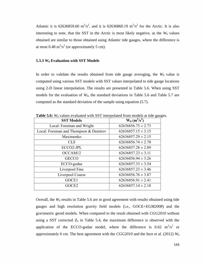
143
Atlantic it is 62636859.60 m2/s
2, and it is 62636860.19 m
2/s
2 for the Arctic. It is also
interesting to note, that the SST in the Arctic is most likely negative, as the W0 values
obtained are similar to those obtained using Atlantic tide gauges, where the difference is
at most 0.48 m2/s
2 (or approximately 5 cm).
5.3.3 W0 Evaluation with SST Models
In order to validate the results obtained from tide gauge averaging, the W0 value is
computed using various SST models with SST values interpolated to tide gauge locations
using 2-D linear interpolation. The results are presented in Table 5.6. When using SST
models for the evaluation of W0, the standard deviations in Table 5.6 and Table 5.7 are
computed as the standard deviation of the sample using equation (5.7).
Table 5.6: W0 values evaluated with SST interpolated from models at tide gauges.
SST Models W0 (m2/s
2)
Local: Foreman and Wright 62636856.75 ± 2.73
Local: Foreman and Thompson & Demirov 62636857.15 ± 3.15
Maximenko 62636857.29 ± 2.15
CLS 62636856.74 ± 2.70
ECCO2-JPL 62636857.28 ± 2.89
OCCAM12 62636857.23 ± 3.11
GECCO 62636856.94 ± 3.26
ECCO-godae 62636857.33 ± 3.54
Liverpool Fine 62636857.23 ± 3.46
Liverpool Coarse 62636856.76 ± 3.87
GOCE1 62636856.91 ± 2.41
GOCE2 62636857.14 ± 2.18
Overall, the W0 results in Table 5.6 are in good agreement with results obtained using tide
gauges and high resolution gravity field models (i.e., GOCE+EGM2008) and the
gravimetric geoid models. When compared to the result obtained with CGG2010 without
using a SST corrected Z0 in Table 5.4, the maximum difference is observed with the
application of the ECCO-godae model, where the difference is 0.62 m2/s
2 or
approximately 6 cm. The best agreement with the CGG2010 and the Ince et al. (2012) W0
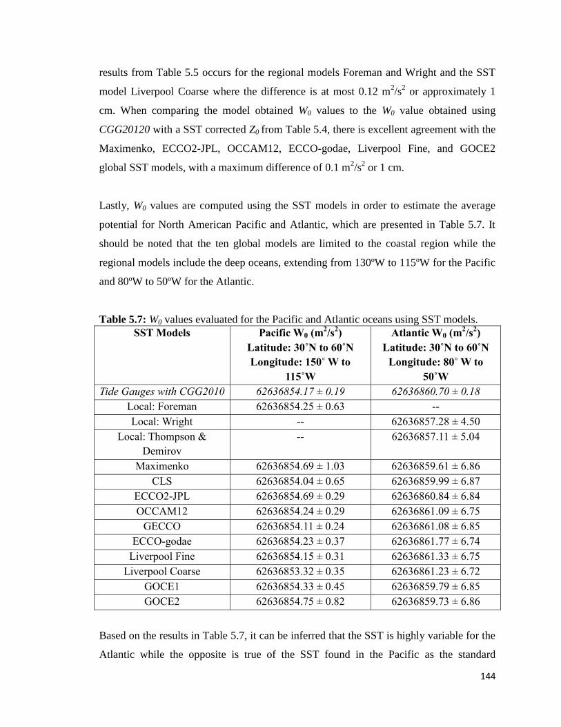
144
results from Table 5.5 occurs for the regional models Foreman and Wright and the SST
model Liverpool Coarse where the difference is at most 0.12 m2/s
2 or approximately 1
cm. When comparing the model obtained W0 values to the W0 value obtained using
CGG20120 with a SST corrected Z0 from Table 5.4, there is excellent agreement with the
Maximenko, ECCO2-JPL, OCCAM12, ECCO-godae, Liverpool Fine, and GOCE2
global SST models, with a maximum difference of 0.1 m2/s
2 or 1 cm.
Lastly, W0 values are computed using the SST models in order to estimate the average
potential for North American Pacific and Atlantic, which are presented in Table 5.7. It
should be noted that the ten global models are limited to the coastal region while the
regional models include the deep oceans, extending from 130ºW to 115ºW for the Pacific
and 80ºW to 50ºW for the Atlantic.
Table 5.7: W0 values evaluated for the Pacific and Atlantic oceans using SST models.
SST Models Pacific W0 (m2/s
2)
Latitude: 30˚N to 60˚N
Longitude: 150˚ W to
115˚W
Atlantic W0 (m2/s
2)
Latitude: 30˚N to 60˚N
Longitude: 80˚ W to
50˚W
T d a g s w th 2 62636854 7 ± 9 6263686 7 ± 8
Local: Foreman 62636854.25 ± 0.63 --
Local: Wright -- 62636857.28 ± 4.50
Local: Thompson &
Demirov
-- 62636857.11 ± 5.04
Maximenko 62636854.69 ± 1.03 62636859.61 ± 6.86
CLS 62636854.04 ± 0.65 62636859.99 ± 6.87
ECCO2-JPL 62636854.69 ± 0.29 62636860.84 ± 6.84
OCCAM12 62636854.24 ± 0.29 62636861.09 ± 6.75
GECCO 62636854.11 ± 0.24 62636861.08 ± 6.85
ECCO-godae 62636854.23 ± 0.37 62636861.77 ± 6.74
Liverpool Fine 62636854.15 ± 0.31 62636861.33 ± 6.75
Liverpool Coarse 62636853.32 ± 0.35 62636861.23 ± 6.72
GOCE1 62636854.33 ± 0.45 62636859.79 ± 6.85
GOCE2 62636854.75 ± 0.82 62636859.73 ± 6.86
Based on the results in Table 5.7, it can be inferred that the SST is highly variable for the
Atlantic while the opposite is true of the SST found in the Pacific as the standard

145
deviations for the Atlantic range from 4.50 m2/s
2 to 6.86 m
2/s
2 while the standard
deviation for the Pacific ranges from 0.24 m2/s
2 to 1.03 m
2/s
2 with the use of the different
SST models. The MSL of the Pacific is approximately 20 cm above the global
conventional W0 value 62636856.00 m2/s
2 adopted by the IERS 2010 (Petit and Luzum
2010) while the MSL of the Atlantic is approximately 40 cm below this surface. From
Table 5.7 it can be observed that the Thompson & Demirov and Wright SST models yield
a lower potential for the Atlantic when compared with the 10 other global SST models
because these two models include the deep ocean part of the South Atlantic where
warmer waters from the Gulf Stream create a positive SST (see Figure 5.2). For example,
the W0 value for the Atlantic using the Thompson & Demirov and Wright SST models is
62636857.11 m2/s
2 and 62636857.28 m
2/s
2, respectively. In contrast, for the global model
ECCO2-JPL the W0 value for the Atlantic is 62636860.84 m2/s
2, which represents a
maximum difference of 3.73 m2/s
2 (or 38 cm) when compared to the use of the regional
models.
Thus, when utilizing the regional SST models in the evaluation of W0 as an average over
North America, one expects a decrease in potential when compared to the Canadian case
as the SST values off the Canadian Atlantic coast are mostly negative. For example,
when using the Foreman + Wright SST model combination yields a W0 value of
62636855.77 m2/s
2 and the Foreman + Thompson & Demirov combination yields a W0
value of 62636855.68 m2/s
2 for North America.
5.4 Summary
The objectives of this chapter include the evaluation of W0 from tide gauge records and
geoid models within the context of realizing a new geoid-based and GNSS-accessible
vertical datum for Canada in order to replace the outdated CGVD28, and to validate the
results of tide gauge averaging utilizing SST models. One of the main goals was to assess
the performance of the GOCE-based GGMs for the purpose of estimating W0 in Canada
using tide gauges. This was done by evaluating the SST at tide gauges utilizing the
goco03s, tim_r4, and dir_r4 GOCE satellite-only models. Based on plots comparing the

146
SST values obtained from regional SST models with those obtained using goco03s and
tide gauge records, it was expected that the omission error of the GOCE-only models
would have a significant effect on the computed W0 value due to the small number of tide
gauges available on the Atlantic and Pacific coasts. In order to test this, the GOCE
models were spectrally extended with the high resolution gravity model EGM2008.
Furthermore, the performance of the GOCE only models for the estimation of W0 was
compared with that of two gravimetric geoid models.
It was shown that the effect of the GOCE omission error on W0 averages to 16 cm in the
Pacific and 9 cm in the Atlantic, and averages to 13 cm when both Pacific and Atlantic
tide gauges are utilized. Thus, it can be concluded that the truncation degree of the GOCE
models is important for W0 determination; in particular, the truncation degrees of 180-210
are not adequate when evaluating W0 from scattered tide gauge points in Canada as the
higher frequency contributions of the gravity field are not properly modeled. On the other
hand, it has been shown that when the GOCE tim_r4 model is expanded to its maximum
degree 250, the effect of the GOCE omission error on the estimation of W0 is between 1
to 2 cm. However, further investigation is needed in order to accurately quantify the
effects of the GOCE model commission errors and the measurement errors on the W0
value.
Thus, based on the results from Chapter 4 and this chapter, the effect of the GOCE
omission error on the averaged W0 is expected to be negligible for well distributed
stations, which also indicates that the use of a satellite-only GGM may be sufficient for
the computation of W0 in regions with very good coverage and distribution of tide gauge
or GNSS levelling benchmarks. Based on the results in this study, it is recommended that
a high resolution geoid model such as CGG2010 or EGM2008 should be used when
computing W0 by the tide gauge averaging method in order to adequately model the high
frequency components of the gravity field, in particular for regions with poor coverage
and distribution of tide gauges. On the other hand, it is recommended to use regional SST
models for the determination of W0 in North America, as they have the best agreement
with the geometrically determined SSTs and adequately reflect the positive SST of the
147
South Atlantic when compared with the global models. By extension of this reasoning,
the ECCO2-JPL global SST model can also be utilized.
It is expected that data gaps in the water level time series, missing epoch information for
the chart datums on both the Pacific and Atlantic coasts, interpolation errors for epoch
information for the chart datums, interpolation errors for determining post-glacial
rebound velocities at tide gauges, and utilizing MSL values that are based on time series
shorter than 19 years will affect the quality of the tide gauge data. However, in this study,
the effect of these limitations on the final MSL obtained from tide gauge data were not
investigated, and therefore may be considered for future investigations. The main factor
to consider is the interpolation error of the SSTs at the tide gauges locations when
validating the tide gauge averaging results with the use of SST models. Depending on the
assimilation of different data types in the SST model, such as the incorporation of
altimetry data, the quality of the SST values near the coast acquired from a model needs
to be carefully considered.
One needs to utilize a 19-year water level time series for the estimation of W0 of the local
MSL in order to average out the effects of the tides and the weather. Such a requirement
limits the number and the distribution of tide gauges available for determining W0 at the
Canadian coasts. Data gaps in the water level time series have been avoided by
interpolating values from neighbouring ones. At any rate, it is not expected that this will
significantly affect the W0 results since the MSL values have been averaged from daily to
monthly to annual, and finally to 19-year averages.
Furthermore, the height of the tidal benchmark CD will not be significantly affected due
to missing epoch information or interpolation errors, since when updating the epoch of
the chart datum to 2008.0, it is only a matter of a few millimetres to one centimetre
difference, and as such it will not have a significant effect on the final W0 value. This is
because the geoid is a smooth surface and W0 is obtained by averaging. Likewise, this
applies for interpolation errors of the post-glacial rebound rates where the annual

148
velocities are of the order of millimetre. Thus, the effect in the final W0 computation was
not significant.
The potentials obtained from tide gauge averaging in this chapter cannot be considered an
average for all of North America since U.S.A. tide gauges were not included in the study.
This limitation can be overcome by utilizing SST models to compute W0 instead of tide
gauges as a good agreement has been discerned between the SST estimated from tide
gauge data and the SST values obtained from models. The main factor for the consistency
between the SST values from models and those obtained using tide gauge information is
the use of an accurate and high resolution geoid model.
Moreover, the Arctic region lacks sufficient water level data and SST model coverage.
Therefore, SST values from this region cannot be included when estimating a continental
average for W0. Consequently, the W0 results presented within this chapter using tide
gauge averaging are primarily biased to the Pacific and Atlantic coasts in the southern
region of Canada.
Without the inclusion of Arctic SST values for the estimation of a North American W0
value, it can be discerned that the W0 values presented within this chapter are
coincidentally close to the standard IERS (2010) global value of 62636856.00 m2/s
2. In
other words, the W0 values presented within this chapter cannot be considered statistically
different from the IERS 2010 conventional value as the difference between these W0
values is less than three times their formal errors. The W0 values are visually summarized
in Figures 5.21 and 5.22. The main consequence of adopting the IERS 2010 W0 value for
the geoid-based and GNSS-accessible vertical datum that will replace CGVD28 in
Canada is that it represents an average over the entire North American continent;
subsequently it will not reflect the potential of the local MSL along the coasts in Canada
as illustrated in Figure 5.20. For example, in the Pacific, it may appear that some heights
are below the observable local mean sea level in that region.

149
Figure 5.20: Differences in local MSL between west and east coast of Canada with
respect to IERS (2010) W0 62636856.00 m2/s
2.
Lastly, it should be noted that climate-related changes will affect the MSL, due to factors
such as the addition of melt water from Greenland, Alaska glaciers, and Canadian ice
caps, and the possible expansion of the ocean due to warming of the ocean surface.
Consequently, these effects will influence the W0 value over a decade and longer.
However, since the adopted W0 value for North America is a conventional value, it does
not necessarily represent the exact value of the coastal mean sea level for North America.
Figure 5.21: Summary of W0 estimates using GOCE GGMs and tide gauge information.
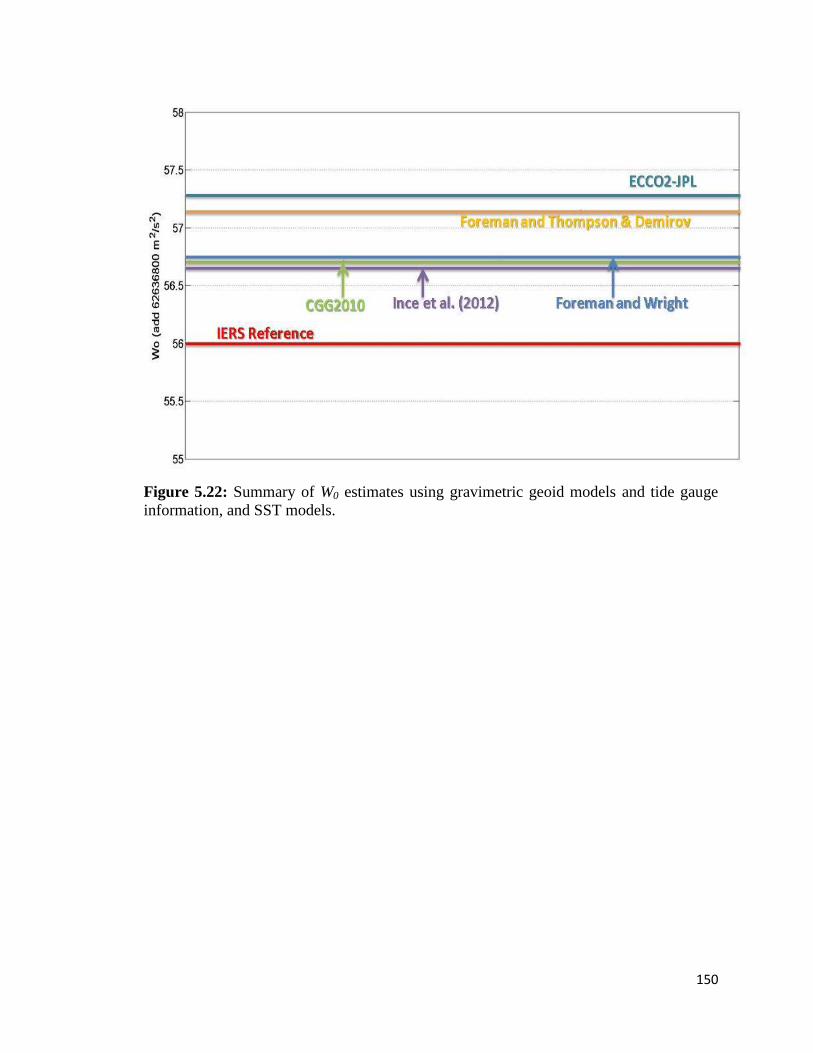
150
Figure 5.22: Summary of W0 estimates using gravimetric geoid models and tide gauge
information, and SST models.

151
CHAPTER 6
CONCLUSIONS
6.1 Thesis Statement
The main motivation of this thesis was to assess whether a GGM or a geoid model
constructed from satellite only observations is sufficient for geodetic applications such as
datum unification or the determination a conventional W0 value for a regional geoid-
based vertical datum, as these applications depend on a highly accurate and globally
consistent geoid or gravity field model. The use of a satellite only geopotential model
avoids the biases present in terrestrial data that is needed for gravimetric geoid modelling,
which has been essential for establishing accurate geoid models, since gravity and
topography data is needed to sufficiently model the high frequency contributions of the
gravity field. By the end of its lifespan, it is expected that the GOCE mission will achieve
a 1-2 cm geoid accuracy at a spatial resolution of approximately 100 km. In essence it
would then provide the long awaited satellite only geopotential models that will simplify
tasks such as datum unification and the establishment of a global height system. In order
to answer the question of whether a satellite-only gravity field model is sufficient for
datum unification and regional W0 determination in North America, the following topics
were investigated:
Evaluation of recently released satellite only global geopotential models with a
focus on GOCE-based models.
Estimation of local vertical datum offsets for classical levelling-based vertical
datums in North America for the purpose of datum unification using GOCE
satellite only models.
Estimation of W0 for the implementation of a geoid-based GNSS-accessible
vertical datum that will replace the outdated CGVD28 in Canada using regional
tide gauges and GOCE satellite only models, in addition to EGM2008 extended
GOCE models and gravimetric geoid models in order study the effect of the
GOCE model omission error on W0.
152
6.2 Conclusions
The following conclusions can be made from the GGM model evaluations:
GOCE satellite-only models have overall better agreement with independent
terrestrial data sets when compared to pre-GOCE era satellite (GRACE and
CHAMP) models
The agreement of GOCE models when compared with independent terrestrial
datasets improve as the time series of GOCE observations increases. The fourth
generation tim_r4 and dir_r4 have the best overall performance in North America,
which is expected due to the fact that these models contain a time series of GOCE
observations that is at least double the length of the previously released models.
GOCE satellite-only GGMs have good agreement with the independent
GNSS/levelling data up to the spectral band of harmonic degree 210 in North
America.
The fourth generation GOCE models tim_r4 and dir_r4 show improvement in the
higher spectral bands when compared with the third generation GOCE satellite-
only models.
Due to the increasing effect of the GOCE commission error above the spectral
band of harmonic degree 200-210, the GOCE only models are truncated at degree
and order 200-210 for the use in applications of estimating local vertical datum
offsets and W0.
The dir_r4 model, which contains a GRACE-based background model, has
achieved a 1.2 cm global geoid accuracy at degree and order 200, which satisfies
the GOCE mission objective of achieving 1-2 cm geoid accuracy at a spatial
resolution of approximately 100 km. With a longer time series of GOCE
observations, (i.e., fifth generation GOCE models) it is expected that the pure
GOCE model based on the time-wise approach may also achieve the GOCE
mission goals.
The following conclusions can be made from the estimation of local vertical datum
offsets for North American vertical datums using GOCE GGMs:
153
The effect of the GOCE model omission error on LVD offsets when using
Canadian GNSS/levelling benchmarks and fourth generation GOCE models is 8
cm. The effect of the GOCE model omission error on the LVD offset estimate is
2-3 cm when using the U.S.A. GNSS/levelling data. This difference is attributed
to the respective configuration and density of the GNSS/levelling benchmarks
available in each respective country.
The effect of the GOCE omission error on the estimation of the local vertical
datum offset is amplified for regions with rough topography, sparse/irregular
GNSS/levelling benchmark configuration, and limited number of benchmarks/tide
gauges, especially in relation to the total size of the test network. Due to this, a
GOCE-based model should be used in a remove-compute-restore scheme with
gravity and terrain data in order to rigorously model the higher frequency
contributions of the gravity field.
GOCE commission error and the measurement errors of the GNSS and levelling
data need to be taken into account, in particular for regions with limited
geographic coverage, when estimating local vertical datum offsets as the effect on
the LVD offset estimate can reach the dm-level.
The spatial tilts found in the Canadian Nov07 and NAVD88 networks, and the
U.S.A. NAVD88 network can be modelled with a 2-parameter corrector term
model. The model parameters may be estimated simultaneously with the LVD
offset estimates or the spatial tilts may be removed before the least-squares
estimation of the LVD offset, as the effect on the LVD offset estimate is at most 1
cm.
The following conclusions regarding the estimation of W0 using GOCE GGMs and tide
gauge information can be made:
GOCE satellite only models truncated at degree and order 180 are not sufficient
for estimating accurate SST values using geodetic information at tide gauges.
Differences between SST values obtained from regional SST models and those
obtained using GOCE satellite only models truncated at degree and order 180 can
reach up to 1 m.
154
GOCE satellite only models truncated at degree and order 180, 200, and 210 are
not sufficient for W0 estimation when a limited number of tide gauges are
available; the effect of the GOCE omission error on the W0 value is at the dm-
level when compared with W0 estimates obtained with gravimetric geoid models
and the ultra-high resolution GGM EGM2008.
SST models validate the W0 results obtained using tide gauge records and
gravimetric geoid and high resolution gravity field models.
In addition to tide gauge averaging, the regional SST models can be used to
estimate W0 for North America.
In conclusion, a satellite only geopotential model that can accurately model the geoid
signal in regions where less than ideal conditions and datasets are the reality is not
currently available. Thus, it is recommended that GOCE GGMs be rigorously combined
with gravity and topography data, if such data sets are available.
6.3 Recommendations
In order to accurately compute LVD offsets the following are recommended:
Removal of spatial tilts preferably before the estimation of the LVD offset in
order to avoid the inseparability between the LVD offset term and the bias
parameters of the corrector term model. If one wants to estimate the spatial tilts
and the LVD offsets simultaneously in the least-squares adjustment, the choice of
the parametric model needs to be carefully considered (see, e.g., Kotsakis et al.
2011). Moreover, the testing of various parametric models may be necessary to
determine which corrector term model will most effectively remove the
systematic errors found within the levelling network (see, e.g., Fotopoulos 2003).
Inclusion of error information for the ellipsoidal, orthometric, and geoid heights if
this data is available. This is especially important for test networks with a limited
geographic coverage as the commission error of the GGM for wavelengths that
exceed the size of the test area may act as a bias on the LVD offset estimate.
155
The use of a high resolution geoid model that incorporates local gravity and
terrain data is recommended in order to adequately model the effect of the GGM
omission error. In such a case, the GOCE-based dir_r4 model may be used in a
remove-compute-restore scheme for geoid modelling as outlined in Chapter 2
Section 2.6 as it will contribute to the long to medium wavelengths of the gravity
field signal.
The methodology presented in Chapter 4 Section 4.2 may be utilized for LVD
offset computations.
The estimation of W0 can be achieved using tide gauge data or using SST models. If
using tide gauge averaging method to compute W0 the following are recommended:
Evaluate the 19-year average MSL at tide gauges using tide gauges that have long
term water level records without significant data gaps (i.e., no more than 2-3 years
of missing water level data).
Bring h, CD, and Z0 in Eq. (5.4) to the same epoch by accounting for vertical land
motion and sea level rise using Eq. (5.9), Eq. (5.11), and Eq. (5.12).
Correct Z0 using deep ocean SST using SST models in order to mitigate effects of
river discharge at tide gauges. For North America, the use of regional SST models
(i.e., Foreman, Wright, and Thompson & Demirov) is recommended.
Use of a high resolution geoid model (e.g., GOCE+EGM2008, EGM2008,
USGG2012, CGG2010, or Ince et al. (2012)) in order to accurately estimate the
SST of the mean water level at a tide gauge. Ideally, a gravimetric geoid model
that utilizes the fourth generation GOCE GGMs is preferable.
Estimate W0 by the means of the least-square solution of the system of
observation equations evaluated by Eq. (5.4). If accuracy information for h, CD,
Z0, and N are available then they can be included.
If using SST models for W0 determination in North America the following are
recommended:
Use of regional SST models (i.e., Foreman, Wright, and Thompson & Demirov)
and ECCO2-JPL global model due to best agreement with geometrical SST
156
evaluated at tide gauges. Regional models have good coastal and deep ocean
coverage.
Use of Eq. (5.8) to estimate W0 as it complies with the Gauss-Listing definition of
the geoid.
6.4 Future Investigations
There are other investigations that can be conducted in order to further study the
limitations and benefits of the GOCE satellite-only GGMs for a variety of geodetic
applications:
GOCE models can be evaluated with other types of independent terrestrial
datasets, such as, e.g., astro-geodetic deflections and SST, other than
GNSS/levelling benchmarks. Again, comparisons are only valid if the reliability
of the terrestrial datasets is good. Also, one may also include the effect of the
residual terrain signal and parameterize systematic effects that might be present in
the terrestrial data when conducting a GGM evaluation.
For applications such as estimating local vertical datum offsets, one should ideally
propagate the GOCE commission errors using a fully populated variance-
covariance matrix. This is not a trivial task as it requires the inversion of
computationally demanding matrices; studies such as Gerlach and Fecher (2012)
have investigated how to make this task more feasible. As well, the errors of
gravity/topographic data, and that of the control data (i.e., ellipsoidal and
orthometric heights from GNSS and levelling) should be included.
One may also investigate the temporal effects such as rising sea level due to
climate change on the determination of SST and in turn W0 determination.
GOCE models can be utilized in gravimetric geoid modelling, for applications
such as the implementation of a regional geoid-based vertical datum, in order to
see if there is improvement with respect to past gravimetric geoid models that
have not utilized recently released GOCE models for long to medium wavelength
contributions of the gravity field.
157
And, lastly, further investigations into the systematic errors of the CGVD28 network may
be necessary, as the parametric models used within this study may not be adequate to
model the more complex systematic errors and distortions present within the CGVD28
network.
158
REFERENCES
Altamimi Z., Sillard P. and Boucher C., 2007, ITRF2005 A new release of the
International Terrestrial Reference Frame, J. Geophys. Res., 112, doi:
10.1029/2007JB004949.
Anderson O.B. and Knudsen P., 2009, DNSC08 mean sea surface and mean dynamics
topography models, J Geophys. Res., 114, C11001, DOI: 10.1029/2008JC005179.
Ardalan A., Grafarend E. and Kakkuri J., 2002, National height datum, the Gauss-Listing
geoid level value w0 and its time variation w0 (Baltic Sea Level Project: epochs 1990.8,
1993.8, 1997.4), J Geod., 76, 1-28.
Argus D.E. and Peltier W.R., 2010, Constraining models of postglacial rebound using
space geodesy: a detailed assessment of model ICE-5G (VM2) and its relatives, Geophys.
J. Int., 181, 697-723.
Balasubramania N., 1994, Definition and realization of the global vertical datum, OSU
Report No. 427, The Ohio State University, Columbus, U.S.A.
Bessel F.W., 1837, Über den Einfluss der Unregelmässigkeiten der Figur der Erde auf
geodätische Arbeiten und ihre Vergleichung mit den Astronomischen Bestimmungen,
Astronomische Nachrichten, 14, 269.
Biancale R., Balmino G., Lemoine J-M.,.Marty J-C., Moynot B., Barlier F., Exertier P.,
Laurain O., Gegout P., Schwintzer P., Reigber C., Bode A., Gruber T., König
R.,Massmann F-H., Raimondo J.C., Schmidt R. and Zhu S.Y., 2000, A new global
Earth’s gravity field model from satellite orbit perturbations: GRIM5-S1, Geophys. Res.
Lett., 27, 22, 3611–3614.
159
Bingham R. and Haines K., 2006, Mean dynamic topography: Intercomparisons and
errors, Philos. Trans. R. Soc., Ser. A., 264, 903-916.
Bingham R.J., Haines K. and Hughes C.W., 2008, Calculating the ocean’s mean dynamic
topography from a Mean Sea Surface and a Geoid, J Atmos. Ocean. Tech., 25, 1808-
1822.
Bolkas D., Fotopoulos G. and Sideris M.G., 2012, Referencing regional geoid-based
vertical datums to national tide gauge networks, J Geod. Sci., 2, 4, 363-369.
Bourgault D. and Koutitonsky V.G., 1999, Real-time monitoring of the freshwater
discharge at the head of the St. Lawrence Estuary, Atmosphere-Ocean 37, 2, 203-220.
Burša M., Kouba J., Raděj K., True S.A., Vatrt V. and Vojtíšková M., 1998, Mean
Earth’s Equipotential Surface from TOPEX/POSEIDON Altimetry, Studia Geoph. et
Geod., 42, 459-466.
Burša M., Kenyon S., Kouba J., Šima Z., Vatrt V. and Vojitišková M., 2004, A global
vertical reference frame based on four regional vertical datums, Stud. Geophys. Geod.,
48, 493-502.
Bruinsma S.L., Marty J.C., Balmino G., Biancale R., Foerste C., Abrikosov O. and
Neumayer H., 2010, GOCE Gravity Field Recovery by Means of the Direct Numerical
Method, Proceeding at the ESA Living Planet Symposium, 27th June - 2nd July 2010,
Bergen, Norway; See also: earth.esa.int/GOCE.
Church J.A., White N.J., Coleman R., Lambeck K. and Mitrovica J., 2004, Estimates of
the regional distribution of sea level rise over the 1950-2000 period, J Clim., 17, 2609-
2625.

160
Colombo O.L., 1980, A world vertical network, OSU Report No. 296, The Ohio State
University, Columbus, U.S.A.
Craymer M.R. and Lapelle E., 1997, The GPS Supernet: An Integration of GPS Projects
Across Canada, Internal Report, Geodetic Survey Division, Natural Resources Canada,
Ottawa, Canada.
CVRS Conventions, 2007, Conventions for the Definition and Realization of a
Conventional Vertical Reference System (CVRS), IAG Inter-Commission Project, ICP
1.2 Vertical Reference Frames.
Dayoub N., Edwards S.J. and Moore P., 2012, The Gauss-Listing geopotential value W0
and its rate from altimetric mean sea level and GRACE, J Geod., 86, 9, 681-694.
Drinkwater M.R., Floberghagen R., Haagmans R., Muzi D. and Popescu A., 2003, VII:
Closing Session: GOCE: ESA’s First Earth Explorer Core Mission, Space Sci. Rev., 108,
1-2, 419-432.
Ekman M., 1989, Impacts of geodynamic phenomena on systems for height and gravity,
Bull. Geod., 63, 281-296.
Ekman M. and Mäkinen J., 1996, Mean sea surface topography in the Baltic Sea and its
transition area to the North Sea: a geodetic solution and comparison with oceanographic
models, J Geophys. Res., 101, C5, 11993-11.
Entin I.I., 1959, Main Systematic Errors in Precise Levelling, Bull. Geoid., 52, 1, 37-45.
Foreman M.G.G., Crawford W.R., Cherniawsky J.Y. and Galbraith J., 2008, Dynamic
ocean topography for the northeast Pacific and its continental margins, Geophys. Res.
Letters, 35, L22606, DOI: 10.1029/2008GL035152.
161
Forsberg R., and Tscherning C., 1981, The use of height data in gravity field
approximations by collocation, J. Geophys. Res., 86, B9, 7843-7854.
Forsberg R., 1984, A study of terrain reductions, density anomalies and geophysical
inversion methods in gravity field modelling, OSU Report No. 355, Department of
Geodetic Science and Surveying, Ohio State University, Columbus, U.S.A.
Forsberg R., 1985, Gravity field terrain effect computations by FFT, Bull. Geod., 59, 4,
342-360, doi: 10.1007/BF02521068.
Förste C.H., Flechtner F., Schmidt R., Stubenvoll R., Rothacher M., Kusche J.,
Neumayer H., Biancale R., Lemoine J.M. , Barthelmes F., Bruinsma S., König R. and
Meyer U.L., 2008, EIGEN-GL05C - A new global combined high-resolution GRACE-
based gravity field model of the GFZ-GRGS cooperation, Geophysical Research
Abstracts, Vol. 10, EGU2008-A-03426, 2008, EGU General Assembly 2008.
Förste C., Stubenvoll R., König R., Raimondo J., Flechtner F., Barthelmes F., Kusche J.,
Dahle C., Neumayer H., Biancale R., Lemoine J. and Bruinsma S., 2009, Evaluation of
EGM2008 by comparision with other recent global gravity field models, Newton’s Bull.,
4, 26-37.
Förste C.H., Bruinsma S., Shako R., Marty J.C., Flechtner F., Abrikosov O., Dahle C.H.,
Lemoine J.M., Neumayer H., Biancale R., Barthelmes F., König R. and Georges Balmino
G., 2011, EIGEN-6 - A new combined global gravity field model including GOCE data
from the collaboration of GFZ-Potsdam and GRGS-Toulouse, Geophysical Research
Abstracts, Vol. 13, EGU2011-3242-2, 2011, EGU General Assembly 2011.
Fotopoulos G., 2003, An analysis on the optimal combination of geoid, orthometric and
ellipsoidal height data, PhD Thesis, UCGE Report No. 20185, Department of Geomatics
Engineering, University of Calgary, Calgary, Canada.

162
Gauss C.F., 1828, Bestimmung des Breitenunterschiedes zwischen den Sternwarten von
Göttingen und Altona, Vandenhoek und Ruprech, Göttingen.
Gerlach C. and Fecher T., 2012, Approximations of the GOCE error variance-covariance
matrix for least-squares estimation of height datum offsets, J. Geod. Sci., 2, 4, 247-256.
Gerlach C. and Rummel R., 2013, Global height system unification with GOCE: a
simulation study on the indirect bias term in the GBVP approach, J. Geod.,87, 1, 57-67.
Goiginger H., Hoeck E., Rieser D., Mayer-Gurr T., Maier A., Krauss S., Pail R., Fecher
T., Gruber T., Brockmann J.M., Krasbutter I., Schuh W.D., Jaeggi A., Prange L.,
Hausleitner W., Baur O. and Kusche J., 2011, The combined satellite-only global gravity
field model GOCO02S, Proceeding at the 2011 General Assembly of the European
Geosciences Union, Vienna, Austria, April 4-8, 2011.
Grafarend E.W. and Ardalan A.A., 1997, W0: an estimate in the Finnish Height Datum
N60, epoch 1993.4, from twenty-five GPS points of the Baltic Sea Level Project, J Geod.,
71, 673-679.
Gruber T., 2004, Validation concepts for gravity field models from satellite missions, In:
Lacoste H (ed), Proceedings of the 2nd
international GOCE user workshop “GOCE, The
Geoid and Oceanography”, ESA SP-569, ESA. ISBN (Print):92-9092-880- 8,
ISSN:1609-042X.
Gruber T., 2009, Evaluation of the EGM2008 gravity field by means of GPS-levelling
and sea surface topography solutions: External quality evaluation reports of EGM2008,
Newton’s Bull., 4, 3-17.
Gruber T., Visser P.N.A.M., Ackermann C. and Hosse H., 2011, Validation of GOCE
gravity field models by means of orbit residuals and geoid comparisions, J. Geod., 85, 11,
845-860.

163
Hashemi Farahani H., Ditmar P., Klees R., Liu X., Zhao Q. and Guo J., 2012, The Earth's
static gravity field model DGM-1S from an optimal combination of GRACE and GOCE
data: computation and validation aspects, J Geod, in review.
Hayden T., Amjadiparvar B., Rangelova R. and Sideris M.G., 2012a, Estimating
Canadian vertical datum offsets using GNSS/levelling benchmark information and
GOCE global geopotential models, J Geod. Sci., 2, 4, 257-269.
Hayden T., Rangelova E., Sideris M.G. and Véronneau M., 2012b, Evaluation of W0 in
Canada using tide gauges and GOCE gravity field models, J Geod. Sci., 2, 4, 290-301.
Hayden T., Rangelova E., Sideris M.G. and Véronneau M., 2013, Contribution of Tide
Gauges for the Determination of W0 in Canada, IAG Symp., 141, Springer-Verlag,
Accepted March 14, 2013.
Heck B. and Rummel R., 1990, Strategies for solving the vertical datum problem using
terrestrial and satellite geodetic data, IAG Symposium Series, 104, 116-128, Springer,
Berlin.
Heiskanen W. and Mortiz H., 1967, Physical geodesy, WH Freeman, San Francisco,
U.S.A.
Hirt C., Featherstone W.E. and Marti U., 2010, Combining EGM2008 and
SRTM/DTM2006.0 residual terrain model data to improve quasigeoid computations in
mountainous areas devoid of gravity data, J. Geod., 84, 557-567.
Hirt C., Gruber T. and Featherstone W.E., 2011, Evaluation of the first GOCE static
gravity field models using terrestrial gravity, vertical deflections, and EGM2008 quasi-
geoid heights, J. Geod., 85, 10, 723-740.
164
Hirt C., Kuhn M., Featherstone W.E. and Göttl F., 2012, Topographic/isostatic evaluation
for new-generation GOCE gravity field models, J. Geophys. Res., 117, B05407, doi:
10.1029/2011JB00878.
Hoffman-Wellenhof B. and Helmut M., 2006, Physical Geodesy, 2nd
Ed., SpringerWein,
New York.
Holmes S.A. and Pavlis N.K., 2008, Spherical harmonic synthesis software
harmonic_synth, http://earth-
info.nga.mil/GandG/wgs84/gravitymod/new_egm/new_egm.html.
Hsu H.P., 1984, Applied Fourier analysis, Harcourt Brace Jovanovich, San Diego, IEEE,
1967, Special issue of the fast Fourier transform and its applications to digital filtering
and spectral analysis, IEEE Transactions on Audio and Electroacoustics,AU-15, 2, 43-
117.
Huang J. and Véronneau M., 2009, Evaluation of the GRACE-Based Global Gravity
Models in Canada, Newton’s Bull., 4, 66-72.
Huang J. and Véronneau M., 2013, Canadian Gravimetric Geoid Model, J. Geod.,
Accepted.
Ihde J. and Sánchez L., 2005, A unified global height reference system as a basis for
IGGOS, J. Geodyn., 40, 400-413.
Ihde J., 2007, IAG ICP 1.2 Final Report, IAG Inter-Commission Project, ICP 1.2 Vertical
Reference Frames.
Ihde J, Wilmes H., Muller J., Denker H., Voigt C. and Hosse M., 2010, Validation of
Satellite Gravity Field Models by Regional Terrestrial Data Sets, In: System Earth via

165
Geodetic-Geophysical Space Techniques Advanced Technologies in Earth Sciences, Part
3, 227-296.
Ince E.S., Sideris M.G., Huang J. and Véronneau M, (2012), Assessment of the GOCE
Global Gravity Models in Canada, Geomatica, 66, 2, 125-145.
Jekeli C., 1982, Optimizing kernels of truncated integral formulas in physical geodesy,
Proceeding of the IAG General Meeting, Tokyo, Japan, May 7-15.
Jekeli C., 1999, An analysis of vertical deflections derived from high degree spherical
harmonic models, J. Geod., 73, 1, 10-22.
Jekeli C., 2000, Heights, the Geopotential, and Vertical Datums, OSU Report No. 459,
Ohio State University, Columbus, U.S.A.
Jekeli C., Yanh H.J. and Kwon J.H., 2009, Evaluation of EGM2008—globally and
locally in South Korea, Newt. Bull., 4, 38-49.
Kaula W.M., 1966, Theory of Satellite Geodesy, Blaisdell Publ. Co., Waltham Mass.,
U.S.A.
Kearsley A.H.W., Sideris M.G., Krynski J., Forsberg R. and Schwarz K.P., 1985, White
Sands revisited - A comparison of techniques to predict deflections of the vertical, UCSE
Report No. 30007, The University of Calgary, Calgary, Canada.
Köhl A., Stammer D. and Cornuelle B., 2007, Interannual to decadal changes in the
ECCO global synthesis, J Phys. Oceanogr., 37, 313-337.
Köhl A. and Stammer D., 2008, Variability of the Meridional Overturning in the North
Atlantic from the 50 years GECCO State Estimation, J Phys. Oceanogr., 38, 1913-1930.
166
Kotsakis K. and Sideris M.G., 1999, On the adjustment of combined
GPS/Levelling/geoid networks, J. Geod., 73, 8, 412-421.
Kotsakis C. and Katsambalos K., 2009, Evaluation of EGM08 based on GPS and
orthometric heights over the Hellenic mainland. Newton’s Bull., 4, 144-163.
Kotsakis C., Katsambalos K. and Ampatzidis D., 2011, Estimation of the zero-height
geopotential level W0LVD
in a local vertical datum from inversion of co-located GPS,
leveling and geoid heights: a case study in the Hellenic islands, J. Geod., doi:
10.1007/s00190-011-0530-7.
Listing J.B., 1873, Über unsere jetzige Kenntnis der Gestalt und Größe der Erde,
Dietrichsche Verlagsbuchhandlung, Göttingen.
Mäkinen J. and Ihde J., 2009, The permanent tide in height systems, IAG Symp. Series,
133, 81-87, Springer, Berlin.
Marshall J., Hill C., Perelman L. and Adcroft A., 1997a, Hydrostatic, quasi-hydrostatic,
and non-hydrostatic ocean modelling, J Geophys. Res., 102, C3, 5733-5752.
Marshall J., Adcroft A., Hill C., Perelman L. and Heisey C., 1997b, A finite-volume,
incompressible Navier-Stokes model for studies ocean on parallel computers, J Geophys.
Res., 102, 5753-5766.
Maximenko N., Niiler P., Centurioni L., Rio M.H., Melnickenko O., Chambers D. et al.,
2009, Mean Dynamic Topography of the Ocean derived from Satellite and Drifting Buoy
Data using Three Different Techniques, J Atmos. and Ocean. Tech., 26, 2, 1910-1919.
Mayer-Gürr T., Eicker A. and Ilk K.H., 2007, available at
http://www.igg.unibonn.de/apmg/index.php?id=itg-grace03.
167
Mayer-Gürr T., Kurtenbach E. and Eicker A., 2010,
http://www.igg.unibonn.de/apmg/index.php?id=itg-grace2010.
Mayer-Gürr T. et al., 2012, The new combined satellite only model goco03s, abstract
submitted to GGHS2012, http://www.goco.eu/.
Mazzotti S., Jones C. and Thomson R.E., 2008, Relative and absolute sea level rise in
western Canada and northwestern United States from a combined tide gauge-GPS
analysis, J Geophys. Res., 113, C11019, DOI: 10.1029/2008JC004835.
Menemenlis D., Fukumori I. and Lee T., 2005, Using Green’s functions to calibrate an
ocean general circulation model, Mon. Weather Rev., 133, 5, 1224-1240.
Migliaccio F., Reguzzoni M., Sanso F., Tscherning C.C. and Veicherts M., 2010, GOCE
data analysis: the space-wise approach and the first space-wise gravity field model,
Proceedings of the ESA Living Planet Symposium, 28 June - 2 July 2010, Bergen,
Norway. See also: earth.esa.int/GOCE.
Migliaccio F., Reguzzoni M., Gatti A., Sanso F. and Herceg M., 2011, A GOCE-only
global gravity field model by the space-wise approach, Proceedings of the 4th
International GOCE User Workshop, 31 March - 1 April 2011, Munich.
Molodensky M.S., Eremeev V.F. and Yurkina M.I., 1962, Methods for study of the
external gravitational field and figure of the Earth, Israel Program for Scientific
Translations,IV-62, Jerusalem.
Mortiz H., 1966, Linear solutions to the geodetic boundary value problems, OSU Report
No. 79, Ohio State University, Columbus, U.S.A.
National Geodetic Survey, NGS, 2012, USGG2012, available at
www.ngs.noaa.gov/GEOID/USGG2012.
168
Natural Resources Canada, 2007, The Atlas of Canada, available at
http://atlas.nrcan.gc.ca/auth/english/maps/reference/national/reliefinteractive.
Pail R., Goiginger H., Mayrhofer R., Schuh W.D., Brockmann J.M., Krasbutter I., Hoeck
E. and Fecher T., 2010a, GOCE gravity field model derived from orbit and gradiometry
data applying the time-wise method, Proceedings of the ESA Living Planet Symposium,
28 June - 2 July 2010, Bergen, Norway, See also: earth.esa.int/GOCE.
Pail R., Goiginger H., Schuh W.D., Höck E., Brockmann J.M., Fecher T. et al., 2010b,
Combined satellite gravity field model GOCO01S derived from GOCE and GRACE,
Geophys. Res. Lett., 37, L20314, doi:10.1029/2010GL044906.
Pail R., Bruinsma S., Migliaccio F., Foerste C., Goiginger H., Schuh W.D. et al., 2011,
First GOCE gravity field models derived by three different approaches, J. Geod., 85, 11,
819-843.
Pan M. and Sjöberg L.E., 1998, Unification of vertical datums by GPS and gravimetric
geoid models with applications in Fennoscandia, J. Geod. , 72, 64-70.
Pavlis N.K., Holmes S.A., Kenyon S.C. and Factor J.K., 2012, The development and
evaluation of the Earth Gravitational Model 2008 (EGM2008), J. Geophys. Res., 117,
B04406, doi: 10.1029/2011JB008916.
Petit G. and Luzum B., eds., 2010, IERS Convention 2010, IERS Technical Note 36,
Verlag den Bundesamtes für Kartographie und Geodäsie, Frankfurt.
Pugh D.T., 1987, Tides, Surges, and Mean Sea Level, John Wiley & Sons Ltd.,
Chichester.
169
Rangelova E.V., 2007, A Dynamic Geoid Model for Canada, Ph.D Thesis, University of
Calgary, Calgary, Canada.
Rangelova E., van der Wal W.and Sideris M.G., 2012, How Significant is the Dynamic
Component of the North American Vertical Datum?, J Geod. Sci., 2, 4, 281-289.
Rapp R.H. and Rummel R., 1975, Methods for the computations of detailed geoids and
their accuracy, OSU Report No. 233, Ohio State University, Columbus, U.S.A.
Rapp R.H. and Balasubramania N., 1992, A conceptual formulation of a world height
system, OSU Report No. 421, The Ohio State University, Columbus, U.S.A.
Rapp R.H. and Wang Y.M., 1994, Dynamic topography estimates using Geosat data and
a gravimetric geoid in the Gulf Stream region, Geophys. J Int., 117, 2, 511-528.
Reigber C., Lühr H. and Schwintzer P., 2002, CHAMP mission status, Adv. Space Res.,
30, 129-134.
Reigber C., Jochmann H., Wünsch J., Neumayer K.H. and Schwintzer P., 2003, First
insight into temporal gravity variability from CHAMP, In: Reigber C, Lühr H,
Schwintzer P (eds), First CHAMP mission results for gravity, magnetic and atmospheric
studies, Springer, New York, 128–133.
Rio M.H. and Hernandez F., 2004, A mean dynamic topography computed over the
world oceans from altimetry, in situ measurements, and a geoid model, J Geophys. Res.,
109, C12032, DOI: 10.1029/2003JC002226.
Rio M.H., Guinehut S. and Larnicol G., 2011, New CNES-CLS09 global mean dynamic
topography computed from the combination of GRACE data, altimetry and in situ
measurements, J Geophys. Res., 116, C07018.
170
Rummel R. and Teunissen P., 1988, Height datum definition, height datum connection
and the role of the geodetic boundary value problem, Bull. Géod., 62, 477-498.
Rummel R. and Ilk K.H., 1995, Height datum connection - the ocean part, Allgemeine
Vermessungsnachrichten, 8-9, 321–330.
Rummel R., 2001, Global unification of height systems and GOCE, In: Sideris M.G.
(ed.), Gravity, geoid and geodynamics 2000, Springer, Berlin, 13-20.
Rummel R., Balmino G., Johannessen J., Visser P. and Woodworth P., 2002, Dedicated
gravity field missions-principles and aims, J. Geodyn., 33, 3-20.
Sánchez L., 2009, Strategy to Establish a Global Vertical Reference System, H. Drewes
(ed.), Geodetic Reference Frames, IAG Symp., 134, 273-278.
Sansó F. and Sideris M.G., 2013, Geoid Determination Theory and Methods, Springer,
Berlin.
Schwarz K.P., 1984, Data types and their spectral properties, Proceeding of the
International Summer School on Local Gravity Field Approximation, Beijing, China,
Aug. 21-Sept. 4.
Schwarz K.P., 1985, Data types and their spectral properties, UCSE Report No. 60003,
Division of Surveying Engineering, University of Calgary, Calgary, Alberta, Canada.
Schwarz K.P., Sideris M.G. and Forsberg R., 1987, Orthometric heights without leveling.
Journal of Surveying Engineering, 113, 1, 28-40.
Shum C.K., Woodworth P.L., Andersen O.B., Egbert E., Francis O., King C., Klosko S.,
Le Provost C., Li X., Molines J.M., Parke M., Ray R., Schlax M., Stammer D., Thierney
171
C., Vincent P. and Wunsch C., 1997, Accuracy assessment of recent ocean tide models, J.
Geophys. Res., 102, C11, 173-194.
Sideris M.G., 1990, Rigorous gravimetric terrain modelling using Molodensky's operator,
Manuscripta Geodaetica, 15, 97-106.
Sideris M.G. and Forsberg R., 1990, Review of geoid prediction methods in mountainous
Regions, Proceeding of the 1st International Geoid Commission Symposium, June 11-13,
Milan, Italy.
Sideris M.G., Rangelova E. and Amjadiparvar B., 2013, First Results on Height System
Unification in North America using GOCE, IAG Symp., 138, Springer-Verlag, Accepted.
Sjöberg L.E., 1986, Comparison of some methods of modifying Stokes' formula,
Proceeding of the International Symposium on the Definition of the Geoid, Florence,
Italy, May 26-30.
Snay R., Cline M., Dillinger W., Foote R., Hilla S., Kass W. et al., 2007, Using global
positioning-system derived crustal velocities to estimate rates of absolute sea level
change from North America tide gauge records, J Geophys. Res., 112, B04409, DOI:
10.1029/2006JB004606.
Sneeuw N. and Schaub H., 2005, Satellite clusters for future gravity field missions, IAG
Symp., 129, 12-17, Springer.
Strange W.E., 1982, An evaluation of orthometric height accuracy using borehole
gravimetry, Bull Geod., 56, 300-311.
Sturges W., 1967, Slope of sea level along the Pacific Coast of the United States, J.
Geophys. Res., 72, 14, 3627-3637.
172
Sturges W., 1974, Sea level slope along continental boundaries, J. Geophys. Res., 79, 6,
825-830.
Tapley B.D., Bettadpur S., Watkins M. and Reigber C., 2004, The gravity recovery and
climate experiment: Mission overview and early results, Geophys. Res. Lett., 31, L09607,
DOI: 10.1029/2004GL019920.
Thompson K.R. and Demirov E., 2006, Skewness of sea level variability of the world’s
oceans, J Geophys. Res., 111, C05005, DOI: 10.1029/2004JC002839.
Thompson K.R., Huang J., Véronneau M., Wright D.G. and Lu Y., 2009, The mean sea
surface topography of the northwest Atlantic: Comparison of estimates based on satellite,
terrestrial gravity, and oceanographic observations, J Geophys. Res., 114, C07015, DOI:
10.1029/2008JC004859.
Torge W., 1980, Geodesy, Walter de Gruyter, Berlin, New York.
Torge W., 2001, Geodesy, Walter de Gruyter, Berlin New York, 3rd edition.
Tscherning C. and Rapp R.H., 1974, Closed covariance expressions for gravity
anomalies, geoid undulations, and deflections of the vertical implied by anomaly degree
variance models, OSU Report No. 208, Ohio State University, Columbus, U.S.A.
Vaníček P., 1991, Vertical Datum and NAVD88, Surv. and Land Info. Sys., 51, 2, 83-86.
Véronneau M., 2006, Demystifying the vertical datum in Canada: A case study in the
Mackenzie Delta, Technical Report, Natural Resources Canada, Ottawa, Ontario,
Canada, available at http://www.geod.nrcan.gc.ca/hm/pdf/verticaldatumsdeltav10_e.pdf.
173
Véronneau M. and Héroux P., 2006, Canadian Height Reference System Modernization:
Rational Status and Plans, Technical Report, Natural Resources of Canada, Ottawa,
Ontario, Canada, available at http://www.geod.nrcan.gc.ca/hm/pdf/geocongres_e.pdf.
Véronneau M., Duval R. and Huang J., 2006, A gravimetric geoid model as a vertical
datum for Canada, Geomatica, 60, 2, 165-172.
Véronneau M., 2012, Adjustment of Levelling Data in Canada: Nov07, Technical Report,
Natural Resources Canada, Ottawa, Ontario, Canada.
Vincent S. and Marsh J., 1974, Gravimetric global geoid, Proceeding of the International
Symposium on the use of Artificial Satellites for Geodesy and Geodynamics, National
Technical University, Athens, Greece.
Wang Y.M. and Rapp R.H., 1990, Terrain effects on geoid undulation computations,
Manuscripta Geodaetica, 15, 23-29.
Webb D.J., Coward A.C., de Cuevas B.A. and Gwilliam C.S., 1997, A multiprocessor
ocean general circulation model using message passing, J Atmos. Ocean. Tech., 14, 175-
182.
Wichiencharoen C., 1982, The indirect effects on the computation of geoid undulations,
OSU Report No. 336, The Ohio State University, Columbus, U.S.A.
Woodworth P.L., Hughes C.W., Bingham R.J. and Gruber T., 2012, Towards worldwide
height system unification using ocean information, Journal of Geodetic Science, 2, 4,
302-318.
Xu P., 1992, A quality investigation of vertical datum connection, Geophys. J. Int., 110.
361-370.

174
Yonghai C. and Jiancheng L., 2012, Determination of mean sea level geopotential from
global gravity field model and global sea surface height model, J Geod. and Geodyn., 32,
5, 58-62.
Zilkoski D.B., Richards J.H. and Young G.M., 1992, Results of the General Adjustment
of the North American Vertical Datum of 1988, Surveying and Land Information
Systems, 52, 3, 133-149.