university of central florida dissertation approval
TRANSCRIPT
UNIVERSITY OF CENTRAL FLORIDADISSERTATION APPROVAL
The members of the Committee approve the dissertation entitled Data TransmissionScheduling Strategies for Distributed Simulation Environments of Juan JoseVargas-Morales, defended November 1, 2004.
Ronald F. DeMara, Chair
Michael GeorgiopoulosCommittee Member
Avelino J. GonzalezCommittee Member
Yue ZhaoCommittee Member
It is recommended that this dissertation be used in partial fulfillment of therequirements for the degree of Doctor of Philosophy from the Department ofElectrical and Computer Engineering in the College of Engineering and ComputerScience.
Issa Batarseh, Department Head
Jamal Nayfeh, Associate Dean, Academic Affairs and Graduate Studies
Neal C. Gallagher, Dean of College
Patricia J. BishopVice Provost and Dean of Graduate Studies
The committee, the college, and the University of Central Florida are not liable forany use of the materials presented in this study.

Data Transmission Scheduling Strategies for
Distributed Simulation Environments
by
Juan Jose Vargas-Morales
B.S. Universidad de Costa Rica, 1977M.S. University of Delaware, 1991
A dissertation submitted in partial fulfillment of the requirementsfor the degree of Doctor of Philosophy
in the School of Electrical and Computer Engineeringin the College of Engineering and Computer Science
at the University of Central FloridaOrlando, Florida
Fall Term2004
Major Professor:Ronald F. DeMara
Abstract
Communication bandwidth and latency reduction techniques are developed
for Distributed Interactive Simulation (DIS) protocols. DIS Protocol Data Unit
(PDU) packets are bundled together prior to transmission based on PDU type,
internal structure, and content over a sliding window of up to C adjacent
transmission requests, for 1 < C < 64. At the receiving nodes, the packets
are replicated as necessary to reconstruct the original packet stream. Bundling
strategies including Always-Wait, Always-Send, Type-only, Type-and-Length, and
Type-Length-and-Time predictions are developed and then evaluated using both
heuristic parameters and a back propagation neural network.
Several communication case studies from the OneSAF Testbed Baseline (OTB)
are assessed for multiple-platoon, company, and battalion-scale force-on-force
vignettes consistent with Future Combat Systems (FCS) Operations and
Organizations (O&O) scenarios. Traffic is modeled using OMNeT++ discrete
event simulator models and scripts developed for a hierarchical communication
architecture consisting of eight enroute C-17 aircraft each carrying three
Ethernet-connected M1A2 ground vehicles, a wireless flying LAN based on
Joint Forces Command’s Joint Enroute Mission Planning and Rehearsal System
(JEMPRS) for Near-Term (JEMPRS-NT) and follow-on bandwidth capacities.
The simulation model is presented in detail, including the OMNeT characteristics
necessary to understand it. The topology of the network is defined using the
NED language and the behavior of each object is defined in C++ code. The
simulation traffic includes Opposing Force (OPFOR) control via a CONUS-based
ii
ground station and the corresponding satellite links. Different bandwidth capacities
are simulated and analyzed. PDU travel time and slack time, router and satellite
queue length, and number of packet collisions are assessed at 64 Kbps, 256 Kbps, 512
Kbps, and 1 Mbps capacities. Results indicate that a Type-and-Length prediction
strategy is sufficient to reduce travel time up to 85%, slack time up to 97%, queue
length up to 98% on bandwidth restricted channels of 64 Kbps.
iii
Table of Contents
List of Tables . . . . . . . . . . . . . . . . . . . . . . . . . . . . . . . . . . x
List of Figures . . . . . . . . . . . . . . . . . . . . . . . . . . . . . . . . . . xi
List of Acronyms . . . . . . . . . . . . . . . . . . . . . . . . . . . . . . . . xiv
1 INTRODUCTION . . . . . . . . . . . . . . . . . . . . . . . . . . . . . 1
1.1 Overview . . . . . . . . . . . . . . . . . . . . . . . . . . . . . . . . . . 1
1.1.1 Development of OneSAF Testbed Baseline . . . . . . . . . . . 3
1.2 Distributed Simulation Environments . . . . . . . . . . . . . . . . . . 4
1.3 Need for Simulation Communication Optimizations . . . . . . . . . . 6
1.4 Outline of This Dissertation . . . . . . . . . . . . . . . . . . . . . . . 8
1.5 Contributions of This Dissertation . . . . . . . . . . . . . . . . . . . . 9
2 PREVIOUS WORK . . . . . . . . . . . . . . . . . . . . . . . . . . . . 11
2.1 Bundling And Aggregation of Network Packets . . . . . . . . . . . . . 11
2.2 Data Compression . . . . . . . . . . . . . . . . . . . . . . . . . . . . 15
2.3 Data Transmission . . . . . . . . . . . . . . . . . . . . . . . . . . . . 18
2.4 Comparison of Bundling Techniques . . . . . . . . . . . . . . . . . . . 20
3 COMMUNICATION RESOURCES AND ARCHITECTURE . 23
3.1 Simulation Vignette . . . . . . . . . . . . . . . . . . . . . . . . . . . . 23
3.2 Communication Architecture . . . . . . . . . . . . . . . . . . . . . . . 26
iv

3.3 Transmission and Receiving Devices . . . . . . . . . . . . . . . . . . . 29
3.3.1 Simple Modules in OMNeT . . . . . . . . . . . . . . . . . . . 31
3.3.2 Compound Modules . . . . . . . . . . . . . . . . . . . . . . . 37
3.3.3 The Flying Computer Nodes . . . . . . . . . . . . . . . . . . . 37
3.3.4 The Ground Station . . . . . . . . . . . . . . . . . . . . . . . 39
3.3.5 Instantiation of the Network . . . . . . . . . . . . . . . . . . . 41
3.4 Bundling and Replication of PDUs . . . . . . . . . . . . . . . . . . . 42
3.4.1 Mathematical Description of Bundling: PDUAlloy . . . . . . . 54
3.4.2 Implementation of PDU Bundling in the Simulator . . . . . . 56
4 ACTIVE BUNDLING STRATEGIES . . . . . . . . . . . . . . . . 62
4.1 Offline Bundling . . . . . . . . . . . . . . . . . . . . . . . . . . . . . . 62
4.2 Online Bundling . . . . . . . . . . . . . . . . . . . . . . . . . . . . . . 64
4.3 Characteristics of Embedded Simulation Traffic Impacting Bundling . 65
4.3.1 The Simulation is a Real-Time Application . . . . . . . . . . . 65
4.3.2 There Is a High Percentage of ESPDUs . . . . . . . . . . . . . 66
4.3.3 There Is a Low Percentage of High Priority PDUs . . . . . . . 67
4.3.4 High Levels of Redundancy . . . . . . . . . . . . . . . . . . . 67
4.3.5 PDU Internal Structure . . . . . . . . . . . . . . . . . . . . . 67
4.3.6 PDUs Are Broadcasted . . . . . . . . . . . . . . . . . . . . . . 68
4.3.7 Slow Connections Favor Bundling . . . . . . . . . . . . . . . . 68
4.3.8 PDU Bursts Scheduled at Once . . . . . . . . . . . . . . . . . 68
4.4 PDUAlloy Bundling Model . . . . . . . . . . . . . . . . . . . . . . . . 69
4.4.1 Overview . . . . . . . . . . . . . . . . . . . . . . . . . . . . . 69
v

4.4.2 Type . . . . . . . . . . . . . . . . . . . . . . . . . . . . . . . . 70
4.4.3 Type+Length . . . . . . . . . . . . . . . . . . . . . . . . . . . 70
4.4.4 Type+Length+Time . . . . . . . . . . . . . . . . . . . . . . . 71
5 EMBEDDED SIMULATION TRAFFIC ANALYSIS . . . . . . . 72
5.1 Processing Flow and Sequencing . . . . . . . . . . . . . . . . . . . . . 72
5.2 Input Data and AWK preprocessing . . . . . . . . . . . . . . . . . . . 72
5.2.1 Example PDU 1 . . . . . . . . . . . . . . . . . . . . . . . . . . 75
5.2.2 Example PDU 2 . . . . . . . . . . . . . . . . . . . . . . . . . . 77
5.3 Parameters Analyzed . . . . . . . . . . . . . . . . . . . . . . . . . . . 78
5.3.1 Independent Analysis . . . . . . . . . . . . . . . . . . . . . . . 78
5.3.2 Analysis of Simulation Results . . . . . . . . . . . . . . . . . . 80
5.4 Simulation 1: Vignette With One Sender . . . . . . . . . . . . . . . . 82
5.4.1 Independent Analysis of Logged PDUs . . . . . . . . . . . . . 82
5.4.2 Slack Time . . . . . . . . . . . . . . . . . . . . . . . . . . . . 84
5.4.3 Travel Time . . . . . . . . . . . . . . . . . . . . . . . . . . . . 85
5.4.4 Queue Length . . . . . . . . . . . . . . . . . . . . . . . . . . . 85
5.4.5 Collisions . . . . . . . . . . . . . . . . . . . . . . . . . . . . . 86
5.4.6 Conclusions of Simulation 1 . . . . . . . . . . . . . . . . . . . 86
5.5 Simulation 2: Vignette with Two Senders . . . . . . . . . . . . . . . . 88
5.5.1 Independent Analysis of Logged PDUs . . . . . . . . . . . . . 88
5.5.2 Slack Time . . . . . . . . . . . . . . . . . . . . . . . . . . . . 89
5.5.3 Travel Time . . . . . . . . . . . . . . . . . . . . . . . . . . . . 91
5.5.4 Queue Length . . . . . . . . . . . . . . . . . . . . . . . . . . . 94
vi

5.5.5 Collisions . . . . . . . . . . . . . . . . . . . . . . . . . . . . . 96
5.5.6 Conclusions of Simulation 2 . . . . . . . . . . . . . . . . . . . 98
5.6 Simulation 3: Vignette MR1 with Six Senders . . . . . . . . . . . . . 98
5.6.1 Independent Analysis of Logged PDUs . . . . . . . . . . . . . 99
5.6.2 Slack Time . . . . . . . . . . . . . . . . . . . . . . . . . . . . 101
5.6.3 Travel Time . . . . . . . . . . . . . . . . . . . . . . . . . . . . 104
5.6.4 Queue Length . . . . . . . . . . . . . . . . . . . . . . . . . . . 106
5.6.5 Collisions . . . . . . . . . . . . . . . . . . . . . . . . . . . . . 109
5.6.6 Spike Analysis of Slack Time . . . . . . . . . . . . . . . . . . . 111
5.6.7 Conclusions of Simulation 3 . . . . . . . . . . . . . . . . . . . 120
5.7 Simulation 4: Vignette MR1 Revisited . . . . . . . . . . . . . . . . . 121
5.7.1 Independent Analysis of Logged PDUs and Assignment . . . . 122
5.7.2 Slack Time . . . . . . . . . . . . . . . . . . . . . . . . . . . . 123
5.7.3 Travel Time . . . . . . . . . . . . . . . . . . . . . . . . . . . . 125
5.7.4 Queue Length . . . . . . . . . . . . . . . . . . . . . . . . . . . 126
5.7.5 Collisions . . . . . . . . . . . . . . . . . . . . . . . . . . . . . 128
5.7.6 Conclusions of Simulation 4 . . . . . . . . . . . . . . . . . . . 129
5.8 Simulation using Head of Line Strategy . . . . . . . . . . . . . . . . . 130
6 TRAFFIC OPTIMIZATION USING PDUAlloy . . . . . . . . . . 131
6.1 Independent Analysis and Assignment of PDUs . . . . . . . . . . . . 131
6.2 Input Data . . . . . . . . . . . . . . . . . . . . . . . . . . . . . . . . 132
6.3 Slack Time . . . . . . . . . . . . . . . . . . . . . . . . . . . . . . . . 132
6.4 Travel Time . . . . . . . . . . . . . . . . . . . . . . . . . . . . . . . . 136
vii

6.5 Queue Length . . . . . . . . . . . . . . . . . . . . . . . . . . . . . . . 139
6.6 Collisions . . . . . . . . . . . . . . . . . . . . . . . . . . . . . . . . . 140
6.7 Conclusions of Simulation 5 . . . . . . . . . . . . . . . . . . . . . . . 141
7 CONCLUSIONS . . . . . . . . . . . . . . . . . . . . . . . . . . . . . . 143
7.1 Scheduling . . . . . . . . . . . . . . . . . . . . . . . . . . . . . . . . . 143
7.1.1 Required Bandwidth . . . . . . . . . . . . . . . . . . . . . . . 146
7.1.2 Effectiveness of bundling . . . . . . . . . . . . . . . . . . . . . 147
8 FUTURE WORK . . . . . . . . . . . . . . . . . . . . . . . . . . . . . 151
8.1 Future Work . . . . . . . . . . . . . . . . . . . . . . . . . . . . . . . . 151
A MR1 VIGNETTE . . . . . . . . . . . . . . . . . . . . . . . . . . . . . 154
A.1 Background . . . . . . . . . . . . . . . . . . . . . . . . . . . . . . . . 154
A.2 General Vignette Description . . . . . . . . . . . . . . . . . . . . . . 156
A.2.1 Situation and Mission Prior to Start of Vignette . . . . . . . . 157
A.2.2 The 1st UA Prepares for Entry Operations . . . . . . . . . . . 158
A.3 Specific Vignette for Project . . . . . . . . . . . . . . . . . . . . . . . 159
B NED SOURCE CODE . . . . . . . . . . . . . . . . . . . . . . . . . . 166
B.1 File Generator.ned . . . . . . . . . . . . . . . . . . . . . . . . . . . . 166
B.2 File Router.ned . . . . . . . . . . . . . . . . . . . . . . . . . . . . . . 166
B.3 File Satellite.ned . . . . . . . . . . . . . . . . . . . . . . . . . . . . . 167
B.4 File Simplebus.ned . . . . . . . . . . . . . . . . . . . . . . . . . . . . 167
B.5 File Sink.ned . . . . . . . . . . . . . . . . . . . . . . . . . . . . . . . 169
viii

B.6 File TheNet.ned . . . . . . . . . . . . . . . . . . . . . . . . . . . . . . 169
B.7 File Omnetpp.ini . . . . . . . . . . . . . . . . . . . . . . . . . . . . . 175
C AWK SOURCE CODE . . . . . . . . . . . . . . . . . . . . . . . . . . 178
C.1 AWK Script for PDU Parsing . . . . . . . . . . . . . . . . . . . . . . 178
C.2 AWK Script for Independent Analysis . . . . . . . . . . . . . . . . . . 181
D SIMULATOR SOURCE CODE . . . . . . . . . . . . . . . . . . . . 184
References . . . . . . . . . . . . . . . . . . . . . . . . . . . . . . . . . . . . 222
ix
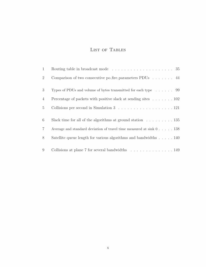
List of Tables
1 Routing table in broadcast mode . . . . . . . . . . . . . . . . . . . . 35
2 Comparison of two consecutive po fire parameters PDUs . . . . . . . 44
3 Types of PDUs and volume of bytes transmitted for each type . . . . . . 99
4 Percentage of packets with positive slack at sending sites . . . . . . . 102
5 Collisions per second in Simulation 3 . . . . . . . . . . . . . . . . . . 121
6 Slack time for all of the algorithms at ground station . . . . . . . . . 135
7 Average and standard deviation of travel time measured at sink 0 . . . . . 138
8 Satellite queue length for various algorithms and bandwidths . . . . . 140
9 Collisions at plane 7 for several bandwidths . . . . . . . . . . . . . . 149
x

List of Figures
1 The Flying network . . . . . . . . . . . . . . . . . . . . . . . . . . . . 26
2 Communication architecture model . . . . . . . . . . . . . . . . . . . 27
3 OMNeT screenshot of the whole network . . . . . . . . . . . . . . . . 30
4 Source file generator.ned . . . . . . . . . . . . . . . . . . . . . . . . . 32
5 File simplebus.ned . . . . . . . . . . . . . . . . . . . . . . . . . . . . 33
6 File sink.ned . . . . . . . . . . . . . . . . . . . . . . . . . . . . . . . . 34
7 Router onboard a plane and its connections . . . . . . . . . . . . . . 34
8 File router.ned . . . . . . . . . . . . . . . . . . . . . . . . . . . . . . 36
9 File satellite.ned . . . . . . . . . . . . . . . . . . . . . . . . . . . . . . 37
10 OMNeT representation of a computer node and its components . . . 38
11 Ned code of a computer node . . . . . . . . . . . . . . . . . . . . . . 38
12 Airplane view showing 3 computer nodes, a bus and a router . . . . . 39
13 OMNeT view of the ground station and its components . . . . . . . . 40
14 Ned Code of Ground Station . . . . . . . . . . . . . . . . . . . . . . . 40
15 Instantiation of the network TheNet . . . . . . . . . . . . . . . . . . 41
16 Initialization File Omnetpp.ini . . . . . . . . . . . . . . . . . . . . . . 43
17 Decision tree of the algorithm used by generators . . . . . . . . . . . 61
18 Overview of the simulation process . . . . . . . . . . . . . . . . . . . . . 74
xi

19 Sample of the contents of files datan.txt . . . . . . . . . . . . . . . . 75
20 Complete PDU of type po variable . . . . . . . . . . . . . . . . . . 76
21 Short PDU of type acknowledge . . . . . . . . . . . . . . . . . . . . . 77
22 PDU Type Distribution Generated in Simulation 1 . . . . . . . . . . 83
23 Minimum Bandwidth Requirements . . . . . . . . . . . . . . . . . . . 83
24 Slack Time at Generator 0 . . . . . . . . . . . . . . . . . . . . . . . . . 84
25 Travel Time as Sensed by the Ground Station . . . . . . . . . . . . . . . 85
26 Messages in Router 0 (plane 0) . . . . . . . . . . . . . . . . . . . . . . . 86
27 Messages in the Satellite . . . . . . . . . . . . . . . . . . . . . . . . . . 87
28 PDU Type Distribution Generated in Simulation 2 . . . . . . . . . . 89
29 Minimum Bandwidth Requirements . . . . . . . . . . . . . . . . . . . 90
30 Slack time to send next message at plane 0 and ground station (64 Kbps) . 90
31 Slack time to send next message by plane 0 (64 Kbps) . . . . . . . . . . . 91
32 Slack time to send next message by plane 0 and ground station (400 Kbps) 92
33 Travel times at plane 0 and ground station (64 Kbps) . . . . . . . . . . . 92
34 Travel times at plane 7 (64 Kbps) . . . . . . . . . . . . . . . . . . . . . 93
35 Travel times at plane 7 zoomed in (400 Kbps) . . . . . . . . . . . . . . . 94
36 Comparison of queue lengths of plane 0 and satellite (64 Kbps) . . . . . . 95
37 Comparison of queue lengths of plane 0 and satellite (400 Kbps) . . . . . 95
38 Collisions per second detected at plane 1 (64 Kbps) . . . . . . . . . . . . 96
39 Collision Accumulation over time at plane 7 (64 Kbps) . . . . . . . . . . 97
40 Distribution of PDUs in the simulation of MR1 vignette . . . . . . . 100
41 Minimum Bandwidth Requirements in Simulation 3 . . . . . . . . . . 101
xii
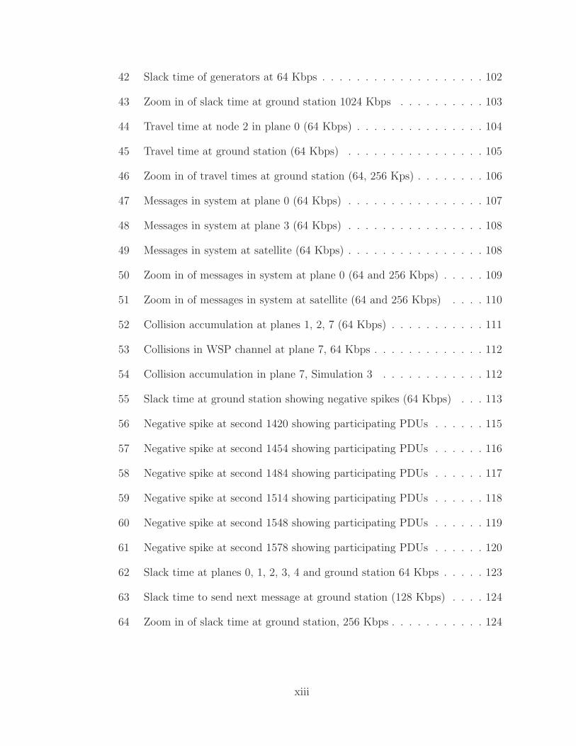
42 Slack time of generators at 64 Kbps . . . . . . . . . . . . . . . . . . . 102
43 Zoom in of slack time at ground station 1024 Kbps . . . . . . . . . . 103
44 Travel time at node 2 in plane 0 (64 Kbps) . . . . . . . . . . . . . . . 104
45 Travel time at ground station (64 Kbps) . . . . . . . . . . . . . . . . 105
46 Zoom in of travel times at ground station (64, 256 Kps) . . . . . . . . 106
47 Messages in system at plane 0 (64 Kbps) . . . . . . . . . . . . . . . . 107
48 Messages in system at plane 3 (64 Kbps) . . . . . . . . . . . . . . . . 108
49 Messages in system at satellite (64 Kbps) . . . . . . . . . . . . . . . . 108
50 Zoom in of messages in system at plane 0 (64 and 256 Kbps) . . . . . 109
51 Zoom in of messages in system at satellite (64 and 256 Kbps) . . . . 110
52 Collision accumulation at planes 1, 2, 7 (64 Kbps) . . . . . . . . . . . 111
53 Collisions in WSP channel at plane 7, 64 Kbps . . . . . . . . . . . . . 112
54 Collision accumulation in plane 7, Simulation 3 . . . . . . . . . . . . 112
55 Slack time at ground station showing negative spikes (64 Kbps) . . . 113
56 Negative spike at second 1420 showing participating PDUs . . . . . . 115
57 Negative spike at second 1454 showing participating PDUs . . . . . . 116
58 Negative spike at second 1484 showing participating PDUs . . . . . . 117
59 Negative spike at second 1514 showing participating PDUs . . . . . . 118
60 Negative spike at second 1548 showing participating PDUs . . . . . . 119
61 Negative spike at second 1578 showing participating PDUs . . . . . . 120
62 Slack time at planes 0, 1, 2, 3, 4 and ground station 64 Kbps . . . . . 123
63 Slack time to send next message at ground station (128 Kbps) . . . . 124
64 Zoom in of slack time at ground station, 256 Kbps . . . . . . . . . . . 124
xiii
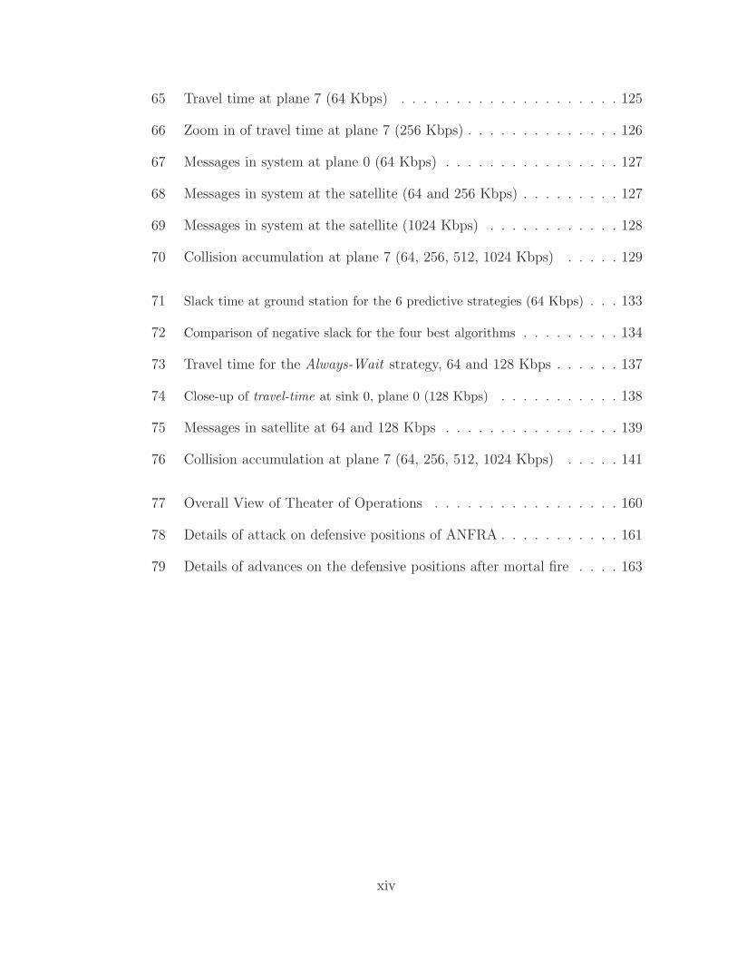
65 Travel time at plane 7 (64 Kbps) . . . . . . . . . . . . . . . . . . . . 125
66 Zoom in of travel time at plane 7 (256 Kbps) . . . . . . . . . . . . . . 126
67 Messages in system at plane 0 (64 Kbps) . . . . . . . . . . . . . . . . 127
68 Messages in system at the satellite (64 and 256 Kbps) . . . . . . . . . 127
69 Messages in system at the satellite (1024 Kbps) . . . . . . . . . . . . 128
70 Collision accumulation at plane 7 (64, 256, 512, 1024 Kbps) . . . . . 129
71 Slack time at ground station for the 6 predictive strategies (64 Kbps) . . . 133
72 Comparison of negative slack for the four best algorithms . . . . . . . . . 134
73 Travel time for the Always-Wait strategy, 64 and 128 Kbps . . . . . . 137
74 Close-up of travel-time at sink 0, plane 0 (128 Kbps) . . . . . . . . . . . 138
75 Messages in satellite at 64 and 128 Kbps . . . . . . . . . . . . . . . . 139
76 Collision accumulation at plane 7 (64, 256, 512, 1024 Kbps) . . . . . 141
77 Overall View of Theater of Operations . . . . . . . . . . . . . . . . . 160
78 Details of attack on defensive positions of ANFRA . . . . . . . . . . . 161
79 Details of advances on the defensive positions after mortal fire . . . . 163
xiv
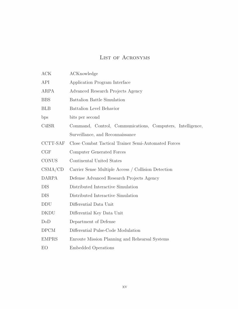
List of Acronyms
ACK ACKnowledge
API Application Program Interface
ARPA Advanced Research Projects Agency
BBS Battalion Battle Simulation
BLB Battalion Level Behavior
bps bits per second
C4ISR Command, Control, Communications, Computers, Intelligence,
Surveillance, and Reconnaissance
CCTT-SAF Close Combat Tactical Trainer Semi-Automated Forces
CGF Computer Generated Forces
CONUS Continental United States
CSMA/CD Carrier Sense Multiple Access / Collision Detection
DARPA Defense Advanced Research Projects Agency
DIS Distributed Interactive Simulation
DIS Distributed Interactive Simulation
DDU Differential Data Unit
DKDU Differential Key Data Unit
DoD Department of Defense
DPCM Differential Pulse-Code Modulation
EMPRS Enroute Mission Planning and Rehearsal Systems
EO Embedded Operations
xv
ES Embedded Simulation
ET Embedded Training
ESPDU Entity State Protocol Data Unit
FCS Future Combat System
INVEST Inter-Vehicle Embedded Simulation Technology
HITL Human-in-the-loop
HLA High Level Architecture
HoL Head of Line
JEMPRS Joint Enroute Mission Planning and Rehearsal System
JEMPRS-NT Joint Enroute Mission Planning and Rehearsal System Near-Term
Kbps Kilo bits per second
LAN Local Area Network
LBRM Log-Based Receiver-reliable Multicast
LZ Lempel-Ziv algorithm
MAC Medium Access Control
Mbps Mega bits per second
ModSAF Modular Semi-Automated Forces
NED Network topology Description language
NN Neural Network
OFET Objective Force Embedded Training
OMNeT++ Objective Modular Network Testbed in C++
OneSAF One Semi-Automated Forces
OPFOR Opposing Forces
OTB OneSAF Testbed Baseline
O&O Operations and Organizations
PDU Protocol Data Unit
PEO-STRI (U.S. Army) Program Executive Office for Simulation, Training, &
Instrumentation
PICA Protocol Independent Compression Algorithm
xvi
QES Quiescent Entity Service
QoS Quality of Service
RPC Remote Procedure Call
SAF Semi-Automated Forces
SIMNET SIMulation NETwork
SMS Switch-Memory-Switch
STOW-E AG Synthetic Theater of War–Europe Application Gateway
STRICOM US Army Simulation, Training and Instrumentation Command
TCP/IP Transmission Control Protocol / Internet Protocol
TDM Time Division Multiplexing
UA Unit of Action
UDP User Datagram Protocol
WAN Wide Area Network
WGS Wireless Ground station to Satellite link
WPP Wireless Plane to Plane link
WSP Wireless Satellite to Plane link
xvii
CHAPTER 1
INTRODUCTION
1.1 Overview
Computer modeling and simulation are commonly used in areas such as analysis
and prediction of behavior of complex systems, training, education, games, etc., and
has been applied to systems in all scientific disciplines such as Physics, Chemistry,
Engineering, Psychology, Sociology, Meteorology, etc.
The U. S. Department of Defense (DoD) defines a model as a physical,
mathematical, or otherwise logical representation of a system, entity, phenomenon,
or process, and a simulation as a method for implementing a model over time [Def94].
The DoD also classifies computer simulations in three broad categories called
live, virtual, and constructive simulation [US95b]. However, DoD recognizes that
the categorization of simulation into live, virtual, and constructive is problematic,
because there is no clear division between these categories. The degree of human
participation in the simulation is infinitely variable, as is the degree of equipment
realism. This categorization of simulations also suffers by excluding a category for
simulated people working real equipment (e.g., smart vehicles) [US98].
According to [US95b] and [US98], each category is defined as follows:
a. Live Simulation A simulation involving real people operating real systems.
1
b. Virtual Simulation A simulation involving real people operating simulated
systems. Virtual simulations inject human-in-the-loop (HITL) in a central
role by exercising motor control skills (e.g., flying an airplane), decision skills
(e.g., committing fire control resources to action), or communication skills
(e.g., as members of a C4I team).
c. Constructive Model or Simulation Models and simulations that involve
simulated people operating simulated systems. Real people stimulate (make
inputs) to such simulations, but are not involved in determining the outcomes.
Embedded Simulation (ES) integrates simulation technology with real systems,
providing the soldier with a chance to rehearse a mission in the real vehicle,
interacting with the virtual world as if it were real, and enhancing training
locally and in remote locations. The virtual interaction includes mission rehearsal,
battlefield visualization, command coordination, and training.
Objective Force Embedded Training (OFET) methods offer several distinct
advantages for 21st century training environments. Benefits include the ability to
perform in-situ exercises on actual equipment, more direct provision of support
for the variety of equipment in the field, and a greater opportunity to develop
new training exercises using much shorter lead times than were previously
possible with stand-alone training systems [BAC97]. A fully operational OFET
platform also presents several technology challenges. In particular, management
of Command, Control, Communications, Computers, Intelligence, Surveillance, and
Reconnaissance (C4ISR) resources is required for successful integration of simulation
within the actual environment.
The general project proposal from which this dissertation is one of the research
branches can be found in [GDD02], and the final report for its phase 2 is in [VGD03].
2

1.1.1 Development of OneSAF Testbed Baseline
As pointed out by McDonald [McD88], McDonald and Rullo [MR90], and
McDonald and Bahr [MB98a], [MB98b], in the late 1980’s Embedded Training (ET)
started as an important initiative of the US Army for training army personnel.
Among some of the reasons for developing ET there were budget cuts, security
interests, need to train forces by practicing missions without physically disturbing
cultural and environmental issues, etc. Other initiatives developed included
Embedded Operations (EO) and Embedded Simulation (ES). The three initiatives
had areas in common that facilitated the migration among them. The Inter-Vehicle
Embedded Simulation Technology (INVEST) program was proposed by the US
Army Simulation, Training and Instrumentation Command (STRICOM) in order
to explore key technologies to apply ET and ES to future ground combat vehicles.
Computer Generated Forces (CGF) was a project sponsored by DOD in
the 1990’s. The idea behind CGF is that the trainees need opposing forces
against which to rehearse, although they can also use them as friendly forces
to fight along with [HGG00]. These forces are generated by one or more of
the participating sites in the synthetic battlefield. Under CGF the two major
efforts were Modular Semi-Automated Forces (ModSAF) and Close Combat Tactical
Trainer Semi-Automated Forces (CCTT-SAF). In 1998, STRICOM started to
develop a recommendation of the SAF system to be used as the baseline for
integrating ModSAF and CCTT-SAF into a OneSAF Testbed Baseline (OTB).
OTB was planned to be used for supporting research and development for the
next generation of architecture experiments, extending toward providing a Battalion
Battle Simulation (BBS) replacement capability through a Battalion Level Behavior
(BLB) Application Program Interface (API), and providing the training capacity of
3
CCTT-SAF. Detailed information about the historic development of OTB can be
found in [Cor98] and [MWH01].
1.2 Distributed Simulation Environments
As Roger Herdman explains in [Tec95], Distributed Interactive Simulation (DIS)
is the linking of several military simulators like tank and aircraft in locations that
can be geographically distributed throughout LANs and WANs in such a way that
the crew of a given simulator can interact with crews in the other simulators playing
the roles of friendly or opposing forces. The participants can cooperate with friendly
forces, and shoot and destroy enemy ones. Command structures are also simulated.
In this way, the participants get trained in a broad range of scenarios without risking
their lives and at a fraction of the cost of a real operation.
The objective of DIS is to develop standards that provide guidelines for
interoperability in military simulations. DIS is a protocol initially specified in
ANSI/IEEE Std 1278-1993 Standard for Information Technology, Protocols for
Distributed Interactive Simulation [IEE93]. The standard has been refined and
extended in [IEE95a], [IEE95b], [IEE96], and [IEE98]. The main contribution of
the DIS standards was the definition of the Protocol Data Unit (PDU).
Because DIS is a stateless system that does not utilize servers, reliable multicast
communication is used to transmit information like terrain and environmental
updates. A Log-Based Receiver-reliable Multicast (LBRM) communication was
proposed in [HSC95] as a means to provide efficient DIS communications in
high-performance simulation applications. This reliability is given by a logging
server that logs all transmitted packets from the source. If a packet is lost, the
corresponding receiver asks the logging server to retransmit it. Another important
4
fact of the logging server is that at the end of the simulation the logged PDUs are
available for subsequent analysis, which is the case of the OTB logger. One successful
DIS application (precursor of OTB) was ModSAF, that simulates the hierarchy of
military units and their associated behaviors, combat vehicles, and weapons systems
[COM96].
A drawback in DIS is its high network bandwidth requirements and the large
computational loads placed on host computers. To overcome the problem, an agent
based architecture together with smart networks was proposed in [SZB96]. Mobile
agents consist of program scripts that are sent over the network to a remote server.
They contain state information and the executable code to be run in the remote
server, using the Remote Programming (RP) Paradigm. Remote programming
is different form the traditional Remote Procedure Call (RPC) in the sense that
not only the parameters but also the corresponding procedure is sent over the
network. The mobile agent can start its execution in one server, and continue
in another one by saving and attaching its state to itself. According to [SZB96],
Entity State PDUs (ESPDU) account for up to 70% of the network traffic. They
are used to communicate any change of state from one entity to the others, once a
given threshold is achieved. Also, DIS indicates that entities must send a heartbeat
message at specified time intervals, usually every five seconds, broadcasting their
state, so that if a new entity joins the simulation, it can be informed about all the
other entities already present. Also, every simulator broadcasts a Simulator Present
PDU every 20 seconds as a heartbeat message required by the Persistent Object
(PO) protocol implemented in ModSAF and OTB [Kir95]. If an entity is moving,
ESPDUs are sent at a higher rate than if it is still, but even still entities have to
inform its position at a given rate. Mobile agents can lower the usage of ESPDUs by
maintaining the positions of the still entities, instead of constantly sending ESPDU
messages.
5
1.3 Need for Simulation Communication Optimizations
In an embedded simulation system, the participating entities of a mission can
be physically separated by long distances, possibly onboard mobile vehicles, and
communicated via wireless channels. All the vehicles share a common virtual
world that has to be constantly updated, which carries realtime constraints on the
bandwidth, latency and connectivity of the subjacent network. OTB, for instance,
communicates through the PDU messages under the DIS protocol. Every time an
event occurs in a participating entity, like acceleration, firing, detonation, etc., a
PDU is broadcasted, making all the other entities aware of that event. Even if
nothing special is happening, the entities generate an ESPDU every five seconds as
a heartbeat to inform that the entity is still up and running [SZB96, Sri96].
In distributed simulation exercises it has been found that 50% to 80% of
the network traffic is originated from updates transmitted to ensure that all
the simulators have consistent information about the entities participating in the
simulated battlefield [CD96]. In order for the participants of the simulation to
interact with the virtual world in a realistic way, they must see and communicate
with each other in real time. To accomplish this, each simulator maintains
dead-reckoning models of its own state and of the state of all other vehicles with
which it may interact, and so the network used for embedded training must be able
to transfer massive volumes of data [HGG01].
Scalability is not only desirable, but a requirement of current simulation
protocols like HLA [WJ98]. Bandwidth is a scare resource, and the larger the number
of participating sites, the more compromise the available bandwidth becomes.
Stone [SZB96] indicates that the greatest problem currently facing the progress
of distributed simulations is scalability, and that it is very difficult to scale up
6
beyond approximately 2000 entities due to the tremendous requirements for network
bandwidth.
Several attempts have been done to overcome the bandwidth problem. The
general idea relies on finding new methods or algorithms to reduce the network
traffic, either by applying some lossless compression algorithms, by eliminating
some redundant packets, by splitting some PDUs into static and dynamic data
and sending the static data once and the dynamic data more often (delta-PDUs),
by concatenating (bundling) some PDUs into a larger packet that is later split at the
destinations into individual PDUs (replication), by re-scheduling some PDUs from
high intensive traffic spikes to periods of lower traffic demands, by using multicasting
instead of broadcasting, by applying priorities to PDUs and using Head of Line
(HOL) algorithms at router queues, or by applying a mix of all these ideas.
In this dissertation some of the previous methods are investigated. Re-scheduling
of the PDUs attempts to alleviate the occurrence of spikes of negative slack time
when OTB timestamps PDUs at exactly the same time. The basic idea is that it is
possible to slightly modify those timestamps in such a way that the overall simulation
is not affected, while exploiting the time interval of positive slacks following the
negative ones. The re-scheduling effect is automatically achieved by bundling those
PDUs and sending a single packet at a slightly later time.
Bundling and replication deal with sequences of several consecutive PDUs
timestamped at the same time or almost the same time, for instance PDUs of type
po fire parameters, which are the main cause of the said negative spikes. Basically,
these PDUs are copies of an initial base PDU. Then, a new method that eliminates
all the duplications is proposed. Bundling occurs at the sending sites and replication
is performed at the receiving ones.
7
1.4 Outline of This Dissertation
The rest of the document is divided in the following way. In Chapter 2,
PREVIOUS WORK, a review of the State of the Art in bandwidth assessment
for Embedded Simulations is given. The section Bundling And Aggregation of
Network Packets deals with current techniques for bundling PDUs. The section
Data Compression mentions some common compression techniques belonging to
the loss and lossless sets. The section Data Transmission refers to the possibility
of PDU rescheduling as a means of diminishing high traffic demands during short
periods of time. The chapter ends with the section Comparison of Techniques that
compares and contrasts the investigated techniques for making the most of the
available bandwidth.
In Chapter 3, COMMUNICATION RESOURCES AND ARCHITECTURE, the
Flying LAN is presented and serves as a framework for the rest of the document.
OMNeT is introduced along with the key concepts of model design, simple and
compound modules, and instantiation of the network, applied to the simulation at
hands.
In Chapter 4, ACTIVE BUNDLING STRATEGIES, the concepts of offline and
online bundling are stated, and how they relate to the algorithms proposed in this
dissertation. The characteristics of embedded simulation traffic impacting bundling
are exposed, and a description of the proposed offline and online algorithms is shown.
In Chapter 5, EMBEDDED SIMULATION TRAFFIC ANALYSIS, four
experiments are described. The general format of the input data is explained, and
two examples of actual PDUs are given. Simulation results are graphically presented
for each one of the experiments. In each case, an independent analysis consisting
of bandwidth statistics calculated before running the simulation are shown as a
means of predicting and corroborating the simulation outcomes. The PDU traffic is
8
then analyzed considering the criteria of slack time, travel time, queue length and
collision analysis. Spike analysis resulting from many observed negative spikes in
the slack time of the senders is studied in one of the experiments. A sample of some
negative spikes is collected, and the corresponding PDUs are identified, resulting in
interesting observations about the constant appearance of po fire parameters PDUs.
These observations are the key points for the proposed algorithm called PDUAlloy.
In Chapter 6, TRAFFIC OPTIMIZATION USING PDUAlloy, a new bundling
algorithm is proposed, and its behavior is analyzed by running the simulator.
Comparisons against the non-bundling algorithm are given. The conclusions indicate
that PDUAlloy is a successful algorithm, much better than the non-bundling
counterpart.
In Chapter 7, CONCLUSIONS, the results of the experiments are summarized
and general conclusions about the simulation tool, the methodology employed, PDU
traffic and minimum bandwidth requirements, are drawn.
In Chapter 8, FUTURE WORK, the continuation of the project is proposed.
Several areas are proposed for further research, related to new bundling options,
better prediction tools for upcoming PDUs, and the application of these techniques
to other communication protocols.
1.5 Contributions of This Dissertation
A summary of the main contributions made by this dissertation follows.
1. The formalization of the independent (offline) analysis for PDU traffic based
on availability of logged PDUs aimed at the assessment of minimum bandwidth
requirements for the network. The independent analysis provides a first
9

approximation to the minimum bandwidth requirements, which is a lot cheaper
than performing the actual simulation, perhaps having to run it several times
under different parameter combinations. Applied to the studied vignette and
without using simulation, the independent analysis estimated the required
bandwidth on 200 Kbps, which was later confirmed by the simulation.
2. The formalization of selective PDU bundling, called PDUAlloy. This kind
of bundling gets more active when it is needed the most: during negative
spikes of the slack time, and produces new packets that preserve the
internal PDU format, reason why the resulting packets can be considered
a new type of PDU. Due to that characteristic, bundled PDUs are subject
to further bundling and/or compression by more traditional techniques.
For example, if A and B are PDUs such that A = (a1, a2, a3, a4),
B = (b1, b2, b3, b4), and a2 = b2, a4 = b4, then the bundle A&B is
represented as (a1, a2, a3, a4, ((b1, 1), (b3, 3))). A simpler example could
be: (10, 8, 12, 20, 9)&(10, 6, 12, 20, 3) = (10, 8, 12, 20, 9, ((6, 2), (3, 5)))
3. The proposal and study of different predictive algorithms for the next PDU,
three of them on-line: neural network, Always-Wait and Always-Send,
and three off-line: type, type-and-length and type-length-and-size. Applying
Always-Wait to the studied vignette and setting the wireless links to 64 Kbps,
a reduction in the magnitude of negative slack time from -75 to -9 seconds
for the worst spike was achieved, which represents a spike reduction of 88%.
Similarly, at 64 Kbps Always-Wait reduced the average satellite queue length
from 2963 to 327 messages for a 89% reduction.
10

CHAPTER 2
PREVIOUS WORK
Many different solutions aimed at decreasing the network traffic have been
studied in the literature: bundling, delta-PDUs, dead-reckoning, relevance filtering,
compression, multicasting, quiescent entities, and the use of unreliable transport
mechanisms. Some of the most common bundling-related mechanisms are explained
next.
2.1 Bundling And Aggregation of Network Packets
Several authors have contributed to the principle of bundling packets, not only
applied to the DIS protocol, but also in other fields. In 1988 Baum and McMillan
applied the concept to messages traversing an hypercube network. They investigated
a mechanism for reducing the communication cost by bundling together messages
sent along the same channel, and concluded that the additional overhead required to
bundle the messages at the sending processor and to unbundle them at intermediate
processors is not large [BM88].
Calvin and Van Hook have proposed very similar definitions of bundling. They
say that bundling combines PDUs into larger packets in order to reduce packet
rates. A packet is transmitted when either a timer expires or the packet reaches a
maximum size. As a consequence, bit rates are reduced since fewer packet headers
11
are transmitted, placing multiple DIS PDUs in one single packet for transport
[CST95, VCR96].
Frederiksen and Larsen introduce a new parameter to the bundling
discussion: the necessary gap that must exist to separate physical packets in a
communication channel. They say that if data to be sent becomes available a little
at a time at irregular intervals, the sending side must decide whether to send a given
piece of data immediately or to wait for the next data to become available, such
that they can be sent together as a bundle [FL02]. The decision of sending is not
trivial because of physical properties of the networks requiring that after sending
each packet, a certain minimum amount of time (gap) must elapse before the next
packet may be sent. Thus, whereas waiting for more data will certainly delay the
transmission of the current data, sending immediately may delay the transmission
of the next data to become available even more [FL02].
In a recent article, Ceranowicz describes the Joint Experimental Federation
(JEF) and the Millennium Challenge 2002 (MC02), a simulation conducted in July
and August of 2002 by 13,500 personnel at locations across the United States. In the
article, he reports about the maximum limit of bytes that can be bundled. In one of
the experiments, up to to 4500 bytes were bundled in each IP packet and updates
were collected for up to one second. He concludes that the tradeoffs were that
bundling more data together increased latency and packet loss due to transmission
errors, while smaller packets increased the transmission of overhead data [CTH02].
In [BCL97] and [LCL99] consecutive PDUs are concatenated in a single packet
even if their types are different, and redundancy in the fields that make up a PDU
is not eliminated. Bassiouni explains that the benefit of PDU bundling comes from
the fact that network routers, bridges, gateways, and computer hosts have a limited
bound on the number of packets that they can process or transmit per second, and
12
bundling can effectively increase this bound. Bassiouni and Liang have the same
formalization of PDU bundling, which follows.
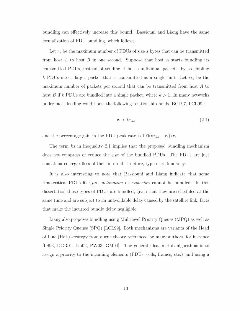
Let rs be the maximum number of PDUs of size s bytes that can be transmitted
from host A to host B in one second. Suppose that host A starts bundling its
transmitted PDUs, instead of sending them as individual packets, by assembling
k PDUs into a larger packet that is transmitted as a single unit. Let rks be the
maximum number of packets per second that can be transmitted from host A to
host B if k PDUs are bundled into a single packet, where k > 1. In many networks
under most loading conditions, the following relationship holds [BCL97, LCL99]:
rs < krks (2.1)
and the percentage gain in the PDU peak rate is 100(krks − rs)/rs
The term ks in inequality 2.1 implies that the proposed bundling mechanism
does not compress or reduce the size of the bundled PDUs. The PDUs are just
concatenated regardless of their internal structure, type or redundancy.
It is also interesting to note that Bassiouni and Liang indicate that some
time-critical PDUs like fire, detonation or explosion cannot be bundled. In this
dissertation those types of PDUs are bundled, given that they are scheduled at the
same time and are subject to an unavoidable delay caused by the satellite link, facts
that make the incurred bundle delay negligible.
Liang also proposes bundling using Multilevel Priority Queues (MPQ) as well as
Single Priority Queues (SPQ) [LCL99]. Both mechanisms are variants of the Head
of Line (HoL) strategy from queue theory referenced by many authors, for instance
[LS93, DGR01, Liu02, PW03, GM04]. The general idea in HoL algorithms is to
assign a priority to the incoming elements (PDUs, cells, frames, etc.) and using a
13

priority queue, serve the higher priority elements first, possibly defining timeouts
for the low priority ones so that starvation is prevented.
A delta-PDU encoding technique is mentioned in [US95a, Mac95] consisting of
PDUs that carry changes respect to a reference PDU initially given. The technique
exploits the fact that most information in DIS entity state PDUs is redundant
from one packet to the next. The delta-PDU encoding is accomplished by splitting
the DIS Entity State PDUs into static and dynamic data PDUs. The static data
becomes the reference PDU, while the dynamic one carries the changes. The idea
has also been studied for the HTTP protocol using intermediate proxy servers as
cache memory [MDF97, MDF02, WAS96]. Wills [WMS01] describes several delta
encoding and bundling techniques generally applicable to Web pages under the
TCP/IP protocol suite, but none is specific to the DIS protocol.
A protocol called DIS-Lite developed by MaK Technologies [Tay95, Tay96b,
Tay96a, PW98] also splits the Entity State PDU into static and dynamic data
PDUs, so that the static information is sent once and the changes (dynamic PDUs)
are subsequently sent as separate PDUs. DIS-Lite offers several advanced features,
including packet bundling, latency compensation and enhanced dead-reckoning
algorithms tailored for air vehicles [PW98]. According to [Ful96], by eliminating
redundancy DIS-Lite can perform between 30% and 70% more efficiently than DIS.
DIS-Lite also includes several other improvements not related to the combination
of individual fields from a set of similar PDUs. These objectives complement
related predictive strategies developed for conserving simulation bandwidth [BD96,
HGG01].
The bundling principle is also applied to TDM (Time Division Multiplexed)
networks, where a number of lower order frames are multiplexed into one higher
order frame [Ber02].
14
2.2 Data Compression
Data compression has been long studied and many papers have been written
around it. One of the goals of this dissertation is to diminish the bandwidth
requirements of OTB simulations by compressing the PDUs transmitted over the
network. It has been observed that in many cases the next PDUs are almost identical
to previously transmitted ones. This observation leads to the conclusion that it is
possible to apply one or several compression techniques to achieve better bandwidth
utilization.
Generally speaking, compression algorithms can be classified in two broad
categories: loss and lossless algorithms. Loss compression corresponds to algorithms
that do not guarantee an exact recovery of the compressed data. In many
applications like sound and video this loss is acceptable because human senses do
not detect the faults in the uncompress data, or because the final quality of the
uncompressed data is acceptable.
Lossless compression involves algorithms that can recover the original data
without faults. Applications include the transmission of an executable binary file,
or the compression/uncompression of TCP/IP packets. In this research, the lossless
compression of PDUs is sought. A detailed treatment of loss and lossless compression
algorithms is found in Deorowicz’s PhD dissertation [Deo03].
Compression algorithms can also be classified by the method employed to
compress the data. Some methods are based on dictionaries, guess tables or a
mix of both [Hew95, TS02]. Methods based on dictionaries create a dictionary of
strings commonly repeated in the data and corresponding keys much shorter than
the strings. Then, instead of the string, the key is transmitted. Obviously, each
communicating party needs to know the dictionary, which is transmitted in advance.
One of the most common lossless compression algorithms based on dictionaries is
15

the Lempel-Ziv (LZ) algorithm [ZL77] Common compressors like gzip, winzip and
pkzip are based on the LZ algorithm.
Guess tables are based on the idea that certain bytes can be guessed from the
previous transmitted ones. Both, the sending and receiving sites maintain the
same guess table. If the transmitter can guess the next byte, then that byte is
not transmitted but entered into the table.
Some algorithms are based on the concept of entropy taken from the information
theory to produce high compression rates. They are related to Shannon’s
fundamental source coding theorem [Sha48] and an example of this kind of
algorithms is Huffman coding [Huf52]. In [FY94] a lossless algorithm to compress
volume data based on differential pulse-code modulation (DPCM) and Huffman
coding is presented.
Compression algorithms have been devised specifically to compress network
packets. Dorward [DQ00] presents such an algorithm based on a variant
of Lempel-Ziv’s compression, and Ishac and Degermark [Ish01, DNP99] deal
specifically with TCP/IP headers. If the data to be transmitted in the TCP/IP
packets is too small, the transmission overhead of the headers starts to be an
important factor of bandwidth waste. The header compression combined with
data concatenation of several small PDU packets is then an appealing technique.
According to Degermark, header compression can decrease the header overhead for
IPv6/TCP from 19.5 per cent to less than 1 per cent for packets of 512 bytes.
TCP/IP compression has been researched by companies like Dataline
(http://www.dataline.com/) that claims that by using its TCP/IP acceleration
technology Joint En-route Mission Planning and Rehearsal System - Near Term
(JEMPRS-NT) can deliver the functionality required by a traveling team of
12-15 users over a satellite link. Dataline affirms that by using its technology,
a 64 Kbps link can give the equivalent throughput of a virtual 256 Kbps
16
[Fro02]. As an interesting observation, the simulations run in Chapter 6 using the
proposed bundling algorithm PDUAlloy, produced results comparable to Dataline’s
affirmation, just by employing bundling. The usage of several compression strategies
could lead to even better results.
There are two general classes of compression techniques for removing PDU
redundancies: application dependent and application independent. Algorithms that
fall in the first group know and take advantage of characteristics of the simulation
application like encoding data based on bit strings typical of the application and
sending delta PDUs. In the second group, algorithms are more general, do not
know particularities of the application and work by examining and compressing the
bit strings by detecting bit patterns. According to Van Hook [VCN94], application
dependent techniques can achieve slightly more compression than the independent
counterparts, but are a lot more complex and require much more processing power.
In 1994, Advanced Research Projects Agency (ARPA)s simulation exercise
called Synthetic Theater of War–Europe Application Gateway (STOW-E AG)
was conducted to test a new communication architecture. The AG was installed
between each site LAN and the WAN to apply several algorithms and techniques
for managing traffic flowing to and from each site, like blocking unnecessary PDUs,
Protocol Independent Compression Algorithm (PICA), grid filtering, Quiescent
Entity Service (QES), rethresholding, bundling, load leveling. Calvin reports that
the application of all these techniques produced a reduction in network traffic by
more than an order of magnitude [CST95].
PICA was originally proposed as a compression algorithm by Van Hook in 1994
to compress SIMNET PDUs [VCM94], achieving up to 76% reduction in bit rate.
The SIMNET protocol and simulation was a precursor of DIS protocol developed
in the late 1980’s by the Defense Advanced Research Projects Agency (DARPA).
PICA compresses ESPDUs by transmitting a reference ESPDU that becomes
17
known to the communicating entities, and subsequently sending delta-PDUs, also
called Differential Data Unit (DDU), containing those bytes which differ from the
reference ESPDU. Eventually, a new reference PDU, called Differential Key Data
Unit (DKDU), is transmitted because at that time the compression being achieved
by PICA falls below a threshold, due to increasingly larger bit pattern differences
[DCV94, VCN94, Fuj95]. PICA has been reported to yield fourfold compression
of entity state PDUs, although Fire, Detonation, and Collision PDUs are not
compressed before bundling, due to their relatively few number and small size
[VCN94]. However, in this dissertation, po fire PDUs are successfully compressed
because of the conditions (similar timestamps, long satellite link delays) specified
for the vignette.
2.3 Data Transmission
One of the goals in this dissertation consists of rescheduling some of the PDU
packets in order to better utilize the bandwidth by transferring PDUs from periods
of high activity to periods of low activity. As stated in the introduction, one of the
main causes of negative slack spikes is the scheduling of several PDUs at the same
time, which causes a bottleneck in the transmitting sites.
Packet rescheduling is an old technique, initially developed for the Ethernet
CSMA/CD protocol 802.3 [IEE85] to manage collisions during the contention period.
The exponential backoff algorithm is commonly used to reschedule the collided
packets, although Molle considers that the stability of the algorithm is somewhat
open to debate [Mol94]. If PDUs are timestamped at the same time, they can be
considered as a kind of collision that needs to be solved.
18
The scheduling of packet networks at the router level has been recently studied
in [APR03] where a randomized parallel scheduling algorithm for scheduling packets
in routers based on the Switch-Memory-Switch (SMS) architecture is developed.
Multicast routing algorithms and protocols with emphasis on QoS is addressed
in [WH00]. The network is represented as a weighted digraph with one or more
parameters associated to the links. Each parameter represents a characteristic
of the link, like transmission and propagation delay, bandwidth, etc. The nodes
also contain parameters that describe their stauts, like buffer space available,
queue length, etc. The multicast routing problem consists of finding minimum
spanning trees for a given objective function subject to QoS constraints. The
problem is classified into several categories depending on the objective functions
to be minimized and the QoS constraints. Examples of those categories
are: link constrained problems, tree constrained problems, link and tree constrained
problems, tree optimization problem, etc.
Packet transmission using priorities have been largely studied. The Head of Line
algorithms and priority queues are examples that make use of packet priorities. A
method that exploits a priority scheme to guarantee static preplanned message slots
for hard real-time communication is found in [KLJ00]. The mechanism is embedded
in the MAC layer. The method considers that there are highly time-critical messages
that require bounded transmission times. Applied to the present simulation, these
time-critical messages could be the po fire parameters PDUs involved in the negative
slack spikes.
Priorities are also used in real-time applications when the traffic is shared
with non real-time ones. A recent PhD dissertation by Pope addresses the issue
of bounding packet delay based on various queuing disciplines under real-time
constraints [Pop02].
19

2.4 Comparison of Bundling Techniques
The following list summarizes the most common bundling-related strategies used
to conserve bandwidth over WAN networks.
1. Plain concatenation of PDUs
• Consecutive PDUs are concatenated so that the total length of the bundle
is equal to the sum of the components.
• PDU types and timestamps are not decision variables
• Usually applied to ESPFUs, not fire and detonation ones.
• Each PDU conserves its own PDU header.
• Advantages: Savings in packet headers and ACK replies at the transport
layer, and separator gaps at the physical layer, by using a single header,
ACK and gap instead of many ones. Fewer collisions are produced
by having to acquire the channel fewer number of times, assuming a
CSMA/CD link.
• Disadvantages: Concatenation should be limited to the maximum size of
a network packet, to keep the previous advantages. Redundance is not
eliminated, and so fewer packets can be bundled in the same block.
2. IP header compression
• Consecutive IP headers having high similarity are compressed by a
lossless algorithm.
• Applicable to TCP/IP packets, not to PDUs.
• More useful if data segments are small in the packet.
20

• Advantages: By shortening the headers, less data is transmitted. Good
for short packets.
• Disadvantages: Low compression ratio for PDUs, given that they are not
compressed and in general are long. Redundancy is not eliminated.
3. Delta-PDUs
• A reference PDU is transmitted first, followed by packets carrying the
differences only.
• Destinations must keep the reference PDU in order to extract the original
PDUs from the deltas. This makes the PDUs dependent of the reference.
• After a threshold, a new reference PDU is transmitted
• Advantages: all the advantages of plain concatenation are applicable here,
plus high compression ratio.
• Disadvantages: delta PDUs are dependent on the reference PDU. If the
reference PDU gets lost or out of sequence (assuming unreliable UDP
transport), the deltas become useless and all the sequence have to be
retransmitted.
4. DIS-Lite
• Implements delta-PDUs and many other optimizations not related to
bundling.
• Terminology calls the reference and delta PDUs static and dynamic,
respectively.
• Tailored for air vehicle simulations, has been applied to video games
played on the internet.
21

• Advantages: all the advantages of delta-PDUs are valid here, as this
technique is a refinement of delta-PDUs. Involves several other
compression and bandwidth-saving techniques.
• Disadvantages: Has been applied to compression of ESPDUs only. Does
not examine and take advantage of the type, timestamp and internal
structure of PDUs. Mainly targeted at simulations of aircraft vehicles.
22
CHAPTER 3
COMMUNICATION RESOURCES AND
ARCHITECTURE
3.1 Simulation Vignette
A simulation environment aimed at assessing One Semi-Automated Force
(OneSAF) communications bandwidth during mission rehearsal of Future Combat
System (FCS) vignettes was developed at the Electrical and Computer Engineering
Department of the University of Central Florida, sponsored by the U.S. Army
Program Executive Office for Simulation, Training, & Instrumentation (PEO STRI),
formerly STRICOM.
Activities were undertaken to understand FCS mission rehearsal operations and
define a vignette to generate the simulation traffic to be modeled. The Operational
and Organizational (O&O) document [For02] entitled US Army Objective Force
Operational and Organizational Plan for Maneuver Unit of Action, TRADOC
525-3-90 /O&O, 22 July 2002 was obtained and reviewed for adaptation to our
vignette.
Several different FCS vignettes were prepared and simulated on a Local Area
Network (LAN) using the OneSAF Testbed Baseline (OTB) software, a military
simulation application that implements a Joint En-route Mission Planning and
Rehearsal System (JEMPRS) in an FCS environment. In [VDG04a, VDG04b],
23
the author describes an initial implementation of the OMNeT simulator used, and
corresponding results obtained when the vignette logs were run.
Traffic logs were created from the participating sites. OTB communications are
based on the Distributed Interactive Simulation (DIS) protocol defined in the IEEE
Standards 1278.1 [IEE95a], 1278.2 [IEE95b], 1278.3 [IEE96] and 1278.1a [IEE98].
The fundamental communication packets under DIS are the Protocol Data Units
(PDUs), which were logged including relevant PDU information used for alternative
parameter variations of the model. The information logged included the type,
length, and time-stamp of each PDU.
In particular, the MR1 vignette illustrating a mission rehearsal operation while
en-route to deployment and reproduced in Appendix A, was used to generate the
PDU traffic logs. This vignette was partly based on and extends TRADOC PAM
525-3-90 Operations & Organizations (O&O) document, “Annex F - Unit of Action
Vignettes [For02].” In the section called Statement Of Required Capabilities For
Future Combat Systems the TRADOC PAM document indicates that the Unit of
Action (UA) must be able to integrate into Enroute Mission Planning and Rehearsal
Systems (EMPRS) during alert, deployment and employment. FCS and Unit of
Action C2 systems must access enroute mission planning, and support mission
rehearsal, battle command, and ability to integrate into gaining C2 architectures
during movement by air, land and sea. The document contains three vignettes
including Entry Operations, Combined Arms Operations for Urban Warfare to
Secure Portion of Major Urban Area, and Mounted Formation Conducts Pursuit
and Exploration.
The duration of the MR1 vignette is approximately 25 minutes of simulation
time. It involves Entry Operations and Maneuver to Attack of a battalion-sized
unit tasked with pursuing an enemy delaying force immediately upon landing. The
lead elements (Alpha company) detect a fortified position between the main elements
24
and the target enemy force. Four RAH-66 Comanche helicopters are deployed and
follow closely. Next, the East friendly forces, begin to advance on the enemy position,
however, they must traverse minefields during their pursuit. The enemy force flees
southward from the North and East force. The South force engages the enemy, and
is assisted by the North and East forces.
The general scenario is that a Battalion Task Force equivalent has been rapidly
deployed. There are 8 aircraft, C-17 equivalent, in formation, each one carrying
up to three ground vehicles. Inside each aircraft, the vehicles are connected to
each other, and also to the aircraft communication resources, via a hardwired
Ethernet-type network. Each ground vehicle contains a computer station running
the MR1 vignette on OTB. The aircraft are in communication with each other
via satellite that also provides a link to a Continental United States (CONUS)
ground station. This ground station provides core exercise support including
Semi-Automated Forces (SAF). Additional links are utilized directly between the
aircraft to reduce demands on the satellite feed. This is based on SECOMP-1 /
JEMPRS Near-Term (JEMPRS-NT) architecture as of January 2003.
Figure 1 shows the model of the flying network used for rehearsal and training
on the MR1 vignette. The number of airplanes and simulation stations onboard
is variable in the model. The three simulation stations onboard each airplane are
connected at 100 Mbps. Connections from plane to plane are achieved via routers
and wireless links. Possible values for the wireless bandwidths range from 64 Kbps
to 1024 Kbps. Because the aircraft are flying in formation, the network is not
considered an ad hoc network.
The main stages in the development of the model included:
1. Design, obtain approval, and using OTB construct a vignette illustrating
mission rehearsal enroute to deployment.
25
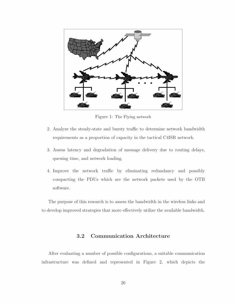
Figure 1: The Flying network
2. Analyze the steady-state and bursty traffic to determine network bandwidth
requirements as a proportion of capacity in the tactical C4ISR network.
3. Assess latency and degradation of message delivery due to routing delays,
queuing time, and network loading.
4. Improve the network traffic by eliminating redundancy and possibly
compacting the PDUs which are the network packets used by the OTB
software.
The purpose of this research is to assess the bandwidth in the wireless links and
to develop improved strategies that more effectively utilize the available bandwidth.
3.2 Communication Architecture
After evaluating a number of possible configurations, a suitable communication
infrastructure was defined and represented in Figure 2, which depicts the
26

communication architecture model used in most of the experiments performed. The
simulated model consists of eight airplanes flying in formation towards deployment.
Each aircraft carries three ground vehicles, and each vehicle contains a workstation
running OTB. Due to the proximity of the aircraft and the fact that they are flying
in a steady formation, all the planes and workstations conform a flying LAN.
Figure 2: Communication architecture model. Sites flagged T are transmitters, theothers are receivers.
Planes are numbered 0 to 7, and stations local to each plane are numbered 0 to
2, as well as 0 to 23 for the global network. The CONUS ground station is numbered
24. Routers are numbered the same as the plane they are onboard. According to
the data logged form the vignette, some stations are transmitters while others are
just receivers. The stations flagged “T” represent packet transmitters; the others
are the receivers. But according to the DIS protocol, the transmitters broadcast
their packets, and so transmitters are receivers, too.
The number of airplanes, computers onboard and channel bandwidth is not
a tight restriction in the model. The three computers onboard the airplanes are
27
connected via Ethernet cable or similar. Connections from plane to plane are done
via routers and wireless links. The bandwidth of the wireless connections is initially
set to 64 Kbps, and different runs of the simulator using speeds of 128, 200, 256,
512, and 1024 Kbps are carried out. The Ethernet LAN is maintained at 100 Mbps
in all cases, due to the fact that this technology is very common nowadays, and
the LAN bandwidth is at least two orders of magnitude greater than the wireless
bandwidth. A ground station is connected to the flying network through a satellite
link. All the computers in the network use the DIS protocol to broadcast messages,
as specified in [IEE95a].
An object of type bus models all the communication links. A bus contains input
and output connectors separated by known distances. Each bus is configured to
operate at a specific bandwidth and propagation delay. When a message enters
through one of the input connectors, the bus delivers it to each of the output
connectors at different times depending on the distance and propagation delay of
the medium. The bus was programmed so that signals propagate through it in
both directions. If (ICi, OCi) is a pair of input and output connectors located at
a distance di from one of the bus endpoints, p is the propagation delay in the bus
(nanoseconds/meter), b is the bus bandwidth (bps), and a message of length n
bits arrives into (IC i at time t, then when the message reaches any other output
connector OC j the following measures hold:
Distancetraveled = |di − dj| (3.1)
Propagationdelay = Distancetraveled ∗ p (3.2)
Transmissiontime = n/b (3.3)
StarttimeatOC j = t + Propagationdelay
= t + |d(i − dj| ∗ p (3.4)
EndtimeatOC j = start + transmissiontime
28
= t + |di − dj| ∗ p + n/b (3.5)
The start and end times at OC j are useful to determine collisions. If a message
has a time interval defined by start and end times overlapping the time interval
defined by the start and end times at OC j of any other message, then a collision
occurs.
Generalizing, the model can be described as a collection of computer nodes and
routers interconnected by different media at several bandwidths. The transmitters
broadcast packets at unspecified rates. In order to generate the packets, it is possible
to use a specific probability distribution over time. However, to obtain maximum
accuracy, a log of the actual packets generated by OTB, including the PDU type,
time-stamp, and packet length was used in place of a random distribution function,
providing more realism to the results.
3.3 Transmission and Receiving Devices
The OMNeT++ discrete event simulator was used as the main tool for the
model setup. OMNeT++ was designed by Andras Varga [Var03] at the University
of Budapest. The kernel was written in C++, and the user specifies additional
modules to program the behavior of the entities in the model. The model design
follows a bottom-up approach for modeling the communication architecture. Simple
modules are built first and compound modules are built on top of the simple ones.
Figure 3 gives a general view of the simple and compound modules of the simulator
connected together. It is an actual screenshot of the main OMNeT++ window. If
the simulator is run with the animation option activated, each one of the traveling
29
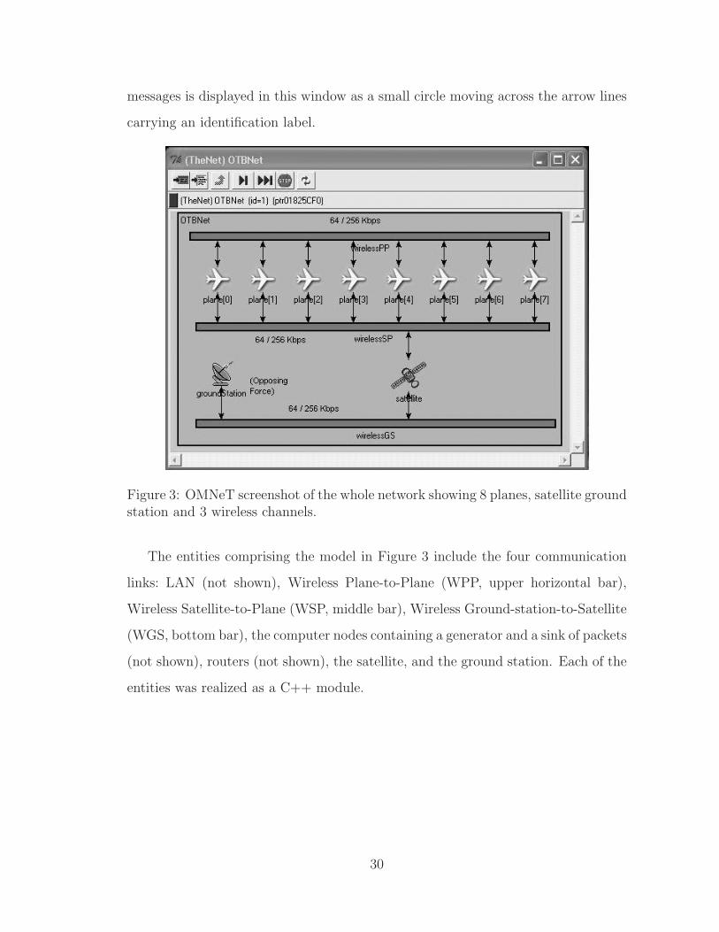
messages is displayed in this window as a small circle moving across the arrow lines
carrying an identification label.
Figure 3: OMNeT screenshot of the whole network showing 8 planes, satellite groundstation and 3 wireless channels.
The entities comprising the model in Figure 3 include the four communication
links: LAN (not shown), Wireless Plane-to-Plane (WPP, upper horizontal bar),
Wireless Satellite-to-Plane (WSP, middle bar), Wireless Ground-station-to-Satellite
(WGS, bottom bar), the computer nodes containing a generator and a sink of packets
(not shown), routers (not shown), the satellite, and the ground station. Each of the
entities was realized as a C++ module.
30
3.3.1 Simple Modules in OMNeT
These are modules that contain no other modules inside them. They are used
to describe the most basic elements of the simulator. Generators of messages,
sinks or consumers of messages, communication channels (wireless and Ethernet
buses), routers and the satellite correspond to simple modules. Each simple module
is defined by two files. The first is a .ned file that describes input parameters
to the module and the set of input and output gates or communication ports.
The second is a C++ source file that defines the behavior of the module, i.e. it
indicates how to process each message received through any of the input gates
and which messages to send through the output gates. The simulator in this
project includes the following .ned files of simple modules: generator.ned,
simplebus.ned, sink.ned, router.ned, and satellite.ned. Figures 4 to 9
show the corresponding ned source codes.
3.3.1.1 The Generators
A generator is the module that produces new messages, following the instructions
in the corresponding C++ file. The module reads in a sequence of PDUs from a
summary file containing the type, length and timestamp. When the simulation time
has reached the timestamp of a message, the generator outputs that packet to the
LAN link if it is onboard an airplane, or to the WGS link if it is in the ground
station.
After sending a packet, employing the transmission time corresponding to the
packet length and bus bandwidth, an inter-frame space (IFS) or time gap of 50
31
µseconds is added, in accordance with the specifications given in ANSI/IEEE
protocol 802.11 [IEE99].
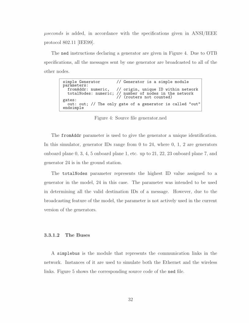
The ned instructions declaring a generator are given in Figure 4. Due to OTB
specifications, all the messages sent by one generator are broadcasted to all of the
other nodes.
simple Generator // Generator is a simple moduleparameters:fromAddr: numeric, // origin, unique ID within networktotalNodes: numeric; // number of nodes in the network
// (routers not counted)gates:out: out; // The only gate of a generator is called "out"
endsimple
Figure 4: Source file generator.ned
The fromAddr parameter is used to give the generator a unique identification.
In this simulator, generator IDs range from 0 to 24, where 0, 1, 2 are generators
onboard plane 0, 3, 4, 5 onboard plane 1, etc. up to 21, 22, 23 onboard plane 7, and
generator 24 is in the ground station.
The totalNodes parameter represents the highest ID value assigned to a
generator in the model, 24 in this case. The parameter was intended to be used
in determining all the valid destination IDs of a message. However, due to the
broadcasting feature of the model, the parameter is not actively used in the current
version of the generators.
3.3.1.2 The Buses
A simplebus is the module that represents the communication links in the
network. Instances of it are used to simulate both the Ethernet and the wireless
links. Figure 5 shows the corresponding source code of the ned file.
32
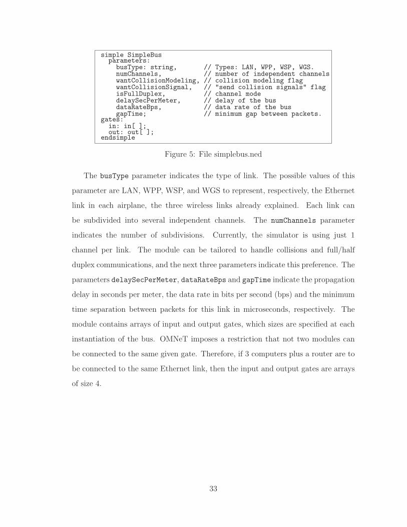
simple SimpleBusparameters:
busType: string, // Types: LAN, WPP, WSP, WGS.numChannels, // number of independent channelswantCollisionModeling, // collision modeling flagwantCollisionSignal, // "send collision signals" flagisFullDuplex, // channel modedelaySecPerMeter, // delay of the busdataRateBps, // data rate of the busgapTime; // minimum gap between packets.
gates:in: in[ ];out: out[ ];
endsimple
Figure 5: File simplebus.ned
The busType parameter indicates the type of link. The possible values of this
parameter are LAN, WPP, WSP, and WGS to represent, respectively, the Ethernet
link in each airplane, the three wireless links already explained. Each link can
be subdivided into several independent channels. The numChannels parameter
indicates the number of subdivisions. Currently, the simulator is using just 1
channel per link. The module can be tailored to handle collisions and full/half
duplex communications, and the next three parameters indicate this preference. The
parameters delaySecPerMeter, dataRateBps and gapTime indicate the propagation
delay in seconds per meter, the data rate in bits per second (bps) and the minimum
time separation between packets for this link in microseconds, respectively. The
module contains arrays of input and output gates, which sizes are specified at each
instantiation of the bus. OMNeT imposes a restriction that not two modules can
be connected to the same given gate. Therefore, if 3 computers plus a router are to
be connected to the same Ethernet link, then the input and output gates are arrays
of size 4.
33
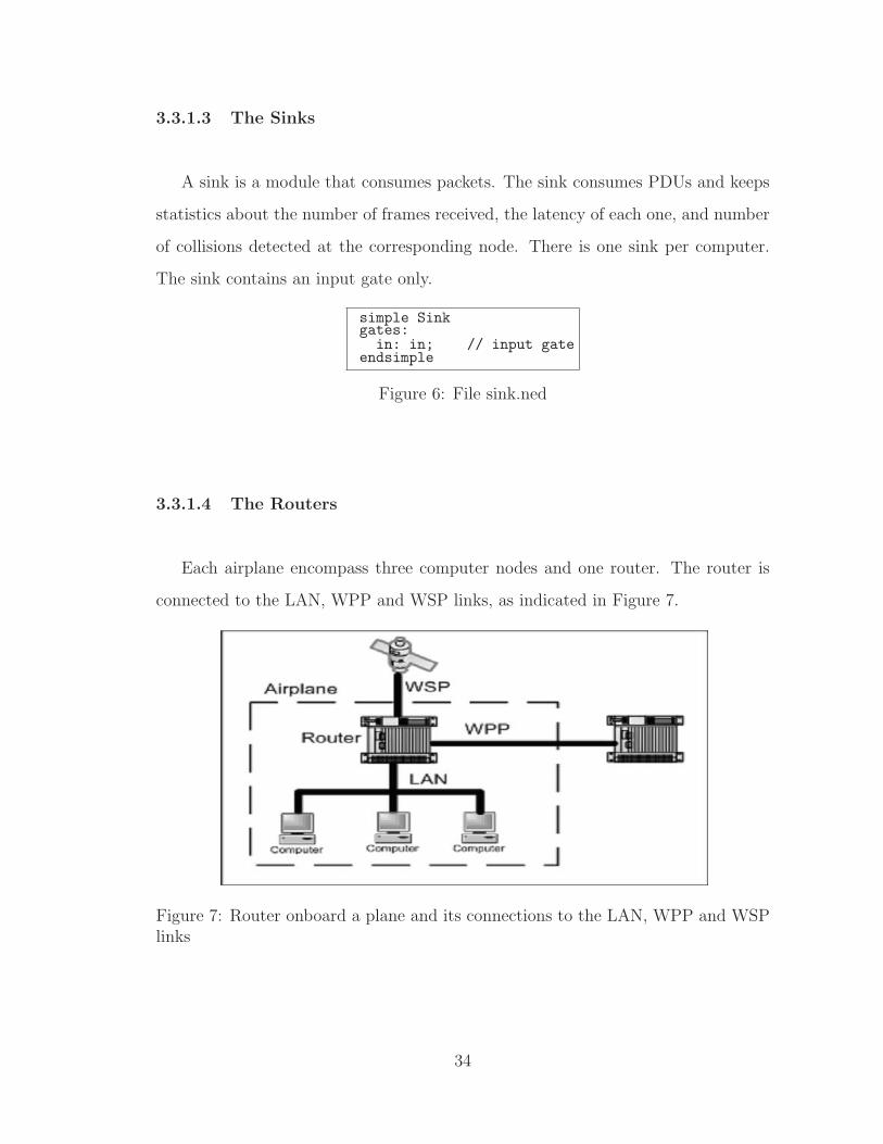
3.3.1.3 The Sinks
A sink is a module that consumes packets. The sink consumes PDUs and keeps
statistics about the number of frames received, the latency of each one, and number
of collisions detected at the corresponding node. There is one sink per computer.
The sink contains an input gate only.
simple Sinkgates:in: in; // input gate
endsimple
Figure 6: File sink.ned
3.3.1.4 The Routers
Each airplane encompass three computer nodes and one router. The router is
connected to the LAN, WPP and WSP links, as indicated in Figure 7.
Figure 7: Router onboard a plane and its connections to the LAN, WPP and WSPlinks
34
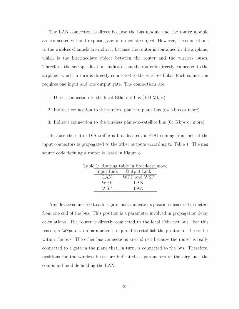
The LAN connection is direct because the bus module and the router module
are connected without requiring any intermediate object. However, the connections
to the wireless channels are indirect because the router is contained in the airplane,
which is the intermediate object between the router and the wireless buses.
Therefore, the ned specifications indicate that the router is directly connected to the
airplane, which in turn is directly connected to the wireless links. Each connection
requires one input and one output gate. The connections are:
1. Direct connection to the local Ethernet bus (100 Mbps)
2. Indirect connection to the wireless plane-to-plane bus (64 Kbps or more)
3. Indirect connection to the wireless plane-to-satellite bus (64 Kbps or more)
Because the entire DIS traffic is broadcasted, a PDU coming from one of the
input connectors is propagated to the other outputs according to Table 1. The ned
source code defining a router is listed in Figure 8.
Table 1: Routing table in broadcast modeInput Link Output Link
LAN WPP and WSPWPP LANWSP LAN
Any device connected to a bus gate must indicate its position measured in meters
from one end of the bus. This position is a parameter involved in propagation delay
calculations. The router is directly connected to the local Ethernet bus. For this
reason, a LANposition parameter is required to establish the position of the router
within the bus. The other bus connections are indirect because the router is really
connected to a gate in the plane that, in turn, is connected to the bus. Therefore,
positions for the wireless buses are indicated as parameters of the airplane, the
compound module holding the LAN.
35
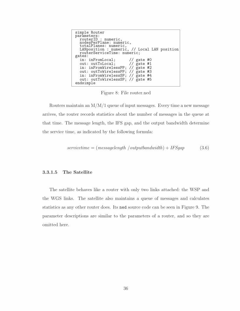
simple Routerparameters:
routerID : numeric,nodesPerPlane: numeric,totalPlanes: numeric,LANposition : numeric, // Local LAN positionrouterServiceTime: numeric;
gates:in: inFromLocal; // gate #0out: outToLocal; // gate #1in: inFromWirelessPP; // gate #2out: outToWirelessPP; // gate #3in: inFromWirelessSP; // gate #4out: outToWirelessSP; // gate #5
endsimple
Figure 8: File router.ned
Routers maintain an M/M/1 queue of input messages. Every time a new message
arrives, the router records statistics about the number of messages in the queue at
that time. The message length, the IFS gap, and the output bandwidth determine
the service time, as indicated by the following formula:
servicetime = (messagelength /outputbandwidth) + IFSgap (3.6)
3.3.1.5 The Satellite
The satellite behaves like a router with only two links attached: the WSP and
the WGS links. The satellite also maintains a queue of messages and calculates
statistics as any other router does. Its ned source code can be seen in Figure 9. The
parameter descriptions are similar to the parameters of a router, and so they are
omitted here.
36

simple Satelliteparameters:
satelliteID : numeric,satServiceTime : numeric,totalNodes : numeric,WGSposition : numeric, // Position at wirelessGSWSPposition : numeric; // Position at wirelessSP
gates:in: inBus1; // gate #0 (wirelessGS)out: outBus1; // gate #1 (wirelessGS)in: inBus2; // gate #2 (wirelessSP)out: outBus2; // gate #3 (wirelessSP)
endsimple
Figure 9: File satellite.ned
3.3.2 Compound Modules
Compound modules are modules that contain other modules inside. For example,
a computer onboard an airplane is a compound module because it contains a message
generator and a sink. A plane is also a compound module that contains a computer,
a router and an Ethernet bus. The largest compound module corresponds to the
whole network that contains the airplanes, the satellite, the ground station, and
the wireless buses linking these elements. Each one of these compound modules is
briefly discussed in the following paragraphs.
3.3.3 The Flying Computer Nodes
Each workstation in the model consists of a computer node that contains two
other submodules: the generator and the sink of PDUs. These computer nodes are
directly connected to the LAN link. Figure 10 shows the OMNeT++ representation
of a computer node, and Figure 11 lists its ned source code. The module Node
is composed of the simple modules gen (generator) and sink. The module also
contains an input (in) and an output (out) gate.
37
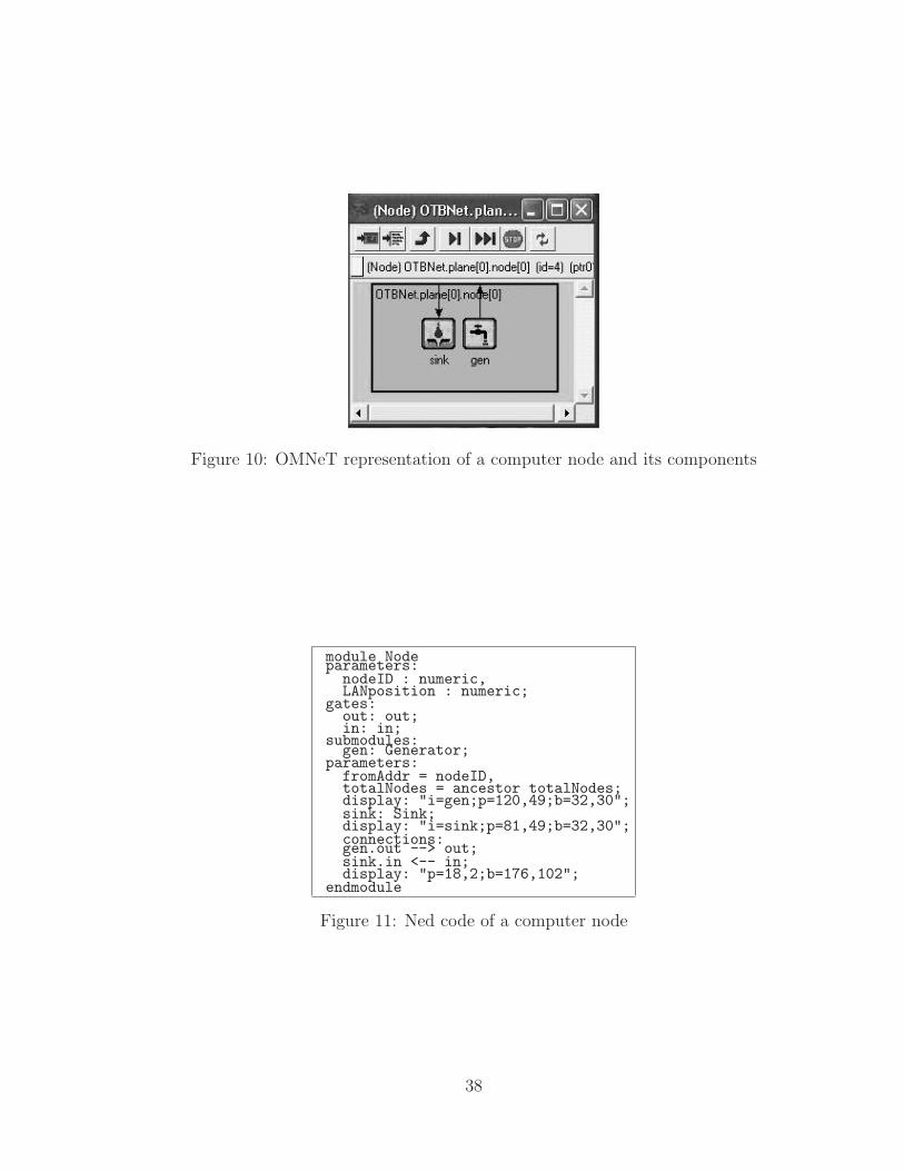
Figure 10: OMNeT representation of a computer node and its components
module Nodeparameters:nodeID : numeric,LANposition : numeric;
gates:out: out;in: in;
submodules:gen: Generator;
parameters:fromAddr = nodeID,totalNodes = ancestor totalNodes;display: "i=gen;p=120,49;b=32,30";sink: Sink;display: "i=sink;p=81,49;b=32,30";connections:gen.out --> out;sink.in <-- in;display: "p=18,2;b=176,102";
endmodule
Figure 11: Ned code of a computer node
38
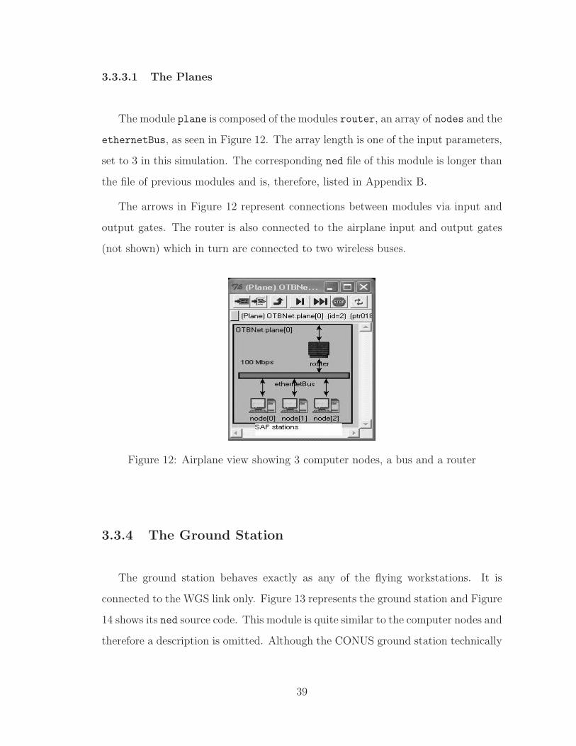
3.3.3.1 The Planes
The module plane is composed of the modules router, an array of nodes and the
ethernetBus, as seen in Figure 12. The array length is one of the input parameters,
set to 3 in this simulation. The corresponding ned file of this module is longer than
the file of previous modules and is, therefore, listed in Appendix B.
The arrows in Figure 12 represent connections between modules via input and
output gates. The router is also connected to the airplane input and output gates
(not shown) which in turn are connected to two wireless buses.
Figure 12: Airplane view showing 3 computer nodes, a bus and a router
3.3.4 The Ground Station
The ground station behaves exactly as any of the flying workstations. It is
connected to the WGS link only. Figure 13 represents the ground station and Figure
14 shows its ned source code. This module is quite similar to the computer nodes and
therefore a description is omitted. Although the CONUS ground station technically
39
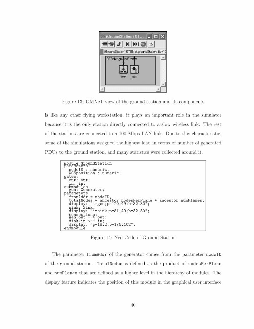
Figure 13: OMNeT view of the ground station and its components
is like any other flying workstation, it plays an important role in the simulator
because it is the only station directly connected to a slow wireless link. The rest
of the stations are connected to a 100 Mbps LAN link. Due to this characteristic,
some of the simulations assigned the highest load in terms of number of generated
PDUs to the ground station, and many statistics were collected around it.
module GroundStationparameters:nodeID : numeric,WGSposition : numeric;
gates:out: out;in: in;
submodules:gen: Generator;
parameters:fromAddr = nodeID,totalNodes = ancestor nodesPerPlane * ancestor numPlanes;display: "i=gen;p=120,49;b=32,30";sink: Sink;display: "i=sink;p=81,49;b=32,30";connections:gen.out --> out;sink.in <-- in;display: "p=18,2;b=176,102";
endmodule
Figure 14: Ned Code of Ground Station
The parameter fromAddr of the generator comes from the parameter nodeID
of the ground station. TotalNodes is defined as the product of nodesPerPlane
and numPlanes that are defined at a higher level in the hierarchy of modules. The
display feature indicates the position of this module in the graphical user interface
40

(GUI). Finally, the module establishes the connections between the gates from the
inner (simple) modules and the container module (the ground station).
3.3.5 Instantiation of the Network
The compound module TheNet contains the submodules wirelessPP,
wirelessSP, wirelessGS, groundStation, satellite, and plane as shown in
Figure 3. Due to its length, the source code of the ned language for this module is
found in Appendix B.
OMNeT++ uses the object programming approach. The modules as well as the
whole network are considered classes that must be instantiated. In this simulation
TheNet is the class name of the network that is instantiated as Network OTBNet.
It includes all of the model parameters that are read from the omnetpp.ini file.
Figure 15 shows this instantiation and the corresponding parameters.
network OTBNet : TheNetparameters:startTime = input, //First PDU timestamp in secondsnodesPerPlane = input,//Set to 3 in this simulationnumPlanes = input, //Set to 8 in this simulationLANgapTime = input, //Minimum gap between frames in LANLANbandwidth = input, //Set to 100 MbpsLANdelay = input, //nanosec/meter (70% light speed)WPPgapTime = input, //Minimum gap between frames in WPPWPPbandwidth = input, //Wireless bandwidth in WPPWPPdelay = input, //nanosec/meter (light speed)WSPgapTime = input, //Minimum gap between frames in WSPWSPbandwidth = input, //Wireless bandwidth in WSPWSPdelay = input, //nanosec/meter (light speed)WGSgapTime = input, //Minimum gap between frames in WGSWGSbandwidth = input, //Wireless bandwidth WGSWGSdelay = input, //nanosec/meter (light speed)satServiceTime = input, //Satellite service timerouterServiceTime = input; //Router service time
endnetwork
Figure 15: Instantiation of the network TheNet
41
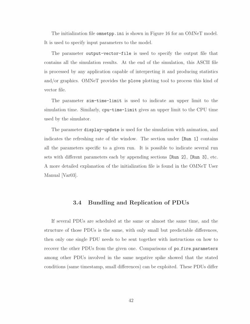
The initialization file omnetpp.ini is shown in Figure 16 for an OMNeT model.
It is used to specify input parameters to the model.
The parameter output-vector-file is used to specify the output file that
contains all the simulation results. At the end of the simulation, this ASCII file
is processed by any application capable of interpreting it and producing statistics
and/or graphics. OMNeT provides the plove plotting tool to process this kind of
vector file.
The parameter sim-time-limit is used to indicate an upper limit to the
simulation time. Similarly, cpu-time-limit gives an upper limit to the CPU time
used by the simulator.
The parameter display-update is used for the simulation with animation, and
indicates the refreshing rate of the window. The section under [Run 1] contains
all the parameters specific to a given run. It is possible to indicate several run
sets with different parameters each by appending sections [Run 2], [Run 3], etc.
A more detailed explanation of the initialization file is found in the OMNeT User
Manual [Var03].
3.4 Bundling and Replication of PDUs
If several PDUs are scheduled at the same or almost the same time, and the
structure of those PDUs is the same, with only small but predictable differences,
then only one single PDU needs to be sent together with instructions on how to
recover the other PDUs from the given one. Comparisons of po fire parameters
among other PDUs involved in the same negative spike showed that the stated
conditions (same timestamp, small differences) can be exploited. These PDUs differ
42
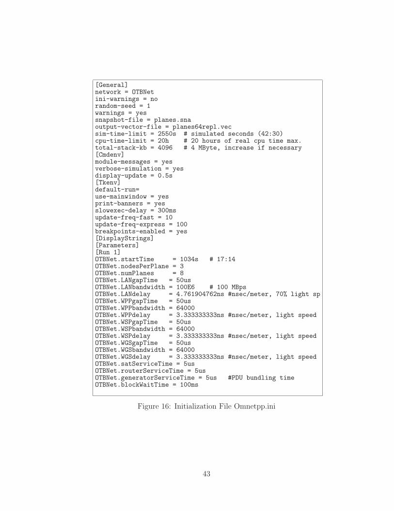
[General]network = OTBNetini-warnings = norandom-seed = 1warnings = yessnapshot-file = planes.snaoutput-vector-file = planes64repl.vecsim-time-limit = 2550s # simulated seconds (42:30)cpu-time-limit = 20h # 20 hours of real cpu time max.total-stack-kb = 4096 # 4 MByte, increase if necessary[Cmdenv]module-messages = yesverbose-simulation = yesdisplay-update = 0.5s[Tkenv]default-run=use-mainwindow = yesprint-banners = yesslowexec-delay = 300msupdate-freq-fast = 10update-freq-express = 100breakpoints-enabled = yes[DisplayStrings][Parameters][Run 1]OTBNet.startTime = 1034s # 17:14OTBNet.nodesPerPlane = 3OTBNet.numPlanes = 8OTBNet.LANgapTime = 50usOTBNet.LANbandwidth = 100E6 # 100 MBpsOTBNet.LANdelay = 4.761904762ns #nsec/meter, 70% light spOTBNet.WPPgapTime = 50usOTBNet.WPPbandwidth = 64000OTBNet.WPPdelay = 3.333333333ns #nsec/meter, light speedOTBNet.WSPgapTime = 50usOTBNet.WSPbandwidth = 64000OTBNet.WSPdelay = 3.333333333ns #nsec/meter, light speedOTBNet.WGSgapTime = 50usOTBNet.WGSbandwidth = 64000OTBNet.WGSdelay = 3.333333333ns #nsec/meter, light speedOTBNet.satServiceTime = 5usOTBNet.routerServiceTime = 5usOTBNet.generatorServiceTime = 5us #PDU bundling timeOTBNet.blockWaitTime = 100ms
Figure 16: Initialization File Omnetpp.ini
43
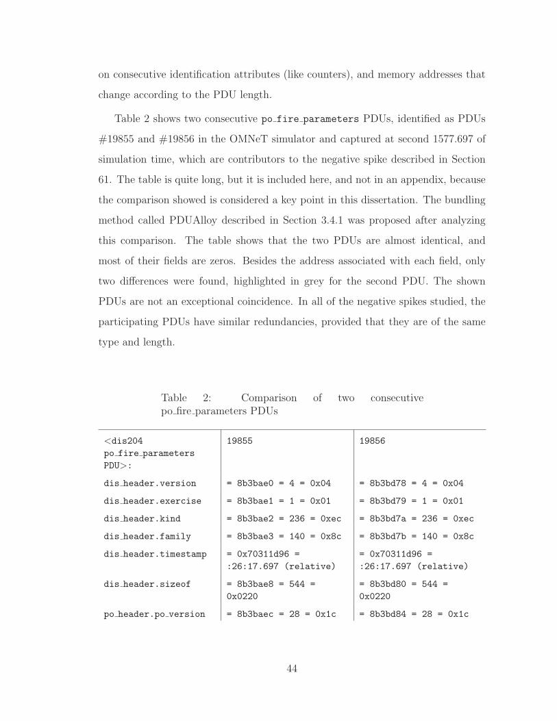
on consecutive identification attributes (like counters), and memory addresses that
change according to the PDU length.
Table 2 shows two consecutive po fire parameters PDUs, identified as PDUs
#19855 and #19856 in the OMNeT simulator and captured at second 1577.697 of
simulation time, which are contributors to the negative spike described in Section
61. The table is quite long, but it is included here, and not in an appendix, because
the comparison showed is considered a key point in this dissertation. The bundling
method called PDUAlloy described in Section 3.4.1 was proposed after analyzing
this comparison. The table shows that the two PDUs are almost identical, and
most of their fields are zeros. Besides the address associated with each field, only
two differences were found, highlighted in grey for the second PDU. The shown
PDUs are not an exceptional coincidence. In all of the negative spikes studied, the
participating PDUs have similar redundancies, provided that they are of the same
type and length.
Table 2: Comparison of two consecutivepo fire parameters PDUs
<dis204po fire parametersPDU>:
19855 19856
dis header.version = 8b3bae0 = 4 = 0x04 = 8b3bd78 = 4 = 0x04
dis header.exercise = 8b3bae1 = 1 = 0x01 = 8b3bd79 = 1 = 0x01
dis header.kind = 8b3bae2 = 236 = 0xec = 8b3bd7a = 236 = 0xec
dis header.family = 8b3bae3 = 140 = 0x8c = 8b3bd7b = 140 = 0x8c
dis header.timestamp = 0x70311d96 =:26:17.697 (relative)
= 0x70311d96 =:26:17.697 (relative)
dis header.sizeof = 8b3bae8 = 544 =0x0220
= 8b3bd80 = 544 =0x0220
po header.po version = 8b3baec = 28 = 0x1c = 8b3bd84 = 28 = 0x1c
44

po header.po kind = 8b3baed = 2 = 0x02 = 8b3bd85 = 2 = 0x02
po header.exerciseid
= 8b3baee = 1 = 0x01 = 8b3bd86 = 1 = 0x01
po header.databaseid
= 8b3baef = 1 = 0x01 = 8b3bd87 = 1 = 0x01
po header.length = 8b3baf0 = 528 =0x0210
= 8b3bd88 = 528 =0x0210
po header.pdu count = 8b3baf2 = 9215 =0x23ff
= 8b3bd8a =9216 = 0x2400
do header.databasesequence number
= 8b3baf4 = 0 =0x00000000
= 8b3bd8c = 0 =0x00000000
do header.objectid.simulator.site
= 8b3baf8 = 1532 =0x05fc
= 8b3bd90 = 1532 =0x05fc
do header.objectid.simulator.host
= 8b3bafa = 47451 =0xb95b
= 8b3bd92 = 47451 =0xb95b
do header.objectid.object
= 8b3bafc = 2898 =0x0b52
= 8b3bd94 = 2898 =0x0b52
do header.worldstate id.simulator.site
= 8b3bafe = 0 = 0x0000 = 8b3bd96 = 0 = 0x0000
do header.worldstate id.simulator.host
= 8b3bb00 = 0 = 0x0000 = 8b3bd98 = 0 = 0x0000
do header.worldstate id.object
= 8b3bb02 = 0 = 0x0000 = 8b3bd9a = 0 = 0x0000
do header.owner .site = 8b3bb04 = 1532 =0x05fc
= 8b3bd9c = 1532 =0x05fc
do header.owner .host = 8b3bb06 = 47451 =0xb95b
= 8b3bd9e = 47451 =0xb95b
do header.sequencenumber
= 8b3bb08 = 17 = 0x0011 = 8b3bda0 =18 = 0x0012
do header.class = 8b3bb0a = 19 = 0x13 = 8b3bda2 = 19 = 0x13
do header.missingfrom world state
= 8b3bb0b = 0 =0x00000000
= 8b3bda3 = 0 =0x00000000
reserved9 = 8b3bb0c = 0 =0x00000000
= 8b3bda4 = 0 =0x00000000
45
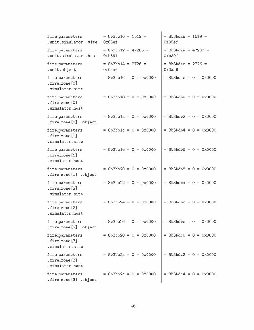
fire parameters.unit.simulator .site
= 8b3bb10 = 1519 =0x05ef
= 8b3bda8 = 1519 =0x05ef
fire parameters.unit.simulator .host
= 8b3bb12 = 47263 =0xb89f
= 8b3bdaa = 47263 =0xb89f
fire parameters.unit.object
= 8b3bb14 = 2726 =0x0aa6
= 8b3bdac = 2726 =0x0aa6
fire parameters.fire zone[0].simulator.site
= 8b3bb16 = 0 = 0x0000 = 8b3bdae = 0 = 0x0000
fire parameters.fire zone[0].simulator.host
= 8b3bb18 = 0 = 0x0000 = 8b3bdb0 = 0 = 0x0000
fire parameters.fire zone[0] .object
= 8b3bb1a = 0 = 0x0000 = 8b3bdb2 = 0 = 0x0000
fire parameters.fire zone[1].simulator.site
= 8b3bb1c = 0 = 0x0000 = 8b3bdb4 = 0 = 0x0000
fire parameters.fire zone[1].simulator.host
= 8b3bb1e = 0 = 0x0000 = 8b3bdb6 = 0 = 0x0000
fire parameters.fire zone[1] .object
= 8b3bb20 = 0 = 0x0000 = 8b3bdb8 = 0 = 0x0000
fire parameters.fire zone[2].simulator.site
= 8b3bb22 = 0 = 0x0000 = 8b3bdba = 0 = 0x0000
fire parameters.fire zone[2].simulator.host
= 8b3bb24 = 0 = 0x0000 = 8b3bdbc = 0 = 0x0000
fire parameters.fire zone[2] .object
= 8b3bb26 = 0 = 0x0000 = 8b3bdbe = 0 = 0x0000
fire parameters.fire zone[3].simulator.site
= 8b3bb28 = 0 = 0x0000 = 8b3bdc0 = 0 = 0x0000
fire parameters.fire zone[3].simulator.host
= 8b3bb2a = 0 = 0x0000 = 8b3bdc2 = 0 = 0x0000
fire parameters.fire zone[3] .object
= 8b3bb2c = 0 = 0x0000 = 8b3bdc4 = 0 = 0x0000
46
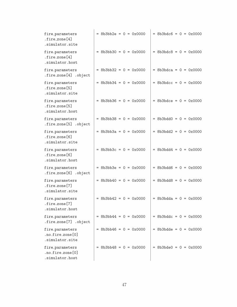
fire parameters.fire zone[4].simulator.site
= 8b3bb2e = 0 = 0x0000 = 8b3bdc6 = 0 = 0x0000
fire parameters.fire zone[4].simulator.host
= 8b3bb30 = 0 = 0x0000 = 8b3bdc8 = 0 = 0x0000
fire parameters.fire zone[4] .object
= 8b3bb32 = 0 = 0x0000 = 8b3bdca = 0 = 0x0000
fire parameters.fire zone[5].simulator.site
= 8b3bb34 = 0 = 0x0000 = 8b3bdcc = 0 = 0x0000
fire parameters.fire zone[5].simulator.host
= 8b3bb36 = 0 = 0x0000 = 8b3bdce = 0 = 0x0000
fire parameters.fire zone[5] .object
= 8b3bb38 = 0 = 0x0000 = 8b3bdd0 = 0 = 0x0000
fire parameters.fire zone[6].simulator.site
= 8b3bb3a = 0 = 0x0000 = 8b3bdd2 = 0 = 0x0000
fire parameters.fire zone[6].simulator.host
= 8b3bb3c = 0 = 0x0000 = 8b3bdd4 = 0 = 0x0000
fire parameters.fire zone[6] .object
= 8b3bb3e = 0 = 0x0000 = 8b3bdd6 = 0 = 0x0000
fire parameters.fire zone[7].simulator.site
= 8b3bb40 = 0 = 0x0000 = 8b3bdd8 = 0 = 0x0000
fire parameters.fire zone[7].simulator.host
= 8b3bb42 = 0 = 0x0000 = 8b3bdda = 0 = 0x0000
fire parameters.fire zone[7] .object
= 8b3bb44 = 0 = 0x0000 = 8b3bddc = 0 = 0x0000
fire parameters.no fire zone[0].simulator.site
= 8b3bb46 = 0 = 0x0000 = 8b3bdde = 0 = 0x0000
fire parameters.no fire zone[0].simulator.host
= 8b3bb48 = 0 = 0x0000 = 8b3bde0 = 0 = 0x0000
47
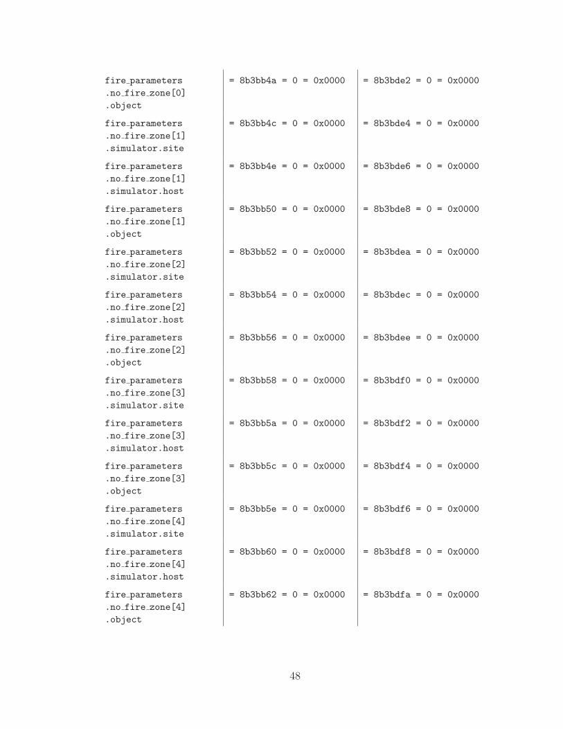
fire parameters.no fire zone[0].object
= 8b3bb4a = 0 = 0x0000 = 8b3bde2 = 0 = 0x0000
fire parameters.no fire zone[1].simulator.site
= 8b3bb4c = 0 = 0x0000 = 8b3bde4 = 0 = 0x0000
fire parameters.no fire zone[1].simulator.host
= 8b3bb4e = 0 = 0x0000 = 8b3bde6 = 0 = 0x0000
fire parameters.no fire zone[1].object
= 8b3bb50 = 0 = 0x0000 = 8b3bde8 = 0 = 0x0000
fire parameters.no fire zone[2].simulator.site
= 8b3bb52 = 0 = 0x0000 = 8b3bdea = 0 = 0x0000
fire parameters.no fire zone[2].simulator.host
= 8b3bb54 = 0 = 0x0000 = 8b3bdec = 0 = 0x0000
fire parameters.no fire zone[2].object
= 8b3bb56 = 0 = 0x0000 = 8b3bdee = 0 = 0x0000
fire parameters.no fire zone[3].simulator.site
= 8b3bb58 = 0 = 0x0000 = 8b3bdf0 = 0 = 0x0000
fire parameters.no fire zone[3].simulator.host
= 8b3bb5a = 0 = 0x0000 = 8b3bdf2 = 0 = 0x0000
fire parameters.no fire zone[3].object
= 8b3bb5c = 0 = 0x0000 = 8b3bdf4 = 0 = 0x0000
fire parameters.no fire zone[4].simulator.site
= 8b3bb5e = 0 = 0x0000 = 8b3bdf6 = 0 = 0x0000
fire parameters.no fire zone[4].simulator.host
= 8b3bb60 = 0 = 0x0000 = 8b3bdf8 = 0 = 0x0000
fire parameters.no fire zone[4].object
= 8b3bb62 = 0 = 0x0000 = 8b3bdfa = 0 = 0x0000
48
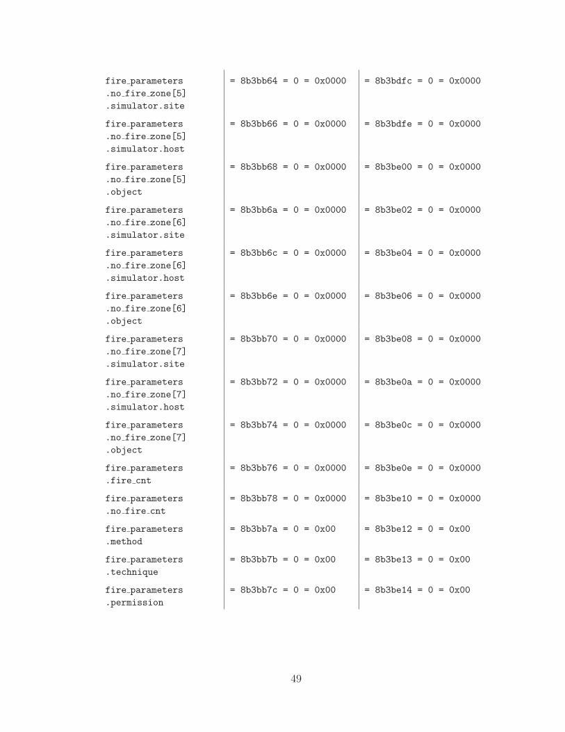
fire parameters.no fire zone[5].simulator.site
= 8b3bb64 = 0 = 0x0000 = 8b3bdfc = 0 = 0x0000
fire parameters.no fire zone[5].simulator.host
= 8b3bb66 = 0 = 0x0000 = 8b3bdfe = 0 = 0x0000
fire parameters.no fire zone[5].object
= 8b3bb68 = 0 = 0x0000 = 8b3be00 = 0 = 0x0000
fire parameters.no fire zone[6].simulator.site
= 8b3bb6a = 0 = 0x0000 = 8b3be02 = 0 = 0x0000
fire parameters.no fire zone[6].simulator.host
= 8b3bb6c = 0 = 0x0000 = 8b3be04 = 0 = 0x0000
fire parameters.no fire zone[6].object
= 8b3bb6e = 0 = 0x0000 = 8b3be06 = 0 = 0x0000
fire parameters.no fire zone[7].simulator.site
= 8b3bb70 = 0 = 0x0000 = 8b3be08 = 0 = 0x0000
fire parameters.no fire zone[7].simulator.host
= 8b3bb72 = 0 = 0x0000 = 8b3be0a = 0 = 0x0000
fire parameters.no fire zone[7].object
= 8b3bb74 = 0 = 0x0000 = 8b3be0c = 0 = 0x0000
fire parameters.fire cnt
= 8b3bb76 = 0 = 0x0000 = 8b3be0e = 0 = 0x0000
fire parameters.no fire cnt
= 8b3bb78 = 0 = 0x0000 = 8b3be10 = 0 = 0x0000
fire parameters.method
= 8b3bb7a = 0 = 0x00 = 8b3be12 = 0 = 0x00
fire parameters.technique
= 8b3bb7b = 0 = 0x00 = 8b3be13 = 0 = 0x00
fire parameters.permission
= 8b3bb7c = 0 = 0x00 = 8b3be14 = 0 = 0x00
49
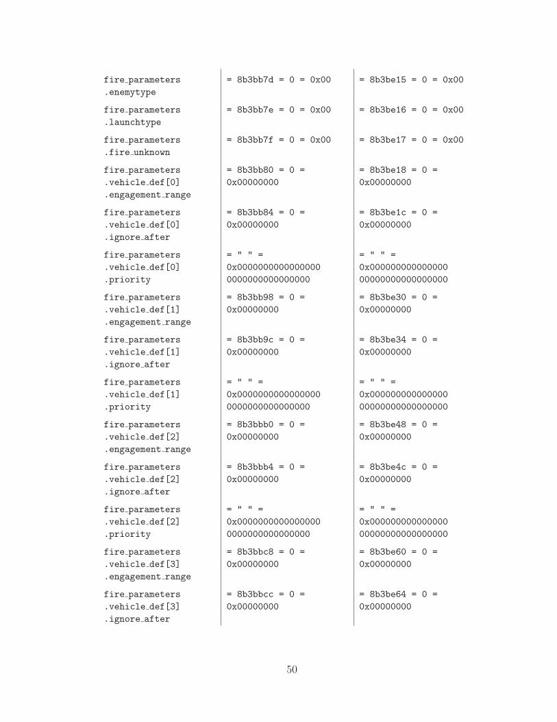
fire parameters.enemytype
= 8b3bb7d = 0 = 0x00 = 8b3be15 = 0 = 0x00
fire parameters.launchtype
= 8b3bb7e = 0 = 0x00 = 8b3be16 = 0 = 0x00
fire parameters.fire unknown
= 8b3bb7f = 0 = 0x00 = 8b3be17 = 0 = 0x00
fire parameters.vehicle def[0].engagement range
= 8b3bb80 = 0 =0x00000000
= 8b3be18 = 0 =0x00000000
fire parameters.vehicle def[0].ignore after
= 8b3bb84 = 0 =0x00000000
= 8b3be1c = 0 =0x00000000
fire parameters.vehicle def[0].priority
= " " =0x00000000000000000000000000000000
= " " =0x00000000000000000000000000000000
fire parameters.vehicle def[1].engagement range
= 8b3bb98 = 0 =0x00000000
= 8b3be30 = 0 =0x00000000
fire parameters.vehicle def[1].ignore after
= 8b3bb9c = 0 =0x00000000
= 8b3be34 = 0 =0x00000000
fire parameters.vehicle def[1].priority
= " " =0x00000000000000000000000000000000
= " " =0x00000000000000000000000000000000
fire parameters.vehicle def[2].engagement range
= 8b3bbb0 = 0 =0x00000000
= 8b3be48 = 0 =0x00000000
fire parameters.vehicle def[2].ignore after
= 8b3bbb4 = 0 =0x00000000
= 8b3be4c = 0 =0x00000000
fire parameters.vehicle def[2].priority
= " " =0x00000000000000000000000000000000
= " " =0x00000000000000000000000000000000
fire parameters.vehicle def[3].engagement range
= 8b3bbc8 = 0 =0x00000000
= 8b3be60 = 0 =0x00000000
fire parameters.vehicle def[3].ignore after
= 8b3bbcc = 0 =0x00000000
= 8b3be64 = 0 =0x00000000
50
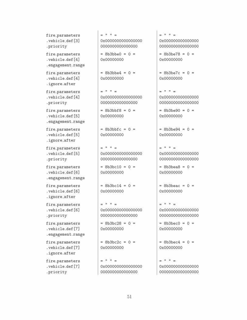
fire parameters.vehicle def[3].priority
= " " =0x00000000000000000000000000000000
= " " =0x00000000000000000000000000000000
fire parameters.vehicle def[4].engagement range
= 8b3bbe0 = 0 =0x00000000
= 8b3be78 = 0 =0x00000000
fire parameters.vehicle def[4].ignore after
= 8b3bbe4 = 0 =0x00000000
= 8b3be7c = 0 =0x00000000
fire parameters.vehicle def[4].priority
= " " =0x00000000000000000000000000000000
= " " =0x00000000000000000000000000000000
fire parameters.vehicle def[5].engagement range
= 8b3bbf8 = 0 =0x00000000
= 8b3be90 = 0 =0x00000000
fire parameters.vehicle def[5].ignore after
= 8b3bbfc = 0 =0x00000000
= 8b3be94 = 0 =0x00000000
fire parameters.vehicle def[5].priority
= " " =0x00000000000000000000000000000000
= " " =0x00000000000000000000000000000000
fire parameters.vehicle def[6].engagement range
= 8b3bc10 = 0 =0x00000000
= 8b3bea8 = 0 =0x00000000
fire parameters.vehicle def[6].ignore after
= 8b3bc14 = 0 =0x00000000
= 8b3beac = 0 =0x00000000
fire parameters.vehicle def[6].priority
= " " =0x00000000000000000000000000000000
= " " =0x00000000000000000000000000000000
fire parameters.vehicle def[7].engagement range
= 8b3bc28 = 0 =0x00000000
= 8b3bec0 = 0 =0x00000000
fire parameters.vehicle def[7].ignore after
= 8b3bc2c = 0 =0x00000000
= 8b3bec4 = 0 =0x00000000
fire parameters.vehicle def[7].priority
= " " =0x00000000000000000000000000000000
= " " =0x00000000000000000000000000000000
51
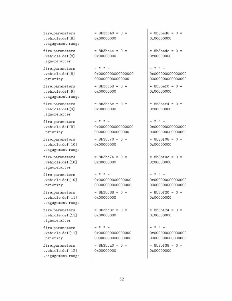
fire parameters.vehicle def[8].engagement range
= 8b3bc40 = 0 =0x00000000
= 8b3bed8 = 0 =0x00000000
fire parameters.vehicle def[8].ignore after
= 8b3bc44 = 0 =0x00000000
= 8b3bedc = 0 =0x00000000
fire parameters.vehicle def[8].priority
= " " =0x00000000000000000000000000000000
= " " =0x00000000000000000000000000000000
fire parameters.vehicle def[9].engagement range
= 8b3bc58 = 0 =0x00000000
= 8b3bef0 = 0 =0x00000000
fire parameters.vehicle def[9].ignore after
= 8b3bc5c = 0 =0x00000000
= 8b3bef4 = 0 =0x00000000
fire parameters.vehicle def[9].priority
= " " =0x00000000000000000000000000000000
= " " =0x00000000000000000000000000000000
fire parameters.vehicle def[10].engagement range
= 8b3bc70 = 0 =0x00000000
= 8b3bf08 = 0 =0x00000000
fire parameters.vehicle def[10].ignore after
= 8b3bc74 = 0 =0x00000000
= 8b3bf0c = 0 =0x00000000
fire parameters.vehicle def[10].priority
= " " =0x00000000000000000000000000000000
= " " =0x00000000000000000000000000000000
fire parameters.vehicle def[11].engagement range
= 8b3bc88 = 0 =0x00000000
= 8b3bf20 = 0 =0x00000000
fire parameters.vehicle def[11].ignore after
= 8b3bc8c = 0 =0x00000000
= 8b3bf24 = 0 =0x00000000
fire parameters.vehicle def[11].priority
= " " =0x00000000000000000000000000000000
= " " =0x00000000000000000000000000000000
fire parameters.vehicle def[12].engagement range
= 8b3bca0 = 0 =0x00000000
= 8b3bf38 = 0 =0x00000000
52
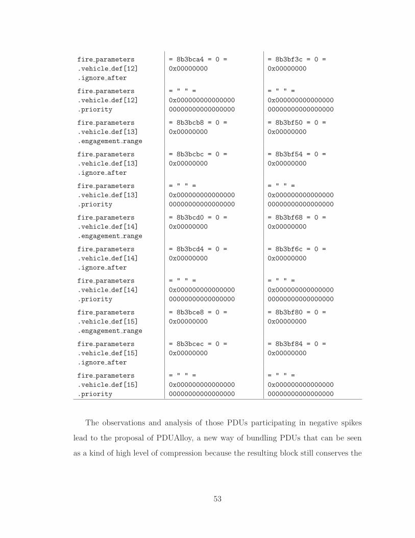
fire parameters.vehicle def[12].ignore after
= 8b3bca4 = 0 =0x00000000
= 8b3bf3c = 0 =0x00000000
fire parameters.vehicle def[12].priority
= " " =0x00000000000000000000000000000000
= " " =0x00000000000000000000000000000000
fire parameters.vehicle def[13].engagement range
= 8b3bcb8 = 0 =0x00000000
= 8b3bf50 = 0 =0x00000000
fire parameters.vehicle def[13].ignore after
= 8b3bcbc = 0 =0x00000000
= 8b3bf54 = 0 =0x00000000
fire parameters.vehicle def[13].priority
= " " =0x00000000000000000000000000000000
= " " =0x00000000000000000000000000000000
fire parameters.vehicle def[14].engagement range
= 8b3bcd0 = 0 =0x00000000
= 8b3bf68 = 0 =0x00000000
fire parameters.vehicle def[14].ignore after
= 8b3bcd4 = 0 =0x00000000
= 8b3bf6c = 0 =0x00000000
fire parameters.vehicle def[14].priority
= " " =0x00000000000000000000000000000000
= " " =0x00000000000000000000000000000000
fire parameters.vehicle def[15].engagement range
= 8b3bce8 = 0 =0x00000000
= 8b3bf80 = 0 =0x00000000
fire parameters.vehicle def[15].ignore after
= 8b3bcec = 0 =0x00000000
= 8b3bf84 = 0 =0x00000000
fire parameters.vehicle def[15].priority
= " " =0x00000000000000000000000000000000
= " " =0x00000000000000000000000000000000
The observations and analysis of those PDUs participating in negative spikes
lead to the proposal of PDUAlloy, a new way of bundling PDUs that can be seen
as a kind of high level of compression because the resulting block still conserves the
53
characteristics of a PDU, perhaps of a different type, and so it is subject to further
compressions. In fact, the proposed bundling does not remove the redundancy
within the same PDU: the fields filled with zeros in the basic (reference) PDU
will continue being the same length of zeros. Only the redundancy resulting from
the similarities between consecutive PDUs is removed. Therefore, other traditional
compression mechanisms are recommended after the bundling.
Replication is the converse procedure of bundling. Given a bundled block that
arrived to a destination, the individual PDUs have to be extracted or replicated
from it. Replication is independent of other data compression techniques because
it is targeted at the PDU level and the resulting traffic is of PDU type. Therefore,
even if there are no plans to modify the transport protocol in effect (by compressing
TCP/IP headers, for instance), the reduction of PDU packets to increment the
bandwidth availability by using replication is still applicable.
After running the simulator without using bundling, and collecting performance
statistics, it was observed that at 64 Kbps the generator in ground station could
not cope with the demanding traffic, and an increasing delay in timeliness to send
PDUs at the indicated timestamp started to build up. The proposed solution was to
bundle PDUs of the same type and length into longer ones, eliminating redundancy
in similar fields, as explained in the following section.
3.4.1 Mathematical Description of Bundling: PDUAlloy
The following definition is named PDUAlloy Bundling in this dissertation, and
is the base for the PDUAlloy algorithm of Section 4.4.
Given a set N = {1, 2, . . . , n} of indexes and two consecutive PDUs A =
(a1, a2, . . . , an) and B = (b1, b2, . . . , bn), where A and B are of the same type
54
and the ai and bi represent PDU fields, and a subset S ⊆ N such that ai = bi
for all i ∈ S, then the bundle of A and B is defined as the PDU A&B =
(a1, a2, . . . , an, ((bj, j)j∈N\S)). A is called the base PDU in the bundle. The definition
can be extended to any number of PDUs.
Example:
Given the PDUs: A = (a1, a2, a3, a4), B = (b1, b2, b3, b4), and C = (c1, c2, c3, c4),
such that a2 = b2 = c2, a3 = b3, a4 = c4, then the bundle A&B&C is the new
PDU
A&B&C = (a1, a2, a3, a4, ((b1, 1), (b4, 4)), ((c1, 1), (c3, 3)))
From the information contained in the shown n-tuple it is possible to reconstruct
the original PDUs A, B and C. Each component (bj, j) indicates that the value bj
replaces the field j in the base PDU. In a practical implementation, j could be a
pointer or an offset into the base PDU.
The above bundle will be called PDUAlloy because it acts like a metal alloy,
bundling PDUs based on their internal structure. It differs from other proposals
in several ways. First, the resulting bundle conserves the basic characteristics of
any other PDU and therefore, can be considered a new type of PDU subject to
further bundling and/or compression algorithms. In [BCL97] consecutive PDUs
are concatenated in a single packet even if their types are different, and field
redundancy is not eliminated. A delta-PDU encoding technique is mentioned
in [US95a] consisting of PDUs that carry changes respect to a reference PDU
initially given. In [WMS01] several bundling techniques generally applicable to
Web pages under the TCP/IP protocol suite are described, but none is specific
to the DIS protocol. A protocol called DIS-Lite developed by MaK Technologies
[Tay95, Tay96b, Tay96a, PW98] splits the Entity State PDU into static and dynamic
data PDUs, so that the static information is sent once and the changes (dynamic
55

PDUs) are subsequently sent as separate PDUs. According to [Ful96] by eliminating
redundancy, DIS-Lite can perform between 30 % and 70 % more efficiently than DIS.
DIS-Lite includes also several other improvements not related to the combination of
individual fields from a set of similar PDUs.
3.4.2 Implementation of PDU Bundling in the Simulator
After analyzing all of the PDUs in the log file for a given vignette, it was observed
that the type and the size of a PDU completely determine its internal field structure.
In other words, if PDUs A = (a1, a2, a3, . . . , an) and B = (b1, b2, . . . , bm) are such
that type(A) = type(B) and length(A) = length(B), then n = m and field type(ai) =
field type(bi) for all 1 ≤ i ≤ n, assuming that type, length and field type are functions
that return the type, the length in bytes, and the field type of a PDU, respectively.
If two PDUs are of the same type and length, they are called compatibles and are
candidates to be bundled.
The basic idea behind PDU bundling is that if consecutive PDUs of the same
type and length are scheduled within a predefined short time interval, then they can
be bundled and delivered as a single packet.
The pseudo-algorithm of PDU bundling is described as follows:
1. Wait until next PDU is ready for delivery. Let A be that PDU.
2. bundling = A. This is the first PDU (called base PDU) in the bundling.
3. Set timeout = maximum time A will wait in the bundle.
4. While (timeout not expired){
If next PDU is ready for delivery, let B be that PDU,
otherwise repeat the while-loop;
56
If A and B are compatible PDUs
{bundling = bundling & B; B = ∅;}else break the while-loop}
5. Send bundling PDUs through the network as a single packet.
6. If B = ∅ then repeat from step 1) else A = B and repeat from step 2).
This algorithm is called the Always-Wait algorithm because after processing a
PDU, the algorithm waits for the next one unless a timeout is detected. When the
next PDU is obtained, its type is checked and if it is different from the type of the
base PDU, the base PDU is sent and the time waited was wasted. It seems that if
there were a way to predict the type and length, or at least the type, of the next
PDU and the prediction indicates a type different form the type of the current base
PDU, then the current bundle could be sent immediately, saving the waiting time.
So, in the next paragraphs a variation of the above algorithm is introduced.
3.4.2.1 PDU Type prediction using a Neural Network
One way to predict the next PDU based on the recent history is by using a neural
network (NN) approach. A NN can learn sequences of PDU patterns and use them
as a basis for predicting the incoming type. In this research, we set up a gradient
descent NN that predicts the next type based on the types of the previous 48 PDUs.
Inorder not to complicate the simulator logic, the NN procedure was run offline, and
the results were incorporated into the PDU summary file. The NN predicted the
next PDU type with a certainty of near 70 %. Considering that there are near 27
different PDU types, the percentage is meaningful. If the NN prediction indicates
that the next PDU type is the same as the current one, a w (for wait) character is
appended offline to the summary file, otherwise an s (for send) is appended.
57

Due to the fact that the summary PDU files do not include the actual PDU
fields, it is impossible to determine the bundling resulting from two PDUs of the
same type and length because their fields cannot be compared and their differences
cannot be established. In this research, the comparison took place offline in the
pre-process stage using actual PDU fields, which resulted in three perfect prediction
offline methods, additionally to the in line neural network prediction. The perfect
prediction methods calculate the next PDU type with 100 % certainty because they
know all the sequence of PDUs in advance.
The first perfect prediction method considers the PDU type only, the second one
considers the type-and-length, and the last one considers the type-length-and-time.
Given any PDU, if the next one can be bundled to it because its type (method
1), and length (method 2), and timestamp (method 3) are equal, a W character
(meaning wait) is appended to the description of the current PDU in the summary
file, otherwise an S (send) is appended.
Figure 19 in Chapter 5 shows four characters at the end of each line containing the
S and W letters. The first character corresponds to the neural network prediction
and the rest correspond to each one of the perfect prediction methods. Only one
character is processed per run by the simulator and the omnetpp.ini file has been
set up to include the prediction method desired in each run.
Additionally to the four predictive methods already described, there are two
other ones called Always-Wait and Always-Send, obtained by assuming that one
column is filled all with either w or s characters, respectively.
Figure 17 shows the general algorithm used by each generator for sending PDUs
to the network. The abbreviations used in the figure are:
EOF end of file
bwt block waiting time, delayed incurred due to bundling
58
gt gap time, minimum separation between packets
rts ready-to-send message (future OMNeT event)
tt transmission time
∅ empty set
The generator is activated when it receives one of two possible messages from
the OMNeT kernel:
BlockTimeout: indicates that the oldest PDU in the current bundle has timed
out (bwt has elapsed), and therefore the generator must send it as soon as
possible, which means that if the generator is idle, the bundle can be sent
immediately, but if it is busy transmitting an older packet, then the current
bundle has to wait for the end of that transmission plus the gap time.
ReadyToSend (rts): indicates that the generator is not transmitting and is ready
to send a block that has timed out, or to get the next PDU from the summary
file. If during reading the next PDU the EOF condition arises, The the current
block of bundled PDUs is examined. If the block is empty, the generator stops,
otherwise it sets the conditions to proceed to send the bundle.
If a new PDU is successfully retrieved form the summary file, the generator
calculates its slack time. If the slack is positive, the generator schedules an rts
to be awaken at the PDU timestamp. If the slack is negative, the generator
is behind the schedule and proceeds to bundle the PDU to previous PDUs
already bundled, or to initiate a new bundle, or to send the current bundle
which is not compatible with this PDU and create a new bundle starting with
this PDU. In any case, the prediction character (W or S) is read and the
generator acts accordingly, either keeping the bundle in case of W, or sending
it in case of S.
59
If a bundle is performed, some time should be spent in the bundle operation itself.
In other words, it is not possible to process a PDU (read it and bundle it) in zero
time. Each schedule ready-to-send operation (Sched rts) includes some minimum
time (5µs) for the bundle operation. This time could be considered as generator
service time. The busy time is then computed as the transmission time(tt), plus
the gap time (gt), plus any generator service time if a bundling operation is carried
out.
60
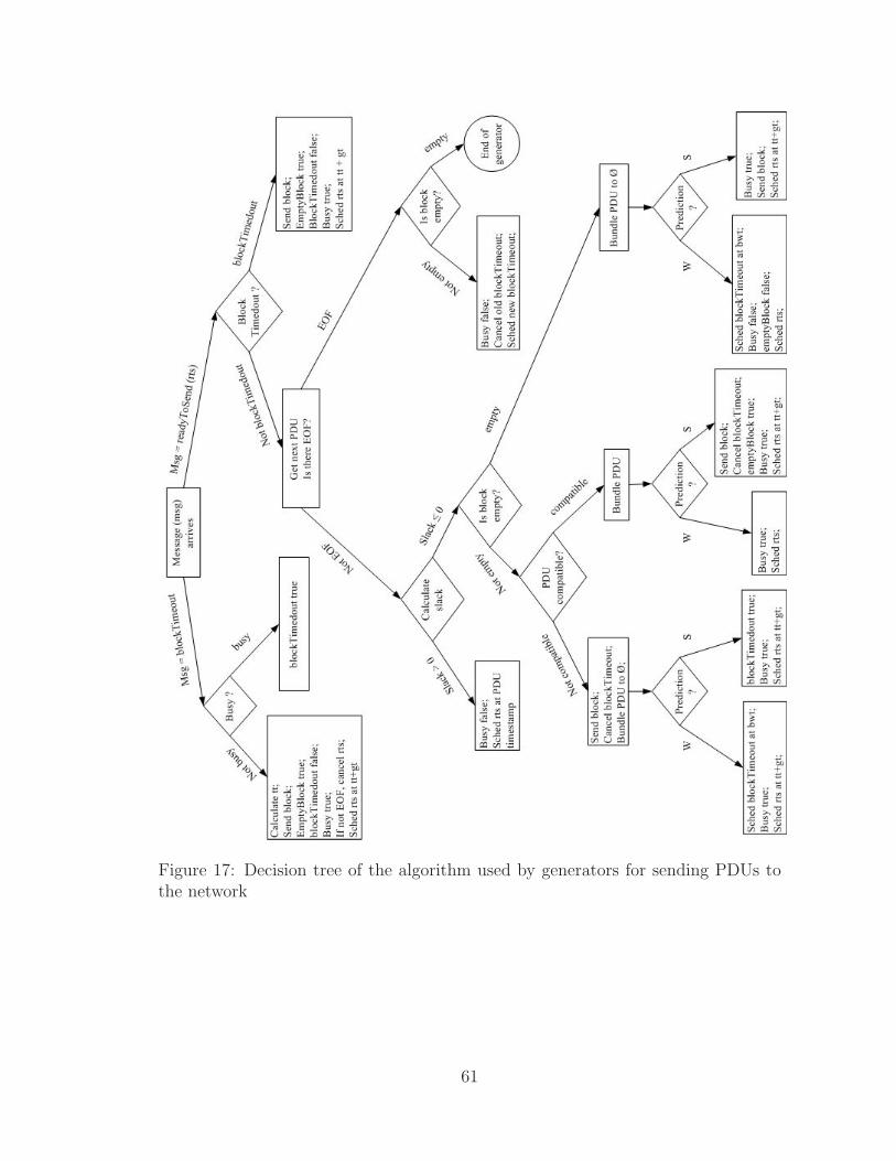
Figure 17: Decision tree of the algorithm used by generators for sending PDUs tothe network
61
CHAPTER 4
ACTIVE BUNDLING STRATEGIES
Bundling strategies are confronted with the decision of waiting for the next
packet to arrive and bundle it to the current block, or sending the current block and
start a new collection of packets from scratch. This type of decisions are typical of
online and offline algorithms.
4.1 Offline Bundling
Given a sequence σ of input data, in which the decision of processing each
individual data element applying one of several possible actions is taken with
complete knowledge of the whole sequence σ, constitutes an offline algorithm.
Applied to the network packets, each frame, message or PDU is an element of the
sequence, and the possible actions are bundling the incoming packet to the current
block, or sending the current block and start a new block. Because offline algorithms
know the complete packet sequence at the decision time, including the future packet
sequence, the best offline algorithm must take the optimal decision. A decision is
optimal if it minimizes some cost function. In the transmission of network packets,
the cost function could be the total latency time incurred by all the packets sent
from the origin to the final destination. Another cost function could be the absolute
value of the sum of all negative slack times when the PDUs are sent.
62
Symbolically, given a sequence σ = {PDU i}i=1,...,n of PDUs, where each packet
i is released and stamped at time Tstampi, and arrives at the final destination at
time Tarr i, then the cost function for the total latency of the travel time is:
CTtrav(σ) =n∑
i=1
(Tarr i − Tstampi) (4.1)
Similarly, if the simulator is reading PDUs from a summary log file, and each
PDU i is read for the first time at time Tread i, the cost function that measures the
absolute value of the total negative slack time is:
CTslack(σ) =n∑
i=1
H(Tread i − Tstampi)(Tstampi − Tread i) (4.2)
where H represents the Heaviside step function, H(x) = 1 if x > 0, 0 otherwise,
used to select only the negative slacks.
Offline algorithms are useful in many other computer-related areas. Most of the
database algorithms like sorting and searching files are offline. A recent example of
an offline algorithm for compressing data is given by Turpin in [TS02].
Offline algorithms are not supposed to be implemented in an actual real-time
simulation because obviously the messages to be produced in future times are not
known at the present simulation time. In simulation, the main application of
offline algorithms lies in the possibility of comparing them to the corresponding
online counterparts, with the purpose of asses online performances. A measure
of comparison of performance for online algorithms is the competitive ratio. A
competitive ratio of t > 0 means that the performance of an online algorithm is at
least a factor of 1/t of the performance achieved by the best offline algorithm. This
will be expanded in the next section.
Offline bundling is the process of taking decisions about to bundle or not
consecutive packets. Considering that after one packet has been sent, a certain
63
minimum time gap must elapse before sending the next packet, then the decision is
not trivial. If the first packet is sent immediately, the second one could be delayed
more than if the two packets are sent in a single bundle. This decisions are referred
to as the Packet Bundling Problem [FL02].
In the case of the OTB simulation, the offline bundling is carried out taking as
input the PDU log files produced by the OTB simulator, and not only the time
gaps, but also the type and the length of the PDUs are considered.
4.2 Online Bundling
General online and offline algorithms have been studied in the literature for a
long time [Kar92, FL02, FLN03, GHP03]. Karp defines these algorithms in the
following way.
An on-line algorithm is one that receives a sequence of requests and
performs an immediate action in response to each request. On-line
algorithms arise in any situation where decisions must be made and
resources allocated without knowledge of the future. The effectiveness
of an on-line algorithm may be measured by its competitive ratio, defined
as the worst-case ratio between its cost and that of a hypothetical off-line
algorithm which knows the entire sequence of requests in advance and
chooses its actions optimally (with minimum cost)[Kar92].
Online algorithms are characterized by a lack of knowledge about the future.
Phillips [PW99] indicates that the online algorithm receives each input and must
process it immediately, serving the sequence of requests one item at a time without
having explicit knowledge of the following inputs.
64
The performance of online deterministic algorithms is measured by its
competitive ratio when compared with the optimal offline algorithm. Ambuhl
[AGS01] defines this ratio in the following way. If σ is any input sequence,
A(σ) represents the cost function of an online algorithm A, and OPT (σ) is the
corresponding cost function of the optimal offline algorithm OPT , then A is called
c-competitive for a constant c if there exists a real number a such that for all input
sequences σ, it is true that:
A(σ) ≤ c · OPT (σ) + a (4.3)
If a = 0, then A is called strictly c-competitive. If A is a randomized algorithm,
equation 4.4 becomes:
E[A(σ)] ≤ c · OPT (σ) + a (4.4)
where E[A(σ)] represents the expected cost of algorithm A on the sequence σ.
The competitive ratio of an algorithm is defined as the infimum over all real
numbers c such that the algorithm is c-competitive [FLN03, GIS03].
4.3 Characteristics of Embedded Simulation TrafficImpacting Bundling
Several characteristics of the Embedded Simulation traffic are to be considered
for bundling purposes. The discussion here applies to PDUs generated under the
DIS protocol, although many of them are general enough to be valid under other
protocols as well.
65
4.3.1 The Simulation is a Real-Time Application
During the Embedded Simulation, the participants interact with each other in
real time. If one tank fires, or starts moving, or decelerates, all the other entities
should be informed of the event as soon as possible. This characteristic impacts
bundling in several aspects. First, the time a PDU waits for the upcoming PDU
creates a delay against the meaning of real time. Therefore, a small timeout should
be introduce to limit that waiting time. Second, not bundling PDUs could cause
that the following PDU will be delayed even more, due to the gap time that must
separate frames. Also, not bundling produces more traffic and longer router queues,
which finally goes in detriment of the real time properties.
The decision of bundling PDUs must consider the pros and cons of each
alternative. It is possible that for some environments bundling is not a necessity, for
example a scenario in which few sites are simulating a simple vignette, connected in
a LAN, not requiring a router.
4.3.2 There Is a High Percentage of ESPDUs
It is well documented that ES traffic contains 70% or more of Entity State PDUs.
Usually these ESPDUs are redundant and not urgent. For example, if a vehicle is not
moving, it still needs to send heartbeat ESPDUs at regular intervals. ESPDUs are
less harmed by waiting to be bundled than other PDUs of higher priority. Because
they are so abundant, bundling and compressing ESPDUs have a major impact on
the overall traffic decrease. However, in this research ESPDUs were not bundled in
the majority of cases because they did not participated in negative spikes as bursts
of consecutive ones, as po fire parameters did.
66
4.3.3 There Is a Low Percentage of High Priority PDUs
Some high priority PDUs like fire and detonation occur in short bursts, but
they are usually sent at the same time, creating negative slack spikes that attempt
against the real time approach. If the bundling operation is not time-consuming and
the waiting timeout is selected appropriately, bundling a sequence of consecutive
PDU and sending a single block could take less time than sending the individual
PDUs without bundling them. For instance, if a PDU is 512 bytes long and the
bandwidth is 64 Kbps, the transmission time of one single PDU is 64 milliseconds,
while bundling several PDUs could take less than one millisecond.
4.3.4 High Levels of Redundancy
PDUs contain lots of redundancy, both inside each PDU and across PDUs. As
a sample, the PDUs listed in Table 2 contain zeroes in the majority of fields, and
just two differences from one PDU to the other. Bundling and compression can take
advantage of this high redundancy. For example, the proposed algorithm PDUAlloy
would append only the two fields containing the differences in the second PDU of the
table to the first one. Other bundling algorithms also profit from this redundancy,
like those based on sending delta PDUs.
4.3.5 PDU Internal Structure
PDUs have a definite structure made up of fields of different sizes, that are
determined by the type and length of the PDUs. This characteristic allows the
comparison of PDUs at the field level, which facilitates the extraction of the
67
differences. Determination of the PDU structure based on the type and the length
allows a fast comparison among PDUs for algorithms like PDUAlloy.,
4.3.6 PDUs Are Broadcasted
In the DIS protocol, PDUs are broadcasted. This characteristic simplifies the
PDU header since a particular destination is not needed. All the PDUs in a bundle
are to be delivered to the same recipients.
4.3.7 Slow Connections Favor Bundling
The slower the connections, the better the bundling. If a connection is slow,
bundling and compression becomes more necessary. In slow connections, gap times
are larger, and so the penalty for not bundling the next PDU. Also, a slow bandwidth
shows more negative slack times during transmission, causing bottlenecks and long
queues. As an example, in the MR1 vignette the satellite connection introduces a
propagation delay of about 0.25 seconds, much higher than the time gap required
to separate frames during transmission. Therefore, bundling of high priority PDUs
like po fire parameters is worth.
4.3.8 PDU Bursts Scheduled at Once
Bursts of PDUs timestamped at the same or almost the same time encourages
bundling, because not doing it causes a large negative slack spike, or bottleneck, at
the transmitting site that delays the following PDUs.
68

4.4 PDUAlloy Bundling Model
The proposal of the algorithm PDUAlloy involves decisions about to bundle or
not two consecutive PDUs. Three variables can be considered in this algorithm: the
type, the length and the timestamp of each PDU. Observations taken from PDUs
participating in negative spikes indicate that if the type and the length of consecutive
PDUs are the same, they are compatible and can be bundled according to the
definition in Section 3.4.1.
4.4.1 Overview
The online algorithms proposed try to identify compatible PDUs P1 and P2 that
can be bundled in a block B = P1&P2. A requirement is that the two PDUs should
have the same type and length. But because P2 has not arrived by the time P1 is
being processed, the generating site must decide whether it will send P1 immediately,
or wait for P2. Chances are that P2 will not be compatible with P1. If the generator
could predict the type and the length of P2, then the prediction could be used in
the decision process. It is more difficult to predict both, type and length, than only
one variable. For decisions based on one variable only, the type is preferred because
it discriminates better among PDUs.
A neural network approach was used to predict the type only, as indicated
in Section 3.4.2.1. Besides that, other non-predictive online algorithms were
proposed: Always-Wait and Always-Send. The former takes the decision of wait
all the time, using a timeout of 100 milliseconds, much less than the 0.25 second
delay of the satellite link. The latter never waits. It sends the PDU as soon as the
time gap has elapsed, actually not bundling PDUs.
69
Considering the functions:
type(PDU ) (4.5)
length(PDU )
timestamp(PDU )
compatible(PDU 1,PDU 2)
that return the type, length and timestamp of any PDU, as well as the true value
of PDU compatibility, respectively, then three offline bundling algorithms can be
defined: Type, Type+Length and Type+Length+Time, as explained next.
4.4.2 Type
If (Pi)i=1...n is the sequence of PDUs to be transmitted from some site, then
the Type offline algorithm takes its bundling decision based on the type of the
PDUs. Using the notation of Section 3.4.1, if the block B already contains some
PDUs, being Pk the first one (base PDU), then Pj will be bundled: B = B&Pj if
type(Pj) = type(Pk) and compatible(Pj, Pk) is true.
In words, if the two PDUs bear the same type, then their compatibility is
analyzed, and if a successful comparison results, they are bundled.
4.4.3 Type+Length
The Type+Length offline algorithm takes its bundling decision based on the type
and length of the PDUs. Given the sequence (Pi)i=1...n of PDUs, and assuming the
the block B contains the base PDU Pk, then a new PDU Pj will be bundled in
70
the sense of B = B&Pj if type(Pj) = type(Pk), and length(Pj) = length(Pk) and
compatible(Pj, Pk) is true.
In words, if the two PDUs bear the same type and length, then their compatibility
is analyzed, and if a successful comparison results, they are bundled.
4.4.4 Type+Length+Time
This last algorithm called Type+Length+Time is similar to the previous
ones, except that it includes an extra condition for bundling: timestamp(Pj) =
timestamp(Pk). The condition looks very restrictive because it asks for an exact
match of timestamp in both PDUs. If two PDUs were scheduled with a time
difference of one single nanosecond, the offline algorithm will not bundle them.
In practice, it has been observed hundreds of PDUs scheduled exactly at the same
time. Therefore, the purpose of this algorithm is to evaluate the impact of bundling
just those PDUs.
71

CHAPTER 5
EMBEDDED SIMULATION TRAFFIC
ANALYSIS
5.1 Processing Flow and Sequencing
The simulator was run on data collected from several vignettes. Initially, a
vignette developed by Hubert Bahr for his PhD research under the advice of Dr.
Ronald DeMara was used. This vignette contained PDUs sent by one single entity.
A second simulation was run on a vignette containing two senders. Because of
its simplicity, this vignette, as well as the previous one, were used mainly to test
the simulator and to have some insight about the preprocessing that had to be
performed on the input data previous to the simulation phase.
The most important results in this research come from the MR1 vignette
described in Appendix A, which includes 6 senders. Four sets of simulations were
performed on it, varying the assignment of senders to computer nodes. Additionally,
simulations were run to observe the effect of applying PDU bundling, as well as the
usage of the Head of Line (HOL) priority in router queues.
5.2 Input Data and AWK preprocessing
The input data to this model comes from the OTB logger. After setting up
a particular vignette, OTB runs it and the logger records all the Protocol Data
72

Units into an output file that is later converted to ASCII text. OTB does not
generate regular PDUs, but Persistent Object PDUs (PO PDUs) that are a subclass
of the general category of PDUs. PDU formats are defined in the IEEE Standards
[IEE95a], [IEE95b], [IEE96] and [IEE98]. Although PO PDUs have a somewhat
different format as compared to regular PDUs, a considerable degree of similarity
exists that allows the application of the IEEE standards to PO PDUs in order to
extract information about the type, length and timestamp of each message.
The raw data collected by the OTB logger is not directly used as input to the
simulator due to the large size of the file (265 Mb for the MR1 vignette) and to the
amounts of data stored therein, which are unnecessary for the simulation. The log is
an ASCII file containing the descriptions of all the transmitted PO PDUs. Figures
20 and 21 display samples of the raw log.
When OTB ends processing the vignette, an awk program (see Appendix C)
parses the ASCII file and collects only those PDU variables required during the
simulation (type, length and timestamp) into a summary PDU file, along with two
newly created counters. One counter represents a local PDU ID for the generating
site, and the other is a global ID from among all the participating sites.
The OTB logger does not save PDUs in strict ascending order of timestamp
within the input files. In the logged files collected from running the vignettes there
were found sequences of 40 or more PDUs bearing exactly the same timestamp, as
well as cases of PDUs stored in reverse chronological order. Due to these anomalies,
the PDU files are sorted chronologically previous to running the awk program that
assigns the local and global IDs, keeping the original relative order for records having
the same timestamp. Figure 18 depicts a general view of the steps involved in the
simulation process.
The awk parser creates a separate file for each different transmitting site found,
and names it datan.txt, where n is the site ID. Each datan.txt file contains
73

Figure 18: Overview of the simulation process
summaries of all the PDUs generated by site n. Then, during the simulation, each
generator n reads in the corresponding PDU summary file datan.txt created out
of OTB logged data. A sample of the resulting files datan.txt is shown in Figure
19.
The information listed in Figure 19 is interpreted as follows from left to right:
hexadecimal timestamp, PDU length in bytes, separator “—”, decimal timestamp,
local PDU ID equivalent to the current position of the PDU within the file, PDU
type surrounded by angle brackets, global PDU ID, and the four letters S and W
already explained in Section 3.4.2.1.
In the DIS protocol timestamps are stored in 32 bits. In order to convert
timestamps into decimal, each unit of the unsigned integer value stored in the
leftmost 31 bits represents 1/(231 − 1) of an hour, giving the timestamp a resolution
of less than 0.5 nanoseconds. The rightmost bit of the timestamp is a flag that
indicates whether the time is relative to an arbitrary initial time, or absolute (UTC
time). For example, the value in the hex timestamp 0x4f690c7a corresponds to
4f690c7a/2 = 27B4863D = 666142269 units in decimal, and 666142269/(231−1) =
0.31019666 hours =: 18 : 36.707, as indicated in the sample file of Figure 19.
74
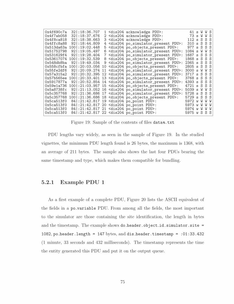
0x4f690c7a 32|:18:36.707 1 <dis204 acknowledge PDU>: 41 s W W S0x4f7ab058 32|:18:37.676 2 <dis204 acknowledge PDU>: 73 s W W S0x4f8ca818 32|:18:38.663 3 <dis204 acknowledge PDU>: 112 s S S S0x4ffc8a88 92|:18:44.809 4 <dis204 po_simulator_present PDU>: 310 s S S S0x513da63a 100|:19:02.448 5 <dis204 po_objects_present PDU>: 977 s S S S0x51752798 92|:19:05.497 6 <dis204 po_simulator_present PDU>: 1084 s W W S0x531629f4 92|:19:28.404 7 <dis204 po_simulator_present PDU>: 1687 s S S S0x53617074 100|:19:32.539 8 <dis204 po_objects_present PDU>: 1868 s S S S0x548db8ba 92|:19:49.034 9 <dis204 po_simulator_present PDU>: 2365 s S S S0x558cfbfa 100|:20:03.056 10 <dis204 po_objects_present PDU>: 2805 s S S S0x55fe2df6 92|:20:09.274 11 <dis204 po_simulator_present PDU>: 3000 s W W S0x57a315a2 92|:20:32.395 12 <dis204 po_simulator_present PDU>: 3717 s S S S0x57b565ee 100|:20:33.401 13 <dis204 po_objects_present PDU>: 3768 s S S S0x5917877a 92|:20:52.854 14 <dis204 po_simulator_present PDU>: 4393 s S S S0x59e1a736 100|:21:03.957 15 <dis204 po_objects_present PDU>: 4721 s S S S0x5a8738fc 92|:21:13.052 16 <dis204 po_simulator_present PDU>: 5039 s W W S0x5c357768 92|:21:36.686 17 <dis204 po_simulator_present PDU>: 5728 s S S S0x5c357768 100|:21:36.686 18 <dis204 po_objects_present PDU>: 5729 s S S S0x5ca513f0 84|:21:42.817 19 <dis204 po_point PDU>: 5972 w W W W0x5ca513f0 84|:21:42.817 20 <dis204 po_point PDU>: 5973 w W W W0x5ca513f0 84|:21:42.817 21 <dis204 po_point PDU>: 5974 w W W W0x5ca513f0 84|:21:42.817 22 <dis204 po_point PDU>: 5975 w S S S
Figure 19: Sample of the contents of files datan.txt
PDU lengths vary widely, as seen in the sample of Figure 19. In the studied
vignettes, the minimum PDU length found is 26 bytes, the maximum is 1368, with
an average of 211 bytes. The sample also shows the last four PDUs bearing the
same timestamp and type, which makes them compatible for bundling.
5.2.1 Example PDU 1
As a first example of a complete PDU, Figure 20 lists the ASCII equivalent of
the fields in a po variable PDU. From among all the fields, the most important
to the simulator are those containing the site identification, the length in bytes
and the timestamp. The example shows do header.object id.simulator.site =
1082, po header.length = 147 bytes, and dis header.timestamp = :01:33.432
(1 minute, 33 seconds and 432 milliseconds). The timestamp represents the time
the entity generated this PDU and put it on the output queue.
75
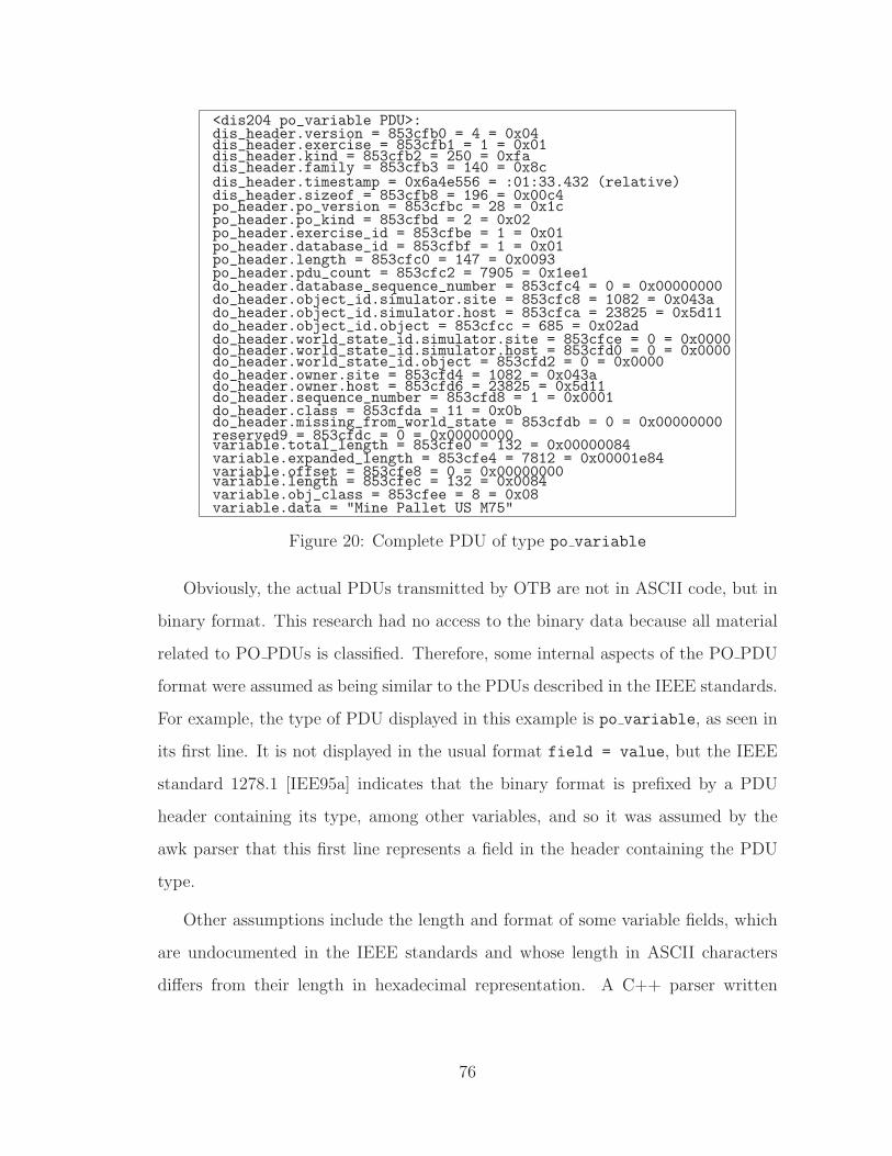
<dis204 po_variable PDU>:dis_header.version = 853cfb0 = 4 = 0x04dis_header.exercise = 853cfb1 = 1 = 0x01dis_header.kind = 853cfb2 = 250 = 0xfadis_header.family = 853cfb3 = 140 = 0x8cdis_header.timestamp = 0x6a4e556 = :01:33.432 (relative)dis_header.sizeof = 853cfb8 = 196 = 0x00c4po_header.po_version = 853cfbc = 28 = 0x1cpo_header.po_kind = 853cfbd = 2 = 0x02po_header.exercise_id = 853cfbe = 1 = 0x01po_header.database_id = 853cfbf = 1 = 0x01po_header.length = 853cfc0 = 147 = 0x0093po_header.pdu_count = 853cfc2 = 7905 = 0x1ee1do_header.database_sequence_number = 853cfc4 = 0 = 0x00000000do_header.object_id.simulator.site = 853cfc8 = 1082 = 0x043ado_header.object_id.simulator.host = 853cfca = 23825 = 0x5d11do_header.object_id.object = 853cfcc = 685 = 0x02addo_header.world_state_id.simulator.site = 853cfce = 0 = 0x0000do_header.world_state_id.simulator.host = 853cfd0 = 0 = 0x0000do_header.world_state_id.object = 853cfd2 = 0 = 0x0000do_header.owner.site = 853cfd4 = 1082 = 0x043ado_header.owner.host = 853cfd6 = 23825 = 0x5d11do_header.sequence_number = 853cfd8 = 1 = 0x0001do_header.class = 853cfda = 11 = 0x0bdo_header.missing_from_world_state = 853cfdb = 0 = 0x00000000reserved9 = 853cfdc = 0 = 0x00000000variable.total_length = 853cfe0 = 132 = 0x00000084variable.expanded_length = 853cfe4 = 7812 = 0x00001e84variable.offset = 853cfe8 = 0 = 0x00000000variable.length = 853cfec = 132 = 0x0084variable.obj_class = 853cfee = 8 = 0x08variable.data = "Mine Pallet US M75"
Figure 20: Complete PDU of type po variable
Obviously, the actual PDUs transmitted by OTB are not in ASCII code, but in
binary format. This research had no access to the binary data because all material
related to PO PDUs is classified. Therefore, some internal aspects of the PO PDU
format were assumed as being similar to the PDUs described in the IEEE standards.
For example, the type of PDU displayed in this example is po variable, as seen in
its first line. It is not displayed in the usual format field = value, but the IEEE
standard 1278.1 [IEE95a] indicates that the binary format is prefixed by a PDU
header containing its type, among other variables, and so it was assumed by the
awk parser that this first line represents a field in the header containing the PDU
type.
Other assumptions include the length and format of some variable fields, which
are undocumented in the IEEE standards and whose length in ASCII characters
differs from their length in hexadecimal representation. A C++ parser written
76
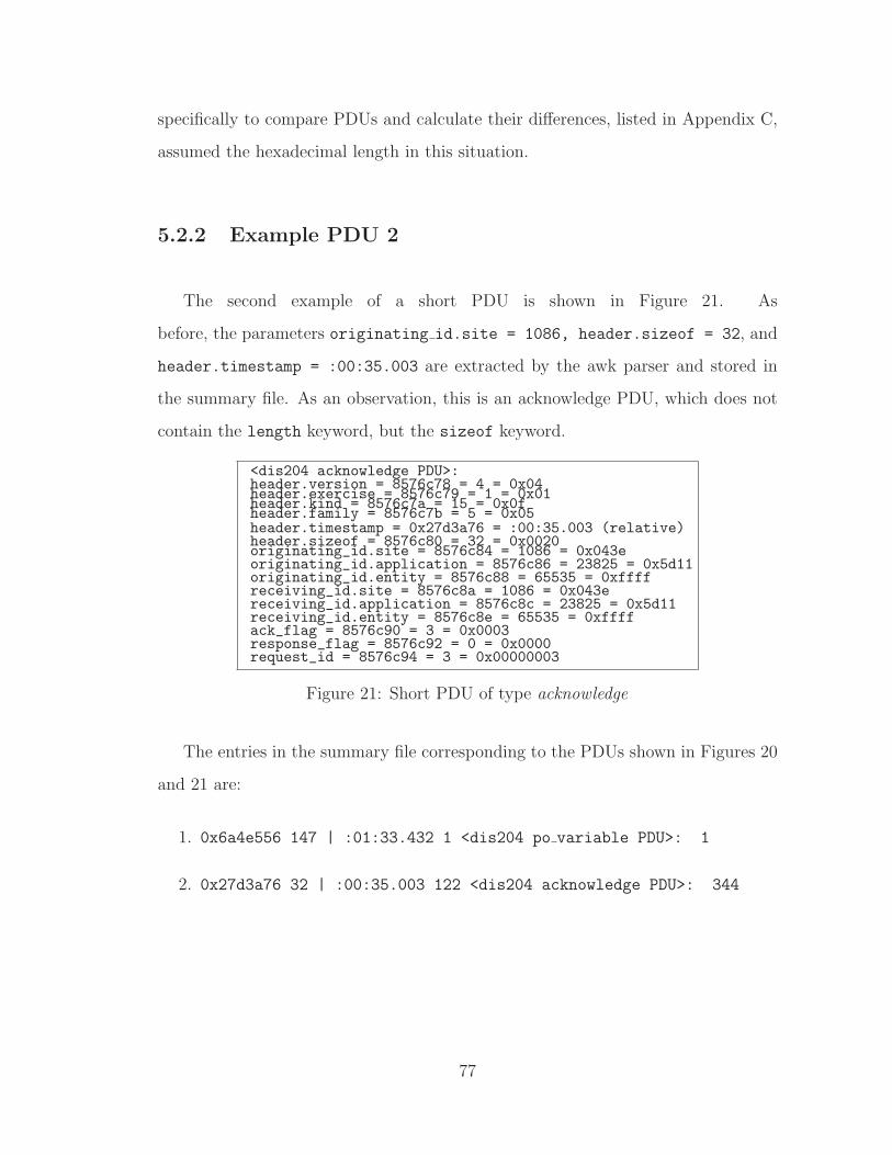
specifically to compare PDUs and calculate their differences, listed in Appendix C,
assumed the hexadecimal length in this situation.
5.2.2 Example PDU 2
The second example of a short PDU is shown in Figure 21. As
before, the parameters originating id.site = 1086, header.sizeof = 32, and
header.timestamp = :00:35.003 are extracted by the awk parser and stored in
the summary file. As an observation, this is an acknowledge PDU, which does not
contain the length keyword, but the sizeof keyword.
<dis204 acknowledge PDU>:header.version = 8576c78 = 4 = 0x04header.exercise = 8576c79 = 1 = 0x01header.kind = 8576c7a = 15 = 0x0fheader.family = 8576c7b = 5 = 0x05header.timestamp = 0x27d3a76 = :00:35.003 (relative)header.sizeof = 8576c80 = 32 = 0x0020originating_id.site = 8576c84 = 1086 = 0x043eoriginating_id.application = 8576c86 = 23825 = 0x5d11originating_id.entity = 8576c88 = 65535 = 0xffffreceiving_id.site = 8576c8a = 1086 = 0x043ereceiving_id.application = 8576c8c = 23825 = 0x5d11receiving_id.entity = 8576c8e = 65535 = 0xffffack_flag = 8576c90 = 3 = 0x0003response_flag = 8576c92 = 0 = 0x0000request_id = 8576c94 = 3 = 0x00000003
Figure 21: Short PDU of type acknowledge
The entries in the summary file corresponding to the PDUs shown in Figures 20
and 21 are:
1. 0x6a4e556 147 | :01:33.432 1 <dis204 po variable PDU>: 1
2. 0x27d3a76 32 | :00:35.003 122 <dis204 acknowledge PDU>: 344
77
5.3 Parameters Analyzed
For each experiment, two types of analyses were performed. The first one can
be called independent or offline because it takes place before running the simulator.
The second one corresponds to the results obtained by running the simulator.
5.3.1 Independent Analysis
This analysis is subdivided into 2 categories: distribution and assignment of
PDUs, and minimum bandwidth requirements.
5.3.1.1 Distribution and Assignment of PDUs
This is a frequency distribution of all the types of PDUs involved in the
experiment, as well as the assignment of computer sites mentioned in the PDUs to
simulated generators in computer nodes. The distribution gives information about
the sites with more activity that can be taken into account for a better strategic
assignment to computer nodes.
5.3.1.2 Minimum Bandwidth Requirements
An awk program was written to merge the PDUs of all the sites in one single
stream of data sorted according to their timestamps. Then, another program
calculates the required bandwidth at specific time intervals (2 seconds) without
performing any simulation. Computing the bandwidth based on a single data stream
is justified by the fact that all PDUs are broadcasted, and so any listening site will
78
have to receive the PDUs from all the generating sites as one single stream of
data. Due to traffic changes in time, different minimum instant bandwidths over
time are required. Instant bandwidth is computed as the ratio of volume of data
transmitted to the time interval allotted among consecutive PDUs. No overheads
like retransmissions, packet losses, or collisions are considered in the calculation
of the bandwidth. However, a time gap separation of 50 microseconds between
consecutive PDUs was included in accordance with the IEEE Std. 802.11 [IEE97].
Therefore, the resulting minimum bandwidth should be seen as an absolute lower
bound for the actual bandwidth. The awk script in Section C.2 of Appendix C
calculates the bandwidth for each set of PDUs.
The mathematical definition of the minimum instant bandwidth concept follows.
Let all the PDUs in the simulation be sorted in ascending order of timestamp and
numbered PDU1, . . ., PDUn. The length in bytes and the timestamp in seconds of
PDUi are represented, respectively, by Li and Ti. Let g be the minimum separating
time gap between PDUs. The minimum instant bandwidth is defined for those
time intervals of minimum length greater than or equal to S seconds, delimited by
timestamps Ti that meet some conditions. Specifically, given a pair of timestamps
Ta and Tb as close as possible to each other such that the following conditions hold:
Tb − Ta ≥ S (5.1)
Tb − Ti − (b − i)g > 0, ∀ i : a ≤ i < b (5.2)
then, the average bandwidth Bi for the time subinterval [Ti − Tb) is calculated as:
Bi =
b−1∑
j=i
8Lj
Tb − Ti − (b − i)g(5.3)
79
and the minimum instant bandwidth for the interval [Ta, Tb] is given by:
B = maxa≤ i < b
{Bi} (5.4)
It should be noted that the time interval [Ti − Tb) includes PDUi and does not
include PDUb. Equation 5.1 indicates that the time interval must have a minimum
length of S seconds, for a given constant S selected a priori. Equation 5.2 says
that the remaining time from Ti to Tb should be enough to accommodate all the
gaps between PDUs and still have some room for the transmission of bytes. The
average bandwidth for the interval [Ti − Tb) is the ratio of the total number of bits
transmitted to the remaining time in the interval once the gaps have been deducted,
as stated in Equation 5.3. Finally, given that the bandwidth for the whole interval
[Ta, Tb] is constant, it should not be less than any individual average bandwidth
Bi. Therefore, Equation 5.4 takes the maximum of all the Bi and considers it the
minimum bandwidth required.
5.3.2 Analysis of Simulation Results
This analysis is subdivided into 4 categories:
a) Slack Time Analysis. Statistics about the slack time of all the PDUs
generated at a particular site are graphed and discussed. The slack time
Tslack of a given PDU is defined as the difference between its timestamp and
the current simulator time at the moment the PDU is read from the summary
input file. In symbols, if Tstamp represents the timestamp of a PDU and
Tread represents the time when the PDU was read, then
Tslack = Tstamp − Tread (5.5)
80
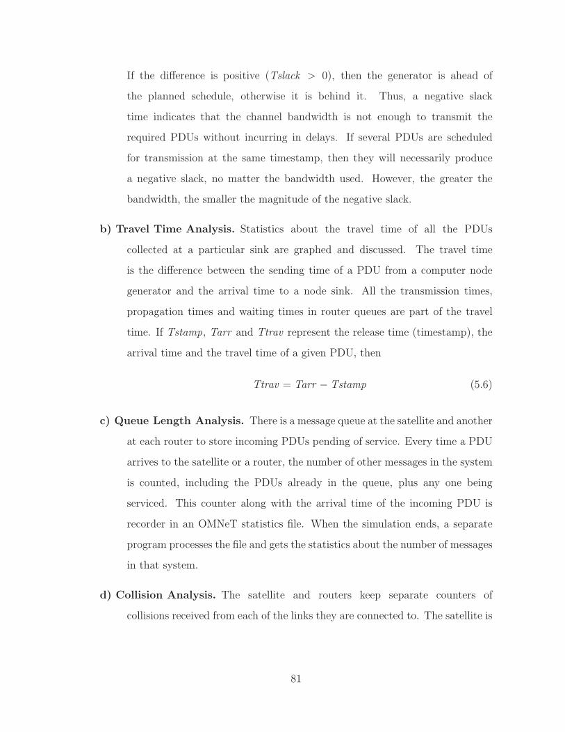
If the difference is positive (Tslack > 0), then the generator is ahead of
the planned schedule, otherwise it is behind it. Thus, a negative slack
time indicates that the channel bandwidth is not enough to transmit the
required PDUs without incurring in delays. If several PDUs are scheduled
for transmission at the same timestamp, then they will necessarily produce
a negative slack, no matter the bandwidth used. However, the greater the
bandwidth, the smaller the magnitude of the negative slack.
b) Travel Time Analysis. Statistics about the travel time of all the PDUs
collected at a particular sink are graphed and discussed. The travel time
is the difference between the sending time of a PDU from a computer node
generator and the arrival time to a node sink. All the transmission times,
propagation times and waiting times in router queues are part of the travel
time. If Tstamp, Tarr and Ttrav represent the release time (timestamp), the
arrival time and the travel time of a given PDU, then
Ttrav = Tarr − Tstamp (5.6)
c) Queue Length Analysis. There is a message queue at the satellite and another
at each router to store incoming PDUs pending of service. Every time a PDU
arrives to the satellite or a router, the number of other messages in the system
is counted, including the PDUs already in the queue, plus any one being
serviced. This counter along with the arrival time of the incoming PDU is
recorder in an OMNeT statistics file. When the simulation ends, a separate
program processes the file and gets the statistics about the number of messages
in that system.
d) Collision Analysis. The satellite and routers keep separate counters of
collisions received from each of the links they are connected to. The satellite is
81
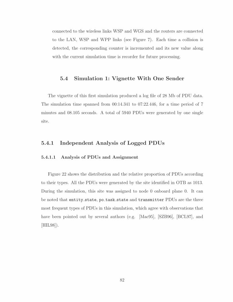
connected to the wireless links WSP and WGS and the routers are connected
to the LAN, WSP and WPP links (see Figure 7). Each time a collision is
detected, the corresponding counter is incremented and its new value along
with the current simulation time is recorder for future processing.
5.4 Simulation 1: Vignette With One Sender
The vignette of this first simulation produced a log file of 28 Mb of PDU data.
The simulation time spanned from 00:14.341 to 07:22.446, for a time period of 7
minutes and 08.105 seconds. A total of 5940 PDUs were generated by one single
site.
5.4.1 Independent Analysis of Logged PDUs
5.4.1.1 Analysis of PDUs and Assignment
Figure 22 shows the distribution and the relative proportion of PDUs according
to their types. All the PDUs were generated by the site identified in OTB as 1013.
During the simulation, this site was assigned to node 0 onboard plane 0. It can
be noted that entity state, po task state and transmitter PDUs are the three
most frequent types of PDUs in this simulation, which agree with observations that
have been pointed out by several authors (e.g. [Mac95], [SZB96], [BCL97], and
[HIL98]).
82
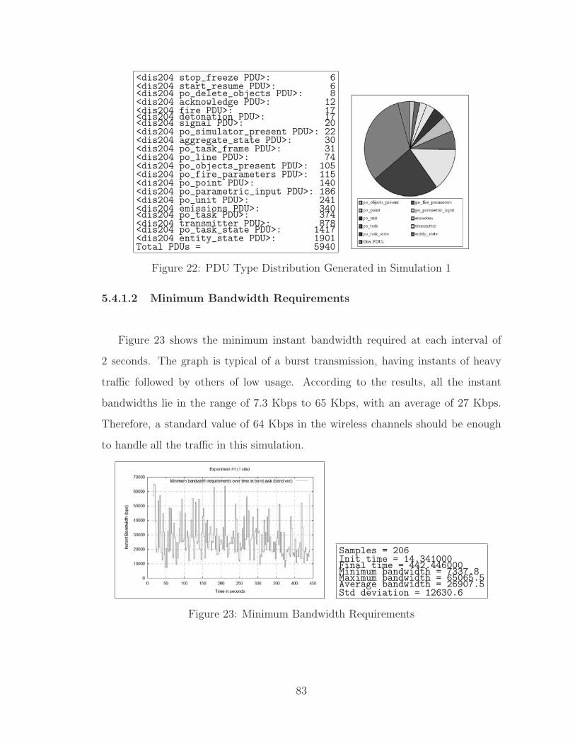
<dis204 stop_freeze PDU>: 6<dis204 start_resume PDU>: 6<dis204 po_delete_objects PDU>: 8<dis204 acknowledge PDU>: 12<dis204 fire PDU>: 17<dis204 detonation PDU>: 17<dis204 signal PDU>: 20<dis204 po_simulator_present PDU>: 22<dis204 aggregate_state PDU>: 30<dis204 po_task_frame PDU>: 31<dis204 po_line PDU>: 74<dis204 po_objects_present PDU>: 105<dis204 po_fire_parameters PDU>: 115<dis204 po_point PDU>: 140<dis204 po_parametric_input PDU>: 186<dis204 po_unit PDU>: 241<dis204 emissions PDU>: 340<dis204 po_task PDU>: 374<dis204 transmitter PDU>: 878<dis204 po_task_state PDU>: 1417<dis204 entity_state PDU>: 1901Total PDUs = 5940
Figure 22: PDU Type Distribution Generated in Simulation 1
5.4.1.2 Minimum Bandwidth Requirements
Figure 23 shows the minimum instant bandwidth required at each interval of
2 seconds. The graph is typical of a burst transmission, having instants of heavy
traffic followed by others of low usage. According to the results, all the instant
bandwidths lie in the range of 7.3 Kbps to 65 Kbps, with an average of 27 Kbps.
Therefore, a standard value of 64 Kbps in the wireless channels should be enough
to handle all the traffic in this simulation.
Samples = 206Init time = 14.341000Final time = 442.446000Minimum bandwidth = 7337.8Maximum bandwidth = 65065.5Average bandwidth = 26907.5Std deviation = 12630.6
Figure 23: Minimum Bandwidth Requirements
83
5.4.2 Slack Time
Figure 24 shows that negative slacks are not detected. There are some, but they
are not visible at the graph scale. Occurrences of negative slacks also depend on the
node assignment of site 1013. If the site had been assigned to the ground station,
probably more negative slacks had appeared. The reason is that the generators
onboard planes are directly connected to the Ethernet bus running at 100 Mbps.
From the generator point of view, the network is very fast and it is almost always
ahead of schedule. However, the ground station is directly connected to the slow 64
Kbps wireless channel, what promotes more negative slacks.
Figure 24: Slack Time at Generator 0
84
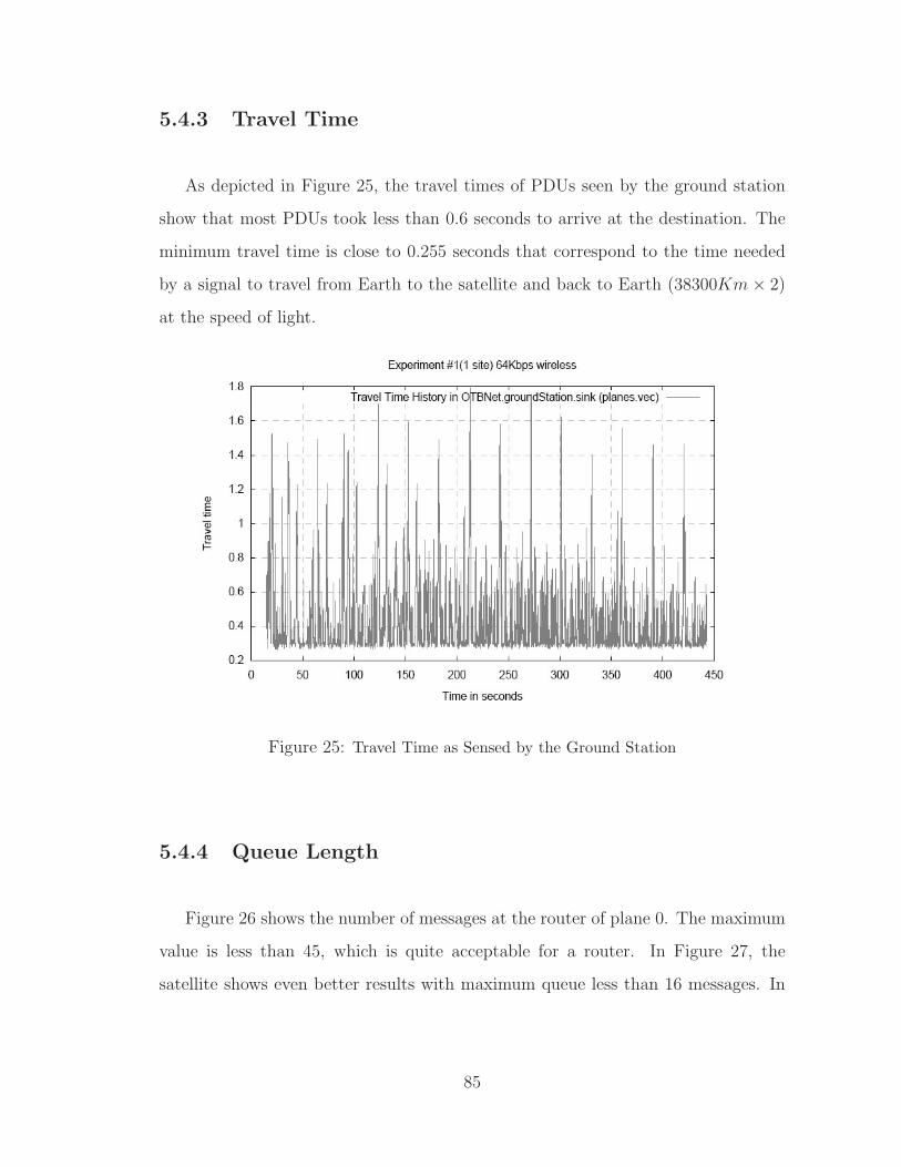
5.4.3 Travel Time
As depicted in Figure 25, the travel times of PDUs seen by the ground station
show that most PDUs took less than 0.6 seconds to arrive at the destination. The
minimum travel time is close to 0.255 seconds that correspond to the time needed
by a signal to travel from Earth to the satellite and back to Earth (38300Km × 2)
at the speed of light.
Figure 25: Travel Time as Sensed by the Ground Station
5.4.4 Queue Length
Figure 26 shows the number of messages at the router of plane 0. The maximum
value is less than 45, which is quite acceptable for a router. In Figure 27, the
satellite shows even better results with maximum queue less than 16 messages. In
85

both instances, the queue usage has similar characteristics throughout the simulation
time, showing peaks of all sizes evenly distributed along the time.
Figure 26: Messages in Router 0 (plane 0)
5.4.5 Collisions
No collisions were detected. This is understandable due to the fact that only one
site is transmitting.
5.4.6 Conclusions of Simulation 1
This first simulation was based on a simple vignette. The main purpose was
really to test the simulator itself. All the wireless links were set to a bandwidth of
64 Kbps. The results are congruent with the expected values for such a simulation.
86
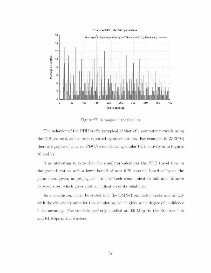
Figure 27: Messages in the Satellite
The behavior of the PDU traffic is typical of that of a computer network using
the DIS protocol, as has been reported by other authors. For example, in [MZP94]
there are graphs of time vs. PDU/second showing similar PDU activity as in Figures
26 and 27.
It is interesting to note that the simulator calculates the PDU travel time to
the ground station with a lower bound of near 0.25 seconds, based solely on the
parameters given, as propagation time of each communication link and distance
between sites, which gives another indication of its reliability.
As a conclusion, it can be stated that the OMNeT simulator works accordingly
with the expected results for this simulation, which gives some degree of confidence
in its accuracy. The traffic is perfectly handled at 100 Mbps in the Ethernet link
and 64 Kbps in the wireless.
87
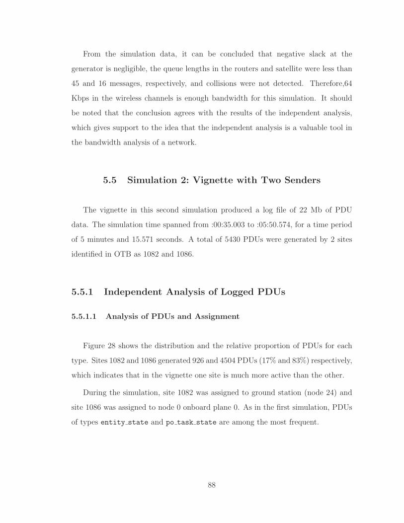
From the simulation data, it can be concluded that negative slack at the
generator is negligible, the queue lengths in the routers and satellite were less than
45 and 16 messages, respectively, and collisions were not detected. Therefore,64
Kbps in the wireless channels is enough bandwidth for this simulation. It should
be noted that the conclusion agrees with the results of the independent analysis,
which gives support to the idea that the independent analysis is a valuable tool in
the bandwidth analysis of a network.
5.5 Simulation 2: Vignette with Two Senders
The vignette in this second simulation produced a log file of 22 Mb of PDU
data. The simulation time spanned from :00:35.003 to :05:50.574, for a time period
of 5 minutes and 15.571 seconds. A total of 5430 PDUs were generated by 2 sites
identified in OTB as 1082 and 1086.
5.5.1 Independent Analysis of Logged PDUs
5.5.1.1 Analysis of PDUs and Assignment
Figure 28 shows the distribution and the relative proportion of PDUs for each
type. Sites 1082 and 1086 generated 926 and 4504 PDUs (17% and 83%) respectively,
which indicates that in the vignette one site is much more active than the other.
During the simulation, site 1082 was assigned to ground station (node 24) and
site 1086 was assigned to node 0 onboard plane 0. As in the first simulation, PDUs
of types entity state and po task state are among the most frequent.
88
<dis204 stop_freeze PDU>: 3<dis204 start_resume PDU>: 3<dis204 po_delete_objects PDU>: 7<dis204 acknowledge PDU>: 12<dis204 po_link PDU>: 12<dis204 aggregate_state PDU>: 18<dis204 fire PDU>: 24<dis204 detonation PDU>: 24<dis204 po_simulator_present PDU>: 26<dis204 signal PDU>: 27<dis204 po_parametric_input_holder PDU>:40<dis204 po_objects_present PDU>: 52<dis204 po_overlay PDU>: 64<dis204 po_line PDU>: 65<dis204 po_fire_parameters PDU>: 65<dis204 po_point PDU>: 80<dis204 po_task_frame PDU>: 85<dis204 po_parametric_input PDU>: 165<dis204 po_unit PDU>: 186<dis204 emissions PDU>: 204<dis204 transmitter PDU>: 547<dis204 po_variable PDU>: 760<dis204 po_task PDU>: 835<dis204 entity_state PDU>: 1021<dis204 po_task_state PDU>: 1105Total PDUs = 5430
Figure 28: PDU Type Distribution Generated in Simulation 2
5.5.1.2 Minimum Bandwidth Requirements
Figure 29 shows a high bandwidth spike near the second 95. The reason is that
lots of PDUs are scheduled to be sent at times close to second 95. A close look
at the data shows that during the time interval [92.463000, 94.484000], 310 PDUs
totaling 957 K bits are being scheduled. This volume of data requires approximately
474 Kbps to be sent on time. After the second 100, the remaining PDUs can be
handled at 64 Kbps, as Figure 29 indicates. Because the bandwidth is considered
constant in the actual links, 64 Kpbs will be insufficient to fulfill the needs of this
second vignette.
5.5.2 Slack Time
Figure sim2:slack1 shows the slack time as seen by computer node 0 (line labeled
1) and the ground station (line labeled 2), setting the wireless bandwidth to 64 Kbps.
89
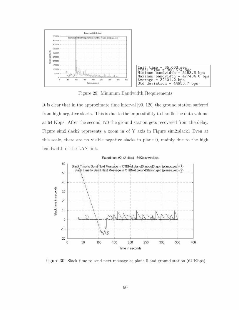
Init time = 35.003 sec.Final time = 350.574 sec.Minimum bandwidth = 5153.6 bpsMaximum bandwidth = 477404.0 bpsAverage = 32401.2 bpsStd deviation = 44953.7 bps
Figure 29: Minimum Bandwidth Requirements
It is clear that in the approximate time interval [90, 120] the ground station suffered
from high negative slacks. This is due to the impossibility to handle the data volume
at 64 Kbps. After the second 120 the ground station gets recovered from the delay.
Figure sim2:slack2 represents a zoom in of Y axis in Figure sim2:slack1 Even at
this scale, there are no visible negative slacks in plane 0, mainly due to the high
bandwidth of the LAN link.
Figure 30: Slack time to send next message at plane 0 and ground station (64 Kbps)
90
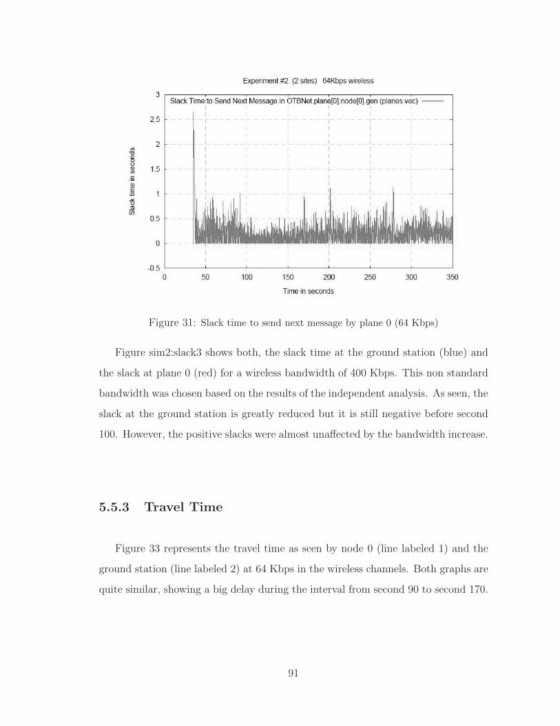
Figure 31: Slack time to send next message by plane 0 (64 Kbps)
Figure sim2:slack3 shows both, the slack time at the ground station (blue) and
the slack at plane 0 (red) for a wireless bandwidth of 400 Kbps. This non standard
bandwidth was chosen based on the results of the independent analysis. As seen, the
slack at the ground station is greatly reduced but it is still negative before second
100. However, the positive slacks were almost unaffected by the bandwidth increase.
5.5.3 Travel Time
Figure 33 represents the travel time as seen by node 0 (line labeled 1) and the
ground station (line labeled 2) at 64 Kbps in the wireless channels. Both graphs are
quite similar, showing a big delay during the interval from second 90 to second 170.
91

Figure 32: Slack time to send next message by plane 0 and ground station (400 Kbps)
Figure 33: Travel times at plane 0 and ground station (64 Kbps)
92
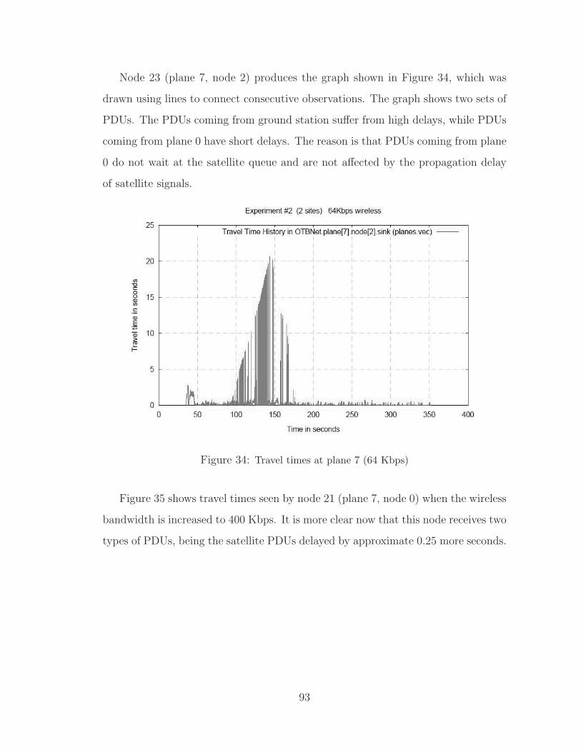
Node 23 (plane 7, node 2) produces the graph shown in Figure 34, which was
drawn using lines to connect consecutive observations. The graph shows two sets of
PDUs. The PDUs coming from ground station suffer from high delays, while PDUs
coming from plane 0 have short delays. The reason is that PDUs coming from plane
0 do not wait at the satellite queue and are not affected by the propagation delay
of satellite signals.
Figure 34: Travel times at plane 7 (64 Kbps)
Figure 35 shows travel times seen by node 21 (plane 7, node 0) when the wireless
bandwidth is increased to 400 Kbps. It is more clear now that this node receives two
types of PDUs, being the satellite PDUs delayed by approximate 0.25 more seconds.
93
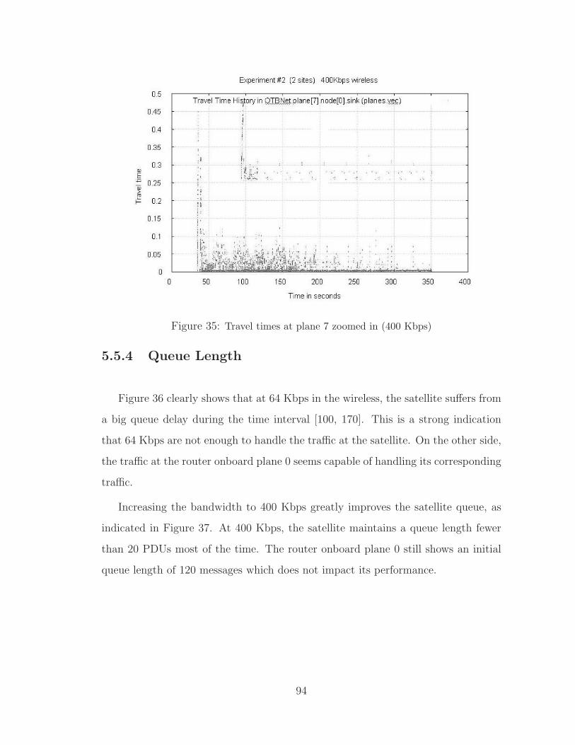
Figure 35: Travel times at plane 7 zoomed in (400 Kbps)
5.5.4 Queue Length
Figure 36 clearly shows that at 64 Kbps in the wireless, the satellite suffers from
a big queue delay during the time interval [100, 170]. This is a strong indication
that 64 Kbps are not enough to handle the traffic at the satellite. On the other side,
the traffic at the router onboard plane 0 seems capable of handling its corresponding
traffic.
Increasing the bandwidth to 400 Kbps greatly improves the satellite queue, as
indicated in Figure 37. At 400 Kbps, the satellite maintains a queue length fewer
than 20 PDUs most of the time. The router onboard plane 0 still shows an initial
queue length of 120 messages which does not impact its performance.
94
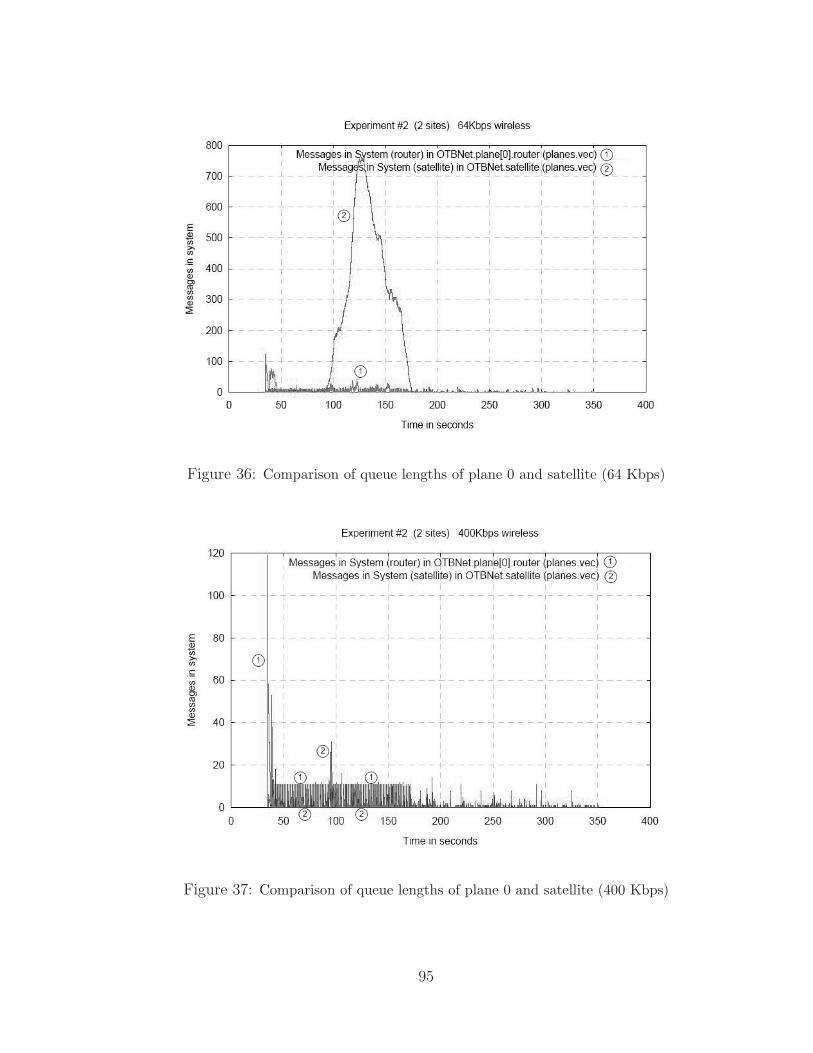
Figure 36: Comparison of queue lengths of plane 0 and satellite (64 Kbps)
Figure 37: Comparison of queue lengths of plane 0 and satellite (400 Kbps)
95
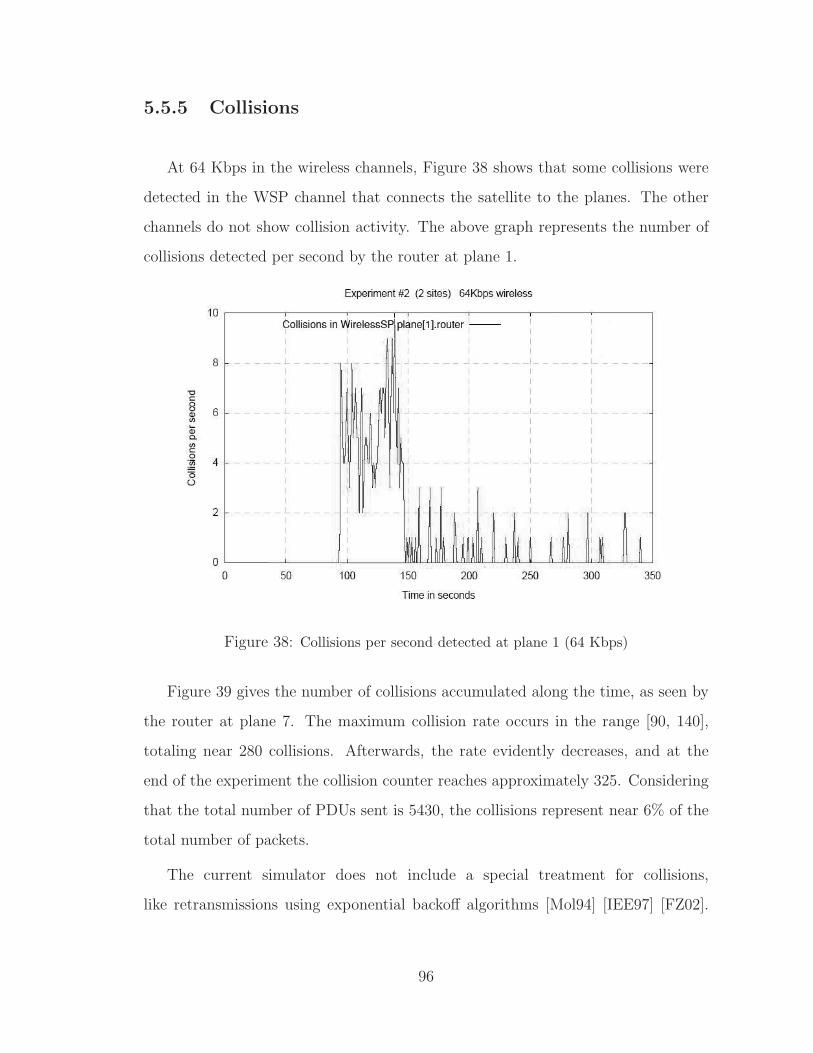
5.5.5 Collisions
At 64 Kbps in the wireless channels, Figure 38 shows that some collisions were
detected in the WSP channel that connects the satellite to the planes. The other
channels do not show collision activity. The above graph represents the number of
collisions detected per second by the router at plane 1.
Figure 38: Collisions per second detected at plane 1 (64 Kbps)
Figure 39 gives the number of collisions accumulated along the time, as seen by
the router at plane 7. The maximum collision rate occurs in the range [90, 140],
totaling near 280 collisions. Afterwards, the rate evidently decreases, and at the
end of the experiment the collision counter reaches approximately 325. Considering
that the total number of PDUs sent is 5430, the collisions represent near 6% of the
total number of packets.
The current simulator does not include a special treatment for collisions,
like retransmissions using exponential backoff algorithms [Mol94] [IEE97] [FZ02].
96
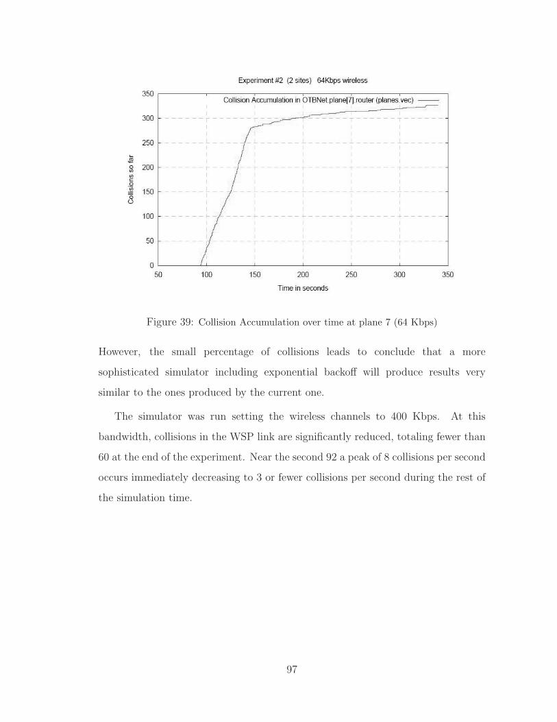
Figure 39: Collision Accumulation over time at plane 7 (64 Kbps)
However, the small percentage of collisions leads to conclude that a more
sophisticated simulator including exponential backoff will produce results very
similar to the ones produced by the current one.
The simulator was run setting the wireless channels to 400 Kbps. At this
bandwidth, collisions in the WSP link are significantly reduced, totaling fewer than
60 at the end of the experiment. Near the second 92 a peak of 8 collisions per second
occurs immediately decreasing to 3 or fewer collisions per second during the rest of
the simulation time.
97
5.5.6 Conclusions of Simulation 2
As indicated at the beginning of the chapter, the two first simulations were used
mainly to test the logic and general behavior of the OMNeT simulator, as well as
for taking a closer look at the PDUs, their distribution and initial statistics.
As predicted in the independent analysis, 64 Kbps in the wireless channels is
insufficient bandwidth to handle traffic near the interval [90, 175] seconds. After
second 175 the traffic becomes less intense and can be handled. Based on the
independent analysis, increasing the bandwidth to 400 Kbps in wireless channels
produce much better results, with travel times less than 0.5 seconds for all packets.
Collisions were detected in the WSP link only, but at 400 Kbps, the total number is
less than 60. At 64 Kbps, the queue length was close to 750 PDUs in the satellite,
number that decreases under 30 PDUs at 400 Kbps. Assuming the worst case
length in the satellite queue, 750 PDUs of 1368 bytes each would require near 1 Mb
of memory, which does not impose a tight restriction.
5.6 Simulation 3: Vignette MR1 with Six Senders
Simulation 3, as well as the remaining ones, is based on the MR1 vignette
described in Appendix A. The log file for this simulation is 265 Mb long. The
simulation time spanned from :17:14.447 to :42:27.808, for a time period of 25
minutes and 13.361 seconds. A total of 60341 PDUs were generated by 6 sites
identified in OTB as 1519, 1526, 1529, 1532, 1533, and 1538. The simulation is not
using the bundling technique. Bundling simulations are covered in Chapter 6.
98
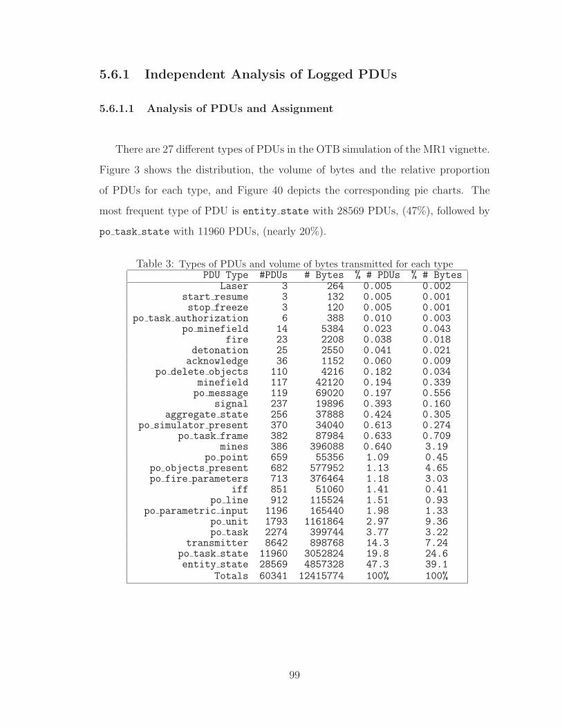
5.6.1 Independent Analysis of Logged PDUs
5.6.1.1 Analysis of PDUs and Assignment
There are 27 different types of PDUs in the OTB simulation of the MR1 vignette.
Figure 3 shows the distribution, the volume of bytes and the relative proportion
of PDUs for each type, and Figure 40 depicts the corresponding pie charts. The
most frequent type of PDU is entity state with 28569 PDUs, (47%), followed by
po task state with 11960 PDUs, (nearly 20%).
Table 3: Types of PDUs and volume of bytes transmitted for each typePDU Type #PDUs # Bytes % # PDUs % # Bytes
Laser 3 264 0.005 0.002start resume 3 132 0.005 0.001stop freeze 3 120 0.005 0.001
po task authorization 6 388 0.010 0.003po minefield 14 5384 0.023 0.043
fire 23 2208 0.038 0.018detonation 25 2550 0.041 0.021
acknowledge 36 1152 0.060 0.009po delete objects 110 4216 0.182 0.034
minefield 117 42120 0.194 0.339po message 119 69020 0.197 0.556
signal 237 19896 0.393 0.160aggregate state 256 37888 0.424 0.305
po simulator present 370 34040 0.613 0.274po task frame 382 87984 0.633 0.709
mines 386 396088 0.640 3.19po point 659 55356 1.09 0.45
po objects present 682 577952 1.13 4.65po fire parameters 713 376464 1.18 3.03
iff 851 51060 1.41 0.41po line 912 115524 1.51 0.93
po parametric input 1196 165440 1.98 1.33po unit 1793 1161864 2.97 9.36po task 2274 399744 3.77 3.22
transmitter 8642 898768 14.3 7.24po task state 11960 3052824 19.8 24.6entity state 28569 4857328 47.3 39.1
Totals 60341 12415774 100% 100%
99
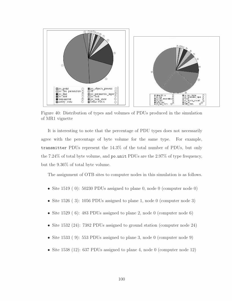
Figure 40: Distribution of types and volumes of PDUs produced in the simulationof MR1 vignette
It is interesting to note that the percentage of PDU types does not necessarily
agree with the percentage of byte volume for the same type. For example,
transmitter PDUs represent the 14.3% of the total number of PDUs, but only
the 7.24% of total byte volume, and po unit PDUs are the 2.97% of type frequency,
but the 9.36% of total byte volume.
The assignment of OTB sites to computer nodes in this simulation is as follows.
• Site 1519 ( 0): 50230 PDUs assigned to plane 0, node 0 (computer node 0)
• Site 1526 ( 3): 1056 PDUs assigned to plane 1, node 0 (computer node 3)
• Site 1529 ( 6): 483 PDUs assigned to plane 2, node 0 (computer node 6)
• Site 1532 (24): 7382 PDUs assigned to ground station (computer node 24)
• Site 1533 ( 9): 553 PDUs assigned to plane 3, node 0 (computer node 9)
• Site 1538 (12): 637 PDUs assigned to plane 4, node 0 (computer node 12)
100
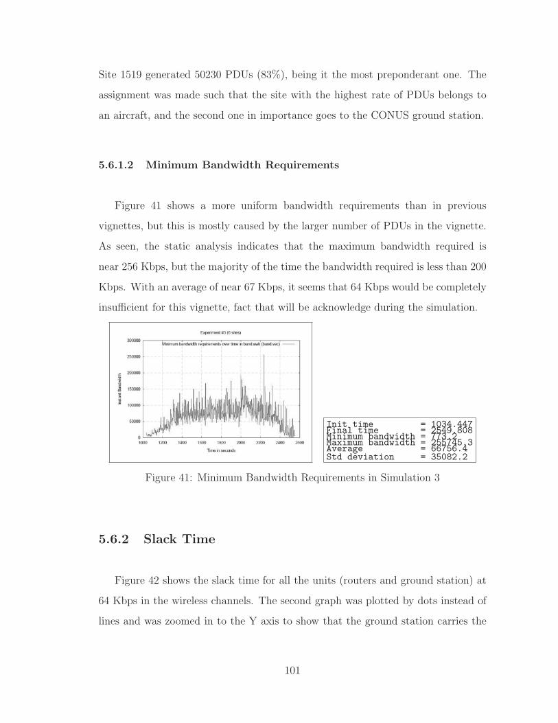
Site 1519 generated 50230 PDUs (83%), being it the most preponderant one. The
assignment was made such that the site with the highest rate of PDUs belongs to
an aircraft, and the second one in importance goes to the CONUS ground station.
5.6.1.2 Minimum Bandwidth Requirements
Figure 41 shows a more uniform bandwidth requirements than in previous
vignettes, but this is mostly caused by the larger number of PDUs in the vignette.
As seen, the static analysis indicates that the maximum bandwidth required is
near 256 Kbps, but the majority of the time the bandwidth required is less than 200
Kbps. With an average of near 67 Kbps, it seems that 64 Kbps would be completely
insufficient for this vignette, fact that will be acknowledge during the simulation.
Init time = 1034.447Final time = 2549.808Minimum bandwidth = 773.2Maximum bandwidth = 255745.3Average = 66756.4Std deviation = 35082.2
Figure 41: Minimum Bandwidth Requirements in Simulation 3
5.6.2 Slack Time
Figure 42 shows the slack time for all the units (routers and ground station) at
64 Kbps in the wireless channels. The second graph was plotted by dots instead of
lines and was zoomed in to the Y axis to show that the ground station carries the
101
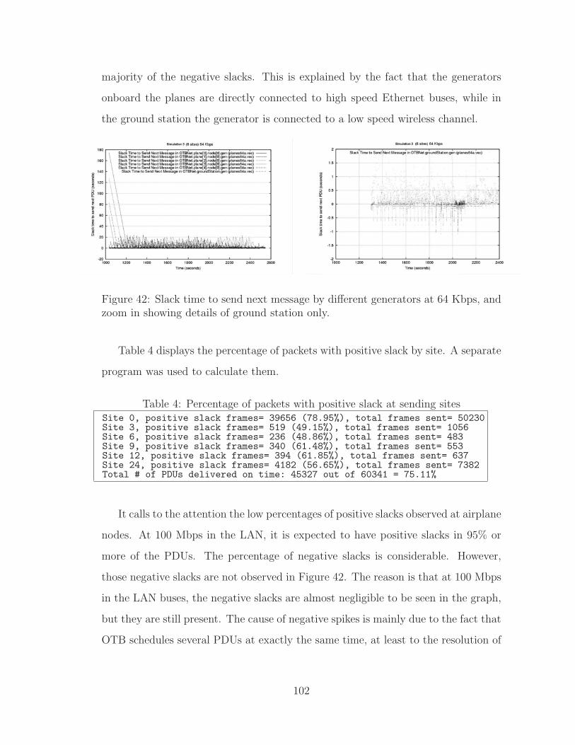
majority of the negative slacks. This is explained by the fact that the generators
onboard the planes are directly connected to high speed Ethernet buses, while in
the ground station the generator is connected to a low speed wireless channel.
Figure 42: Slack time to send next message by different generators at 64 Kbps, andzoom in showing details of ground station only.
Table 4 displays the percentage of packets with positive slack by site. A separate
program was used to calculate them.
Table 4: Percentage of packets with positive slack at sending sitesSite 0, positive slack frames= 39656 (78.95%), total frames sent= 50230Site 3, positive slack frames= 519 (49.15%), total frames sent= 1056Site 6, positive slack frames= 236 (48.86%), total frames sent= 483Site 9, positive slack frames= 340 (61.48%), total frames sent= 553Site 12, positive slack frames= 394 (61.85%), total frames sent= 637Site 24, positive slack frames= 4182 (56.65%), total frames sent= 7382Total # of PDUs delivered on time: 45327 out of 60341 = 75.11%
It calls to the attention the low percentages of positive slacks observed at airplane
nodes. At 100 Mbps in the LAN, it is expected to have positive slacks in 95% or
more of the PDUs. The percentage of negative slacks is considerable. However,
those negative slacks are not observed in Figure 42. The reason is that at 100 Mbps
in the LAN buses, the negative slacks are almost negligible to be seen in the graph,
but they are still present. The cause of negative spikes is mainly due to the fact that
OTB schedules several PDUs at exactly the same time, at least to the resolution of
102
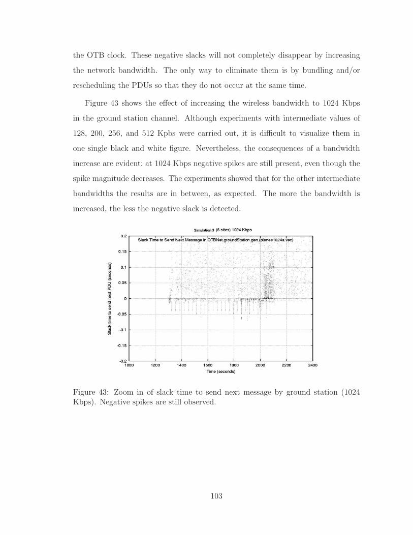
the OTB clock. These negative slacks will not completely disappear by increasing
the network bandwidth. The only way to eliminate them is by bundling and/or
rescheduling the PDUs so that they do not occur at the same time.
Figure 43 shows the effect of increasing the wireless bandwidth to 1024 Kbps
in the ground station channel. Although experiments with intermediate values of
128, 200, 256, and 512 Kpbs were carried out, it is difficult to visualize them in
one single black and white figure. Nevertheless, the consequences of a bandwidth
increase are evident: at 1024 Kbps negative spikes are still present, even though the
spike magnitude decreases. The experiments showed that for the other intermediate
bandwidths the results are in between, as expected. The more the bandwidth is
increased, the less the negative slack is detected.
Figure 43: Zoom in of slack time to send next message by ground station (1024Kbps). Negative spikes are still observed.
103
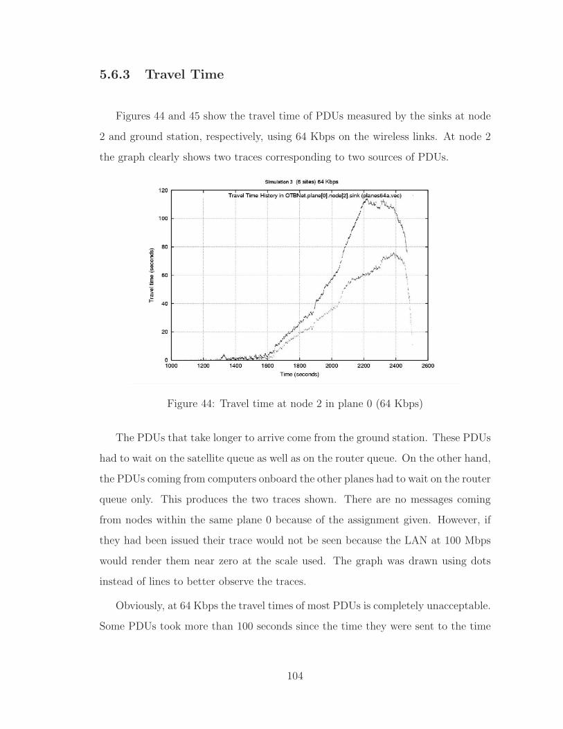
5.6.3 Travel Time
Figures 44 and 45 show the travel time of PDUs measured by the sinks at node
2 and ground station, respectively, using 64 Kbps on the wireless links. At node 2
the graph clearly shows two traces corresponding to two sources of PDUs.
Figure 44: Travel time at node 2 in plane 0 (64 Kbps)
The PDUs that take longer to arrive come from the ground station. These PDUs
had to wait on the satellite queue as well as on the router queue. On the other hand,
the PDUs coming from computers onboard the other planes had to wait on the router
queue only. This produces the two traces shown. There are no messages coming
from nodes within the same plane 0 because of the assignment given. However, if
they had been issued their trace would not be seen because the LAN at 100 Mbps
would render them near zero at the scale used. The graph was drawn using dots
instead of lines to better observe the traces.
Obviously, at 64 Kbps the travel times of most PDUs is completely unacceptable.
Some PDUs took more than 100 seconds since the time they were sent to the time
104

Figure 45: Travel time at ground station (64 Kbps)
they arrived. The ground station presents a similar behavior due to the long queue
times at the satellite.
Figure 46 shows travel times measured at the ground station for bandwidths of
64 and 256 Kbps. The graph was zoomed in to the Y axis to show the details in
the neighborhood of 0 to 2 seconds. The spots at the left side having travel times
over 1 second correspond to 64 Kpbs, while the other spots that almost do not
reach the 1 second limit correspond to 256 Kpbs. It is worth noting the enormous
difference between these two bandwidths. At 256 Kbps in the wireless channels,
the travel times to the ground station are less than 1 second in the majority of
cases. Considering that the minimum travel time is about 0.25 seconds, latencies
less than 1 second can be acceptable, especially if OTB could deliver the PDUs in
a not-so-bursting mode.
At 256 Kbps Figure 46 shows many discrete positive peaks separated at regular
intervals that could be diminish by a better scheduling policy. The positive travel
105
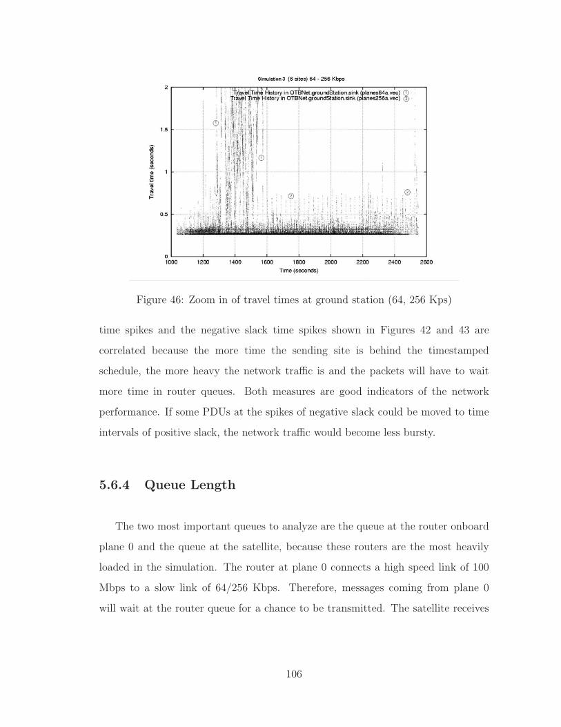
Figure 46: Zoom in of travel times at ground station (64, 256 Kps)
time spikes and the negative slack time spikes shown in Figures 42 and 43 are
correlated because the more time the sending site is behind the timestamped
schedule, the more heavy the network traffic is and the packets will have to wait
more time in router queues. Both measures are good indicators of the network
performance. If some PDUs at the spikes of negative slack could be moved to time
intervals of positive slack, the network traffic would become less bursty.
5.6.4 Queue Length
The two most important queues to analyze are the queue at the router onboard
plane 0 and the queue at the satellite, because these routers are the most heavily
loaded in the simulation. The router at plane 0 connects a high speed link of 100
Mbps to a slow link of 64/256 Kbps. Therefore, messages coming from plane 0
will wait at the router queue for a chance to be transmitted. The satellite receives
106

and transmits all the messages at low speeds, which constitutes a bottleneck in the
system. The routers at other planes not heavily transmitting PDUs take packets
from a slow wireless channel and pass them to a fast Ethernet link, resulting in
almost no queue waiting time. Nevertheless, the queue at another router is shown
as a sample of the behavior of the other routers.
Figure 47 represents the number of messages in the router at node 0, using
64 Kbps in the wireless channels. The queue length becomes really unacceptable,
reaching more than 3000 messages during some periods.
Figure 47: Messages in system at plane 0 (64 Kbps)
On the contrary, Figure 48 shows that the router at plane 3 has a normal
queue with a maximum of 23 messages. The reason for the short queue is that
the corresponding node 9 transmits only 553 PDUs, which are easily handled by the
router.
Figure 49 shows that the queue at the satellite (64 Kbps) has an unacceptable
behavior with a peak of more than 2200 messages.
Figure 50 shows the effect on the queue length of the router onboard plane 0
when the bandwidth increases from 64 to 256 Kbps. As a result, the queue length
107
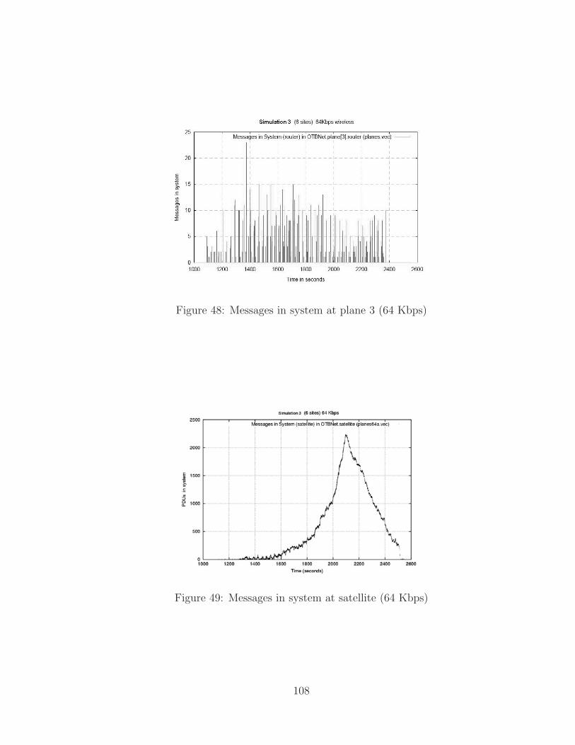
Figure 48: Messages in system at plane 3 (64 Kbps)
Figure 49: Messages in system at satellite (64 Kbps)
108

decreases to less than 50 messages in its highest peak. Therefore, the change of
speed greatly reduces the router queue.
Figure 50: Zoom in of messages in system at plane 0 (64 and 256 Kbps)
At the satellite, the change in the queue length is also noticeable, as shown in
Figure 51. At 256 Kbps, less than 25 messages are held in the satellite during the
highest peak.
5.6.5 Collisions
There are two factors that influence the way collisions are detected and analyzed
in the OMNeT simulator.
First, the simulator considers the transmission media as an ideal bus in the sense
that a wave does not become weaker by traveling long distances. As a result, two
waves coming form opposite directions can collide in the middle of the bus, but they
will continue their ways without being destroyed. Therefore, only a listener located
at the collision point can detect the collision. In other words, it is perfectly possible
for a collision to be detected at some point of the bus and not at others. Due to
109
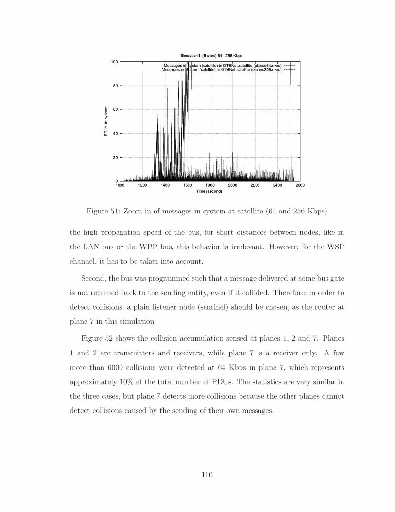
Figure 51: Zoom in of messages in system at satellite (64 and 256 Kbps)
the high propagation speed of the bus, for short distances between nodes, like in
the LAN bus or the WPP bus, this behavior is irrelevant. However, for the WSP
channel, it has to be taken into account.
Second, the bus was programmed such that a message delivered at some bus gate
is not returned back to the sending entity, even if it collided. Therefore, in order to
detect collisions, a plain listener node (sentinel) should be chosen, as the router at
plane 7 in this simulation.
Figure 52 shows the collision accumulation sensed at planes 1, 2 and 7. Planes
1 and 2 are transmitters and receivers, while plane 7 is a receiver only. A few
more than 6000 collisions were detected at 64 Kbps in plane 7, which represents
approximately 10% of the total number of PDUs. The statistics are very similar in
the three cases, but plane 7 detects more collisions because the other planes cannot
detect collisions caused by the sending of their own messages.
110
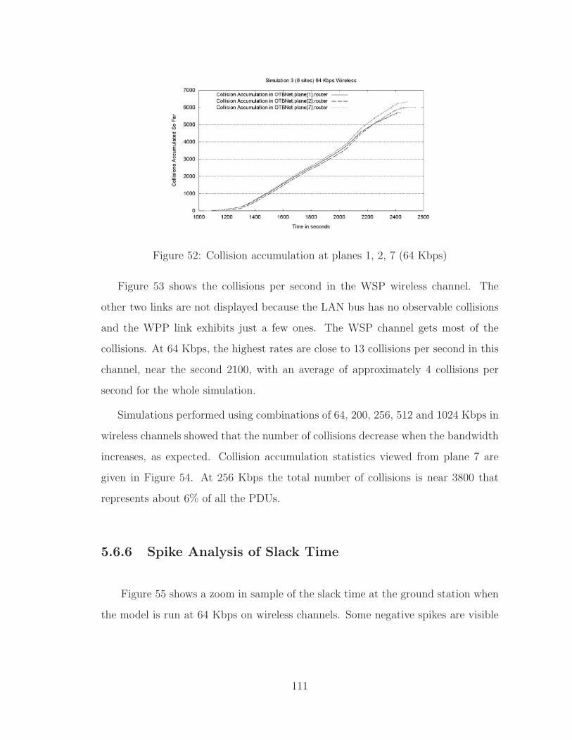
Figure 52: Collision accumulation at planes 1, 2, 7 (64 Kbps)
Figure 53 shows the collisions per second in the WSP wireless channel. The
other two links are not displayed because the LAN bus has no observable collisions
and the WPP link exhibits just a few ones. The WSP channel gets most of the
collisions. At 64 Kbps, the highest rates are close to 13 collisions per second in this
channel, near the second 2100, with an average of approximately 4 collisions per
second for the whole simulation.
Simulations performed using combinations of 64, 200, 256, 512 and 1024 Kbps in
wireless channels showed that the number of collisions decrease when the bandwidth
increases, as expected. Collision accumulation statistics viewed from plane 7 are
given in Figure 54. At 256 Kbps the total number of collisions is near 3800 that
represents about 6% of all the PDUs.
5.6.6 Spike Analysis of Slack Time
Figure 55 shows a zoom in sample of the slack time at the ground station when
the model is run at 64 Kbps on wireless channels. Some negative spikes are visible
111
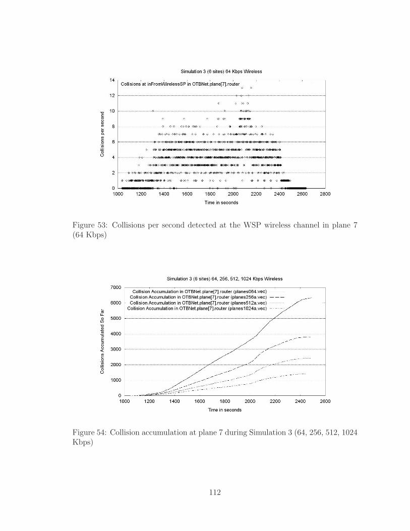
Figure 53: Collisions per second detected at the WSP wireless channel in plane 7(64 Kbps)
Figure 54: Collision accumulation at plane 7 during Simulation 3 (64, 256, 512, 1024Kbps)
112

at regular time intervals. Positive points indicate that the bandwidth is enough
to handle the PDUs in the neighborhood previous to the point. On the contrary,
negative spikes indicate a lack of bandwidth in the wireless channels. Those spikes
deserve more attention to understand and correct the problem. The OTB simulator
produces the negative spikes when multiple PDUs are scheduled at the same or
almost the same time. Identification of the PDUs responsible for the negative spikes
is the first step towards the study and possible modification of the OTB scheduling
policy.
Figure 55: Slack time at ground station showing negative spikes (64 Kbps)
Because the phenomenon seems to be cyclic, one initial approach to explain it
relays on the analysis of the different PDUs participating in the spike, correlating
them with actions occurring in the vignette at those times.
The sample includes the spikes captured in the time interval [1400, 1600] seconds.
This is a representative sample of spikes produced at the generators of PDUs. The
113
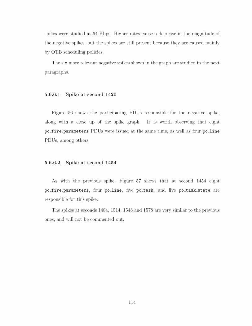
spikes were studied at 64 Kbps. Higher rates cause a decrease in the magnitude of
the negative spikes, but the spikes are still present because they are caused mainly
by OTB scheduling policies.
The six more relevant negative spikes shown in the graph are studied in the next
paragraphs.
5.6.6.1 Spike at second 1420
Figure 56 shows the participating PDUs responsible for the negative spike,
along with a close up of the spike graph. It is worth observing that eight
po fire parameters PDUs were issued at the same time, as well as four po line
PDUs, among others.
5.6.6.2 Spike at second 1454
As with the previous spike, Figure 57 shows that at second 1454 eight
po fire parameters, four po line, five po task, and five po task state are
responsible for this spike.
The spikes at seconds 1484, 1514, 1548 and 1578 are very similar to the previous
ones, and will not be commented out.
114
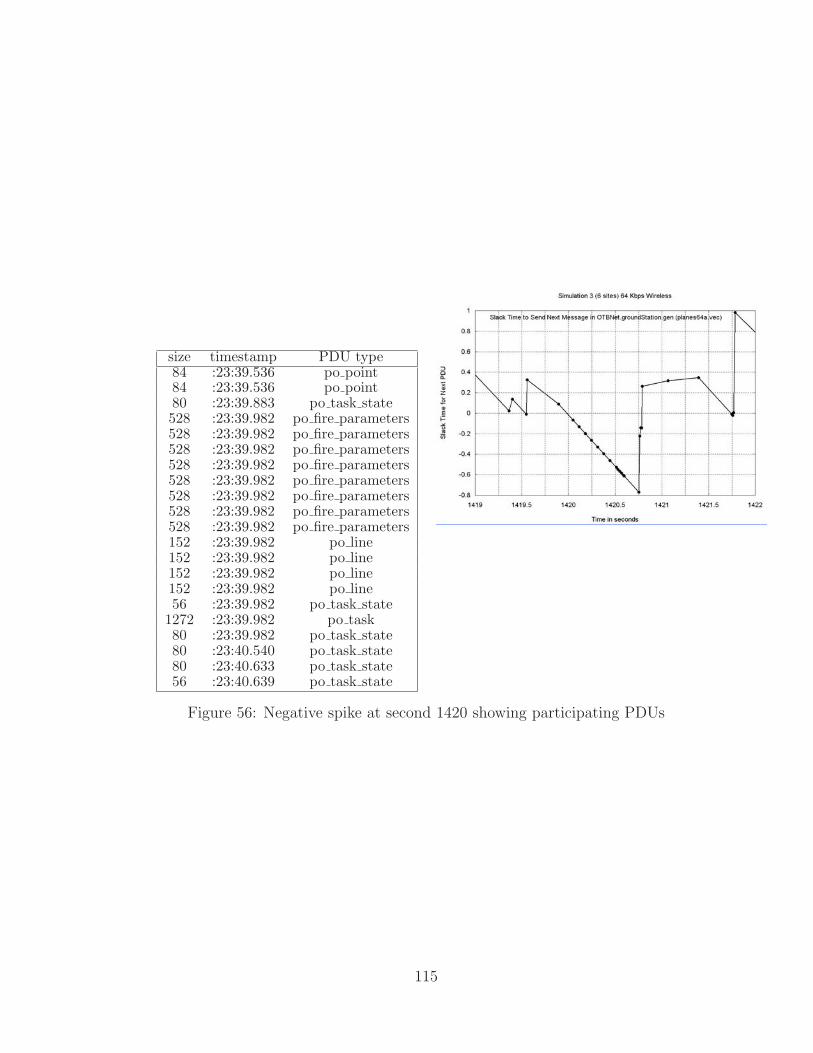
size timestamp PDU type84 :23:39.536 po point84 :23:39.536 po point80 :23:39.883 po task state528 :23:39.982 po fire parameters528 :23:39.982 po fire parameters528 :23:39.982 po fire parameters528 :23:39.982 po fire parameters528 :23:39.982 po fire parameters528 :23:39.982 po fire parameters528 :23:39.982 po fire parameters528 :23:39.982 po fire parameters152 :23:39.982 po line152 :23:39.982 po line152 :23:39.982 po line152 :23:39.982 po line56 :23:39.982 po task state
1272 :23:39.982 po task80 :23:39.982 po task state80 :23:40.540 po task state80 :23:40.633 po task state56 :23:40.639 po task state
Figure 56: Negative spike at second 1420 showing participating PDUs
115
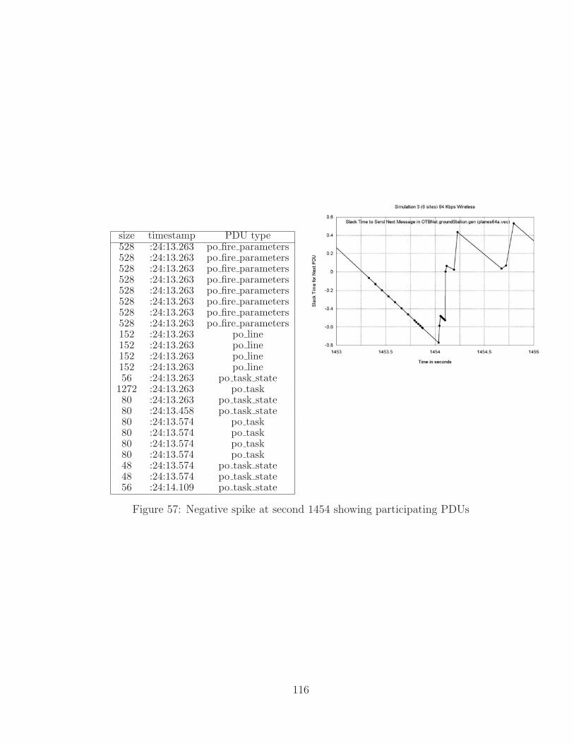
size timestamp PDU type528 :24:13.263 po fire parameters528 :24:13.263 po fire parameters528 :24:13.263 po fire parameters528 :24:13.263 po fire parameters528 :24:13.263 po fire parameters528 :24:13.263 po fire parameters528 :24:13.263 po fire parameters528 :24:13.263 po fire parameters152 :24:13.263 po line152 :24:13.263 po line152 :24:13.263 po line152 :24:13.263 po line56 :24:13.263 po task state
1272 :24:13.263 po task80 :24:13.263 po task state80 :24:13.458 po task state80 :24:13.574 po task80 :24:13.574 po task80 :24:13.574 po task80 :24:13.574 po task48 :24:13.574 po task state48 :24:13.574 po task state56 :24:14.109 po task state
Figure 57: Negative spike at second 1454 showing participating PDUs
116
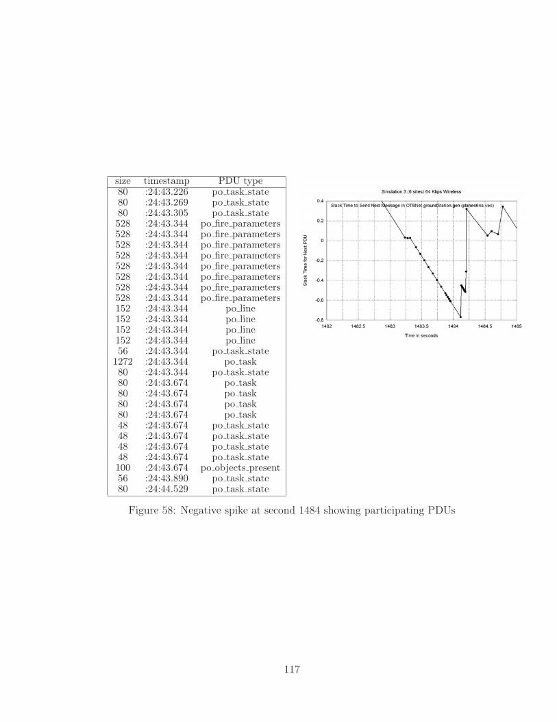
size timestamp PDU type80 :24:43.226 po task state80 :24:43.269 po task state80 :24:43.305 po task state528 :24:43.344 po fire parameters528 :24:43.344 po fire parameters528 :24:43.344 po fire parameters528 :24:43.344 po fire parameters528 :24:43.344 po fire parameters528 :24:43.344 po fire parameters528 :24:43.344 po fire parameters528 :24:43.344 po fire parameters152 :24:43.344 po line152 :24:43.344 po line152 :24:43.344 po line152 :24:43.344 po line56 :24:43.344 po task state
1272 :24:43.344 po task80 :24:43.344 po task state80 :24:43.674 po task80 :24:43.674 po task80 :24:43.674 po task80 :24:43.674 po task48 :24:43.674 po task state48 :24:43.674 po task state48 :24:43.674 po task state48 :24:43.674 po task state100 :24:43.674 po objects present56 :24:43.890 po task state80 :24:44.529 po task state
Figure 58: Negative spike at second 1484 showing participating PDUs
117
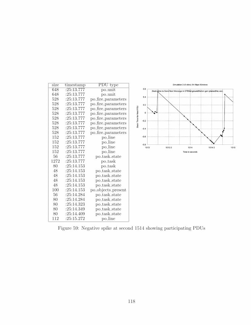
size timestamp PDU type648 :25:13.777 po unit648 :25:13.777 po unit528 :25:13.777 po fire parameters528 :25:13.777 po fire parameters528 :25:13.777 po fire parameters528 :25:13.777 po fire parameters528 :25:13.777 po fire parameters528 :25:13.777 po fire parameters528 :25:13.777 po fire parameters528 :25:13.777 po fire parameters152 :25:13.777 po line152 :25:13.777 po line152 :25:13.777 po line152 :25:13.777 po line56 :25:13.777 po task state
1272 :25:13.777 po task80 :25:14.153 po task48 :25:14.153 po task state48 :25:14.153 po task state48 :25:14.153 po task state48 :25:14.153 po task state100 :25:14.153 po objects present56 :25:14.284 po task state80 :25:14.284 po task state80 :25:14.323 po task state80 :25:14.349 po task state80 :25:14.409 po task state112 :25:15.272 po line
Figure 59: Negative spike at second 1514 showing participating PDUs
118
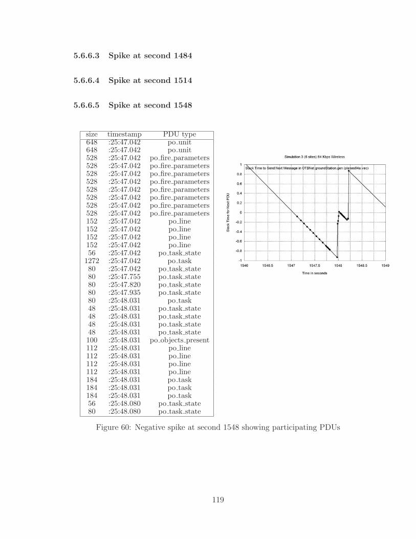
5.6.6.3 Spike at second 1484
5.6.6.4 Spike at second 1514
5.6.6.5 Spike at second 1548
size timestamp PDU type648 :25:47.042 po unit648 :25:47.042 po unit528 :25:47.042 po fire parameters528 :25:47.042 po fire parameters528 :25:47.042 po fire parameters528 :25:47.042 po fire parameters528 :25:47.042 po fire parameters528 :25:47.042 po fire parameters528 :25:47.042 po fire parameters528 :25:47.042 po fire parameters152 :25:47.042 po line152 :25:47.042 po line152 :25:47.042 po line152 :25:47.042 po line56 :25:47.042 po task state
1272 :25:47.042 po task80 :25:47.042 po task state80 :25:47.755 po task state80 :25:47.820 po task state80 :25:47.935 po task state80 :25:48.031 po task48 :25:48.031 po task state48 :25:48.031 po task state48 :25:48.031 po task state48 :25:48.031 po task state100 :25:48.031 po objects present112 :25:48.031 po line112 :25:48.031 po line112 :25:48.031 po line112 :25:48.031 po line184 :25:48.031 po task184 :25:48.031 po task184 :25:48.031 po task56 :25:48.080 po task state80 :25:48.080 po task state
Figure 60: Negative spike at second 1548 showing participating PDUs
119
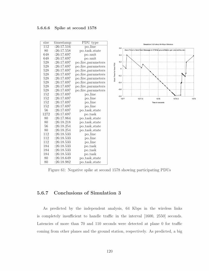
5.6.6.6 Spike at second 1578
size timestamp PDU type112 :26:17.516 po line80 :26:17.558 po task state648 :26:17.697 po unit648 :26:17.697 po unit528 :26:17.697 po fire parameters528 :26:17.697 po fire parameters528 :26:17.697 po fire parameters528 :26:17.697 po fire parameters528 :26:17.697 po fire parameters528 :26:17.697 po fire parameters528 :26:17.697 po fire parameters528 :26:17.697 po fire parameters152 :26:17.697 po line152 :26:17.697 po line152 :26:17.697 po line152 :26:17.697 po line56 :26:17.697 po task state
1272 :26:17.697 po task80 :26:17.864 po task state80 :26:18.218 po task state56 :26:18.254 po task state80 :26:18.254 po task state112 :26:18.533 po line112 :26:18.533 po line112 :26:18.533 po line184 :26:18.533 po task184 :26:18.533 po task184 :26:18.533 po task80 :26:18.649 po task state80 :26:18.982 po task state
Figure 61: Negative spike at second 1578 showing participating PDUs
5.6.7 Conclusions of Simulation 3
As predicted by the independent analysis, 64 Kbps in the wireless links
is completely insufficient to handle traffic in the interval [1600, 2550] seconds.
Latencies of more than 70 and 110 seconds were detected at plane 0 for traffic
coming from other planes and the ground station, respectively. As predicted, a big
120

improvement was achieved starting at 200 Kbps. Latencies less than 1 second were
almost always the rule for messages received at the ground station. At the router in
plane 0 and at the satellite, the queue lengths changed from 3400 and 2200 (max)
to less than 50 and less than 25 (max), respectively, just by changing the bandwidth
from 64 Kbps to 256 Kbps. Relatively few collisions were detected, which are not
enough to significantly change the results or conclusions. A summary of the total
number of collisions is given in Table 5.
Table 5: Total, relative percentage and average number of collisions per second inSimulation 3
Bandwidth Collisions Percentage Frequency
64 Kbps 6320 coll. 10.5% 4.2 coll/sec
200 Kbps 4434 coll. 7.3% 2.9 coll/sec
256 Kbps 3804 coll. 6.3% 2.5 coll/sec
512 Kbps 2421 coll. 4.0% 1.6 coll/sec
1024 Kbps 1416 coll. 2.3% 0.9 coll/sec
The negative spikes in slack time studied in Simulation 3 are very similar,
including three main types of PDUs: po fire parameters, po line and
po task state PDUs. In all cases, sequences of these PDUs were scheduled exactly
at the same time, causing the spike. It seems that the main sequence of PDUs in a
negative spike is of type po fire parameters, perhaps because the entity (ground
station) is firing against some enemy at regular time intervals.
5.7 Simulation 4: Vignette MR1 Revisited
Given that site 1519 assigned to node 0 in plane 0 for Simulation 3 generates
83% of all the PDUs, it seemed interesting to assign it to the CONUS ground
station connected to the satellite via a wireless channel. The idea was suggested
121
by PO STRI personnel during an update presentation. The results obtained
were certainly interesting, and leaded to the developing of the bundling algorithm
described in Section 3.4.2.
5.7.1 Independent Analysis of Logged PDUs andAssignment
This simulation makes use of the same data set as in Simulation 3, and so the
types of PDUs, data volumes and percentages remain the same. The only difference
is that the assignment of sites 1519 and 1532 corresponding to computer 0 and
ground station was swapped. Therefore, the assignment of sites to computers in
this experiment is as follows.
Site 1532 ( 0): 7382 PDUs assigned to plane 0, node 0
Site 1526 ( 3): 1056 PDUs assigned to plane 1, node 0
Site 1529 ( 6): 483 PDUs assigned to plane 2, node 0
Site 1533 ( 9): 553 PDUs assigned to plane 3, node 0
Site 1538 (12): 637 PDUs assigned to plane 4, node 0
Site 1519 (24): 50230 PDUs assigned to ground station
The minimum bandwidth requirements are the same as in Simulation 3 and can
be found in Figure 41.
122
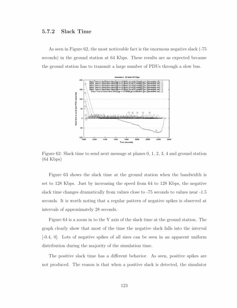
5.7.2 Slack Time
As seen in Figure 62, the most noticeable fact is the enormous negative slack (-75
seconds) in the ground station at 64 Kbps. These results are as expected because
the ground station has to transmit a large number of PDUs through a slow bus.
Figure 62: Slack time to send next message at planes 0, 1, 2, 3, 4 and ground station(64 Kbps)
Figure 63 shows the slack time at the ground station when the bandwidth is
set to 128 Kbps. Just by increasing the speed from 64 to 128 Kbps, the negative
slack time changes dramatically from values close to -75 seconds to values near -1.5
seconds. It is worth noting that a regular pattern of negative spikes is observed at
intervals of approximately 28 seconds.
Figure 64 is a zoom in to the Y axis of the slack time at the ground station. The
graph clearly show that most of the time the negative slack falls into the interval
[-0.4, 0]. Lots of negative spikes of all sizes can be seen in an apparent uniform
distribution during the majority of the simulation time.
The positive slack time has a different behavior. As seen, positive spikes are
not produced. The reason is that when a positive slack is detected, the simulator
123
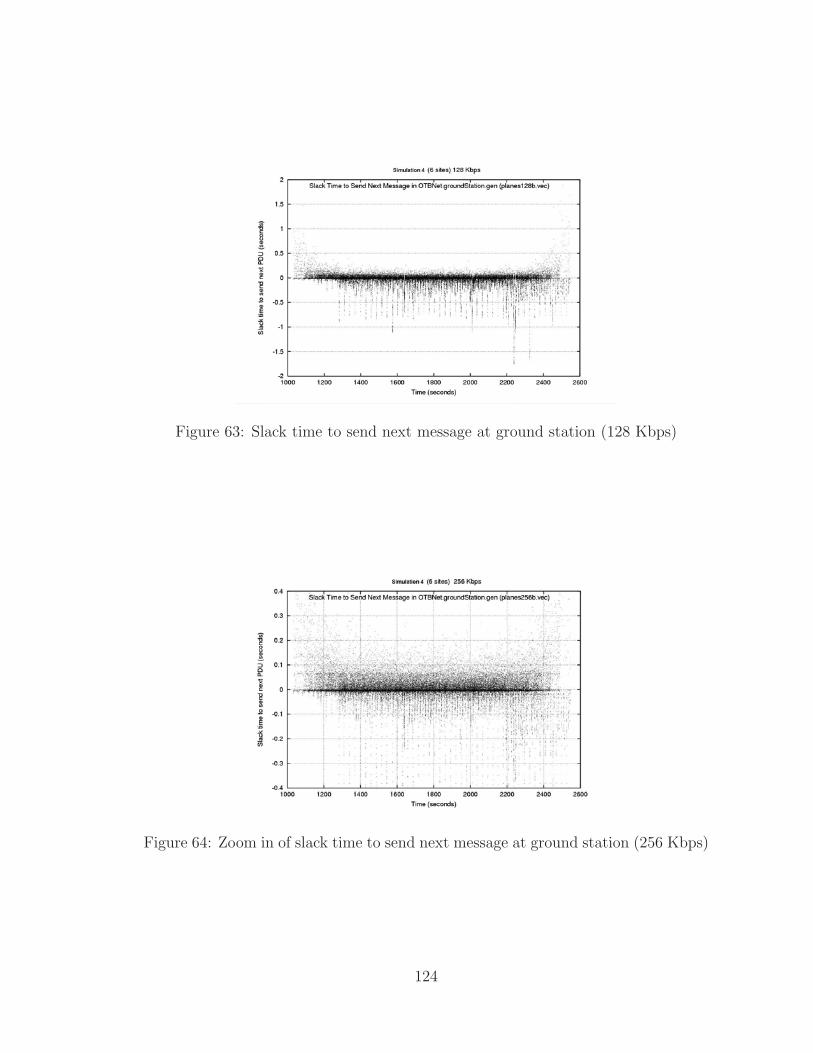
Figure 63: Slack time to send next message at ground station (128 Kbps)
Figure 64: Zoom in of slack time to send next message at ground station (256 Kbps)
124
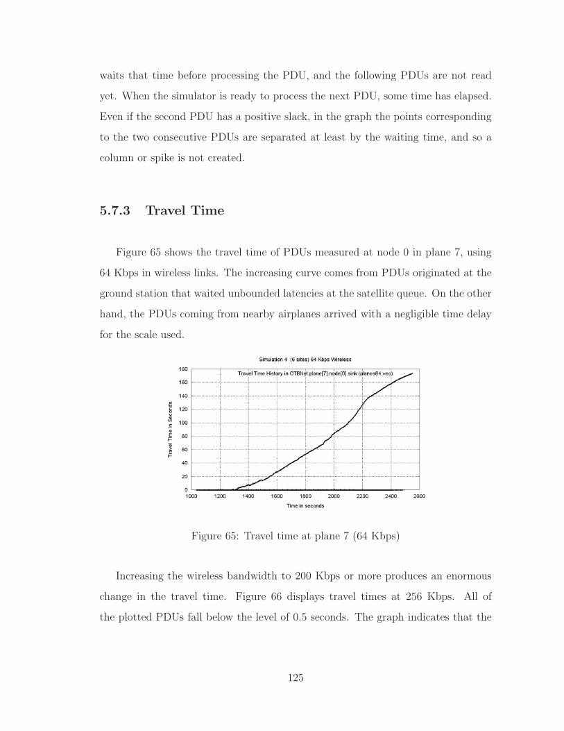
waits that time before processing the PDU, and the following PDUs are not read
yet. When the simulator is ready to process the next PDU, some time has elapsed.
Even if the second PDU has a positive slack, in the graph the points corresponding
to the two consecutive PDUs are separated at least by the waiting time, and so a
column or spike is not created.
5.7.3 Travel Time
Figure 65 shows the travel time of PDUs measured at node 0 in plane 7, using
64 Kbps in wireless links. The increasing curve comes from PDUs originated at the
ground station that waited unbounded latencies at the satellite queue. On the other
hand, the PDUs coming from nearby airplanes arrived with a negligible time delay
for the scale used.
Figure 65: Travel time at plane 7 (64 Kbps)
Increasing the wireless bandwidth to 200 Kbps or more produces an enormous
change in the travel time. Figure 66 displays travel times at 256 Kbps. All of
the plotted PDUs fall below the level of 0.5 seconds. The graph indicates that the
125
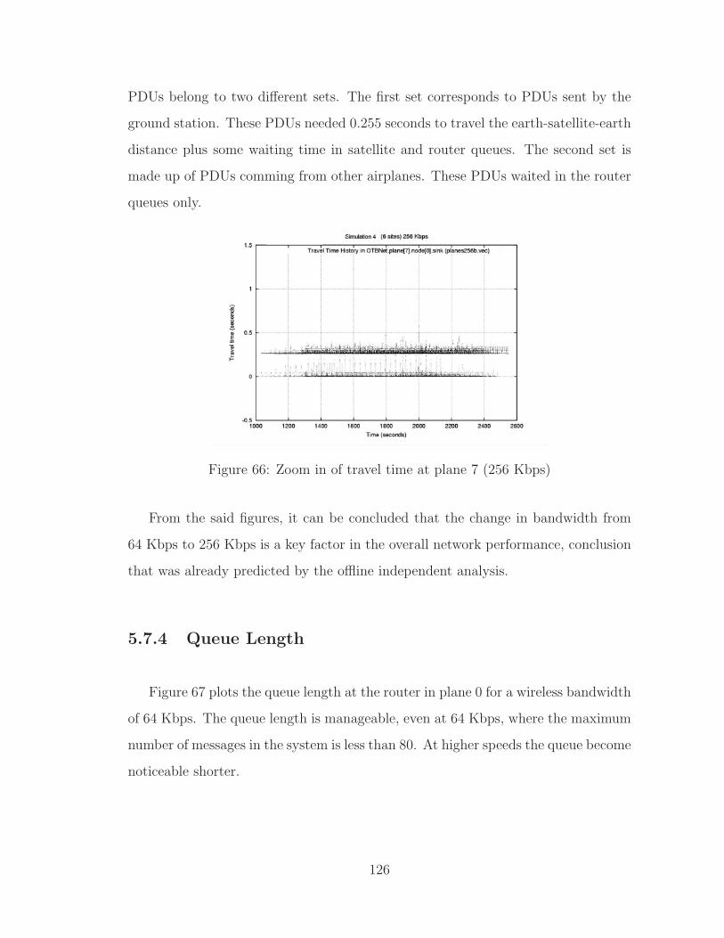
PDUs belong to two different sets. The first set corresponds to PDUs sent by the
ground station. These PDUs needed 0.255 seconds to travel the earth-satellite-earth
distance plus some waiting time in satellite and router queues. The second set is
made up of PDUs comming from other airplanes. These PDUs waited in the router
queues only.
Figure 66: Zoom in of travel time at plane 7 (256 Kbps)
From the said figures, it can be concluded that the change in bandwidth from
64 Kbps to 256 Kbps is a key factor in the overall network performance, conclusion
that was already predicted by the offline independent analysis.
5.7.4 Queue Length
Figure 67 plots the queue length at the router in plane 0 for a wireless bandwidth
of 64 Kbps. The queue length is manageable, even at 64 Kbps, where the maximum
number of messages in the system is less than 80. At higher speeds the queue become
noticeable shorter.
126
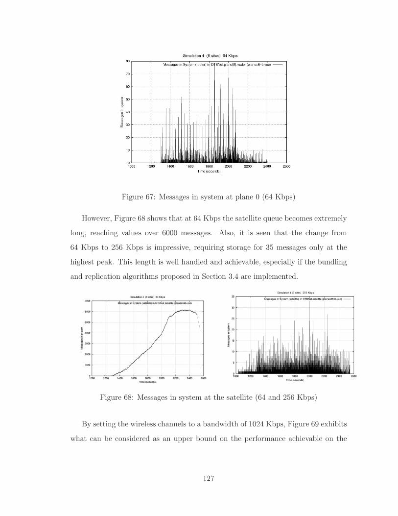
Figure 67: Messages in system at plane 0 (64 Kbps)
However, Figure 68 shows that at 64 Kbps the satellite queue becomes extremely
long, reaching values over 6000 messages. Also, it is seen that the change from
64 Kbps to 256 Kbps is impressive, requiring storage for 35 messages only at the
highest peak. This length is well handled and achievable, especially if the bundling
and replication algorithms proposed in Section 3.4 are implemented.
Figure 68: Messages in system at the satellite (64 and 256 Kbps)
By setting the wireless channels to a bandwidth of 1024 Kbps, Figure 69 exhibits
what can be considered as an upper bound on the performance achievable on the
127
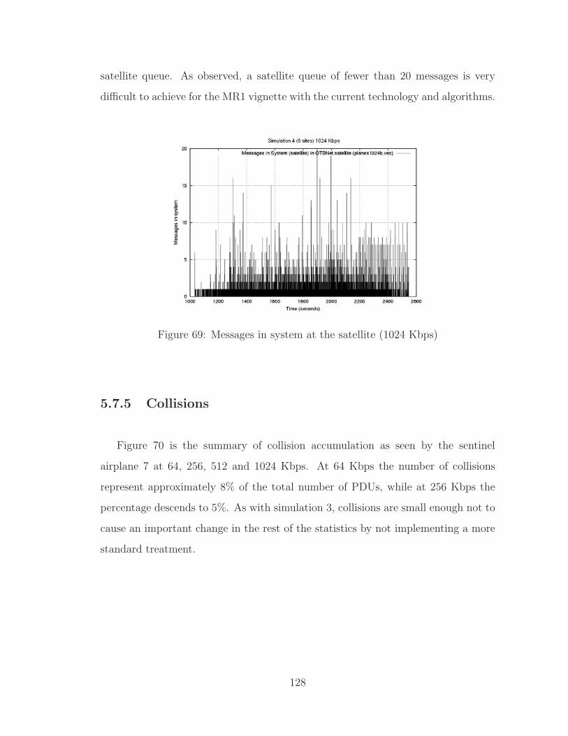
satellite queue. As observed, a satellite queue of fewer than 20 messages is very
difficult to achieve for the MR1 vignette with the current technology and algorithms.
Figure 69: Messages in system at the satellite (1024 Kbps)
5.7.5 Collisions
Figure 70 is the summary of collision accumulation as seen by the sentinel
airplane 7 at 64, 256, 512 and 1024 Kbps. At 64 Kbps the number of collisions
represent approximately 8% of the total number of PDUs, while at 256 Kbps the
percentage descends to 5%. As with simulation 3, collisions are small enough not to
cause an important change in the rest of the statistics by not implementing a more
standard treatment.
128
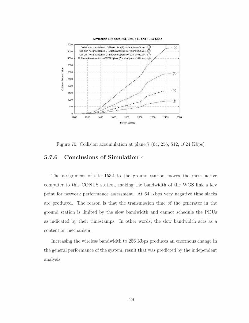
Figure 70: Collision accumulation at plane 7 (64, 256, 512, 1024 Kbps)
5.7.6 Conclusions of Simulation 4
The assignment of site 1532 to the ground station moves the most active
computer to this CONUS station, making the bandwidth of the WGS link a key
point for network performance assessment. At 64 Kbps very negative time slacks
are produced. The reason is that the transmission time of the generator in the
ground station is limited by the slow bandwidth and cannot schedule the PDUs
as indicated by their timestamps. In other words, the slow bandwidth acts as a
contention mechanism.
Increasing the wireless bandwidth to 256 Kbps produces an enormous change in
the general performance of the system, result that was predicted by the independent
analysis.
129

5.8 Simulation using Head of Line Strategy
HOL strategies are mentioned in the Ph.D. dissertation [Liu02], in the paper
[DGR01], and in the research papers [PW03] and [LS93], among many others.
130
CHAPTER 6
TRAFFIC OPTIMIZATION USING PDUAlloy
The analysis of negative spikes in Section 5.6.6 induced the idea of a possible
solution to eliminate or reduce them by means of bundling the participating PDUs
into a single packet. In order to do so, the PDUs were examined in more detail,
looking for similarities and redundancies in their fields.
Each type of PDU has its own internal structure made up of fields and values of
different sizes. A study of all the logged PDUs in the MR1 vignette indicated that
if two PDUs are of the same type and length then they have identical structure, as
indicated in Section 3.4.2. This is a key point in the proposed bundling algorithm.
Another observation from the logged PDUs is the fact that OTB schedules some
sequences of consecutive PDUs using exactly the same timestamp, as in the sample
sequence shown in Figure 56. This causes a bottleneck in generators due to the
impossibility of sending several packets at the same time. In most cases, consecutive
PDUs of equal type and length differed in the contents of some few fields, giving
the possibility of merging them into a single PDU.
6.1 Independent Analysis and Assignment of PDUs
The same input data from Simulations 3 and 4 is used in Simulation 5, and so
the independent analysis is exactly the same as in those simulations, reason why it
is omitted here.
131
The assignment of OTB sites to computer nodes in Simulation 5 is the same as
in Simulation 4, and can be found in Section 5.7.1.
6.2 Input Data
The summary PDU files described in Figure 19 of Section 5.2 contain 4 characters
at the end of each PDU. The characters are S standing for send, and W standing
for wait. They provide information about the action to follow after processing each
PDU. Six algorithms to predict that action are proposed and studied under this
Simulation 5. They can be classified in two groups: on-line algorithms, which decide
the next action based only on the already processed PDUs, and off-line algorithms,
which know all the past and future sequence of PDUs in advance.
In this simulation the on-line algorithms are neural-network prediction (see
details on Section 3.4.2.1), Always-Wait and Always-Send. The off-line ones are
type, type-and-length, and type-length-and-time, which have the capability of a perfect
prediction due to their knowledge of the future.
6.3 Slack Time
Figure 71 shows the slack time of the generator at the CONUS ground station
for different predictive algorithms.
The graph was created assigning 64 Kbps to all the wireless links and 100
milliseconds to the timeout period. As seen in the diagram, up to the second 1600
all of the algorithms behaved alike, but then negative slack started to build up. The
Always-Send algorithm, which is equivalent to the non-bundling algorithm used
in Simulation 4 (see Figure 62), incurred in the largest negative slack, followed
132
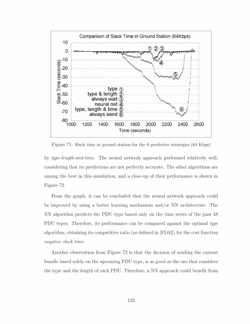
Figure 71: Slack time at ground station for the 6 predictive strategies (64 Kbps)
by type-length-and-time. The neural network approach performed relatively well,
considering that its predictions are not perfectly accurate. The other algorithms are
among the best in this simulation, and a close-up of their performance is shown in
Figure 72.
From the graph, it can be concluded that the neural network approach could
be improved by using a better learning mechanism and/or NN architecture. The
NN algorithm predicts the PDU type based only on the time series of the past 48
PDU types. Therefore, its performance can be compared against the optimal type
algorithm, obtaining its competitive ratio (as defined in [FL02]) for the cost function
negative slack time.
Another observation from Figure 72 is that the decision of sending the current
bundle based solely on the upcoming PDU type, is as good as the one that considers
the type and the length of each PDU. Therefore, a NN approach could benefit from
133
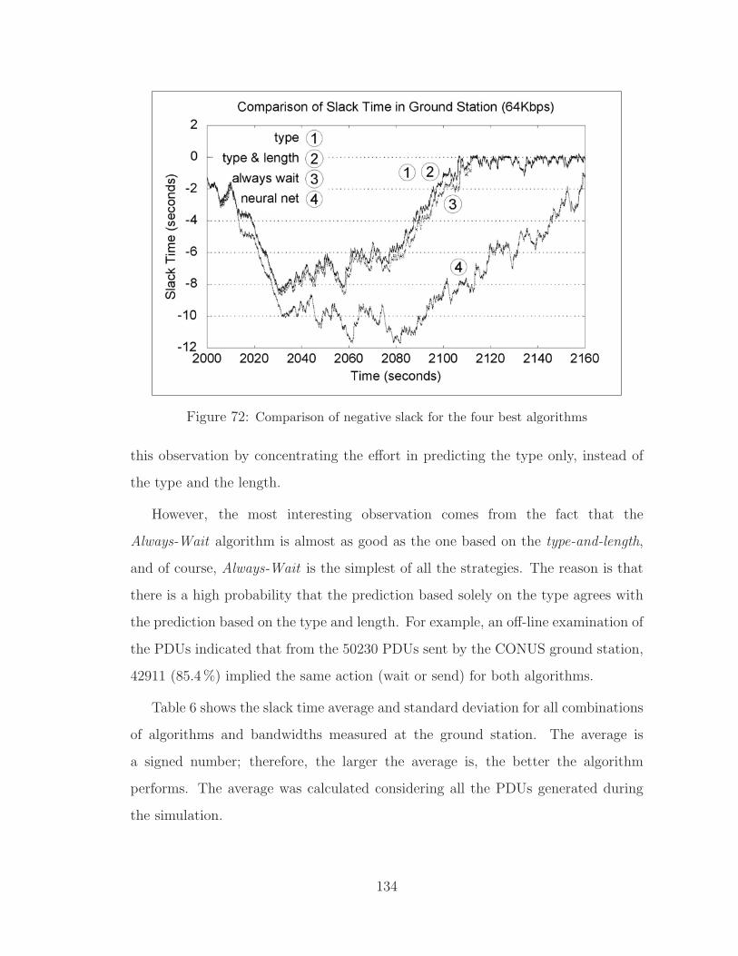
Figure 72: Comparison of negative slack for the four best algorithms
this observation by concentrating the effort in predicting the type only, instead of
the type and the length.
However, the most interesting observation comes from the fact that the
Always-Wait algorithm is almost as good as the one based on the type-and-length,
and of course, Always-Wait is the simplest of all the strategies. The reason is that
there is a high probability that the prediction based solely on the type agrees with
the prediction based on the type and length. For example, an off-line examination of
the PDUs indicated that from the 50230 PDUs sent by the CONUS ground station,
42911 (85.4 %) implied the same action (wait or send) for both algorithms.
Table 6 shows the slack time average and standard deviation for all combinations
of algorithms and bandwidths measured at the ground station. The average is
a signed number; therefore, the larger the average is, the better the algorithm
performs. The average was calculated considering all the PDUs generated during
the simulation.
134
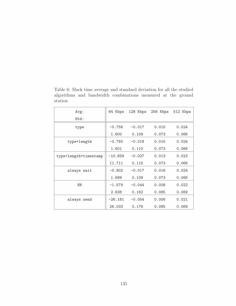
Table 6: Slack time average and standard deviation for all the studiedalgorithms and bandwidth combinations measured at the groundstation
Avg: 64 Kbps 128 Kbps 256 Kbps 512 Kbps
Std:
type -0.758 -0.017 0.015 0.024
1.600 0.109 0.073 0.066
type+length -0.760 -0.018 0.015 0.024
1.601 0.110 0.073 0.066
type+length+timestamp -10.659 -0.027 0.013 0.023
11.711 0.115 0.073 0.066
always wait -0.802 -0.017 0.016 0.024
1.689 0.109 0.073 0.066
NN -1.579 -0.044 0.008 0.022
2.638 0.162 0.085 0.069
always send -26.181 -0.054 0.006 0.021
26.033 0.176 0.085 0.069
135
From this table it is concluded that the Always-Send is the worst of the six
algorithms, and Always-Wait is among the best ones. Because, Always-Send
corresponds to the non-bundling option, it is inferred that the type of bundling
proposed is of advantage to the DIS protocol.
Another observation comes from the fact that at 64 and 128 Kbps, the average
slack time was negative for all the algorithms, but for 256 and above it is positive.
A negative average indicates that the corresponding bandwidth is insufficient to
handle the PDU traffic. Therefore, for the MR1 vignette, the wireless bandwidth
should be at least 256 Kbps.
6.4 Travel Time
Every time a bundle is sent, the current time (Tsend) is attached to it, allowing the
destinations to calculate the travel time Ttrav , as indicated in Equation 5.6. Figure
73 shows the travel time measured at sink 0 onboard plane 0, for the Always-Wait
strategy, using 64 and 128 Kbps in wireless links. It is clear from the graph that 64
Kbps is not enough bandwidth to handle all the traffic required by the simulation,
even with bundling. As seen, during the interval from second 2000 to second 2400
many of the PDUs took almost 40 seconds to arrive at their destinations, making the
OTB simulation useless. However, a big improvement is obtained just by duplicating
the bandwidth. At 128 Kbps, the latency was close to 0.8 seconds, as observed in
Figure 74.
Figure 74 shows that most of the PDUs take less than 0.4 seconds to reach their
destinations. It is interesting to note the large concentration of PDUs near 0.25
seconds, which is the propagation delay for satellite signals. The graph also shows
136
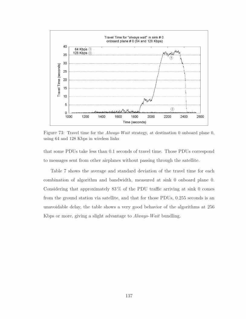
Figure 73: Travel time for the Always-Wait strategy, at destination 0 onboard plane 0,using 64 and 128 Kbps in wireless links
that some PDUs take less than 0.1 seconds of travel time. Those PDUs correspond
to messages sent from other airplanes without passing through the satellite.
Table 7 shows the average and standard deviation of the travel time for each
combination of algorithm and bandwidth, measured at sink 0 onboard plane 0.
Considering that approximately 83 % of the PDU traffic arriving at sink 0 comes
from the ground station via satellite, and that for those PDUs, 0.255 seconds is an
unavoidable delay, the table shows a very good behavior of the algorithms at 256
Kbps or more, giving a slight advantage to Always-Wait bundling.
137
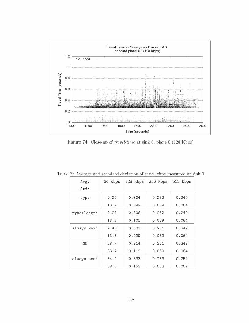
Figure 74: Close-up of travel-time at sink 0, plane 0 (128 Kbps)
Table 7: Average and standard deviation of travel time measured at sink 0
Avg: 64 Kbps 128 Kbps 256 Kbps 512 Kbps
Std:
type 9.20 0.304 0.262 0.249
13.2 0.099 0.069 0.064
type+length 9.24 0.306 0.262 0.249
13.2 0.101 0.069 0.064
always wait 9.43 0.303 0.261 0.249
13.5 0.099 0.069 0.064
NN 28.7 0.314 0.261 0.248
33.2 0.119 0.069 0.064
always send 64.0 0.333 0.263 0.251
58.0 0.153 0.062 0.057
138

6.5 Queue Length
Due to the nature of the PDU traffic in the simulation, two queues to focus
attention on are the router queue onboard any aircraft, for instance airplane 0, and
the satellite queue. Figure 75 shows the satellite queue at 64 and 128 Kbps.
Figure 75: Messages in satellite at 64 and 128 Kbps showing the impact of a higherbandwidth on its queue
It is clear from the graph that 64 Kbps is an insufficient bandwidth, causing the
satellite queue to grow unbounded. The reason for having a descent after reaching a
maximum of about 6000 messages, is that the simulation is approaching its end and
no more messages are sent from the generators. However, at 128 Kbps a significant
change in the queue length is produced, keeping it at reasonably low values.
Another observation is that at 64 Kbps the graph does not reach zero at the end.
This occurs because the queue status is reported only if another message enters the
queue. After the arrival of the last message to the queue, the messages are consumed
without being reported.
139
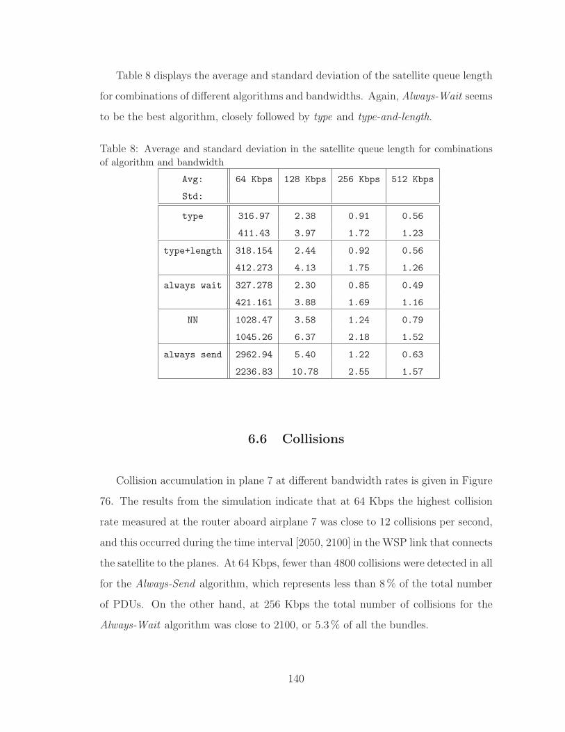
Table 8 displays the average and standard deviation of the satellite queue length
for combinations of different algorithms and bandwidths. Again, Always-Wait seems
to be the best algorithm, closely followed by type and type-and-length.
Table 8: Average and standard deviation in the satellite queue length for combinationsof algorithm and bandwidth
Avg: 64 Kbps 128 Kbps 256 Kbps 512 Kbps
Std:
type 316.97 2.38 0.91 0.56
411.43 3.97 1.72 1.23
type+length 318.154 2.44 0.92 0.56
412.273 4.13 1.75 1.26
always wait 327.278 2.30 0.85 0.49
421.161 3.88 1.69 1.16
NN 1028.47 3.58 1.24 0.79
1045.26 6.37 2.18 1.52
always send 2962.94 5.40 1.22 0.63
2236.83 10.78 2.55 1.57
6.6 Collisions
Collision accumulation in plane 7 at different bandwidth rates is given in Figure
76. The results from the simulation indicate that at 64 Kbps the highest collision
rate measured at the router aboard airplane 7 was close to 12 collisions per second,
and this occurred during the time interval [2050, 2100] in the WSP link that connects
the satellite to the planes. At 64 Kbps, fewer than 4800 collisions were detected in all
for the Always-Send algorithm, which represents less than 8 % of the total number
of PDUs. On the other hand, at 256 Kbps the total number of collisions for the
Always-Wait algorithm was close to 2100, or 5.3 % of all the bundles.
140

Figure 76: Collision accumulation at plane 7 (64, 256, 512, 1024 Kbps)
As Figure 76 shows, at 128 and 256 Kbps there is roughly a total difference of
1000 fewer collisions for the Always-Wait than for the Always-Send algorithm, which
indicates that bundling significantly reduces the number of collisions, given the same
bandwidth for both algorithms. In addition, it can be noted that as the bandwidth
increases, the number of collisions decreases, which is intuitively explained because
at higher bandwidths the packets take less transmission time, and so the probability
of a collision gets lower.
6.7 Conclusions of Simulation 5
The main conclusion of this simulation is that the type of bundling proposed in
this dissertation proved to be successful during the simulation of the MR1 vignette.
All the algorithms based on bundling performed a lot better than the non-bundling
Always-Send algorithm.
141
prediction based solely on the PDU type is almost as good as the prediction based
on the type and the length, and these predictions are better than the Always-Wait
algorithm by half a second in some cases. Therefore, a NN approach could be useful
if the percentage of successful guesses is so high that outperforms the Always-Wait
algorithm.
Another conclusion is that the Always-Wait algorithm, although not optimal,
gives very good results that can be acceptable in many cases, especially if the
bandwidth is incremented. Let’s take into account that the shown results are
simulations at 64 KBps. At higher bandwidths, the difference between Always-Wait
and the perfect guessing algorithms (type, type-and-length)becomes smaller, giving
the easy-to-program Always-Wait strategy a relevant importance.
The final conclusion about the bandwidth is that 256 Kbps in wireless channels
is the minimum bandwidth for the MR1 vignette that passes all the tests (slack
time, travel time, queue length, and collisions) in an acceptable way.
142

CHAPTER 7
CONCLUSIONS
There are three main sets of conclusions that can be drawn. The first set
corresponds to conclusions about the required bandwidth in the wireless channels
to carry out the OTB simulation. The second set corresponds to conclusions about
the effectiveness of the bundling techniques.
The simulation issues in this dissertation can be divided into three main
areas: re-scheduling and transmission of PDUs, replication and prediction of PDUs,
and PDU compression. In the following, each area is briefly addressed.
7.1 Scheduling
The re-scheduling and transmission of PDUs is an attempt to reduce the negative
slack spikes by transferring some of their PDUs to periods of positive slack. Not
only the po fire parameters PDUs are subject to be rescheduled, but any PDU
that involves some sort of negative slack could be reschedule. The goal is to obtain
a traffic as close as possible to a burst-free model to keep the channels busy but not
flooded.
The DIS protocol is responsible for the timestamps of the PDU packets. If many
PDUs are scheduled not only at the same microsecond, but also within a very short
time interval, the effect is similar to a negative spike. The experiments with the
OMNeT simulation showed that mixed with negative spikes there are many positive
143

ones. The positive spikes indicate that the channel is not used during those intervals
and so rescheduling of the PDUs could bring a better utilization of the channel. If
a sequence of PDUs timestamped at almost the same time followed by periods of
rest can be recognized and predicted, then the scheduler could implement a type of
contention to refrain from sending those PDUs so close to each other and spread
the sending times evenly throughout the intervals of low traffic. In doing so, the
length of each PDU must be taken into account because it is proportional to the
transmission time.
The proposed research will require access to the specific formats and
characteristics of PO PDUs. Also, the implicit assumption that in OTB some PDUs
can be rescheduled and be sent in a different order without adversely affecting the
overal simulation must be corroborated. If that is the case, we propose to identify
priority levels for PDUs.
It is possible to introduce modifications in the PDU scheduling aimed at reducing
the traffic by sending just one PDU in cases where several of them are sent at the
same timestamp.
The observations pointed out in the conclusions suggest that it is possible
to introduce modifications in the PDU scheduling aimed at reducing the traffic
by sending just one PDU in cases where several of them are sent at the same
timestamp. The idea is to investigate the possibility of introducing a kind of protocol
compression to eliminate redundancy in consecutive PDUs. For instance, if several
po fire parameters PDUs are sent, only one real PDU could actually be sent,
along with some new fields indicating the number of PDUs scheduled at this time
as well as an indication of the changes to be applied in order to extract the other
PDUs from the given one.
A side effect of reducing the PDU traffic is a decrease of collisions, especially
if the PDUs are relatively long, as is the case of po fire parameters PDUs. Ten
144
consecutive PDUs of this type account for 5280 bytes plus the time gaps between
frames. During the transmission time of these PDUs, the channels are heavily
occupied and any other attempt to transmit from another station over the same
channel will end up in a collision. By sending just one PDU of approximately 550
bytes will decrease the probability of having a collision.
po fire parameters PDUs can be successfully compressed under certain
conditions.
A side effect of reducing the PDU traffic is a decrease of collisions, especially
if the PDUs are relatively long, as is the case of po fire parameters PDUs. Ten
consecutive PDUs of this type account for 5280 bytes plus the time gaps between
frames. During the transmission time of these PDUs, the channels are heavily
occupied and any other attempt to transmit from another station over the same
channel will end up in a collision. By sending just one PDU of approximately 550
bytes will decrease the probability of having a collision.
The re-scheduling and transmission of PDUs is an attempt to reduce the negative
slack spikes by transferring some of their PDUs to periods of positive slack. Not
only the po fire parameters PDUs are subject to be rescheduled, but any PDU
that involves some sort of negative slack could be reschedule. to obtain a traffic as
close as possible to a burst-free model to keep the channels busy but not flooded.
The experiments with the OMNeT simulation showed that mixed with negative
spikes there are many positive ones. The positive spikes indicate that the channel
is not used during those intervals and so rescheduling of the PDUs could bring a
better utilization of the channel. If a sequence of PDUs timestamped at almost the
same time followed by periods of rest can be recognized and predicted, then the
scheduler could implement a type of contention to refrain from sending those PDUs
so close to each other and spread the sending times evenly throughout the intervals
of low traffic.
145
some PDUs can be rescheduled and be sent in a different order without adversely
affecting the overal simulation
Besides the common compression algorithms, another strategy to consider is the
concatenation of several consecutive PDUs scheduled during very short periods of
time. The time gap between packets is also a variable to consider. It is possible to
save TCP/IP headers and inter-packet time gaps by assembling together individual
PDUs into a large compact block. If the size of the largest acceptable block is
known, the problem of assembling shorter PDUs is twofold. First, a new set of
PDUs is collected and concatenated as long as the total size does not surpass the
block length. Second, while waiting for the next PDU a decision must be made
regarding the convenience of sending this block right now, or keep waiting for a
while. Here, the possibility of predicting the timestamp of the next PDU is a big
help to this decision. Some pattern recognition techniques could be applied to
predict a sequence of very close PDUs followed by a positive spike.
7.1.1 Required Bandwidth
The goal behind the development of this research was to estimate the required
bandwidth in the wireless channels for the effective communication of the OTB
modules in the flying network depicted in Figure 1. The LAN segments were
assumed Ethernet at 100 Mbps.
A vignette was prepared and run by OTB, simulating the 24 flying sites plus
the ground station. The PDU traffic generated was captured and used as input to
the OMNeT simulator, preserving the original timestamps, types and lengths. The
OMNeT simulator was run under several combinations of wireless bandwidths (64,
146
128, 256, 512, 1024 Kbps) and bundling techniques (Always-Send, neural network,
type, type+length, Always-Wait).
From the results of the OMNeT simulation, it is concluded that 64 Kbps in
the wireless links are not enough to handle the PDU traffic, due to the enormous
negative slack reported in the generators (Figure 71), the big travel time latency
reported in Figure 73, and the long satellite queue shown in Figure 75. However, at
128 Kbps the scenario changes dramatically, and at 256 Kbps it gets even better.
It seems that an average of 0.26 seconds in the travel time and 2.3 messages in the
satellite queue are good indicators of performance. However, the negative average
of -0.017 seconds indicates that 128 is not really enough bandwidth. Therefore,
the conclusion is that the required bandwidth should be at least 256 Kbps in the
wireless links.
The independent analysis performed on the logged data is an important
procedure in the assessment of bandwidth because it gives a good initial insight
about the minimum instant bandwidth required at a fraction of the cost of a
complete simulation. It can be used also to identify periods of low and high network
traffic, and correlate them with actions being developed by the simulated parties for
a better understanding of the simulation behavior.
7.1.2 Effectiveness of bundling
All of the statistics presented indicate that bundling is an effective technique
for reducing the PDU traffic and better utilize the bandwidth. The reductions in
negative slack (Figures 71 and 72), travel time (Table 7), satellite queue length
(Table 8), and number of collisions (Figure 39) are all indicators in that sense.
147

The replication of PDUs through bundling presented in this research differs from
other proposals [US95a, Tay95, Tay96b, Tay96a, Ful96, BCL97, PW98, WMS01] in
several ways. First, bundling takes into account the internal structure of each PDU;
only PDUs of the same type and length are put together in a bundle. Second, the
resulting bundle has a structure similar to any other PDU and can be considered
a PDU of a different type, subject to further bundling or compression technique if
desired. Third, the bundling algorithm is simple and easy to implement, as well as
the extraction of individual PDUs at the destination. Each bundle is independent
of the others and all the information needed to extract the PDUs is contained in
the same bundle. A previous basic PDU sent to the destinations containing static
values is not used in this approach.
The bandwidth analysis showed that, on the average 256 Kbps in the wireless
channels are sufficient to handle the traffic of experiments 1 and 2 corresponding to
the contracted vignette, except for the negative spikes of the slack time detected at
the sending stations.
The main cause of those negatives spikes is the scheduling of PDUs having exactly
the same timestamp. The analysis of the largest spikes showed that PDUs of type
po fire parameters are the main components of those spikes and sequences of 8 or
more PDUs are common. Each po fire parameters PDU has a length of 528 bytes.
Comparisons of samples of po fire parameters PDUs for the same spike indicated
that they are very similar, having differences related to PDU identification and
memory address of the PDU fields only. Other types of PDUs scheduled at exactly
the same timestamp have not been investigated yet, but it is quite possible that
PDUs of the same type bearing the same timestamp are very similar.
In Simulation 1 ... as predicted, 64 Kbps in the wireless links is insufficient to
handle Embedded Training traffic under a DIS-like protocol. Latencies of more than
70 and 100 seconds, respectively, were detected for traffic from simulation stations
148
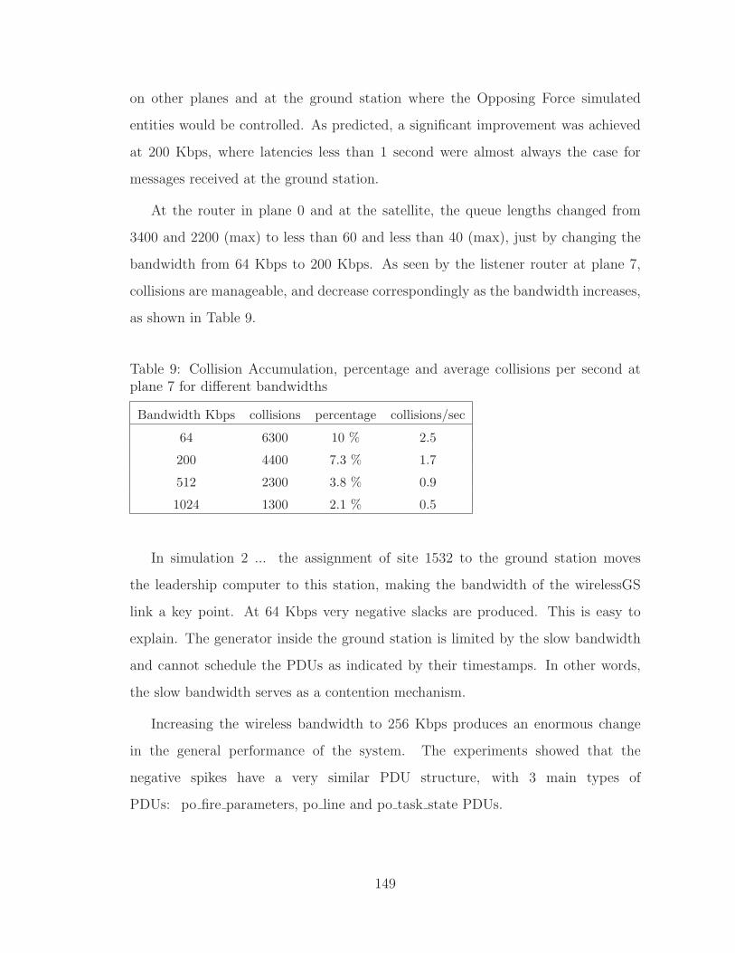
on other planes and at the ground station where the Opposing Force simulated
entities would be controlled. As predicted, a significant improvement was achieved
at 200 Kbps, where latencies less than 1 second were almost always the case for
messages received at the ground station.
At the router in plane 0 and at the satellite, the queue lengths changed from
3400 and 2200 (max) to less than 60 and less than 40 (max), just by changing the
bandwidth from 64 Kbps to 200 Kbps. As seen by the listener router at plane 7,
collisions are manageable, and decrease correspondingly as the bandwidth increases,
as shown in Table 9.
Table 9: Collision Accumulation, percentage and average collisions per second atplane 7 for different bandwidths
Bandwidth Kbps collisions percentage collisions/sec
64 6300 10 % 2.5
200 4400 7.3 % 1.7
512 2300 3.8 % 0.9
1024 1300 2.1 % 0.5
In simulation 2 ... the assignment of site 1532 to the ground station moves
the leadership computer to this station, making the bandwidth of the wirelessGS
link a key point. At 64 Kbps very negative slacks are produced. This is easy to
explain. The generator inside the ground station is limited by the slow bandwidth
and cannot schedule the PDUs as indicated by their timestamps. In other words,
the slow bandwidth serves as a contention mechanism.
Increasing the wireless bandwidth to 256 Kbps produces an enormous change
in the general performance of the system. The experiments showed that the
negative spikes have a very similar PDU structure, with 3 main types of
PDUs: po fire parameters, po line and po task state PDUs.
149
It seems that the sequence mainly responsible of negative spikes is of type
po fire parameters, perhaps because the entity studied (ground station) is firing
against some enemy. This hypothesis needs to be corroborated against an actual
run of the OTB vignette. If the hypothesis is corroborated, then it can be concluded
that firing activities cause those spikes.
Also, although not a universal contribution, through this research the Electrical
and Computer Engineering Department of the University of Central Florida got
familiar with the OMNeT software, which is in the public domain and provides a
quality simulation environment for C++ programmers. The development of the
simulator for handling PDUs of an OTB application is an example of OMNeT usage
that can serve as a starting basis for other projects.
150

CHAPTER 8
FUTURE WORK
8.1 Future Work
Better NN predictive algorithm. Another branch of research could be based on
the prediction of the type for the upcoming PDUs. The neural network developed
in this study was very simple, having an accuracy of prediction close to 70 %. If
an improved neural network is developed, it could beat the Always-Wait strategy.
However, a careful comparison in terms of simplicity and usage of CPU time and
memory between both algorithms would be required.
Specific format of PO PDUs, not only regular PDUs, must be studied and
incorporated in the bundling strategies.
we propose to identify priority levels for PDUs. By using Head-of-Line (HOL)
queueing service strategies such that high priority PDUs are put at the front of
the queue, the critical PDUs will be scheduled on time for the consistency of the
simulation.
technique that can be used to diminish negative spikes and in general make a
better usage of the available bandwidth is related to data compression. Compression
can be applied at two levels: data compression of the PDU data, and compression
of the TCP/IP headers.
Several possibilities of future work are open. The bundling algorithm could be
extended to consider PDUs of the same type but different length as candidates to
151

be included in the bundle. Also, the bundling of PDUs of different types could also
be researched as long as the resulting bundle still keeps the structure of a PDU.
The bundling strategy aimed at preserving the message structure could be
applied to other communication protocols or data streams besides DIS. For instance,
if a large database needs to be transmitted through a slow network and the
records have some sequence relationship such that repeated fields are often found in
consecutive records, the records could be bundle using the algorithms presented in
this article.
The implementation of the said PDU compression and rescheduling techniques
could be made inside OTB directly, or by appending a filter to the OTB output,
together with a de-filter module at the receiving site. The filter has the advantage of
not modifying the current OTB implementation, at a cost of less efficiency. But for
the goals of this research, it is enough to demonstrate that the proposed techniques
are reasonable and achievable.
It must be investigated whether the compression of PDUs can be done by
extending the current PDUs with new fields, or by creating a new PDU type with
the new fields, and then send it as a prefix to the PDU that will be expanded.
An additional product obtainable from the project is the development and
maintainability of UCF OMNeT++ models and logger files based on generic libraries
suitable for FCS capacity planning and requirements generation. A self-contained
executable demo is a valuable help for future presentations of the project.
152

APPENDIX A
MR1 VIGNETTE
153
APPENDIX A
MR1 VIGNETTE
This vignette is due to Dr. Avelino Gonzalez and Dr. Michael Georgiopoulos.
A.1 Background
In 2014, twenty years of independence for the Trans-Caucasus States found
serious socio-political, ethno-religious, and economic conflict spreading throughout
the region. Azerbaijan emerged as the leading economic power through the
exploitation of Caspian and Central Asian oil reserves. Azerbaijan’s politics were
deeply divided; its citizens and Karabakh refugees demanded the government take
military action against the Armenian Karabakh that forced them to flee. The
Azerbaijani government refused to act, and refugees from the Nagorno-Karabakh
Internal Liberation Organization [NKILO], using terror and armed force to achieve
their goals, began a cross-border unconventional campaign designed to force a
confrontation between the two countries. Observing these developments, Armenia
and Iran viewed the Azerbaijani government’s instability as an opportunity to
expand their influence in the region for political gain. Armenia began massing
maneuver forces along the Azerbaijani border and repositioned mobile Theater
Ballistic Missile launchers. Both countries perceived a low risk of failure in executing
their campaign strategy and were willing to impose a military solution upon the
Azerbaijani problem.
154
In November 2014, initial reports of the Caspian Sea Peninsula crisis caused the
U.S. to take steps to improve its awareness of the developing situation. The Secretary
of Defense redirected intelligence assets to focus on the region and directed political
and military planners to formulate contingency plans for U.S. engagement in the
region. They determined an Army Objective Force Unit of Employment 2, operating
as the Army component of a joint force, would be required to accomplish U.S. goals
in the region and assigned operational control of the 15th Division air-ground task
force to USEUCOM for planning purposes. Warning orders were issued through
USEUCOM to the U.S. 15th Division air-ground task force, and supporting attack
and lift aviation assets to begin their own planning. US Army Europe (USAREUR)
and its theater support command (TSC) reviewed and updated contingency plans
and refined the sustainment preparation of the theater. The TSC issued warning
orders and created a provisional logistics/sustainment task organization called the
Area Support Group (ASG) that would support land forces employed in theater.
In late November, the Azeri Islamic Brotherhood (AIB), a coalition of
anti-government factions supported by NKILO and the Azerbaijani National Front
for Revolutionary Action (ANFRA) military forces, subverted the bulk of an Azeri
Motorized Rifle Brigade, which mutinied to realign with this faction. The brigade
seized control of most of the historically significant Icheri Sheher (Inner Town)
district in Baku. However, a desperate defense by loyal government forces managed
to secure the centers of government within the capital city. Meanwhile, two
armed clan-based factions of the Azeri Islamic Brotherhood, the Aziz and Daha,
extended their control of the eastern and western outskirts of Baku, respectively,
and intensified their efforts to overthrow the legitimate government. As a last resort,
the Azerbaijani government requested assistance from the Russian Federation to
defeat the insurgents and preclude an anticipated invasion by Armenian forces. On
15 December, Russia proposed a coalition of U.S. and Russian forces to restore
155
order within Azerbaijan and stabilize the government. Two days later, the U.S.
agreed to the proposal and the two nations created a coalition force and outlined its
employment plan. The joint force commander, United States European Command
(USEUCOM), and his Russian counterpart formed a coalition staff that included a
coalition/joint theater logistics management element (C/JTLME). The C/JTLME
continued to develop plans to logistically support coalition forces employed in theater
and to determine the most efficient use of all coalition movement, sustainment, and
facilities assets.
United States European Command focused its main effort at developing the
situation and expanding the knowledge base already resident from the Operational
Net Assessment of this region. They pre-positioned incremental force packages
to establish a military presence in the region and deter any further hostilities,
establishing a C4ISR architecture, and posturing to project forces directly into
Azerbaijan and to dismantle Armenian C4ISR and fires systems. The combatant
commander deployed Special Operations Forces (SOF) into the region, adding an
additional layer of intelligence collection assets to the national-level space and
air-based assets already operating over the region. Initially, their efforts were focused
on developing the situation in the region of the beleaguered government in Baku.
But as the 15th Division matured its plans, SOF teams shifted to provide coverage
of the airfields the 15th Division planned to use as tactical points of entry for one
brigade-sized Unit of Action (UA), the 1st Brigade UAs. The 1st Brigade UA is
composed of three Battalions, the 1st, 2nd and 3rd.
A.2 General Vignette Description
This section describes the vignette in detail. It focuses on the 3rd battalion of
the 1st Brigade Unit of Action. More specifically, it focuses on the lead element of
156
the 3rd battalion - the Alpha Company. This company comes upon fortified defenses
of the ANFRA forces and must destroy them to make way for the main element of
the 3rd battalion coming up behind them. This is described in this section.
A.2.1 Situation and Mission Prior to Start of Vignette
The 1st and 2nd Battalions of the 1st Brigade UA are already on the ground
before the beginning of this vignette. They have attacked the enemy forces in the
city of Baku, defeated the subverted Azer brigade that controlled the City Center
(referred to as the Icheri Sheher Brigade). Moreover, they confronted and routed
the AIB forces in the vicinity of Baku. The 1st Battalion was subsequently tasked
with pursuing the withdrawing AIB enemy forces retreating towards Agdam, and
to continue on to Agdam and occupy it. The 2nd Battalion was ordered to maintain
pressure on the Icheri Sheher Brigade in Baku to defeat it in detail.
In the meantime, 300 Km to the west, ANFRA forces, attacked across the
Armenian border, seized the city of Agdam, and continued eastward to join with the
retreating AIB forces and attempt to relieve the beleaguered Icheri Sheher Brigade
in Baku. However, surprised by the rapid defeat of their allies in Baku, the ANFRA
forces suddenly found themselves in an exposed position in the wide river valley
between Agdam and Baku. Aware that the US forces (the 1st Brigade UA) were
mounting an operation to move westward to secure Agdam and restore the border,
ANFRA forces began a delaying operation, designed to buy time for establishing a
defense of Agdam while slowing and inflicting casualties on the attacking US force.
Keys to their hopes of success were preservation of the delaying force and effective
use of target acquisition systems linked to long-range artillery systems.
157
The 3rd Battalion of the 1st UA Brigade now comes into the picture in this
vignette with orders to attack and destroy the delaying forces of the ANFRA in
order to permit the 2nd battalion to complete its mission of recapturing Agdam.
The 3rd Battalion is in the midst of an airlift operation from a transfer point in
Turkey when its specific mission is given to the commander. It must land, stage the
assets, organize itself and very rapidly move to accomplish its objective. Speed in
this mission is of the essence.
A.2.2 The 1st UA Prepares for Entry Operations
The commander of the 3rd Battalion, on the way to the AOR via an airlift operation,
was given a warning order to prepare to deploy immediately upon landing, and
attack and destroy the delaying forces of the ANFRA. If successful, this would permit
the 2nd Battalion of the 1st UA Brigade to complete its mission. The commander
of the 1st UA used information from coalition/joint theater logistics management
element (C/JTLME) fused with intelligence reporting from airborne assets and SOF
teams operating in the area to select one airfield in vicinity of Baku (60 Km NW of
the city) as his planned point of entry, as shown in Figure 1.
3.3 Mounted Formation Conducts Pursuit and Exploitation
Shortly after landing in their designated entry points, the 3rd Battalion of the
1st UA reorganizes and moves towards the ANFRA forces in open rolling terrain
with some variance of complexity, such as defiles and small villages. The enemy is
a combination of conventional forces, paramilitary, and special police challenging
the UA forces with both direct military combat engagements and asymmetric
means. The 3rd Battalion moves to contact with the ANFRA forces with the intent
to maintain pressure on delaying forces, dislocate them, and force them into a
158
battle while moving through open and rolling terrain so they could be destroyed
by assault. To minimize his vulnerability to the enemy’s long-range artillery
systems, the commander planned to move his battalion dispersed on multiple axes
while fighting an aggressive counter-reconnaissance effort. The result was near
autonomous operations by each company, a common operating picture enhanced by
situational awareness and networked fires ensured the force remained interdependent
and mutually supporting.
A.3 Specific Vignette for Project
As the 3rd Battalion of the 1st brigade UA advanced rapidly to meet the flank of
the delaying force, the aviation detachment identified an enemy defensive position
60 Km in advance of the 3rd Battalion’s lead elements (the Alpha company).
The position was carefully selected by ANFRA forces to protect the AIB force
withdrawing from Baku. The positions overlooked the best approaches to a river
crossing along their line of withdrawal. Knowing that the lead Company (Alpha)
would close on the reported location in just over an hour, the aviation unit used its
sensors to identify specific target locations within the enemy position. Other sensors,
mounted on unmanned aerial vehicles (UAV), were diverted from other areas to
further develop the common operational picture. Their observations revealed that
the position was well defended by a combination of dismounted infantry elements,
Draega tanks, and Garm missile launchers in hastily prepared survivability positions.
Minefields protecting the position from direct assault were still incomplete and
operators of the advanced sensors on UAVs observing the area located several
exploitable gaps and ensured they were portrayed on the common operational picture
(COP). The scenario is depicted in Figure 77.
159
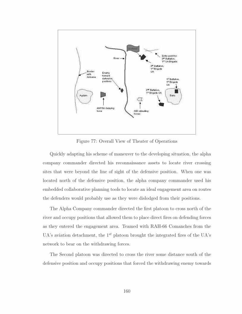
Figure 77: Overall View of Theater of Operations
Quickly adapting his scheme of maneuver to the developing situation, the alpha
company commander directed his reconnaissance assets to locate river crossing
sites that were beyond the line of sight of the defensive position. When one was
located north of the defensive position, the alpha company commander used his
embedded collaborative planning tools to locate an ideal engagement area on routes
the defenders would probably use as they were dislodged from their positions.
The Alpha Company commander directed the first platoon to cross north of the
river and occupy positions that allowed them to place direct fires on defending forces
as they entered the engagement area. Teamed with RAH-66 Comanches from the
UA’s aviation detachment, the 1st platoon brought the integrated fires of the UA’s
network to bear on the withdrawing forces.
The Second platoon was directed to cross the river some distance south of the
defensive position and occupy positions that forced the withdrawing enemy towards
160

the engagement area. The remaining two platoons were ordered to attack the enemy
position and compel the defending forces to withdraw, enabling their defeat in detail.
Still 30 km from the enemy position, the alpha company commander reviewed the
continuously updated common operational picture (COP) for obstacles along his
intended axis of advance. While he watched, a newly identified minefield was posted
on the display. Using the same planning tools, he quickly determined new routes
for each of his platoons, directing them towards bypasses around the minefield,
using line-of-sight evaluation tools to ensure the force stayed out of the enemy’s
line-of-sight as they maneuvered around the flank of the defending forces. Figure
78 provides detail about the target defensive positions as well as the crossing points
for the 1st and 2nd platoons.
Figure 78: Details of attack on defensive positions of ANFRA
When they closed to a range of 12 km, the alpha company’s mortars began the
attack on the defensive position. Pulling pin-point targeting data from the common
161
operational picture, they delivered precision munitions aimed directly at the vehicles
defiladed in the survivability positions within the enemy’s defense. Their lethal,
top-attack munitions quickly destroyed all but five vehicles.
Still too far away to directly observe the enemy positions, the Alpha Company
commander used the split screen option on his display to watch both the map
display of the common operational picture and live-video feed from the unmanned
aerial vehicles observing the enemy’s position. He watched as the five surviving
vehicles, three Draega tanks and two Garm missile launchers, left their positions
to flee towards Agdam, leaving the remaining dismounted defenders easy prey for
the mounted supported by dismounted combined arms assault that was to follow.
The icons on his common operational picture display indicated the fleeing vehicles
had taken an unanticipated route and were going to bypass the planned engagement
area. The commander quickly redirected the UAV to reconnoiter a route that his
display indicated would allow his 1st platoon to outflank the retreating vehicles while
he pursued them with his remaining two platoons.
With the reconnaissance of the UAV assuring the route was clear of obstacles,
the 1st platoon advanced rapidly and quickly overtook the fleeing enemy vehicles.
Two of the enemy tanks were destroyed with direct fire while the platoon moved
parallel to the fleeing enemy force, but the remaining three vehicles found cover
behind a low ridge that separated the two forces. Using his embedded planning
tools, the 1st platoon leader quickly identified a position in advance of the moving
forces that would give him clear shots. Accelerating to speeds of 60 Km/h, the
platoon darted in front of the enemy and was there waiting as they crested the ridge
and employed direct fire to destroy these enemy forces. With the last of the enemy
vehicles confirmed destroyed, the platoon leader ordered the platoon into a traveling
over watch formation and continued movement to the west. Figure 79 depicts the
mentioned scenario.
162

Figure 79: Details of advances on the defensive positions after mortal fire
Though the remainder of the company was still beyond his direct observation,
his Common Operational Picture (COP) display assured him they were moving on
parallel routes and that he was well within the supporting range of their fires as
well as those of the battalion’s mortars. As they moved towards Agdam, embedded
logistics planning tools that had monitored the unit’s ammunition usage in the
recent engagement automatically transmitted an update to the battalion’s logistics
center. This constantly updated flow of information enabled the battalion staff to
effectively plan en-route re-supply operations that allowed the battalion to maintain
its momentum as they continued their pressure on the delaying enemy forces.
In summary, the 1st platoon overtakes and destroys the retreating tanks and
missile launchers. The 3rd and 4th platoon force the remaining dismounted enemy
forces in the defensive position to flee into the path of the 2nd platoon, ensuring their
surrender/destruction. The success in overcoming the defensive position enabled
163

the main elements of the 3rd battalion (Bravo and Echo companies) to overtake the
main elements of the ANFRA delaying forces and engage them into a pitched battle,
defeating them.
164
APPENDIX B
NED SOURCE CODE
165
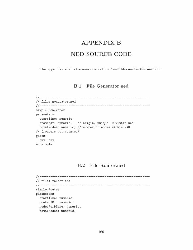
APPENDIX B
NED SOURCE CODE
This appendix contains the source code of the “.ned” files used in this simulation.
B.1 File Generator.ned
//-------------------------------------------------------------// file: generator.ned//-------------------------------------------------------------simple Generatorparameters:
startTime: numeric,fromAddr: numeric, // origin, unique ID within WANtotalNodes: numeric; // number of nodes within WAN
// (routers not counted)gates:
out: out;endsimple
B.2 File Router.ned
//-------------------------------------------------------------// file: router.ned//-------------------------------------------------------------simple Routerparameters:
startTime: numeric,routerID : numeric,nodesPerPlane: numeric,totalNodes: numeric,
166
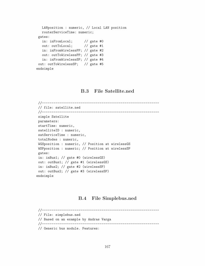
LANposition : numeric, // Local LAN positionrouterServiceTime: numeric;
gates:in: inFromLocal; // gate #0out: outToLocal; // gate #1in: inFromWirelessPP; // gate #2out: outToWirelessPP; // gate #3in: inFromWirelessSP; // gate #4
out: outToWirelessSP; // gate #5endsimple
B.3 File Satellite.ned
//-------------------------------------------------------------// file: satellite.ned//-------------------------------------------------------------simple Satelliteparameters:startTime: numeric,satelliteID : numeric,satServiceTime : numeric,totalNodes : numeric,WGSposition : numeric, // Position at wirelessGSWSPposition : numeric; // Position at wirelessSPgates:in: inBus1; // gate #0 (wirelessGS)out: outBus1; // gate #1 (wirelessGS)in: inBus2; // gate #2 (wirelessSP)out: outBus2; // gate #3 (wirelessSP)endsimple
B.4 File Simplebus.ned
//-------------------------------------------------------------// File: simplebus.ned// Based on an example by Andras Varga//-------------------------------------------------------------// Generic bus module. Features:
167

// - propagation delay modelling (proportional to distance)// - data rate modelling// - optional collision modeling// - optional collision signalling (if turned off, collided// frames are simply discarded// - full duplex or half duplex (simplex) bus. On a full duplex// bus, frames are assumed to propagate in one direction only// (upstream or downstream), and transmissions of opposite// directions don’t collide.// - models several independent channels//// Usage:// Set the parameters of the bus module and connect the stations// to it. Each station is expected to have a "position" attribute// which holds the station’s distance from one end of the bus.// There should be NO data rate set for the connecting links!//// Frames may have "channel" and "upstream" attributes; if they// are not present, the default values are 0 and TRUE. "upstream"// is only significant on a full duplex bus.//// The cMessages sent to the bus are interpreted as the start// of a transmission. Length of transmission is calculated from// the frame length and the bus data rate.//// The cMessages send out by the bus should be interpreted as the// _end_ of the transmission. Collision signal is an empty cMessage// with the name "collision". simple SimpleBusparameters:busType: string, // Types are: LAN, WPP, WSP, WGS.
numChannels, // number of independent channelswantCollisionModeling, // collision modeling flagwantCollisionSignal, // "send collision signals" flagisFullDuplex, // channel modedelaySecPerMeter, // delay of the busdataRateBps, // data rate of the busgapTime; // minimum gap between consecutive packets.
gates:in: in[ ];out: out[ ];
endsimple
168
B.5 File Sink.ned
//-------------------------------------------------------------// file: Sink.ned//-------------------------------------------------------------simple Sinkgates:
in: in;endsimple
B.6 File TheNet.ned
//-------------------------------------------------------------// file: theNet.ned//-------------------------------------------------------------import "generator.ned";import "simplebus.ned";import "sink.ned";import "router.ned";import "satellite.ned";// ------------ Module GroundStation -------------------------// module GroundStationparameters:
nodeID : numeric,WGSposition : numeric;
gates:out: out;in: in;
submodules:gen: Generator;parameters:
startTime = ancestor startTime,fromAddr = nodeID,totalNodes = ancestor nodesPerPlane * ancestor numPlanes;display: "i=gen;p=120,49;b=32,30";sink: Sink;display: "i=sink;p=81,49;b=32,30";
connections:gen.out --> out;sink.in <-- in;display: "p=18,2;b=176,102";
169
endmodule
// ---------- Module computer Node -------------------------module Nodeparameters:nodeID : numeric,LANposition : numeric;gates:out: out;in: in;submodules:gen: Generator;parameters:startTime = ancestor startTime,fromAddr = nodeID,totalNodes = ancestor totalNodes;display: "i=gen;p=120,49;b=32,30";sink: Sink;display: "i=sink;p=81,49;b=32,30";connections:gen.out --> out;sink.in <-- in;display: "p=18,2;b=176,102";endmodule
// ------------------ Module Plane -------------------------// module Planeparameters:
planeID : numeric,nodesPerPlane : numeric,totalNodes : numeric,WPPposition : numeric,WSPposition : numeric,routerServiceTime : numeric;
gates:in: inFromWirelessPP;out: outToWirelessPP;in: inFromWirelessSP;out: outToWirelessSP;
submodules:router: Router;
parameters:startTime = ancestor startTime,routerID = planeID,nodesPerPlane = nodesPerPlane,
170
totalNodes = totalNodes,LANposition = 10 * nodesPerPlane,routerServiceTime = routerServiceTime;display: "i=router;p=123,49;b=32,32";
//- - - - - - - - - - - - - - - - - - - - - - - - -node: Node[nodesPerPlane];parameters:
nodeID = planeID*nodesPerPlane + index,LANposition = 10 * index;display: "b=38,32;p=43,151,row,45;i=pc";
//- - - - - - - - - - - - - - - - - - - - - - - - -ethernetBus: SimpleBus;parameters:
busType = "LAN",numChannels = 1,wantCollisionModeling = 1,wantCollisionSignal = 1,isFullDuplex = 0,delaySecPerMeter = ancestor LANdelay,dataRateBps = ancestor LANbandwidth,gapTime = ancestor LANgapTime;
gatesizes:in[nodesPerPlane + 1],out[nodesPerPlane + 1];display: "p=88,97;b=156,10,rect";
//- - - - - - - - - - - - - - - - - - - - - - - - - - -connections:router.outToLocal --> ethernetBus.in[nodesPerPlane];router.inFromLocal <-- ethernetBus.out[nodesPerPlane];router.outToWirelessPP --> outToWirelessPP;router.inFromWirelessPP <-- inFromWirelessPP;router.outToWirelessSP --> outToWirelessSP;router.inFromWirelessSP <-- inFromWirelessSP;for i=0..nodesPerPlane-1 donode[i].out --> ethernetBus.in[i];node[i].in <-- ethernetBus.out[i];endfor;display: "p=2,2;b=168,184";endmodule
// ----------------- Module TheNet -------------------------module TheNetparameters:startTime : numeric,nodesPerPlane : numeric,
171
numPlanes : numeric,
LANgapTime : numeric,LANbandwidth : numeric,LANdelay : numeric,
WPPgapTime : numeric,WPPbandwidth : numeric,WPPdelay : numeric,
WSPgapTime : numeric,WSPbandwidth : numeric,WSPdelay : numeric,
WGSgapTime : numeric,WGSbandwidth : numeric,WGSdelay : numeric,
satServiceTime : numeric,routerServiceTime : numeric;submodules://- - - - - - - - - - - - - - - - - - - - - - - - -plane: Plane[numPlanes];parameters:
planeID = index,nodesPerPlane = nodesPerPlane,WPPposition = 100 * index,WSPposition = 100 * index,totalNodes = nodesPerPlane * numPlanes,routerServiceTime = routerServiceTime;display: "i=airplane;p=62,90,row,60;b=35,35";
//- - - - - - - - - - - - - - - - - - - - - - - - -wirelessPP: SimpleBus;parameters:busType = "WPP",numChannels = 1,wantCollisionModeling = 1,wantCollisionSignal = 1,isFullDuplex = 0,delaySecPerMeter = WPPdelay,dataRateBps = WPPbandwidth,gapTime = WPPgapTime;
gatesizes:in[numPlanes],out[numPlanes];
172
display: "p=264,33;b=476,10,rect";//- - - - - - - - - - - - - - - - - - - - - - - - -wirelessSP: SimpleBus;parameters:
busType = "WSP",numChannels = 1,wantCollisionModeling = 1,wantCollisionSignal = 1,isFullDuplex = 0,delaySecPerMeter = WSPdelay,dataRateBps = WSPbandwidth,gapTime = WSPgapTime;
gatesizes:in[numPlanes+1],out[numPlanes+1];display: "p=268,153;b=468,10,rect";
//- - - - - - - - - - - - - - - - - - - - - - - - -wirelessGS: SimpleBus;parameters:
busType = "WGS",numChannels = 1,wantCollisionModeling = 1,wantCollisionSignal = 1,isFullDuplex = 0,delaySecPerMeter = WGSdelay,dataRateBps = WGSbandwidth,gapTime = WGSgapTime;
gatesizes:in[2],out[2];display: "p=272,281;b=476,10,rect";
//- - - - - - - - - - - - - - - - - - - - - - - - -groundStation: GroundStation;parameters:
nodeID = nodesPerPlane * numPlanes,WGSposition = 0;display: "b=32,32;p=67,215,row,45;i=ground";
//- - - - - - - - - - - - - - - - - - - - - - - - -satellite: Satellite;parameters:
startTime = startTime,satelliteID = 1,satServiceTime = satServiceTime,totalNodes = nodesPerPlane * numPlanes,WSPposition = 38300E3, //35800 Km + 2500 Km
173

WGSposition = 38300E3; //35800 Km + 2500 Kmdisplay: "i=satellite;p=315,217;b=32,32";
//- - - - - - - - - - - - - - - - - - - - - - - - - - -connections:for i=0..numPlanes-1 do
plane[i].outToWirelessPP --> wirelessPP.in[i];plane[i].inFromWirelessPP <-- wirelessPP.out[i];plane[i].outToWirelessSP --> wirelessSP.in[i];plane[i].inFromWirelessSP <-- wirelessSP.out[i];
endfor;groundStation.out --> wirelessGS.in[0];groundStation.in <-- wirelessGS.out[0];satellite.inBus1 <-- wirelessGS.out[1];satellite.outBus1 --> wirelessGS.in[1];satellite.inBus2 <-- wirelessSP.out[numPlanes];satellite.outBus2 --> wirelessSP.in[numPlanes];display: "p=10,2;b=508,308";
endmodule
// ------------------------ OTBNet -------------------------// Instantiates the networknetwork OTBNet : TheNetparameters:
startTime = input, // First PDU timestamp in secondsnodesPerPlane = input, // Set to 3 in this simulationnumPlanes = input, // Set to 8 in this simulation
LANgapTime = input, // Minimum gap time between frames in the LANLANbandwidth = input, // LAN inside planes (set to 100 Mbps)LANdelay = input, // nanosec/meter (set to 70% light speed)
WPPgapTime = input, // Minimum gap time in the wireless PPWPPbandwidth = input, // Wireless bandwidth Plane-to-Plane (PP)WPPdelay = input, // nanosec/meter (light speed)
WSPgapTime = input, // Minimum gap time in the wireless SPWSPbandwidth = input, // Wireless bandwidth Satellite-to-Plane (SP)WSPdelay = input, // nanosec/meter (light speed)
WGSgapTime = input, // Minimum gap time in the wireless GSWGSbandwidth = input, // Wireless bandwidth Ground-to-Satellite (GS)WGSdelay = input, // nanosec/meter (light speed)
satServiceTime = input,// Service time per PDU in satellite under best conditions
174
routerServiceTime = input;// Service time per PDU in routers under best conditionsendnetwork
B.7 File Omnetpp.ini
[General] network = OTBNetini-warnings = norandom-seed = 1warnings = yessnapshot-file = planes.snaoutput-vector-file = planes.vecsim-time-limit = 2550s # simulated secondscpu-time-limit = 20h # 20 hours of real cpu time max.total-stack-kb = 4096 # 4 MByte, increase if necessary
[Cmdenv]module-messages = yesverbose-simulation = yesdisplay-update = 0.5s
[Tkenv]default-run=1use-mainwindow = yesprint-banners = yesslowexec-delay = 300msupdate-freq-fast = 10update-freq-express = 100breakpoints-enabled = yes
[DisplayStrings]
[Parameters]
[Run 1]OTBNet.startTime = 1034sOTBNet.nodesPerPlane = 3OTBNet.numPlanes = 8
OTBNet.LANgapTime = 50usOTBNet.LANbandwidth = 100E6 # 100 MBps
175
OTBNet.LANdelay = 4.761904762ns # nanosec/meter (70% light speed)
OTBNet.WPPgapTime = 50usOTBNet.WPPbandwidth = 512000OTBNet.WPPdelay = 3.333333333ns # nanosec/meter (light speed)
OTBNet.WSPgapTime = 50usOTBNet.WSPbandwidth = 512000OTBNet.WSPdelay = 3.333333333ns # nanosec/meter (light speed)
OTBNet.WGSgapTime = 50usOTBNet.WGSbandwidth = 512000OTBNet.WGSdelay = 3.333333333ns # nanosec/meter (light speed)
OTBNet.satServiceTime = 5usOTBNet.routerServiceTime = 5us
176
APPENDIX C
AWK SOURCE CODE
177

APPENDIX C
AWK SOURCE CODE
This appendix contains the source code of the “.awk” files used to parse andextract data from the OTB logger files.
C.1 AWK Script for PDU Parsing
Awk program that parses the PDU file generated by OTB and creates files“datannnn.txt” for each generator site identified as nnnn.
# Process original PDU data files# with ID numbers added to each "<dis204" (juan.data)
BEGIN {RS = "\n\\<|\n<";# \n is new line, \\< is#finally \< and matches the empty string#at the beginning of a word.origsite = "";orighost = "";origapplic = "";sizeof = "";time = "";len = "";pduName = "";pduCount = "?";pduId = 0;PDUtype = "";}
/dis204/ {$1 = "<" $1;if (orighost == "") orighost = origapplic;# origin = origsite orighost;
178

origin = origsite;PDUlength = (len != "" \&\& len != 0 ? len : sizeof);if (PDUtype != "") bytes[PDUtype] = bytes[PDUtype] + PDUlength;PDUtype = $0;class[PDUtype]++;if (origin != "" \&\& time != "" \&\& PDUlength != "" \&\&
PDUlength != 0){if (!(origin in node)) node[origin] = nodecount++;printf "%-12s %5d | %s %5d %s %d\n",hextime, PDUlength, time, ++counter[node[origin]],pduName, pduId > "data" origin ".txt";printf "%-12s %5d | %s %5d %s %d\n",hextime, PDUlength, time, counter[node[origin]],pduName, pduId > "allpdu.txt";
}else print "dis204 previous to record " NR \" has missing parts. pduCount = " pduCount \" origin = " origin " time = " time " len = " len;origsite = "";orighost = "";origapplic = "";sizeof = "";time = "";len = "";pduName = $0;pduCount = "?";pduId++;}
/\.site\>/ {if (origsite == "") origsite = $5}/\.host\>/ {if (orighost == "") orighost = $5;}/\.application \>/ {if (origapplic == "") origapplic = $5;}/\.length\>/ {if (len == "" || len < $5) len = $5}/\.sizeof\>/ {if (sizeof == "" || sizeof < $5) sizeof = $5}/\.timestamp\>/ {if (time == "") {hextime = $3; time = $5;}}/\.pdu_count\>/ {if (pduCount == "?") pduCount = $5;}
END {if (orighost == "") orighost = origapplic;# origin = origsite orighost;origin = origsite;PDUlength = (len != "" \&\& len != 0 ? len : sizeof);bytes[PDUtype] = bytes[PDUtype] + PDUlength;for (i in class){printf "%-35s %5d : %8d\n", i, class[i], bytes[i]
179
> "pduTypesCount.txt";tot += class[i];btot += bytes[i];}printf "\nTotal PDUs = %d, bytes = %d\n", tot, btot
> "pduTypesCount.txt";
if (origin != "" \&\& time != "" \&\& PDUlength != "" \&\&PDUlength != 0){if (!(origin in node)) node[origin] = nodecount++;printf "%-12s %5d | %s %5d %s %d\n",hextime, PDUlength, time, ++counter[node[origin]],pduName, pduId > "data" origin ".txt";printf "%-12s %5d | %s %5d %s %d\n",hextime, PDUlength, time, counter[node[origin]],pduName, pduId > "allpdu.txt";}
else print "dis204 previous to record " NR \" has missing parts. pduCount = " pduCount \" origin = " origin " time = " time " len = " len;for(origin in node) {
printf "%5d %s\n", counter[node[origin]], "data" origin ".txt"> "nodes.txt";
close("data" origin ".txt");}close("nodes.txt");close("allpdu.txt");system("sort /R nodes.txt /O nodes.txt" );system("sort /+21 allpdu.txt /O allpdusort.txt" );RS = "\n";getline < "nodes.txt";system("ren " $2 " data24.txt");system("sort /+21 data24.txt /O data24.txt");i = 0;while ((getline < "nodes.txt") > 0) {system("ren " $2 " data" i ".txt");system("sort /+21 data" i ".txt" " /O data" i ".txt");i+=3;}}
180
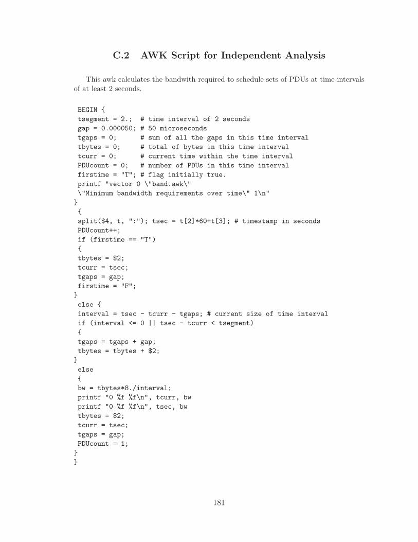
C.2 AWK Script for Independent Analysis
This awk calculates the bandwith required to schedule sets of PDUs at time intervalsof at least 2 seconds.
BEGIN {tsegment = 2.; # time interval of 2 secondsgap = 0.000050; # 50 microsecondstgaps = 0; # sum of all the gaps in this time intervaltbytes = 0; # total of bytes in this time intervaltcurr = 0; # current time within the time intervalPDUcount = 0; # number of PDUs in this time intervalfirstime = "T"; # flag initially true.printf "vector 0 \"band.awk\"\"Minimum bandwidth requirements over time\" 1\n"}{split($4, t, ":"); tsec = t[2]*60+t[3]; # timestamp in secondsPDUcount++;if (firstime == "T"){tbytes = $2;tcurr = tsec;tgaps = gap;firstime = "F";}else {interval = tsec - tcurr - tgaps; # current size of time intervalif (interval <= 0 || tsec - tcurr < tsegment){tgaps = tgaps + gap;tbytes = tbytes + $2;}else{bw = tbytes*8./interval;printf "0 %f %f\n", tcurr, bwprintf "0 %f %f\n", tsec, bwtbytes = $2;tcurr = tsec;tgaps = gap;PDUcount = 1;}}
181
}END {if (interval <= 0){tsec += tsegment;interval = tsec - tcurr - tgaps;}bw = tbytes*8./interval;printf "0 %f %f\n", tcurr, bw;printf "0 %f %f\n", tsec, bw;}
182
APPENDIX D
SIMULATOR SOURCE CODE
183
APPENDIX D
SIMULATOR SOURCE CODE
This appendix contains the source code of the vignette simulator using theOMNeT++ discrete event simulator as the engine, as well as some other auxiliaryprograms used to prepare the input data and extract specific statistics from the simulatoroutput.
//-------------------------------------------------------------------// file: vecstats.cpp//-------------------------------------------------------------------
#include <stdio.h>#include <stdlib.h>#include <float.h>#include <math.h>#define linesize 100
int main(int argc, char *argv[]){FILE *fd;char line[linesize];double min, max, sum, avg1, avg2, std, variance, area,
tInterval, minInterval, maxInterval,t1, t2, mt1, mt2, Mt1, Mt2, val1, val2, time1, time2;
int counter;
min = DBL_MAX;max = 0.;sum = area = 0.;counter = 0;t1 = DBL_MAX;t2 = 0.;maxInterval = 0.;minInterval = DBL_MAX;
if (argc < 2)
184
{printf("Usage: %s <band.vec>\n", argv[0]);return 1;}
if ((fd = fopen(argv[1], "r")) == NULL){printf("Cannot open %s\n", argv[1]);return 2;}
fgets(line, linesize, fd);printf("%s", line);
while (fscanf(fd, " %*d %lf %lf", &time1, &val1) != EOF &&fscanf(fd, " %*d %lf %lf", &time2, &val2) != EOF )
{counter++;if (time1 < t1) t1 = time1;if (time2 > t2) t2 = time2;\
if ((time2 - time1) < minInterval){
minInterval = time2 - time1;mt1 = time1;mt2 = time2;
}if ((time2 - time1) > maxInterval){
maxInterval = time2 - time1;Mt1 = time1;Mt2 = time2;
}if (val1 < min) min = val1;if (val1 > max) max = val1;sum += val1;area += (time2-time1)* (val1+val2)/2.;
}
tInterval = t2 - t1;avg1 = area / tInterval;avg2 = sum / counter;printf("Samples = %d\n", counter);printf("Init time = %11lf\n", t1);printf("Final time = %11lf\n", t2);printf("Min time interval = [ %11lf, %11lf ], length = %lf\n",
185

mt1, mt2, minInterval);printf("Max time interval = [ %11lf, %11lf ], length = %lf\n",
Mt1, Mt2, maxInterval);printf("Minimum bandwidth =%14.1lf\n", min);printf("Maximum bandwidth =%14.1lf\n", max);printf("Point average =%14.1lf\n", avg1);printf("Area average =%14.1lf\n", avg2);
rewind(fd);sum = 0.;fgets(line, linesize, fd);while (fscanf(fd, " %*d %lf %lf", &time1, &val1) != EOF &&
fscanf(fd, " %*d %lf %lf", &time2, &val2) != EOF ){
sum += (val1 - avg2)* (val1 - avg2);}variance = sum / (counter - 1.);std = sqrt(variance);printf("Sample variance =%14.1lf\n", variance);printf("Std deviation =%14.1lf\n", std);}
//-------------------------------------------------------------------// file: pduAnal.c//-------------------------------------------------------------------
/*This program reads in the original PDU log file as well as the PDUsummary file corresponding to a given generator, and produces thefile "extrabyt.txt" that contains pairs of(PDU ID, contribution in bytes of that PDU to the group)*/#include <stdio.h>#include <stdlib.h>#include <string.h>#include <math.h>#include <assert.h>
#define true 1#define false 0#define MAXstring 5000#define MAXpdus 65000#define PDUsimilarity 0.49
int PDUcompareOK (FILE *fd1, FILE *fd2, long int p1, long int p2,
186
int len1, float threshold, int *extraBytes,int *diffLbl);
int readStr(FILE *fd, char a[], char b[], char c[], char d[]);char buffer[MAXstring*4], buffer2[MAXstring*4];char pdu1[MAXstring*4], pdu2[MAXstring*4];char a1[MAXstring], b1[MAXstring], c1[MAXstring], d1[MAXstring];char a2[MAXstring], b2[MAXstring], c2[MAXstring], d2[MAXstring];
// ------------------------------------------------------------------int main(int argc, char *argv[]) {
FILE *fdO1, *fdO2, *fdS, *fdExtraBytes;int moreData = 1, pduCount = 0, blockCount, sameBlock, newBlock,
i, j;int ch, endf, len1, len2, id1, id2, extraBytes, diffLbl,
sumExtraBytes, sumDiffLbl;unsigned int timeStamp1, timeStamp2;long int fpos[MAXpdus], currpos;char a[MAXstring], b[MAXstring], c[MAXstring], d[MAXstring];char type1[50], type2[50];double schedTimeSec1, schedTimeSec2, timeSpan,
hour_equiv = (pow(2.0, 31.0) - 1.0);float threshold = PDUsimilarity;if (argc != 3) {
printf("Usage: %s <file_itsec.data> <file_dataNN.txt>\n",argv[0]);
return 1;}fdO1 = fopen(argv[1], "r"); // Original PDU file (the large one)fdO2 = fopen(argv[1], "r"); // Original PDU file (the large one)
// Same file opened twicefpos[0] = -1;currpos = ftell(fdO1);while ( fgets(buffer, MAXstring*4, fdO1) != NULL ) {
if (buffer[0] == ’<’) fpos[++pduCount] = currpos;currpos = ftell(fdO1);
}// printf ("Number of PDUs in file %s: pduCount=%d\n",// argv[1], pduCount);
// - - - - - - - - - - - - - - - - - - - - - - - - - -fdS = fopen(argv[2], "r"); // Summary file of PDUs.fscanf(fdS, "%x %d %*[^<]%*s %s %*[^:]: %d",
&timeStamp2, &len2, type2, &id2);schedTimeSec2 = (double)(timeStamp2/2) * 3600.0 / hour_equiv;newBlock = true;
187
//To store information about extra bytes.fdExtraBytes = fopen("extrabyt.txt", "w");
while (newBlock) {//newblock = true means not EOF yet and a new empty block is ready.
len1 = len2;id1 = id2;strcpy (type1, type2);blockCount = 1;timeSpan = 0.;sumExtraBytes = 0;schedTimeSec1 = schedTimeSec2;sameBlock = true;do {endf = fscanf(fdS, "%x %d %*[^<]%*s %s %*[^:]: %d",
&timeStamp2, &len2, type2, &id2);if (endf == EOF) {newBlock = false; break;}schedTimeSec2 = (double)(timeStamp2/2) * 3600.0 / hour_equiv;if ( len1 == len2 && strcmp(type1, type2) == 0 &&
PDUcompareOK(fdO1, fdO2, fpos[id1], fpos[id2], len1,threshold, &extraBytes, &diffLbl) ) {
blockCount++;sumDiffLbl += diffLbl;sumExtraBytes += extraBytes;timeSpan = schedTimeSec2 - schedTimeSec1;fprintf(fdExtraBytes, "%d, %d\n", id2, extraBytes);
}else sameBlock = false;
} while (sameBlock);// if sameblock = false then a new block will start// printf("PDUId: %5ld %-12s length: %4d #PDUs: %2d extraBytes: \// %4d diffLabel: %4d timeSpan: %lf\n",// id1, type1, len1, blockCount, sumExtraBytes, sumDiffLbl, timeSpan);// printf("%5d, %-20s, %4d, %2d, %4d, %4d, %lf\n",// id1, type1, len1, blockCount, sumExtraBytes, sumDiffLbl, timeSpan);
}
fclose(fdO1);fclose(fdO2);fclose(fdS);fclose(fdExtraBytes);return 0;
}
// ------------------------------------------------------------------
188
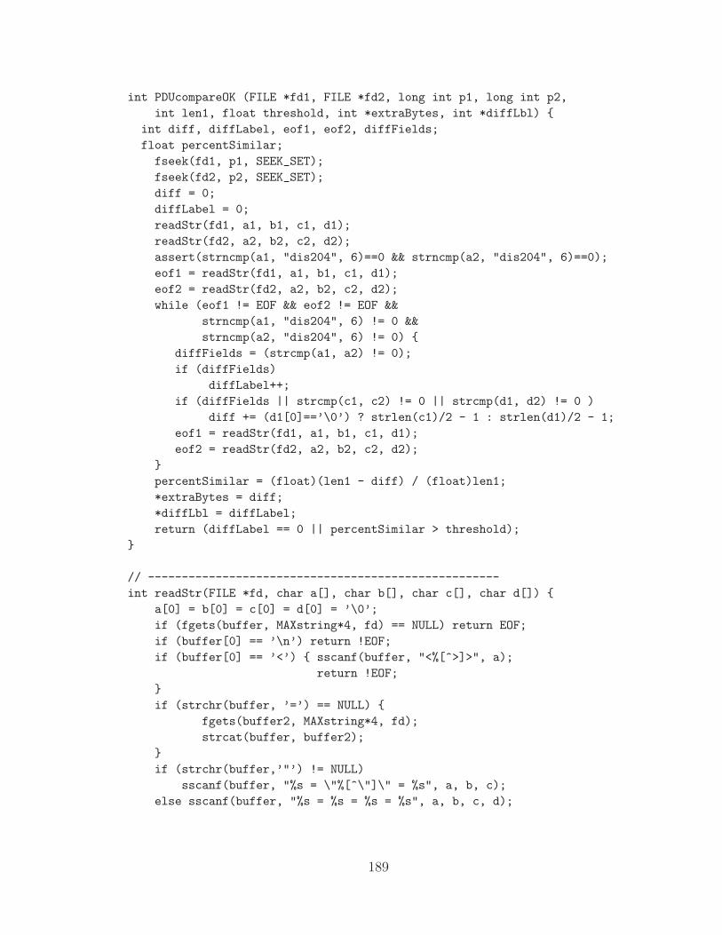
int PDUcompareOK (FILE *fd1, FILE *fd2, long int p1, long int p2,int len1, float threshold, int *extraBytes, int *diffLbl) {
int diff, diffLabel, eof1, eof2, diffFields;float percentSimilar;fseek(fd1, p1, SEEK_SET);fseek(fd2, p2, SEEK_SET);diff = 0;diffLabel = 0;readStr(fd1, a1, b1, c1, d1);readStr(fd2, a2, b2, c2, d2);assert(strncmp(a1, "dis204", 6)==0 && strncmp(a2, "dis204", 6)==0);eof1 = readStr(fd1, a1, b1, c1, d1);eof2 = readStr(fd2, a2, b2, c2, d2);while (eof1 != EOF && eof2 != EOF &&
strncmp(a1, "dis204", 6) != 0 &&strncmp(a2, "dis204", 6) != 0) {
diffFields = (strcmp(a1, a2) != 0);if (diffFields)
diffLabel++;if (diffFields || strcmp(c1, c2) != 0 || strcmp(d1, d2) != 0 )
diff += (d1[0]==’\0’) ? strlen(c1)/2 - 1 : strlen(d1)/2 - 1;eof1 = readStr(fd1, a1, b1, c1, d1);eof2 = readStr(fd2, a2, b2, c2, d2);
}percentSimilar = (float)(len1 - diff) / (float)len1;*extraBytes = diff;*diffLbl = diffLabel;return (diffLabel == 0 || percentSimilar > threshold);
}
// ----------------------------------------------------int readStr(FILE *fd, char a[], char b[], char c[], char d[]) {
a[0] = b[0] = c[0] = d[0] = ’\0’;if (fgets(buffer, MAXstring*4, fd) == NULL) return EOF;if (buffer[0] == ’\n’) return !EOF;if (buffer[0] == ’<’) { sscanf(buffer, "<%[^>]>", a);
return !EOF;}if (strchr(buffer, ’=’) == NULL) {
fgets(buffer2, MAXstring*4, fd);strcat(buffer, buffer2);
}if (strchr(buffer,’"’) != NULL)
sscanf(buffer, "%s = \"%[^\"]\" = %s", a, b, c);else sscanf(buffer, "%s = %s = %s = %s", a, b, c, d);
189
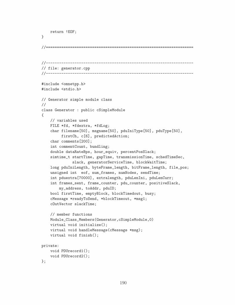
return !EOF;}
//===================================================================
//-------------------------------------------------------------------// file: generator.cpp//-------------------------------------------------------------------
#include <omnetpp.h>#include <stdio.h>
// Generator simple module class//class Generator : public cSimpleModule{
// variables usedFILE *fd, *fdextra, *fdLog;char filename[50], msgname[50], pduIniType[50], pduType[50],
firstCh, c[6], predictedAction;char comments[200];int commentCount, bundling;double dataRateBps, hour_equiv, percentPosSlack;simtime_t startTime, gapTime, transmissionTime, schedTimeSec,
slack, generatorServiceTime, blockWaitTime;long pduIniLength, byteFrame_length, bitFrame_length, file_pos;unsigned int eof, num_frames, numNodes, sendTime;int pduextra[70000], extralength, pduLenIni, pduLenCurr;int frames_sent, frame_counter, pdu_counter, positiveSlack,
my_address, toAddr, pduID;bool firstTime, emptyBlock, blockTimedout, busy;cMessage *readyToSend, *blockTimeout, *msg1;cOutVector slackTime;
// member functionsModule_Class_Members(Generator,cSimpleModule,0)virtual void initialize();virtual void handleMessage(cMessage *msg);virtual void finish();
private:void PDUrecord1();void PDUrecord2();
};
190
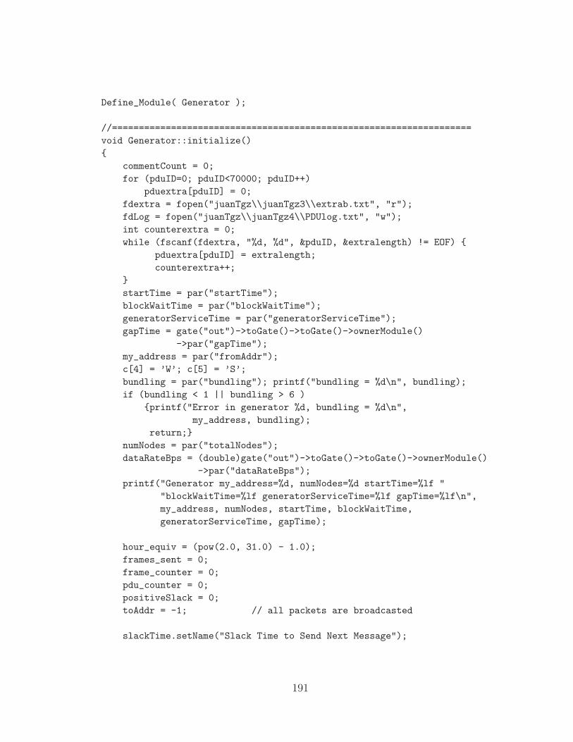
Define_Module( Generator );
//===================================================================void Generator::initialize(){
commentCount = 0;for (pduID=0; pduID<70000; pduID++)
pduextra[pduID] = 0;fdextra = fopen("juanTgz\\juanTgz3\\extrab.txt", "r");fdLog = fopen("juanTgz\\juanTgz4\\PDUlog.txt", "w");int counterextra = 0;while (fscanf(fdextra, "%d, %d", &pduID, &extralength) != EOF) {
pduextra[pduID] = extralength;counterextra++;
}startTime = par("startTime");blockWaitTime = par("blockWaitTime");generatorServiceTime = par("generatorServiceTime");gapTime = gate("out")->toGate()->toGate()->ownerModule()
->par("gapTime");my_address = par("fromAddr");c[4] = ’W’; c[5] = ’S’;bundling = par("bundling"); printf("bundling = %d\n", bundling);if (bundling < 1 || bundling > 6 )
{printf("Error in generator %d, bundling = %d\n",my_address, bundling);
return;}numNodes = par("totalNodes");dataRateBps = (double)gate("out")->toGate()->toGate()->ownerModule()
->par("dataRateBps");printf("Generator my_address=%d, numNodes=%d startTime=%lf "
"blockWaitTime=%lf generatorServiceTime=%lf gapTime=%lf\n",my_address, numNodes, startTime, blockWaitTime,generatorServiceTime, gapTime);
hour_equiv = (pow(2.0, 31.0) - 1.0);frames_sent = 0;frame_counter = 0;pdu_counter = 0;positiveSlack = 0;toAddr = -1; // all packets are broadcasted
slackTime.setName("Slack Time to Send Next Message");
191
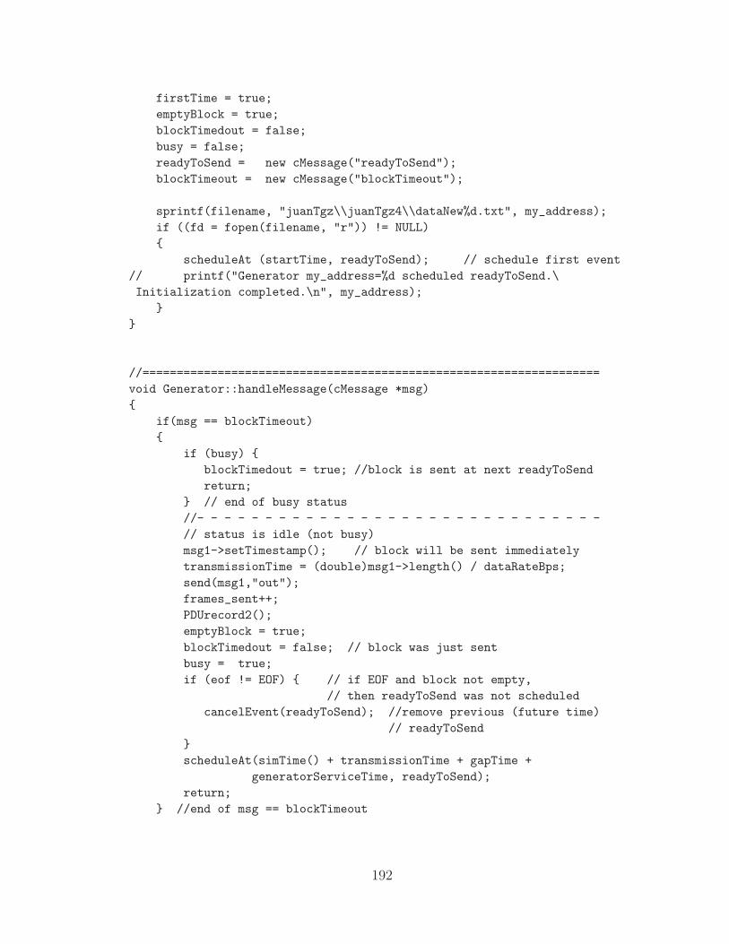
firstTime = true;emptyBlock = true;blockTimedout = false;busy = false;readyToSend = new cMessage("readyToSend");blockTimeout = new cMessage("blockTimeout");
sprintf(filename, "juanTgz\\juanTgz4\\dataNew%d.txt", my_address);if ((fd = fopen(filename, "r")) != NULL){
scheduleAt (startTime, readyToSend); // schedule first event// printf("Generator my_address=%d scheduled readyToSend.\Initialization completed.\n", my_address);
}}
//===================================================================void Generator::handleMessage(cMessage *msg){
if(msg == blockTimeout){
if (busy) {blockTimedout = true; //block is sent at next readyToSendreturn;
} // end of busy status//- - - - - - - - - - - - - - - - - - - - - - - - - - - - - -// status is idle (not busy)msg1->setTimestamp(); // block will be sent immediatelytransmissionTime = (double)msg1->length() / dataRateBps;send(msg1,"out");frames_sent++;PDUrecord2();emptyBlock = true;blockTimedout = false; // block was just sentbusy = true;if (eof != EOF) { // if EOF and block not empty,
// then readyToSend was not scheduledcancelEvent(readyToSend); //remove previous (future time)
// readyToSend}scheduleAt(simTime() + transmissionTime + gapTime +
generatorServiceTime, readyToSend);return;
} //end of msg == blockTimeout
192

//- - - - - - - - - - - - - - - - - - - - - - - - - - - - - - - - - -
// msg is not blockTimeout, should be readyToSendif (msg == readyToSend){
if (blockTimedout) { //current block has priority over new PDUsmsg1->setTimestamp(); // block will be sent immediatelytransmissionTime = (double)msg1->length() / dataRateBps;send(msg1,"out");frames_sent++;PDUrecord2();emptyBlock = true;blockTimedout = false; // block was just sentbusy = true;scheduleAt(simTime() + transmissionTime + gapTime +
generatorServiceTime, readyToSend);return;
} //end of blockTimedout//- - - - - - - - - - - - - - - - - - - - - - - - - - - - - - - - - -
// msg is readyToSend & not blockTimedoutfirstCh = getc(fd); //skips over comments indicated by
// ’%’ in first charwhile (firstCh == ’#’) {
fgets(comments, 200, fd);commentCount++;printf("Comments # %d in %s are: %s\n",
commentCount, filename, comments);firstCh = getc(fd);
}ungetc(firstCh, fd);file_pos = ftell(fd);eof = fscanf(fd,
"%x %ld | %*s %*d <dis204 %s PDU>: %d %c %c %c %c",&sendTime, &byteFrame_length, pduType, &pduID,&c[0],&c[1],&c[2],&c[3]);
// c[0] is neural network (column 1)// c[1] is type (column 2)// c[2] is type and length (column 3)// c[3] is type, length and timestamp (column 4)// c[4] = W always wait// c[5] = S always send
predictedAction = c[bundling-1];if (eof == EOF) {
if (emptyBlock) { // end of generator simulation
193

percentPosSlack = (double)positiveSlack *100.0 / (double)pdu_counter;
printf("EOF in file %11s at time %lf, positive slack ""frames=%6d(%5.2lf%%), total PDUs=%6d, total frames"" built=%6d, total frames sent=%6d\n",filename, simTime(), positiveSlack, percentPosSlack,pdu_counter, frame_counter, frames_sent);fclose(fdLog);
} // end of emptyBlockelse { // block is not empty
busy = false;cancelEvent(blockTimeout);scheduleAt(simTime(), blockTimeout);
}return;
} // end eof == EOF// - - - - - - - - - - - - - - - - - - - - - - - - - - - - - - - - -
// msg = readyToSend & not blockTimedout & not EOF// we read a new PDU from the summary file.
//conversion from OTB units to secondsschedTimeSec = (double)(sendTime/2) * 3600.0 / hour_equiv;bitFrame_length = byteFrame_length * 8;slack = schedTimeSec - simTime();if (firstTime) { // first time this particular PDU
// was read from the input file.pdu_counter++;slackTime.record(slack);if (slack >= 0) positiveSlack++;firstTime = false; // this particular PDU
//won’t be recorded again.}if (slack > 0.) {
busy = false; // we will be idle for a whileif (fseek(fd, file_pos, SEEK_SET)) perror( "Fseek failed" );// next packet is scheduled at timestamp in PDUscheduleAt(schedTimeSec, readyToSend);return;
} // end of slack > 0.// - - - - - - - - - - - - - - - - - - - - - - - - - - - - - - - - - -
// msg = readyToSend & not blockTimedout & not EOF & slack <= 0.// This PDU must be grouped for replication
firstTime = true; // to record slack for next PDU.if (emptyBlock) { //This PDU will be the first in the new block
194
sprintf(msgname,"Data%d F%d T%d",++frame_counter, my_address, toAddr);
msg1 = new cMessage(msgname);msg1->setLength(bitFrame_length);PDUrecord1();strcpy(pduIniType,pduType);pduIniLength = byteFrame_length;if (predictedAction == ’s’ || predictedAction == ’S’){ // predicted action = send
msg1->setTimestamp();transmissionTime = (double)msg1->length() / dataRateBps;send(msg1,"out");frames_sent++;PDUrecord2();busy = true;scheduleAt(simTime() + transmissionTime + gapTime +
generatorServiceTime, readyToSend);}else { // predicted action = wait
scheduleAt(simTime() + blockWaitTime, blockTimeout);busy = false;emptyBlock = false;scheduleAt(simTime() + generatorServiceTime, readyToSend);
}return;
} // end of emptyBlock// - - - - - - - - - - - - - - - - - - - - - - - - - - - - - - - - -
// msg = readyToSend & not blockTimedout &// not EOF & slack <= 0. & not emptyBlock
if ((strcmp(pduIniType,pduType)==0) &&(pduIniLength==byteFrame_length)) { //compatible PDU
//grouping (bundling)msg1->setLength(msg1->length()+(pduextra[pduID]*8));PDUrecord1();if (predictedAction == ’s’ || predictedAction == ’S’) {
msg1->setTimestamp(); // predicted action = sendtransmissionTime = (double)msg1->length() / dataRateBps;send(msg1,"out");frames_sent++;PDUrecord2();cancelEvent(blockTimeout);emptyBlock = true;busy = true;scheduleAt(simTime() + transmissionTime + gapTime +
195

generatorServiceTime, readyToSend);} // end of predictedAction = sendelse { // predicted action = wait
busy = true;scheduleAt(simTime() + generatorServiceTime, readyToSend);
} // end of predicted action = waitreturn;
} // end of compatible PDU// - - - - - - - - - - - - - - - - - - - - - - - - - - - - - - - - -
// msg = readyToSend & not blockTimedout &// not EOF & slack <= 0. & not emptyBlock & PDU not compatible
msg1->setTimestamp();transmissionTime = (double)msg1->length() / dataRateBps;send(msg1,"out");frames_sent++;PDUrecord2();cancelEvent(blockTimeout);sprintf(msgname,"Data%d F%d T%d",++frame_counter, my_address, toAddr);msg1 = new cMessage(msgname);msg1->setLength(bitFrame_length);PDUrecord1();strcpy(pduIniType,pduType);pduIniLength = byteFrame_length;if (predictedAction == ’s’ || predictedAction == ’S’){ // predicted action = send
// this 1-PDU block is considered to have timedoutblockTimedout = true;
}else { // predicted action = wait
scheduleAt(simTime() + blockWaitTime +generatorServiceTime, blockTimeout);
} // end of predicted action = waitbusy = true;scheduleAt(simTime() + transmissionTime + gapTime +
generatorServiceTime, readyToSend);return; // msg = readyToSend & not EOF & slack <= 0.
} // end msg == readyToSend//- - - - - - - - - - - - - - - - - - - - - - - - - - - - - -
printf("Generator %d: Unrecognized message\n", my_address);return;
}
196
//===================================================================void Generator::finish() {
ev << "Generator " << my_address << ": No of frames sent = "<< frame_counter << endl;
}
//===================================================================void Generator::PDUrecord1() {
if (my_address == 24) fprintf(fdLog, "%d ", pduID);}
//===================================================================void Generator::PDUrecord2() {
double t, seconds;int minutes;t = simTime();minutes = (int) t/60.;seconds = t - minutes*60.;
if (my_address == 24) {double t, seconds;int minutes;t = simTime();minutes = (int) (t/60.);seconds = t - minutes*60.;fprintf(fdLog, ": %lf (:%d:%.3lf) | \tframes:%d\n",
t, minutes, seconds, frames_sent);}
}
//-------------------------------------------------------------// file: sink.cpp//-------------------------------------------------------------
#include <omnetpp.h>
//// Sink simple module class//class Sink : public cSimpleModule{
int my_address, from, to, collisionCounter, framesReceived,unrecognized, wrongAddress;
double travelTime;
197
cMessage *collision;char *p;
// member functionsModule_Class_Members(Sink,cSimpleModule,0)virtual void initialize();virtual void handleMessage(cMessage *msg);virtual void finish();
cDoubleHistogram *travelDist;cOutVector travelHist;cStdDev travelStats;
cOutVector collHistAccum;
};
Define_Module( Sink );
void Sink::initialize(){
collisionCounter = 0;my_address = parentModule()->par("nodeID");collision = new cMessage("collision");travelDist = new cDoubleHistogram(
"Travel Time Distribution at destination", 100);travelDist->setRange(0, 100);travelHist.setName("Travel Time History");travelStats.setName("travel Stats");collHistAccum.setName("Collision Accumulation");framesReceived = 0;unrecognized = 0;wrongAddress = 0;
}
void Sink::handleMessage(cMessage *msg){
// msg == collisionif (strcmp(msg->name(), collision->name()) == 0){
collisionCounter++;collHistAccum.record (collisionCounter);delete msg;return;
}
198
p = strchr(msg->name(),’F’);
if (p == NULL){ ev<<"Sink["<<my_address<<"] unrecognized deleted "
<<msg->name()<<endl;delete msg; // unrecognized message, considered an errorunrecognized++;
}else // p != NULL, this is a regular messagesscanf(p, "F%d T%d", &from, &to);
if (to == -1 || to == my_address){
// ev << "Sink[" << my_address << "] Frame " << msg->name()<<" at T = " << simTime() << endl;
travelTime = simTime() - msg->timestamp();// travel time travelStatsistics collectiontravelDist->collect (travelTime);travelHist.record(travelTime);travelStats.collect(travelTime);framesReceived++;
}else wrongAddress++;
delete msg;}
void Sink::finish(){
long num_samples;double smallest, largest, mean,
standard_deviation, variance;
ev << endl << endl<< "*** Module: " << fullPath() << "***" << endl;ev << "Total arrivals: " << travelDist->samples() << endl;ev << "Estimation of the travel stationary \distribution of travel time.\n";ev << "Travel time, # of messages, estimated \probability density function.\n";for(int i=0; i<travelDist->cells(); ++i){ if(travelDist->cell(i) > 0)
{ ev << i << ":\t" << travelDist->cell(i);ev << "\t" << travelDist->cellPDF(i) << endl;
}
199

}recordStats("Travel Time Distribution Statistics", travelDist);ev << "Travel Time Statistics" << endl;num_samples = travelStats.samples();smallest = travelStats.min();largest = travelStats.max();mean = travelStats.mean();standard_deviation = travelStats.stddev(),variance = travelStats.variance();ev << "Number of samples: " << num_samples << endl;ev << "Smallest time: " << smallest << endl;ev << "Largest time: " << largest << endl;ev << "Mean value: " << mean << endl;ev << "Standard Dev: " << standard_deviation << endl;ev << "Variance: " << variance << endl;printf("Sink %d: Total frames received=%d, total collisions \detected=%d total unrecognized=%d wrong address=%d\n",
my_address, framesReceived, collisionCounter,unrecognized, wrongAddress);
}
//-------------------------------------------------------------// file: router.cpp//-------------------------------------------------------------
#include <omnetpp.h>#include <string.h>
//// Router simple module class//class Router : public cSimpleModule{
int routerID, nodesPerPlane, totalNodes;int inf, sup;int from, to, inGate, outGate;// 3 communication channels.int collisionCount[3], collisionCountNonReset[3];double startTime, routerServiceTime, transmissionTime,
collInterval, gapTime[4], dataRate[4];int fromLan, toLan, fromSP, toSP, fromPP, toPP; // frame counters
cQueue queue;cMessage *sendNow, *readyToSend, *collision,
*collStatsNow, *msg1, *msg2;
200
cDoubleHistogram *jobDist;cOutVector jobsInSys;cStdDev stat;
cDoubleHistogram *collDist[3];cOutVector collInSys[3];
cOutVector collHistAccum;
// member functionsModule_Class_Members (Router, cSimpleModule,0)virtual void initialize ();virtual void finish ();virtual void handleMessage (cMessage *msg);void serveMessage();int outputGate (int inGate, int from, int to);
};
Define_Module( Router );
//=============================================================void Router::initialize(){
int i;startTime = par("startTime");routerID = par("routerID");nodesPerPlane = par("nodesPerPlane");totalNodes = par("totalNodes");routerServiceTime = par("routerServiceTime");
gapTime[0] = gate("outToLocal")->toGate()->ownerModule()->par("gapTime");
gapTime[1] = gate("outToWirelessPP")->toGate()->toGate()->ownerModule()->par("gapTime");
gapTime[2] = gate("outToWirelessSP")->toGate()->toGate()->ownerModule()->par("gapTime");
gapTime[3] = gapTime[1] > gapTime[2] ? gapTime[1] : gapTime[2];
dataRate[0] = (double)gate("outToLocal") ->toGate()->ownerModule()->par("dataRateBps");
dataRate[1] = (double)gate("outToWirelessPP")->toGate()->toGate()->ownerModule()->par("dataRateBps");
201
dataRate[2] = (double)gate("outToWirelessSP")->toGate()->toGate()->ownerModule()->par("dataRateBps");
dataRate[3] = dataRate[1] < dataRate[2] ? dataRate[1] : dataRate[2];
collision = new cMessage("collision");collStatsNow = new cMessage("collStatsNow");readyToSend = new cMessage("readyToSend");sendNow = new cMessage("sendNow");
inf = nodesPerPlane * routerID;sup = inf + nodesPerPlane - 1;// msg1 = NULL because initial state is "readyToSend"msg1 = NULL;
jobDist = new cDoubleHistogram("Queue Message Distribution (router)", 100);
jobDist->setRange(0, 100);jobsInSys.setName("Messages in System (router)");stat.setName("stat");
{ char *titles[3] = { "Collisions at inFromLocal (Ethernet)","Collisions at inFromWirelessPP","Collisions at inFromWirelessSP" };
for (i = 0; i<3; i++){ collisionCount[i] = 0;
collisionCountNonReset[i] = 0;collDist[i] = new cDoubleHistogram(titles[i], 100);collDist[i]->setRange(0, 100);collInSys[i].setName(titles[i]);
}}collHistAccum.setName("Collision Accumulation");
// count collisions in 1-second intervalscollInterval = 1.;// frame counters set to 0fromLan = toLan = fromSP = toSP = fromPP = toPP = 0;// first event to request collision statistics.scheduleAt(collInterval+startTime, collStatsNow);
}
//=================================================================void Router::handleMessage(cMessage *msg){
202
if (strcmp(msg->name(), collision->name()) == 0) // msg == collision{ inGate = msg->arrivalGate()->id() /2; // inGate = 0 or 1 or 2
collisionCount[inGate]++;collisionCountNonReset[inGate]++;collHistAccum.record (collisionCountNonReset[0] +
collisionCountNonReset[1] +collisionCountNonReset[2]);
delete msg;return;
}
//- - - - - - - - - - - - - - - - - - - - - - - - - - - - - - - - -// Statistics collection requested nowelse if (msg == collStatsNow){ for (int i=0; i<3; i++)
{ collDist[i]->collect (collisionCount[i]);collInSys[i].record(collisionCount[i]);
// starts a new count for the next intervalcollisionCount[i] = 0;
}scheduleAt(simTime()+collInterval, collStatsNow);return;
}
//- - - - - - - - - - - - - - - - - - - - - - - - - - - - - - -else if (msg == sendNow){
switch (outGate){
case 0:send(msg1, "outToLocal");toLan++;break;
case 1:send(msg1, "outToWirelessPP");toPP++;break;
case 2:send(msg1, "outToWirelessSP");toSP++;break;
case 3:
203
msg2 = (cMessage *) msg1->dup();send(msg1, "outToWirelessPP");toPP++;send(msg2, "outToWirelessSP");toSP++;break;
}}
//- - - - - - - - - - - - - - - - - - - - - - - - - - - - - - -else if (msg == readyToSend) // last gapTime has elapsed{
if ( queue.empty() ) // There are no remaining messages in queue{
msg1 = NULL;}
else{
msg1 = (cMessage *) queue.pop();// schedules a sendNow and readyToSend for msg1
serveMessage();}
}
//- - - - - - - - - - - - - - - - - - - - - - - - - - - - - - -else // msg == regular message || unrecognized{
// to ignore messages sent to satellite from other planeschar *p = strchr(msg->name(),’F’);sscanf(p, "F%d T%d", &from, &to);inGate = msg->arrivalGate()->id();
// gate #4: inFromWirelessSPif ((inGate == 4) && (from != totalNodes)){
delete msg;return;
}
// msg arrived while server is idle, current state is "readyToSend"if (msg1 == NULL)
// Statistics collection: queue length was 0{ jobDist->collect(0);
jobsInSys.record(0);stat.collect(0.);
204
msg1 = msg; //msg will be serviced immediatelyserveMessage(); //schedules a sendNow and readyToSend for msg1
}
else // Arrival while server is busy{
// n msgs in queue + 1 being servicedjobDist->collect(queue.length()+1);jobsInSys.record(queue.length()+1);stat.collect(queue.length()+1.);queue.insert( msg );
}} // end of regular message
} // end handleMessage
//===========================================================void Router::serveMessage(){
char *p = strchr(msg1->name(),’F’);if (p == NULL) // unrecognized message, considered an error{
ev<<"Router["<<routerID<<"] unrecognized deleted "<<msg1->name()<<endl;
delete msg1;scheduleAt( simTime(), readyToSend );return;
}
sscanf(p, "F%d T%d", &from, &to);// inGate: 0/2 = 0, 2/2 = 1 or 4/2 = 2
inGate = (msg1->arrivalGate()->id()) / 2;if (inGate==0)fromLan++;if (inGate==1)fromPP++;if (inGate==2)fromSP++;
// outGate = -1, 0, 1, 2, 3outGate = outputGate(inGate, from, to);if (outGate < 0){
delete msg1;scheduleAt( simTime(), readyToSend );return;
}
205
transmissionTime = msg1->length() / dataRate[outGate];scheduleAt( simTime() + routerServiceTime, sendNow );scheduleAt( simTime() + routerServiceTime + transmissionTime
+ gapTime[outGate], readyToSend );
}
//========================================================int Router::outputGate(int inGate, int from, int to){
switch (inGate){
case 0: // inFromLocalif (to == -1) return 3; // outToWirelessSP
// and outToWirelessPPif (to == totalNodes) return 2; // outToWirelessSPif (to < inf || to > sup) return 1; // outToWirelessPPreturn -1; // delete messagebreak;
case 1: // inFromWirelessPPif (to == -1) return 0; // outToLocal
// delete, this case shoud not occurif (to == totalNodes) return -1;if (inf <= to && to <= sup) return 0; // outToLocalreturn -1; // delete messagebreak;
case 2: // inFromWirelessSPif (
(from == totalNodes) &&((to == -1) || (inf <= to && to <= sup))
// from satellite (groundStation) to local broadcast) return 0;
return -1; // delete messagebreak;
}return -2; // unreachable code to eliminate C++ warning.
}
//=======================================================void Router::finish(){
206
long num_samples;double smallest, largest, mean, standard_deviation, variance;
ev << endl << endl<< "*** Module: " << fullPath() << "***" << endl;ev << "Total arrivals:\t" << jobDist->samples() << endl;ev << "Total collisions detected:"<<endl;ev << "At inFromLocal: " << collisionCountNonReset[0]<<endl;ev << "At wirelessPP: " << collisionCountNonReset[1]<<endl;ev << "At wirelessSP: " << collisionCountNonReset[2]<<endl<<endl;
ev << "Estimation of the stationary distribution of messages \as observed by an arrival.\n";ev << "Queue length, # arrivals that saw n messages in queue, \estimated probability density function.\n";for(int i=0; i<jobDist->cells(); ++i){ if(jobDist->cell(i) > 0)
{ ev << i << ":\t" << jobDist->cell(i);ev << "\t" << jobDist->cellPDF(i) << endl;
}}recordStats("Message Distribution Statistics", jobDist);ev << "Queue length statistics" << endl;num_samples = stat.samples();smallest = stat.min();largest = stat.max();mean = stat.mean();standard_deviation = stat.stddev(),variance = stat.variance();ev << "Number of samples: " << num_samples << endl;ev << "Smallest queue: " << smallest << endl;ev << "Largest queue: " << largest << endl;ev << "Mean value: " << mean << endl;ev << "Standar Dev: " << standard_deviation << endl;ev << "Variance: " << variance << endl;printf("Router %d: frames fromLan=%d, toLan=%d, fromSP=%d, \toSP=%d, fromPP=%d, toPP=%d, in queue=%d\n",routerID, fromLan, toLan, fromSP, toSP, fromPP,toPP, queue.length());
}
//-------------------------------------------------------------// file: satellite.cpp//-------------------------------------------------------------
#include <omnetpp.h>
207
#include <string.h>
//// Satellite simple module class//class Satellite : public cSimpleModule{
// arrays are of length 2 because of the 2 communication channels.int satelliteID, totalNodes;double startTime, satServiceTime, transmissionTime,
gapTime[2], dataRate[2];double WSPposition, WGSposition, collInterval;int from, to, inGate, outGate, numGate;int collisionCount[2], collisionCountNonReset[2], byteCount,
framesToGS, framesToPlanes, framesReceivedFromGS,framesReceivedFromSP, unrecognized;
char *p;
cQueue queue;cMessage *sendNow, *readyToSend, *collision, *collStatsNow, *msg1;cDoubleHistogram *jobDist, *byteDist;cOutVector jobsInSys, bytesInSys;cStdDev msgStat, byteStat;cDoubleHistogram *collDist[2];cOutVector collInSys[2];
// member functionsModule_Class_Members(Satellite, cSimpleModule,0)virtual void initialize();virtual void finish();virtual void handleMessage(cMessage *msg);void serveMessage();int outputGate (int inGate, int from, int to);
};
Define_Module( Satellite );
//===============================================================void Satellite::initialize(){
int i;startTime = par("startTime");satServiceTime = par("satServiceTime");
208
sendNow = new cMessage("sendNow");collision = new cMessage("collision");collStatsNow = new cMessage("collStatsNow");readyToSend = new cMessage("readyToSend");
gapTime[0] = gate("outBus1")->toGate()->ownerModule()->par("gapTime");
gapTime[1] = gate("outBus2")->toGate()->ownerModule()->par("gapTime");
dataRate[0] = (double)gate("outBus1")->toGate()->ownerModule()->par("dataRateBps");
dataRate[1] = (double)gate("outBus2")->toGate()->ownerModule()->par("dataRateBps");
satelliteID = par("satelliteID");// totalNodes = 3*8 = 24, but 0,...,24 = 25 nodes
totalNodes = par("totalNodes");// WSPposition = par("WSPposition");// WGSposition = par("WGSposition");
msg1 = NULL;
jobDist = new cDoubleHistogram("Queue Message Distribution (satellite)", 100);
jobDist->setRange(0, 100);jobsInSys.setName("Messages in System (satellite)");byteDist = new cDoubleHistogram(
"Queue Byte Distribution (satellite)", 100);byteDist->setRange(0, 100);bytesInSys.setName("Bytes in System (satellite)");
{ char *titles[2] = { "Collisions at wirelessGS","Collisions at wirelessSP" };
for (i = 0; i<2; i++){ collisionCount[i] = 0;
collisionCountNonReset[i] = 0;collDist[i] = new cDoubleHistogram(titles[i], 100);collDist[i]->setRange(0, 100);collInSys[i].setName(titles[i]);
}}framesToGS = 0; // to count frames sent to Ground StationframesToPlanes = 0;framesReceivedFromGS = 0;
209

framesReceivedFromSP = 0;unrecognized = 0;byteCount = 0; // counts bytes in queue.collInterval = 1.; // count collisions in 1-second intervals
// first event to request collision statistics.scheduleAt(collInterval+startTime, collStatsNow);
}
//==============================================================void Satellite::handleMessage(cMessage *msg){
if (strcmp(msg->name(), collision->name()) == 0) //msg == collision{
inGate = msg->arrivalGate()->id() /2; //inGate = 0 or 1collisionCount[inGate]++;collisionCountNonReset[inGate]++;delete msg;return;
}
//- - - - - - - - - - - - - - - - - - - - - - - - - - - - - - - -else if (msg == collStatsNow) // Statistics collection requested now{ for (int i=0; i<2; i++)
{ collDist[i]->collect (collisionCount[i]);collInSys[i].record(collisionCount[i]);
// starts a new count for the next intervalcollisionCount[i] = 0;
}scheduleAt(simTime()+collInterval, collStatsNow);return;
}
//- - - - - - - - - - - - - - - - - - - - - - - - - - - - - - -else if (msg == sendNow){
switch (outGate){
case 0:send(msg1, "outBus1"); // wirelessGSframesToGS++;break;
case 1:send(msg1, "outBus2"); // wirelessSP
210
framesToPlanes++;break;
}}
//- - - - - - - - - - - - - - - - - - - - - - - - - - - - - - -else if (msg == readyToSend) // last gapTime has elapsed{
if ( queue.empty() ) // There are no remaining messages in queue{
msg1 = NULL;if (byteCount != 0)printf("Satellite: Error, empty queue has byteCount = %d\n",
byteCount);}
else{
msg1 = (cMessage *) queue.pop();// subtracts # bytes taken from the queue
byteCount -= msg1->length()/8;// schedules a sendNow and readyToSend for msg1
serveMessage();}
}
//- - - - - - - - - - - - - - - - - - - - - - - - - - - - -else // msg == regular message or unrecognized{
// msg arrived while server is idle, current state is "readyToSend"if (msg1 == NULL){
// Statistics collection: queue length was 0jobDist->collect(0);jobsInSys.record(0);msgStat.collect(0.);
// Statistics collection: queue length was 0byteDist->collect(0);bytesInSys.record(0);byteStat.collect(0.);msg1 = msg; // msg will be serviced immediately
// schedules a sendNow and readyToSend for msg1serveMessage();
}else // Arrival while server is busy
211
{// n msgs in queue + 1 being serviced
jobDist->collect(queue.length()+1);jobsInSys.record(queue.length()+1);msgStat.collect(queue.length()+1.);
// accumulates # bytes in new messagebyteCount += msg->length()/8;
// n msgs in queue + 1 being servicedbyteDist->collect(byteCount);bytesInSys.record(byteCount);byteStat.collect(byteCount);queue.insert( msg );
}} // end of regular message
} // end handleMessage
//===========================================================void Satellite::serveMessage(){
char *p = strchr(msg1->name(),’F’);if (p == NULL) // unrecognized message, considered an error{
ev<<"Satellite: unrecognized message deleted "<<endl;delete msg1;unrecognized++;scheduleAt( simTime(), readyToSend );return;
}
sscanf(p, "F%d T%d", &from, &to);inGate = (msg1->arrivalGate()->id()) / 2; //inGate: 0/2=0, 2/2=1if (inGate==0) framesReceivedFromGS++;else framesReceivedFromSP++;outGate = outputGate(inGate, from, to); // outGate = -1, 0, 1if (outGate < 0){
delete msg1;unrecognized++;scheduleAt( simTime(), readyToSend );return;
}
transmissionTime = msg1->length() / dataRate[outGate];
212
scheduleAt( simTime() + satServiceTime, sendNow );scheduleAt( simTime() + satServiceTime + transmissionTime +
gapTime[outGate], readyToSend );
}
//============================================================int Satellite::outputGate(int inGate, int from, int to){
switch (inGate){
case 0: // inBus1 (wirelessGS)if (to < totalNodes) return 1; // WirelessSPreturn -1; // delete messagebreak;
case 1: // inBus2 (wirelessSP)if (to == -1 || to == totalNodes)
return 0; // inBus1 wirelessGSreturn -1; // delete messagebreak;
}
return -2; // unreachable code to eliminate C++ warning.}
//=======================================================void Satellite::finish(){
long num_samples;double smallest, largest, mean, standard_deviation, variance;
ev << endl << endl<< "*** Module: " << fullPath()<< "***" << endl;
ev << "Total arrivals:\t" << jobDist->samples() << endl;ev << "Total collisions detected:"<<endl;ev << "At wirelessGS: " << collisionCountNonReset[0]
<<endl;ev << "At wirelessSP: " << collisionCountNonReset[1]
<<endl<<endl;ev << "Estimation of the stationary distribution of \messages as observed by an arrival.\n";ev << "Queue length, # arrivals that saw n messages in \
213

queue, estimated probability density function.\n";for(int i=0; i<jobDist->cells(); ++i){ if(jobDist->cell(i) > 0)
{ ev << i << ":\t" << jobDist->cell(i);ev << "\t" << jobDist->cellPDF(i) << endl;
}}recordStats("Message Distribution Statistics", jobDist);ev << "Queue length statistics" << endl;num_samples = msgStat.samples();smallest = msgStat.min();largest = msgStat.max();mean = msgStat.mean();standard_deviation = msgStat.stddev(),variance = msgStat.variance();ev << "Number of samples: " << num_samples << endl;ev << "Smallest queue: " << smallest << endl;ev << "Largest queue: " << largest << endl;ev << "Mean value: " << mean << endl;ev << "Standar Dev: " << standard_deviation << endl;ev << "Variance: " << variance << endl;printf("Satellite: total frames received from GS=%d, \sent to SP=%d\n",
framesReceivedFromGS, framesToPlanes);printf("Satellite: received from SP=%d, sent to GS=%d, \unrecognized=%d, in queue=%d\n",framesReceivedFromSP, framesToGS, unrecognized, queue.length());
}
//-------------------------------------------------------------// File: simplebus.cc// Based on an example by Andras Varga, author of OMNeT++.//-------------------------------------------------------------
#include <assert.h>#include <omnetpp.h>
#define MAX_NUM_TAPS 50
class SimpleBus : public cSimpleModule{
struct sTransmission{
int tap, channel;
214

bool upstream;bool isCollision;simtime_t busyStart, busyEnd;cMessage *endEvent;cMessage *frame;
};
int prueba;Module_Class_Members(SimpleBus,cSimpleModule,0);virtual void initialize();virtual void handleMessage(cMessage *msg);
cMessage *createMessage();sTransmission *createTransmission();void recycleMessage(cMessage *msg);void recycleTransmission(sTransmission *tr);
private:int numTaps;int numChannels;
bool wantCollisionModeling;bool wantCollisionSignal;bool isFullDuplex;double delaySecPerMeter;double dataRateBps;
char busTypePosition[20];double tapPositions[MAX_NUM_TAPS];cArray tapStates;
cHead recycledMessages;cLinkedList recycledTransmissions;
};
Define_Module(SimpleBus);
void SimpleBus::initialize(){
// get parameters// collision modeling flag
wantCollisionModeling = par("wantCollisionModeling");// "send collision signals" flag
wantCollisionSignal = par("wantCollisionSignal");
215
// number of independent channelsnumChannels = par("numChannels");
// channel modeisFullDuplex = par("isFullDuplex");
// delay of the busdelaySecPerMeter = par("delaySecPerMeter");
// data rate of the busdataRateBps = par("dataRateBps");strcpy(busTypePosition, par("busType").stringValue());strcat(busTypePosition, "position");
// busTypePosition = LANposition, WPPposition, WSPposition,// or WGSposition
// query the number of taps and the their positions (in meters)numTaps = gate("out")->size();assert(numTaps < MAX_NUM_TAPS);for (int k=0; k<numTaps; k++){
tapPositions[k] = gate("out",k)->toGate()->ownerModule()->par(busTypePosition);
}
// create linked lists that will hold channel states at taps// (sTransmission structs)tapStates.setName("tapStates");for (int i=0; i<numTaps; i++){
for (int j=0; j<numChannels; j++){
char listname[64];sprintf(listname,"tap%dchannel%d",i,j);cLinkedList *list = new cLinkedList(listname);tapStates.addAt(i*numChannels+j, list);
}}
recycledMessages.setName("recycledMessages");recycledTransmissions.setName("recycledTransmissions");
}
cMessage *SimpleBus::createMessage(){
return new cMessage;}
216

SimpleBus::sTransmission *SimpleBus::createTransmission(){
return new sTransmission;}
void SimpleBus::recycleMessage(cMessage *msg){
delete msg;}
void SimpleBus::recycleTransmission(sTransmission *tr){
delete tr;}
void SimpleBus::handleMessage(cMessage *msg){
cMessage *msg_new;
// is msg a frame to be transmitted on the bus?if (!msg->isSelfMessage()){
// get position where packet dropped indouble packetPos = tapPositions[msg->arrivalGate()->index()];
// get channel and direction of packetint channel = 0;if (msg->findPar("channel")>=0)
channel = msg->par("channel");bool upstream = true;if (msg->findPar("upstream")>=0)
upstream = msg->par("upstream");
// duration of packet transmissiondouble duration = msg->length() / dataRateBps;
// check for collisions and schedule events at different tapsfor (int tap=0; tap<numTaps; tap++){
// frame doesn’t reach originating tap (J.V.)// if channel is full duplex, frames propagate in only one// direction, so maybe this frame won’t reach this tap at all
if ((packetPos == tapPositions[tap]) || isFullDuplex &&((upstream && packetPos>tapPositions[tap]) ||(!upstream && packetPos<tapPositions[tap])))
217

continue;
// determine when frame head and tail will reach this tapdouble distance = fabs(packetPos-tapPositions[tap]);double delay = distance * delaySecPerMeter;
simtime_t start = simTime() + delay;simtime_t end = start + duration;
#ifdef WANT_DEBUGev << "Start receive " << msg->name() << " at tap "<< tap << " at T = " << start << endl;ev << "Complete receive " << msg->name() << "at tap "<< tap << " at T = " << end << endl;
#endif
bool hasCollision = false;sTransmission *collisionTr = NULL;cLinkedList *list =
(cLinkedList *)tapStates[tap*numChannels+channel];
// if needed, do collision resolution at tap[tap]if (wantCollisionModeling){
for (cLinkedListIterator i(*list); !i.end(); i++){
sTransmission *tr = (sTransmission *) i();
// does frame overlap with this transmission?if (channel==tr->channel && (!isFullDuplex ||
upstream==tr->upstream) &&end>tr->busyStart && start<tr->busyEnd)
{// this is a collision; if we already had one, merge this transmission// structure into the one already holding the collision, and discard// this transmission struct.
if (hasCollision && tr!=collisionTr){
// extend (start,end) intervalif (start>tr->busyStart)
start = tr->busyStart;if (end<tr->busyEnd)
end = tr->busyEnd;
// recycle this transmission
218
recycleMessage(cancelEvent(tr->endEvent));if (tr->frame)
delete tr->frame;list->remove(tr);recycleTransmission(tr);
// adjust collisionTr afterwards...tr = collisionTr;
}else{
// set collision flagshasCollision = true;collisionTr = tr;tr->isCollision = true;
// if this transmission collided, don’t need frame any moreif (tr->frame){
delete tr->frame;tr->frame = NULL;
}}
// adjust start and end times and reschedule eventsif (tr->busyStart > start)
tr->busyStart = start;else
start = tr->busyStart;
if (tr->busyEnd < end){
tr->busyEnd = end;scheduleAt(end, cancelEvent(tr->endEvent));
}else
end = tr->busyEnd;
#ifdef WANT_DEBUGev << "*****CONTENT OF STRANSMISSION STRUCT AT TAP " << tap
<< " ******" << endl;ev << "channel = " << tr->channel << endl;ev << "tap = " << tr->tap << endl;ev << "busyStart = " << tr->busyStart << endl;ev << "busyEnd = " << tr->busyEnd << endl;
219
ev << "***************************************************" << endl;#endif
}}
}
// if no collision, add transmission structure and schedule// associated events
if (!hasCollision){
// create and fill in transmission structuresTransmission *tr = createTransmission();tr->tap = tap;tr->channel = channel;tr->upstream = upstream;tr->isCollision = false;tr->busyStart = start;tr->busyEnd = end;tr->frame = (cMessage *) msg->dup();
// schedule event at end of transmissiontr->endEvent = createMessage();char msgName[64];sprintf(msgName,"tap%dchannel%d-e",tap,channel);tr->endEvent->setName(msgName);tr->endEvent->setContextPointer(tr);scheduleAt(end, tr->endEvent);
// add to listlist->insertHead(tr);
}}// don’t need original frame any moredelete msg;
}
else // msg->isSelfMessage() is true{
// this is a scheduled message, obtain associated// transmission structure
sTransmission *tr = (sTransmission *)msg->contextPointer();assert(msg==tr->endEvent);
// remove transmission structure from listcLinkedList *list = (cLinkedList *) tapStates[tr->
220
tap*numChannels+tr->channel];list->remove(tr);
// send frame or collision signal on the corresponding tap//this section changed so that collisions can be monitored
if (tr->isCollision){
ev << "a collision signal output" << endl;if (wantCollisionSignal){
msg_new= new cMessage("collision");msg_new->setKind(1);send(msg_new,"out",tr->tap);ev<<busTypePosition[0]<<busTypePosition[1]<<busTypePosition[2]<<"bus:"<<simTime()<<" THE MESSAGE "<<msg->name()<<" caused a collision"<<endl;
}}else{
// ev << "a signal output" << endl;msg_new=tr->frame;msg_new->setKind(2);send(msg_new, "out", tr->tap);
}recycleTransmission(tr);recycleMessage(msg);
}
}
221
List of References
[AGS01] Christoph Ambuhl, Bernd Gartner, and Bernhard von Stengel. “A NewLower Bound for the List Update Problem in the Partial Cost Model.”Theoretical Computer Science, 268(1):3–16, 2001.
[APR03] Adnan Aziz, Amit Prakash, and Vijaya Ramachandran. “A NearOptimal Scheduler for Switch-Memory-Switch Routers.” In TheUniversity of Texas at Austin, Department of Computer Sciences.Technical Report TR-03-32, July 2003.
[BAC97] H. A. Bahr, C. W. Abate, and J. R. Collins. “Embedded Simulation forArmy Ground Combat Vehicles.” In STRICOM Internal Report, July1997.
[BCL97] M. Bassiouni, M. Chiu, M. Loper, M. Garnsey, and J Williams.“Performance and Reliability Analysis of Relevance Filtering for ScalableDistributed Interactive Simulation.” In ACM Transactions on Modelingand Computer Simulation (TOMACS), volume 7, pp. 293–331, July1997.
[BD96] H. A. Bahr and R. F. DeMara. “A Concurrent Model Approach toReduced Communication in Distributed Simulation.” In Proceedings of15th Annual Workshop on Distributed Interactive Simulation, Orlando,FL, September 1996.
[Ber02] Michael Berger. “Multipath Packet Switch Using Packet Bundling.” InWorkshop on High Performance Switching and Routing, Merging Opticaland IP Technologies, pp. 244–248, May 26-29 2002.
[BM88] A. M. Baum and D. J. McMillan. “Message Passing in Parallel Real TimeContinuous Systems Simulations.” In Proceedings of the 3rd Conferenceon Hypercube Concurrent Computers and Applications, pp. 540–549,1988.
[CD96] David P. Cebula and Paul N. DiCaprio. “Tradeoffs Involved WithSeparating Aggregated Data Packets Into Attribute Cluster Packets.”In Proceedings of the 14th DIS Workshop on Standards for theInteroperability of Distributed Simulations, March 1996.
222

[COM96] David B. Cavitt, C. Michael Overstreet, and Kurt J. Maly. “Aperformance analysis model for distributed simulations.” In Proceedingsof the 28th conference on Winter simulation, pp. 629–636, Coronado,California, December 08-11 1996.
[Cor98] Lockheed Martin Corporation. “Advanced Distributed SimulationTechnology II (ADST II) ONESAF Testbed Baseline Assessment (DO#0069) CDRL AB02 Final Report.” In Proceedings of NAECON 88,Dayton, Ohio, May 1998.
[CST95] James O. Calvin, Joshua Seeger, Gregory D. Troxel, and Daniel J.Van Hook. “STOW Realtime Information Transfer And NetworkingSystem Architecture.” In Proceedings of the 12th DIS Workshop onStandards for the Interoperability of Distributed Simulations, March1995.
[CTH02] Andy Ceranowicz, Mark Torpey, Bill Helfinstine, John Evans, and JackHines. “Reflections on Building the Joint Experimental Federation.” InProceedings of the 2002 I/ITSEC, 2002.
[DCV94] Paul N. DiCaprio, Carol J. Chiang, and Daniel J. Van Hook.“PICA Performance in a Lossy Communications Environment.” In11th Workshop on Standards for the Interoperability of DistributedSimulations, volume 2, pp. 363–366, September 26-30 1994.
[Def94] U.S. Department of Defense. “DoD Modeling and Simulation (M&S)Management.” Department of Defense Directive 5000.59, January 41994.
[Deo03] Sebastian Deorowicz. PhD Dissertation: Universal lossless DataCompression Algorithms. PhD thesis, Silesian University of Technology,Faculty of Automatic Control, Electronics and Computer Science,Gliwice, Poland, 2003.
[DGR01] Vincent Dumas, Fabrice Guillemin, and Philippe Robert. “Effectivebandwidths in a multiclass priority queueing system.” InALCOMFT-TR-01-178, INRIA. Work package 2, France, October 2001.
[DNP99] M. Degermark, B. Nordgren, and S. Pink. “IP Header Compression.” InInternet Draft RFC 2507, February 1999.
[DQ00] Sean Dorward and Sean Quinlan. “Robust Data Compression of NetworkPackets.”, 2000.
223
[FL02] Jens S. Frederiksen and Kim S. Larsen. “Packet Bundling.” InMartti Penttonen and Erik Meineche Schmidt, editors, Proceedings ofthe Algorithm Theory - SWAT 2002: 8th Scandinavian Workshop onAlgorithm Theory, volume 2368 of Lecture Notes in Computer Science,pp. 328–337. Springer-Verlag Heidelberg, July 3-5 2002.
[FLN03] Jens S. Frederiksen, Kim S. Larsen, John Noga, and PatchrawatUthaisombut. “Dynamic TCP acknowledgment in the LogP model.”Journal of Algorithms, 48(2):407–428, 2003.
[For02] The U.S. Army Objective Force. “The United States Army ObjectiveForce Operational and Organizational Plan for Maneuver Unit ofAction.” In TRADOC Pamphlet 525-3-90/ O&O, July 22 2002.
[Fro02] Frontlines. “JBC Initiative Delivers High-Bandwidth CollaborationTools to Austere Locations.” In http://www.microsoft.com/usa/government/MSFrontlines summer.pdf, summer 2002.
[Fuj95] Richard M. Fujimoto. “Parallel And Distributed Simulation.” InProceedings of the 27th Winter Simulation Conference, pp. 118–125.ACM Press, 1995.
[Ful96] D. Fullford. “Distributed Interactive Simulation: It’s Past, Present, andFuture.” In Proceedings of the 1996 Winter Simulation Conference, 1996.
[FY94] J. Fowler and R. Yagel. “Lossless Compression of Volume Data.” In The1994 Symposium on Volume Visualization, pp. 43–50, 1994.
[FZ02] Chuan Heng Foh and Moshe Zukerman. “Performance Analysis of theIEEE 802.11 MAC Protocol.” In European Wireless 2002 Conference,Florence, Italy, February 25-28 2002.
[GDD02] Gary Green, Michael Dolezal, Ronald F. DeMara, Avelino J. Gonzalez,Michael Georgiopoulos, and Guy Schiavone. “Embedded SimulationResearch.” In University of Central Florida, Electrical and ComputerEngineering Department, Orlando, FL, March 27 2002.
[GHP03] Ashish Goel, Monika R. Henzinger, Serge Plotkin, and Eva Tardos.“Scheduling data transfers in a network and the set scheduling problem.”Journal of Algorithms, 48(2):314–332, 2003.
[GIS03] Rajesh K. Gupta, Sandy Irani, and Sandeep Kumar Shukla. “Formalmethods for Dynamic Power Management.” In International Conferenceon Computer Aided Design ICCAD-2003, pp. 874–881, November 9-132003.
224
[GM04] Fabrice Guillemin and Ravi Mazumdar. “Rate Conservation Laws forMultidimensional Processes of Bounded Variation with Applications toPriority Queueing Systems.” In Methodology and Computing in AppliedProbability, volume 6, pp. 136–159, 2004.
[Hew95] Hewlett-Packard Company. WAN Link Compression on HP Routers,May 1995. http://www.hp.com/rnd/support/manuals/pdf/comp.pdf.
[HGG00] A. E. Henninger, A. J. Gonzalez, M. Georgiopoulos, and R. F.DeMara. “Modeling semi-automated forces with neural networks:Performance improvement through a modular approach.” In Proceedingsof the 9th Conference on Computer Generated Forces and BehavioralRepresentation, Orlando, FL, May 16-18 2000.
[HGG01] A. E. Henninger, A. J. Gonzalez, M. Georgiopoulos, and R. F.DeMara. “Human Performance Models for Embedded Training: A NovelApproach to Entity State Synchronization.” In Proceedings of the ’01Advanced Simulation Technology Conference–Military, Government, andAerospace Conference (ASTC-MGA), Seattle, WA, April 22–26 2001.
[HIL98] Sue Hoxie, Gil Irizarry, Ben Lubetsky, and Darren Wetzel.“Developments in Standards for Networked Virtual Reality.” IEEEComput. Graph. Appl., 18(2):6–9, 1998.
[HSC95] Hugh W. Holbrook, Sandeep K. Singhal, and David R. Cheriton.“Log-Based Receiver-Reliable Multicast for Distributed InteractiveSimulation.” In SIGCOMM, pp. 328–341, Cambridge, MA,citeseer.nj.nec.com/article/holbrook95logbased.html 1995.
[Huf52] D. A. Huffman. “A Method for the Construction ofMinimum-Redundancy Codes.” In Proceedings of the IRE, vol 40,pp. 1082–1101, 1952.
[IEE85] IEEE Computer Society Press. IEEE/ANSI Standard 8802/3. CarrierSense Multiple Access with Collision Detection (CSMA/CD) AccessMethod and Physical Layer Specification, 1985.
[IEE93] IEEE Computer Society Press. IEEE Std 1278-1993, IEEE Standardfor Information Technology - Protocols for Distributed InteractiveSimulations Applications. Entity Information and Interaction, 1993.
[IEE95a] IEEE Computer Society Press. IEEE Std 1278.1-1995 IEEE Standardfor Distributed Interactive Simulation - Application Protocols, 1995.
225
[IEE95b] IEEE Computer Society Press. IEEE Std 1278.2-1995 IEEE Standardfor Distributed Interactive Simulation - Communication Services andProfiles, 1995.
[IEE96] IEEE Computer Society Press. IEEE Std 1278.3-1996 IEEERecommended Practice for Distributed Interactive Simulation - ExerciseManagement and Feedback, 1996.
[IEE97] IEEE Computer Society Press. IEEE Std 802.11-1997 Part 11:Wireless LAN Medium Access Control (MAC) and Physical Layer (PHY)Specifications, 1997.
[IEE98] IEEE Computer Society Press. IEEE Std 1278.1a-1998 IEEE Standardfor Distributed Interactive Simulation - Application Protocols, 1998.
[IEE99] IEEE Computer Society Press. IEEE/ANSI STANDARD 8802-11.Wireless LAN Medium Access Control (MAC) and Physical Layer (PHY)Specifications, 1999.
[Ish01] Joseph A. Ishac. “Survey of Header Compression Techniques.”In NASA/TM2001-211154 Glenn Research Center, Cleveland, Ohio,September 2001.
[Kar92] Richard M. Karp. “On-Line Algorithms Versus Off-Line Algorithms:How Much is it Worth to Know the Future?” In Proceedings of the IFIP12th World Computer Congress on Algorithms, Software, Architecture -Information Processing ’92, Madrid, Spain, September 7-11, Volume 1,pp. 416–429. North-Holland, 1992.
[Kir95] Samuel A. Kirby. “NPSNET: Software Requirements for Implementationof a Sand Table in The Virtual Environment.”. Master’s thesis, NavalPostgraduate School, United States Navy, Monterey, CA 93943-5000,September 1995.
[KLJ00] J. Kaiser, M.A. Livani, and W. Jia. “Predictability of Message Transferin CSMA-Networks.” 4th International Conference on Algorithms andArchitectures for Parallel Processing (ICA3PP2000), Hong Kong, China,December 2000.
[LCL99] L.A.H. Liang, Wentong Cai, Bu-Sung Lee, and S.J. Turner.“Performance Analysis of Packet Bundling Techniques in DIS.” InProceedings of the 3rd IEEE International Workshop on DistributedInteractive Simulation and Real-Time Applications, pp. 75–82, 1999.
226
[Liu02] Enjie Liu. “A Hybrid Queueing Model for Fast Broadband NetworkingSimulation.” In Dissertation Submitted for the Degree of Doctorof Philosophy, Department of Electronic Engineering, Queen Mary,University of London, March 2002.
[LS93] Randall Landry and Ioannis Stavrakakis. “A Three-Priority QueueingPolicy with Application to DQDB Modeling.” In INFOCOM 1993,volume 3, pp. 1067–1074, 1993.
[Mac95] Michael R. Macedonia. A Network Software Architecture for Large ScaleVirtual Environments. PhD thesis, PhD thesis, Naval PostgraduateSchool, Monterey, California, June 1995.
[MB98a] L. B. McDonald and H. A. Bahr. “Research on the Cost Effectiveness ofEmbedded Simulation and Embedded Training.” In Proceedings of the98 Spring Simulation Interoperability Workshop, Orlando, FL, March1998.
[MB98b] L. B. McDonald and H. A. Bahr. “Research on the Cost Effectivenessof Embedded Simulation and Embedded Training - An Update.”In Proceedings of the 98 Fall Simulation Interoperability Workshop,Orlando, FL, March 1998.
[McD88] L. B. McDonald. “Potential Benefits of Embedded Training.” InProceedings of NAECON 88, Dayton, Ohio, May 1988.
[MDF97] J. C. Mogul, F. Douglis, A. Feldmann, and B. Krishnamurthy. “Potentialbenefits of Delta-encoding and Data Compression for HTTP.” In ACMSIGCOMM’97 Conference, pp. 181–194, September 1997.
[MDF02] Jeffrey Mogul, Fred Douglis, Anja Feldmann, BalachanderKrishnamurthy, Yaron Goland, Arthur van Hoff, and D. Hellerstein.“Delta encoding in HTTP.” In IETF Internet Draft, January 2002.
[Mol94] M. Molle. “A new binary logarithmic arbitration method for Ethernet.”,1994.
[MR90] L. B. McDonald and J. C. Rullo. “Recommended Proceduresfor Implementing Cost-Effective Embedded Training in OperationalEquipment.” In Proceedings of the 12th Interservice/Industry TrainingSystems Conference, Orlando, FL, November 1990.
[MWH01] B. McDonald, J. Weeks, and J. Hughes. “Development Of ComputerGenerated Forces For Air Force Security Forces Distributed MissionTraining.” In Proceedings of the 2001 I/ITSEC, 2001.
227

[MZP94] M. R. Macedonia, M. J. Zyda, D. R. Pratt, P. T. Barham, and S. Zeswitz.“NPSNET: A Network Software Architecture for Large-Scale VirtualEnvironments.” Presence, 3(4):265–287, 1994.
[Pop02] Cheryl Lynn Pope. PhD dissertation: Scheduling and Managementof Real-Time Communication in Point-To-Point Wide Area Networks.PhD thesis, University of Adelaide, Department of Computer Science,Australia, 2002.
[PW98] S. Purdy and R. Wuerfel. “Comparison of HLA and DIS Real-TimePerformance.” In Abstracts, Papers, & Presentations for 1998 SPRINGSIW, 1998.
[PW99] Steven Phillips and Jeffrey Westbrook. “On-Line Algorithms:Competitive Analysis and Beyond.” In Algorithms and Theory ofComputation Handbook,. CRC Press, 1999.
[PW03] Erica L. Plambeck and Amy R. Ward. “Optimal Control ofAssemble-to-Order Systems with Delay Guarantees.” In Research PaperNO. 1777, Stanford University, Dept. of Management Science andEngineering, Palo Alto, CA., March 2003.
[Sha48] C. E. Shannon. “A mathematical Theory of Communication.” In KeyPapers in the Development of Information Theory, IEEE Press, D.Slepian, ed., pp. 5–18, New York, 1948.
[Sri96] S. Srinivasan. “Efficient Data Consistency in HLA/DIS++.” InProceedings of the 1996 Winter Simulation Conference, pp. 946–951,1996.
[SZB96] Steve Stone, Mike Zyda, Don Brutzman, and John Falby. “MobileAgents and Smart Networks for Distributed Simulation.” In Proceedingsof the 14th Distributed Simulations Conference, Orlando, Fl., 1996.
[Tay95] Darrin Taylor. “DIS-Lite & Query Protocol.” In Proceedings of the13th DIS Workshop on Standards for the Interoperability of DistributedSimulations, 1995.
[Tay96a] Darrin Taylor. “DIS-Lite & Query Protocol: Message Structures.”In Proceedings of the 14th DIS Workshop on Standards for theInteroperability of Distributed Simulations, 1996.
[Tay96b] Darrin Taylor. “The VR-Protocol.” In In Proceedings of the 14thDIS Workshop on Standards for the Interoperability of DistributedSimulations, 1996.
228

[Tec95] Office of Technology Assessment. “Distributed Interactive Simulationof Combat, OTA-BP-ISS-151.” Technical report, U.S. Congress,Washington, DC: U.S. Government Printing Office, September 1995.
[TS02] A. Turpin and W. F. Smyth. “An approach to phrase selection for offlinedata compression.” In Proceedings of the 25th Australasian conferenceon Computer science, pp. 267–273. Australian Computer Society, Inc.,2002.
[US95a] Office of Technology Assessment U.S. Congress. “Distributed InteractiveSimulation of Combat.” In U.S. Government Printing OfficeOTA-BP-ISS-151, Washington, DC, September 1995.
[US95b] U.S. Department of Defense, Under Secretary of Defense for Acquisitionand Technology. “DoD Modeling and Simulation (M&S) Master Plan.”Department of Defense Directive 5000.59-P, October 1995.
[US98] U.S. Department of Defense, Under Secretary of Defense for Acquisitionand Technology. “DoD Modeling and Simulation (M&S) Glossary.”Department of Defense Directive 5000.59-M, January 1998.
[Var03] Andras Varga. “OMNeT++ Discrete Event Simulation System, Version2.3, User Manual.”, June 15 2003.
[VCM94] Daniel J. Van Hook, James O. Calvin, and Duncan C. Miller. “AProtocol Independent Compression Algorithm (PICA).” In MIT LincolnLaboratory, Project Memorandum No. 20PM-ADS-0005, April 2 1994.
[VCN94] Daniel J. Van Hook, James O. Calvin, M. Newton, and D. Fusco. “AnApproach to DIS Scalability.” In 11th Workshop on Standards forthe Interoperability of Distributed Simulations, volume 2, pp. 347–356,September 26-30 1994.
[VCR96] Daniel J. Van Hook, David P. Cebula, Steven J. Rak, Carol J. Chiang,Paul N. DiCaprio, and James O. Calvin. “Performance of STOWRITN Application Control Techniques.” In Proceedings of the 14thDIS Workshop on Standards for the Interoperability of DistributedSimulations, March 1996.
[VDG04a] Juan Vargas, Ronald DeMara, Avelino Gonzalez, and MichaelGeorgiopoulos. “Bandwidth Analysis of a simulated Computer NetworkRunning OTB.” In Proceedings of the Second Swedish-AmericanWorkshop on Modeling and Simulation (SAWMAS 2004), Cocoa Beach,FL, February 2004.
229
[VDG04b] Juan J. Vargas, Ronald F. DeMara, Michael Georgiopoulos, Avelino J.Gonzalez, and Henry Marshall. “PDU Bundling and Replication forReduction of Distributed Simulation Communication Traffic.” JDMS:The Journal of Defense Modeling and Simulation: Applications,Methodology, Technology., 2004. Submitted for publication in July 2004,currently under review.
[VGD03] Juan Vargas, Frank Goergen, Ronald DeMara, Avelino Gonzalez, andMichael Georgiopoulos. “Interim Report: Bandwidth and LatencyImplications of Integrated Tactical and Training CommunicationNetworks.” In University of Central Florida, Electrical and ComputerEngineering Department, Orlando, FL, July 6 2003.
[WAS96] Stephen Williams, Marc Abrams, Charles R. Standridge, GhalebAbdulla, and Edward A. Fox. “Removal Policies in Network Caches forWorld-Wide Web Documents.” In Procedings of the ACM SIGCOMM’96 Conference, pp. 293–305, Stanford University, CA, August 1996.
[WH00] B. Wang and J. Hou. “Multicast routing and its QoS extension:problems, algorithms, and protocols.” IEEE Network, 14, January 2000.
[WJ98] Roger D. Wuerfel and Ronny Johnston. “Real-Time Performance of RTIVersion 1.3.” In Proceedings of the 1998 Fall Simulation InteroperabilityWorkshop, March 1998.
[WMS01] C. Wills, M. Mikhailov, and H. Shang. “N for the Price of 1: BundlingWeb Objects for More Efficient Content Delivery.” In Proceedingsof the tenth international conference on World Wide Web, ISBN1-58113-348-0, pp. 257–265, Hong Kong, 2001.
[ZL77] Jacob Ziv and Abraham Lempel. “A Universal Algorithm for SequentialData Compression.” IEEE Transactions on Information Theory,23(3):337–343, 1977.
230