university of groningen understanding the effects of human
TRANSCRIPT

University of Groningen
Understanding the effects of human capital on economic growthPapakonstantinou, Maria Anna
IMPORTANT NOTE: You are advised to consult the publisher's version (publisher's PDF) if you wish to cite fromit. Please check the document version below.
Document VersionPublisher's PDF, also known as Version of record
Publication date:2017
Link to publication in University of Groningen/UMCG research database
Citation for published version (APA):Papakonstantinou, M. A. (2017). Understanding the effects of human capital on economic growth[Groningen]: University of Groningen, SOM research school
CopyrightOther than for strictly personal use, it is not permitted to download or to forward/distribute the text or part of it without the consent of theauthor(s) and/or copyright holder(s), unless the work is under an open content license (like Creative Commons).
Take-down policyIf you believe that this document breaches copyright please contact us providing details, and we will remove access to the work immediatelyand investigate your claim.
Downloaded from the University of Groningen/UMCG research database (Pure): http://www.rug.nl/research/portal. For technical reasons thenumber of authors shown on this cover page is limited to 10 maximum.
Download date: 11-02-2018

Understanding the Effects of Human Capital onEconomic Growth
Marianna Papakonstantinou

Publisher: University of Groningen, Groningen, The Netherlands
Printed by: Ipskamp Printing
ISBN: 978-94-034-0174-4 (Paperback) / 978-94-034-0173-7 (eBook)
c© 2017 Maria Anna Papakonstantinou
All rights reserved. No part of this publication may be reproduced, stored in aretrieval system of any nature, or transmitted in any form or by any means, electronic,mechanical, now known or hereafter invented, including photocopying or recording,without prior written permission of the author.

Understanding the Effects of Human Capital on Economic Growth
PhD thesis
to obtain the degree of PhD at the University of Groningen on the authority of the
Rector Magnificus Prof. E. Sterken and in accordance with
the decision by the College of Deans.
This thesis will be defended in public on
Thursday 2 November 2017 at 16.15 hours
by
Maria Anna Papakonstantinou
born on 10 April 1984 in Marousi, Greece

Supervisors
Prof. M.P. Timmer
Prof. R.C. Inklaar
Assessment Committee
Prof. M. O’Mahony
Prof. L. Prados de la Escosura
Prof. H.H. van Ark

To my parentsΣτους γονείς μου


Acknowledgements
I like to view this thesis as one about people. And it is actually with the help of peoplethat this thesis materialized.
My supervisors, first and foremost, Marcel Timmer and Robert Inklaar. Thankyou both for giving me the opportunity to pursue my PhD studies with you andopening the door to knowledge and research to me. Marcel, I met you when I was stilla Master’s student following your course on economic growth. It was back then, whenI first experienced your talent to explain the most difficult concepts in the simplestway. This, alongside your calmness as a supervisor, is what I mostly admire in you.Robert, thank you for always having a minute (or more) for me, for keeping yourdoor open and guiding me through the PhD process. I admire the way you think as aresearcher, the fact that you always have a good idea to share with me and answers toall my questions. I’m very happy to have met you both, not only as supervisors butalso as people. It has been a pleasure and a privilege.
Of course, a big ’thank you’ also goes to the members of my reading committee:Professors Mary O’Mahony, Leandro Prados de la Escosura and Bart van Ark. Yourcomments have been very useful and helped me think more and deeper about mywork.
During my time in Groningen, I have had the privilege to meet interesting andsmart people, with whom I have exchanged views and who have one way or anothercontributed, even unknowingly, to this thesis. Thank you Addisu, Anna, Bart, Bert,Dimitri, Lu, Racquel, Richard, Xianjia. Furthermore, Arthur, Ellen and my dearGemmies, thanks for always helping out and doing so with a smile. Special thanksgo to Sylvia for being so helpful with my teaching activities and Tristan for I learneda lot from you about what makes a good teacher.
Maria, dank je wel voor de nederlandse samenvatting van mijn proefschrift. Hans,zo fijn en gezellig je als taalcoach te hebben. Hopelijk is mijn nederlands beter gewor-den. Heel erg bedankt, allebei.
I know I am very lucky to ’walk down the aisle’ with you, Laetitia and Wen. Icouldn’t have wished for better paranymphs. Laeti, one thing is for sure: there is
i

ii Acknowledgements
nothing boring about you. Life and discussions both in and outside the office somehowmanage to bring together fine food, French language and politics, wine, cheese andgouter, yoga, the importance of a good nap and a witty nickname, and aliens. Youtaught me well. Wen, my travel companion, I’m so glad for the time we have spentin and out of the Netherlands, also because this gave us the opportunity to talk alot and discussions with you are always so pleasant. Pity we still can’t agree on theorigin of the Pythagorean theorem. And keep in mind that there is still a meansof transportation we haven’t used. I’m very glad I have met you both, two genuinefriends and truly generous people.
I would be ignorant to say the least if I didn’t spend a few words about the newfriends I have made in Groningen. People I know I am lucky to have met, goodpeople I know I can always turn to. Thank you Andrea, Berfu, Kanat, Nina, Manfred,ceremoniemeester Gael, Goda, Ralph, Idil, and my ReMa-PhD friends of course,Brenda, Irina, Pim, Rasmus, Tadas.Αγαπημένες μου φίλες, ΄Ολια, Ελίζα, Μελίνα, Αγγελική. Δε σας βλέπω πια πολύ,
άλλαξαν οι ζωές μας. Είναι όμως τόσο όμορφα και οικεία κάθε φορά που σας συναντώ.
Σας ευχαριστώ γιατί είστε πάντα εκεί για μένα.
Για τους γονείς μου, Φανή και Τάκη, και την ευρύτερη οικογένειά μου, Χριστιάννα,
Αναστασία, Σοφία και Δημήτρη, Χρήστο, Τόλη και Ελένη, Μαριέττα, Σοφία, Γεωργία,
Τέτη και Κώστα, ίσως το πιο μεγάλο ευχαριστώ. Αυτή η διατριβή είναι αφιερωμένη στους
γονείς μου γιατί πολύ απλά με αυτούς ξεκίνησαν όλα. Σας ευχαριστώ για την ανιδιοτελή
σας αγάπη και υποστήριξη. Μαμά, σ΄ ευχαριστώ που πιστεύεις σε μένα και για όλα όσα
κάνεις, ακόμα και με προσωπικό κόστος. Μπαμπά, σ΄ ευχαριστώ που είσαι ο μεγαλύτερός
μου ΄φαν΄ και πάντα με δικαιολογείς.
Γιάννη, νομίζω πως όλα θα ήταν πολύ διαφορετικά αν δεν ήσουν εκεί, σίγουρα όμως
όχι τόσο όμορφα. Σ΄ ευχαριστώ για όλα, μα πιο πολύ που με κάνεις να χαμογελώ.
Thank you all, I have learned something from each and every one of you and Ithink that’s what moves us forward.
MariannaGroningen
September 2017
Contents
1 Introduction 11.1 Growth Accounting . . . . . . . . . . . . . . . . . . . . . . . . . . . . . . 21.2 Externalities from Human Capital . . . . . . . . . . . . . . . . . . . . . 51.3 International Effects of Human Capital . . . . . . . . . . . . . . . . . . . 81.4 Concluding Remarks and Future Research . . . . . . . . . . . . . . . . . 10
2 Vintage Effects in Human Capital: Europe versus the United States 132.1 Introduction . . . . . . . . . . . . . . . . . . . . . . . . . . . . . . . . . . 132.2 Methodology . . . . . . . . . . . . . . . . . . . . . . . . . . . . . . . . . 17
2.2.1 The price of labor services . . . . . . . . . . . . . . . . . . . . . . 172.2.2 The flat spot range . . . . . . . . . . . . . . . . . . . . . . . . . . 19
2.3 Data . . . . . . . . . . . . . . . . . . . . . . . . . . . . . . . . . . . . . . . 212.4 Results . . . . . . . . . . . . . . . . . . . . . . . . . . . . . . . . . . . . . 23
2.4.1 The price and quantity of labor services per hour worked –United States . . . . . . . . . . . . . . . . . . . . . . . . . . . . . 23
2.4.2 The price and quantity of labor services per hour worked – Europe 272.4.3 Sensitivity analysis . . . . . . . . . . . . . . . . . . . . . . . . . . 302.4.4 Implications for Europe-US productivity growth comparisons . 32
2.5 Conclusions . . . . . . . . . . . . . . . . . . . . . . . . . . . . . . . . . . 36
A Appendix Chapter 2 39
3 Composition of Human Capital, Distance to the Frontier and Productivity 413.1 Introduction . . . . . . . . . . . . . . . . . . . . . . . . . . . . . . . . . . 413.2 The Model . . . . . . . . . . . . . . . . . . . . . . . . . . . . . . . . . . . 443.3 TFP Data . . . . . . . . . . . . . . . . . . . . . . . . . . . . . . . . . . . . 463.4 Results . . . . . . . . . . . . . . . . . . . . . . . . . . . . . . . . . . . . . 49
3.4.1 Composition of human capital and TFP growth . . . . . . . . . 493.4.2 Human capital and distance to the frontier . . . . . . . . . . . . 51
iii

iv Contents
3.4.3 An alternative functional form . . . . . . . . . . . . . . . . . . . 563.4.4 Adjusted versus crude TFP . . . . . . . . . . . . . . . . . . . . . 61
3.5 Conclusion . . . . . . . . . . . . . . . . . . . . . . . . . . . . . . . . . . . 62
B Appendix Chapter 3 65
4 Brain Drain or Gain? The Structure of Production, Emigration and Growth 674.1 Introduction . . . . . . . . . . . . . . . . . . . . . . . . . . . . . . . . . . 674.2 Related Literature . . . . . . . . . . . . . . . . . . . . . . . . . . . . . . . 694.3 The Model . . . . . . . . . . . . . . . . . . . . . . . . . . . . . . . . . . . 704.4 Data . . . . . . . . . . . . . . . . . . . . . . . . . . . . . . . . . . . . . . . 72
4.4.1 Industry growth . . . . . . . . . . . . . . . . . . . . . . . . . . . 724.4.2 Knowledge intensity . . . . . . . . . . . . . . . . . . . . . . . . . 734.4.3 Country data . . . . . . . . . . . . . . . . . . . . . . . . . . . . . 74
4.5 Results . . . . . . . . . . . . . . . . . . . . . . . . . . . . . . . . . . . . . 764.5.1 Initial migration shares and subsequent industry growth . . . . 764.5.2 Heterogeneity across countries . . . . . . . . . . . . . . . . . . . 794.5.3 Skill-decomposition of migrants . . . . . . . . . . . . . . . . . . 814.5.4 Robustness analysis . . . . . . . . . . . . . . . . . . . . . . . . . 83
4.6 Discussion . . . . . . . . . . . . . . . . . . . . . . . . . . . . . . . . . . . 874.7 Concluding Remarks . . . . . . . . . . . . . . . . . . . . . . . . . . . . . 88
C Appendix Chapter 4 91
5 Samenvatting (Dutch Summary) 97
References 101
List of Tables
2.1 Effective Age of Retirement and the Flat Spot across Countries . . . . . 202.2 List of LIS Variables and Definitions . . . . . . . . . . . . . . . . . . . . 222.3 The Change in the Price per Unit of Labor Services in the United States 242.4 Linear Time Trend of Labor Services per Hour Worked in the United
States, 1975-2014 . . . . . . . . . . . . . . . . . . . . . . . . . . . . . . . . 262.5 The Change in the Price per Unit of Labor Services in Europe . . . . . . 272.6 Linear Time Trend of Labor Services per Hour Worked in Europe, 1990-
2013 . . . . . . . . . . . . . . . . . . . . . . . . . . . . . . . . . . . . . . . 292.7 The Change in the Quantity of Labor Services per Hour Worked in
Europe and the United States between the mid-1990s and mid-2000s . 302.8 Sensitivity Analysis for the Change in Labor Services per Hour Worked
for High-skilled Workers in Europe and the United States Between themid-1990s and mid-2000s . . . . . . . . . . . . . . . . . . . . . . . . . . 31
2.9 The Impact of Changes in the Quantity of Labor Services per HourWorked by High-skilled on Productivity Growth in Europe and the US,Average Annual Growth 1995-2005 . . . . . . . . . . . . . . . . . . . . . 35
A.1 Coverage of LIS Survey Years . . . . . . . . . . . . . . . . . . . . . . . . 40
3.1 Composition of Human Capital and TFP Growth . . . . . . . . . . . . . 503.2 Human Capital and Distance to the Frontier . . . . . . . . . . . . . . . . 533.3 An Alternative Functional Form . . . . . . . . . . . . . . . . . . . . . . . 573.4 Marginal Effects for Countries at Different Distances from the Frontier 60
B.1 Countries List . . . . . . . . . . . . . . . . . . . . . . . . . . . . . . . . . 65B.2 Summary Statistics . . . . . . . . . . . . . . . . . . . . . . . . . . . . . . 66
4.1 The Effect of Migration on Growth of Value Added and Employment . 784.2 The Effect of Migration and the Initial Level of Human Capital . . . . . 804.3 Skill-decomposition of Migrants . . . . . . . . . . . . . . . . . . . . . . 82
v

vi List of Tables
4.4 The Effect of Migration on Growth of Value Added and Employment:Robustness Analysis . . . . . . . . . . . . . . . . . . . . . . . . . . . . . 84
4.5 Instrumental Variable (IV) Regressions . . . . . . . . . . . . . . . . . . . 86
C.1 List of Countries Included in the Analysis and Key Figures . . . . . . . 91C.2 Summary of the Variables, their Names, Definitions and Sources . . . . 93

List of Figures
2.1 Labor Services per Hour Worked in the United States, 1975-2014 . . . . 252.2 Labor Services per Hour Worked in Europe, 1994-2013 . . . . . . . . . 28
A.1 Price Series for the United States Based on CPS and LIS Data for 1991-2013 39
3.1 Marginal Effect of Tertiary and Secondary Education on TFP Growth . 543.2 Marginal Effect of Tertiary and Secondary Human Capital on TFP
Growth (Quadratic Interactions) . . . . . . . . . . . . . . . . . . . . . . 59
vii

CHAPTER 1
Introduction
There is a strong consensus in the literature regarding the importance of education,and therefore human capital, for the economy and society as a whole. Education
is highly valued, not only because of its potential to generate monetary returns butalso because of the social (non-pecuniary) returns it entails, such as the effects oncrime, health, mortality, fertility, voting or political participation (e.g. Moretti, 2005;Lochner, 2011). Little surprise that education holds such a central role in economicand policy debates.
The core aim of this thesis is to examine the importance of education and, therefore,human capital in facilitating faster growth. As such, it can be positioned within thebroader, and recently resurgent, literature that calls for a better understanding ofhuman capital in order to identify its effects on growth (e.g. Fraumeni, 2015; Lucas,2015). Various theories exist with respect to the channels through which humancapital impacts economic growth (e.g. Nelson & Phelps, 1966; Mankiw, Romer, & Weil,1992) and empirical research has commonly examined this relationship by adoptinga rich set of data sets, empirical set-ups and methodologies (cross-section, panel,time-series country cases, non-parametric).1
Each chapter in this thesis answers a specific question that relates to the effects ofhuman capital on economic growth. The canonical model in the cross-country growthliterature is the tried-and-tested approach of growth accounting inspired by Solow(1957) and developed in a refined form by Jorgenson and associates (Jorgenson, Gollop,& Fraumeni, 1987). The basic assumption underlying this neo-classical approach isthat the contribution of a worker is reflected in her wage which is assumed to equalmarginal productivity. I take this approach as the starting point and extent it in threedirections.
1For reviews on the role of human capital for economic growth, see: Krueger and Lindahl (2001);Sianesi and van Reenen (2003); Savvides and Stengos (2009); Benos and Zotou (2014); Delgado, Hen-derson, and Parmeter (2014); Glewwe, Maıga, and Zheng (2014).
1
2 Chapter 1. Introduction
In Chapter 2, I apply a new measure of human capital that accounts for vintageeffects. In this way, I loosen up the assumption that a year of schooling delivers aconstant amount of human capital over time. Instead, I allow for the fact that newcohorts of graduates may differ from previous ones with respect to the quantity oflabor services per hour worked they supply. The results show that the introduction ofthese vintage effects in growth accounting increased the measure of labor servicesby high-skilled workers in the United States and the United Kingdom compared tothe standard growth accounting. Conversely, the measured contribution of humancapital to growth in the Continental European countries declined between 1995 and2005. As such, human capital vintage effects appear to be much more important inaccounting for the trans-Atlantic productivity growth difference during that period.
In Chapter 3, I depart from the assumption that the contribution of human capitalcan be measured by its private rates of return as reflected in wages. Possible socialreturns on top of the private ones will show up as total factor productivity (TFP) instandard growth accounting exercises. To trace potential externalities, I use an econo-metric method relating human capital to TFP growth. I find evidence of externalitiesstemming from tertiary-educated people and also that these externalities dependgreatly on a country’s level of technological development.
In Chapter 4, I investigate potential international spill-overs of human capital,thereby departing from the assumption that human capital effects can only be realizedwithin a focal country. I analyse the impact of migration on the home country’s humancapital by econometrically relating a country’s emigrant population with its growth inknowledge-intensive industries. I find that countries with higher emigration rates ofskilled workers show faster growth in knowledge-intensive manufacturing industries.Perhaps surprisingly, this suggests evidence for a ‘brain gain’ rather than ‘brain drain’.
In the remainder of this introductory chapter I elaborate on the background andextant literature for the main chapters of this thesis, and discuss my findings in somemore detail.
1.1 Growth Accounting
The canonical empirical model for analysing the contribution of human capital toeconomic growth is growth accounting. Growth accounting allows us to track downthe sources of a country’s output growth over time.2 Formally formulated first bySolow (1957), a growth accounting exercise decomposes growth in output into growth
2For a review of the growth accounting literature, see Hulten (2010).

Chapter 1. Introduction 3
in inputs and productivity. A production function constitutes the starting point:
Y = f(A,K,L) (1.1)
where Y denotes a country’s output, K capital and L labor. A is the “Solowresidual”, multi or total factor productivity (MFP or TFP) (Hulten, 2010), or the“measure of our ignorance” (Abramovitz, 1956), and captures the efficiency withwhich the factors of production are used. In formal notation and assuming competitivefactor markets, full input utilization and constant returns to scale, it holds that3:
∆logY = ∆logA+ α∆logK + (1 − α)∆logL (1.2)
where ∆ is the difference operator and α and (1 − α) are the capital and laborincome shares respectively. Hence, growth is calculated as the logarithmic differencebetween two points in time, for example t and T , and the capital and labor incomeshares are averages of the same period.
Furthermore, in the standard growth accounting framework, it holds that:
∆logL =N∑j=1
wj∆logHj (1.3)
where j denotes a particular type of worker, wj the share of total labor compensa-tion flowing to that type of worker and Hj the hours worked by that type of worker.As before, growth is calculated as the logarithmic difference between t and T andwj is the average of that same period. By distinguishing between labor types j, thisformulation takes into account the composition of the labor force: labor input is nothomogeneous but rather encompasses different types of labor depending for exampleon age, gender, education and/or experience (Hulten, 2010). The productivity of eachworker is measured by her wage.
In a recent contribution, Barro and Lee (2015) conduct a growth accounting exercisein a sample of 83 advanced and developing countries (for every decade) between the1961-2010 period. They find that human capital grew annually by 0.6% and explaineda bit more than one-fifth of the world’s per worker GDP growth. The average annualgrowth rate of the latter amounted to 2.6%. The contribution of human capital is foundto be slightly larger among advanced economies (it explains approximately one-fourthof their average annual growth rate) and somewhat smaller for the developing world(approximately one-fifth). Jorgenson, Ho, and Samuels (2016) show that, between
3Inklaar, Timmer, and van Ark (2008, p. 181).

4 Chapter 1. Introduction
1947 and 2010, only 0.24 percentage points of the US’ average annual growth rate of3.23% can be attributed to improvements in human capital. C. I. Jones (2016) providessimilar estimates. While not unimportant, human capital is not identified as the maindriver of output growth in growth accounting exercises.
An often used variant of growth accounting is the so-called development (orlevel) accounting. It addresses the question ‘what explains the observed, vast incomedifferences across countries’. This is perhaps the most frequently asked one in the fieldof economics, and development accounting is the standard tool used to answer thisquestion (e.g. Hall & Jones, 1999; Caselli, 2005; Hsieh & Klenow, 2010). Developmentaccounting assesses how much of the observed income differences can be attributedto differences in factors of production and how much to differences in the efficiencywith which these factors are used. Hence, it provides an indication as to whetherpolicies should primarily address factor accumulation or efficiency (Caselli, 2005).
Efficiency is consistently found in the literature to drive income differences, with itscontribution amounting to 50%-70% (Hsieh & Klenow, 2010).4 Klenow and Rodrıguez-Clare (1997) pay special attention to the construction of their human capital measure5
and attribute to productivity at least half of the observed cross-country GDP dif-ferences. After a barrage of robustness tests, Caselli (2005, p. 737) overwhelminglyreplies “no, way no” to the question whether production factors are responsible forthe large cross-country income disparities. Hall and Jones (1999) also identify theSolow residual as primarily responsible for the large disparities in output per worker.With its contribution ranging from 6% to 20%, Barro and Lee (2015) confirm thathuman capital is not the main source of cross-country income differences.6
From the discussion above, it follows that a standard growth (or development)accounting assumption is that an hour worked by a worker of a given type deliversa constant quantity of labor services over time. However, this assumption may beviolated due to vintage effects: new graduates may differ from previous cohorts interms of the quantity of labor services per hour worked they supply. This may befor instance due to improving schooling or on-the-job training. Bowlus and Robin-son (2012) show that vintage effects have been important in the United States (for
4One exception to this consensus comes from Mankiw et al. (1992) who attribute to the augmented-with-human-capital Solow model 78% of the cross-country variation in income. Note, however, thatthey reach this conclusion based on OLS regressions which might suffer from endogeneity (e.g. reversecausality, omitted variable bias).
5They take into account different levels of schooling, experience and the quality of education,evidence that the production of human capital is labor-intensive, as well as information from Mincerianregressions.
6Other contributions in this field with similar conclusions come from Hendricks (2002) and Mutreja(2014).

Chapter 1. Introduction 5
example, labor services per hour worked of high-skilled workers have increased overtime). As a result, growth of human capital has been underestimated and that ofTFP overestimated. In Chapter 2, we apply the Bowlus and Robinson (2012) methodfor identifying vintage effects, in order to compare the United States to six Europeancountries (France, Germany, Italy, the Netherlands, Spain and the United Kingdom).We find that adjusting for vintage effects leads to increases in labor services per hourworked by high-skilled workers in the United States and United Kingdom. In contrast,decreases occur in Continental European countries between 1995 and 2005. Duringthis period, human capital vintage effects were important in explaining the produc-tivity growth advantage the US and the UK have developed vis-a-vis ContinentalEurope.
1.2 Externalities from Human Capital
However important they are as diagnostic tools, growth and development accountingignore any indirect contribution of human capital. Interactions between efficiency,physical and human capital accumulation are not captured in such exercises (Caselli,2005; Barro & Lee, 2015) and, as a result, not the full role of human capital is pickedup.7 These indirect channels imply the existence of externalities.
Externalities from human capital emerge when the social returns to educationexceed the private ones (e.g. Krueger & Lindahl, 2001).8 This implies that the benefitsof human capital are not limited to the person who acquires the education, but extendto one’s co-workers, community, country, and even other countries. Studying only theprivate returns to education would, as a result, understate the importance of humancapital and potentially misguide government policies such as the provision of publiceducation.
The empirical literature that estimates the private returns to schooling is vast andlargely relies on the famous Mincerian wage equation (Mincer, 1974):
log(wi) = β0 + β1 · Si + β2 · Ei + β3 · E2i + εi (1.4)
where w is the wage of individual i, S her years of schooling, E labor marketexperience and ε the error term. The β1-coefficient is interpreted as the average
7Human capital, for example, impacts physical capital (Lucas, 1990) and TFP growth (Benhabib &Spiegel, 1994).
8Naturally, the concept of externalities implies that the social return is higher than the private one,but that is not necessarily always the case. Krueger and Lindahl (2001, p.1107) state that the socialreturn is lower when education is merely a credential and does not add to productivity.
6 Chapter 1. Introduction
private rate of return to one additional year of schooling (Psacharopoulos, 1994) andcaptures one’s incentive to invest in education (Psacharopoulos & Patrinos, 2004).9
This semi-logarithmic earnings function has been estimated for many countries.Reviewing the literature, Psacharopoulos (1994) finds that the global average rateof return to an additional year of schooling is about 10%, although there are differ-ences between countries (Krueger & Lindahl, 2001). His work, followed by that ofPsacharopoulos and Patrinos (2004) and Montenegro and Patrinos (2014), also con-cludes that low- and middle-income countries experience the highest, whereas high-income the lowest returns. Looking at different regions, high returns are recorded inLatin America and the Caribbean, as well as Sub-Saharan Africa. The returns in Asiaare analogous to the global average. Low returns are found in OECD and non-OECDEuropean, Middle East and North African countries. Important to note is that theseprivate returns also vary with gender, level of education (tertiary, secondary, primary)and over time (Psacharopoulos, 1994; Psacharopoulos & Patrinos, 2004; Montenegro& Patrinos, 2014).
Although the Mincerian wage equation is informative about the private returnsto education, it does not allow us to draw inferences regarding externalities fromhuman capital. Their existence is manifested in the literature in two ways: the firstaddresses the feature of human capital to spill-over and increase the productivity ofothers (e.g. Lucas, 1988), and the second links human capital to technological progressand technology adoption (e.g. Nelson & Phelps, 1966; Romer, 1990).
First, in Lucas (1988), human capital is a factor of production, the presence ofwhich entails externalities. Human capital is formed at school and makes workersmore productive. But less-educated workers also learn from their higher-skilledcounterparts and become more productive themselves. In other words, a higher levelof aggregate human capital entails larger benefits in terms of increased productivity.This is a form of externality since human capital not only benefits the workers whoinvest in its accumulation but, via increased aggregate productivity, the economy as awhole. This form of externalities is empirically documented in Moretti (2004a) andMoretti (2004b). In the former study, the author compares wages of workers and inthe latter productivity of plants, in cities with different shares of college graduates.However, Acemoglu and Angrist (2001), who use compulsory schooling laws in theUS as instruments to estimate the relationship between average (state-level) schooling
9Endogeneity has been identified as a potential problem of the Mincerian wage equation. Unob-served personal characteristics, such as ability, affect one’s earnings and correlate with schooling,giving rise to omitted variable bias. However, there is ‘surprisingly little evidence’ in the literature thatability bias significantly overstates returns to schooling (Krueger & Lindahl, 2001, p. 1101).

Chapter 1. Introduction 7
and individual wages, fail to find evidence of sizeable externalities.Second, human capital facilitates technological progress and technology adoption,
giving rise to externalities. Nelson and Phelps (1966) argue that education makesworkers more innovative and, hence, human capital endogenously determines therate of technological progress. Accordingly, Redding (1996) asserts that human capitaland R&D are complements. Romer (1990) distinguishes between skilled and unskilledworkers and links the former to R&D. According to Benhabib and Spiegel (1994),human capital is a determinant of TFP growth rather than an input to the produc-tion function. In Acemoglu (2002), a high-skilled workforce triggers skilled-biasedtechnological change.
The fact that the link between human capital and technological progress appearsto better fit a story of an advanced economy does not mean that human capital lacksa role in the developing world – on the contrary. Less advanced economies relyon the adoption (imitation) of new and more productive technologies to catch-up.Human capital is instrumental in this process (Nelson & Phelps, 1966; Benhabib &Spiegel, 1994, 2005). More specifically, the common thread between these theories isthe complementarity of human capital with technology, either the emergence of new,or the employment of already existing. This becomes clear in Nelson and Phelps (1966)and Benhabib and Spiegel (1994) where a technological leader innovates and pushesthe technological frontier, and a follower benefits from the diffusion of technologyand the imitation thereof, and catches up to the leader. Human capital stock facilitatesboth processes. Externalities emerge since human capital promotes the developmentof new technologies, which in turn diffuse to the imitating countries. According toNelson and Phelps (1966, p. 75), this implies divergence between the private andsocial return to education.
Chapter 3 of this thesis revisits the ability of human capital to bring about exter-nalities by facilitating technological progress and technology adoption. Empiricalresearch on this topic has produced mixed results (e.g. Vandenbussche, Aghion, &Meghir, 2006; Inklaar et al., 2008). In this chapter, I examine the effect of education onTFP growth for countries at different distances from the world technology frontier.My sample consists of 106 countries in the 1970-2010 period. The contribution ofChapter 3 lies exactly in the use of state-of-the-art TFP data that is purged of privatereturns to education and thus, allow us to draw inferences regarding the existence ofexternalities.
My analysis points to broader evidence of externalities than the literature sofar. It also finds that not all types/levels of education (tertiary, secondary, primary)uniformly affect TFP growth, namely that the composition of human capital matters.

8 Chapter 1. Introduction
Hence, allowing for heterogeneity in human capital is important for identifying thelink between education and growth. More specifically, the results suggest externalitiesfrom tertiary education for all countries, even those far from the technology frontier.Furthermore, the marginal effect of tertiary education on TFP growth is U-shaped:large for countries far from the world technology frontier, decreasing as countriesmove closer to it and, from a point onwards, marginally increasing again. Externalitiesfrom secondary education are also present but limited to a number of middle- and/orlow-income countries.
1.3 International Effects of Human Capital
Trade, FDI and migration constitute the globalization forces/channels through whichtechnology diffuses across countries. Human capital, in turn, facilitates this diffusionthrough its effect on the absorptive capacity of the economy (e.g. Keller, 2004). Thecase of migration appears complicated: as people cross borders, the level of humancapital of both the home and host country is affected. The direction to which the homecountry’s human capital will be affected is a priori unknown. There are both negativeand positive forces at play: on the one hand, if high-skilled people migrate, humancapital will be negatively impacted (‘brain drain’). On the other hand, there is growingevidence that emigration facilitates human capital creation at home via feedbackmechanisms such as return migration, remittances, network and incentive effects(‘brain gain’).10 Given human capital’s central role for economic growth, identifyingthe direction to which migration affects it, is of great significance.
The question is thus ultimately an empirical one: what is the effect of emigrationon the home country’s human capital? In Chapter 4, I try to understand humancapital’s role in a highly globalized world where decisions to migrate affect a country’slevel of human capital and, thus, growth potential. For example, there is ampleempirical evidence as to how remittances and migrants’ networks (diaspora) affectthe home country. Remittances can compensate a sending country for its loss ofhuman capital (Docquier & Rapoport, 2012, p. 683) in particular if they are directedto investments in education. Return migration has also been suggested as anotherbeneficial feedback mechanism. This literature is scarcer due to data limitations but onthe rise (e.g. Dustmann, Fadlon, & Weiss, 2011). The level of human capital increases asmigrants return to their home country with newly-acquired skills, after a spell abroad.This inflow of skills can also facilitate technology adoption and lead to productivity
10For a review of the ‘brain drain’ literature, see: Docquier and Rapoport (2012).

Chapter 1. Introduction 9
growth (Docquier & Rapoport, 2012). A more pessimistic view, however, asserts thatit is only those migrants who do not succeed abroad that decide to return (Faini,2003). Furthermore, networks formed by migrants foster the diffusion of knowledgeand ideas (also of goods and/or factors) between home and host country (Docquier& Rapoport, 2012). Kerr (2008, p. 518) shows, for example, that ethnic researchcommunities in the US indeed facilitate knowledge diffusion to foreign countries ofthe same ethnicity.
Emigration can also improve the incentives to acquire or improve skills: if theopportunity to migrate improves the expected returns to education, the incentivesto actually get an education improve, leading to an increase in human capital in thehome country. Mountford (1997) and Stark, Helmenstein, and Prskawetz (1997, 1998)were the first to theoretically establish this ‘brain gain’ argument based on the ideathat “expectations about future migration opportunities affect education decisions”(Docquier & Rapoport, 2012, p. 701). Empirical contributions that try to test this hy-pothesis have also recently appeared in the literature: Beine, Docquier, and Rapoport(2008) find evidence for the incentive effect and show that the sign of the net gain orloss depends on the level of human capital and rate of emigration. Beine, Docquier,and Oden-Defoort (2011) also find evidence for a significant incentive effect whichdepends on a country’s income. Docquier, Faye, and Pestieau (2008), however, areless optimistic and argue that the incentive effects have been overestimated in theliterature. According to their estimations, post-secondary education decreases inthe developing world by 2.7% because of skilled emigration (Docquier et al., 2008,p. 264). Also according to Faini (2003), there is only little evidence that educationalachievements improve with high-skilled emigration. Studying the effect of migrationon the level and composition of human capital, Di Maria and Lazarova (2012) concludethat emigration has potentially detrimental impacts on economic growth, dependingon a country’s level of technological sophistication. Turning to the micro-level liter-ature, the case of Cape Verde provides supporting evidence for the incentive effect:the probability of completing intermediate secondary schooling increases with theperceived probability of future migration (Batista, Lacuesta, & Vicente, 2012).11
From the discussion above, it becomes apparent that, although the debate is farfrom settled, there is growing evidence favouring the ‘brain gain’ hypothesis. Thisresearch has only focused on high-skilled migration however, thereby ignoring anyimpacts that might stem from migration of medium-skilled workers. Moreover itis also largely silent on the overall impacts of migration on the economy. Chapter
11High-skilled emigration has also additional consequences for the countries of origin. Bhargava,Docquier, and Moullan (2011), for example, study its effects on human development indicators.
10 Chapter 1. Introduction
4 of this thesis takes up on these issues and employs a new strategy to assess theimpact of migration on the home country’s human capital. It does so by studying theoverall impact of migration on a country’s specialization patters. More specifically,I analyse how emigration impacts growth in more knowledge-intensive industries.I find evidence in favour of ‘brain gain’, as countries with higher emigration showfaster growth in human capital intensive industries. Notably, my findings for totalmigration can be traced to the migration of the high- as well as medium-skilled, withno positive effect from low-skilled migration. Hence, I find that ‘brain gain’ is morewidespread than currently thought, in part, because of the effects from high- as wellas medium-skilled workers.
1.4 Concluding Remarks and Future Research
This thesis contributes to the broader literature on the importance of human capitalfor economic growth. It starts by relaxing the standard growth accounting assumptionthat an hour worked by a worker of a given type delivers a constant quantity of laborservices over time. Allowing for these vintage effects in a growth accounting exercisehelps us better understand the divergent productivity growth paths Europe and theUS have embarked upon during the 1995-2005 period. It, then, examines the effect ofhuman capital on TFP growth and finds evidence of externalities within countries.Finally, this thesis studies international human capital spill-overs, by revisiting theconsequences of migration on the sending country’s human capital. Evidence of‘brain gain’ is presented.
Future research could be done in various other dimensions. One of the most activefields pertaining to human capital is that on education quality. As school systemsvary across countries, we cannot assume that one year of schooling results in the sameamount of human capital in all countries (e.g. Hanushek & Kimko, 2000). Therefore,quality of schooling plays an important role for growth and cross-country incomedifferences (Hanushek & Woessmann, 2012; Schoellman, 2012; Islam, Ang, & Madsen,2014; Kaarsen, 2014). In order to measure schooling quality, researchers usuallyuse the results of international test scores conducted during primary or secondaryeducation.12 Alternative measures include the pupil-teacher ratio and educationalexpenditures (Caselli, 2005). Information on adult skills is also used sometimes(Hanushek, Schwerdt, Wiederhold, & Woessmann, 2015). As data were becomingavailable, more and promising research on education quality has emerged. The
12The tests are in math, reading, and science. For a discussion, see: e.g. Hanushek and Woessmann(2012).
Chapter 1. Introduction 11
consensus of this stream of literature is that quality of schooling is an importantcomponent of human capital and determinant of economic growth (Hanushek &Kimko, 2000; Hanushek & Woessmann, 2011, 2012; Delgado et al., 2014; Barro & Lee,2015; Hanushek, Ruhose, & Woessmann, 2017).
The potential presence of endogeneity is also a recurring issue in this field. Mea-surement error in education and the difficulty to prove (the direction of) causalitybetween education and growth and development are the primary reasons. Econo-metrically alleviating a potential endogeneity problem has proven to be a challengein the literature. The latter is to a great extent because finding suitable instrumentsfor education is hard (Madsen, 2014). Attempts to address this issue include, amongothers, the work of Bils and Klenow (2000); Hanushek and Kimko (2000); Krueger andLindahl (2001); Vandenbussche et al. (2006); Ang, Madsen, and Islam (2011); Hanushekand Woessmann (2012); Islam et al. (2014) and Madsen (2014). Krueger and Lindahl(2001) devote particular attention to measurement error in the education series andthe most recent version of the widely-used Barro and Lee (2013) education datasetaddresses various concerns that have been raised on earlier versions of it. Finally,instruments for different education variables (quantity and quality ones) that havebeen suggested in the recent literature include among others: public expenditures oneducation (Vandenbussche et al., 2006), institutional characteristics of a school system(Hanushek & Woessmann, 2012), pathogen stress outcomes (Islam et al., 2014), thelength of compulsory schooling, life expectancy at birth and urbanization (Madsen,2014). Still, proving causality is a contentious issue in the field.
Finally, it is important to note that human capital also entails non-productionbenefits that are not directly reflected in economic measures such as output or pro-ductivity.13 One prominent effect is its two-way relationship with health. Health,for example, affects one’s longevity, productivity and learning abilities (Weil, 2014),thereby raising human capital. But education also leads to better health for individ-uals and their children (Currie & Moretti, 2003). It raises awareness with respect tobirth control, and empirical estimates show a negative impact of (female) schoolingon fertility rates (Barro & Lee, 1994, 2015). Even though the literature on health ashuman capital is less vast than that on education as human capital (Becker, 2007), therecent research focus of, for example, O’Mahony and Samek (2016) and Weil (2014)has brought this topic to the forefront again.
Education might also discourage criminal behavior. Going to school limits theopportunities and time available for criminal activities, and raises opportunity costs
13For reviews, see: Lochner (2011) and Oreopoulos and Salvanes (2011). For the effects on fertilityand democracy, see: Barro and Lee (2015).

12 Chapter 1. Introduction
through foregone earnings (Machin, Marie, & Vujic, 2011; Anderson, 2014). As socialnetworks are shaped in schools, the propensity to criminal behavior decreases ifeducated people interact more with each other or act as role models for the less-educated ones (Lochner, 2011). Schooling also improves civic participation (Milligan,Moretti, & Oreopoulos, 2004) and promotes democracy (Lipset, 1959; Barro & Lee,2015). Empirical support for this relationship is found by Glaeser, La Porta, Lopez-deSilanes, and Shleifer (2004), but contradictory results are presented in Acemoglu,Johnson, Robinson, and Yared (2005) and the debate is ongoing.14
To summarize, we know a lot about the possible benefits – monetary and non-monetary – of education at the individual as well as the national and even internationallevel. Further research will help individuals and the society as a whole to better weightthe benefits against the costs and will guide policy makers accordingly.
14For a discussion and recent elaborate analysis, see: Barro and Lee (2015).
CHAPTER 2
Vintage Effects in Human Capital: Europe versus theUnited States∗
2.1 Introduction
Improvements in human capital have long been thought to contribute only modestlyto economic growth, following the growth accounting method of Jorgenson and
Griliches (1967).1 For example, Jorgenson et al. (2016, Table 4) show that the UnitedStates economy grew at an average annual rate of 3.23 percent between 1947 and 2010and that human capital improvements only contributed 0.24 percentage points to thistotal, with little variation in this contribution over time.2 Growth accounting relieson the assumption that an hour worked by a person of given type – distinguished byeducation, age and gender – provides a constant quantity of labor services over time. Yetthis assumption is increasingly challenged on both theoretical and empirical groundsas the quality of education and post-education accumulation of human capital maychange over time; see Lucas (2015). Bowlus and Robinson (2012) contribute to thisliterature by modifying the growth accounting method to accommodate vintage effects,whereby new graduates may differ from previous cohorts in terms of the quantityof labor services per hour worked that they supply, for instance due to improvedschooling or on-the-job training.3 Applying their method to data for the United Statesbetween 1963 and 2008, they find that the quantity of labor services per hour workedby college-educated workers increased substantially. As a consequence, they arguethat there is a larger role for human capital in accounting for US growth than based
∗This chapter is based on Inklaar and Papakonstantinou (2017). We would like to thank RaquelOrtega-Argiles, Marcel Timmer and seminar participants at the University of Groningen (2016) forhelpful comments and suggestions.
1See Hulten (2010) for a more recent survey.2C. I. Jones (2016, p. 11) shows very similar estimates.3We use the term ‘vintage effects’ throughout, but the literature also refers to these as ‘cohort effects’.
13

14 Chapter 2. Vintage Effects in Human Capital
on the traditional ‘constant quantity’ assumption.An important question is whether the Bowlus and Robinson (2012) results can be
generalized to a broader set of countries. A comparison with European countries isespecially interesting as productivity growth in the US accelerated in the mid-1990s,while European productivity lagged behind. Standard growth accounting shows noimportant role for differences in human capital improvements in accounting for thesedifferences (Timmer, Inklaar, O’Mahony, & van Ark, 2010), but if vintage effects led tohigher growth of (effective) labor input in the United States but not in Europe, thatcould provide a more focused target for analysis and economic policy.
To address this question, we apply the Bowlus and Robinson (2012) method to amore recent period for the United States, covering the 1975–2014 period (using datafrom the Current Population Survey, CPS) and for six European countries – France,Germany, Italy, the Netherlands, Spain and the United Kingdom – covering the periodfrom the mid-1990s to 2013 (with coverage varying by country) using the LuxembourgIncome Study (LIS) database. In standard growth accounting, the quantity of laborservices provided by a given type of worker is assumed to be constant over time.Observing an increase in workers’ wages then automatically means that the price ofthat type of human capital – the price per unit of labor services – has increased. Thenovelty of the Bowlus and Robinson (2012) method is that it drops the assumptionthat an hour worked by a worker of a given skill level delivers a constant amount oflabor services over time and thus that increases in wages are increases in the price ofhuman capital. The method does so by drawing on the literature on life-cycle earnings(in particular Ben-Porath (1967)) and earlier work by Heckman, Lochner, and Taber(1998). The key assumption of Bowlus and Robinson (2012) is that changes in the priceof human capital for a particular educational level can be identified only for workersat a late stage in their life cycle since these older workers no longer increase theirproductivity over time. Put differently, there is a period in a worker’s life cycle duringwhich worker productivity is constant, a so-called flat spot range. If wages of youngerworkers increase more rapidly than for older workers (of the same educational level) inthis flat spot, then the conclusion should be that the labor services per hour worked ofthese younger workers has increased. The Bowlus and Robinson (2012) method thusprovides a time series of prices per unit of labor services for each educational levelthat can be compared to wages by educational level to track changes in the quantityof labor services per hour worked.
The main finding in Bowlus and Robinson (2012) is that, starting around 1980,wages of high-skilled workers in the United States increased relative to the price ofhigh-skilled labor (i.e. the wages of workers in the flat-spot range), while the wages of
Chapter 2. Vintage Effects in Human Capital 15
medium-skilled and (especially) low-skilled workers declined relative to the price ofeach labor type.4 So labor services per hour worked by high-skilled workers increased,while labor services per hour worked by medium- and low-skilled workers declined.Combined with the increased share of high-skilled work, this implies that standardgrowth accounting substantially underestimates the contribution of improvements inhuman capital to US growth and overestimates the role of (multifactor) productivitygrowth, which is determined as a residual. Indeed the Bowlus and Robinson (2012)results indicate that uncounted human capital improvements may have been largeenough to eliminate productivity growth entirely. The Bowlus and Robinson (2012)method does not reveal the underlying drivers of the changes in labor services perhour worked, but the authors mention that selection effects could play a role, whereby,for instance, the distribution of innate ability of college students has changed asenrollment has increased. Another possibility they mention is changes in the humancapital production function, that would allow high-skilled workers to more rapidlyaccumulate human capital during their working life.
We find that vintage effects continue to be important in the United States in recentyears. Between 1975 and 2014, labor services per hour worked of high-skilled workershave increased by 25 percent when applying the Bowlus and Robinson (2012) method.By contrast, labor services per hour worked of medium-skilled workers have declinedby 9 percent and those of low-skilled workers have declined by 20 percent. Thedeclines for medium- and low-skilled workers were concentrated in the first halfof the period, until 1995. The increase for high-skilled workers was concentratedin the period 1995–2005, which coincides with the period during which US laborproductivity growth was (temporarily) higher.5
Within Europe, the United Kingdom’s experience is most similar to that of theUnited States, with increases of labor services per hour worked by high-skilled workersbetween 1995 and 2005. The Continental European countries – France, Germany, Italyand the Netherlands – instead show declines of 10 to 14 percent in labor servicesper hour worked by high-skilled workers over this same period. The differencesbetween the Anglo-Saxon and Continental European countries remain throughoutthe sensitivity analyses that change key assumptions or modify the treatment of thebasic data.
These differences suggest that human capital vintage effects were an important
4High-skilled workers have completed tertiary education (ISCED levels 5 or 6), medium-skilledworkers have completed secondary education (ISCED levels 3 or 4), and low-skilled workers have notcompleted secondary education (ISCED levels 0, 1 or 2).
5See e.g. Byrne, Fernald, and Reinsdorf (2016) on the timing of US productivity growth episodes.

16 Chapter 2. Vintage Effects in Human Capital
factor in accounting for the productivity growth difference between Europe andthe United States between 1995 and 2005, the topic of a sizeable literature.6 Understandard growth accounting methods, the US and UK had a productivity growthadvantage over the Continental European countries in our analysis – France, Germany,Italy, Netherlands, and Spain. Accounting for the increases in the quantity of laborservices per hour worked in the UK and US and the decreases in the ContinentalEuropean countries eliminates most of the differences. Only Italy and Spain remainexceptional, with declining productivity over this period. Recent research on thistopic has emphasized a deterioration in the capital allocation process in Italy andSpain, suggesting theirs was the exceptional productivity growth experience ratherthan the UK or US.7 The method of Bowlus and Robinson (2012) does not clarify thesource of the vintage effects – and thus also not why the US and UK show increasesin labor services per hour worked by high-skilled workers, while the ContinentalEuropean countries show declines between 1995 and 2005. However, the possibleexplanations for the vintage effects are probably less numerous than for differencesin the (Solow residual) productivity growth measure. This would be an interestingavenue for future research.
In measuring vintage effects for human capital, this paper adds to a recent, growingliterature on this topic. Lagakos, Moll, Porzio, Qian, and Schoellman (2016) showthat experience-earnings profiles are much steeper in high-income economies thanin lower-income economies. Their analysis is based on a similar approach as that ofBowlus and Robinson (2012) and ours, but applied in a cross-country setting. Theyconclude that workers in high-income countries – and especially high-skilled workers –are able to accumulate human capital more rapidly during their career than workers inlow-income countries. In a similar vein, Manuelli and Seshadri (2014) find that workersin high-income countries have ‘higher quality’ human capital, which may also be dueto more rapid accumulation of human capital on the job. Further empirical supportfor systematically higher quality of education in high-income countries is providedby Kaarsen (2014). Hanushek and Woessmann (2012) show that a higher quality ofeducation leads to faster economic growth. These are specific examples of studies ina more general trend to accommodate a large role for human capital in accountingfor growth or income level differences; see e.g. Lucas (2015) for a general discussionof this stream of literature and B. F. Jones (2014) as another prominent example of
6See e.g. Ortega-Argiles (2012) for a survey or van Ark, O’Mahoney, and Timmer (2008) for a notablecontribution.
7See Gopinath, Kalemli-Ozcan, Karabarbounis, and Villegas-Sanchez (2017) and Cette, Fernald, andMojon (2016).
Chapter 2. Vintage Effects in Human Capital 17
how the traditional growth accounting method is likely to understate human capital’simportance by emphasizing imperfect substitutability between workers with differentskill levels. Fraumeni (2015) provides a more in-depth overview of how differentmeasures of the amount of human capital in a country can lead to very differentrankings across countries, emphasizing that measurement choices in this area mattersubstantially. Finally, O’Mahony (2012) is an example of what can still be achievedwithin the scope of the growth accounting method by using data about on-the-jobtraining to infer investments in human capital during workers’ careers. She also findsthat failure to account for these investments understates the contribution of humancapital to economic growth.
2.2 Methodology
2.2.1 The price of labor services
The methodology used to calculate the price per unit of labor services is based onthe work of Bowlus and Robinson (2012). It starts from the premise that the hourlywage of an individual (with a given educational level) of age i in period t (wt,i) is theproduct of the price of a unit of labor services in that period (pt) and the quantity oflabor services the individual supplies per hour of work (qt,i):
wt,i = pt · qt,i (2.1)
Between two periods, t − 1 and t, changes in wages will thus be determined bychanges in prices and quantities as:
∆log(wt,i) = ∆log(pt) + ∆log(qt,i) (2.2)
with ∆ as the difference operator. The problem with the above-outlined relation-ships is that only the hourly wage is observed and the price and quantity of laborservices are not, leading to an under-identification problem. To overcome this, Bowlusand Robinson (2012) use the insight of the Ben-Porath (1967) model that the quantityof labor services remains constant at a late stage in a person’s working life. Whenyoung, people invest in their human capital in the formal education system, while notime is spent on work. As they grow older, they allocate their time to both workingand producing further human capital through on-the-job training. With the age ofretirement approaching, the incentive to further invest in human capital disappears,so time is now solely spent on work. As a result, the quantity of labor services en-

18 Chapter 2. Vintage Effects in Human Capital
ters a flat spot range. Without any change in quantity between two periods withinthis flat spot, one can derive changes in prices directly from changes in wages, i.e.∆log(wt,i) = ∆log(pt). For example, if the flat spot range starts at 51, the price changecan be inferred by comparing the hourly wage of 51-year olds in year 1 to the wage of52-year olds in year 2.
More specifically, let us assume that all individuals of a given age (and educationlevel) in our sample8 are homogenous, so we can summarize the wage within eachage-education cell as the median across all workers in this cell, denoted by log(wt,i)
for age i at time t. Depending on the length of the flat spot range and the frequencyof the surveys we have N wage differences in the flat spot range. For example, if thelength of the flat spot range is 10 years and we have annual surveys, N = 9 becausewe compared the wage of 51-year olds in year 1 to the wage of 52-year olds in year 2all the way to comparing the wage of 59-year olds in year 1 to the wage of 60-year oldsin year 2. If surveys are several years apart, N will be smaller so denote the numberof wage differences in the flat spot range between years t and τ as Nt,τ . Given thisnotation, the price series from t = 0, . . . , T for labor services per hour worked can becomputed as:
t = 0 log(p0) = 0
t = 1 log(p1) =
N1,0∑i=1
[log(w1,i)−log(w0,i)]
N1,0+ log(p0)
t = 2 log(p2) =
N2,1∑i=1
[log(w2,i)−log(w1,i)]
N2,1+ log(p1)
...
t = T log(pT ) =
NT,T−1∑i=1
[log(wT,i)−log(wT−1,i)]
NT,T−1+ log(pT−1)
(2.3)
As discussed below, the length of the flat spot range is set to ten years. For example,for those who have completed tertiary education in the US, it lies between the ages of50 and 59. This results in a total of nine wage differences when data for adjacent yearsare available. We average across these wage differences to derive the price per unit oflabor services.
Bowlus and Robinson (2012) estimate prices of labor services. Therefore, in the
8The analysis is limited to male workers that work for the full year and have a full time job; seebelow for further discussion.

Chapter 2. Vintage Effects in Human Capital 19
example above, we are comparing the (logarithm of the) median hourly wage of high-skilled (tertiary-educated) 51-year olds in year 2000 to the median hourly wage ofhigh-skilled 52-year olds one year later. We estimate prices per unit of labor servicesfor seven high-income countries (France, Germany, Italy, the Netherlands, Spain,UK, US) for various years, and three types of workers, distinguished by educationalattainment (low, medium and high).
2.2.2 The flat spot range
Bowlus and Robinson (2012) establish the flat spot range based on (cross-sectional)experience-earnings profiles. They conclude that, for high-skilled workers in the US,the flat spot occurs between the ages of 50 and 59. To infer the flat spot range forworkers with lower levels of education, they choose the period at which those workertypes would have the same length of (post-education) work experience, which meansshifting the flat spot range back by three years for medium-skilled (so ages 47–56)and six for low-skilled (44–53) while keeping the length of the range at ten years.9
The important question in our context is whether the US flat spot range is suitable forthe other countries in the analysis. The flat spot range is the outcome of the workers’investment in human capital during the working life and an optimizing worker wouldendogenously choose to stop investing in human capital as the end of the workinglife approaches. This means that the flat spot range in a country will be affected bythe (expected) retirement age of a person. These differ across countries suggestingthat the flat spot needs to be adjusted accordingly, as earlier retirement decreases thelength of the working life and affects investment in human capital through on-the-jobtraining (Jacobs, 2010).
To account for differences in the expected retirement age across countries, weadjust the flat spot range using information on the effective age of retirement amongmales. The OECD defines this as “the average effective age at which older workerswithdraw from the labor force”.10 This differs from the official age of retirement(which does not show much variation across the countries of our sample) and bettercaptures retirement expectations. Table 2.1 below shows the median effective age ofretirement among males in the seven countries over the period 1990-2012 (OECD,2013).11
9The US context typically distinguishes groups ‘with some college’ and ‘high school graduates’, butwe group these together for the three-category breakdown more prevalent in international research.Sensitivity analysis for the US shows that this compression of the educational categories does not leadto qualitatively different results; results are available upon request.
10Source: http://www.oecd.org/els/emp/average-effective-age-of-retirement.htm11For Germany, the data begin in 1996.
20 Chapter 2. Vintage Effects in Human Capital
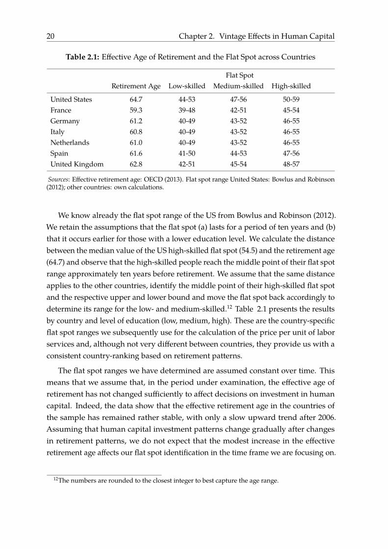
Table 2.1: Effective Age of Retirement and the Flat Spot across Countries
Flat SpotRetirement Age Low-skilled Medium-skilled High-skilled
United States 64.7 44-53 47-56 50-59France 59.3 39-48 42-51 45-54Germany 61.2 40-49 43-52 46-55Italy 60.8 40-49 43-52 46-55Netherlands 61.0 40-49 43-52 46-55Spain 61.6 41-50 44-53 47-56United Kingdom 62.8 42-51 45-54 48-57
Sources: Effective retirement age: OECD (2013). Flat spot range United States: Bowlus and Robinson(2012); other countries: own calculations.
We know already the flat spot range of the US from Bowlus and Robinson (2012).We retain the assumptions that the flat spot (a) lasts for a period of ten years and (b)that it occurs earlier for those with a lower education level. We calculate the distancebetween the median value of the US high-skilled flat spot (54.5) and the retirement age(64.7) and observe that the high-skilled people reach the middle point of their flat spotrange approximately ten years before retirement. We assume that the same distanceapplies to the other countries, identify the middle point of their high-skilled flat spotand the respective upper and lower bound and move the flat spot back accordingly todetermine its range for the low- and medium-skilled.12 Table 2.1 presents the resultsby country and level of education (low, medium, high). These are the country-specificflat spot ranges we subsequently use for the calculation of the price per unit of laborservices and, although not very different between countries, they provide us with aconsistent country-ranking based on retirement patterns.
The flat spot ranges we have determined are assumed constant over time. Thismeans that we assume that, in the period under examination, the effective age ofretirement has not changed sufficiently to affect decisions on investment in humancapital. Indeed, the data show that the effective retirement age in the countries ofthe sample has remained rather stable, with only a slow upward trend after 2006.Assuming that human capital investment patterns change gradually after changesin retirement patterns, we do not expect that the modest increase in the effectiveretirement age affects our flat spot identification in the time frame we are focusing on.
12The numbers are rounded to the closest integer to best capture the age range.
Chapter 2. Vintage Effects in Human Capital 21
2.3 Data
The data we use in order to calculate the price per unit of labor services are from theLuxembourg Income Study Database (LIS, 2017) for the six European countries in ouranalysis – France, Germany, Italy, the Netherlands, Spain, and the United Kingdom.Data for the United States are drawn from the US Current Population Survey, asmade available through IPUMS-CPS.13 LIS collects and harmonizes survey data onsocio-demographic and labor market characteristics, as well as income, at both theindividual- and household-level.14 Data are available for forty-nine countries overmultiple years between 1967 and 2014.
We focus on six European countries over the 1990-2013 period, prioritizing thelarger European countries.15 In processing these data, we have taken special care toensure consistency over time in variable definitions, to ensure comparability acrosscountries and over time. Table 2.2 below lists the main LIS variables we employalongside a short definition.
The sample we analyze in order to construct the prices per unit of labor servicesconsists of men of an age that falls within the country-specific flat spot range we haveidentified. Following Bowlus and Robinson (2012), females are excluded because ofthe fluctuations in their labor force participation. The self-employed are excluded aswell. Furthermore, we only keep those employed full-time, full-year with a positiveincome (larger than one). As full-time full-year, we define those with at least thirty-fiveweekly hours and forty annual weeks worked. Income variables are deflated usingthe consumer price index and (for euro area countries) converted to euros for thefull period. The hourly wage is constructed using information on the annual paidemployment income (pmile) and a person’s weekly hours (hours) and annual weeks(weeks) worked.16
Based on a person’s completed level of education (educ), we derive prices for threecategories of workers, as defined in Table 2.2. We calculate the median hourly wageby age and education level, and subsequently its log change between two points intime. Based on the methodology outlined above (equation 2.3), we then infer changesin the price per unit of labor services. A limitation of the LIS data is that it does not
13See Flood, King, Ruggles, and Warren (2015); this allows us to have an annual time series coveringthe period since 1975.
14LIS uses as data sources national surveys such as the German Socio-Economic Panel (GSOEP) andthe UK’s Family Resources Survey (FRS).
15Expanding the set of countries would lead to shorter time coverage, since complete information onthe required variables is typically a problem, especially when moving back in time.
16For the United Kingdom, data on the number of weeks worked is missing, so ‘full-year’ employmentcannot be used as a criterion and we can only divide the overall employment income by weekly hours.

22 Chapter 2. Vintage Effects in Human Capital
Table 2.2: List of LIS Variables and Definitions
LIS Variable LIS Variable Definition
age Age in years
sex Sex
educ
Highest completed education levelThis variable is recoded into three categories:(a) low: less than secondary education completed (never attended, nocompleted education or education completed at the ISCED levels 0, 1 or 2)(b) medium: secondary education completed (completed ISCED levels3 or 4)(c) high: tertiary education completed (completed ISCED levels 5 or 6)
pmilePaid employment incomeMonetary payments received from regular and irregular dependentemployment
hoursWeekly hours worked, any informationRegular hours worked at all jobs currently held (including family workand overtime, whether paid or unpaid)
weeks Annual weeks worked, any informationNumber of weeks worked during the year in any job
emp EmployedDummy that distinguishes the employed from the non-employed
status1Status in employment (in first job)Variable that distinguishes the dependent-employed from theself-employed
Sources: Documentation-LIS (available online at: http://www.lisdatacenter.org/wp-content/
uploads/our-lis-documentation-variables-definition.xlsx)

Chapter 2. Vintage Effects in Human Capital 23
provide an annual series of surveys. We can directly implement the procedure fromequation 2.3 for the United States, and thus have nine changes in wages to average overthe flat spot range. For the European countries, there is a survey in (for instance) 1993and 1999 for the Netherlands,17 which means that rather than comparing the wageof a 49-year old to that of a 50-year old in the next year, the comparison is between a49-year old in 1993 and a 55-year old in 1999. Since the data for the United States areavailable annually from the CPS, but also at similar intervals in the LIS data, we use acomparison between calculations based on the two sources to establish that the priceseries based on gaps in survey coverage are comparable to those based on annualsurvey data.
In the UK, data on the variable educ are missing for the year 1994, but not forother years in our analysis. We do have information on an individual’s age whencompleted education for 1994, as well as in other years.18 To incorporate data for 1994in the analysis, we identify the typical education level at a given age of educationcompletion. Based on this, we find that low-skilled workers are those who completetheir education at or before the age of 15, medium-skilled between ages 16 and 20 andhigh-skilled are those who complete their education after age 21.
2.4 Results
2.4.1 The price and quantity of labor services per hour worked –United States
An important outcome of our analysis is estimates of the price per unit of labor servicesfor workers of different educational backgrounds. Bowlus and Robinson (2012, Figure3) find that, in the United States, the price per unit of labor services evolves similarlyfor each skill level, which leads them to conclude that changes in relative wagesbetween skills levels represent (primarily) changes in the relative quantity of laborservices per hour worked, rather than changes in relative prices. In Table 2.3, we showthat our own calculations for the US provide a perspective that is not notably different.The first line shows our estimates for the 1975-2014 period, the full length of our studyperiod for the United States. While the price of high-skilled units of labor serviceshas declined by less than that of medium- and low-skilled labor services, this is nota persistent difference.19 The second line shows estimates based on the annual CPS
17See Table A.1 of the appendix for the list of LIS surveys per country that we use in our analysis.18“When he/she last attended continuous full-time education”, variable edcage in LIS.19Our results also closely match those of Bowlus and Robinson (2012, Figure 3).
24 Chapter 2. Vintage Effects in Human Capital
data for 1991-2013, which corresponds to the period for which LIS data are available.The third line shows results based on LIS data for the 1991-2013 period.
Table 2.3: The Change in the Price per Unit of Labor Services in the United States
Change in the Price per Unit of Labor Services
Source Period Low-skilled Medium-skilled High-skilled
CPS 1975-2014 -0.24 -0.20 -0.18
CPS 1991-2013 -0.01 -0.11 -0.06
LIS 1991-2013 -0.02 -0.18 -0.04
Source: Computations based on LIS data (LIS, 2017) and CPS data from IPUMS-CPS (Flood et al., 2015).Notes: The price per unit of labor services is computed based on equation 2.3 and the flat spot rangesin Table 2.1. Each entry in the table indicates the change in price over the stated period, relative to thechange in the country’s consumer price index.
The LIS data, for both the US and Europe, are not available annually but at intervalsof typically three or four years, so lines two and three are useful to gauge the impactof annual data vs. multi-year gaps in the time series. The main difference is thatthe computation of price changes (equation 2.3) can use fewer wage changes if thereare gaps in the time series. For example, with annual data, the wage of 50-year oldhigh-skilled workers in year 1 can be compared to 51-year old high-skilled workersin year 2, all the way to 58-year olds in year 1 and 59-year olds in year 2. As a result,the price change is based on the average of nine wage changes. In contrast, if wagesare observed in year 1 and next in year 4, the price change is an average of 7 wagechanges, comparing 50 year old to 53 year old high-skilled workers until 56 year old to59 year old workers. There is no reason to suspect that this would impart a systematicbias to the price change estimates, but comparing lines 2 and 3 in Table 2.3 allows usto verify this. For low-skilled and high-skilled workers, the differences are small; formedium-skilled workers the differences are larger. Yet, as we show in Figure A.1 of theappendix by charting the full time series for the three skill levels, this larger differenceis not a sign of a systematic deviation between the two sources but a one-off outlier.This gives us greater comfort in relying on LIS data for the analysis of the Europeancountries, below. At the same time, the results in Table 2.3 (as well as those for theEuropean countries, in Table 2.5 below) suggest that the conclusion of ‘no relativeprice changes’ by Bowlus and Robinson (2012) seems not warranted in general. Sowhile Bowlus and Robinson (2012) explicitly disregard relative price movements whenanalyzing changes in the quantity of labor services per hour worked, we will simply

Chapter 2. Vintage Effects in Human Capital 25
use the observed price changes from Table 2.3 (and Table 2.5) when decomposing theoverall wage into a price and quantity component, as in equation 2.1.
Figure 2.1: Labor Services per Hour Worked in the United States, 1975-2014
High-skilled
Medium-skilled
Low-skilled
.7.8
.91
1.1
1.2
1.3
1975=1
1975 1985 1995 2005 2015
Source: Computations based on CPS data from IPUMS-CPS (Flood et al., 2015). Notes: The solidlines show the annual time series of labor services per hour worked, the dashed line is the LOWESStrend estimate (bandwidth of 0.5). Labor services per hour worked are computed by dividing themedian wage of full-time, full-year male workers between the ages of 26 and 60 of a given educationalattainment by the price per unit of labor services of that educational level (see Table 2.3) and normalizedto one in the initial year, 1975.
Figure 2.1 shows the quantity of labor services per hour worked in the United Statesbetween 1975 and 2014, computed by dividing the median wage of (full-time, full-yearmale) workers between the ages of 26 and 60 of a given educational attainment by theprice per unit of labor services for that level of educational attainment, i.e. by applyingequation 2.1. The figure shows the annual series (solid line) as well as an estimate ofthe longer-run trend, computed using a LOWESS smoother with a bandwidth of 0.5.20
The labor services per hour of high-skilled workers increased substantially over thisperiod, rising by 25 percent compared to 1975, with most of this increase (19 percent)
20The LOWESS smoother creates a curve to best capture the trend of labor services per hour worked.It is the result of a locally weighted regression of labor services per hour worked on time/year.

26 Chapter 2. Vintage Effects in Human Capital
occurring between 1995 and 2005. There has been a decline in labor services per hourworked of medium-skilled workers of approximately 10 percent, with a sustaineddecline between 1975 and 1995 and fluctuations around this level in the subsequentperiod. Labor services per hour worked of low-skilled workers also declined, by20 percent, with sustained declines between 1975 and 1995. This periodization issomewhat arbitrary, also given the, sometimes large, year-to-year fluctuations in theseries. The estimated trends suggest that salience of the 1975-1995 period for medium-and low-skilled workers and of the 1995-2005 period for high-skilled workers may notbe as large, but notable differences remain in the pattern of changes over time.
Table 2.4: Linear Time Trend of Labor Services per Hour Worked in the United States,1975-2014
Low-skilled Medium-skilled High-skilled
Age 26-60 -0.0067*** -0.0007 0.0069***
(0.0004) (0.0004) (0.0003)
Age 26-35 -0.0044*** -0.0015** 0.0052***
(0.0007) (0.0007) (0.0004)
Age 36-45 -0.0058*** -0.0025*** 0.0056***
(0.0005) (0.0003) (0.0005)
Notes: N=40. Each entry in the table is the coefficient of a linear time trend on the log of labor servicesper hour worked in a given age range and level of educational attainment. Robust standard errors aregiven in parentheses; *** p<0.01, ** p<0.05, * p<0.1.
To establish that the patterns in Figure 2.1 are not mere noise in a statistical sense,the first row of Table 2.4 shows the coefficients of a linear time trend for the (log of)labor services per hour worked for the age range 26 to 60. This shows a significantnegative time trend for low-skilled workers, no significant time trend for medium-skilled workers, and a positive time trend for high-skilled workers. The subsequentrows test the sensitivity of this result and show that similar time trends can be observedfor narrower age ranges, though with a significantly negative time trend for medium-skilled workers as well. This indicates that the patterns are observed broadly acrossthe (male) population.
Chapter 2. Vintage Effects in Human Capital 27
2.4.2 The price and quantity of labor services per hour worked –Europe
We next turn to the European countries, analyzing the trends in relative price and thenquantities of labor services. The price developments, shown in Table 2.5, are moremixed than in the US, with, for example, France showing similar price trends acrosseducational categories, Germany showing price declines for low-skilled and priceincreases for high-skilled and the United Kingdom showing the reverse pattern ofprice increases for low-skilled and price decreases for high-skilled labor services. Thisvariety of patterns remains intact through a range of sensitivity checks (see below)and does not lend itself to easy explanation. This more firmly establishes the need toaccount for these price changes when analyzing the trends in the quantity of laborservices per hour worked.
Table 2.5: The Change in the Price per Unit of Labor Services in Europe
Change in the Price per Unit of Labor Services
Country Period Low-skilled Medium-skilled High-skilled
France 1994-2005 0.12 0.17 0.14
Germany 1994-2013 -0.15 0.07 0.36
Italy 1991-2010 0.04 0.01 0.12
Netherlands 1990-2013 0.07 0.06 0.13
Spain 2007-2013 -0.01 0.15 0.10
United Kingdom 1994-2013 0.11 -0.24 -0.27
Source: Computations based on LIS data (LIS, 2017). Note: The price per unit of labor services iscomputed based on equation 2.3 and the flat spot ranges in Table 2.1. Each entry in the table indicatesthe change in price over the stated period, relative to the change in the country’s consumer price index.
To analyze the trends in the quantity of labor services per hour worked acrossEuropean countries, we first pool the country-level results. We compute a weightedaverage across the six European countries of labor services per hour worked, firstlinearly interpolating between LIS-covered years and then using the share of eachcountry in total employment by educational attainment as weights.21 Due to variation
21Using data from the WIOD Socio-Economic Accounts (Timmer, Dietzenbacher, Los, Stehrer, & deVries, 2015). We assume that workers in the UK work 40 weeks per year to accommodate missing dataon this variable in LIS.

28 Chapter 2. Vintage Effects in Human Capital
in country coverage over time, we construct a ‘Europe’ series starting in 1994 andending in 2013.
Figure 2.2 shows the development of the quantity of labor services per hour workedfor the six European countries, on the same scale as Figure 2.1 for the United States.There is no clear trend over time in the quantity of labor services per hour worked forany level of educational attainment. This is especially true when taking the year-to-year swings into account, i.e. it is hard to discern a trend if an increase or decrease of6 percent in labor services per hour worked can be observed.22
Figure 2.2: Labor Services per Hour Worked in Europe, 1994-2013
High-skilled
Medium-skilled
Low-skilled
.7.8
.91
1.1
1.2
1.3
1994=1
1995 2000 2005 2010 2015
Source: Computations based on LIS data (LIS, 2017). Notes: The solid lines show the annual time seriesof labor services per hour worked, the dashed line is the LOWESS trend estimate (bandwidth of 0.5).Labor services per hour worked are computed by dividing the median wage of full-time, full-year maleworkers between the ages of 26 and 60 of a given educational attainment by the price per unit of laborservices of that educational level (see Table 2.5) and normalized to one in the initial year, 1994. Thefigure shows a weighted average of labor services per hour worked across the six European countriescovered (see Table 2.5), using total employment by educational attainment of a country as weights.
This is further confirmed in Table 2.6, which shows the results from regressions of22Although there seem to be increases in recent years (after the Great Recession), these may be (at
best) the start of a longer trend rather than an established pattern. Moreover, there is no difference byskill level, so even if this were a clear trend, it would be one of a different pattern.
Chapter 2. Vintage Effects in Human Capital 29
a linear time trend on the log of labor services per hour worked for all observations forthe six European countries. The regressions include country fixed effects as the periodcovered in each country differs (though results are not substantively different withoutfixed effects). The only common finding across age groups is that labor servicesper hour worked of low-skilled workers have declined, though the rate of decline issmaller than observed in the US (cf. Table 2.4).
Table 2.6: Linear Time Trend of Labor Services per Hour Worked in Europe,1990-2013
Low-skilled Medium-skilled High-skilled
Age 26-60 -0.0026* 0.0000 -0.0033
(0.0012) (0.0027) (0.0037)
Age 26-35 -0.0062** -0.0035 -0.0084*
(0.0022) (0.0036) (0.0039)
Age 36-45 -0.0041** -0.0019 -0.0036
(0.0011) (0.0022) (0.0040)
Notes: N=33. Each entry in the table is the coefficient of a linear time trend on the log of labor servicesper hour worked in a given age range and level of educational attainment. All 33 observations as wellas country fixed effects for the six European countries are included in each regression. Robust standarderrors are given in parentheses; *** p<0.01, ** p<0.05, * p<0.1.
Despite these inconclusive patterns for the period as a whole and the full set ofEuropean countries, a clearer distinction becomes apparent when zooming in on theperiod of 1995 to 2005. For the United States, this was the period in which the largestincreases in labor services per hour worked by high-skilled workers could be seen,in Figure 2.1, and this is shown in the first line of Table 2.7. When selecting the LISsurvey years of each European country to most closely match the 1995-2005 period,23
the United Kingdom stands out amongst the European countries in showing a 25percent increase in labor services per hour worked by high-skilled workers, while thefour Continental European countries show declines of 10 to 14 percent. For low-skilledand medium-skilled workers the changes in the quantity of labor services per hourworked are typically smaller than for high-skilled workers, though the UK also shows
23Spain is not shown in the table because its price series is only available from 2007 onwards, seeTable A.1 of the appendix.
30 Chapter 2. Vintage Effects in Human Capital
Table 2.7: The Change in the Quantity of Labor Services per Hour Worked in Europeand the United States between the mid-1990s and mid-2000s
Change in the Quantity of Labor Servicesper Hour Worked
Low-skilled Medium-skilled High-skilled
United States 1995-2005 0.01 0.01 0.19United Kingdom 1994-2004 -0.09 0.22 0.25
France 1994-2005 -0.04 -0.10 -0.14Germany 1994-2004 0.01 -0.04 -0.10Italy 1995-2004 0.00 0.00 -0.09Netherlands 1993-2004 0.02 0.02 -0.10
Notes: See Notes to Figures 2.1 and 2.2. Spain is not shown because its data series starts in 2007.
a notable increase for medium-skilled workers. Before turning to the implications ofthe differences for high-skilled workers for measured productivity, we first assess thesensitivity of the results to the assumptions and choices we made.
2.4.3 Sensitivity analysis
Computing the prices per unit of labor services involves a series of choices and judge-ments, as the preceding discussion has already illustrated. Of particular note is thedetermination of the flat spot range. Bowlus and Robinson (2012) devote considerableattention to this topic, for instance by showing that moving the flat spot range for high-skilled workers to earlier ages would pick up some of the upward-sloping wages in astandard, concave earnings-experience profile. We have anchored our own analysisto that of Bowlus and Robinson (2012) by using their US flat spot range and adjustingit to reflect differences in effective retirement age. An alternative is to directly use theUS flat spot range for European countries.
In addition, we consider a range of treatments of the European LIS data. Whatour results for the United States (Table 2.3) already indicated is that the frequency ofsurvey data availability is not an important source of sensitivity, nor is the numberof educational categories considered (four in Bowlus and Robinson (2012), threein this study). A potential concern could be that the price series we estimate are‘contaminated’ with noise. A reason could be a small number of full-time full-yearmale survey respondents in an education/age cell, which could give wage outliersan undue influence on the final price series. By taking the median wage of each
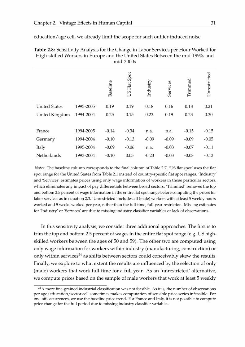
Chapter 2. Vintage Effects in Human Capital 31
education/age cell, we already limit the scope for such outlier-induced noise.
Table 2.8: Sensitivity Analysis for the Change in Labor Services per Hour Worked forHigh-skilled Workers in Europe and the United States Between the mid-1990s and
mid-2000s
Base
line
US
Flat
Spot
Indu
stry
Serv
ices
Trim
med
Unr
estr
icte
d
United States 1995-2005 0.19 0.19 0.18 0.16 0.18 0.21
United Kingdom 1994-2004 0.25 0.15 0.23 0.19 0.23 0.30
France 1994-2005 -0.14 -0.34 n.a. n.a. -0.15 -0.15
Germany 1994-2004 -0.10 -0.13 -0.09 -0.09 -0.09 -0.05
Italy 1995-2004 -0.09 -0.06 n.a. -0.03 -0.07 -0.11
Netherlands 1993-2004 -0.10 0.03 -0.23 -0.03 -0.08 -0.13
Notes: The baseline column corresponds to the final column of Table 2.7. ‘US flat spot’ uses the flatspot range for the United States from Table 2.1 instead of country-specific flat spot ranges. ‘Industry’and ‘Services’ estimates prices using only wage information of workers in those particular sectors,which eliminates any impact of pay differentials between broad sectors. ‘Trimmed’ removes the topand bottom 2.5 percent of wage information in the entire flat spot range before computing the prices forlabor services as in equation 2.3. ‘Unrestricted’ includes all (male) workers with at least 5 weekly hoursworked and 5 weeks worked per year, rather than the full-time, full-year restriction. Missing estimatesfor ‘Industry’ or ‘Services’ are due to missing industry classifier variables or lack of observations.
In this sensitivity analysis, we consider three additional approaches. The first is totrim the top and bottom 2.5 percent of wages in the entire flat spot range (e.g. US high-skilled workers between the ages of 50 and 59). The other two are computed usingonly wage information for workers within industry (manufacturing, construction) oronly within services24 as shifts between sectors could conceivably skew the results.Finally, we explore to what extent the results are influenced by the selection of only(male) workers that work full-time for a full year. As an ‘unrestricted’ alternative,we compute prices based on the sample of male workers that work at least 5 weekly
24A more fine-grained industrial classification was not feasible. As it is, the number of observationsper age/education/sector cell sometimes makes computation of sensible price series infeasible. Forone-off occurrences, we use the baseline price trend. For France and Italy, it is not possible to computeprice change for the full period due to missing industry classifier variables.
32 Chapter 2. Vintage Effects in Human Capital
hours and 5 weeks per year. In Table 2.8, we show how the baseline results in the finalcolumn of Table 2.7 change for these alternatives.25
As the table shows, the different price series influence the change in the quantityof labor services per hour worked relative to the baseline estimate. Yet the overallpattern remains similar: the United States and United Kingdom show increasing laborservices per hour worked for high-skilled workers, while the Continental Europeancountries show predominantly declines. Relying on the US flat spot range ratherthan our country-specific ranges has a varied impact on the Continental Europeancountries, with larger declines in France but even a small increase in the Netherlands.Selecting workers only in Industry or in Services leads to somewhat smaller changes inthe quantity of labor services per hour worked in some of the countries, but again, nosubstantive changes. Outliers in wage data do not seem to have a systematic impact asthe change in the quantity of labor services per hour worked for the Trimmed series isbarely different from the baseline. Finally, using a less restrictive sampling of workersto compute the change in price of labor services per hour worked leads to somewhatlarger changes, but again, no substantial deviation from the baseline results.
2.4.4 Implications for Europe-US productivity growth comparisons
Our main finding is that labor services per hour worked of high-skilled workers inthe United States and United Kingdom increased by 19-25 percent between 1995 and2005, while Continental European countries register declines of 10-14 percent overthe similar period. This is a finding that can have important implications for produc-tivity growth comparisons between Europe and the United States. Standard growthaccounting assumes constant labor services per hour worked over time in estimating(multifactor) productivity growth, but if this assumption is violated, productivitygrowth will have been overestimated in the United States and United Kingdom andunderestimated in Continental European countries. Between 1995 and 2005, produc-tivity growth in the United States was much higher than before or since (Byrne et al.,2016; Syverson, 2017) and much higher than in Europe (e.g. van Ark et al., 2008). Ifwe zoom in on the market economy – which excludes government, health, educationand real estate – US productivity growth was 1.4 percent on average per year between1995 and 2005, while growth averaged a mere 0.6 percent between 1975 and 1995
25The estimates for low and medium-skilled workers do not show a clear pattern and are thereforeomitted. These data are available on request.

Chapter 2. Vintage Effects in Human Capital 33
and 0.1 percent between 2005 and 2014.26 In contrast, European countries showednotably lower productivity growth over this period, see also Table 2.9, below. A largeliterature has aimed to explain this growth gap focusing on explanations such aslower investment in R&D and stricter regulations or the role of ICT-producing andICT-using industries; see e.g. the survey of Ortega-Argiles (2012). Yet our analysispoints to a hitherto underappreciated element. While differences in human capitalaccumulation have typically been found wanting as an explanatory factor, relaxingthe ‘constant labor services per hour worked’ assumption may provide greater heft tothis factor.
To gauge the importance of our findings for the Europe-US productivity growthdifference, consider the following expression for (Solow residual) productivity growth:
∆logA = ∆logV − α∆logK − (1 − α)∆logL (2.4)
where ∆ is the difference operator, A is productivity, V is value added,K is capitalinput, L is labor input, and α is the output elasticity of capital – typically assumed tobe equal to the share of capital income in value added. This implies assuming perfectcompetition in factor and output markets and a constant returns to scale productionfunction. Labor input is typically distinguished by type of worker, assuming that agiven type of worker (denoted by j) provides a constant quantity of labor services perhour worked over time. If that type of worker’s marginal product equals its marginalcost, the share of total labor compensation flowing to that type of worker (wj) can beused to weight the growth in hours worked by that type of worker,Hj :
∆logL =N∑j=1
wj∆logHj (2.5)
But if, as we have established, the effective labor input per hour worked of aparticular type of worker changes over time, we should adjust our computation of thegrowth in overall labor services:
∆logL∗ =N∑j=1
wj∆log(Hj · Ej) (2.6)
Here Ej is an estimate of effective labor services per hour worked. Note that thelabor compensation share wj of each labor type is the same in both equations, as total
26The 1975-2005 data are drawn from the 2012 version of the EU KLEMS database; see O’Mahonyand Timmer (2009). The 2005-2014 average is computed using BLS data for the private business sector,which showed similar growth as the EU KLEMS market economy between 1995 and 2005.

34 Chapter 2. Vintage Effects in Human Capital
labor compensation does not depend on the division of that sum between a price anda quantity component. Denote as ∆logA∗ the estimate of productivity growth basedon adjusted growth in labor services, so substituting ∆logL by ∆logL∗ in equation 2.4:
∆logA∗ = ∆logV − α∆logK − (1 − α)∆logL∗ (2.4’)
To implement equations 2.5 and 2.6, we use data on hours worked (Hj) and theshare of labor compensation (wj) of low-, medium-, and high-skilled workers for theUnited States and the six European countries.27 All Ej are set equal to one, exceptfor those of high-skilled workers between 1995 and 2005. For those years and thattype, we set the annual Ej such that the quantity of labor services per hour worked byhigh-skilled workers increases by the amount shown in the final column of Table 2.7.This assumes that our estimates of the increase in labor services per hour workedof (full-time, full-year) male workers is applicable for all workers. As discussed inBowlus and Robinson (2012), this may be an overestimation, because of changes inthe degree of discrimination of women in the labor market. Such changes, though,may be relatively modest over a ten year period.
Table 2.9 presents standard growth accounting results based on EU KLEMS aswell as figures adjusted for the vintage effects for high-skilled workers that we foundin Table 2.7 for the period 1995 to 2005. The average annual growth of high-skilledlabor input is shown first, with changes in total hour worked shown under ‘StandardGrowth Accounting’ and changes in total labor services under ‘Adjusted for VintageEffects’. So, for example, total hours worked of high-skilled workers grew at anaverage annual rate of 1.9 percent in the US over this period. The final column inTable 2.7 showed that labor services per hour worked of US high-skilled workersincreased by 19 percent over this 10-year period, which corresponds to an averageannual increase of 1.8 percent. Therefore, labor services of high-skilled increased atan average annual rate of 3.7 percent, as shown under ‘Adjusted for Vintage Effects’.We can then apply equations 2.5 and 2.6 to show that total labor services grew 0.7(1.7-1.0) percentage points faster when adjusting for vintage effects than based onstandard growth accounting assumptions.28 This translates to an average annual TFP
27These data are not available in the 2012 version of EU KLEMS, but are presented in WIOD’s Socio-Economic Accounts (Timmer et al., 2015), so we use those data and combine them with TFP growthestimates from EU KLEMS. Also note that these shares are not constant over time, so we computetwo-period average compensation shares to implement equations 2.5 and 2.6 as a Tornqvist index.Similarly, we use the two-period average share of capital income in value added in implementingequations 2.4 and 2.4’.
28Labor compensation of high-skilled workers accounted for, on average, 31 percent of total laborcompensation in the US over this period.
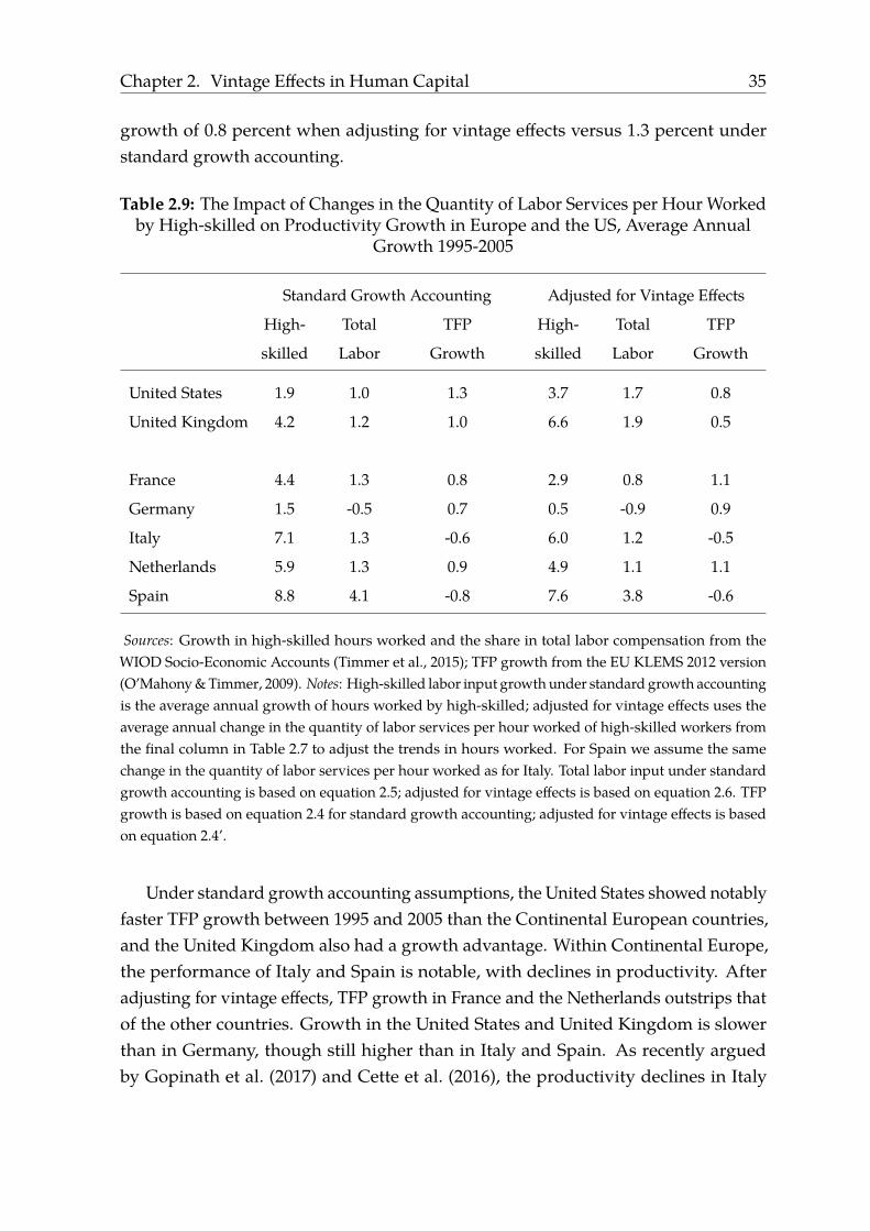
Chapter 2. Vintage Effects in Human Capital 35
growth of 0.8 percent when adjusting for vintage effects versus 1.3 percent understandard growth accounting.
Table 2.9: The Impact of Changes in the Quantity of Labor Services per Hour Workedby High-skilled on Productivity Growth in Europe and the US, Average Annual
Growth 1995-2005
Standard Growth Accounting Adjusted for Vintage Effects
High- Total TFP High- Total TFP
skilled Labor Growth skilled Labor Growth
United States 1.9 1.0 1.3 3.7 1.7 0.8
United Kingdom 4.2 1.2 1.0 6.6 1.9 0.5
France 4.4 1.3 0.8 2.9 0.8 1.1
Germany 1.5 -0.5 0.7 0.5 -0.9 0.9
Italy 7.1 1.3 -0.6 6.0 1.2 -0.5
Netherlands 5.9 1.3 0.9 4.9 1.1 1.1
Spain 8.8 4.1 -0.8 7.6 3.8 -0.6
Sources: Growth in high-skilled hours worked and the share in total labor compensation from theWIOD Socio-Economic Accounts (Timmer et al., 2015); TFP growth from the EU KLEMS 2012 version(O’Mahony & Timmer, 2009). Notes: High-skilled labor input growth under standard growth accountingis the average annual growth of hours worked by high-skilled; adjusted for vintage effects uses theaverage annual change in the quantity of labor services per hour worked of high-skilled workers fromthe final column in Table 2.7 to adjust the trends in hours worked. For Spain we assume the samechange in the quantity of labor services per hour worked as for Italy. Total labor input under standardgrowth accounting is based on equation 2.5; adjusted for vintage effects is based on equation 2.6. TFPgrowth is based on equation 2.4 for standard growth accounting; adjusted for vintage effects is basedon equation 2.4’.
Under standard growth accounting assumptions, the United States showed notablyfaster TFP growth between 1995 and 2005 than the Continental European countries,and the United Kingdom also had a growth advantage. Within Continental Europe,the performance of Italy and Spain is notable, with declines in productivity. Afteradjusting for vintage effects, TFP growth in France and the Netherlands outstrips thatof the other countries. Growth in the United States and United Kingdom is slowerthan in Germany, though still higher than in Italy and Spain. As recently arguedby Gopinath et al. (2017) and Cette et al. (2016), the productivity declines in Italy

36 Chapter 2. Vintage Effects in Human Capital
and Spain can be traced to a deterioration of the capital allocation process. Thatdeterioration, in turn, was triggered by the decline in real interest rates in the run-upto Italy and Spain joining the euro. In other words, the productivity declines in thesecountries were due to exceptional circumstances, while the other five countries inthe table had broadly comparable productivity growth rates between 1995 and 2005.This implies that the most notable difference between Anglo-Saxon and ContinentalEuropean countries is in their human capital vintage effects.
2.5 Conclusions
This paper has contributed to a growing literature that emphasizes human capitalaccumulation after formal education as an important factor for understanding therole of human capital in the process of economic growth and for understanding cross-country income differences. In growth accounting (or development accounting) astandard assumption is that an hour worked by a worker of given type, e.g. high-skilled males, represents a constant amount of labor services per hour worked overtime. Yet if there are vintage effects, this assumption may be violated. Our startingpoint is recent research that identified vintage (or cohort) effects for the United States(Bowlus & Robinson, 2012) and we extended their methodology to six Europeancountries. The starting point in their methodology is that the ‘constant labor servicesper hour worked’ assumption only holds for workers in the later stage of their workinglife, when the incentive to invest in human capital has disappeared – the so-calledflat spot range. Vintage effects can then be identified from wage changes for youngerworkers relative to wage changes of workers in the flat spot range.
We confirm the findings for the United States of Bowlus and Robinson (2012) ofvintage effects, with declining labor services per hour worked for low- and medium-skilled workers between 1975 and 1995 and rapidly increasing labor services per hourworked by high-skilled workers between 1995 and 2005. We find similar vintageeffects in the United Kingdom, with even larger increases in labor services per hourworked by high-skilled workers over the same period. In contrast, we find evidence ofdeclining labor services per hour worked by high-skilled workers in the ContinentalEuropean countries, in a notable divergence.
This divergence in vintage effects has a notable impact on the productivity growthdifference between the US and UK, on the one hand, and the Continental Europeancountries – France, Germany, Italy, Netherlands and Spain – on the other hand. Theincreases of labor services per hour worked in the US and UK imply faster growth of

Chapter 2. Vintage Effects in Human Capital 37
labor input and, hence, smaller productivity growth. The opposite is the case for theContinental European countries. The net result of these adjustments is that the USand UK no longer show faster productivity growth than the Continental Europeancountries.
On one level, this is an encouraging result, because it provides a novel perspectiveon the Europe-US productivity growth difference and because the set of reasons forwhy productivity growth is high or low can be considerably larger than the set ofreasons for why vintage effects were so different in the US and UK compared to theContinental European countries. At the same time, the Bowlus and Robinson (2012)methodology only pinpoints vintage effects but it does not provide an explanationfor why they occur. It is also an open question to what extent the evidence for maleworkers can be generalized to female workers. We leave these important issues forfuture research.


APPENDIX A
Appendix Chapter 2
Figure A.1: Price Series for the United States Based on CPS and LIS Data for 1991-2013
.8.85
.9.95
11.05
Price(1991=1)
1990 1995 2000 2005 2010 2015
CPS LIS
Low-skilled.8
.85
.9.95
11.05
Price(1991=1)
1990 1995 2000 2005 2010 2015
CPS LIS
Medium-skilled
.8.85
.9.95
11.05
Price(1991=1)
1990 1995 2000 2005 2010 2015
CPS LIS
High-skilled
39
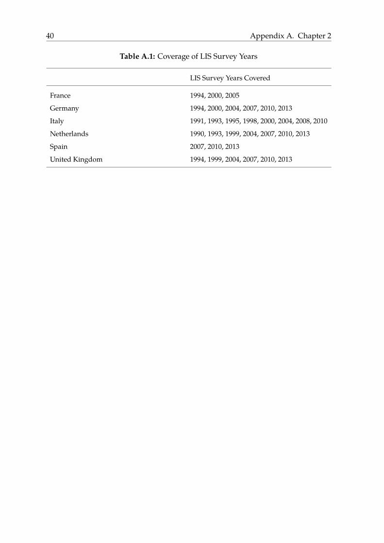
40 Appendix A. Chapter 2
Table A.1: Coverage of LIS Survey Years
LIS Survey Years Covered
France 1994, 2000, 2005
Germany 1994, 2000, 2004, 2007, 2010, 2013
Italy 1991, 1993, 1995, 1998, 2000, 2004, 2008, 2010
Netherlands 1990, 1993, 1999, 2004, 2007, 2010, 2013
Spain 2007, 2010, 2013
United Kingdom 1994, 1999, 2004, 2007, 2010, 2013
CHAPTER 3
Composition of Human Capital, Distance to the Frontierand Productivity∗
3.1 Introduction
Human capital, commonly captured in empirical research by a country’s level ofeducation, has been identified as a key determinant of economic growth: it trig-
gers innovation (Romer, 1990), facilitates the adoption of new technologies developedby the world’s technological leader (Nelson & Phelps, 1966) and affects output directlybeing itself a factor of production (Mankiw et al., 1992).1 Yet, in a seminal contribution,Krueger and Lindahl (2001, p. 1130) find only ‘fragile’ empirical evidence in favorof externalities stemming from human capital. The latter would emerge in the formof technological progress, presumably through facilitating innovation and imitation,that is, the adoption of already existing technologies.2
This hypothesis has received much attention in the literature. In a widely citedpaper, Vandenbussche et al. (2006) show that a greater share of university-educatedworkers stimulates innovation but only for countries that are relatively close to thetechnology frontier. Ang et al. (2011) confirm this finding for both high- and medium-income countries, and also show that low-income ones do not benefit from externalities.Cerina and Manca (2016), on the contrary, argue that countries far from the technology
∗For an earlier version of this chapter, see Papakonstantinou (2014). I would like to thank WenChen, Robert Inklaar, Bart Los, Petros Milionis, Pierre Pecher, Laurie Reijnders, Marcel Timmer andparticipants at the SOM PhD Conference (University of Groningen, The Netherlands, March 2014), the33rd IARIW General Conference (Rotterdam, The Netherlands, August 2014), the 20th Spring Meetingof Young Economists (Ghent, Belgium, May 2015) and the 14th European Workshop on Efficiency andProductivity Analysis (Helsinki, Finland, June 2015) for helpful comments and suggestions.
1For reviews on the role of human capital for economic growth, see: Krueger and Lindahl (2001);Sianesi and van Reenen (2003); Savvides and Stengos (2009); Benos and Zotou (2014); Delgado et al.(2014); Glewwe et al. (2014).
2Although outside the scope of this paper, the literature has also identified other types of externalities(see, for example, Lochner (2011) on the non-production benefits of education).
41

42 Chapter 3. Composition of Human Capital
frontier do benefit from a high-skilled workforce by means of technology adoption.At the industry-level, Inklaar et al. (2008) and Mason, O’Leary, and Vecchi (2012) findno compelling externalities evidence.
The externalities literature has devoted considerable attention to the constructionof appropriate data on the educational attainment level of the workforce and howthe quality of these data affects the education-growth relationship.3 But much lessattention has been devoted to the construction of appropriate productivity measures,even though the results could be sensitive to this as well. In order to study externalities,we need to distinguish between private and social returns to education in a growthaccounting measure of productivity. The private returns should be captured by ameasure of labor input that weights hours worked by their wage, also known ascorrecting for labor force quality. Any additional benefit from education not reflectedin a higher (relative) wage, will end up in TFP which is residually measured. Thus,to properly measure externalities we require a TFP measure that accounts for inter-country differences in the educational composition of the workforce otherwise TFPwill be mismeasured (Inklaar et al., 2008; Mason et al., 2012). However, Vandenbusscheet al. (2006), Ang et al. (2011) and Cerina and Manca (2016) use a crude TFP measurethat does not control for the above. According to Inklaar et al. (2008), any evidence ofexternalities of human capital disappears when an education-adjusted productivitymeasure is employed. Mason et al. (2012) reach a similar result.
The contribution of this paper is, thus, to use the state-of-the-art cross-countryproductivity measures available in the recent version of the Penn World Table (PWT)4
to determine how widely the evidence extends in favor of externalities stemming fromhuman capital. I focus on three types of human capital that refer to a country’s shareof the population with tertiary, secondary and primary educational attainment (ora country’s average years of tertiary, secondary and primary schooling attained).5 Istudy their impact on TFP growth by means of a panel (country-time) fixed effectsregression analysis. My sample includes 106 developed and developing countriesbetween 1970-2010. Furthermore, I allow the effect of tertiary and secondary educationon TFP growth to vary with a country’s distance from the world technology frontier.6
My analysis points to broader and more robust evidence of externalities than the3See, for example, Portela, Alessie, and Teulings (2010).4Specifically version 8.0 of the PWT (Feenstra, Inklaar, & Timmer, 2015) that calculates education-
adjusted TFP measures. The section on TFP data below presents additional information on the con-struction of such residual TFP measures.
5Education data come from the latest version (2.0) of the Barro and Lee (2013) dataset on educationalattainment.
6Following similar studies in the literature (e.g. Vandenbussche et al., 2006), the United Statesconstitute the world’s technology frontier.

Chapter 3. Composition of Human Capital 43
literature so far as I find strong evidence of positive externalities from tertiary-educatedworkers. The results suggest positive externalities for all countries, even those far fromthe technology frontier. In line with Vandenbussche et al. (2006) and Ang et al. (2011),I find that university-educated workers contribute to faster productivity growth forcountries close to the frontier compared to countries some distance away. At evengreater distance, though, a large positive effect is found again, in line with Cerinaand Manca (2016). Stated differently, the marginal effect of tertiary education on TFPgrowth is U-shaped: it is large for countries far from the world technology frontier,decreases as countries move closer to it and, from a point onwards, increases again.This increase, however, is relatively small in magnitude. I also find some evidenceof externalities from secondary education. These are limited though to a number ofmiddle- and/or low-income countries.
Vandenbussche et al. (2006) suggest one major shift in the growth process, fromgrowth primarily based on imitation, facilitated by non-high-skilled workers, toinnovation, which is facilitated by high-skilled, university-educated workers. Theresults of Ang et al. (2011) serve mostly to strengthen the evidence for this particularshift. My results point to another shift, related to Cerina and Manca (2016), whereuniversity-educated workers also significantly contribute to imitation-led growth.This finding is consistent with technology diffusion models whereby human capitalenhances a country’s ability for technology adoption (e.g. Nelson & Phelps, 1966;Benhabib & Spiegel, 1994, 2005).7 Finally, I find that using a crude, rather than aneducation-adjusted, TFP measure does not alter the core conclusions of my analysis.The latter is still preferred though as the, conceptually, most appropriate measurewhen studying externalities.
My main result of broad externalities from tertiary-educated workers is robust todifferent measures of education (such as the average years of tertiary schooling ratherthan the share of university-educated workers) and age groups (people aged 15 or25 and above and people aged 25-64), as well as to alternative estimation strategies(OLS and instrumental variables estimation). Throughout the paper, I also considerdifferent functional forms (with or without interaction terms) and groups of countries(full sample with developed and developing economies versus restricted sample withonly advanced OECD countries).
The paper proceeds as follows: The subsequent section introduces the empiricalmodel, Section 3.3 presents the data and Section 3.4 the results. Section 3.5 concludes.
7Other studies that distinguish between types of human capital and also introduce the concepts ofinnovation and imitation are: Benhabib and Spiegel (1994, 2005); Benhabib, Perla, and Tonetti (2014);Madsen (2014); Squicciarini and Voigtlander (2015).
44 Chapter 3. Composition of Human Capital
3.2 The Model
My baseline model to estimate the effect of human capital on TFP growth draws onthe work of Vandenbussche et al. (2006). It is of a panel (country-time) form andcovers 106 countries in five-year intervals over the period 1970-2010. More specifically,I will estimate the following equation:
gi,t = λi + µt + α · ln(Pi,t−5) + β′ ·HCi,t−5 + γ′ ·Xi,t + εi,t (3.1)
where the dependent variable gi,t = ∆ln(rtfpnai,t) = ln(rtfpnai,t)−ln(rtfpnai,t−5)
denotes productivity growth of country i between time t−5 and t. The variable rtfpnastands for TFP at constant national prices and is derived from PWT 8.0 (Feenstra et al.,2015). Note that I study productivity growth in five-year intervals. This is not only dueto (human capital) data availability8, but also because research has suggested that cross-country growth estimations are more robust when five-year intervals are employed,at least compared to annual ones (Johnson, Larson, Papageorgiou, & Subramanian,2013). The main regressors of the analysis are: (i) the logarithm of the proximity (ordistance) to the TFP frontier, ln(Pi,t−5) and (ii) the human capital of country i, HCi,t−5,both of which refer to the beginning of the period.
To calculate P , the United States act as the frontier, as commonly done in the litera-ture (see, for example, Vandenbussche et al. (2006); Ang et al. (2011)). More specifically,the proximity variable is calculated as: ln(Pi,t−5) = ln(ctfpi,t−5/ctfpUSA,t−5), wherectfp denotes the TFP level at current PPPs and comes from PWT 8.0 (Feenstra etal., 2015).9 Note, at this point, that I use two different TFP variables from PWT formy analysis, rtfpna (for the dependent) and ctfp (for the independent variable), thereason being that the former is most suited for comparisons within a country overtime, whereas the latter mainly facilitates comparisons between countries at one pointin time.10 Note, also, that ln(Pi,t−5) is a negative number since I only focus on countriesthat have lower TFP levels than the US (I require ln(Pi,t−5) ≤ 0). Hence, the larger thevalue of ln(Pi,t−5), the closer a country is to the frontier (stated differently, there is arelatively smaller technological distance between that country and the US). There are,however, countries in the PWT dataset which, for some years, have scored higher inTFP than the US. I have removed these observations from the analysis, since a storyabout the drivers of productivity growth makes more intuitive sense when it refers to
8The Barro and Lee (2013) dataset that I use for my education variables provides information for146 countries between 1950-2010, in five-year intervals.
9The variable ctfp is already computed relative to the US in PWT 8.0.10For details, see Feenstra et al. (2015), Inklaar and Timmer (2013) and the discussion in Section 3.3.

Chapter 3. Composition of Human Capital 45
countries that lie below the frontier and try to catch up. I have opted for the US asthe world technology frontier, first, because other countries do not consistently (for allyears) score higher in productivity and, also, because the US has commonly acted asthe frontier in the literature. Furthermore, relatively small economies (e.g. Sweden,Norway) or countries with a large petroleum industry (e.g. Kuwait, Saudi Arabia)may have high(er) TFP levels but cannot adequately represent the world technologyfrontier for all sectors of an economy (Madsen, 2014).
Human capital (HCi,t−5 in model 3.1) enters my empirical analysis through threealternative measures: (i) tertiary (T HCi,t−5), (ii) secondary (S HCi,t−5), and (iii) pri-mary (P HCi,t−5) education. Depending on the specification, these three measures(types of human capital) are either captured by a country’s average years of tertiary,secondary and primary schooling or the percentage of the population with tertiary,secondary and primary education. Unless otherwise specified, the variables refer tothe population aged 25 and above and come from the latest version (2.0) of the Barroand Lee (2013) dataset on educational attainment. Important to note is that, at a laterstage, I augment baseline model 3.1 with interaction terms between human capitaland proximity to the frontier (e.g. ln(Pi,t−5) · T HCi,t−5; ln(Pi,t−5) · S HCi,t−5). I doso in order to examine the role of education for countries at different distances fromthe world technological leader and, also, to identify the effects of education on TFPgrowth under different functional forms.
Finally, the model incorporates a set of control variables (Xi,t). Following Ang etal. (2011), this includes (i) inflationi,t, measured by the consumer price index anddefined as the annual percentage change in the cost of acquiring a basket of goods andservices; (ii) tradei,t, captured by the sum of exports and imports of goods and servicesas a percentage of GDP; (iii) fdii,t, namely the net inflows of foreign direct investmentas a percentage of GDP; and (iv) crediti,t, defined as the domestic credit to privatesector, again, as a percentage of GDP.11 All control variables come from the WorldDevelopment Indicators (WDI, 2015) and are calculated as averages between timet− 5 and t, following Ang et al. (2011). Table B.2 of the appendix provides summarystatistics for all variables.
The empirical analysis is based on OLS (country) fixed effects regressions whichalso incorporate a set of time dummies. Country- (λi) and time-specific (µt) factors that
11Ang et al. (2011) also include a variable to control for a country’s geographical location. As I amperforming fixed effects regressions, the impact of such time-invariant variable is already accountedfor. I also considered the impact of institutions on TFP growth by adding a control variable for thelegal system and security of property rights from the Fraser Institute (Gwartney, Lawson, & Hall,2014). However, this variable did not enter the regressions significantly and resulted in a great loss ofobservations. It was, therefore, dropped from the analysis.

46 Chapter 3. Composition of Human Capital
influence productivity growth are, therefore, accounted for in an attempt to alleviateendogeneity concerns stemming from omitted variable bias. For robustness, I alsoreport results from an IV regression with past values of my independent variablesacting as instruments. However, this IV approach is not clearly superior accordingto the results of various diagnostic tests.12 Therefore, the simple OLS estimates arepreferred and used as benchmarks.
3.3 TFP Data
In this section, I describe the TFP data of my analysis and outline how a crude TFPmeasure compares to an education-adjusted one.
Data quality matters for identifying the effect of education on economic growth(e.g. Portela et al., 2010). In order to address measurement error concerns, variouseducation datasets have thus been compiled and/or updated (e.g. Cohen & Soto, 2007;Lutz, Goujon, K.C., & Sanderson, 2007; Barro & Lee, 2013; Cohen & Leker, 2014; de laFuente & Domenech, 2015). Interestingly though, the construction of TFP measureshas received less attention in the externalities literature.13 Hence, a contribution ofthis paper lies in the use of a state-of-the-art TFP measure from the recently revisedPenn World Table (Feenstra et al., 2015, PWT 8.0).
PWT 8.0 provides yearly information on 167 countries between 1950-2011. Itincludes two TFP measures, called ctfp (TFP level at current PPPs, where USA=1)and rtfpna (TFP at constant national prices, where 2005=1), that can respectively beused to compare relative TFP levels across countries and TFP growth over time. Thedatabase improves upon the construction of TFP in three areas: (a) capital input, (b)labor shares and (c) quality of the labor force.14
First, capital input in PWT takes into account the differences in asset compositionacross countries and over time. As countries invest in assets with different life spansand thus depreciation rates, accounting for this heterogeneity is important. Further-more, the capital stock in the beginning of the period is not estimated based on thecommonly-used assumption that all countries are in a steady state when data are firstobserved. An alternative approach is employed that calculates capital stocks basedon an assumed initial capital/output ratio. The perpetual inventory method is subse-
12Endogeneity does not appear to be a big problem according to post-estimation diagnostic tests andemploying a system-GMM approach seems less appropriate due to post-estimation diagnostic criterianot always satisfied.
13Exceptions are the industry-level studies of Inklaar et al. (2008) and Mason et al. (2012), as well asthe country-level analysis of Islam et al. (2014) with a focus on education quality.
14The discussion that follows in this subsection is based on Inklaar and Timmer (2013).
Chapter 3. Composition of Human Capital 47
quently used to calculate capital stocks for the various asset types, countries and years.This approach results in more plausible capital stocks estimates, and particularly sofor transition economies (Inklaar & Timmer, 2013).
Second, PWT constructs a measure for the share of labor income in GDP that isallowed to vary across countries and over time, and also accounts for the labor incomeof the self-employed. The latter constitute a large part of the workforce, especiallyin poorer countries. This dual adjustment has important implications as the laborshares are found to substantially vary across countries and decline over time. Theexplanatory power of inputs versus TFP, for example, increases when these new laborshares are introduced in a development accounting exercise (Inklaar & Timmer, 2013).
Third, and most important for my analysis, PWT takes into account the quality ofthe labor force by means of workers’ educational attainment. Vandenbussche et al.(2006) and Cerina and Manca (2016) calculate TFP as the difference between outputper adult (or per worker) and capital per adult times the capital share. Ang et al. (2011)also derive TFP as a residual of a production function that, next to physical capital,merely uses the labor force as input. The educational attainment of the labor force haslargely been ignored in the construction of TFP by this stream of literature. Inklaaret al. (2008), however, find that it matters for their results. In what follows I thusoutline the differences between the crude and the adjusted (for labor force quality)TFP measure. Additional information can be found in Inklaar and Timmer (2013).
The following production function is the starting point for the TFP calculations:
Y = A · f(K,L) = A ·Kα · (E · hc)1−α (3.2)
where labor input (L), alongside its capital counterpart (K) and the respectiveoutput elasticities (1 − α and α), enter the production function and, with informationon output (Y ), TFP series (A) are generated.15 PWT introduces a quality-adjustedlabor input measure, defined as L = E ·hcwhere E is the number of persons engagedin the economy (i.e. employees, as well as self-employed workers, unpaid familyworkers that are economically engaged, apprentices and the military) and hc theiraverage human capital.
Human capital hc is approximated in PWT by years of schooling and an assumedprivate rate of return to them. More specifically, it holds that hc = eφ(s) where sindicates a country’s average years of schooling and φ(s) is the following piecewiselinear function (following Caselli, 2005):
15As will be next explained, PWT uses the Tornqvist quantity index, rather than a Cobb-Douglasproduction function.
48 Chapter 3. Composition of Human Capital
φ(s) =
0.134 · s s ≤ 4
0.134 · 4 + 0.101 · (s− 4) 4 < s ≤ 8
0.134 · 4 + 0.101 · 4 + 0.068 · (s− 8) s > 8
(3.3)
Based on Mincerian wage regressions, the slope numbers are chosen such thatthey correspond to private returns to education which are higher for earlier yearsof schooling (Psacharopoulos, 1994). Data on years of schooling are from an earlierversion of Barro and Lee (2013, version 1.3) and refer to the population aged 15 andabove.16
In order to calculate the across countries comparable TFP measure (ctfp), theTornqvist quantity index of factor inputs QT is first used:
ln(QTi,USA) =
1
2(αi+αUSA)ln
(Ki
KUSA
)+
(1− 1
2(αi+αUSA)
)ln
(Ei · hci
EUSA · hcUSA
)(3.4)
where i denotes the country. In PWT, this measure is always calculated relativeto the US, a useful feature since the US also constitutes the frontier country of myanalysis. All variables are defined as above.
The across countries comparable TFP is then defined as:
ctfpi,USA =cgdpoicgdpoUSA
/QTi,USA (3.5)
where cgdpo is a measure of output, specifically real GDP at current PPPs, andQTi,USA is derived from the previous equation 3.4.
Accordingly, in order to calculate a TFP measure appropriate to examine TFPgrowth over time (rtfpna), PWT uses the Tornqvist quantity index of factor inputsQT with respect to two periods in time t and t− 1 as follows:
ln(QTt,t−1) =
1
2(αt + αt−1)ln
(Kt
Kt−1
)+
(1 − 1
2(αt + αt−1)
)ln
(Et · hct
Et−1 · hct−1
)(3.6)
The over-time comparable TFP is then defined according to Inklaar and Timmer(2013) as:
rtfpnat,t−1 =rgdpNAtrgdpNAt−1
/QTt,t−1 (3.7)
16Although using the population aged 15-64 resulted in similar estimates.
Chapter 3. Composition of Human Capital 49
where rgdpNA denotes real GDP at constant national prices and QTt,t−1 is derived
based on the previous equation 3.6.Notice that in these education-adjusted TFP measures, laborL is a combination ofE
and hc. In a crude TFP measure, however, only theE-part would enter the calculationsin equations 3.4 and 3.6. Consequently, two education-adjusted TFP measures areconstructed, suitable for level and growth analyses, that carefully consider how capitalstocks, labor shares and labor inputs should be computed, the latter accounting for theeducational attainment of the labor force and thus allowing for a distinction betweenprivate and social returns to education. As a result, model 3.1 is suited to examinehuman capital externalities, namely effects of human capital on production growthbeyond private returns to education.
3.4 Results
In this section, I first examine whether the composition of human capital matters, bycontrasting the effects of tertiary, secondary and primary education on TFP growth.Second, I investigate to what extent these effects differ depending on a country’sdistance from the technology frontier. Third, I explore an alternative functional formfor the education-growth relationship that allows for non-linearities. Finally, I comparethe results based on a crude versus an adjusted TFP measure.
3.4.1 Composition of human capital and TFP growth
The data sources I employ allow me to examine externalities stemming from humancapital in a sample of, up to, 106 countries (33 of which are current OECD members)observed every five years during the 1970-2010 period. Table B.1 of the appendix liststhe countries included in the analysis.
Table 3.1 presents the results of model 3.1. All columns refer to (country) fixedeffects regressions and include year dummies (not reported, due to brevity, but alwaysjointly highly significant). Column (1) uses the average years of schooling in a countryas a measure of human capital (Barro & Lee, 2013). Such measure is commonlyintroduced in growth regressions to control for the effect of human capital and iscommonly found to be insignificant or marginally significant (Krueger & Lindahl,2001). This is also the case in my analysis.
Being merely an average, however, this measure potentially masks different effectscoming from different types of education. In order to account for this, column (2) ofTable 3.1 uses the average years of tertiary schooling attained in a country instead. The

50 Chapter 3. Composition of Human Capital
Table 3.1: Composition of Human Capital and TFP Growth
VARIABLES (1: years) (2: years) (3: years) (4: years) (5: years) (6: shares)
ln(Pi,t−5) -0.306*** -0.328*** -0.316*** -0.303*** -0.335*** -0.341***(0.0429) (0.0421) (0.0435) (0.0443) (0.0433) (0.0434)
T HCi,t−5
0.222*** 0.196*** 0.639***(0.0553) (0.0604) (0.227)
S HCi,t−5 0.0169 0.0372** 0.0219 0.0348(0.0106) (0.0178) (0.0161) (0.130)
P HCi,t−5 -0.00806 -0.00573 -0.131(0.0150) (0.0128) (0.0955)
inflationi,t -0.0180** -0.0170** -0.0183*** -0.0183*** -0.0172** -0.0170**(0.00693) (0.00661) (0.00693) (0.00693) (0.00663) (0.00657)
tradei,t 0.0643 0.0822* 0.0654 0.0752 0.0789* 0.0741(0.0485) (0.0454) (0.0465) (0.0467) (0.0468) (0.0450)
fdii,t 0.810*** 0.784*** 0.777*** 0.844*** 0.751*** 0.753***(0.287) (0.260) (0.275) (0.292) (0.252) (0.252)
crediti,t -0.0411 -0.0759*** -0.0473* -0.0424* -0.0777*** -0.0782***(0.0249) (0.0234) (0.0261) (0.0233) (0.0236) (0.0231)
Observations 603 603 603 603 603 603Countries 106 106 106 106 106 106R-squared 0.419 0.436 0.423 0.415 0.439 0.445
Notes: gi,t, namely TFP growth of country i between time t − 5 and t, is the dependent variable.ln(P ) is the logarithm of the proximity to the TFP frontier. T HC, S HC and P HC denote tertiary,secondary and primary education of country i. Column (1) uses the average years of schooling as aregressor. Columns (2)-(5) use the average years of tertiary, secondary and primary schooling. Column(6) uses the share of the population aged 25 and above with tertiary, secondary and primary education.The regressors refer to the year t− 5, apart from the variables inflation, trade, fdi, credit which arecalculated as averages between time t− 5 and t. For detailed definitions of the variables, see Section 3.2.All columns present OLS-FE regressions and include time dummies. Robust standard errors, clusteredby country, in parentheses. *** p<0.01, ** p<0.05, * p<0.1

Chapter 3. Composition of Human Capital 51
effect is positive and highly significant at the 1% level which is already an indicationthat the composition of human capital matters. Column (3) introduces a variablefor the average years of secondary schooling. The effect is positive and significantat the 5% level. The variable for the average years of primary schooling, however,enters with a negative and insignificant sign in the regression of column (4). Allthree human capital measures (tertiary, secondary and primary) are simultaneouslyintroduced in the estimation presented in column (5). Tertiary education maintainsits positive and highly significant coefficient, but secondary education does not. Onlytertiary education exerts a positive and significant effect on TFP growth, revealing theexistence of externalities stemming from this particular type of education. Insteadof years of schooling, column (6) of Table 3.1 uses the share of the population aged25 and above with tertiary, secondary and primary education. The results are in linewith those that use years of schooling. Although not reported, the results are alsorobust to looking at different age groups in the population (for example, people aged15 and above or people of the 25-64 working age population). Also, similar resultswere attained when an alternative education database (Lutz et al., 2007) was used.Finally, an IV regression that uses past values of the independent (proximity andeducation) variables as instruments yielded comparable results (not reported).17
Among the remaining regressors, the logarithm of the proximity to the TFP frontier,ln(Pi,t−5), enters with a negative and significant coefficient, indicating TFP conver-gence. This is the standard catch-up effect commonly found in empirical growthanalyses (e.g. Barro, 1996). Regarding the control variables, in line with the results ofAng et al. (2011), inflation (inflationi,t) has a negative impact on productivity growth,whereas trade (tradei,t) and FDI (fdii,t) a positive one. The effect of trade, however, isnot always found significant at the 10% level. The domestic credit control variable(crediti,t) enters with a negative sign.
All in all, the results suggest that the composition of human capital matters. Eventhough a measure of a country’s average years of schooling masks the existenceof externalities, there is broad and robust evidence that tertiary-educated workerssignificantly contribute to growth.
3.4.2 Human capital and distance to the frontier
Having identified the existence of externalities from university-educated workers, Inext examine whether the effect of human capital varies with a country’s distance to
17This is based on a 2-step GMM estimation that instruments the proximity and education regressorswith their own values at time t− 10.

52 Chapter 3. Composition of Human Capital
the technology frontier. To that end, I follow Vandenbussche et al. (2006) and augmentmy baseline model 3.1 with interactions between the human capital and proximityvariables (more specifically, ln(Pi,t−5) · T HCi,t−5 and ln(Pi,t−5) · S HCi,t−5). In whatfollows, I only focus on tertiary and secondary education. Primary education neverenters the analyses with a significant coefficient and is therefore dropped. In any case,its inclusion does not affect my results. Furthermore, I use the shares of the populationaged 25 and above with tertiary and secondary education as my benchmark humancapital variables.
Table 3.2 presents the one-way-interactions results using (country) fixed effectsregressions. Again, all estimations include year dummies (not reported, due to brevity,but always jointly highly significant). Column (1) of Table 3.2 refers to the wholesample of countries listed in Table B.1 of the appendix. The proximity variable,ln(Pi,t−5), enters again with a negative and significant coefficient and the controlvariables behave in a similar manner as before. The level effect of tertiary education(T HCi,t−5) maintains its positive and significant impact on TFP growth, whereas thatof secondary schooling (S HCi,t−5) is negative and insignificant. The coefficients ofthese level variables indicate the magnitude of the marginal effect when ln(Pi,t−5) = 0,in other words at the frontier. The coefficients of the interaction terms suggest thatthe effect of education decreases as countries move closer to the world technologyfrontier, significantly for the case of secondary and insignificantly for that of tertiaryeducation. For a better inspection of the results, the upper (lower) panel of Figure 3.1plots the marginal effect of tertiary (secondary) human capital on TFP growth (solidblack and red line respectively), conditional on a country’s distance to the frontier.The dashed black (or red) lines show the 95% confidence intervals.
The upper panel of Figure 3.1 clearly indicates that tertiary education has a positiveand significant impact on TFP growth for all countries, irrespective of their distanceto the frontier: the marginal effect, alongside the confidence interval lines, lie abovethe horizontal zero threshold. The impact of secondary education on TFP growthis less broad: it is positive and (marginally) significant for countries far from thefrontier (at the left end of the horizontal axis), and its effect decreases and turnsnegative and insignificant for those close to it.18 Consequently, there is evidence ofexternalities stemming from tertiary human capital and referring to all countries.Secondary education also positively affects TFP growth but its impact is smaller
18The lower panel of Figure 3.1 does not allow a clear visual inspection of the confidence intervallines due to scaling. However, for ln(P ) ≤ −1, both the lower and upper 95% confidence interval lineslie above the horizontal zero threshold indicating a significant effect of secondary education on TFPgrowth. Countries for which ln(P ) ≤ −1 are primarily low- and lower-middle-income ones.

Chapter 3. Composition of Human Capital 53
Table 3.2: Human Capital and Distance to the Frontier
VARIABLES (1: Full (2: Advanced (3: RemainingSample) OECD Countries) Countries)
ln(Pi,t−5) -0.178*** -0.119 -0.172***(0.0548) (0.144) (0.0646)
T HCi,t−5 0.541*** 0.482** 0.348(0.178) (0.189) (0.316)
S HCi,t−5 -0.0842 -0.0312 -0.0951(0.122) (0.102) (0.222)
ln(Pi,t−5) · T HCi,t−5 -0.377 0.154 -0.559*(0.284) (0.440) (0.313)
ln(Pi,t−5) · S HCi,t−5 -0.398* -0.295 -0.405(0.212) (0.364) (0.258)
inflationi,t -0.0145** -0.161 -0.0137**(0.00581) (0.151) (0.00567)
tradei,t 0.0534 0.154* 0.0541(0.0458) (0.0859) (0.0472)
fdii,t 0.675*** 0.0407 0.756**(0.255) (0.331) (0.301)
crediti,t -0.0592** -0.0318 -0.0853**(0.0252) (0.0191) (0.0390)
Observations 603 144 459Countries 106 22 84R-squared 0.475 0.503 0.495
Notes: gi,t, namely TFP growth of country i between time t− 5 and t, is the dependent variable. ln(P )is the logarithm of the proximity to the TFP frontier. T HC (S HC) is the tertiary (secondary) humancapital of country i. All columns use the share of the population aged 25 and above with tertiary andsecondary education. The regressors refer to the year t− 5, apart from the variables inflation, trade,fdi, credit which are calculated as averages between time t− 5 and t. For detailed definitions of thevariables, see Section 3.2. Column (1) refers to the full sample. Column (2) incorporates only advancedOECD countries and column (3) all the rest. All columns present OLS-FE regressions and include timedummies. Robust standard errors, clustered by country, in parentheses. *** p<0.01, ** p<0.05, * p<0.1

54 Chapter 3. Composition of Human Capital
and significant only for countries far from the world technology frontier (low- andlower-middle-income, in particular).
Figure 3.1: Marginal Effect of Tertiary and Secondary Education on TFP Growth0
12
3M
arg
ina
l E
ffe
ct:
Te
rtia
ry
−2.5 −2 −1.5 −1 −.5 USADistance to the Frontier
−.5
0.5
11
.52
Ma
rgin
al E
ffe
ct:
Se
co
nd
ary
−2.5 −2 −1.5 −1 −.5 USADistance to the Frontier
Notes: The solid black (red) line shows the marginal effect of tertiary (secondary) education on TFPgrowth, conditional on the distance to the frontier (upper and lower panel respectively). The dashedblack and red lines show the respective 95% confidence intervals. The marginal effects are calculatedbased on column (1) of Table 3.2.
Interesting to note is that, at a first instance, I do not find evidence for the effectof tertiary education to increase with proximity to the frontier. On the contrary,

Chapter 3. Composition of Human Capital 55
the effect appears, if anything, decreasing. This suggests that a highly-educatedworkforce is particularly important for countries far from the technology frontier byfacilitating technology adoption. However, Vandenbussche et al. (2006) have arguedthat a high-skilled workforce is all the more important as countries approach theworld’s technological leader and turn to innovation to grow. This finding is empiricallyconfirmed by Ang et al. (2011) for high- and medium-income countries. To examine ifthere is any evidence for the Vandenbussche et al. (2006) argument, I split the countriesof my sample in two groups: one that consists of advanced OECD economies andanother that incorporates all the rest.19 This follows Vandenbussche et al. (2006) whoexamine the relationship between human capital and growth among high-incomeOECD countries but, also, Ang et al. (2011) who split their sample on the basis ofincome classification. Column (2) of Table 3.2 refers to the advanced OECD countriesand column (3) to the remaining ones.
An interesting difference between columns (2) and (3) is the sign of the ln(Pi,t−5) ·T HCi,t−5 interaction term: positive and insignificant for the advanced OECD coun-tries and negative and significant for the remaining ones. The latter is in line withCerina and Manca (2016) and points to evidence of externalities from a university-educated workforce in countries far from the frontier. However, this is in contrast toAng et al. (2011) who fail to find externalities evidence for this group of countries. Thepositive but insignificant coefficient of the interaction provides some, yet not strong,support for the Vandenbussche et al. (2006) hypothesis. These differences in resultscould potentially be attributed to the superior TFP measure I adopt (compared toVandenbussche et al. (2006); Ang et al. (2011); Cerina and Manca (2016)), the differenteducation data I use (compared to Cerina and Manca (2016) who use the Cohen andSoto (2007) dataset) or the estimation technique I employ. Regarding the latter, Ang etal. (2011) and Cerina and Manca (2016) use the system-GMM estimator. The sensitivityof this estimator is, however, already reflected in the different results these two studiesobtain.20
My results so far suggest that, as my sample is quite diverse and consists ofcountries at very different stages of development, there might be non-linear effectsthat need to be taken into account. This is further investigated in the next sub-section.
19An asterisk marks the countries that belong in the former group in Table B.1 of the appendix. Thesecountries are advanced economies (Barro & Lee, 2013) and also OECD members. With the exceptionof Germany, Iceland and Japan, these are also the countries studied by Vandenbussche et al. (2006).Removing these three from the sample produced similar results.
20I have also tried using the system-GMM estimator but its post-estimation diagnostic tests notalways satisfied the required statistical criteria.

56 Chapter 3. Composition of Human Capital
3.4.3 An alternative functional form
I have so far demonstrated the existence of externalities stemming primarily fromtertiary education. I have also found some evidence that these effects vary with acountry’s distance to the technology frontier and that a simple two-way interactionterm might not be able to capture non-linear effects in my, quite diverse, sample.The natural next step to take is, thus, to explore non-linearities related to a country’sdistance to the frontier.
To that end, I employ a functional form that includes, the logarithm of the proximityto the TFP frontier squared, (ln(Pi,t−5))
2, as well as its interaction with tertiary andsecondary human capital, alongside the level-variables of tertiary and secondaryeducation and their linear interactions with proximity, as before. Table 3.3 presentsthe results based on this new, augmented functional form for the full sample ofcountries.
According to the results of column (1), which refers to the simple OLS-FE esti-mation, the negative and significant effect of the proximity variable is maintained.The level effect of tertiary education is positive and significant, indicating the magni-tude of the marginal effect at the frontier. The remaining education-variables enterinsignificantly, likely due to their correlations, but the tertiary-education-related ones(T HCi,t−5; ln(Pi,t−5) · T HCi,t−5; (ln(Pi,t−5))
2 · T HCi,t−5) are found to be jointly sig-nificant.21 This is not, however, the case for the secondary-education-related variables(S HCi,t−5; ln(Pi,t−5) · S HCi,t−5; (ln(Pi,t−5))
2 · S HCi,t−5).22
For a better inspection of the results, the upper panel of Figure 3.2 plots themarginal effect of tertiary (solid black line) and secondary (solid red line) humancapital on TFP growth, conditional on a country’s distance to the frontier. Figure 3.2 isplotted based on column (1) of Table 3.3. To facilitate inspection, I do not plot here theconfidence intervals but, if I do, the effect of tertiary education is significantly differentfrom zero for all observed ln(P )’s, whereas that of secondary education only for thosecountries with −1.4 < ln(P ) < −1.1 (at the 5% level). Countries such as India, Kenyaand Sri Lanka fall within this range. The marginal effect of tertiary education iscalculated as ∂g/∂T HC = βT HC + βln(P )·T HC · ln(P ) + β(ln(P ))2·T HC · (ln(P ))2, andthat of secondary education as ∂g/∂S HC = βS HC +βln(P )·S HC · ln(P )+β(ln(P ))2·S HC ·(ln(P ))2.23
Two key findings emerge: first, the marginal effect of tertiary human capital is
21A test of joint significance of these variables resulted in a p-value of 0.0011.22A test of joint significance resulted in a p-value of 0.2409.23Note that the subscripts of the β’s indicate the variable in Table 3.3 each β-coefficient refers to.

Chapter 3. Composition of Human Capital 57
Table 3.3: An Alternative Functional Form
VARIABLES (1: OLS-FE) (2: IV-FE) (3: OLS-FE)Adjusted TFP Adjusted TFP Crude TFP
ln(Pi,t−5) -0.230** -0.186** -0.264***(0.0878) (0.0872) (0.0900)
T HCi,t−5 0.616*** 0.878*** 0.566***(0.196) (0.168) (0.189)
S HCi,t−5 -0.0199 0.0861 -0.0295(0.107) (0.0774) (0.113)
ln(Pi,t−5) · T HCi,t−5 0.234 0.724 0.309(0.722) (0.579) (0.696)
ln(Pi,t−5) · S HCi,t−5 -0.235 -0.0350 -0.199(0.343) (0.262) (0.322)
(ln(Pi,t−5))2 -0.0255 0.00199 -0.0225(0.0390) (0.0344) (0.0303)
(ln(Pi,t−5))2 · T HCi,t−5 0.423 0.609 0.413(0.460) (0.555) (0.403)
(ln(Pi,t−5))2 · S HCi,t−5 0.0721 -0.0736 0.0458(0.239) (0.187) (0.183)
inflationi,t -0.0139** -0.00528*** -0.0140**(0.00567) (0.00129) (0.00574)
tradei,t 0.0498 0.0604* 0.0568(0.0428) (0.0323) (0.0434)
fdii,t 0.674*** 0.362** 0.709***(0.256) (0.174) (0.261)
crediti,t -0.0655*** -0.127*** -0.0642***(0.0236) (0.0178) (0.0224)
Observations 603 407 603Countries 106 73 106R-squared 0.480 0.342 0.474
Kleibergen-Paap (p-value) 0.0165Hansen J (p-value) 0.1562Endogeneity test (p-value) 0.2894
Notes: gi,t, namely TFP growth of country i between time t− 5 and t, is the dependent variable. ln(P )is the logarithm of the proximity to the TFP frontier. T HC (S HC) is the tertiary (secondary) humancapital of country i. All columns use the share of the population aged 25 and above with tertiary andsecondary education. The regressors refer to the year t− 5, apart from the variables inflation, trade,fdi, credit which are calculated as averages between time t− 5 and t. For detailed definitions of thevariables, see Section 3.2. Columns (1) and (3) present OLS-FE regressions. Column (2) presents IV-FEregressions using past values (at time t− 10, t− 15 and t− 20) as instruments. Columns (1) and (2) usethe adjusted TFP measure. Column (3) uses the crude one. All regressions refer to the full sample andinclude time dummies. Robust standard errors, clustered by country, in parentheses. *** p<0.01, **p<0.05, * p<0.1
58 Chapter 3. Composition of Human Capital
larger than that of secondary and, second, there is some evidence for a U-shapedrelationship between tertiary human capital and TFP growth, but the same doesnot hold for secondary education. More specifically, as the distance to the frontierdecreases and we move further to the right of the horizontal axis, the positive anddecreasing effect of tertiary education levels off and, from a point onwards, startsincreasing again. As suggested in the previous sub-section, this provides some, yet notstrong, support for the argument of Vandenbussche et al. (2006) that tertiary educationcomplements the innovation process in countries close to the frontier. However, it isthe decreasing effect that dominates the education-growth relationship. Secondaryeducation, on the contrary, lacks any complementarity to innovation, as its effect isoverall decreasing for the countries of my sample.
In the lower panel of Figure 3.2, I plot again the marginal effect of tertiary educationbut zoom in on countries relatively close to the frontier for a better inspection of theresults. The marginal effect reaches a minimum at ln(P ) = −0.27 and the upwardsloping part of the curve mainly refers to proximity levels of high-income economies,such as Australia, Austria, Denmark, Iceland, Ireland, Israel, Japan, The Netherlands,Singapore, Spain, Sweden, and the US.24 The fact that the marginal effect of educationreaches a minimum is consistent with the notion that maintaining imitation strategiesas a country approaches the frontier, may result in non-convergence traps (Aghion &Howitt, 2009), in order to escape from which a country should turn to innovation togrow. Consequently, there is some evidence that a high-skilled workforce is requiredfor the innovation process in technologically advanced countries and there is evenstronger evidence with respect to needed human capital facilitating the adoption oftechnologies and the diffusion of knowledge in less technologically advanced countriesthat grow primarily via imitation (as the marginal effects are higher for countries thefurthest away).
To get a better idea of the magnitude of the marginal effects of tertiary and sec-ondary education, Table 3.4 below presents them, alongside the 95% confidenceintervals, for countries at different distances from the frontier.
All tertiary marginal effects are positive and significant at the 5% level. The samedoes not hold, however, for the secondary marginal effects which are overall decreasingand insignificant at the 5% level.25 The tertiary marginal effect is large for Cameroon,a lower-middle income country at the first quartile of the distance distribution. The
24Most of them are also countries that formed the sample of the regression presented in column (2)of Table 3.2.
25There are some countries for which the secondary marginal effect is significant at the 5% level (seethe discussion in the text) but these lie before the first quartile of the distance distribution.

Chapter 3. Composition of Human Capital 59
Figure 3.2: Marginal Effect of Tertiary and Secondary Human Capital on TFP Growth(Quadratic Interactions)
Tertiary Marginal Effect
Secondary Marginal Effect
01
23
Ma
rgin
al E
ffe
ct:
Te
rtia
ry &
Se
co
nd
ary
−2.5 −2 −1.5 −1 −.5 USADistance to the Frontier
.6.6
5.7
.75
.8M
arg
ina
l E
ffe
ct:
Te
rtia
ry
−1 −.8 −.6 −.4 −.2 USADistance to the Frontier
Notes: The solid black (red) line shows the marginal effect of tertiary (secondary) human capital on TFPgrowth, conditional on a country’s distance to the frontier. The upper panel shows the marginal effectsfor the whole sample, whereas the lower one zooms in on the tertiary marginal effect for countriesclose to the frontier. The turning point of the curve is at ln(P ) = −0.27 (lower panel, dashed red line).The marginal effects are calculated based on column (1) of Table 3.3.
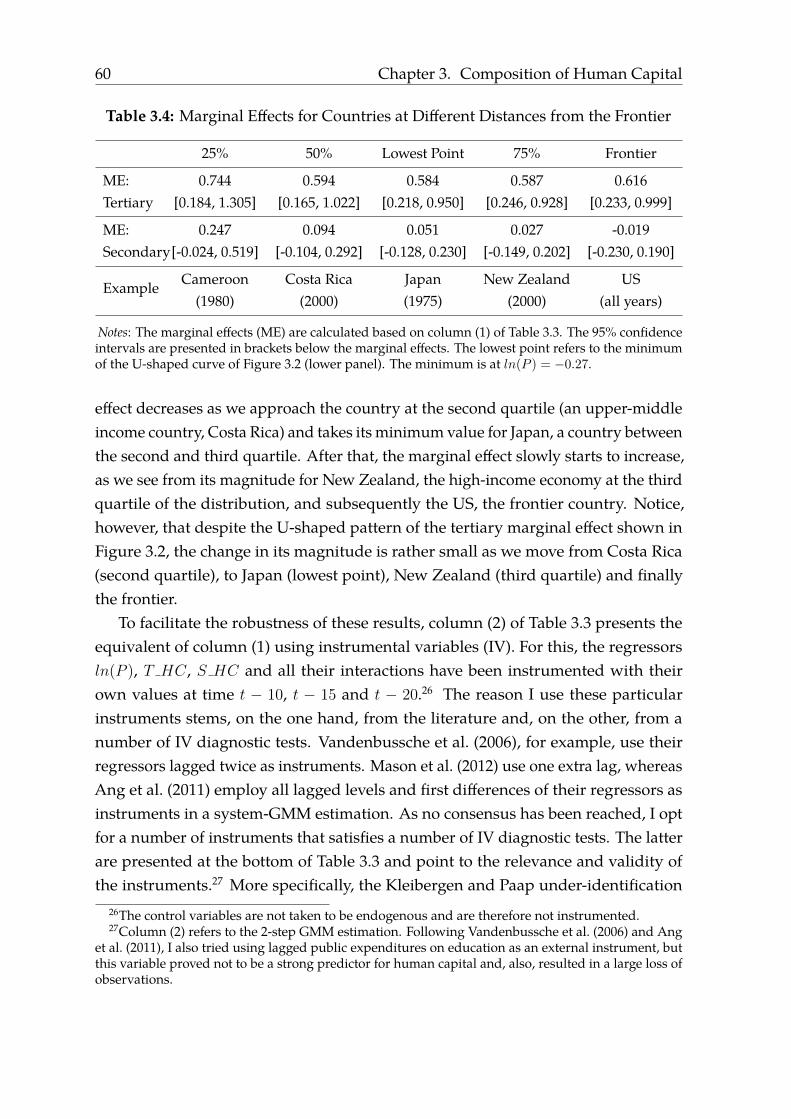
60 Chapter 3. Composition of Human Capital
Table 3.4: Marginal Effects for Countries at Different Distances from the Frontier
25% 50% Lowest Point 75% Frontier
ME: 0.744 0.594 0.584 0.587 0.616Tertiary [0.184, 1.305] [0.165, 1.022] [0.218, 0.950] [0.246, 0.928] [0.233, 0.999]
ME: 0.247 0.094 0.051 0.027 -0.019Secondary[-0.024, 0.519] [-0.104, 0.292] [-0.128, 0.230] [-0.149, 0.202] [-0.230, 0.190]
Example Cameroon Costa Rica Japan New Zealand US(1980) (2000) (1975) (2000) (all years)
Notes: The marginal effects (ME) are calculated based on column (1) of Table 3.3. The 95% confidenceintervals are presented in brackets below the marginal effects. The lowest point refers to the minimumof the U-shaped curve of Figure 3.2 (lower panel). The minimum is at ln(P ) = −0.27.
effect decreases as we approach the country at the second quartile (an upper-middleincome country, Costa Rica) and takes its minimum value for Japan, a country betweenthe second and third quartile. After that, the marginal effect slowly starts to increase,as we see from its magnitude for New Zealand, the high-income economy at the thirdquartile of the distribution, and subsequently the US, the frontier country. Notice,however, that despite the U-shaped pattern of the tertiary marginal effect shown inFigure 3.2, the change in its magnitude is rather small as we move from Costa Rica(second quartile), to Japan (lowest point), New Zealand (third quartile) and finallythe frontier.
To facilitate the robustness of these results, column (2) of Table 3.3 presents theequivalent of column (1) using instrumental variables (IV). For this, the regressorsln(P ), T HC, S HC and all their interactions have been instrumented with theirown values at time t − 10, t − 15 and t − 20.26 The reason I use these particularinstruments stems, on the one hand, from the literature and, on the other, from anumber of IV diagnostic tests. Vandenbussche et al. (2006), for example, use theirregressors lagged twice as instruments. Mason et al. (2012) use one extra lag, whereasAng et al. (2011) employ all lagged levels and first differences of their regressors asinstruments in a system-GMM estimation. As no consensus has been reached, I optfor a number of instruments that satisfies a number of IV diagnostic tests. The latterare presented at the bottom of Table 3.3 and point to the relevance and validity ofthe instruments.27 More specifically, the Kleibergen and Paap under-identification
26The control variables are not taken to be endogenous and are therefore not instrumented.27Column (2) refers to the 2-step GMM estimation. Following Vandenbussche et al. (2006) and Ang
et al. (2011), I also tried using lagged public expenditures on education as an external instrument, butthis variable proved not to be a strong predictor for human capital and, also, resulted in a large loss ofobservations.
Chapter 3. Composition of Human Capital 61
test rejects the null hypothesis that the equation is under-identified. According to theHansen J statistic, the instruments are valid. However, based on the endogeneity test, Icannot reject the null hypothesis that the specified endogenous regressors can actuallybe treated as exogenous in which case the OLS-FE estimates should be preferred.28 Forcompleteness, I present in Table 3.3 the results based on both estimation methods.29
To sum up, using different functional forms to identify the relationship betweenhuman capital and TFP growth, I have found robust evidence for externalities. Ter-tiary education, in particular, entails an overall positive effect on TFP growth whichdecreases as countries move closer to the frontier and, from a point onwards, increasesagain yet to a smaller extent. The decreasing impact is more dominant in my sampleand suggests a fundamental role of tertiary education for less developed economies,whereby high-skilled workers facilitate the adoption of technologies developed atthe frontier and promote growth. In these countries, tertiary human capital can alsoraise the productivity of the unskilled labor force, via “a higher incidence of learningfrom others” (Sianesi & van Reenen, 2003, p. 160). The increasing effect as countriesbecome more technologically advanced can be attributed to the fact that innovation,which requires a high-skilled labor force to materialize, is more pronounced, thanimitation, in countries close to the TFP frontier. Secondary education also results inexternalities, but smaller ones and significant only for a number of middle- and/orlow-income countries. Its effect does not increase when countries come closer to thefrontier.
3.4.4 Adjusted versus crude TFP
My results so far are based on what I call an adjusted TFP measure taken from PWT.As a final step, I would like to contrast these results with those based on a crudeproductivity measure, namely one that does not take into account the quality (educa-tional attainment) of the labor force. In this way, I will be able to conclude whether myresults are sensitive to the use of a TFP measure similar to that of Vandenbussche et al.(2006), Ang et al. (2011) and Cerina and Manca (2016). In order to do so, I re-calculatethe variables for TFP level and growth from PWT without adjusting for human capital,and re-do the analysis. The labor input into the production function is now merely thenumber of persons engaged in the economy. This implies that equations 3.4 and 3.6do not include the hc- but only the E-part of the labor input measure L.
28Note that the OLS-FE results were preferred over the IV ones in the specifications I estimated andthat held regardless of the functional form.
29Note that under the IV specification, observations drop and secondary education loses its signifi-cance among low- and lower-middle-income countries.

62 Chapter 3. Composition of Human Capital
Column (3) of Table 3.3 presents OLS-FE results based on the crude TFP measure.These can be directly compared to column (1) of the same table which uses the adjustedmeasure instead. Simply eyeballing the regression coefficients suggests that there isnot much difference between the two. The regressors carry the same sign and are ofsimilar magnitude. A test of the hypothesis that the coefficients of the two regressionsare equal, against the alternative that they are not, resulted in the rejection of thelatter.
Consequently, using an adjusted, instead of a crude, TFP measure does not alterthe core conclusions of my analysis. However, the former measure still has its meritsfor two reasons: first, conceptually, it is a better suited measure to use in the contextof externalities, as it allows for a distinction between private and social returns to edu-cation. Second, the TFP measures I adopt from the PWT allow for asset heterogeneityand labor shares to vary across countries and over time, which constitute importantimprovements in the construction of productivity data.
3.5 Conclusion
Human capital, commonly captured in empirical research by the level of education,holds a prominent role in academic and policy-related debates. In this paper, I haveexamined the relationship between different types of human capital and productivitygrowth for countries at different distances from the technology frontier, a topic whichhas produced mixed results in the literature. Motivated by the seminal work of Kruegerand Lindahl (2001) who found limited evidence of externalities, Vandenbussche etal. (2006) identified the importance of human capital composition and argued thata university-educated workforce is all the more important for innovating countries,close to the technology frontier. Ang et al. (2011) confirmed this finding for high- andmiddle-income countries but failed to find any externalities evidence for imitatingcountries, far from the technology frontier. In contrast to Vandenbussche et al. (2006)and using industry- rather than country-level analyses, Inklaar et al. (2008) and Masonet al. (2012) found no compelling externalities evidence. In contrast to Ang et al.(2011), Cerina and Manca (2016) pointed to the importance of high-skilled workersfor developing countries.
In this paper, I have employed different functional forms and used state-of-the-artTFP measures to examine the link between education and growth. My analysis hasdiscovered evidence of externalities that extends to all countries of my sample. Thecomposition of human capital matters greatly as it is primarily the tertiary-educated

Chapter 3. Composition of Human Capital 63
workers that contribute to growth. There is also evidence that the marginal effect oftertiary education on TFP growth is U-shaped: large for countries far from the tech-nology frontier and decreasing as we move closer to it, in line with Cerina and Manca(2016), but increasing as we further approach the frontier, in line with Vandenbusscheet al. (2006). It is worth noting, however, that the decreasing effect dominates and thattertiary education is found to play a fundamental role for growth, particularly for lesstechnologically advanced economies. The increase in the marginal effect for countriesclose to the frontier is relatively small in magnitude. All in all, investing in highereducation appears to generate social returns in all countries, poor and rich.

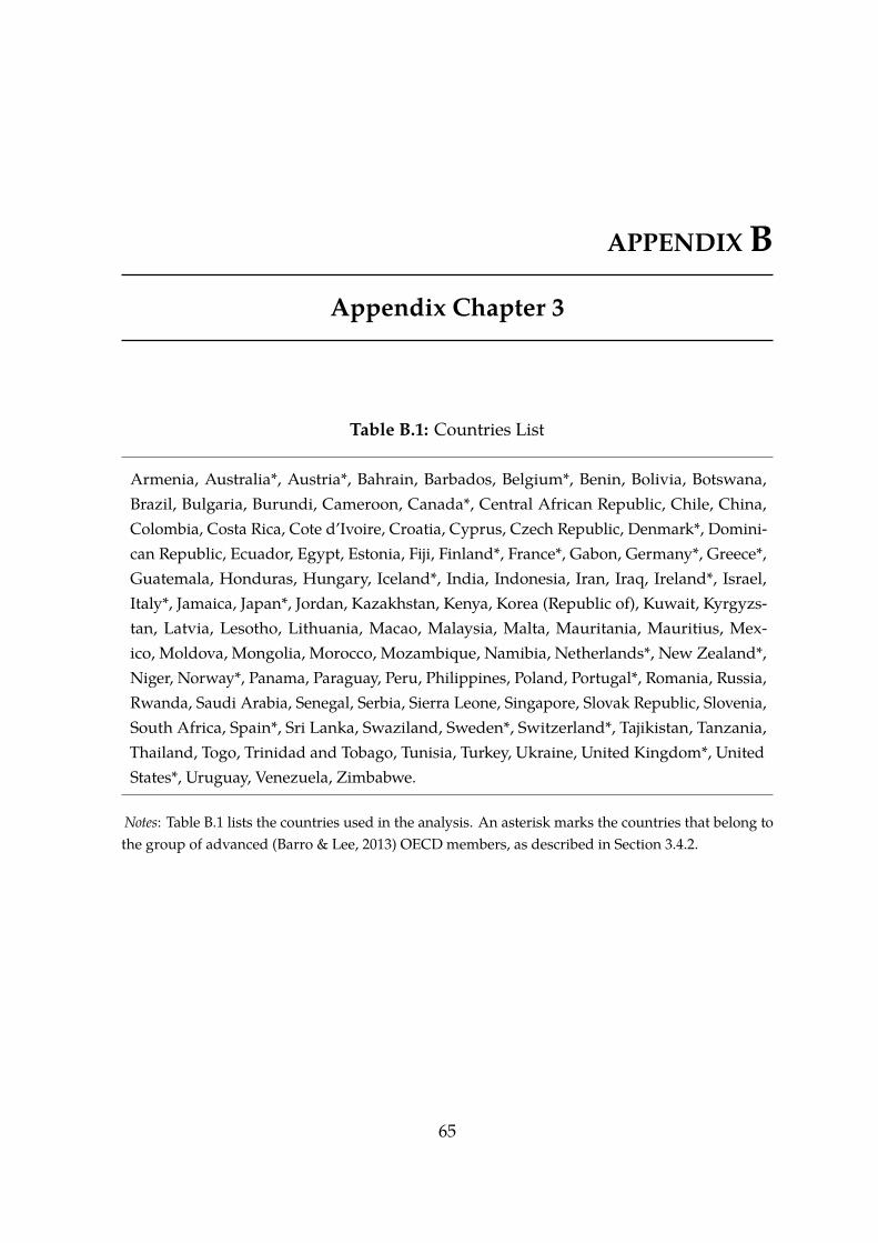
APPENDIX B
Appendix Chapter 3
Table B.1: Countries List
Armenia, Australia*, Austria*, Bahrain, Barbados, Belgium*, Benin, Bolivia, Botswana,Brazil, Bulgaria, Burundi, Cameroon, Canada*, Central African Republic, Chile, China,Colombia, Costa Rica, Cote d’Ivoire, Croatia, Cyprus, Czech Republic, Denmark*, Domini-can Republic, Ecuador, Egypt, Estonia, Fiji, Finland*, France*, Gabon, Germany*, Greece*,Guatemala, Honduras, Hungary, Iceland*, India, Indonesia, Iran, Iraq, Ireland*, Israel,Italy*, Jamaica, Japan*, Jordan, Kazakhstan, Kenya, Korea (Republic of), Kuwait, Kyrgyzs-tan, Latvia, Lesotho, Lithuania, Macao, Malaysia, Malta, Mauritania, Mauritius, Mex-ico, Moldova, Mongolia, Morocco, Mozambique, Namibia, Netherlands*, New Zealand*,Niger, Norway*, Panama, Paraguay, Peru, Philippines, Poland, Portugal*, Romania, Russia,Rwanda, Saudi Arabia, Senegal, Serbia, Sierra Leone, Singapore, Slovak Republic, Slovenia,South Africa, Spain*, Sri Lanka, Swaziland, Sweden*, Switzerland*, Tajikistan, Tanzania,Thailand, Togo, Trinidad and Tobago, Tunisia, Turkey, Ukraine, United Kingdom*, UnitedStates*, Uruguay, Venezuela, Zimbabwe.
Notes: Table B.1 lists the countries used in the analysis. An asterisk marks the countries that belong tothe group of advanced (Barro & Lee, 2013) OECD members, as described in Section 3.4.2.
65
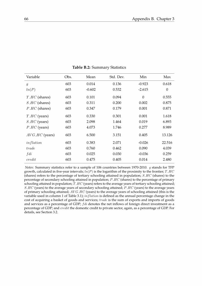
66 Appendix B. Chapter 3
Table B.2: Summary Statistics
Variable Obs. Mean Std. Dev. Min Max
g 603 0.014 0.136 -0.923 0.618ln(P ) 603 -0.602 0.532 -2.615 0
T HC (shares) 603 0.101 0.094 0 0.555S HC (shares) 603 0.311 0.200 0.002 0.875P HC (shares) 603 0.347 0.179 0.001 0.871
T HC (years) 603 0.330 0.301 0.001 1.618S HC (years) 603 2.098 1.464 0.019 6.893P HC (years) 603 4.073 1.746 0.277 8.989
AV G HC (years) 603 6.500 3.151 0.405 13.126
inflation 603 0.383 2.071 -0.026 22.516trade 603 0.760 0.462 0.090 4.039fdi 603 0.025 0.030 -0.036 0.259credit 603 0.475 0.405 0.014 2.480
Notes: Summary statistics refer to a sample of 106 countries between 1970-2010. g stands for TFPgrowth, calculated in five-year intervals; ln(P ) is the logarithm of the proximity to the frontier; T HC(shares) refers to the percentage of tertiary schooling attained in population; S HC (shares) to thepercentage of secondary schooling attained in population; P HC (shares) to the percentage of primaryschooling attained in population; T HC (years) refers to the average years of tertiary schooling attained;S HC (years) to the average years of secondary schooling attained; P HC (years) to the average yearsof primary schooling attained; AV G HC (years) to the average years of schooling attained (this is thevariable used in column 1 of Table 3.1); inflation is defined as the annual percentage change in thecost of acquiring a basket of goods and services; trade is the sum of exports and imports of goodsand services as a percentage of GDP; fdi denotes the net inflows of foreign direct investment as apercentage of GDP; and credit the domestic credit to private sector, again, as a percentage of GDP. Fordetails, see Section 3.2.

CHAPTER 4
Brain Drain or Gain? The Structure of Production,Emigration and Growth∗
4.1 Introduction
High-skilled people tend to emigrate from poorer countries in greater numbersthan the low-skilled, raising the specter of a ‘brain drain’ that would leave these
countries with less human capital and worse prospects for development.1 Docquierand Rapoport (2012, p. 682), for example, report that high-skilled migration fromdeveloping to developed economies increased faster compared to that of overallmigration towards OECD countries.2 However, the opportunity to migrate increasesthe expected returns to education, thus improving the incentives for human capitalformation and opening up the possibility of a ‘brain gain’.
To determine which of these effects is more important, the existing literature onmigration and human capital has typically tested whether larger high-skilled (i.e.university-educated) emigration leads to an increase in the number of high-skilledpeople, and found qualified support for this.3 More specifically, this direct approachimplies examining the effect high-skilled emigration rates have on human capitalaccumulation, captured by the growth in the proportion of high-skilled people inthe native population. One important drawback of this direct approach, though, is
∗For an earlier version of this chapter, see: Papakonstantinou and Inklaar (2014). We would like tothank Viola Angelini, Sorin Krammer, Marcel Timmer and seminar participants at the University ofGroningen for helpful comments and suggestions.
1See Bhagwati and Hamada (1974) for early discussions and Docquier and Rapoport (2012) for arecent overview of this topic. This paper focuses on the migration-human-capital relationship, butmigration has a broader range of effects on a country than just on the available amount of humancapital.
2With high-skilled migrants, the authors mean tertiary-educated ones.3See e.g. Beine, Docquier, and Rapoport (2001); Beine et al. (2008); Beine, Docquier, and Rapoport
(2010); Beine et al. (2011) and Di Maria and Lazarova (2012).
67

68 Chapter 4. Brain Drain or Gain?
that it ignores the impact on medium-skill levels,4 while these can also be importantfor increasing a country’s human capital. Another drawback is that positive effectsthat are farther removed in time are not attributed to the initial spur of migration.For instance, skill-biased technical change (SBTC) may increase demand for humancapital after the initial ‘brain gain’.
The contribution of our paper is to use a more indirect approach to test the rela-tionship between migration and human capital, so that we need not specify preciselywhich types of migration lead to which type of human capital improvement and howfast.5 We start from the empirical approach of Ciccone and Papaioannou (2009), whofind that a large initial human capital endowment leads to specialization in human-capital-intensive industries.6 We call this the education effect. After controlling for it,we find that countries with higher emigration rates also specialize in human-capital-intensive industries. We take this as evidence that countries with higher emigrationrates increase their endowment of human capital at a faster rate than countries withlower emigration rates. This migration effect is also economically important as it isabout one- to two-thirds as large as the education effect of Ciccone and Papaioannou(2009). Further analysis shows that the set of countries with the lowest initial levels ofhuman capital benefits even more from migration, a finding that is supportive of ourhypothesis and in line with the broader migration-human-capital literature. We alsoshow that our findings for total migration can be traced to the migration of the high-and medium-skilled, with no positive effect from low-skilled migration. This meansthat our effect is not driven by the emigration of low-skilled people, which wouldalso have raised average human capital levels, but instead points to the importance ofimproved incentives for human capital formation, i.e. a ‘brain gain’.
Our sample covers up to 68 countries and 28 manufacturing industries and weanalyze growth over the period 1980-2000. We employ a country-industry panelset-up, where we explain industry growth in value added or employment with aninteraction of a country’s emigration rate with an industry’s knowledge intensity.7
An important advantage of this approach is that reverse causality is less likely to be aproblem, since we identify the net migration effect from the variation in growth across
4People that finish upper-secondary but not tertiary education.5That indirectness is also a drawback, since those detailed links of the causal chain are important
to establish which aspects of the relationship are important, when and where. We feel this is a priceworth paying in that our indirect approach opens up new avenues for research.
6Romalis (2004) has shown similar results in the context of trade specialization.7As well as country and industry fixed effects and a range of control variables.
Chapter 4. Brain Drain or Gain? 69
industries within countries.8 In contrast, most of the empirical studies on ‘brain drain’have relied on cross-sectional samples, which limits the ability to draw ”conclusiveinferences regarding causality” (Di Maria & Lazarova, 2012, p. 942).
Our findings are robust to using value added or employment growth as dependentvariables; to different measures of industries’ knowledge intensity; to the use ofdifferent migration databases; and to measurement error in the migration data. Wealso show that our findings do not simply reflect that more open economies specializein more knowledge-intensive activities. When we include alternative indicators ofopenness, such as openness to migratory inflows, trade and foreign direct investment(FDI), the effect of emigration on growth of knowledge-intensive industries is verysimilar.
Our paper proceeds as follows: Section 4.2 discusses the related literature. Section4.3 introduces the empirical model, Section 4.4 presents the data and Section 4.5 theresults. Section 4.6 puts forward points for discussion and Section 4.7 concludes.
4.2 Related Literature
Determining the effect of emigration on human capital is very relevant in view ofhuman capital as a key determinant of economic growth. In this section we brieflydiscuss the literature, though we refer the reader to Docquier and Rapoport (2012) fora more extensive review of the ‘brain drain/gain’ debate.
International migration entails welfare implications and affects the economic per-formance of the sending country (Chen, 2009). More specifically, high-skilled emigra-tion has a direct negative effect on the level of human capital as it deprives the homecountry of its high-skilled workforce, i.e. a ‘brain drain’ occurs. The economy not onlyloses workers that could be employed in the domestic production, but, partly, also itscapacity to innovate and/or adopt new technologies (Marchiori, Shen, & Docquier,2013). However, the literature identifies various feedback mechanisms through which(high-skilled) emigration could lead to increases in human capital, potentially bene-fiting the source economy and giving rise to a ‘brain gain’. These feedback channelsinclude remittances (Faini, 2007; Adams & Cuecuecha, 2013), return migration (Borjas,1989; Faini, 2003) and technology diffusion via scientific networks formed by migrants(Kerr, 2008).
Furthermore, emigration improves the incentives to acquire (or upgrade one’s)8See also Rajan and Zingales (1998) on the relationship between financial development and growth.
Using international patent citations, Kerr (2008) employs a similar approach to show how ethnicresearch communities in the US affect technology diffusion.

70 Chapter 4. Brain Drain or Gain?
skills: if the opportunity to migrate improves the expected returns to education, theincentives to actually get an education improve, potentially leading to a ‘brain gain’.Given that only part of a country’s residents will eventually emigrate, the level ofhuman capital need not decrease but could even increase with greater emigration.Mountford (1997) and Stark et al. (1997, 1998) were the first to theoretically establishthe ‘brain gain’ argument based on the idea that “expectations about future migrationopportunities affect education decisions” (Docquier & Rapoport, 2012, p. 701).
The greater availability of migration data has also triggered empirical research,at the macro-level (Beine et al., 2001; Faini, 2003; Beine et al., 2008; Docquier et al.,2008; Beine et al., 2010, 2011; Di Maria & Lazarova, 2012) and the micro-level (Gibson& McKenzie, 2011; Batista et al., 2012), to establish whether there is indeed an incen-tive effect, i.e. whether greater emigration opportunities lead to more schooling.9
Although there is growing evidence in favor of the ‘brain gain’, there are still con-tradictory findings in the literature and the debate is far from settled. In the nextsections, we turn to our approach to study the ‘brain drain/gain’.
4.3 The Model
Our model to estimate the effect of emigration on growth of knowledge-intensiveindustries draws on the work of Ciccone and Papaioannou (2009) and takes thefollowing form:
gs,i = β1 · (Ms/Ps) ·KIi + β2 ·HCs ·KIi + β3 ·X ′i · Zs + β4 · Ss,i + λs + µi + εs,i (4.1)
where the dependent variable is the annual growth rate g of value added oremployment in country of origin s in industry i during the 1980-2000 period; Ms/Ps
is the ratio of the number of people that lived abroad to a country’s population in1980; KIi is the knowledge intensity of industry i; HCs is an indicator of the levelof human capital in 1980 in country s and Ss,i denotes the share of industry i inmanufacturing value added or employment of country s in the beginning of theperiod. The inclusion of this variable allows us to control for initial differences in thesize of various industries. We also control for other determinants of industry growth(physical capital, property rights and financial development) by interacting a countrylevel variable (Zs) with an industry level variable (Xi). Finally, λs and µi are country-
9This stream of (empirical macro) research is discussed in more detail in Section 4.6 where wecompare our findings to those of the existing literature.

Chapter 4. Brain Drain or Gain? 71
and industry-specific effects and residual growth is captured by εs,i. The inclusionof country and industry effects means that we are comparing differential industrygrowth patterns within countries.
Compared with Ciccone and Papaioannou (2009), our model adds the migrationterm, (Ms/Ps) ·KIi. Ciccone and Papaioannou (2009) find that β2 is positive: a higherinitial endowment of human capital leads to faster growth of knowledge-intensiveindustries. We focus on β1, so whether migration has an effect on the growth ofknowledge-intensive industries after the effect of the initial endowment of humancapital has been accounted for. If there is a significant and positive effect, we take thisas evidence that high-migration countries have increased their human capital at afaster rate than low-migration countries. This would correspond to a net ‘brain gain’,while a negative β1 would imply a net ‘brain drain’.
The model we use is an indirect method of identifying the effect of migrationon human capital: we interpret a relationship between migration and the growthof knowledge-intensive industries as being driven by changes in human capital. Anadvantage of this indirect approach is that we do not need to precisely identify eachlink of the causal chain -from emigration of certain types of workers, to improvedincentives for others to increase their human capital, to a particular net effect on totalhuman capital. Instead, we simply note that to explain the observed growth patternin high-emigration countries, human capital has to have changed in a particulardirection. That does require carefully controlling for the initial human capital level,which we do following Ciccone and Papaioannou (2009). It also requires ascertainingthat the emigration rate is not a proxy for a more general type of openness: if theeconomy is more open, it might more easily attract foreign investment and technology,stimulating growth in precisely the knowledge-intensive industries. We also do thisin our analysis.
One other concern could be that we analyze the effect of total migration, ratherthan migration by skill type. This means that, say, a positive β1 could be the result ofpredominantly skilled emigration leading to stronger incentives to get an education(i.e. the ‘brain gain’ argument) but it could also be the result of unskilled emigrationthat directly raises the average level of human capital of the origin country. Given theimportance of skilled emigration, the ‘brain gain’ argument seems the most relevantone a priori, but to explicitly distinguish between these explanations we also splitoverall emigration into emigration by skill type.
72 Chapter 4. Brain Drain or Gain?
4.4 Data
4.4.1 Industry growth
The dependent variable of our model (gs,i) is the compound annual growth rate ofvalue added or employment and refers to the country of origin s and the industry i overthe 1980-2000 period.10 Data on both value added and employment are obtained fromthe Industrial Statistics of the United Nations Industrial Development Organization(UNIDO, 2006). The 2006 edition of the INDSTAT3 database reports value addedand employment data for 181 countries and 28 manufacturing industries (as wellas for total manufacturing) for the period 1963 to 2004, organized at the three-digitInternational Standard Industrial Classification (ISIC) revision 2 level.
For a country to be included in our study, we first require that the UNIDO (2006)dataset has value added (or employment) information for it for at least ten years. Weset 1980 as the first and 2000 as the last year to derive data for our analysis. We do so,as the knowledge intensity variable we use (KIi) refers to the year 1980 and also, inorder to allow for long-term effects of emigration on industry growth. If, however,the country-industry-specific value added (or employment) data are missing in 1980and/or 2000 (or are zero or negative -the latter occurs in value added data but notoften), we respectively use the value of the first available year after 1980 and/or before2000 instead. We do so to allow for a broader sample of countries and industriesin our analysis, as the country-industry coverage in UNIDO (2006) varies over theyears (for example, more information is available for the 1980s compared to the 1990s).The number of years between the first and last observation is taken into accountthrough the compound annual growth rate calculation. Furthermore, we require adifference of at least ten years between the first and the last observation, again inorder to examine relatively long-term effects. Following Ciccone and Papaioannou(2009), for a country-industry observation to be included in the analysis, it shouldrefer to a year (between 1980 and 2000) that has (non-missing) observations for at leastten industries. The data to construct our initial share (Ss,i) variable are also derivedfrom UNIDO (2006). This variable is the ratio of value added (or employment) of aparticular country and industry, in the first year for which data are available, to the
10Growth is computed as the compound annual growth rate (CAGR): (YT /Yt)1/T−t − 1 where YT is
value added or employment in year T (the year for which value added or employment is last observed,but not after 2000) and Yt is value added or employment in year t (the year for which value added oremployment is first observed, but not before 1980). Y refers to country-industry-specific observations.We allow for a difference (T − t) of no less than ten (and a maximum of twenty) in order to capturerelatively long-term effects. See the main text for a detailed discussion of the variables construction.
Chapter 4. Brain Drain or Gain? 73
total manufacturing value added (or employment) of the country in that same year.Important to note at this point is that, in the UNIDO (2006) dataset, value added is
expressed in current US dollars.11 In order to appropriately deflate value added, onewould need a country-industry-specific deflator, which is however largely unavailablefor all countries and industries included in our analysis. Deflating the data using forexample the US producer price index would still not take into account the country-industry specific inflation effect, controlling for which is rather unclear if and to whatextent and direction would affect our results. For that reason, we also conduct theanalysis using employment data, following Ciccone and Papaioannou (2009).
Our data are limited to the manufacturing sector of the economy, primarily forreasons of data availability. Furthermore, manufacturing industries may be drivenmore strongly by country-level supply-side factors (e.g. the endowment of humancapital) than by country-level demand factors. Since manufacturing industries tendto sell their products not only domestically but also abroad, country-specific demandfactors favoring one set of industries over another are less likely to play a dominantrole. Since we are interested in identifying the effect of human capital, a supply-sidefactor, our manufacturing data can be helpful. In addition, manufacturing industriesare not qualitatively different from other industries in terms of knowledge intensity.Both manufacturing and non-manufacturing industries can have a low knowledgeintensity (e.g. wood products and construction) or a high knowledge intensity (e.g.electronics and financial services).
Following the literature that employs country-industry specifications (for example,Rajan & Zingales, 1998; Ciccone & Papaioannou, 2009), we exclude the United Statesfrom the sample since it acts as our benchmark country. A maximum of 66 countriesis included in our regressions using value added and 68 in our employment specifica-tions. A list of all countries included in the analysis can be found in Table C.1 of theappendix.
4.4.2 Knowledge intensity
Our empirical specification requires data on the knowledge intensity of manufactur-ing industries. Since information at the industry level is rather limited, we followthe literature that employs country-industry models (Rajan & Zingales, 1998; Cic-cone & Papaioannou, 2009) and rely on data from a benchmark country to proxyglobal industry characteristics. The United States has been suggested as a natural
11As stated in the data documentation file, “data are originally stored in national currency values atcurrent prices. The system allows conversion of currency data from national currency into current USdollars, using the average period exchange rates” (UNIDO, 2006).

74 Chapter 4. Brain Drain or Gain?
choice, partly because US data are detailed, reliable and widely available, but alsobecause US labor markets are less regulated (Ciccone & Papaioannou, 2009, p. 70).Therefore, inter-industry knowledge intensity differences are likely to better captureinter-industry technological differences. Since there is a technological reason whysome industries have higher levels of knowledge intensity than others, we expectinter-industry technological differences to persist across countries. We are thereforeconfident that using the US as a benchmark yields good proxies for global industrycharacteristics. We are not claiming here that it is necessary for industries to experi-ence the same absolute level of knowledge intensity across all countries as there arelarge differences in the magnitude of knowledge intensity across countries. Instead,we require a statement of the following type to hold: “If petroleum refineries requirea larger level of knowledge intensity than leather products in the United States, it willalso require a larger knowledge intensity level in India” (compare Rajan and Zingales(1998, p. 563)).
Data on the knowledge intensity of industries are from Ciccone and Papaioannou(2009). The authors compute three knowledge intensity measures for 28 US man-ufacturing industries in 1980: (i) the average years of schooling of employees (wecall this variable schoolingi), (ii) the ratio of hours worked by employees with at leasttwelve (secondaryi) and (iii) at least sixteen (collegei) years of schooling to total hoursworked by all employees. We use all three of them in the empirical analysis. The mostknowledge-intensive industries are petroleum refineries, printing and publishingand industrial and other chemicals, while the least knowledge-intensive are leatherproducts, wearing apparel, footwear and textiles.
4.4.3 Country data
The main variable of interest in our empirical specification is migration. We measuremigration as the number of people living away from their home country relative to thesending country’s population (Ms/Ps), both in 1980. This variable is interacted withthe industry level knowledge intensity variable (schoolingi, secondaryi or collegei) toform the main regressor of our analysis, the migration interaction, (Ms/Ps) · KIi.Migration data are from the Global Bilateral Migration Database (GBMD) (Ozden,Parsons, & Schiff, 2011) and population data from the World Development Indicators(WDI, 2012). The GBMD provides information on bilateral migrant stocks for 226countries. The figures are decennial and cover the period 1960-2000.12 We focus on the
12The figures come from censuses (therefore they are decennial) but, when observations are missing,they are generated either by interpolation or by applying propensity measures (see, Ozden et al. (2011)).
Chapter 4. Brain Drain or Gain? 75
year 1980, which constitutes the beginning of the period under examination and, sincethe data are in a bilateral set-up, we sum them by country of origin over all receivingcountries. Note that we thus use information on the stock of migrants. This is ameasure that is consistent with our analysis since it not only includes individuals wholeave the home country in 1980 but also those that left in earlier years. Data for totalmigration (based on Ozden et al. (2011)) and total population (based on WDI (2012))are presented in Table C.1 of the appendix (columns (2) and (6) respectively). Theratio of the two, which is the variable that, interacted with knowledge intensity, entersthe regressions, reveals that the countries included in our benchmark specificationhave on average 5.8% of their population living abroad. The smallest share is that ofBrazil (0.25%), while Jordan has the largest ratio of migration to population amongour set of countries (28.8%).
We use the GBMD (Ozden et al., 2011) for our analysis because, first, it includesinformation for the year 1980, the beginning of the period under examination, and,second, because it captures migration towards the whole world, rather than onlytowards OECD (Organisation for Economic Co-operation and Development) countriesas the bulk of studies on ‘brain drain’ (Beine et al., 2001, 2008, 2010, 2011; Di Maria& Lazarova, 2012). However, to facilitate the robustness of our results, we later alsouse alternative migration databases (Dumont, Spielvogel, & Widmaier, 2010; UnitedNations Department of Economic and Social Affairs, 2012; Brucker, Capuano, &Marfouk, 2013). Our findings are broadly similar (see, Section 4.5.3).
We are also interested in controlling for the direct effect of human capital on growthof knowledge-intensive industries, to capture the effect that Ciccone and Papaioannou(2009) focus on. We use three different measures of human capital in 1980, takenfrom the Barro and Lee dataset on educational attainment (Barro & Lee, 2013, version1.2): (i) average years of schooling (yr schs in Barro and Lee (2013)), (ii) percentage ofcomplete secondary (lscs) and (iii) percentage of complete tertiary (lhcs) schoolingattained in a country’s population. We interact the industry level variable schoolingiwith the country level variable yr schs, secondaryi with lscs and collegei with lhcs andthese form the human capital interaction variable.
Following the approach of Ciccone and Papaioannou (2009), we include othervariables that may affect the specialization patterns of countries. These variables alsotake the form of industry characteristics interacted with country characteristics. Again,industry level variables refer to our benchmark country, namely the US.
We use industry capital intensity (ki) interacted with country capital levels (Ks/Ys)to control for the effect that a greater endowment of capital could lead to a specializa-tion in more capital-intensive industries (following Romalis (2004)). We also interact

76 Chapter 4. Brain Drain or Gain?
an industry’s contract intensity (ci) with a country’s property rights index (Ps), anapproach also followed by Nunn (2007) and Chor (2010). In our specifications, Psinteracted with ci shows whether countries with good property rights specialize incontract-intensive industries. Finally, we interact an industry’s dependence on ex-ternal finance (edi) with a country’s level of financial development (FDs). With thisinteraction, we are able to control for the Rajan and Zingales’ (1998) argument thatexternal finance dependent industries experience faster growth in countries with ahigher level of financial development.
To ensure that the migration effect not only reflects a general impact of openness onindustrial specialization, we also consider a number of control variables that capturedifferent aspects of openness. Specifically, we consider the number of immigrants tothe total population (IMs/Ps), the ratio of exports to GDP (Xs), the ratio of exports plusimports to GDP (XMs) and the ratio of FDI to GDP (FDIs). Each of these variables isalso interacted with industry knowledge intensity (KIi) to establish whether opennessleads to faster growth in knowledge-intensive industries. If the (e)migration variableonly measures the general degree of openness of the economy, we would expect itscoefficient to fall substantially as other measures of openness are included. If insteadthe coefficient on migration captures an additional effect, i.e. the incentive effect foundelsewhere in the literature, the coefficient would not be much affected by the inclusionof alternative openness measures. Table C.2 of the appendix summarizes the fulldefinition and sources for all variables used in the analysis.
4.5 Results
In this section, we first explore whether countries that have higher emigration sub-sequently experience faster growth in knowledge-intensive industries. Second, weconsider whether the effect differs across countries. Third, we decompose migrantsby their skill/education level and, fourth, we put our analysis through a number ofrobustness tests.
4.5.1 Initial migration shares and subsequent industry growth
Table 4.1 presents our results when growth in value added (columns (1), (2), (3)) andgrowth in employment (columns (4), (5), (6)) serve as the dependent variable of ourmodel. The first row (Total Migration ·KIi) reports the effect of initial migrationon growth of knowledge-intensive industries (the β1-coefficient). All specificationsincorporate the control variables for the level of human capital, physical capital,

Chapter 4. Brain Drain or Gain? 77
property rights, financial development and the initial share of each industry in totalmanufacturing. Columns (1) and (4) use the industry level variable schooling tomeasure industry knowledge intensity, columns (2) and (5) use secondary and columns(3) and (6) use college.
We see that the coefficient for the migration interaction is positive and statisticallysignificant at the 5% or 1% level across all specifications, with the exception of column(4) of Table 4.1 where it turns marginally insignificant (p=0.108).13 In other words,countries with higher emigration rates show faster subsequent growth in knowledge-intensive manufacturing industries. This implies that better emigration prospectsimprove the level of human capital. Given the importance of skilled migration thiscould well be evidence for the ‘brain gain’ argument, where better opportunities toemigrate improve the incentives to get an education. This improvement in incentiveswould then outweigh the actual ‘brain drain’ from skilled workers leaving the country.Our results remain robust when we use both value added and employment growth,as well as to the inclusion of control variables and different measures of industries’knowledge intensity.
From the table we see that the human capital interaction also shows positive andstatistically significant coefficients across all specifications, in line with Ciccone andPapaioannou (2009). This implies that the effect of migration on industry growthoperates in addition to the effect of initial human capital. This in turn implies thathigher emigration would lead to increases in human capital from a given initial level.
To get a sense of the size of the estimates, consider an industry with a high knowl-edge intensity (e.g. transport equipment) and one with a low knowledge intensity (e.g.pottery); a country with a high emigration share (e.g. Mauritius) and one with a lowemigration share (e.g. Philippines) and also a country with high human capital levels(e.g. Denmark) and one with low human capital levels (e.g. Zimbabwe). When weexamine growth in value added, our findings for the migration effect imply that thetransport equipment industry grows 0.28 to 0.32 percentage points faster (on averageper year) than the pottery industry when comparing growth in Mauritius to the Philip-pines. In comparison, the education effect shows that transport equipment grows0.46 to 0.73 percentage points faster in Denmark than in Zimbabwe. The estimatedemployment regressions imply similar effects, with a migration effect of 0.22 to 0.27percentage points and an education effect of 0.47 to 0.94 percentage points.14
Note further that the physical capital interaction variable is always positive but
13Note that when we use past values of migration as an instrument to alleviate measurement error,migration becomes significant, at the 5% level (see also Table 4.5 and the discussion below).
14These calculations are based on the results of all columns of Table 4.1.

78 Chapter 4. Brain Drain or Gain?
Tabl
e4.
1:Th
eEff
ecto
fMig
ratio
non
Gro
wth
ofVa
lue
Add
edan
dEm
ploy
men
t
VARI
ABL
ESVa
lue
Add
edEm
ploy
men
t(1
:sch
.)(2
:sec
.)(3
:coll.)
(4:sch
.)(5
:sec
.)(6
:coll.)
Tota
lMig
ratio
n·KI i
0.05
75**
0.44
9**
1.04
9***
0.04
360.
417*
*0.
737*
*(0
.021
7)(0
.171
)(0
.311
)(0
.026
8)(0
.202
)(0
.369
)H
uman
Cap
ital·KI i
0.00
175*
*0.
348*
*1.
586*
**0.
0022
2**
0.46
5**
1.80
7***
(0.0
0081
7)(0
.154
)(0
.573
)(0
.000
907)
(0.1
90)
(0.6
41)
Phys
ical
Cap
ital·ki
0.00
264
0.00
262
0.00
350
0.00
288
0.00
276
0.00
405
(0.0
0466
)(0
.004
68)
(0.0
0462
)(0
.004
22)
(0.0
0430
)(0
.004
24)
Prop
erty
Righ
ts·ci
-0.0
0567
-0.0
0581
-0.0
0562
-0.0
0613
-0.0
0631
-0.0
0610
(0.0
0593
)(0
.005
97)
(0.0
0589
)(0
.004
54)
(0.0
0459
)(0
.004
52)
Fina
ncia
lDev
elop
men
t·edi
0.03
69**
0.03
67*
0.04
05**
0.03
44**
0.03
38**
0.03
92**
(0.0
182)
(0.0
185)
(0.0
184)
(0.0
153)
(0.0
155)
(0.0
160)
Initi
alSh
are
-0.2
16**
*-0
.213
***
-0.2
10**
*-0
.174
***
-0.1
71**
*-0
.163
***
(0.0
540)
(0.0
540)
(0.0
539)
(0.0
397)
(0.0
406)
(0.0
386)
Obs
erva
tions
1,66
81,
668
1,66
81,
733
1,73
31,
733
Cou
ntri
es66
6666
6868
68R-
squa
red
0.13
40.
132
0.13
40.
135
0.13
30.
132
Not
es:T
able
4.1
pres
ents
the
resu
ltsw
ithgr
owth
inva
lue
adde
d(c
olum
ns(1
)-(3)
)and
empl
oym
ent(
colu
mns
(4)-(
6)).
Mig
ratio
nda
taar
efr
omth
eG
BMD
(Ozd
enet
al.,
2011
).C
olum
ns(1
)and
(4)u
seth
ein
dust
ryle
velv
aria
bleschooling
tom
easu
rein
dust
rykn
owle
dge
inte
nsity
,col
umns
(2)a
nd(5
)the
vari
ablesecondary
and
colu
mns
(3)a
nd(6
)the
college
one.
See
Tabl
eC
.2fo
rvar
iabl
ede
finiti
ons.
All
spec
ifica
tions
incl
ude
coun
try
and
indu
stry
fixed
effec
ts.R
obus
tsta
ndar
der
rors
,clu
ster
edby
coun
try,
inpa
rent
hese
s,**
*p<
0.01
,**p<
0.05
,*p<
0.1.

Chapter 4. Brain Drain or Gain? 79
never statistically significant, in line with the estimates of Ciccone and Papaioannou(2009). Second, the property rights interaction enters with a negative sign, althoughalways insignificant. Intuitively, we would expect to find a positive coefficient for thisvariable, since literature suggests that countries with better institutions specializein the more complex industries (Costinot, 2009). However, the exclusion of thisvariable did not alter our results. Furthermore, using other data sources (for example,the International Country Risk Guide Project and the Freedom House) to measureproperty rights did not affect our estimates. We opted for data from the Fraser Institute(Gwartney, Lawson, & Hall, 2012) since they cover the largest possible number ofcountries and the data are publicly available and widely used. Additionally, thecountry level variable we derive from Fraser Institute reflects the legal system andsecurity of property rights and we believe that it matches better with contract intensity,the respective industry level variable, than, for example, a variable that measures civilliberties or political rights. Third, the finance interaction always enters with a positiveand statistically significant sign (at the 10% or 5% level), in line with the results ofRajan and Zingales (1998). Finally, as was to be expected, the variable that controlsfor initial differences in the size of various industries (Initial Share, Ss,i) always has anegative and highly statistically significant coefficient.
4.5.2 Heterogeneity across countries
As a next step, we want to explore whether the ‘brain gain’ effect that we find is morepronounced in some countries rather than others. We find evidence that the countrieswith the lowest levels of human capital benefit the most from emigration, based onthe following equation:
gs,i = β1 · (Ms/Ps) ·KIi + β5 · (Ms/Ps) ·KIi · Hs + β2 ·HCs ·KIi+
β3 ·X ′i · Zs + β4 · Ss,i + λs + µi + εs,i(4.2)
In this equation we include an extra term, where the migration interaction isfurther interacted with the dummy variable Hs. This dummy variable equals one forcountries in the bottom quartile of the world human-capital distribution (lhcs < 0.0074)as identified from all countries included in Barro and Lee (2013).15 Coefficient β1now gives the effect of migration on growth of knowledge-intensive industries incountries in the top three quartiles of the human-capital distribution, while β5 shows
15We experimented with alternative cut-off points and continuous interactions. These did not revealclear patterns.

80 Chapter 4. Brain Drain or Gain?
Table 4.2: The Effect of Migration and the Initial Level of Human Capital
VARIABLES Value Added Employment(1) (2)
Total Migration ·KIi 1.206*** 0.891**(0.301) (0.354)
Total Migration ·KIi · Hs 7.827** 7.802**(3.402) (3.572)
Human Capital ·KIi 2.340*** 2.563***(0.605) (0.695)
Observations 1,668 1,733Countries 66 68R-squared 0.139 0.139
Notes: Table 4.2 presents the results with growth in value added (column (1)) and employment (column(2)). Migration data are from the GBMD (Ozden et al., 2011). In both cases, the industry level variablecollege is used. The human capital dummy (Hs) is equal to one for countries in the bottom quartile ofthe world human-capital distribution. See Table C.2 for variable definitions. All specifications includecountry and industry fixed effects, and also control for physical capital, property rights, financialdevelopment and the initial share (coefficients not reported). Robust standard errors, clustered bycountry, in parentheses, *** p<0.01, ** p<0.05, * p<0.1.
the additional impact of migration in countries in the bottom quartile.
The results in Table 4.2 show that the low human capital countries experience agreater shift in specialization towards more knowledge-intensive industries, comparedto countries with initially high levels of human capital. This can be explained from theidea that the lower quartile group of countries would more easily be able to increaseits human capital level from the initially low base. However, the countries with higherlevels of human capital still show significantly faster growth in knowledge-intensiveindustries, so in the analysis that follows, we use the results from Table 4.1 as ourbaseline.16 The results are only shown for the college measure, but are broadly similarfor the other knowledge-intensity measures.17 Note also that the specifications ofTable 4.2 incorporate all control variables (physical capital, property rights, financialdevelopment, initial share). The coefficients are not reported here, due to brevity, butare similar in magnitude and statistical significance to those reported in Table 4.1.
16Note that the coefficients from equation 4.2 are both larger than the migration effect in Table 4.1based on equation 4.1. This seems related to the inclusion of both country and industry dummies andthe resulting smaller within-country variation of the migration-human-capital interaction variable.Multicollinearity can then push up both coefficients.
17Due to brevity, in the rest of the paper, we only present the results with the knowledge intensityvariable college.

Chapter 4. Brain Drain or Gain? 81
4.5.3 Skill-decomposition of migrants
The purpose of this subsection is twofold: first, we want to test the robustness of ourfindings to the use of an alternative migration database. Second, we want to examinewhich skill-groups of migrants drive our results. So far, we have studied the effect oftotal migration on industrial specialization and found that it leads to faster growth ofknowledge-intensive industries. However, this effect could be systematically relatedto skilled emigration and improved incentives for human capital formation (i.e. ‘braingain’) or to unskilled emigration, which directly raises the average level of humancapital in a country. Distinguishing between these explanations requires a distinctionbetween the skilled and the unskilled migration rate.
Table 4.3 presents the results using the migration database of Brucker et al. (2013).Data refer to migration towards 20 OECD destination countries in the year 1980 (whilethe GBMD covers migration to all countries).18 One important advantage of thisdataset is that, particularly for the year 1980, information is not based on imputationsbut almost entirely directly from censuses or population registers of the destinationcountries.19 Columns (1) and (3) of Table 4.3 show the value added and employmentregression respectively. Both columns refer to the total stock of migrants (Bruckeret al., 2013) divided by the origin country’s population in 1980 (WDI, 2012) and tothe college variable to capture industry knowledge intensity. These columns showthat our earlier results, based on the GBMD (Ozden et al., 2011), also hold with thisalternative database.20
The main benefit of the Brucker et al. (2013) data is information on the skill compo-sition of migrants. In columns (2) and (4) of Table 4.3, we separate the total migrationrate into two groups, high- and medium-skilled migrants and low-skilled migrants.We combine the high- and medium-skilled in a single group, because migration ofthe two skill groups is so highly correlated (about 0.96) that separate effects cannot be
18The Brucker et al. (2013) dataset covers migration in the period 1980-2010 in five-years intervalsand refers to the total number of foreign-born individuals aged 25 and over living in each of thefollowing 20 OECD destination countries: Australia, Austria, Canada, Chile, Denmark, Finland, France,Germany, Greece, Ireland, Luxembourg, Netherlands, New Zealand, Norway, Portugal, Spain, Sweden,Switzerland, United Kingdom, and the United States.
19The Netherlands is the only exception.20We have also performed our analysis using data from Dumont et al. (2010) and the United Nations
Department of Economic and Social Affairs (2012). The migration variable was positive and significantat the 5% or 10% level for the case of value added and positive but insignificant for the case ofemployment using these datasets. We present the results using the Brucker et al. (2013) dataset since itrefers to the year 1980, the beginning of the period under examination. Data from Dumont et al. (2010)and the United Nations Department of Economic and Social Affairs (2012) refer to later years (1990and 2000).

82 Chapter 4. Brain Drain or Gain?
Table 4.3: Skill-decomposition of Migrants
VARIABLES Value Added Employment(1) (2) (3) (4)
Total Migration ·KIi 1.265*** 0.925*(0.384) (0.496)
High- and Medium-skilled Migration ·KIi 3.589*** 2.316*(0.901) (1.359)
Low-skilled Migration ·KIi -1.223 -0.581(0.948) (1.312)
Human Capital ·KIi 1.546** 1.420** 1.768*** 1.696**(0.585) (0.579) (0.644) (0.655)
Observations 1,668 1,668 1,733 1,733Countries 66 66 68 68R-squared 0.133 0.134 0.131 0.132
Notes: Table 4.3 presents the results with growth in value added (columns (1) and (2)) and employment(columns (3) and (4)). Migration data are from Brucker et al. (2013). In all cases, the industry levelvariable college is used. See Table C.2 for variable definitions. All specifications include country andindustry fixed effects, and also control for physical capital, property rights, financial development andthe initial share (coefficients not reported). Robust standard errors, clustered by country, in parentheses,*** p<0.01, ** p<0.05, * p<0.1.
identified.21
The group of high-skilled migrants have finished tertiary education, medium-skilled have secondary education and hold a high-school certificate and low-skilled arethose with lower-secondary, primary and no schooling attainment. We simultaneouslyintroduce in the regressions two variables: one that captures the share of high- andmedium-skilled migrants (Brucker et al., 2013) to a country’s population (WDI, 2012)in 1980 and one that refers to the ratio of low-skilled migrants (Brucker et al., 2013) topopulation (WDI, 2012) in that same year. In this way, we can contrast the coefficientsof these variables and determine whether the ‘brain gain’ argument holds or whetherour results are due to unskilled migration.
Table 4.3 shows the results for value added (column (2)) and employment growth(column (4)). The coefficient of high- and medium-skilled migration is positive andsignificant, whereas that of low-skilled migration is insignificant. This supportsthe ‘brain gain’ argument and shows that the high- and medium-skilled migrantsdrive the growth in human-capital-intensive industries. This suggests that migration
21Note that if we perform separate regressions, one for the high- and one for the medium-skilledmigration, we still conclude that these two groups positively and significantly affect the growth ofknowledge-intensive industries. However, such a strategy does not facilitate comparison between thedifferent skill-groups of migrants and potentially suffers from omitted-variable bias.
Chapter 4. Brain Drain or Gain? 83
opportunities for medium-skilled workers also have the type of incentive effects thatmigration opportunities for high-skilled workers do. Although not reported, thespecifications of Table 4.3 incorporate all control variables (physical capital, propertyrights, financial development, initial share). Again, the coefficients are similar to thosepresented in Table 4.1.
4.5.4 Robustness analysis
We have shown that high-emigration countries experience faster growth in knowledge-intensive manufacturing industries. As a first step to determine the robustness of thisfinding, we test whether the migration effect might be due to openness in general,rather than due to the specific effect of emigration on human capital formation. In thefollowing analysis, we use total migration from the GBMD (Ozden et al., 2011).22
Table 4.4 shows the results using growth in value added (columns (1)-(4)) andemployment (columns (5)-(8)) after the inclusion of various openness measures. Wefirst, in columns (1) and (5) of Table 4.4, include an interaction term between industryknowledge intensity (KIi) and the share of immigrants (the stock of foreign-bornpeople) in a country’s population (IMs/Ps). High-emigration countries continue toexperience higher growth in their knowledge-intensive manufacturing industries,as our positive and statistically significant β1-coefficient demonstrates - though thesignificance of the effect on employment growth is reduced.
Alongside emigration, immigration also seems to be positively affecting the growthof human-capital-intensive industries. Note, however, that this effect disappearswhen the additional openness measures are introduced in the regressions (compareto columns (4) and (8) of Table 4.4). A positive and significant effect is to be expectedif we assume that immigration increases the variety of skills and ideas in an economyand, thus, positively impacts productivity and income per capita (Ortega & Peri, 2012)and if highly-educated immigrants get employed in knowledge-intensive industrieswhere they can put their skills into productive use. However, the latter is not alwaysthe case. There is often a mis-match between immigrants’ skills and the type of jobthey get in the host country. Often, immigrants are over-qualified for the tasks theyare asked to perform, for example due to language barriers, leading to a ‘brain waste’.
22Using the Brucker et al. (2013) data produced broadly similar results. Including all opennesscontrols, the β1-coefficient is positive and significant at the 1% for the case of value added and atthe 10% for the case of employment (compare to columns (4) and (8) of Table 4.4 respectively). Thedecomposition of migrants into high- and medium- versus low-skilled still reveals that it is the formergroup that drives the outcome. The coefficient for high- and medium-skilled migration is positive andhighly statistically significant (1%) for the case of value added, and positive but insignificant for thecase of employment.
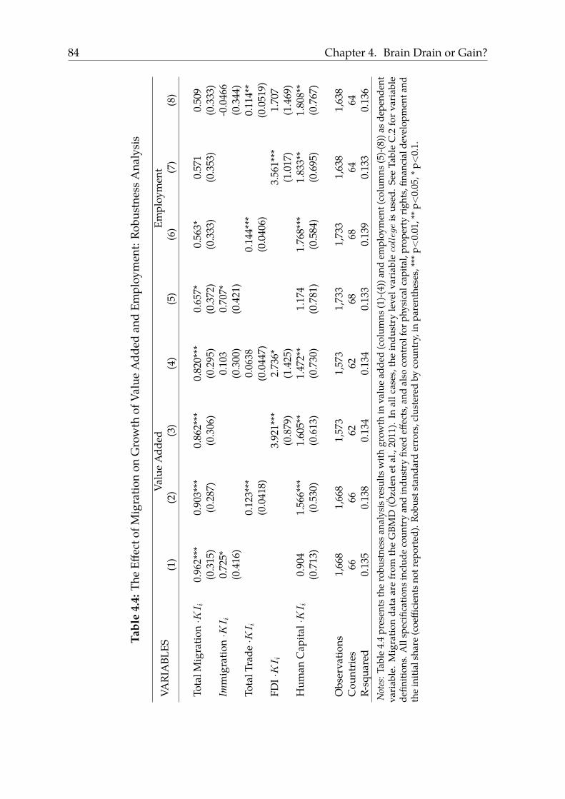
84 Chapter 4. Brain Drain or Gain?
Tabl
e4.
4:Th
eEff
ecto
fMig
ratio
non
Gro
wth
ofVa
lue
Add
edan
dEm
ploy
men
t:Ro
bust
ness
Ana
lysi
s
VARI
ABL
ESVa
lue
Add
edEm
ploy
men
t(1
)(2
)(3
)(4
)(5
)(6
)(7
)(8
)
Tota
lMig
ratio
n·KI i
0.96
2***
0.90
3***
0.86
2***
0.82
0***
0.65
7*0.
563*
0.57
10.
509
(0.3
15)
(0.2
87)
(0.3
06)
(0.2
95)
(0.3
72)
(0.3
33)
(0.3
53)
(0.3
33)
Imm
igra
tion·KI i
0.72
5*0.
103
0.70
7*-0
.046
6(0
.416
)(0
.300
)(0
.421
)(0
.344
)To
talT
rade
·KI i
0.12
3***
0.06
380.
144*
**0.
114*
*(0
.041
8)(0
.044
7)(0
.040
6)(0
.051
9)FD
I·KI i
3.92
1***
2.73
6*3.
561*
**1.
707
(0.8
79)
(1.4
25)
(1.0
17)
(1.4
69)
Hum
anC
apita
l·KI i
0.90
41.
566*
**1.
605*
*1.
472*
*1.
174
1.76
8***
1.83
3**
1.80
8**
(0.7
13)
(0.5
30)
(0.6
13)
(0.7
30)
(0.7
81)
(0.5
84)
(0.6
95)
(0.7
67)
Obs
erva
tions
1,66
81,
668
1,57
31,
573
1,73
31,
733
1,63
81,
638
Cou
ntri
es66
6662
6268
6864
64R-
squa
red
0.13
50.
138
0.13
40.
134
0.13
30.
139
0.13
30.
136
Not
es:T
able
4.4
pres
ents
the
robu
stne
ssan
alys
isre
sults
with
grow
thin
valu
ead
ded
(col
umns
(1)-(
4))a
ndem
ploy
men
t(co
lum
ns(5
)-(8)
)asd
epen
dent
vari
able
.Mig
ratio
nda
taar
efr
omth
eG
BMD
(Ozd
enet
al.,
2011
).In
allc
ases
,the
indu
stry
leve
lvar
iabl
ecollege
isus
ed.S
eeTa
ble
C.2
for
vari
able
defin
ition
s.A
llsp
ecifi
catio
nsin
clud
eco
untr
yan
din
dust
ryfix
edeff
ects
,and
also
cont
rolf
orph
ysic
alca
pita
l,pr
oper
tyrig
hts,
finan
cial
deve
lopm
enta
ndth
ein
itial
shar
e(c
oeffi
cien
tsno
trep
orte
d).R
obus
tsta
ndar
der
rors
,clu
ster
edby
coun
try,
inpa
rent
hese
s,**
*p<
0.01
,**p<
0.05
,*p<
0.1.

Chapter 4. Brain Drain or Gain? 85
This could explain an insignificant or negative effect of immigration on the growth ofknowledge-intensive industries.
Second, we include in the regressions an interaction term between the share of totaltrade (exports and imports of goods and services) to a country’s GDP (XMs) and theknowledge intensity of industries (KIi). Columns (2) and (6) of Table 4.4 present theresults for value added and employment respectively. Total trade has a positive andsignificant impact on the growth of knowledge-intensive industries, a finding that isin line with Romalis (2004), who demonstrates a similar effect of trade on internationalspecialization. Even so, our migration variable continues to enter the regressions witha positive and significant sign. A similar result was also reached when, instead oftotal trade, we interacted the share of exports (of goods and services) to a country’sGDP (Xs) and the knowledge intensity of industries (KIi). Columns (3) and (7) addFDI (FDIs) as an alternative openness variable and although its interaction withindustry knowledge intensity also influences specialization patterns, the migrationeffect remains very significant for growth in value added, but drops for growth inemployment (p=0.110).
Finally, columns (4) and (8) of Table 4.4 include immigration, trade and FDI simul-taneously. Not all openness variables are individually significant, likely due to theirhigh correlations, but the migration effect remains very significant for value addedgrowth. The significance of the effect on employment growth drops again, though(p=0.131).23 This could indicate that part of the specialization in skill-intensive manu-facturing industries is related to faster labor productivity growth. We also includedthe openness variables in the regressions from Table 4.2, and the finding that themigration effect is stronger in countries with initially low human capital levels is alsorobust to the inclusion of these additional variables.
Finally, we performed a number of additional robustness tests. We used the 1960migration to population ratio as an instrument for the 1980 ratio. This follows asimilar analysis in Ciccone and Papaioannou (2009) for human capital and aims toalleviate measurement error in 1980 migration levels.24 Data were again derivedfrom the GBMD (Ozden et al., 2011) and the WDI (2012). The first stage regressionrevealed that this is a relevant instrument to use. The F-values (between 21.55 and23.11) indicated that there is no weak identification problem. Table 4.5 presents theresults with value added (column (1)) and employment (column (2)), and the indus-
23This is not the case with the Brucker et al. (2013) data, where the β1-coefficient is positive andsignificant at the 10% for the case of employment.
24An alternative in the same spirit is to use the migration variable from the Brucker et al. (2013)database as an instrument for the variable from the GBMD (Ozden et al., 2011) database. The resultswere very similar to those shown in Table 4.5.

86 Chapter 4. Brain Drain or Gain?
Table 4.5: Instrumental Variable (IV) Regressions
VARIABLES Value Added Employment(1) (2)
Total Migration ·KIi 1.072*** 0.854**(0.370) (0.411)
Immigration ·KIi 0.0745 -0.0854(0.298) (0.342)
Total Trade ·KIi 0.0618 0.111**(0.0421) (0.0484)
FDI ·KIi 2.676* 1.634(1.383) (1.403)
Human Capital ·KIi 1.484** 1.828**(0.718) (0.764)
Observations 1,573 1,638Countries 62 64R-squared 0.134 0.135
First Stage F-value 21.55 23.11Notes: Table 4.5 presents the IV regressions results. Column (1) refers to the value added and column (2)to the employment regression. Migration data are from the GBMD (Ozden et al., 2011). In all cases, theindustry level variable college is used. See Table C.2 for variable definitions. All specifications includecountry and industry fixed effects, and also control for physical capital, property rights, financialdevelopment and the initial share (coefficients not reported). Robust standard errors, clustered bycountry, in parentheses, *** p<0.01, ** p<0.05, * p<0.1.
try level variable college. The conclusion that we reach also after the instrumentalvariable (IV) regression is that high-emigration countries experience higher growthin their knowledge-intensive industries. Note, furthermore, that by alleviating mea-surement error through the IV regressions, migration has again turned significant foremployment growth.
As an additional robustness test, we also excluded every country and industryone-by-one. This had no effect on the overall results though for a few combinations ofomitted countries, industries and knowledge intensity measures, significance woulddrop.25 The specification where we allow for a differential effect in low human capitalcountries remained unaffected to the exclusion of each and every country or industry.
25Value added regressions using the college variable remained robust throughout.

Chapter 4. Brain Drain or Gain? 87
4.6 Discussion
Analyzing the effects of migration on industrial specialization, we conclude thatindustries that rely heavily on human capital grow faster in high-emigration countriesand that this relationship is driven by high- and medium-skilled migrants. Our studydiffers from the existing empirical ‘brain drain/gain’ literature (e.g. Beine et al., 2001,2008; Docquier et al., 2008; Beine et al., 2010, 2011; Di Maria & Lazarova, 2012) inthat we infer an effect on country human capital from observing specialization inknowledge-intensive industries rather than directly testing for the effect of migrationon human capital formation. Our conclusions are also different, in part. In contrast tomost studies we find that, although stronger among low-human-capital countries, a‘brain gain’ effect dominates all countries. We argue that there are two complementaryexplanations for this: the broader view on human capital we adopt and the self-reinforcing effects of SBTC.
Overall, the recent empirical macro-literature provides some evidence for the‘brain gain’. However, the number of origin countries that gain (or lose) from emi-gration and the magnitude of these gains (or losses) vary. Examining 37 developingcountries, Beine et al. (2001) find a positive and significant impact of gross emigrationon human capital, particularly for low-GDP countries. In a larger sample of countries(127) and using tertiary (rather than total) emigration, Beine et al. (2008) also findevidence for a ‘brain gain’. It is the countries with low levels of human capital andlow emigration rates that gain the most from high-skilled emigration (e.g. China,India, Indonesia, Brazil, Egypt, Bangladesh) but, since the absolute gains outweigh theabsolute losses, the developing world benefits as a whole. On the contrary, Docquier etal. (2008) reach more pessimistic conclusions, as they find that high-skilled emigrationnegatively impacts the post-secondary-educated population in the developing world.Studying the effect of migration on the level and the composition of human capital,Di Maria and Lazarova (2012) also conclude that emigration has potentially detri-mental impacts on economic growth, depending on a country’s level of technologicalsophistication. Finally, in a panel set-up, Beine et al. (2011) provide evidence for a‘brain gain’, particularly for low-income countries.
We find that the positive effects of emigration on industrial specialization accrueto all countries. One explanation relates to the definition of human capital we adopt.To begin with, we do not equate ‘brain drain’ with high-skilled emigration. We ratherfocus on all migrants and show that it is not only the high- but also the medium-skilledones that trigger the growth in knowledge-intensive industries. This distinguishesour paper from the recent literature (e.g. Beine et al., 2011) and is more in line with

88 Chapter 4. Brain Drain or Gain?
the argument of Beine et al. (2001) that ‘brain drain’ implies migrants with above-average skills rather than “engineers, physicians, scientists or other very highly skilledprofessional” (p. 276).
By the same token, specialization in human-capital-intensive industries relatesto increases in the broader human capital rather than only in the tertiary-educatedpopulation. If, for example, a population changes from one where primary educationis most prevalent to one where secondary education is dominant, this qualifies, by allaccounts, as an increase in the stock of human capital of the economy. Those secondary-schooled workers may not be “sufficiently skilled” for a knowledge-intensive industryin a country close to the technological frontier, but they may well be qualified inless-advanced economies. As a result of this increase in human capital endowments,relatively knowledge-intensive industries will grow faster. Focusing solely on tertiaryeducation, by looking at high-skilled emigration and how it affects high-skilled humancapital at home, leaves out any changes occurring at lower levels, underestimatingthe full extent of skill upgrading that is taking place.
The typical model in the ‘brain drain/gain’ literature uses a fairly stylized produc-tion sector, which is then used to inform the likely effects of migration. Furthermore,the typical direct empirical test of the link between greater emigration and increasesin schooling is unlikely to capture any indirect effects. The work of Acemoglu (1998,1999, 2002) suggests that modeling a skill-intensive and a labor-intensive sector willoften lead to SBTC. Under SBTC, any increases in human capital will lead to greaterdemand for skilled workers and provide the incentives for further increases in thesupply of human capital. A single-sector model will not give rise to such dynamics.Furthermore, a direct test of the effect of emigration on human capital may relate tothe first round of human capital increases, but if there is SBTC, there is a plausibleargument that the further endogenous increases in demand for and supply of humancapital can also be related to greater initial emigration. Our approach attributes thefull effect to emigration since we look at the end result of human capital increases andsectoral specialization after, a maximum of, two decades.
4.7 Concluding Remarks
International migration is a major aspect of globalization, central in both academicand policy-related debates. In this paper, we have studied the impact of emigrationon the human capital of sending countries by analyzing industry growth patternsand have relied on a dataset that covers up to 68 countries and 28 manufacturing

Chapter 4. Brain Drain or Gain? 89
industries over the period 1980-2000.Our results show a ‘brain gain’, whereby high-emigration countries see faster
growth in knowledge-intensive manufacturing industries. This specialization effectis only to be expected if the net effect of migration on human capital is positive. Thesize of this effect is considerable, at about one- to two-thirds as large as the effectof initial human capital levels on specialization, the education channel of Cicconeand Papaioannou (2009). Both high- and medium-skilled migration drive the growthof knowledge-intensive industries. Furthermore, countries with initially low levelsof human capital benefit substantially more. Our results are not driven by generaleconomic openness, as controlling for immigration, trade and FDI does not alter ourconclusions. The source of migration data that is used does not drive our results either.Compared with the existing literature, we find that a broader group of countriesbenefits, in part (we argue) because we do not solely focus on tertiary-educatedmigrants and human capital and because our approach would also capture the effectsof SBTC.
Important to note is also how the changes in the production structure that wefind relate to economic growth. Hausmann, Hwang, and Rodrik (2007) have shownthat the type of goods a country specializes in matters for its economic performance.Specialization in goods that rich countries export induces faster growth than special-ization in other goods. From their analysis, we can thus infer a connection between theproduction of more sophisticated goods and economic growth. Our analysis also re-lates to these broader consequences for the economy, as it shows how migration affectsthe production structure and shifts specialization towards sophisticated industries,which in turn can have favorable implications for economic development.
The limitations of our study also need to be addressed. To begin with, we analyzeindustry growth patterns rather than directly linking (high-skilled) migration toincreases in the number of high-skilled people. The benefits of this strategy havealready been outlined, but there is also a limitation to it. The lack of specificity on theprecise links along the causal chain from emigration to specialization also means thatit may be some other variable that is driving or moderating the effect. Furthermore,high-skilled emigration impacts areas which our study does not cover. Bhargava etal. (2011), for example, examine how human development indicators (e.g. healthoutcomes) are affected by physician emigration in developing countries and do notfind compelling evidence for a ‘brain gain’.
Important to clarify at this point is that our study finds an average positive effect ofemigration on industry growth, for the countries that form our sample. This is not to say,however, that an indefinite outflow of high-skilled people won’t entail detrimental
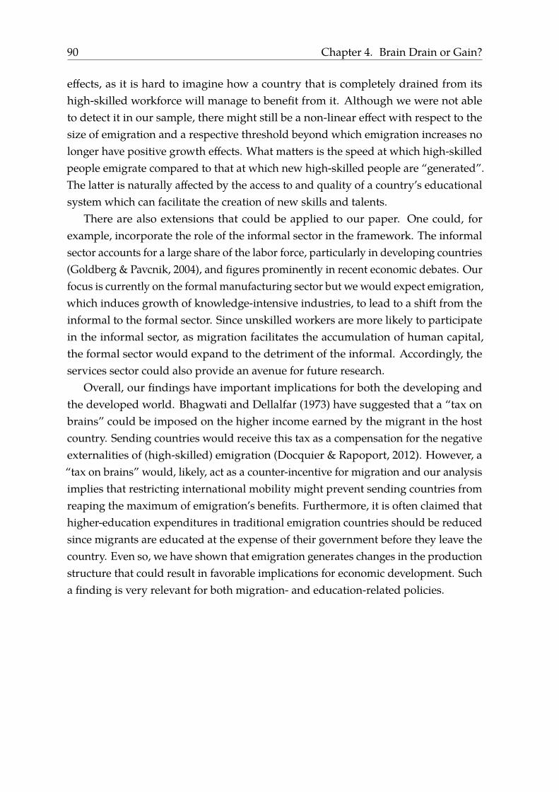
90 Chapter 4. Brain Drain or Gain?
effects, as it is hard to imagine how a country that is completely drained from itshigh-skilled workforce will manage to benefit from it. Although we were not ableto detect it in our sample, there might still be a non-linear effect with respect to thesize of emigration and a respective threshold beyond which emigration increases nolonger have positive growth effects. What matters is the speed at which high-skilledpeople emigrate compared to that at which new high-skilled people are “generated”.The latter is naturally affected by the access to and quality of a country’s educationalsystem which can facilitate the creation of new skills and talents.
There are also extensions that could be applied to our paper. One could, forexample, incorporate the role of the informal sector in the framework. The informalsector accounts for a large share of the labor force, particularly in developing countries(Goldberg & Pavcnik, 2004), and figures prominently in recent economic debates. Ourfocus is currently on the formal manufacturing sector but we would expect emigration,which induces growth of knowledge-intensive industries, to lead to a shift from theinformal to the formal sector. Since unskilled workers are more likely to participatein the informal sector, as migration facilitates the accumulation of human capital,the formal sector would expand to the detriment of the informal. Accordingly, theservices sector could also provide an avenue for future research.
Overall, our findings have important implications for both the developing andthe developed world. Bhagwati and Dellalfar (1973) have suggested that a “tax onbrains” could be imposed on the higher income earned by the migrant in the hostcountry. Sending countries would receive this tax as a compensation for the negativeexternalities of (high-skilled) emigration (Docquier & Rapoport, 2012). However, a“tax on brains” would, likely, act as a counter-incentive for migration and our analysisimplies that restricting international mobility might prevent sending countries fromreaping the maximum of emigration’s benefits. Furthermore, it is often claimed thathigher-education expenditures in traditional emigration countries should be reducedsince migrants are educated at the expense of their government before they leave thecountry. Even so, we have shown that emigration generates changes in the productionstructure that could result in favorable implications for economic development. Sucha finding is very relevant for both migration- and education-related policies.

APPENDIX C
Appendix Chapter 4
Table C.1: List of Countries Included in the Analysis and Key Figures
Country Mig
ratio
n:to
tal
GBM
D
Mig
ratio
n:to
tal
Bruc
kere
tal.
(201
3)
Mig
ratio
n:hi
gh-
and
med
ium
-ski
lled
Bruc
kere
tal.
(201
3)
Mig
ratio
n:lo
w-s
kille
dBr
ucke
reta
l.(2
013)
Popu
latio
n:to
tal
WD
I(20
12)
Argentina 315269 104681 62213 42468 28131040Australia 222632 116553 65888 50665 14692000Austria 618810 475561 303756 171805 7549433Bangladesh 5047223 33023 18820 14203 80624423Barbados 68467 53860 31955 21905 248796Belgium 414680 212693 87101 125592 9859242Bolivia 166734 15689 10250 5439 5352649Botswana 79600 557 148 409 996211Brazil 302935 60836 32373 28463 121711864Cameroon 138279 8683 4558 4125 9109727Canada 1211849 765558 475352 290206 24593000Central African Republic 37732 1000 600 400 2273630Chile 401856 69173 47292 21881 11178817China 4174988 353506 190792 162714 981235000Colombia 719142 105073 64755 40318 26874906Costa Rica 51792 20198 12262 7936 2343345Cyprus 154456 95406 58402 37004 685510Denmark 249239 146827 80552 66275 5123027
91

92 Appendix C. Chapter 4
Ecuador 148834 63212 34951 28261 7957811Egypt 1030182 135219 94170 41049 44952497El Salvador 159304 58670 24136 34534 4656263Finland 344332 272761 118829 153932 4779535France 1423049 394504 246033 148471 55166046Ghana 380565 35998 21794 14204 10922708Greece 1183275 696743 208807 487936 9642505Guatemala 97580 39994 17038 22956 7036484Honduras 81455 24671 12772 11899 3627640Iceland 19147 9275 5043 4232 228138India 7582096 647840 401425 246415 700058589Indonesia 489804 137875 59543 78332 150820044Iran 529305 138787 103530 35257 38576541Ireland 911750 865101 440364 424737 3412800Israel 379720 69949 49611 20338 3878000Italy 4510364 2870494 645551 2224943 56433883Jamaica 426824 319424 183263 136161 2133000Japan 602467 210892 159699 51193 116782000Jordan 628401 28722 18612 10110 2181000Kenya 318867 67241 38585 28656 16267558Malawi 263950 4114 1806 2308 6239898Malaysia 409630 53213 38310 14903 13832586Mauritius 66983 37380 17955 19425 966000Mexico 2579330 1302092 282826 1019266 68776411Netherlands 726627 510463 313483 196980 14149800New Zealand 236982 129900 90572 39328 3113000Norway 167770 128230 56513 71717 4085620Pakistan 3970210 196355 82955 113400 80492664Panama 108197 42371 31332 11039 1953029Peru 134083 51247 37745 13502 17286832Philippines 980831 438896 327956 110940 47063923Portugal 1872021 878851 93776 785075 9766312Republic of Korea 1089819 196121 149829 46292 38124000Senegal 213314 23123 3085 20038 5414070Singapore 150803 24465 15349 9116 2414000South Africa 249121 87010 56809 30201 27576000Spain 1900957 831694 142968 688726 37439035
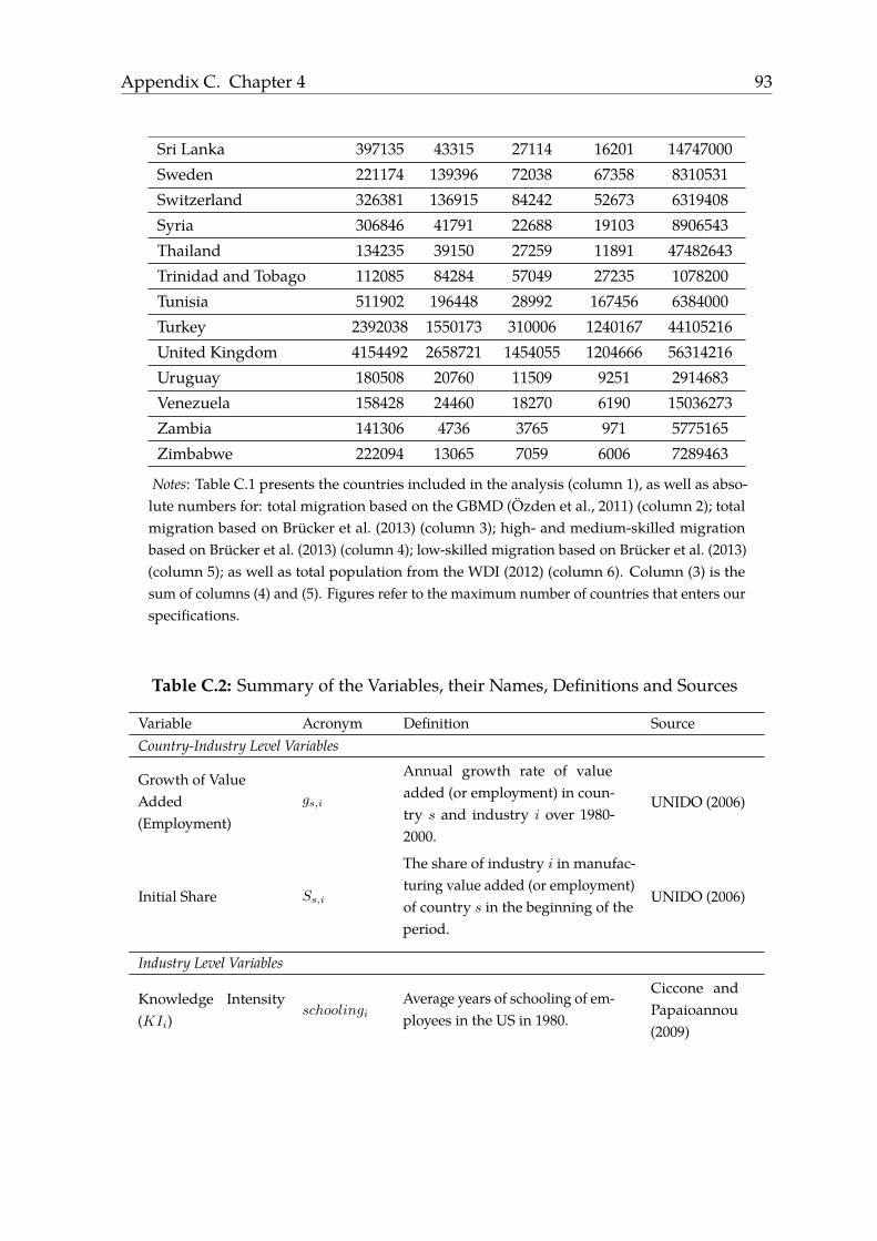
Appendix C. Chapter 4 93
Sri Lanka 397135 43315 27114 16201 14747000Sweden 221174 139396 72038 67358 8310531Switzerland 326381 136915 84242 52673 6319408Syria 306846 41791 22688 19103 8906543Thailand 134235 39150 27259 11891 47482643Trinidad and Tobago 112085 84284 57049 27235 1078200Tunisia 511902 196448 28992 167456 6384000Turkey 2392038 1550173 310006 1240167 44105216United Kingdom 4154492 2658721 1454055 1204666 56314216Uruguay 180508 20760 11509 9251 2914683Venezuela 158428 24460 18270 6190 15036273Zambia 141306 4736 3765 971 5775165Zimbabwe 222094 13065 7059 6006 7289463
Notes: Table C.1 presents the countries included in the analysis (column 1), as well as abso-lute numbers for: total migration based on the GBMD (Ozden et al., 2011) (column 2); totalmigration based on Brucker et al. (2013) (column 3); high- and medium-skilled migrationbased on Brucker et al. (2013) (column 4); low-skilled migration based on Brucker et al. (2013)(column 5); as well as total population from the WDI (2012) (column 6). Column (3) is thesum of columns (4) and (5). Figures refer to the maximum number of countries that enters ourspecifications.
Table C.2: Summary of the Variables, their Names, Definitions and Sources
Variable Acronym Definition SourceCountry-Industry Level Variables
Growth of ValueAdded(Employment)
gs,i
Annual growth rate of valueadded (or employment) in coun-try s and industry i over 1980-2000.
UNIDO (2006)
Initial Share Ss,i
The share of industry i in manufac-turing value added (or employment)of country s in the beginning of theperiod.
UNIDO (2006)
Industry Level Variables
Knowledge Intensity(KIi)
schoolingiAverage years of schooling of em-ployees in the US in 1980.
Ciccone andPapaioannou(2009)
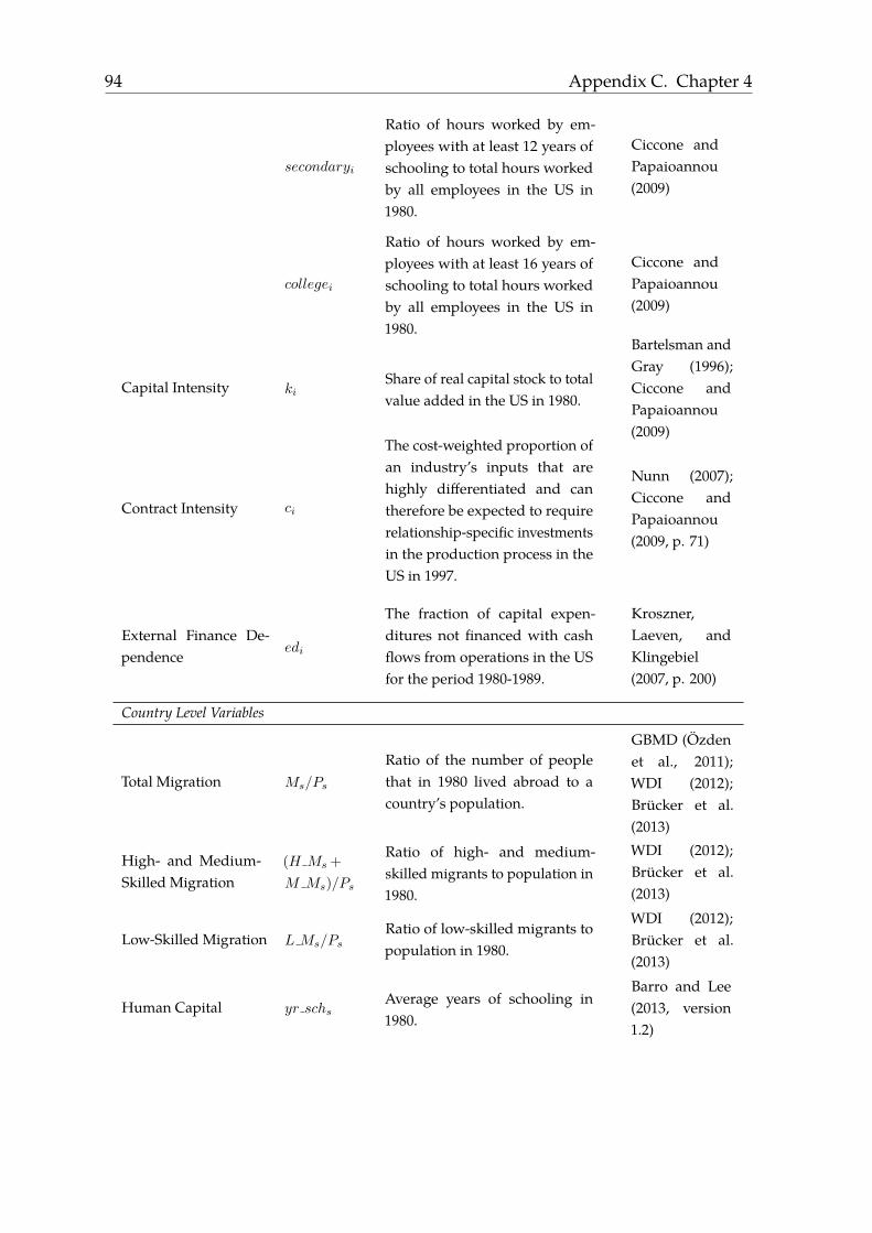
94 Appendix C. Chapter 4
secondaryi
Ratio of hours worked by em-ployees with at least 12 years ofschooling to total hours workedby all employees in the US in1980.
Ciccone andPapaioannou(2009)
collegei
Ratio of hours worked by em-ployees with at least 16 years ofschooling to total hours workedby all employees in the US in1980.
Ciccone andPapaioannou(2009)
Capital Intensity kiShare of real capital stock to totalvalue added in the US in 1980.
Bartelsman andGray (1996);Ciccone andPapaioannou(2009)
Contract Intensity ci
The cost-weighted proportion ofan industry’s inputs that arehighly differentiated and cantherefore be expected to requirerelationship-specific investmentsin the production process in theUS in 1997.
Nunn (2007);Ciccone andPapaioannou(2009, p. 71)
External Finance De-pendence
edi
The fraction of capital expen-ditures not financed with cashflows from operations in the USfor the period 1980-1989.
Kroszner,Laeven, andKlingebiel(2007, p. 200)
Country Level Variables
Total Migration Ms/Ps
Ratio of the number of peoplethat in 1980 lived abroad to acountry’s population.
GBMD (Ozdenet al., 2011);WDI (2012);Brucker et al.(2013)
High- and Medium-Skilled Migration
(H Ms +
M Ms)/Ps
Ratio of high- and medium-skilled migrants to population in1980.
WDI (2012);Brucker et al.(2013)
Low-Skilled Migration L Ms/Ps
Ratio of low-skilled migrants topopulation in 1980.
WDI (2012);Brucker et al.(2013)
Human Capital yr schsAverage years of schooling in1980.
Barro and Lee(2013, version1.2)

Appendix C. Chapter 4 95
lscs
Percentage of complete sec-ondary schooling attained in acountry’s population in 1980.
Barro and Lee(2013, version1.2)
lhcs
Percentage of complete tertiaryschooling attained in a country’spopulation in 1980.
Barro and Lee(2013, version1.2)
Physical Capital Ks/Ys Capital-output ratio in 1980.Klenow andRodrıguez-Clare (2005)
Property Rights Ps
Index for the legal system and se-curity of property rights in 1985.
Gwartney et al.(2012)
Financial Development FDs
The domestic credit to privatesector relative to GDP in the year1980.
WDI (2012)
Immigration IMs/Ps
Share of immigrants (the stock offoreign-born people) in a coun-try’s population in 1980.
GBMD (Ozdenet al., 2011);WDI (2012)
Exports XsExports of goods and services asa share to GDP in 1980.
Heston, Sum-mers, and Aten(2012); UnitedNations Statis-tics Division(2012)
Total Trade XMs
Exports and imports of goodsand services as a share to GDPin 1980.
Heston et al.(2012); UnitedNations Statis-tics Division(2012)
Foreign Direct Invest-ment
FDIsNet inflows of FDI to GDP in1980.
WDI (2012)
Human CapitalDummy Hs
Dummy variable equal to one forcountries in the bottom quartileof the world human-capital distri-bution (lhcs < 0.0074), zero oth-erwise. The quartile is identifiedbased on all countries includedin Barro and Lee (2013, version1.2) and refers to the year 1980.
Barro and Lee(2013, version1.2)


CHAPTER 5
Samenvatting (Dutch Summary)
Er is veel consensus in de literatuur met betrekking tot het belang van onderwijs, datwil zeggen menselijk kapitaal. Zowel voor de economie als voor de maatschappij
als geheel heeft onderwijs grote waarde: het genereert geldelijke omzet, maar ooksociaal rendement, zoals effecten op misdaadcijfers, volksgezondheid, sterftecijfers,vruchtbaarheid, politieke participatie (bv. Moretti, 2005; Lochner, 2011). Daaromspeelt onderwijs zo’n centrale rol in het economische en politieke debat.
Dit proefschrift onderzoekt het belang van onderwijs, en dus menselijk kapitaal,voor het faciliteren van snellere economische groei. Het heeft een plaats binnen eenbrede, recente opleving van literatuur waarin gezocht wordt naar een beter begripvan menselijk kapitaal en de effecten ervan op groei (bv. Fraumeni, 2015; Lucas,2015). Er bestaan verschillende theorieen met betrekking tot de manieren waaropmenselijk kapitaal economische groei beınvloedt (bv. Nelson & Phelps, 1966; Mankiwet al., 1992). In empirisch onderzoek wordt gewoonlijk naar deze relatie gekeken doormiddel van omvangrijke datasets, empirische opstellingen en methodologieen.
Elk hoofdstuk van dit proefschrift beantwoordt een specifieke vraag met betrekkingtot de effecten van menselijk kapitaal op economische groei.
Een standaard uitgangspunt bij groei- of ontwikkelingsrekening is de aanname vanconstante arbeidsdiensten per gewerkt uur. Deze aanname kan echter ongeldig blijkenwegens vintage effecten: pas afgestudeerden wijken van eerdere cohorten af metbetrekking tot de arbeidsdiensten per gewerkt uur die zij leveren. Dit kan bijvoorbeeldhet gevolg zijn van betere scholing of ‘on-the-job training’. Bowlus en Robinson (2012)hebben aangetoond dat vintage effecten in de Verenigde Staten aanzienlijk zijn (zo zijnbijvoorbeeld de arbeidsdiensten per gewerkt uur van hooggeschoolde werknemers inde loop van de tijd toegenomen). Daardoor wordt de groei van menselijk kapitaalonderschat en die van de totale factor productiviteit (TFP) overschat.
In Hoofdstuk 2 volg ik de aanpak van Bowlus en Robinson (2012) en gebruik
97
98 Chapter 5. Samenvatting
ik een nieuwe maatstaf voor menselijk kapitaal waarin rekening wordt gehoudenmet vintage effecten. Op deze manier laat ik de veronderstelling los dat een jaar opschool een constante hoeveelheid menselijk kapitaal oplevert. De introductie vandeze vintage effecten bij het berekenen van de groei verhoogt de arbeidsdienstenvan hooggeschoolde werknemers in de Verenigde Staten en het Verenigd Koninkrijkvergeleken met de standaard groeirekening. Daarentegen is de bijdrage van menselijkkapitaal aan groei in continentale Europese landen (Frankrijk, Duitsland, Italie, Ned-erland en Spanje) tussen 1995 en 2005 gedaald. In die periode speelden vintageeffecten van menselijk kapitaal een grote rol in de verklaring van het verschil in detrans-Atlantische productiviteitsgroei.
Het beschrijven van groei en ontwikkeling mag een belangrijk diagnostisch middelzijn, het negeert alle indirecte bijdragen van menselijk kapitaal. Deze methodiekenhouden geen rekening met interacties tussen efficientie en fysieke als ook menselijkekapitaalopbouw (Caselli, 2005; Barro & Lee, 2015). Als gevolg hiervan wordt de rolvan menselijk kapitaal niet volledig meegewogen. Deze indirecte kanalen implicerendat er externaliteiten bestaan.
Externaliteiten van menselijk kapitaal komen tot uiting als de maatschappelijkerendementen van onderwijs hoger zijn dan de persoonlijke rendementen (bv. Krueger& Lindahl, 2001). Dit betekent dat de voordelen van menselijk kapitaal niet beperktblijven tot de persoon die onderwijs krijgt, maar dat ze ook merkbaar zijn voor medew-erkers, de gemeenschap, het land en zelfs andere landen. Als alleen het persoonlijkerendement van onderwijs wordt meegenomen, zou dat dus tot een onderwaarderingvan het belang van menselijk kapitaal leiden. Dat kan weer een verkeerde invloedhebben op overheidsbeleid ten aanzien van onderwijsvoorzieningen.
Het bestaan van externaliteiten komt op twee manieren in de literatuur tot uit-drukking: de eerste heeft te maken met de “spill-over” van menselijk kapitaal diede productiviteit van anderen kan verhogen (bv. Lucas, 1988) en de tweede koppeltmenselijk kapitaal aan technologische vooruitgang en adoptie van nieuwe technolo-gie (bv. Nelson & Phelps, 1966; Romer, 1990). Onderwijs maakt werknemers meerinnovatief en daardoor bepaalt het menselijk kapitaal het niveau van technologischevooruitgang. Bovendien zijn minder geavanceerde economieen afhankelijk van deadoptie (imitatie) van nieuwe en meer productieve technologieen om bij te blijven.Menselijk kapitaal is dus instrumenteel in dit proces (Nelson & Phelps, 1966; Benhabib& Spiegel, 1994, 2005).
In Hoofdstuk 3 kijk ik opnieuw naar het vermogen van menselijk kapitaal omexternaliteiten te genereren door middel van technologische vooruitgang en adoptievan technologie. Ik wijk van de veronderstelling af, dat de bijdrage van menselijk

Chapter 5. Samenvatting 99
kapitaal kan worden gemeten aan de persoonlijke opbrengst die tot uitdrukkingkomt in het loonstrookje. Om potentiele externaliteiten op te sporen, gebruik ik eeneconometrische methode die menselijk kapitaal met de totale factor productiviteit(TFP) verbindt. Empirisch onderzoek over dit onderwerp heeft gemengde resultatenopgeleverd (bv. Vandenbussche et al., 2006; Inklaar et al., 2008). De bijdrage vanhoofdstuk 3 ligt in het gebruik van state-of-the-art TFP-data, waar het prive-rendementvan scholing uit is gehaald. Dat maakt het mogelijk om conclusies te trekken over hetbestaan van externaliteiten.
Uit mijn analyse komt een ruimer bestaan van externaliteiten naar voren dan uitde literatuur tot nu toe. Externaliteiten worden gegenereerd door tertiair opgeleidemensen en hangen in hoge mate af van het niveau van de technologische ontwikkelingvan een land. Ik vind ook bewijs dat niet alle soorten/niveaus van onderwijs (tertiair,secundair, primair) dezelfde invloed hebben op de TFP-groei. De samenstelling vanmenselijk kapitaal is belangrijk.
Handel, FDI en migratie vormen de globaliseringskrachten/-kanalen waardoortechnologie wordt verspreid over verschillende landen. Menselijk kapitaal faciliteertdeze verspreiding door zijn effect op de absorptiecapaciteit van de economie (bv.Keller, 2004). In het geval van migratie ligt het ingewikkeld: als mensen landsgrenzenoversteken, wordt het niveau van menselijk kapitaal van zowel het thuis- als hetgastland beınvloed. De richting waarin het menselijk kapitaal van het thuisland wordtbeınvloed, is a priori onbekend. Er zijn zowel negatieve als positieve krachten: aande ene kant wordt het menselijk kapitaal negatief beınvloed als hooggeschooldenmigreren (‘brain drain’). Aan de andere kant is er steeds meer bewijs dat emigratie devorming van menselijk kapitaal in het thuisland bevordert via feedback mechanismenzoals terugkerende migranten, overgemaakt geld, netwerken en stimulerende effecten(‘brain gain’). Gezien de centrale rol van menselijk kapitaal voor economische groei,is het van groot belang om uit te zoeken hoe migratie de richting daarvan beınvloedt.
Uiteindelijk ligt er dus een empirische vraag: wat is het effect van emigratie ophet menselijk kapitaal van het thuisland? Emigratie kan de prikkels verbeteren omvaardigheden te verwerven of te verbeteren: als de mogelijkheid om te migreren deverwachte opbrengsten aan onderwijs verbetert, worden de prikkels om een opleid-ing te krijgen sterker en dat leidt tot een toename van het menselijk kapitaal in hetthuisland. Mountford (1997) en Stark et al. (1997, 1998) hebben als eersten het ideeontwikkeld dat “verwachtingen over toekomstige migratiekansen invloed hebben oponderwijsbeslissingen” (Docquier & Rapoport, 2012, p. 701).
In Hoofdstuk 4 onderzoek ik potentiele internationale “spill-overs” van menselijkkapitaal. Ik analyseer de impact van migratie op het menselijk kapitaal van het thuis-

100 Chapter 5. Samenvatting
land en kom tot de conclusie dat landen met een hogere emigratie van vakbekwamewerknemers een snellere groei in hun kennisintensieve industrieen laten zien. Mijnbevindingen over de totale migratie laten zich met name herleiden tot de migratie vanzowel hoog- als middelhoogopgeleide werknemers, maar tonen geen positief effectvan de migratie van laaggeschoolden. Dit suggereert, wellicht verrassend, een ‘braingain’ in plaats van ‘brain drain’.
Samenvattend kunnen we zeggen dat we veel weten over de mogelijke voordelen-monetair en niet-monetair- van onderwijs op zowel individueel als nationaal en zelfsinternationaal niveau. Verder onderzoek kan individuen en de samenleving als geheelhelpen om de voordelen en de kosten beter tegen elkaar af te wegen en beleidsmakerseen richtlijn in handen te geven.

References
Abramovitz, M. (1956). Resource and Output Trends in the United States Since 1870.National Bureau of Economic Research, Inc., 1-23.
Acemoglu, D. (1998). Why Do New Technologies Complement Skills? DirectedTechnical Change and Wage Inequality. The Quarterly Journal of Economics, 113(4),1055-1089.
Acemoglu, D. (1999). Changes in Unemployment and Wage Inequality: An AlternativeTheory and Some Evidence. American Economic Review, 89(5), 1259-1278.
Acemoglu, D. (2002). Technical Change, Inequality, and the Labor Market. Journal ofEconomic Literature, 40(1), 7-72.
Acemoglu, D., & Angrist, J. (2001). How Large are Human-Capital Externalities?Evidence from Compulsory-Schooling Laws. In NBER Macroeconomics Annual2000, Volume 15 (p. 9-74). National Bureau of Economic Research, Inc.
Acemoglu, D., Johnson, S., Robinson, J. A., & Yared, P. (2005). From Education toDemocracy? American Economic Review, 95(2), 44-49.
Adams, R. H., & Cuecuecha, A. (2013). The Impact of Remittances on Investment andPoverty in Ghana. World Development, 50(C), 24-40.
Aghion, P., & Howitt, P. (2009). The Economics of Growth (MIT Press, Ed.).Anderson, D. M. (2014). In School and Out of Trouble? The Minimum Dropout Age
and Juvenile Crime. The Review of Economics and Statistics, 96(2), 318-331.Ang, J. B., Madsen, J. B., & Islam, R. M. (2011). The Effects of Human Capital
Composition on Technological Convergence. Journal of Macroeconomics, 33(3),465-476.
Barro, R. J. (1996). Determinants of Economic Growth: A Cross-Country Empirical Study(NBER Working Papers No. 5698). National Bureau of Economic Research, Inc.
Barro, R. J., & Lee, J.-W. (1994). Sources of Economic Growth. Carnegie-RochesterConference Series on Public Policy, 40(1), 1-46.
Barro, R. J., & Lee, J.-W. (2013). A New Data Set of Educational Attainment in theWorld, 1950–2010. Journal of Development Economics, 104(C), 184-198.
101

102 References
Barro, R. J., & Lee, J.-W. (2015). Education Matters: Global Schooling Gains From the 19thto the 21st Century (Oxford University Press USA, Ed.).
Bartelsman, E. J., & Gray, W. (1996). The NBER Manufacturing Productivity Database(Working Paper No. 205). National Bureau of Economic Research, Inc.
Batista, C., Lacuesta, A., & Vicente, P. C. (2012). Testing the ‘Brain Gain’ Hypothesis:Micro Evidence from Cape Verde. Journal of Development Economics, 97(1), 32-45.
Becker, G. S. (2007). Health as Human Capital: Synthesis and Extensions. OxfordEconomic Papers, 59(3), 379-410.
Beine, M., Docquier, F., & Oden-Defoort, C. (2011). A Panel Data Analysis of the BrainGain. World Development, 39(4), 523-532.
Beine, M., Docquier, F., & Rapoport, H. (2001). Brain Drain and Economic Growth:Theory and Evidence. Journal of Development Economics, 64(1), 275-289.
Beine, M., Docquier, F., & Rapoport, H. (2008). Brain Drain and Human CapitalFormation in Developing Countries: Winners and Losers. Economic Journal,118(528), 631-652.
Beine, M., Docquier, F., & Rapoport, H. (2010). On the Robustness of Brain GainEstimates. Annals of Economics and Statistics(97-98), 143-165.
Benhabib, J., Perla, J., & Tonetti, C. (2014). Catch-up and Fall-back through Innovationand Imitation. Journal of Economic Growth, 19(1), 1-35.
Benhabib, J., & Spiegel, M. M. (1994). The Role of Human Capital in EconomicDevelopment Evidence from Aggregate Cross-Country Data. Journal of MonetaryEconomics, 34(2), 143-173.
Benhabib, J., & Spiegel, M. M. (2005). Human Capital and Technology Diffusion. InP. Aghion & S. N. Durlauf (Eds.), (Vol. 1, p. 935-966). Elsevier.
Benos, N., & Zotou, S. (2014). Education and Economic Growth: A Meta-RegressionAnalysis. World Development, 64(C), 669-689.
Ben-Porath, Y. (1967). The Production of Human Capital and the Life Cycle of Earnings.Journal of Political Economy, 75(4), 352-365.
Bhagwati, J., & Dellalfar, W. (1973). The Brain Drain and Income Taxation. WorldDevelopment, 1(1-2), 94-101.
Bhagwati, J., & Hamada, K. (1974). The Brain Drain, International Integration ofMarkets for Professionals and Unemployment: A Theoretical Analysis. Journalof Development Economics, 1(1), 19-42.
Bhargava, A., Docquier, F., & Moullan, Y. (2011). Modeling the Effects of PhysicianEmigration on Human Development. Economics & Human Biology, 9(2), 172-183.
Bils, M., & Klenow, P. J. (2000). Does Schooling Cause Growth? American EconomicReview, 90(5), 1160-1183.
References 103
Borjas, G. J. (1989). Immigrant and Emigrant Earnings: A Longitudinal Study.Economic Inquiry, 27(1), 21-37.
Bowlus, A. J., & Robinson, C. (2012). Human Capital Prices, Productivity, and Growth.American Economic Review, 102(7), 3483-3515.
Brucker, H., Capuano, S., & Marfouk, A. (2013). Education, Gender and InternationalMigration: Insights from a Panel-Dataset 1980-2010, mimeo. Retrieved fromhttp://www.iab.de/en/daten/iab-brain-drain-data.aspx
Byrne, D. M., Fernald, J. G., & Reinsdorf, M. B. (2016). Does the United States Havea Productivity Slowdown or a Measurement Problem? Brookings Papers onEconomic Activity, 47(Spring), 109-182.
Caselli, F. (2005). Accounting for Cross-Country Income Differences. In P. Aghion &S. Durlauf (Eds.), Handbook of Economic Growth (Vol. 1, p. 679-741). Elsevier.
Cerina, F., & Manca, F. (2016). Catch me if you Learn: Development-Specific Educationand Economic Growth. Macroeconomic Dynamics, 1–43.
Cette, G., Fernald, J., & Mojon, B. (2016). The Pre-Great Recession Slowdown inProductivity. European Economic Review, 88(C), 3-20.
Chen, H.-J. (2009). A Brain Gain Or A Brain Drain? Migration, Endogenous Fertility,And Human Capital Formation. Economic Inquiry, 47(4), 766-782.
Chor, D. (2010). Unpacking Sources of Comparative Advantage: A QuantitativeApproach. Journal of International Economics, 82(2), 152-167.
Ciccone, A., & Papaioannou, E. (2009). Human Capital, the Structure of Production,and Growth. The Review of Economics and Statistics, 91(1), 66-82.
Cohen, D., & Leker, L. (2014). Health and Education: Another Look with the Proper Data(CEPR Discussion Papers No. 9940). C.E.P.R. Discussion Papers.
Cohen, D., & Soto, M. (2007). Growth and Human Capital: Good data, Good Results.Journal of Economic Growth, 12(1), 51-76.
Costinot, A. (2009). On the Origins of Comparative Advantage. Journal of InternationalEconomics, 77(2), 255-264.
Currie, J., & Moretti, E. (2003). Mother’s Education and the Intergenerational Trans-mission of Human Capital: Evidence from College Openings. The QuarterlyJournal of Economics, 118(4), 1495-1532.
de la Fuente, A., & Domenech, R. (2015). Educational Attainment in the OECD,1960–2010. Updated Series and a Comparison with Other Sources. Economics ofEducation Review, 48(C), 56-74.
Delgado, M. S., Henderson, D. J., & Parmeter, C. F. (2014). Does Education Matter forEconomic Growth? Oxford Bulletin of Economics and Statistics, 76(3), 334-359.
104 References
Di Maria, C., & Lazarova, E. A. (2012). Migration, Human Capital Formation, andGrowth: An Empirical Investigation. World Development, 40(5), 938-955.
Docquier, F., Faye, O., & Pestieau, P. (2008). Is Migration a Good Substitute forEducation Subsidies? Journal of Development Economics, 86(2), 263-276.
Docquier, F., & Rapoport, H. (2012). Globalization, Brain Drain, and Development.Journal of Economic Literature, 50(3), 681-730.
Dumont, J.-C., Spielvogel, G., & Widmaier, S. (2010). International Migrants inDeveloped, Emerging and Developing Countries: An Extended Profile (OECD So-cial, Employment and Migration Working Papers No. 114). Retrieved fromwww.oecd.org/els/workingpapers
Dustmann, C., Fadlon, I., & Weiss, Y. (2011). Return Migration, Human CapitalAccumulation and the Brain Drain. Journal of Development Economics, 95(1),58-67.
Faini, R. (2003). Is the Brain Drain an Unmitigated Blessing? (WIDER Working PaperSeries No. 064). World Institute for Development Economic Research (UNU-WIDER).
Faini, R. (2007). Remittances and the Brain Drain: Do More Skilled Migrants RemitMore? The World Bank Economic Review, 21(2), 177-191.
Feenstra, R. C., Inklaar, R., & Timmer, M. P. (2015). The Next Generation of the PennWorld Table. American Economic Review, 105(10), 3150-3182.
Flood, S., King, M., Ruggles, S., & Warren, J. R. (2015). Integrated Public Use MicrodataSeries, Current Population Survey: Version 4.0. [dataset] (Minneapolis: Universityof Minnesota). Retrieved from http://doi.org/10.18128/D030.V4.0
Fraumeni, B. (2015). Choosing a Human Capital Measure: Educational Attainment Gapsand Rankings (NBER Working Papers No. 21283). National Bureau of EconomicResearch, Inc.
Gibson, J., & McKenzie, D. (2011). The Microeconomic Determinants of Emigrationand Return Migration of the Best and Brightest: Evidence from the Pacific.Journal of Development Economics, 95(1), 18-29.
Glaeser, E. L., La Porta, R., Lopez-de Silanes, F., & Shleifer, A. (2004). Do InstitutionsCause Growth? Journal of Economic Growth, 9(3), 271-303.
Glewwe, P., Maıga, E., & Zheng, H. (2014). The Contribution of Education to EconomicGrowth: A Review of the Evidence, with Special Attention and an Applicationto Sub-Saharan Africa. World Development, 59(C), 379-393.
Goldberg, P. K., & Pavcnik, N. (2004). Trade, Inequality, and Poverty: What Do We Know?Evidence from Recent Trade Liberalization Episodes in Developing Countries (WorkingPaper No. 10593). National Bureau of Economic Research, Inc.
References 105
Gopinath, G., Kalemli-Ozcan, S., Karabarbounis, L., & Villegas-Sanchez, C. (2017).Capital Allocation and Productivity in South Europe. forthcoming in The QuarterlyJournal of Economics.
Gwartney, J., Lawson, R., & Hall, J. (2012). Economic Freedom Dataset. In EconomicFreedom of the World 2012 Annual Report. Fraser Institute.
Gwartney, J., Lawson, R., & Hall, J. (2014). Economic Freedom Dataset. In EconomicFreedom of the World 2014 Annual Report. Fraser Institute.
Hall, R. E., & Jones, C. I. (1999). Why do Some Countries Produce So Much MoreOutput Per Worker than Others? The Quarterly Journal of Economics, 114(1),83-116.
Hanushek, E. A., & Kimko, D. D. (2000). Schooling, Labor-Force Quality, and theGrowth of Nations. American Economic Review, 90(5), 1184-1208.
Hanushek, E. A., Ruhose, J., & Woessmann, L. (2017). Human Capital Qualityand Aggregate Income Differences: Development Accounting for U.S. States.forthcoming in American Economic Journal: Macroeconomics.
Hanushek, E. A., Schwerdt, G., Wiederhold, S., & Woessmann, L. (2015). Returnsto Skills Around the World: Evidence from PIAAC. European Economic Review,73(C), 103-130.
Hanushek, E. A., & Woessmann, L. (2011). How Much Do Educational OutcomesMatter in OECD Countries? Economic Policy, 26(67), 427-491.
Hanushek, E. A., & Woessmann, L. (2012). Do Better Schools Lead to More Growth?Cognitive Skills, Economic Outcomes, and Causation. Journal of Economic Growth,17(4), 267-321.
Hausmann, R., Hwang, J., & Rodrik, D. (2007). What you Export Matters. Journal ofEconomic Growth, 12(1), 1-25.
Heckman, J. J., Lochner, L., & Taber, C. (1998). Explaining Rising Wage Inequality:Explorations with a Dynamic General Equilibrium Model of Labor Earningswith Heterogeneous Agents. Review of Economic Dynamics, 1(1), 1-58.
Hendricks, L. (2002). How Important Is Human Capital for Development? Evidencefrom Immigrant Earnings. American Economic Review, 92(1), 198-219.
Heston, A., Summers, R., & Aten, B. (2012). Penn World Table Version 7.1. Centerfor International Comparisons of Production, Income and Prices at the University ofPennsylvania.
Hsieh, C.-T., & Klenow, P. J. (2010). Development Accounting. American EconomicJournal: Macroeconomics, 2(1), 207-23.
Hulten, C. R. (2010). Growth Accounting. In B. H. Hall & N. Rosenberg (Eds.),Handbook of the Economics of Innovation (Vol. 2, p. 987-1031). North-Holland.

106 References
Inklaar, R., & Papakonstantinou, M. (2017). Vintage Effects in Human Capital: Europeversus the United States (LIS Working Papers No. 698). LIS Cross-National DataCenter in Luxembourg.
Inklaar, R., & Timmer, M. (2013). Capital, Labor and TFP in PWT8.0 (Tech. Rep.).Groningen Growth and Development Centre, University of Groningen.
Inklaar, R., Timmer, M. P., & van Ark, B. (2008). Market Services Productivity AcrossEurope and the US. Economic Policy, 23(53), 140–194.
Islam, M. R., Ang, J. B., & Madsen, J. B. (2014). Quality-Adjusted Human Capital AndProductivity Growth. Economic Inquiry, 52(2), 757-777.
Jacobs, B. (2010). Human Capital, Retirement and Saving. In A. L. Bovenberg &A. van Soest (Eds.), Ageing, Health and Pensions in Europe (p. 283-317). PalgraveMacmillan.
Johnson, S., Larson, W., Papageorgiou, C., & Subramanian, A. (2013). Is Newer Better?Penn World Table Revisions and their Impact on Growth Estimates. Journal ofMonetary Economics, 60(2), 255-274.
Jones, B. F. (2014). The Human Capital Stock: A Generalized Approach. AmericanEconomic Review, 104(11), 3752-3777.
Jones, C. I. (2016). The Facts of Economic Growth. In J. B. Taylor & H. Uhlig (Eds.),Handbook of Macroeconomics (Vol. 2, p. 3-69).
Jorgenson, D. W., Gollop, F. M., & Fraumeni, B. (1987). Productivity and U.S. EconomicGrowth. Cambridge, MA: Harvard Economic Studies.
Jorgenson, D. W., & Griliches, Z. (1967). The Explanation of Productivity Change. TheReview of Economic Studies, 34(3), 249-283.
Jorgenson, D. W., Ho, M. S., & Samuels, J. D. (2016). The Impact of InformationTechnology on Postwar US Economic Growth. Telecommunications Policy, 40(5),398-411.
Kaarsen, N. (2014). Cross-country Differences in the Quality of Schooling. Journal ofDevelopment Economics, 107(C), 215-224.
Keller, W. (2004). International Technology Diffusion. Journal of Economic Literature,42(3), 752-782.
Kerr, W. R. (2008). Ethnic Scientific Communities and International TechnologyDiffusion. The Review of Economics and Statistics, 90(3), 518-537.
Klenow, P. J., & Rodrıguez-Clare, A. (1997). The Neoclassical Revival in GrowthEconomics: Has It Gone Too Far? In NBER Macroeconomics Annual 1997, Volume12 (p. 73-114). National Bureau of Economic Research, Inc.
Klenow, P. J., & Rodrıguez-Clare, A. (2005). Externalities and Growth. In P. Aghion &S. Durlauf (Eds.), Handbook of Economic Growth (Vol. 1, p. 817-861). Elsevier.

References 107
Kroszner, R. S., Laeven, L., & Klingebiel, D. (2007). Banking Crises, Financial Depen-dence, and Growth. Journal of Financial Economics, 84(1), 187-228.
Krueger, A. B., & Lindahl, M. (2001). Education for Growth: Why and For Whom?Journal of Economic Literature, 39(4), 1101-1136.
Lagakos, D., Moll, B., Porzio, T., Qian, N., & Schoellman, T. (2016). Life-cycle WageGrowth across Countries. forthcoming in Journal of Political Economy.
Lipset, S. M. (1959). Some Social Requisites of Democracy: Economic Developmentand Political Legitimacy. The American Political Science Review, 53(1), 69-105.
LIS. (2017). Luxembourg Income Study Database (multiple countries; February-April,2017). Luxembourg: LIS. Retrieved from www.lisdatacenter.org
Lochner, L. (2011). Nonproduction Benefits of Education: Crime, Health, and GoodCitizenship. In Handbook of the Economic of Education (Vol. 4, p. 183-282).
Lucas, R. E., Jr. (1988). On the Mechanics of Economic Development. Journal ofMonetary Economics, 22(1), 3-42.
Lucas, R. E., Jr. (1990). Why Doesn’t Capital Flow from Rich to Poor Countries?American Economic Review, 80(2), 92-96.
Lucas, R. E., Jr. (2015). Human Capital and Growth. American Economic Review, 105(5),85-88.
Lutz, W., Goujon, A., K.C., S., & Sanderson, W. (2007). Reconstruction of Populationby Age, Sex and Level of Educational Attainment of 120 Countries for 1970-2000.Vienna Yearbook of Population Research, 5(1), 193-235.
Machin, S., Marie, O., & Vujic, S. (2011). The Crime Reducing Effect of Education. TheEconomic Journal, 121(552), 463-484.
Madsen, J. B. (2014). Human Capital and the World Technology Frontier. The Reviewof Economics and Statistics, 96(4), 676-692.
Mankiw, N. G., Romer, D., & Weil, D. N. (1992). A Contribution to the Empirics ofEconomic Growth. The Quarterly Journal of Economics, 107(2), 407-437.
Manuelli, R. E., & Seshadri, A. (2014). Human Capital and the Wealth of Nations.American Economic Review, 104(9), 2736-62.
Marchiori, L., Shen, I.-L., & Docquier, F. (2013). Brain Drain In Globalization: A Gen-eral Equilibrium Analysis From The Sending Countries’ Perspective. EconomicInquiry, 51(2), 1582-1602.
Mason, G., O’Leary, B., & Vecchi, M. (2012). Certified and Uncertified Skills andProductivity Growth Performance: Cross-country Evidence at Industry Level.Labour Economics, 19(3), 351-360.
Milligan, K., Moretti, E., & Oreopoulos, P. (2004). Does Education Improve Citizenship?Evidence from the United States and the United Kingdom. Journal of Public

108 References
Economics, 88(9-10), 1667-1695.Mincer, J. A. (1974). Schooling, Experience, and Earnings (No. minc74-1). National
Bureau of Economic Research, Inc.Montenegro, C. E., & Patrinos, H. A. (2014). Comparable Estimates of Returns to Schooling
around the World (Policy Research Working Paper Series No. 7020). The WorldBank.
Moretti, E. (2004a). Estimating the Social Return to Higher Education: Evidencefrom Longitudinal and Repeated Cross-sectional Data. Journal of Econometrics,121(1-2), 175-212.
Moretti, E. (2004b). Workers’ Education, Spillovers, and Productivity: Evidence fromPlant-Level Production Functions. American Economic Review, 94(3), 656-690.
Moretti, E. (2005). Social Returns to Human Capital (Research Summary). NBERReporter.
Mountford, A. (1997). Can a Brain Drain be Good for Growth in the Source Economy?Journal of Development Economics, 53(2), 287-303.
Mutreja, P. (2014). Equipment and Structures Capital: Accounting for Income Differ-ences. Economic Inquiry, 52(2), 713-731.
Nelson, R. R., & Phelps, E. S. (1966). Investment in Humans, Technological Diffusion,and Economic Growth. American Economic Review, 56(1/2), 69-75.
Nunn, N. (2007). Relationship-Specificity, Incomplete Contracts, and the Pattern ofTrade. The Quarterly Journal of Economics, 122(2), 569-600.
OECD. (2013). Pensions at a Glance. OECD: Paris.O’Mahony, M. (2012). Human Capital Formation and Continuous Training: Evidence
for EU Countries. Review of Income and Wealth, 58(3), 531-549.O’Mahony, M., & Samek, L. (2016). Health and Human Capital. Paper prepared for the
34th IARIW General Conference, Dresden, Germany.O’Mahony, M., & Timmer, M. P. (2009). Output, Input and Productivity Measures
at the Industry Level: The EU KLEMS Database. Economic Journal, 119(538),374-403.
Oreopoulos, P., & Salvanes, K. G. (2011). Priceless: The Nonpecuniary Benefits ofSchooling. Journal of Economic Perspectives, 25(1), 159-84.
Ortega, F., & Peri, G. (2012). The Effect of Trade and Migration on Income (NBER WorkingPapers No. 18193). National Bureau of Economic Research, Inc.
Ortega-Argiles, R. (2012). The Transatlantic Productivity Gap: A Survey Of The MainCauses. Journal of Economic Surveys, 26(3), 395-419.
Ozden, C., Parsons, C. R., & Schiff, M. (2011). Where on Earth is Everybody? TheEvolution of Global Bilateral Migration 1960-2000. World Bank Economic Review,
References 109
25(1), 12-56.Papakonstantinou, M. (2014). Composition of Human Capital, Distance to the Frontier
and Productivity. Paper prepared for the 33th IARIW General Conference, Rotterdam,The Netherlands.
Papakonstantinou, M., & Inklaar, R. (2014). Brain Drain or Gain? The Structure ofProduction, Emigration and Growth (GGDC Research Memorandum No. 145).Groningen Growth and Development Centre, University of Groningen.
Portela, M., Alessie, R., & Teulings, C. (2010). Measurement Error in Education andGrowth Regressions. Scandinavian Journal of Economics, 112(3), 618-639.
Psacharopoulos, G. (1994). Returns to Investment in Education: A Global Update.World Development, 22(9), 1325-1343.
Psacharopoulos, G., & Patrinos, H. A. (2004). Returns to Investment in Education: AFurther Update. Education Economics, 12(2), 111-134.
Rajan, R. G., & Zingales, L. (1998). Financial Dependence and Growth. AmericanEconomic Review, 88(3), 559-586.
Redding, S. (1996). The Low-Skill, Low-Quality Trap: Strategic ComplementaritiesBetween Human Capital and R&D. The Economic Journal, 106(435), 458-470.
Romalis, J. (2004). Factor Proportions and the Structure of Commodity Trade. AmericanEconomic Review, 94(1), 67-97.
Romer, P. M. (1990). Endogenous Technological Change. Journal of Political Economy,98(5), 71-102.
Savvides, A., & Stengos, T. (2009). Human capital and Economic Growth. Stanford, Calif.;London: Stanford General.
Schoellman, T. (2012). Education Quality and Development Accounting. The Reviewof Economic Studies, 79(1), 388-417.
Sianesi, B., & van Reenen, J. (2003). The Returns to Education: Macroeconomics.Journal of Economic Surveys, 17(2), 157-200.
Solow, R. M. (1957). Technical Change and the Aggregate Production Function. Reviewof Economics and Statistics, 39(3), 312–320.
Squicciarini, M. P., & Voigtlander, N. (2015). Human Capital and Industrialization:Evidence from the Age of Enlightenment. The Quarterly Journal of Economics,130(4), 1825-1883.
Stark, O., Helmenstein, C., & Prskawetz, A. (1997). A Brain Gain with a Brain Drain.Economics Letters, 55(2), 227-234.
Stark, O., Helmenstein, C., & Prskawetz, A. (1998). Human Capital Depletion, HumanCapital Formation, and Migration: A Blessing or a Curse? Economics Letters,60(3), 363-367.
110 References
Syverson, C. (2017). Challenges to Mismeasurement Explanations for the US Produc-tivity Slowdown. The Journal of Economic Perspectives, 31(2), 165-186.
Timmer, M. P., Dietzenbacher, E., Los, B., Stehrer, R., & de Vries, G. J. (2015). AnIllustrated User Guide to the World Input–Output Database: the Case of GlobalAutomotive Production. Review of International Economics, 23(3), 575-605.
Timmer, M. P., Inklaar, R., O’Mahony, M., & van Ark, B. (2010). Economic Growth inEurope: A Comparative Industry Perspective. Cambridge University Press: Cam-bridge.
UNIDO. (2006). Industrial Statistics, INDSTAT3 2006, ISIC Rev.2.United Nations Department of Economic and Social Affairs. (2012). Trends in
International Migrant Stock: Migrants by Destination and Origin (UnitedNations Database, POP/DB/MIG/Stock/Rev.2012). Retrieved from http://
esa.un.org/MigOrigin/
United Nations Statistics Division. (2012). National Accounts Estimates of MainAggregates. Retrieved from http://data.un.org/Explorer.aspx?d=SNAAMA
van Ark, B., O’Mahoney, M., & Timmer, M. P. (2008). The Productivity Gap BetweenEurope and the United States: Trends and Causes. Journal of Economic Perspectives,22(1), 25-44.
Vandenbussche, J., Aghion, P., & Meghir, C. (2006). Growth, Distance to Frontier andComposition of Human Capital. Journal of Economic Growth, 11(2), 97-127.
WDI. (2012). World Development Indicators. The World Bank.WDI. (2015). World Development Indicators. The World Bank.Weil, D. N. (2014). Health and Economic Growth. In Handbook of Economic Growth
(Vol. 2, p. 623-682). Elsevier.