university of molise engineering faculty - meeting.rgn.hr · university of molise engineering...

University of MoliseUniversity of Molise

Engineering FacultyEngineering FacultyDept. SAVADept. SAVA

Engineering & Environment SectionEngineering & Environment Section

Carlo RainieriStrucutural and Geotechnical Dynamic Lab

via Duca degli Abruzzi

86039 Termoli (CB) - Italy

[email protected]

tel: +39 0874 404935

mob: + 39 329 3050267

Operational Modal Analysis: overview and applications

Termoli, 14.07.2008

C. Rainieri, G. Fabbrocino

C. Rainieri, G. Fabbrocino – Operational Modal Analysis: overview and applications

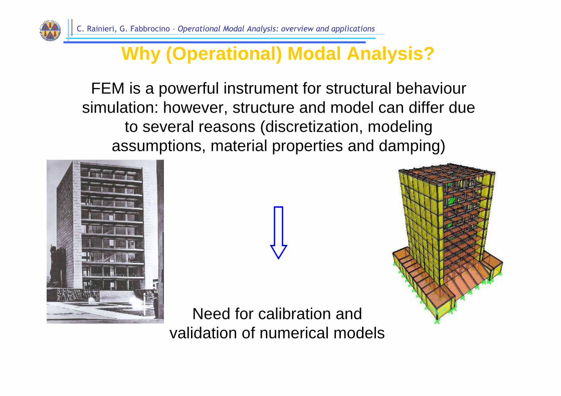
Why (Operational) Modal Analysis?

FEM is a powerful instrument for structural behavioursimulation: however, structure and model can differ due

to several reasons (discretization, modelingassumptions, material properties and damping)

Need for calibration and validation of numerical models


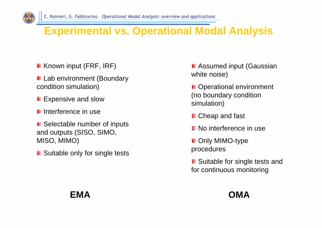
Experimental vs. Operational Modal Analysis

EMA

Known input (FRF, IRF)

Lab environment (Boundarycondition simulation)

Expensive and slow

Interference in use

Selectable number of inputsand outputs (SISO, SIMO, MISO, MIMO)

Suitable only for single tests

Assumed input (Gaussianwhite noise)

Operational environment(no boundary conditionsimulation)

Cheap and fast

No interference in use

Only MIMO-typeprocedures

Suitable for single tests and for continuous monitoring

OMA


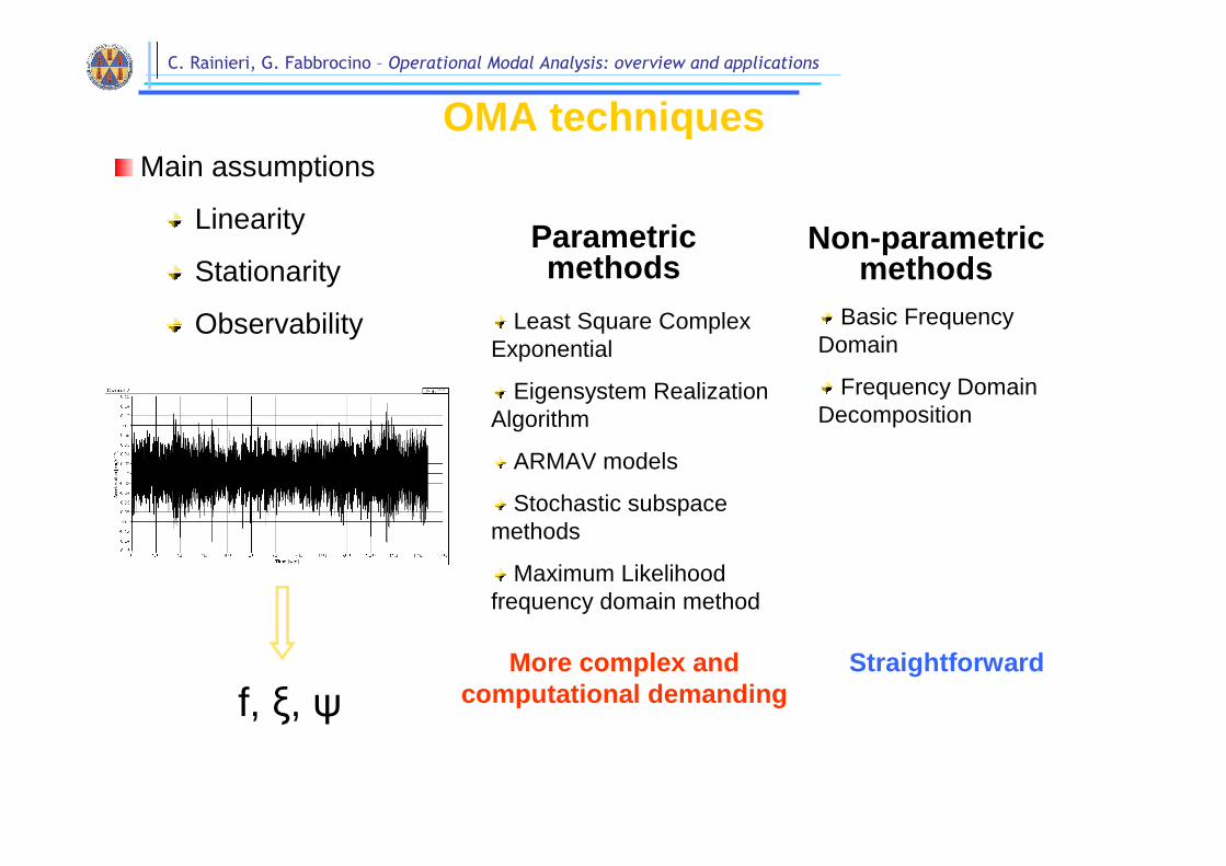
OMA techniques

Non-parametric methods

Parametricmethods

Basic Frequency Domain

Frequency Domain Decomposition

Least Square Complex Exponential

Eigensystem Realization Algorithm

ARMAV models

Stochastic subspace methods

Maximum Likelihood frequency domain method

Main assumptions

Linearity

Stationarity

Observability

StraightforwardMore complex and computational demandingf, ξ, ψ


Easier memory management

Parallelism (simultaneousoperations)

Front Panel = User Interface

Key idea: “from control flow to data flow”

Block Diagram = Code

Communication with hardware

LabView platform


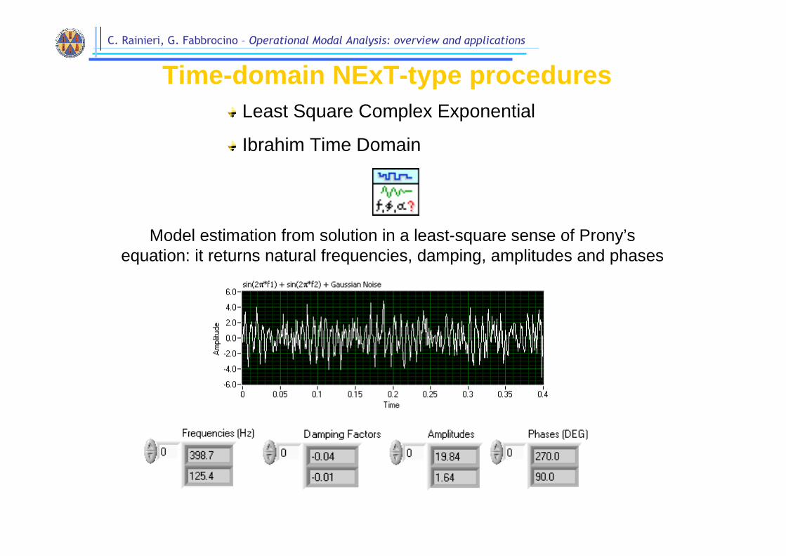
Time-domain NExT-type proceduresLeast Square Complex Exponential

Ibrahim Time Domain

Model estimation from solution in a least-square sense of Prony’s equation: it returns natural frequencies, damping, amplitudes and phases


Time-domain ARMA-type procedures

Optimal model order estimation(Final Prediction Error, Akaike

Information, Bayesian Information, …)

AR, MA and ARMA models

Model estimation


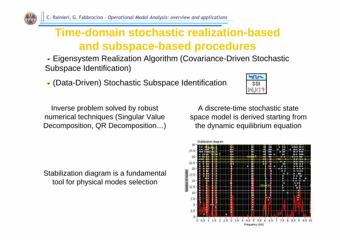
Time-domain stochastic realization-basedand subspace-based procedures

Eigensystem Realization Algorithm (Covariance-Driven Stochastic Subspace Identification)

(Data-Driven) Stochastic Subspace Identification

A discrete-time stochastic state space model is derived starting from

the dynamic equilibrium equation

Inverse problem solved by robustnumerical techniques (Singular ValueDecomposition, QR Decomposition…)

Stabilization diagram is a fundamentaltool for physical modes selection


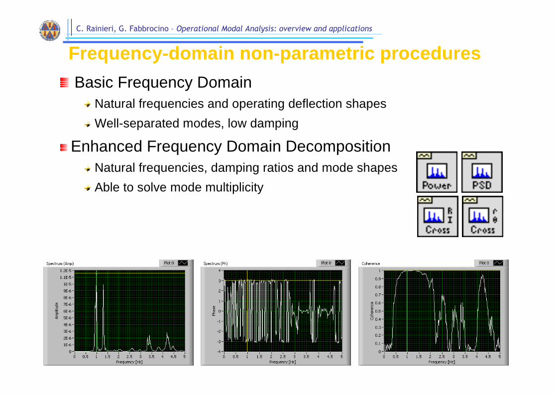
Frequency-domain non-parametric procedures

Basic Frequency DomainNatural frequencies and operating deflection shapes

Well-separated modes, low damping

Enhanced Frequency Domain DecompositionNatural frequencies, damping ratios and mode shapes

Able to solve mode multiplicity


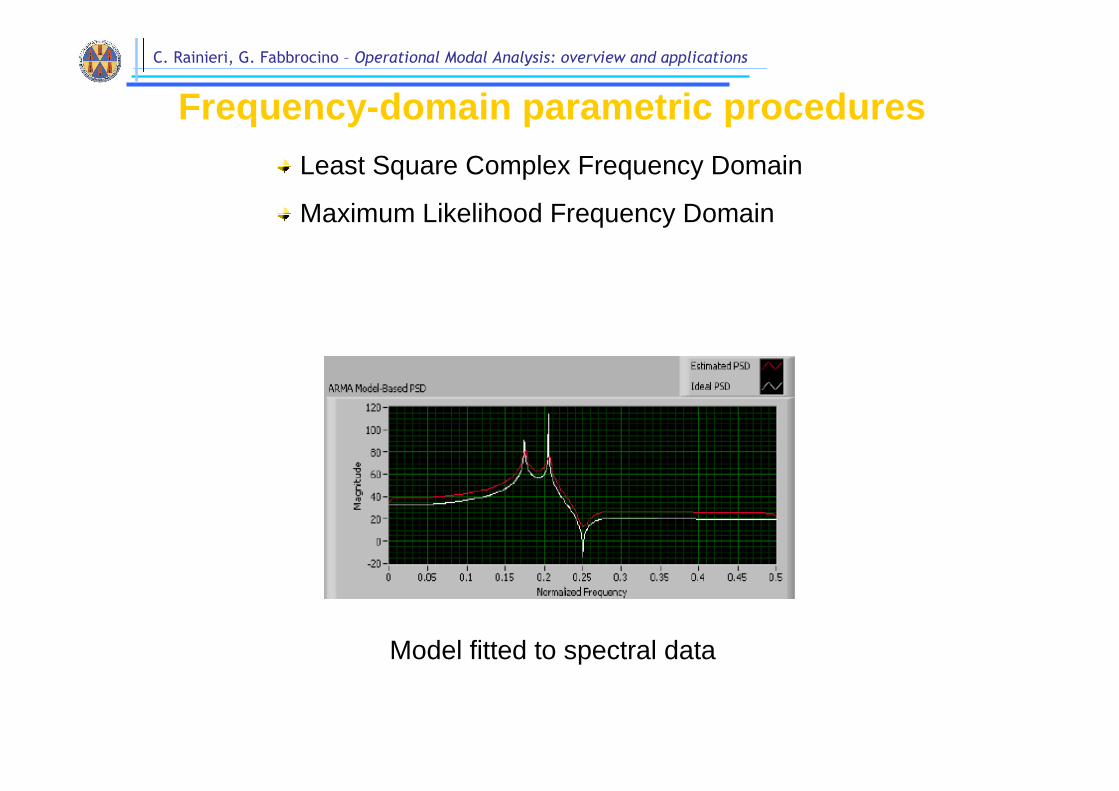
Frequency-domain parametric proceduresLeast Square Complex Frequency Domain

Maximum Likelihood Frequency Domain

Model fitted to spectral data

C. Rainieri – Structural Health Monitoring of relevant structures in seismic regions

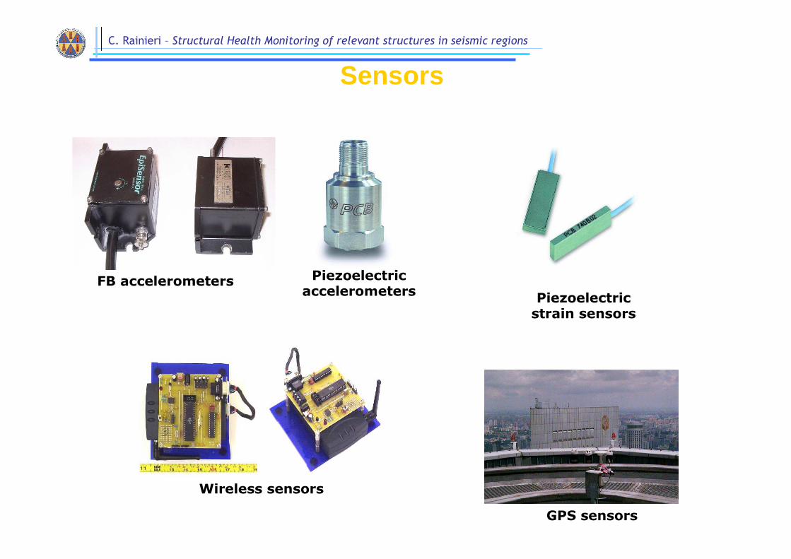
FB accelerometers Piezoelectricaccelerometers

Wireless sensors

GPS sensors

Piezoelectricstrain sensors

Sensors

C. Rainieri – Structural Health Monitoring of relevant structures in seismic regions

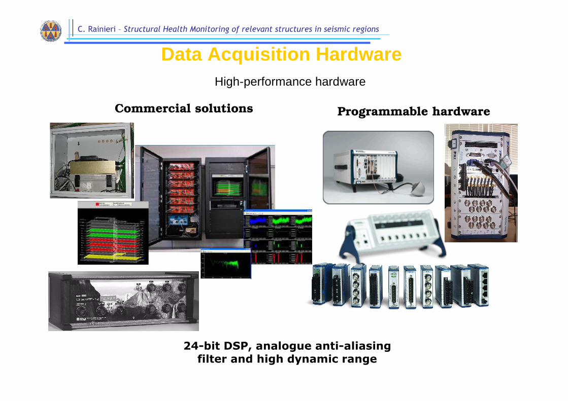
Data Acquisition HardwareHigh-performance hardware

Commercial solutions Programmable hardware

24-bit DSP, analogue anti-aliasing filter and high dynamic range


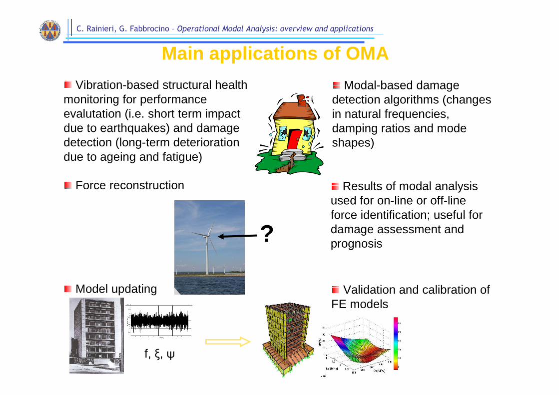
Main applications of OMA

Vibration-based structural healthmonitoring for performance evalutation (i.e. short term impact due to earthquakes) and damagedetection (long-term deteriorationdue to ageing and fatigue)

Modal-based damagedetection algorithms (changesin natural frequencies, damping ratios and mode shapes)

Force reconstruction

Model updating

Results of modal analysisused for on-line or off-line force identification; useful fordamage assessment and prognosis

Validation and calibration of FE models

f, ξ, ψ

?


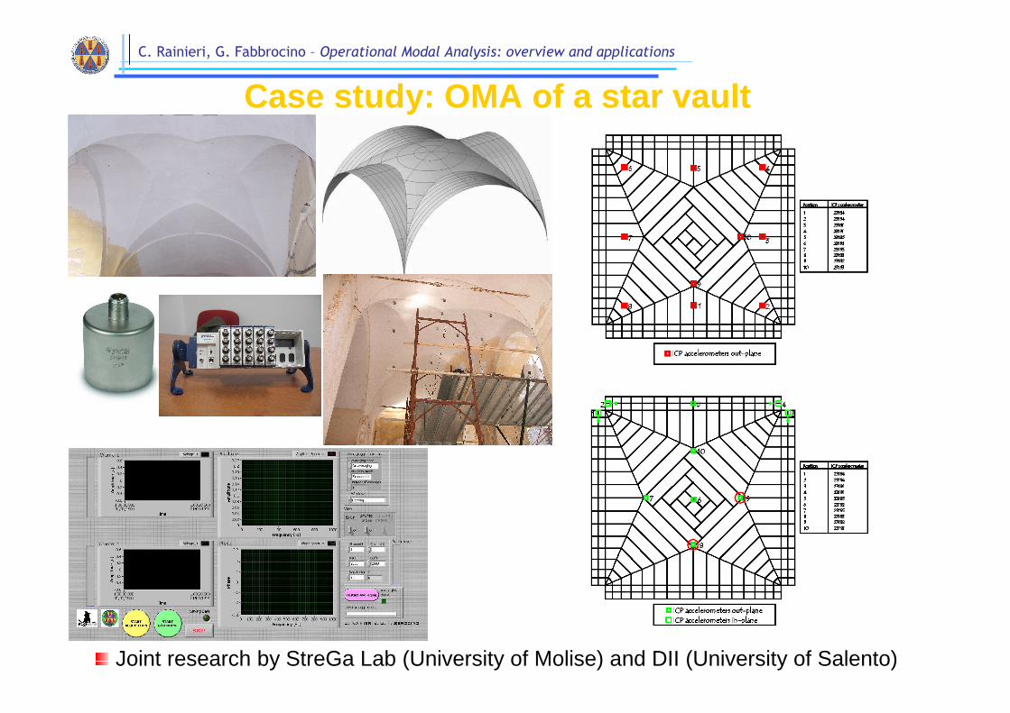
Case study: OMA of a star vault

Joint research by StreGa Lab (University of Molise) and DII (University of Salento)


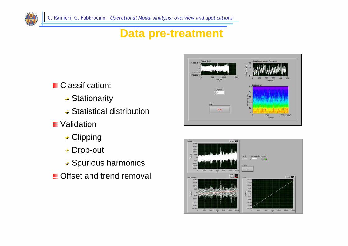
Data pre-treatment

Classification:

Stationarity

Statistical distribution

Validation

Clipping

Drop-out

Spurious harmonics

Offset and trend removal


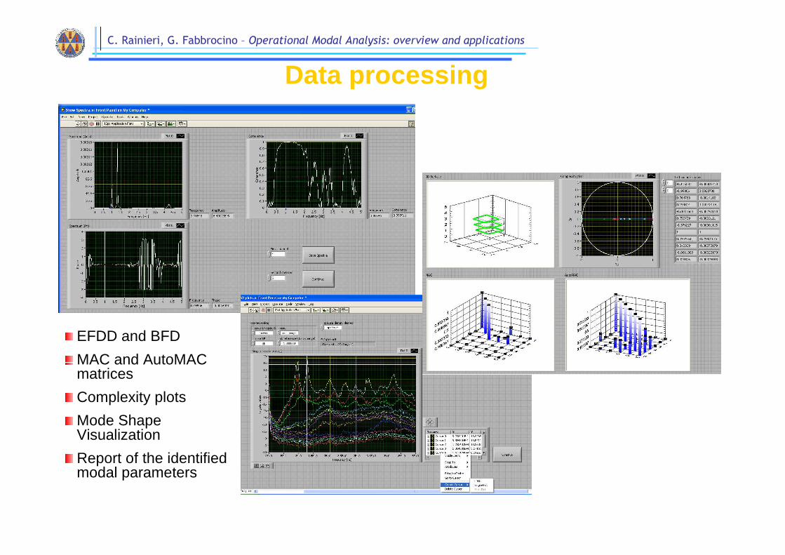
Data processing

EFDD and BFD

MAC and AutoMACmatrices

Complexity plots

Mode ShapeVisualization

Report of the identifiedmodal parameters


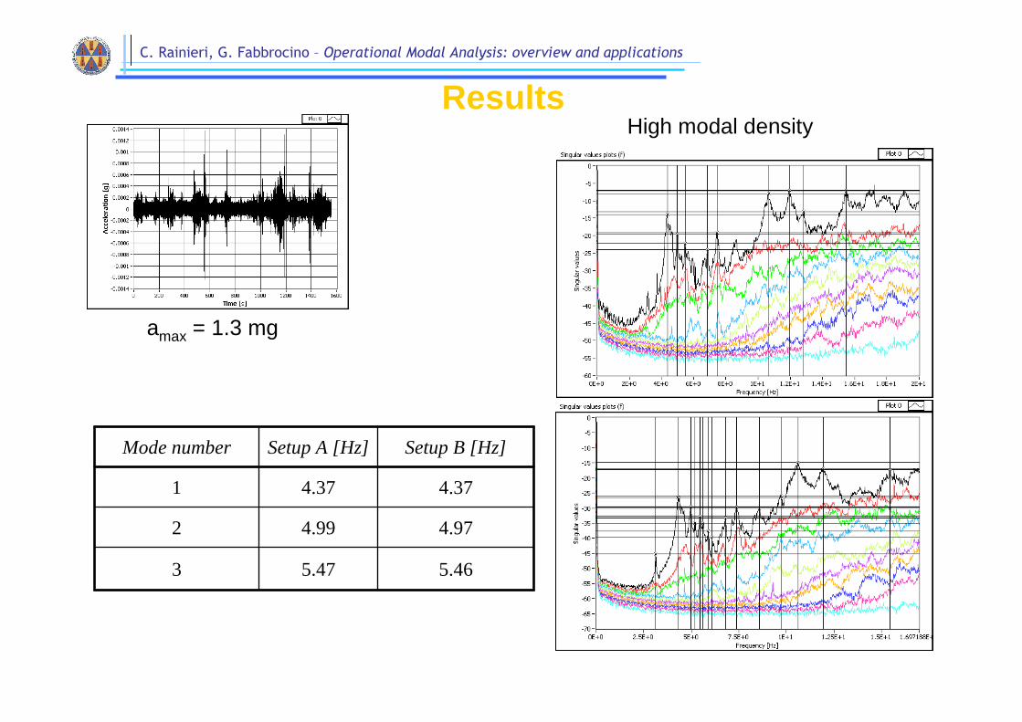
Results

amax = 1.3 mg

High modal density

5.465.473

4.974.992

4.374.371

Setup B [Hz]Setup A [Hz]Mode number


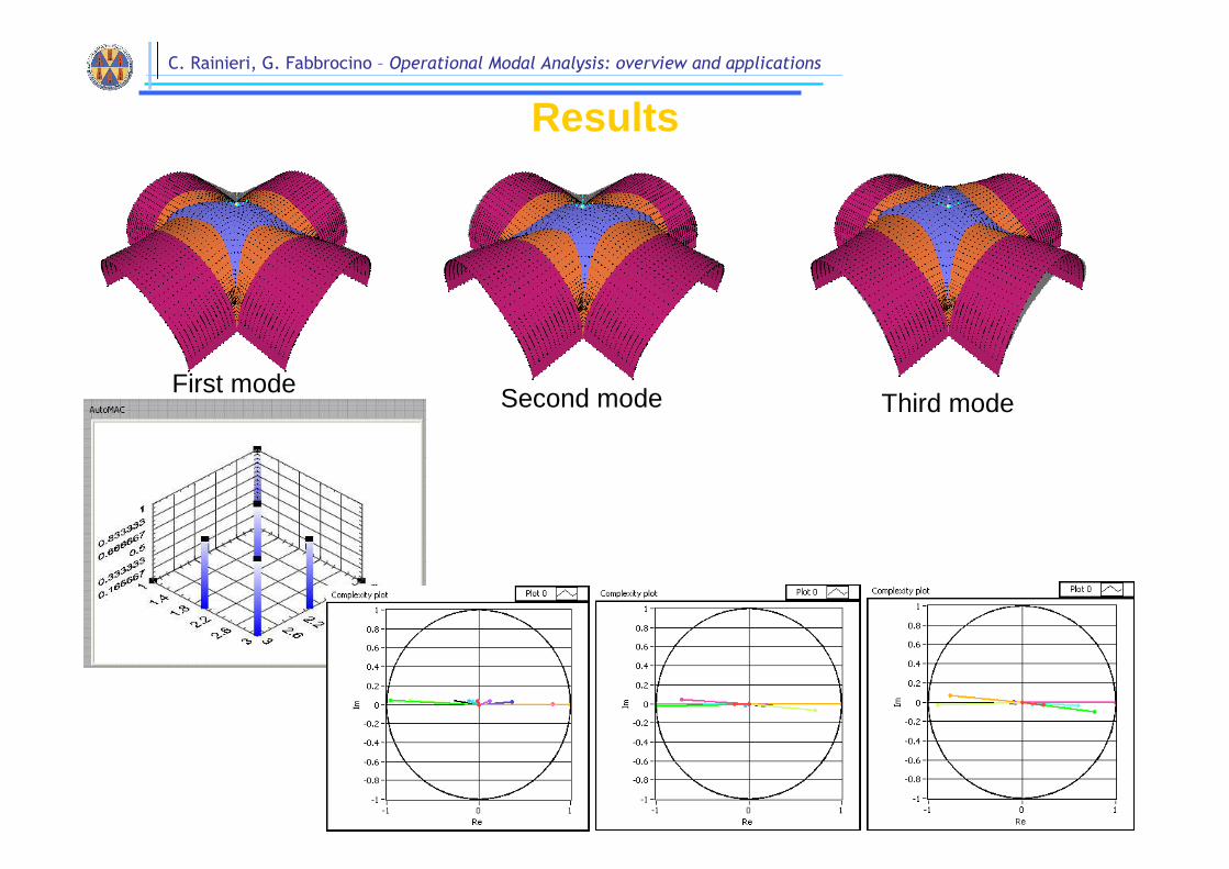
Results

First mode Second mode Third mode


Final remarks and open issues

Operational Modal Analysis is an effective tool for a number of applications

Compared with traditional EMA, it is more versatile, cheaper and faster

Several methods are available in the literature, working both in time and frequency domain

Problems when dealing with harmonics (potential mistakes in mode identification, potential bias in mode estimation, need of a high dynamicrange to extract weak modes in presence of such spurious hamonics)

Un-scaled mode shapes: mass change method for identification of scaling factors

Automation of modal parameter identification techniques for structuralhealth monitoring applications

university of molise engineering faculty - meeting.rgn.hr · university of molise engineering...

Documents