university of newcastle upon tyne - usf …arslan/used_files/matlabtutorial.pdf · university of...
TRANSCRIPT

UNIVERSITY OF NEWCASTLE UPON TYNE
School of Electrical, Electronic and Computer Engineering
Matlab/Simulink Tutorial
Release 13 - version 6.5
Second Edition June 2003

Contents
CHAPTER 1: The Basics ......................................................................................... 1 1.1 Introduction ................................................................................................................ 1 1.2 Simple math............................................................................................................... 2 1.3 Matlab and variables.................................................................................................. 2 1.4 Variables and simple math ........................................................................................ 4 1.5 Complex numbers...................................................................................................... 4 1.6 Common mathematical functions .............................................................................. 5 1.7 M-files ........................................................................................................................ 6 1.8 Workspace................................................................................................................. 8 1.9 Number display formats............................................................................................. 8 1.10 Path Browser ........................................................................................................... 8 1.11 Toolboxes. ............................................................................................................... 8 1.12 Help………............................................................................................................... 8
CHAPTER 2: Arrays and Plots................................................................................ 9 2.1 Array construction...................................................................................................... 9 2.2 Plots ........................................................................................................................... 9 2.3 Array addressing...................................................................................................... 12 2.4 Array Construction ................................................................................................... 14 2.5 Array Orientation...................................................................................................... 16 2.6 Array – Scalar Mathematics .................................................................................... 17 2.7 Array-Array mathematics......................................................................................... 18 2.8 Zeros, Ones, … ....................................................................................................... 19 2.9 Array Manipulation................................................................................................... 20 2.10 Array Searching and Comparison ......................................................................... 21 2.11 Array Size .............................................................................................................. 22 2.12 Matrix operations ................................................................................................... 23
CHAPTER 3: Strings, Logic and Control Flow..................................................... 25 3.1 Strings...................................................................................................................... 25 3.2 Relational and Logical Operations........................................................................... 25
3.2.1 Relational Operators ............................................................................................... 25 3.2.2 Logical Operators.................................................................................................... 26
3.3 Control flow.............................................................................................................. 27 3.3.1 “for” loops................................................................................................................ 27 3.3.2 “while” Loops........................................................................................................... 28 3.3.3 if-else-end Constructions ........................................................................................ 29
CHAPTER 4: Polynomials, Integration & Differentiation .................................... 30 4.1 Polynomials ............................................................................................................. 30 4.2 Numerical Integration............................................................................................... 32 4.3 Numerical Differentiation ......................................................................................... 33 4.4 Functions ................................................................................................................. 34
4.4.1 Rules and Properties .............................................................................................. 34 CHAPTER 5: Introduction to Simulink ................................................................. 36
5.1 Introduction .............................................................................................................. 36 5.2 Solving ODE ............................................................................................................ 36
5.2.1 Example 1............................................................................................................... 39 5.2.2 Example 2............................................................................................................... 43 5.2.3 Example 3............................................................................................................... 45 5.2.4 Exercise .................................................................................................................. 45
5.3 Second Order System Example .............................................................................. 46 5.4 Fourier Spectrum Example...................................................................................... 53

UNIVERSITY OF NEWCASTLE UPON TYNE SCHOOL OF ELECTRICAL, ELECTRONIC AND COMPUTER ENGINEERING
MATLAB BASICS – SECOND EDITION
Chapter 1 Page 1
CHAPTER 1: The Basics
1.1 Introduction
Matlab stands for Matrix Laboratory. The very first version of Matlab, written at the University of New Mexico and Stanford University in the late 1970s was intended for use in Matrix theory, Linear algebra and Numerical analysis. Later and with the addition of several toolboxes the capabilities of Matlab were expanded and today it is a very powerful tool at the hands of an engineer. Typical uses include:
• Math and Computation
• Algorithm development
• Modelling, simulation and prototyping
• Data analysis, exploration and visualisation
• Scientific and engineering graphics
• Application development, including graphical user interface building. Matlab is an interactive system whose basic data element is an ARRAY. Perhaps the easiest way to visualise Matlab is to think it as a full-featured calculator. Like a basic calculator, it does simple math like addition, subtraction, multiplication and division. Like a scientific calculator it handles square roots, complex numbers, logarithms and trigonometric operations such as sine, cosine and tangent. Like a programmable calculator, it can be used to store and retrieve data; you can create, execute and save sequence of commands, also you can make comparisons and control the order in which the commands are executed. And finally as a powerful calculator it allows you to perform matrix algebra, to manipulate polynomials and to plot data. To run Matlab you can either double click on the appropriate icon on the desktop or from the start up menu. When you start Matlab the following window will appear:
Figure 1: Desktop Environment
Initially close all windows except the “Command window”. At the end of these sessions type “Demo” and choose the demo “Desktop Overview” for a full description of all windows. The command window starts automatically with the symbol “>>” In other versions of Matlab this symbol may be different like the educational version: “EDU>>”. When we type a command we press ENTER to execute it.
UNIVERSITY OF NEWCASTLE UPON TYNE SCHOOL OF ELECTRICAL, ELECTRONIC AND COMPUTER ENGINEERING
MATLAB BASICS – SECOND EDITION
Chapter 1 Page 2
1.2 Simple math
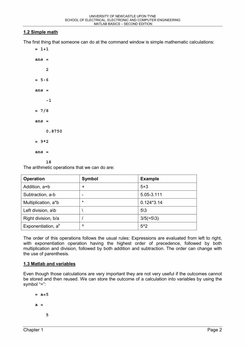
The first thing that someone can do at the command window is simple mathematic calculations: » 1+1
ans =
2
» 5-6
ans =
-1
» 7/8
ans =
0.8750
» 9*2
ans =
18The arithmetic operations that we can do are:
Operation Symbol Example
Addition, a+b + 5+3
Subtraction, a-b - 5.05-3.111
Multiplication, a*b * 0.124*3.14
Left division, a\b \ 5\3
Right division, b/a / 3/5(=5\3)
Exponentiation, ab ^ 5^2 The order of this operations follows the usual rules: Expressions are evaluated from left to right, with exponentiation operation having the highest order of precedence, followed by both multiplication and division, followed by both addition and subtraction. The order can change with the use of parenthesis.
1.3 Matlab and variables
Even though those calculations are very important they are not very useful if the outcomes cannot be stored and then reused. We can store the outcome of a calculation into variables by using the symbol “=”:
» a=5
a =
5
UNIVERSITY OF NEWCASTLE UPON TYNE SCHOOL OF ELECTRICAL, ELECTRONIC AND COMPUTER ENGINEERING
MATLAB BASICS – SECOND EDITION
Chapter 1 Page 3
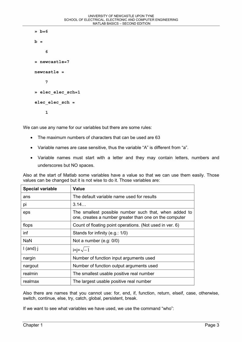
» b=6
b =
6
» newcastle=7
newcastle =
7
» elec_elec_sch=1
elec_elec_sch =
1
We can use any name for our variables but there are some rules:
• The maximum numbers of characters that can be used are 63
• Variable names are case sensitive, thus the variable “A” is different from “a”.
• Variable names must start with a letter and they may contain letters, numbers and
underscores but NO spaces.
Also at the start of Matlab some variables have a value so that we can use them easily. Those values can be changed but it is not wise to do it. Those variables are:
Special variable Value
ans The default variable name used for results
pi 3.14…
eps The smallest possible number such that, when added to one, creates a number greater than one on the computer
flops Count of floating point operations. (Not used in ver. 6)
inf Stands for infinity (e.g.: 1/0)
NaN Not a number (e.g: 0/0)
I (and) j i=j= 1−
nargin Number of function input arguments used
nargout Number of function output arguments used
realmin The smallest usable positive real number
realmax The largest usable positive real number Also there are names that you cannot use: for, end, if, function, return, elseif, case, otherwise, switch, continue, else, try, catch, global, persistent, break. If we want to see what variables we have used, we use the command “who”:
UNIVERSITY OF NEWCASTLE UPON TYNE SCHOOL OF ELECTRICAL, ELECTRONIC AND COMPUTER ENGINEERING
MATLAB BASICS – SECOND EDITION
Chapter 1 Page 4
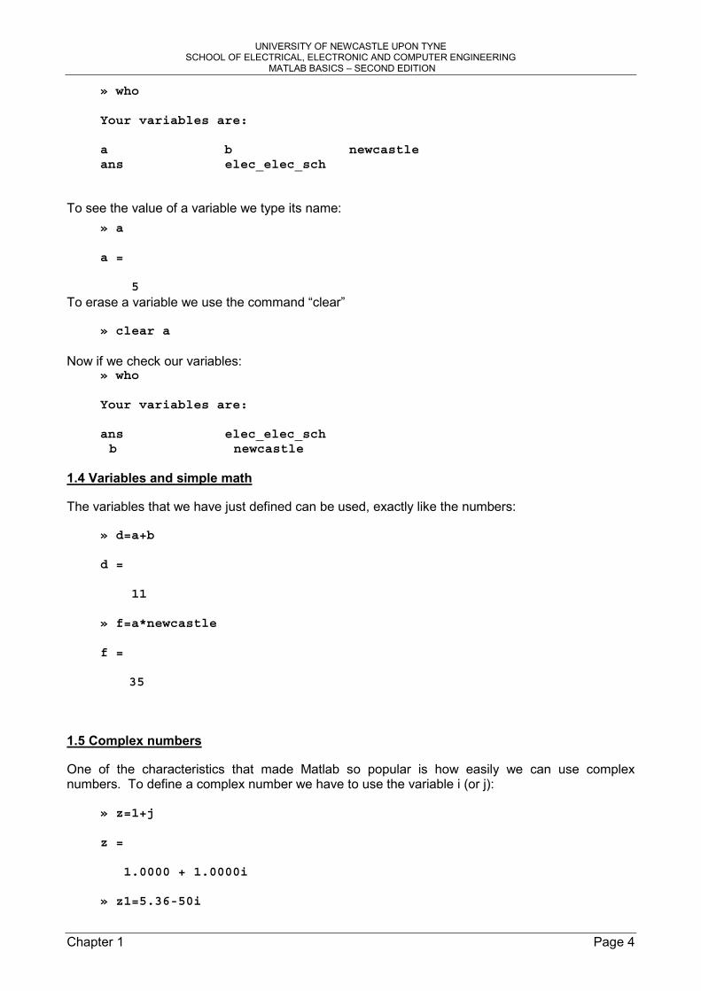
» who
Your variables are:
a b newcastleans elec_elec_sch
To see the value of a variable we type its name: » a
a =
5To erase a variable we use the command “clear”
» clear a Now if we check our variables:
» who
Your variables are:
ans elec_elec_schb newcastle
1.4 Variables and simple math
The variables that we have just defined can be used, exactly like the numbers:
» d=a+b
d =
11
» f=a*newcastle
f =
35
1.5 Complex numbers
One of the characteristics that made Matlab so popular is how easily we can use complex numbers. To define a complex number we have to use the variable i (or j):
» z=1+j
z =
1.0000 + 1.0000i
» z1=5.36-50i
UNIVERSITY OF NEWCASTLE UPON TYNE SCHOOL OF ELECTRICAL, ELECTRONIC AND COMPUTER ENGINEERING
MATLAB BASICS – SECOND EDITION
Chapter 1 Page 5
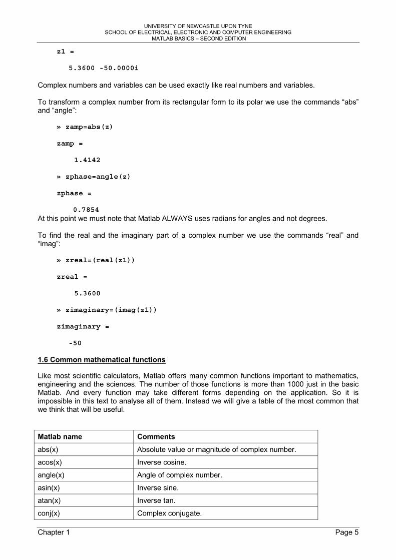
z1 =
5.3600 -50.0000i Complex numbers and variables can be used exactly like real numbers and variables. To transform a complex number from its rectangular form to its polar we use the commands “abs” and “angle”:
» zamp=abs(z)
zamp =
1.4142
» zphase=angle(z)
zphase =
0.7854 At this point we must note that Matlab ALWAYS uses radians for angles and not degrees. To find the real and the imaginary part of a complex number we use the commands “real” and “imag”:
» zreal=(real(z1))
zreal =
5.3600
» zimaginary=(imag(z1))
zimaginary =
-50
1.6 Common mathematical functions
Like most scientific calculators, Matlab offers many common functions important to mathematics, engineering and the sciences. The number of those functions is more than 1000 just in the basic Matlab. And every function may take different forms depending on the application. So it is impossible in this text to analyse all of them. Instead we will give a table of the most common that we think that will be useful.
Matlab name Comments
abs(x) Absolute value or magnitude of complex number.
acos(x) Inverse cosine.
angle(x) Angle of complex number.
asin(x) Inverse sine.
atan(x) Inverse tan.
conj(x) Complex conjugate.
UNIVERSITY OF NEWCASTLE UPON TYNE SCHOOL OF ELECTRICAL, ELECTRONIC AND COMPUTER ENGINEERING
MATLAB BASICS – SECOND EDITION
Chapter 1 Page 6
cos(x) Cosine.
exp(x) ex.
imag(x) Complex imaginary part.
log(x) Natural logarithm.
log10(x) Common logarithm.
real(x) Complex real part.
rem(x,y) Remainder after division: x/y
round(x) Round toward nearest integer.
sqrt(x) Square root.
tan(x) Tangent
One useful operation of the command prompt is that we can recall previous commands by using the cursor keys (↑,↓). Also with the use of the mouse we can copy and paste commands.
1.7 M-files
For simple problems, entering the commands at the Matlab prompt is fast and efficient. However as the number of commands increases, or when you wish to change the value of a variable and then re-valuate all the other variables, typing at the command prompt is tedious. Matlab provides for this a logical solution: place all your commands in a text file and then tell Matlab to evaluate those commands. These files are called script files or simple M-files. To create an M-file, chose form the File menu the option NEW and then chose M-file. Or click at the appropriate icon at the command window. Then you will see this window:
Figure 2: M-file window
After you type your commands save the file with an appropriate name in the directory “work”. Then to run it go at the command prompt and simple type its name or in the M-file window press F5. Be careful if you name your file with a name that has also used for a variable, Matlab is going to give you the value of that variable and not run the M-file. When you run the M-file you will not see the commands (unless you would like to) but only the outcomes of the calculations. If you want to do a calculation either at the command prompt or in an M-file but not to see the outcome you must use

UNIVERSITY OF NEWCASTLE UPON TYNE SCHOOL OF ELECTRICAL, ELECTRONIC AND COMPUTER ENGINEERING
MATLAB BASICS – SECOND EDITION
Chapter 1 Page 7
the symbol “;” at the end of the command. This is very useful and makes the program very fast. E.g.:
» a=10
a =
10
» b=5
b =
5
» c=a+b
c =
15 With this code you actually want only the value of the variable “c” and not “a” and “b” so:
» a=10;» b=5;» c=a+b
c =
15 Even though now this seems a littlie bit unnecessary you will find it imperative with more complex programs. Because of the utility of M-files, Matlab provides several functions that are particularly useful: Matlab name Comments
disp(ans) Display results without identifying the variable names
disp(‘Text’) Display Text
input Prompt user for input
keyboard Give control to keyboard temporally. (type return to quit)
pause Pause until user presses any keyboard key
pause(n) Pause for n seconds
waitforbuttonpress Pause until user presses mouse button or keyboard key. When you write an M-file it is useful to put commends after every command. To do this use the symbol “%”:
temperature=30 % set the temperaturetemperature =
30
UNIVERSITY OF NEWCASTLE UPON TYNE SCHOOL OF ELECTRICAL, ELECTRONIC AND COMPUTER ENGINEERING
MATLAB BASICS – SECOND EDITION
Chapter 1 Page 8
1.8 Workspace
All the variables that you have used either at the command prompt or at an M-file are stored in the Matlab workspace. But if you type the command “clear” or you exit Matlab all these are lost. If you want to keep them you have to save them in “mat” files. To do this go from the File menu to the option: “save workspace as…”. Then save it as the directory “work”. So the next time you would like to use those variables you will load this “mat” file. To do this go at the File menu at chose “Load workspace…”. To see the workspace except from the command who (or whos) you can click at the appropriate icon at the command window.
1.9 Number display formats
When Matlab displays numerical results it follows some rules. By default, if a result is an integer, Matlab displays it as an integer. Likewise, when a result is a real number, Matlab displays it with approximately four digits to the right of the decimal point. You can override this default behaviour by specifying a different numerical format within the preferences menu item in the File menu. The most common formats are the short (default), which shows four digits, and the format long, which shows 15 digits. Be careful in the memory the value is always the same. Only the display format we can change.
1.10 Path Browser
Until now we keep say save the M-file or the workspace to the “work” directory. You can change this by changing the Matlab path. To see the current path type the command “path”. If you wish to change the path (usually to add more directories) from the File menu chose “Set Path…”. The Following window will appear:
Figure 3 Path Browser
After you added a directory you have to save the new path if you want to keep it for future uses.
1.11 Toolboxes.
To expand the possibilities of Matlab there are many libraries that contain relevant functions. Those libraries are called Toolboxes. Unfortunately because of the volume of those toolboxes it is impossible to describe all of these now.
1.12 Help………..
As you have realised until now Matlab can be very complicated. For this reason Matlab provides two kinds of help. The first one is the immediately help. When you want to see how to use a command type “help commandname”. Then you will see a small description about this command. The second way to get help is to get to from the help menu in the command window.

UNIVERSITY OF NEWCASTLE UPON TYNE SCHOOL OF ELECTRICAL, ELECTRONIC AND COMPUTER ENGINEERING
MATLAB BASICS
Chapter 2 Page 9
CHAPTER 2: Arrays and Plots
2.1 Array construction
Consider the problem of computing values of the sine function over one half of its period, namely: y=sin(x), x E [0,π]. Since it is impossible to compute sin(x) at all points over this range (there are infinite number of points), we must choose a finite number of points. In doing so, we are sampling the function. To pick some number, let’s say evaluate every 0.1π in this range, i.e. let x={0, 0.1π, 0.2π, 0.3π, 0.4π, 0.5π, 0.6π, 0.7π, 0.8π, 0.9π, π}. In Matlab to create this vector is relative easy:
» x=[0 0.1*pi 0.2*pi 0.3*pi 0.4*pi 0.5*pi 0.6*pi 0.7*pi 0.8*pi0.9*pi pi]
x =
Columns 1 through 7
0 0.3142 0.6283 0.9425 1.2566 1.5708 1.8850
Columns 8 through 11
2.1991 2.5133 2.8274 3.1416 To evaluate the function y at this points we type:
» y=sin(x)
y =
Columns 1 through 7
0 0.3090 0.5878 0.8090 0.9511 1.0000 0.9511
Columns 8 through 11
0.8090 0.5878 0.3090 0.0000
To create an array in Matlab, all you have to do is to start with a left bracket enter the desired values separated by comas or spaces, then close the array with a right bracket. Notice how Matlab finds the values for “x” and stores them in the array “y”.
2.2 Plots
One of the most useful abilities of Matlab is the ease of plotting data. In Matlab we can plot two and three-dimensional graphics. Here we will only study two-dimensional plots. Assume that in vector “x” we have the data from an experiment. To plot those we use the command “plot” like this:
» z=rand(1,100);» plot(z)
Then we will see a new window that contains the following figure:

UNIVERSITY OF NEWCASTLE UPON TYNE SCHOOL OF ELECTRICAL, ELECTRONIC AND COMPUTER ENGINEERING
MATLAB BASICS
Chapter 2 Page 10
0 10 20 30 40 50 60 70 80 90 1000
0.1
0.2
0.3
0.4
0.5
0.6
0.7
0.8
0.9
1
As we can see the command “plot” created a graph where the elements of the “y” axis are the values of the vector “z” and at the ”x” axis we have the number of the index inside the vector.
Another way to use the command “plot” is like this: » t=0:0.1:10;» z=sin(2*pi*t);» plot(t,z)
0 1 2 3 4 5 6 7 8 9 10-1
-0.8
-0.6
-0.4
-0.2
0
0.2
0.4
0.6
0.8
1
Also we can combine two graphs at the same figure:
» t=0:0.1:10;» z1=sin(2*pi*t);» z2=cos(2*pi*t);» plot(t,z1,t,z2)
0 1 2 3 4 5 6 7 8 9 10-1
-0.8
-0.6
-0.4
-0.2
0
0.2
0.4
0.6
0.8
1
UNIVERSITY OF NEWCASTLE UPON TYNE SCHOOL OF ELECTRICAL, ELECTRONIC AND COMPUTER ENGINEERING
MATLAB BASICS
Chapter 2 Page 11
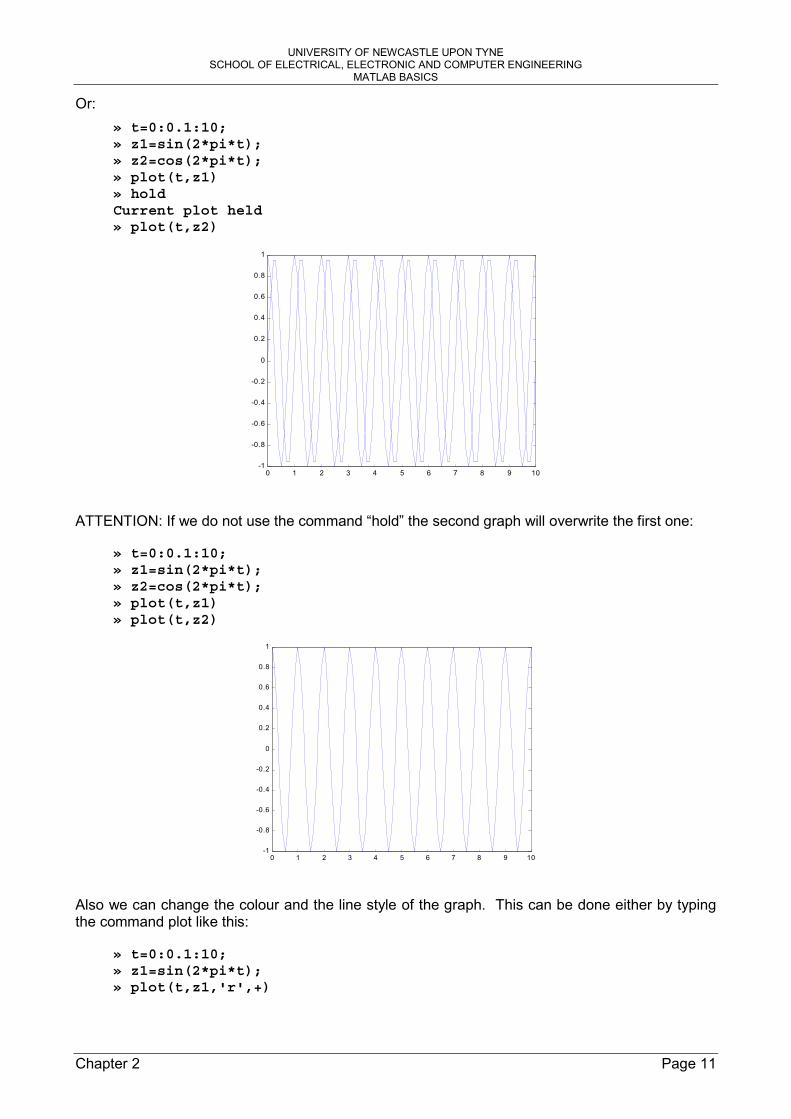
Or: » t=0:0.1:10;» z1=sin(2*pi*t);» z2=cos(2*pi*t);» plot(t,z1)» holdCurrent plot held» plot(t,z2)
0 1 2 3 4 5 6 7 8 9 10-1
-0.8
-0.6
-0.4
-0.2
0
0.2
0.4
0.6
0.8
1
ATTENTION: If we do not use the command “hold” the second graph will overwrite the first one:
» t=0:0.1:10;» z1=sin(2*pi*t);» z2=cos(2*pi*t);» plot(t,z1)» plot(t,z2)
0 1 2 3 4 5 6 7 8 9 10-1
-0.8
-0.6
-0.4
-0.2
0
0.2
0.4
0.6
0.8
1
Also we can change the colour and the line style of the graph. This can be done either by typing the command plot like this:
» t=0:0.1:10;» z1=sin(2*pi*t);» plot(t,z1,'r',+)

UNIVERSITY OF NEWCASTLE UPON TYNE SCHOOL OF ELECTRICAL, ELECTRONIC AND COMPUTER ENGINEERING
MATLAB BASICS
Chapter 2 Page 12
0 1 2 3 4 5 6 7 8 9 10-1
-0.8
-0.6
-0.4
-0.2
0
0.2
0.4
0.6
0.8
1
Or after the plot has been created by double clicking on the graph.
Finally to insert a figure in “Word” we chose from the menu “Edit” the “Copy Figure” choice:
And then simply “paste” on the “Word” file.
2.3 Array addressing
Suppose that we have the array “x” and we want to find the value of the third element. To do this we type:
» a=x(3)
a =
0.6283

UNIVERSITY OF NEWCASTLE UPON TYNE SCHOOL OF ELECTRICAL, ELECTRONIC AND COMPUTER ENGINEERING
MATLAB BASICS
Chapter 2 Page 13
Or we want the first five elements:
» b=x(1:5)
b =
0 0.3142 0.6283 0.9425 1.2566 Notice that, in the first case the variable “a” is a scalar variable and at the second the variable “b” is a vector. Also if we want the elements from the seventh and after we type:
» c=x(7:end)
c =
1.8850 2.1991 2.5133 2.8274 3.1416 Here the word “end” specifies the last element of the array “x”. There are many other ways to address:
» d=y(3:-1:1)
d =
0.5878 0.3090 0 These are the third, second and first element in reverse order. The term 3:-1:1 says “start with 3, count down by 1 and stop at 1. Or:
» e=x(2:2:7)
e =
0.3142 0.9425 1.5708 These are the second, fourth and sixth element of x. The term 2:2:7 says, ”start with 2 count up by two and stop when seven”. In this case adding 2 to 6 gives 8, which is greater than 7, so the eighth element is not included.
Or:» f=y([8 2 9 1])
f =
0.8090 0.3090 0.5878 0
Here we used the array [8 2 9 1] to extract the elements of the array “y” in the order we want them.

UNIVERSITY OF NEWCASTLE UPON TYNE SCHOOL OF ELECTRICAL, ELECTRONIC AND COMPUTER ENGINEERING
MATLAB BASICS
Chapter 2 Page 14
2.4 Array Construction
Earlier we entered the values of “x” by typing each individual element in “x”. While this is fine when there are only 11 values of “x”, what if there are 111 values? So we need a way to automatically generate an array.
This is:
» x=(0:0.1:1)*pi
x =
Columns 1 through 7
0 0.3142 0.6283 0.9425 1.2566 1.5708 1.8850
Columns 8 through 11
2.1991 2.5133 2.8274 3.1416
Or:
» x=[0:0.1:1]*pi
x =
Columns 1 through 7
0 0.3142 0.6283 0.9425 1.2566 1.5708 1.8850
Columns 8 through 11
2.1991 2.5133 2.8274 3.1416
The second way is not very good because it takes longer for Matlab to calculate the outcome (see [2] page 42).
Or:» x=(0:0.1:1)
x =
Columns 1 through 7
0 0.1000 0.2000 0.3000 0.4000 0.5000 0.6000
Columns 8 through 11
0.7000 0.8000 0.9000 1.0000
» xa=x*pi
xa =
Columns 1 through 7

UNIVERSITY OF NEWCASTLE UPON TYNE SCHOOL OF ELECTRICAL, ELECTRONIC AND COMPUTER ENGINEERING
MATLAB BASICS
Chapter 2 Page 15
0 0.3142 0.6283 0.9425 1.2566 1.5708 1.8850
Columns 8 through 11
2.1991 2.5133 2.8274 3.1416
Or we can use the command “linspace”:
» x=linspace(0,pi,11)
x =
Columns 1 through 7
0 0.3142 0.6283 0.9425 1.2566 1.5708 1.8850
Columns 8 through 11
2.1991 2.5133 2.8274 3.1416
In the first cases the notation “0:0.1:1” creates an array that starts at 0, increments by 0.1 and ends at 1. Each element then is multiplied by π to create the desire values in “x”. In the second case, the Matlab function “linspace” is used to create “x”. This function’s arguments are described by: linspace(first_value, last_value, number_of_values)
The first notation allows you to specify the increment between data points, but not the number of the data points. “linspace”, on the other hand, allows you to specify directly the number of the data points, but not the increment between the data points. For the special case where a logarithmically spaced array is desired, Matlab provides the “logspace” function:
» a=logspace(0,2,11)
a =
Columns 1 through 7
1.0000 1.5849 2.5119 3.9811 6.3096 10.000015.8489
Columns 8 through 11
25.1189 39.8107 63.0957 100.0000
Here the array starts with 100, ending at 102 and contains 11 values.
Also Matlab provides the possibility to combine the above methods:
» a=1:5
a =

UNIVERSITY OF NEWCASTLE UPON TYNE SCHOOL OF ELECTRICAL, ELECTRONIC AND COMPUTER ENGINEERING
MATLAB BASICS
Chapter 2 Page 16
1 2 3 4 5
» b=1:2:9
b =
1 3 5 7 9
» c=[a b]
c =
1 2 3 4 5 1 3 5 7 9
2.5 Array Orientation
In the preceding examples, arrays contained one row and multiple columns. As a result of this row orientation, they are commonly called row vectors. It is also possible to have a column vector, having one column and multiple rows. In this case, all of the above array manipulation and mathematics apply without change. The only difference is that results are displayed as columns, rather than as rows. To create a column vector we use the symbol “;”:
» c=[1;2;3;4]
c =
1234
So while spaces (and commas) separate columns, semicolons separate rows. Another way to create a column vector is to make a row vector and then to transpose it:
» x=linspace(0,pi,11);
» x1=x'
x1 =
00.31420.62830.94251.25661.57081.88502.19912.51332.82743.1416
If the vector x contained complex numbers then the operator “’” would also give the conjugate of the elements:

UNIVERSITY OF NEWCASTLE UPON TYNE SCHOOL OF ELECTRICAL, ELECTRONIC AND COMPUTER ENGINEERING
MATLAB BASICS
Chapter 2 Page 17
» k=[0 1+2i 3+0.5465i];» l=k'
l =
01.0000 - 2.0000i3.0000 - 0.5465i
To avoid this we can use the dot-transpose:» l=k.'
l =
01.0000 + 2.0000i3.0000 + 0.5465i
Since we can make column and row vectors is it possible to combine them and to make a matrix? The answer is yes. By using spaces (or commas) to separate columns and semicolons to separate rows:
» A=[1 2 3; 4 5 6]
A =
1 2 34 5 6
Or we can use the following notation:
» A=[1 2 34 5 6]
A =
1 2 34 5 6
2.6 Array – Scalar Mathematics
When we use scalar and arrays we have to be careful. For example the expression g-2, where g is a matrix would mean g-2*I, where “I” is the unitary matrix. In Matlab this does not apply. The above expression would mean subtract from all the elements in the matrix g the number 2.:
» g=[1 2 3;4 5 6];» g1=g-2
g1 =
-1 0 12 3 4
Otherwise we can do everything that we can do with the scalar variables.

UNIVERSITY OF NEWCASTLE UPON TYNE SCHOOL OF ELECTRICAL, ELECTRONIC AND COMPUTER ENGINEERING
MATLAB BASICS
Chapter 2 Page 18
2.7 Array-Array mathematics
Here we can do any operation we want as long as it is mathematically correct. For example we cannot add matrices that have different number of rows and columns.
» A=[1 2 3 4;5 6 7 8;9 10 11 12];» B=[1 1 1 1;2 2 2 2;3 3 3 3];» C=A+B
C =
2 3 4 57 8 9 1012 13 14 15
» D=C-A
D =
1 1 1 12 2 2 23 3 3 3
» F=2*A-D
F =
1 3 5 78 10 12 1415 17 19 21
The multiplication and division with matrices can be done with 2 different ways. The first is the classical “* or /” and follows the laws of the matrix algebra:
» M=[1 2;3 4];» N=[5 6;7 8];» K=M*N
K =
19 2243 50
The second way is to do those arithmetic operations element by element, and so we do need to care about the dimensions of the matrices. To do this we use the symbols “*” and “/” but with a dot in front of them “.*” and “./” :
» K=M.*N
K =
5 1221 32
The same procedure with division and multiplication can be done with array powers:
UNIVERSITY OF NEWCASTLE UPON TYNE SCHOOL OF ELECTRICAL, ELECTRONIC AND COMPUTER ENGINEERING
MATLAB BASICS
Chapter 2 Page 19
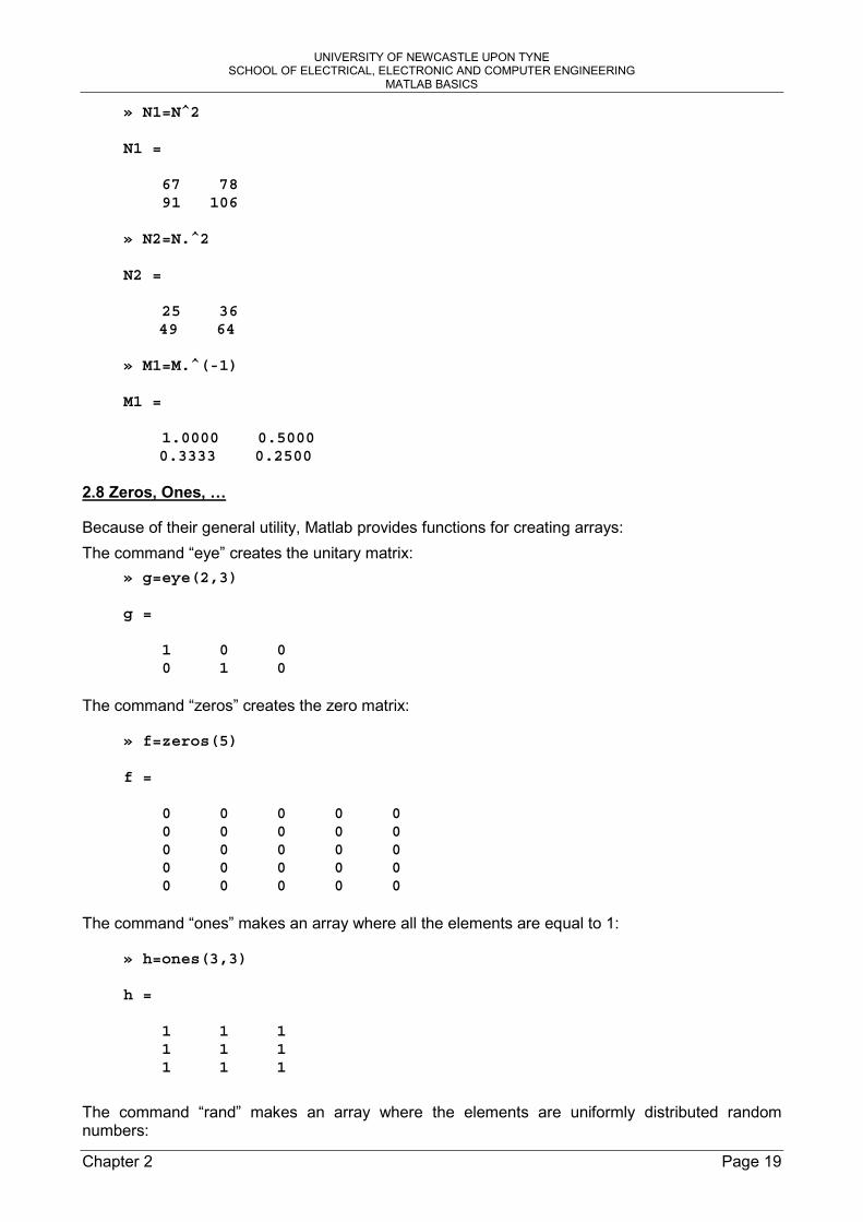
» N1=N^2
N1 =
67 7891 106
» N2=N.^2
N2 =
25 3649 64
» M1=M.^(-1)
M1 =
1.0000 0.50000.3333 0.2500
2.8 Zeros, Ones, …
Because of their general utility, Matlab provides functions for creating arrays: The command “eye” creates the unitary matrix:
» g=eye(2,3)
g =
1 0 00 1 0
The command “zeros” creates the zero matrix:
» f=zeros(5)
f =
0 0 0 0 00 0 0 0 00 0 0 0 00 0 0 0 00 0 0 0 0
The command “ones” makes an array where all the elements are equal to 1:
» h=ones(3,3)
h =
1 1 11 1 11 1 1
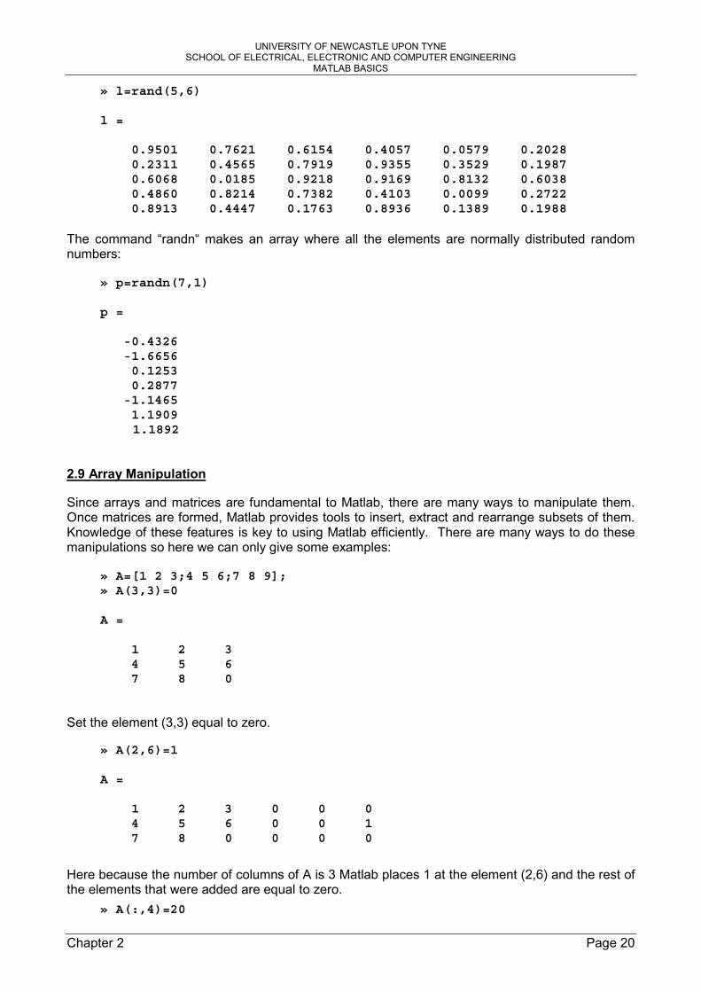
The command “rand” makes an array where the elements are uniformly distributed random numbers:
UNIVERSITY OF NEWCASTLE UPON TYNE SCHOOL OF ELECTRICAL, ELECTRONIC AND COMPUTER ENGINEERING
MATLAB BASICS
Chapter 2 Page 20
» l=rand(5,6)
l =
0.9501 0.7621 0.6154 0.4057 0.0579 0.20280.2311 0.4565 0.7919 0.9355 0.3529 0.19870.6068 0.0185 0.9218 0.9169 0.8132 0.60380.4860 0.8214 0.7382 0.4103 0.0099 0.27220.8913 0.4447 0.1763 0.8936 0.1389 0.1988
The command “randn“ makes an array where all the elements are normally distributed random numbers:
» p=randn(7,1)
p =
-0.4326-1.66560.12530.2877-1.14651.19091.1892
2.9 Array Manipulation
Since arrays and matrices are fundamental to Matlab, there are many ways to manipulate them. Once matrices are formed, Matlab provides tools to insert, extract and rearrange subsets of them. Knowledge of these features is key to using Matlab efficiently. There are many ways to do these manipulations so here we can only give some examples:
» A=[1 2 3;4 5 6;7 8 9];» A(3,3)=0
A =
1 2 34 5 67 8 0
Set the element (3,3) equal to zero.
» A(2,6)=1
A =
1 2 3 0 0 04 5 6 0 0 17 8 0 0 0 0
Here because the number of columns of A is 3 Matlab places 1 at the element (2,6) and the rest of the elements that were added are equal to zero.
» A(:,4)=20

UNIVERSITY OF NEWCASTLE UPON TYNE SCHOOL OF ELECTRICAL, ELECTRONIC AND COMPUTER ENGINEERING
MATLAB BASICS
Chapter 2 Page 21
A =
1 2 3 20 0 04 5 6 20 0 17 8 0 20 0 0
Here Matlab sets all the elements of the fourth column equal to 20.
» A=[1 2 3;4 5 6;7 8 9];
» B=A(3:-1:1,1:3)
B =
7 8 94 5 61 2 3
Here it creates a matrix “B” by taking the rows of “A” in reversed order. The previous manipulation can also be done with the following way:
» B=A(3:-1:1,:)
B =
7 8 94 5 61 2 3
If we want to erase a column then we type:
» A(:,2)=[]
A =
1 34 67 9
If we want to reshape a matrix we type: » A=[1 2 3;4 5 6];
» B=reshape(A,1,6)
B =
1 4 2 5 3 6
2.10 Array Searching and Comparison
Many times, it is desirable to know the indices or subscripts of those elements of an array that satisfy some relational expression. In Matlab, this task is performed by the function “find”, which returns the subscripts where a relational expression is true:
» x=-3:3
x =

UNIVERSITY OF NEWCASTLE UPON TYNE SCHOOL OF ELECTRICAL, ELECTRONIC AND COMPUTER ENGINEERING
MATLAB BASICS
Chapter 2 Page 22
-3 -2 -1 0 1 2 3
» k=find(abs(x)>1)
k =
1 2 6 7 And if we want to find those numbers then:
» y=x(k)
y =
-3 -2 2 3 The command “find” also works with matrices:
» A=[1 2 3;4 5 6;7 8 9];» [i,j]=find(A>5)
i =
3323
j =
1233
At times it is desirable to compare two arrays. For example:
» B=[1 5 6;9 0 0;4 5 1];» A=[1 2 3;4 5 6;7 8 9];» isequal(A,B)
ans =
0
» isequal(A,A)
ans =
1
2.11 Array Size
There are cases where the size of a matrix in unknown but is needed for some manipulation, Matlab provides two utility functions “size” and “length”:

UNIVERSITY OF NEWCASTLE UPON TYNE SCHOOL OF ELECTRICAL, ELECTRONIC AND COMPUTER ENGINEERING
MATLAB BASICS
Chapter 2 Page 23
» A=[1 2 3 4;5 6 7 8];» B=size(A)
B =
2 4
With one output argument, the “size” function returns a row vector whose first element is the number of rows and whose second element is the number of columns.
» [r,c]=size(A)
r =
2
c =
4
With two output arguments, “size” returns the number of rows in the first variable and the number of columns in the second variable. If we want to see which number is bigger (i.e. if the array has more rows than columns) we use the command “length”:
» C=length(A)
C =
4
Actually the function “length” is doing: “max(size(A)”
2.12 Matrix operations
There are various matrix functions that we can do in Matlab, some of them are:
To find the determinant:
» A=[1 2 3;4 5 6;7 8 9];» a=det(A)
a =
0
To find the inverse:» A=[1 5 3;4 5 10;7 8 50];» b=inv(A)
b =
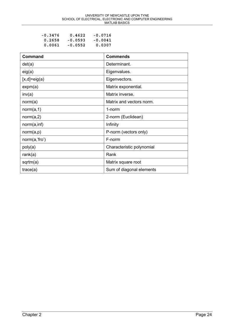
UNIVERSITY OF NEWCASTLE UPON TYNE SCHOOL OF ELECTRICAL, ELECTRONIC AND COMPUTER ENGINEERING
MATLAB BASICS
Chapter 2 Page 24
-0.3476 0.4622 -0.07160.2658 -0.0593 -0.00410.0061 -0.0552 0.0307
Command Commends
det(a) Determinant.
eig(a) Eigenvalues.
[x,d]=eig(a) Eigenvectors.
expm(a) Matrix exponential.
inv(a) Matrix inverse.
norm(a) Matrix and vectors norm.
norm(a,1) 1-norm
norm(a,2) 2-norm (Euclidean)
norm(a,inf) Infinity
norm(a,p) P-norm (vectors only)
norm(a,’fro’) F-norm
poly(a) Characteristic polynomial
rank(a) Rank
sqrtm(a) Matrix square root
trace(a) Sum of diagonal elements

UNIVERSITY OF NEWCASTLE UPON TYNE SCHOOL OF ELECTRICAL, ELECTRONIC AND COMPUTER ENGINEERING
MATLAB BASICS
Chapter 3 Page 25
CHAPTER 3: Strings, Logic and Control Flow
3.1 Strings
The true power of Matlab is its ability to crunch numbers. However it is desirable sometimes to manipulate text. In Matlab, text variables are referred to as character strings, or simple strings. Character strings in Matlab are arrays of ASCII values that are displayed as their character string representation:
» t='how about this character string'
t =
how about this character string
»size(t)ans =1 31
A character string is simple a text surrounded by single quotes.
The function “disp” allows you to display a string without printing its variable name:
» disp(t)how about this character string
3.2 Relational and Logical Operations
3.2.1 Relational Operators Matlab relational operators include:
Relational Operator Description
< Less than
<= Less than or equal to
> Greater than
>= Greater than or equal to
== Equal to
~= Not equal to
General a relational operator returns one for true and zero for false:» A=1:9;» B=9-A;» tf=A>4
tf =
0 0 0 0 1 1 1 1 1

UNIVERSITY OF NEWCASTLE UPON TYNE SCHOOL OF ELECTRICAL, ELECTRONIC AND COMPUTER ENGINEERING
MATLAB BASICS
Chapter 3 Page 26
Here we see that after the fourth element the values of A are greater than 4.» tf=A==B
tf =
0 0 0 0 0 0 0 0 0
Finds element of A that are equal to those of B. The symbol “==” compares two variable and returns one where they are equal and zeros when they are not.
3.2.2 Logical Operators Logical operators provide a way to combine or negate relational expressions. Matlab logical operators include: Logical Operator Description
& AND
| OR
~ NOT
Examples:
» tf=~(A>4)
tf =
1 1 1 1 0 0 0 0 0
» tf=(A>2)&(A<6)
tf =
0 0 1 1 1 0 0 0 0 Other relational and logical operators are: Operator Description
xor(x,y) Exclusive OR operation. Returns ones where either x or y is nonzero (True). Returns zeros if both x and y are zero (False) or nonzero (True)
any(x) Return one if any element of the vector x is nonzero. Return one for each column in a matrix x that has nonzero elements.
all(x) Return one if all elements are nonzero

UNIVERSITY OF NEWCASTLE UPON TYNE SCHOOL OF ELECTRICAL, ELECTRONIC AND COMPUTER ENGINEERING
MATLAB BASICS
Chapter 3 Page 27
3.3 Control flow
3.3.1 “for” loops “for” loops allow a group of commands to be repeated a fixed, predetermined number of times. The general form of a “for” loop is: for x=array
commands…
end
The commands… between the “for” and “end” statements are executed once every column in “array”. At each interaction, “x” is assigned to the next column of “array”, i.e. during the nth time through the loop, x=array.
Example:
» for n=1:10x(n)=sin(n*pi/10);end;» x
x =
Columns 1 through 7
0.3090 0.5878 0.8090 0.9511 1.0000 0.95110.8090
Columns 8 through 10
0.5878 0.3090 0.0000
Also the “for” loops can be nested as desired: clear allfor k=1:10
for l=1:5x(l,k)=5*sqrt(k*l);
end;end;
» x
x =
Columns 1 through 7
5.0000 7.0711 8.6603 10.0000 11.1803 12.247413.2288
7.0711 10.0000 12.2474 14.1421 15.8114 17.320518.7083
8.6603 12.2474 15.0000 17.3205 19.3649 21.213222.9129
10.0000 14.1421 17.3205 20.0000 22.3607 24.494926.4575

UNIVERSITY OF NEWCASTLE UPON TYNE SCHOOL OF ELECTRICAL, ELECTRONIC AND COMPUTER ENGINEERING
MATLAB BASICS
Chapter 3 Page 28
11.1803 15.8114 19.3649 22.3607 25.0000 27.386129.5804
Columns 8 through 10
14.1421 15.0000 15.811420.0000 21.2132 22.360724.4949 25.9808 27.386128.2843 30.0000 31.6228
31.6228 33.5410 35.3553
Sometimes it is possible to avoid “for” loops. This is very good because we make the program faster. For example the first example on this paragraph can be also done:
» n=1:10;» x=sin(n*pi/10)
x =
Columns 1 through 7
0.3090 0.5878 0.8090 0.9511 1.0000 0.95110.8090
Columns 8 through 10
0.5878 0.3090 0.0000
3.3.2 “while” Loops While a “for” loop evaluates a group of commands a fixed number of times, a “while” loop evaluates a group of commands an identified number of times. The general form of a “while” loop is: while expression
Commands
end
The command between the “while” and “end” statements are executed as long as all elements in expression are true. For example:
» a=10;» while a>0y(a)=a*10;a=a-1;end;» y
y =
10 20 30 40 50 60 70 80 90 100
UNIVERSITY OF NEWCASTLE UPON TYNE SCHOOL OF ELECTRICAL, ELECTRONIC AND COMPUTER ENGINEERING
MATLAB BASICS
Chapter 3 Page 29
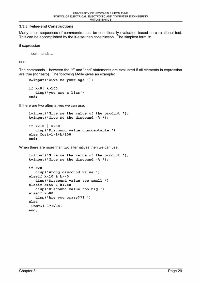
3.3.3 if-else-end Constructions Many times sequences of commands must be conditionally evaluated based on a relational test. This can be accomplished by the if-else-then construction. The simplest form is: if expression
commands…
end
The commands... between the “if” and “end” statements are evaluated if all elements in expression are true (nonzero). The following M-file gives an example:
k=input('Give me your age ');
if k<0| k>100disp('you are a liar')
end;
If there are two alternatives we can use:
l=input('Give me the value of the product ');k=input('Give me the discound (%)');
if k<10 | k>50disp('Discound value unacceptable ')
else Cost=l-l*k/100end;
When there are more than two alternatives then we can use:
l=input('Give me the value of the product ');k=input('Give me the discound (%)');
if k<0disp('Wrong discound value ')
elseif k<10 & k>=0disp('Discound value too small ')
elseif k>50 & k<=80disp('Discound value too big ')
elseif k>80disp('Are you crazy??? ')
elseCost=l-l*k/100
end;

UNIVERSITY OF NEWCASTLE UPON TYNE SCHOOL OF ELECTRICAL, ELECTRONIC AND COMPUTER ENGINEERING
MATLAB BASICS
Chapter 4 Page 30
CHAPTER 4: Polynomials, Integration & Differentiation
4.1 Polynomials
Finding the roots of a polynomial is a problem that arises in many disciplines. Matlab solves this problem and provides other polynomial manipulation tools as well. In Matlab, a polynomial is represented by a row vector of its coefficients in descending order. For example the polynomial
1162512 34 ++− xxx is entered as: » p=[1 -12 0 25 116]
p =
1 -12 0 25 116
Note that terms with zero coefficients must be included.
The roots of a polynomial can be found by the function “roots”:
» q=roots(p)
q =
11.74732.7028-1.2251 + 1.4672i-1.2251 - 1.4672i
If we have the roots we can find the polynomial by using the function “poly”:» p1=poly(q)
p1 =
1.0000 -12.0000 -0.0000 25.0000 116.0000
To multiply two polynomials we use the command “conv”:
» p=[1 -12 0 25 116];» r=[1 1];» pr=conv(p,r)
pr =
1 -11 -12 25 141 116
To divide two polynomials we use the command “deconv”:» a=[1 1 2];» b=[2 0 0 1];» [q,r]=deconv(b,a)
q =

UNIVERSITY OF NEWCASTLE UPON TYNE SCHOOL OF ELECTRICAL, ELECTRONIC AND COMPUTER ENGINEERING
MATLAB BASICS
Chapter 4 Page 31
2 -2
r =
0 0 -2 5
The result says that the quotient of the division is “q” and the remainder is “r”. The differentiation of a polynomial is found by using the function “polyder”:
» pd=polyder(p)
pd =
4 -36 0 2 To evaluate a polynomial at a specific point we use the function “polyval”:
» polyval(p,-1+j)
ans =
63.0000 + 1.0000i
If we have the ratio of two polynomials we manipulate them as two different polynomials:» num=[1 -10 100]; % numerator» den=[1 10 100 0]; % denominator» zeros=roots(num)
zeros =
5.0000 + 8.6603i5.0000 - 8.6603i
» poles=roots(den)
poles =
0-5.0000 + 8.6603i-5.0000 - 8.6603i
But if we want to find the derivative of this ratio we use the command “polyder” in the next form:» [numd,dend]=polyder(num,den)
numd =
-1 20 -100 -2000 -10000
dend =
UNIVERSITY OF NEWCASTLE UPON TYNE SCHOOL OF ELECTRICAL, ELECTRONIC AND COMPUTER ENGINEERING
MATLAB BASICS
Chapter 4 Page 32
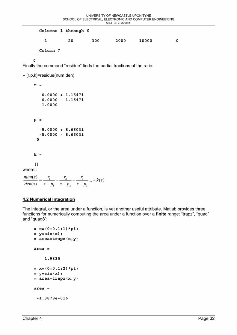
Columns 1 through 6
1 20 300 2000 10000 0
Column 7
0 Finally the command “residue” finds the partial fractions of the ratio:
» [r,p,k]=residue(num,den)
r =
0.0000 + 1.1547i0.0000 - 1.1547i1.0000
p =
-5.0000 + 8.6603i-5.0000 - 8.6603i0
k =
[] where :
)(...)()(
3
3
2
2
1
1 skpsr
psr
psr
sdensnum +
−+
−+
−=
4.2 Numerical Integration
The integral, or the area under a function, is yet another useful attribute. Matlab provides three functions for numerically computing the area under a function over a finite range: “trapz”, “quad” and “quad8”:
» x=(0:0.1:1)*pi;» y=sin(x);» area=trapz(x,y)
area =
1.9835
» x=(0:0.1:2)*pi;» y=sin(x);» area=trapz(x,y)
area =
-1.3878e-016

UNIVERSITY OF NEWCASTLE UPON TYNE SCHOOL OF ELECTRICAL, ELECTRONIC AND COMPUTER ENGINEERING
MATLAB BASICS
Chapter 4 Page 33
The function “trapz’ approximates the area under the function “sin” as trapezoids. If we want better approximation we have to reduce the size of those trapezoids. We can clearly see that, this approximation calculation inserts an error. This is obvious in the second example where the “area” is equal to a very small number but not to zero. The functions “quad” and “quad8” are used in a different format and give better approximation than trapz:
» area=quad('sin',0,2*pi)
area =
0
4.3 Numerical Differentiation
Compared to integration, numerical differentiation is much more difficult. Integration describes an overall or macroscopic property of a function, whereas differentiation describes the slope of a function at a point, which is a microscopic property of a function. As a result, integration is not sensitive to minor changes in the shape of a function, whereas differentiation is. Any small changes in a function can easily create large changes in its slope in the neighbourhood of the change. Because of this inherent difficulty with differentiation, numerical differentiation is avoided wherever it is possible, especially if the data are obtained experimentally. In this case it is best to perform a least squares curve fit to data and then find the resulting polynomial. To find a polynomial that fits at a set of data we use the command “polyfit(x,y,n)”, where “x” are the data of the x-axis, “y” are the data for the y-axis and “n” are the order of the polynomial that we want to fit. So to find the derivative at a specific point we use:
» x=0:0.1:1;» y=[-0.447 1.978 3.28 6.16 7.08 7.34 7.66 9.56 9.48 9.30 11.2];» p=polyfit(x,y,2)
p =
-9.8108 20.1293 -0.0317
» pd=polyder(p)
pd =
-19.6217 20.1293
» slope_of_p=polyval(pd,0.5)
slope_of_p =
10.3185
Matlab provides on the other hand a function that computes, very rough, the derivative of the data that describe a function. This is the function “diff” :
» dy=diff(y)./diff(x)
dy =
UNIVERSITY OF NEWCASTLE UPON TYNE SCHOOL OF ELECTRICAL, ELECTRONIC AND COMPUTER ENGINEERING
MATLAB BASICS
Chapter 4 Page 34
Columns 1 through 7
24.2500 13.0200 28.8000 9.2000 2.6000 3.200019.0000
Columns 8 through 10
-0.8000 -1.8000 19.0000
Note the last function is well to be avoided and to be used only when it is necessary.
4.4 Functions
When you use in Matlab functions such as: “inv”, “abs”, “angle”… Matlab takes the variables you pass it, computes the required results using your input, and then passes those results back to you. Functions are a very powerful tool inside Matlab and can reduce the size and the complexity of a program. The next example helps us to understand the use of functions: Suppose we want to add two arrays and give back only the outcome. To do this we need as inputs the two arrays and as output Matlab will return the sum. We chose the name of our function as “fun1”. We go to the same place as the M-file and we type:
function z=fun1(x,y)% This is a demo% of how to use functions% This function finds the sum of two matrices (x,y)% and stores the outcome at the matrix "z"
z=x+y;
Later at the command prompt we type:
» a=[1 1;2 2];» b=[3 3;4 4];» outcome=fun1(a,b)
outcome =
4 46 6If we want to see the help of this function we type:
» help fun1
This is a demoof how to use functionsThis function finds the sum of two matrices (x,y)and stores the outcome at the matrix "z"
4.4.1 Rules and Properties 1) The function name and file name are IDENTICAL. 2) Comment lines up to the first noncomment line in a function M-file are the help text
returned when you request help.
UNIVERSITY OF NEWCASTLE UPON TYNE SCHOOL OF ELECTRICAL, ELECTRONIC AND COMPUTER ENGINEERING
MATLAB BASICS
Chapter 4 Page 35
3) Each function has each own workspace separate from the Matlab workspace. The only connections between the variables within a function and the Matlab workspace are the function’s input and output variables. If a function changes the value of a variable this appear only inside the function. If a variable is created inside a function does NOT appear at the Matlab workspace.
4) Functions can share the same variables if we use the command “global”:
function z=fun1(x,y)% This is a demo% of how to use functions% This function finds the sum of two matrices (x,y)% and stores the outcome at the matrix "z"
global g1;g1=10;z=x+y;
function z=fun2(x)% This is a demo% of how to use functions% This function finds the product of a matrix and% the global variable g1% and stores the outcome at the matrix "z"global g1z=g1*x;» outcome1=fun2(a)outcome1 =
10 1020 20
Finally inside a function can be used other functions as well:
function z=fun3(x)% This is a demo% of how to use functions% This function finds the product of a matrix and% the global variable g1, then it finds the square root of the% elements% and stores the outcome at the matrix "z"global g1z1=g1*x;z=sqrt(z1);
» outcome2=fun3(a)
outcome2 =
3.1623 3.16234.4721 4.4721
UNIVERSITY OF NEWCASTLE UPON TYNE SCHOOL OF ELECTRICAL, ELECTRONIC AND COMPUTER ENGINEERING
MATLAB BASICS
Chapter 5 Page 36
CHAPTER 5: Introduction to Simulink
5.1 Introduction
Simulink is a time based software package that is included in Matlab and its main task is to solve Ordinary Differential Equations (ODE) numerically. The need for the numerical solution comes from the fact that there is not an analytical solution for all DE, especially for those that are nonlinear. The whole idea is to break the ODE into small time segments and to calculate the solution numerically for only a small segment. The length of each segment is called “step size”. Since the method is numerical and not analytical there will be an error in the solution. The error depends on the specific method and on the step size (usually denoted by h). There are various formulas that can solve these equations numerically. Simulink uses Dormand-Prince (ODE5), fourth-order Runge-Kutta (ODE4), Bogacki-Shampine (ODE3), improved Euler (ODE2) and Euler (ODE1). A rule of thumb states that the error in ODE5 is proportional to h5, in ODE4 to h4 and so on. Hence the higher the method the smaller the error. Unfortunately the high order methods (like ODE5) are very slow. To overcome this problem variable step size solvers are used. When the system’s states change very slowly then the step size can increase and hence the simulation is faster. On the other hand if the states change rapidly then the step size must be sufficiently small. The variable step size methods that Simulink uses are:
• An explicit Runge-Kutta (4,5) formula, the Dormand-Prince pair (ODE45). • An explicit Runge-Kutta (2,3) pair of Bogacki and Shampine (ODE23). • A variable-order Adams-Bashforth-Moulton PECE solver (ODE113). • A variable order solver based on the numerical differentiation formulas (NDFs)
(ODE15s). • A modified Rosenbrock formula of order 2 (ODE23s). • An implementation of the trapezoidal rule using a "free" interpolant (ODE23t). • An implementation of TR-BDF2, an implicit Runge-Kutta formula with a first stage
that is a trapezoidal rule step and a second stage that is a backward differentiation formula of order two (ODE23tb).
Note the solvers that contain the letter ‘s’ are stiff solvers. For more information about stiff solvers and ODE in general you can look at the Simulink help file files or at some specialised books about numerical solutions. To summarise the best method is ODE5 (or ODE45), unless you have a stiff problem, and a smaller the step size is better, within reason.
5.2 Solving ODE
Since the key idea of Simulink is to solve ODE let us see an example of how to accomplish that. Through that example many important features of Simulink will be revealed. To start Simulink click on the appropriate push button from the command window:

UNIVERSITY OF NEWCASTLE UPON TYNE SCHOOL OF ELECTRICAL, ELECTRONIC AND COMPUTER ENGINEERING
MATLAB BASICS
Chapter 5 Page 37
The next window will appear:

UNIVERSITY OF NEWCASTLE UPON TYNE SCHOOL OF ELECTRICAL, ELECTRONIC AND COMPUTER ENGINEERING
MATLAB BASICS
Chapter 5 Page 38
These are the libraries of Simulink. As it can be seen there are many of them and even more sub-libraries. In order to be able to find the appropriate blocks you must spend some time in looking in those libraries. After some time you will be able to find quickly any blocks that you may need. To create a new model click on the white page push button:
The most important menu that you must know is the parameters menu which can be found:
Then this window will appear:

UNIVERSITY OF NEWCASTLE UPON TYNE SCHOOL OF ELECTRICAL, ELECTRONIC AND COMPUTER ENGINEERING
MATLAB BASICS
Chapter 5 Page 39
Here you can define the start and stop time of the simulation and the solver options where you can choose variable or fixed step size, the solver method and the step size. If you choose a variable step size, remember that the minimum step size must be less than the maximum. Let’s solve now a very easy ODE. 5.2.1 Example 1 Consider the coil shown in the next figure. The voltage supply is equal to:
( ) ( )dttdRtitu )(ψ+= . Assuming that the
inductance of the coil is constant the above
equation is: ( ) ( ) ( )dttdiLRtitu += . This is a
linear 1st order ODE. What is the response of the current to a sudden change of the voltage, assuming zero initial conditions? To answer this we must solve the above ODE. There are various ways to solve it (Laplace...). Here we will try to solve it numerically with Simulink.
• Step 1: First of all we must isolate the highest derivative: ( ) ( ) ( )( )Rtitu
Ldttdi −= 1
• Step 2: We will use as many integrators as the order of the DE that we want to solve: The integrator block is in:
R, L
u(t)

UNIVERSITY OF NEWCASTLE UPON TYNE SCHOOL OF ELECTRICAL, ELECTRONIC AND COMPUTER ENGINEERING
MATLAB BASICS
Chapter 5 Page 40
Just click and drag the block to the model:
• Step 3: Beginning at the input of the integrator we construct what we need, hence
here we must create the factor ( ) ( )( )RtituL
−1 which is equal to Di(t). First put a gain
of L1 :

UNIVERSITY OF NEWCASTLE UPON TYNE SCHOOL OF ELECTRICAL, ELECTRONIC AND COMPUTER ENGINEERING
MATLAB BASICS
Chapter 5 Page 41
To set the value of the gain block double click on it and then change its value:
• Step 4: Now the term [u(t)-I(t)R] must be constructed, we will need a summation
point and another gain:
UNIVERSITY OF NEWCASTLE UPON TYNE SCHOOL OF ELECTRICAL, ELECTRONIC AND COMPUTER ENGINEERING
MATLAB BASICS
Chapter 5 Page 42
• Step 5: Now we must add an input signal to simulate the voltage change and
something to see the response of the current. For the voltage change we chose to use a step input of amplitude 1 and for the output we can use a scope:
• Step 6: To run the simulation we must give values to L, R. In the workspace we type:
R=0.01; L=0.01. • Step 7: To see the solution we must run the simulation and then double click on the
Scope:
UNIVERSITY OF NEWCASTLE UPON TYNE SCHOOL OF ELECTRICAL, ELECTRONIC AND COMPUTER ENGINEERING
MATLAB BASICS
Chapter 5 Page 43
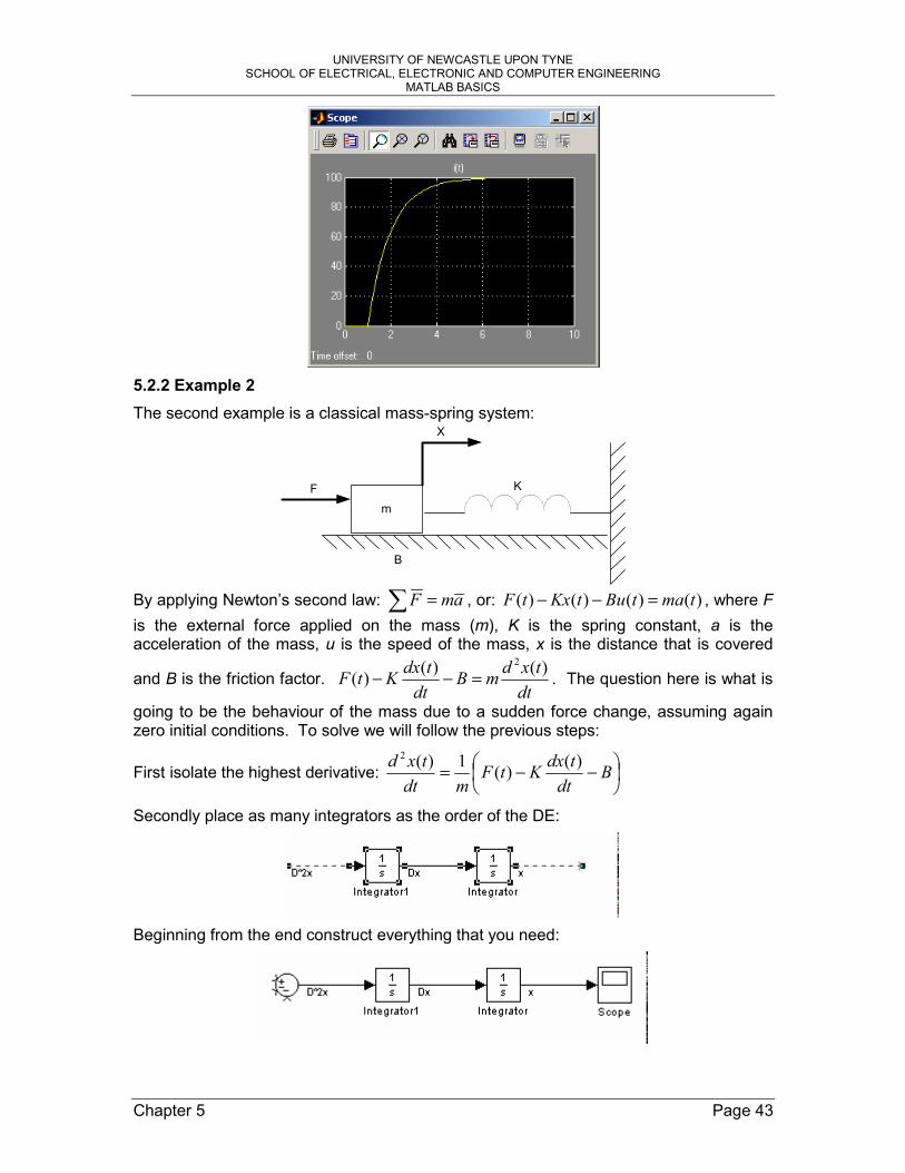
5.2.2 Example 2 The second example is a classical mass-spring system:
K
mF
X
B
By applying Newton’s second law: amF =∑ , or: )()()()( tmatButKxtF =−− , where F is the external force applied on the mass (m), K is the spring constant, a is the acceleration of the mass, u is the speed of the mass, x is the distance that is covered
and B is the friction factor. dttxdmB
dttdxKtF )()()(
2
=−− . The question here is what is
going to be the behaviour of the mass due to a sudden force change, assuming again zero initial conditions. To solve we will follow the previous steps:
First isolate the highest derivative:
−−= BdttdxKtF
mdttxd )()(1)(2
Secondly place as many integrators as the order of the DE:
Beginning from the end construct everything that you need:

UNIVERSITY OF NEWCASTLE UPON TYNE SCHOOL OF ELECTRICAL, ELECTRONIC AND COMPUTER ENGINEERING
MATLAB BASICS
Chapter 5 Page 44

UNIVERSITY OF NEWCASTLE UPON TYNE SCHOOL OF ELECTRICAL, ELECTRONIC AND COMPUTER ENGINEERING
MATLAB BASICS
Chapter 5 Page 45
5.2.3 Example 3 The pendulum shown has the following nonlinear DE:
0)sin(2 =++•••
aMgRabaMR
Its Simulink block is:
To find its response we must double click on the last integrator whose output is the angle a and set the initial conditions to 1.
5.2.4 Exercise
Solve the following nonlinear DE: ( ) 012 2 =−−+•••kxxxcxm . Take: m=1, c=0.1 k=1.
This is the Van der Pol equation and can correspond to a mass spring system with a variable friction coefficient.
R
a

UNIVERSITY OF NEWCASTLE UPON TYNE SCHOOL OF ELECTRICAL, ELECTRONIC AND COMPUTER ENGINEERING
MATLAB BASICS
Chapter 5 Page 46
These are two examples of Simulink design based on a previous Matlab version.
5.3 Second Order System Example
Simulation of the impulse and step response of a second-order continuous-time transfer function:
2
2 2( )2
n
n n
H ss s
ωζω ω
=+ +
, 1nω =
The following cases will be investigated: (a) Underdamped: 0 1ζ< < (b) Critically damped: 1ζ = (c) Overdamped: 1ζ >
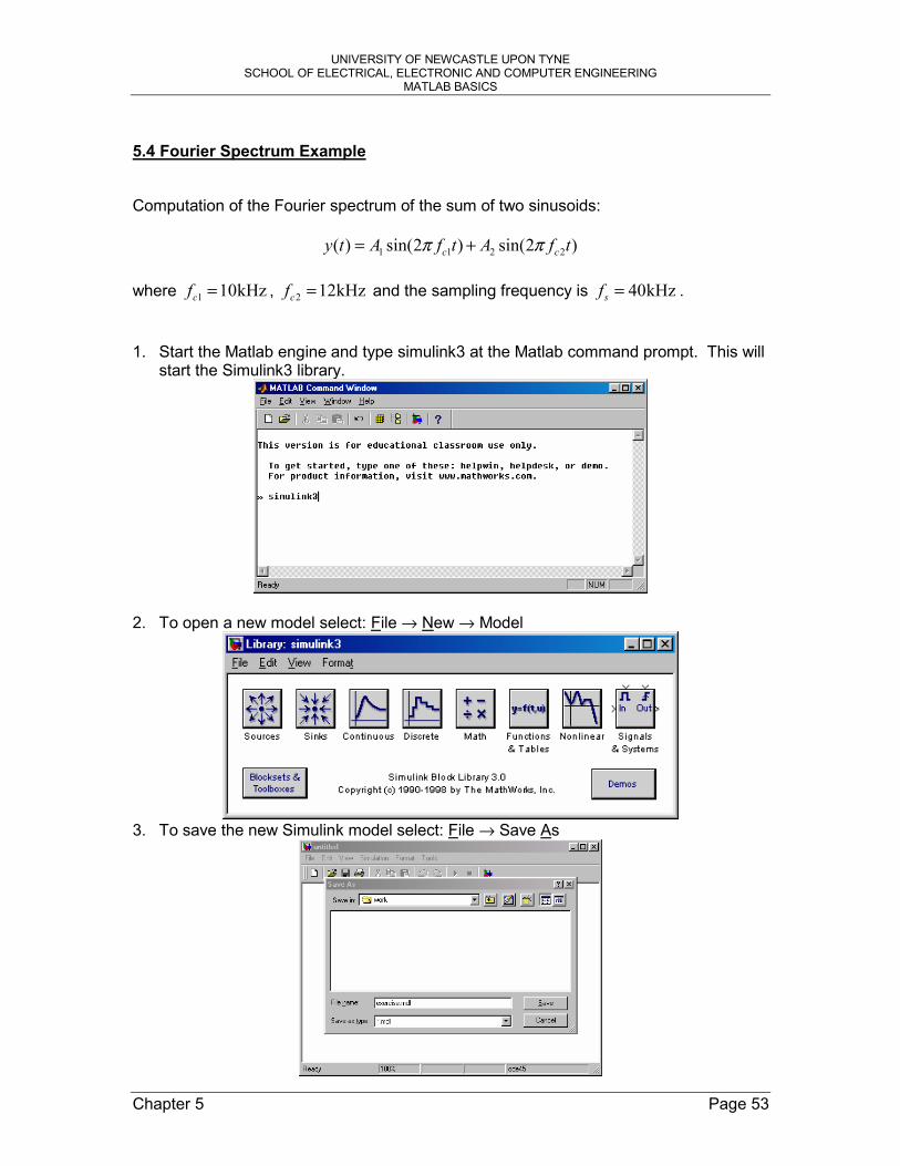
1. Start the Matlab engine and type simulink3 at the Matlab command prompt. This will start the Simulink3 library.

UNIVERSITY OF NEWCASTLE UPON TYNE SCHOOL OF ELECTRICAL, ELECTRONIC AND COMPUTER ENGINEERING
MATLAB BASICS
Chapter 5 Page 47
2. To open a new model select: File → New → Model
(The following window should appear.)
3. To save the new Simulink model select: File → Save As

UNIVERSITY OF NEWCASTLE UPON TYNE SCHOOL OF ELECTRICAL, ELECTRONIC AND COMPUTER ENGINEERING
MATLAB BASICS
Chapter 5 Page 48
4. Drag & drop two sine-wave blocks and a summation block from the Simulink3 libraries as illustrated below.

UNIVERSITY OF NEWCASTLE UPON TYNE SCHOOL OF ELECTRICAL, ELECTRONIC AND COMPUTER ENGINEERING
MATLAB BASICS
Chapter 5 Page 49
5. Double-click the step function block and insert the parameters as shown below.
6. Repeat for the transfer function block.
wn
Znω
ζ→
→
Right-click and drag the transfer function block to replicate it. Alternatively, you can use the following shortcuts for the same task: click on the transfer function block and Ctrl + C, Ctrl + V. 7. Double-click the scope block and insert the following parameters.
Replicate the scope block
UNIVERSITY OF NEWCASTLE UPON TYNE SCHOOL OF ELECTRICAL, ELECTRONIC AND COMPUTER ENGINEERING
MATLAB BASICS
Chapter 5 Page 50
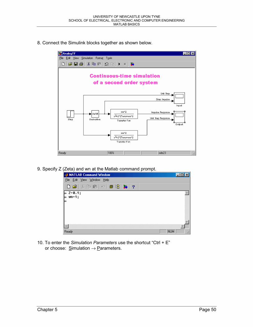
8. Connect the Simulink blocks together as shown below.
9. Specify Z (Zeta) and wn at the Matlab command prompt.
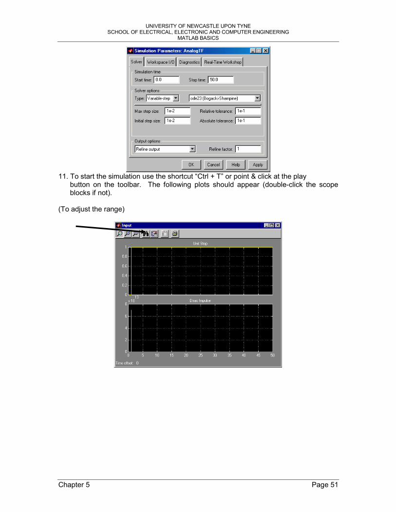
10. To enter the Simulation Parameters use the shortcut “Ctrl + E” or choose: Simulation → Parameters.
UNIVERSITY OF NEWCASTLE UPON TYNE SCHOOL OF ELECTRICAL, ELECTRONIC AND COMPUTER ENGINEERING
MATLAB BASICS
Chapter 5 Page 51
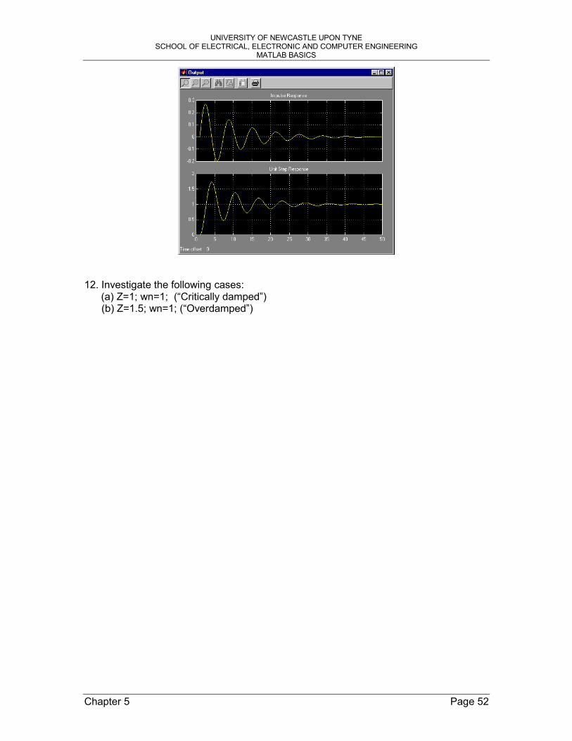
11. To start the simulation use the shortcut “Ctrl + T” or point & click at the play
button on the toolbar. The following plots should appear (double-click the scope blocks if not).
(To adjust the range)
UNIVERSITY OF NEWCASTLE UPON TYNE SCHOOL OF ELECTRICAL, ELECTRONIC AND COMPUTER ENGINEERING
MATLAB BASICS
Chapter 5 Page 52
12. Investigate the following cases: (a) Z=1; wn=1; (“Critically damped”) (b) Z=1.5; wn=1; (“Overdamped”)
UNIVERSITY OF NEWCASTLE UPON TYNE SCHOOL OF ELECTRICAL, ELECTRONIC AND COMPUTER ENGINEERING
MATLAB BASICS
Chapter 5 Page 53
5.4 Fourier Spectrum Example
Computation of the Fourier spectrum of the sum of two sinusoids:
1 1 2 2( ) sin(2 ) sin(2 )c cy t A f t A f tπ π= +
where 1 10kHzcf = , 2 12kHzcf = and the sampling frequency is 40kHzsf = . 1. Start the Matlab engine and type simulink3 at the Matlab command prompt. This will
start the Simulink3 library.
2. To open a new model select: File → New → Model
3. To save the new Simulink model select: File → Save As

UNIVERSITY OF NEWCASTLE UPON TYNE SCHOOL OF ELECTRICAL, ELECTRONIC AND COMPUTER ENGINEERING
MATLAB BASICS
Chapter 5 Page 54
4. Drag & drop two sine-wave blocks and a summation block from the Simulink3 libraries as illustrated below.

UNIVERSITY OF NEWCASTLE UPON TYNE SCHOOL OF ELECTRICAL, ELECTRONIC AND COMPUTER ENGINEERING
MATLAB BASICS
Chapter 5 Page 55
5. Open the DSP Library by typing dsplib at the command prompt.
6. Open the DSP Sinks library by double-clicking the corresponding icon.
7. Drag & drop the buffered FFT scope block.

UNIVERSITY OF NEWCASTLE UPON TYNE SCHOOL OF ELECTRICAL, ELECTRONIC AND COMPUTER ENGINEERING
MATLAB BASICS
Chapter 5 Page 56
8. Connect the Simulink blocks.
9. To enter the sine-wave block parameters double-click the corresponding icon. Recall: Amplitude * sin (2 * pi * Frequency * t + Phase)
where t = 0, Ts, 2*Ts, 3*Ts,…
10. Repeat for the block sine-wave1.
UNIVERSITY OF NEWCASTLE UPON TYNE SCHOOL OF ELECTRICAL, ELECTRONIC AND COMPUTER ENGINEERING
MATLAB BASICS
Chapter 5 Page 57
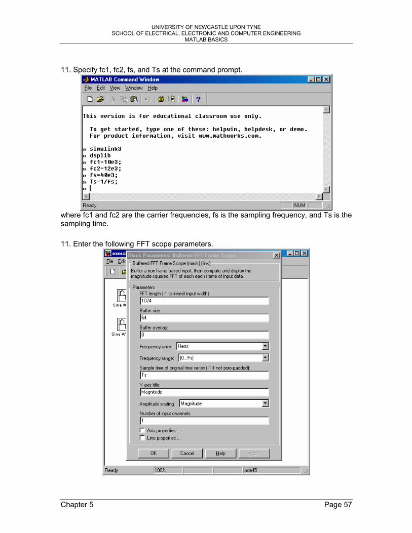
11. Specify fc1, fc2, fs, and Ts at the command prompt.
where fc1 and fc2 are the carrier frequencies, fs is the sampling frequency, and Ts is the sampling time. 11. Enter the following FFT scope parameters.

UNIVERSITY OF NEWCASTLE UPON TYNE SCHOOL OF ELECTRICAL, ELECTRONIC AND COMPUTER ENGINEERING
MATLAB BASICS
Chapter 5 Page 58
12. Finally, to enter the Simulation Parameters use the shortcut “Ctrl + E” or choose: Simulation → Parameters.
13. To start the simulation use the shortcut “Ctrl + T”
or point & click at the play button on the toolbar.
14. Once the simulation is running right click on the scope window and choose autoscale. The following plot should appear.
Explain the resulting spectral components by considering the following Fourier transform pair:
1 1sin(2 ) ( ) ( )2 2FT
c c cf t f f f fj jπ δ δ↔ − − +

UNIVERSITY OF NEWCASTLE UPON TYNE SCHOOL OF ELECTRICAL, ELECTRONIC AND COMPUTER ENGINEERING
MATLAB BASICS
Chapter 5 Page 59
15. Change the amplitude of the sine-wave1 to 0.5, save the changes, and re-run the simulation.
Explain the resulting spectrum. 16. Change fc2 to 25 kHz, save the changes, and re-run the simulation.
Explain the spectral component at 15 kHz. Determine the spectral components for fc2 = 35 kHz and 55 kHz (first without running the simulation). Now, verify your results by means of simulation. 17. Try the following frequencies for fc2: 20, 60, 80, 100 kHz.
Explain the resulting spectrum. Why is there is no spectral component at 20 kHz? 17. Double-click on sine-wave1 block and change the phase parameter to pi/2. Now
try the above frequencies again.

UNIVERSITY OF NEWCASTLE UPON TYNE SCHOOL OF ELECTRICAL, ELECTRONIC AND COMPUTER ENGINEERING
MATLAB BASICS
Chapter 5 Page 60
Explain the resulting spectrum. Why does the magnitude of the spectral component at 20 kHz equals those at 10 and 30 kHz? 18. Now, use fundamental blocks of the DSP library to design an FFT spectrum analyser
as illustrated below.
For the same set-up the FFT analyser should produce the same output as the Buffered FFT Frame scope. Describe the changes required to obtain a DFT spectrum analyser.