university of warwick institutional repository: · contents contents i declarations iii...

University of Warwick institutional repository: http://go.warwick.ac.uk/wrap

A Thesis Submitted for the Degree of PhD at the University of Warwick

http://go.warwick.ac.uk/wrap/62639

This thesis is made available online and is protected by original copyright.

Please scroll down to view the document itself.

Please refer to the repository record for this item for information to help you to cite it. Our policy information is available from the repository home page.

http://go.warwick.ac.uk/wrap

http://go.warwick.ac.uk/wrap/62639

Limit theorems leading to Bose-Einstein,

Maxwell-Boltzmann Statistics and Zipf-Mandelbrot

Law

by

Tomasz Michal Lapinski

Thesis

Submitted to the University of Warwick

for the degree of

Doctor of Philosophy

Department of Statistics

October 2013

Contents

Contents i

Declarations iii

Acknowledgments v

Abstract vii

List of Figures ix

Chapter 1 Introduction 1

1.1 Inspiration from the work of Prof. V.P. Maslov, Literature review . 2

1.2 Statistical Physics: Bose-Einstein and Maxwell-Boltzman statistics 13

1.2.1 Physical system under consideration, ideal mono-atomic gas

in the equilibrium . . . . . . . . . . . . . . . . . . . . . . . 13

1.2.2 Derivation of Bose-Einstein and Maxwell-Boltzmann statistics 16

1.3 Complexity Science: Zipf Law and other Power Laws . . . . . . . . 24

1.4 Thesis outline . . . . . . . . . . . . . . . . . . . . . . . . . . . . . . 28

Chapter 2 Limit theorems 31

2.1 Introduction . . . . . . . . . . . . . . . . . . . . . . . . . . . . . . . 31

2.2 Limit Theorem . . . . . . . . . . . . . . . . . . . . . . . . . . . . . 34

2.3 Fluctuation theorem, maximum in the interior of the domain . . . 44

2.4 Fluctuation theorem, maximum on the boundary of the domain . . 52

2.5 Related results . . . . . . . . . . . . . . . . . . . . . . . . . . . . . 57

Chapter 3 Entropy related results 68

3.1 Entropy approximation . . . . . . . . . . . . . . . . . . . . . . . . 69

i

3.2 Optimization . . . . . . . . . . . . . . . . . . . . . . . . . . . . . . 83

3.2.1 Optimization of the limit of the approximated entropy . . . 83

3.2.2 Optimization of the approximated entropy . . . . . . . . . . 89

3.2.3 Related results . . . . . . . . . . . . . . . . . . . . . . . . . 91

3.3 Related estimates . . . . . . . . . . . . . . . . . . . . . . . . . . . . 98

3.3.1 Estimates for the maximums . . . . . . . . . . . . . . . . . 99

3.3.2 Estimates for the first derivatives . . . . . . . . . . . . . . . 105

3.3.3 Estimates for the second derivatives . . . . . . . . . . . . . 108

3.4 Partition function approximation . . . . . . . . . . . . . . . . . . . 111

Chapter 4 Extended Laplace approximation 113

4.1 One-dimensional function with the maximum on the boundary of

the domain . . . . . . . . . . . . . . . . . . . . . . . . . . . . . . . 114

4.2 m-dimensional function with the maximum in the interior of the

domain . . . . . . . . . . . . . . . . . . . . . . . . . . . . . . . . . 119

4.3 m-dimensional function with the maximum on the boundary of the

domain . . . . . . . . . . . . . . . . . . . . . . . . . . . . . . . . . 125

Chapter 5 Conclusions, possible applications and future research 129

5.1 Conclusions . . . . . . . . . . . . . . . . . . . . . . . . . . . . . . . 129

5.1.1 Continuation of the work of Prof. V.P. Maslov . . . . . . . 130

5.1.2 Contribution to Statistical Physics . . . . . . . . . . . . . . 131

5.1.3 Contribution to Complexity Science . . . . . . . . . . . . . 132

5.1.4 Interdisciplinary contribution - unification of Statistical Physics

and Complexity Science . . . . . . . . . . . . . . . . . . . . 133

5.2 Possible application - Maxwell-Boltzmann, Bose-Einstein statistics

and Zipf Law as a description of state of economy . . . . . . . . . 133

5.3 Future research . . . . . . . . . . . . . . . . . . . . . . . . . . . . . 134

Appendix A Mathematical preliminaries 137

A.1 Analysis . . . . . . . . . . . . . . . . . . . . . . . . . . . . . . . . . 137

A.2 Asymptotic theory, approximations and related results . . . . . . . 142

A.3 Probability . . . . . . . . . . . . . . . . . . . . . . . . . . . . . . . 151

A.4 Theory of Optimization . . . . . . . . . . . . . . . . . . . . . . . . 152

Bibliography 155

ii

Declarations

I hereby declare that this thesis is the result of my own work and research, except

where otherwise indicated. This thesis has not been submitted for examination to

any institution other than the University of Warwick.

Signed:

Tomasz Lapinski

28th October 2013

iii

Acknowledgments

I would like to dedicate special thanks to my supervisor Prof. Vassili Kolokoltsov

for the ideas, patience and supervision during the time of my PhD. I would also

like to thank my personal tutor John Warren and other staff at the Department

for their support and the enjoyable times I have had.

For their support and faith in me I send special thanks to my parents and friends.

During the time of this PhD I have had a very nice and supportive

companionship and for that I thank my office mates and colleagues. I very much

appreciate tea time with Duy, lunch with Helen and parties and pleasant times

with other Warwick friends.

Tomasz Lapinski

28th October 2013

v

Abstract

In this thesis we develop the ideas introduced by V.P. Maslov in [9], [10] and

[11], the new limit theorem which leads to Bose-Einstein, Maxwell-Boltzmann

Statistics and Zipf-Mandelbrot Law. We independently constructed the proof for

the theorem, based on Statistical Mechanics methodology, but with precise and

rigorous estimates and rate of convergence. The proof involves approximation of

the considered entropy, the partition function and specific Laplace type integral

approximation which we had to develop specifically for this result. The proof

also involved several minor estimates and approximations that are included in

the work and the mathematical preliminaries which we used are attached in the

appendix. In addition, we provide a step by step introduction to the underlying

mathematical setting. Within the theorem we separated two cases of resulting

distribution, this separation was mentioned in [11] however it was not developed

further in that paper. The first case gives known distributions which are in the

thesis title. Additionally, we construct two new fluctuation theorems with proof

based on the proof of the main theorem. In terms of the application, we found

that developed theory can be applied in the field of Econophysics. Based on the

paper by F.Kusmartsev [16], we inferred that presented three distribution may

correspond to the state of the economy of particular countries. Unified underlying

framework might reflect the fact that these economies have one common structure.

vii

List of Figures

1.1 Zipf Law for the first volume of Leo Tolstoy’s ’War and Peace’ . . 11

1.2 Model fit of car brands prices on American market . . . . . . . . . 12

1.3 Japanese candles of the stock . . . . . . . . . . . . . . . . . . . . . 12

1.4 Diagram of evolution of Complexity Science . . . . . . . . . . . . . 26

1.5 Ranking of city sizes around the year 1920 . . . . . . . . . . . . . . 27

1.6 Illustration of Gutenberg-Richter law a) logarithmic plot of occured

earthquakes , b) corresponding places of occurrence . . . . . . . . . 27

1.7 Illustration of earthquakes worldwide since 1940 . . . . . . . . . . . 28

1.8 Plot of extinctions throughout the history of earth . . . . . . . . . 29

1.9 Power spectrum of traffic jam . . . . . . . . . . . . . . . . . . . . . 29

ix

1Introduction

The main purpose of this thesis is to present new mathematical results related

to Physics and indicate some possible applications within various scientific disci-

plines. As the title states, these new results are the limit theorems. The branch of

Mathematics which deals with limit theorems is Probability Theory, hence these

are probabilistic results. Further, as stated in the title, the outcomes of limit theo-

rems, Bose-Einstein and Maxwell-Boltzmann statistics, are common distributions

in the major field of Physics, Statistical Mechanics. The Zipf-Madlebort Law,

which is the third outcome of the theorems, is a power law widely occurring in

the Science of Complex Systems. Hence, to be more precise, this thesis is about a

new result of Probability Theory related to Statistical Mechanics and Complexity

Science.

In this introduction we provide an extensive background for the theorems.

We include a broad literature review of the existing ideas of where the theo-

rem originated from. We provide a short historical background of the fields and

branches in which the theorems have fundaments. What is more, we describe in

detail the particular results which are common and occur in this thesis. We also

include a depiction of their development on the historical timeline. The last part

of the introduction is an outline of the structure of the whole thesis.

The introduction chapter is structured into four sections. The first section

is about the origin of the idea of the theorems. It is mostly a review of several

papers by Prof. V.P. Maslov which seeded this idea and a short introduction of the

author. The next section is about Statistical Physics. We provide historical outline

of this field, we underline the significance of Thermodynamics in its development

and other important historical facts and scientific achievements. We include a

brief history of Bose-Einstain and Maxwell-Boltzmann statistics, together with

their derivations, and which are common to physicists. The third section concerns

Complexity Science. We begin with a little history of how this discipline evolved

1

over time. Then we explain the emergence of power laws, in particular the Zipf-

Mandelbrot Law. We will give the vast examples of power law systems to underline

its significance in the real world. In the last section, the full outline of the thesis

will be provided. We shortly describe the chapters which the thesis consist of and

include some interplay between these chapters too.

1.1 Inspiration from the work of Prof. V.P. Maslov,

Literature review

Viktor Pavlovich Maslov is a Professor at Lomonosov Moscow State University.

He is a specialist in the field of mathematical physics but his research spreads

over various branches of mathematical and natural sciences, particularly quantum

theory, asymptotic analysis, operator theory and nanotechnology.

He has gained recognition as a scientist who has a grasp in uncovering mathemat-

ics behind various phenomena from physics and other natural sciences.

An example here can be his development of the first formal mathematical de-

scription of a nanostructure, which resulted in the introducing of an object called

Lagrangian submanifold. V.P. Maslov is also known for the introduction of a

Maslov index.

A peer-review journal Mathematical Notes, which is a translation of Matematich-

eskie Zametki, is the main mathematical journal of the Russian Academy of Sci-

ence. Prof. V.P. Maslov is its editor-in-chief and there he publishes some of his

findings. Among many branches of mathematics, one can find works published

in number theory, functional analysis, topology, probability, operator and group

theory, asymptotic and approximation methods spectral theory and other fields.

Most of the publications which are fundamental for our work were released in this

journal. For more information about V.P.Maslov see [6].

Here we will review four of his papers. The first paper ’Nonlinear averaging

axioms in financial mathematics and stock price dynamics’, provided some back-

ground to the nonlinear averages introduced by Maslov in economics and their

connection to Statistical Mechanics. Then, in ’Nonlinear averaging in Economics’

an extension of this nonlinear average to a more general context than economics is

provided and a more explicit connection with statistical physics is given. The con-

vergence of nonlinear average to Bose-Einstein statistics is also introduced. These

findings are placed in the form of the limit theorem with drafts of the proof.

2

Finally in the third paper ’On a General Theorem of Set theory leading to the

Gibbs, Bose-Einstain and Pareto Distributions as well as to the Zipf-Mandelbrot

Law for the Stock Market’ the nonlinear average is further generalised. This gen-

eralisation is of a mathematical nature. Instead of convergence to one statistics,

i.e. Bose-Einstein, we have convergence to three, two others are Gibbs type and

Pareto distribution. Obtaining one of three averages is determined by choice of

some parameter. Our work is an extension and development of the findings of

this paper. In the last paper of V.P.Maslov that we review, ’On Zipf’s Law and

Rank Distributions in Linguistics and Semiotics’, he first underlines the signifi-

cance of Zipf Law, recalls its origins and then introduces a new framework for how

to model various systems with Zipf related laws. For us this paper was signifi-

cant as it showed the generality of Zipf Law and related distributions in nature.

Given that in previous paper the mathematical derivation of Zipf Law was given,

exploring those various system modelled by Zipf Law was even more inspiring.

Review of Nonlinear averaging aximos in financial mathematics and

stock price dynamics

First we consider the paper ’Nonlinear averaging axioms in financial mathemat-

ics and stock price dynamics’ [10]. The author begins with an introduction to

the certain type of nonlinear average and supports the fact of nonlinearity with

two examples. In calculating the individual ’natural’ capital, one has to consider

many factors. One common way is to consider a credit which can be given to

particular individuals and this depends on many factors. These factors can be

regular income, employment status, age, number of dependencies , credit history

and others. Obviously, the person’s capital is not a linear dependence of possessed

money and income.

Another example of nonlinear averaging occuring naturally is the stockholder’s

ability to influence the company, i.e. 51 percent of stock gives the right to decide

50 not. We see that the percentage of stocks possessed is not a linear dependence

with ability to influence the company.

Further, the axioms of nonlinear averaging are introduced. He considers the

3

avarage of the form

y = f−1

(∑i

αif(xi)

),

xi =

G∑j=1

λjNj ,

where f is come convex function, αi are weight factors and y is a nonlinear average

of the incomes xi.

Additionally the income xi is composed of the incomes from G assets, each corre-

sponding to outcomes λj and quantity of money Nj . We also have that∑G

j=1Nj =

N and N is the total amount of money invested.

Furthermore the ’degenerations’ are included, i.e. there are G1 same outcome λ1

over which capital is redistributed and also G2 of λ2, and so on. Hence xi are

equal

xi = λ1

G1∑j=1

Nj + λ2

G∑j=G1+1

Nj ,

for two different outcomes λ1, λ2 only.

The axioms from the paper are the following

• Axiom 1 states that when there is only one income xi then average simply

becomes this income.

• Axiom 2 restricts that the coefficients αi are independent of λj .

• Axiom 3 defines that two notes of money are indistinguishable.

• Axiom 4 states if we add some value ω to all λj then income xi will increase

by the same value Nω.

The author applies these axioms to calculate the function f and weights αi, this

leads to the ’financial averaging formula’ for two outcomes λ1 and λ2

y =1

βlog

((G− 1)!N !

(N +G− 1)!

N∑N1=0

(G1 +N1 − 1)!

(G1 − 1)!N1!

(G2 +N2 − 1)!

(G2 − 1)!N2!exp

(β(λ1N1+λ2N2)

)),

(1.1)

where

αi = αN1 =(G− 1)!N !

(N +G− 1)!

(G1 +N1 − 1)!

(G1 − 1)!N1!

(G2 +N2 − 1)!

(G2 − 1)!N2!

4

and N2 = N −N1, G2 = G−G1.

It turns out that Axiom 3 about the indistinguishability of notes corresponds

to assumptions about bosons in the Bose-Einstein statistics and the coefficients

αi correspond to a number of possible redistributions of N1 boson particles over

energy level with G1 degenerations and N2 bosons over G2 degenerations.

What is more, the exponent function f and constant β correspond to the Gibbs

factor.

As an example of such averaging, Prof. Maslov considers two groups of financial

institutions. The first group gives return λ1 and there are G1 institutions in this

group. The second provides outcome λ2 and there are G2 of them. Additionally,

money deposited in the first group is subject to taxation proportional to the square

of money deposited, while depositors of the second group get a subsidy which is

also proportional to the square of money put in the second group institutions.

Hence the income xi is equal

xi = λ1N1 + λ2N2 −V1N

21

2N+V2N

22

2N,

where V1, V2 are constants corresponding to taxation and subsidy, and N1 is money

put in the first group and N2 into second. The value of N2 can be expressed via

N1, i.e. N2 = N−N1, then the ’financial averaging formula’ (1.1) can be expressed

as

y =1

βln

( N∑N1=0

exp(F (N1))

)(1.2)

where F (N1) has from

F (N1) =β(λ1N1 + λ2(N −N1)− V1N21

2N+V2(N −N1)2

2N)− ln

(n− 1)!N !

(N + n− 1)!+ ln

(G1 +N1 − 1)!

(G1 − 1)!N1!+

+ ln(G−G1 +N −N1 − 1)!

(G−G1 − 1)!(N −N1)!.

Further, the author approximates F (N1) ≈ Nf(x) where x = N1N as N →∞ with

assumptions

limN→∞

G1

N= g1 > 0,

limN→∞

G2

N= g2 > 0,

5

and obtains

y =1

βln

( N∑Nx=0

exp(Nf(x))

),

Next the author uses method similar to Laplace approximation to find values of

x which is a biggest weight in the average, i.e. maximum of f(x) for large values

of N .

The main conclusion of the paper is that finding several points of such maximum

depend on the values of the parameter β.

Review of Nonlinear averaging in Economics

The second paper of V.P.Maslov we review is ’Nonlinear averaging in Economics’,

[9]. Here the author recalls the four Kolmogorov nonlinear averaging axioms. The

class of functions which are obtained as a result of those axioms contains the

function which was specified in nonlinear financial averaging from the previous

paper. Then the fifth axiom is added and as a consequence, the class function is

restricted to a function exactly the same as the one which comes from the Axioms

of averaging in economy.

Further, the nonlinear average is introduced for the general case. There are n

different prices and to each one corresponds number of financial instrument Gi

having the price λi. The number of different possibilities the buyer can spend Ni

amount of money in Gi number of instruments is given by the formula

γi(Ni) =(Ni +Gi − 1)!

Ni!(Gi − 1)!

Then N = (N1, N2, . . . , Nm) is a set corresponding to a particular allocation of

money N , where∑n

i=1Ni = N . The number of different possibilities how such

allocation can be done is equal

γ(N ) =

n∏i=1

γi(Ni) =

n∏i=1

(Ni +Gi − 1)!

Ni!(Gi − 1)!.

The expenditure for some particular allocation N is given by

x(N ) =

n∑i

λiNi,

6

and finally the nonlinear averaging for the general case is specified as

y = − 1

βln

(N !(G− 1)!

(N +G− 1)!

∑N

γ(N ) exp(−βx(N ))

).

where the sum is over all possible sets N denoted as N such that∑n

i=1Ni = N

and also∑n

i=1Gi = G.

Bought assets are additionally put into m groups with the index α, where the

particular group has assets starting from the index iα and ending on jα, hence

iα ≤ jα, iα+1 = jα + 1, α = 1, . . . ,m, i1 = 1, jm = n,

then we have also following

Gα =

jα∑i=iα

gi, Nα =

jα∑i=iα

ki.

As the author is interested in the behaviour of the average in the limit as N →∞he makes assumptions on how the number of instruments increase as available

money increases, i.e.

limN→∞

G

N= g,

limN→∞

GαN

=gα > 0,m∑α=1

gα = g,

limN→∞

Nα

N=nα > 0,

∑nα = 1.

Further, he claims that the average number of money put in certain groups is

equal to

Nα(β,N) =

jα∑i=iα

giexp(β(λi + ν))− 1

which corresponds to the number of particles on energy levels with energies λi and

the number of level degenerations gi in Bose-Einstein statistics.

The parameter ν is specified by the equation

N =

n∑i=1

Giexp(β(λi + ν))− 1

.

7

and he introduces function Γ(β,N)

Γ(β,N) =∑N

γ(N ) exp(−βx(N )) (1.3)

Now we recall the main result of the paper, the limit theorem

Theorem 1. Let ∆ = aN3/4+δ where a and δ < 1/3 are some positive constants.

Then for any ε > 0, the following relation holds as N →∞

1

Γ(β,N)

∑∑mα=1(Nα(N )−Nα(β,N))2≥∆

γ(N ) exp(−βx(N )) =

=O

(exp

((1− ε)a2N1/2+2δ

2gd

)),

where the summation is over the collection of the sets N such that condition∑mα=1(Nα(N )−Nα(β,N))2 ≥ ∆ is satisfied and d is defined as

d =exp(−β(λ1 + ν))

(exp(−β(λ1 + ν)− 1)2, for β < 0,

d =exp(−β(λn + ν))

(exp(−β(λn + ν)− 1)2, for β > 0.

This can be put in the context of finance as the contribution to average expenditure

which is the square difference from Nα(β,N) by more than value O(N3/4+δ) is of

exponentially small value for a sufficient large N .

The author provides draft of the proof of that theorem. It is a mixture of

some methods from statistical physics and asymptotic analysis.

Review of On a General Theorem of Set theory leading to the Gibbs,

Bose-Einstain and Pareto Distributions as well as to the Zipf-Mandelbrot

Law for the Stock Market

Next, we review the paper ’On a General Theorem of Set theory leading to the

Gibbs, Bose-Einstein and Pareto Distributions as well as to the Zipf-Mandelbrot

Law for the Stock Market’, [11]. The nonlinear average here is put in the broader

context of sets. This time, instead of average expenditure we have a set of integers

N1, N2, . . . , Nn, which are nonlinear average integers in the collection of the set

8

N such that N = (N1, N2, . . . , Nm) and∑n

i=1Ni = N for some integrer N .

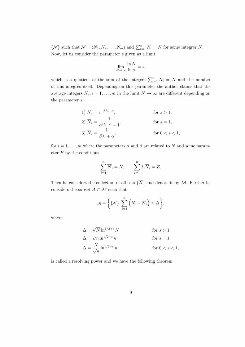
Now, let us consider the parameter s given as a limit

limN→∞

lnN

lnn= s,

which is a quotient of the sum of the integers∑n

i=1Ni = N and the number

of this integres itself. Depending on this parameter the author claims that the

average integers N i, i = 1, . . . ,m in the limit N → ∞ are different depending on

the parameter s

1) N i = e−βλi−α, for s > 1,

2) N i =1

eβλi+α − 1, for s = 1,

3) N i =1

βλi + α, for 0 < s < 1,

for i = 1, . . . ,m where the parameters α and β are related to N and some param-

eter E by the conditions

n∑i=1

N i = N,n∑i=1

λiN i = E.

Then he considers the collection of all sets N and denote it by M. Further he

considers the subset A ⊂M such that

A =

N,

n∑i=1

(Ni −N i

)≤ ∆

,

where

∆ =√N ln1/2+εN for s > 1,

∆ =√n ln1/2+ε n for s = 1,

∆ =N√n

ln1/2+ε n for 0 < s < 1,

is called a resolving power and we have the following theorem

9

Theorem 2. As N →∞ the following inequality holds

Nm(M\A)

Nm(M)≤ C

n+C

N, (1.4)

where C is some constant and Nm denotes the number of elements in the sets

M\A and M.

In other words, the theorem states that the contribution of the sets that

differs by more than delta from the given average set is decreasing as N →∞ as

1/N and 1/n.

Note, that th eabove theorem is similar to one from the previous paper, but there

the author considered only the second case of the average and the contribution

was exponentially small instead of 1/N and 1/n.

Prof. Malsov includes the draft of the proof of that theorem in this paper. He

uses there methods form analysis, asymptotic theory and statistical mechanics.

Throughout the paper the author connects the averages of the theorem with known

distributions. The first one relates to Gibbs type distribution, second is Bose-

Einstein statistics and the last one Pareto Distribution or Zipf-Mandlebrot Law.

On Zipf’s Law and Rank Distributions in Linguistics and Semiotics

The last paper which we review is ’On Zipf’s Law and Rank Distributions in Lin-

guistics and Semiotics’ [12]. In the beginning of this paper, the author introduces

Zipf’s Law. Taking a particular book, if one counts the occurring words in the

text, takes the frequencies for occurrence of each one and orders them in descend-

ing order then one will get the relation which will be close to Zipf Law. The

distance from the exact Zipf Law will vary from text to text, but for some it will

be exactly Zipf.

Some mathematicians and linguists saw, through computing and the development

of ’frequency dictionaries’ the possibility of creating an algorithm to distinguish

authorship.

However, V.P.Maslov is of the opinion that this situation with the frequency of

words is not that simple. He claims that the factual frequency of particular words

is actually higher than what one can count. One of the reasons is writing style,

some words are omitted, some replaced, some are substituted as certain styles by

default require that. Sometimes it may be because of shortcuts used in the style or

10

Figure 1.1: Zipf Law for the first volume of Leo Tolstoy’s ’War and Peace’

meaning behind certain phrases, which might be much bigger than crude words.

For a word Prof. Maslov defines this virtual frequency as

ωi = ωi(1 + αωγi ),

where α and γ are some parameters supposedly common to one text.

The main concept introduced in this paper is to extend the use of frequency dic-

tionaries from just text to a more general context, which would be a sign system.

Signs are of the interest of the discipline known as semiotics. In this general con-

text, distinct words occurring in the book is a sign, its frequency is this signs

cardinality and corresponding virtual frequency, virtual cardinality. The author

gives various examples of the sign system, a book in the library with a given title,

where the book database is a sign dictionary. Then the book requested in the

database is a real cardinality, but if one adds book usages by colleagues, relatives

this would be a virtual cardinality. Another example of sign could be a city. The

number of people living in the city, the number from the census is a real cardi-

nality but the number of people currently staying in the city, tourists, visitors of

family, business visitors etc. is a virtual cardinality.

The example explored in more detail by the author is the prices of car brands,

where the car brand is a sign and the car price is a cardinality. Then the virtual

cardinality includes, with the exception of the original car price, many other ex-

penses like insurance, gas, services and taxes.

11

Figure 1.2: Model fit of car brands prices on American market

The next example is Japanese candles, i.e. a day to day changes of the asset

prices, in the given example of some stock. The signs are the Japanese candles of

particular size and the real frequency their amount. The virtual cardinality can

correspond to the deal outside the stock exchange, by brokers themselves or other

networks.

Figure 1.3: Japanese candles of the stock

12

1.2 Statistical Physics: Bose-Einstein and Maxwell-

Boltzman statistics

This introduction is a compilation of relevant information from two books [5] and

[17].

Statistical mechanics, in general, is about the systems of very many par-

ticles. Such system can be studied from two points of view: microscopic, “small

scale”, which is roughly the size of single atom or molecule, usually of the order

10A and macroscopic, “large scale”, where system is visible in the ordinary sense

and it is of a size greater than 1 micron.

In the beginning, the “physical”homogeneous systems, such as liquids,

gases or solids, have been investigated only from the macroscopic point of view, as

the atomic nature of matter has not yet been well understood. Such description is

based on the quantities which describe system as whole, macroscopic quantities.

These quantities are related by the number of laws and together form a physics

branch called ‘thermodynamics”. This theory was developed in consistent form

by Clausius and Lord Kelvin in around 1850, and further extended by J.W. Gibbs

in around 1877.

Significant progress in the understanding of matter on the microscopic level

in the first half of the last century resulted in the development of quantum me-

chanics. Such development gave us the possibility to fully describe particles and

the interaction between them on the microscopic scale.

Two theories, thermodynamics and quantum mechanics opened the way to

form the theory which relates micro with macroscopic level. Statistical mechanics

has emerged from their unification. It yields all the laws of thermodynamics plus a

large number of relations connecting macroscopic quantities with the microscopic

parameters.

1.2.1 Physical system under consideration, ideal mono-atomic gas

in the equilibrium

Statistical mechanics is a broad field of physics, in the sense that it yields the

results for the distinct systems consisting of variety of molecules in various states.

However, one of the most common studied “class”of systems are the so-called ideal

gases. Note that for ideal gases the type of molecules can vary, this can be mono or

13

multi-atomic particles, bosons, fermions, helium, etc. Obviously this implies dif-

ferences in the obtained results. Considered systems can “change significantly”in

time, be time-dependent, i.e. non-equilibrium, or remain “stable”, be in equilib-

rium. There is a different approach to obtaining results for systems which are

in equilibrium and those which are non-equilibrium. Moreover, system state can

vary, which can be measured by the macroscopic and microscopic quantities. De-

pending on the state of the system we might use classical or quantum mechanics

to perform calculations. We will focus our attention on the model of ideal gas of

single atom in equilibrium. Next, we will explain the above assumptions in details.

The state of the system can be described by the macro and microscopic

quantities. For the gas the quantities which describe it as whole , i.e. macroscop-

ically, are:

• Volume V ,

• Energy E,

• Number of particles N ,

• Entropy S = k log Ω where Ω are systems accessible states and k is called

Boltzmann constant,

• Temperature T , which represents the relative change energy when we change

the entropy of system,

T =∂E

∂S.

The microscopic quantities are those which specify the states of single particles.

In case of the ideal gas those are the vectors of the position ri and momentum

pi, for i-th particle. Note that several other microscopic quantities can be derived

from those basic ones, for example speed. The number of particles which have

certain speed in system is also of microscopic quantity. To obtain such a quantity

one would require the information about all particles momentum.

Generally, gases behave as an ideal gas only under certain conditions. Phys-

ically, this situation occurs when the concentration of the molecules is sufficiently

small. However, speaking more rigorously, the potential energy, interactions, be-

tween particles have to be of negligible size. The following example illustrates this

situation.

14

Let us consider the gas of the N molecules confined in the container of the volume

V . The total energy of this system can be written as:

E = K + U + Eint,

where K denotes the kinetic energy of the molecules. If the momentum of i-th

molecule is given by the vector pi then K is equal to:

K(p1, p2, . . . , pN ) =1

2m

N∑i=1

p2i ,

where m is the mass of the single molecule. The quantity U = U(r1, r2, . . . , rN )

represents the potential energy of the mutual interaction of the particles and de-

pends on the centre-of-mass positions of the molecules ri. The term Eint is energy

of the intermolecular interaction, which for the mono atomic gases Eint = 0. We

call a gas an ideal if the potential energy of the interactions is negligibly small, i.e.

U ≈ 0. This usually can be achieved by increasing average distance between the

molecules so that the collisions are relatively rare. Obviously, this can be achieved

by, for example, decreasing the concentration of molecules N/V .

When we consider all possible configurations, i.e. microscopic states, as

separate systems, those instances form so-called statistical ensemble. The aim

of defining ensemble is to represent the probability of some systems while their

macroscopic parameters have certain values. This implies that only the fraction

of systems in ensemble will have this parameter of that specified value. We as-

sume that, while system is in equilibrium, all configurations occur with the same

probability, i.e. there is nothing special in any configuration to distinguish its

occurrence. This is known in statistical mechanics as basic statistical postulate.

We consider only the case of system in equilibrium, therefore this postulate will

be valid.

It is important to mention that, on the microscopic level the system is

governed by the laws of quantum mechanics. However, under some special cir-

cumstances for the large number of cases it obeys the laws of classical mechanics.

The simplification to classical description has some significant consequences in

computations. The essence of difference between classical and quantum descrip-

tion lies in the particles distinguishability. In other words, the number of systems

in ensemble can be altered due to the distinguishability of particles. For exam-

15

ple, if we interchange two particles and such change will result in obtaining two

different states, then we deal with distinguishable particles. This occurs only in

classical mechanics approximation. In quantum case the particles are considered

as identical and therefore indistinguishable. Moreover, due to quantum mechani-

cal results, we have two types of the identical particles: bosons and fermions. The

difference between them is in the restriction of number of the particles which can

have single energy value, i.e. occur on a single energy level. For fermions, only

one particle in a single state is allowed, while there is no restriction for bosons.

The difference is of significance while counting the number of constrained systems

accessible states. Technically we can check whether we should use the classical ap-

proach. This can be done by measuring some macroscopic quantities and checking

if the following condition holds

(V

N

) 13

h√3mkT

.

We can infer if we can use classical mechanics when the concentration of molecules

N/V is relatively small, temperature T and mass of molecule m are sufficiently

high.

1.2.2 Derivation of Bose-Einstein and Maxwell-Boltzmann statis-

tics

Both, Maxwell-Boltzmann and Bose-Einstein statistics give answers to the follow-

ing question: how particles are distributed over the spectrum of available energies

in the system, on average. Corresponding to our general overview of statistical

mechanics, having the values of some macroscopic quantities, measurement, in

our case fixed energy and the number of particles, we draw conclusions about

system on the microscopic level. The difference between two statistics is in the

distinguishability of particles, i.e. if we interchange two particles on two levels for

Maxwell-Boltzmann this will count as two micro states but for Bose-Einstein this

will be the same state, as essentially the number of particles on the energy levels

didn’t change.

In the literature there are two ways of deriving those statistics, the method

of averages which is based on the grand canonical ensemble and the second, based

16

on the entropy maximization, the method of most probable values.

Method of averages

The name of this method is related to the final result which is the average number

of particles in strict sense. The general formula for the average number of particles

N i having the energy εi

N i =

∑r

Ni,rΩ(Er, Nr)∑r

Ω(Er, Nr)=∑r

NiPr(Er, Nr),

where summation is over all distinguishable states r for all energy Er and number

of particles Nr

m∑i=1

Ni = N,

m∑i=1

εiNi = E,

and Ω(Er, Nr) is the number of accessible states for given Er and Nr. Each state

r corresponds to the particular vector of number of particles (N1, N2, . . . , Nm).

Next step is to approximate the probability Pr(Er, Nr). However, to do

that we first have to introduce the concept of reservoir.

Let us consider the situation when our system, denoted by A, is in contact with

hypothetical heat and particle reservoir A′. Both systems A + A′ = A(o) are

isolated, i.e. do not exchange heat or particles with outside, only between each

other. The total energy and particles are given by:

E + E′ = E(o) = constant,

N +N ′ = N (o) = constant,

where N,E are the particles and energy of our considered system, while E′ and

N ′ are of the reservoir. The system A′ is called reservoir because we assume that

its energy and the total number of particles change insignificantly after contact

with the considered system A, i.e. A′ is much bigger than A. Which also means

17

that E(o) Er and N (o) Nr and we have the approximation

∂2Ω′

∂E′2Er

∂Ω′

∂E′(1.5)

Then the probability Pr(Er, Nr) can be well approximated by considering

the combined system A(o) instead of just A. Let Ω′(E′, N ′) denote the number of

states accessible, i.e. entropy, of the reservoir A′ while A is in one of the definite

states r with Nr particles and energy Er. For that case the number of accessible

states for the combined system A(o) is just a number of states accessible for the

reservoir S′(E(o) − Er, N (o) −Nr) while the total amount of states accessible for

A(o) is Ω(o)(E(o), N (o)). The “starting”idea of the method is the equivalence of

probability between finding A in state r and finding A(o) in fraction of states that

A is in r and A′ is one of the S′(E(o) − Er, N (o) − Nr). It can be expressed in

formula:

Pr(Er, Nr) =Ω′(E(o) − Er, N (o) −Nr)

Ω(o)(E(o), N (o)).

We simplify the above formula by “extracting ”the dependency of Er and Nr from

S′. The procedure is following. We first represent S′ in terms of Taylor expansion

ln Ω′(E(o) − Er, N (o) −Nr) = ln Ω′(E(o), N (o))−[∂ ln Ω′

∂E′

]E′=E(o)

Er−

−[∂ ln Ω′

∂N ′

]N ′=N(o)

Nr + . . . ,

where higher terms are neglected due to conditions (1.5).

The appearing derivatives are denoted

λ =

[∂ lnS′

∂E′

]E′=E(o)

, ν =

[∂ lnS′

∂N ′

]N ′=N(o)

.

Then we exponentiate both sides

Ω′(E0 − Er, N0 −Nr) ≈ Ω′(E0, N0)e−λEr−νNr ,

and our probability is given by

Pr(Er, Nr) =Ω′(E(o), N (o))

Ω(o)(E(o), N (o))e−λEr−νNr .

18

Such class of probability distributions is called “grand canonical”distribution. The

first part of the expression on the right side is independent of the particular state r

and can be calculated from the normalization condition∑

r Pr = 1 and eventually

we have

Pr(Er, Nr) =e−λEr−νNr∑r

e−λEr−νNr.

Now, going back to our microscopic quantity - the average number of particles on

some energy level is given by the expression

N i =

∑r

Nie−λEr−νNr

∑r

e−λEr−νNr= − 1

λZ∂Z∂εi

, (1.6)

where two constant λ and ν are unknown and Z is called grand partition function

and is given by

Z =∑r

e−λEr−νNr .

The grand partition function is altered for Maxwell-Boltzmann statistics

and we have to add Gibbs correction factor to the exponent. Further we consider

the “degeneration”of the energy level. For each Ni particles on the level with

energy εi we can additionally redistribute them on the over the Gi sub-levels.

Physically, this corresponds to the fact that some energy levels in the system are

very close to one another and that is why they can be grouped as one. Due to

this degenerations, the grand partition function is altered for both statistics and

we provide the details separately for each statistics.

1. Maxwell-Boltzmann statistics

Here the additional factor for the grand partition factor is due to the distin-

guishability of particles and level degeneration and is given by

wM.B. =

m∏i=1

GNiiNi!

,

Hence the grand partition function is

ZM.B. =∑r

m∏i=1

GNiiNi!

e−λEr−νNr .

19

Next we transform it

∑r

m∏i=1

GNiiNi!

e−λEr−νNr =∞∑N=0

∑N1+N2+...+Nm=N

1

N !

N !

N1!N2! . . . Nm!

m∏i=1

(Gie

−λεi−ν)Ni

,

and using the multinomial theorem

(x1 + x2 + . . .+ xm)N =∑

N1+N2+...+Nm=N

N !m∏i=1

xNiiNi!

we get

∞∑N=0

∑N1+N2+...+Nm=N

1

N !

N !

N1!N2! . . . Nm!

m∏i=1

(Gie

−λεi−ν)Ni

=

∞∑N=0

1

N !

( m∑i=1

Gie−λεi−ν

)N,

where the outcome expression is a series representation of the exponent,

hence the grand partiton function for Maxwell-Boltzmann statistics is

ZM.B. = exp

( m∑i=1

Gie−λεi−ν

),

and we calculate the statistics itself from formula (1.6)

N i = Gie−λεi−ν .

Regarding the parameters λ and ν, for system with sufficiently large num-

bers of particles, the number of accessible states 1/∑

r e−λEr−νNr is rapidly

increasing function of E′ and N ′, on the other hand e−λEr−νNr is rapidly de-

creasing. In that situation the function e−λEr−νNr/∑

r e−λEr−νNr which is

our probability (1.2.2), experience very sharp maximum for some unknown

values λ and ν. This sharp peak occurs for the related values Er = E and

Nr = N . For other values Er and Nr the probabilities Pr(Er, Nr) ≈ 0. We

determine λ and ν by fixing quantities E and N obtained, possibly, by some

macroscopic measurement. The probability of finding system in E and N

is incomparably higher as for those values there was a sharp peak. Hence

we can assume that E and N are also average values, namely E = E and

20

N = N . Then we can calculate the parameters from the two equations

E =

m∑i=1

εiGie−λεi−ν ,

N =

m∑i=1

Gie−λεi−ν .

2. Bose-Einstein statistics

In this case alteration of grand partition function is due to the sublevels Gi.

We can express it in terms of combinatoric formula. A number of possibilities

of redistributing N1 indistinguishable particles over Gi sublevels is given

wB.E. =m∏i=1

(Ni +Gi − 1)!

Ni!(Gi − 1)!, (1.7)

and then

ZB.E. =

m∏i=1

(Ni +Gi − 1)!

Ni!(Gi − 1)!e−λEr−νNr ,

which can be simplified by using generalised geometric series formula

1

(1− x)s=∞∑n=0

(n+ s− 1

n

)xn.

hence we have

ZB.E. =

( ∞∑N1=0

(N1 +G1 − 1)!

N1!(G1 − 1)!e−(λε1+ν)N1

)( ∞∑N2=0

(N2 +G2 − 1)!

N2!(G2 − 1)!e−(λε2+ν)N2

). . . =

=

(1

1− e−λε1−ν

)G1(

1

1− e−λε2−ν

)G2

. . . =m∏i=1

(1

1− e−λεs−ν

)Gi,

and from (1.6) we get the Bose-Einstein statistics

N i =Gi

eλεi+ν − 1.

Here, similar to the situation for the Maxwell-Boltzmann statistics, we cal-

21

culate the statistics from the two equations

E =

m∑i=1

εiGi

eλεi+ν − 1,

N =

m∑i=1

Gieλεi+ν − 1

.

Method of most probable values

In this method we consider explicit function of number of accessible micro states

in the system, the entropy, and we find the most probable micro state and assume

this is the average state. We are given constraint for the number of particles and

energy

m∑i=1

Ni = N, (1.8)

m∑i=1

εiNi = E.

The number of accessible states to the system is

Ω(N,E) =∑Ni

W (Ni),

where sum Ni is sum over all possible vectors (N1, N2, . . . , Nm) that conform

to the conditions (1.8) and W (Ni) is a number of possible distribution corre-

sponding to given vector of Ni’s. Here we also consider the case when each i− thlevel has Gi sublevels.

1. Maxwell-Boltzmann statistics

In the case, due to distinguishability of particles, the W (Ni) is given by

WM.B.(Ni) =m∏i=1

(Gi)Ni

Ni!.

22

Then the systems entorpy is equal

S(N,E) = k ln Ω(N,E) = k ln

(∑Ni

m∏i=1

(Gi)Ni

Ni!

)

Now, we find the vector (N∗1 , N∗2 , . . . , N

∗m) in the sum for which the entropy

is largest and value for this vector will be much larger than for others in the

thermodynamical limit, hence we have approximation

S(N,E) ≈ k ln

( m∏i=1

(Gi)N∗i

N∗i !

), N →∞.

We find this vector by finding the maximum of the entropy using the La-

grange multipliers method. However, first we approximate the logarithm

with known Stirling formula for factorials lnN ! = N lnN − N , then the

entropy is

S(N,E) ≈m∑i=1

N∗i lnG(i)

N∗i.

Then the equation for maximum value is given by

∂

∂Ni

m∑i=1

[Ni ln

G(i)

Ni− λ

( m∑i=1

εiNi − E)− ν( m∑i=1

Ni −N)]

Ni=N∗i

= 0,

where λ and ν are Lagrange multipliers. The solution is

m∑i=1

[lnG(i)

Ni− λεi − ν

]Ni=N∗i

= 0,

Hence we have

N∗i = Gie−λεi−ν ,

which is Maxwell-Boltzmann statistics.

2. Bose-Einstein statistics

For this case we perform calculations analogical to the Maxwell-Boltzmann

case. The entropy, due to indistinguishability of particles is given by

S(N,E) = k ln Ω(N,E) = k ln

(∑Ni

m∏i=1

(Ni +Gi − 1)

Ni!(Gi − 1)!

).

23

Then again, we apply Stirling approximation and obtain

S(N,E) ≈ Ni ln

(G(i)

Ni+ 1

)−Gi ln

(1 +

Ni

Gi

), N →∞,

and the equation for the maximum values is

∂

∂Ni

m∑i=1

[Ni ln

(G(i)

Ni+ 1

)−Gi ln

(1 +

Ni

Gi

)−

λ

( m∑i=1

εiNi − E)− ν( m∑i=1

Ni −N)]

Ni=N∗i

= 0,

and outcome is [ln

(G(i)

Ni+ 1

)− λεi − ν

]Ni=N∗i

= 0,

and finally

N∗i =Gi

eλεi−ν − 1,

which is Bose-Einstein statistics.

1.3 Complexity Science: Zipf Law and other Power

Laws

Across all disciplines of science the complex systems are common entities, basi-

cally the whole world is built of many complex systems. However, their structure

and composition can be very different and the context in which they exists is vari-

ous. It can be the virtual world inside a computer’s memory, for example citation

network or the computers or other electronic devices itself, like the Internet. It

can be networks such as electricity or road networks. It can be social networks,

the network of humans or other animals and their corresponding links, family,

friendships or business relations. In nature, the crown of the sun and related to

it solar flares, river systems or the coastal line can all be considered as complex

systems, too. Fundamentally, any collection of similar entities that are in some

way linked and interact with each other can be considered as complex systems.

The analysis, categorizing and predicting of such systems, sooner or later was in-

evitable, therefore the need for an interdisciplinary field that would face this task

24

has been obvious. That is how complexity science has emerged. Its emergence

and evolution, however, was gradual and not linear. The picture 1.4 depicts a

diagram of the evolution of Complexity Science, taken from [14].

There are a few disciplines close to and of similar origin as complexity sci-

ence, this can be for example dynamic systems or agent based modeling. However,

’mainstream’ complexity science emerged somewhere between 60’s and 70’s of the

last century. It originated from few subfields, Cybernetics developed by Norbert

Weiner, Systems Theory founded by Ludwig von Bertalanaffy and Dynamic sys-

tems theory. Over time several concepts were developed within complexity science,

such as self-organisation and adaptation in the late 70’s. Then in the 80’s, Per

Bak self organised criticality, related to emergence and dynamics in the systems

and in the 90’s and later there was a focus on the complex networks.

Most of the examples which we will discuss hare are taken from [7].

Among many complex systems particular class are those who manifests so-called

power law behaviour. As an example we can recall the findings of Professor George

Zipf, published in 1949 in the book ’Human Behavior and the Principle of Least

effort’. He makes several interesting observations in the system of cities. He plot-

ted the major cities of the world, starting from the biggest and ending with the

smallest on the logarithmic plot. As a result he achieved a roughly straight line,

see figure 1.5.

This fact was named after him Zipf Law and can be written by formula as

N(s) =1

s

where N(s) is the number of cities with more than s inhabitants. In more general

frameworks, it is a power law with exponent 1.

The next example of power systems are the earthquakes which occurred

for a certain amount of time in a particular place. Figure 1.6 presents a power

law for the earthquakes in New Madrid in USA earthquakes zone in the period

1974-1983 and the picture next to it shows the locations of these earthquakes. On

one y-axis you have earthquake magnitude and on the y-axis the rank of particular

earthquake. The plot is again a straight line which means it is a power law.

The other example is earthquakes which have occurred world wide since

1940. The data is from the USGS National Earthquake Information Center and

its predecessors, the Coast and Geodetic Survey. Figure 1.7 presents the data on

25

Figure 1.4: Diagram of evolution of Complexity Science

26

Figure 1.5: Ranking of city sizes around the year 1920

Figure 1.6: Illustration of Gutenberg-Richter law a) logarithmic plot of occuredearthquakes , b) corresponding places of occurrence

27

a standard plot. On y-axis we have a earthquake magnitude and on x-axis the

ranks of particular earthquakes. Here also we see the curve is a power law shape.

Figure 1.7: Illustration of earthquakes worldwide since 1940

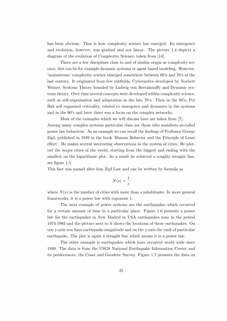
We consider earth species extinctions as a system, take the mass extinc-

tions through out the recorded history and plot them. On x-axis is the percent

of organism extinct during geological stage and on y-axis number of such stages

that occurred in the earth history. Here also manifests a power law shape.

The last example is a power spectrum of a traffic jam (Figure 1.9) on the

logarithmic plot. Research by the Kai Nagel and Maya Paczuszki in 1995.

As we see from those examples, there are many various systems which ex-

perience power law behaviour and in some cases it is a Zipf Law. Many other

examples could be recalled here. However, what is the important, is that power

laws are purely experimental law. They have been obtained by mere observa-

tion and joining the plot, there is no mathematical framework, theory that fully

explains those phenomenas.

1.4 Thesis outline

The thesis consist of five chapters and the appendix chapter, where the first was

an introduction.

28

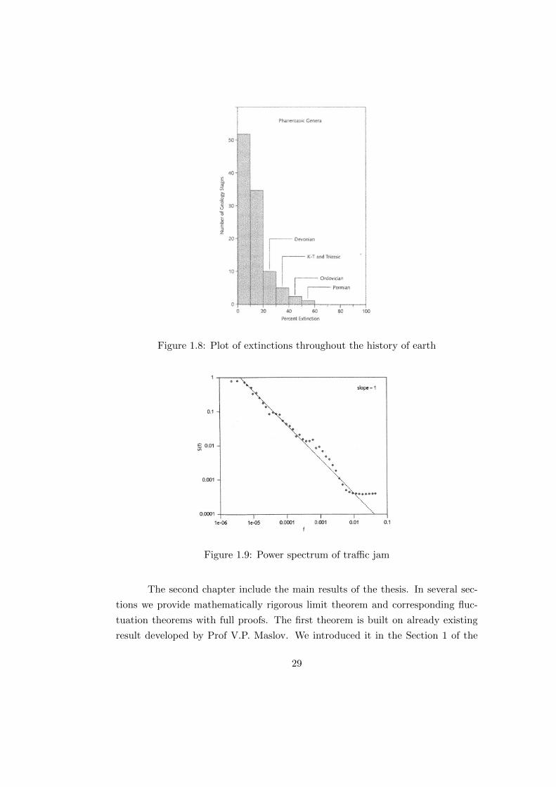
Figure 1.8: Plot of extinctions throughout the history of earth

Figure 1.9: Power spectrum of traffic jam

The second chapter include the main results of the thesis. In several sec-

tions we provide mathematically rigorous limit theorem and corresponding fluc-

tuation theorems with full proofs. The first theorem is built on already existing

result developed by Prof V.P. Maslov. We introduced it in the Section 1 of the

29

Introduction as Theorem 2. The ’new version’ we developed is a more rigorous

and precise extension of that result, with a mathematically rigorous proof. The

fluctuation theorems are the new results constructed on the fundaments of the

first theorem. The results of that chapter are in the phase of preparation for pub-

lishing.

In the third chapter we present several results which we developed spe-

cially for the proofs of the Chapter 2. It consists of solutions of some optimization

problems, some approximations and estimates. The results of this chapter are

mathematically rigorous with proofs provided. One result is given without proof

and is left for the future research.

The fourth chapter also is devoted for the results developed specifically for

the proofs of Chapter 2. It includes some extension of Laplace approximation put

in the few sections. These are new results however of minor relevancy. They were

constructed based on the Laplace approximation in the book [13].

Last chapter is devoted to conclusions, applications and future research.

We underline the contribution of our work to the field of Statistical Physics and

Complexity Science. A short section on possible application is included. Finally,

we emphasize possible future directions related to our work which can be con-

ducted, some ideas which came across during our research and possible extensions

of work already done.

In the Appendix we put all the well known results we used throughout the

thesis, some minor results are proved and some basic definitions are also recalled.

It consists of the Analysis, Probability, Asymptotics and Optimization.

30

2Limit theorems

In this chapter we introduce and prove the main results of the thesis. The limit

theorem and the corresponding fluctuation theorems.

We introduce a mathematical setting and all the assumptions on which the

results are based in the section one.

The content of the Section 2 is the limit theorem about the convergence of

the considered random variable to constant mean value. Corresponding estimate

of the speed of convergence are also included. This result is an extension and more

precise version of the Malsov Theorem , Theorem 2 in Introduction.

Next two sections are devoted to the fluctuation theorems. They provide

information on the distribution of deviation of considered random variable from

the maximum. As it turned out from the previous section there are two types of

means, depending on the initial assumptions. As a result there are two fluctuation

theorems. In Section 3 we have one case, when the mean is in the interior of the

sample space and in the Section 4 the mean is on the boundary.

In the last Section we provide some additional results, estimates, used in

proof the fluctuation theorems. For the transparency of the proofs we moved it

to a separate section.

2.1 Introduction

This section consists of a step by step introduction of the mathematical setting

which forms a background for the results of this thesis. Several assumption are

made on the way in order to simplify the setting and make construction of the

proofs possible.

For given integers G,N > 0, real number E > 0 and mapping

ε : 1, 2, . . . G → R we introduce a probability space. The elementary events

are uniformly distributed G-dimensional vectors of nonnegative integers ni, i =

31

1, . . . , G satisfying constraints:

N = n1 + n2 + . . .+ nG, (2.1)

EN ≥ ε(1)n1 + ε(2)n2 + . . .+ ε(G)nG. (2.2)

In physics we call such system micro-canonical ensemble.

Arbitrary elementary event can be illustrated as the random distribution

of N balls in G boxes. Moreover, each box has ’weight’ coefficient ε(i) and the

total ’weight’ must be less or equal EN .

Furthermore, let us denote the image of the function ε as the set ε1, ε2, . . . , εmand without loss of generality it can be ordered ε1 < ε2 < . . . < εm. To each ele-

ment in the set corresponds a positive integer Gi, i = 1, 2, . . . ,m representing the

number of points in the domain of ε having the values εi, so that G =∑m

i=1Gi.

We can use this setting to define probability space in an alternative way.

We consider the values Gi and εi, i = 1, . . . ,m instead of the mapping ε. Respec-

tively, the conditions (2.1) and (2.2) are reformulated

N = N1 +N2 + . . .+Nm, (2.3)

EN ≥ ε1N1 + ε2N2 + . . .+ εmNm, (2.4)

where Ni = nG1+...+Gi−1+1+. . .+nG1+...+Gi−1+2+nG1+...+Gi−1+Gi for i = 1, . . . ,m.

Vectors satisfying above conditions form a sample space which will be denoted by

ΩN,E . This situation, can be illustrated as distributing N balls over m

’bigger’ boxes, where to each corresponds unique value εi. Then in each i-th ’big-

ger’ box balls are distributed over Gi boxes.

For given vectors N = (N1, . . . , Nm) and G = (G1, . . . , Gm) the num-

ber of different combinations which can occur in such redistribution, exactly the

logarithm of that number is denoted by S(N ) and called Entropy.

We count those combinations using formula from Combinatorics for the

possible number of unordered arrangements of size r obtained by drawing from n

32

objects,

S(N ) = lnm∏i=1

(Ni +Gi − 1)!

Ni!(Gi − 1)!. (2.5)

Let us consider the discrete random vector denoted byXN = (X1, X2, . . . , Xm)

where Xi = Ni/N, i = 1, . . . ,m and respectively sample space given by trans-

formed conditions (2.3) and (2.4) is given by

1 = x1 + x2 + . . .+ xm,

E ≥ ε1x1 + ε2x2 + . . .+ εmxm, xi ∈

1

N,

2

N, . . . ,

N − 1

N, 1

,

and denoted by ΩE and respectively entropy function

S(x,N) = lnm∏i=1

(xiN +Gi − 1)!

(xiN)!(Gi − 1)!.

The probability mass function (pmf) of random variable X is given by

Pr(X = x) =1

Z(N,E)

m∏i=1

(xiN +Gi − 1)!

(xiN)!(Gi − 1)!, (2.6)

where Z(N,E) is a normalization constant specified by

Z(N,E) =∑ΩE

m∏i=1

(xiN +Gi − 1)!

(xiN)!(Gi − 1)!, (2.7)

which is a total number of elementary events in the sample space ΩE . Sometimes

Z(N,E) is called partition function.

We are interested in the behaviour of random vector X as N → ∞. We

consider a particular case when G = G(N) is an increasing function of N . More-

over, for each N the components Gi are equally weighted and their number m

remains constant. Which means that for all N , Gi = giG(N) for i = 1, . . . ,m and

some constants gi such that∑m

i=1 gi = 1.

We distinguish three cases of function G(N), depending on its asymptotic

33

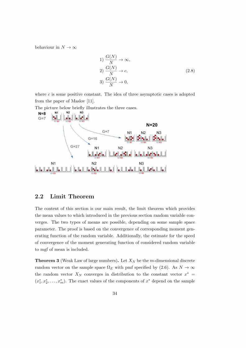
behaviour in N →∞

1)G(N)

N→∞,

2)G(N)

N→ c, (2.8)

3)G(N)

N→ 0,

where c is some positive constant. The idea of three asymptotic cases is adopted

from the paper of Maslov [11].

The picture below briefly illustrates the three cases.

2.2 Limit Theorem

The content of this section is our main result, the limit theorem which provides

the mean values to which introduced in the previous section random variable con-

verges. The two types of means are possible, depending on some sample space

parameter. The proof is based on the convergence of corresponding moment gen-

erating function of the random variable. Additionally, the estimate for the speed

of convergence of the moment generating function of considered random variable

to mgf of mean is included.

Theorem 3 (Weak Law of large numbers). Let XN be the m-dimensional discrete

random vector on the sample space ΩE with pmf specified by (2.6). As N → ∞the random vector XN converges in distribution to the constant vector x∗ =

(x∗1, x∗2, . . . , x

∗m). The exact values of the components of x∗ depend on the sample

34

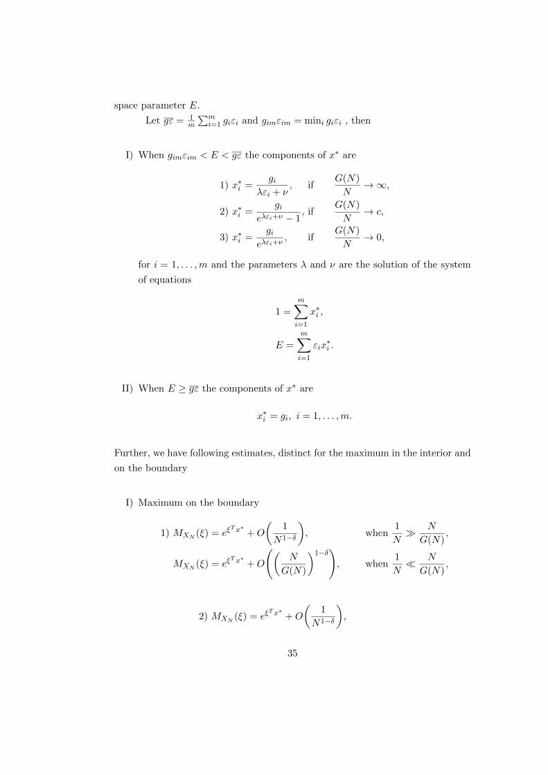
space parameter E.

Let gε = 1m

∑mi=1 giεi and gimεim = mini giεi , then

I) When gimεim < E < gε the components of x∗ are

1) x∗i =gi

λεi + ν, if

G(N)

N→∞,

2) x∗i =gi

eλεi+ν − 1, if

G(N)

N→ c,

3) x∗i =gi

eλεi+ν, if

G(N)

N→ 0,

for i = 1, . . . ,m and the parameters λ and ν are the solution of the system

of equations

1 =

m∑i=1

x∗i ,

E =

m∑i=1

εix∗i .

II) When E ≥ gε the components of x∗ are

x∗i = gi, i = 1, . . . ,m.

Further, we have following estimates, distinct for the maximum in the interior and

on the boundary

I) Maximum on the boundary

1) MXN (ξ) = eξT x∗ +O

(1

N1−δ

), when

1

N N

G(N),

MXN (ξ) = eξT x∗ +O

((N

G(N)

)1−δ), when

1

N N

G(N),


(1

N1−δ

),

35


(1

G(N)1−δ

), when

1

G(N) G(N)

N,


((G(N)

N

)1−δ), when

1

G(N) G(N)

N

as N →∞.

II) Maximum in the interior


(1√N

), when

1√N N

G(N),


((G(N)

N

)1−δ)), when

1√N N

G(N),


(1√N

),


(1√G(N)

), when

1√G(N)

G(N)

N,


((G(N)

N

)1−δ), when

1√G(N)

G(N)

N,

as N → ∞, valid for some arbitrary small constant δ, where MXN (ξ) is moment

generating function of the random vecto XN .

Proof. We prove the theorem by showing convergence of the moment generating

function of the random vector XN to a constant vector x∗ as N →∞.

The mgf of r.v. XN is equal

MX(ξ) = E[eξTX ].

Evaluating the probability mass function we obtain following expression for MX(ξ)

MX(ξ) =1

Z(N,E)

∑ΩE

eξT x

m∏i=1

(xiN +Gi − 1)!

(xiN)!(Gi − 1)!. (2.9)

We start with approximating the first part of MXN (ξ), i.e the normalization con-

36

stant Z(N,E), given by

Z(N,E) =∑ΩE

eS(x,N),

Let us consider only the first case of G(N), (2.8). We use Lemma 1 from Section

1 in the Chapter III

eS(x,N) = (2π)−m2 eNf1(x,N)+R1(N)

(1 +O

(1

N

)), N →∞

and then performing the summation over ΩE and applying Triangle inequality on

the LHS we get the following inequalities

Z(N,E) = (2π)−m2

∑ΩE

eNf1(x,N)+R1(N)

(1 +O

(1

N

)), N →∞. (2.10)

In the next step we approximate above sums using Lemma 7 from the Section 4

Ch.III∑ΩE

eNf1(x,N)+R1(N) =

∫ΩE

eNf1(x,N)+R1(N)dx

(1 +O

(1

N

)), N →∞,

and together with (2.10) we obtain

Z(N,E) = (2π)−m2

∫ΩE

eNf1(x,N)+R1(N)dx

(1 +O

(1

N

)), N →∞. (2.11)

Then from Lemma 2 Section 2.1 Ch.III we have that functions fl(x), l =

1, 2, 3 has two types of maximum depending on the sample space parameters E

and εi, i = 1, . . . ,m. It can be on the boundary of the domain of optimization or

in the interior of the domain. From the Lemma 3 in Section 2.2 of Chapter III,

the function fl(x,N) has a unique maximum, and as fl(x,N) → fl(x), N → ∞hence its maximum also is on the boundary of the domain or in the interior. For

those two cases separately we apply Extended Laplace approximation from the

Chapter IV.

I) When the maximum of fl(x,N) is attained on the boundary of the domain,

37

we use Theorem 8 from Section 3 Chapter IV and for the first case we have∫ΩE

eNf1(x,N)+R1(N)dx =

= eNf1(x∗(N),N)+R1(N) 1

N

(2π

N

)m−12 |f ′1(x∗(N), N)|−1√

| detD2f1(x∗(N), N)|

(1 +O

(1

N

)),

as N →∞, where x∗(N) is a maximal point of fl(x,N), l = 1, 2, 3.

Then we combine above approximations with (2.11) and obtain for all three

cases

1) Z(N,E) =

= eNf1(x∗(N),N)+R1(N) 1

2π

1

N

(1

N

)m−12 |f ′1(x∗(N), N)|−1√


(1 +O

(1

N

)),

2) Z(N,E) =

= eNf2(x∗(N),N)+R2(N) 1

2π

1

N

(1

N

)m−12 |f ′2(x∗(N), N)|−1√


(1 +O

(1

N

)),

3) Z(N,E) = eG(N)f3(x∗(N),N)+R3(N) 1

2π

1

G(N)

(1

G(N)

)m−12

×

× |f ′3(x∗(N), N)|−1√| detD2f3(x∗(N), N)|

(1 +O

(1

G(N)

)),

as N →∞, where in the second case the alteration from the first case is only

by the index of the function f1. For the third case the alteration is in the

index of f1 and function G(N) insted of N in th appriopriate places.

II) When the maximum of fl(x,N) is in the interior of the domain, we have the

Extended Laplace approximation for the first case∫ΩE

eNf1(x,N)+R1(N)dx =

= eNf1(x∗(N),N)+R1(N)

(2π

N

)m2 1√

detD2f1(x∗(N), N)

(1 +O

(1

N

)), N →∞

where x∗(N) is a maximal point.

38

Then we combine above approximations with (2.11) and obtain

1) Z(N,E) = eNf1(x∗(N),N)+R1(N)

(1

N

)m2 1√

detD2f1(x∗(N), N)

(1 +O

(1√N

)),

2) Z(N,E) = eNf2(x∗(N),N)+R2(N)

(1

N

)m2 1√

detD2f2(x∗(N), N)

(1 +O

(1√N

)),

3) Z(N,E) = eG(N)f3(x∗(N),N)+R3(N)

(1

G(N)

)m2

×

× 1√detD2f3(x∗(N), N)

(1 +O

(1√G(N)

)),

as N →∞.

Analogically we approximate the other part of the mgf (2.9). The additional

function under the sum does not affect the approximation of entropy nor the

approximation of sum with the integral. In the Extended Laplace approximation

this factor becomes function g in the Theorem. Hence we have

I) When the maximum x∗(N) is on the boundary of the domain we have

1)∑ΩE

eξT x+S(x,N) = eξ

T x∗(N)+Nf1(x∗(N),N)+R1(N) 1

2π

(1

N

)m−12

×

× |f ′1(x∗(N), N)|−1√| detD2f1(x∗(N), N)|

(1 +O

(1

N

)),

2)∑ΩE

eξT x+S(x,N) = eξ

T x∗(N)+Nf2(x∗(N),N)+R2(N) 1

2π

(1

N

)m−12

×

× |f ′2(x∗(N), N)|−1√| detD2f2(x∗(N), N)|

(1 +O

(1

N

)),

3)∑ΩE

eξT x+S(x,N) = eξ

T x∗(N)+G(N)f3(x∗(N),N)+R3(N) 1

2π

(1

G(N)

)m−12

×

× |f ′3(x∗(N), N)|−1√| detD2f3(x∗(N), N)|

(1 +O

(1

N

)),

as N →∞.

39

II) When the maximum is inside the domain than we have

1)∑ΩE

eξT x+S(x,N) = eξ

T x∗(N)+Nf1(x∗(N),N)+R1(N)

(1

N

)m2

×

× 1√detD2f1(x∗(N), N)

(1 +O

(1√N

)),

2)∑ΩE

eξT x+S(x,N) = eξ

T x∗(N)+Nf2(x∗(N),N)+R2(N)

(1

N

)m2

×

× 1√detD2f2(x∗(N), N)

(1 +O

(1√N

)),

3)∑ΩE

eξT x+S(x,N) = eξ

T x∗(N)+G(N)f3(x∗(N),N)+R3(N)

(1

G(N)

)m2

×

× 1√detD2f3(x∗(N), N)

(1 +O

(1√N

)),

as N →∞.

Finally, we put together the approximations of the first and second part of mgf

using Lemma 16 from the Appendix A.1 and cancel the identical terms. For two

types of maximum we have separately

I) Maximum is on the boundary of the domain

1) MXN (ξ) = eξT x∗(N)

(1 +O

(1

N

)),


(1 +O

(1

N

)), (2.12)


(1 +O

(1

G(N)

)),

as N →∞.

II) Maximum in the interior of the domain.

Here the situation is identical as for the boundary case but instead of N in

40

the RHS we have√N or

√G(N)


(1 +O

(1√N

)),


(1 +O

(1√N

)), (2.13)


(1 +O

(1√G(N)

)),

as N →∞.

Next we use following Taylor expansion

eξT x∗(N) = eξ

T x∗ + ξeξT xθ(x∗(N)− x∗), (2.14)

where x∗ is a maximum of limit functions of fl(x,N), l = 1, 2, 3 denoted by fl(x),

given by Lemma 2 of Section 2.1 of Chapter III.

Further we substitute approximation for (x∗(N)−x∗) given by Lemma 4 of Secion

3 in Chapter II and obtain

1) eξT x∗(N) = eξ

T x∗ + ξeξT xθO

(1

N1−δ

), when

1

N N

G(N),

eξT x∗(N) = eξ


((N

G(N)

)1−δ)), when

1

N N

G(N),



(1

N1−δ

),



(1

G(N)1−δ

), when

1

G(N) G(N)

N,

eξT x∗(N) = eξ


((G(N)

N

)1−δ)), when

1

G(N) G(N)

N,

as N →∞.

Now we combine it with approximations (2.12) and (2.13) for two cases of maxi-

mum

41

I) Maximum on the boundary

1) MXN (ξ) =

[eξT x∗ + ξeξ

T xθO

(1

N1−δ

)](1 +O

(1

N

)), when

1

N N

G(N),

MXN (ξ) =

[eξT x∗ + ξeξ

T xθO

((N

G(N)

)1−δ))](1 +O

(1

N

)), when

1

N N

G(N),

2) MXN (ξ) =

[eξT x∗ + ξeξ

T xθO

(1

N1−δ

)](1 +O

(1

N

)),

3) MXN (ξ) =

[eξT x∗ + ξeξ

T xθO

(1

G(N)1−δ

)](1 +O

(1

G(N)

)), when

1

G(N) G(N)

N,

MXN (ξ) =

[eξT x∗ + ξeξ

T xθO

((G(N)

N

)1−δ))](1 +O

(1

G(N)

)), when

1

G(N) G(N)

N,

as N →∞. Then we simplify above asymptotic equations and get


(1

N1−δ

), when

1

N N

G(N),


((N

G(N)

)1−δ), when

1

N N

G(N),


(1

N1−δ

),


(1

G(N)1−δ

)when

1

G(N) G(N)

N,


((G(N)

N

)1−δ), when

1

G(N) G(N)

N,

as N →∞, where δ is some arbitrary small positive constant. Therefore, we

get the final result for that case.

II) Maximum in the interior.

42

1) MXN (ξ) =

[eξT x∗ + ξeξ

T xθO

(1

N1−δ

)](1 +O

(1√N

)),

when1√N N

G(N),

MXN (ξ) =

[eξT x∗ + ξeξ

T xθO

((N

G(N)

)1−δ))](1 +O

(1√N

)),

when1√N√N

G(N),

2) MXN (ξ) =

[eξT x∗ + ξeξ

T xθO

(1

N1−δ

)](1 +O

(1√N

)),

3) MXN (ξ) =

[eξT x∗ + ξeξ

T xθO

(1

G(N)1−δ

)](1 +O

(1√G(N)

)),

when1√G(N)

G(N)

N,

MXN (ξ) =

[eξT x∗ + ξeξ

T xθO

((G(N)

N

)1−δ))](1 +O

(1√G(N)

)),

when1√G(N)

G(N)

N,

as N →∞ and after simplification of above equation we get


(1√N

), when

1√N N

G(N),


((N

G(N)

)1−δ), when

1√N N

G(N),


(1√N

),


(1√G(N)

)when

1√G(N)

G(N)

N,


((G(N)

N

)1−δ), when

1√G(N)

G(N)

N,

as N →∞, which is our final result.

43

2.3 Fluctuation theorem, maximum in the interior of

the domain

The fluctuation of the random variable from the mean value is introduced and

proved in this section, the case when the maximum/mean is in the interior of the

domain. As in the previous limit theorem the proof is based on the convergence

of the moment generating functions. The speed of convergence of corresponding

moment generating functions are included.

Theorem 4. For each case G(N) given by (2.8) we have a m-dimensional random

vector YN such that

1) YN =√N(XN − x∗),

2) YN =√N(XN − x∗),

3) YN =√G(N)(XN − x∗),

defined on the discrete sample space ΩE with pmf specified by (2.6).

Then for the sample space parameter E ≥ gε, as N → ∞ the distribution of the

random vector Y converges to the multivariate normal N (0,−D2fl(x∗)−1), where

l = 1, 2, 3 indicates the case of G(N).

Furthermore, we have estimates

1) MYN (ξ) = e12ξTD2f1(x∗)−1ξ +O

(1

N1/2−δ

), when

1

N N

G(N),

MYN (ξ) = e12ξTD2f1(x∗)−1ξ +O

(N3/2−δ

G(N)1−δ

), when

1√N N

G(N),

2) MYN (ξ) = e12ξTD2f2(x∗)−1ξ +O

(1

N1/2−δ

),

3) MYN (ξ) = e12ξTD2f3(x∗)−1ξ +O

(1

G(N)1/2−δ

), when

1

G(N) G(N)

N,

MYN (ξ) = e12ξTD2f3(x∗)−1ξ +O

(G(N)3/2−δ

N1−δ

), when

1√G(N)

G(N)

N,

as N →∞, where δ is some arbitrary small constant.

Proof. The approach is analogical to the the proof in the previous section.

We first approximate the numerator and denominator of the mgf of YN using

44

Lemma 1 from Section 1, Ch. III, then Lemma 7 from the Section 4, Ch. III.

Since the E ≥ gε from Lemma 2 Section 3, Ch.III we deduce that maximum

of the approximated function is in the interior of the domain. Therefore we use

appropriate Laplace approximation, Theorem 8, Section 2, Chapter IV. Finally we

combine both approximations, for the numerator and denominator using Lemma

16 from the Appendix A.1. As a result we obtain following estimates

1)

∣∣∣∣MYN (ξ)− eN(f1(x∗(N),N)−f1(x∗(N),N))

√detD2f1(x∗(N), N)√detD2f1(x∗(N), N)

∣∣∣∣ ≤≤ Ki

1

1√NeN(f1(x∗(N),N)−f1(x∗(N),N))


,

2)

∣∣∣∣MYN (ξ)− eN(f2(x∗(N),N)−f2(x∗(N),N))


∣∣∣∣ ≤≤ Ki

2

1√NeN(f2(x∗(N),N)−f2(x∗(N),N))


,

3)

∣∣∣∣MYN (ξ)− eG(N)(f3(x∗(N),N)−f3(x∗(N),N))


∣∣∣∣ ≤≤ Ki

3

1√G(N)

eG(N)(f3(x∗(N),N)−f3(x∗(N),N))


, (2.15)

where fl(x,N) = f(x,N) + 1√NξT (x − x∗) for l = 1, 2 and fl(x,N) = f(x,N) +

1√G(N)

ξT (x − x∗) for l = 3 and x∗(N) is a maximum of f(x,N). Next, we use

the result of the Proposition 2 from Section 5 of this Chapter and multiply it by

exp(N(f1(x∗(N), N)− f1(x∗(N), N))) to get

1)

∣∣∣∣eN(f1(x∗(N),N)−f1(x∗(N),N))


− eN(f1(x∗(N),N)−f1(x∗(N),N))

∣∣∣∣ ≤≤ Kii

1

1√NeN(f1(x∗(N),N)−f1(x∗(N),N)),

45

2)

∣∣∣∣eN(f2(x∗(N),N)−f2(x∗(N),N))


− eN(f2(x∗(N),N)−f2(x∗(N),N))

∣∣∣∣ ≤≤ Kii

2

1√NeN(f2(x∗(N),N)−f2(x∗(N),N))

3)

∣∣∣∣eG(N)(f3(x∗(N),N)−f3(x∗(N),N))


− eG(N)(f3(x∗(N),N)−f3(x∗(N),N))

∣∣∣∣ ≤≤ Kii

3

1√G(N)

eG(N)(f3(x∗(N),N)−f3(x∗(N),N)),

and combine above result with (2.15) and get

1)

∣∣∣∣MYN (ξ)− eN(f1(x∗(N),N)−f1(x∗(N),N))

∣∣∣∣ ≤ Kiii1

1√NeN(f1(x∗(N),N)−f1(x∗(N),N)),

2)

∣∣∣∣MYN (ξ)− eN(f2(x∗(N),N)−f2(x∗(N),N))

∣∣∣∣ ≤ Kiii2

1√NeN(f2(x∗(N),N)−f2(x∗(N),N)),

3)

∣∣∣∣MYN (ξ)− eG(N)(f3(x∗(N),N)−f3(x∗(N),N))

∣∣∣∣ ≤ Kiii3

1√G(N)

eG(N)(f3(x∗(N),N)−f3(x∗(N),N)),

where

1) Kiii1 = Kii

1 +Ki1

(1 +

Kii1√N

),

2) Kiii2 = Kii

2 +Ki2

(1 +

Kii2√N

),

3) Kiii3 = Kii

3 +Ki3

(1 +

Kii3√

G(N)

).

Now we use Proposition 1 from the Section 5 to approximate the expression in

the exponent

1) N(f1(x∗(N), N)− f1(x∗(N), N)) =√N(x∗(N)− x∗)T

(ξ +

ξD⊗3f1(xθ(N), N)ξ√N

)+

+1

2ξTD2f1(x∗)−1ξ +

1√N

(φ+

ξTκ′ξ

2√N

).

46

2) N(f2(x∗(N), N)− f2(x∗(N), N)) =√N(x∗(N)− x∗)T

(ξ +


)+

+1

2ξTD2f2(x∗)−1ξ +

1√N

(φ+

ξTκ′ξ

2√N

).

3) G(N)(f3(x∗(N), N)− f3(x∗(N), N)) =√G(N)(x∗(N)− x∗)T

(ξ +

ξD⊗3f3(xθ(N), N)ξ√G(N)

)+

+1

2ξTD2f3(x∗)−1ξ +

1√G(N)

(φ+

ξTκ′ξ

2√G(N)

). (2.16)

Then we approximate the expression (x∗(N)−x∗). From the Proposition 3 Section

4 Ch.III we have for all three cases

1. G(N)N →∞

x∗(N)− x∗ = K1N−1+δ, when

1

N N

G(N),

x∗(N)− x∗ = K1

(N

G(N)

)1−δ, when

1

N N

G(N).

2. G(N)N → c

x∗(N)− x∗ = K2N−1+δ.

3. G(N)N → 0

x∗(N)− x∗ = K3G(N)−1+δ, when1

G(N) G(N)

N,

x∗(N)− x∗ = K3

(G(N)

N

)1−δ, when

1

G(N) G(N)

N,

where the form of approximations is different and |Kl| ≤ 1, l = 1, 2, 3. Then we

47

substitute above estimates into (2.16) and after some rearrangements we have

1) N(f1(x∗(N), N)− f1(x∗(N), N)) =1

2ξTD2f1(x∗)−1ξ+

+1

N1/2−δ

(K1ξ +K1


+1

N δφ+

1

N δ

ξTκ′ξ

2√N

),when

1

N N

G(N),

N(f1(x∗(N), N)− f1(x∗(N), N)) =1


+N3/2−δ

G(N)1−δ

(K1ξ +K1


+G(N)1−δ

N2−δ

(φ+

ξTκ′ξ

2√N

)),when

1√N N

G(N),

2) N(f2(x∗(N), N)− f2(x∗(N), N)) =1


+1

N1/2−δ

(ξ +


+1

N δφ+

1

N δ

ξTκ′ξ

2√N

).

3) G(N)(f3(x∗(N), N)− f3(x∗(N), N)) =1


+1

G(N)1/2−δ

(K3ξ +K3


+1

G(N)δφ+

1

G(N)δξTκ′ξ

2√G(N)

),

when1

G(N) G(N)

N,

G(N)(f3(x∗(N), N)− f3(x∗(N), N)) =1


+G(N)3/2−δ

N1−δ

(K3ξ +K3


+N1−δ

G(N)2−δ

(φ+

ξTκ′ξ

2√G(N)

)),

when1√G(N)

G(N)

N,

where we omitted the case when 1√G(N)

G(N)N as the remainder would overcome

the term 12ξTD2f3(x∗)−1ξ which would contradict the theorem.

48

Then we introduce constants Kiv1 ,K

iv2 ,K

iv3 and exponentiate the expressions

1) eN(f1(x∗(N),N)−f1(x∗(N),N)) = e12ξTD2f1(x∗)−1ξ+N−1/2+δKiv

1 ,

when1

N N

G(N),

eN(f1(x∗(N),N)−f1(x∗(N),N)) = e12ξTD2f1(x∗)−1ξ+ N3/2−δ

G(N)1−δKiv

1 ,

when1√N N

G(N),

2) eN(f2(x∗(N),N)−f2(x∗(N),N)) = e12ξTD2f2(x∗)−1ξ+N−1/2+δKiv

2 .

3) eG(N)(f3(x∗(N),N)−f3(x∗(N),N)) = e12ξTD2f3(x∗)−1ξ+G(N)−1/2+δKiv

3 ,

when1

G(N) G(N)

N,

eG(N)(f3(x∗(N),N)−f3(x∗(N),N)) = e12ξTD2f3(x∗)−1ξ+

G(N)3/2−δ

N1−δ Kiv3 ,

when1√G(N)

G(N)

N.

Further, we take Taylor approximation of the RHS at the point e12ξTD2f3(x∗)−1ξ

and consequently obtain

1)∣∣∣eN(f1(x∗(N),N)−f1(x∗(N),N)) − e

12ξTD2f1(x∗)−1ξ

∣∣∣ =

=|Kiv

1 |N1/2−δ e

12ξTD2f1(x∗)−1ξ+θNN

−1/2+δKiv1 ,

when1

N N

G(N),∣∣∣eN(f1(x∗(N),N)−f1(x∗(N),N)) − e


∣∣∣ =

=N3/2−δ

G(N)1−δ |Kiv1 |e

12ξTD2f1(x∗)−1ξ+θN

N3/2−δG(N)1−δ

Kiv1 ,

when1√N N

G(N),

49

2)∣∣∣eN(f2(x∗(N),N)−f2(x∗(N),N)) − e


∣∣∣ =

=Kiv

2

N1/2−δ e12ξTD2f2(x∗)−1ξ+θNN

−1/2+δKiv1 ,

3)∣∣∣eG(N)(f3(x∗(N),N)−f3(x∗(N),N)) − e


∣∣∣ =

=Kiv

3

G(N)1/2−δ e12ξTD2f3(x∗)−1ξ+θNG(N)−1/2+δKiv

3 ,

when1

G(N) G(N)

N,∣∣∣eG(N)(f3(x∗(N),N)−f3(x∗(N),N)) − e


∣∣∣ =

=G(N)3/2−δ

N1−δ Kiv3 e

12ξTD2f3(x∗)−1ξ+θN

G(N)3/2−δ

N1−δ Kiv3 ,

when1√G(N)

G(N)

N,

and we introduce constants Kv1 ,K

v2 ,K

v3 such that

1)∣∣∣eN(f1(x∗(N),N)−f1(x∗(N),N)) − e


∣∣∣ =Kv

1

N1/2−δ ,

when1

N N

G(N),∣∣∣eN(f1(x∗(N),N)−f1(x∗(N),N)) − e


∣∣∣ =N3/2−δ

G(N)1−δKv1 ,

when1√N N

G(N),

2)∣∣∣eN(f2(x∗(N),N)−f2(x∗(N),N)) − e


∣∣∣ =Kv

2

N1/2−δ ,

50

3)∣∣∣eG(N)(f3(x∗(N),N)−f3(x∗(N),N)) − e


∣∣∣ =Kv

3

G(N)1/2−δ ,

when1

G(N) G(N)

N,∣∣∣eG(N)(f3(x∗(N),N)−f3(x∗(N),N)) − e


∣∣∣ =G(N)3/2−δ

N1−δ Kv3 ,

when1√G(N)

G(N)

N.

Now combine above estimates with (2.15) and as a result we get

1)∣∣∣MYN (ξ)− e


∣∣∣ =K1

N1/2−δ , when1

N N

G(N),∣∣∣MYN (ξ)− e


∣∣∣ =N3/2−δ

G(N)1−δK1,when1√N N

G(N),

2)∣∣∣MYN (ξ)− e


∣∣∣ =K2

N1/2−δ ,

3)∣∣∣MYN (ξ)− e


∣∣∣ =K3

G(N)1/2−δ , when1

G(N) G(N)

N,∣∣∣MYN (ξ)− e


∣∣∣ =G(N)3/2−δ

N1−δ K3,when1√G(N)

G(N)

N,

where the constants are equal

1) K1 = Kv1 +

1

N δKiii

1

(e

12ξTD2f1(x∗)−1ξ +

Kv1

N1/2−δ

),when

1

N N

G(N),

K1 = Kv1 +

G(N)1−δ

N2−δ Kiii1

(e

12ξTD2f1(x∗)−1ξ +

N3/2−δ

G(N)1−δKv1

),

when1√N N

G(N),

2) K2 = Kv2 +

1

N δKiii

2

(e

12ξTD2f2(x∗)−1ξ +

Kv2

N1/2−δ

),

51

3) K3 = Kv3 +

1

G(N)δKiii

3

(e

12ξTD2f3(x∗)−1ξ +

Kv3

G(N)1/2−δ

),when

1

G(N) G(N)

N,

K3 = Kv3 +

N1−δ

G(N)2−δKiii3

(e

12ξTD2f3(x∗)−1ξ +

G(N)3/2−δ

N1−δ Kv3

),

when1√G(N)

G(N)

N.

2.4 Fluctuation theorem, maximum on the boundary

of the domain

The case of fluctuation theorem, when mean is on the boundary of the sample

space is a content of this section. As previously, the proofs are done through

convergence of the mgfs. Also, the estimates for the speed of convergence to the

limiting distribution is included.

Theorem 5. For each case G(N) given by (2.8) we have a m-dimensional random

vector YN such that

1) YN = N(X1 − x∗1) +√N(XN − x∗),

2) YN = N(X1 − x∗1) +√N(XN − x∗),

3) YN = G(N)(X1 − x∗1) +√G(N)(XN − x∗),

defined on the discrete sample space ΩE with pmf specified by (2.6), where x =

(x1, x).

Then for sample space parameter gimεim < E < gε, as N → ∞ the distribution

of the random vector Y converges to the mixture of the multivariate normal along

x and exponential distribution along x1.

52

Furthermore, we have estimates

1) MYN (ξ) =|f ′1(x∗)||f ′1(x∗) + ξ|

e12ξTD2f1(x∗)−1ξ +O

(1

N1/2−δ

),

when1

N N

G(N),

MYN (ξ) =|f ′1(x∗)||f ′1(x∗) + ξ|


(N3/2−δ

G(N)1−δ

),

when1√N N

G(N),

2) MYN (ξ) =|f ′2(x∗)||f ′2(x∗) + ξ|


(1

N1/2−δ

),

3) MYN (ξ) =|f ′3(x∗)||f ′3(x∗) + ξ|


(1

G(N)1/2−δ

),

when1

G(N) G(N)

N,

MYN (ξ) =|f ′3(x∗)||f ′3(x∗) + ξ|


(G(N)3/2−δ

N1−δ

),

when1√G(N)

G(N)

N,

as N → ∞, where f ′l (x∗) is first derivative w.r.t. x1 and D2fl(x

∗) is m − 1-

dimensional matrix of second order derivatives w.r.t. x.

Proof. The approach of proving is similar as in the proof of the previous limit

theorems.

We approximate the numerator and the denominator of the mgf with appropriate

theorems and lemmas and eventually obtain

1)

∣∣∣∣MYN (ξ)− eN(f1(x∗(N),N)−f1(x∗(N),N)) |f ′1(x∗(N), N)||f ′1(x∗(N), N) + ξ|


∣∣∣∣ ≤≤ Ki

1

1√NeN(f1(x∗(N),N)−f1(x∗(N),N)) |f ′1(x∗(N), N)|

|f ′1(x∗(N), N) + ξ|


,

53

2)

∣∣∣∣MYN (ξ)− eN(f2(x∗(N),N)−f2(x∗(N),N)) |f ′2(x∗(N), N)||f ′2(x∗(N), N) + ξ|


∣∣∣∣ ≤≤ Ki

2

1√NeN(f2(x∗(N),N)−f2(x∗(N),N)) |f ′2(x∗(N), N)|

|f ′2(x∗(N), N) + ξ|


,

3)

∣∣∣∣MYN (ξ)− eG(N)(f3(x∗(N),N)−f3(x∗(N),N)) |f ′3(x∗(N), N)||f ′3(x∗(N), N) + ξ|


∣∣∣∣ ≤≤ Ki

3

1√G(N)

|f ′3(x∗(N), N)||f ′3(x∗(N), N) + ξ|

eG(N)(f3(x∗(N),N)−f3(x∗(N),N))


.

(2.17)

where fl(x,N) = fl(x,N) +N(X1 − x∗1) +√N(XN − x∗) and with G(N) for the

third case. Then the determinants are approximated analogically to previous limit

theorem, using Proposition 2 from Section 5.

Since the maximum along x1 has no dependence on N , component N(X1 − x∗)in the function fl(x,N) vanish and we can approximate the expression in the

exponents similarly as for the previous fluctuation theorem, i.e. by Proposition 1

from Section 5. Hence, we get

1)∣∣∣MYN (ξ)− |f ′1(x∗(N), N)|

|f ′1(x∗(N), N) + ξ|e


∣∣∣ ≤ Kii1

1

N1/2−δ|f ′1(x∗(N), N)||f ′1(x∗(N), N) + ξ|

,

when1

N N

G(N),∣∣∣MYN (ξ)− |f ′1(x∗(N), N)|

|f ′1(x∗(N), N) + ξ|e


∣∣∣ ≤ Kii1

N3/2−δ

G(N)1−δ|f ′1(x∗(N), N)||f ′1(x∗(N), N) + ξ|

,

when1√N N

G(N),

2)∣∣∣MYN (ξ)− |f ′2(x∗(N), N)|

|f ′2(x∗(N), N) + ξ|e


∣∣∣ ≤ Kii2

1

N1/2−δ|f ′2(x∗(N), N)||f ′2(x∗(N), N) + ξ|

,

54

3)∣∣∣MYN (ξ)− |f ′3(x∗(N), N)|

|f ′3(x∗(N), N) + ξ|e


∣∣∣ ≤ Kii3

1

G(N)1/2−δ|f ′3(x∗(N), N)||f ′3(x∗(N), N) + ξ|

,

when1

G(N) G(N)

N,∣∣∣MYN (ξ)− |f ′3(x∗(N), N)|

|f ′3(x∗(N), N) + ξ|e


∣∣∣ ≤ Kii3

G(N)3/2−δ

N1−δ|f ′3(x∗(N), N)||f ′3(x∗(N), N) + ξ|

,

when1√G(N)

G(N)

N.

Since the first derivative is along x1 and function fl is of the form fl(x,N) =∑mi=1 f(xi, N), and maximum along x1 is independent ofN we have f ′3(x∗(N), N) =

f ′3(x∗, N) and f ′3(x∗(N), N) = f ′3(x∗, N) . Further, using the Proposition 4 from

the Section 3 of Chapter III we have estimate

|f ′l (x∗(N), N)||f ′l (x∗(N), N) + ξ|

=|f ′l (x∗) +

KiiilN |

|f ′l (x∗) +KiiilN + ξ|

,

which after some manipulations is equal

|f ′l (x∗(N), N)||f ′l (x∗(N), N) + ξ|

=|f ′l (x∗)||f ′l (x∗) + ξ|

+Kivl

1

N,

valid for first two cases and for the third we have

|f ′3(x∗(N), N)||f ′3(x∗(N), N) + ξ|

=|f ′3(x∗)||f ′3(x∗) + ξ|

+Kivl

1

G(N).

Then we substitute above estimates into main estimate and get

1)∣∣∣MYN (ξ)− |f ′1(x∗)|

|f ′1(x∗) + ξ|e


∣∣∣ ≤ K11

N1/2−δ ,

when1

N N

G(N),∣∣∣MYN (ξ)− |f ′1(x∗)|

|f ′1(x∗) + ξ|e


∣∣∣ ≤ K1N3/2−δ

G(N)1−δ ,

when1√N N

G(N),

55

2)∣∣∣MYN (ξ)− |f ′2(x∗)|

|f ′2(x∗) + ξ|e


∣∣∣ ≤ K21

N1/2−δ ,

3)∣∣∣MYN (ξ)− |f ′3(x∗)|

|f ′3(x∗) + ξ|e


∣∣∣ ≤ K31

G(N)1/2−δ ,

when1

G(N) G(N)

N,∣∣∣MYN (ξ)− |f ′3(x∗)|

|f ′3(x∗) + ξ|e


∣∣∣ ≤ K3G(N)3/2−δ

N1−δ ,

when1√G(N)

G(N)

N,

where constants K1,K2,K3 are

1) K1 = Kii1

|f ′1(x∗)||f ′1(x∗) + ξ|

+Kiv1

1

N1/2+δe

12ξTD2f1(x∗)−1ξ +

Kii1 K

iv1

N,

when1

N N

G(N),

K1 = Kii1

|f ′1(x∗)||f ′1(x∗) + ξ|

+Kiv1

G(N)1−δ

N5/2−δ e12ξTD2f1(x∗)−1ξ +

Kii1 K

iv1

N,

when1√N N

G(N),

2) K2 = Kii2

|f ′2(x∗)||f ′2(x∗) + ξ|

+Kiv2

1

N1/2+δe

12ξTD2f2(x∗)−1ξ +

Kii2 K

iv2

N,

3) K3 = Kii3

|f ′3(x∗)||f ′3(x∗) + ξ|

+Kiv3

1

G(N)1/2+δe

12ξTD2f3(x∗)−1ξ +

Kii3 K

iv3

G(N),

when1

G(N) G(N)

N,

K3 = Kii3

|f ′3(x∗)||f ′3(x∗) + ξ|

+Kiv3

N1−δ

G(N)5/2−δ e12ξTD2f3(x∗)−1ξ +

Kii3 K

iv3

G(N),

when1√G(N)

G(N)

N,

hence we get the final result.

56

2.5 Related results

This section is devoted to some related estimated, used in the previous two section.

It is separated from the rest for the transparency of the proof.

Proposition 1. For the function fl(x,N) : Ω × N → R, l = 1, 2, 3, which has a

unique maximum at the critical point x∗(N) over the domain Ω ∈ Rm, we have

another function defined for each case of (2.8)

1) f1(x,N) = f(x,N) +1√N

(x− x∗)T ξ,

2) f2(x,N) = f(x,N) +1√N

(x− x∗)T ξ,

3) f3(x,N) = f(x,N) +1√G(N)

(x− x∗)T ξ,

where ξ has a value from the neighborhood of 0 and x∗ ∈ Ω. Then we have

following estimates

1) x∗(N)− x∗(N) = D2f1(x∗(N), N)−1 ξ√N

+εNN,

|εN | ≤F

(3)xθ(

F′(2)x∗(N)

)3(|ξ|+ F 3xθ

N1/6

),

2) x∗(N)− x∗(N) = D2f2(x∗(N), N)−1 ξ√N

+εNN,

|εN | ≤F

(3)xθ(

F′(2)x∗(N)

)3(|ξ|+ F 3xθ

N1/6

),

3) x∗(N)− x∗(N) = D2f3(x∗(N), N)−1 ξ√G(N)

+εN

G(N),

|εN | ≤F

(3)xθ(

F′(2)x∗(N)

)3(|ξ|+ F 3xθ

G(N)1/6

),

where x∗(N) is maximum of the function f(x,N).

57

Further, we have estimates

1) f1(x∗(N), N)− f1(x∗(N), N) =1√N

(x∗(N)− x∗)T(ξ +


)+

+1

2NξTD2f1(x∗)−1ξ +

1

N3/2

(φ+

ξTκ′ξ

2√N

).

2) f2(x∗(N), N)− f2(x∗(N), N) =1√N

(x∗(N)− x∗)T(ξ +


)+

+1

2NξTD2f2(x∗)−1ξ +

1

N3/2

(φ+

ξTκ′ξ

2√N

).

3) f3(x∗(N), N)− f3(x∗(N), N) =1√G(N)

(x∗(N)− x∗)T(ξ +


)+

+1

2G(N)ξTD2f3(x∗)−1ξ +

1

G(N)3/2

(φ+

ξTκ′ξ

2√G(N)

).

where

1) |φ| ≤ F(3)xθ

6

∣∣∣∣D2f1(x∗(N), N)−1ξ +εN√N

∣∣∣∣3 +

∣∣∣∣2εTNξ +1

2N1/2εTND

2f1(x∗(N), N)εN

∣∣∣∣,2) |φ| ≤ F

(3)xθ

6

∣∣∣∣D2f2(x∗(N), N)−1ξ +εN√N

∣∣∣∣3 +

∣∣∣∣2εTNξ +1

2N1/2εTND

2f2(x∗(N), N)εN

∣∣∣∣,3) |φ| ≤ F

(3)xθ

6

∣∣∣∣D2f3(x∗(N), N)−1ξ +εN√G(N)

∣∣∣∣3 +

∣∣∣∣2εTNξ +1

2G(N)1/2εTND

2f3(x∗(N), N)εN

∣∣∣∣Proof. First we prove for the case 1) and 2) of G(N) and we drop the index of

case in f temporally. Let us take some xB such that |xB−x∗(N)| = N−1/3. Then

we approximate Df(x,N) with first order Taylor expansion at x∗(N)

Df(x,N) = Df(x∗(N), N) +D2f(xθ(N))T (x− x∗(N)).

Since x∗(N) is a critical point, Df(x∗(N), N) = o. Taking the upper bound of

the above expansion, together with the absolute value applied on both sided gives

|Df(x,N)| ≥ F ′(2)xθ(N)|x− x

∗(N)|,

58

and for the point xB we have

|Df(xB, N)| ≥F′(2)xθ(N)

N1/3. (2.18)

Further, for the maximum x∗(N) we have

Df(x∗(N), N) +ξ√N

= o,

hence, after changing the side of second term and applying absolute value on the

both sides we obtain

|Df(x∗(N), N)| = |ξ|√N, (2.19)

Since f ∈ C2 and detD2f(x∗(N,N)) 6= 0, by the inverse function theorem we have

that the mapping M : x → Df(x,N) is invertible in the neighborhood of x∗(N)

and the inverse function is in the class C1. Hence, from the estimates (2.18) and

(2.19) together with Df(x∗(N), N) = o and knowing that |xB − x∗(N)| = N−1/3

we can infer following estimate

|x∗(N)− x∗(N)| ≤ N−1/3. (2.20)

Further we use second order Taylor expansion of Df(x∗(N), N) at x∗(N)

Df(x∗(N), N) =Df(x∗(N), N)− ξ√N

+D2f(x∗(N), N)T (x∗(N)− x∗(N))+

(2.21)

+D3f(xθ(N))(x∗(N)− x∗(N))⊗2,

where xθ(N) is some point between x∗(N) and x∗(N). Notice, that asDf(x∗(N), N) =

o and Df(x∗(N), N) = o.

Now we get the upper bound of expansion (2.21) and apply absolute value on both

sides∣∣∣∣D2f(x∗(N), N)T (x∗(N)− x∗(N))− ξ√N

∣∣∣∣ ≤ F (3)xθ(N)|x

∗(N)− x∗(N)|2, (2.22)

59

and use estimate (2.20)∣∣∣∣D2f(x∗(N), N)T (x∗(N)− x∗(N))− ξ√N

∣∣∣∣ ≤ F (3)xθ(N)N

−2/3. (2.23)

Next we get the lower bound for (2.21)∣∣∣∣D2f(x∗(N), N)T (x∗(N)− x∗(N))− ξ√N

∣∣∣∣ ≥ F ′(2)x∗(N)|x

∗(N)− x∗(N)| −∣∣∣∣ ξ√N

∣∣∣∣.(2.24)

Next, we combine upper (2.23) and lower bound (2.24) into one inequality

F′(2)x∗(N)|x

∗(N)− x∗(N)| −∣∣∣∣ ξ√N

∣∣∣∣ ≤ F (3)xθ(N)N

−2/3,

and after some manipulations one get estimate

|x∗(N)− x∗(N)| ≤

(F′(2)x∗(N)

)−1

√N

(|ξ|+ F

(3)xθ(N)N

−1/6

),

Next we substitute above estimate into (2.22)

∣∣∣∣D2f(x∗(N), N)T (x∗(N)−x∗(N))− ξ√N

∣∣∣∣ ≤ F(3)xθ(N)

(F′(2)x∗(N)

)−2

N

(|ξ|+F (3)

xθ(N)N−1/6

)2

.

(2.25)

Further, we transform the LHS of the inequality∣∣∣∣D2f(x∗(N), N)T (x∗(N)− x∗(N))− ξ√N

∣∣∣∣ =

=

∣∣∣∣D2f(x∗(N), N)T (x∗(N)− x∗(N))−D2f(x∗(N), N)T(D2f(x∗(N), N)T

)−1 ξ√N

∣∣∣∣ =

=

∣∣∣∣D2f(x∗(N), N)T(

(x∗(N)− x∗(N))−(D2f(x∗(N), N)T

)−1 ξ√N

)∣∣∣∣,calculate the lower bound of it∣∣∣∣D2f(x∗(N), N)T

((x∗(N)− x∗(N))−

(D2f(x∗(N), N)T

)−1 ξ√N

)∣∣∣∣ ≥≥ F ′(2)

x∗(N)

∣∣∣∣(x∗(N)− x∗(N))−(D2f(x∗(N), N)T

)−1 ξ√N

∣∣∣∣

60

and substitute back into (2.25) and dividing by F′(2)x∗(N)∣∣∣∣x∗(N)− x∗(N)−

(D2f(x∗(N), N)T

)−1 ξ√N

∣∣∣∣ ≤≤ 1

NF

(3)xθ(N)

(F′(2)x∗(N)

)−3(|ξ|+ F

(3)xθ(N)N

−1/6

)2

.

Since D2f(x∗(N), N) is a matrix of second derivatives of the continuous function

D2f(x∗(N), N)T = D2f(x∗(N), N), hence we get the first result of the theorem,

i.e

x∗(N) =x∗(N) +D2f(x∗(N), N)−1 ξ√N

+εNN,

|εN | ≤F

(3)xθ(N)(

F′(2)x∗(N)

)3(|ξ|+ F(3)xθ(n)

N1/6

),

Now, we derive the second result of the theorem. We substitute the above estimate

into f(x∗(N), N), expand the function using 3-rd order Taylor expansion at x∗(N)

and apply absolute value

f(x∗(N), N) = f

(x∗(N) +D2f(x∗(N), N)−1 ξ√

N+εNN,N

)=

= f(x∗(N), N) +Df(x∗(N), N)

(D2f(x∗(N), N)−1 ξ√

N+εNN

)+

+1

2

(D2f(x∗(N), N)−1 ξ√

N+εNN

)TD2f(x∗(N), N)

(D2f(x∗(N), N)−1 ξ√

N+εNN

)+

+1

6

⟨D⊗3f(xθ(N), N),

(D2f(x∗(N), N)−1 ξ√

N+εNN

)⊗3⟩,

where xθ(N) is somwhere between x∗(N) and x∗(N).

61

Then we change side of some terms and apply absolute value∣∣∣∣∣f(x∗(N), N) = f

(x∗(N) +D2f(x∗(N), N)−1 ξ√

N+εNN,N

)= −

− f(x∗(N), N)−Df(x∗(N), N)

(D2f(x∗(N), N)−1 ξ√

N+εNN

)−

− 1

2

(D2f(x∗(N), N)−1 ξ√

N+εNN

)TD2f(x∗(N), N)

(D2f(x∗(N), N)−1 ξ√

N+εNN

)−

− 1

6

⟨D⊗3f(θ(N), N),

(D2f(x∗(N), N)−1 ξ√

N+εNN

)⊗3⟩∣∣∣∣∣ = 0,

and we calculate the upper bound and as Df(x∗(N), N) = o we have∣∣∣∣∣f(x∗(N), N)− f(x∗(N), N)−

− 1

2

(D2f(x∗(N), N)−1 ξ√

N+εNN

)TD2f(x∗(N), N)

(D2f(x∗(N), N)−1 ξ√

N+εNN

)∣∣∣∣∣ ≤≤ F

(3)xθ

6

∣∣∣∣D2f(x∗(N), N)−1 ξ√N

+εNN

∣∣∣∣3,consequently after some manipulations we get∣∣∣∣f(x∗(N), N)− f(x∗(N), N)− 1

2NξTD2f(x∗(N), N)−1ξ − 1

N3/2εTNξ−

− 1

2N2εTND

2f(x∗(N), N)εN

∣∣∣∣ ≤ F(3)xθ

6

∣∣∣∣D2f(x∗(N), N)−1 ξ√N

+εNN

∣∣∣∣3. (2.26)

Now substitute into explicit expression for f(x∗(N), N) into the first result of the

theorem

f(x∗(N), N) = f(x∗(N), N)+1√NξT(x∗(N)+D2f(x∗(N), N)−1 ξ√

N+εNN−x∗

).

Then after some manipulations and applying absolute value we get∣∣∣∣f(x∗(N), N)−f(x∗(N), N)− 1√N

(x∗(N)−x∗)T ξ− 1

NξTD2f(x∗(N), N)−1ξ−ξ

T εN

N3/2

∣∣∣∣ = 0,

62

and combining it with inequality (2.26) and applying triangle inequality we get∣∣∣∣f(x∗(N), N)− f(x∗(N), N)− 1

2NξTD2f(x∗(N), N)−1ξ − 1

N3/2εTNξ−

− 1

2N2εTND

2f(x∗(N), N)εN −1√N

(x∗(N)− x∗)T ξ − 1

NξTD2f(x∗(N), N)−1ξ − ξT εN

N3/2

∣∣∣∣ ≤≤ F

(3)xθ

6

∣∣∣∣D2f(x∗(N), N)−1 ξ√N− εNN

∣∣∣∣3,which after some simplifications is∣∣∣∣f(x∗(N), N)− f(x∗(N), N)− 1√

N(x∗(N)− x∗)T ξ − 3

2NξTD2f(x∗(N), N)−1ξ

∣∣∣∣ ≤≤ 1

N3/2

(F

(3)xθ

6

∣∣∣∣D2f(x∗(N), N)−1ξ +εN√N

∣∣∣∣3 +

∣∣∣∣2εTNξ +1

2N1/2εTND

2f(x∗(N), N)εN

∣∣∣∣),and finally we obtain for first two cases

f(x∗(N), N)− f(x∗(N), N) =1√N

(x∗(N)− x∗)T ξ+

+1

2NξTD2f(x∗(N), N)−1ξ +

φ

N3/2, (2.27)

where

|φN | ≤F

(3)xθ(N)

6

∣∣∣∣D2f(x∗(N), N)−1ξ+εN√N

∣∣∣∣3 +

∣∣∣∣2εTNξ+1

2N1/2εTND

2f(x∗(N), N)εN

∣∣∣∣Now we take first order Taylor expansion of the D2f(x∗(N), N)−1 at x∗

D2f(x∗(N), N)−1 = D2f(x∗, N)−1 + (x∗(N)− x∗)D⊗3f(xθ(N), N),

hence for ξTD2f(x∗(N), N)−1ξ

D2f(x∗(N), N)−1 = D2f(x∗, N)−1 + (x∗(N)− x∗)D⊗3f(xθ(N), N),

we have

ξTD2f(x∗(N), N)−1ξ = ξTD2f(x∗, N)−1ξ + ξT (x∗(N)− x∗)D⊗3f(xθ(N), N)ξ,

63

Then we put it back into (2.27) and afetr some rearrangements we get

f(x∗(N), N)− f(x∗(N), N) =1√N

(x∗(N)− x∗)T(ξ +

ξD⊗3f(xθ(N), N)ξ√N

)+

+1

2NξTD2f(x∗, N)−1ξ +

φ

N3/2.

Now we use Lemma 14 form the Section 4, Chapter III to approximateD2f(x∗, N)−1

and get

f(x∗(N), N)− f(x∗(N), N) =1√N

(x∗(N)− x∗)T(ξ +

ξD⊗3f(xθ(N), N)ξ√N

)+

+1

2NξTD2f(x∗)−1ξ +

1

N3/2

(φ+

ξTκ′ξ

2√N

),

which is the final result for first two cases. For the third case we simple replace

N with G(N) everywhere in the estimate

f3(x∗(N), N)− f3(x∗(N), N) =1√G(N)

(x∗(N)− x∗)T(ξ +


)+

+1

2G(N)ξTD2f3(x∗)−1ξ +

1

G(N)3/2

(φ+

ξTκ′ξ

2√G(N)

),

where

|φN | ≤F

(3)xθ

6

∣∣∣∣D2f3(x∗(N), N)−1ξ+εN√G(N)

∣∣∣∣3+

∣∣∣∣2εTNξ+ 1

2G(N)1/2εTND

2f3(x∗(N), N)εN

∣∣∣∣,hence we get the final result.

Proposition 2. For the function f(x,N) : Ω × N → R, which has unique max-

imum at the critical point x∗(N) over the domain Ω ∈ Rm, we have another

function defined f(x,N) = f(x,N) + 1√N

(x−x∗)T ξ, where ξ has a value from the

neighborhood of 0. Then we have estimate∣∣∣∣∣√

detD2f(x∗(N), N)√detD2fξ(x∗(N), N)

− 1

∣∣∣∣∣ ≤ K√N

(2.28)

where K > 0 is some constant and the matrices in the inequality are diagonal.

64

Proof. First we take first order Taylor approximation of D2f(x∗(N), N) at x∗(N)

D2f(x∗(N), N) = D2f(x∗(N), N)+ < D⊗3f(xθ(N), N), (x∗(N)− x∗(N), N) >,

where D2f(x∗(N), N) = D2f(x∗(N), N) as the term 1√N

(x− x∗)T ξ vanish in the

second derivatives of x. Then we bound it and apply absolute vales on the both

sides ∣∣D2f(x∗(N), N)−D2f(x∗(N), N)∣∣ ≤ F (3)

θ |x∗(N)− x∗(N)|.

Next we substitute the estimate for |x∗(N)− x∗(N)| which estimated by the pre-

vious lemma

∣∣D2f(x∗(N), N)−D2f(x∗(N), N)∣∣ ≤ F

(3)θ√N

∣∣∣∣D2f(x∗(N), N)−1ξ +εN√N

∣∣∣∣. (2.29)

Since the function f hence f is decomposable f(x,N) =∑m

i=1 f(xi, N) the matri-

ces of the second derivatives are diagonal matrices. The diagonal elements of the

matrices D2f(x∗(N), N) and D2f(x∗(N), N) we will denote respectively λi and

µi, i = 1, . . . ,m. Then the elements of matrix on the LHS of (2.29) are given by[∣∣D2f(x∗(N), N)−D2f(x∗(N), N)∣∣]i,j

= |λi − µi|.

Since for the finite dimensional linear operator all norms are equivalent, the norm

of the above matrix is equal

∣∣D2f(x∗(N), N)−D2f(x∗(N), N)∣∣ = max

j

m∑i=1

|λi − µi| =m∑i=1

|λi − µi|,

hence by (2.29) we have a bound

m∑i=1

|λi − µi| ≤F

(3)θ√N|D2f(x∗(N), N)−1ξ +

εN√N|. (2.30)

Now we take LHS of inequality (2.28), write explicitly the matrices determinants∣∣∣∣∣√

detD2f(x∗(N), N)√detD2f(x∗(N), N)

− 1

∣∣∣∣∣ =

∣∣∣∣∣∏mi=1

√λi∏m

i=1

√µi− 1

∣∣∣∣∣, (2.31)

65

and further ∣∣∣∣∣∏mi=1

√λi∏m

i=1

√µi− 1

∣∣∣∣∣ =

∣∣∣∣∣∏mi=1

√λi −

∏mi=1

√µi∏m

i=1

√µi

∣∣∣∣∣.Then we transform the numerator by adding and deducing

√µ1∏mi=2

√λi

m∏i=1

√λi −

√µ1

m∏i=2

√λi +

√µ1

m∏i=2

√λi −

m∏i=1

√µi =

(√λ1 −

√µ1)

m∏i=2

√λi +

√µ1

m∏i=2

√λi −

m∏i=1

√µi,

and again add and deduce√µ1µ2

∏mi=1

√λi

(√λ1 −

√µ1)

m∏i=2

√λi +

√µ1

m∏i=2

√λi −

√µ1µ2

m∏i=1

√λi +

√µ1µ2

m∏i=1

√λi −

m∏i=1

√µi =

= (√λ1 −

√µ1)

m∏i=2

√λi +

√µ1(√λ2 −

√µ2)

m∏i=2

√λi +

√µ1µ2

m∏i=1

√λi −

m∏i=1

√µi.

We repeat this step until we get

=m∑i=1

(√λi −

√µi)

i−1∏j=1

m∏k=i

√µjλk.

hence we have∣∣∣∣ m∏i=1

√λi −

m∏i=1

√µi

∣∣∣∣ =

∣∣∣∣∣m∑i=1

(√λi −

√µi)

i−1∏j=1

m∏k=i

√µjλk

∣∣∣∣∣,and by the triangle inequality and multiplicity of absolute value

∣∣∣∣ m∏i=1

√λi −

m∏i=1

√µi

∣∣∣∣ ≤ m∑i=1

∣∣∣√λi −√µi∣∣∣ i−1∏j=1

m∏k=i

∣∣√µjλk∣∣ (2.32)

Now, as

λi − µi =(√

λi −√µi)(√

λi +√µi),

and therefore ∣∣√λi −√µi∣∣ =|λi − µi||√λi +

√µi|.

66

Now combining (2.31) and (2.32) with above expression we get∣∣∣∣∣√


− 1

∣∣∣∣∣ ≤m∑i=1

|λi − µi||√λi +

√µi|

∏i−1j=1

∏mk=i

∣∣√µjλk∣∣∏mi=1

√µi

,

and after simplifications of last factor we get∣∣∣∣∣√


− 1

∣∣∣∣∣ ≤m∑i=1

|λi − µi||√λi +

√µi|

m∏k=i

√λkµk.

Then we substitute into above inequality (2.30) and eventually obtain∣∣∣∣∣√


−1

∣∣∣∣∣ ≤ F(3)θ√N

∣∣∣∣D2f(x∗(N), N)−1ξ+εN√N

∣∣∣∣ m∑i=1

1

|√λi +

√µi|

m∏k=i

√λkµk.

Since the function f ∈ C2 the diagonal elements λi and µi, i.e. the second deriva-

tive for any N are bounded from below and above, hence we have a bounding

constant

K ≥ F (3)θ

∣∣∣∣D2f(x∗(N), N)−1ξ +εN√N

∣∣∣∣ m∑i=1

1

|√λi +

√µi|

m∏k=i

√λkµk,

for some fixed N . The finally we can write∣∣∣∣∣√

detD2f(x∗(N), N)√detD2fξ(x∗(N), N)

− 1

∣∣∣∣∣ ≤ K√N.

which is the result of the lemma.

67

3Entropy related results

The entropy plays a key role in the main result of the thesis. By definition it is

the number of possible states that can take for system for particular value of the

parameters. Hence, it is essential in calculating the probability distribution in the

statistical mechanics. This chapter contains the results related to the entropy of

the considered system which are developed specifically for the proofs of the limit

theorems in the second Chapter.

In the first section we provide an approximation of entropy. The method

is based on the approximation of gamma function, which essentially is factorial

but for the real numbers. It is much more complicated than for example if we

use Stirling approximation but we are able to separate the error term form the

approximation.

In the Section 2 we maximize the entropy using the methods of the convex

optimization. We find explicit formula for the points of maximum. It turns out

that there might be two type of maximum, on the boundary of the domain or in

the interior. System parameters related to the domain over which the optimization

is performed determines the type of maximum.

Section 4 consists of some related to the approximated entropy estimates.

They are crucial for proving the limit theorems of the Chapter II.

The last section is approximation of so-called - partition function. It is the

sum of entropies of all possible systems configurations. For the proof of the limit

theorem we need this function. We need that it will be in the form of integral

instead of sum. Although several attempts was taken to prove given result but

the proof turned out to be more complicated than it seems and non of it was fully

successful. As the result seems intuitively correct we include it but without proof.

For an easy referencing, we recall some related concepts from the Chapter

II, like entropy function or related partition function.

For N ∈ N, increasing discrete function G(N) : N→ N and xi ∈ [0, 1], gi ∈ (0, 1),

68

i = 1, . . . ,m we define the entropy S : x×N → R as

S(x,N) = ln

m∏i=1

(xiN + giG(N)− 1)!

(xiN)!(giG(N)− 1)!(3.1)

where ! defines usual factorial and we have constraints on xi and gi,∑m

i=1 gi = 1

and∑m

i=1 xi = 1.

Moreover, we consider three cases of G(N), distinguished by the behaviour as

N →∞

1)G(N)

N→∞,

2)G(N)

N→ c, (3.2)

3)G(N)

N→ 0,

where c is some positive constant. The corresponding partition function is defined

Z(N,E) =∑ΩE

eS(x,N), (3.3)

where ΩE is some set in Rm+ such that following constraints are valid

m∑i=1

xi = 1,

m∑i=1

εixi ≤ E,

where E > 0 and εi, i = 1, . . . ,m are some constants such that 0 < ε1 < ε2 <

. . . < εm.

3.1 Entropy approximation

This section contains the approximation of entropy (3.1). It is in the form of the

Lemma. The rigorous proofs of it is also provided. The form of the approxi-

mated function is tailored such that it is convenient for the application of Laplace

approximations performed in the proof of the limit theorem in the Chapter II.

69

Lemma 1. Following asymptotic equations are valid

1) eS(x,N) = (2π)−m2 eNf1(x,N)+R1(N)

(1 +O

(1

N

)),

2) eS(x,N) = (2π)−m2 eNf2(x,N)+R2(N)

(1 +O

(1

N

)),

3) eS(x,N) = (2π)−m2 eG(N)f3(x,N)+R3(N)

(1 +O

(1

G(N)

)),

as N →∞ where

1) f1(x,N) =m∑i=1

[xi ln

gixi

+

(xi + gi

G(N)

N

)ln

(1 +

xiN

giG(N)

)−

− 1

2Nln(xiN + giG(N))− xi ln

(1 +

1

xiN

)− 1

2Nln(xiN + 1)

],

R1(N) =−m∑i=1

1

2ln giG(N) +m+N ln

G(N)

N,

2) f2(x,N) =m∑i=1

[(xi + gi

G(N)

N

)ln

(xi + gi

G(N)

N

)− xi lnxi−

− 1


(1 +

1

xiN

)− 1

2Nln(xiN + 1)

],

R2(N) =−m∑i=1

[1

2ln giG(N)− gi

G(N)

Nln gi

G(N)

N

]+m,

3) f3(x,N) =

m∑i=1

[gi lnxi +

(xi

N

G(N)+ gi

)ln

(1 +

giG(N)

xiN

)]−

− 1

2G(N)ln(xiN + giG(N))− xiN

G(N)ln

(1 +

1

xiN

)− 1

2G(N)ln(xiN + 1)

],

R3(N) =m∑i=1

[1

2ln giG(N)− giG(N) ln giG(N)

]+m+G(N) lnN.

Furthermore we have that

fl(x,N)→ fl(x), as N →∞, (3.4)

70

for l = 1, 2, 3, where

1) f1(x) =

m∑i=1

[xi ln

gixi

+ xi

],

2) f2(x) =

m∑i=1

[(xi + gic) ln(xi + gic)− xi lnxi

],

3) f3(x) =

m∑i=1

[gi lnxi + gi

].

Proof. Since Γ(N) = (N − 1)! we can write

(xiN + giG(N)− 1)!

(xiN)!(giG(N)− 1)!=

Γ(xiN + giG(N))

Γ(xiN + 1)Γ(giG(N)),

and if we introduce notation

xiN + giG(N) = φi(N),

xiN + 1 = ψi(N), (3.5)

giG(N) = θi(N),

thenΓ(xiN + giG(N))

Γ(xiN + 1)Γ(giG(N)=

Γ(φi(N))

Γ(ψi(N))Γ(θi(N)).

Further, let us introduce

Φi(N) = −φi(N) +

(φi(N)− 1

2

)lnφi(N),

Ψi(N) = −ψi(N) +

(ψi(N)− 1

2

)lnψi(N), (3.6)

Θi(N) = −θi(N) +

(θi(N)− 1

2

)ln θi(N).

First order approximation of gamma function by the Theorem 10 in the Appendix

A.2, has asymptotic expansion

Γ(λ) ∼ e−λ+(λ+ 12

) lnλ

[1 +

1

12λ+

1

288λ2+ . . .

], λ→∞.

Since φi(N), ψi(N), θi(N) are positive and increasing functions of N , they can be

71

approximated using the above asymptotic expansion

Γ(ϕi(N)) ∼ eΨi(N)

[1 +

1

12ϕi(N)+

1

288ϕi(N)2+ . . .

],

Γ(θi(N)) ∼ eΘi(N)

[1 +

1

12θi(N)+

1

288θi(N)2+ . . .

],

Γ(φi(N)) ∼ eΦi(N)

[1 +

1

12φi(N)+

1

288φi(N)2+ . . .

],

where Φi(N),Ψi(N),Θi(N) are given by (3.6).

From the definition of asymptotic expansion ( Definition 4 in the Appendix A.2 )

we obtain first order approximation, valid for large N∣∣∣∣Γ(θi(N))−√

2πeΨi(N)

∣∣∣∣ ≤ Ki,ψ

∣∣∣∣ 1

12ψi(N)

√2πeΨi(N)

∣∣∣∣,∣∣∣∣Γ(φi(N))−√

2πeΦi(N)

∣∣∣∣ ≤ Ki,φ

∣∣∣∣ 1

12φi(N)

√2πeΦi(N)

∣∣∣∣,∣∣∣∣Γ(θi(N))−√

2πeΘi(N)

∣∣∣∣ ≤ Ki,θ

∣∣∣∣ 1

12θi(N)

√2πeΘi(N)

∣∣∣∣,where Ki,ψ,Ki,φ,Ki,θ are some positive constants. If we consider constant Ki =

maxKi,ψ,Ki,φ,Ki,θ then we can represent the above inequalities as∣∣∣∣Γ(θi(N))−√

2πeΨi(N)

∣∣∣∣ ≤ Ki

∣∣∣∣ 1

12ψi(N)

√2πeΨi(N)

∣∣∣∣, (3.7)∣∣∣∣Γ(φi(N))−√

2πeΦi(N)

∣∣∣∣ ≤ Ki

∣∣∣∣ 1

12φi(N)

√2πeΦi(N)

∣∣∣∣, (3.8)∣∣∣∣Γ(θi(N))−√

2πeΘi(N)

∣∣∣∣ ≤ Ki

∣∣∣∣ 1

12θi(N)

√2πeΘi(N)

∣∣∣∣. (3.9)

Next we combine approximations (3.9) and (3.8) using Lemma 14 from the Ap-

pendix A.2

|Γ(ψi(N))Γ(θi(N))− 2πeΨi(N)+Θi(N)| ≤ K2i

12ψi(N)12θi(N)2πeΨi(N)+Θi(N)+

+Ki

12ψi(N)

√2πeΨi(N)+Θi(N) +

Ki

12θi(N)

√2πeΨi(N)+Θi(N), (3.10)

which holds for sufficient large N .

72

We set Ki,ψ,θ(N) to be

Ki,ψθ(N) =K2i

12ψi(N)12θi(N)+

Ki√2π12ψi(N)

+Ki√

2π12θi(N),

and then we can write (3.10) as∣∣∣Γ(ψi(N))Γ(θi(N))− 2πeΨi(N)+Θi(N)∣∣∣ ≤ Ki,ψθ(N)2πeΨi(N)+Θi(N). (3.11)

Now we use Lemma 13 from the Appendix A.2 to get the lower bound for (3.8)

and (3.9)

K ′i,φ

∣∣∣∣ 1

12φi(N)

√2πeΦi(N)

∣∣∣∣ ≤ ∣∣∣∣Γ(φi(N))−√

2πeΦi(N)

∣∣∣∣,K ′i,θ

∣∣∣∣ 1

12θi(N)

√2πeΘi(N)

∣∣∣∣ ≤ ∣∣∣∣Γ(θi(N))−√

2πeΘi(N)

∣∣∣∣,which holds for sufficient large N and Ki,ψ,Ki,φ,Ki,θ are some positive constants.

Further, if we introduce constant K ′i = maxKi,ψ,Ki,φ,Ki,θ we can represent the

above inequalities as

K ′i

∣∣∣∣ 1

12φi(N)

√2πeΦi(N)

∣∣∣∣ ≤ ∣∣∣∣Γ(φi(N))−√

2πeΦi(N)

∣∣∣∣, (3.12)

K ′i

∣∣∣∣ 1

12θi(N)

√2πeΘi(N)

∣∣∣∣ ≤ ∣∣∣∣Γ(θi(N))−√

2πeΘi(N)

∣∣∣∣, (3.13)

and then we combine last two using Lemma 14 from A.2

K ′i,ψθ(N)2πeΨi(N)+Θi(N) ≤ |Γ(ψi(N))Γ(θi(N))− 2πeΨi(N)+Θi(N)|, (3.14)

where

K ′i,ψθ(N) =K ′i√

2π12ψi(N)+

K ′i12θi(N)

− K ′2i12ψi(N)12θi(N)

.

73

Now use Lemma 15 from A.2 for the inequalities (3.7), (3.11) and (3.14)∣∣∣∣ Γ(φi(N))

Γ(ψi(N))Γ(θi(N))−

√2πeΦi(N)

2πeΨi(N)+Θi(N)

∣∣∣∣ ≤ (3.15)

≤( Ki

12φi(N)

√2πeΦi(N)

Ki,ψθ(N)eΨi(N)+Θi(N)+

|√

2πeΦi(N)||2πeΨi(N)+Θi(N)|

)K ′i,ψθ(N)2πeΨi(N)+Θi(N)

|2πeΨi(N)+Θi(N)| −K ′i,ψθ(N)2πeΨi(N)+Θi(N).

Since exponential function is a positive function we can simplify the RHS of above

inequality and introduce a new variable Ki,φψθ(N)

( Ki12φi(N)

√2πeΦi(N)

K ′i,ψθ(N)eΨi(N)+Θi(N)+

√2πeΦi(N)

2πeΨi(N)+Θi(N)

)Ki,ψθ(N)2πeΨi(N)Θi(N)

2πeΨi(N)Θi(N) −Ki,ψθ(N)2πeΨi(N)Θi(N)=

=

√2πeΦi(N)

2πeΨi(N)+Θi(N)

(2πKi

12φi(N)K ′i,ψθ(N)+ 1

)Ki,ψθ(N)

1−Ki,ψθ(N)=

=1√2πeΦi(N)−Ψi(N)−Θi(N)

(2πKi + 12φi(N)K ′i,ψθ(N)

12φi(N)K ′i,ψθ(N)

)Ki,ψθ(N)

1−Ki,ψθ(N)=

= Ki,φψθ(N)1√2πeΦi(N)−Ψi(N)−Θi(N).

Hence (3.15) can be written as∣∣∣∣ Γ(φi(N))

Γ(ψi(N))Γ(θi(N))− 1√

2πeΦi(N)−Ψi(N)−Θi(N)

∣∣∣∣ ≤ (3.16)

≤ Ki,φψθ(N)1√2πeΨi(N)−Ψi(N)−Θi(N).

Now we use Lemma 14 from the Appendix A.2 to get expression for the m factors∣∣∣∣ m∏i=1

Γ(φi(N))


m∏i=1

1√2πeΦi(N)−Ψi(N)−Θi(N)

∣∣∣∣ ≤≤

m∏i=1

Ki,φψθ(N)1√2πeΦi(N)−Ψi(N)−Θi(N)+

+

m−1∑j=1

∑Cm−j,jm

m−j∏k=1

m∏l=m−j+1

Kk,φψθ(N)1√2πeΦi(N)−Ψi(N)−Θi(N),

74

where N must be sufficiently large and if we set

Kφψθ(N) =m∏i=1

Ki,φψθ(N) +m−1∑j=1

∑Cm−j,jm

m−j∏k=1

m∏l=m−j+1

Kik,φψθ(N),

then we can write∣∣∣∣ m∏i=1

Γ(φi(N))


m∏i=1

1√2πeΦi(N)−Ψi(N)−Θi(N)

∣∣∣∣ ≤ (3.17)

≤ Kφψθ(N)

m∏i=1

1√2πeΦi(N)−Ψi(N)−Θi(N),

which is almost asymptotic equation from the Lemma we prove.

Explicit expressions of approximated function

Now we consider∑m

i=1[Ψi(N)−Φi(N)−Θi(N)], we substitute its explicit expres-

sions given by (3.6)

m∑i=1

[Ψi(N)− Φi(N)−Θi(N)] =

m∑i=1

[− ψi(N) +

(ψi(N)− 1

2

)lnψi(N)+

+ φi(N)−(φi(N)− 1

2

)lnφi(N) + θi(N)−

(θi(N)− 1

2

)ln θi(N)

],

and then substitute explicit expressions for ψi(N), φi(N), θi(N) given by (3.5) and

after some manipulations obtain

m∑i=1

[Ψi(N)− Φi(N)−Θi(N)] =

m∑i=1

[(xi(N) + giG(N)− 1

2

)ln(xiN + giG(N))−(

xiN +1

2

)ln(xiN + 1)−

(giG(N)− 1

2

)ln giG(N) + 1

],

75

and after further manipulations

=

m∑i=1

[(xi(N) + giG(N)

)ln(xiN + giG(N))− xiN lnxiN − giG(N) ln giG(N)−

(3.18)

− 1

2ln(xiN + giG(N))− xiN ln

(1 +

1

xiN

)− 1

2ln(xiN + 1) +

1

2ln giG(N) + 1

].

First three terms are approximated analogically to the proof of Stiriling approxi-

mation in previous subsection, i.e.

1)m∑i=1

[(xiN + giG(N)

)ln(xiN + giG(N))− xiN lnxiN − giG(N) ln giG(N)

]=

= Nm∑i=1

[xi ln

gixi−(xi + gi

G(N)

N

)ln

(1 +

xiN

giG(N)

)]+N ln

G(N)

N,

For the second case we have

2)

m∑i=1

[(xiN + giG(N)


]=

= N

m∑i=1

[(xi + gi

G(N)

N

)ln

(xi + gi

G(N)

N

)− xi lnxi − gi

G(N)

Nln gi

G(N)

N

],

and for the third

3)m∑i=1

[(xiN + giG(N)


]=

= G(N)m∑i=1

[gi lnxi +

(xi

N

G(N)+ gi

)ln

(1 +

giG(N)

xiN

)− gi ln giG(N)

]+G(N) lnN.

76

Hence we substitute it into (3.18) and take out N or G(N) depending on case and

obtain following

1) S(x,N) = N

m∑i=1

[xi ln

gixi

+

(xi + gi

G(N)

N

)ln

(1 +

xiN

giG(N)

)−

− 1


(1 +

1

xiN

)− 1

2Nln(xiN + 1) +

1

2Nln giG(N)

]+

+m+N lnG(N)

N= Nf1(x,N) +R1(N).

For the second case we have

2) S(x,N) = Nm∑i=1

[(xi + gi

G(N)

N

)ln

(xi + gi

G(N)

N

)− xi lnxi − gi

G(N)

NlngiG(N)

N−

− 1


(1 +

1

xiN

)− 1

2Nln(xiN + 1) +

1

2Nln giG(N)

]+m =

= Nf2(x,N) +R2(N),

and for the third

3) S(x,N) = G(N)

m∑i=1

[gi lnxi +

(xi

N

G(N)+ gi

)ln

(1 +

giG(N)

xiN

)− gi ln giG(N)−

− 1


G(N)ln

(1 +

1

xiN

)− 1

2G(N)ln(xiN + 1) +

1

2G(N)ln giG(N)

]+

+m+G(N) lnN = G(N)f3(x,N) +R3(N).

where here again Rl(N), l = 1, 2, 3 include those terms which does not depend on

x. We get the functions fl(x) by simply calculating the limits. Hence we get the

expression from the theorem.

77

Constants estimates

We have following constants which occur in the upper bound (3.17)

a) Ki,ψθ(N) =Ki

12ψi(N)+

Ki

12θi(N)+

K2i

12ψi(N)12θi(N),

b) K ′i,ψθ(N) =K ′i

12ψi(N)+

K ′i12θi(N)

− K ′2i12ψi(N)12θi(N)

,

c) Ki,φψθ(N) =

(Ki

12φi(N)K ′i,ψθ(N)2π − 1

)Ki,ψθ(N)

1−Ki,ψθ(N),

d) Kφψθ(N) =

m∏i=1

Ki,φψθ(N) +

m−1∑j=1

∑Cm−j,jm

m−j∏k=1

Kik,φψθ(N)1il .

For the first two constants we find upper and lower bound and for every constant

we consider three asymptotic cases of G(N) given by (3.2).

a) Ki,ψθ(N) We will factorize Ki,φθ(N) into function of N and some function

independent of N or at least bounded by function independent of N .

We start by substituting expressions for φi(N) and θi(N) given in (3.5)

into Ki,φθ(N)

Ki,ψθ(N) =Ki√

2π12(xiN + 1)+

Ki√2π12giG(N)

+K ′2i

12(xiN + 1)giG(N). (3.19)

Now we consider three cases described in (3.2) separately. As N →∞ we have

1) G(N)N →∞,

We take out of the bracket 1N of Ki,φθ(N)

Ki,φθ(N) =1

N

[Ki√

2π12(xi + 1N )

+KiN√

2π12giG(N)+

K ′2i12(xi + 1

N )12giG(N)

],

hence we can write

Ki,φθ(N) =1

N1Ki,N,φθ.

In the limit N →∞ this function converges to a constant

limN→∞

1Ki,N,φθ =Ki√

2π12xi.

78

2) G(N)N → c,

Here we do the same manipulations and

Ki,φθ(N) =1

N

[Ki√

2π12(xi + 1N )

+KiN√

2π12giG(N)+

K ′2i12(xi + 1

N )12giG(N)

],

and shortly we can write

Ki,φθ(N) =1

N2Ki,N,φθ,

but the limit is

limN→∞

2Ki,N,φθ =Ki√

2π12xi+

Ki√2π12gic

.

3) G(N)N → 0,

In this case we take out G(N) out of the bracket

Ki,φθ(N) =1

G(N)

[Ki√

2π12(xi

NG(N) + 1

G(N)

) +Ki√

2π12gi+

K ′2i12(xiN + 1)12gi

],

Therefore we have

Ki,φ,θ(N) =1

G(N)3Ki,φθ(N),

and in the limit

limN→∞

3Ki,N,φθ =Ki√

2π12gi.

b)K ′i,ψθ(N) We do the same manipulations with this constant as previously, but

with minus in front of the last term.

c) Ki,ψφθ(N) We bound it and factorize into the function of N and constant or

some bounded function for each as case as N →∞

1. G(N)N →∞,

We have

Ki,ψφθ(N) =

(2πKi


)Ki,ψθ(N)

1−Ki,ψθ(N),

79

and we substitute expression for for K ′i,φθ(N), Ki,φθ(N) and φi(N).

Ki,ψφθ(N) =

(2πKiN

12(xiN + giG(N))1K ′i,ψθ+ 1

) 1Ki,ψθN

1− 1Ki,ψθN

=

and after some manipulations we get

=

(2πKi

12(xi + giG(N)N )1K ′i,ψθ

+ 1

)1

N1Ki,ψθ

1− 1Ki,ψθN

,

then

Ki,ψφθ(N) =1

N

(2πKi


+ 1

)1Ki,ψθ

1− 1Ki,ψθN

.

Hence, we can write

Ki,ψφθ(N) =1

N1Ki,N,ψφθ.

2. G(N)N → c,

Here situation is the same, again we put lower bounds for the K ′i,ΦΘ(N),

upper for the Ki,ΦΘ(N) and ψi(N)

Ki,ψφθ(N) =1

N

(2πKi


+ 1

)2Ki,ψθ

1− 2Ki,ψθN

.

Hence, we can shortly write

Ki,ψφθ(N) =1

N2Ki,N,ψφθ.

3. G(N)N → 0,

For third we take out G(N) out of the bracket, rest is the same as for the

second case

Ki,ψφθ(N) =

(2πKi


)Ki,ψθ(N)

1−Ki,ψθ(N),

and we substitute expression for for K ′i,φθ(N), Ki,φθ(N) and φi(N).

Ki,ψφθ(N) =

(2πKiG(N)

12(xiN + giG(N))3K ′i,ψθ+ 1

) 3Ki,ψθG(N)

1− 3Ki,ψθG(N)

=

80


=

(2πKi

12(xiN

G(N) + gi)3K ′i,ψθ+ 1

)1

G(N)3Ki,ψθ

1− 3Ki,ψθG(N)

.

Shortly we can write

Ki,ψφθ(N) =1

G(N)3Ki,N,ψφθ. (3.20)

d) Kψφθ(N)

1. G(N)N →∞,

We substitute expression for Ki,ψφθ(N) into Kφψθ

Kφψθ(N) =

m∏i=1

1

N1Ki,N,ψφθ +

m−1∑j=1

∑Cm−j,jm

m−j∏k=1

m∏l=m−j+1

1

N1Kik,N,ψφθ1il ,

factorize term 1N and get

=1

N

[(1

N

)m−1 m∏i=1

1Ki,N,ψφθ+m−1∑j=1

(1

N

)j−1 ∑Cm−j,jm

m−j∏k=1

m∏l=m−j+1

1Kik,N,ψφθ1il

],

and after some manipulations

=1

N

[ ∑Cm−j,jm

1Ki1,N,ψφθ +

(1

N

)m−1 m∏i=1

1Ki,N,ψφθ+

+m−2∑j=1

(1

N

)m−j−1 ∑Cm−j,jm

m−j∏k=1

m∏l=m−j+1

1Kik,N,ψφθ1il

]=

1

NK1,N ,

hence we can write

Kφψθ(N) =1

NK1,N ,

where in the limit N →∞

K1,N →m∑i=1

1Ki,ψθ = K1.

81

2. G(N)N → c,

Here the situation is the same as in the previous case

Kφψθ(N) =1

N

[ ∑Cm−j,jm

1Ki2,N,ψφθ +

(1

N

)m−1 m∏i=1

2Ki,N,ψφθ+

+m−2∑j=1

(1

N


m−j∏k=1

m∏l=m−j+1

2Kik,N,ψφθ1il

]=

1

NK2,N ,

hence we can write

Kφψθ(N) =1

N2KN,φψθ,

where in the limit

K1,N →m∑i=1

2Ki,ψθ = K2.

3. G(N)N → 0,

For third case the only difference is G(N) instead of N

Kφψθ(N) =1

G(N)

[ ∑Cm−j,jm

1Ki2,N,ψφθ +

(1

G(N)

)m−1 m∏i=1

2Ki,N,ψφθ+

+m−2∑j=1

(1

G(N)


m−j∏k=1

m∏l=m−j+1

2Kik,N,ψφθ1il

]=

1

G(N)K2,N ,

Kφψθ(N) =1

G(N)3KN,φψθ,

and in the limit

K3,N →m∑i=1

3Ki,ψθ = K3.

Now we substitute the estimates for the constant Kψφθ(N) into the in-

equalitie (3.17), together with substituting explicit expressions for∏mi=1[Ψi(N)−

Φi(N)−Θi(N)] and obtain the final result.

82

3.2 Optimization

The content of this section is devoted to the optimization problems related to

the approximated entropy fl(x) and fl(x,N) which are outcome of the Lemma

of the previous Section. The optimization problems are solved in the first two

subsections. Some related results developed specifically for the optimization are

included in the third subsection.

3.2.1 Optimization of the limit of the approximated entropy

Let Rm+ be a nonnegative orthant of Rm. Then, the functions from the Theorem

6 in the Section 1, i.e. fl : Rm++ → R, l = 1, 2, 3 defined

f1(x) =m∑i=1

xi lngixi

+ xi,

f2(x) =

m∑i=1

[(xi + gic) ln(xi + gic)− xi lnxi

]

f3(x) =

m∑i=1

gi lnxi + gi,

where c > 0 and gi > 0, i = 1, . . . ,m are some constants and xi is i-th component

of x and∑m

i=1 gi = 1.

For each fl we have optimization problem over the domain ΩE recalled in

the beginning of this chapter, i.e.

maximize fl, (3.21)

subject tom∑i=1

xi = 1,

m∑i=1

εixi ≤ E,


. . . < εm.

Lemma 2. The solution of the optimization problem (3.21) exists only if E > ε1

and this solution ( optimal vector ) is unique.

For gε = 1m

∑mi=1 giεi, then if E ≥ gε, then the optimal vector x∗ =

83

(x∗1, x∗2, . . . , x

∗m) has components

x∗i = gi, i = 1, . . . ,m,

and if gimεim < E < ε, where gimεim = mini giεi respectively for each instance of

fl, the optimal vector has components

x∗i =gi

eλ∗εi+ν∗,

x∗i =gic

eλ∗εi+ν∗ − 1,

x∗i =gi

λ∗εi + ν∗,

for i = 1, . . . ,m, where the parameters λ∗, ν∗ are uniquely determined by the

system of equations

m∑i=1

x∗i = 1,

m∑i=1

εix∗i = E.

Proof. We start by showing uniqueness of the solution, assuming it exists.

Let us denote by Ω the domain of optimization, i.e. the set of vectors

satisfying the constraints of the problem (3.21) and implicit constraint from the

definition of f , i.e. x ∈ Rm++. Equivalently, this set is an intersection of two

m-dimensional simplexes, first is determined by origin and standard basis vectors

of Rm, i.e., o, e1, . . . , em and second by vectors 0, ε1e1/E, . . . , εmem/E. Since

simplexes are convex sets, so their intersection and therefore the domain Ω is

convex.

Now, lets show concavity of each instance of fl. For all three functions,

since they are twice differentiable, the matrices of second derivatives exists and

84

are equal

[D2f(x)]i,j = −δij1

xi,

[D2f(x)]i,j = −δijgic

xi(xi + gic),

[D2f(x)]i,j = −δijgix2i

,

where i, j = 1, . . . ,m and δij = 1 if i = j, otherwise δij = 0.

Since c > 0, xi > 0 and gi > 0 for i = 1, . . . ,m, the elements of above matrix are

negative on the diagonal and zero elsewhere. Hence for all x ∈ Rm, x 6= o we have

xTD2fl(x)x < 0,

i.e. D2fl(x) is negative definite, which implies strict concavity of fl.

Since problem (3.21) has convex domain, affine constraints and concave

objective it is a convex optimization problem, for definition and terminology see

Appendix A.4. Moreover, since objective is strictly concave the optimal vector is

unique, if exists.

Now, we find the explicit form of the optimal vector. We start by repre-

senting (3.21) in the standard form

minimize − fl, (3.22)

subject to εTx− E ≤ 0,

1Tx− 1 = 0,

where 1 is the unit vector and ε = (ε1, . . . , εm).

Further, for the above problem we define Lagrange function L : Rm ×R×R→ Rfor the problem

L(x, λ, ν) = −fl(z) + λ(εTx− E

)+ ν(1T z − 1

),

and corresponding Lagrange dual function (dual function) g : R× R→ R

g(λ, ν) = infx∈Ω

L(x, λ, ν) = infx∈Ω

− fl(x) + λ

(εTx− E

)+ ν(1Tx− 1

),

where λ, ν ∈ R are Lagrange multipliers.

85

Let p∗ be the optimal value and x∗ corresponding optimal vector of the

problem (3.22), then for λ ≥ 0 and any ν we have

g(λ, ν) = infx∈Ω

L(x, λ, ν) ≤ L(x∗, λ, ν) = (3.23)

= −fl(x∗) + λ∗(εTx∗ − E

)+ ν(1Tx∗ − 1) ≤ −f(x∗) = p∗,

where the last inequality is valid since x∗ is in the domain Ω.

Hence, from (3.23), for λ ≥ 0 and any ν, function g(λ, ν) yields a lower

bound for the optimal value, i.e.

g(λ, ν) ≤ p∗.

We find the biggest such lower bound by solving an optimization problem

maximize g(λ, ν),

subject to λ ≥ 0,

which is Lagrange dual problem (dual problem) associated with the ( primal )

problem (3.22)

Note, it is a convex problem, irrespective of underlying problem, as g(λ, ν) is a

point-wise infimum of a family of affine functions of (λ, ν). Hence, the maximum

of g(λ, ν), if exists, is a global maximum.

Since the primal problem is convex and there exists x ∈ Relint(Ω) , ( for

the definition of Relint see Appendix A.4 ) with

1Tx− 1 = 0,

εTx− E < 0,

the Slater’s conditions holds (see Appendix on Theory of Optimization A.4) there-

fore strong duality occurs and optimal point exists. Hence we have that

g(λ∗, ν∗) = infx∈Ω

L(x, λ∗, ν∗) = L(x∗, λ∗, ν∗)

= −fl(x∗) + λ∗(εTx∗ − E

)+ ν∗(1Tx∗ − 1) = p∗.

From the last equality it follows that the strong duality implies complementary

86

slackness

λ∗(εTx∗ − E

)= 0, (3.24)

where x∗ and λ∗ are optimal values.

Now, as L(x, λ∗, ν∗) is a sum of the convex and affine functions, it is a convex

function of x. Further, since the function L(x, λ∗, ν∗) is differentiable with respect

to x, infx∈Ω L(x, λ∗, ν∗) exists and is finite only if ∇xL(x, λ∗, ν∗) = o for some

critical vector x∗. Hence, we get the gradient condition

−∇fl(x∗) + λ∗ε+ ν∗1 = o, (3.25)

where o is zero vector and ε = (ε1, . . . , εm).

Now, if we put together the constraints of the primal and the dual prob-

lem, complementary slacknes (3.24) and gradient conditions (3.25) we arrive with

Karush-Kuhn-Tucker (KKT) conditions, for details see Appendix A.4 ,

εTx∗ − E ≤ 0, (3.26a)

1Tx∗ − 1 = 0, (3.26b)

λ∗ ≥ 0, (3.26c)

λ∗(εTx∗ − E

)= 0, (3.26d)

−∇fl(x∗) + λ∗ε+ ν∗1 = o. (3.26e)

For the convex optimization problem with the strong duality, these are necessary

and sufficient conditions for the vectors x∗ and (λ∗, ν∗) to be primal and dual

optimal.

Now, we solve (3.26).

For the first function, f1(x) =∑m

i=1 xi ln gixi

+xi from the gradient condition (3.26e)

we obtain

x∗i =gi

eλ∗Ei+ν∗(3.27)

Next, first four equations we represent as two cases of possible ranges of values of

87

λ∗. The first case is

εTx∗ − E ≤ 0,

1Tx∗ − 1 = 0,

λ∗ = 0.

From Lemma 15 attach at the end of this section, the solution for the above system

exists and is unique only if E ≥ gε and (λ∗, ν∗) = (0, 0). Hence (3.27) becomes

xi = gi, i = 1, . . . ,m.

The other case is

εTx∗ − E = 0, (3.28)

1Tx∗ − 1 = 0,

λ∗ > 0,

where we have equality in the first condition because of λ∗(εTx∗ − E

)= 0. By

Lemma 4 from Subsection 3 of this section, solution (λ, ν) exists and is unique

only if gimεim < E < gε. Further, substituting (3.27) into two first conditions of

(3.28) and we get the system of equations from which we can calculate parameters

λ and ν explicitly. For the second and third case situation is analogical but we

use respectively Lemma 5 and 6 from the Subsection 3 of this Section. Only the

outcome of the gradient gives different result.

88

3.2.2 Optimization of the approximated entropy

Let the functions fl : Rm++ × N→ R, l = 1, 2, 3 are

f1(x,N) =m∑i=1

[xi ln

gixi

+

(xi + gi

G(N)

N

)ln

(1 +

xiN

giG(N)

)−

− 1


(1 +

1

xiN

)− 1

2Nln(xiN + 1)

],

f2(x,N) =m∑i=1

[(xi + gi

G(N)

N

)ln

(xi + gi

G(N)

N

)− xi lnxi−

− 1


(1 +

1

xiN

)− 1

2Nln(xiN + 1)

],

f3(x,N) =

m∑i=1

[gi lnxi +

(xi

N

G(N)+ gi

)ln

(1 +

giG(N)

xiN

)]−

− 1


G(N)ln

(1 +

1

xiN

)− 1

2G(N)ln(xiN + 1)

],

where c > 0 and gi > 0, i = 1, . . . ,m are some constants and∑m

i=1 gi = 1.

For each fl(x,N) we have optimization problem

maximize fl(x,N), (3.29)

subject to

m∑i=1

xi = 1,

m∑i=1

εixi ≤ E,


. . . < εm.

Lemma 3. For each instance of fl(x,N), for large enough N the solution of the

above optimization problem ( optimal vector ) exists and is unique.

Proof. We start by showing uniqueness of the solution, assuming it exists.

Let us denote by Ω the domain of optimization, i.e. the set of vectors

satisfying the constraints of the problem (3.29) and implicit constraint from the

definition of f , i.e. x ∈ Rm++. Equivalently, this set is an intersection of two

89

m-dimensional simplexes, first is determined by origin and standard basis vectors

of Rm, i.e., o, e1, . . . , em and second by vectors 0, ε1e1/E, . . . , εmem/E. Since sim-

plexes are convex sets, so their intersection and therefore the domain Ω is convex.

Now, lets show concavity of each instance of fl(x,N). For all three func-

tions, since they are twice differentiable, the matrices of second derivatives exists

and are equal

[D2f1(x,N)]i,j =− δij(

1

xi+

1

2(xiN + giG(N))(xi + giG(N)/N)+

1

x2i + xi

−

− 1

2(xiN + 1)(xi + 1/N)

),

[D2f2(x,N)]i,j =− δij(

gic

xi(xi + gic)+

1


+1

x2i + xi

− 1

2(xiN + 1)(xi + 1/N)

),

[D2f2(x,N)]i,j =− δij(gix2i

+1


1

x2i + xi

−

− 1

2(xiN + 1)(xi + 1/N)

),

where i, j = 1, . . . ,m and δij = 1 if i = j, otherwise δij = 0.

Since c > 0, xi > 0 and gi > 0 for i = 1, . . . ,m, for large enough N the elements

of above matrix are negative on the diagonal and zero elsewhere. Hence for all

x ∈ Rm, x 6= o we have

xTD2fl(x,N)x < 0,

i.e. D2fl(x,N) is negative definite, which implies strict concavity of fl(x,N).

Since problem (3.29) has convex domain, affine constraints and concave

objective it is a convex optimization problem, for definition and terminology see

Appendix A.4. Moreover, since objective is strictly concave the optimal vector is

unique, if exists.

Since the considered problem is convex and there exists x ∈ Relint(Ω) , (

for the definition of Relint see Appendix A.4 ) with

1Tx− 1 = 0,

εTx− E < 0,

90

the Slater’s conditions holds (for details see the Appendix A.4) therefore strong

duality occurs and optimal point exists.

3.2.3 Related results

For the positive numbers gi, εi, i = 1, . . . ,m such that ε1 < ε2 < . . . < εm ,∑mi=1 gi = 1 and some E > 0 we have the system of equations

m∑i=1

xi = 1, (3.30)

m∑i=1

εixi = E.

where

xi > 0, i = 1, . . . ,m, (3.31)

Let gε = 1m

∑mi=1 giεi and gimεim = mini giεi, giMεiM = maxi giεi then we follow-

ing have lemmas

Lemma 4. For the system of equations (3.30) let

xi =gi

eλεi+ν, i = 1, . . . ,m. (3.32)

where λ and ν are some parameters.

Then

i) if E = gε, then the solution is (λ, ν) = (0, 0) and is unique,

ii) if gimεim < E < gε, then for λ > 0 the solution exists and is unique,

iii) if gε < E < giMεiM , then for λ < 0 the solution exists and is unique,

iv) if E /∈ (gimεim, giMεiM ), then the solution does not exists.

Proof. We start with proof of uniqueness of the solution (λ, ν). First let us assume

91

the solution exists. Then we substitute (3.32) into (3.30) and get

1 =

m∑i=1

gieλεi+ν

, (3.33)

E =

m∑i=1

giεieλεi+ν

, (3.34)

From the first equation we have

ν = log

( m∑i=1

gie−λεi

). (3.35)

Note that the function ν = ν(λ) is strictly decreasing, hence one-to-one.

Next we substitute (3.35) into second equation of (3.33) and obtain

E =

∑mi=1 giεie

−λεi∑mi=1 gie

−λεi.

Let us show that E = E(λ) is ono-to-one function.

We calculate its derivative,

E′(λ) =−∑m

i=1 giε2i e−λεi

(∑mi=1 gie

−λεi)

+(∑m

i=1 εigie−λεi

)2(∑m

i=1 gie−λεi)2

,

and represent as the difference of the expected values,

E′(λ) = E[E ]2 − E[E2],

where E is a random variable with range ΩE = ε1, . . . , εm and pdf f(εi) =

gie−λεi/

∑mj=1 gie

−λεj . By the Cauchy-Schwartz inequality E′(λ) is strictly nega-

tive, therefore E = E(λ) is strictly decreasing function, hence one-to-one.

Assuming the solution exists, since E = E(λ) and ν = ν(λ) are one-to-one, the

solution (λ, ν) is unique.

Now lets prove the existence of the solution (λ, ν).

92

The function E(λ) as λ→ ±∞ and λ = 0 takes values

E(λ) =

∑mi=1 εigie

−λεi∑mi=1 gie

−λεi=gimεim +

∑mi=1,i 6=im εigie

−λ(εi−εim)

1 +∑m

i=2 gie−λ(εi−εim)

→ gimεim,

as λ→∞,

E(λ) =1

m

m∑i=1

giεi, for λ = 0,

E(λ) =εiM +

∑mi=1,i 6=iM giεie

−λ(εi−εiM )

1 +∑m−1

i=1 e−λ(εi−εiM )→ giMεiM , as λ→ −∞.

Since E = E(λ) is strictly decreasing, points gimεim and giMεiM are boundaries

of its range, hence λ exists only if E ∈ (gimεim, giMεiM ) and further

if gimεim < E < gε, then λ > 0,

if E = gε, then λ = 0,

if gε < E < giMεiM , then λ < 0,

Now, from (3.35) we have

ν(λ)→∞ as λ→∞,

ν(λ) = 0 for λ = 0,

ν(λ)→ −∞ as λ→ −∞.

hence for any λ parameter ν exists.

Putting the results together we get the lemma.


xi =gi

λεi + ν, i = 1, . . . ,m. (3.36)

where λ and ν are some parameter.

93

Then,

i) if E = gε, then the solution is (λ, ν) = (0, 1) and is unique,

ii) if gimεim < E < gε, then the solution exists and is unique for λ > 0, λ < −νε1,

iii) if gε < E < giMεiM , then the solution exists and is unique for λ < 0, λ > −νεm,

iv) if E 6= (gimεim, giMεiM ), then the solution does not exists.

Proof. We start with proof of uniqueness of the solution. First we assume it exists.

Then we substitute (3.36) into (3.30), and get

1 =m∑i=1

giλεi + ν

, (3.37)

E =

m∑i=1

εiλεi + ν

. (3.38)

and then we perform a substitution ν = λα and for λ 6= 0 we have

1 =m∑i=1

giλ(εi + α)

, (3.39a)

E =m∑i=1

giεiλ(εi + α)

. (3.39b)

From (3.39a) we obtain

λ =

m∑i=1

giεi + α

, (3.40)

Except the singularities at the points α = −εi, i = 1, . . . ,m, the function λ = λ(α)

is strictly decreasing.

Note that by (3.31)1

λ(εi + α)> 0, i = 1, . . . ,m, (3.41)

hence λ and α can take values

λ > 0, α > −ε1, (3.42)

or

λ < 0, α < −εm, (3.43)

94

and if we define λ = λ(α) separately for the domains (3.42) and (3.43) it is also

one-to-one.

Next we substitute substituting (3.40) into (3.39b) and get

E =

∑mi=1

giεiεi+α∑m

i=1gi

εi+α

.

Let us show that function E = E(α) is one-to-one.

We calculate its derivative,

E′(α) =−∑m

i=1giεi

(εi+α)2

(∑mi=1

giεi+α

)+∑m

i=1giεiεi+α

(∑mi=1

gi(εi+α)2

)(∑m

i=1gi

εi+α

)2

and represent it in terms of the expectations

E′(α) = E[E ]E

[1

E + α

]− E

[EE + α

], (3.44)

where E and (E + α)−1 are random variables with ranges

ΩE = ε1, . . . , εm,

Ω(E+α)−1 =

1

ε1 + α, . . . ,

1

εm + α

,

both with pdf fi =gi

(εi+α)∑mj=1

giεj+α

.

Now, setting g(E) = E , h(E) = 1E+α and use special case of FKG inequality, see

Appendix on Probability A.3 for the details,

E

[EE + α

]< E[E ]E

[1

E + α

],

which implies E′(α) is strictly positive, therefore E = E(α) is strictly increasing

function. If we define E(α) for the domains (3.42) and (3.43) separately, it is also

one-to-one. Therefore the parameters λ and α are unique.

Next we prove the existence of λ and α.

Let us start with showing the existence of α. The function E(α) as α → −ε1,

95

α→ −εm and as α→ ±∞ takes values

E(α) =

∑mi=1

giεiεi+α∑m

i=1gi

εi+α

=

1α

∑mi=1

giεiεiα

+1

1α

∑mi=1

giεiα

+1

=1

m

m∑i=1

giεi, as α→ ±∞,

(3.45)

E(α) =

∑mi=1

giεi(εim+α)εi+α∑m

i=1gi(εim+α)εi+α

=εim +

∑mi=1,i 6=im

giεi(εim+α)εi+α

1 +∑m

i=1,i 6=imgi(εim+α)εi+α

= gimεim, as α→ −ε1,

(3.46)

E(α) =

∑mi=1

giεi(εiM+α)εi+α∑m

i=1gi(εiM+α)εi+α

=εiM +

∑mi=1,i 6=iM

giεi(εiM+α)εi+α

1 +∑m

i=1,i 6=iMgi(εiM+α)εi+α

= giMεiM , as α→ −εm.

(3.47)

The equation (3.45) implies that E(α) 6= 1m

∑mi=1 giεi, however if we take original

system of equations, i.e. (3.37), then for (λ, ν) = (0, 1) we have E = 1m

∑mi=1 giεi.

Taking that into account and equations (3.46), (3.47) we get that α exists if

E ∈ (gimεim, giMεiM ).

Further, since function E = E(α) is strictly decreasing,

if gimεim < E < gε, then α > −ε1,

if E = gε, then α→ ±∞,

if gε < E < giMεiM , then α < −εm.

Now from (3.40)

λ(α)→∞ as α→ −ε1

λ(α)→ 0 as α→ ±∞,

λ(α)→ −∞ as α→ −εm,

hence if α exists the parameter λ also exists.

Since ν = αλ , λ and α exists and are unique, then the parameter ν also exists and

is unique.

Putting the results together we get the outcome of the lemma.

96


xi =gi

eλεi+ν − 1, i = 1, . . . ,m. (3.48)

where λ and ν are some parameters.

Then

i) if E = gε, then the solution is (λ, ν) = (0, log 2),

ii) if gimεim < E < gε, then λ > 0, λ < −νε1,

iii) if gε < E < giMεiM, then λ < 0, λ > −νεm,

iv) if E /∈ (gimεim, giMεiM ), then the solution does not exists.

Proof. As in this case the parameters λ and ν in (3.48) cannot be factorized w

provide the proof without full rigor regarding existence and uniqueness of param-

eters. We start with proof of uniqueness of the solution. First we assume it exists.

Then we substitute (3.48) into (3.30), and get

1 =m∑i=1

gieλεi+ν − 1

, (3.49)

E =

m∑i=1

εieλεi+ν − 1

. (3.50)

and then we perform a substitution ν = λα and for λ 6= 0 we have

1 =

m∑i=1

gi

eλ(εi+α) − 1,

E =

m∑i=1

giεi

eλ(εi+α) − 1,

Note that by (3.31)gi

eλ(εi+α) − 1> 0, i = 1, . . . ,m,

97

hence λ and α can take values

λ > 0, α > −ε1, (3.52)

or

λ < 0, α < −εm, (3.53)

For λ = 0 from the system of equation (3.49) we get that ν = log 2 and E = gε.

Then we get that the solution exists if E ∈ (gimεim, giMεiM ) as from the second

equation of (3.49) we have

gimεim = gimεim

m∑i=1

1

eλεi+ν − 1<

m∑i=1

giεi

eλ(εi+α) − 1,

giMεiM = giMεiM

m∑i=1

1

eλεi+ν − 1>

m∑i=1

giεi

eλ(εi+α) − 1,

i.e. the weighted sum cannot exceed its highest element or be smaller than lowest.

Since E = E(λ, ν) is a strictly decreasing function w.r.t variable λ we have

that for gimεim < E < gε the corresponding parameters λ and ν are in the regime

given by (3.52). For the values of E in giMεiM > E > gε we have the other regime

(3.53). Putting together the outcomes we get the final result.

3.3 Related estimates

In this section we provide a various estimates related to the approximated entropy

fl(x,N) and fl(x), for all three cases of function G(N) given by (3.2), i.e. l =

1, 2, 3. The expressions for those functions are given by Lemma 1 in the first

section of this Chapter. The first subsection is devoted to the estimate of the

speed of convergence of the maximum of the function fl(x,N) to the maximum

of fl(x), l = 1, 2, 3. The content of the second one are the estimates for the speed

of convergence of first derivatives of the functions fl(x,N) to fl(x), l = 1, 2, 3. In

the third subsection we estimate the speed of convergence of the inverse of second

derivative matrices of functions fl(x,N) to fl(x), l = 1, 2, 3.

98

3.3.1 Estimates for the maximums

Note, that the maximum x∗ of the function fl(x) exists and is unique for some

range of parameter E and the domain ΩE , which was shown in the Lemma 2 of

the Section 2. Similar situation is with fl(x,N) shown in Lemma 3 of Section 2.

For some N > N0, fl(x,N) has a unique maximum x∗(N) for E > ε1 as then the

domain is nonempty. Then we have following result

Proposition 3. For the maximum points x∗(N) and x∗ of the functions, respec-

tively, fl(x,N) and fl(x) with l = 1, 2, 3 over the domain Ω we have following

estimates for each case l

1. G(N)N →∞

|x∗ − x∗(N)| ≤ N−1+δ, when1

N N

G(N),

|x∗ − x∗(N)| ≤(

N

G(N)

)−1+δ

, when1

N N

G(N).

2. G(N)N → c

|x∗ − x∗(N)| ≤ N−1+δ.

3. G(N)N → 0

|x∗ − x∗(N)| ≤ G(N)−1+δ, when1

G(N) G(N)

N,

|x∗ − x∗(N)| ≤(G(N)

N

)−1+δ

, when1

G(N) G(N)

N.

valid for sufficiently large N , where δ is some arbitrary small positive constant

and the symbol is defined

f(x) g(x), as x→∞ ⇐⇒ limx→∞

f(x)

g(x)> 1.

Proof. We proof the theorem separately for each case.

1. G(N)N →∞

99

From the proof of the previous section we have Lagrangian

L(x, λ∗, ν∗) = −f1(x) + λ∗(εTx− E

)+ ν∗

(1Tx− 1

),

where λ∗ are ν∗ are some parameters. Then one of the conditions for the

maximum to exists and be unique , i.e. KKT conditions, is that that

∇xL(x, λ∗, ν∗) = 0.

The similar situation will be for the function f1(x,N), in the Lagrangian we

will have f1(x,N) instead of f1(x) and the corresponding Lagrangian will

be L(x,N, λ∗, ν∗). Now we calculate explicit derivative of the L(x,N, λ∗, ν∗)

and L(x, λ∗, ν∗).

For i = 1, . . . ,m the partial derivatives are

∂

∂xiL(x,λ∗, ν∗) = ln

gixi

+ λ∗ε+ ν∗,

∂

∂xiL(x,N, λ∗, ν∗) = ln

gixi

+ ln

(1 +

xiN

giG(N)

)− 1

2

1

xiN + giG(N)−

− ln

(1 +

1

xiN

)+

1

2

1

xiN + 1+ λ∗ε+ ν∗.

Hence we can also write that for the maximum point x∗

|DL(x∗, λ∗, ν∗)| = 0,

|DL(x∗(N), λ∗, ν∗)| =∣∣∣∣ ln(1 +

x∗(N)N

gG(N)

)− 1

2

1

x∗(N)N + gG(N)−

− ln

(1 +

1

x∗(N)N

)+

1

2

1

x∗(N)N + 1

∣∣∣∣,where in the second equation we substituted the first one.

In the next step we approximate the logarithms of the second equation using

the approximation ln(1 + z) = z +O(z2), z → 0 for any |z| < 1

|DL(x∗(N),λ∗, ν∗)| =∣∣∣∣ xN

gG(N)+O

(xN

gG(N)

)2

− 1

2

1

xN + gG(N)− 1

xN+

+O

(1

xN

)2

+1

2

1

xN + 1

∣∣∣∣.Now transform RHS of above expression depending on which term is asymp-

100

totically stronger

|DL(x∗(N),λ∗, ν∗)| = 1

N

∣∣∣∣x∗(N)N2

gG(N)+O

(x∗(N)N

gG(N)

)2

N − 1

2

1

x∗(N) + gG(N)N

− 1

x∗(N)+

+O

(1

x∗(N)N

)2

+1

2

1

x∗(N) + 1N

∣∣∣∣, when1

N N

G(N),

|DL(x∗(N),λ∗, ν∗)| = N

G(N)

∣∣∣∣x∗(N)(N)

g+O

(x∗(N)2N

g2G(N)

)− 1

2

1

x∗(N)G(N) + gG(N)2

N

− 1

x∗(N)G(N)+

+O

(1

x∗(N)2G(N)N

)+

1

2

1

x∗(N) + G(N)N

∣∣∣∣, when1

N N

G(N).

Hence we can write

|DL(x∗(N), λ∗, ν∗)| ≤ 1

NK1,1/N , when

1

N N

G(N), (3.54)

|DL(x∗(N), λ∗, ν∗)| ≤ N

G(N)K1,N/G, when

1

N N

G(N).

where K1,1/N and K1,N/G are some constants depending on x∗(N).

Then we approximate |DL(x, λ∗, ν∗)| with the first order Taylor expansion

at the point x∗

|DL(x, λ∗, ν∗)| = |DL(x∗, λ∗, ν∗) +D2L(xθ, λ∗, ν∗)(x− x∗)|,

where xθ is some between points x and x∗.

The first term on the RHS of above expansion is equal to 0 since it is condi-

tion for the maximum and D2L(xθ, λ∗, ν∗) simply becomes D2f1(xθ) since

the expressions with λ∗ and ν∗ are equal to 0 when we make differentiation

w.r.t xi. Hence we have

|DL(x, λ∗, ν∗)| = |D2f1(xθ)(x− x∗)|.

Further we bound from above the RHS to extract the vector |x − x∗| and

get

|DL(x, λ∗, ν∗)| ≥ F′(2)1,θ |x− x

∗|,

and then as x we take point on the ball xB separated byN−1+δ and(N/G(N)

)1−δfrom the maximum, i.e. |xB − x∗| = N−1+δ or |xB − x∗| = (N/G(N))1−δ,

101

where δ is arbitrary small positive constant. Hence we can write

|DL(xB, λ∗, ν∗)| ≥ F

′(2)1,θ N

−1+δ, when1

N N

G(N), (3.55)

|DL(xB, λ∗, ν∗)| ≥ F

′(2)1,θ

(N

G(N)

)1−δ, when

1

N N

G(N).

Since f ∈ C2 and detD2f1(x∗) 6= 0, then by the inverse function theorem

we have that the mapping M : x→ DL(x, λ∗, ν∗) is invertible in the neigh-

borhood of x∗ and the inverse function is in the class C1. Hence, from the

estimates (3.54) and (3.55) together with DL(x∗, λ∗, ν∗) = 0 and knowing

that |xB−x∗| = N−1+δ or |xB−x∗| = (N/G(N))−1+δ we can infer following

estimates

|x∗ − x∗(N)| ≤ N−1+δ, when1

N N

G(N),

|x∗ − x∗(N)| ≤(

N

G(N)

)−1+δ

, when1

N N

G(N),

valid for sufficiently large N .

2. G(N)N → c

Here the approach is analogical. We first find the upper bound of |DL(x∗(N), λ∗, ν∗)|,then appropriate lower bound for xB and corresponding |DL(xB, λ

∗, ν∗)| and

then infer the estimate |x∗ − x∗(N)|.In this case we have

|DL(x∗, λ∗, ν∗)| = 0,

|DL(x∗(N), λ∗, ν∗)| =∣∣∣∣− 1

2

1

x∗(N)N + gG(N)− ln

(1 +

1

x∗(N)N

)+

1

2

1

x∗(N)N + 1

∣∣∣∣,and approximating logarithm for the second equation we have

|DL(x∗(N), λ∗, ν∗)| =∣∣∣∣− 1

2

1

x∗(N)N + gG(N)− 1

x∗(N)N−

−O(

1

x∗(N)N

)2

+1

2

1

x∗(N)N + 1

∣∣∣∣ =

=1

N

∣∣∣∣− 1

2

1

x∗(N) + gG(N)N

− 1

x∗(N)−O

(1

x∗(N)2N

)+

1

2

1

x∗(N) + 1N

∣∣∣∣,102

hence

|DL(x∗(N), λ∗, ν∗)| ≤ 1

NK2,

valid for large enough N , where K2 is some positive constant.

We choose |xB−x∗| = N−1+δ where δ > 0 is arbitrary small constant. Then

analogically to previous case

|DL(xB, λ∗, ν∗)| ≥ F

′(2)2,θ N

−1+δ,

Since by the inverse function theorem the mapping M : x → DL(x, λ∗, ν∗)

is invertible and the inverse is continuous we can infer that

|x∗ − x∗(N)| ≤ N−1+δ.

3. G(N)N → 0 Similarly we perform estimates in the last case.

Firstly, we have

|DL(x∗, λ∗, ν∗)| = 0,

|DL(x∗(N), λ∗, ν∗)| =∣∣∣∣O( g2G(N)

x∗(N)2N

)− 1

2

1

x∗(N)N + gG(N)− 1

x∗(N)N+

−O(

1

x∗(N)N

)2

+1

2

1

x∗(N)N + 1

∣∣∣∣,and we have to types of transformation for the second equation

|DL(x∗(N), λ∗, ν∗)| = 1

G(N)

∣∣∣∣O( g2G(N)2

x∗(N)2N

)− 1

2

1

x∗(N) NG(N) + g

− G(N)

x∗(N)N+

−O(

1

x∗(N)N

)2

G(N) +1

2

G(N)

x∗(N)N + 1

∣∣∣∣, when1

G(N) G(N)

N,

|DL(x∗(N), λ∗, ν∗)| = G(N)

N

∣∣∣∣O( g2

x∗(N)2

)− 1

2

1

x∗(N) N2

G(N) + gN− 1

x∗(N)G(N)+

−O(

1

x∗(N)2G(N)N

)+

1

2

1

x∗(N)G(N) + G(N)N

∣∣∣∣, when1

G(N) G(N)

N,

103

hence

|DL(x∗(N), λ∗, ν∗)| ≤ 1

G(N)K3,1/G, when

1

G(N) G(N)

N,

|DL(x∗(N), λ∗, ν∗)| ≤ G(N)

NK3,G/N , when

1

G(N) G(N)

N,

holding for some sufficiently large N , where K3,1/G > 0 and K3,G/N are

some constants. Now, analogically to other cases, we chose xB such that

|xB − x∗| = G(N)−1+δ or |xB − x∗| = (G(N)/N)1−δ, where δ is arbitrary

small positive constant. Then we have following estimates

|DL(xB, λ∗, ν∗)| ≥ F

′(2)3,θ G(N)−1+δ, when

1

G(N) G(N)

N,

|DL(xB, λ∗, ν∗)| ≥ F

′(2)3,θ

(G(N)

N

)1−δ, when

1

G(N) G(N)

N.

Since the mapping M : x → DL(x, λ∗, ν∗) is invertible and the invers is

continuous we can infer that

|x∗ − x∗(N)| ≤ G(N)−1+δ, when1

G(N) G(N)

N,

|x∗ − x∗(N)| ≤(G(N)

N

)−1+δ

, when1

G(N) G(N)

N.

Putting together the outcomes for each case we get the result of the lemma.

104

3.3.2 Estimates for the first derivatives

Proposition 4. Given the functions fl(x,N) and fl(x), l = 1, 2, 3, for the first

derivative w.r.t. x1 we have following estimates

1) f ′1(x,N) = f ′1(x) +K11

N, when

1

N N

G(N),

f ′1(x,N) = f ′1(x) +K1N

G(N), when

1

N N

G(N),

2) f ′2(x,N) = f ′2(x) +K21

N,

3) f ′3(x,N) = f ′3(x) +K31

G(N), when

1

G(N) G(N)

N,

f ′3(x,N) = f ′3(x) +K3G(N)

N, when

1

G(N) G(N)

N,

valid for sufficiently large N , where K1,K2 and K3 are some positive constants.

Proof. We start by taking the explicit expression for the function fl(x,N) and

fl(x), we consider all thre cases of G(N) separately.

1. G(N)N →∞

f1(x,N) =

m∑i=1

[xi ln

gixi

+

(xi + gi

G(N)

N

)ln

(1 +

xiN

giG(N)

)−

− 1


(1 +

1

xiN

)− 1

2Nln(xiN + 1)

],

and

f1(x) =m∑i=1

[xi ln

gixi

+ xi

],

Next we differentiate function f1(x,N) w.r.t. x1 and obtain following

f ′1(x,N) =m∑i=1

[lngixi

+ ln

(1 +

xiN

giG(N)

)− 1

2

1

xiN + giG(N)−

− ln

(1 +

1

xiN

)+

1

2xiN + 2

],

105

and also differentiate f1(x)

f ′1(x) =

m∑i=1

lngixi,

Then we apply approximation of logarithm ln(1 +x) = x+O(x2), x ∈ (0, 1)

for some terms of f1(x,N) and substitute the function f1(x)

f ′1(x,N) = f ′1(x)+m∑i=1

[xiN

giG(N)+O

(xiN

giG(N)

)2

− 1

2

1

xiN + giG(N)−

− 1

xiN−O

(1

xiN

)2

+1

2xiN + 2

],

and perform some convenient manipulations

f ′1(x,N) = f ′1(x)+m∑i=1

[N

G(N)

(xigi

+O

(x2iN

g2iG(N)

))+

1

N

(− 1

2

1

xi + giG(N)/N−

− 1

xi−O

(1

x2iN

)+

1

2xi + 2/N

)].

Now, depending which term is asymptotically ’stronger’ N or G(N)/N we

distinguish two cases

f ′1(x,N) = f ′1(x)+1

N

m∑i=1

[N2

G(N)

(xigi

+O

(x2iN

g2iG(N)

))+

(− 1

2

1

xi + giG(N)/N−

− 1

xi−O

(1

x2iN

)+

1

2xi + 2/N

)], when

1

N N

G(N),

f ′1(x,N) = f ′1(x)+N

G(N)

m∑i=1

[(xigi

+O

(x2iN

g2iG(N)

))+G(N)

N2

(− 1

2

1

xi + giG(N)/N−

− 1

xi−O

(1

x2iN

)+

1

2xi + 2/N

)], when

1

N N

G(N),

hence we get the final result for the first case,

f ′1(x,N) = f ′1(x)+K11

N, when

1

N N

G(N),

f ′1(x,N) = f ′1(x)+K1N

G(N), when

1

N N

G(N),

106

where the constant K1 for two cases are the bounds

K1 ≥m∑i=1

[N2

G(N)

(xigi

+O

(x2iN

g2iG(N)

))+

(− 1

2

1

xi + giG(N)/N−

− 1

xi−O

(1

x2iN

)+

1

2xi + 2/N

)], when

1

N N

G(N),

K1 ≥m∑i=1

[(xigi

+O

(x2iN

g2iG(N)

))+G(N)

N2

(− 1

2

1

xi + giG(N)/N−

− 1

xi−O

(1

x2iN

)+

1

2xi + 2/N

)], when

1

N N

G(N).

2. G(N)N → c

For the second case we repeat the step. Differentiate f2(x,N) and f2(x)

w.r.t. x1, then approximate logarithms and substitute f ′2(x) into f ′2(x,N),

eventually we get expression

f ′2(x,N) = f ′2(x)+1

N

m∑i=1

[− 1

2

1

xi + giG(N)/N− 1

xi−O

(1

x2iN

)+

+1

2xi + 2/N

],

hence we get the final result with constant K2 > 0 is defined

K2 ≥m∑i=1

[− 1

2

1

xi + giG(N)/N− 1

xi−O

(1

x2iN

)+

1

2xi + 2/N

],

3. G(N)N → 0 Here perform again analogical steps as in the first case. This

time, however, the cases are distinguished depending whether G(N) or NG(N)

107

is ’stronger’

f ′3(x,N) = f ′3(x)+1

G(N)

m∑i=1

[O

(g2iG(N)2

x2iN

)+

(− 1

2

1

xi + giG(N)/N−

− 1

xi−O

(1

x2iN

)+

1

2xi + 2/N

)], when

1

G(N) G(N)

N,

f ′3(x,N) = f ′3(x)+G(N)

N

m∑i=1

[O

(g2i

x2i

)+G(N)

N2

(− 1

2

1

xi + giG(N)/N−

− 1

xi−O

(1

x2iN

)+

1

2xi + 2/N

)], when

1

G(N) G(N)

N,

and K3 for each case is defined

K3 ≥m∑i=1

[O

(g2iG(N)2

x2iN

)+

(− 1

2

1

xi + giG(N)/N− 1

xi−O

(1

x2iN

)+

+1

2xi + 2/N

)], when

1

G(N) G(N)

N,

K3 ≥m∑i=1

[O

(g2i

x2i

)+G(N)

N2

(− 1

2

1

xi + giG(N)/N− 1

xi−O

(1

x2iN

)+

+1

2xi + 2/N

)], when

1

G(N) G(N)

N,

hence we get the result of the lemma for the third case.

3.3.3 Estimates for the second derivatives

Proposition 5. Given the functions fl(x,N) and fl(x), l = 1, 2, 3, for the second

derivative matrices we have following estimates

1) D2f1(x,N)−1 = D2f1(x)−1 +κ1

N,

2) D2f2(x,N)−1 = D2f2(x)−1 +κ2

N,

3) D2f3(x,N)−1 = D2f3(x)−1 +κ3

G(N),

which holds for large enough N and K1,K2,K3 are some positive constants.

Proof. We prove each case of G(N) separately starting form the first one

108

1. G(N)N →∞

We take the explicit expression for the functions f1(x,N) and f1(x) and

differentiate twice w.r.t. xi, i = 1, . . . ,m,

∂2

∂x2i

f1(x,N) =− 1

xi+

1

giG(N)/N + xi+

1


+1

x2iN + xi

− 1

2(xiN + 1)(xi + 1/N),

and∂2

∂x2i

f1(x) = − 1

xi,

where the mixed derivatives are equal to zero as the considered functions can

be decomposed f1(x,N) =∑m

i=1 f1(xi, N) and f1(x) =∑m

i=1 f1(xi). Then

we substitute derivatives of f1(x) into f1(x,N) and after some manipulations

we get

∂2

∂x2i

f1(x,N) =∂2

∂x2i

f1(x) +1

N

(1

giG(N)/N2 + xi/N+

1

x2i + xi/N

+

+1

2(xi + giG(N)/N)(xi + giG(N)/N)− 1

2(xi + 1/N)(xi + 1/N)

),

and we introduce the constant K1 such that

K1 ≥1

giG(N)/N2 + xi/N+

1

x2i + xi/N

− 1

2(xi + 1/N)(xi + 1/N)+

+1

2(xi + giG(N)/N)(xi + giG(N)/N).

Hence we have∂2

∂x2i

f1(x,N) =∂2

∂x2i

f1(x) +K1,i

N.

As the mixed derivatives vanish, the matrix D2f1(x,N) is a diagonal matrix,

hence its inverse is simple the inverse its elements.

Therefore, the inverse of the second derivative of f1(x,N) is equal to

1∂2

∂x2if1(x,N)

=1

∂2

∂x2if1(x) +

K1,i

N

,

109

and after some manipulations we have that

1∂2

∂x2if1(x,N)

=1

∂2

∂x2if1(x)

+K ′1,iN

,

where K ′1,i is some positive constant. Putting above expression into matrix

form we get

D2f1(x,N)−1 = D2f1(x)−1 +κ1

N,

where κ1 is a diagonal matrix with elements K ′1,i, i = 1, . . . ,m. Hence we

get the result of the lemma for the first case.

2. G(N)N → c

Here analogically to previous case, we differentiate twice functions f2(x,N)

and f2(x), then substitute second derivative of f2(x) into the derivative of

f2(x,N) and perform some rearrangements. We obtain following

∂2

∂x2i

f2(x,N) =∂2

∂x2i

f2(x) +1

N

(1

2(xi + giG(N)/N)(xi + giG(N)/N)+

+1

x2i + xi/N

− 1

2(xi + 1/N)(xi + 1/N)

).

Then we introduce constant K2,i

K2 ≥1

x2i + xi/N

− 1

2(xi + 1/N)(xi + 1/N)+

+1

2(xi + giG(N)/N)(xi + giG(N)/N),

and finally, in the matrix form, we get

∂2

∂x2i

f2(x,N) =∂2

∂x2i

f2(x) +K2,i

N.

As in the previous case we perform the inversion of that expression in order

to get estimate for inverted matrices

1∂2

∂x2if2(x,N)

=1

∂2

∂x2if2(x)

+K ′2,iN

,

110

and eventually we get the final estimate

D2f2(x,N)−1 = D2f2(x)−1 +κ2

N,

where κ2 is matrix with the diagonal elements K ′2,i, i = 1, . . . ,m.

3. G(N)N → 0

In this case similarly we get the estimate for the second derivatives

∂2

∂x2i

f3(x,N) =∂2

∂x2i

f3(x) +1

G(N)

(1

2(xiN/G(N) + gi)(xiN/G(N) + gi)+

+1

x2iN/G(N) + xi/G(N)

− 1

2(xiN/G(N) + 1/G(N))(xi + 1/N)

),

and we define constant K3

K3 ≥(

1

2(xiN/G(N) + gi)(xiN/G(N) + gi)+

+1

x2iN/G(N) + xi/G(N)

− 1

2(xiN/G(N) + 1/G(N))(xi + 1/N)

).

Then we obtain the estimate for the inverse of the diagonal element

1∂2

∂x2if3(x,N)

=1

∂2

∂x2if3(x)

+K ′3,iG(N)

,

where K ′3,i is some positive constant. Finally after putting above into matrix

form for i = 1, . . . ,m, we get the result of the lemma, i.e.

D2f3(x,N)−1 = D2f3(x)−1 +κ3

G(N),

where κ3 is a diagonal matrix with elements K ′3,i, i = 1, . . . ,m.

3.4 Partition function approximation

In this section we introduce a Lemma for approximation of the sum of the partition

function given by (3.3) but with the approximated entropy in the exponent instead

of entropy with the appropriate integral.

111

Lemma 7. For defined above ΩE , functions fl(x,N) and Rl(N), l = 1, 2, 3 by

Lemma 1 Section 1 of this Chapter we have approximation for each case of G(N)

1)∑ΩE

eNf1(x,N)+R1(N) =

∫ΩE

eNf1(x,N)+R1(N)dx

(1 +O

(1

N

)),

2)∑ΩE

eNf2(x,N)+R2(N) =

∫ΩE

eNf2(x,N)+R2(N)dx

(1 +O

(1

N

)),

3)∑ΩE

eG(N)f3(x,N)+R3(N) =

∫ΩE

eG(N)f3(x,N)+R3(N)dx

(1 +O

(1

G(N)

)),

as N →∞.

Proof. Several approaches were taken in order to prove the theorem, however the

proof is more complicated than anticipated and has been only partially completed,

although the result seems intuitively correct.

112

4Extended Laplace approximation

We consider a more general integral type than original Laplace one. The major

difference lies in the dependence of the function in the exponent and its maximum

on the limiting parameter, hence we call it ’Extended’. Those results are poten-

tially publishable and the general method was based on the results in the [13],

however literature review would have to be done for the confirmation.

In the beginning of the chapter we introduce the Extended integral itself.

We consider two type of maximums, on the boundary of the domain and in the

interior of the domain. Both types are used in the main result of the thesis.

In the first section we introduce a theorem when the maximum is on the

boundary of the domain, where the point of maximum is not a critical point. The

space on which integration is performed is one-dimensional.

In the second section we provide the approximation when the maximum is

in the interior of the domain. The dimension of the space is finite.

The last section is for finite space when the maximum is on the boundary

of the domain, and it is not a critical point.

We consider the integral

I(N) =

∫Ωg(x)eNf(x,N)dx, (4.1)

where N > 0 and

I) Set Ω is a convex subset of Rm with nonempty interior.

II) Function f : Rm × N→ R is such that

i) for all N ≥ N0

maxx∈Ω

f(x,N) = f(x∗(N), N)

113

and x∗(N) is unique,

ii) f ∈ Cn, where n ∈ N, N is fixed and N ≥ N0.

III) Function g : Rm → R, g ∈ Ck exists.

Further, we consider two types of maximum of f , the point x∗(N) can be

• in the interior of Ω,

• on the boundary Ω the point of maximum is not a critical point.

4.1 One-dimensional function with the maximum on

the boundary of the domain

The approximation of the integral (4.1), i.e.

I(N) =

∫Ωg(x)eNf(x,N)dx. (4.2)

with Ω = (x∗, a) and f ∈ C2 and g ∈ C1, is given by the following theorem

Theorem 6. For the above integral there exists K > 0 such that for sufficiently

large N we have approximation∣∣∣∣ ∫Ωg(x)eNf(x,N)dx− g(x∗)eNf(x∗,N) 1

N

1

|f ′(x∗, N)|

∣∣∣∣ ≤≤ K

N|g(x∗)|eNf(x∗,N) 1

N

1

|f ′(x∗, N)|.

Proof. Since1

N

1

|f ′(x∗, N)|=

∫ ∞x∗

e−N |f′(x∗,N)|(x−x∗)dx,

we define

IG(N) = g(x∗)eNf(x∗,N)

∫ ∞x∗

e−N |f′(x∗,N)|(x−x∗)dx. (4.3)

Now, we introduce the set

UN = x : |x− x∗| ≤ 1

N1/2, N ≥ N0,

114

and decompose the integral (4.3) into two integrals, one over UN (x∗) and second

over R\UN

IG(N) =IG1(N) + IG2(N) = g(x∗)eNf(x∗,N)

∫UN

e−N |f′(x∗,N)|(x−x∗)dx+

+ g(x∗)eNf(x∗,N)

∫R\UN

e−N |f′(x∗,N)|(x−x∗)dx. (4.4)

Let us use Taylor’s Theorem to get 1-st order expansion of the function g(x) at

the point x∗,

g(x) = g(x∗) + g′(xθ)(x− x∗),

where xθ is some point between x∗ and x, and can be formally represented xθ =

x∗ + θ(x− x∗), 0 ≤ θ ≤ 1.

Then we substitute it into I(N) and separate integrals, one with g(x∗) and second

with the other term of expansion

I(N) =I1(N) + I2(N) = g(x∗)

∫ a

x∗eNf(x,N)dx+

+

∫ a

x∗g′(xθ)(x− x∗)eNf(x,N)dx. (4.5)

Next we decompose I1(N) into two, one over UN and second over (x∗, a)\UN

I1(N) = I11(N) + I12(N) = g(x∗)

∫UN

eNf(x,N)dx+ g(x∗)

∫ a

x∗+N−1/2

eNf(x,N)dx.

(4.6)

Now we combine (4.5) and (4.6) and substitute it together with (4.4) into LHS of

inequality given by this theorem and obtain

|I(N)− IG(N)| = |I11(N) + I12(N) + I2(N)− IG1(N)− IG2(N)|.

Then apply the triangle inequality four time on the RHS to separate the integrals

except of I11(N) and IG1(N) and get

|I(N)− IG(N)| ≤ |I11(N)− IG1(N)|+ |I12(N)|+ |I2(N)|+ |IG2(N)|.

Each of the four terms we calculate separately

1) |I11(N)− IG1(N)|

115

Let us evaluate Taylor’s theorem for f(x,N) at x∗ with n = 2

f(x,N) = f(x∗, N) + f ′(x∗, N)(x− x∗) +1

2f ′′(xθ, N)(x− x∗)2,

where xθ is a point between x and x∗. Then we substitute above expansion

formula into I11(N) and evaluate expression for IG1(N)

|I11(N)− IG1(N)| =

=

∣∣∣∣g(x∗)

∫UN

eNf(x∗,N)+Nf ′(x∗,N)(x−x∗)+N2f ′′(xθ,N)(x−x∗)2dx−

− g(x∗)

∫UN

eNf(x∗,N)+Nf ′(x∗,N)(x−x∗)dx

∣∣∣∣,and combine those two integrals

=

∣∣∣∣g(x∗)

∫UN

eNf(x∗,N)+Nf ′(x∗,N)(x−x∗)(eN2f ′′(xθ,N)(x−x∗(N))2dx− 1

)∣∣∣∣.We apply inequality from the Lemma 8 from the Appendix A.1 for k = 1, i.e.

|et − 1| ≤ |t|e|t|

≤∣∣∣∣g(x∗)

∫UN

eNf(x∗,N)+Nf ′(x∗,N)(x−x∗)N

2f ′′(xθ, N)(x− x∗(N))2e

N2f ′′(xθ,N)(x−x∗(N))2dx

∣∣∣∣.Since integration is over UN , it is true that |x− x∗| ≤ 1

N1/2 and f ′(x∗, N) < 0,

hence after appropriate substitution and basic manipulations we have

|I11(N)− IG1(N)| ≤ N

2f ′′(x∗, N)eNf(x∗,N)+ 1

2f ′′(x∗,N)× (4.7)

×∣∣∣∣g(x∗)

∫UN

|x− x∗|2e−N |f ′(x∗,N)|(x−x∗)dx

∣∣∣∣.The integral above can be easily calculated using integration by parts∫

UN

|x− x∗|2e−N |f ′(x∗,N)|(x−x∗)dx ≤∫ ∞x∗|x− x∗|2e−N |f ′(x∗,N)|(x−x∗)dx

≤ 2

(N |f ′(x∗, N)|)3

Putting it together with all previous constants in (4.7) we finally get the ap-

116

proximation of the first term

|I11(N)− IG1(N)| ≤ 1

N2

f ′′(x∗, N)

|f ′(x∗, N)|3|g(x∗)|eNf(x∗,N)+ 1

2f ′′(x∗,N). (4.8)

2) |I12(N)|Here we use 1-st order Taylor’s expansion at x∗(N)

f(x,N) = f(x∗) + f ′(xθ, N)(x− x∗),

where xθ is some point between x and x∗. We insert it into I12(N) and with

some basic manipulations get

|I12(N)| =∣∣∣∣g(x∗)eNf(x∗,N)

∫ a

x∗+N−1/2

e−N |f′(xθ,N)|(x−x∗)dx

∣∣∣∣,and this is bounded by

≤∣∣∣∣g(x∗)eNf(x∗,N)

∫ ∞x∗+N−1/2

e−N |f′(xθ,N)|(x−x∗)dx

∣∣∣∣,which can be easily calculated

|I12(N)| ≤∣∣∣∣g(x∗)eNf(x∗,N))

1

N |f ′(xθ, N)|e−N

1/2|f ′(xθ,N)|∣∣∣∣ (4.9)

3) |I2(N)|For this integral we again we substitute 1-nd order Taylor’s expansion

|I2(N)| =∣∣∣∣ ∫ a

x∗g′(xθ)(x− x∗)eNf(x∗,N)+Nf ′(xθ,N)(x−x∗)dx

∣∣∣∣,and we perform some manipulations, bound it, then calculate the integral

|I2(N)| ≤∣∣∣∣g′(xθ)eNf(x∗,N)

∫ ∞x∗

(x− x∗)e−N |f ′(xθ,N)|(x−x∗)dx

∣∣∣∣ = (4.10)

=

∣∣∣∣g′(xθ)eNf(x∗,N) 1

(N |f ′(x∗, N)|)2

∣∣∣∣.4) |IG2(N)|

The approximation procedure is the same as for |I12(N)| but instead of xθ we

117

have x∗ in the first derivative,

|I12(N)| ≤∣∣∣∣g(x∗)eNf(x∗,N))

1

N |f ′(x∗, N)|e−N

1/2|f ′(x∗,N)|∣∣∣∣. (4.11)

Now, we combine the approximation of four integrals (4.8), (4.9), (4.10) and (4.11).

|I11(N)− IG1(N)|+ |I12(N)|+ |I2(N)|+ |IG2(N)| ≤

≤ 1

N2

f ′′(x∗, N)

|f ′(x∗, N)|3|g(x∗)|eNf(x∗,N)+ 1

2f ′′(x∗,N)+

+

∣∣∣∣g(x∗)eNf(x∗,N))1

N |f ′(xθ, N)|e−N

1/2|f ′(xθ,N)|∣∣∣∣+

+

∣∣∣∣g′(xθ)eNf(x∗,N) 1

(N |f ′(x∗, N)|)2

∣∣∣∣+

∣∣∣∣g(x∗)eNf(x∗,N))1

N |f ′(x∗, N)|e−N

1/2|f ′(x∗,N)|∣∣∣∣,

and we take out term 1N |g(x∗(N))|eNf(x∗,N) 1

N |f ′(x∗,N)| out of the bracket

|I11(N)− IG1(N)|+ |I12(N)|+ |I2(N)|+ |IG2(N)| ≤

≤ 1

N|g(x∗(N))|eNf(x∗,N) 1

N |f ′(x∗, N)|

∣∣∣∣ f ′′(x∗, N)

|f ′(x∗, N)|2e

12f ′′(x∗,N) +

|f ′(x∗, N)||f ′(xθ, N)|

Ne−N1/2|f ′(xθ,N)|+

+|g′(xθ)|

|g(x∗)f ′(x∗, N)|+Ne−N

1/2|f ′(x∗,N)|∣∣∣∣.

Since the function f ∈ C2 in the domain of integration the derivatives are bounded

for all N , the second and the last term of RHS are also bounded, hence we can fix

N = N0 to obtain the constant such that∣∣∣∣ f ′′(x∗, N)

|f ′(x∗, N)|2e

12f ′′(x∗,N) +

|f ′(x∗, N)||f ′(xθ, N)|

Ne−N1/2|f ′(xθ,N)| +

1

|f ′(x∗, N)|+

+Ne−N1/2|f ′(x∗,N)|

∣∣∣∣ ≤ K.Therefore we have

|I(N)− IG(N)| ≤ K

N|g(x∗(N))|eNf(x∗,N) 1

N |f ′(x∗, N)|,

which is our final result.

118

4.2 m-dimensional function with the maximum in the

interior of the domain


I(N) =


with f ∈ C3 and g ∈ C1, is given by the following theorem


large N we have approximation∣∣∣∣ ∫Ωg(x)eNf(x,N)dx− g(x∗(N))eNf(x∗(N),N)

(2π

N

)m2 1√

detD2f(x∗(N), N)

∣∣∣∣ ≤≤ K√

Ng(x∗(N))eNf(x∗(N),N)

(2π

N

)m2 1√

detD2f(x∗(N), N).

Proof. Since(2π

N

)m2 1√

det(D2f(x∗(N), N))=

∫Rm

eN2

(x−x∗(N))TD2f(x∗(N),N)(x−x∗(N))dx,

we define

IG(N) = g(x∗)eNf(x∗(N),N)

∫Rm

eN2

(x−x∗(N))TD2f(x∗(N),N)(x−x∗(N))dx. (4.13)

Now, we introduce the set

UN = x : |x− x∗(N)| ≤ 1

N1/3, N ≥ N0.

Next we decompose the integral (4.13) into two integrals, one over UN (x∗) and

second over Rm\UN

IG(N) =IG1(N) + IG2(N) = g(x∗(N))eNf(x∗(N),N)

∫UN

eN2

(x−x∗(N))TD2f(x∗(N),N)(x−x∗(N))dx+

+ g(x∗)eNf(x∗(N),N)

∫Rm\UN

eN2

(x−x∗(N))TD2f(x∗(N),N)(x−x∗(N))dx.

(4.14)

119

Now let us use Taylor’s Theorem to get 1-st order expansion of the function g(x)

at the point x∗(N),

g(x) = g(x∗(N)) +Dg(xθ(N))T (x− x∗(N)),

where xθ(N) is some point between x∗(N) and x, and can be formally represented

xθ(N) = x∗(N) + θ(x− x∗(N)), 0 ≤ θ ≤ 1.

Then we substitute it into I(N) and separate integrals, one with g(x∗(N)) and

second with the other term of expansion

I(N) =I1(N) + I2(N) = g(x∗(N))

∫ΩeNf(x,N)dx+

+

∫ΩDg(xθ(N))T (x− x∗(N))eNf(x,N)dx. (4.15)

Next we decompose I1(N) into two, one over UN and second over R\UN

I1(N) = I11(N)+I12(N) = g(x∗(N))

∫UN

eNf(x,N)dx+g(x∗(N))

∫Ω\UN

eNf(x,N)dx.

(4.16)

Now we combine (4.15) and (4.16) and substitute it together with (4.14) into LHS

of inequality given by this theorem and obtain

|I(N)− IG(N)| = |I11(N) + I12(N) + I2(N)− IG1(N)− IG2(N)|.

Then apply the triangle inequality four time on the RHS to separate the integrals

except of I11(N) and IG1(N) and get

|I(N)− IG(N)| ≤ |I11(N)− IG1(N)|+ |I12(N)|+ |I2(N)|+ |IG2(N)|.

Each of the four terms we calculate separately

1) |I11(N)− IG1(N)|Let us evaluate Taylor’s theorem for f(x,N) at x∗(N) with n = 3

f(x,N) =f(x∗(N), N) +Df(x∗(N), N)T (x− x∗(N))+

+1

2(x− x∗(N))TD2f(x∗(N), N)(x− x∗(N)) + F

(3)f(xθ(N))(x− x

∗(N))⊗3,

where xθ(N) is a point between x and x∗(N) and for the definition of F(3)f(xθ(N))

120

see beginning of the Appendix on Analysis A.1. What more, as x∗(N) is unique

maximum, Df(x∗(N), N)(x− x∗(N)) = 0 for all x.

Then we substitute above expansion formula into I11(N) and evaluate expres-

sion for IG1(N)

|I11(N)− IG1(N)| =

=

∣∣∣∣g(x∗(N))

∫UN

eNf(x∗(N),N)+N

2(x−x∗(N))TD2f(x∗(N),N)(x−x∗(N))+F

(3)Nf(xθ(N))

(x−x∗(N))⊗3

dx−

− g(x∗(N))

∫UN

eNf(x∗(N),N)+N2

(x−x∗(N))TD2f(x∗(N),N)(x−x∗(N))dx

∣∣∣∣,and combine these two integrals

=

∣∣∣∣g(x∗(N))

∫UN

eNf(x∗(N),N)+N2

(x−x∗(N))TD2f(x∗(N),N)(x−x∗(N))

(eNF

(3)f(xθ(N))

(x−x∗(N))⊗3

dx− 1

)∣∣∣∣.Next we apply inequality from the Lemma 8 from the Appendix A.1 for k = 1,

i.e. |et − 1| ≤ |t|e|t|

≤∣∣∣∣g(x∗(N))

∫UN

eNf(x∗(N),N)+N2

(x−x∗(N))TD2f(x∗(N),N)(x−x∗(N))×

×NF (3)f(xθ(N))(x− x

∗(N))⊗3eNF

(3)f(xθ(N))

(x−x∗(N))⊗3

dx

∣∣∣∣.Note that F

(3)f(xθ(N))(x − x

∗(N)) ≤ F (3)(f(x∗(N)))|x − x∗(N)|3, for details see

A.1 and since integration is over UN it is true that |x− x∗(N)| ≤ 1N1/3 , hence

after appropriate substitution and basic manipulations we have

|I11(N)− IG1(N)| ≤ NF (3)(f(xθ(N)))eNf(x∗(N),N)+F (3)(f(xθ(N)))× (4.17)

×∣∣∣∣g(x∗(N))

∫UN

|x− x∗(N)|3eN2

(x−x∗(N))TD2f(x∗(N),N)(x−x∗(N))dx

∣∣∣∣.The integral above can be calculated applying Lemma 9 from the Appendix

A.1 ∫UN

|x− x∗(N)|3eN2

(x−x∗(N))TD2f(x∗(N),N)(x−x∗(N))dx ≤

≤ ||A−11 ||3√

| detD2f(x∗(N), N)|πm/2

(N

2

)−m+32 Γ(m+3

2 )

Γ(m2 ),

121

where A1 is such that AT1 A1 = D2f(x∗(N), N) and ||A1||−1 is norm of cor-

responding inverse transformation. Putting it together with all previous con-

stants in (4.17) we finally get the approximation of the first term

|I11(N)− IG1(N)| ≤ 1√NN−

m2 F (3)(f(xθ(N)))

||A−11 ||3√

| detD2f(x∗(N), N)|×

(4.18)

× 2m+3

2 |g(x∗(N))|eNf(x∗(N),N)+F (3)(f(xθ(N)))πm/2Γ(m+3

2 )

Γ(m2 ).

2) |I12(N)|Here we use 2-nd order Taylor’s expansion at x∗(N)

f(x,N) = f(x∗(N))+Df(x∗(N), N)T (x−x∗(N))+1

2(x−x∗(N))TD2f(xθ(N), N)(x−x∗(N)),

where xθ(N) is some point between x and x∗(N), and Df(x∗(N), N) = 0. We

insert it into I12(N) and with some basic manipulations get

|I12(N)| =∣∣∣∣g(x∗(N))eNf(x∗(N),N)

∫R\UN

eN2

(x−x∗(N))TD2f(xθ(N),N)(x−x∗(N))dx

∣∣∣∣,which can be calculated using Lemma 10 from the Appendix A.1, where the

radius of sphere of the integration is R = 1N1/3 , α = N , k = 0 and A =

D2f(xθ(N), N)

|I12(N)| ≤∣∣∣∣g(x∗(N))eNf(x∗(N),N))

||A−12 ||3√

|detD2f(xθ(N), N)|×

× e−N2/3

2

m2−1∑

j=0

(m2 − 1

j

)N−

2j3 π

m2

(N

2

)−m2−1+j Γ

(m2 − j

)Γ(m2 )

∣∣∣∣.where AT2 A2 = D2f(x∗(N), N) For the simplicity of the bound we can take the

term with highest power of N , i.e. the last term in the sum

|I12(N)| ≤∣∣∣∣g(x∗(N))eNf(x∗(N),N))

||A−12 ||3√

| detD2f(xθ(N), N)|×

× e−N2/3

2 m/2(m/2)!N−m−2

3 πm2

Γ(1)

Γ(m2 )

∣∣∣∣,122

and after some manipulations

|I12(N)| ≤∣∣∣∣e−N2/3

2 g(x∗(N))eNf(x∗(N),N))× (4.19)

× ||A−12 ||3√

| detD2f(xθ(N), N)|m/2(m/2)!N−

m−23 π

m2

Γ(1)

Γ(m2 )

∣∣∣∣.

3) |I2(N)|Again we substitute 2-nd order Taylor’s expansion

|I2(N)| =∣∣∣∣ ∫

ΩDg(x∗(θ))T (x−x∗(θ))eNf(x∗(N),N)+N

2(x−x∗(N))TD2f(xθ(N),N)(x−x∗(N))dx

∣∣∣∣.Then we use Lemma 11 from A.1 to calculate the integral explicitly

|I2(N)| ≤ 1√NeNf(x∗(N),N)N−

m2 2(2π)

m−12

∣∣∣∣Dg(x∗(N))TD2f(xθ(N), N)Dg(x∗(N))

det(D2f(xθ(N), N))

∣∣∣∣ 12 .(4.20)

4) |IG2(N)|The approximation procedure is the same as for |I12(N)| but instead of xθ(N)

we have x∗(N) in the determinant,

|I12(N)| ≤∣∣∣∣e−N2/3

2 g(x∗(N))eNf(x∗(N),N))× (4.21)

× ||A−12 ||3√

|detD2f(x∗(N), N)|m/2(m/2)!N−

m−23 π

m2

Γ(1)

Γ(m2 )

∣∣∣∣.where AT1 A1 = D2f(x∗(N), N).

123

Now combine the approximation of four integrals (4.18), (4.19), (4.20) and (4.21)

|I11(N)− IG1(N)|+ |I12(N)|+ |I2(N)|+ |IG1(N)| ≤

≤∣∣∣∣ 1√NN−

m2 F (3)(f(xθ(N)))

||A−11 ||3√

|detD2f(x∗(N), N)|×

× 2m+3

2 |g(x∗(N))|eNf(x∗(N),N)+F (3)(f(xθ(N)))πm/2Γ(m+3

2 )

Γ(m2 )

∣∣∣∣++

∣∣∣∣e−N2/3

2 g(x∗(N))eNf(x∗(N),N))||A−1

2 ||3√| detD2f(xθ(N), N)|

m/2(m/2)!N−m−2

3 πm2

Γ(1)

Γ(m2 )

∣∣∣∣++

∣∣∣∣ 1√NeNf(x∗(N),N)N−

m2 2(2π)

m−12


det(D2f(xθ(N), N))

∣∣∣∣ 12 ∣∣∣∣++

∣∣∣∣e−N2/3

2 g(x∗(N))eNf(x∗(N),N))||A−1

1 ||3√| detD2f(x∗(N), N)|

m/2(m/2)!N−m−2

3 πm2

Γ(1)

Γ(m2 )

∣∣∣∣,and we take out term 1√

N|g(x∗(N))|eNf(x∗(N),N)(2π

N )m2 | det(D2f(x∗(N), N)|−1/2

out of the bracket and combine second with last expression

|I11(N)− IG1(N)|+ |I12(N)|+ |I2(N)|+ |IG1(N)| ≤

≤ 1√N|g(x∗(N))|eNf(x∗(N),N)

(2π

N

)m2 1√|det(D2f(x∗(N), N))|

×

×

[∣∣∣∣F (3)(f(xθ(N)))||A−11 ||

32m+3

2 eF(3)(f(xθ(N)))πm/2

Γ(m+32 )

Γ(m2 )

∣∣∣∣++

∣∣∣∣√|det(D2f(x∗(N), N))|

|g(x∗(N))|2(2π)

m−12


det(D2f(xθ(N), N))

∣∣∣∣ 12 ∣∣∣∣++

∣∣∣∣e−N2/3

2 ||A−11 ||

3m/2(m/2)!N−m−2

3+m

2 πm2

Γ(1)

Γ(m2 )

(1 +||A−1

2 ||3√|detD2f(x∗(N), N)|

||A−11 ||3

√|detD2f(xθ(N), N)|

)∣∣∣∣].

Since the derivatives up to the third order are continuous, hence there are bounded

and the last term in the bracket is bounded for fixed N and we can obtain the

124

constant such that∣∣∣∣F (3)(f(xθ(N)))||A−11 ||

32m+3

2 eF(3)(f(xθ(N)))πm/2

Γ(m+32 )

Γ(m2 )

∣∣∣∣++

∣∣∣∣√|det(D2f(x∗(N), N))|

|g(x∗(N))|2(2π)

m−12


det(D2f(xθ(N), N))

∣∣∣∣ 12 ∣∣∣∣++

∣∣∣∣e−N2/3

2 ||A−11 ||

3m/2(m/2)!N−m−2

3+m

2 πm2

Γ(1)

Γ(m2 )

(1 +

√| detD2f(x∗(N), N)|√|detD2f(xθ(N), N)|

)∣∣∣∣ ≤ K.Therefore we have

|I(N)− IG(N)| ≤ K√N|g(x∗(N))|eNf(x∗(N),N)

(2π

N

)m2 1√

detD2f(x∗(N), N).

Hence the theorem is proved.

4.3 m-dimensional function with the maximum on the

boundary of the domain


I(N) =


with f ∈ C4 and g ∈ C1, is given by the following theorem


large N we have approximation

∣∣∣∣ ∫Ωg(x)eNf(x,N)dx− g(x∗(N))eNf(x∗(N),N) 1

N

(2π

N

)m−12 1

|f ′(x∗(N), N)|√|detD2f(x∗(N), N)|

∣∣∣∣ ≤≤ K√

N|g(x∗(N))|eNf(x∗(N),N) 1

N

(2π

N

)m−12 1

|f ′(x∗(N), N)|√|detD2f(x∗(N), N)|

,

where the curve of the maximum is along the x1 axis and

f ′(x∗(N), N) =∂

∂x1f(x,N)|x=x∗(N)

125

and the matrix D2f(x∗(N), N) is defined

[D2f(x∗(N), N)]i,j =∂2

∂xi∂xjf(x,N)|x=x∗(N), for, i, j = 2, . . . ,m

In the case when curve of the maximum is in direction other than x1 we

perform rotation of coordinate system first. Further, if the maximum is along

other variable then x1 we simply swap the variables in the derivatives accordingly.

Proof. We start with introducing a new variables for the coordinate system in

which the domain Ω is contained. The vector x = (y, z1, z2, . . . , zm−1) = (y, z).

Since the maximum is along x1 at the point of maximum of y, i.e. y∗, we define

a curve of maximal values along y axis, i.e. z = z∗(y,N). The domain corre-

sponding to one cross-section with some z∗(y,N) will be denoted by Ω(y). The

corresponding domain along variable y will be denoted by the interval (y∗,Ωy).

Then the integral I(N) can be decomposed in the following way

I(N) =

∫ Ωy

y∗I(y,N)dy,

where

I(y,N) =

∫Ω(y)

g(y, z)eNf((y,z),N)dz. (4.23)

Next, we apply Theorem 7 from the previous section to the integral I(y,N)∣∣∣∣ ∫Ω(y)

g(y, z)eNf((y,z),N)dz−

− g(y, z∗(y,N))eNf((y,z∗(y,N)),N)

(2π

N

)m2 1√

detD2f((y, z∗(y,N)), N)

∣∣∣∣ ≤≤K(y)√

Ng(y, z∗(y,N))eNf((y,z∗(y,N)),N)

(2π

N

)m2 1√

detD2f((y, z∗(y,N)), N).

where K(y) > 0 is a constant depending on y and inequality is valid for sufficiently

large N .

126

Now we integrate over the variable y to obtain I(N)∣∣∣∣I(N)−∫ Ωy

y∗g(y, z∗(y,N))eNf((y,z∗(y,N)),N)

(2π

N

)m2 1√

detD2f((y, z∗(y,N)), N)dy

∣∣∣∣ ≤≤∫ Ωy

y∗

K(y)√Ng(y, z∗(y,N))eNf((y,z∗(y,N)),N)

(2π

N

)m2 1√

detD2f((y, z∗(y,N)), N)dy.

(4.24)

Then we apply Theorem 6 from the Section 1 for the integral in the LHS∣∣∣∣ ∫ Ωy

y∗g(y, z∗(y,N))eNf(y,z∗(y,N),N)

(2π

N

)m2 1√

detD2f((y, z∗(y,N)), N)dy−

−g(y∗, z∗(y∗, N))eNf((y∗,z∗(y∗,N)),N) 1

N

1

|f ′((y∗, z∗(y∗, N)), N)|

∣∣∣∣ ≤≤ K

N|g(y∗, z∗(y∗, N))|eNf((y∗,z∗(y∗,N)),N) 1

N

1

|f ′((y∗, z∗(y∗, N)), N)|,

(4.25)

and also for the integral on the RHS of (4.24). However, this time the function g

in the Theorem 6 will be altered by the factor K(y). Since from the Theorem 7

we have that K = K(y), which is C1 class function w.r.t. the variable y if f ∈ C4

and g ∈ C1, which is valid by the assumptions. Hence we can apply Theorem 6

for the considered integral∣∣∣∣ ∫ Ωy

y∗

K(y)√Ng(y, z∗(y,N))eNf((y,z∗(y,N)),N)

(2π

N

)m2 1√

detD2f(y, z∗(y,N), N)dy−

−K(y∗)√N

g(y∗, z∗(y∗, N))eNf((y∗,z∗(y∗,N)),N) 1

N

1

|f ′((y∗, z∗(y∗, N)), N)|

∣∣∣∣ ≤≤ K

N

K(y∗)√N|g(y∗, z∗(y∗, N))|eNf((y∗,z∗(y∗,N)),N) 1

N

1

|f ′((y∗, z∗(y∗, N)), N)|.

(4.26)

Now, inserting inequalities (4.25) and (4.26) into (4.24) we obtain∣∣∣∣I(N)− g(y∗, z∗(y∗, N))eNf((y∗,z∗(y∗,N)),N) 1

N

1

|f ′((y∗, z∗(y∗, N)), N)|

∣∣∣∣ ≤≤(K

N+K(y∗)√N

+K

N

K(y)√N

)|g(y∗, z∗(y∗, N))|eNf((y∗,z∗(y∗,N)),N) 1

N

1

|f ′((y∗, z∗(y∗, N)), N)|.

127

Hence, setting (K(y∗) +

K(y∗)√N

+K(y∗)K

N

)≤ K ′,

for some fixed N and since x∗(N) = (y∗, z∗(y∗, N)), we get the result of the

Theorem.

128

5

Conclusions, possible applications andfuture research

This last chapter is devoted to the conclusions regarding the content of Chapters

2 to 4. It emphasizes the results which are relevant to the corresponding fields

and which are publishable. It also provides description of some relevant applica-

tion of the thesis results and possible future research which can be conducted as

a continuation of the work done.

The first section of this chapter presents the conclusions about the result of

thesis, its relevancy, describes the contributions to the fields and the publishability

of this results. The theorems contained in the Chapter 2 are mostly the subjects

of the discussion.

The next section contains some possible application of our work. We put

it into the context where the obtained theorems could have a valid contribution

and extend the understanding of considered well-known phenomenas.

The last, third section, consist of directions, subjects and ideas which

emerged during our work. We discuss a few topics which are relevant and where

viable research could be done. This could be an extension of our work, relaxing

the assumptions of underlying mathematical setting or independent result based

on existing fundaments.

5.1 Conclusions

In this section we discuss the contribution of our work to the related fields of

science. We describe the progress of developing the ideas in relation to already

existing results introduced in the first Chapter.

The first subsection is a description of the obtained results with respect to

work already done by V.P. Maslov. We put it in the context of Maslov’s results

introduced in the first Chapter and discuss the progress made towards comparing

129

the developed theorems.

In the second subsection we present the contribution to Statistical Physics,

the new ways of looking at previous, classical results. We underline new connec-

tions and new rigorous results and their publishability.

The third subsection consists of the presentation of the contribution to

Complexity Science. We emphasize the significance of the developed theorems.

In the last subsection we discuss the connection of two fields, previously

unrelated in this respect and on this level of the mathematical rigour.

5.1.1 Continuation of the work of Prof. V.P. Maslov

The inspiration for our work came from the ideas and concepts first introduced by

Prof. V.P. Maslov. Initially we were mostly interested in the economical aspect

of his work, contained in his two papers [9],[10]. However, we soon became aware

that the proofs of relevant theorems are lacking full mathematical rigour and the

connection to economics was vague. Those two papers are revised in the first two

paragraphs of the first section of the Introduction Chapter.

Next, we found his result [11], which is constructed in more general frame-

work and independently of the context of application. However the proof was

lacking in rigour and the underlying mathematical fundaments were unclear. We

found this result a good starting point for a PhD topic. It is reviewed in the third

paragraph of the section on the work of Prof. V.P. Maslov. The main result of

the thesis, Theorem 3 form the Section 2 of Chapter II is an extension and more

precise version of the Prof. V.P. Maslovs theorem. The proof for our theorem

was constructed with full rigour, from the beginning, independent of an already

existing one. Further, the underlying mathematical setting on which the theorem

is based is step by step, introduced in Section 1 of Chapter II. The theorem also

precisely distinguishes two cases of solution of which was only mentioned in the

original paper and the precise rate of convergence to the limit is also included.

Further, based on this result we constructed two additional fluctuation theorems

with proofs of similar structure. Those results are currently in the process of

preparation for publication.

The boost for our work was a fact that one of outcomes of the V.P. Maslov

theorem was a Zipf-Mandelbrot law. Its significance and the wide range of appli-

cations was emphasized in his paper [12].

130

5.1.2 Contribution to Statistical Physics

Our work brought a significant contribution to the field of Statistical Physics.

Here we describe in details exactly which parts of the thesis are contributing.

Rigorous version of method of most probable values

In the literature on Statistical Physics, for example [5] and [17] the Bose-Einstein

and Maxwell-Boltzmann statistics are classical results and there are two meth-

ods of deriving them. They are called ’method of averages’ and ’method of the

most probable values’ in [17]. We introduce those methods in Section 2.2 of the

Introduction. However, those methods usually lack full mathematical rigour, es-

pecially with estimates and the lack of speed of convergence of considered system

to the limiting statistics. In our work we deliver a rigorous result built on the

framework of the ’method of most probable values’. The precise approximations

for the Entropy, Partition Function in Chapter III and the Laplace approximation

in Chapter IV are constructed. Furthermore, the speed of convergence is also

included in the final theorems. Speed of convergence is important as it allows

for calculating the estimation error for the system of specific size and with some

particular value of parameters, as in the nature thermodynamical limit is only an

abstract simplification.

Two types of maximum for a standard problem

Our result distinguishes two types of solutions. When the maximum of the Entropy

is in the critical point, usually inside the domain or on the boundary of the domain,

those solutions are completely different and this fact was omitted in the reviewed

literature [5],[17]. Only one of them represents the classical statistics of Maxwell-

Boltzmann or Bose-Einstein. The optimization problem from which those two

solutions emerge is contained in Section 2 of Chapter III.

Unification of Quantum Statistical Physics result with Classical one

The Bose-Einstein and Maxwell-Boltzman statistics, classically are derived from

two different type of physical systems. The relation which indicates which statistic

will be obtained is described in the Section 2.1 in Chapter I. Due to assumptions in-

troduced by V.P. Maslov those two statistics are put under one framework. Statis-

131

tic which we will obtain is controlled by one parameter of the system. Namely, the

way how the degenerations of particular energy level increases as the number of

particles of that level increase. If the number of degenerations increases faster than

the number of particles, we get the Maxwell-Boltzmann, if the rate of increases is

the same then Bose-Einstein emerges. The existence of such a framework is very

interesting, as it unifies quantum with classical result and opens a way for a new

interpretation of level degeneration and of those statistics itself.

Rigorous Fluctuation theorems

Last contribution to the Statistical Physics are the fluctuation theorems for the

statistics contained in the Chapter II. For each type of solution we have a dif-

ferent fluctuation of statistics from the average. Surprisingly, when the limiting

distributions are given by the Bose-Einstein and Maxwell-Boltzmann statistics

the fluctuations are a mixture of Exponential and Gaussian distributions. For

the other case the distribution of fluctuation are simply Gaussian. For those new

results we provide rigorous proofs with the corresponding estimates for the speed

of convergence.

5.1.3 Contribution to Complexity Science

In the section 3 of Chapter I we provided a brief introduction on Zipf Law and

Power Laws which are common tools in the Complexity Science. We emphasized

its wide range application in whole spectrum of systems occurring in the real world.

We also mentioned that Power Laws as a description of systems behaviour emerged

purely on an experimental basis, meaning that by mere observation of the systems

evolution one concludes that its behaviour is governed by Power Law. In our work

following V.P. Maslov, we have obtained the Power Law, i.e. Zipf-Mandelbrot

Law in the theoretical manner. It is a natural result out of a mathematically

defined probabilistic system, rather than observation of the effect only. Therefore

this achievement establishes a fundaments for theory that mathematically formu-

late, describe and explains systems that manifests Power Law behaviour. Such a

progress in explanation of the underlying mathematics for Complex Systems is a

significant contribution to the discipline.

132

5.1.4 Interdisciplinary contribution - unification of Statistical Physics

and Complexity Science

The Statistical Physics and Complexity Science deal with systems existing on

a various scale and, what more, of a different nature. For Statistical Physics we

consider systems rather than simple structures, solids liquids, gases etc. where the

interactions are quite simple and evolution can be well described by mechanics.

For Complexity, the systems are of a more complex nature, although they can be

described quite well, the description of the evolution, interactions without crude

approximations are basically impossible. The theorem we developed, Theorem 3

Chapter II, puts these two classes of systems under one framework, where one

parameter determines what type of the system we deal with. Such a universal

result is a valuable interdisciplinary contribution.

5.2 Possible application - Maxwell-Boltzmann, Bose-

Einstein statistics and Zipf Law as a description of

state of economy

Methods of Statistical Physics are widely used for the systems of other than phys-

ical nature. One of the fields where it become a major tool for analysis and

prediction is Econophysics. Already in the past century scientists noticed that the

market movements, such as distribution of money or debt in economy are some-

how manifests similar behaviour as a thermodynamical system. The concepts of

particles, energy levels, entropy and other have a corresponding analogy for the

economy.

The paper of F.V. Kusmartsev [16] presents well the interplay between

Statistical Physics and Economy. The market trading agents, their money, debt

and wealth are put in the context of thermodynamics of grand canonical ensemble.

The coefficients such as temperature, chemical potential, entropy and activity are

also introduced in the context of economy, together with all the thermodynami-

cal laws relating to them. The model is fitted into the real data of US economy

between 1998 to 2008 and several conclusions are infered. First of all, the distri-

bution of money across the indistinguishable trading agents has a Bose-Einstein

distribution. The economy crisis has a reflection in the parameters of the system.

The temperature and activity parameters are peaks in the time of the crisis. Fur-

133

thermore, for particular range of the parameters values, such that classical limit

is valid we going to have a Maxwell-Boltzmann distribution for the money spread

over the trading agents.

The fact that the state of the economy, particularly distribution of money

across market participants, can have Maxwell-Boltzmann and Bose-Einstein dis-

tribution, together with our theoretical result, which combines those two distri-

bution and Zipf-Mandlebrot Law under one framework, indicates there might be

Zipf-Mandelbrot type state too. The corresponding parameter which distinguishes

three obtained distributions, rate of increase of level degenerations most likely has

some interpretation in the economical context. Further, the fact that analysis in

[16] is based on the wealthiest economy might also have an effect on obtaining

statistics. We might get other statistics for countries of average wealth or poor

ones. It would be interesting to conduct such a research, analysis of the several

economies to recognize what statistics manifests in the certain types of economies.

We might get an indication of what factor are the most influential in the transition

from one statistics to another and compare it with the theoretical model. Further,

the transitions between statistics could be analyzed in detail and the triggering

factors in the economical context could be isolated, hence maybe some reliable

prediction possible.

5.3 Future research

This section contains the directions, concepts and ideas that might be conducted as

a future research, extension of our work. Some of them are based on the relaxation

of the assumption or extending the underlying probabilistic system. We put them

in several paragraphs.

Obtaining other power laws In our main theorem, Chapter 2 Theorem 3 we

obtained a Zipf-Mandelbrot law, which is a particular case of Power Law. It might

be possible and it would be very useful to have obtained mathematically other

Power Laws, with different power coefficients. This might be obtained by altering

the initial entropy approximation in Section 1 Chapter III by possibly increasing

the precision of approximation. Then the maximal point of the resulting function

could have other form, this might lead to altering the Zipf-Mandelbrot Law and

obtaining some other Power Law. Hence, the research on how the form, precision

134

of approximated entropy affects the obtained distribution would have to be done.

Infinite dimension of the system In our assumptions we considered a fixed

number of energy levels. This assumption is stated in Section 1 of Second Chapter.

It would be theoretically interesting and, what is more, closer to real system that

the number of energy levels is infinite. Such a modification most likely would cause

a chain of changes in other assumptions of the system and definitely in the proof

of the theorems. Probably, the increasing dimension would have to be entangled

with the condition for the rate of increase of energy level degeneration to obtain

three distinct cases. Regarding the proof, Laplace approximation of Chapter IV

would have to be extended to infinite dimensional space, also sum approximation

of Section 4 Chapter III and other related estimates of Section 5 of Chapter II

would have to be modified. Hence, there would be many modifications but rather

of the technical nature.

Dynamics and correlations in the system The system under consideration,

given by the assumptions in Section 1 of Chapter II is a static system, constructed

from number of independent random variables, where each variable represents

number of particles on particular energy level. A natural extension of that system

is to make it time dependent. This definitely would alter the theorems themselves

and more complex methods for proving would be necessary. The distributions

to which system converges would have to be found. A side of time dependency,

the correlations between occurrence of particles on energy levels might be another

natural extension of assumptions. Here the outcome of theorem might change and

the probability density function with correlation would definitely be altered. For

those extensions the tools of advanced probability would have to be extensively

used.

Large deviations theorems In addition to the fluctuations we could develop

a theorem which would describe system behaviour for very rare events. This

corresponds to the Large deviation theorems. The systems assumption would

stay the same, however the construction of the proofs might be altered. It may

be necessary to develop new technical results.

135

AMathematical preliminaries

A.1 Analysis

Theorem 9 (Taylor’s). Suppose that f is a real function on the nontrivial convex

closed set A ∈ Rm, n is a positive integer, f(n − 1) is continuous on A, f (n)(t)

exists for every t ∈ A. Then there exists a point xθ between x∗ and x, such that

f(x) = f(x∗) +n−1∑k=1

1

k!

m∑i1,i2,...,ik=1

∂kf(x∗)

∂xi1∂xi2 . . . ∂xik(xi1 − x∗i1)(xi2 − x∗i2) . . . (xik − x

∗ik

)+

(A.1)

+1

n!

m∑i1,i2,...,in=1

∂mf(xθ)

∂xi1∂xi2 . . . ∂xim(xi1 − x∗i1)(xi2 − x∗i2) . . . (xim − x∗im),

where xθ can be represented, xθ = x∗ + θ(x− x∗), 0 < θ < 1.

The n− th term in the Taylor’s theorem can be represented

m∑i1,i2,...,in=1

fm(xθ)

∂xi1∂xi2 . . . ∂xim(xi1 − x∗i1) . . . (xim − x∗im) =< Dnf(xθ), (x− x∗)⊗m >,

(A.2)

where ⊗ is tensor product, D : f → ∇f differentiation operator and Dm =

D ⊗D ⊗ . . .⊗D = D⊗m.

Basic functional analysis result, Riesz representation theorem states that

we can represent every inner product as a functional. Hence

< Dmf(xθ), (x− x∗)⊗m >= F (m)xθ

(x− x∗)⊗m, (A.3)

where F(m)xθ : Rmn → R. Hence, for m ≥ 4 expansion (A.1) can also be represented

137

as

f(x) =f(x∗) +Df(x∗)T (x− x∗) + (x− x∗)TD2f(x∗)(x− x∗)+

+m−1∑k=3

1

k!F

(k)x∗ (x− x∗)⊗m +

1

m!F (m)xθ

(x− x∗)⊗m,

where 0 < θ < 1. Then for every x ∈ A we define a constant

F(m)A (xθ) = sup

x∈A

|F (m)xθ (x− x∗)⊗m||(x− x∗)⊗m|

.

If the set A is whole set on which function FmA (xθ) is defined then it simply

becomes norm of the functional F(m)xθ and we denote it as F (m)(xθ). The existence

of such constant is ensured, since functional F(n)x∗ is finite dimensional, hence it is

bounded, i.e

|F (m)xθ

(y)| ≤ c|y|, (A.4)

for every y ∈ Rmn and some c > 0. In our case c = F(m)A (xθ).

Further, by the definition of the tensor product |x⊗k| = |x|k, putting together

(A.2), (A.3) and (A.4) we get that m-th term in Taylor’s Theorem is bounded by

m∑i1,i2,...,im

f (m)(xθ)

∂xi1∂xi2 . . . ∂xim(xi1−x∗i1)(xi2−x∗i2) . . . (xim−x∗im) ≤ F (m)(xθ)|x−x∗|m.

We also define a constant

0 ≤ F ′(m)A (xθ) = inf

x∈A

|F (m)xθ (x− x∗)⊗m||(x− x∗)⊗m|

,

which is a lower bound for m-th term in the Taylor expansion

F ′(m)(xθ)|x−x∗|m ≤m∑

i1,i2,...,im

f (m)(xθ)

∂xi1∂xi2 . . . ∂xim(xi1−x∗i1)(xi2−x∗i2) . . . (xim−x∗im).

Lemma 8. For any n ∈ N and t ∈ R we have the following inequalitiy∣∣∣∣et − m∑k=0

tk

k!

∣∣∣∣ ≤ |t|m+1

(m+ 1)!e|t|

138

Proof. Using the power series representation of the exponential function we get

et −m∑k=0

tk

k!=

∞∑k=m+1

tk

k!.

Then we change the summation index in of RHS to k′ = k − (m+ 1)

et −m∑k=0

tk

k!=∞∑k′=0

tk′+(m+1)

(k + (m+ 1))!.

Now we take the absolute value of both sides and apply triangle inequality on

RHS and get ∣∣∣∣et − m∑k=0

tk

k!

∣∣∣∣ ≤ ∞∑k′=0

∣∣∣∣ tk′+(m+1)

k′!(m+ 1)

∣∣∣∣Since, (k+ (n+ 1))! ≥ (k)!(n+ 1)! and using multiplicative properties of absolute

value we obtain ∣∣∣∣et − m∑k=0

tk

k!

∣∣∣∣ ≤ tm+1

(m+ 1)!

∞∑k′=0

|t|k′

k′!.

where the sum is series expansion of exponent and it is the desired result.

Lemma 9. For any k ∈ N and α > 0, the integral∫Rm|x|ke−α|x|2dx = πn/2α−

n+k2

Γ(n+k2 )

Γ(n2 ).

Further, given symmetric negative definite m-dimensional matrix A, for any set

Ω ∈ Rm, which includes origin we have bound∫Ω|x|keαxTAxdx ≤ ||Q−1||k√

| det(A)|πm/2α−

m+k2

Γ(m+k2 )

Γ(m2 ).

where Q is orthogonal matrix such that QTQ = A and ||Q−1|| norm of corespond-

ing inverse transformation.

Proof. For the first result the proof is a standard result. We change the coordinates

system to spherical and use alternative representation of gamma function, integral

representation. The second integral is simply obtain by bounding it by the integral

over whole space and then change of the variable y = Qx where QTQ = A and

then applying the first result.

139

Lemma 10. For some k ∈ N, constant α > 0 and (m − 1)-dimensional sphere

with radius R denoted by Sm−1(R), with center in the origin, the integral

∫Rm\Sm−1(R)

|x|ke−α|x|2dx = e−αR2

m+k2−1∑

j=0

(m+k2 − 1

j

)R2jπ

m2 α−

m−k2−1+j Γ

(m+k

2 − j)

Γ(m2 ).

Given symmetric negative definite m-dimensional matrix A and the set Ω ∈ Rm

such that Ω\Sm−1(R) has non-empty interior and R < 1, the we have a upper

bound for the above integral

∫Ω\Sm−1(R)

|x|keαxTAxdx ≤ ||Q−1||k√| det(A)|

e−αR2

m+k2−1∑

j=0

(m+k2 − 1

j

)R2jπ

m2 α−

m−k2−1+j Γ

(m+k

2 − j)

Γ(m2 ),

where Q is orthogonal matrix such that QTQ = A and ||Q−1|| norm of corre-

sponding inverse transformation.

Proof. For the first result we change the coordinate system into spherical one

where x = rsr, and radius r = |x|∫Rm\Sm−1(R)

|x|k exp−|x|2dy =

∫ ∞R

∫Sn−1(r)

rke−αr2dsrdr

As the function under the integral does not depend on the surface coordinates

we can independently integrate over the surface. The surface of sphere in m-

dimensional space of radius r is given by

Sm−1(r) = 2πm2

Γ(m2 )rm−1,

and then ∫ ∞R

∫Sm−1(r)

rke−αr2dsrdr = 2

πm2

Γ(m2 )

∫ ∞R

rk+m−1e−αr2dr. (A.5)

Now we make substitution t = α(r2 −R2) and get

∫ ∞R

rk+m−1e−αr2dr = e−αR

2

∫ ∞0

e−t(t

α+R2

)m+k2−1 dt

2α. (A.6)

140

For integer values of m−k2 − 1 the expression in the bracket can be represented as

the sum

(a+ b)n =n∑j=0

(n

j

)an−jbj .

We apply it to (A.6) and then do some manipulations we get

e−αR2

∫ ∞0

e−t(t

α+R2

)m+k2−1 dt

2α=

= e−αR2

m+k2−1∑

j=0

R2j

(m+k2 − 1

j

)∫ ∞0

e−t(t

α

)m+k2−1−j dt

2α=

=1

2αe−αR

2

m+k2−1∑

j=0

R2j

(m+k2 − 1

j

)α−

m+k2

+1+j

∫ ∞0

e−ttm+k

2−1−jdt.

Since the gamma integral representation of gamma function is

Γ(z) =

∫ ∞0

tz−1e−tdt,

with z > 0 and m+ k ≥ 2 we have

1

2αe−αR

2

m+k2−1∑

j=0

R2j

(m+k2 − 1

j

)α−

m−k2

+1+j

∫ ∞0

e−tt(m+k

2−1−j)dt =

=1

2αe−αR

2

m+k2−1∑

j=0

R2j

(m+k2 − 1

j

)α−

m−k2

+1+jΓ

(m+ k

2− j)dt.

Then we put it all together with (A.5) and (A.6) then performing some manipu-

lation yields

2πm2

Γ(m2 )

∫ ∞R

rk+m−1e−αr2dr =

= 2πm2

Γ(m2 )

1

2αe−αR

2

m+k2−1∑

j=0

R2j

(m+k2 − 1

j

)α−

m+k2

+1+jΓ

(m+ k

2− j)

=

= e−αR2

m+k2−1∑

j=0

R2j

(m+k2 − 1

j

)πm2 α−

m+k2

+j Γ(m+k

2 − j)

Γ(m2 ),

141

which the first result.

The second integral is again, obtain by simply bounding it by the integral over

whole space Rm and then change of the variable y = Qx where QTQ = A and

then applying the first result.

Lemma 11. Given symmetric, negative definite, m-dimensional matrix A and

vector c we have ∫Rm|cTx|exTAxdx = 2(2π)(n−1)/2

∣∣∣∣ cTAcdet(A)

∣∣∣∣ 12 .Proof. See, [2] , p. 30.

Lemma 12. Let β be a positive parameter. Then for all constants ε, k > 0 always∫|x|>βε

|x| exp(−k|x|2)dx→ 0, β →∞

Proof. By using spherical coordinates we have that∫|x|>βε

|x| exp(−k|x|2)dx =2πn/2

Γ(n/2)

∫ρ>βε

ρn exp(−kρ2)dρ→ 0 as β →∞.

A.2 Asymptotic theory, approximations and related

results

Let f : A→ R be a continuous function and A = (a,∞) for some a.

Definition 1 (Big O). The function f is of order O of the function g : A→ R as

x→∞ if there exists is a constant K > 0 and xK ∈ A such that for all x > xK

|f(x)| ≤ K|g(x)|,

and we write it symbolically

f(x) = O(g(x)), x→∞.

142

Definition 2 (Small o). The function f is of order o of the function g : A → Ras x→∞ if for all K > 0 there exists xK ∈ A such that for all x > xK

|f(x)| ≤ K|g(x)|,


f(x) = o(g(x)), x→∞.

Definition 3 (Asymptotic equivalence). The functions f and g : A → R are

asymptotically equivalent as x → ∞ if for all K > 0 there exists xK ∈ A such

that for all x > xK , f(x) 6= 0 and g(x) 6= 0 and∣∣∣∣f(x)

g(x)− 1

∣∣∣∣ ≤ K,and we write it symbolically

f(x) ∼ g(x), x→∞.

Definition 4 (Asymptotic expansion). The formal power series∑∞

n=0 anx−n is

an asymptotic power series expansion of f , as x→∞ if for all m ∈ N

f(x) =

m∑n=0

anx−n +O(x−(m+1)), x→∞, (A.7)


f(x) ∼∞∑n=0

anx−n, x→∞.

If first few coefficients of power series are known then we write

f(x) ∼ a0 +a1

x+a2

x2+ . . . , x→∞.

143

Furthermore (A.7) can equivalently be represented as

f(x) =

m∑n=0

anx−n + σ(x), (A.8)

σ(x) = O(x−(m+1)), x→∞.

Lemma 13 (Lower bound from second order expansion). For the asymptotic

power series expansion of f given by above definition with m = 1 and a0 6= 0,

a1 6= 0 there exists K ′ > 0 for the sufficiently large x such that

K ′1

|x|< |f(x)− a0|.

Proof. By Definition 8

f(x) =

m∑n=0

anx−n +O(x−(m+1)), x→∞.

for all m ∈ N.

Next, we evaluate the definition of big O for m = 1. Hence for large enough x

there exists K ∣∣∣∣f(x)− a0 −a1

x

∣∣∣∣ ≤ K∣∣∣∣ 1

x2

∣∣∣∣. (A.9)

By the the symmetry of absolute value and triangle inequality we have

|b| − |a| ≤ |a− b|, (A.10)

for some vectors a, b.

Due to (A.10) the LHS of (A.9) has the lower bound∣∣∣∣a1

x

∣∣∣∣− ∣∣∣∣f(x)− a0

∣∣∣∣ ≤ ∣∣∣∣f(x)− a0 −a1

x

∣∣∣∣,then we combine it with RHS in (A.9) and after some manipulations we get(

|a1| −K

|x|

)1

|x|≤∣∣∣∣f(x)− a0

∣∣∣∣. (A.11)

144

Now, we assume there exists a constant K ′ > 0 such that

K ′1

|x|≤(|a1| −

K

|x|

)1

|x|,

hence it has to fulfill the conditions

K ′ > 0, (A.12a)

K ′ ≤ |a1| −K

|x|, (A.12b)

x > xK . (A.12c)

where xK in the last condition is from (A.9) as x must sufficiently large.

To find K ′ explicitly we first invert equation (A.12b) and merge it with (A.12a)


|x| > K/|a1|,

which together with (A.12c) implies

x > maxK/|a1|, xK.

Then we use above inequality to bound RHS of (A.12b)

|a1| −K

|maxK/|a1|, xK|< |a1| −

K

|x|,

hence we can set

0 < K ′ ≤ |a1| −K

|maxK/|a1|, xK|,

and write formally

∃K′>0∃xK′∀x>xK′ K′ < |a1| −

K

|x|,

where xK′ = maxK/|a1|, xK.Then we combine it with (A.11) and obtain that there exists K ′,K for x > xK′ =

maxK/|a1|, xK such

K ′∣∣∣∣1x∣∣∣∣ ≤ ∣∣∣∣f(x)− a0

∣∣∣∣,and since xK′ > xK and K does not occur in the expression it can be simplified

145

to

∃K′>0∃xK′∀x>xK′ K′∣∣∣∣1x∣∣∣∣ < ∣∣∣∣f(x)− a0

∣∣∣∣,hence we transformed (A.9) into a lower bound which proves the result.

Let the function Γ(λ) = (λ−1)! where ! is a usual factorial and λ ∈ N. For

λ ∈ R it is defined through its integral form

Γ(λ) =

∫ ∞0

tλ−1e−tdt.

Theorem 10 (Gamma function approximation). The Gamma function Γ(λ) can

be approximated

Γ(λ) ∼ e−λλλ(

2π

λ

)1/2[1 +

1

12λ+

1

288λ2+ . . .

].

Proof. See [1], p.60.

Lemma 14. Given inequalities

|Ai −Bi| ≤ Ci, i = 1, . . . ,m, (A.13)

|Ai −Bi| ≥ C ′i, i = 1, . . . ,m, (A.14)

where m ∈ N and Ci > 0, C ′i > 0, i = 1, . . . ,m, following inequalities holds

∣∣∣∣ m∏i=1

Ai −m∏i=1

Bi

∣∣∣∣ ≤ m∏i=1

Ci +

m−1∑j=1

∑Cm−j,jm

j∏k=1

m∏l=j+1

CikBil , (A.15)

∣∣∣∣ m∏i=1

Ai −m∏i=1

Bi

∣∣∣∣ ≥ m−1∑j=1

∑Cm−j,jm

j∏k=1

m∏l=j+1

C ′ikBil −m∏i=1

Ci. (A.16)

Proof. We start by introducing equality

m∏i=1

Ai = (A1 −B1)m∏i=2

Ai +B1

m∏i=2

Ai,

which we obtained by adding and deducting B1∏mi=2Ai to

∏mi=1Ai .

Then again, we add and deduce, but this timeB1B2∏ml=3Al and (A1−B1)B2

∏ml=3Al

146

and get

m∏i=1

Ai = (A1−B1)(A2−B2)

m∏i=3

Ai+(A1−B1)B2

m∏i=3

Ai+B1(A2−B2)

m∏i=3

Ai+B1B2

m∏i=3

Ai.

We repeat that step until all Ai’s in the products are replaced by (Ai−Bi), which

eventually leads to the equation

m∏i=1

Ai −m∏i=1

Bi =m∏i=1

(Ai −Bi) +m−1∑j=1

∑Cm−j,jm

j∏k=1

m∏l=j+1

(Aik −Bik)Bil (A.17)

where∑

Cm−j,jmis a sum over possible arrangements of the elements of the set

1, 2, . . . ,m into two groups, where elements does not repeat and within the

group the order does not matter. First group is of the size m − j and second j

and their elements correspond, respectively, to the indecies ik, k = 1, . . . ,m − jand il, l = m− j + 1 . . . ,m.

Next we take absolute value of both sides and apply triangle inequality on RHS

of (A.17)

∣∣∣∣ m∏i=1

Ai −m∏i=1

Bi

∣∣∣∣ ≤∣∣∣∣ m∏i=1

(Ai −Bi)∣∣∣∣+

∣∣∣∣m−1∑j=1

∑Cm−j,jm

j∏k=1

m∏l=j+1

(Aik −Bik)Bil

∣∣∣∣,and then we again apply triangle inequality and use multiplicity of absolute value

∣∣∣∣ m∏i=1

Ai −m∏i=1

Bi

∣∣∣∣ ≤ m∏i=1

|Ai −Bi|+m−1∑j=1

∑Cm−j,jm

j∏k=1

m∏l=j+1

|Aik −Bik ||Bil |.

Now, we bound first term by applying all m the product of inequalities given by

(A.13) andm∏i=1

|Ai −Bi| ≤m∏i=1

Ci,

and for the second term also by applying (A.13) and obtain

∣∣∣∣ m∏i=1

Ai −m∏i=1

Bi

∣∣∣∣ ≤ m∏i=1

Ci +

m−1∑j=1

∑Cm−j,jm

j∏k=1

m∏l=j+1

Cik |Bil |,

147

which is our upper bound (A.15) .

For the lower bound proof is analogical. The triangle triangle inequality

implies |a+ b| ≥ |b| − |a| for any vectors a, b. We use that fact and multiplicity of

absolute value on (A.17)

∣∣∣∣ m∏i=1

Ai −m∏i=1

Bi

∣∣∣∣ ≥∣∣∣∣m−1∑j=1

∑Cm−j,jm

j∏k=1

m∏l=j+1

(Aik −Bik)Bil

∣∣∣∣− ∣∣∣∣ m∏i=1

(Ai −Bi)∣∣∣∣ ≥

≥m−1∑j=1

∑Cm−j,jm

j∏k=1

m∏l=j+1

|Aik −Bik ||Bil | −m∏i=1

|Ai −Bi|.

Then we apply inequalities (A.14) and obtain

∣∣∣∣ m∏i=1

Ai −m∏i=1

Bi

∣∣∣∣ ≥ m−1∑j=1

∑Cm−j,jm

j∏k=1

m∏l=j+1

C ′ik |Bil | −m∏i=1

Ci.

which is our lower bound (A.16).

Lemma 15. Given inequalities

|A1 −B1| ≤ C1, (A.18)

|A2 −B2| ≤ C2, (A.19)

|A2 −B2| ≥ C ′2, (A.20)

where C1 > 0, C2 > 0, C ′1, C′2 are constants, following inequalities holds∣∣∣∣A1

A2− B1

B2

∣∣∣∣ ≤ (C1

C ′2+

∣∣∣∣B1

B2

∣∣∣∣) C2

|B2| − C2. (A.21)

Proof. First we prove (A.21).

We start with dividing (A.18) by |A2−B2| and using (A.20) and as a result

we get|A1 −B1||A2 −B2|

≤ C1

C ′2,

and since absolute value is multiplicative we can merge absolute values of numer-

148

ator and denominator of LHS and obtain∣∣∣∣A1 −B1

A2 −B2

∣∣∣∣ ≤ C1

C ′2. (A.22)

Next, by some manipulations we transform the expression inside absolute value of

LHS

A1 −B1

A2 −B2=A1

A2− B1

B2+A1B

22 +A2

2B1 − 2A2B1B2

A2B2(A2 −B2)=

=A1

A2− B1

B2+

B2

A2 −B2

(A1

A2− B1

B2

)+

B1

A2 −B2

(A2

B2− 1

)=

=

(A1

A2− B1

B2

)A2

A2 −B2+B1

B2,

and insert the result back to (A.22)∣∣∣∣(A1

A2− B1

B2

)A2

A2 −B2+B1

B2

∣∣∣∣ ≤ C1

C ′2.

The triangle inequality implies that |a| − |b| ≤ |a+ b| for any vectors a, b and we

use that fact to obtain∣∣∣∣(A1

A2− B1

B2

)A2

A2 −B2

∣∣∣∣ ≤ C1

C ′2+

∣∣∣∣B1

B2

∣∣∣∣, (A.23)

and by the multiplicity of absolute value the LHS can be factorized∣∣∣∣A1

A2− B1

B2

∣∣∣∣∣∣∣∣ A2

A2 −B2

∣∣∣∣ ≤ C1

C ′2+

∣∣∣∣B1

B2

∣∣∣∣.Then we divide both sides by |A2/(A2 −B2)| and apply inequality (A.19)∣∣∣∣A1

A2− B1

B2

∣∣∣∣ ≤ (C1

C ′2+

∣∣∣∣B1

B2

∣∣∣∣) C2

|A2|. (A.24)

As absolute value is symmetric, from triangle inequality we have

|a| ≥ |b| − |a− b|,

149

valid for arbitrary vectors a, b. Hence, setting a = A2 and b = B2 yields

|A2| ≥ |B2| − |A2 −B2|,

and after application of (A.19)

|A2| ≥ |B2| − C2,

which we apply in (A.24) and get inequality (A.21).

Lemma 16. Given equalities

A1 −B1 = σ1, (A.25)

A2 −B2 = σ2, (A.26)

where σ1, σ2 ∈ R are some constants, following equality holds∣∣∣∣A1

A2− B1

B2

∣∣∣∣ ≤ ∣∣∣∣ B1σ2

B2(B2σ2)

∣∣∣∣+

∣∣∣∣ σ1

B2 + σ2

∣∣∣∣.Proof. First we divide (A.25) by (A.26) and get

A1

A2=B1 + σ1

B2 − σ2, (A.27)

and then we transform LHS

B1 + σ1

B2 + σ2=

B1

B2 + σ2+

σ1

B2 + σ2,

then add and deduce B1/B2 and perform some manipulations

B1

B2 + σ2+

σ1

B2 + σ2=B1

B2+

B1

B2 + σ2− B1

B2+

σ1

B2 + σ2=

=B1

B2+

B1B2

B2(B2 + σ2)− B1(B2 + σ2)

B2(B2 + σ2)+

σ1

B2 + σ2=

=B1

B2− B1σ2

B2(B2 + σ2)+

σ1

B2 + σ2,

150

and then we put it back to (A.27), change the side of B1/B2 and obtain

A1

A2− B1

B2= − B1σ2

B2(B2 + σ2)+

σ1

B2 + σ2.

Then we take absolute value of both side, apply triangle inequality on the RHS

and get ∣∣∣∣A1

A2− B1

B2

∣∣∣∣ ≤ ∣∣∣∣ B1σ2

B2(B2 + σ2)

∣∣∣∣+

∣∣∣∣ σ1

B2 + σ2

∣∣∣∣,which is the result from the lemma.

A.3 Probability

Definition 5 (Moment generating function). Let X be a random variable with

cumulative distirbution function(cdf) FX . The moment generating function (mgf)

of X (or FX), denoted by MX(t) = EetX , provided that expectation exists for t

in some neighborhood of 0.

Definition 6 (Convergence in distribution). A sequence of random variables,

X1, X2, . . . converges in distribution to a random variable X if

limn→∞

FXn(x) = FX(x),

at all points x where FX(x) is continuous.

Theorem 11 (Convergence of mgfs). Suppose Xn, n = 1, 2, . . . is a sequence of

random variables, each with mgf MXn(t). Furthermore, suppose that

limn→∞

MXn(t) = MX(t),

for all t in the neighborhood of 0 and MX(t) is a mgf.

Then there is a unique cdf FX whose moments are determinant by MX(t) and, for

all x where FX(x) is continuous, we have

limn→∞

FXn(x) = FX(x).

Hence, convergence of mgfs in the neighborhood of 0 implies convergence of cdfs.

Proof. Check [15] p.66.

151

Theorem 12. Let X be any random variable and g(x) nondecreasing function

and h(x) non-increasing function, such that Eg(X), Eh(X), and E(g(X)h(X))

exist, then

E[g(X)h(X)] ≤ E[g(X)]E[h(X)].

Proof. Inequality is a special case of FKG inequality, for more details, check [4].

A.4 Theory of Optimization

Definition 7 (Optimization problem in standard form). An optimization problem

in standard form has the form

minimize f0(x),

subject to fi(x) ≤ 0, i = 1, . . . ,m,

hi(x) = 0, i = 1, . . . , p,

The vector x ∈ Rm is the optimization variable of the problem. The function f0(x)

the objective function. The inequalities fi(x) ≤ 0 are called inequality constraints

and equalities hi(x) = 0 are equality constraints.

The domain for which on which objective function and all constraints is defined

D we call a domain of the optimization problem. Any point x ∈ D is feasible if it

satisfies the all the constraints.

Furthermore, the optimal value p∗ is defined as

p∗ = inff0(x)|fi(x) ≤ 0, i = 1, . . . ,m, hi(x) = 0, i = 1, . . . , p.

and x∗ is an optimal point (vector) , if x∗ is feasible and f0(x∗) = p∗.

Definition 8 (Convex problem). An optimization problem is convex problem if

it is of the form

minimize f0(x).

subject to fi(x) ≤ 0, i = 1, . . . ,m,

hi(x) = 0, i = 1, . . . , p,

where f0, f1, . . . , fm are convex. Furthermore requirements must be met

152

• optimized function f0 is convex,

• inequality constraint functions must be convex,

• equality constraints must be affine.

Definition 9 (Affine hull). We define affine hull by set of all affine combinations

of points in some set A ⊆ Rm is called the affine hull of A and denoted by aff(A):

aff(A) = θ1x1 + . . .+ θkxk | x1, . . . , xk ∈ A

Definition 10 (Relative interior). We define relative interior of the set C as

relint(C) = x ∈ C | ∃r>0B(x, r) ∩ affA ⊆ C

Theorem 13 (weak Slater’s condition). The Slater’s condition hold if optimiza-

tion problem is convex and there exists x ∈ relint(D) with

fi(x) ≤ 0, i = 1, . . . , k, fi(x) < 0, i = k + 1, . . . ,m.

where fi are inequality constraints and first k of them are affine and relint(D) is

relative interior of the domain. Moreover if Slater’s conditions hold then optimal

vector (λ∗, ν∗) exists and strong duality occurs.


Theorem 14 (KKT conditions for convex problem). The Karush-Kuhn-Tucker

(KKT) conditions are

fi(x∗) ≤ 0,

hi(x∗) = 0,

λi ≥ 0,

λifi(x∗) = 0,

∇f(x∗) +

m∑i=1

λ∗i∇fi(x∗) +

m∑i=1

ν∗i∇hi(x∗) = o.

For any convex problem with differentiable objective and constraint functions, any

points that satisfy KKT conditions are primal and dual optimal and strong duality

153

holds.

Furthermore, if Slater’s conditions holds then KKT are necessary and suf-

ficient conditions for the optimality.


154

Bibliography

[1] R. Wong.

Asymptotic Approximations for Integrals.

SIAM, (2001).

[2] K.W. Breitung.

Asymptotic Approximations for Probability Integral.

Springer, (1994).

[3] S.Boyd and L.Vandenberghe.

Convex Optimization.

Cambridge University Press, (2004).

[4] C. M. Fortuin, J. Ginibre, and P. W. Kasteleyn.

Correlation inequalities on some partially ordered sets.

Comm. Math. Phys,22 (1971), no. 2, 89-103.

[5] F. Reif.

Fundamentals of Statistical and Thermal Physics.

Waveland Press, Inc, 2009

[6] Dedication of Journal.

Fiftieth anniversary of research and teaching by Viktor Pavlovich Maslov.

Theoretical and Mathematical Physics, 155(2), 674-677, (2008).

[7] Per Bak.

How Nature Works.

Springer-Verlag, (1996).

[8] D.L. Cohn.

Measure Theory.

Birkhauser, (1980).

155

[9] V.P. Maslov.

Nonlinear Averages in Economics.

Mathematical Notes, 78 (2005), no. 3, 347-363.

[10] V.P. Maslov.

Nonlinear averaging axioms in financial mathematics and stock prices.

Theory Probability Applications, 48 (2004), no. 4, 723-733.

[11] V.P. Maslov.

On a General Theorem of Set Theory Leading to the Gibbs, Bose-Einstein,

and Pareto Distributions as well as to the Zipf-Mandelbrot Law for the Stock

Market.


[12] Maslov V.P. Maslova T.V.

On Zipfs Law and Rank Distributions in Linguistics and Semiotics.


[13] V.N. Kolokoltsov.

Semiclassical Analysis for Diffusions and Strochastic processes.

Springer, (2000).

[14] B. Castellani, Frederic W. Hafferty.

Sociology and Complexity Science, A New Field of Inquiry.

Springer, 2009.

[15] G.Casella and R.L.Berger.

Statistical Inference.

Wadsworth, (2002).

[16] F.V. Kusmartsev.

Statistical mechanics of economics I.

Physics Letters A, 375 (2011) 966-973.

[17] R.K.Pathria and Paul D.Beale.

Statistical Mechanics 3rd ed.

Elsevier, 2011

156

university of warwick institutional repository: · contents contents i declarations iii...

Documents