universityofparis6/paris7,april3,2014...

MotivationsRisk Parity Approach

ApplicationsConclusion

The Risk Dimension of Asset Returnsin Risk Parity Portfolios

Thierry Roncalli?

?Lyxor Asset Management1, France & University of Évry, France

Workshop on Portfolio Management

University of Paris 6/Paris 7, April 3, 2014

1The opinions expressed in this presentation are those of the author and are notmeant to represent the opinions or official positions of Lyxor Asset Management.

Thierry Roncalli The Risk Dimension of Asset Returns in Risk Parity Portfolios 1 / 40



Outline

1 MotivationsWhich Diversification?Which Risk Factors?Which Risk Premium?Which Risk Measure?

2 Risk Parity ApproachDefinitionMain PropertiesUsing the StandardDeviation-based Risk Measure

Some Illustrations3 Applications

Strategic Asset AllocationTactical Asset AllocationRisk parity and time-varyingrisk premiaOne concept, severalimplementations, differentperformances!

4 Conclusion




Which Diversification?Which Risk Factors?Which Risk Premium?Which Risk Measure?

Motivations






Which diversification?The case of diversified funds

Figure: Equity (MSCI World) and bond (WGBI) riskcontributions Contrarian constant-mix

strategyDeleverage of an equityexposureLow risk diversificationNo mapping betweenfund profiles and investorprofilesStatic weightsDynamic riskcontributions

Diversified funds=

Marketing idea?





Which risk factors?How to be sensitive to Σ and not to Σ−1?

MVO portfolios are of the following form: x? ∝ f(Σ−1

).

The important quantity is then the information matrix I = Σ−1 and theeigendecomposition of I is:

Vi (I) = Vn+1−i (Σ) and λi (I) =1

λn+1−i (Σ)

If we consider the following example: σ1 = 20%, σ2 = 21%, σ3 = 10% andρi,j = 80%, we obtain:

Covariance matrix Σ Information matrix IAsset / Factor 1 2 3 1 2 3

1 65.35% −72.29% −22.43% −22.43% −72.29% 65.35%2 69.38% 69.06% −20.43% −20.43% 69.06% 69.38%3 30.26% −2.21% 95.29% 95.29% −2.21% 30.26%

Eigenvalue 8.31% 0.84% 0.26% 379.97 119.18 12.04% cumulated 88.29% 97.20% 100.00% 74.33% 97.65% 100.00%





Which risk premium?Allocation = bets on risk premium

CAPM

π? = SR (x? | r) · ∂ σ (x?)

∂ x

Figure: Comparison of typical American and European institutional investors

Are bonds a performance asset or a hedging asset?





Which risk measure?

Equity smart betaStock volatility risk measureLyxor SmartIX ERC EquityIndices, etc.

Fixed-income smart betaCredit volatility risk measureLyxor RB EGBI, etc.

Diversified fundsAsset volatility risk measureInvesco IBRA Fund, etc.

Figure: 3 assets with a 20% volatility

��

��

Is the volatility the right risk measure for:1 Strategic asset allocation?2 Tactical asset allocation?




DefinitionMain PropertiesUsing the Standard Deviation-based Risk MeasureSome Illustrations

The risk parity (or risk budgeting) approach

DefinitionMain PropertiesUsing the Standard Deviation-Based Risk MeasureSome Illustrations





Weight budgeting versus risk budgetingLet x = (x1, . . . ,xn) be the weights of n assets in the portfolio. LetR(x1, . . . ,xn) be a coherent and convex risk measure. We have:

R(x1, . . . ,xn) =n∑

i=1xi ·

∂R(x1, . . . ,xn)

∂ xi

=n∑

i=1RCi (x1, . . . ,xn)

Let b = (b1, . . . ,bn) be a vector of budgets such that bi ≥ 0 and∑ni=1 bi = 1. We consider two allocation schemes:1 Weight budgeting (WB)

xi = bi2 Risk budgeting (RB)

RCi = bi ·R(x1, . . . ,xn)





Traditional risk parity with the volatility risk measureLet Σ be the covariance matrix of the assets returns. We assume that therisk measure R(x) is the volatility of the portfolio σ (x) =

√x>Σx . We

have:

∂R(x)

∂ x =Σx√x>Σx

RCi (x1, . . . ,xn) = xi ·(Σx)i√x>Σx

n∑i=1

RCi (x1, . . . ,xn) =n∑

i=1xi ·

(Σx)i√x>Σx

= x> Σx√x>Σx

= σ (x)

The risk budgeting portfolio is defined by this system of equations: xi · (Σx)i = bi ·(x>Σx

)xi ≥ 0∑n

i=1 xi = 1





An example

Illustration3 assetsVolatilities are respectively 30%,20% and 15%

Correlations are set to 80% betweenthe 1st asset and the 2nd asset,50% between the 1st asset and the3rd asset and 30% between the 2nd

asset and the 3rd assetBudgets are set to 50%, 20% and30%

For the ERC (Equal RiskContribution) portfolio, all theassets have the same risk budget

Absolute Relative

1 50.00% 29.40% 14.70% 70.43%

2 20.00% 16.63% 3.33% 15.93%

3 30.00% 9.49% 2.85% 13.64%

Volatility 20.87%

Absolute Relative

1 31.15% 28.08% 8.74% 50.00%

2 21.90% 15.97% 3.50% 20.00%

3 46.96% 11.17% 5.25% 30.00%

Volatility 17.49%

Absolute Relative

1 19.69% 27.31% 5.38% 33.33%

2 32.44% 16.57% 5.38% 33.33%

3 47.87% 11.23% 5.38% 33.33%

Volatility 16.13%

ERC approach

Asset WeightMarginal

Risk

Risk Contribution


Risk

Risk Contribution

Weight budgeting (or traditional) approach


Risk

Risk Contribution

Risk budgeting approach





Existence and uniquenessWe consider the following risk budgeting problem:

RCi (x) = biR(x)xi ≥ 0∑n

i=1 bi = 1∑ni=1 xi = 1

TheoremThe RB portfolio exists and is unique if the risk budgets are strictlypositive (and if R(x) is bounded below)The RB portfolio exists and may be not unique if some risk budgetsare set to zeroThe RB portfolio may not exist if some risk budgets are negative

These results hold for convex risk measures: volatility, Gaussian VaR &ES, elliptical VaR, non-normal ES, Kernel historical VaR, Cornish-FisherVaR, etc.





The RB portfolio is a long-only minimum risk (MR)portfolio subject to a constraint of weight diversification

Let us consider the following minimum risk optimization problem:

x? (c) = argminR(x)

u.c.

∑n

i=1 bi lnxi ≥ c1>x = 1x ≥ 0

if c = c− =−∞, x?(c−)

= xmr (no weight diversification)if c = c+ =

∑ni=1 bi lnbi , x? (c+) = xwb (no risk minimization)

∃c0 : x?(c0)

= xrb (risk minimization and weight diversification)=⇒ if bi = 1/n, xrb = xerc (variance minimization, weight diversificationand perfect risk diversification2)

2The Gini coefficient of the risk measure is then equal to 0.Thierry Roncalli The Risk Dimension of Asset Returns in Risk Parity Portfolios 13 / 40




The RB portfolio is located between the MR portfolio andthe WB portfolio

The RB portfolio is a combination of the MR and WB portfolios:

xi/bi = xj/bj (wb)∂xi R(x) = ∂xj R(x) (mr)

RCi /bi = RCj /bj (rb)

The risk of the RB portfolio is between the risk of the MR portfolioand the risk of the WB portfolio:

R(xmr)≤R(xrb)≤R(xwb)

With risk budgeting, we always diminish the risk compared to theweight budgeting.

⇒ For the ERC portfolio, we retrieve the famous relationship:

σ (xmr)≤ σ (xerc)≤ σ (xew)





Introducing expected returns in RB portfoliosIn the original paper of Maillard et al. (2010), the risk measure is thevolatility:

R(x) = σ (x) =√x>Σx

Let us consider the standard deviation-based risk measure3:

R(x) =−x>µ+ c ·√x>Σx =−µ(x) + c ·σ (x)

It encompasses three well-known risk measures:Gaussian value-at-risk with c = Φ−1 (α)

Gaussian expected shortfall with c =φ(Φ−1(α))

1−α

Markowitz quadratic utility function with c = φ2 σ (x (φ))

We can easily compute the risk contribution of asset i :

RCi = xi(µi + c · (Σx)i√

x>Σx

)3The right specification is: R(x) =−(µ(x)− r) + c ·σ (x).





Existence and uniqueness

TheoremIf c > SR+ = SR (x? | r) where x? is the tangency portfolio, the RBportfolio exists and is uniquea.

aBecause of the homogeneity property R(λx) = λR(x).

RemarkThis contrasts with the result based on the volatility risk measure: in thiscase, the RB portfolio always exists and is unique.






ExampleWe consider four assets. Their volatilities are equal to 15%, 20%, 25% and 30% whilethe correlation matrix of asset returns is given by the following matrix:

C =

1.000.10 1.000.40 0.70 1.000.50 0.40 0.80 1.00

Here is the solution for the ERC portfolio:

µi = 7% µi = 25%

c 0.40 Φ−1 (0.95) Φ−1 (0.99) 0.40 Φ−1 (0.95) Φ−1 (0.99)

1 43.54 42.06 19.78 56.822 28.18 28.11 21.89 29.753 15.05 15.82 27.63 7.344 13.23 14.01 30.70 6.08

SR+ 0.557 1.991






If the expected returns are 5%, 6%, 8% and 12%, we obtain:

⇒ We only consider RB portfolios with c > SR+.





Numerical solution of the optimization problemCyclical coordinate descent method of Tseng (2001):

argmin f (x1, ...,xn) = f0 (x1, ...,xn) +∑m

k=1fk (x1, ...,xn)

where f0 is strictly convex and the functions fk are non-differentiable.If we apply the CCD algorithm to the RB problem:

L(x ;λ) = argmin−µ(x) + c ·σ (x)−λ∑n

i=1bi lnxi

we obtain4:

x?i =−cγi +µiσ (x) +

√(cγi −µiσ (x))2 +4cbiσ2i σ (x)

2cσ2i

⇒ It always converges5 (Theorem 5.1, Tseng, 2001).4with γi = σi

∑j 6=i xjρi,jσj .

5With an Intel T8400 3 GHz Core 2 Duo processor, computational times are 0.13,0.45 and 1.10 seconds for a universe of 500, 1000 and 1500 assets.





MVO portfolios vs RB portfoliosRelationships

Volatility risk measure

x? (κ) = argmin 12x>Σx

u.c.

∑n

i=1 bi lnxi ≥ κ1>x = 1x ≥ 0

The RB portfolio is a minimumvariance portfolio subject to aconstraint of weight diversification.

Generalized risk measure

x? (κ) = argmin−x>µ+ c ·√x>Σx

u.c.

∑n

i=1 bi lnxi ≥ κ1>x = 1x ≥ 0

The RB portfolio is a mean-varianceportfolio subject to a constraint of weightdiversification.





MVO portfolios vs RB portfoliosDifferences

RB portfolios with expected returns=

reformulation of MVO portfolios with regularization?

The answer is: NOT.

MVO2D: Risk and Return (trade-off)µ(x) = return dimension orprofileER = arbitrage opportunity

⇒ Active/bets management

RB1D: Risk (no trade-off)µ(x) = risk dimension or profileExpected returns = directionalrisks

⇒ Risk management





MVO portfolios vs RB portfoliosStability (I)

ExampleWe consider a universe of three assets. The expected returns arerespectively µ1 = µ2 = 8% and µ3 = 5%. For the volatilities, we haveσ1 = 20%, σ2 = 21%, σ3 = 10%. Moreover, we assume that thecross-correlations are the same and we have ρi,j = ρ= 80%.

Table: Optimal portfolio6 with σ? = 15%

Asset xi MRi RC i RC?i VC i VC?i1 38.3 30.3 11.6 50.0 7.3 49.02 20.2 30.3 6.1 26.4 3.9 25.83 41.5 13.2 5.5 23.6 3.8 25.2

Volatility 15.0

6We consider the standard deviation-based risk measure with c = 2.Thierry Roncalli The Risk Dimension of Asset Returns in Risk Parity Portfolios 22 / 40




MVO portfolios vs RB portfoliosStability (II)

1 MVO: the objective is to target a volatility of 15%.2 RB: the objective is to target the budgets (50.0%,26.4%,23.6%).

What is the sensitivity of MVO/RB portfolios to the input parameters?ρ 70% 90% 90%σ2 18% 18%µ1 20% −20%

x1 38.3% 38.3% 44.6% 13.7% 0.0% 56.4% 0.0%MVO x2 20.2% 25.9% 8.9% 56.1% 65.8% 0.0% 51.7%

x3 41.5% 35.8% 46.5% 30.2% 34.2% 43.6% 48.3%

x1 38.3% 37.5% 39.2% 36.7% 37.5% 49.1% 28.8%RB x2 20.2% 20.4% 20.0% 23.5% 23.3% 16.6% 23.3%

x3 41.5% 42.1% 40.8% 39.7% 39.1% 34.2% 47.9%

⇒ RB portfolios are less sensitive to specification errors and expectedreturns than optimized portfolios (Σ vs Σ−1; arbitrage factors vsdirectional risk).





MVO portfolios vs RB portfoliosStability (III)

MVO portfolios with targeted volatility are not sensitive to lineartransformation of expected returns:

x? (µ;Σ | σ?) = x? (αµ+β;Σ | σ?)

RB portfolios are sensitive to linear transformation of expected returns:

x? (µ;Σ | b) 6= x? (αµ+β;Σ | b)

µ µ+10% 2µ 3µ - 10%MVO RB MVO RB MVO RB MVO RB

x1 38.3% 38.3% 38.3% 26.1% 38.3% 36.0% 38.3% 41.4%x2 20.2% 20.2% 20.2% 13.5% 20.2% 18.9% 20.2% 21.9%x3 41.5% 41.5% 41.5% 60.4% 41.5% 45.1% 41.5% 36.7%





Impact of expected returns on the RB portfolioWe consider an investment universe of 3 assets. Their volatilities are equalto 15%, 20% and 25%, whereas the correlation matrix C is:

C =

1.000.30 1.000.50 0.70 1.00

ERC portfolios7 for 6 parameter sets of expected returns with c = 2:

Set #1 #2 #3 #4 #5 #6µ1 0% 0% 20% 0% 0% 25%µ2 0% 10% 10% −20% 30% 25%µ3 0% 20% 0% −20% −30% −30%

x1 45.25 37.03 64.58 53.30 29.65 66.50x2 31.65 33.11 24.43 26.01 63.11 31.91x3 23.10 29.86 10.98 20.69 7.24 1.59VC?1 33.33 23.80 60.96 43.79 15.88 64.80VC?2 33.33 34.00 23.85 26.32 75.03 33.10VC?3 33.33 42.20 15.19 29.89 9.09 2.11

7RC?i = 33.33%.





Impact of expected returns on the RB portfolio

Figure: Contour curves of the asset return distribution

⇒ Same volatility risk measure, but different directional risks




Strategic Asset AllocationTactical Asset AllocationRisk parity and time-varying risk premiaOne concept, several implementations, different performances!

SAA and RP

Long-term investment policy (10-30 years)Capturing the risk premia of asset classes (equities, bonds, real estate,natural resources, etc.)Top-down macro-economic approach (based on short-rundisequilibrium and long-run steady-state)

ATP Danish Pension Fund

“Like many risk practitioners, ATP follows a portfolio constructionmethodology that focuses on fundamental economic risks, and on therelative volatility contribution from its five risk classes. [...] The strategicrisk allocation is 35% equity risk, 25% inflation risk, 20% interest rate risk,10% credit risk and 10% commodity risk” (Henrik Gade Jepsen, CIO ofATP, IPE, June 2012).

These risk budgets are then transformed into asset classes’ weights. At the end of Q12012, the asset allocation of ATP was also 52% in fixed-income, 15% in credit, 15% inequities, 16% in inflation and 3% in commodities (Source: FTfm, June 10, 2012).





SAA in practice (March 2011)

Table: Expected returns, volatility and risk budgets8 (in %)

(1) (2) (3) (4) (5) (6) (7)µi 4.2 3.8 5.3 9.2 8.6 11.0 8.8σi 5.0 5.0 7.0 15.0 15.0 18.0 30.0bi 20.0 10.0 15.0 20.0 10.0 15.0 10.0

Table: Correlation matrix of asset returns (in %)

(1) (2) (3) (4) (5) (6) (7)(1) 100(2) 80 100(3) 60 40 100(4) −10 −20 30 100(5) −20 −10 20 90 100(6) −20 −20 30 70 70 100(7) 0 0 10 20 20 30 100

8The investment universe is composed of seven asset classes: US Bonds 10Y (1),EURO Bonds 10Y (2), Investment Grade Bonds (3), US Equities (4), Euro Equities (5),EM Equities (6) and Commodities (7).





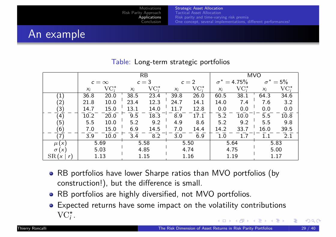
An example

Table: Long-term strategic portfolios

RB MVOc =∞ c = 3 c = 2 σ? = 4.75% σ? = 5%

xi VC?i xi VC?

i xi VC?i xi VC?

i xi VC?i

(1) 36.8 20.0 38.5 23.4 39.8 26.0 60.5 38.1 64.3 34.6(2) 21.8 10.0 23.4 12.3 24.7 14.1 14.0 7.4 7.6 3.2(3) 14.7 15.0 13.1 14.0 11.7 12.8 0.0 0.0 0.0 0.0(4) 10.2 20.0 9.5 18.3 8.9 17.1 5.2 10.0 5.5 10.8(5) 5.5 10.0 5.2 9.2 4.9 8.6 5.2 9.2 5.5 9.8(6) 7.0 15.0 6.9 14.5 7.0 14.4 14.2 33.7 16.0 39.5(7) 3.9 10.0 3.4 8.2 3.0 6.9 1.0 1.7 1.1 2.1µ (x) 5.69 5.58 5.50 5.64 5.83σ (x) 5.03 4.85 4.74 4.75 5.00

SR (x | r) 1.13 1.15 1.16 1.19 1.17

RB portfolios have lower Sharpe ratios than MVO portfolios (byconstruction!), but the difference is small.RB portfolios are highly diversified, not MVO portfolios.Expected returns have some impact on the volatility contributionsVC?i .





Efficient frontiers

RB frontier islower than MVfrontier (becauseof the logarithmicbarrier).c =∞ correspondsto the RB portfoliowith the highestvolatility (and thehighest expectedreturn).c → SR (x?|r)corresponds to theRB portfolio withthe highest Sharperatio.

Figure: Efficient frontier of SAA portfolios





Risk parity and absolute return funds

The risk/return profile of risk parity funds is similar to that of diversifiedfunds:

1 The drawdown is close to 20%;2 The Sharpe ratio is lower than 0.5.⇒ The (traditional) risk parity approach is not sufficient to build anabsolute return fund.

How to transform it to an absolute return strategy?1 By incorporating some views on economics and asset classes (global

macro fund, e.g. the All Weather fund of Bridgewater)2 By introducing trends and momentum patterns (long-only CTA)3 By defining a more dynamic allocation (BL, time-varying risk budgets,

etc.)





Calibrating the scaling factor

In a TAA model, the risk measure is no longer static:

Rt (xt) =−x>t µt + ct ·√x>t Σtxt

ct can not be constant because:1 the solution may not exist9.2 this rule is time-inconsistent (1Y 6= 1M):

Rt (xt ;c,h) = −h · x>t µt + c√h ·√

x>t Σtxt= h ·Rt

(xt ;c ′,1

)with c ′ = h−0.5c.

9There is no solution if c = Φ−1 (99%) and the maximum Sharpe ratio is 3.Thierry Roncalli The Risk Dimension of Asset Returns in Risk Parity Portfolios 32 / 40




An illustrationInvestment universe: MSCI World TR Net index, Citigroup WGBI AllMaturities indexEmpirical covariance matrix (260 days)Simple moving average based on the daily returns (260 days)Different rules:

ct = max(cES (99.9%) ,2.00 ·SR+

t)

(RP #1)ct = max

(cVaR (99%) ,1.10 ·SR+

t)

(RP #2)ct = 1.10 ·SR+

t ·1{

SR+t > 0

}+∞·1

{SR+

t ≤ 0}

(RP #3)

Table: Statistics of risk parity strategies

RP µ̂1Y σ̂1Y SR MDD γ1 γ2 τStatic #0 5.10 7.30 0.35 −21.39 0.07 2.68 0.30

#1 5.68 7.25 0.44 −18.06 0.10 2.48 1.14Active #2 6.58 7.80 0.52 −12.78 0.05 2.80 2.98

#3 7.41 8.00 0.61 −12.84 0.04 2.74 3.65Thierry Roncalli The Risk Dimension of Asset Returns in Risk Parity Portfolios 33 / 40




An illustration

Figure: Backtesting of RP strategies

The key issue is howto calibrate thescaling factor ct in aout-of-sampleframework /





Risk parity and time-varying risk premia

Optimality of the ERC portfolioThe ERC portfolio corresponds to the tangency portfolio if the Sharperatio is the same for all assets and the correlation is uniform.

The Sharpe ratio is constant if:the risk premia and the volatilities are constant;or the dynamic of the risk premia is the same as the dynamic of thevolatilities.

⇒ Risk premia are time-varying:General framework: Lucas (1976), Engle, Lilien and Robins (1987),Cochrane (2005).Stocks: Campbell and Shiller (1988), Lettau and Ludvigson (2001).Bonds: Cochrane and Piazzesi (2002), Dai and Singleton (2002),Diebold (2006).





Same weight compositions, but different economic regimes

Figure: Equivalent ERC compositions (static risk parity) Dec. 2002 –Mar. 2003 ≡ Jul.– Aug. 2010(26.5/73.5)Jul. 2000 ≡ Feb.– Mar. 2001 ≡Apr. – May 2002≡ Sep. 2003 ≡Dec. 2007 – Apr.2008 ≡ Feb. –May 2011(30/70)etc.





The rising interest rate challenge

30 years downward trend of interest rates

US 10-year sovereign interest rate: Peak 30/09/1981 15.80%Trough 25/07/2012 1.37%

⇒ A significant component of the good performance of (static) risk parityfunds.

The right benchmark is certainly not the 60/40 asset mix policy.What will be the performance of risk parity funds if the interest ratesrise?

Static risk parity vs active risk parity1994 scenario: fed fund = +300 bps / long rates = +250 bps⇒ static: /, active: ,1999 scenario: fed fund = +125 bps / long rates = +200 bps⇒ static: ,, active: ,





One concept, several implementations, differentperformances!

Choice of theinvestmentuniverseChoice of the riskbudgetsChoice of the TAAmodelChoice of theleverageimplementationChoice of therebalancingfrequencyetc.

Figure: Performance of RP funds in 2013

97.50

100.00

102.50

105.00

107.50

110.00

112.50

+ 9.97%

+ 1.44%

+ 13.79%

90.00

92.50

95.00

Dec-12 Jan-13 Feb-13 Mar-13 Apr-13 May-13 Jun-13 Jul-13 Aug-13 Sep-13 Oct-13 Nov-13

Lyxor ARMA 8 I EUR Invesco Balanced-Risk Alloc C AC Risk Parity 7 Fund EUR A Lyxor/SGI Harmonia Index

- 7.62%




Conclusion

Risk parity based on the volatility risk measure = not the right answerto build absolute return fund.

We propose a solution to incorporate discretionary views and trendsinto risk parity portfolios:

Expected returns = directional risks, and not performanceopportunities.It can be viewed as an active allocation strategy, but it remains a riskparity strategy.

But it is not a magic allocation method:

“It cannot free investors of their duty of making their ownchoices”.




ReferencesF. Barjou.Active Risk Parity Strategies are Up to the Interest Rate Challenge.Lyxor Research Paper, November 2013.

S. Maillard, T. Roncalli and J. Teïletche.The Properties of Equally Weighted Risk Contribution Portfolios.Journal of Portfolio Management, 36(4), 2010.

L. Martellini, V. Milhau.Towards Conditional Risk Parity – Improving Risk Budgeting Techniques inChanging Economic Environments.EDHEC Working Paper, March 2014.

T. Roncalli.Introduction to Risk Parity and Budgeting.Chapman & Hall, 410 pages, July 2013.

T. Roncalli.Introducing Expected Returns into Risk Parity Portfolios: A New Framework forTactical and Strategic Asset Allocation.SSRN, www.ssrn.com/abstract=2321309, July 2013.


www.ssrn.com/abstract=2321309

universityofparis6/paris7,april3,2014...

Documents