unleashing the full power of upf power states · unleashing the full power of upf power states...
TRANSCRIPT
Unleashing the Full Power of
UPF Power States
Erich Marschner Mentor Graphics Corporation
3919 River Walk
Ellicott City, MD 21042
USA
John Biggs ARM Ltd.
110 Fulbourn Road
Cambridge CB1 9NJ
UK
Keywords—low power design; low power verification; power modeling (key words)
Abstract—IEEE 1801 UPF [1] provides the ability to define power states of objects in a power-managed design. Power states drive analysis of isolation/level shifting requirements and can also be used for estimation of power dissipation. UPF power state definition is extremely flexible, but this comes at a cost: without a good methodology for defining power states, power intent can become complex and difficult to understand.
In this paper, we explain UPF power state definitions and the semantic issues that can arise from undisciplined usage. We present a taxonomy of power state definitions that differentiates fundamental, mutually exclusive, and non-mutually-exclusive power states. Using this taxonomy we define a methodology for power state definition and refinement that avoids semantic ambiguities and enables hierarchical composition of power intent as required by a successive refinement flow [2]. We relate this state taxonomy to the concepts of partially ordered sets and lattices [3] and to previous work such as Boole’s expansion theorem [4] and Harel’s Statecharts [5].
I. INTRODUCTION
The Unified Power Format (UPF) was developed to enable specification of active power management for RTL
designs, so that power management could be factored into early RTL verification and guide the implementation
process. Originally released as an Accellera standard in 2007, UPF development then moved to the IEEE; this led to
the release of IEEE Std 1801 UPF in 2009. More recently, updates to this standard were published in 2013 [1] and
2014.
Accellera UPF1 included support for defining the possible values of supply ports (“port states”) used to deliver
power to a system, together with “power state tables” (or PSTs) that defined legal combinations of port states. PST-
based analysis of the possible combinations of power supply values enabled UPF-supporting tools to determine
where isolation and level shifting would be required in a given design, and this is commonly used in tools today to
check that isolation and level shifting is actually inserted by the UPF power intent specification where it is required.
However, since power supplies typically originate off-chip and must be routed through the supply distribution
network to the power domains that comprise the system, Accellera UPF effectively required implementation of
power management in detail before verification could start. This tended to delay power aware verification until later
in the flow than necessary or require that verification be repeated later if earlier assumptions about implementation
details proved to be incorrect. Also, Accellera UPF had no way of specifying power management requirements for
IP components that might be used in a system. To address these issues, IEEE Std 1801 UPF added a number of new
features. Two of these are of particular relevance to this paper: supply sets, and power states.
A supply set represents the power provided to a power domain for a particular use, such as the primary supply of
the domain, an isolation supply, or a retention supply. Supply sets are an abstraction of connections to a power
distribution network, and they can be used to model incoming power to the domain before the supply distribution
network has been defined. Supply sets for a given power domain are defined along with the power domain. They
can also be defined as separate objects via the create_supply_set command.
A power state represents a particular mode of operation of supply set or a power domain. For a supply set, a
given power state indicates whether and how it is providing power to a power domain or related power management
cell. For a power domain, a power state indicates the current operational mode of that domain, and as a
consequence, whether or how the power domain is consuming power. Power states are defined with the
add_power_state command.
1 Also known as UPF 1.0.

The add_power_state command is an extremely flexible and powerful command that enables the user to construct
very complex power state definitions sufficient to model any possible situation. However, that flexibility and
power, if used indiscriminately, can result in power state definitions that are difficult to understand, difficult to
debug, and even difficult for tools to analyze. To avoid these potential problems, it is important to understand what
power states represent, how they can be defined in an orderly and methodical fashion to ensure maximum clarity,
and how they can be organized to most effectively support verification and analysis by tools.
A. The add_power_state Command
The UPF add_power_state command defines power states of a supply set or a power domain.
Any number of power states can be defined for a given object. Power states of a given object are defined in terms
of the states of other objects that either comprise the given object or are contained in or below the HDL scope in
which the given object is defined.
Each power state is defined in terms of a supply expression, a logic expression, or both. A supply expression is
used only for supply set power states; it refers to supply states of the functions of that supply set. A logic expression
can be used in the definition of power states for either supply sets or power domains. It can refer to control
conditions, clock frequencies, and power states of the domain’s supply sets.
Each power state can be defined as either legal or illegal. If unspecified, the default is legal. A supply set power
state can also specify a simstate, which defines how logic powered by this supply set will behave in simulation when
in this power state. Simstate values range from NORMAL to CORRUPT, with intermediate values indicating
successively more sensitivity to changes that could cause corruption.
An initial power state definition can be refined later by repeating the command with the -update option.
Command refinement can extend an existing state definition - for example, to add a logic expression. It can also
extend an existing state’s supply expression or logic expression by ANDing the original with a new term.
#---------------------------------------------------------------
# Example Power State Definitions
# Adapted from examples in IEEE Std 1801-2013, clause 6.4, pg 57
#---------------------------------------------------------------
# Power states for the primary supply set of power domain PDA
add_power_state PDA.primary –supply \ -state {ON –simstate NORMAL \ –logic_expr {SW_ON} \ -supply_expr { power == {FULL_ON 0.8} && \ ground == {FULL_ON 0.0} } } \ -state {OFF –simstate CORRUPT \ –logic_expr {!SW_ON} \ -supply_expr { power == OFF || \ ground == OFF } } # Another power state for the primary supply set of power domain PDA
add_power_state PDA.primary –supply –update \ -state {SLOW –simstate CORRUPT_STATE_ON_CHANGE \ –logic_expr {SW_ON && interval(clk posedge negedge)>= 100ns} \ -supply_expr { power == {FULL_ON 0.8} && \ ground == {FULL_ON 0.0} } } # Updating the previous state definitions to include nwell specifications add_power_state PDA.primary –supply –update \ -state {ON –supply_expr { nwell == {FULL_ON 0.8} } } \ -state {SLOW –supply_expr { nwell == {FULL_ON 1.0} } } # Declaring that there are no more legal power states of PDA.primary add_power_state PDA.primary –supply –update –complete # Power states of power domain PDA based on its primary supply and a control input add_power_state PDA –domain \ -state {RUN –logic_expr { primary == ON && !sleep } } \

-state {SLEEP -logic_expr { primary == ON && sleep } } \ -state {SHUTDOWN –logic_expr { primary == OFF } } # Power states of power domain PDTOP based on the power states of domains PDA, PDB add_power_state PDTOP –domain \ -state {S1 –logic_expr { PDA == RUN && PDB == RUN } } \ -state {S2 –logic_expr { PDA == SLEEP || PDB == SLEEP } } \ -state {S3 –logic_expr { PDA != RUN && PDB != SHUTDOWN } }
B. The Power of add_power_state
The add_power_state command is very powerful in part because the supply and logic expressions used to define
power states allow for general Boolean expressions. As the above example code illustrates, these expressions
include support for the following special subexpression forms:
- interval (signal name [, edge1 [, edge2]])
- for detecting clock frequencies
- supply == {supply net state [voltage1 [voltage2]]}
- for detecting a supply port/net or supply set function’s value
- supply set == power state
- for detecting the state of a supply set that affects another object’s power state
- power domain == power state
- for detecting the state of a power domain that affects another object’s power state
Since power states are defined with Boolean expressions, they are essentially predicates. When a given power
state’s defining expressions are True, that power state is active. As a consequence of this definitional approach,
more than one power state can be active at a given time. This allows definition of non-mutually-exclusive power
states as well as mutually-exclusive power states.
II. ISSUES WITH ADD_POWER_STATE
A. Non-Mutually-Exclusive States can be a Problem
For some applications, non-mutually exclusive states are quite useful. In particular, they can be used to express
abstraction, in which a more general state represents a set of more specific states, and therefore the more general
state overlaps with (is not mutually exclusive with respect to) each of the more specific states. For example, an
abstract power state ON could be defined as an abstraction of the set of more specific power states {NORMAL,
ECO, TURBO}.
For other applications, non-mutually-exclusive states are often problematic. For example, such states make
reasoning about state transitions more difficult. Is it possible to transition from a more specific state to a more
general state? Or vice versa? For some applications, mutually exclusive states are absolutely required, such as
when attempting to model power consumption of a component.
When power states are defined with general Boolean expressions, determining whether two power states are
mutually exclusive can be challenging, both for users and for tools. In general this requires support for Boolean
expression analysis, which is typically available in some tools but not others.
B. Semantics of –update Are Not Sufficient
UPF is intended to support successive refinement of power intent [1], in which information is specified
incrementally as it becomes available. In a successive refinement flow, usage constraints are specified for system
components, logical configuration information is then specified when components are integrated into a system, and
physical implementation details are then specified in order to drive the implementation process.
Part of successive refinement is refinement of power state definitions. Fundamental power states for components
can be specified along with constraints. These states can be refined further when the system is configured, to reflect
power management decisions. These states can be further refined with technology-specific information when
implementation details are provided.
Refinement creates a more specific state derived from a previously defined power state. This new state is
necessarily non-mutually-exclusive with respect to the previously defined state. The add_power_state command
does support refinement of a sort using its -update option. However, such refinement is strictly linear. To be truly
useful, a successive refinement methodology requires support for branching refinement, in which a given abstract
state can be refined multiple times to produce independent refined states, each of which is non-mutually-exclusive
with respect to the original state.
C. Updating a Power State with -update
Another problem with add_power_state -update is that it changes the definition of the original state. Since the
definition of one power state may depend upon another object being in a particular power state, a change to the
definition of a power state of one object may affect the definition of a power state of another object. The “update-
in-place” semantics of add_power_state -update can therefore have unexpected effects throughout the set of power
state definitions for a system.
D. How Power State Definitions Should Work
Ideally, it should be possible to do the following
• define fundamental power states as mutually exclusive states
• refine existing power states multiple times to create new, more specific (and mutually exclusive) variants
• refer to a power state without any risk of its definition being undermined by later changes
In particular, power state refinement should
• enable identification of a unique current power state, and
• preserve the ability to detect illegal states and illegal transitions
Also, it should be easy to determine whether two power states are expected to be mutually exclusive or not, both
for tools and for users.
III. POWER STATE DEFINITION AND REFINEMENT CONCEPTS
A. What Exactly is a Power State?
Any object consists of a set of items that characterize its functional state. For example, a supply set’s state is
characterized by the states of its supply set functions; a power domain’s state is characterized by the states of its
supply sets; an IP block’s state is characterized by the states of its constituent elements (power domains and macro
instances). The set of all possible combinations of values of these characteristic items is the set containing all
possible functional states of the object. This set of possible value combinations defines the functional state space of
the object.
A power state represents a subset of this set of all possible functional states of an object, or equivalently, a region
within the functional state space of the object. The defining expression of a power state evaluates to True for every
value combination in this subset and evaluates to False for every value combination outside this subset.
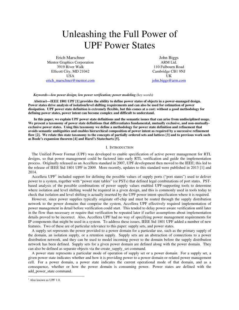
Figure 1 illustrates this concept. The state of an object O is characterized by the values of its constituent
elements, A, B, and C, which are Boolean-valued signals, so there are 23 = 8 possible functional states of object O.
For this object, three power states have been defined: S1, S2, and S3, each with its respective defining expression
over the characteristic elements of O. Of these elements, C is a don’t care in all three power states; the defining
expressions only refer to A and B.
A B C
0 0 0
0 0 1
0 1 0
0 1 1
1 0 0
1 0 1
1 1 0
1 1 1
A==0
&&
B==0
A != B
A==1
&&
B==1
don’t
cares
S1
S2
S3
Figure 1. Power State Definition
Why do we use the term “power state” for these subsets of functional states? There are two reasons. For some
objects, the characteristic elements are supply sources such as power and ground rails, and therefore their
“functional states” actually represent their ability to provide power to devices to which they are connected. For
other objects, their functional states indicate which of their component elements are actively operating and therefore
which logic elements will consume power in that functional mode. While these are slight different concepts, it is
convenient to lump both into the category of “power state”.
B. What Exactly is Power State Refinement?
Refinement of a power state amounts to subsetting. Refining a given power state involves definition of a new
power state characterized by a more restricted subset of the functional states of the given power state. A refined
power state is therefore always contained within the functional state space of the original, more abstract power state.
Refinement (i.e., restriction) is accomplished by imposing additional requirements that must be satisfied by the set
of characteristic item values that define the more abstract power state. This amounts to extending the defining
expression of the more abstract power state with another condition. For example, if the more abstract power state’s
defining expression is {C1}, then a refinement of that power state might have the defining expression {C1 && C2},
where C2 is the additional condition that must be satisfied by the values of that object’s characteristic elements for
that object to be in the more refined state.
This is similar to how -update works, but with -update the original definition is changed rather than creating a new
definition. Use of –update amounts to “refinement in place”, in that the original definition is modified in the
process.
#---------------------------------------------------------------
# Power state “refinement in place” using -update
#---------------------------------------------------------------
add_power_state PDA –domain \ -state {A1 \ –logic_expr {C1} } add_power_state PDTOP –domain \ -state {TOP1 \ –logic_expr {PDA == A1 && C2} } # The above is equivalent to # add_power_state PDTOP –domain \ # -state {TOP1 \ # –logic_expr {C1 && C2} } add_power_state PDA –domain –update \
-state {A1 \ –logic_expr {!C2} } # The above is equivalent to # add_power_state PDA –domain –update \ # -state {A1 \ # –logic_expr {C1 && !C2} } # And it causes a ripple effect on PDTOP # add_power_state PDTOP –domain \ # -state {TOP1 \ # –logic_expr {C1 && C2 && !C2} } ;# <= contradiction
C. Branching Refinement
An alternative to “refinement in place” is “refinement by derivation”. This approach involves defining a new
power state (with a new name), based on the original power state. Such refinement can be done any number of
times without modifying the original power state definition. Each refinement produces a new power state that is
non-mutually-exclusive with the original abstract state. This non-mutual-exclusion is useful for representing
abstraction and for enabling top-down design. However, we will impose a requirement that all refinements of the
same parent object must be mutually exclusive.
“Refinement by derivation” preserves the original power state definition and thus avoids unexpected semantic
changes in other commands that refer to that original power state. This kind of refinement results in an
abstraction/refinement hierarchy in which more abstract states are refined to create more specific states.
This method also enables orthogonal definition of mutually-exclusive and non-mutually-exclusive states: sibling
states (refined from the same parent state) must be mutually-exclusive, whereas states related by refinement (on the
same path from the root to a leaf of the refinement hierarchy) will be non-mutually-exclusive.
#---------------------------------------------------------------
# Power state “refinement by derivation”
#---------------------------------------------------------------
add_power_state PDA –domain \ -state {A1 \ –logic_expr {C1} } add_power_state PDTOP –domain \ -state {TOP1 \ –logic_expr {PDA == A1 && C2} } # This is equivalent to # add_power_state PDTOP –domain \ # -state {TOP1 \ # –logic_expr {C1 && C2} } # Refining state A1 by adding another condition to its logic expression {C1} add_power_state PDA –domain –update \ -state {A1R \ –logic_expr {C1 && !C2} } # Refined State A1R can now be used instead of A1 where required # The definition of state TOP1 of PDTOP remains unaffected
D. Definite, Indefinite, and Deferred Power States
Given the view of refinement as subsetting the functional state space of an object, refinement is well-defined
when the defining expression of a power state is limited to equality and conjunction. Such a defining expression
effectively specifies a particular binding of values to the variables that characterize the state (the care set). When a
power state R is defined as a refinement of a more abstract state A, the defining expression of R will effectively
include the defining expression of A conjoined with additional conditions that restrict the state space to R.
To capture this idea, we introduce the concept of a “definite power state”. A definite power state of an object OBJ
is a state whose defining expression is a conjunction of terms of the form <obj>==<state>, where <obj> is a
characteristic element of object OBJ, and <state> is a definite state of that element. A term in the defining
expression of a definite power state can also be a Boolean expression that refers only to control conditions in the
design, including use of the UPF interval function. Such terms terminate the recursion in the first part of the
definition.
Refinement is not as well-defined for operators other than equality and conjunction. In particular, use of
disjunction or negation in the defining expression of a power state implies potentially multiple values for the objects
whose values characterize that state. To reflect this, we introduce the concept of an “indefinite power state”. An
indefinite power state is one whose defining expression is not of the form required for a definite state or contains a
term that refers to an indefinite state of another object.
In some cases, the defining expression of a power state is not known when it is first defined, typically because it
depends upon information that is not yet available. For example, technology-specific or implementation-specific
information such as whether a given supply will be switched using header switches (for the power rail) or footer
switches (for the ground rail) may not be available when the OFF state of a supply set is defined. In such cases, the
defining expression may be left unspecified, to be completed later. We refer to such a case as a “deferred power
state”. For convenience, we will assume that a deferred power state will eventually become a definite power state
when its defining expression is known. This allows deferred power states to be referred to in the defining
expression of another definite power state.
IV. A METHODICAL APPROACH TO DEFINING POWER STATES
A. A New Model for Power State Refinement
Given the above-mentioned concepts, we can now present a coherent model for power state definition and
refinement:
• Fundamental power states are those that do not refer to any other power state of the same object. They can
be either definite, indefinite, or deferred states.
• For any object, there exists a predefined power state UNDEFINED that initially represents the set of all
possible states of an object. Fundamental power states are carved out of the UNDEFINED state using
mutually-exclusive defining expressions. The UNDEFINED state therefore ultimately represents all
states that are not defined as fundamental power states. The UNDEFINED power state’s defining
expression is therefore essentially the condition “no fundamental state is active”.
• Definite states can be refined by derivation to create a set of mutually-exclusive substates or refinements.
Indefinite states cannot be refined. Deferred states can be updated later (using refinement in place) to
complete their definition; such updates must result in definite states.
• If state R is a refinement of state A, then A is an abstraction of R, and A, R are related by refinement.
• An ERROR state is predefined for any object. This ERROR state becomes active if any two states not
related by refinement are active at the same time.
This refinement methodology encourages the definition of mutually exclusive power states, but there is still a
need to ensure that states are mutually exclusive. For simulation this implies a dynamic (runtime) check; for static
verification tools, this implies a need for Boolean analysis.
B. Active and Current Power States
Since states that are related by refinement are not mutually exclusive, it is possible to have multiple states active
at the same time. For situations where it is important to identify a single unique state for an object, a precedence
rule is introduced.
A state is active if its defining expression is true. If two states that are related by refinement are active at the same
time, then the most refined state shall take precedence. This is reflected in the following algorithm for determining
the current power state:
If only one power state is active,
that state is the current power state;
Else if more than one definite power state is active, and all active states are related by refinement,
then the most refined state is the current power state;
Else ERROR is the current power state
Note that the UNDEFINED state will be active if no other (fundamental or refined) power state is active, so the
first part of this algorithm may result in identifying the UNDEFINED state and the current power state.
C. Implementing this Model with add_power_state
This approach to power state definition and refinement can be implemented today using the current2 features of
the add_power_state command in a particular manner. The following set of guidelines explain how to accomplish
this.
For any given object O, define the power states of that object as follows:
1. Define the fundamental power states of the object, taking care to ensure that the defining expressions of
the fundamental power states are mutually exclusive. Where possible, define definite power states or
deferred power states rather than indefinite power states.
2. When refinement of an existing state becomes necessary, use refinement by derivation. Instead of
copying the original state’s supply or logic expressions, refer to the existing state by name in the logic
expression. For example, to refine an existing state S of object O, define a new state SR whose logic
expression includes the term (O==S). This will have the same effect as copying the defining expression
of state S into the definition of state SR.
3. When refining the same existing state more than once, ensure that each refinement’s defining expression
is mutually exclusive with respect to the others’.
4. Define an UNDEFINED state with the logic expression (O != FS1 && O != FS2 && … O != FSn), where
FSk (k=1..n) represent the fundamental states of O. For example, for a supply set SS with fundamental
states ON and OFF, define state UNDEFINED with the logic expression (SS != ON && SS != OFF).
5. Define an ERROR state with a logic expression that will be True if any two fundamental states of O are
active at the same time. For example, for a supply set SS with fundamental states ON and OFF, define
state ERROR with the logic expression (SS==ON && SS==OFF).
6. If object O is a supply set object, then
• for the UNDEFINED state, do not specify a simstate.
• for any refinement R of a power state A, ensure that the simstate of R is at least as conservative as
that of A (where NORMAL is least conservative, CORRUPT is most conservative).
• for the ERROR state, specify a simstate of CORRUPT.
The above guidelines ensure that the power states of an object are defined in a consistent, hierarchical manner,
with mutually-exclusive states in each layer of the hierarchy, with non-mutually-exclusive states representing
abstraction/refinement along any path down the hierarchy, and with an UNDEFINED state and an ERROR state to
represent situations in which no fundamental state or more than one fundamental state is active at the same time.
The last guideline regarding simstates ensures that the existing simstate precedence rules in UPF 2.x will effectively
give the same result as the precedence rule given above for determining the current power state.
D. Example Application of these Guidelines
To illustrate the use of the above guidelines in a practical example, we present power state definitions for a power
domain PD and its primary supply set PD.primary.
The fundamental power states of a supply set generally include an ON state and an OFF state. The ON state
requires that both power and ground supplies are in their FULL_ON state; voltages for those supplies may be
technology-dependent and can be added later (using –update). The OFF state typically implies that either the power
or ground rail is switched. This is implementation-dependent and therefore may need to be added later (with –
update); if so, the definition of OFF can be left as a deferred power state. So the initial set of power states for supply
set PD.primary would be as follows:
#---------------------------------------------------------------
# Power states for supply set PD.primary
#---------------------------------------------------------------
add_power_state PD.primary -supply \ -state {UNDEFINED \ -logic_expr {PD.primary != ON && PD.primary != OFF} } \
2 UPF 2.0 (1801-2009) or 2.1 (1801-2013) or 2.2 (1801-2014)

-state {ON –simstate NORMAL \ –supply_expr {power == FULL_ON && ground == FULL_ON} } \ -state {OFF –simstate CORRUPT \ -state {ERROR –simstate CORRUPT \ -logic_expr {PD.primary == ON && PD.primary == OFF} }
This set of power state definitions for a supply set is sufficient to enable definition of the fundamental power
states of a power domain. In the simplest case, we might define the fundamental power states of domain PD as
follows:
#---------------------------------------------------------------
# Power states for power domain PD
#---------------------------------------------------------------
add_power_state PD -domain \ -state {UNDEFINED \ -logic_expr {PD != UP && PD != DOWN} } \ -state {UP \ –logic_expr {primary == ON} } \ -state {DOWN \ –logic_expr {primary == OFF} } \ -state {ERROR \ -logic_expr {PD == UP && PD == DOWN} }
If state retention is required for power domain PD, we can add additional retention states through refinement of
the existing states. There are various ways to implement state retention. Depending the style of state retention
adopted in a given design, different refinements of the fundamental states described above may be appropriate.
For example, state retention can be implemented by using retention registers, which may require a retention
supply. Suppose power domain PD has another supply, PD.retention, with the same set of power states defined for
it as we defined above for PD.primary. In that case, we might add a retention state to the set of power states defined
for domain PD, as follows:
#---------------------------------------------------------------
# Retention power state for power domain PD
#---------------------------------------------------------------
add_power_state PD -domain –update \ -state {RET \ -logic_expr {PD == DOWN && PD.retention == ON} }
This refines the UP state of power domain PD by conjoining the condition PD.retention==ON with the original
condition PD.primary==OFF, given by the definition of power state DOWN. Note that if PD is in the RET state, it
will also be in the DOWN state, because the defining expression for the RET state contains the defining expression
for the DOWN state, and therefore the state space represented by the DOWN state contains the state space
represented by the RET state. In that case, the precedence rule given above would identify the RET state as the
current power state.
Another way of modeling state retention might be to put the PD.primary supply into a low voltage or bias state in
which the logic in the domain will maintain its state provided that its inputs do not change. This can be modeled by
refining the PD.primary supply set’s ON state to create a retention state, rather than refining the power states of
domain PD. This could be done as follows:
#---------------------------------------------------------------
# Retention power state for supply set PD.primary
#---------------------------------------------------------------
add_power_state PD.primary -supply –update \ -state {RET –simstate CORRUPT_ON_CHANGE \ -logic_expr {PD.primary == ON && sleep} }
where ‘sleep’ is a control signal that causes PD.primary to go into a low voltage or bias state. Note that in this
case, since RET is a supply set power state, we include simstate CORRUPT_ON_CHANGE to ensure that the
domain logic will be corrupted if its inputs change while in this state. Since CORRUPT_ON_CHANGE is more
conservative than the NORMAL simstate of power state ON, the existing UPF 2.x simstate precedence rules would
apply the CORRUPT_ON_CHANGE simstate when the supply set is in both the ON and RET power states at the
same time.
Another application of power state refinement would be to define performance states. For example, we might
define the following power states to represent various levels of performance:
#---------------------------------------------------------------
# Low, Med, and High performance power states for supply set PD.primary
#---------------------------------------------------------------
add_power_state PD.primary -supply –update \ -state {LOW –simstate NORMAL \ -logic_expr {PD.primary == ON && perfmode==2’b10} } \ -state {MED –simstate NORMAL \ -logic_expr {PD.primary == ON && perfmode==2’b00} } \ -state {HIGH –simstate NORMAL \ -logic_expr {PD.primary == ON && perfmode==2’b01} } \
where ‘perfmode’ is a control signal that ultimately will control the voltage level on PD.primary to enable support
for the selected level of performance. In each case, there may also be a maximum clock speed allowed for that state.
This could be captured using the UPF ‘interval’ function, either in the above refinements of ON state of supply set
PD.primary, or in corresponding refinements of the UP state of power domain PD, such as the following:
#---------------------------------------------------------------
# Slow, Norm, and Fast performance power states for power domain PD
#---------------------------------------------------------------
add_power_state PD -domain –update \ -state {SLOW \ -logic_expr {PD == UP && PD.primary == LOW && interval(clk) >= 1ns} } \ -state {NORM \ -logic_expr {PD == UP && PD.primary == MED && interval(clk) >= 500ps} } \ -state {FAST \ -logic_expr {PD == UP && PD.primary == HIGH && interval(clk) >= 333ps} } \
These definitions specify that the clock frequency (indicated by the delay between posedge events, which is the
default for the interval function) is no faster than 1GHz in the SLOW state, 2GHz in the NORM state, and 3GHz in
the FAST state. Once again, if one of these performance states of PD is active, then power state UP of PD will also
be active, but the precedence rule for power states will identify the most refined state as the current power state.
Note that it would not be possible to remove the references to PD.primary in the above definitions. If the
references to PD.primary == LOW, MED, or HIGH were removed from these definitions, then these states would no
longer be mutually exclusive with respect to each other, since if the term (interval(clk) >= 1ns) were true, then both
of the other interval functions would necessarily also be true. This is an illustration of the need for care in defining
refinements of a given state, to ensure that all refinements of the same state are mutually exclusive with respect to
each other.
V. RELATED WORK
The power state definition model described has characteristics that are similar to, and in at least one case inspired
by, other systems of state definition and organization. In this section we compare and contrast the UPF power state
definition and refinement model with those other systems.
A. Partially Ordered Sets and Lattices
When the power state definitions described in section IV above are followed, the resulting set of power states
represents an abstraction/refinement hierarchy. This power state hierarchy is a partially ordered set [3], in which
the refinement process defines a partial order over the power states. The refinement relation defines a partial order
primarily because the refinement relation is transitive (if C refines B, and B refines A, then C refines A). This
relation is also antisymmetric (although vacuously, since we disallow cycles in the refinement hierarchy and
therefore there cannot exist two states that are refinements of each other) and reflexive (a state A can be viewed as
either itself or as a refinement itself involving the additional condition ‘True’).
When such a power state hierarchy is viewed as a partially ordered set, any path from a fundamental state to its
most refined state is a chain, since the set of states along that path is given a total order by the refinement relation.
Similarly, the set of fundamental states (and the set of refinements of any given state) is an antichain, since states at
any given level of the hierarchy are not related by refinement and therefore are unordered by the refinement relation.
The power states UNDEFINED and ERROR are the minimal and maximal elements, respectively, of this partially
ordered set.
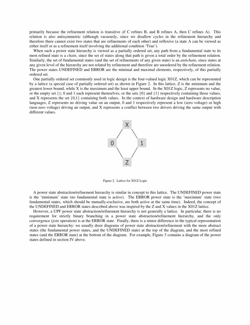
One partially ordered set commonly used in logic design is the four-valued logic X01Z, which can be represented
by a lattice (a special case of partially ordered set) as shown in Figure 2. In this lattice, Z is the minimum and the
greatest lower bound, while X is the maximum and the least upper bound. In the X01Z logic, Z represents no value,
or the empty set {}; 0 and 1 each represent themselves, or the sets {0} and {1} respectively containing those values,
and X represents the set {0,1} containing both values. In the context of hardware design and hardware description
languages, Z represents no driving value on an output, 0 and 1 respectively represent a low (zero voltage) or high
(non-zero voltage) driving an output, and X represents a conflict between two drivers driving the same output with
different values.
X
Z
0 1
Figure 2. Lattice for X01Z Logic
A power state abstraction/refinement hierarchy is similar in concept to this lattice. The UNDEFINED power state
is the ‘minimum’ state (no fundamental state is active). The ERROR power state is the ‘maximum’ state (two
fundamental states, which should be mutually-exclusive, are both active at the same time). Indeed, the concept of
the UNDEFINED and ERROR states described above was inspired by the Z and X values in the X01Z lattice.
However, a UPF power state abstraction/refinement hierarchy is not generally a lattice. In particular, there is no
requirement for strictly binary branching in a power state abstraction/refinement hierarchy, and the only
convergence (join operation) is at the ERROR state. Finally, there is a minor difference in the typical representation
of a power state hierarchy: we usually draw diagrams of power state abstraction/refinement with the more abstract
states (the fundamental power states, and the UNDEFINED state) at the top of the diagram, and the most refined
states (and the ERROR state) at the bottom of the diagram. For example, Figure 3 contains a diagram of the power
states defined in section IV above.
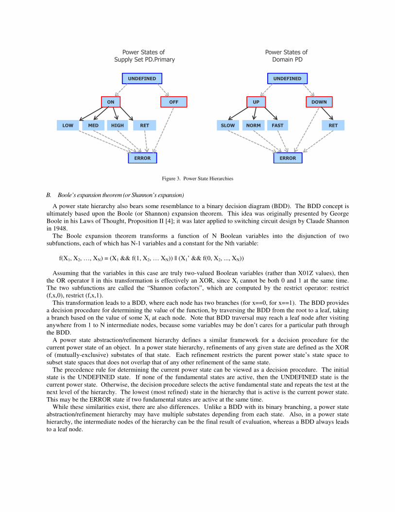
UNDEFINED
ERROR
ON OFF
MED HIGH RETLOW
UNDEFINED
ERROR
UP DOWN
NORM FAST RETSLOW
Power States of Supply Set PD.Primary
Power States of Domain PD
Figure 3. Power State Hierarchies
B. Boole’s expansion theorem (or Shannon’s expansion)
A power state hierarchy also bears some resemblance to a binary decision diagram (BDD). The BDD concept is
ultimately based upon the Boole (or Shannon) expansion theorem. This idea was originally presented by George
Boole in his Laws of Thought, Proposition II [4]; it was later applied to switching circuit design by Claude Shannon
in 1948.
The Boole expansion theorem transforms a function of N Boolean variables into the disjunction of two
subfunctions, each of which has N-1 variables and a constant for the Nth variable:
f(X1, X2, …, XN) = (X1 && f(1, X2, … XN)) || (X1’ && f(0, X2, ..., XN))
Assuming that the variables in this case are truly two-valued Boolean variables (rather than X01Z values), then
the OR operator || in this transformation is effectively an XOR, since Xi cannot be both 0 and 1 at the same time.
The two subfunctions are called the “Shannon cofactors”, which are computed by the restrict operator: restrict
(f,x,0), restrict (f,x,1).
This transformation leads to a BDD, where each node has two branches (for x==0, for x==1). The BDD provides
a decision procedure for determining the value of the function, by traversing the BDD from the root to a leaf, taking
a branch based on the value of some Xi at each node. Note that BDD traversal may reach a leaf node after visiting
anywhere from 1 to N intermediate nodes, because some variables may be don’t cares for a particular path through
the BDD.
A power state abstraction/refinement hierarchy defines a similar framework for a decision procedure for the
current power state of an object. In a power state hierarchy, refinements of any given state are defined as the XOR
of (mutually-exclusive) substates of that state. Each refinement restricts the parent power state’s state space to
subset state spaces that does not overlap that of any other refinement of the same state.
The precedence rule for determining the current power state can be viewed as a decision procedure. The initial
state is the UNDEFINED state. If none of the fundamental states are active, then the UNDEFINED state is the
current power state. Otherwise, the decision procedure selects the active fundamental state and repeats the test at the
next level of the hierarchy. The lowest (most refined) state in the hierarchy that is active is the current power state.
This may be the ERROR state if two fundamental states are active at the same time.
While these similarities exist, there are also differences. Unlike a BDD with its binary branching, a power state
abstraction/refinement hierarchy may have multiple substates depending from each state. Also, in a power state
hierarchy, the intermediate nodes of the hierarchy can be the final result of evaluation, whereas a BDD always leads
to a leaf node.

C. Harel’s Statecharts
Statecharts [5] are diagrams representing hierarchical state machines that enable graphical modeling of state
abstraction/refinement and concurrent operation communication among system elements. Statecharts were
introduced for modeling reactive systems, which are difficult to describe with flat finite state machines because the
concurrent operation of their subcomponents lead to exponential state explosion when the state space is flattened.
Key concepts supported by Statecharts include clustering of states into superstates, refinement of states, the ability
to model independent or orthogonal sets of states, and the ability to model abstract or generalized state transitions.
These concepts closely parallel the concepts described above for UPF power states.
Clustering of two states represents the XOR of those states, which implies that the cluster is an abstraction of the
states in the cluster. This operation can be performed bottom-up (grouping existing states into a superstate) or top-
down (partitioning an existing state into substates). The latter corresponds to refinement of a power state to create a
set of mutually-exclusive new states.
Statecharts also support AND decomposition of a state as a conjunction of substates. This represents concurrent
operation of subordinate components and implies “orthogonal product” states of the collection of referenced
components. It can be used to represent either synchronization of those components (when an event causes entry
into the superstate) or independent operation (when an event causes only one subordinate component to change
state). The AND decomposition is analogous to the concept of a Definite State in UPF, in which a given power state
has a defining expression that is a conjunction of terms, each of which test for the state of another object. However,
in UPF it is an error for a given object to be in multiple states at the same time, so in UPF the AND decomposition
typically refers to states of other objects, not states of the same object.
Statecharts can also express non-mutually-exclusive OR decomposition, which is analogous to the Indefinite
States of UPF. As in UPF, such states can lead to semantic issues (including non-determinism), but nonetheless they
are necessary or convenient in some situations.
Statecharts involve a number of control mechanisms for determining which substate is entered when an aggregate
state is entered. Not all of these capabilities are present in UPF, although the ability to refer to control expressions
in the defining expression of a power state may enable emulation of some of these features.
Statecharts exhibit an implicit assumption of completeness—that all possible superstates and substates are
defined. UPF does not make this assumption, in part to allow for incremental evolution of the UPF power intent
specification over the lifetime of a project, and in part to avoid having to define transient intermediate states that
may occur in the design between defined states. This is illustrated by the explicit modeling of the UNDEFINED
state in UPF. It is also reflected in the definition of active and current power states: the definition of active state
treats a given state as a true abstraction of all of its refinements; the definition of current state treats a given state as
representing that abstraction minus its refinements. This could also be viewed as the notion that any given UPF
power state has an implicit default substate which is the given state excluding all other substates.
Statecharts provide a vehicle for presenting both states and transitions in an integrated, graphical manner. In this
paper we have largely focused on UPF power states, but many of the same issues regarding transitions to or from
abstract superstates that are addressed by Statecharts are also relevant to UPF.
VI. FUTURE WORK
Although the approach to power state definition and refinement described above can be implemented in UPF 2.x,
the UPF specification could be enhanced to support and encourage this approach more effectively. To that end, a
number of changes are planned for the upcoming UPF 3.0 standard.
First, the concepts described above will be explained in the specification. In particular, these include the concepts
of Definite, Deferred, and Indefinite power states, and the concept of Refinement by Derivation and how it differs
from Refinement in Place with –update. The concepts of state abstraction and refinement, the refinement relation,
and fundamental power states will also be explained.
In addition, a syntax extension will enable power state refinement without using the logic expression. This is
needed because in some situations such as early system level power analysis, the power state refinement hierarchy
needs to be defined before the control conditions and dependencies upon other objects’ states are known. This
syntax extension will allow dotted names to be used for power states, with the implication that the full dotted name
is a refinement of a power state whose name is the prefix of the dotted name. For example, power state name
ON.TURBO would imply that this state is a refinement of power state ON.
Various semantic extensions and modifications will also come into play. This includes addition of the predefined
power states UNDEFINED and ERROR, as well as the supply set power states OFF and ON, and possibly

predefined power states for domains as well (for example, UP and DOWN). The semantics of the add_power_state
–complete option will also be revised slightly to allow for refinement of existing states while still prohibiting
creation of new states. The precedence rules for determining the current power state will be added, and these will
replace the existing precedence rules for simstate application. Finally, the effect of these changes will be applied to
clarify the semantics of the describe_state_transition command.
VII. SUMMARY
The UPF add_power_state command is a very flexible and powerful way of modeling the power states of an
object within a system. That flexibility and power, if used without discipline, can result in potentially complex and
difficult to understand power intent specifications.
In this paper we have described the types of problems that can result, especially those related to the conflicting
requirements for both mutually-exclusive and non-mutually-exclusive power states. We have presented a new
model for power state refinement, refinement by derivation, that supports a much more coherent approach to
definition of a hierarchy of power states through refinement. We have shown how this model can be used to define
the fundamental power states of both supply sets and domains, as well as refinements of those fundamental power
states as appropriate for a particular power management configuration.
We have also shown how this approach relates to previous work in the area of defining hierarchical power states.
Finally, we have outlined the enhancements planned for UPF 3.0 to more directly support and encourage the use of
this new model for power state definition and refinement.
REFERENCES
[1] IEEE Standard for Design and Verification of Low-Power Integrated Circuits, IEEE Std 1801, May 2013. [2] A. Khan, E. Quigley, J. Biggs, E. Marschner, Successive Refinement: A Methodology for Incremental Specification of Power Intent. Design
and Verification Conference (DVCon) 2015. [3] C. L. Liu. Elements of Discrete Mathematics. New York: McGraw-Hill, 1977, pp. 57-68. [4] G. Boole. An Investigation into the Laws of Thought. New York: Dover, 1958, pp. 73-78. (Original New York: Macmillan, 1854) [5] D. Harel. “Statecharts: A Visual Formalism for Complex Systems”. Science of Computer Programming, vol. 8, pp. 231-274, 1987.
DVCon US 2015