arX

iv:1

605.

0680

8v2

[ast

ro-p

h.H

E]

24 M

ay 2

016

Astronomy& Astrophysicsmanuscript no. m_LMC_x-3 c©ESO 2018September 26, 2018

Unraveling the Formation History of the Black Hole X-ray BinaryLMC X-3 from ZAMS to Present

Mads Sørensen1, Tassos Fragos1, James F. Steiner2, Vallia Antoniou3, Georges Meynet1, and Fani Dosopoulou4

1 Observatoir de Genéve, University of Geneva, Route de Sauverny, 1290 Versoix, Switzerland2 MIT Kavli Institute for Astrophysics and Space Research, Cambridge, MA 02139, USA3 Harvard-Smithsonian Center for Astrophysics, 60 Garden Street, Cambridge, MA 02138, USA4 Center for Interdisciplinary Exploration and Research in Astrophysics (CIERA) and Department of Physics and Astrophysics,

Northwestern University, Evanston, IL 60208

September 26, 2018

ABSTRACT

Aims. We have endeavoured to understand the formation and evolution of the black hole (BH) X-ray binary LMC X-3. We estimatethe properties of the system at 4 evolutionary stages: 1) at the Zero Age Main Sequence (ZAMS), 2) just prior to the supernova (SN)explosion of the primary, 3) just after the SN, and 4) at the moment of RLO onset.Methods. We use a hybrid approach, combining detailed stellar structure and binary evolution calculations with approximate pop-ulation synthesis models. This allows us to estimate potential natal kicks and the evolution of the BH spin. In the whole analysiswe incorporate as model constraints the most up-to-date observational information, encompassing the binary’s orbital properties, thecompanion star mass, effective temperature, surface gravity and radius, as well as the black hole’s mass and spin.Results. We find that LMC X-3 began as a ZAMS system with the mass of the primary star in the rangeM1,ZAMS = 22-31 M⊙ anda secondary star ofM2,ZAMS = 5.0 − 8.3M⊙, in a wide (PZAMS & 2.000 days) and eccentric (eZAMS & 0.23) orbit. Just prior to theSN, the primary has a mass ofM1,preSN= 11.1− 18.0 M⊙, with the secondary star largely unaffected. The orbital period decreases to0.6 − 1.7 days, and is still eccentric 0≤ epreSN ≤ 0.44. We find that a symmetric SN explosion with no or small natalkicks (a fewtens of km s−1) imparted on the BH cannot be formally excluded, however, large natal kicks in excess of& 120 km s−1 increase theestimated formation rate by an order of magnitude. Following the SN, the system has a BHMBH,postSN= 6.4− 8.2 M⊙ and is put intoan eccentric orbit. At the RLO onset the orbit is circularised and it has an orbital period ofPRLO = 0.8− 1.4 days.

Key words. Black hole physics – Binaries: general – Stars: black holes,evolution – X-rays: binaries, LMC X-3 – Galaxies: LMC

1. Introduction

X-ray binaries (XRBs) are evolved stellar binary systems con-taining a compact object (CO), a neutron star (NS) or a blackhole (BH), and a companion star that is losing mass. The com-panion star, also known as the donor star, loses mass either be-cause it is overflowing its Roche lobe or through stellar winds.A fraction of the lost mass is transferred to the CO that uponaccretion emits X-rays, hence their name. In consequence ofthemass transfer (MT) the systems orbital period changes.

Roche-lobe overflow (RLO) is initiated either when thedonor star expands due to its stellar interior being restructured,e.g. the star leaves the Main Sequence (MS) and expands outsideits Roche lobe, or because angular momentum loss processes(e.g. gravitational wave radiation and magnetic braking) shrinkthe orbit. RLO triggers MT, through the first Lagrangian point,directly into the potential well of the CO. Stellar winds on theother hand play a less dominant role in shrinking the orbit andare relevant mostly for XRBs with massive donors which areable to generate winds sufficiently powerful to cause a high massloss, such as those observed in Wolf Rayet stars or red giants(e.g. Vink et al. 2001; Vink and de Koter 2005; van Loon et al.2005). For hot stars, due to stellar winds being nearly spheri-cally symmetric and fast, of the order of∼1000 km s−1, Bondi-

Send offprint requests to: M. Sørensen, e-mail:mads.sorensen@unige.ch

Hoyle accretion (Bondi 1952) of these stellar winds onto theCO is far less effective as a MT mechanism to power an XRBrelative to RLO. However, fast wind Bondi-Hoyle accretionaffects not only the orbital separation of the binary but mayalso enhance the system’s eccentricity for a mass-ratio< 0.78(Dosopoulou and Kalogera 2016a,b).

Since their first discovery, BH XRBs have proven an es-sential natural laboratory to study stellar BHs. These systemsprovide the best observational test for the existence of BHsformed from stellar collapse and the only type of systems wherethe properties of a stellar BH, i.e. its mass and angular mo-mentum, can be measured based on observation in the elec-tromagnetic spectrum (Cowley 1992; Remillard and McClintock2006; McClintock et al. 2013). Furthermore, they provide uswith unique observational constraints for binary evolution andCO formation models.

The growing sample of Galactic and extragalactic BH XRBsinstigated a number of studies about their formation. However,most of them either focused on the details of individual evo-lutionary phases or made comparisons of evolutionary mod-els with only a subset of the available observational data (e.g.Podsiadlowski et al. 2002, 2003; Justham et al. 2006; Ivanova2006; Fragos et al. 2010; Li 2015; Naoz et al. 2015, and refer-ences therein).

Given our knowledge of the currently observed properties ofa XRB system, it is in principle possible to reconstruct its evolu-

Article number, page 1 of 23

A&A proofs:manuscript no. m_LMC_x-3

tion from the moment the system was comprised of two ZAMSstars, through the intermediate phases: primary to secondary MT,the common envelop (CE) phase, mass loss and kicks during theSN, including changes in the systems orbital characteristics, andending with the state of the system at the initiation of its currentMT phase that causes its X-ray emission.

For the analysis of the Galactic low-mass XRB (LMXB)GRO J1655-40, Willems et al. (2005) developed for the firsttime a methodology which combined all the aforementionedaspects, including the modeling of the MT phase, the secularevolution of binary prior to RLO, the CO formation and core-collapse dynamics, and the motion of the system in the Galac-tic potential, into one comprehensive analysis. The results ofthis analysis were compared toall available observational con-straints, including the three-dimensional position and velocityof the system in the Galaxy. Following a methodology similarto Willems et al. (2005), several systems have since been sys-tematically analysed (Fragos et al. 2009; Valsecchi et al. 2010;Wong et al. 2012, 2014).

One aspect of CO formation that has been recognized as animportant element, but is not yet understood from first phys-ical principles concerns the effect of asymmetries associatedwith the core-collapse process and the resulting natal kicks im-parted to NSs and BHs giving them very high peculiar velocities,i.e. the center of mass velocity relative to the local standard ofrest. For the case of NSs, kinematic observations of radio pul-sar populations strongly suggest that NSs acquire very signif-icant natal kicks of the order of a few to several hundreds ofkm s−1 (e.g. Hobbs et al. 2005). More recently, evidence fromstudies of binary systems of two NSs (e.g. Piran and Shaviv2005; Willems et al. 2006) indicates that there may be a subsetof NSs acquiring significantly smaller kicks, of the order oftensof km s−1. A proposed explanations for these smaller kicks is thatthese NSs formed through an electron capture SN instead of anFe core-collapse (Podsiadlowski et al. 2004, 2005; Linden et al.2009). Similarly, the Be/X-ray binaries (i.e. HMXBs with NScompact objects and Be-type star companions) in both Mag-ellanic Clouds show transverse velocities of up to few tens ofkm/s (< 15-20 km/s; Antoniou et al. (2010); Antoniou and Zezas(2016) with LMC HMXBs traveling with up to 4 times largervelocities than their SMC counterparts.

Our understanding of BH formation has evolved significantlyin the recent years, however, compared to NS, observationalevidence of natal kicks is scarce (Mirabel et al. 2001, 2002;Reid et al. 2014b). Natal kicks are important as they are an in-dicator for the formation process of the BH. A large inferrednatal kick (& 100 km s−1) is evident of a core collapse processaccompanied by a supernova explosion with asymmetric ejecta,while natal kicks of∼ 10 km s−1 indicate a symmetric supernovaexplosion with perhaps some asymmetries in the neutrino emis-sion, or even BH formation via direct collapse. The BH in theGalactic LMXB XTE J1118+480 is currently the only BH forwhich an asymmetric natal kick, in the range 80–310km s−1,has been inferred to not only be plausible but required to explainthe formation of the system (Fragos et al. 2009). Willems et al.(2005) found that the BH in GRO J1655-40 likely formed witha kick of up to 210 km s−1, which led to a kick of the system’scenter of mass of 45–115km s−1. However, a zero kick providesalso a solution marginally consistent with the observed proper-ties of the system. The system V404 Cyg also show a high pecu-liar velocity which suggest 47–102 km s−1 and indicate that thissystem also received a kick at BH formation, either from massloss or during the SN (Miller-Jones et al. 2009a,b). Repettoet al.(2012) studied the Galactic population of LMXBs, using ana-

lytical estimates of their evolutionary history and following theorbits of the systems in a Galactic potential, which showed thattheir large vertical spread relative to the Galactic plane couldbe explained by introducing a natal kick at the BH formation,and derived constraints on the possible kick imparted on theBHof each system in general agreement with previous studies ofindividual systems. Recently, Repetto and Nelemans (2015)fol-lowed up on their first study and argued the 7 LMXB systemthey considered received a natal asymmetric kick; five of thesesources with relative small kicks and two with kicks of severalhundreds km s−1. However, Mandel (2015) argued that this claimby Repetto and Nelemans (2015) is based on a problematic as-sumption of the likely direction of the kick and the Galacticdy-namics of any LMXB born in the thin disc, suggesting that natalasymmetric kicks in excess of∼100 km s−1 is unlikely.

Studies of the evolutionary history of high-mass XRBs(HMXBs) have also been carried out. Valsecchi et al. (2010)studied the formation of the massive BH XRB M33 X-7 andfound that an asymmetric kick was possibly imparted ontothe BH during the core-collapse. However, such a kick isnot required in order to explain the formation of the system.Wong et al. (2014) reached similar conclusions for IC10 X-1,concluding that the BH in this system cannot have received akick larger than 130 km s−1, while the analysis of the evolution-ary history of Cyg X-1 resulted in an upper limit for a potentialasymmetric kick onto the BH of<77 km s−1 (Wong et al. 2012).

Over the last decade, measuring the spins of stellar-massBHs became possible, by three different methods: the thermalX-ray continuum fitting method, the ironKα method, and theanalysis of the quasi-periodic oscillations (QPOs) of the X-rayemission. For an extensive review of the different methods andthe so far available measurements see McClintock et al. (2013),Reynolds (2013), Motta et al. (2014) and references therein. Themeasured values of the spin parametera∗ for the different BHscover the whole parameter space froma∗ = 0 (non-rotatingBHs) all the way toa∗ = 1 (maximally rotating BHs), wherea∗ ≡ cJ/GM2 with |a∗|≤ 1. HereM and J are the BH massand angular momentum respectively,c is the speed of light invacuum andG the gravitational constant. The question that nat-urally arises is what is the origin of the measured BH spin.Fragos and McClintock (2015) showed that the spin of knownGalactic LMXBs can be explained by the mass accreted bythe BH after its formation. This also implies that the natal BHmasses in these systems are significantly different from the cur-rently observed ones. In contrast BHs in HMXBs have spinswhich cannot be explained through accretion after the BH for-mation due to their short lifetimes and relatively low mass ac-cretion rates. Hence their spin is likely natal (Valsecchi et al.2010; Gou et al. 2011). However, see also Moreno Méndez et al.(2008, 2011); Moreno Méndez (2011) who suggest that BHHMXB can obtain their spin after formation, through a short pe-riod of extreme mass accretion, so-called hypercritical accretion,orders of magnitudes above the critical Eddington accretion rate.

LMC X-3 is an intriguing accreting BH binary that standsout compared to the rest of the Roche-lobe overfilling, dynami-cally confirmed, BH XRBs. The donor star in LMC X-3 is a ther-mally disturbed, early B type star, making it the most massiveamong known Roche-lobe overfilling BH XRBs (Orosz et al.2014). This classifies it in the elusive group of intermediate-mass XRBs (IMXBs). As the donor stars of IMXBs are losingmass, they quickly evolve to the significantly longer lived phaseof LMXBs. This naturally explains their overall rarity. Thefactthat we observe such a system in a small galaxy like the LargeMagellanic Cloud (LMC), can be explained by the recent star-

Article number, page 2 of 23

Mads Sørensen et al.: Unraveling the Formation History of the Black Hole X-ray Binary LMC X-3 from ZAMS to Present

formation history of the LMC, see Sec. 4.4. Being a memberof the LMC also offers the advantage of a very well determineddistance. LMC X-3 has always been bright, albeit highly vari-able, in X-rays since the first X-ray telescope observed LMCback in the 70s (Leong et al. 1971). This unusual behavior in itsX-ray emission again puts LMC X-3 apart from other “typical”BH LMXBs (Steiner et al. 2014a). Therefore, it is important toplace LMC X-3 within the frame of its relatives to see how thissystem has formed and evolved as well as trying to understandits current nature of being highly variable.

In the present paper we investigate the past evolution of LMCX-3 from a ZAMS binary, through intermediate phases and un-til the current XRB phase. We follow the evolution of LMC X-3 using a hybrid approach, where we combine detailed stellarstructure and binary evolution calculation with more approxi-mate population synthesis calculation, in an approach similarto Fragos et al. (2015). Using the stellar evolution code Mod-ules for Experiments in Stellar Astrophysics (Paxton et al.2011,2013, 2015, MESA), we first scan a 4-dimensional parameterspace for potential progenitor systems (PPS) of LMC X-3 at theonset of RLO. We then continue with the parametric binary evo-lution code BSE (Hurley et al. 2000, 2002), to conduct a popu-lation synthesis study starting at the ZAMS and evolve a largeset of binaries until the onset of RLO, matching the outcome ofBSE with that of MESA in order to find the PPS of LMC X-3 atZAMS. In doing so, we also estimate potential natal kicks andthe evolution of BH spin. In the whole analysis we incorporate asmodel constraints the most up-to-date observational informationof the system.

The layout of the rest of the paper is as follows. In Sect. 2 weconsider the observational history and currently available obser-vational constraints on the properties of LMC X-3. Section 3describes how we model the current MT phase from RLO onsetto today and search a grid of MT sequence models to fit the ob-servational constraints. We end Sect. 3 by presenting the resultof MT sequences describing the LMC X-3 at the onset of RLO.In Sect. 4 we investigate the past evolution, from ZAMS binarysystem until the initiation of the second MT onto the BH with apopulation synthesis study which we combine with the results ofSect. 3. In Sect. 5 we discuss our results and in section 6 drawour conclusions.

2. Observational Constraints

Around New Year’s Day of 1971, the X-ray satellite UHURUlooked in the direction of the LMC and found 3 point likesources which were designated LMC X-1, LMC X-2, and LMCX-3(Leong et al. 1971). With the next generation X-ray satel-lite Copernicus, the existence of the three point sources withinthe LMC was confirmed and their position were further con-strained. Furthermore, it was suggested that the sources are bi-nary systems with optical counterparts orbiting a CO. Threecandidates were suggested as the optical companion for LMCX-3 (Rapley and Tuohy 1974). In a search for an optical com-panion of LMC X-3, Warren and Penfold (1975) located severalstars within the error circle in the direction of LMC X-3. Us-ing colour-colour diagrams these were condensed down to onecandidate star of luminosity class III-IV.

Using spectroscopic observations, Cowley et al. (1983) sug-gested the companion was a class B3V, and found a radial ve-locity confirming it as the optical counterpart of LMC X-3 withan orbital period∼1.70 days. Cowley et al. (1983) was also ableto estimate the binary mass function to be 2.3M⊙ with a donormassM2 = 4–8 M⊙ and CO massM1 = 6–9 M⊙, which indicates

that the CO is a BH, the first extra galactic stellar-mass BH ofitskind. It has also been claimed that the CO in LMC X-3 was anover-massive NS (Mazeh et al. 1986), however, the BH modelremained the most convincing model to describe the system. Re-viewing literature on LMC X-3, Cowley (1992) argued its CO tobe a BH with a minimum mass of 5 M⊙.

Van der Klis et al. (1983) also found a period of∼1.70 daysdue to ellipsoidal variations in the observed light curve. Due tothe first classification of the donor as a giant star, the BH ac-cretion disc was interpreted to be driven by stellar winds ratherthan RLO. The donor luminosity classification was revised bySoria et al. (2001) who found the donor star to more likely be aB5 sub-giant hereby suggesting that the system sustains itsac-cretion disc through RLO.

Recently, Orosz et al. (2014) found the classification of thedonor star to be difficult to assess as its mass is below that of asingle B5 star, but its surface gravity fits such a description, leav-ing the spectral classification of the donor star as an open ques-tion. Hence, the assumption of using isolated star spectralmod-els in order to describe binary star members in a mass-transfersystem potentially overestimates the mass of the star. As tothemechanism driving the accretion disc, Orosz et al. (2014) alsofind LMC X-3 to be a RLO mass-transferring system, though itsdonor star is atypically massive compared to other RLO XRBs,making the system an RLO IMXB.

The long time baseline of LMC X-3 observations, in both theX-ray and optical/infrared bands, shows the system to vary in lu-minosity by as much as three orders of magnitude, and there havebeen suggestions for a super-orbital X-ray periodicity of 99–500days which is caused by either precession of a warped accretiondisc (Cowley et al. 1991) or due to variability of the BH accre-tion rate (Brocksopp et al. 2001). More recent analysis and mod-elling of the LMC X-3 accretion disk do not find a super-orbitalperiodicity related to precession of a warping disk or otherformsof orbital dynamics (Steiner et al. 2014b) and most probablytheobserved variability is due to variations in the accretion rate.

The most recent set of parameters for LMC X-3 is given inTable 1 and is based on the currently most up-to-date data avail-able (Orosz et al. 2014; Steiner et al. 2014c). These new esti-mates find that the system has an orbital periodPorb = 1.7048089days, a donor star of massM2 = 3.63± 0.57 M⊙ and effectivetemperatureTe f f = 15250± 250 K, and a BH of massMBH =

6.98± 0.56M⊙ and spina∗ = 0.25± 0.12. Compared to earlierestimates, the potential range of masses for bothM2 andMBH aresignificantly reduced. The distance D= 49.97± 1.3 kpc to LMCX-3 is here taken from the distance to LMC (Pietrzynski et al.2013).

3. Modelling the X-ray Binary Phase

In this first part of the analysis we scan a 4-dimensional param-eter space to find the PPS of LMC X-3 at RLO onset. Our freeparameters are the BH massMBH,RLO, the mass ratioq, and theorbital periodPRLO at the onset of RLO, as well as the accretionefficiency parameterβ. Because of the significant computationalcost of a detailed MT calculation, it is practically impossible tofully cover the 4-dimensional parameter space without firstlim-iting the range of parameter values that we need to explore. Inorder to do so, for every combination ofMBH,RLO, M2,RLO, PRLOandβwe consider, we first use an analytic point-mass MT modelto follow the evolution of the orbit. If a set of initial conditionspasses the first analytic test, we then perform a detailed calcula-tion of the MT sequence using the stellar evolution code MESA.

Article number, page 3 of 23

A&A proofs:manuscript no. m_LMC_x-3

Table 1. Adopted observed properties of LMC X-3.

ja Parameter Notation Value, (µj ± σj) ReferencesRight Ascension RA (h:m:s) 05:38:56.63± 0.05" 3Declination De (d:m:s) -64:05:03.29± 0.08" 3Distance D (kpc) 49.97± 1.30 4

Orbital period Porb (days) 1.7048089 1Inclination i (◦) 69.24± 0.727 1Orbital separation a (R⊙) 13.13± 0.45 1

1 BH mass MBH (M⊙) 6.98± 0.56 12 Mass ratioM1/M2 q−1 1.93± 0.20 1

Donor mass M2 (M⊙) 3.63± 0.57 13 Donor Radius R2 (R⊙) 4.25± 0.24 14 Donor surface gravity logg2 (cgs) 3.740± 0.020 15 Donor effective temperature Teff (k) 15250± 250 k 1

BH spin a∗ 0.25± 0.12 2

Notes.(a) j is the index of the parameters that are used in estimating the likelihood of a calculated mass transfer being the progenitor of LMC X-3 givenits current observed properties. See Sect. 3 for details.

References. (1) Orosz et al. (2014); (2) Steiner et al. (2014c); (3) Cui etal. (2002); (4) Pietrzynski et al. (2013)

Finally, we search each detailed simulation for the physical char-acteristics observationally inferred for LMC X-3.

3.1. Analytic Point-Mass Mass-Transfer Model

Our analytic point-mass MT model follows the secular evolu-tion, due to RLO MT, of a binary system composed of two pointmasses. For the simple model, we ignore the effects of stellarinterior structure and evolution of the donor, and only focus onmass being transferred and lost in the system, as well as the evo-lution of the orbit and the BH spin.

We assume that the two point masses,MBH andM2, are in acircular orbit around their mutual center of mass. In a co-rotatingframe with origin at the center of mass,rBH andr2 are the dis-tances of point massesMBH and M2 from their mutual centerof mass, orbiting each other at a separationa = rBH + r2. ThenMBHrBH + M2r2 = a(MBH + M2) relates the point masses withtheir orbital separation.

The angular momentum around the center of mass of the sys-tem with eccentricitye, and angular velocityω is

J = JBH+ J2 = (MBHr2BH+M2r2

2)ω√

1− e2 = µa2ω√

1− e2, (1)

whereµ = MBH M2MBH+M2

is the reduced mass. The orbital period,P, isrelated to the systems orbital separation through Kepler’sThirdLaw by

P =2πω= 2π

√

a3

G(MBH + M2)(2)

where

ω =

√

G(MBH + M2)a3

(3)

The effect of a change in angular momentum on the orbit sepa-ration is given as

aa= 2

JJ− 2

˙MBH

MBH− 2

M2

M2+

˙MBH + M2

MBH + M2(4)

where a single dot defines the first order derivative with respectto time.

In the analytic point-mass MT model, exchange and loss ofangular momentum happens due to exchange of mass betweenthe two point masses, or by the removal of mass from one ofthe two point masses. When mass is transferred to or lost fromthe vicinity of a point mass, it carries the specific orbital angularmomentumj = rω2 of that point mass. We only consider RLOthrough the Lagrangian point L1, which in general is the dom-inating MT mechanism in LMXBs and IMXBs (Tauris 2006).During RLO, a fractionα of the mass lost from the donor (M2)will escape the system en route to the accretor carrying the spe-cific orbital angular momentum of the donor; i.e., angular mo-mentum exchange in the accretion flow is ignored. The remain-ing fraction 1-α is funnelled through the L1 point towards theaccretor. A fractionβ of the mass transferred through the L1point, i.e.β(1 − α)M2, will be lost from the system from thevicinity of the accretor, carrying its specific angular momentum.The remaining fraction (1−β)(1−α)M2 will be accreted onto theaccretor. The mass change of the BH isMBH = −(1−α)(1−β)M2and the time derivative of the angular momentum is given as

J = αM2r22ω + (1− α)βM2r2

BHω (5)

As we only consider transfer of mass we can ignore the timedependent mass change rateM2 and instead use the transforma-tion d

dt =dM2

dtd

dM2to get the orbital evolution as a function of

M2. The orbital evolution given by eq. (4) of the system dur-ing RLO MT ignoring other potential angular momentum lossmechanisms, then becomes:

dadM2

=2aM2

[

α(1− q) − (1− q) +q

2(1+ q)(αβ − α − β)

]

. (6)

We solve this equation analytically to get the orbital period P asa function of the donor massM2 and use eq. (2) to get:

P(M2)PRLO

=

(

M2

M2,RLO

)3(α−1) ( MBH

MBH,RLO

)

3β−1

(

M2,RLO + MBH,RLO

M2 + MBH

)2

(7)

Article number, page 4 of 23

Mads Sørensen et al.: Unraveling the Formation History of the Black Hole X-ray Binary LMC X-3 from ZAMS to Present

whereMBH = MBH,RLO+ (1−β)(1−α)(M2,RLO−M2) and thesubscript RLO refers to initial system values at the onset ofRLO.Eq. (7) is only valid forβ 6= 1, M2,RLO 6= 0 andMBH,RLO 6= 0.For β = 1 eq. (6) is reduced and a new analytic solution can befound. For the case whereβ = 1 the time dependent mass changerate of the accreting BH vanishes and the solution to eq. (6) thenis

P(M2)PRLO

=

(

M2

M2,RLO

)3(α−1)

e

(

3(1−α)MBH

(M2−M2,RLO)) (

M2,RLO + MBH,RLO

M2 + MBH

)2

(8)

For each combination of initial parametersPRLO, M2,RLO,MBH,RLO, α and β, we are finding the root of the equationP(M2) = Pobs, wherePobs is the currently observed orbital pe-riod of LMC X-3. The root of this equation, if it exists, givesusthe massM2,cur that the donor has when the orbit reaches the ob-served period. From this, one can also calculate the currentmassof the BH asMBH,cur = MBH,RLO+(1−β)(1−α)(M2,RLO−M2,cur).From the current mass of the BH and the donor we get the massratioq. If the calculatedq andMBH,cur are further away than twostandard deviations from the observed current values (see Table1) then this combination ofPRLO, M2,RLO, MBH,RLO, α andβ val-ues is excluded from a further search of the parameter space,asa binary with these properties at the onset of RLO is not a PPSof LMC X-3.

As the BH is accreting mass from the donor, it is not only theBH’s mass that is changing but also its angular momentum. Weassume here that the material being accreted by the BH is carry-ing the specific angular momentum of the BH’s innermost stablecircular orbit (ISCO). For a BH with initial massMi and zerospin at the onset of RLO and total mass-energyM once some

material has been accreted, where 1≤ MMi≤ 6

12 , the dimension-

less Kerr spin parameter is

a∗ =

(

23

)

12 Mi

M

4−

√

18M2i

M2− 2

, (9)

for 0≤ a∗ ≤ 1 (Thorne 1974).The relation between the accreted rest massM0 − M0i since

RLO onset, the BH initial total mass-energyMi , and the totalmass-energyM is

M0 − M0i = 3Mi

[

sin−1

(

M3Mi

)

− sin−1

(

13

)]

. (10)

Here M0i = 0 assuming the BH has not accreted any massprior to RLO onset and the total accreted rest mass isM0. Wewill further assume thata∗ = 0 at RLO onset, i.e. that the natalspin of the BH is negligible, which was shown to be a reason-able assumption for explaining the Galactic BH LMXB popu-lation (Fragos and McClintock 2015). Under these assumptions,solving eq. (10) with respect toM and inserting it into eq. (9)yields the BH spin parameter for an accreted amount of rest massM0. Finally, for sake of completeness we also include the caseMMi≥ 6

12 anda∗ = 1 where

M = 3−12 M0 − 3

12 Mi

sin−1

(

23

)

12− sin−1

(

13

)

+ 612 Mi. (11)

0.0 0.5 1.0 1.5 2.0 2.5

M0 (M⊙)

0.0

0.2

0.4

0.6

0.8

1.0

a∗

5.0M⊙5.5M⊙6.0M⊙

6.5M⊙7.0M⊙7.5M⊙8.0M⊙

Initial MBH

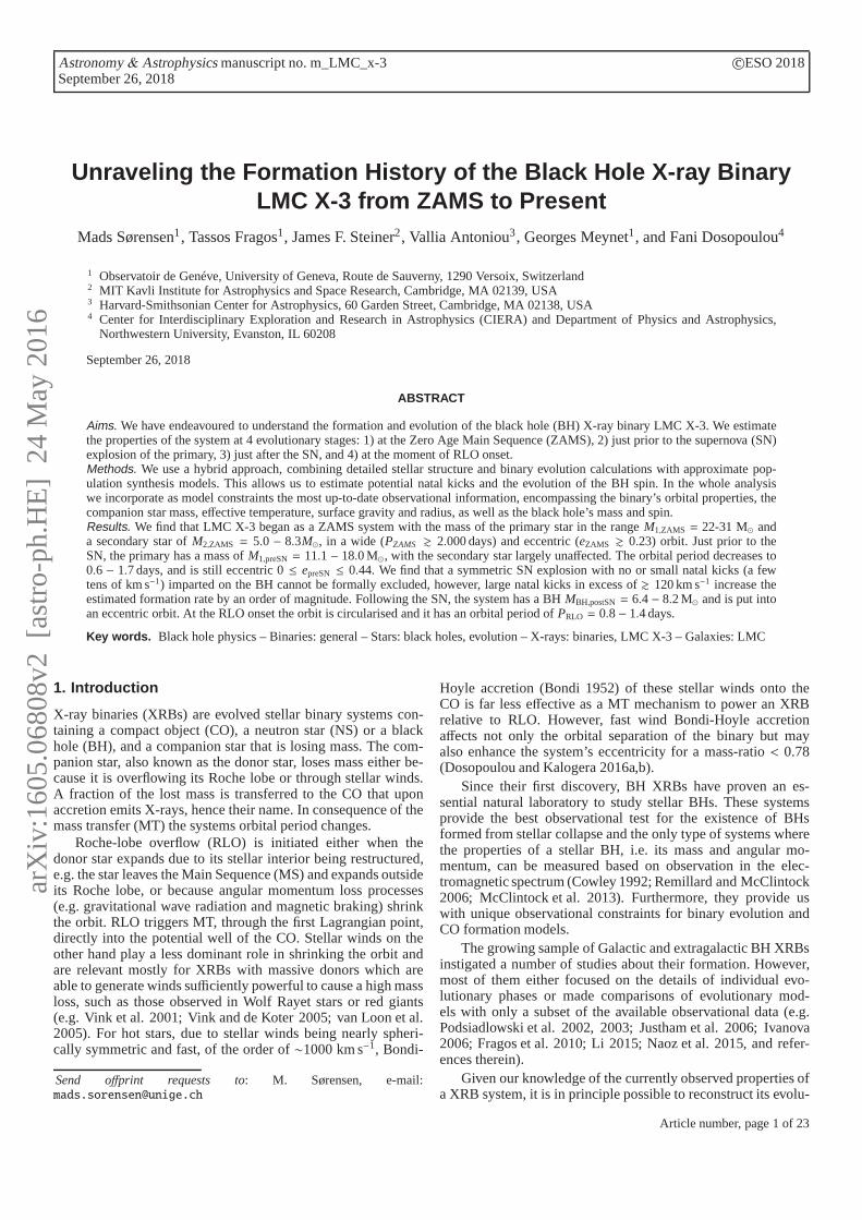
Fig. 1. The evolution of the BH spin parameter, given by eq. (9), for aset of BH initial massesMi , as a function of accreted massM0 eq. (10).The grey areas mark the 1σ and 2σ errors centered on the observed spinparameter for LMC X-3 (see Table 1). The vertical dashed black linesindicate the maximum allowed accreted massM0, at 2σ limit, for an ini-tial non-spinning BH mass of 5 M⊙ (left) and 8 M⊙ (right) respectively.

The solution of eq. (9) is shown in Fig. 1, for different initialBH masses at RLO onset. Here the evolution of the BH spin pa-rameter is tracked as a function of accreted mass. For reference,centered on the LMC X-3 spin parametera∗ = 0.25, we haveadded the 1σ and 2σ error region as the dark and light gray ar-eas respectively. One notes how a small initial BH mass requiresless accreted mass, in absolute terms, to build up its spin parame-ter compared to higher initial BH masses. As an example we canfollow a BH with initial massMi = 5.0M⊙ (blue line) as it ac-cretes mass and compare it to a BH with initial massMi = 8.0M⊙(black line). The blue line reaches the upper spin parameterhav-ing accreted∼ 1M⊙ reaching a current mass of 6M⊙. The blackline reaches the upper spin parameter limit when it has accreted∼ 1.6M⊙ and has a mass of 9.6M⊙. In terms of relative mass ac-creted to initial BH mass both BHs accrete∼ 20% of their initialBH mass before reaching the upper spin parameter limit of LMCX-3, so their initial BH mass was∼ 83.3% of the current masswhen accretion began. Hence, the maximum amount of accretedmaterial onto the BH of LMC X-3 is∼ 16.6% of its currentmass. The LMC X-3 BH has a lower mass limitMBH = 5.86M⊙within 2σ. A lower limit of the BH mass at RLO onset thereforebecomes (1− 0.166)5.86M⊙ ∼ 4.9M⊙.

If we instead consider the observed mass of the LMC X-3BH and accept a 2σ limit, its current upper mass limit is 8.1M⊙.Thus, a BH of initial mass 8.0M⊙ cannot have accreted morethan 0.1M⊙ suggesting such a BH in the case of LMC X-3 shouldhave a spin parametera∗ ∼ 0.04.

We stress here, we are using the observed BH spin of LMCX-3 only as a condition to constrain theupper limit of the amountof mass that the BH can possibly have accreted since the onsetofthe RLO. In reality, the BH in LMC X-3 may have been formedwith a non-zero natal spin, in which case the limits on the maxi-mum accreted mass discussed above would be upper bounds.

In summary, we note that the analytic point-mass MT modeltogether with the BH spin parameter is a powerful yet computa-tional inexpensive tool to establish rough but meaningful boundson our 5-dimensional parameter space in determining whether aset of initial conditions at RLO onset lead to a MT sequence thatsatisfies the observational constraints onPobs, MBH, andM2. Toaccount for the remaining observational constraints, X-ray lu-

Article number, page 5 of 23

A&A proofs:manuscript no. m_LMC_x-3

minosity,Teff , R2, logg2, and donor luminosityL2, we need tomodel in detail the stellar evolution of the companion star.

3.2. Detailed MESA calculation

Our detailed simulations of the MT phase between the donorstar and the BH are done with MESA, a state-of-the-art, pub-licly available, 1-D stellar structure and binary evolution code.We adopted a metallicity for the donor star appropriate for LMCstars (Z=0.006; which is in line with derived metallicities of stel-lar populations in LMC Antoniou and Zezas 2016) and used theimplicit MT scheme incorporated in MESA. All our simulationswere done with revision 7184 of the code1. We explored the ini-tial parameter space at the onset of RLO by constructing a gridof MT sequences forM2,RLO in the range 2-15M⊙ in steps of0.2 M⊙, orbital periodsPRLO from 0.6-4.2 days in steps 0.1 day,andMBH,RLO from 5.0-8.0M⊙ in steps of 0.5M⊙. Furthermore,we vary the accretion efficiency parameterβ, considering val-ues ofβ=0.0, 0.25, 0.5, 0.75, 0.9, and 1.0. In all our calcula-tions we set the accretion efficiency parameterα = 0.0, as a non-zero value would be appropriate only for massive donor starsthat lose a significant amount of mass in the form of fast stellarwinds (van den Heuvel 1994). To speed up the computation ofindividual models we have invoked a stopping criterion withinMESA which terminates the computation once the orbital pe-riod is above 6 days. Out of all possible combinations ofM2,RLO,MBH,RLO, PRLO andβ, we only run detailed MESA calculationsfor those sets of initial conditions that “passed” our analytic MTmodel test, described in Sect. 3.1.

To identify those MT sequences that are PPS of LMC X-3 atthe moment of RLO onset we perform the following checks:

1. The ZAMS radius of the donor star is smaller than its Rochelobe radius at the onset of RLO.

2. When RLO begins the donor star’s age is less than the age ofthe Universe (<13.7 Gyr). Furthermore, the MT calculationsare terminated when the age of the donor reaches 13.7 Gyr,so the system today cannot be older than the age of the Uni-verse either. In practice, neither of these constraints limit ourcalculations here, due to the range of donor star masses thatwe are exploring.

3. During the MT phase, as the orbital period is evolving, itshould cross the observed periodPobs.

4. A MT sequence modelI has j = [1, 5] predicted parameterswhich all must be within 2σ of the observed quantitiesµjgiven their associated errorsσj both listed in Table 1

|Ii, j − µ j)|σ j

≤ 2 (12)

whereIi,j are the predictions of theith MT sequence for eachof these quantities, at the time when the orbital period of theMT sequence is equal to the observed one.

5. Infer whether the predicted accretion rate onto the BH by thespecific MT system would cause it to appear as a transient ora persistent X-ray source.

The latter check separates the MT sequences into tworegimes of MT mechanisms. If the accretion rate onto the BHis MBH < MBH,crit, where

MBH,crit ≈ 10−5

(

MBH

M⊙

)0.5 (

M2

M⊙

)−0.2 (

P1yr

)1.4 M⊙yr, (13)

1 The detailed MESA settings used in out simulations can be found athttp://mesastar.org/results

the system is in a transient state, otherwise the system is ina per-sistent state (Dubus et al. 1999). A persistent source has a con-tinuous flow of material from the donor star to the BH, which al-lows for a relatively high luminosity. If the source is transient, itgoes through periods of outbursts of high X-ray flux but spendsmost of its time with little to no X-ray flux, i.e. in a quiescentphase.

Under the assumption of constant MT efficiency, i.e. constantα andβ, MT sequences passing checks 1 through 4 are PPS thatpredict a system with the characteristics similar to currently ob-served properties of LMC X-3. In principleα andβ are averagevalues for the efficiency of the MT and therefore merely serve asan indicator of whether a semi-conservative or non-conservativetransfer of mass is needed.

Assuming that the reported errors for all observed quantitiesin Table 1 are Gaussian, then the likelihood of a model MT se-quence,Ii , given the currently observed data,D, of LMC X-3can be written as:

Li(Ii|D) =∏

j=1,5

G(Ii, j; µ j, σ j), (14)

whereG is a normalised Gaussian function, andµj andσj for j =[1, 5] are the observed values and the associated errors listed inTable 1. In principle, the likelihood of a MT sequence, when thesequence is crossing the observed period, is an estimate of howclose the specific model MT sequence comes to the observedproperties of LMC X-3. We intend to use eq. (14) as a weight toproduce a series of probability density functions (PDF) in Sect.4.2. In this case, we also multiply the likelihood value calculatedby eq. (14) by the time period,∆T , that a model MT sequencespent close to the observed orbital period. This time periodisdefined as the total time during which all parametersj are within2σ of the observed properties.

3.3. Constraining the Properties of LMC X-3 progenitor atthe Onset of Roche Lobe Overflow

With the checks defined in the previous section we now presentthree examples of individual MT sequences and compare theseto the observational parameters in Table 1. The examples arechosen to demonstrate how the constraints select some MT se-quences as PPS and discard others.

All three examples are plotted together in Fig. 2 and have ini-tial parameters at the onset of RLO:β=0.75,MBH,RLO = 6.5M⊙,M2,RLO = 7.8M⊙, andPRLO = 1.0days (dotted lines);β=0.90,MBH,RLO = 6.0M⊙, M2,RLO = 7.4M⊙, and PRLO = 0.8days(dashed lines);β=0.90, MBH,RLO = 6.0M⊙, M2,RLO = 8.0M⊙,andPRLO = 0.8days (solid lines). Along the x-axis of all pan-els is the orbital periodP in days and the vertical dashed linemarks the currently observed orbital periodPorb (see Table 1).The color bar shows the relative likelihoodLi/Lmax, as deter-mined from eq. (14) for all parametersj. For all three examples,a maximum likelihood is reached as the MT sequence modelcrosses the observed orbital period. In each panel, (a) through(h), a thickening of the color indicates that all parametersIi,japart from the one being plotted, as indicated on each y-axis,are within 2σ of the observed value. The grey areas shown insome of the panels indicate the 1σ and 2σ (dark and light grey,respectively) error regions of those parameters centered on theobserved values, similar to Fig. 1.

Panel(a) of Figure 2 shows the evolution of the donor star’seffective temperature with orbital period. The solid and dashedlines are within 2σ of Teff,obs as they cross the observed orbital

Article number, page 6 of 23

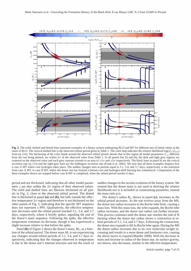
Mads Sørensen et al.: Unraveling the Formation History of the Black Hole X-ray Binary LMC X-3 from ZAMS to Present

1.0 1.5 2.0 2.5 3.0 3.5

12000

14000

16000

18000

20000

Teff (K)

a) a) a)

1.0 1.5 2.0 2.5 3.0 3.5

3.5

4.0

4.5

5.0

5.5

6.0

6.5

R2 (R

⊙)

c)c)c)

1.0 1.5 2.0 2.5 3.0 3.50.5

1.0

1.5

2.0

2.5

3.0

q−1

e)e)e)

0.5 1.0 1.5 2.0 2.5 3.0 3.5 4.0

period (days)

0.0

0.1

0.2

0.3

0.4

0.5

a∗

g)g)g)

1.0 1.5 2.0 2.5 3.0 3.5

2.5

3.0

3.5

4.0

4.5

5.0

5.5

M2 (M

⊙)

b) b) b)

1.0 1.5 2.0 2.5 3.0 3.5

−8.0

−7.5

−7.0

−6.5

−6.0

−5.5

logM

2 (M

⊙/yr)

d) d) d)

1.0 1.5 2.0 2.5 3.0 3.5

6.0

6.5

7.0

7.5

8.0

MBH (M

⊙)

f) f) f)

0.5 1.0 1.5 2.0 2.5 3.0 3.5 4.0

period (days)

−8.5

−8.0

−7.5

−7.0

−6.5

logM

BH (M

⊙/yr)

h) h) h)

β=0.75, MBH=6.5, M2=7.8, Porb=1.0 β=0.9, MBH=6.0, M2=7.4, Porb=0.8 β=0.9, MBH=6.0, M2=8.0, Porb=0.8

37.0

37.5

38.0

38.5

39.0

39.5

logL

(erg/s)

>-50 -40 -30 -20 -10 -5

log(Li(P)/Lmax)

Fig. 2. The solid, dashed and dotted lines represent examples of a binary system undergoing RLO and MT for different sets of initial values at theonset of RLO. The vertical dashed line is the observed orbital period given in Table 1. The color map indicates the relative likelihood log(Li/Lmax)from eq. (14). The thickening of the color bands around the observed orbital period, denote that in this region all model parametersIi, j, differentfrom the one being plotted, are within 2σ of the observed value from Table 1. In all panels but (f) and (h), the dark and light grey regions arecentered on the observed value and each grey contrast extends to an area of±1σ and±2σ respectively. The black lines in panel h) are the criticalaccretion rate eq. (13) and the light-grey lines are the Eddington accretion rate (Frank et al. 2002). We note that all three examples displays firsta case A MT where core hydrogen takes place. The sudden changes seen at periods equal to 3.1, 3.4, and 3.7 days, respectively, is the transitionfrom case A MT, to case B MT, where the donor star has formed a helium core and hydrogen-shell burning has commenced. Computation of thethree examples shown are stopped before case B MT is completed, when the orbital period reaches 6 days.

period and are thickened, indicating that all other model param-eters j are also within the 2σ region of their observed values.The solid and dashed lines are likewise thickened on all pan-els in Fig. 2, close to the observed orbital period. The dottedline is thickened in panel(a) and(b), but falls outside the effec-tive temperature 2σ region and therefore is not thickened on theother panels of Fig. 2, indicating that the specific MT sequencedoes not represent a PPS. Qualitatively, the effective tempera-ture decreases until the orbital period reached 3.1, 3.4, and 3.7days, respectively, where it briefly spikes, signaling the end ofthe donor’s main sequence. Following the spike, the effectivetemperature continues its decrease, though it has experienced aslight increase relative to that before the spike.

Panel(b) of Figure 2 shows the donor’s mass,M2, as a func-tion of the orbital period. The donor massM2 is not experiencingany changes around orbital periods of 3.1, 3.4, and 3.7 days re-spectively, indicating that the changes observed in temperatureis due to the donor star’s internal structure and not the result of

sudden changes in the secular evolution of the binary system. Weremind that the donor mass is not used in deriving the relativelikelihoods nor is it included as constraining parameter, insteadthe mass ratioq is.

The donor’s radiusR2, shown in panel(c), increases as theorbital period increases. As the star evolves away from the MS,the donor star radius increases to the Roche lobe limit, causing amass loss. With this mass loss, the orbit expands, the Roche loberadius increases, and the donor star radius can further increase.This process continues until the donor star reaches the end of Hburning where the donor star radius shows a contraction at or-bital periods of 3.1, 3.4, and 3.7 days. Following the contraction,the donor star expands to fill its Roche lobe again. During theMSthe donor radius increases due to its core molecular weight in-creasing and results in a more dense and luminous core, causingthe above layers to expand (Maeder 2008). With the decrease inmass and increase in radius of the donor star, its surface gravity,not shown, also decreases, similar to the effective temperature.

Article number, page 7 of 23

A&A proofs:manuscript no. m_LMC_x-3

In contrast to the mass of the donor star monotonically de-creasing, the evolution of mass loss rateM2, shown in panel(d)of Fig. 2 varies widely. It begins with a rapid turn-on phase,whenthe donor star fills its Roche lobe, and then gradually declines asthe mass-ratio of the binary decreases. The initial turn-onphaserapidly reaches a peak MT rate near 10−6 M⊙ yr−1 and then dropsby nearly an order of magnitude, where it stabilises to a steadyslow decrease until an orbital period of 3.1 days for the solidline, 3.4 days for the dashed, and 3.7 days for the dotted lines.At this point, the rate drops below 10−10 M⊙ yr−1 and the binarytemporarily detaches, but MT commences again with a rate of∼ 10−5.5 M⊙ yr−1, which is roughly sustained until the whole en-velope of the donor star is removed (see also Sect. 5.5 wherethe evolution of LMC X-3 after its currently observed state isdescribed). The mass loss rate of the donor starM2 qualitativelydictates the accretion rate onto the BH shown in panel(h) of Fig.2 but is larger by a factor (1− β)−1·

Panel(e) of Fig. 2 shows the change in the systems massratio which increases as material is transferred to the BH orislost from the system. For the three examples shown, both theirmass ratio and donor mass at the orbital period is within 2σ.However, there are combinations of donor mass and BH massfor which the mass ratio is outside the 2σ region.

In panel(f) of Fig. 2, we show the evolution of the BH’smass as a function of orbital period. The accretion onto the BHis initially mildly super-Eddington, but declines rapidly. Espe-cially for the dashed and solid lines withβ=0.9, it is seen that theBH mass-accretion rate reaches a plateau with only a small gainin mass as the orbital period lengthens. For the solid line withβ=0.75 the BH mass increase is larger, while at the same timethe orbit expands faster. All three lines satisfy the observed BHmass constraint at the crossing period. The BH spina∗, shownin panel(g), is a measure of the accreted angular momentum bythe BH, as we assumed a zero natal BH spin. We find that theevolution of the BH spin follows the characteristics of the BHmass, i.e. the growth in spin is steep initially and flattens as theorbital period increases.

Finally, panel(h) shows the BH mass accretion rate as afunction of orbital period. The light grey lines are the Eddingtonaccretion rates (Frank et al. 2002) and in black are the criticalaccretion rates (eq. (10)), that separate transient from persistentbehavior based on the thermal disk instability model, for eachMT sequence. The changes in the BH mass accretion rate withorbital period are similar to the mass loss rate of the compan-ion star, however, scaled with the value close toβ which is thefraction of transferred mass that is lost from the system in thevicinity of the BH. The solid line predicts a system which is inthe transient state, though not until an orbital period above∼1.65days. Both the dashed and dotted lines are predicted to be per-sistent systems when they cross the observed orbital period. TheBH accretion rate is also affected by the companion star’s sud-den change in radius and effective temperature, at orbital periodsof 3.1, 3.4, and 3.7 days, respectively. Following the second MTturn-on event, the BH in the three example sequences accreteclose to the Eddington accretion rate and are potentially mildlysuper-Eddington.

The three examples shown in Fig. 2 all show the same qual-itative evolution, but due to the differences in their initial con-ditions display the changes at different orbital periods. The ra-dial contraction seen in symphony with the increase in effec-tive temperature and surface acceleration, at 3.1, 3.4, and3.7days, indicates that the donor star is restructuring its interior. Itscore has depleted its hydrogen, stopped nuclear burning, and leftbehind a helium core. As a result, the core luminosity briefly

drops, whereby the envelope contracts, i.e. the donor radius de-creases, and the effective temperature and surface accelerationincrease. As a consequence of the contraction, a shell of hydro-gen at the bottom of the envelope ignites, pushing the envelopebeyond its pre-contraction radius. Hence the three examples inFig. 2 are case A RLO MT until an orbital period of 3.1, 3.4,and 3.7 days, where the hydrogen shell burning forces the enve-lope outwards and the three example enter a RLO MT of case B(Kippenhahn and Weigert 1967). In single star evolution, a starentering the hydrogen shell burning increases its radius dramat-ically, by approximately two orders of magnitude (Tauris 2006),and the star enters the Red Giant Branch (RGB). But due to thepresence of the BH, the RLO prevents the donor star to evolveinto the RGB phase. The donor star on one hand loses mass,increasing its Roche limit, and on the other hand inflates duetoits secular evolution which will shrink its Roche limit. Near shellburning ignition the donor star has lost∼60% of its ZAMS mass.Due to our stop criteria at an orbital period of 6 days, the threeexamples shown in Fig. 2 are not entering the helium burningphase. Though not shown, the rate of change in orbital periodduring case A MT is slow and during the case B MT phase in-creases dramatically, such that the entire evolution shownduringcase B MT in Fig. 2 only takes a few 105 yr. The donor star, inour three examples, has lost as much as∼70% of its ZAMS massby the time our simulations stop. For our MT sequences we ex-pect the donor star’s stellar evolution to end with the formationof a He White Dwarf (WD) or in the cases of the most massivedonors a Carbon Oxygen WD.

By reviewing the evolution of three selected MT sequencemodels, one that passes items 1-3 (dotted line), defined in Sect.3.2, two that pass items 1-4, we find confidence in our checksas a filter to locate PPS of LMC X-3 at the moment of RLOonset. As we also show, we can discriminate between transientand persistent systems. The calculated relative likelihood showsa maximum for all three examples close to the orbital period,avalidation of our approach. We next look at the overall result ofour detailed MT sequences.

3.4. Results of modelling the X-ray binary phase

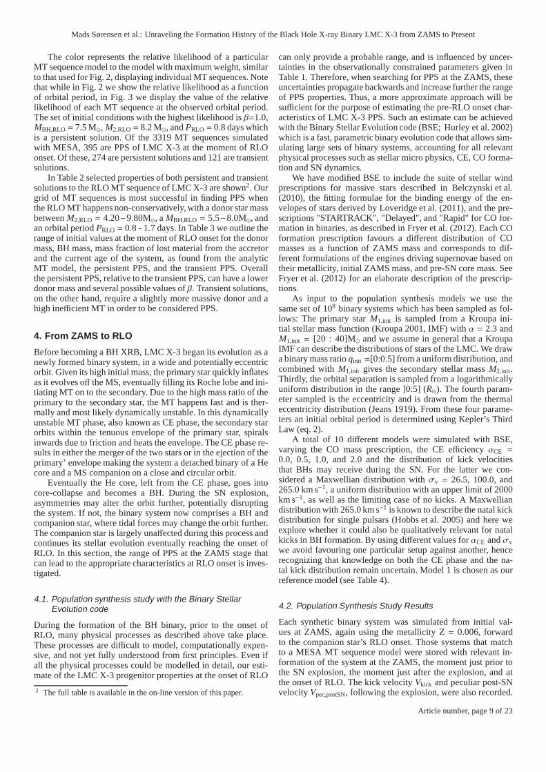
In Fig. 3, initial conditions of our grid of 3319 MT sequencesare shown. Each column of panels represents MT sequences fordifferent values ofβ (top axis). Each row varies the initial valueof MBH,RLO in units ofM⊙ (right axis). On the x-axis within eachpanel are plotted the companion massM2,RLO in units ofM⊙ andon the y-axis the orbital periodPRLO in days. The grey areas in-dicate regions where any combination of initial values fails theanalytic MT model. The white areas denote combinations of ini-tial values which pass the analytic MT model. As one increasesβ, the relative size of the area passing the analytic model in-creases. As a result we allow the horizontal size of each paneland x-axis range to change withβ in order to better display thecontent of each figure.

Each circle, square, and triangle represents a set of initialconditions of a binary system right before initiation of RLOthat was simulated with MESA. Circles are those MT sequenceswhich fail check 4. Those sequences that pass all checks and arepersistent solutions are shown as squares, while trianglesdenotethose sequences that pass all checks and are transient solutions.It is clearly shown in the figure that the number of PPS increaseswith β. Whereas persistent solutions (squares) can be found forall values ofβ exceptβ=1.0, transient solutions are only foundfor β=0.9 andβ=1.0, indicating that if LMC X-3 is a transientsource the ongoing MT is highly non-conservative.

Article number, page 8 of 23

Mads Sørensen et al.: Unraveling the Formation History of the Black Hole X-ray Binary LMC X-3 from ZAMS to Present

The color represents the relative likelihood of a particularMT sequence model to the model with maximum weight, similarto that used for Fig. 2, displaying individual MT sequences.Notethat while in Fig. 2 we show the relative likelihood as a functionof orbital period, in Fig. 3 we display the value of the relativelikelihood of each MT sequence at the observed orbital period.The set of initial conditions with the highest likelihood isβ=1.0,MBH,RLO = 7.5 M⊙, M2,RLO = 8.2 M⊙, andPRLO = 0.8 days whichis a persistent solution. Of the 3319 MT sequences simulatedwith MESA, 395 are PPS of LMC X-3 at the moment of RLOonset. Of these, 274 are persistent solutions and 121 are transientsolutions.

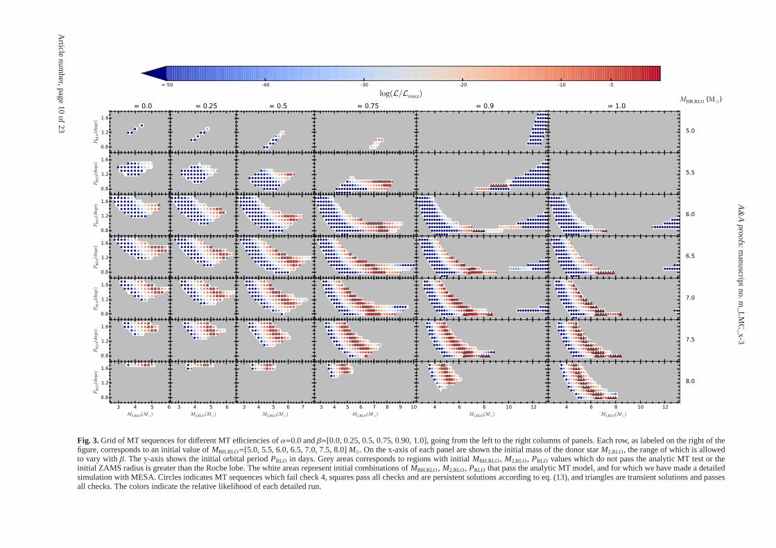
In Table 2 selected properties of both persistent and transientsolutions to the RLO MT sequence of LMC X-3 are shown2. Ourgrid of MT sequences is most successful in finding PPS whenthe RLO MT happens non-conservatively, with a donor star massbetweenM2,RLO = 4.20−9.80M⊙, aMBH,RLO = 5.5−8.0M⊙, andan orbital periodPRLO = 0.8 - 1.7 days. In Table 3 we outline therange of initial values at the moment of RLO onset for the donormass, BH mass, mass fraction of lost material from the accretorand the current age of the system, as found from the analyticMT model, the persistent PPS, and the transient PPS. Overallthe persistent PPS, relative to the transient PPS, can have alowerdonor mass and several possible values ofβ. Transient solutions,on the other hand, require a slightly more massive donor and ahigh inefficient MT in order to be considered PPS.

4. From ZAMS to RLO

Before becoming a BH XRB, LMC X-3 began its evolution as anewly formed binary system, in a wide and potentially eccentricorbit. Given its high initial mass, the primary star quicklyinflatesas it evolves off the MS, eventually filling its Roche lobe and ini-tiating MT on to the secondary. Due to the high mass ratio of theprimary to the secondary star, the MT happens fast and is ther-mally and most likely dynamically unstable. In this dynamicallyunstable MT phase, also known as CE phase, the secondary starorbits within the tenuous envelope of the primary star, spiralsinwards due to friction and heats the envelope. The CE phase re-sults in either the merger of the two stars or in the ejection of theprimary’ envelope making the system a detached binary of a Hecore and a MS companion on a close and circular orbit.

Eventually the He core, left from the CE phase, goes intocore-collapse and becomes a BH. During the SN explosion,asymmetries may alter the orbit further, potentially disruptingthe system. If not, the binary system now comprises a BH andcompanion star, where tidal forces may change the orbit further.The companion star is largely unaffected during this process andcontinues its stellar evolution eventually reaching the onset ofRLO. In this section, the range of PPS at the ZAMS stage thatcan lead to the appropriate characteristics at RLO onset is inves-tigated.

4.1. Population synthesis study with the Binary StellarEvolution code

During the formation of the BH binary, prior to the onset ofRLO, many physical processes as described above take place.These processes are difficult to model, computationally expen-sive, and not yet fully understood from first principles. Even ifall the physical processes could be modelled in detail, our esti-mate of the LMC X-3 progenitor properties at the onset of RLO

2 The full table is available in the on-line version of this paper.

can only provide a probable range, and is influenced by uncer-tainties in the observationally constrained parameters given inTable 1. Therefore, when searching for PPS at the ZAMS, theseuncertainties propagate backwards and increase further the rangeof PPS properties. Thus, a more approximate approach will besufficient for the purpose of estimating the pre-RLO onset char-acteristics of LMC X-3 PPS. Such an estimate can be achievedwith the Binary Stellar Evolution code (BSE; Hurley et al. 2002)which is a fast, parametric binary evolution code that allows sim-ulating large sets of binary systems, accounting for all relevantphysical processes such as stellar micro physics, CE, CO forma-tion and SN dynamics.

We have modified BSE to include the suite of stellar windprescriptions for massive stars described in Belczynski etal.(2010), the fitting formulae for the binding energy of the en-velopes of stars derived by Loveridge et al. (2011), and the pre-scriptions "STARTRACK", "Delayed", and "Rapid" for CO for-mation in binaries, as described in Fryer et al. (2012). EachCOformation prescription favours a different distribution of COmasses as a function of ZAMS mass and corresponds to dif-ferent formulations of the engines driving supernovae based ontheir metallicity, initial ZAMS mass, and pre-SN core mass.SeeFryer et al. (2012) for an elaborate description of the prescrip-tions.

As input to the population synthesis models we use thesame set of 108 binary systems which has been sampled as fol-lows: The primary starM1,init is sampled from a Kroupa ini-tial stellar mass function (Kroupa 2001, IMF) withα = 2.3 andM1,init = [20 : 40]M⊙ and we assume in general that a KroupaIMF can describe the distributions of stars of the LMC. We drawa binary mass ratioqinit =[0:0.5] from a uniform distribution, andcombined withM1,init gives the secondary stellar massM2,init .Thirdly, the orbital separation is sampled from a logarithmicallyuniform distribution in the range ]0:5] (R⊙). The fourth param-eter sampled is the eccentricity and is drawn from the thermaleccentricity distribution (Jeans 1919). From these four parame-ters an initial orbital period is determined using Kepler’sThirdLaw (eq. 2).

A total of 10 different models were simulated with BSE,varying the CO mass prescription, the CE efficiency αCE =

0.0, 0.5, 1.0, and 2.0 and the distribution of kick velocitiesthat BHs may receive during the SN. For the latter we con-sidered a Maxwellian distribution withσv = 26.5, 100.0, and265.0 km s−1, a uniform distribution with an upper limit of 2000km s−1, as well as the limiting case of no kicks. A Maxwelliandistribution with 265.0 km s−1 is known to describe the natal kickdistribution for single pulsars (Hobbs et al. 2005) and hereweexplore whether it could also be qualitatively relevant fornatalkicks in BH formation. By using different values forαCE andσvwe avoid favouring one particular setup against another, hencerecognizing that knowledge on both the CE phase and the na-tal kick distribution remain uncertain. Model 1 is chosen asourreference model (see Table 4).

4.2. Population Synthesis Study Results

Each synthetic binary system was simulated from initial val-ues at ZAMS, again using the metallicity Z= 0.006, forwardto the companion star’s RLO onset. Those systems that matchto a MESA MT sequence model were stored with relevant in-formation of the system at the ZAMS, the moment just prior tothe SN explosion, the moment just after the explosion, and atthe onset of RLO. The kick velocityVkick and peculiar post-SNvelocityVpec,postSN, following the explosion, were also recorded.

Article number, page 9 of 23

A&

Aproofs:m

anuscriptno.m_L

MC

_x-3

0.8

1.2

1.6

PRLO(days)

β = 0.0 β = 0.25 β = 0.5 β = 0.75 β = 0.9MBH,RLO (M⊙)

5.0

β = 1.0

0.8

1.2

1.6

PRLO(days)

5.5

0.8

1.2

1.6

PRLO(days)

6.0

0.8

1.2

1.6

PRLO(days)

6.5

0.8

1.2

1.6

PRLO(days)

7.0

0.8

1.2

1.6

PRLO(days)

7.5

3 4 5 6

M2,RLO(M⊙)

0.8

1.2

1.6

PRLO(days)

3 4 5 6

M2,RLO(M⊙)3 4 5 6 7

M2,RLO(M⊙)3 4 5 6 7 8 9 10

M2,RLO(M⊙)4 6 8 10 12

M2,RLO(M⊙)4 6 8 10 12

M2,RLO(M⊙)

8.0

<-50 -40 -30 -20 -10 -5

log(L/Lmax)

Fig. 3. Grid of MT sequences for different MT efficiencies ofα=0.0 andβ=[0.0, 0.25, 0.5, 0.75, 0.90, 1.0], going from the left to the right columns of panels. Each row, as labeled on the right of thefigure, corresponds to an initial value ofMBH,RLO=[5.0, 5.5, 6.0, 6.5, 7.0, 7.5, 8.0]M⊙. On the x-axis of each panel are shown the initial mass of the donor starM2,RLO, the range of which is allowedto vary withβ. The y-axis shows the initial orbital periodPRLO in days. Grey areas corresponds to regions with initialMBH,RLO, M2,RLO, PRLO values which do not pass the analytic MT test or theinitial ZAMS radius is greater than the Roche lobe. The whiteareas represent initial combinations ofMBH,RLO, M2,RLO, PRLO that pass the analytic MT model, and for which we have made a detailedsimulation with MESA. Circles indicates MT sequences whichfail check 4, squares pass all checks and are persistent solutions according to eq. (13), and triangles are transient solutions and passesall checks. The colors indicate the relative likelihood of each detailed run.

Article

number,page

10of23

Mads

Sø

rensenetal.:

Unraveling

theF

ormation

History

ofthe

Black

Hole

X-ray

Binary

LM

CX

-3from

ZA

MS

toP

resent

Table 2. Selected properties of some MT sequences that pass all criteria at the observed orbital period. The 10 MT sequences numbered between 175 to 206 are persistent solutions and the 10 MTsequences numbered between 1970 to 2224 are transient solutions. For all MT sequence modelsα = 0. A full list of all MT sequences found is available in the on line version.

Parameters at RLO onset Parameters at observed orbital period PorbMT

Sequence βa MBH,RLO

b M2,RLOc PRLO

d Xc,RLOe τRLO

f MBHb a∗g M2

c logL2h Xc

i τ log(L/Lmax)j ∆T k

(M⊙) (M⊙) (days) (Myr) (M⊙) (M⊙) (L⊙) (Myr) (Myr)175 0.0 8.0 4.6 1.7 0.12 86.26 8.02 0.01 4.57 3.00 0.09 87.91 -6.98 0.52188 0.0 7.0 4.8 1.6 0.14 77.56 7.29 0.13 4.50 2.99 0.12 78.62 -6.75 0.13190 0.0 7.5 4.8 1.6 0.18 74.75 7.80 0.13 4.49 2.99 0.12 78.52 -6.71 0.38191 0.0 7.5 4.8 1.7 0.14 77.56 7.55 0.02 4.74 3.06 0.10 79.77 -7.72 0.34192 0.0 8.0 4.8 1.7 0.14 77.56 8.04 0.02 4.75 3.06 0.10 79.65 -8.55 0.35200 0.0 6.5 5.0 1.5 0.18 68.30 7.14 0.28 4.35 2.96 0.15 70.16 -7.62 0.10203 0.0 7.0 5.0 1.5 0.18 68.30 7.60 0.25 4.39 2.97 0.15 70.38 -6.80 0.40204 0.0 7.0 5.0 1.6 0.18 68.30 7.36 0.16 4.63 3.03 0.13 71.47 -7.24 0.20205 0.0 7.5 5.0 1.5 0.18 68.30 8.04 0.22 4.45 2.99 0.15 70.52 -7.04 0.41206 0.0 7.5 5.0 1.6 0.18 68.30 7.82 0.14 4.67 3.05 0.13 71.47 -7.64 0.27

1970 0.9 8.0 4.6 1.7 0.12 86.26 8.00 0.00 4.58 3.01 0.09 87.91 -6.94 6.012010 0.9 8.0 4.8 1.7 0.14 77.56 8.00 0.00 4.77 3.07 0.10 79.66 -8.82 0.362178 0.9 7.0 6.4 0.8 0.58 15.60 7.24 0.11 3.98 2.92 0.22 48.42 -5.33 1.312181 0.9 7.5 6.4 0.8 0.58 15.60 7.73 0.10 4.08 2.95 0.22 47.86 -4.79 1.752182 0.9 7.5 6.4 0.9 0.50 22.50 7.73 0.10 4.05 2.95 0.22 45.98 -4.69 1.792189 0.9 7.0 6.6 0.8 0.58 14.46 7.25 0.12 4.05 2.95 0.22 45.89 -4.27 1.912198 0.9 6.5 6.8 0.8 0.58 13.47 6.78 0.14 3.97 2.94 0.23 44.59 -5.05 1.872199 0.9 6.5 6.8 0.9 0.51 19.44 6.79 0.14 3.91 2.93 0.24 42.64 -5.01 1.862215 0.9 6.0 7.2 0.8 0.58 11.83 6.33 0.17 3.86 2.92 0.23 42.83 -6.66 2.002224 0.9 6.0 7.4 0.8 0.60 9.56 6.35 0.18 3.89 2.94 0.23 41.57 -6.04 2.46

Notes. The parameters at the crossing periodPorb correspond to those the binary system is believed to have currently.(a) Fraction of transferred mass lost from BH.(b) BH mass.(c) Donor mass.(d) Orbital period.(e) Fraction of hydrogen in core of the donor.(f) Age of donor.(g) BH spin.(h) Luminosity of donor.(j) Fraction of element H left in core.(j) Total weight for MT sequence from eq. (14)(k) Time spent around the observed orbital period.

Article

number,page

11of23

A&A proofs:manuscript no. m_LMC_x-3

Table 3. List of PPS property ranges at the RLO onset found from MT sequences with the analytic model and MESA respectively. Results fromMESA has been divided into persistent and transient systems(see text).

Parameter Analytic model MESAPersistent Transient

PRLO (days) 0.70 - 2.80 0.80 - 1.70 0.80 - 1.70M2,RLO (M⊙) 4.60 - 15.0 4.60 - 8.20 4.60 - 9.80

MBH,RLO (M⊙) 5.00 - 8.00 5.50 - 8.00 5.50 - 8.00β 0.00 - 1.00 0.00 - 0.90 0.90-1.00

τ (Myr) - 33.53 - 88.52 36.09 - 87.90

Table 4. Setup of our population synthesis models using BSE (first 5 columns). The number of PPS found are shown in Col. 6. Column 7 showsthe expected number of IMXB in the LMC today, see Sect. 4.4. COprescription refers to those given in Fryer et al. (2012),αCE is the CE efficiencyparameter. We have used two SN kick velocity distributions.For the Maxwellian distributionσv is the most probable kick velocity and for theuniform distribution it refers to the upper kick limit.σv = 0 means no natal kicks imparted onto the BH.

Model CO prescription αCE Velocity distribution σv (km s−1) NPPS NIMXB

1 Rapid 1.0 Maxwellian 265.0 1322 0.722 Rapid 0.1 Maxwellian 265.0 1 0.213 Rapid 0.5 Maxwellian 265.0 557 0.424 Rapid 2.0 Maxwellian 265.0 5508 1.805 Rapid 1.0 Maxwellian 0.0 111 0.436 Rapid 1.0 Maxwellian 26.5 161 0.527 Rapid 1.0 Maxwellian 100.0 980 0.548 STARTRACK 1.0 Maxwellian 265.0 29 0.989 Delayed 1.0 Maxwellian 265.0 1222 0.7310 Rapid 1.0 uniform 2000.0 245 0.12

We define a match between MESA MT sequence and a singleBSE system if the system at the onset of RLO predicted by BSEare within 0.05 days of the orbital period, 0.1 M⊙ of the donormass, and 0.25 M⊙ of the BH mass, of one of the MT sequencessimulated with MESA. We only match BSE solutions with the395 MT sequences identified as LMC X-3 PPS from modellingthe X-ray MT phase, see Sect. 3.4. Of the 395 matching MT se-quences, 121 are solutions to LMC X-3 as a transient source andthe remaining 274 identified MT sequences are persistent solu-tions to LMC X-3.

The second rightmost column of Table 4 shows the num-ber of PPS for each population synthesis model. The referenceModel 1 generated 1322 PPS out of a total of 108 simulated bina-ries, suggesting at a first glance a relatively low formationrate,but see discussion in Sect. 4.1. In model 2, 3, and 4 we vary theCE efficiency parameter, withαCE = 0.1, 0.5, 2.0 for each modelrespectively, and we find that the number of PPS increases withαCE. In models 5, 6, and 7 we vary the distribution of natal BHkicks, with the most probable kick velocity beingσv = 0.0, 26.5and 100 km s−1 for each model respectively, also finding an in-creasing number of PPS with increasingσv. Model 8 adopts the"STARTRACK" prescription for the mass of CO formed, gen-erating a small number of PPS, while in model 9 the "Rapid"prescription for CO formation was used, producing a number ofPPS comparable to model 1.

The small number of PPS produced from models 2 and 8are statistically insignificant samples of PPS to robustly estimatethe range of LMC X-3 PPS at ZAMS. Based on the very lowformation efficiency of these two models, we can only infer thatit is plausible, but highly unlikely, that LMC X-3 is formed fromthe settings of these models. For LMC X-3 this suggests that theCE phase is necessary, and that the STARTRACK prescriptionis not a good estimate of CO masses. For model 4, which is the

model that most efficiently forms PPS, it is hard to justify thehigh value ofαCE, but it also points towards the CE phase beingimportant for generating LMC X-3 like systems. Since model2 produced only 1 PPS we do not include it in the rest of ouranalysis.

Based on the number of PPS for each model, we performa statistical analysis using weighted Kernel Density Estimators(KDE). A Gaussian kernel is used to produce a probability den-sity estimate for each relevant property of PPS during the evolu-tion of the LMC X-3. In Fig. 4 we demonstrate how the PDF ofthe companion stars’ mass at ZAMS,M2,ZMAS, will look for eachpopulation synthesis model for different weights. The weightsare found using a single factor in eq. (14), i.e. onlyIi,j and aweight based on the time a MT sequence spends around the cur-rently observed properties of LMC X-3. The latter is defined asthe time a MT sequence spends within two standard deviationsof all the observed constraints. Finally the total weight which isthe product, i.e. left hand side, of eq. (14)Ii multiplied by thetime spent around the observed orbital period. The gray bar plotis a normalised histogram and the dashed line is a non-weightedKDE. The remaining lines are KDEs with different weights asdescribed by the legend. It is shown that the unweighted KDEproduces a continuous distribution that follows closely the dis-crete distribution of the histogram. The total weight eq. (14) overall j, relative to the other distributions, concentrates the mostlikely solution into two peaks except for model 5, 6, and 8. Themost likely values based on the total weight also shows the twopeaks to fall away from the peak of the unweighted distribution,the cause of which is the emergent distribution of using countstogether with weights. The distribution using the total weightfinds a different maximum because the weights near the max-imum with no weights are much smaller, by several orders ofmagnitude, than the weights at the maximum of the distribution

Article number, page 12 of 23

Mads Sørensen et al.: Unraveling the Formation History of the Black Hole X-ray Binary LMC X-3 from ZAMS to Present

4 5 6 7 8 9 100.0

0.2

0.4

0.6

0.8

1.0

PDF

a) Model 1, NPPS = 1322

4 5 6 7 8 9 100.0

0.2

0.4

0.6

0.8

1.0

PDF

b) Model 3, NPPS = 557

4 5 6 7 8 9 100.0

0.5

1.0

1.5

2.0

PDF

d) Model 5, NPPS = 111

4 5 6 7 8 9 100.0

0.2

0.4

0.6

0.8

1.0

PDF

f) Model 7, NPPS = 980

4 5 6 7 8 9 10M2,ZAMS (M⊙)

0.0

0.2

0.4

0.6

0.8

1.0

PDF

h) Model 9, NPPS = 1222

4 5 6 7 8 9 10

c) Model 4, NPPS = 5508

no weight

qMBH

Teff

log10R

log10g

Time

Total

Histogram

4 5 6 7 8 9 10

e) Model 6, NPPS = 161

4 5 6 7 8 9 10

g) Model 8, NPPS = 29

4 5 6 7 8 9 10M2,ZAMS (M⊙)

i) Model 10, NPPS = 245

Fig. 4. The probability density function (PDF) of initial masses ofthe companion starM2,ZAMS for the different synthesis population models inTable 4. The grey bar is a normalised histogram and the different colored lines are normalised Kernel Density Estimates for different weights foundfrom eq. (14) and shown in the insert of this figure, for individual factorsj and for the total weight given as the product over allj times the timespent around the orbital period, which is the black line.

Article number, page 13 of 23

A&A proofs:manuscript no. m_LMC_x-3

with the total weight (see the color scale of Fig. 3 which displaysthe values of the total weights). In the remaining analysis we usethe total weight in all our distributions.

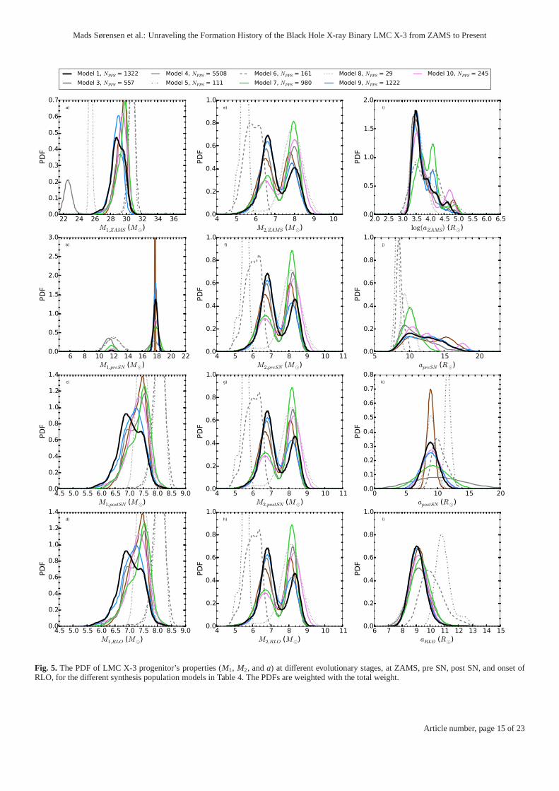
Figure 5 shows the overall most likely evolution of LMC X-3, from its initial binary properties at ZAMS (top panel), topre-SN (second row), post-SN (third row) and finally at RLO onset(bottom row), for the different population synthesis models, ex-pressed as PDFs. The PDFs are produced as KDEs with the totalweight applied, as defined earlier. Each color is a model fromTa-ble 4 (see the figure legend). We have de-emphasized four mod-els by presenting them in gray color. Three of these (models 5,6, and 8) because they have small or insufficient numbers of PPSto be statistical representable. Model 4 is also grayed out,but in-stead owing to its unphysical setting ofαce = 2. The latter modelwas considered mostly in order to examine the sensitivity ofthenumber of PPS to this parameter.

The remaining models 1, 3, 7, 9, and 10 have model parame-ters that are physically plausible and produce a sufficiently largenumber of PPS. These models estimate the values, at differentevolutionary stages, of LMC X-3 progenitor’s properties tobe inthe same range, along the x-axis of each panel. The peak of eachdistribution also seems to be at the same x-values, though, forplaces with a bimodal distribution, the individual model favorsthe peaks differently.

The initial value ofM1,ZAMS at the 95% percentile is in therange 25.4–31.0 M⊙ when considering all models except model4. Model 4 has a range 22.4–30.1 M⊙. All models suggest thatthe primary mass just prior to the SN is close toM1,preSN∼17.8M⊙, although models 4, 7, and 10 also suggest a minor peakaround∼12 M⊙. After the SN, the range of the CO masses isM1,postSN=6.4–8.2 M⊙ (95% percentile).

The secondary starM2 experiences less dramatic changes,compared to the primaryM1, evolving from a ZAMS to a BH.This is expected asM2 during this time is still on the MS andduring the first MT episode the secondary mass star does notgain significant mass. There are two most probable values forthedonor mass, one around 6.8 M⊙ favoured by model 1,3,4, and 9.The second peak is around 8 M⊙ and is favoured by models 7 and10. The mass range spanned by all models is 5.0–8.4M⊙ (95%percentile).

The orbital separation is initially very large, but as the pri-mary star evolves away from the MS it fills its Roche lobe, andthe binary gets into a CE phase, resulting in a significantly closerbinary orbit. At the moment just prior to the SN,a has decreasedby a factor of∼300, from several thousand solar radii to justaround∼10R⊙. The orbital separation following the SN, favoursa value around∼9R⊙.

The distribution of most likely kicks imparted during the BHformation is shown in Fig. 6 and the post SN peculiar veloc-ity shown in Fig. 7 which is due to both the kick imparted andthe mass loss. Models 1, 3, 4, and 9 suggest the same distribu-tion for the imparted kick and follow from the fact that these4 models had the same input distribution. The range of these4 models, is roughly betweenVkick=193–683km s−1 (95% per-centile), with only models 5, 6, and 7 suggesting kicks less than120 km s−1, which is expected given the smaller most probablekick value for these models. Thus, the actual lower limit ofVkickmay likely be closer to 120 km s−1. Notably, model 7, whichusesσv = 100 km/s still shows a peak kick at∼ 180 km/s,which is supportive of the demand for an appreciable kick in theBH formation. Model 10 applied an uniform kick distributionand finds PPS within the rangeVkick = 212-912 km s−1 (95%percentile). All in all the distribution ofVkick in the differentpopulation synthesis models indicates that a relative highkick

0 200 400 600 800 1000 1200 1400

Vkick (km/s)

0.000

0.005

0.010

0.015

0.020

0.025

PDF

Model 1

Model 3

Model 4

Model 6

Model 7

Model 8

Model 9

Model 10

0 100 200 300 400 500 600 700 8000.000

0.005

0.010

Fig. 6. The PDF of the kick imparted to LMC X-3 during the SN for thedifferent synthesis population studies. The insert gives a moredetailedview of the distribution in the x-axis range from 0 to 800 km/s andfollows the same axis labels and plotted the lines the same legend.

velocity is likely to be imparted to the LMC X-3 progenitor sys-tem. We do find in our simulations that some models producePPS with smaller or no kicks, but the associated probabilityislow relative to models favouring high kicks. The consequenceof the kick, assuming it does not disrupt the system, is a per-turbation of the system’s center of mass motion or the post SNpeculiar velocity. In addition to the kick, material lost from thesystem via the primary also affects the post SN peculiar veloc-ity Vpec,postSN (Kalogera 1996; Willems et al. 2005, see Fig. 7),as this mass is ejected off center of the binary system center ofmass. Overall theVpec,postSN in Fig. 7 is comparable in magni-tude to the kick velocity shown in Fig. 6. For all models, exceptmodel 7, more than 90% of the PPS haveVkick > Vpec,postSN. Inmodel 6 and 7 only∼ 11% and∼ 27% have a larger kick ve-locity thanVpec,postSN, and for models 5 theVpec,postSN is alwayslarger than the relatingVkick. For model 10 with a uniform kickdistribution∼ 99% haveVkick > Vpec,postSN.

4.3. Example of full evolution from ZAMS to White Dwarfformation

In Fig. 8 we illustrate the complete evolution of a typical LMCX-3 PPS, from ZAMS and until the companion star becomes aWD. The system chosen is the MESA MT sequence with rel-ative high likelihood for the X-ray binary phase and one of itsBSE matches for the evolution prior to the X-ray phase, hencerepresentative of our results. The evolution begins with a pri-mary star of massM1,ZAMS = 26.5 M⊙ and its companion starwith massM2=8 M⊙ in a wide and highly eccentric orbit. Theprimary star evolves quickly and fills its Roche lobe, leading toa CE phase which shrinks and circularises the orbit. During theCE phase the donor star spirals inwards within the primary enve-lope. Due to friction the envelope is heated and expelled leavingbehind a detached binary of a naked He core and the donor star.The remaining He core of the primary eventually experiencesa SN explosion at∼ 8 Myr and collapses into a BH. During theSN the BH receives a natal kickVkick = 497 km s−1. 4.2 Myr laterat time= 12.2 Myr, the companion star fills its Roche lobe andmass starts flowing from the donor star onto the BH. The sys-tem is now an observable X-ray source until a time of 58.8 Myr

Article number, page 14 of 23

Mads Sørensen et al.: Unraveling the Formation History of the Black Hole X-ray Binary LMC X-3 from ZAMS to Present

22 24 26 28 30 32 34 36M1,ZAMS (M⊙)

0.0

0.1

0.2

0.3

0.4

0.5

0.6

0.7

PDF

a)

6 8 10 12 14 16 18 20 22M1,preSN (M⊙)

0.0

0.5

1.0

1.5

2.0

2.5

3.0

PDF

b)

4.5 5.0 5.5 6.0 6.5 7.0 7.5 8.0 8.5 9.0M1,postSN (M⊙)

0.0

0.2

0.4

0.6

0.8

1.0

1.2

1.4

PDF

c)

4.5 5.0 5.5 6.0 6.5 7.0 7.5 8.0 8.5 9.0M1,RLO (M⊙)

0.0

0.2

0.4

0.6

0.8

1.0

1.2

1.4

PDF

d)

4 5 6 7 8 9 10M2,ZAMS (M⊙)

0.0

0.2

0.4

0.6

0.8

1.0

PDF

e)

Model 1, NPPS = 1322

Model 3, NPPS = 557

Model 4, NPPS = 5508

Model 5, NPPS = 111

Model 6, NPPS = 161

Model 7, NPPS = 980

Model 8, NPPS = 29

Model 9, NPPS = 1222

Model 10, NPPS = 245

4 5 6 7 8 9 10 11M2,preSN (M⊙)

0.0

0.2

0.4

0.6

0.8

1.0

PDF

f)

4 5 6 7 8 9 10 11M2,postSN (M⊙)

0.0

0.2

0.4

0.6

0.8

1.0

PDF

g)

4 5 6 7 8 9 10 11M2,RLO (M⊙)

0.0

0.2

0.4

0.6

0.8

1.0

PDF

h)

2.0 2.5 3.0 3.5 4.0 4.5 5.0 5.5 6.0 6.5log(aZAMS) (R⊙)

0.0

0.5

1.0

1.5

2.0

PDF

i)

5 10 15 20apreSN (R⊙)

0.0

0.2

0.4

0.6

0.8

1.0

PDF

j)

0 5 10 15 20apostSN (R⊙)

0.0

0.1

0.2

0.3

0.4

0.5

0.6

0.7

0.8

PDF

k)

6 7 8 9 10 11 12 13 14 15aRLO (R⊙)

0.0

0.2

0.4

0.6

0.8

1.0

PDF

l)

Fig. 5. The PDF of LMC X-3 progenitor’s properties (M1, M2, anda) at different evolutionary stages, at ZAMS, pre SN, post SN, and onset ofRLO, for the different synthesis population models in Table 4. The PDFs are weighted with the total weight.

Article number, page 15 of 23

A&

Aproofs:m

anuscriptno.m_L

MC

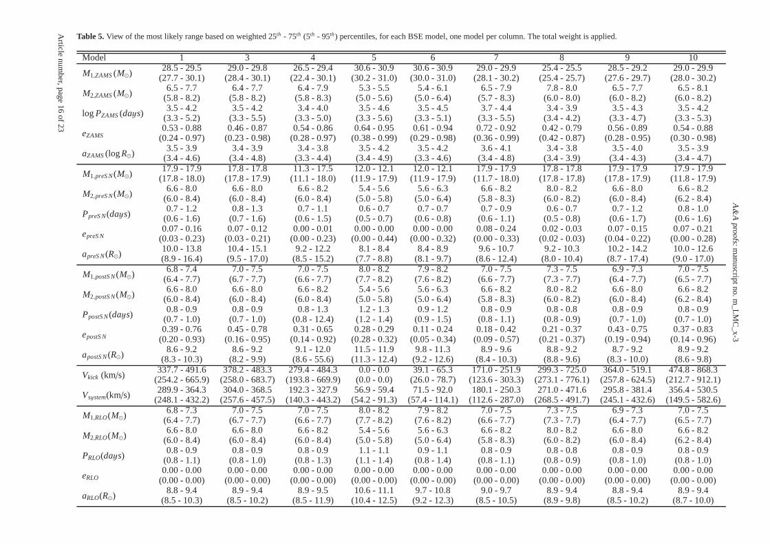
_x-3Table 5. View of the most likely range based on weighted 25th - 75th (5th - 95th) percentiles, for each BSE model, one model per column. The total weight is applied.

Model 1 3 4 5 6 7 8 9 10

M1,ZAMS (M⊙)28.5 - 29.5

(27.7 - 30.1)29.0 - 29.8

(28.4 - 30.1)26.5 - 29.4

(22.4 - 30.1)30.6 - 30.9

(30.2 - 31.0)30.6 - 30.9

(30.0 - 31.0)29.0 - 29.9

(28.1 - 30.2)25.4 - 25.5

(25.4 - 25.7)28.5 - 29.2

(27.6 - 29.7)29.0 - 29.9

(28.0 - 30.2)

M2,ZAMS (M⊙)6.5 - 7.7

(5.8 - 8.2)6.4 - 7.7

(5.8 - 8.2)6.4 - 7.9

(5.8 - 8.3)5.3 - 5.5

(5.0 - 5.6)5.4 - 6.1

(5.0 - 6.4)6.5 - 7.9

(5.7 - 8.3)7.8 - 8.0

(6.0 - 8.0)6.5 - 7.7

(6.0 - 8.2)6.5 - 8.1

(6.0 - 8.2)

logPZAMS (days)3.5 - 4.2

(3.3 - 5.2)3.5 - 4.2

(3.3 - 5.5)3.4 - 4.0

(3.3 - 5.0)3.5 - 4.6

(3.3 - 5.6)3.5 - 4.5

(3.3 - 5.1)3.7 - 4.4

(3.3 - 5.5)3.4 - 3.9

(3.4 - 4.2)3.5 - 4.3

(3.3 - 4.7)3.5 - 4.2

(3.3 - 5.3)

eZAMS0.53 - 0.88

(0.24 - 0.97)0.46 - 0.87

(0.23 - 0.98)0.54 - 0.86

(0.28 - 0.97)0.64 - 0.95

(0.38 - 0.99)0.61 - 0.94

(0.29 - 0.98)0.72 - 0.92

(0.36 - 0.99)0.42 - 0.79

(0.42 - 0.87)0.56 - 0.89

(0.28 - 0.95)0.54 - 0.88

(0.30 - 0.98)

aZAMS (logR⊙)3.5 - 3.9

(3.4 - 4.6)3.4 - 3.9

(3.4 - 4.8)3.4 - 3.8

(3.3 - 4.4)3.5 - 4.2

(3.4 - 4.9)3.5 - 4.2

(3.3 - 4.6)3.6 - 4.1

(3.4 - 4.8)3.4 - 3.8

(3.4 - 3.9)3.5 - 4.0

(3.4 - 4.3)3.5 - 3.9

(3.4 - 4.7)

M1,preS N(M⊙)17.9 - 17.9

(17.8 - 18.0)17.8 - 17.8

(17.8 - 17.9)11.3 - 17.5

(11.1 - 18.0)12.0 - 12.1

(11.9 - 17.9)12.0 - 12.1

(11.9 - 17.9)17.9 - 17.9

(11.7 - 18.0)17.8 - 17.8

(17.8 - 17.8)17.9 - 17.9

(17.8 - 17.9)17.9 - 17.9

(11.8 - 17.9)

M2,preS N(M⊙)6.6 - 8.0

(6.0 - 8.4)6.6 - 8.0

(6.0 - 8.4)6.6 - 8.2

(6.0 - 8.4)5.4 - 5.6

(5.0 - 5.8)5.6 - 6.3

(5.0 - 6.4)6.6 - 8.2

(5.8 - 8.3)8.0 - 8.2

(6.0 - 8.2)6.6 - 8.0

(6.0 - 8.4)6.6 - 8.2

(6.2 - 8.4)

PpreS N(days)0.7 - 1.2

(0.6 - 1.6)0.8 - 1.3

(0.7 - 1.6)0.7 - 1.1

(0.6 - 1.5)0.6 - 0.7

(0.5 - 0.7)0.7 - 0.7

(0.6 - 0.8)0.7 - 0.9

(0.6 - 1.1)0.6 - 0.7

(0.5 - 0.8)0.7 - 1.2

(0.6 - 1.7)0.8 - 1.0

(0.6 - 1.6)

epreS N0.07 - 0.16

(0.03 - 0.23)0.07 - 0.12

(0.03 - 0.21)0.00 - 0.01

(0.00 - 0.23)0.00 - 0.00

(0.00 - 0.44)0.00 - 0.00

(0.00 - 0.32)0.08 - 0.24

(0.00 - 0.33)0.02 - 0.03

(0.02 - 0.03)0.07 - 0.15

(0.04 - 0.22)0.07 - 0.21

(0.00 - 0.28)

apreS N(R⊙)10.0 - 13.8(8.9 - 16.4)

10.4 - 15.1(9.5 - 17.0)

9.2 - 12.2(8.5 - 15.2)

8.1 - 8.4(7.7 - 8.8)

8.4 - 8.9(8.1 - 9.7)

9.6 - 10.7(8.6 - 12.4)

9.2 - 10.3(8.0 - 10.4)

10.2 - 14.2(8.7 - 17.4)

10.0 - 12.6(9.0 - 17.0)

M1,postS N(M⊙)6.8 - 7.4

(6.4 - 7.7)7.0 - 7.5

(6.7 - 7.7)7.0 - 7.5

(6.6 - 7.7)8.0 - 8.2

(7.7 - 8.2)7.9 - 8.2

(7.6 - 8.2)7.0 - 7.5

(6.6 - 7.7)7.3 - 7.5

(7.3 - 7.7)6.9 - 7.3

(6.4 - 7.7)7.0 - 7.5

(6.5 - 7.7)

M2,postS N(M⊙)6.6 - 8.0

(6.0 - 8.4)6.6 - 8.0

(6.0 - 8.4)6.6 - 8.2

(6.0 - 8.4)5.4 - 5.6

(5.0 - 5.8)5.6 - 6.3

(5.0 - 6.4)6.6 - 8.2

(5.8 - 8.3)8.0 - 8.2

(6.0 - 8.2)6.6 - 8.0

(6.0 - 8.4)6.6 - 8.2

(6.2 - 8.4)

PpostS N(days)0.8 - 0.9

(0.7 - 1.0)0.8 - 0.9

(0.7 - 1.0)0.8 - 1.3

(0.8 - 12.4)1.2 - 1.3

(1.2 - 1.4)0.9 - 1.2

(0.9 - 1.5)0.8 - 0.9

(0.8 - 1.1)0.8 - 0.8

(0.8 - 0.9)0.8 - 0.9

(0.7 - 1.0)0.8 - 0.9

(0.7 - 1.0)

epostS N0.39 - 0.76

(0.20 - 0.93)0.45 - 0.78

(0.16 - 0.95)0.31 - 0.65

(0.14 - 0.92)0.28 - 0.29

(0.28 - 0.32)0.11 - 0.24

(0.05 - 0.34)0.18 - 0.42

(0.09 - 0.57)0.21 - 0.37

(0.21 - 0.37)0.43 - 0.75

(0.19 - 0.94)0.37 - 0.83

(0.14 - 0.96)

apostS N(R⊙)8.6 - 9.2

(8.3 - 10.3)8.6 - 9.2

(8.2 - 9.9)9.1 - 12.0

(8.6 - 55.6)11.5 - 11.9

(11.3 - 12.4)9.8 - 11.3

(9.2 - 12.6)8.9 - 9.6

(8.4 - 10.3)8.8 - 9.2

(8.8 - 9.6)8.7 - 9.2

(8.3 - 10.0)8.9 - 9.2

(8.6 - 9.8)

Vkick (km/s)337.7 - 491.6

(254.2 - 665.9)378.2 - 483.3

(258.0 - 683.7)279.4 - 484.3

(193.8 - 669.9)0.0 - 0.0

(0.0 - 0.0)39.1 - 65.3

(26.0 - 78.7)171.0 - 251.9

(123.6 - 303.3)299.3 - 725.0

(273.1 - 776.1)364.0 - 519.1

(257.8 - 624.5)474.8 - 868.3

(212.7 - 912.1)

Vsystem(km/s)289.9 - 364.3

(248.1 - 432.2)304.0 - 368.5

(257.6 - 457.5)192.3 - 327.9

(140.3 - 443.2)56.9 - 59.4

(54.2 - 91.3)71.5 - 92.0

(57.4 - 114.1)180.1 - 250.3

(112.6 - 287.0)271.0 - 471.6

(268.5 - 491.7)295.8 - 381.4

(245.1 - 432.6)356.4 - 530.5

(149.5 - 582.6)

M1,RLO(M⊙)6.8 - 7.3

(6.4 - 7.7)7.0 - 7.5

(6.7 - 7.7)7.0 - 7.5

(6.6 - 7.7)8.0 - 8.2

(7.7 - 8.2)7.9 - 8.2

(7.6 - 8.2)7.0 - 7.5

(6.6 - 7.7)7.3 - 7.5

(7.3 - 7.7)6.9 - 7.3

(6.4 - 7.7)7.0 - 7.5

(6.5 - 7.7)

M2,RLO(M⊙)6.6 - 8.0

(6.0 - 8.4)6.6 - 8.0

(6.0 - 8.4)6.6 - 8.2

(6.0 - 8.4)5.4 - 5.6

(5.0 - 5.8)5.6 - 6.3

(5.0 - 6.4)6.6 - 8.2

(5.8 - 8.3)8.0 - 8.2

(6.0 - 8.2)6.6 - 8.0

(6.0 - 8.4)6.6 - 8.2

(6.2 - 8.4)

PRLO(days)0.8 - 0.9

(0.8 - 1.1)0.8 - 0.9

(0.8 - 1.0)0.8 - 0.9

(0.8 - 1.3)1.1 - 1.1

(1.1 - 1.4)0.9 - 1.1

(0.8 - 1.4)0.8 - 0.9

(0.8 - 1.1)0.8 - 0.8

(0.8 - 0.9)0.8 - 0.9

(0.8 - 1.0)0.8 - 0.9

(0.8 - 1.0)

eRLO0.00 - 0.00

(0.00 - 0.00)0.00 - 0.00

(0.00 - 0.00)0.00 - 0.00

(0.00 - 0.00)0.00 - 0.00

(0.00 - 0.00)0.00 - 0.00

(0.00 - 0.00)0.00 - 0.00

(0.00 - 0.00)0.00 - 0.00

(0.00 - 0.00)0.00 - 0.00

(0.00 - 0.00)0.00 - 0.00

(0.00 - 0.00)

aRLO(R⊙)8.8 - 9.4

(8.5 - 10.3)8.9 - 9.4

(8.5 - 10.2)8.9 - 9.5

(8.5 - 11.9)10.6 - 11.1

(10.4 - 12.5)9.7 - 10.8

(9.2 - 12.3)9.0 - 9.7

(8.5 - 10.5)8.9 - 9.4

(8.9 - 9.8)8.8 - 9.4

(8.5 - 10.2)8.9 - 9.4

(8.7 - 10.0)

Article

number,page

16of23

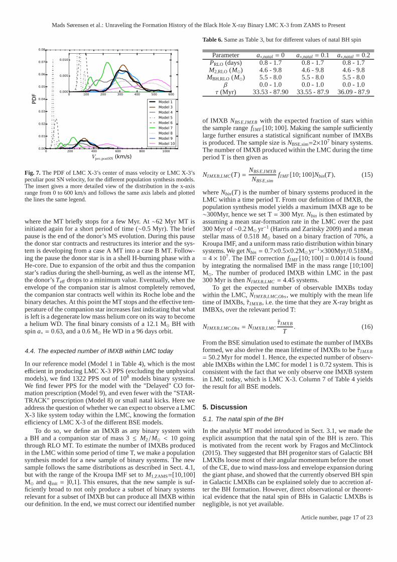
Mads Sørensen et al.: Unraveling the Formation History of the Black Hole X-ray Binary LMC X-3 from ZAMS to Present

0 200 400 600 800 1000

Vpec,postSN (km/s)

0.00

0.01

0.02

0.03

0.04

0.05

0.06

0.07

0.08

PDF

Model 1

Model 3

Model 4

Model 5

Model 6

Model 7

Model 8

Model 9

Model 10

0 100 200 300 400 500 6000.000

0.005

0.010

Fig. 7. The PDF of LMC X-3’s center of mass velocity or LMC X-3’speculiar post SN velocity, for the different population synthesis models.The insert gives a more detailed view of the distribution in the x-axisrange from 0 to 600 km/s and follows the same axis labels and plottedthe lines the same legend.

where the MT briefly stops for a few Myr. At∼62 Myr MT isinitiated again for a short period of time (∼0.5 Myr). The briefpause is the end of the donor’s MS evolution. During this pausethe donor star contracts and restructures its interior and the sys-tem is developing from a case A MT into a case B MT. Follow-ing the pause the donor star is in a shell H-burning phase withaHe-core. Due to expansion of the orbit and thus the companionstar’s radius during the shell-burning, as well as the intense MT,the donor’sTeff drops to a minimum value. Eventually, when theenvelope of the companion star is almost completely removed,the companion star contracts well within its Roche lobe and thebinary detaches. At this point the MT stops and the effective tem-perature of the companion star increases fast indicating that whatis left is a degenerate low mass helium core on its way to becomea helium WD. The final binary consists of a 12.1 M⊙ BH withspina∗ = 0.63, and a 0.6 M⊙ He WD in a 96 days orbit.

4.4. The expected number of IMXB within LMC today

In our reference model (Model 1 in Table 4), which is the mostefficient in producing LMC X-3 PPS (excluding the unphysicalmodels), we find 1322 PPS out of 108 models binary systems.We find fewer PPS for the model with the "Delayed" CO for-mation prescription (Model 9), and even fewer with the "STAR-TRACK" prescription (Model 8) or small natal kicks. Here weaddress the question of whether we can expect to observe a LMCX-3 like system today within the LMC, knowing the formationefficiency of LMC X-3 of the different BSE models.

To do so, we define an IMXB as any binary system witha BH and a companion star of mass 3≤ M2/M⊙ < 10 goingthrough RLO MT. To estimate the number of IMXBs producedin the LMC within some period of time T, we make a populationsynthesis model for a new sample of binary systems. The newsample follows the same distributions as described in Sect.4.1,but with the range of the Kroupa IMF set toM1,ZAMS=[10,100]M⊙ andqinit = ]0,1]. This ensures, that the new sample is suf-ficiently broad to not only produce a subset of binary systemsrelevant for a subset of IMXB but can produce all IMXB withinour definition. In the end, we must correct our identified number

Table 6. Same as Table 3, but for different values of natal BH spin

Parameter a∗,natal = 0 a∗,natal = 0.1 a∗,natal = 0.2PRLO (days) 0.8 - 1.7 0.8 - 1.7 0.8 - 1.7M2,RLO (M⊙) 4.6 - 9.8 4.6 - 9.8 4.6 - 9.8

MBH,RLO (M⊙) 5.5 - 8.0 5.5 - 8.0 5.5 - 8.0β 0.0 - 1.0 0.0 - 1.0 0.0 - 1.0

τ (Myr) 33.53 - 87.90 33.55 - 87.9 36.09 - 87.9

of IMXB NBS E,IMXB with the expected fraction of stars withinthe sample rangefIMF [10; 100]. Making the sample sufficientlylarge further ensures a statistical significant number of IMXBsis produced. The sample size isNBSE,sim=2×107 binary systems.The number of IMXB produced within the LMC during the timeperiod T is then given as

NIMXB,LMC(T ) =NBS E,IMXB

NBS E,simfIMF [10; 100]Nbin(T ), (15)

whereNbin(T ) is the number of binary systems produced in theLMC within a time period T. From our definition of IMXB, thepopulation synthesis model yields a maximum IMXB age to be∼300Myr, hence we set T= 300 Myr. Nbin is then estimated byassuming a mean star-formation rate in the LMC over the past300 Myr of∼0.2 M⊙ yr−1 (Harris and Zaritsky 2009) and a meanstellar mass of 0.518M⊙ based on a binary fraction of 70%, aKroupa IMF, and a uniform mass ratio distribution within binarysystems. We getNbin = 0.7×0.5×0.2M⊙ yr−1×300Myr/0.518M⊙= 4× 107. The IMF correctionfIMF [10; 100]= 0.0014 is foundby integrating the normalised IMF in the mass range [10;100]M⊙. The number of produced IMXB within LMC in the past300 Myr is thenNIMXB,LMC = 4.45 systems.

To get the expected number of observable IMXBs todaywithin the LMC, NIMXB,LMC,Obs, we multiply with the mean lifetime of IMXBs, τIMXB, i.e. the time that they are X-ray bright asIMBXs, over the relevant period T:

NIMXB,LMC,Obs = NIMXB,LMCτIMXB

T. (16)

From the BSE simulation used to estimate the number of IMXBsformed, we also derive the mean lifetime of IMXBs to be ˜τIMXB

= 50.2 Myr for model 1. Hence, the expected number of observ-able IMXBs within the LMC for model 1 is 0.72 system. This isconsistent with the fact that we only observe one IMXB systemin LMC today, which is LMC X-3. Column 7 of Table 4 yieldsthe result for all BSE models.

5. Discussion

5.1. The natal spin of the BH

In the analytic MT model introduced in Sect. 3.1, we made theexplicit assumption that the natal spin of the BH is zero. Thisis motivated from the recent work by Fragos and McClintock(2015). They suggested that BH progenitor stars of GalacticBHLMXBs loose most of their angular momentum before the onsetof the CE, due to wind mass-loss and envelope expansion duringthe giant phase, and showed that the currently observed BH spinin Galactic LMXBs can be explained solely due to accretion af-ter the BH formation. However, direct observational or theoret-ical evidence that the natal spin of BHs in Galactic LMXBs isnegligible, is not yet available.

Article number, page 17 of 23

A&A proofs:manuscript no. m_LMC_x-3

0

1

2

3

4

5

log(Period) (days) a)

PBSE MBH,MESA M2,MESA PBSE PMESA eBSE eMESA a ∗,MESA Teff,BSE Teff,MESA

5

10

15

20

25

Mass (M

⊙)

b)

0.1

0.3

0.5

0.7

0.9

e

c)

0 1 2 3 4 5 6 7

3.8

4.0

4.2

4.4

4.6

log(Teff) (k)

d)

BH

7.2 7.6 8.0 8.4 8.8 10 20 30 40 50time (Myr)

58.8 59.2 59.6 60.0 60.4

0.1

0.3

0.5

0.7

0.9

a∗

62 64 66 68 70

Fig. 8. Illustration of the complete evolution, of a typical LMC X-3PPS from ZAMS to a double CO (BH+WD) binary. Panel a) shows theevolution of the orbital period in days on a logarithmic scale. Panel b) displays the evolution of the masses in the binarysystem; the primarystarM1 as a star and as a BH (black line), and the companion starM2 (blue line). The black star label indicates the time of BH formation. Panelc) shows the evolution of the system’s eccentricitye in yellow, while in red we show the BH spin parametersa∗. Panel d) shows the effectivetemperatureTeff of the donor star in a logarithmic scale. Data coming from BSEsimulation are shown as dashed lines, while data from MESA assolid lines. From table 1 we have added; in panel a) the observed orbital period as the green dotted line, in panel b) the 1σ and 2σ error of M2

andMBH centered on the observed values, in panel c) the red dotted line is the upper 2σ limit on the BH spin parameter, and in panel d) the 1-σ

and 2σ error of Teff. In general, there is a fine agreement between BSE and MESA at the moment of RLO, except for the age of the system atRLO onset. MESA calculations find that RLO onset occurs at time= 8.8 Myr, whereas BSE finds it to begin at time= 12.2 Myr. The reason forthe discrepancy is the differences in the micro physics, between BSE and MESA, and in particular in the stellar structure calculations. Here, forillustrative purposes, the MESA calculations are offset to the right by 2.4 Myr in order to generate a smooth transition in the figure. The star marksthe formation of the BH at∼8 Myr and the vertical dashed line marks the time∼42 Myr at which the system crosses the observed orbital period.

In the context of our analysis, the assumption of zero natalspin is in fact a conservative one. This is because we only re-quire the mass that the BH accretes from the onset of the RLOphase until its current state, does not spin up the BH to a valueof a∗ that is higher than two sigma above the observed value. Ifa non-zero natal BH spin is assumed, then the maximum amountthat the BH in LMC X-3 may have accreted after its formation isfurther constrained to a smaller value. This has as a direct effectthat the minimum allowed natal mass of the BH goes up, butshould in principle also narrow down the allowed range of allthe binary properties of the system at the onset of RLO. Table6shows how these ranges change for a choice of natal BH spin ofa∗,natal = 0.1 anda∗,natal = 0.2, relative to our standard assump-tion of zero natal spin. Given, however, that it remains an openquestion how exactly BH form and how the formation processmay affect their natal spin, we decided to adopt the most conser-vative, wider range of allowed RLO properties, that corresponds

to a natal BH spin ofa∗,natal = 0. As Table 6 shows, althorughindividual MT sequences may not qualify anymore as PPS, thereare close to no changes in the overall estimated ranges. Onlytheminimum present age of the system increases as the natal spinincreases and is barely noticeable fora∗ = 0.1. The minimumage increases, as the more massive donors in a small orbit willbegin their RLO early enough to spin up the BH above the al-lowed spin limit. Assuming no natal spin we find a total of 395MT sequences as PPS for LMC X-3, and for a natal spin of 0.1and 0.2 respectively 371 and 336 PPS. As a limiting case, wemay consider the BH spin to be entirely natal, hence accretiononto the BH would not be possible. This would be equivalent toour case of MT sequences withβ = 1.

Article number, page 18 of 23

Mads Sørensen et al.: Unraveling the Formation History of the Black Hole X-ray Binary LMC X-3 from ZAMS to Present

1017 1018 1019 1020

MBH (g/s)

10-23

10-22

10-21

10-20

10-19

10-18

10-17

10-16

dN/(NdMBH)

Steiner et. al. 2014b

Persistent

Transient

Orosz et. al. 2014

Fig. 9. Distribution of observationally determined instantaneous accre-tion rates onto the BH taken at different time (black), and distributionof long-term average BH accretion rates inferred from MT sequence,calculated with MESA, that successfully reproduce the observed char-acteristics of LMC X-3. The green curve corresponds to MT sequencesthat predict a transient XRB, while the red curve corresponds to per-sistent ones. The vertical black dashed line shows the critical accretionrate for the thermal disk instability model, given by eq. (13), for theobservationally inferred properties given in Table 1.

5.2. The X-ray flux of LMC X-3

In Fig. 9 we compare the accretion rates onto the BH as inferredfrom thewinning MESA MT sequence models from Sect. 3.4 tothe observed values from Steiner et al. (2014a). The black solidline is the distribution of the observed instantaneous accretionrates, while the green and the red lines correspond to the long-term average accretion rate estimates from transient and persis-tent MESA MT sequences, correspondingly. The black dashedvertical line is the critical accretion rate for the development ofthe disk thermal instability, given from eq. (13), using theob-served values of LMC X-3 from Table 1.

Overall, it is shown that the observed accretion rates covers alarger range where as the MT sequence models distributes them-selves with most likely accretion rates near the critical accretionrate given by eq. (13) for the observed properties of LMC X-3from Table 1. This is similar to what was shown in Fig. 2, wherethe three examples of MT sequences were close to the criticalaccretion rate. We should stress here that a direct comparison be-tween the observations and the model predictions is not possible.This is because the observed instantaneous accretion ratescovera baseline of∼ 10 yrs, while our modelled MT sequences yieldan average value over timescales of few 105 to several 106 yrsand do not include any potential short term fluctuations. Keepingthis in mind, the general agreement between our predictionsandthe data at hand are notable and suggest a positive affirmation ofour model. The fact that our MT calculations predict MT ratesin the transition region between transient and persistent sourcesprovides a natural explanation for the atypical X-ray variabilityof LMC X-3.

5.3. Mechanism of Compact Object Formation

Although we see quantitative differences between the threedifferent CO prescriptions, "Rapid", "Delayed", and "STAR-TRACK" as a SN mechanism to have produced LMC X-3 we

cannot on this basis make a global ruling between the three pre-scriptions. It is however evident that "STARTRACK" is not ableto reproduce a statistical significant set of PPS for LMC X-3.Both the "Rapid" and "Delayed" prescriptions produce compa-rable results. A relevant question to ask is how the three prescrip-tions perform in producing a population of IMXB as we did inSect. 4.4. The result of repeating the population synthesisstudy(Sect. 4.4) for IMXB in LMC using the "STARTRACK" pre-scription yields that 0.98 IMXB is currently observable withinthe LMC. The "Delayed" prescription yields a total of 0.73 sys-tems is currently observable. In conclusion all three prescriptionsgive a consistent number of IMXB in LMC relative to observa-tions. The same can be said for the other individual models intable 4 with varyingαce andσv.

5.4. Natal kicks and the orbit of LMC X-3 within the LMC

An interesting perspective to be drawn from our synthesis popu-lation study with BSE is the increase in the PPS number, as weincreaseσv of the assumed Maxwellian asymmetric kick distri-bution from 0 s−1 to 265kms−1. Few PPSs are found when nokick or just a small kick is imparted. By gradually increasing thekick to be imparted until it equals the NS kick distribution,weincrease the number of PPSs. Most noticeable is the jump whengoing fromσv=26.5 s−1 to σv=100 km s−1, where the numberof PPSs increases by a factor∼10. Although we do not have di-rect evidence, there is strong indication that LMC X-3 likely hasformed with a kick being imparted to it. Given the lack of pre-cise enough peculiar motion measurements of LMC X-3, whichwould allow us to put direct constraints on the natal kick that theBH received, our estimates are depended on the assumed modelfor the compact object formation. This is because the latterdic-tates the relation between the pre-SN mass of the BH progenitorand its natal BH mass, and hence the amount of mass lost duringSN. A high mass-loss during SN tends to result in wide post-SNorbits, for which in turn a large kick in the appropriate directionis required in order to keep the tight.

The estimated post SN peculiar velocity or systemic veloc-ity of the binary’s center of mass is also relatively high. Evenfor cases with zero or small kicks the systemic velocity is likelyabove 50 km s−1. This is due to the high mass loss from the pri-mary during the SN (see Figure 5). This relative large post SNsystem velocity opens a question which only a kinematic studyof the LMC X-3 within LMC could answer. Given the high sys-temic velocity the system potentially received, it should affectthe system’s orbit within the parent galaxy. So, how is this or-bit looking today? If one had sufficiently accurate measurementsof the systems 3-dimensional motion and knew the potential ofLMC, it could be tested whether LMC X-3 is in a normal or-bit, most likely suggesting a low kick and low systemic velocity.If instead LMC X-3 was found to have a peculiar orbit, it wouldsuggest that the system would have received a high kick and highsystemic velocity. Finally, if the LMC X-3 was in an extreme or-bit or perhaps even escaped the LMC it would indicate that theLMC X-3 received a very high kick. In this respect it might bepossible to constrain the lower or upper natal kick imparted.

For LMC X-3 only the radial velocity is measured with ac-curacy. If one look at observations of radial velocities, whichare somewhat survey dependent, they suggest a radial velocityof Vrad = 300-308 km s−1; see Table 1 in Orosz et al. (2014).Using the model of van der Marel et al. (2002) updated withthe numbers of van der Marel and Kallivayalil (2014), one canget the expected radial velocity of a system in the LMC. Thismodel gives for LMC X-3 an expected radial velocity of 244

Article number, page 19 of 23

A&A proofs:manuscript no. m_LMC_x-3

km s−1 which compared to actual observations yields a differ-ence of∼55km s−1 suggesting the LMC X-3 center of massrest frame is moving faster than its neighbouring stellar popu-lation even when accounting for a velocity dispersion of∼20kms−1 (van der Marel and Kallivayalil 2014). The proper motion ofLMC X-3 is µαcos(δ) = -2.7 mas yr−1 ± 24.4 andµdelta = 12.5± 24.4 mas/yr−1 (Smart and Nicastro 2014), which if translatedinto a 3d velocity yield uncertainties so high it cannot be used toconstrain the LMC X-3 past evolution.

5.5. LMC X-3: The young sibling of GRS 1915+105?

A comparison of our MT sequences from MESA to the GalacticLMXB GRS1915+105, which has the largest measured spin ofall LMXBs a∗ > 0.98;(McClintock et al. 2006), provides someinteresting insights. Overall GRS1915+105’s current propertiesare P= 33.85 days (Steeghs et al. 2013),MBH = 12.4± 2.0M⊙(Reid et al. 2014a),M2 = 0.52± 0.41M⊙ (McClintock 2016),donor’s spectral type K0III-K3II andTeff = 4766.5 ± 666.5 K(Harlaftis and Greiner 2004; Greiner et al. 2001; Gray 2008;Cox 2000).

For our comparison we reran LMC X-3’s winning MT se-quences withβ = 0, allowing the largest amount of mass trans-ferred as possible, and compared them to the parameters ofGRS 1915+105 at its current orbital period. For the massesMBH,M2, andTeff we accept models that are within 2σ at the observedorbital period. For the BH spin parameter we make no constraint.We find 11 MT sequence models that match GRS1915+105 pa-rameters and with BH spin in the range 0.76 to 0.86. Figure 10show the comparison of one MT sequence model (see legend forsettings at RLO onset). In the three panels are shownTeff, M2,MBH as a function of orbital period. The color bar shows the BHspin parameter, as the BH is accreting material. Once the colorthickens the properties of the MT sequence model are within 2σof GRS 1915+105’s currently observed properties. The evolu-tion of the system is initially similar to that described in sec-tion 3.3. The abrupt increase inTeff at the end of the evolutionis the formation of a WD. The similarity between the evolutionof LMC X-3, from our simulations, and GRS1915+105 indicatethat these two systems potentially have formed from similarpro-genitor binary systems. Finally, although winning MT sequencesfor LMC X-3 with β = 0 can reach BH spinsa∗ > 0.8, it is clearthat the combination of donor and BH masses at the onset ofRLO do not provide a large enough mass reservoir to spin upthe BH to an extreme spin. As shown in Fragos and McClintock(2015), the range of donor masses at RLO onset that are requiredin order to spin up the BH in GRS 1915+105 to a∗ > 0.98is slightly higher than our inferred range for LMC X-3. Re-laxing our assumption for negligible natal spin for the caseofGRS 1915+105 would yield a much larger overlap between thePPSs for the two systems. This on the other hand would indicatea different compact object formation process for the BHs in thetwo systems.

6. Conclusion

In a two part study, we have reconstructed the evolution of LMCX-3 from its current X-ray bright MT phase, back to when thesystem was at the ZAMS. In the first part we formulated an ana-lytic MT point-mass model for the XRB phase that includes bi-nary component mass and orbital angular momentum changes,as well as changes in the spin parameter of the BH. The ana-lytic MT point-mass model was used to initially limit the pos-sible parameter space of LMC X-3’s PPS at the moment of

RLO onset, for which we then did detailed numerical simula-tions with MESA. We computed a regular space grid of 3319MT sequences of which 395 are solutions of the RLO onset set-tings of LMC X-3, with 121 MT sequences predicting a transientXRB and 274 MT sequences predicting a persistent one. Fromour detailed MT sequences we found that LMC X-3’s currentMT rate is very close to the critical MT rate predicted by thethermal instability disk model, which defines the boundary be-tween a persistent and transient source. This could potentiallyexplain LMC X-3’s high X-ray variability along with the factthat the system has always been bright since its discovery.

We then used the range of solutions at RLO onset foundfrom MESA to match to a large set of binary population syn-thesis simulations done with BSE. We considered 10 differentmodels with BSE, and for each model we estimated the mostlikely range for PPSs of LMC X-3 at the ZAMS, just prior tothe SN, just after the SN, and at the onset of RLO onset. In ad-dition we recorded the natal kick imparted to the BH during theSN and the systemic velocity after the kick. Overall we find,at 95 % confidence across all models, that LMC X-3 began asa ZAMS binary with a primary of massM1,ZAMS = 22.4-31.0M⊙, a secondary atM2,ZAMS = 5.0-8.2 M⊙, an orbital period ofPZAMS = 2 000−400 000 days, and an eccentricityeZAMS ≥ 0.23.Just prior to the SN, the primary had a massM1,preSN= 11.1-18.0M⊙, with the secondary star largely unaffected, though it mighthave accreted some of the mass lost from the primary. FromZAMS to just prior to the SN, the orbit decreased to periods be-tween 0.6-1.7 days, andepreSN≤ 0.44. We do find systems withno natal kick imparted, but these are few, and it is much morelikely that the SN explosion imparted a large kick of 120 km s−1

or more. Following the SN, the system has a BH ofMpostSN=

6.4-8.2 M⊙ in an eccentric orbit. From the time just after the SNand until the RLO onset, the orbit is circularised and it has anorbital periodPRLO = 0.8-1.4 days.

Finally, we discussed the potential for LMC X-3’s evolutionto be similar to the much older Galactic LMXB GRS1915+105.We demonstrated how LMC X-3 will likely not build up anequally extreme spin, because the LMC X-3 system overall hastoo little mass to accumulate such an extreme spin through ac-cretion. Despite this, it is likely that GRS1915+105 was also anIMXB when its RLO began, and followed a similar evolutionstarting with a slightly higher mass companion star.

In summary, we have successfully traced the evolution ofLMC X-3 from a ZAMS binary system until its current state.Studying LMC X-3 and constraining its characteristics, espe-cially during the CO formation, is of great importance for theunderstanding of how BH IMXB form and evolve. From an ob-servational point of view, we also offer a likely explanation forthe high X-ray variability associated with LMC X-3, by estimat-ing the current, long-term average MT rate close to the boundarybetween transient vs. persistent behaviour. Our prediction thatthe system likely received a large natal kick and has a corre-spondingly large post SN peculiar velocity could be tested withsufficient kinematic data and a proper motion study.

Acknowledgements. This work was supported by the Swiss National ScienceFoundation (project number 200020-160119). M.S. is grateful for support fromthe Swiss National Science Foundation and to the StarPlan Center, Universityof Copenhagen where much of this work was performed. T.S. acknowledgessupport from the Ambizione Fellowship of the Swiss NationalScience Foun-dation (grant PZ00P2_148123). J.F.S. has been supported byNASA EinsteinFellowship grant PF5-160144. The computations were performed at Universityof Geneva on the Baobab cluster. All figures were made with thefree Pythonmodule Matplotlib(Hunter 2007).

Article number, page 20 of 23

Mads Sørensen et al.: Unraveling the Formation History of the Black Hole X-ray Binary LMC X-3 from ZAMS to Present

10 20 30

period (days)

4000

6000

8000

10000

12000

14000

16000

Teff (K)

a)

β=0.0, MBH=6.0, M2=4.6, Porb=1.7

10 20 30

period (days)

0.1

0.5

1.0

2.0

3.0

4.0

5.0

M2 (M

⊙)

b)

10 20 30 40 50 60 70 80 90 100

period (days)

6

7

8

9

10

11

12

13

14

15

16

MBH (M

⊙)

c)

>0.8 0.85 0.9 0.95 1.0

a ∗

Fig. 10. A winning MT sequences simulated with MESA from RLO onset (see legend for values) and onwards until the donor becomes a WD.In the three panels, the observed properties of the GalacticLMXB GRS 1915+105 are shown, indicated by the gray areas. The light and darkgray areas are centered on the observed value of GRS 1915+105 and each gray contrast span 1σ on each side, except forM2 where the lower 2σlimit is truncated at 0. The dashed vertical line is the observed orbital period of 33.85 days of GRS1915+105. The color demonstrates the BH spinparametera∗ which for GRS 1915+105 isa∗ > 0.98, and it shows the maximum spin to be below 0.9. The thickening of the color illuminatingthe MT seq in each panel indicates the part of the evolutionary track for which the model properties are within 2σ of the observed properties ofGRS 1915+105 (excluding the BH spin). The sudden spike seen in the top panel is the formation of a WD.

References

Antoniou, V. and Zezas, A. (2016). Star formation history and X-ray binarypopulations: the case of the Large Magellanic Cloud.Monthly Notices of theRoyal Astronomical Society, 459(1):528–553.

Antoniou, V., Zezas, A., Hatzidimitriou, D., and Kalogera,V. (2010). STARFORMATION HISTORY AND X-RAY BINARY POPULATIONS: THECASE OF THE SMALL MAGELLANIC CLOUD. The Astrophysical Jour-nal Letters, 716(2):L140–L145.

Belczynski, K., Bulik, T., Fryer, C. L., Ruiter, A., Valsecchi, F., Vink, J. S., andHurley, J. R. (2010). On the maximum mass of stellar black holes. TheAstrophysical Journal, 714(2):1217.

Bondi, H. (1952). On spherically symmetrical accretion.MNRAS, 112:195.Brocksopp, C., Groot, P., and Wilms, J. (2001). The optical long period of lmc

x-3. Monthly Notices of the Royal Astronomical Society, 328(1):139–146.Cowley, A., Crampton, D., Hutchings, J., Remillard, R., andPenfold, J. (1983).

Discovery of a massive unseen star in lmc x-3.The Astrophysical Journal,272:118–122.

Cowley, A., Schmidtke, P., Ebisawa, K., Makino, F., Remillard, R., Crampton,D., Hutchings, J., Kitamoto, S., and Treves, A. (1991). Discovery of a long-term periodic variation in lmc x-3.The Astrophysical Journal, 381:526–533.

Cowley, A. P. (1992). Evidence for black holes in stellar binary systems.Annualreview of astronomy and astrophysics, 30:287–310.

Cox, A. N. (2000).Allen’s astrophysical quantities. AIP Press, Springer.

Cui, W., Feng, Y. X., Zhang, S. N., Bautz, M. W., Garmire, G. P., and Schulz,N. S. (2002). A Chandra Spectroscopic Survey of Persistent Black Hole Can-didates.The Astrophysical Journal, 576(1):357–365.

Dosopoulou, F. and Kalogera, V. (2016a). Orbital evolutionof mass-transferringeccentric binary systems. i. phase-dependent evolution.arXiv preprintarXiv:1603.06592.

Dosopoulou, F. and Kalogera, V. (2016b). Orbital evolutionof mass-transferring eccentric binary systems. ii. secular evolution. arXiv preprintarXiv:1603.06593.

Dubus, G., Lasota, J.-P., Hameury, J.-M., and Charles, P. (1999). X-ray irradia-tion in low-mass binary systems.Monthly Notices of the Royal AstronomicalSociety, 303(1):139–147.

Fragos, T., Kalogera, V., Willems, B., Belczynski, K., Fabbiano, G., Brassington,N. J., Kim, D.-W., Angelini, L., Davies, R. L., Gallagher, J.S., King, A. R.,Pellegrini, S., Trinchieri, G., Zepf, S. E., and Zezas, A. (2009). TransientLow-mass X-ray Binary Populations in Elliptical Galaxies NGC 3379 andNGC 4278.ApJ, 702(2):L143–L147.

Fragos, T., Linden, T., Kalogera, V., and Sklias, P. (2015).On the Formation ofUltraluminous X-Ray Sources with Neutron Star Accretors: The Case of M82X-2. ApJ, 802(1):L5.

Fragos, T. and McClintock, J. E. (2015). The Origin of Black Hole Spin inGalactic Low-mass X-Ray Binaries.The Astrophysical Journal, 800(1):17.

Fragos, T., Tremmel, M., Rantsiou, E., and Belczynski, K. (2010). Black HoleSpin-Orbit Misalignment in Galactic X-ray Binaries.ApJ, 719(1):L79–L83.

Article number, page 21 of 23

A&A proofs:manuscript no. m_LMC_x-3

Frank, J., King, A., and Raine, D. (2002).Accretion power in astrophysics.Cambridge University Press.

Fryer, C. L., Belczynski, K., Wiktorowicz, G., Dominik, M.,Kalogera, V., andHolz, D. E. (2012). Compact remnant mass function: dependence on theexplosion mechanism and metallicity.The Astrophysical Journal, 749(1):91.

Gou, L., McClintock, J. E., Reid, M. J., Orosz, J. A., Steiner, J. F., Narayan, R.,Xiang, J., Remillard, R. A., Arnaud, K. A., and Davis, S. W. (2011). TheExtreme Spin of the Black Hole in Cygnus X-1.The Astrophysical Journal,742(2):85.

Gray, D. F. (2008). The Observation and Analysis of Stellar Photospheres.TheObservation and Analysis of Stellar Photospheres, by David F. Gray, Cam-bridge, UK: Cambridge University Press, 2008.

Greiner, J., Cuby, J. G., McCaughrean, M. J., Castro-Tirado, A. J., and Men-nickent, R. E. (2001). Identification of the donor in the X-ray binary GRS1915+105. Astronomy and Astrophysics, 373(3):L37–L40.

Harlaftis, E. T. and Greiner, J. (2004). The rotational broadening and the mass ofthe donor star of GRS 1915+105. Astronomy and Astrophysics, 414(2):L13–L16.

Harris, J. and Zaritsky, D. (2009). The star formation history of the large magel-lanic cloud.The Astronomical Journal, 138(5):1243.

Hobbs, G., Lorimer, D. R., Lyne, A. G., and Kramer, M. (2005).A statisticalstudy of 233 pulsar proper motions.Monthly Notices of the Royal Astronom-ical Society, 360(3):974–992.

Hunter, J. D. (2007). Matplotlib: A 2d graphics environment. Computing InScience & Engineering, 9(3):90–95.

Hurley, J. R., Pols, O. R., and Tout, C. A. (2000). Comprehensive analytic for-mulae for stellar evolution as a function of mass and metallicity. MNRAS,315(3):543–569.

Hurley, J. R., Tout, C. A., and Pols, O. R. (2002). Evolution of binary starsand the effect of tides on binary populations.Monthly Notices of the RoyalAstronomical Society, 329(4):897–928.

Ivanova, N. (2006). Low-Mass X-Ray Binaries with Pre-Main-Sequence Com-panions.The Astrophysical Journal, 653(2):L137–L140.

Jeans, J. (1919). The origin of binary systems.Monthly Notices of the RoyalAstronomical Society, 79:408.

Justham, S., Rappaport, S., and Podsiadlowski, P. (2006). Magnetic brakingof Ap/Bp stars: application to compact black-hole X-ray binaries. MNRAS,366(4):1415–1423.

Kalogera, V. (1996). Orbital characteristics of binary systems after asymmetricsupernova explosions.The Astrophysical Journal, 471(1):352.

Kippenhahn, R. and Weigert, A. (1967). Entwicklung in engendoppelsternsyste-men i. massenaustausch vor und nach beendigung des zentralen wasserstoff-brennens.Zeitschrift fur Astrophysik, 65:251.

Kroupa, P. (2001). On the variation of the initial mass function. MNRAS,322(2):231–246.

Leong, C., Kellogg, E., Gursky, H., Tananbaum, H., and Giacconi, R. (1971).X-ray emission from the magellanic clouds observed by uhuru. The Astro-physical Journal, 170:L67.

Li, X.-D. (2015). Formation of black hole low-mass X-ray binaries. New As-tronomy Reviews, 64:1–6.

Linden, T., Sepinsky, J. F., Kalogera, V., and Belczynski, K. (2009). ProbingElectron-Capture Supernovae: X-Ray Binaries in Starbursts. The Astrophysi-cal Journal, 699(2):1573–1577.

Loveridge, A. J., Van der Sluys, M., and Kalogera, V. (2011).Analytical expres-sions for the envelope binding energy of giants as a functionof basic stellarparameters.The Astrophysical Journal, 743(1):49.

Maeder, A. (2008).Physics, formation and evolution of rotating stars. SpringerScience & Business Media.

Mandel, I. (2015). Estimates of black-hole natal kick velocities from observa-tions of low-mass X-ray binaries.arXiv, page 3871.

Mazeh, T., Van Paradijs, J., Van den Heuvel, E., and Savonije, G. (1986). Thelower mass limit of the compact object in lmc x-3.Astronomy and Astro-physics, 157:113–115.

McClintock, J. (2016). private communication.McClintock, J. E., Narayan, R., and Steiner, J. F. (2013). Black hole spin via con-

tinuum fitting and the role of spin in powering transient jets. Space ScienceReviews, 1:73.

McClintock, J. E., Shafee, R., Narayan, R., Remillard, R. A., Davis, S. W., andLi, L.-X. (2006). The spin of the near-extreme kerr black hole grs 1915+ 105.The Astrophysical Journal, 652(1):518.

Miller-Jones, J. C. A., Jonker, P. G., Dhawan, V., Brisken, W., Rupen, M. P.,Nelemans, G., and Gallo, E. (2009a). THE FIRST ACCURATE PARALLAXDISTANCE TO A BLACK HOLE. The Astrophysical Journal, 706(2):L230–L234.

Miller-Jones, J. C. A., Jonker, P. G., Nelemans, G., Portegies Zwart, S., Dhawan,V., Brisken, W., Gallo, E., and Rupen, M. P. (2009b). The formation of theblack hole in the X-ray binary system V404 Cyg.Monthly Notices of theRoyal Astronomical Society, 394(3):1440–1448.

Mirabel, I., Dhawan, V., Mignani, R. P., Rodrigues, I., and Guglielmetti, F.(2001). A high-velocity black hole on a Galactic-halo orbitin the solar neigh-bourhood.Nature, 413(6):139–141.

Mirabel, I., Mignani, R., Rodrigues, I., Combi, J. A., Rodríguez, L. F., andGuglielmetti, F. (2002). The runaway black hole GRO J1655-40. A&A,395(2):595–599.

Moreno Méndez, E. (2011). The need for hypercritical accretion in massiveblack hole binaries with large Kerr parameters.MNRAS, 413(1):183–189.

Moreno Méndez, E., Brown, G. E., Lee, C.-H., and Park, I. H. (2008). TheCase for Hypercritical Accretion in M33 X-7.The Astrophysical Journal,689(1):L9–L12.

Moreno Méndez, E., Brown, G. E., Lee, C.-H., and Walter, F. M.(2011). Kerr Pa-rameters for Stellar Mass Black Holes and Their Consequences for Gamma-ray Bursts and Hypernovae.The Astrophysical Journal, 727(1):29.

Motta, S. E., Muñoz-Darias, T., Sanna, A., Fender, R., Belloni, T., and Stella,L. (2014). Black hole spin measurements through the relativistic precessionmodel: XTE J1550-564.Monthly Notices of the Royal Astronomical Society:Letters, 439(1):L65–L69.

Naoz, S., Fragos, T., Geller, A., Stephan, A. P., and Rasio, F. A. (2015). Forma-tion of Black Hole Low-Mass X-ray Binaries in Hierarchical Triple Systems.arXiv, page 2093.

Orosz, J. A., Steiner, J. F., McClintock, J. E., Buxton, M. M., Bailyn, C. D.,Steeghs, D., Guberman, A., and Torres, M. A. (2014). The massof the blackhole in lmc x-3.The Astrophysical Journal, 794(2):154.

Paxton, B., Bildsten, L., Dotter, A., Herwig, F., Lesaffre, P., and Timmes, F.(2011). Modules for experiments in stellar astrophysics (mesa). The Astro-physical Journal Supplement Series, 192(1):3.

Paxton, B., Cantiello, M., Arras, P., Bildsten, L., Brown, E. F., Dotter, A.,Mankovich, C., Montgomery, M., Stello, D., Timmes, F., et al. (2013). Mod-ules for experiments in stellar astrophysics (mesa): planets, oscillations, ro-tation, and massive stars.The Astrophysical Journal Supplement Series,208(1):4.

Paxton, B., Marchant, P., Schwab, J., Bauer, E. B., Bildsten, L., Cantiello, M.,Dessart, L., Farmer, R., Hu, H., Langer, N., Townsend, R. H. D., Townsley,D. M., and Timmes, F. X. (2015). Modules for Experiments in Stellar Astro-physics (MESA): Binaries, Pulsations, and Explosions.ApJS, 220(1):15.

Pietrzynski, G., Graczyk, D., Gieren, W., Thompson, I., Pilecki, B., Udalski, A.,Soszynski, I., Kozłowski, S., Konorski, P., Suchomska, K., et al.(2013). Aneclipsing-binary distance to the large magellanic cloud accurate to two percent.Nature, 495(7439):76–79.

Piran, T. and Shaviv, N. J. (2005). Origin of the Binary Pulsar J0737-3039B.Physical Review Letters, 94(5):051102.

Podsiadlowski, P., Dewi, J. D. M., Lesaffre, P., Miller, J. C., Newton, W. G., andStone, J. R. (2005). The double pulsar J0737-3039: testing the neutron starequation of state.MNRAS, 361(4):1243–1249.

Podsiadlowski, P., Langer, N., Poelarends, A. J. T., Rappaport, S., Heger, A., andPfahl, E. (2004). The Effects of Binary Evolution on the Dynamics of CoreCollapse and Neutron Star Kicks.The Astrophysical Journal, 612(2):1044–1051.

Podsiadlowski, P., Rappaport, S., and Han, Z. (2003). On theformation andevolution of black hole binaries.Monthly Notice of the Royal AstronomicalSociety, 341(2):385–404.

Podsiadlowski, P., Rappaport, S., and Pfahl, E. D. (2002). Evolutionary Se-quences for Low- and Intermediate-Mass X-Ray Binaries.The AstrophysicalJournal, 565(2):1107–1133.

Rapley, C. and Tuohy, I. (1974). X-ray observations of the large magellaniccloud by the copernicus satellite.The Astrophysical Journal, 191:L113.

Reid, M., McClintock, J., Steiner, J., Steeghs, D., Remillard, R., Dhawan, V.,and Narayan, R. (2014a). A parallax distance to the microquasar grs 1915+105 and a revised estimate of its black hole mass.The Astrophysical Journal,796(1):2.

Reid, M. J., McClintock, J. E., Steiner, J. F., Steeghs, D., Remillard, R. A.,Dhawan, V., and Narayan, R. (2014b). A Parallax Distance to the Micro-quasar GRS 1915+105 and a Revised Estimate of its Black Hole Mass.TheAstrophysical Journal, 796(1):2.

Remillard, R. A. and McClintock, J. E. (2006). X-ray properties of black-holebinaries.Annu. Rev. Astron. Astrophys, 44:49–92.

Repetto, S., Davies, M. B., and Sigurdsson, S. (2012). Investigating stellar-mass black hole kicks.Monthly Notices of the Royal Astronomical Society,425(4):2799–2809.

Repetto, S. and Nelemans, G. (2015). Constraining the formation of black holesin short-period black hole low-mass X-ray binaries.MNRAS, 453(3):3341–3355.

Reynolds, C. S. (2013). Measuring Black Hole Spin Using X-Ray ReflectionSpectroscopy.Space Science Reviews, 183(1-4):81–294.

Smart, R. L. and Nicastro, L. (2014). The initial Gaia sourcelist. Astronomy andAstrophysics, 570:A87.

Article number, page 22 of 23

Mads Sørensen et al.: Unraveling the Formation History of the Black Hole X-ray Binary LMC X-3 from ZAMS to Present

Soria, R., Wu, K., Page, M., and Sakelliou, I. (2001). Xmm-newton opticalmonitor observations of lmc x-3.Astronomy & Astrophysics, 365(1):L273–L276.

Steeghs, D., McClintock, J. E., Parsons, S. G., Reid, M. J., Littlefair, S., andDhillon, V. S. (2013). The Not-so-massive Black Hole in the MicroquasarGRS1915+105. The Astrophysical Journal, 768(2):185.

Steiner, J. F., McClintock, J. E., Orosz, J. A., Buxton, M. M., Bailyn, C. D.,Remillard, R. A., and Kara, E. (2014a). Modeling the optical-x-ray accretionlag in lmc x-3: Insights into black-hole accretion physics.The AstrophysicalJournal, 783(2):101.

Steiner, J. F., McClintock, J. E., Orosz, J. A., Buxton, M. M., Bailyn, C. D.,Remillard, R. A., and Kara, E. (2014b). Modeling the optical-x-ray accretionlag in lmc x-3: Insights into black-hole accretion physics.The AstrophysicalJournal, 783(2):101.

Steiner, J. F., McClintock, J. E., Orosz, J. A., Remillard, R. A., Bailyn, C. D.,Kolehmainen, M., and Straub, O. (2014c). The low-spin blackhole in lmcx-3. The Astrophysical Journal Letters, 793(2):L29.

Tauris, TM & van den Heuvel, E. (2006). Formation and evolution of compactstellar x-ray sources.Compact stellar X-ray sources, 1:623–665.

Thorne, K. S. (1974). Disk-accretion onto a black hole. ii. evolution of the hole.The Astrophysical Journal, 191:507–520.

Valsecchi, F., Glebbeek, E., Farr, W. M., Fragos, T., Willems, B., Orosz, J. A.,Liu, J., and Kalogera, V. (2010). Formation of the black-hole binary m33 x-7through mass exchange in a tight massive system.Nature, 468(7320):77–79.

van den Heuvel, E. P. J. (1994). Interacting binaries: topics in close binary evo-lution. 22. Saas-Fee Advanced Course of the Swiss Society for Astrophysicsand Astronomy: Interacting binaries, -1:263–474.

Van der Klis, M., Tjemkes, S., and Van Paradijs, J. (1983). Ubv photometry ofthe optical candidate for lmc x-3.Astronomy and Astrophysics, 126(1):265–268.

van der Marel, R. P., Alves, D. R., Hardy, E., and Suntzeff, N. B. (2002). Newunderstanding of large magellanic cloud structure, dynamics, and orbit fromcarbon star kinematics.The Astronomical Journal, 124(5):2639.

van der Marel, R. P. and Kallivayalil, N. (2014). Third-epoch Magellanic CloudProper Motions. II. The Large Magellanic Cloud Rotation Field in Three Di-mensions.The Astrophysical Journal, 781(2):121.

van Loon, J. T., Cioni, M. R. L., Zijlstra, A. A., and Loup, C. (2005). An empir-ical formula for the mass-loss rates of dust-enshrouded redsupergiants andoxygen-rich Asymptotic Giant Branch stars.Astronomy and Astrophysics,438(1):273–289.

Vink, J. S. and de Koter, A. (2005). On the metallicity dependence of Wolf-Rayetwinds. A&A, 442(2):587–596.

Vink, J. S., de Koter, A., and Lamers, H. J. G. L. M. (2001). Mass-loss predic-tions for O and B stars as a function of metallicity.A&A, 369:574–588.

Warren, P. and Penfold, J. (1975). Photometry of lmc x-ray candidates.MonthlyNotices of the Royal Astronomical Society, 172(1):41P–47P.

Willems, B., Henninger, M., Levin, T., Ivanova, N., Kalogera, V., McGhee, K.,Timmes, F., and Fryer, C. (2005). Understanding compact object formationand natal kicks. i. calculation methods and the case of gro j1655–40. TheAstrophysical Journal, 625(1):324.

Willems, B., Kaplan, J., Fragos, T., Kalogera, V., and Belczynski, K. (2006). For-mation and progenitor of PSR J0737-3039: New constraints onthe supernovaexplosion forming pulsar B.Physical Review D, 74(4):043003.

Wong, T.-W., Valsecchi, F., Ansari, A., Fragos, T., Glebbeek, E., Kalogera, V.,and McClintock, J. (2014). Understanding compact object formation andnatal kicks. iv. the case of ic 10 x-1.The Astrophysical Journal, 790:119.

Wong, T.-W., Valsecchi, F., Fragos, T., and Kalogera, V. (2012). Understandingcompact object formation and natal kicks. iii. the case of cygnus x-1. TheAstrophysical Journal, 747(2):111.

Article number, page 23 of 23