u.s. corn yield capacity and probability: estimation and forecasting with nonsymmetric disturbances

Agricultural & Applied Economics Association

U.S. Corn Yield Capacity and Probability: Estimation and Forecasting with NonsymmetricDisturbancesAuthor(s): Paul GallagherSource: North Central Journal of Agricultural Economics, Vol. 8, No. 1 (Jan., 1986), pp. 109-122Published by: Oxford University Press on behalf of Agricultural & Applied Economics AssociationStable URL: http://www.jstor.org/stable/1349086 .

Accessed: 23/06/2014 21:02

Your use of the JSTOR archive indicates your acceptance of the Terms & Conditions of Use, available at .http://www.jstor.org/page/info/about/policies/terms.jsp

.JSTOR is a not-for-profit service that helps scholars, researchers, and students discover, use, and build upon a wide range ofcontent in a trusted digital archive. We use information technology and tools to increase productivity and facilitate new formsof scholarship. For more information about JSTOR, please contact [email protected].

.

Agricultural & Applied Economics Association and Oxford University Press are collaborating with JSTOR todigitize, preserve and extend access to North Central Journal of Agricultural Economics.

http://www.jstor.org

This content downloaded from 91.229.229.49 on Mon, 23 Jun 2014 21:02:15 PMAll use subject to JSTOR Terms and Conditions

http://www.jstor.org/action/showPublisher?publisherCode=oup

http://www.jstor.org/action/showPublisher?publisherCode=aaea

http://www.jstor.org/stable/1349086?origin=JSTOR-pdf

http://www.jstor.org/page/info/about/policies/terms.jsp


U.S. CORN YIELD CAPACITY AND PROBABILITY: ESTIMATION AND FORECASTING WITH NONSYMMETRIC DISTURBANCES

Paul Gallagher

This article explores the hypothesis that National Average Corn yields are skewed with a relatively high chance of occasional low yields. Maximum likelihood estimates support this hypothesis. Revised forecasts which account for skewed corn yields feature point and interval forecasts that are positioned higher than forecasts based on symmetric distributions. More- over, the chance of very low corn yields dominates the chance that the revised interval forecast is not realized.

Introduction

Despite the importance of corn yield variability in forecasting and price analysis, the research record on the probability distribution of national yields is less than complete. It is plausible that National average corn yields are skewed: yield cannot exceed the biological potential of the plant, yet it can approach zero under blight or early frost. Also, corn producers are concentrated in one region which experience similar weather, and the central limit theorem guaranties normally distributed yields for large areas only if individual producer's outcomes are independent in space. Foote and Bean examined pre WWII data and concluded that U.S. corn yields are skewed with a high probability of extremely low yields. In contrast, a more recent study (Luttrell and Gilbert) failed to duplicate Foote and Bean's conclusion, but the authors do caution that their result may be due to the uneven adoption of new corn production technology.

Paul Gallagher is an Assistant Professor of Agricul- tural Economics at Kansas State University, Manhat- tan, Kansas. This is Contribution 85-70-J from the Kansas Agricultural Experiment Station, Manhattan. The helpful remarks of James P. Houck, Clifford Hil- dreth, Don Groover and anonymous reviewers are gratefully acknowledged. This paper is contribution #85-70-Jat the Kansas Agricultural Experimental Sta- tion.

This paper provides evidence that the U.S. corn yield distribution is skewed with an upper limit (capacity) on output and a good chance of occasional low yields. Failure to recognize this skewed yield distribution leads to underestimates of most likely yields and the chances of extremely low yields. There is also potential for understating the importance of weather-related events in the United States, unless one accounts for rising corn yield variability associated with the technical changes of the past four decades.

The paper is organized in the following manner. In the first section, capacity yield is defined for a typical field crop, the reasons for deviations from capacity are considered, and plausible shapes of the probability distribution reflecting weather-induced variations in U.S. average corn yields are discussed. Then an estimation method which accounts for the capacity limitation and allows for nonsymmetric disturbances is presented. Subsequent results include an analysis of the effects of technical change on corn yield variability. Finally, prescriptions for forecasting deviations from capacity are proposed and forecasts based on skewed corn yield estimates are compared to standard forecasts based on normal disturbances.

The Concept of Capacity and Implications for Probability Distributions of Corn Yields

The notion that there is an upper limit on output lies at the heart of the capacity concept. Previous studies of industrial production have argued for an upper limit on the output obtainable with given technology and inputs by appealing to the "frontier" concept of economic theory (Forsund, et al.). In agricultural processes, however, the inten- sively used weather input fluctuates uncon- trollably. Consequently, the capacity concept should build on the notion that the full yield



110 NORTH CENTRAL JOURNAL OF AGRICULTURAL ECONOMICS, Vol. 8, No. 1, January 1986

potential of a crop is realized only with a particular combination of weather events. Capacity is defined here as the yield that would occur with (1) efficient use of the given technology for controllable inputs and (2) ideal weather.

Under the presumption that at least some dimensions of the weather input can be measured, the shape of the probability distribution of yield deviations from capacity can be analyzed in terms of the distribution of weather events and the relation between weather and corn yields. In particular, Foote and Bean first noted that the shape of corn yield distributions should depend on the probability distribution of the weather input and yield response to weather. In concluding an investigation of pre-war corn yields, they stated,

"Corn yields appear to be highly skewed. Extremely low values occur fairly frequently, but high yields are generally not much above the class interval that contains the highest frequency. This indicates that, in these areas, weather conditions generally are either close to op- timum or that some unfavorable factors are almost always present. Oc- casionally, however, conditions are such that yields are cut very ma- terially."

A subsequent empirical study of corn yields in several corn belt states verified the importance of diminishing and decreasing returns to weather inputs (Thompson). Several meteorological variables (e.g., monthly pre- cipitation, temperature) were stated as deviations about sample means. Statistical tests confirmed the necessity of using linear and (negative) quadratic terms to explain historical yield variation in these regions, which supports the notion of diminishing returns. Results also indicate that maximum yields occur near sample means for many independent variables thereby lending credibility to the hypothesis of decreasing returns.

The interaction between yield response to weather inputs and probability distributions of weather inputs is illustrated with a

one input example. Suppose weather can be measured by a single variable, Z, which represents rainfall by development stage of the plant or some other weighted average of rainfall. Furthermore, the possibility of diminishing and decreasing returns to weather inputs is represented by a quadratic relation between Z and crop yield (Y) in figure 1B. This rainfall-yield relation is defined by the conditions that (1) maximum yields of 130 bushels/acre occur when there is 5 inches of rainfall and (2) yields are zero when there is no rainfall. The position and shape of this function is defined by plant biology and the technology used in production. Thus, an increase in fertilizer application might increase the yield maximum and require more of the rainfall input.

An assumption about the probability distribution for Z is also necessary; a normal distribution illustrates that, even if the distribution of weather events is symmetric, the distribution of yield variation attributable to weather may be skewed and bounded by the rlants' potential with given technology and inputs. Three unit-variance rainfall distributions illustrate some climate possibilities (figure lA). The most-preferred of these three climates has a distribution whose mean rainfall is also the point of maximum yield: p=5.0. Climates that are generally too dry and too wet have means of p-2.0 and p-8.0, respectively. Notice that these inferior climates are both centered 3.0 rainfall inches away from the yield-maximizing level.

The normally distributed rainfall variable can be combined with the quadratic yield-rainfall relation to produce the implied probability distribution of crop yields. The yield density functions that result from this response curve and the alternative rainfall distributions are depicted in figure IC. The wet and dry climates each produce the same yield distribution because of symmetry. This yield distribution has a mode at 95 bu/acre, roughly 35 bushels below capacity. When the rainfall distribution is centered near the level that produces maximum yield, however, the probability distribution of deviations from capacity is monotonically declining.

While the argument above does not con- stitute proof that corn yields are negatively



CORN YIELD CAPACITY Gallagher 111

d 0.4

0.2

0 2.0 4.0 6.0 8.0 10.0 =2.0 it=5.0 p=8.0

Rainfall (inches)

(a) Unit Normal Rainfall Density Functions: g(Z) 1 exp[(Z-p)2 -F2r 2

120

100

80 -

60

40

20

0 2 4 6 8 10

Rainfall (inches) Z

(b) Rainfall-Yield Relationship: Y = 130 - 5.2 (Z-5)2

.040 -

Ideal Climate

0.30

C) .020 SToo Wet (t -2.0)

or Too Dry (i t=8.0)

.010 ,

20 40 60 80 100 120

Yield (bu./acre)- Y

(c) Yield Density Functions

Figure 1 A Comparison of Yield Probability Distributions with Alternative Distribu- tions of Rainfall.




skewed, empirical investigations are erected on plausible hypotheses. The example sug- gests a possibility that a corn yield distribution at one location is skewed giving an upper limit on output and a relatively good chance of occasional very low yields. Also, capacity yield may be most likely, but only if the distribution of weather events is centered near the yield maximizing level. Otherwise, the yield distribution is skewed and the mode is below capacity. However, the skewness properties of aggregate yields for large areas are dominated by effects that are common to all farms in a region, and so could be quite different from the skewness properties of yields on an individual farm. 1 Consequently, I agree with Day that a

"Supposition must not prejudice statistical analysis, for it is likely that the actual probability distributions vary significantly from crop to crop, from soil to soil, and from climate to climate... We must therefore accept evidence of asymmetry of whatever kind, and search for probability distributions of sufficient generality to describe any case that may arise in practice."

Estimation Methodology

Subsequent estimates build on the assumption that the composite of environmental effects on corn yields can be included in the disturbance term of a statistical model. 2 When the disturbance term is nonnormal and interest focuses on its shape, the usefulness of standard estimation methods diminishes. If the disturbance has constant variance, least squares still produces best linear unbiased (and consistent) estimates of regression parameters and traces a line through the mean of the skewed distribution (Kmenta, Green). Least squares estimates of residuals are not independent even when population disturbances are independent, however, so residuals are closer to the normal form than the actual error distribution (Huang and Bolch). Fortunately, maximum likelihood (ML) methods which build on the a priori no- tions of a limit on the dependent variable

and skewed disturbances have been developed (Green). Topics reviewed here include (1) a capacity function amenable to statistical analysis, (2) a functional form for the disturbance term, and (3) the execution and interpretation of maximum likelihood estimates.

Specifying a Capacity Function

Capacity estimates build on an algebraic approximation to the systematic and random influences on output. The yield potential or capacity of a crop is given by trend or more complex functions of technical and economic factors. Random fluctuations away from potential yield measure the environmental influence. It is assumed that the relation among observed yields (Yt), economic and technical factors (XI, ... . Xk), and the yield disturbance (Et), is linear:

Yt = a+1Xit+ ' ?

' +PfkXktEt

for t= 1,...,n, (1) where (a,#l, . . . , k) is a vector of parameters and (t > 0.

The Probability Distribution

The choice of a probability distribution requires a balance between conflicting criteria. First, the function should include varying degrees of skewness or even symmetry. Second, Green gives sufficient conditions for asymptotic properties of ML estimates; requirements that the density function and its derivative are both zero at the capacity point are among these conditions. Thus, the properties of ML estimators with the con- tinuously declining negative exponential distribution or with distributions without a tail near the origin are not known.

Estimates are based on the well-known Gamma distribution. This distribution is defined for a positive random variable E, and the density function can be expressed in terms of two parameters, 0 and a:

f(c ,a) a ,a-' exp [-Oc], E > 0. (2) T(a)




The Gamma distribution can be positively skewed or approach the symmetric normal distribution with appropriate parameter estimates. Using the difference between the mean and mode relative to the standard deviation as a skewness measure (Kendall and Stewart), it follows that skewness varies with the parameter a (figure 2).3 Asymptotic properties of ML estimation with the Gamma distribution are guaranteed provided that a >2 (Green, p. 41). This condition eliminates several highly skewed distributions. Howev- er, the qualitative conclusion of a highly skewed distribution is still warranted, even in the event that estimates in the region I < a < 2 are obtained. 4

Implementing the Maximum Likelihood Principle

The maximum likelihood principle prescribes a choice for the parameters of equations (1) and (2) which maximizes the log of the likelihood function.5 This problem eludes straightforward solution because the roots of the gradient vector (first derivatives of the log-likelihood function) are nonlinear functions of the parameters. Consequently, numerical analysis techniques, which search for the roots of the gradient, were employed (Dahlquist, Bjork and Anderson). The gradient method, which is stable but converges slowly, was first applied to initial estimates.

Thereafter, the rapidly-convergent Newton method was employed.6 Both methods were modified so that stepsize was defined by the highest likelihood function value in a given search direction. Also, individual gradient elements less than 10-5 indicated conver- gence.

Initial guesses are usually based on least squares estimates. When the population disturbance has constant variance, least squares estimates of e's and an intercept adjusted by the maximum positive residual provide consistent estimates of capacity function parameters (Green). As discussed subsequently, the variance of U.S. corn yields has been increasing, so estimations include an index of disturbance variability. Under these cir- cumstances, the bias in least squares estimates of capacity parameters is defined by the mean of the probability distribution of capacity deviations, and the correlation of independent variables with the variability of disturbances.7 Initial guesses are based on the estimated index of disturbance variability. For several assumed means of the capacity disturbance, bias-corrected capacity parameters and residuals were calculated from least squares estimates. Then, for each set of residuals, the maximum likelihood parameters and likelihood function for the Gamma distribution was calculated. The parameter set with the highest likelihood function was chosen as the initial guess.

S(a) 1.0

)E(c)

- M(c)_

1

0.8 r a

E(c): Mean 0.6 M(E): Mode

a: Standard 0.4 Deviation

0.2

0.0

0 4 8 12 16 20 24 28 32 36 40

Figure 2 Skewness Properties of the Gamma-distribution: the Mean/Mode Measure.




Analysis of U.S. Corn Yields

In addition to estimation procedures al- ready discussed, analysis of corn yields requires attention to several other factors. First, this study features a relatively long time series, which begins in 1933 and ends in 1981, and the U.S. corn industry provided the premiere example of yield increases attributable to new technology during this period. Consequently, a reasonable yield function for this historical period is discussed first. The specification accounts for technology and its uneven adoption. Furthermore, a yield function which measures the response to changing economic conditions is employed in this forecasting application. Thereafter, results which include the hypothesis that changes in technology and the location of corn production affect the variability of yields are presented. Then estimates are evaluated in prediction interval tests.

Capacity Function Specification

Misspecification of the effect of technical change may be at the root of opposing findings on the skewness of corn yields. Foote studied pre-WWII corn yields, a data set with no obvious trend in yields. He found negatively skewed yields. In contrast, Lut- trell and Gilbert used data from the 1930's to the 1970's and accounted for trend by re- gressing the logarithm of yields on time. They failed to find negatively skewed yields, but acknowledged that the trend in yields is misspecified.

In this study, the effect of technology was taken into account with a combination of trend and technique-specific methods. Two trend-regimes were identified on the basis of a preliminary examination of the yield series. The early part of the historical period (1933-55) was characterized by a gradual increase. The later period (1955-81) was first characterized by dramatic expansions, which tapered off during the 1970's. 8 Thus, a linear trend was specified for early years and logarithmic trend for the later years. Moreover, the equation was constrained so that the intercepts were equal

during the common year in both regimes (1955). Data on the adoption rate of hybrid seeds also was included as a technique- specific influence.

In conjunction, the adoption of hybrid seeds and conimmercial fertilizers probably in- troduced a fundamental change in the struc- ture of corn production relationships (Bray and Watkins). The hybrid seeds increased the plant's yield potential and response to soil fertility. In turn, commercial fertilizer turned a relatively fixed resource, soil fertility, into one whose application is readily con- trolled and, therefore, is subject to the profit-maximizing calculations of producers. Other research has confirmed that corn yields of the last three decades have been price responsive (Houck and Gallagher).

In specifying a yield function suitable for the period covering the adoption of hybrid seeds, it is useful to distinguish between those who adopted the new technique and those who did not. Suppose producers who use the traditional technique obtain yields that are represented as: ynh - nh nh nh

t nh t; nh represents a constant capacity and (nh describes random deviations from capacity for this group of producers. Producers adopting the new technology obtain yields that are governed by a price-responsive yield relationship:

yh = ah + hPth p th (**).

In both of the above equations, intercepts contain the impounded effects of other yield shifters.

The average yield for both groups of producers can be written conveniently with total production expressed as the sum of area planted to hybrid seeds (Ah) and area planted with traditional practices (Anh), each mul- tiplied by its appropriate Yield: QPt = AnhYnh + Ahyh. Note that total area (AT) is defined by this exhaustion classification: AT = Ah+Atnh. Then (national) average yields (YT) can be written as

yT - ytnh(lph+y hp (***),

where ph - Ath/A.




When (*) and (**) are substituted into equation (***), a composite yield response equation is obtained:

yr - ~anh + (aholLnh)p h + fh(p hpt)

- nh (-ph) + (thpth]

This relationship illustrates that the introduction of hybrids could influence yields by either of two mechanisms. The autonomous yield increase, represented by (ah-a nh)pth, indicates the increase in plant yield potential without additional treatment. The price responsiveness that occurs with the adoption of hybrids is represented by 3h(p 'Pt),

is attributable to a combination of price effect and new technique.

In the estimations that follow, lagged corn price relative to a fertilizer price index was taken as the supply-inducing price. Corn area planted is also an explanatory variable, included on the assumption that fertilizer de- cisions are made in the short-run. 9 An increase in a homogeneous land input generally reduces yield when the marginal product of land is less than the average product (Houck and Gallagher). Also, acreage control provi- sions for corn were initiated in 1938 and continued through the early 1970's (Cochrane and Ryan, pp. 133-4). Acreage controls provide an incentive to remove poor land from production first, so the acreage variable also serves as a proxy for the quality of land in production.

Heteroskedastic Corn Yields

The failure to consider heteroskedastic disturbance would be a possible specification error. For instance, variability increases associated with the passage of time and technology improvements have been proposed elsewhere (U.S. Department of Defense). More recently, increasing variability in U.S. corn yields has been documenlted and attri- buted to a narrowing genetic base (Hlazell). Moreover, corn production concentrated in midwestern states between the 1930's and early 1970's (Sundquist, et al.), then dispersed during the acreage expansions of

the last decade. A location shift to an in- creasingly sub-optimal area increases variability, if the response to weather inputs is higher in the sub-optimal areas.

The hypothesis of systematic changes in disturbance variance is tested with a procedure suggested by Glejser. In particular, the absolute value of least squares residuals are regressed against trend and planted area. The significance of explanatory variables provides a test of the heteroskedasticity hypothesis. Then an index of variability was calculated from the estimated absolute value of residuals defined by this regression. In turn, these corrections were used to obtain maximum likelihood estimates.

Preliminary Estimates

Experimentation involving technology specifications was conducted with least squares estimates. For example, three alternative views of the hybrid-yield relationship were considered. However, the intercorrela- tion between price and hybrid terms (R2=.92) precluded measurement of both effects together. Separately, the price effect or the autonomous effect was statistically significant and both relationships explained about the same proportion of historical variation (R2=.96). While either specification could be appropriate, subsequent results are based on the price effect in isolation. Also, the linear trend of the early regime, con- sistently insignificant in a variety of specifications, was discarded. In equation (3a) then, early yield expansions are explained by incentives for fertilizer use which occurred with the adoption of hybrid seeds and declining area planted. 10

YCPt=47.0949 + 9.9741CFRt

(10.06) (3.74)

- 0.2636ACP, + 68.2683TLOG (3a)

(.102) (3.39)

R2 = .9467 D.W. = 1.81 S = 5.523




Variable Definitions

YCTt: U.S. corn yield, bushels per planted acre

CFRt: HYBt x (PMCtI/PPFt) HYBt: Percent of corn acreage planted

with hybrid seeds (0-1) PMCt_I: Price received by farmers for corn

in previous year ($/bu) PPFt: Index of prices paid by farmers

for fertilizer (1910-1914=100) ACPt: U.S. corn acreage planted, in mil-

flons TLOG: LN(T)-LN(22); year > 55

IT=0 in 1933,..,22 in 1955,..49 in1981.

The trend adjustment (LN(22)) en- sures that the intercept for 1955 is the same as previous years.

The absolute value of residuals (ECt) from equation (3a) was used in the test of systematic changes in yield variability. The estimate below employs the segmented trend term (TLOG) as a measure of technological change. The percentage of U.S. corn area harvested in Illinois, Indiana, Iowa, and Ohio (PCBt) measures the location of production. The estimate below confirms the hypothesis of systematic changes in yield variability:

ECt 5.8593 - .1133PCBt

(3.76) (.108) + 8.9050TLOG, where R2 = 0.23 (3b)

An index of variability (VSt) was calculated from the estimated absolute value of residuals defined by equation (3b); a 1972 base year puts the reference point immediate- ly before the acreage expansions of the 1970's. Index values for recent years exceed the base year value by about 40 percent (Fig- ure 3).

Maximum Likelihood Estimates

The maximum likelihood result below is based on weighted values of the variables:

YCP, 1 CFRt vst,= 40.0367 + 9.2767

(4.35) t (1.17)VSt

ACP, TLOGt - .1236 +84.6605 (3c) (.044) VS (1.99) VS

Disturbance parameters:

0 = 0.2195, a = 2.6809

(.0474) (.5115)

100

80

60 Capacity

S40 .."-Actual S

20..... ...:: ,? 20

33 40 50 60 70 80

04I.2

-0.6

?0.2

33 40 50 60 70 80 Year

Figure 3 Corn Yields: Capacity and Actual (Left Scale), and Variability Index (Right Scale): 1933 to 1981.




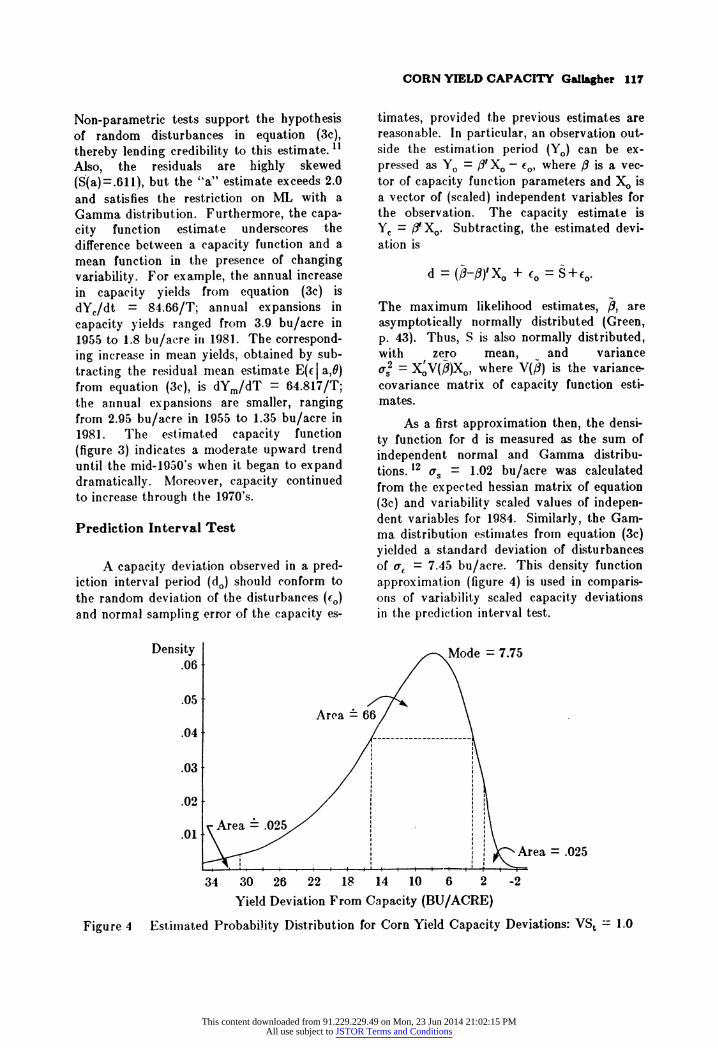
Non-parametric tests support the hypothesis of random disturbances in equation (3c), thereby lending credibility to this estimate. 11

Also, the residuals are highly skewed (S(a)=.611), but the "a" estimate exceeds 2.0 and satisfies the restriction on ML with a Gamma distribution. Furthermore, the capacity function estimate underscores the difference between a capacity function and a mean function in the presence of changing variability. For example, the annual increase in capacity yields from equation (3c) is dYc/dt = 84.66/T; annual expansions in capacity yields ranged from 3.9 bu/acre in 1955 to 1.8 bu/acre in 1981. The corresponding increase in mean yields, obtained by subtracting the residual mean estimate E( j a,0) from equation (3c), is dYm/dT = 64.817/T; the annual expansions are smaller, ranging from 2.95 bu/acre in 1955 to 1.35 bu/acre in 1981. The estimated capacity function (figure 3) indicates a moderate upward trend until the mid-1950's when it began to expand dramatically. Moreover, capacity continued to increase through the 1970's.

Prediction Interval Test

A capacity deviation observed in a prediction interval period (do) should conform to the random deviation of the disturbances (co) and normal sampling error of the capacity es-

timates, provided the previous estimates are reasonable. In particular, an observation outside the estimation period (Yo) can be expressed as Yo

= / Xo

- co, where f is a vec-

tor of capacity function parameters and Xo is a vector of (scaled) independent variables for the observation. The capacity estimate is

Yc = / Xo. Subtracting, the estimated deviation is

d = (3-1)'Xo + 0o = S+<.

The maximum likelihood estimates, /, are asymptotically normally distributed (Green, p. 43). Thus, S is also normally distributed, with zero mean, and variance a 2 - XoV(/)Xo,

where V(#) is the variance- covariance matrix of capacity function estimates.

As a first approximation then, the density function for d is measured as the sum of independent normal and Gamma distributions.12 as

= 1.02 bu/acre was calculated from the expected hessian matrix of equation (3c) and variability scaled values of independent variables for 1984. Similarly, the Gam- ma distribution estimates from equation (3c) yielded a standard deviation of disturbances of ac = 7.45 bu/acre. This density function approximation (figure 4) is used in comparis- ons of variability scaled capacity deviations in the prediction interval test.

Density Mode = 7.75 .06

.05 Area 66

.04

.03

.02

Area = .025 .01

Area = .025

34 30 26 22 18 14 10 6 2 -2 Yield Deviation From Capacity (BU/ACRE)

Figure 4 Estimated Probability Distribution for Corn Yield Capacity Deviations: VSt = 1.0




Table 1. Corn -- Actual Yields and Estimated Capacity Deviations Outside the Estimation Period

Year Capacity' Actual Deviation (Scaled)2 1982 103.5 100.6 2.9 (2.12) 1983 108.6 69.3 39.3 (27.31) 1984 109.5 95.2 14.4 (9.30)

1 Calculated with equation (3c). 2 Scaled deviations are actual deviations (column 4) divided by the index of variability (VSt) for the appropriate year. The values are VS8 = 1.376, VS8 = 1.44 and VS84 = 1.544.

Outlier identification is based on the ex- clusion of two and one-half percent probability from each tail of the distribution for d. Thus, scaled capacity deviations between 1.9 and 30.7 bushels per acre conform to the estimated density function for capacity deviations. From table I, the scaled capacity deviation was 2.12 bushels in 1982 and 27.3 bushels in 1984. Moreover, the 1983 deviation (9.3) is near the mode of the estimated density function. These observations sub- stantiate previous estimates of the capacity function and probability distribution.

Forecasting

The consequences of ignoring the skewed probability distribution for corn yield are a tendency to (1) underestimate most likely yield levels and (2) place an erroneous interpretation on the chance that a forecast is not realized. These points are made conveniently by comparing usual USDA procedures in making yield forecasts with revi- sions based on skewed distributions.

The USDA sometimes publishes yield forecasts at the beginning of each growing season which feature point estimates at the midpoint of a forecast interval which gives a two out of three chance that yield will fall within the interval (U.S. Department of Agri- culture). Furthermore, it is not unrealistic to assume that conventional methods are used in establishing these forecasts: the point esti-

mate represents a mean or regression line and confidence intervals are based on the normal distribution.

More general prescriptions for point and interval forecasts have been developed elsewhere. The forecasting rules are based on the premise that a point or interval should be chosen so that the highest probability possible is associated with the point or interval. Consequently, the mode of the distribution is the appropriate point estimate. In general, the end points of forecast intervals are defined by the requirements that (1) density function values are equal at interval end points and (2) the chance that the outcome is within the interval is given (Theil, 1965). These forecasting rules are based on a probability distribution that may be skewed. How- ever, they are equal to the standard procedures, with point estimates defined by regression lines and symmetric confidence intervals, when the yield distribution is symmetric.

A comparison of 1983 corn yield forecasts based on equation (3c) and a normal distribution with the same variance is shown in table 2. 1984 estimates of the capacity function provide the level for setting yield. The first row presents point estimates based on the mode and intervals calculated from the probability of success criteria. The second row contains point estimates based on the mean of the skewed distribution. Also, interval estimates are based on a normal dis-




Table 2. 1984 Corn Yield: Point and Interval Forecasts Based on Alternative Assump- tions About the Yield Error Distribution

Difference: Difference: Difference: Distribution Lower Lower to Point Point to Upper Lower to Assumption Limit3 Point Estimate Upper Limit3 Upper

-bushels per acre- Skewed' 86.0 15.8 101.8 2.7 104.5 18.5

(mode)

Symmetric2 79.0 11.6 90.6 11.6 102.2 23.2 (mean)

1984 Capacity Yield: 109.5

' These projections are based on the yield capacity estimate for 1984 corn yield and the probability distribution for capacity deviations discussed in the text. The point estimate for yield results from subtracting the mode of the error distribution from the 1984 capacity estimate.

2These projections are also based on the yield capacity estimate and the estimated density function. The point estimate results from subtracting the mean of the error distribution from the 1984 capacity estimate. The upper and lower limits are based on the estimated variance and the assumption that the distribution is normal.

3Upper and lower limits are calculated on the assumption of a 2-out-of-3 chance of actual yield to fall within these ranges.

tribution, with variance equal to that of the corresponding skewed distribution.

The point forecast based on the skewed distribution (101.8) is higher than the coun- terpart based on the normal distribution (90.6). Similarly, the interval for the skewed distribution (86.0 to 104.5) is positioned somewhat higher and is narrower than the corresponding interval for the normal distribution (79.0 to 102.2). Furthermore, most of the reduction in interval length occurs at the bottom of the forecast interval.

Conclusion

This study approached the problem of corn yield variability from the viewpoint that (1) plant biology and man's use of technology define an upper limit on output and (2) there is an asymmetrically high probability of occasional low yields.

There is evidence of skewed corn yields. Disturbance estimates were based on the

maximum likelihood method and the Gamma family of distributions -- the Gamma distribution may be highly skewed or approach the symmetric normal distribution. For corn yield disturbances over the 1933 to 1981 period, the best fit distribution was near the most skewed member of the Gamma family. The finding of negatively skewed corn yields is intertwined with measurements on the effect of technical change. An early period of gradual increases and a later period of more rapid increases in yields were identified. Further, yield functions based on this specification possessed random disturbances.

The implications of ignoring skewed corn yields are clear. In forecasting, point estimates are too low and intervals are positioned too low. Revised forecasts, which account for nonsymmietric distributions, feature forecast intervals that are positioned higher. Point estimates (model) lie above the midpoint of the interval and the chance of very low yields dominates the chance that the revised interval does not capture the actual




outcome. Similarly, evaluations of (1) the chances that public corn inventory schemes succeed or (2) the actuarial soundness of crop insurance that are based on normal distributions may misrepresent the desirability of these programs: the chances of extremely low yields and yields which are moderately above average will both be underestimated.

The analysis also demonstrates that capacity is a highly dynamic concept in the presence of technical change, as the variability of yields increases with the passage of time and the adoption of new technology. Because yield variability has increased with the passage of time, assessments of causes for corn price variability must acknowledge the increasing role played by weather related events in the United States.

References

Bray, James D. and Patricia Watkins, "Technical Change in Corn Production in the United States, 1870-1960." Journal of Farm Economics, November 1964: 751-65.

Cochrane, W. W. and M. E. Ryan, American Farm Policy, 1948-1973. Minneapolis: University of Minnesota Press, 1976.

Dahlquist, G., A. Bjork, and N. Anderson, Numerical Alethods. Englewood Cliffs, N.J.: Prentice-Hall, 1969.

Day, Richard H., "Probability Distribution of Field Crop Yields," Journal of Farm Economics 47 (1965): 713-741.

Foote, R. J. and L. Ii. Bean, "Are Yearly Variations in Crop Yields Really Random?" Agricultural Economics Research January (1957): 23-30. Forsund, F. R., C. A. Lovell and P. Schmidt, "A Survey of Frontier Productions and of their Relationship to Efficiency Measure- ment," Journal of Econometrics 13 (1980): 5- 25.

Glejser, H., "A New Test for Heteroskedasti- city," Journal of the American Statistical As- sociation 64 (1969): 316-23.

Green, W. H., "Maximum Likelihood Estima- tion of Econometric Frontier Functions," Journal of Econometrics 13 (1980): 27-56.

Hazell, P. B., "Sources of Increased Instabili- ty in Indian and U.S. Cereal Production," American Journal of Agricultural Economics 66 (1984): 302-11. Houck, J. P. and P. Gallagher, "The Price Responsiveness of U.S. Corn Yields," Ameri- can Journal of Agricultural Economics 58 (1976): 731-4.

Huang, C. J. and B. W. Bolch, "On Testing of Regression Disturbances for Normality," Journal of the American Statistical Associa- tion June (1974): 330-5.

Kendall, M. G. and A. Stuart, The Advanced Theory of Statistics - Volume I: Distribution Theory. New York: Hafner Publishing Com- pany, 1958.

Kmenta, J., Elements of Econometrics. New York: The Macmillan Company, 1971.

Luttrell, C. B. and R. A. Gilbert, "Crop Yields: Random, Cyclical or Bunchy?" American Journal of Agricultural Economics 58 (1976): 521-31.

Patel, J. K., C. H. Kapadia, and D. B. Owen, Handbook of Statistical Distributions. New York: Marcel Dekker, Inc., 1976.

Stevenson, R. E., "Likelihood Functions for Generalized Stochastic Frontier Estimation," Journal of Econometrics 13 (1980): 57-66.

Sundquist, W. Burt, K. M. Menz and Cather- ine F. Neumeyer, A Technology Assessment of Commercial Corn Production in the United States, University of Minnesota Agr. Exp. Sta. Bull. No. 546, 1982.

Theil, Henri, Economic Forecasts and Policy, Amsterdam: North-Holland Publishing Com- pany, 1965.

Thompson, L. M., "Weather and Technology in the Production of Corn in the U.S. Corn Belt." Agronomy Journal 61 (1969): 232-6.

U.S. Department of Agriculture, Economic Research Service, Feed Outlook and Situation Report. Washington, DC: FdS-296, May 1985.

U.S. Department of Defense, National De- fense University, Crop Yields and Climate Change to the Year 2000: Volume L. Wash- ington, DC, 1980.




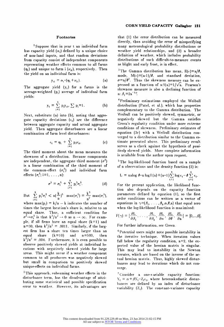
Footnotes

1Suppose that in year t an individual farm has capacity yield (ac) defined by a unique choice of non-land inputs, and that random deviations from capacity consist of independent components representing weather effects common to all farms

(rht) and unique to farm i (vit), respectively. Then

the yield on an individual farm is:

Yit = O,-(qt +vit). (a) The aggregate yield (Yt) for n farms is the acreage-weighted (p,) average of individual farm yields:

Yt =V PY,t, >_

pi=1. (b) i=1

Next, substitute (a) into (b), noting that aggregate capacity deviations

(t) are the difference

between aggregate capacity and actual aggregate yield. Then aggregate disturbances are a linear combination of farm level disturbances:

(t =- t - ,

Pivit. (c) i=1

The third moment about the mean measures the skewness of a distribution. Because components are independent, the aggregate third moment (a3) is a linear combination of the third moment of the common-effect (at3) and individual farm effects (a3; i=1, . .n):

3 = + A pi3O3 (d) i-1

But < n( )3 max(ai3) = - max(ao3), i=1 n 1 2

where max(pi) = k/n -- k indicates the number of times the largest location's share is, relative to an equal share. Thus, a sufficient condition for S 3--rt3 is that k3/n"

-- 0 as n -, oc. For exam-

ple, if all firms have an equal share (k=l) and n=30, then k3/n2 = .0011. Similarly, if the largest firm has a share ten times larger than an equal share (k=10) and n =500, then k3/n2 = .004. Furthermore, it is even possible to observe positively skewed yields at individual lo- cations with negatively skewed yields for large areas. This might occur if a weather component common to all producers was negatively skewed but small in comparison to positively skewed unique-effects on individual farms.

2This approach, subsuming weather effects in the disturbance term, has the disadvantage of attri- buting some statistical and possible specification error to weather. However, its advantages are

that (1) the error distribution can be measured directly, thus avoiding the error of misspecifying many meteorological probability distributions or weather yield relationships, and (2) a broader definition of weather, which includes probability distributions of such difficult-to-measure events as blight and early frost, is in effect.

3The Gamma distribution has mean, E(()=a/8, mode, M(c)=(a-I)/O, and standard deviation, a=a/02. Thus the skewness measure can be expressed as a function of a:S(a)=1/va. Pearson's skewness measure is also a declining function of a: /, =2a-'/2.

4 Preliminary estimations employed the Weibull distribution (Patel, et al.), which has properties complementary to the Gamma distribution. The Weibull can be positively skewed, symmetric, or negatively skewed but the Gamma satisfies Green's regularity condition under more extreme conditions of skewness. Preliminary estimates of equation (3c) with a Weibull distribution con- verged to a distribution similar to the Gamma estimate presented above. This preliminary result serves as a check against the hypothesis of positively skewed yields. More complete information is available from the author upon request. 5The log-likelihood function based on a sample of n observations and the density function (2) is:

n n

L = nalog 0-n log F(a) +(a-1) E log ,t- 8 N t. t=l t=1

For the present application, the likelihood function also depends on the capacity function parameters defined by equation (1), so the first order conditions can be written as a vector of equations in

y=(fl,..., ,k,a,O,a) that equal zero when the log-likelihood function is maximized:

[L aL, aL L OL F(1-) al[ , . l,

al," "i O ' I00' a []= 0,...,0].

For further information, see Green. 6 Potential users might note possible instability in the iterative technique. When iteration values fall below the regularity condition, a-2, the expected value of the hessian matrix is singular. This may lead to instability in the Newton iterates, which are based on the inverse of the actual hessian matrix. Thus, highly skewed disturbances may lead to iterations which do not con- verge.

7Consider a one-variable capacity function: Yt = a + /Xt-Zttt, where heteroskedastic disturbances are defined by an index of disturbance variability (Zt). The constant-variance capacity




disturbance ((t) can be related to a zero-mean disturbance (rzl) as: (t = /ap-rt,

where ,p+E(ft). Substituting yields a "mean" function: Yt =

a-ZP+fXt + Ztj. The least-squares slope

yixtYt ExtZt estimate is: = - - # - NxtZt .I

P + rijq.

There is bias in the least squares Ext2 estimate of # unless the capacity disturbance has constant variance (Zt--1) or if the variability index is uncorrelated with the independent variable (ExtZt=0):

'zJExtZt E() = , where x - Thus, an unbiased estimate of the capacity parameter is: c = Zx.

A similar but more complex argument can be made for a capacity model with several independent variables.

8This trend specification was the "best-fit" obtained from a fairly general family of yield-trend relationships. Preliminary regressions considered a yield-trend specification of the form:

Yt = a:#T+(al +f#T+lIT2)Dt, where

Yt: corn yield, T=trend(l in 1933, ..., 49 in 1981),

0, if T<T* D

1, if T>T*

and it was assumed that the two trend lines in- tersect at point T*, so that al+ flT.+ IT,2 = 0.

The "best" trend specification was obtained by calculating regressions with several values of T. and choosing the one with the minimum sum of squared errors. This procedure could establish a variety of possible trend forms as the best fit.

For example, end point solutions would establish linear or quadratic trends. Alternatively, interior solutions for T* could approximate the exponential curve used by Luttrell and Gilbert, or suggest a dampening trend effect at the end of the historical period.

The best fit actually occurred when T. was placed at 1955 and this result produced a negative estimate of -1y. Further information is available from the author upon request.

I9n general, supply (yield) functions depend on input-output price ratios of variable inputs and quantities of fixed inputs. After land allocations to crops are established in the spring, acreage is a fixed input and fertilizer is a variable input. 1oNumbers in parentheses below coefficients are standard errors. " The Wald-Wolfowitz Z-statistic and Wallis- More Xp2 statistic are tests of randomness based on the signs of deviations about the median and the signs of first differences of a series, respectively (Day). Under the null hypothesis of randomness, Z has approximately a unit normal distribution of Xp2, is distributed 7/6 x a chi-squared random variable. These non-parametric analo- gues to the Durbin-Watson statistic were calculated for the residuals of equation (3c), yielding Z=1.219 and Xp2-1.5004. The critical values at 10% significance are ZC=1.65 and Xp2,c = 5.37. Thus, both tests fail to reject the hypothesis of randomness.

12The density function for the sum of a normal and Gamma random variable, expressed in terms of the parameters of the component functions, is given by Stevenson.



u.s. corn yield capacity and probability: estimation and forecasting with nonsymmetric disturbances

Documents