u.s. manufacturing and the importance of international trade: it's

Federal Reserve Bank of St. Louis REVIEW January/February 2013 27

U.S. Manufacturing and the Importance ofInternational Trade: It’s Not What You Think

Kevin L. Kliesen and John A. Tatom

T he public and economic commentators often gauge the strength of the U.S. economy bythe quantity of automobiles, airplanes, and other manufactured goods produced overany given period of time. This sentiment perhaps harkens back to the nation’s leadership

in the Second Industrial Revolution, when the mass production of consumer and industrialgoods flourished. This rapid growth spurred a migration in the workforce from the farm tothe factory. In the past 50 years, though, the share of the nation’s employees in manufacturinghas steadily declined. Just after World War II, employees in manufacturing represented slightlyless than half of the total number of employees in private industry. This share has since declinedto about 11 percent today. Manufacturing employment peaked in June 1979 at around 20 mil-lion and then fairly steadily declined to about 11 million in January 2010.

To the layperson, the increasingly smaller share of U.S. employees in manufacturing is acause for concern. In recent years, such concern may have been exacerbated by the large-scalemovement of domestic production of certain goods to lower-wage countries such as China orMexico. Affected industries that readily come to mind are textiles, furniture, and certain elec-tronic goods (e.g., televisions). The popular consensus is that manufacturing employment trendsreflect an absolute decline in manufacturing output and the notion that America no longer pro-

The public often gauges the strength of the U.S. economy by the performance of the manufacturing sector, especially by changes in manufacturing employment. When such employment declines, as hasbeen the trend for many years, it is often assumed to be evidence of the slow death of U.S. manufacturingand an associated rise in imports. This article outlines key trends in U.S. manufacturing, especially thestrong performance of manufacturing output and productivity, and their connection to both exports andimports. The authors use ordinary regression, causality, and cointegration analyses to provide empiricalevidence for the positive role of imports in boosting manufacturing output. Policies to bolster exportsat the expense of imports would significantly harm U.S. manufacturing. (JEL O4, F4, E3)

Federal Reserve Bank of St. Louis Review, January/February 2013, 95(1), pp. 27-49.

Kevin L. Kliesen is a business economist and research officer at the Federal Reserve Bank of St. Louis. John A. Tatom is president and chief executive officer of Thoroughbred Economics. The authors thank Linpeng Zheng and Lowell Ricketts for research assistance.

© 2013, The Federal Reserve Bank of St. Louis. The views expressed in this article are those of the author(s) and do not necessarily reflect theviews of the Federal Reserve System, the Board of Governors, or the regional Federal Reserve Banks. Articles may be reprinted, reproduced,published, distributed, displayed, and transmitted in their entirety if copyright notice, author name(s), and full citation are included. Abstracts,synopses, and other derivative works may be made only with prior written permission of the Federal Reserve Bank of St. Louis.

http://research.stlouisfed.org/econ/kliesen/

duces tangible goods.1 In this view, imports are bad because they represent the offshoring ofdomestic jobs and the death of U.S. manufacturing.

The most recent recession reinforced the death-of-manufacturing view for many analysts.Manufacturing employment peaked in December 2007 and fell by over 2 million jobs by January2010. Industrial production declined by about 21 percent during the recent recession (December2007 to June 2009, according to the National Bureau of Economic Research). This decreasewas much larger than in the average recession (6.7 percent). The recovery period has also beenunusual. Typically, deep recessions are followed by strong recoveries, but real gross domesticproduct (GDP) growth during the current recovery has been weaker than normal.2 Nonetheless,the manufacturing sector has enjoyed a fairly robust recovery. Exports have been a key factorfueling the strong recovery in manufacturing. Moreover, some anecdotal evidence has suggestedthat increasing costs overseas, such as in China, have spurred some manufacturers to returnpart of their foreign production to domestic facilities. This development has been termed“onshoring.”

Accordingly, many policymakers have advanced the idea that exports are one of the bestelixirs for the manufacturing sector.3 This notion seems perfectly reasonable, since slightly morethan 70 percent of U.S. exports are manufactured goods. However, the manufacturing sectoralso depends heavily on imported intermediate products.

This article outlines key trends in the U.S. manufacturing industry, especially the outstandingperformance of manufacturing output and productivity, and then discusses their connection tointernational trade, both exports and imports. In particular, one of our key messages is that,perhaps contrary to conventional wisdom, imports of manufactured goods are extremely impor-tant for the manufacturing sector. Specifically, imports of intermediate materials contribute sig-nificantly to the industry’s strong rate of productivity growth. Exports alone do not exert such apositive influence. Thus, any attempts to bolster exports at the expense of imports, including bylowering the value of the dollar, would significantly harm the U.S. manufacturing sector, thenation’s productivity, and ultimately, long-term living standards. In addition, the recent recession,recovery, and expansion reinforce the long-term evidence that (i) U.S. manufacturing continuesto expand robustly and (ii) the weakness in manufacturing employment reflects relatively rapidproductivity growth, not the slow death of manufacturing. The final section of the article pro-vides empirical support for the positive role of imports in boosting U.S. manufacturing output.

KEY CHARACTERISTICS OF THE U.S. ECONOMY AND THE MANUFACTURING SECTOR

As in most advanced economies, the service sector accounts for the largest share of outputand employment in the United States. However, key segments in the service sector dependimportantly on manufactured goods, especially those related to information processing. At thesame time, key innovations developed by firms in the manufacturing sector have been adoptedby service-sector firms, enabling them to achieve substantial gains in efficiency and productiv-ity. For example, research has found that big-box retailers such as Wal-Mart and Target haveimproved the nation’s productivity by significantly increasing the efficiency of the supply chain

Kliesen and Tatom

28 January/February 2013 Federal Reserve Bank of St. Louis REVIEW

from manufacturer to retailer.4 This supply chain revolution—termed “just in time” inventories—was started by Toyota, a large global manufacturer.

Each quarter, the U.S. Census Bureau surveys a subset of the nation’s manufacturing, mining,trade, and selected service industries. The results are reported in its Quarterly Financial Report(QFR). In the first quarter of 2012, the Census Bureau surveyed 7,856 manufacturing firms froman estimated population of 137,770 firms. Most people probably believe that the typical U.S.manufacturing firm is a large multinational conglomerate like Toyota, Boeing, or Caterpillar.And indeed, Figure 1 indicates that 87 percent of assets are held by firms with assets in excess of$1 billion; but these firms make up only 9.8 percent of the total number of manufacturing firms.On the other end of the spectrum, 3,509 (45 percent) of the sampled firms had assets of lessthan $10 million.5 For example, at the end of 2010, Boeing reported assets of nearly $69 billionon its consolidated balance sheet, while Caterpillar reported assets of $64 billion.6 In short, theU.S. manufacturing sector is much like the U.S. commercial banking sector. That is, very largefirms account for the lion’s share of assets, but there is a large number of very small firms thataccount for a small percentage of industry assets.

A second characteristic of the U.S. manufacturing sector is its inherent volatility comparedwith the provision of services. As seen in Figure 2, the four-quarter growth of production in themanufacturing sector typically increases much more during recoveries and expansions and fallsby much more during recessions. In fact, the most recent recession is unusual because of thedepth of the decline in manufacturing output (17.4 percent) and because it was the first time in50 years that real service output declined during a recession. Despite the huge drop in manufac-

Kliesen and Tatom


2

3

1

2

5

87

0 20 40 60 80 100

<$10M

$10 to $50M

$50 to $100M

$100 to $250M

$250M to $1B

>$1B

Percent of Total Number of Firms

Total Assets of Firms

Figure 1

Manufacturing Corporations by Asset Size

SOURCE: Bureau of the Census, Quarterly Financial Report, 2012:Q1.

Kliesen and Tatom


–20

–15

–10

–5

0

5

10

15

20

1960 1965 1970 1975 1980 1985 1990 1995 2000 2005 2010

Percent Change from 4 Quarters Earlier

Industrial Production

Real Services Output

Figure 2

Real Services Output and Manufacturing Industrial Production

NOTE: Shaded areas indicate recessions as dated by the National Bureau of Economic Research.

SOURCE: Department of Commerce (Bureau of Economic Analysis) and Board of Governors of the Federal Reserve System.

1.6

2.3

2.8

3.7

0

0.5

1.0

1.5

2.0

2.5

3.0

3.5

4.0

4.5

1987-1995 1996-2012

Nonfarm Business

Manufacturing

Percent Change at Annual Rates

Figure 3

Labor Productivity Growth (1987-1995, 1996-2012)

SOURCE: Bureau of Labor Statistics.

turing output in the most recent recession, its volatility has continued a decline that began in1983—a period known as the Great Moderation. Since 1983, the standard deviation of thegrowth of manufacturing output has averaged 4.9 percent, while the standard deviation of thegrowth of service output has averaged 1.2 percent. This absolute and relative volatility compareswith 6 percent and 1.4 percent, respectively, for the period from 1960 to 1983.

A third key characteristic of the manufacturing sector is its relatively high rate of labor pro-ductivity growth compared with all other nonfarm businesses. Figure 3 plots the annualizedgrowth rate of labor productivity in the manufacturing and nonfarm private business sectorsfor the 1987-95 and 1996-2012 periods. We choose 1995 as the breakpoint since there appearsto have been a trend break in the data stemming from the information and communicationstechnology revolution.7 Also, official labor productivity data for the manufacturing sector beginin 1987. From 1987 to 1995, labor productivity in the manufacturing sector advanced at a 2.8percent annual rate, 1.2 percentage points faster than in the whole private nonfarm business(NFB) sector.8 But since manufacturing is included within nonfarm business and there is noseparate breakpoint for services, the growth of labor productivity in the service sector was evenweaker than in the NFB sector.

Since 1995, productivity in both the manufacturing and private NFB sectors has increasedsignificantly. Still, labor productivity growth in the manufacturing sector (3.7 percent per year)continued to outstrip labor productivity growth in the overall private NFB sector (2.3 percentper year). Indeed, although it is not shown in Figure 3, labor productivity growth in the manu-facturing sector has increased at a 4.2 percent annual rate since the trough of the recent recessionin the second quarter of 2009. Meanwhile, labor productivity growth in the private NFB sectorhas slowed to around 1.7 percent per year.

The faster growth of labor productivity in the manufacturing sector relative to the NFB sec-tor has produced two key effects. First, as seen in Figure 4, the share of manufacturing employ-ment has steadily declined since 1939, except for a brief upswing during World War II, while theshare of payroll employment in the service sector has increased. For purposes of comparison,Figure 4 also plots the private-sector share of construction employment, the other major categoryshown. Despite the recent housing boom, the share of employment in the construction sectorhas been relatively constant over time.

The decline in manufacturing’s share of private payroll employment parallels the decline inagricultural employment.9 Smaller employment shares for both agriculture and manufacturingreflect the steady substitution of labor for capital over time and the relatively rapid rates of pro-ductivity growth in each sector. Figure 5 indicates that capital spending is strongly positivelyassociated with the growth of manufacturing output.10 Business expenditures on equipmentand software are not a key driver of increases in manufacturing output. Rather, the causalityappears to run from manufacturing output to business investment, so strong growth of capitalspending is generally seen as a signal of strong output growth. However, capital spending is notpassive in an economic sense. Importantly, economic theory suggests that output per hour (laborproductivity) is a function of a firm’s (or a nation’s) capital-to-labor (K-L) ratio.

The manufacturing industry has steadily increased its K-L ratio over time at a faster ratethan has the service sector. Figure 6 plots the K-L ratio in the nonfarm, nonmanufacturing andmanufacturing sectors since 1939. From 1948 to 1995, the K-L ratio increased at a 2.7 percent

Kliesen and Tatom


Kliesen and Tatom


R2 = 0.46

–20

–15

–10

–5

0

5

10

15

–20 –15 –10 –5 0 5 10 15 20 25

Percent Change, Annual Data (1974-2011)

E&S Fixed Private Investment

IP-Mfg

Figure 5

Growth of Manufacturing Production and Equipment and Software Investment

NOTE: E&S, equipment and software; IP-Mfg, industrial production index for manufacturing output.

SOURCE: Federal Reserve Board of Governors and Bureau of Economic Analysis.

0

10

20

30

40

50

60

70

80

90

1939 1947 1955 1963 1971 1979 1987 1995 2003 2011

Services

Manufacturing

Construction

Percent of Total Private Payrolls

Figure 4

Private Employment Shares in the Service-Producing and Manufacturing Sectors


Kliesen and Tatom


0

20

40

60

80

100

120

140

1939 1947 1955 1963 1971 1979 1987 1995 2003 2011

Nonfarm, Nonmanufacturing

Manufacturing

Index, 2005 = 100

Figure 6

Capital-to-Labor Ratios in the Manufacturing and the Nonfarm, Nonmanufacturing Sectors


13.5

9.5

15.2

12.0

15.2

14.8

0

4

8

12

16

20

Total Mining,Utilities, andConstruction

Manufacturing Trade OtherIndustries

High-Tech

Percent, Average of Years Indicated

Figure 7

Industry Rates of Return on Capital (1999-2010)

SOURCE: Bureau of Economic Analysis, 2011 and 2012.

annual rate in the manufacturing sector but by only about 1 percent in the nonfarm, nonmanu-facturing sector. Since 1995, the growth rate of the K-L ratio has increased in both sectors,although by a bit more in the manufacturing sector. Since 1995, the K-L ratio has increased at a3.2 percent annual rate in the manufacturing sector and at a 1.5 percent rate in the nonfarm,nonmanufacturing sector.

A declining share of labor input and robust growth of manufacturing output and productivitysuggest a relatively strong rate of return on capital in the manufacturing sector. Indeed, this iswhat the data show. The Bureau of Economic Analysis (BEA) has released annual rates of returnin nonfinancial industries since 1999. Figure 7 shows the average annual rates of return from1999 to 2010 for total nonfinancial industries and mining, utilities, and construction; manufac-turing; retail and wholesale trade; high-technology; and all other industries.11 As the figureshows, the rate of return on capital for manufacturing (15.2 percent per year) has exceeded thetotal nonfinancial industries (13.5 percent) by a sizable margin. Over this period, rates of returnin manufacturing have exceeded all industries except the Other Industries group, where the rateof return is the same.

INTERNATIONAL INFLUENCESManufactured durable and nondurable goods comprise the largest share of U.S. exports. In

1929, goods exports were nearly 90 percent of total exports; by 2011 they had declined to about71 percent. In 2011, goods exports were $2.1 trillion. Service exports were a little more than$600 billion; although up significantly over time, as a share of total exports, service exports arestill only about 30 percent of total exports.

The composition of goods exports has also changed over time. Since reaching a trough of25 percent in 1933, durable goods exports as a share of total exports rose on net over the nextseveral decades, reaching a peak of 52 percent in 2000 (Figure 8). Over that same period, non-durable goods exports as a share of total exports declined from 60 percent to less than 20 per-cent. Since 2000, however, the share of durable goods exports has declined to 43 percent of totalexports, but this share is still within the 40 to 50 percent range experienced over most of thepost-World War II period. By contrast, the share of nondurable goods exports has risen toabout 28 percent of total exports. As seen in Figure 8, exports of nondurable goods nearlyequaled the share of services exports in 2011. The increased share of nondurable exports hasbeen in industrial supplies and materials and agricultural products.

Since most goods exports are manufactured products, it seems reasonable to conclude—assome policymakers evidently have—that the health of the U.S. manufacturing sector depends toa significant extent on the global demand for manufactured goods and this, in turn, depends onchanges in the exchange rate. One key development in this regard in recent years has been thesignificant increase in U.S. manufactured goods exports to China. Since 1990, U.S. goodsexports to China have increased by more than 20-fold (Figure 9). In contrast, U.S. goodsexports to the rest of the world have increased a little more than threefold. However, the corre-lation between the growth of manufacturing output and real goods exports is essentially zero.Figure 10 indicates a statistically insignificant positive correlation, an R-squared value of 0.05from 1974 to 2011. Perhaps even more counterintuitive to some is the correlation between the

Kliesen and Tatom


Kliesen and Tatom


0

10

20

30

40

50

60

70

1929 1937 1945 1953 1961 1969 1977 1985 1993 2001 2009

DurablesNondurablesServices

Percent of Total Exports

Figure 8

U.S. Export Shares by Type

SOURCE: Bureau of Economic Analysis.

0

5

10

15

20

25

1990 1994 1998 2002 2006 2010

Index, 1990 = 1.0

Exports to Rest of World Excluding China

Exports to China

Figure 9

U.S. Export of Goods

SOURCE: Department of Commerce (Bureau of the Census) and Council of Economic Advisers.

growth of real manufacturing output and the real value of the U.S. trade-weighted dollar; asshown in Figure 11, it is also essentially zero with an R-squared value of 0.01.

Do Imports Matter More than Exports?

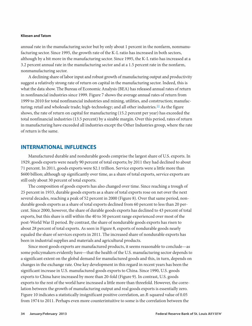
As noted previously, manufactured goods exports constitute the dominant share of U.S.exports. Moreover, exports of durable goods such as automobiles, construction equipment, orairplanes are the largest component of total U.S. exports. But what about imports? According tothe Boeing Company, non-U.S. suppliers provide roughly 30 percent of the content of its new787 Dreamliner.12 These include suppliers from Belgium, Canada, France, Italy, South Korea,the United Kingdom, and other countries.13 From this standpoint, then, imports are a key partof the manufacturing supply chain. Indeed, as shown in Figure 12, real goods imports have risenappreciably faster than real goods exports, as shares of manufacturing output. In 2011, the shareof real goods imports exceeded the share of real goods exports by about 34 percentage points.An increasing percentage of goods imports, perhaps not surprisingly, is from China and at theexpense of imports from other Pacific Rim countries, such as Japan. In 1992, the share of U.S.goods imports from China was about 5 percent and the share from other Pacific Rim countrieswas 34 percent. By 2011, China’s share had risen to 18 percent and the share of imports fromother Pacific Rim countries had declined to 14 percent. Not surprisingly then, the R-squaredvalue between the growth of manufacturing output and of real goods imports is exceptionallyhigh, 0.81 (Figure 13), and much stronger than that between the growth of manufacturing out-put and of real goods exports.

Kliesen and Tatom


–20 –10 0 10 20 30 40 50

R2 = 0.05

–20

–15

–10

–5

0

5

10

15


Real Goods Exports

IP-Mfg

Figure 10

Growth of Manufacturing Production and U.S. Real Goods Exports

NOTE: IP-Mfg, industrial production index for manufacturing output.


Kliesen and Tatom


R2 = 0.01

–20

–15

–10

–5

0

5

10

15

–15 –10 –5 0 5 10 15


Trade-Weighted Exchange Rate

IP-Mfg

Figure 11

Growth of Manufacturing Production and the Real Value of the U.S. Dollar


SOURCE: Federal Reserve Board of Governors.

0

20

40

60

80

100

120

1950 1956 1962 1968 1974 1980 1986 1992 1998 2004 2010

Exports

Imports

Percent

Figure 12

Real Goods Exports and Imports as a Percent of Real Manufacturing Value Added

SOURCE: Bureau of Economic Analysis.

Houseman et al. (2011) argue that manufacturing output and productivity have been affectedby “offshoring bias,” which provides an alternative reason for the strong correlation betweenimports and manufacturing output. Essentially, they argue that official statistics misstate pricedevelopments for intermediate materials that have moved from domestic production to foreignproduction. They show that prices of imports from developing countries have lower prices forintermediates than measured. Overstating the intermediary import prices tends to understatereal imports and thereby the contribution of imports to output. As a result, they argue, total fac-tor productivity, output, and labor productivity in manufacturing are biased upward. As long astrue real imports are positively correlated with measured imports, this bias imparts an upwardbias in the correlation between manufacturing output and imports. However, Houseman et al.estimate that the upward bias in output growth is 0.2 to 0.5 percentage points from 1997 to 2007,which is much smaller than the estimated contribution of imports to manufacturing outputgrowth estimated below. While their analysis has conceptual and theoretical significance, itspotential role in the story of the contribution of imports to manufacturing output here is minor.

FURTHER EMPIRICAL ANALYSISThe finding that the growth of manufacturing output is strongly correlated with goods

imports and not with goods exports is informative. It suggests that policies designed to restrictimports or artificially raise their costs would have adverse effects for U.S. manufacturers. Thus,if the trade-weighted value of the U.S. dollar were to decline, it is not definite that manufacturers

Kliesen and Tatom


R2 = 0.81

–20

–15

–10

–5

0

5

10

15

–20 –10 0 10 20 30


Real Goods Imports

IP-Mfg

Figure 13

Growth of Manufacturing Production and U.S. Real Goods Imports



would benefit to the extent that many believe.14 For example, a decline in the value of the dollarwould lower the price of U.S. manufactured goods to foreign buyers, which would increase U.S.goods and services exports, all else equal. At the same time, however, a weaker dollar would raisethe dollar price of imported goods and services in the United States. Thus, all else equal, Boeingwould pay more for imports of supplies and materials used to construct its 787 Dreamliner,which would increase the price of the Dreamliner, thereby reducing sales and therefore profits.

To formally test the hypothesis that imports matter as much as or more than exports to thegrowth of manufacturing output, this section presents the results of an ordinary least squaresregression analysis, a statistical test to assess causality, and an analysis of cointegration of manu-facturing output. In the regression analysis we model the quarterly growth of manufacturingoutput from 1973:Q2 to 2011:Q4.15 Our initial specification is that the growth (log change) ofreal manufacturing output is a function of the growth (log change) of (i) real GDP, (ii) foreignreal GDP, (iii) the real trade-weighted value of the U.S. dollar, (iv) real energy prices, (v) realgoods exports, and (vi) real goods imports. The specification also controls for the business cycleby including the first difference of the unemployment rate (vii) in the United States and (viii)abroad, although the latter was not statistically significant at a conventional 5 percent significancelevel and was dropped from the reported results. We also include a constant and a lagged valueof the dependent variable. We also examined lags of the independent variables, but none werestatistically significant.

In this specification, the coefficients on U.S. and foreign real GDP are expected to be positive;faster domestic and foreign growth would increase the demand for U.S. manufactured goods.The coefficients on real goods exports are also expected to be positive, because an increase ingoods exports is associated with increased foreign demand for U.S. manufactured goods.Although Figure 13 suggests that faster growth of real goods imports is associated with fastergrowth of real manufacturing output (a positive sign), it could also be true that faster growth ofreal goods imports reflects a substitution away from domestic manufactured goods. Thus, intheory, the sign could be negative.

The final three variables—the change in the U.S. unemployment rate, the real exchangerate, and real energy prices—are expected to have negative coefficients. A higher unemploymentrate generally indicates a slowing economy and thus weaker demand for U.S. manufacturedgoods. An appreciation of the dollar, for reasons noted previously, would also be expected toreduce the foreign demand for U.S. manufactured products. Finally, higher real oil prices notonly increase the price of manufactured goods (higher input costs and lower productivity), butthey also tend to reduce the growth rate of aggregate economic activity, which would also reducethe demand for manufactured goods.

Table 1 presents the results for our hypothesized specification. The first column shows theresults for the specification described above. Faster growth of domestic output (income), asexpected, raises the growth of manufacturing output, and the coefficient is relatively large (0.79)and statistically significant. Similarly, because a higher U.S. unemployment rate signals a slowerpace of economic activity, we anticipated that the coefficient for the change in unemploymentwould be negative; it is, and it is statistically significant. The growth of foreign output has a pos-itive and significant effect on domestic manufacturing output, as expected.

Kliesen and Tatom


We also hypothesized that the coefficient for the growth of real energy prices and the valueof the dollar would be negative. In each instance, however, the coefficient is positive, but verysmall. As Figure 11 shows, the coefficient for the change in the real value of the dollar is essen-tially zero and not significant. Similarly, the coefficient for growth of real energy prices is notstatistically significant at a conventional level. The final two independent variables for the firstmodel specification are the trade variables. Perhaps surprisingly, the growth of exports does nothelp to explain the growth of industrial production, as the coefficient is essentially zero and notsignificant. Hence, those who argue that enhancing U.S. goods exports should be a key strategyfor boosting the health of the manufacturing sector may be disappointed. However, goodsimports do appear to matter a great deal for the growth of manufacturing output. The coefficientis positive and highly significant, which must surprise critics of outsourcing, offshoring, andimports in general.

Table 1 reports two additional model specifications. The second specification drops theinsignificant real value of the dollar and export variables from the first specification; the energy

Kliesen and Tatom


Table 1

Predicting the Growth Rate of U.S. Manufacturing Output

Dependent variable: Log change of U.S. manufacturing output

Model specification

Independent variables (1) (2) (3)

Constant –1.49** –1.47** –1.53**(0.004) (0.004) (0.003)

Lagged dependent variable 0.10* 0.10* 0.11*(0.038) (0.039) (0.024)

U.S. real GDP 0.79** 0.78** 0.77**(0.000) (0.000) (0.000)

Foreign real GDP 0.35* 0.32* 0.38**(0.024) (0.029) (0.010)

Unemployment rate (%) –31.17** –31.22** –30.56**(0.000) (0.000) (0.000)

Real value of the dollar 0.01(0.692)

Real energy prices 0.02 0.02(0.062) (0.076)

Real imports 0.16** 0.16** 0.15**(0.000) (0.000) (0.000)

Real exports –0.01(0.664)

Adjusted R2 0.79 0.79 0.79

Durbin-Watson 1.93 1.95 1.96

Standard error of regression 3.36 3.34 3.37

NOTE: p-Values are listed in parentheses. The sample period is 1973:Q2 to 2011:Q4. * and ** indicate significance at the 5 percent and 1 percentlevels, respectively.

price variable is not significant, but since it is close to significance it is not dropped until thethird specification. In the second specification, the coefficients of the remaining variables areessentially the same, as is their significance and the fit of the equation. This is to be expected,given the small size and insignificance of the two omitted variables. In the third specificationwhere the real energy price measure is omitted, the results are essentially the same as in the sec-ond specification.

To summarize, we find some positive persistence in manufacturing output growth. We alsofind, perhaps not surprisingly, that domestic and foreign growth rates of real GDP matter sig-nificantly to the growth of manufacturing output, but the effect of the growth of U.S. output ismuch larger. This fact is reinforced by our finding that changes in the unemployment rate alsomatter significantly and negatively. Finally, we find, perhaps contrary to the conventional wisdom,that faster growth of U.S. exports does not seem to bear any relationship to the growth of U.S.manufacturing output. However, since the foreign demand for U.S.-produced goods probablydepends to a significant extent on the growth of foreign income and the price of U.S. manufac-tured goods, the export effect could be captured by the influence of the foreign output variable,which is highly significant. This could also explain why the real exchange rate is insignificant.

However, deleting foreign real GDP growth from the last two specifications in Table 1 (notshown) does not alter the significance of real export growth or, in the second specification, thegrowth of the real exchange rate. In the first specification, the coefficient on the growth rate ofexports, without the foreign real GDP variable, is 0.003 (p = 0.09) and for the growth rate of thereal exchange rate is 0.004 (p = 0.13). In the third specification, the coefficient on the growthrate of exports is 0.019 (p = 0.67). Thus, the results for the effect of real export growth, or thereal exchange rate, do not occur because of the correlation between export growth and foreignreal GDP growth.

Perhaps the biggest surprise to those who stress the importance of exports is the findingthat imports of manufactured goods seem to be much more important to the U.S. manufacturingsector. But why? Figure 14 helps to explain the answer. Eldridge and Harper (2010), workingwith BEA data, use a growth accounting exercise to estimate the contributions to manufacturingsector productivity growth from 1997 to 2006. Over this period, productivity growth averagednearly 4 percent per year. The contribution from multifactor (or total factor) productivityaccounted for a little less than half of this growth. Recall that multifactor productivity accountsfor changes in productivity not accounted for by capital and labor services. In a traditional growthaccounting model, intermediate inputs are not explicitly modeled. As a result, total output isequal to value added (real GDP originating).16

As seen in Figure 14, though, Eldridge and Harper (2010) also attempt to account for inter-mediate materials, those produced domestically and those imported from foreign sources. Theyfind that the combined contribution of intermediate materials to manufacturing productivitygrowth over this period was nearly 1.6 percentage points—almost as large as the contributionfrom multifactor productivity. But more interesting is their discovery that the contribution fromimported intermediate materials was slightly less than 1 percentage point, or nearly 50 percentlarger than domestically manufactured intermediate materials. According to Eldridge and Harper,in 1998 nearly 25 percent of intermediates used by the manufacturing sector was imported fromforeign sources; but, by 2006, this share had increased to 34 percent. This finding suggests that

Kliesen and Tatom


the value added from imported intermediates was proportionately much larger than that ofdomestic intermediates.

Houseman et al. (2011) argue that offshoring bias added 0.2 to 0.5 percent to real manufac-turing output growth over the 1997-2007 period. This amount is quite large, but the results inTable 1 suggest that the 6.25 percent import growth over the period contributed 1 percent tomanufacturing output growth over this period. Thus their results could account for about 20 to50 percent of the contribution of imports to real value added growth in manufacturing. This ispotentially a large effect, but one that still leaves a large role for the effect of imports on manu-facturing output.

From a policy perspective, the importance of intermediate materials to the U.S. manufactur-ing sector suggests that efforts to either restrict the flow of imports through quotas or raise theprice of intermediate materials through tariffs could harm the manufacturing sector. Similarly,to the extent that these intermediate materials are imported from Chinese sources, an apprecia-tion of the renminbi could similarly increase the cost for manufacturers and thus, all else equal,reduce manufacturing output.

Granger Causality Tests

The next issue is causality, which is examined using Granger causality tests. These testsassess whether past values of real import (or export) growth provide statistically significantexplanatory power for the current level of manufacturing output growth when previous values(lags) of manufacturing output growth are also included. If so, manufacturing output growth is

Kliesen and Tatom


3.96

1.79

0.64 0.650.92

0

0.5

1.0

1.5

2.0

2.5

3.0

3.5

4.0

4.5

Productivity MultifactorProductivity

CapitalIntensity

DomesticIntermediates

ImportedIntermediates

Productivity

Factor Contributions

Percent

Figure 14

Contributions of Nonlabor Factor Imputs to the Growth of Labor Productivity in the Manufacturing Sector(1997-2006)

SOURCE: Eldridge and Harper (2010).

said to be Granger-caused by real import (export) growth. It is possible that the regressionresult for imports in Table 1 could arise because of the effect of output growth on imports insteadof the effect of imports on output. A simple test of Granger causality shows that this is the case.The same is true for exports, even though they are not significant in Table 1.

Table 2 shows Granger causality test results for the growth rates of real imports and manu-facturing output and the growth rates of real exports and manufacturing output. For each pairof possible relationships—(i) export growth and manufacturing growth and (ii) import growthand manufacturing growth—lags of 8 or 4 past values of the growth rate of the dependent vari-able and the growth rate of the other variable are used to assess whether the other variable addsstatistically significant information.

For imports, the first two specifications in Table 2 (using 8 and 4 lags), the statistically sig-nificant F-statistic shows that the hypothesis that manufacturing output growth does not Granger-cause the growth rate of imports can be rejected. At the same time, the hypothesis that the growthrate of imports does not Granger-cause manufacturing output cannot be rejected. This test sug-gests that Granger causality runs in one direction—namely, from the growth of manufacturingoutput to the growth of imports. In other words, past manufacturing output growth helps toimprove the prediction of the current growth of real imports. The same is true for the growthrate of exports. The growth rate of exports does not Granger-cause manufacturing output, butthe growth rate of manufacturing output Granger-causes the growth rate of exports. Theseresults mean there is a strong, statistically significant temporal ordering. That is, accelerations

Kliesen and Tatom


Table 2

Granger Causality Testing for Statistical Causality Between the Growth of Goods Imports or Exports andthe Growth of Manufacturing Output

Granger causality test specifications F-statistic Probability

Import growth (GIMPORTS) and the growth of manufacturing output (IPMFG)

Lags: 8

IPMFG does not Granger-cause GIMPORTS 11.160 0.000

GIMPORTS does not Granger-cause IPMFG 0.942 0.484

Lags: 4

IPMFG does not Granger-cause GIMPORTS 21.680 0.000

GIMPORTS does not Granger-cause IPMFG 0.662 0.619

Export growth (GEXPORTS) and the growth of manufacturing output (IPMFG)

Lags: 8

IPMFG does not Granger-cause GEXPORTS 2.848 0.006

GEXPORTS does not Granger-cause IPMFG 1.163 0.327

Lags: 4

IPMFG does not Granger-cause GEXPORTS 5.253 0.001

GEXPORTS does not Granger-cause IPMFG 1.989 0.099

NOTE: The sample period is 1973:Q2 to 2011:Q4.

(decelerations) in manufacturing output growth precede significant increases (decreases) in bothimport and export growth. Attempts to restrict import growth are likely to weaken the growthof manufacturing output because of this linkage between the two measures.

Cointegration Test

A technical objection to regression analysis is the endogeneity of the independent variablesin Table 1, which in ordinary regression analysis should be independent of the dependent vari-able as well as each other. Table 2 supports causality from manufacturing output to imports, forexample. As indicated in the previous discussion, there are other interdependencies among thevariables. Stronger evidence of a long-run relationship between imports and manufacturingproduction is available from cointegration analysis. This approach also accommodates the endo-geneity problem. Cointegration analysis allows for mutual interdependence and determineswhether long-run relationships exist between measures in addition to the interdependencies.

The Johansen method of testing cointegration is used to test for cointegration betweenmanufacturing output and the significant variables in the last column of Table 1. Since the unem-ployment rate is a stationary variable, which means that it varies around a fixed mean over timeinstead of drifting over time (nonstationary), it is dropped from the potential cointegratingequation. All levels of the measures except the unemployment rate in Table 1 are found to benonstationary using unit root tests, but their first differences are stationary (not reported here).

None of the unit root tests for the variables has more than one significant lag; most have nosignificant lags. Therefore, two lags of the variables are included in the dynamic portion of thetest equations. Because none of the variables had a zero mean, the test equations include a con-stant in the cointegration equations. When all variables are included, the coefficient of mostmeasures in the potential cointegration equation is not significant. In particular, the natural

Kliesen and Tatom


Table 3

Cointegration Results for Manufacturing Output and Imports

Cointegrating equation

ln(XM)t – 0.401 ln(IM)t – 1.554 = et

(–21.03)

NOTE: The error term (e) is normally distributed with a zero mean and constant variance. It is the error correction term.

Models

dln(XM)t = –0.076 et–1 + 0.803 dln(XM)t–1 – 0.146 dln(XM)t–2 – 0.065 dln(IM)t–1 + 0.011 dln(IM)t–2 + 0.003

(–2.43) (7.93) (–1.23) (–1.19) (0.21) (1.99)

R2 = 0.42, SE = 0.014, SD (dependent variable) = 0.018.

dln(IM) = –0.040 et–1 + 1.633 dln(XM)t–1 – 0.639 dln(XM)t–2 – 0.125 dln(IM)t–1 + 0.061 dln(IM)t–2 + 0.010

(–0.71) (8.78) (–2.93) (–1.24) (0.64) (4.02)

R2 = 0.43, SE = 0.026, SD (dependent variable) = 0.034.

NOTE: Values in parentheses indicate t-statistics. XM, manufacturing output; IM, imports; SD, standard deviation; SE, standard error.

logarithms of manufacturing output (XM), exports (X), imports (IM), and foreign GDP (XF)were included in a preliminary estimate. Most of the variables in this cointegration equationestimate are not significant. The measure with the smallest t-statistic is foreign real GDP. A testfor restricting the coefficient on foreign real GDP to zero cannot be rejected (chi-squared statis-tic equals 0.61, insignificant at the 60.8 percent level), so it was dropped. The same insignificanceof most remaining coefficients in the cointegration equation still occurs, so the measure withthe smallest t-statistic, real GDP, was dropped next based on the same test of the restriction onits coefficient to equal zero (chi-squared statistic equals 0.95, insignificant at the 85 percentlevel). Finally, the export variable was dropped for the same reason (chi-squared statistic equals0.85, insignificant at the 85 percent level).

The resulting cointegration equation is shown in Table 3. The trace statistic for the hypothe-sis of no cointegration is 23.04, which rejects the hypothesis at the 2.02 percent significancelevel. Similarly, the maximum eigenvalue statistic of 16.30 rejects the absence of cointegration atthe 4.3 percent significance level. The cointegrating equation indicates that a 1-percentage-pointrise in imports is associated with a 0.4-percentage-point rise in manufacturing output in thelong run, much larger than shown in Table 1.

Kliesen and Tatom


Table 4

Impulse Response Estimates for Table 3

Response of manufacturing output Response of imports (XM) (IM)

Quarters XM IM XM IM

1 0.014 0.000 0.015 0.021

2 0.025 –0.001 0.037 0.019

3 0.029 –0.001 0.043 0.019

4 0.031 –0.001 0.043 0.020

5 0.031 0.000 0.043 0.020

6 0.031 0.000 0.042 0.021

7 0.031 0.000 0.041 0.021

8 0.030 0.000 0.040 0.021

9 0.030 0.000 0.040 0.022

10 0.030 0.000 0.039 0.022

11 0.029 0.001 0.038 0.023

12 0.029 0.001 0.038 0.023

13 0.029 0.001 0.037 0.023

14 0.029 0.001 0.036 0.024

15 0.028 0.001 0.036 0.024

16 0.028 0.001 0.035 0.024

17 0.028 0.001 0.035 0.025

18 0.028 0.002 0.034 0.025

19 0.027 0.002 0.033 0.026

20 0.027 0.002 0.033 0.026

An impulse response function shows the effect that a 1-standard deviation shock in onemeasure has on itself or another variable. Table 4 shows this for the estimates in Table 3. The“Response of manufacturing output (XM)” columns show the effects of a 1-standard deviationshock to manufacturing output and to imports on manufacturing output for the next 20 quarters.The “Response of imports (IM)” columns show the response of imports to a 1-standard deviationshock to manufacturing output and imports for the next 20 quarters. Entries in the table mustbe multiplied by 100 to obtain percentage-point effects. The first column in the table shows theeffect of a shock to manufacturing output on itself over the subsequent 5 years. The peak effectof the shock to manufacturing output on manufacturing growth occurs at five quarters whenoutput growth is boosted to 3.1 percent (100 × 0.031). Even after 5 years the effect persists,though it is declining. There is little effect on manufacturing output from a positive shock toimports for the next four quarters (second column). Subsequently, manufacturing output ishigher for the remainder of the 5 years, peaking at 0.2 percent after 20 quarters but still risingslowly toward its long-run effect. This confirms the conclusions in Tables 1 and 2 that a shockto imports will not reduce manufacturing output; instead, it boosts manufacturing output.

The response of imports to a positive shock to manufacturing output (third column) is pos-itive, relatively large, and it only returns to its long-run effect slowly. A shock to manufacturingoutput boosts imports by a peak rate of about 4.3 percent after four quarters, and the effectdeclines to about 3.3 percent after 5 years. The estimates show the strong effect of a positive shockto manufacturing output on imports. The effect of a 1-standard deviation shock to imports buildsslowly from 1 to 5 years later. At the end of 5 years, imports have been boosted by 2.6 percent.The dynamics in both cases show that imports and manufacturing output have a strong positiverelationship that persists for over 5 years, leaving a relatively large positive long-run effect.

The Johansen cointegration method is useful for testing for long-run relationships betweenvariables in a context where endogeneity exists among the variables. Its application here confirmsthe long-run positive relationship between manufacturing output and imports.

CONCLUSIONU.S. manufacturing suffered a massive decline during the recession in 2008-09, but it has

made an impressive comeback. Unfortunately, the same cannot be said for manufacturingemployment. Behind the recent trends is relatively rapid manufacturing productivity growth;this growth could have led to dramatic gains in output with unchanged employment, but manu-facturing demand is not as responsive to gains in income. The income gains from manufacturingproductivity growth boost demand for manufacturing output relatively less than the demandfor services. Thus, most of the gains appear in services output and employment with a relativelysmaller rise in manufacturing output. As a result, manufacturing employment is displaced toproduce services that are relatively more in demand as a result of manufacturing-led economicgrowth. The same phenomenon has characterized agricultural development for over a century.

In the 1980s, these developments were referred to as the “deindustrialization” of Americaand the “hollowing out” of the U.S. manufacturing industry. Much of the blame was laid on out-sourcing and offshoring to foreign subsidiaries and foreign firms. In fact, Tatom (1988) explainsthat the 1980s were characterized by a boom in manufacturing output and productivity that led

Kliesen and Tatom


economic growth in general and led demand for manufactured goods to outpace capacitygrowth in manufacturing. As a result, imports boomed along with domestic manufacturingoutput. The same has been true in the past decade. In recent years, the weakness of manufactur-ing employment, especially during the recession, has rekindled passions about the death ofmanufacturing. Continuing globalization has led critics to once again seize on internationalforces as both the culprit (imports) and the potential solution (increased exports) to the manu-facturing problem.

Several other trends in manufacturing continue to be important factors in understandingrecent developments. Manufacturing is dominated by some very large firms: Fewer than 10 per-cent of firms control almost 90 percent of manufacturing assets. Nonetheless, about 45 percentof the estimated 137,770 manufacturing firms have less than $10 million in assets. Output remainsvery volatile, especially in the durable goods sector where demand is readily postponed duringrecessions and resumed in expansions. This is less the case in nondurable manufacturing andusually barely noticeable in service industries.

The unusually strong performance of manufacturing productivity has largely been theresult of rising total factor productivity and relatively rapid growth in the capital-to-labor ratioin manufacturing. Both have accelerated since 1995 and increased even further in the latestrecession, recovery, and expansion. Evidence here also shows the expected positive link betweenstrong productivity growth, the relatively high real rates of return across the manufacturingsector, and the deepening of capital per worker or per labor hour.

Our analysis focuses on the role of exports and imports in affecting manufacturing per-formance. Surprisingly, we find that imports have played a critical positive role in boostingmanufacturing output in the United States—much more so, in fact, than exports. We find nodiscernible influence of export growth on manufacturing growth, but there is a strong positiveinfluence of import growth on manufacturing growth. Many industry, labor, and political leadersbelieve that boosting manufacturing growth will require limiting imports through favorablepreferences for domestic purchasing and raw material and capital goods sourcing, perhapsthrough quotas, tariffs, domestic content legislation, or simply discriminatory preferences.However, reliance on imports has been a strong positive influence on manufacturing outputand productivity. Moreover, there is no discernible gain to manufacturing growth that couldarise from new policies proposed to boost exports.

We present causality tests indicating that neither imports nor exports cause manufacturinggrowth. Instead, both exports and imports are led systematically by prior growth in manufac-turing. Thus in the recent recession, a large subsequent decline in imports and exports shouldnot have been a surprise. The importance of imports to domestic manufacturing performancecannot be overstated. Goods imports equal more than 100 percent of manufacturing value added,so they account for more than half of the gross output and sales of domestically produced prod-ucts. Intermediate goods imports and capital goods imports are the lifeblood of U.S. output.Exports account for a much smaller share of manufacturing value added. While development offoreign markets offers an opportunity for outsized growth, the success of manufacturing hasnot been as critically dependent on new markets for sales as for new markets for materials andcapital goods.

Kliesen and Tatom


NOTES1 Bartlett and Steele (2012) argue that government policy has been responsible for the decline in manufacturing. They

call for more protective actions to reduce imports of manufactured goods.

2 See Bordo and Haubrich (2012).

3 See chapter 5 of the 2012 Economic Report of the President, which discusses the Obama administration’s 2010National Export Initiative. The goal of this initiative is to double U.S. exports of goods and services from 2010 to 2015.

4 See the summary of a 2001 McKinsey Global Institute study at www.mckinsey.com/insights/mgi/research/productivity_competitiveness_and_growth/us_productivity_growth_1995-2000.

5 See Table N of the 2012:Q1 QFR.

6 Assets reported on the consolidated balance sheet. Values for Boeing and Caterpillar are derived from their companyForm 10-K annual reports to the Securities and Exchange Commission. Seewww.sec.gov/Archives/edgar/data/12927/000119312511028490/d10k.htm andwww.caterpillar.com/cda/files/2652288/7/2010+10K.pdf.

7 These issues are discussed in Anderson and Kliesen (2006).

8 These data are reported by the Bureau of Labor Statistics.

9 See Kliesen and Poole (2000).

10 Unless noted otherwise, manufacturing output in this article is measured by the index of industrial production forthe manufacturing sector. This series is calculated and published by the Board of Governors of the Federal ReserveSystem in its G.17 (Industrial Production and Capacity Utilization) statistical release.

11 According to the BEA, “other industries” consists of agriculture, forestry, fishing, and hunting; transportation andwarehousing; information; rental and leasing services and lessors of intangible assets; professional, scientific, andtechnical services; administrative and waste management services; educational services; health care and social assis-tance; arts, entertainment, and recreation; accommodation and food services; and other services, except govern-ment. See Hodge et al. (2011).

12 See the 787 Dreamliner Program Fact Sheet at www.boeing.com/commercial/787family/programfacts.html.

13 See the suppliers for the Dreamliner at www.airframer.com/aircraft_detail.html?model=B787.

14 Many analysts have pointed out the deficiencies of currency depreciation in improving current account imbalances.For example, see McKinnon (2005) and Tatom (2007).

15 See endnote 10. Much of the data for this analysis can be found in the St. Louis Fed’s FRED database:http://research.stlouisfed.org/fred2/.

16 See Anderson and Kliesen (2006) for a discussion.

REFERENCESAnderson, Richard G. and Kliesen, Kevin L. “The 1990s Acceleration in Labor Productivity: Causes and Measurement.”

Federal Reserve Bank of St. Louis Review, May/June 2006, 88(3) pp. 181-202; http://research.stlouisfed.org/publications/review/06/05/Anderson.pdf.

Bartlett, Donald L. and Steele, James B. The Betrayal of the American Dream. New York: PublicAffairs, 2012.

Bordo, Michael D. and Haubrich, Joseph G. “Deep Recessions, Fast Recoveries, and Financial Crises: Evidence from theAmerican Record.” Federal Reserve Bank of Cleveland Working Paper No. 12-14, June 2012;www.clevelandfed.org/research/workpaper/2012/wp1214.pdf.

Economic Report of the President. Washington, DC: United States Government Printing Office, 2012; www.whitehouse.gov/administration/eop/cea/economic-report-of-the-President.

Eldridge, Lucy P. and Harper, Michael J. “Effects of Imported Intermediate Inputs on Productivity.” Monthly LaborReview, June 2010, pp. 3-15; www.bls.gov/opub/mlr/2010/06/art1full.pdf.

Kliesen and Tatom


www.mckinsey.com/insights/mgi/research/productivity_competitiveness_and_growth/us_productivity_growth_1995-2000

www.mckinsey.com/insights/mgi/research/productivity_competitiveness_and_growth/us_productivity_growth_1995-2000

Hodge, Andrew W.; Corea, Robert J.; Green, James M. and Retus, Bonnie A. “Returns for Domestic NonfinancialBusiness.” Survey of Current Business, Bureau of Economic Analysis, June 2011, pp. 24-28;http://bea.gov/scb/pdf/2011/06%20June/0611_domestic.pdf.

Houseman, Susan; Kurz, Christopher; Lengermann, Paul and Benjamin Mandel. “Offshoring Bias in U.S. Manufacturing.”Journal of Economic Perspectives, 25(2) 2011, pp. 111-32;www.brmandel.com/uploads/3/2/4/5/3245755/jep.25.2.pdf.

Kliesen, Kevin L. and Poole, William. “Agricultural Outcomes and Monetary Policy Actions: Kissin’ Cousins?” FederalReserve Bank of St. Louis Review, May/June 2000, 82(3) pp. 1-12;http://research.stlouisfed.org/publications/review/00/05/05kk.pdf.

McKinnon, Ronald I. “Currency Wars.” Wall Street Journal, July 29, 2005;www.stanford.edu/~mckinnon/briefs/CurrencyWars.pdf.

Tatom, John A. “The Link Between the Value of the Dollar, U.S. Trade and Manufacturing Output: Some RecentEvidence.” Federal Reserve Bank of St. Louis Review, November/December 1988, pp. 24-37; http://research.stlouisfed.org/publications/review/88/11/Link_Nov_Dec1988.pdf.

Tatom, John A. “The US-China Currency Dispute: Is a Rise in the Yuan Necessary, Inevitable or Desirable?” GlobalEconomy Journal, 2007, 7(3), Article 2.

Kliesen and Tatom


u.s. manufacturing and the importance of international trade: it's

Documents