USE OF DVB-T AND DVB-S2 IN TELECARDIOLOGY

A THESIS SUBMITTED TO THE

GRADUATE SCHOOL OF APPLIED SCIENCES

OF

NEAR EAST UNIVERSITY

By

WALEED ALSAADI

In Partial Fulfillment of the Requirements for

the Degree of Master of Science

in

Electrical and Electronic Engineering

NICOSIA, 2015

ii

I hereby declare that all information in this document has been obtained and presented in

accordance with academic rules and ethical conduct. I also declare that, as required by these

rules and conduct, I have fully cited and referenced all material and results that are not original

to this work.

Name, last name: Waleed ALsaadi

Signature:

iii

ACKNOWLEDGMENTS

I truly feel very thankful to my supervisor Assist. Prof. Dr. Ali Serener for his assistance,

guidance and supervision of my thesis. I appreciate his continuous follow up, support and

motivation. He was always sharing his time and effort whenever I need him.

I acknowledge Assist. Prof. Dr. Kamil Dimililer for his understanding, supporting and being

always there for any advice.

I really feel very thankful to Prof. Dr. Rahib Abiyev for his great advices, enormous support

and helping me to enrich my thesis.

I also appreciate NEU Grand Library administration members for offering perfect environment

for study, research and their efforts to provide the updated research materials and resources.

I also send my special thanks to my mother for her care, prayers and her passion. I also

appreciate my father's continuous support, advice and encouragement. I would also like to say

thanks to my brother for his attention, support and availability when I need him.

Finally, I also have to thank God for everything and for supplying me with patience and

supporting me with faith.

iv

ABSTRACT

Today’s world offers technologies to make us communicate with each other in better ways than

ever. It also enables data sharing to help us save people’s lives. Telemedicine uses

telecommunication and information technologies and provides clinical health care for people

who are at a distance.

Telecardiology is type of telemedicine that uses this new communication system to send the

electrocardiogram (ECG) signals and their timely transmission over a wireless network to

remote healthcare professionals.

The aim of this thesis is to simulate the transmission of ECG signals over a communication

system that uses digital video broadcasting-terrestrial (DVB-T) or digital video broadcasting –

satellite version 2 (DVB-S2) technologies. bit error rate (BER) performance of this system is

analyzed over additive gaussian white noise (AWGN) channel and compared to theoretical

results. Keeping in mind that wireless channel suffers from multipath propagation, multiple-

input multiple-output (MIMO) antenna technology is additionally used along with DVB-T.

It is shown that DVB-S2 technology offers performance improvements of up to 18 dB over

DVB-T in an AWGN channel. It is also shown that using MIMO along with DVB-T mitigates

the effects of multipath and improves the performance. This improvement is around 5 dB.

Being a superior technology, however, does not necessarily mean DVB-S2 should be chosen

over DVB-T in every circumstance. For example, in the case where less delay is important (i.e.

in real-time transmission) DVB-T might still be the choice of transmission of ECG signals if

performance degradation can be tolerated.

Keywords: Telemedicine, Telecardiology, DVB-S2, DVB-T, MIMO, ECG signals

v

ÖZET

Bugünün dünyası her zamankinden daha iyi bir şekilde iletişim yapmamız için bize teknolojiler

sunuyor. Ayrıca bize insanların hayatını kurtarmak için veri paylaşımı sağlıyor. Teletıp

telekomünikasyon ve bilişim teknolojilerini kullanır ve insanlara uzaktan sağlık bakımı

vermemizi sağlar.

Telekardiyoloji bu yeni iletişim sistemini kullanan ve uzakta olan sağlık profesyonelleri için

bir kablosuz ağ üzerinden elektrokardiyogram (EKG) sinyalleri ve onların zamanında iletimini

sağlayan Teletıp türüdür.

Bu tezin amacı, dijital video yayıncılığı-karasal (DVB-T) veya dijital video yayını -uydu sürüm

2 (DVB-S2) teknolojilerini kullanan bir iletişim sistemi üzerinden EKG sinyallerinin iletimini

simüle etmektir. Bu sistemin bit hata oranı (BER) performansı toplanır beyaz Gauss gürültüsü

(AWGN) kanalı üzerinde analiz edilir ve teorik sonuçlar ile karşılaştırılır. Kablosuz kanallarda

çokyollu yayılıma olduğunu için çoklu giriş çoklu çıkış (MIMO) anten teknolojisi ayrıca DVB-

T ile birlikte kullanılır.

DVB-S2 teknolojisi AWGN kanalında DVB-T den 18 dB ye kadar performans artışı

sağlamıştır. Aynı zamanda, DVB-T ile birlikte MIMO kullanarak çokyollu yayılımın etkileri

azaltılabilir ve performansı artırışı sağlanabilir. Bu artış yaklaşık 5 dB dir. Üstün teknoloji

olması ancak DVB-S2 nin DVB-T ile karşılaştırıldığında her durumda tercih edileceği

anlamına gelmez. Örneğin, daha az gecikmenin önemli olduğu bir durumda (örneğin, gerçek

zamanlı iletim), performans düşüşü tolere edilebilir eğer DVB-T hala EKG sinyallerinin iletimi

seçimi olabilir.

Anahtar Kelimeler : Teletıp, telekardiyoloji, dijital video yayını -uydu sürüm 2 (DVB-S2),

dijital video yayıncılığı-karasal (DVB-T), çoklu giriş çoklu çıkış (MIMO), EKG sinyalleri

vi

TABLE OF CONTENTS

ACKNOWLEDGMENT………………………………………………………………...iii

ABSTRACT………………………………………………………………………………iv

ÖZET……………………………………………………………………………………....v

TABLE OF CONTENTS………………………………………………………….……..vi

LIST OF FIGURES…………….…………………………………………………..…..viii

LIST OF SYMBOLS………………...…...…………………….…………….…….…….ix

CHAPTER ONE: INTRODUCTION

1.2 Introduction……………………………………………………………………...…..1

1.3 The Aim of the Thesis…………………………………………………….…....…....1

1.4 Thesis Structure………………………………………………………………...........2

CHAPTER TWO: SYSTEM MODEL

2.1 Source Encoder…………………………………………………………………………3

2.2 Channel Encoder………………………………………………………………………..6

2.3 Channel Modeling………………………………………………………………...…….6

2.3.1. AWGN channel……………………………………………………………....….7

2.3.2. Rayleigh fading channel……………………………………………….…...........8

2.3.3. Rician fading channel…………………………………………….…..…...........10

2.4 OFDM-Based Wireless Communication Systems………………………..……………10

2.2.1 OFDM…………………………………………………………………....……...11

2.2.2 Cyclic prefix………………………………………………………………...…..12

2.5 Multiple Input Multiple Output (MIMO)……………………………………..……….13

2.5.1 MIMO development and history…………………………………………....…..14

2.5.2 MIMO basics……………………………………………………………............15

2.5.3 MIMO formats………………………………………………………………......16

2.5.4 SISO, SIMO, MISO, MIMO terminology……………………………………....17

vii

CHAPTER THREE: CLINICAL BACKGROUND

3.1 Medical Importance…………………………………………………..………………..21

CHAPTER FOUR: DIGITAL VIDEO BROADCASTING

4.1 DVB Family………………………………………………………….….……………..24

4.1.1 DVB – T………………………………………………………….….……….......25

4.2 DVB – T Coding and Modulation………………………..…………….….…………..26

4.3 Second Generation Digital Video Broadcasting Over Satellite (DVB-S2).….…..…....28

4.3.1 Data source:…………………………….……………………………...………..28

4.3.2 BCH encoder/decoder.……………………………………………….………....29

4.3.3 LDPC encoder/decoder……………………………………………….………...29

4.3.4 Block interleaving/deinterleaving……………………………………….….......30

4.3.5 QPSK modulation/demodulation………………………………………….........30

4.3.6 Channel…..……………………………………………………………………...31

CHAPTER FIVE: SIMULATION AND PERFORMANCE ANALYSIS

5.1 Introduction……………………………………………………………………….…....32

5.2 ECG Signal Generation……………………………………………………………...…32

5.3 Comparison of DVB-T with 64-QAM in AWGN Channel…………………………....35

5.4 Comparison between DVB-S2 and QPSK in AWGN Channel…………………..........36

5.5 Comparison between DVB-T and DVB-S2 in AWGN Channel……………………....37

5.6 Effect of MIMO on DVB-T Performance……………………………………………..38

CHAPTER SIX: CONCLUSION

REFERENCES:…………………………………………..…..………………………......40

APPENDIX ……………………………………………………………………………….43

viii

LIST OF FIGURES

Figure 2.1: Model for time-invariant multipath channel........................................................... 9

Figure 2.2: Model of OFDM system. ...................................................................................... 12

Figure 2.3: Cyclic Prefix. ........................................................................................................ 13

Figure 2.4: MIMO system ....................................................................................................... 14

Figure 2.5: General Outline of MIMO system ........................................................................ 15

Figure 2.6: SISO - Single Input Single Output ....................................................................... 18

Figure 2.7: SIMO - Single Input Multiple Output .................................................................. 18

Figure 2.8: MISO - Multiple Input Single Output .................................................................. 19

Figure 2.9: MIMO - Multiple Input Multiple Output ............................................................. 19

Figure 3.1: Telecardiology block diagram .............................................................................. 21

Figure 3.2: Normal ECG signal with marked characters. ....................................................... 22

Figure 4.1: DVB-S2 system ................................................................................................... 25

Figure 4.2: Block diagram of the DVB-T system ................................................................... 27

Figure 4.3: Block diagram of the DVB-S2 system ................................................................. 28

Figure 5.1 : ECG system ......................................................................................................... 32

Figure 5.2 : ECG signal of the first patient ............................................................................. 33

Figure 5.3: ECG of the second patient .................................................................................... 33

Figure 5.4: Samples representation of the ECG signal ........................................................... 34

Figure 5.5: Quantized sample of ECG Signal ......................................................................... 34

Figure 5.6: Error between the quantized and samples of the ECG Signal .............................. 35

Figure 5.7: Binary data to represent the ECG Signal .............................................................. 35

Figure 5.8: Comparison between DVB-T and theoretical 64-QAM in AWGN channel ........ 36

Figure 5.9: Comparison between DVB-S2 and theoretical QPSK in AWGN channel .......... 37

Figure 5.10: Performance between DVB-S2 and DVB-T in AWGN channel ....................... 38

Figure 5.11: Effect of MIMO antennas on DVB-T performance ........................................... 38

ix

LIST OF SYMBOLS

B Transmission bandwidth (hertz)

C Channel capacity (bits/s)

cn(t) The tap coefficients

cr(t) and ci(t) Gaussian with zero mean values

Eb/N0 Energy per bit to noise power spectral density ratio

f(α) PDF of Rayleigh fading signal amplitude

FC Carrier frequency

FD Doppler frequency associated with Rayleigh fading channels

FM Maximum Doppler frequency

KBCH Number of bits of BCH encoded Block

KLDPC Number of bits of LDPC encoded Block

M Number of OFDM symbols

N Number of sinusoids in Jakes’ fading simulator

NLDBC Number of bits of LDPC coded Block

N0 Single-sided noise power spectral density (watts/hertz)

N Code length

nk,t zero mean Gaussian noise with variance N0/2

P Received signal power (watts)

P(ci|yi) Probability value for given input yi

R Code rate

1/W Time resolution

Α Normalized Rayleigh fading factor

x

α(t) Rayleigh fading signal amplitude

ADC Analog Digital Converter

AWGN Additive White Gaussian Noise

BBFRAME The set of KBCH bits which form the input to one FEC encoding process

BCH Bose- Chaudhuri- Hochquenghem multiple error code

BER Bit Error Rate

Bps Bit per second

CP Cyclic Prefix (copy of the last part of OFDM symbol)

COFDM Coded Orthogonal frequency Division Multiplexing

DMT Discrete Multitude

DSNG Digital Satellite News Gathering

DVB Digital Video Broadcasting project

DVB-S Digital Video Broadcasting- Satellite

DVB-S2 Second generation Digital Video Broadcasting-Satellite

DVB-T Digital Video Broadcasting- Terrestrial specified in EN 300 421

DVB-T2 Second generation Digital Video Broadcasting-Terrestrial

ETSI European Telecommunications Standards Institute

FDX Full Duplex (communication channel)

FEC Forward error correction

FEC FRAME The set of Nldpc (16200 or 64800) bits from one LDPC encoding operation.

FFT Fast Fourier Transform

HDX Half Duplex (communication channel)

ICI Inter Carrier Interference

xi

IFFT Inverse Fourier Transform

ISDN Integrated Services Digital Network

ISI Inter Symbol Interference

ITU International Telecommunications Union

LDPC Low Density Parity Check (codes)

MCM Multi Carrier Modulation

MPEG-2 TS Moving picture Experts Group –ver2 transport stream

OFDM

Orthogonal Frequency- Division Multiplexing

PSTN

Public Switched Telephone Network

QAM Quadrature Amplitude Modulation

QPSK Quadrature Phase Shift Keying

RMS Root Mean Square

RS Reed Solomon

RS-CC Reed Solomon- Convolution Code

RSK Rotation Shift Keying

SFN Single Frequency Network

SNR Signal-to-noise Ratio

1

CHAPTER 1

INTRODUCTION

1.1 Introduction

A huge number of individuals pass on every year from illnesses; the elderly are more vulnerable

to such illnesses. Numerous retirement homes are introducing frameworks that can constantly

and remotely monitor the electrocardiograms (ECGs) of their residents. For instance, Alarm

Net (Ubeyli, 2008) is a helped living and private checking system that opens up new doors for

nonstop observing of the elderly and those needing restorative help. Wearable ECG sensors

can remotely monitor a patient's pulse, alarming medical staff to changes in status (Ghaffari et

al., 2007). There are two issues related to data transmission of ECGs:

I. The information from a 12-lead ECG with 11-bit for one day of 300 Hz signal will be

about 500 MB. Transmitting these amounts of information wirelessly will need high

speed networks.

II. High Channel Error Rate. Remote channels are normally much noisier than wired

connections and suffer from both multipath fading and shadowing, which can have a

shocking effect on the apparent nature of a reproduced ECG signal.

Notwithstanding, to make ECG checking effective in retirement homes, we should have the

capacity to monitor a few patients progressively.

1.2 The Aim of the Thesis

We aim in this thesis to simulate and analyze the use of Digital Video Broadcasting (DVB)

technology in health care application special for Telecardiology. Specifically, DVB-T, a

terrestrial standard, and DVB-S2, a satellite standard version 2, are utilized for the digital video

broadcasting system. Simulations are carried out in additive white gaussian noise (AWGN)

channel and compared with theoretical. Additionally, multiple-input multiple-output antenna

technology is used in DVB-T in order to lessen the effects of terrestrial multipath fading.

2

1.3 Thesis Structure

The rest of this thesis is divided into 6 chapters and organized as follows:

Chapter 2 provides a detailed explanation on system model.

Chapter 3 introduces telemedicine, Telecardiology and ECG. This chapter also includes general

block diagram of ECG signal measurement system, Telecardiology system block diagram,

telemedicine system block diagram and their short explanations.

Chapter 4 discusses digital video broadcasting standard in detail.

Chapter 5 is about simulations carried out and their analysis.

Chapter 6 gives the conclusions.

3

CHAPTER 2

SYSTEM MODEL

2.1 Source Encoder

The process by which information symbols are mapped to alphabetical symbols is called source

coding. The mapping is generally performed in sequences or groups of information and

alphabetical symbols. Also, it must be performed in such a manner that it guarantees the exact

recovery of the information symbol back from the alphabetical symbols otherwise it will

destroy the basic theme of the source coding. The source coding is called lossless compression

if the information symbols are exactly recovered from the alphabetical symbols (Clifford et al.,

2006).

Otherwise it is called lossy compression. Compression or bit-rate reduction process is the

process of removing redundancy from the source symbols, which essentially reduces data size.

Source coding is a vital part of any communication system as it helps to use disk space and

transmission bandwidth efficiently. In case of lossless encoding, error free reconstruction of

source symbols is possible, whereas, exact reconstruction of source symbols is not possible in

case of lossy encoding. Minimum average length of codewords as a function of entropy is

restricted between an upper and lower bound of the information source symbols by the

Shannon’s source coding theorem. For a lossless case, entropy is the maximum limit on the

data compression, which is represented by H(x) and is defined as

H(x) = ∑ px(i) ∗ log1

px(i)

𝑀

i=1

(2.1)

Source Source Encoder

Channel Decoder

4

where px(i) is the probability distribution of the information source symbols and M is the

number of codes .

The Huffman algorithm is basically used for encoding entropy and to compress data without

loss. In order to choose a particular representation for each symbol, Huffman coding makes use

of a particular method that leads to a prefix code also called as prefix-free code. This method

uses a minimum number of bits in the form of strings to represent mostly used and common

source symbols and vice versa. Furthermore, Huffman coding uses a code table of varying

length in order to encode a source symbol. The table is made on the basis of the probability

calculated for all the values of the source symbol that have the possibility to occur. This scheme

is optimal in terms of obtaining codewords of minimum yet possible average length (Camm et

al., 2009).

The coding concept of Shannon-Fano is used to construct prefix code using a group of symbols

along with the probabilities by which they are measured or calculated. This technique,

however, is not the optimum as it does not guarantee the codeword of minimum yet possible

average length as does the Huffman coding. In contrast, this coding technique always achieves

code words lengths that lie within one bit range of the theoretical and ideal log p(x).

Shannon-Fano-Elias coding, on the other hand, works on cumulative probability distribution.

It is a precursor to arithmetic coding, in which probabilities are used to determine codewords.

The Shannon-Fano-Elias code is not an optimal code if one symbol is encoded at time and is a

little worse than, for instance, a Huffman code. One of the limitations of these coding

techniques is that all the methods require the probability density function or cumulative density

function of the source symbols which is not possible in many practical applications. The

universal coding techniques are proposed to address this dilemma, for instance, Lempel-Ziv

(LZ) coding and Lempel-Ziv-Welch (LZW) coding. The LZ coding algorithm is a variable-to-

fixed length, lossless coding method. A high level description of the LZ encoding algorithm is

given as (Luna, 2008):

1. Initializing the dictionary in order to have strings/blocks of unity length.

2. Searching the lengthiest block W in the dictionary that matches the current input

string.

3. Encode W by the dictionary index and remove W from the input.

5

4. Perform addition of W which is then followed by the next symbol as input to the

dictionary.

5. Move back to step 2.

The LZ compression algorithm shows that this technique asymptotically achieves the Shannon

limit.

The rate distortion theory highlights and discusses the source coding with losses, i.e., data

compression. It works by finding the minimum entropy (or information) R for a communication

channel in order to approximately reconstruct the input signal at the receiver while keeping a

certain limit of distortion D. This theory actually defines the theoretical limits for achieving

compression using techniques of compression with loss. Today’s compression methods make

use of transformation, quantization, and bit-rate allocation techniques to deal with the rate

distortion functions. The founder of this theory was C. E. Shannon (Luna, 2008). The number

of bits that are used for storing or transmitting a data sample are generally meant as rate. The

Mean Squared Error (MSE) is a commonly used distortion measure in the rate-distortion

theory. Most of lossy compression techniques operate on data that will be perceived by human

consumers (listening to music, watching pictures and video), therefore, the distortion measure

should be modeled on human perception. For example, in audio compression, perceptual

models are comparatively very promising and are commonly deployed in compression methods

like MP3 or Vorbis. However, they are not convenient to be taken into account in the rate

distortion theory. Also, methods that are perception dependent are not considered promising

for image and video compression so they are in general used with Joint Picture Expert Group

(JPEG) and Moving Picture Expert Group (MPEG) weighting matrix.

Some other methods such as Adam7 Algorithm, Adaptive Huffman, Arithmetic Coding,

Canonical Huffman Code, Fibonacci Coding, Golomb Coding, Negafibonacci Coding,

Truncated Binary Encoding, etc., are also used in different applications for data compression

(Purvis et al., 1999).

6

2.2 Channel Encoder

The channel coding is a framework of increasing reliability of data transmission at the cost of

reduction in information rate. This goal is achieved by adding redundancy to the information

symbol vector resulting in a longer coded vector of symbols that are distinguishable at the

output of the channel (Kabir et al., 2008).

Channel coding methods can be classified into the following two main categories:

1. Linear block coding maps a block of k information bits onto a codeword of n bits

such that n > k. In addition, mapping of k information bits is distinct, that is, for each

sequence of k information bits, there is a distinct codeword of n bits. Examples of linear

block codes include Hamming Codes, Reed Muller Codes, Reed Solomon Codes,

Cyclic Codes, BCH Codes, etc. A Cyclic Redundancy Check (CRC) code can detect

any error burst up to the length of the CRC code itself.

2. Convolutional coding maps a sequence of k bits of information onto a codeword of

n bits by exploiting knowledge of the present k information bits as well as the previous

information bits. Examples include Viterbi-decoded convolutional codes, turbo codes,

etc.

The major theme of channel coding is to allow the decoder to decode the valid codeword or

codeword with noise which means some bits would be corrupted. In ideal situation, the decoder

knows the codeword that is sent even after corruption by noise. C. E. Shannon in his landmark

work proposed a framework of coding the information to be transmitted over a noisy channel.

He also provided theoretical bounds for reliable communication over a noisy channel as a

function of the channel capacity (Reimers, 1996).

2.3 Channel Modeling

The channel is defined as a single path for transmitting signals in either one path only HDX or

in both paths FDX. The goal of wireless channel modeling is to find useful analytical models

for the variations in the channel. The most noticeable problem of the wireless communications

7

is channel fading. Various properties such as multipath propagation, terminal mobility and user

interference, result in channel with time-varying parameters. Fading of the wireless channel

can be classified into large-scale and small-scale fading. Large-scale fading includes the

variation of the mean of the received signal power over large distances relative to the signal

wavelength (Jakes et al., 1994). On the other hand, small-scale fading includes the modulation

and demodulation schemes that are tough to these variations. Hence we focus on the small scale

variations in this class. Reflection, diffraction and scattering in the communication channel

causes fast variations in the received signal. The reflected signals arrive at different delays

which cause random amplitude and phase of the received signals. This singularity is called

multipath fading. If the product of the root mean square (RMS) delay spread (standard

deviation of the delay spread) and the signal bandwidth is much less than unity, the channel is

said to suffer from fading. The relative motion between the transmitter and the receiver (or vice

versa) causes the frequency of the received signal to be changed relative to that of the

transmitted signal. The frequency change, or Doppler frequency, is proportional to the velocity

of the receiver and the frequency of the transmitted signal. A signal suffers slow fading when

the bandwidth of the signal is much larger than the Doppler spread (defined as a measure of

the spectral broadening caused by the Doppler frequency). The combination of the multipath

fading with its time variations causes the received signal to degrade severely. This degradation

of the quality of the received signal caused by fading needs to be compensated by various

techniques such as diversity and channel coding (Jakes et al., 1994).

2.3.1. AWGN channel

Additive white Gaussian noise (AWGN) is a channel model which can be expressed as linear

addition of wideband or white noise with a constant spectral density and an amplitude of

Gaussian distribution (Jakes et al., 1994). Any wireless system in AWGN channel can be

expressed as y = x + n, where n is the additive white Gaussian noise, x and y are the input and

output signals in turn. The AWGN channel model does not account for fading, frequency

selectivity or dispersion. The source of Gaussian noise comes from many ordinary sources such

as thermal vibrations of atoms in antennas, shot noise, black body radiation from the warm

objects and etc. However this channel is very useful model for many satellite and deep space

communication connections. The AWGN channel can be demonstrated as in Figure 2.2

Channel capacity formula is a function of channel characteristics such as received signal and

noise powers. As a matter of fact a number of different formulas are commonly used for

8

calculating channel capacity (ETSI, 2008). For Shannon equation the channel capacity can be

expressed as in (2.2).

C = B ∗ log2(1 +P

NoB) (2.2)

where,

C=channel capacity (bits/s)

B=transmission bandwidth (hertz)

P=received signal power (watts)

N0= single-sided noise power spectral density (watts/hertz)

2.3.2. Rayleigh fading channel

The Rayleigh fading channel, usually mentioned as a worst-case fading channel is a statistical

model for the effect of a propagation environment on a radio signal, such as that used by

wireless devices (Rayleigh Fading, 2011). It assumes that the magnitude of a signal that has

passed through such a transmission medium (also called a communications channel) will vary

randomly, or fade, according to a Rayleigh distribution Received signal can be modeled as y =

α ∗ te + n. Here, α is the normalized Rayleigh fading factor related to the fading coefficient of

the channel c(t) through α = |c(t)|, where the real and imaginary components of c(t) are Gaussian

random variables. If sufficient channel interleaving is presented, then fading coefficients of c(t)

are independent. Rayleigh fading is seen as a reasonable model for heavily built-up urban

environments on radio signals (ETSI, 2011). Rayleigh fading is most appropriate when there

is no major propagation along a line of sight between the transmitter and the receiver. If there

is a line of sight, Rician fading may be more applicable. A general model for time-variant

multipath channel is shown in Figure 2.1. The channel model consists of a tapped delay line

with uniformly spaced taps. The tap spacing is 1/W, where W is the amount of signal

transmitted through the channel as FIR filter.

9

Figure 2.1: Model for time-invariant multipath channel

As a result 1/W is the time resolution that can possibly be achieved by transmitting a signal

with bandwidth W. The tap coefficients are denoted as cn(t) ≡ αn(t)*exp(j*φn(t)) are usually

modeled as complex valued, Gaussian random processes (ETSI, 2009). Each of the tap

coefficients can be expressed as

c(t) = cr(t)+ jci(t) (2.3)

c(t) = αtejφ(t) (2.4)

where

(2.5)

𝜑(𝑡) = 𝑡𝑎𝑛−1 𝑐𝑖(𝑡)

𝑐𝑟(𝑡) (2.6)

In this representation 𝑐𝑟(𝑡) and 𝑐𝑖(𝑡)are Gaussian with zero-mean values, the amplitude α(t)

is characterized statistically by the Rayleigh probability distribution and 𝜑(𝑡)is independent

random variable which is uniform on [0, 2π].

Input

signal

Channel

output

Addtive

noise

C1(t) C2(t)

1/W 1/W 1/W

x

x x xx

+

+

CL-1(t) CL(t)

Tm

10

The Rayleigh fading signal amplitude is described a

𝑓(𝛼) =𝛼

𝜎2𝑒

𝛼2

2𝜎2 , 𝛼 ≥ 0 (2.7)

2.3.3. Rician fading channel

When there is line-of-sight, direct path is normally the strongest component among the other

reflections from other paths which all goes into deeper fade compared to the multipath

components. This kind of signal is approximated by Rician distribution. As the dominating

component run into more fade the signal characteristic goes from Rician to Rayleigh

distribution (DVB, 2008). The derivation of the probability density function of the amplitude

is more involved than for Rayleigh fading, and a Bessel function occurs in the mathematical

expression. In the presence of such a path, the transmitted signal can be written as:

𝑠(𝑡) = ∑ 𝑎𝑖 cos(𝜔𝑐𝑡 + 𝜔𝑑𝑖𝑡 + 𝜑𝑖) + 𝐾𝑑 cos(𝜔𝑐𝑡 + 𝜔𝑑𝑡)𝑛−1

𝑖=1 (2.8)

where the constant Kd is the strength of the direct component, ωd is the Doppler shift along the

line-of-sight path, and ωdi are the Doppler shifts along the indirect paths and n is the total

number of paths. The envelope in this case has a Rician density function given by:

𝑓(𝑟) =𝑟

𝜎2𝑒

−{𝑟2+𝐾𝑑2}

2𝜎2 .𝐼0{𝑟𝐾𝑑𝜎2 }

(2.9)

2.4 OFDM-based Wireless Communication Systems

Orthogonal frequency-division multiplexing (OFDM), is also known as multicarrier

modulation (MCM) or discrete multitone (DMT) is a famous modulation technique that is

tolerant to channel disturbances and impulse noise. Multi carrier modulation have been

developed 1950’s by introducing two modems, the Collins Kineplex system (ETSI, 2009) and

the one so called Kathryn modem (ETSI, 2011) OFDM has extraordinary properties such as

bandwidth efficiently, highly flexible in terms of its adaptability to channels and robustness to

multipath. OFDM is used in many applications including high data rate transmission over

twisted pair lines and fiber, digital video broadcasting terrestrial (DVBT), personal

communications services and etc.

11

2.4.1. OFDM

To achieve higher spectral efficiency in multicarrier system, the sub-carriers must have

overlapping transmit spectra but at the same time they need to be orthogonal to avoid complex

separation and processing at the receiving end (Engels, 2002). As it is stated in (Engels, 2002),

the orthogonal set can be represented as such:

ψ (t) = {1

√𝑇𝑠𝑒𝑥𝑝𝑗𝑤𝑘𝑡 𝑓𝑜𝑟 𝑡 ∈ [0, 𝑇𝑠]} (2.10)

with

wk = w0 + kws; k=0,1,…..Nc-1 (2.11)

where w0 is the lowest frequency used and wk is the subcarrier frequency and ws is the subcarrier

spacing . Multicarrier modulation schemes that fulfill above mentioned conditions are called

orthogonal frequency division multiplex (OFDM) systems. Instead of baseband modulator and

bank of matched filters, Inverse Fast Fourier Transform (IFFT) and Fast Fourier Transform

(FFT) is efficient method of OFDM system implementation as shown in Figure 2.2 since it is

cheap and does not suffer from inaccuracies in analog oscillators. Inter-symbol interference

(ISI) occurs when the signal passes through the time dispersive channel. In an OFDM system,

it is also possible that orthogonality of the subscribers may be lost, resulting in inter-carrier

interference (ICI). OFDM system uses cyclic prefix (CP) to overcome these problems. A cyclic

prefix is the copy of the last part of the OFDM symbol to the beginning of transmitted symbol

and is removed at the receiver before demodulation. The cyclic prefix should be at least as long

as the length of impulse response (Wood et al., 2008). The use of prefix has two advantages: it

serves as guard space between successive symbols to avoid ISI and it converts linear

convolution with channel impulse response to circular convolution.

12

Figure 2.2: Model of OFDM system

As circular convolution in time domain translates into scalar multiplication in frequency

domain, the subcarrier remains orthogonal. Moreover, there is no ICI. In Figure 2.2, L coded

vector xi are generated by proper coding, interleaving and mapping. After adding cyclic prefix,

OFDM signal is passed through multipath channel. At the receiver the cyclic prefix is removed

and received signal is passed through FFT block to get L received vectors yi; where nk,t are zero

mean Gaussian noise with variance N0/2 of k th sample of the t th OFDM symbol. N0 is the

noise power, k =(1,2,...,NFFT −1) and t =(1,2,...,M), where M is the number of OFDM symbols

and NFFT is the size of FFT.

2.4.2 Cyclic prefix

Inter-symbol interference occurs when the signal passes through the time dispersive channel.

In an OFDM system, it is also possible that orthogonality of the subscribers may be lost,

resulting in inter carrier interference. OFDM system uses cyclic prefix (CP) to overcome these

problems. A cyclic prefix is the copy of the last part of the OFDM symbol to the beginning of

transmitted symbol and removed at the receiver before demodulation. The cyclic prefix should

be at least as long as the length of impulse response. However, there is a limit on energy while

increasing the length of cyclic prefix. As it is expected the energy increases as the cyclic prefix

length increases. As it is expressed in (Chang, 1970) the SNR loss due to the usage of cyclic

prefix can be evaluated using equation 2.12.

𝑆𝑁𝑅𝑙𝑜𝑠𝑠 = −10 log10(1 −𝑇𝑐𝑝

𝑇) (2.12)

13

In equation 2.12 Tcp refers to the cyclic prefix length. We can express the length of the

transmitted symbol T = Tcp + Ts. Choosing the length of the cyclic prefix must be done carefully

as seen in Figure 2.3. The following matters should be considered,

CP

OFDM SYMBOL

T

Figure 2.3: Cyclic Prefix

1. Number of symbols per second decreases to R(1 −Tcp/T)

2. The ratio Tcp/T must be kept as small as possible

As it is stated in [11] the width of the guard interval can be R = 1/32, R = 1/16, R = 1/8, or R =

1/4 that of the original block length. In our simulation we are using a guard interval width R =

1/4 of the original block length.

2.5 Multiple Input Multiple Output (MIMO)

Multiple-input multiple-output, or MIMO, is a radio communications technology or RF

technology that is being mentioned and used in many new technologies these days. Wi-Fi, LTE

(Long Term Evolution), and many other radio, wireless and RF technologies are using the new

MIMO wireless technology to provide increased link capacity and spectral efficiency combined

with improved link reliability using what were previously seen as interference paths. Even now

there are many MIMO wireless routers on the market, and as this RF technology is becoming

more widespread, more MIMO routers and other items of wireless MIMO equipment will be

s T

14

seen. As the technology is complex many engineers are asking what is MIMO and how does it

work (Chang, 1970).

2.5.1 MIMO development and history

MIMO technology has been developed over many years. Not only did the basic MIMO

concepts need to be formulated, but in addition to this, new technologies needed to be

developed to enable MIMO to be fully implemented. New levels of processing were needed to

allow some of the features of spatial multiplexing as well as to utilize some of the gains of

spatial diversity (Fulford et al., 2004).

Up until the 1990s, spatial diversity was often limited to systems that switched between two

antennas or combined the signals to provide the best signal. Also various forms of beam

switching were implemented, but in view of the levels of processing involved and the degrees

of processing available, the systems were generally relatively limited.

However with the additional levels of processing power that started to become available, it was

possible to utilize both spatial diversity and full spatial multiplexing.

The initial work on MIMO systems focused on basic spatial diversity - here the MIMO system

was used to limit the degradation caused by multipath propagation. However this was only the

first step as system then started to utilize the multipath propagation to advantage, turning the

additional signal paths into what might effectively be considered as additional channels to carry

additional data (Chang, 1974) Figure.2.4.

Figure 2.4: MIMO system

15

2.5.2 MIMO basics

A channel may be affected by fading and this will impact the signal to noise ratio. In turn this

will impact the error rate, assuming digital data is being transmitted. The principle of diversity

is to provide the receiver with multiple versions of the same signal. If these can be made to be

affected in different ways by the signal path, the probability that they will all be affected at the

same time is considerably reduced. Accordingly, diversity helps to stabilize a link and improves

performance, reducing error rate (Wood et al., 2008). Several different diversity modes are

available and provide a number of advantages:

Time diversity: Using time diversity, a message may be transmitted at different times,

e.g. using different timeslots and channel coding.

Frequency diversity: This form of diversity uses different frequencies. It may be in

the form of using different channels, or technologies such as spread spectrum / OFDM.

Space diversity: Space diversity used in the broadest sense of the definition is used

as the basis for MIMO. It uses antennas located in different positions to take advantage

of the different radio paths that exist in a typical terrestrial environment.

MIMO is effectively a radio antenna technology as it uses multiple antennas at the transmitter

and receiver to enable a variety of signal paths to carry the data, choosing separate paths for

each antenna to enable multiple signal paths to be used.

Figure 2.5: General outline of MIMO system

One of the core ideas behind MIMO wireless systems space-time signal processing in which

time (the natural dimension of digital communication data) is complemented with the spatial

dimension inherent in the use of multiple spatially distributed antennas, i.e. the use of multiple

16

antennas located at different points. Accordingly MIMO wireless systems can be viewed as a

logical extension to the smart antennas that have been used for many years to improve wireless

(Chang, 1999).

It is found between a transmitter and a receiver the signal can take many paths. Additionally

by moving the antennas even a small distance the paths used will change. The variety of paths

available occurs as a result of the number of objects that appear to the side or even in the direct

path between the transmitter and receiver. Previously these multiple paths only served to

introduce interference. By using MIMO, these additional paths can be used to advantage. They

can be used to provide additional robustness to the radio link by improving the signal to noise

ratio, or by increasing the link data capacity.

The two main configurations for MIMO are given beneath:

• Spatial differences: Spatial diversity used in this narrower sense often refers to transmit and

receive diversity. These two methodologies are used to provide improvements in the signal to

noise ratio and they are characterized by improving the reliability of the system with respect to

the various forms of fading.

• Multiplying the spatial: This form of MIMO is used to provide additional data capacity by

utilizing the different paths to carry additional traffic, i.e. increasing the data throughput

capability.

As a result of the use multiple antennas, MIMO wireless technology is able to considerably

increase the capacity of a given channel while still obeying Shannon's law. By increasing the

number of receive and transmit antennas it is possible to linearly increase the throughput of the

channel with every pair of antennas added to the system. This makes MIMO wireless

technology one of the most important wireless techniques to be employed in recent years. As

spectral bandwidth is becoming an ever more valuable commodity for radio communications

systems, techniques are needed to use the available bandwidth more effectively. MIMO

wireless technology is one of these techniques.

2.5.3 MIMO formats

There are a number of different MIMO configurations or formats that can be used. These are

termed SISO, SIMO, MISO and MIMO. These different MIMO formats offer different

advantages and disadvantages - these can be balanced to provide the optimum solution for any

given application.

17

The different MIMO formats - SISO, SIMO, MISO and MIMO require different numbers of

antennas as well as having different levels of complexity. Also dependent upon the format,

processing may be needed at one end of the link or the other - this can have an impact on any

decisions made (Fulford et al., 2002).

2.5.4 SISO, SIMO, MISO, MIMO terminology

The different forms of antenna technology refer to single or multiple inputs and outputs. These

are related to the radio link. In this way the input is the transmitter as it transmits into the link

or signal path, and the output is the receiver. It is at the output of the wireless link (Fulford et

al., 2002).

Therefore the different forms of single / multiple antenna links are defined as below:

SISO - Single Input Single Output

SIMO - Single Input Multiple output

MISO - Multiple Input Single Output

MIMO - Multiple Input multiple Output

The term MU-MIMO is additionally utilized for a various client form of MIMO as portrayed

beneath.

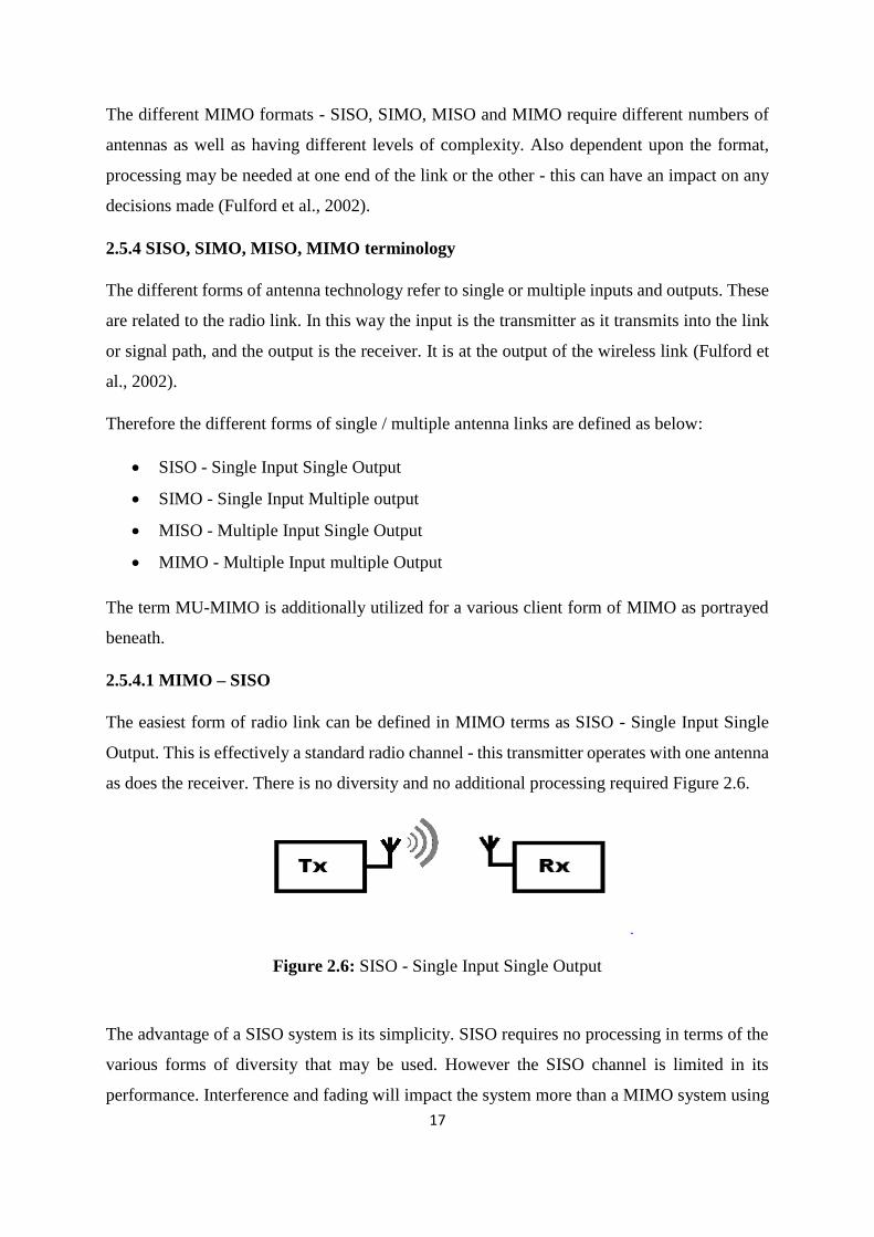
2.5.4.1 MIMO – SISO

The easiest form of radio link can be defined in MIMO terms as SISO - Single Input Single

Output. This is effectively a standard radio channel - this transmitter operates with one antenna

as does the receiver. There is no diversity and no additional processing required Figure 2.6.

Figure 2.6: SISO - Single Input Single Output

The advantage of a SISO system is its simplicity. SISO requires no processing in terms of the

various forms of diversity that may be used. However the SISO channel is limited in its

performance. Interference and fading will impact the system more than a MIMO system using

18

some form of diversity, and the channel bandwidth is limited by Shannon's law - the throughput

being dependent upon the channel bandwidth and the signal to noise ratio (Engels, 2002).

2.5.4.2 MIMO – SIMO

The SIMO or Single Input Multiple Output version of MIMO occurs where the transmitter has

a single antenna and the receiver has multiple antennas. This is also known as receive diversity.

It is often used to enable a receiver system that receives signals from a number of independent

sources to combat the effects of fading (Wood et al., 2008). It has been used for many years

with short wave listening / receiving stations to combat the effects of ionospheric fading and

interference Figure 2.7.

Figure 2.7: SIMO - Single Input Multiple Output

SIMO has the advantage that it is relatively easy to implement although it does have some

disadvantages in that the processing is required in the receiver. The use of SIMO may be quite

acceptable in many applications, but where the receiver is located in a mobile device such as a

cellphone handset, the levels of processing may be limited by size, cost and battery drain.

There are two forms of SIMO that can be used:

Switched diversity SIMO: This form of SIMO looks for the strongest signal and

switches to that antenna.

Maximum ratio combining SIMO: This form of SIMO takes both signals and sums

them to give the combination. In this way, the signals from both antennas contribute to

the overall signal.

19

2.5.4.3 MIMO – MISO

MISO is also called transmit diversity. In this case, the same data is transmitted excessively

from the two transmitter antennas. The receiver is then able to receive the optimum signal

which it can then use to receive extract the required data Figure 2.8.

Figure 2.8: MISO - Multiple Input Single Output

The advantage of using MISO is that the multiple antennas and the redundancy coding /

processing is moved from the receiver to the transmitter. In instances such as cellphone UEs,

this can be a significant advantage in terms of space for the antennas and reducing the level of

processing required in the receiver for the redundancy coding. This has a positive impact on

size, cost and battery life as the lower level of processing requires less battery consumption

(DVB, 2009).

2.5.4.4 MIMO

Where there is more than one antenna at either end of the radio link, this is termed MIMO -

Multiple Input Multiple Output. MIMO can be used to provide improvements in both channel

robustness as well as channel throughput Figure 2.9.

Figure 2.9: MIMO - Multiple Input Multiple Output

20

In order to be able to benefit from MIMO fully it is necessary to be able to utilize coding on

the channels to separate the data from the different paths. This requires processing, but

provides additional channel robustness / data throughput capacity.

There are many formats of MIMO that can be used from SISO, through SIMO and MISO to

the full MIMO systems. These are all able to provide significant improvements of performance,

but generally at the cost of additional processing and the number of antennas used. Balances of

performance against costs, size, processing available and the resulting battery life need to be

made when choosing the correct option (DVB, 2008)

21

CHAPTER 3

CLINICAL BACKGROUND

3.1 Medical Importance

Telemedicine is the application of advanced telecommunication technology for diagnostic,

monitoring and therapeutic purposes. It enables data transmission from the patient's

whereabouts or his/her primary care provider to a specialized medical call center (Reimers,

1996).

Telecardiology is one of the most highly developed of the medical disciplines covered by

telemedicine. In addition to the provision of care to patients with heart disease, it has a vital

role in educating these patients on the nature of their conditions, improving their compliance

to medical therapy, and guiding them in practicing healthy life habits. The benefit of

telecardiology in rural communities is especially important because of its capability of

overcoming the obstacle of the large distances that would have to be covered in order to access

medical assistance Figure 3.1

Figure 3.1: Telecardiology

22

Electrocardiogram (ECG or EKG) is a record of bio-electric potential variation recorded

through time on the body surface that represents heart beats [1]. Every heartbeat cycle is

normally characterized by the sequence of waveforms known as a P wave, QRS complex and

a T wave. Time intervals between those waveforms as well as their shapes and orientation are

representing physiological processes occurring in heart and autonomous nervous system.

Although today in medical centers advanced equipment and tools are used for detecting heart-

beat arrhythmias and other cardiovascular abnormalities, visual inspection of the multi-channel

(lead) ECG record is still the first step taken by cardiologists in diagnosis process (Ghaffari et

al., 2007) Figure.3.2.

Detailed explanation of the physiological process behind the ECG signal shape is out of the

scope of this thesis, but for the easier understanding of the main goals of this research a short

summary will be given.

Human heart is divided into four main chambers called atria and ventricles both with their left

and right instances. Those chambers together form a biological pump for propelling the blood

throughout the body. Besides those four obvious sections there are some other parts of the heart

for very specialized functions like dividing atria from ventricles, slow impulse propagation,

very fast impulse propagation etc., all of them performing particular tasks, ensuring that blood

flows properly and efficiently throughout the body. When electrical impulse propagates

Figure 3.2: Normal ECG signal with marked characters.

23

through heart and all these specialized cells, ECG electrodes pick up that impulse in various

directions and speed. In this way ECG waveforms are formed (Clifford et al., 2006) (Camm et

al., 2009). With that in mind one can logically assume that different problems in different kind

of cells or different parts of heart will have corresponding effects in ECG wave’s direction and

morphology (Luna, 2008).

Efficient and fast ECG analysis algorithms are needed in clinical practice but also in pre-

hospital use cases since clinical findings indicated that there was a significant improvement in

patient outcome based on this early treatment (Purvis et al., 1999). Pre-hospital ECG is a test

that may potentially influence the management of patients with acute myocardial infarction

through wider, faster in-hospital utilization of re-perfusion strategies and greater usage of

invasive procedures, factors that may possibly reduce short term mortality (Jakes, 1994).

Medical literature suggests clinical importance of ECG not only in identifying heart problems

itself, but also other health issues that leave a trace on ECG as a symptomatic phenomenon like

ECG patterns reflecting antidepressant treatment.

24

CHAPTER 4

DIGITAL VIDEO BROADCASTING

The Digital Video Broadcasting (DVB) specifications cover digital services delivered via

cable, satellite and terrestrial transmitters, as well as by the internet and mobile communication

systems. Digital Video Broadcasting (DVB) is playing a crucial role in digital television and

data broadcasting world-wide. DVB services have recently been introduced in Europe, in

North- and South America, in Asia, Africa and Australia. Among the more recent achievements

are the standards for terrestrial transmission, for microwave distribution and for interactive

services via PSTN/ISDN and via (coaxial) cable (Reimers, 1996). As it is stated by the standard

in (DVB, 2008) techniques used by DVB are able to deliver data at approximately 38 Mbit/s

within one satellite or cable channel or at 24 Mbit/s within one terrestrial channel. The satellite

member of the DVB family, DVB-S, is defined in European Standard EN 300 421 (ETSI,

1997)). September 1993, and at the end of the same year produced its first specification, DVB-

S (DVB, 2009), the satellite delivery specification now used by most satellite broadcasters

around the world for DTH (direct-to-home) television services. The DVB-S system is based on

QPSK modulation and convolutional forward error correction (FEC), concatenated with Reed-

Solomon coding. In 1998, DVB produced its second standard for satellite applications, DVB-

DSNG (DVB, 2010), extending the functionalities of DVB-S to include higher order

modulations (8PSK and 16QAM) for DSNG and other TV contribution applications by

satellite.

4.1 DVB Family

DVB contains a suite of standards for digital television. All of these standards are maintained

by DVB Project. DVB Project is formatted from a union of European broadcasters, equipment

manufacturers and other regulatory bodies in September 1993 and the purpose of this union

was to agree in which technology will be used in digital broadcasting. Currently DVB project

standards are used in more than 35 countries (mostly Europe) (DVB, 2009). DVB standard are

“divided” in three “traditional” standards which are DVB-S for satellite systems as in Figure

4.1, DVB-C for link systems and lastly DVB-T for terrestrial networks. Except for these main

standards, DVB project have some supporting standards which are needed to cover areas such

as service information (DVB-SI) and subtitles (DVB-SUB). In recent years, DVB added

standards for new technological areas such as handheld devices (DVB-H) and mobile TV

25

(DVB-SH) making the DVB family standards even bigger. At the end of 2009 DVB upgraded

two of first generation broadcasting standards to second generation standards (DVB-S2 and

DVB-T2). Currently DVB’s target is to upgrade the last of the first generation transmission

standards (DVB-H).

Figure 4.1: DVB-S system

4.1.1 DVB – T

DVB-T (Digital Video Broadcast – Terrestrial) is the most common used set of standards in

the world (mostly in Europe) for the terrestrial TV transmission. It was first published in late

1997 and now is used in more than 35 countries. DVB-T is designed to be compatible with

MPEG-2 coded TV signals (and lately MPEG-4 but not all of MPEG-4 standards) as well as

audio encoding systems and to work within the existing VHF and UHF The transmission is

based on Coded Orthogonal Frequency Division Multiplex (COFDM). COFDM uses a large

number of carriers. Each of these carriers is used to transmit only a portion of the total amount

of data. The data is modulated on the carriers with QPSK or QAM. COFDM has the advantage

that it is very robust against multipath reception and frequency selective fading. This robustness

against multipath reception is obtained through the use of a 'guard interval'. This is a proportion

of the time there is no data transmitted. This guard interval reduces the transmission capacity

(Shannon et al., 1990).

26

Because of this multipath immunity, it is possible to extend the coverage area with the use of

an overlapping network of transmitter stations which use the same frequency, a so-called

single frequency network (SFN). In the areas of overlap, the weaker of the two signals is

considered as an echo due to multipath reception. However, the stations have to be

synchronized and the echo has to fall within the guard time. Hence, if two stations are far apart,

the time delay between the two signals can be large and the system will need a large guard

interval (Chang, 1970).

There are two COFDM transmission modes possible in the DVB-T system. A 2k mode which

uses 1705 carriers and a 8k mode which uses 6817 carriers. The 2k mode is suitable for single

transmitter operation and for relatively small single frequency networks with limited

transmission power. The 8k mode can be used both for single transmitter operation and for

large area single frequency networks. The guard interval is selectable.

Portable and mobile reception of DVB-T signals is possible. It is even possible to mix the

reception modes by using hierarchical transmissions, in which one of the modulated streams

(so-called HP – High Priority stream), is given a higher protection against errors, to make is

suitable for mobile reception; while the other one (so-called LP – Low Priority stream), has a

lower protection. The higher protection mode will have a lower net bit rate available.

4.2 DVB – T coding and modulation

In the transmitter Figure 4.1, the first step is the encoding of image, audio and other data (if

those exist) and then multiplexing it with the MPEG-2 PS. One or more MPEG-PSs are joined

together into an MPEG transport stream (MPEG-TS).

The transfer rate starts from 5Mbit/sec and could rise to the 32Mbits/sec depending on

configuration and coding we choose in relation to the application we want to use.

Therefore, the selection of the video quality is the end users choice. First, the bit stream is

divided into sections of 188 bytes. To these we apply Reed-Solomon RS coding which provides

error correction up to 8 bytes (for each of these packages). These packages are then modulated

using QPSK (Quadrature Phase Shift Keying), 16QAM (Quadrature Amplitude Modulation)

27

or 64QAM While higher order modulation rates are able to offer much faster data rates and

higher levels of spectral efficiency for the radio communications system, this comes at a price.

The higher order modulation schemes are considerably less resilient to noise and interference

(DVB, 2009). QPSK is a phase modulation algorithm. It’s an improved algorithm based on

RSK configuration, using 4 possible states: 45, 135 225 and 315 degrees. QAM configuration

combines two signals into one channel. The final version of the QAM signal will have two

carriers on the same frequency that differ in phase by 90 degrees. After the modulation the

symbols are grouped in the blocks. Each of these blocks can have 1512, 3024 or 6048 symbols.

68 of these blocks are called one frame. After the blocks are formed by the algorithm OFDM

(Orthogonal Frequency Division Multiplexing) or COFDM (coded OFDM) guard intervals of

length 1/4, 1/8, 1/16 or 1/32 of total length of the block are imported. After that step the final

signal is modulated from digital to analog and transmitted in the air medium using a pre-set

bandwidth 6MHz, 7MHz or 8MHz. The reason we use the guard intervals is to avoid the ISI

(inter-symbol Interference) phenomenon that occurs when a signal reaches the receiver using

two different paths and resulting in weakening the signal. By importing the guard intervals in

our signal in a default time rate we succeed to synchronize our receiver with our signal. This

leads to a minor drawback, the small increase in the non-useful information we receive (DVB,

2008).

Figure 4.2: Block diagram of DVB-T system

28

4.3 Second Generation Digital Video Broadcasting over Satellite (DVB-S2)

Digital satellite transmission technology has evolved considerably since the publication of the

original DVB-S specification. New coding and modulation schemes permit greater flexibility

and more efficient use of capacity, and additional data formats can now be handled without

significant increase of system complexity. DVB-S2 Figure 4.3 has a range of constellations on

offer. DVB-S2 supports a wide range of modulation schemes, including QPSK (2bits/symbol),

8PSK (3bits/symbol), 16APSK (4bits/symbol) and 32APSK (5bits/symbol). These APSK

modulation schemes provide superior compensation for transponder non-linearity’s than QAM.

DVB-S2 is so flexible that it can cope with any existing satellite transponder characteristics,

with a large variety of spectrum efficiencies and associated SNR requirements. Furthermore it

is designed to handle a variety of advanced audio video formats which the DVB Project is

currently defining (DVB, 2008).

Figure 4.3: Block diagram of DVB-S2 system

Next, we will explain each block of Figure 4.3.

4.3.1 Data source

This the block represent the data of the ECG signal after being transformed into digital.

29

4.3.2 BCH encoder/decoder

One of DVB-S2 standard advances is the forward error correction which is deployed to reduce

BER in transmissions is BCH error correction. Output of BBFrame buffering block at the

sender side, as above mentioned, are frames of Kbch bits where a BCH (Nbch, Kbch) error

correction with the correcting power of t will be applied to them. For each of 11 rate of coding

presented in the standard Kbch and Nbch values are defined including the t-error correcting

parameter. In Table 4.1 these values are shown for normal and short frames respectively.

The output of BCH encoder called BCHFEC frame will be created by adding parity check bits

to make a frame with Nbch size. Nbch is the input of inner LDPC encoder which is also named

Kldpc.

4.3.3 LDPC encoder/decoder

Nbch, the BCH encoder output as the input of inner FEC encoder will be processed at LDPC

encoder to be protected from error with parity bits. The number of parity bits are given in

Tables 4.1 as:

Number of LDPC parity bits = Nldpc – Nbch.

LDPC encoder supports 11 coding rates. These coding rates are the ratio between information

bits (Nbch bits) and LDPC coded block bits which is the FECFRAME.

Table 4.1: Coding parameters for normal FECFRAME Nldpc=64800

LDPC

Code

BCH Uncoded

Block Kbch

BCH coded block Nbch

LDPC Uncoded Block k

Kldpc

BCH t-error

correction

LDPC Coded

Block

N

Nldpc

1/4 16008 16200 12 64800

1/3 21408 21600 12 64800

2/5 25728 25920 12 64800

½ 32208 32400 12 64800

3/5 38688 38880 12 64800

2/3 43040 43200 10 64800

3/4 484080 48600 12 64800

4/5 51648 51840 12 64800

5/6 53840 54000 12 64800

8/9 57472 57600 12 64800

9/10 58192 58320 12 64800

30

For example for rate 1/4 in a normal frame it means that for every 1 bit of information sent

from outer FEC coder (BCH), there will be 3 bits of parity checks added in LDPC encoder.

The lower this ratio the more protection of data against error has been carried out in LDPC

encoder. This will result in more robust data transmission, and it will reduce system throughput

indeed. At the receiver side, LDPC decoder will check the received sequence till the parity

checks are satisfied up to 50 iterations. This error correction uses the sparse parity-check

matrices with a hard decision making algorithm.

4.3.4 Block interleaving/deinterleaving

Interleaving process is the next step in DVB-S2 for modulations 8PSK, 16APSK and 32APSK.

Interleaving on QPSK is not going to be done and as for DVB-S2 model, 16APSK and 32APSK

modulations are not included so we will discuss them in our proposed model later.

Interleaver block in will make this an 8PSK by writing column wise serially the output of

LDPC encoder in a 3 by n ldpc (21600 for 8PSK) matrix and then will read it out row wise.

The MSB of BBHeader will be read-out first since for rate 3/5 it will be read-out as third.

Interleaving process creates rows in a matric from the LDPC encoder output according to the

modulation order M, so each row will contain a symbol ready to be mapped in the next block,

modulation. At the receiver side de-interleaver block will receive the output of demodulator

block as input and will apply the reverse process to create a serial output for the LDPC decoder

input.

4.3.5 QPSK modulation/demodulation

Modulation block will process the interleaved vector by first mapping each row to a symbol

which in our case is a gray mapping, then the mapped symbols will be assigned to

constellations.

4.3.6 Channel

The channel is the medium between the transmitter and receiver and it can be different types.

One of the most famous channel is the AWGN which represent the simple channel as the signal

suffer from only the additive white Gaussian noise (Reimers, 1990).

31

Another type is the MIMO channel which is represent multiple channel with different

condition.

32

CHAPTER 5

SIMULATION AND PERFORMANCE ANALYSIS

5.1 Introduction

In this chapter, two Telecardiology systems are assumed and simulations are run to see the

effects of transmitting ECG signals through these systems. Specifically, transmissions through

DVB-T and DVB-S2 systems are analyzed. MIMO is then added to the DVB-T system to see

how it changes the performance.

5.2 ECG signal generation

An ECG signal is obtained with the assistance of ECG electrodes. ECG sensors can be placed

at the midsection of the patient or generally at the wrist.

Figure 5.1: ECG system

This thesis does not use real ECG data. Therefore, first step in Telecardiology transmission

simulation becomes the ECG signal generation. In this section, we will show how computer

generated ECG signals for two different patients with different heart rates Figure 5.1 and Figure

5.2 can be transformed from analog into digital.

33

Figure 5.2: ECG signal of the first patient

Figure 5.3: ECG signal of the second patient

The procured ECG signals from the sensors are in analog form. These analog signals are sent

to the analog to digital converter (ADC) unit for conversion into computerized signal. In this

way, analog signals are changed over into digital signals. Conversion of analog signal into

digital includes the following three steps:

1. Sample the signal with high rates to capture all the changes in the ECG signal.

2. Quantize the sampled signal to approximate each sample to its proper level.

3. Encode the signal into binary data.

0 0.2 0.4 0.6 0.8 1 1.2 1.4 1.6 1.8 2-2

-1.5

-1

-0.5

0

0.5

1

1.5

2

Time [sec]

Volta

ge [m

V]

first patient Heartbeat Signal

0 0.2 0.4 0.6 0.8 1 1.2 1.4 1.6 1.8 2-2

-1.5

-1

-0.5

0

0.5

1

1.5

2

Time [sec]

Volta

ge [m

V]

Second patient Heartbeat Signal

34

Figure 5.4 shows the sampled ECG signal for the first patient and it is obtained by using

Simulink program. Sampling rate is taken to be 3 kHz as the input signal is not more than 200

Hz as the maximum heart rate for normal people when do running. According to Nyquist

equation the sampling frequency should be greater than double the input signal maximum

frequency. This allows us catch any variation on the signal like the unusual ECG signal for

people with heart problems.

Figure 5.4: Sampled representation of ECG signal

Second step in conversion is quantization. Figure 5.5 shows the ECG signal after being

quantized.

Figure 5.5: Quantized ECG signal

0 1 2 3 4 5 6

x 104

-1

-0.8

-0.6

-0.4

-0.2

0

0.2

0.4

0.6

0.8

1

number of samples

sign

al v

alue

0 1 2 3 4 5 6

x 104

-1

-0.8

-0.6

-0.4

-0.2

0

0.2

0.4

0.6

0.8

1

number of samples

signa

l valu

e

35

Figure 5.6 shows the difference (error) due to quantization between the two signals. Maximum

error is almost 0.032.

Figure 5.6: Error between quantized and sampled ECG signal

Figure 5.7 represents the ECG signal after being encoded into 8 bit codeword.

Figure 5.7: Binary representation of ECG Signal

5.3 Comparison of DVB-T with 64-QAM in AWGN Channel

One aim of this section is to analyze the performance of ECG transmission of Telecardiology

system using DVB-T technology with using 64-QAM modulation scheme in an additive white

Gaussian noise (AWGN) channel. The result is compared to theoretical bit error rate (BER) of

64-QAM, the modulation type chosen in DVB-T, in an AWGN channel. Figure 5.8 shows this

comparison.

BER Bit Error Rate Tutorial and Definition

0 1 2 3 4 5 6

x 104

-0.035

-0.03

-0.025

-0.02

-0.015

-0.01

-0.005

0

number of samples

signa

l valu

e

0 100 200 300 400 500 600 700 800 900 1000-1.5

-1

-0.5

0

0.5

1

1.5binary data of the quantized ecg signals

number of samples

signa

l valu

e

36

Bit error rate, BER is used to quantify a channel carrying data by counting the rate of errors

in a data string. It is used in telecommunications, networks and radio systems.

BER =𝑁𝑢𝑚𝑏𝑒𝑟 𝑜𝑓 𝑒𝑟𝑟𝑜𝑟𝑠

𝑇𝑜𝑡𝑎𝑙 𝑛𝑢𝑚𝑏𝑒𝑟 𝑜𝑓 𝑏𝑖𝑡𝑠

.

Figure 5.8: Comparison between DVB-T and theoretical 64-QAM in an AWGN channel

It can be seen from Figure 5.8 that DVB-T technology is 7 dB worse at 10-2 BER when

compared to the performance of theoretical 64-QAM.

5.4 Comparison between DVB-S2 and QPSK in AWGN Channel

In this section, a comparison is conducted between the performance of ECG transmission using

DVB-S2 technology with QPSK modulation scheme and theoretical BER of QPSK in an

AWGN channel see Figure 5.9. QPSK is the modulation type chosen in DVB-S2.

0 2 4 6 8 10 12 14 16 18 2010

-8

10-7

10-6

10-5

10-4

10-3

10-2

10-1

100

SNR [dB]

BE

R

DVB-T

64-QAM

37

Figure 5.9: Comparison between DVB-S2 and theoretical QPSK in an AWGN channel

Figure 5.9 shows that DVB-S2 technology is about 8.5 dB better than theoretical QPSK at a

BER of 10-5.

5.5 Comparison between DVB-T and DVB-S2 in AWGN Channel

One of the goals of this thesis is to see if a terrestrial or a satellite technology is more suitable

for Telecardiology. One way to check this is to observe the system performance during the

transmission of ECG signals using DVB-S2, a satellite technology, and DVB-T, a terrestrial

technology, in an AWGN channel. Figure 5.10 shows the performance comparison of ECG

transmission using DVB-S2 and DVB-T technologies in an AWGN channel.

It is shown that DVB-S2 performs much better than DVB-T in an AWGN channel. The

improvement is about 18-19 dB at 10-2 BER. The reasons for this most probably are the usages

of better error coding and modulation methods in DVB-S2.

0 2 4 6 8 10 12 14 16 18 2010

-8

10-7

10-6

10-5

10-4

10-3

10-2

10-1

100

SNR [dB]

BE

R

DVB-S2

QPSK

38

Figure 5.10: Performance of DVB-S2 and DVB-T in AWGN channel

5.6 Effect of MIMO on DVB-T Performance

In order to analyze how much of an improvement is obtained with the use of MIMO,

performance of transmission of ECG using DVB-T technology is compared to the performance

when MIMO is additionally included. This is shown in Figure 5.11, which clearly indicates an

about 5 dB gain of MIMO inclusion at 10-2 BER.

Figure 5.11: Effect of MIMO on DVB-T performance

0 2 4 6 8 10 12 14 16 18 2010

-5

10-4

10-3

10-2

10-1

100

SNR [dB]

BER

DVB-S2

DVB-T

0 2 4 6 8 10 12 14 16 18 2010

-6

10-5

10-4

10-3

10-2

10-1

100

SNR [dB]

BER

DVB-T

DVB-T with MIMO

39

CHAPTER 6

CONCLUSION

In this thesis we analyze if terrestrial or satellite transmission is better suited for ECG

transmission for remote heart monitoring in Telecardiology. It is hoped that using this

technology remote medical professionals such as doctors can accurately read and interpret the

ECG of a patient.

Specifically, DVB-T and DVB-S2 technologies are used for ECG transmission, after being

converted into digital. Simulations are carried out over Additive White Gaussian Channel

(AWGN) and bit error rate (BER) results are analyzed. Results are compared to theoretical

values as well. It is observed that for remote ECG transmission, performance improves by 18

dB if DVB-S2 technology is used over DVB-T technology.

It is known that wireless transmission suffers from multipath propagation. This is due to signals

reaching the receiver through different paths. One of the techniques for reducing the effects is

Multiple Input Multiple Output (MIMO) antenna technology. This thesis analyzes the

performance of ECG transmission through a multipath Rayleigh fading channel and shows that

with the addition of MIMO a performance gain of 5 dB is obtained.

Overall, DVB-S2 technology is shown to be superior to DVB-T for ECG transmission, both in

AWGN and in fading channels. However, it is known that satellite transmission suffers from

more delay and degradations than terrestrial transmission. Therefore, a trade-off exists such

that if performance loss can be tolerated then DVB-T technology might be used instead for

faster ECG transmission.

Future work will include analyzing other satellite, cable or terrestrial DVB standards for use

with ECG transmission as well as use of other techniques for mobile wireless systems, and also

applying equalization, and multipath fading reduction algorithms.

40

REFERENCES

(DVB), D. V. (1998). Frame structure channel coding and modulation for a 11/12 GHz

satellite services. European Telecommunications Standards Institute (ETSI). Retrieved

May 31, 1998 from

https://www.etsi.org/deliver/etsi_en/300400_300499/300421/01.01.02_60/en_300421

v010102p.pdf

(DVB), D. V. (2009). Frame structure channel coding and modulation for a second generation

digital terrestrial television broadcasting system (DVB-T2). European

Telecommunications Standards Institute (ETSI). Retrieved October 31, 2009 from

https://www.etsi.org/deliver/etsi_en/302700_302799/302755/01.03.01_40/en_302755

v010301o.pdf

(DVB), D. v. (2009). Framing structure, channel coding and modulation for 11/12 GHz

satellite services. European Telecommunications Standards Institute (ETSI). Retrieved

October 31, 2009 from

https://www.etsi.org/deliver/etsi_en/300700_300799/300744/01.06.01_60/en_300744

v010601p.pdf

(DVB), D. v. (2010). Framing structure, channel coding and modulation for DSNG and other

contribution applications by satellite. European Telecommunications Standards

Institute(ETSI). Retrieved May 31, 2010 from

https://www.etsi.org/deliver/etsi_en/302300_302399/302307/01.02.01_60/en_302307

v010201p.pdf

(DVB), D. v. (2013). Implementation guidelines for the use of MPEG-2 systems, video and

audio in satellite, cable and terrestrial broadcasting applications. European

Telecommunications Standards Institute (ETSI). Retrieved December 31, 2013 from

https://www.etsi.org/deliver/etsi_en/302300_302399/302307/01.03.01_60/en_302307

v010301p.pdf

(DVB), D. v. (2010). Second generation framing structure, channel coding and modulation

systems for broadcasting, interactive services, news gathering and other broad-band

41

satellite applications. European Telecommunications Standards Institute (ETSI).

Retrieved May 31, 2010 from

https://www.etsi.org/deliver/etsi_en/302300_302399/302307/01.02.01_60/en_302307

v010201p.pdf

(2010). Frame structure channel coding and modulation for a second generation digital

terrestrial television broadcasting system (DVB-T2). Digital Video Broadcasting.

Retrieved June 30, 2010 from

https://www.etsi.org/deliver/etsi_en/302700_302799/302755/01.01.01_60/en_302755

v010101p.pdf

Shannon, C.E. (1948). A Mathematical Theory of Communication. Bell System Technical

Journal, ( 8, 397–423).

Camm, A., L¨uscher, T., & Serruys, P. (2009). The ESC Textbook of Cardiovascular Medicine.

OUP Oxford.

Chang, R. W. (1970). Patent 3,488,455. U.S.

Clifford, G. D., Azuaje, F., & McSharry, P. (2006). Advanced Methods And Tools for ECG

DatabAnalysis. MA, USA: Artech House, Inc.

Engels, M. (2002). Wireless OFDM Systems: How to make them work? Kluwer Academic.

Fulford-Jones, T. R., Wei, G., & Welsh, M. (2004). Aportable low-power, wireless two-lead

EKG System. IEEE Engineering in Medicine and Biology Society (pp. 2141-2144). San

Francisco: Calif USA.

Ghaffari, A., Golbayani, H., & Ghasemi, M. (2007). A new mathematical based qrs detector

using continuous wavelet transform. Computer Electical. Engineering, 81-91.

Jakes, W. (1994). Microwave Mobile Communications. Piscataway, NJ: IEEE Press.

Luna, A. d. (2008). Basic Electrocardiography: Normal and Abnormal ECG Patterns. John

Wiley & Sons.

42

Reimers, U. (1996). A Guideline for the Use of DVB Specifications and Standards. DVB

Document TM 1694.

Sklar, B. (1997). Rayleigh Fadin Channels in mobile Digital Communications part I:

Characterization. IEEE Communication Magazine, 90-100.

Ubeyli, E. D. (2008). Implementing wavelet transform/mixture of experts network for analysis

of electrocardiogram beats. Expert Systems, (Vol. 25, pp. 150-162).

Wood, A. D., Stankovic, J. A. & Virone, G. (2008). Context-aware wireless sensor networks

for assisted living and residential monitoring. IEEE Network, 26-33.

43

APPENDIX

SOURCE CODE

Source codes for the simulation models used in this thesis are given below:

A.1. Create heart beat data

This code is used to generate the heart beat data.

%%%%%%%%%%%%%%%%%%%%%%%%%%%%%%%%%%%%%%%%%%%%%

%%%%%%%%%%%%%

clc

clear all

close all

x1 = 1*ecg(8000).';

y1 = sgolayfilt(kron(ones(1,26),x1),0,21);

n = 1:63168;

del = round(50*rand(1));

mhb = y1(n + del);

t = 0:3.1662e-5:2;

data.time=t';

data.signals.values =mhb;

data.signals.dimensions =1;

save('ecg','data');

save('hany','t','mhb')

plot(t,mhb);

axis([0 2.5 -2 2]);

grid;

xlabel('Time [sec]');

ylabel('Voltage [mV]');

title('Maternal Heartbeat Signal');

44

A.2. Create digital data for Simulink

This MATLAB code is used to convert the ECG signal from analog into digital.

%%%%%%%%%%%%%%%%%%%%%%%%%%%%%%%%%%%%%%%%%%%%%

%%%%%%%%%%%%%%

clc

clear all

close all

load heart_beat

x=mhb;%the samples

N=10;% no of bit for each sample

R=2^N;% the no of qunatized level

a=linspace(-1,1,R); % rangens for N bit

b=0:R-1;

y=quantiz(x,a,b);

xq=(y/max(y)-.5)*2;

e=x-(xq);

y1=de2bi(y);

y2=reshape(y1',1,numel(y1));

S1=1504;

T1=211;

y3=y2(1:S1*T1);

y4=reshape(y3,S1,T1);

N1=zeros(S1,1,T1);

for ii=1:T1

N1(:,:,ii)=y4(:,ii);

end

sample=logical(N1);

step=0.0476;

45

tout=0:step:10;

y3=timeseries(sample,0:step:10);

% save the varaiable for the simulink

save('w_ecg','tout','sample')

save('w_ecg1','y3')

plot(x,'b')

title('the ecg signal')

xlabel('the samples')

ylabel('signal value')

grid on

figure

plot(xq,'b')

title('the quantized ecg signal')

xlabel('the samples')

ylabel('signal value')

grid on

figure

plot(e,'r')

grid on

title('the error between quantized and ecg signals')

xlabel('the samples')

ylabel('signal value')

xlabel('the samples')

ylabel('signal value')

figure

stem(y2(1:1000))

grid on

title('binary data of the quantized ecg signals')

xlabel('the samples')

ylabel('signal value')

46

axis([0 1000 -1.5 1.5])

A.3.Create comparison figures

This MATLAB code creates the comparison figures

%%%%%%%%%%%%%%%%%%%%%%%%%%%%%%%%%%%%%%%%%%%%%

%%%%%%%%%%%%

clc

clear all

close all

%%%%%% the DVB S2 with our ECG data

load('default qpsk_64qam.mat')

snr=0.1:0.1:1;

ber_s2=[0.1238 0.1176 0.1107 0.1028 0.09281 0.08156 0.05252

0.006651 0.0003 0.00002];

ber_s2_m=1e-7*ones(1,10);

ebn0=0:20;

snr1=[snr 2 3 4 5 6 7 8 9 10 12 14 16 18 20];

ber_t_m=[0.493 0.4916 0.4909 0.4901 0.4893 0.4886 0.4877 0.486

0.485 0.482 0.471 0.444 0.396 0.3 0.2061 0.1176 0.05362 0.0174

0.0075 0.002 0.0004 0.00007 0.00001 0.000001];

ber_t_m1=[0.493 0.4893 0.4886 0.4877 0.486 0.485 0.482 0.471

0.444 0.396 0.3 0.2061 0.1176 0.05362 0.0174 0.0075 0.002

0.0004 0.00007 0.00001 0.000001];

ber_t=[0.499 0.499 0.499 0.499 0.499 0.499 0.499 0.499 0.499

0.499 0.449 0.498 0.498 0.498 0.498 0.498 0.497 0.497 0.497

0.44 0.3205 0.090 0.048 0.005];

ber_t1=[0.499 0.499 0.499 0.499 0.499 0.499 0.499 0.449 0.498

0.498 0.498 0.498 0.498 0.497 0.497 0.497 0.44 0.3205 0.090

0.048 0.005];

snr2=[0 1 2:20];

%%%%%%%%%%%%%%%%%

figure

semilogy(snr2,ber_t1,'k*-')

hold on

semilogy(ebn0,ber_qam,'ro-')

47

grid on

xlabel('SNR')

ylabel('BER')

legend('the DVB-T ','64-QAM')

%%%%%%%%%%%%%%%%%%%%%%%%%%%%%%%%%%%

figure

semilogy(snr,ber_s2,'k*-')

hold on

semilogy(ebn0,ber_qpsk,'ro-')

grid on

xlabel('SNR')

ylabel('BER')

legend('DVB-S2 ','QPSK')

axis([0 20 1e-8 1])

%%%%%%%%%%%%%%%%%%%%%%%%%%%%%%%

figure

semilogy(snr2,ber_t_m1,'r*-')

grid on

xlabel('SNR')

ylabel('BER')

%title('the DVB t-mimo result')

legend('DVB-T with MIMO')

%%%%%%%%%%%%%%%%%%%%%%%%%%%%%%%

figure

semilogy(snr,ber_s2,'k*-')

hold on

semilogy(snr2,ber_t1,'ro-')

48

grid on

xlabel('SNR')

ylabel('BER')

%title('the DVB comparisson result')

legend('DVB-S2 ','DVB-T')

%%%%%%%%%%%%%%%%%%%%%%%%%%%%%%

figure

semilogy(snr2,ber_t1,'k*-')

hold on

semilogy(snr2,ber_t_m1,'ro-')

grid on

xlabel('SNR')

ylabel('BER')

%title('the DVB t result')

legend('DVB-T ','DVB-T with MIMO')

%%%%%%%%%%%%%%%%%%%%%%%%%%

figure

semilogy(snr,ber_s2,'k*-')

hold on

semilogy(snr2,ber_t_m1,'ro-')

grid on

xlabel('SNR')

ylabel('BER')

%title('the DVB t result')

legend('DVB-S2 ','DVB-T with MIMO')

49

%%%%%%%%%%%%%%%%%%%%%%%%%%%%%%%%%%%%%%%%%%%%%

%%%%%%%%%%%%%%%%%%%

A.4. Simulink model for DVB-T with AWGN

A.5. Simulink model for DVB-T with MIMO:

50

A.6. Simulink model for DVB-S2 with AWGN

51