Technical Report Documentation Page

1. Report No.

FHWA/TX-13/0-6255-1

2. Government Accession No.

3. Recipient’s Catalog No.

4. Title and Subtitle

Use of Manufactured Sands for Concrete Pavement

5. Report Date

October 2012; Published August 2013

6. Performing Organization Code 7. Author(s)

David Whitney, Dr. David W. Fowler, Marc Rached

8. Performing Organization Report No.

0-6255-1

9. Performing Organization Name and Address

Center for Transportation Research The University of Texas at Austin 1616 Guadalupe St, Suite 4.202 Austin, TX 78701

10. Work Unit No. (TRAIS) 11. Contract or Grant No.

0-6255

12. Sponsoring Agency Name and Address

Texas Department of Transportation Research and Technology Implementation Office P.O. Box 5080 Austin, TX 78763-5080

13. Type of Report and Period Covered

Technical Report September 2008–August 2012

14. Sponsoring Agency Code

15. Supplementary Notes Project performed in cooperation with the Texas Department of Transportation and the Federal Highway Administration.

16. Abstract Manufactured fine aggregates are a product created when rocks are crushed using a mechanical crusher.

With the depletion of sources of natural sands, the usage of manufactured fine aggregates has increased. Manufactured fine aggregates have properties that differ from natural sands; for this reason, the plastic and hardened properties of concrete produced using manufactured fine aggregates differ from the properties of concrete made with natural sands. The main concrete properties affected by the usage of manufactured fine aggregates are skid resistance, workability, and finishability. The aim of this research project was to investigate how manufactured fine aggregates could be used in concrete pavements without causing workability or skid related issues. To improve the workability of concrete made with manufactured fine aggregates, the use of the optimized mixture proportioning method developed by the International Center for Aggregate Research (ICAR) was investigated. Results obtained from this testing were used to make recommendations on how to optimize class P concrete mixtures made with any type and combination of aggregates. 17. Key Words

Manufactured, sands, concrete pavement

18. Distribution Statement

No restrictions. This document is available to the public through the National Technical Information Service, Springfield, Virginia 22161; www.ntis.gov.

19. Security Classif. (of report) Unclassified

20. Security Classif. (of this page) Unclassified

21. No. of pages 204

22. Price

Form DOT F 1700.7 (8-72) Reproduction of completed page authorized

Use of Manufactured Sands for Concrete Pavement David Whitney Dr. David W. Fowler Marc Rached CTR Technical Report: 0-6255-1 Report Date: October 2012; Published August 2013 Project: 0-6255 Project Title: Use of Manufactured Sands for Concrete Paving Sponsoring Agency: Texas Department of Transportation Performing Agency: Center for Transportation Research at The University of Texas at Austin Project performed in cooperation with the Texas Department of Transportation and the Federal Highway Administration.

Center for Transportation Research The University of Texas at Austin 1616 Guadalupe St, Suite 4.202 Austin, TX 78701 www.utexas.edu/research/ctr Copyright (c) 2013 Center for Transportation Research The University of Texas at Austin All rights reserved Printed in the United States of America

v

Disclaimers Author's Disclaimer: The contents of this report reflect the views of the authors, who

are responsible for the facts and the accuracy of the data presented herein. The contents do not necessarily reflect the official view or policies of the Federal Highway Administration or the Texas Department of Transportation (TxDOT). This report does not constitute a standard, specification, or regulation.

Patent Disclaimer: There was no invention or discovery conceived or first actually reduced to practice in the course of or under this contract, including any art, method, process, machine manufacture, design or composition of matter, or any new useful improvement thereof, or any variety of plant, which is or may be patentable under the patent laws of the United States of America or any foreign country.

Notice: The United States Government and the State of Texas do not endorse products or manufacturers. If trade or manufacturers' names appear herein, it is solely because they are considered essential to the object of this report.

Engineering Disclaimer NOT INTENDED FOR CONSTRUCTION, BIDDING, OR PERMIT PURPOSES.

Project Engineer: Dr. David W. Fowler

Professional Engineer License State and Number: Texas No. 27859 P. E. Designation: Research Supervisor

vi

Acknowledgments The researchers had considerable assistance from many sources. Without their help, this

research could not have been completed. From TxDOT, the help of Ryan Barborak, Lisa Lukafahr, Dr. German Claros, Caroline Herrera, William Pecht, and Ed Morgan is gratefully acknowledged. In addition, the assistance of several TxDOT Districts proved to be essential during the course of the project.

The assistance of several people from the International Grooving and Grinding Association was essential to the conduct of the grooving and grinding portion of the research. In particular, John Robert, Gary Aamold, and Dan Frentress were very cooperative and helpful.

Lucas Steiner and Garth Taylor of Metso Minerals Test Center provided able assistance in the study of crusher speeds on the performance of manufactured sands. The laboratory research could not have been performed without the loan of the laboratory scale grinder.

There were many people at the Construction Materials Research Lab who must be acknowledged: staff technician Michael Rung; graduate students Michael De Moya, Chris Clement, and Sarwar Siddiqui; and undergraduate assistants Karla Kruse, Efren Tavira, Claudia Patterson, Pilar Guerrero, Nicole Rockey, and Joseph Fraccaro. Their help in making concrete specimens, setting up and repairing equipment, performing tests, taking field readings, and generally providing moral support is greatly appreciated.

vii

Table of Contents

Introduction.................................................................................................................1 Chapter 1. Introduction ............................................................................................................................1 1.1 Background ............................................................................................................................2 1.2 Problem Statement .................................................................................................................2 1.3 Research Objectives ...............................................................................................................3 1.4

Aggregates in Concrete Literature Review ..............................................................5 Chapter 2. Aggregate Properties ..............................................................................................................5 2.1

Shape ...............................................................................................................................5 2.1.1 Texture ............................................................................................................................7 2.1.1 Grading ...........................................................................................................................7 2.1.2 Absorption .......................................................................................................................9 2.1.3 Mineralogy ......................................................................................................................9 2.1.4

Durability of Fine Aggregates for Paving Concrete ............................................................11 2.2 Acid Insoluble Residue Test .........................................................................................11 2.2.1 Magnesium Sulfate Test................................................................................................11 2.2.2 Micro-Deval ..................................................................................................................12 2.2.3

Production of Manufactured Sands ......................................................................................12 2.3 Blended Sands in Concrete Pavements ................................................................................13 2.4 Approaches for Optimizing Aggregate Gradation ...............................................................14 2.5

Packing Density Method ...............................................................................................14 2.5.1 Surface Area ..................................................................................................................14 2.5.2 0.45 Power Chart ..........................................................................................................14 2.5.3 Coarseness Factor Chart................................................................................................15 2.5.4 Percent Retained ...........................................................................................................17 2.5.5

Concrete Properties and Performance Literature Review ...................................19 Chapter 3. Effect of Fine Aggregates on Fresh Concrete Properties ....................................................19 3.1

Workability ...................................................................................................................19 3.1.1 Finishability ..................................................................................................................20 3.1.2 Bleeding and Segregation .............................................................................................20 3.1.3 Air Content ....................................................................................................................20 3.1.4

The Effect of Fine Aggregates on Hardened Concrete Properties .......................................20 3.2 Strength .........................................................................................................................21 3.2.1 Shrinkage ......................................................................................................................21 3.2.2 Skid Resistance .............................................................................................................21 3.2.3

Evaluating Pavement Skid Performance ..............................................................................28 3.3 Test Methods for Evaluating Texture ...........................................................................28 3.3.1 Test Methods for Evaluating Friction ...........................................................................29 3.3.2 Accelerated Wear and Polishing Devices .....................................................................30 3.3.3 Correlating Skid Values Measured by Different Devices .............................................30 3.3.4

Diamond Grinding and Grooving ........................................................................................32 3.4 Mix Proportioning Methods for Portland Cement Concrete ...............................................33 3.5

ACI Mixture Design Method ........................................................................................33 3.5.1

viii

ICAR Method for Proportioning Concrete ...................................................................33 3.5.2

Material Properties ...................................................................................................37 Chapter 4. Cementitious Material and Admixtures ...............................................................................37 4.1 Fine Aggregates ...................................................................................................................37 4.2

Sieve Analysis ...............................................................................................................39 4.2.1 Dry-rodded Unit Weight and Uncompacted Void Test ................................................39 4.2.2 Methylene Blue Test .....................................................................................................40 4.2.3 Specific Gravity, Absorption, Acid Insoluble Residue, and Micro-Deval ...................40 4.2.4

Coarse Aggregates ...............................................................................................................43 4.3 Conclusions ..........................................................................................................................44 4.4

Non-Standard Micro-Deval Aggregate Testing .....................................................45 Chapter 5. Testing Fine Aggregates Using the Micro-Deval Apparatus ...............................................45 5.1 Testing Mortar Abrasion Using the Micro-Deval Apparatus ..............................................49 5.2 Conclusions ..........................................................................................................................56 5.3

Evaluating the Shape of MFA .................................................................................57 Chapter 6. Introduction ..........................................................................................................................57 6.1 Uncompacted Void Test Results ..........................................................................................59 6.2 AIMS Results .......................................................................................................................60 6.3 Mortar Flow Test .................................................................................................................62 6.4 Conclusions ..........................................................................................................................66 6.5

Proportioning PCC Containing MFAs ...................................................................67 Chapter 7. The ICAR Proportioning Method ........................................................................................67 7.1 Preliminary Modifications to the ICAR Proportioning Method ..........................................68 7.2 Evaluating the ICAR Method ..............................................................................................71 7.3 Determining the Optimum Paste Content for Pavement Concrete ......................................76 7.4 Recommendations ................................................................................................................77 7.5 Conclusions ..........................................................................................................................78 7.6

Preliminary Skid Testing .........................................................................................81 Chapter 8. Evaluating the Texture of Concrete Made by Different Finishing Techniques ...................82 8.1 Establishing a Testing Protocol for Testing Texture and Friction at the Laboratory ..........86 8.2 Conclusions ..........................................................................................................................92 8.3

Field Testing for Skid Resistance ............................................................................93 Chapter 9. Test Equipment Correlation .................................................................................................93 9.1 Sections Made with 100% MFA ..........................................................................................95 9.2

Construction of the 100% MFA Sections .....................................................................95 9.2.1 Texture and Friction Evaluation of 100% MFA Sections...........................................100 9.2.2

Blended Sand Sections .......................................................................................................102 9.3 Analysis and Conclusions ..................................................................................................104 9.4

Evaluation of Hardened Concrete Properties ....................................................107 Chapter 10. Mixing and Testing Procedures .......................................................................................107 10.1 Evaluating the Effect of Fine Aggregates on Hardened Concrete Properties ..................109 10.2

Mixture Proportions ..................................................................................................109 10.2.1 Siliceous Sands vs. Manufactured Sands ..................................................................109 10.2.2

ix

Blended Sands ..................................................................................................................118 10.3 Conclusions ......................................................................................................................127 10.4

Evaluating the Effect of Mixture Proportions on Texture and Friction Chapter 11.of PCC .........................................................................................................................................129

Mixture Proportions .........................................................................................................129 11.1 Effects of Varying Mixture Proportions on Limestone Sands .........................................129 11.2 Effects of Varying Mixture Proportions on Friction Resistance on Any Type of 11.3

Sand .........................................................................................................................................132 Effects of Adding Water onto the Concrete Surface .......................................................135 11.4 Conclusions ......................................................................................................................136 11.5

Evaluating Diamond Grinding and Grooving for Friction ..............................137 Chapter 12. Introduction ......................................................................................................................137 12.1 Results ..............................................................................................................................139 12.2 Conclusions ......................................................................................................................140 12.3

Analysis of Skid Data, Blending Recommendations, and Development Chapter 13.of a Skid Prediction Model for Concrete Pavements ..............................................................141

Alternative Method for Identifying Polish Resistant Sands ............................................141 13.1 Analysis of Data ........................................................................................................141 13.1.1 Recommendations .....................................................................................................145 13.1.2

Developing a Prediction Model .......................................................................................147 13.2 Introduction ...............................................................................................................147 13.2.1 Field Data Analysis ...................................................................................................147 13.2.2 Effect of Mixture Variables on Surface Friction ......................................................149 13.2.3 Relationship between DFT and MD .........................................................................150 13.2.4 Relationship between DFT and AI ...........................................................................151 13.2.5 Prediction Model for Computing SN(50)smooth .........................................................151 13.2.6 Verification of Prediction Model and Development of Design Charts .....................154 13.2.7

Conclusions ......................................................................................................................157 13.3

Summary and Conclusions ..................................................................................159 Chapter 14. Summary ..........................................................................................................................159 14.1

Finding a Fine Aggregate Test that Predicts Skid Performance ...............................159 14.1.1 Evaluating the Shape of MFA Produced Using Different Crushing Operations ......159 14.1.2 Proportioning Method for Pavement Concrete Containing MFA .............................160 14.1.3 Developing a Laboratory Skid Test ..........................................................................160 14.1.4 Evaluating the Skid Resistance of Pavements Made with Sands that Do Not 14.1.5

Meet Specifications ..............................................................................................................160 Laboratory Concrete Tests ........................................................................................161 14.1.6 Correlating Aggregate Tests to Laboratory Concrete Tests ......................................161 14.1.7 Recommendations and Prediction Formula ..............................................................161 14.1.8

Conclusions ......................................................................................................................161 14.2 Significance of Findings ..................................................................................................162 14.3

References ...................................................................................................................................163

Appendix A: Skid Testing Results ............................................................................................171

x

Appendix B: Texture and Friction Test Results .....................................................................179

Appendix C: Diamond Grinding and Grooving Test Results ................................................183

xi

List of Figures

Figure 2.1: Particle Shape ............................................................................................................... 6

Figure 2.2: Modified 0.45 Power Chart [Koehler and Fowler 2007] ........................................... 15

Figure 2.3: Coarseness Chart Proposed by Shilstone ................................................................... 16

Figure 2.4: “18-8” Percent Retained Chart ................................................................................... 17

Figure 3.1: Friction Force ............................................................................................................. 22

Figure 3.2: Hydroplaning .............................................................................................................. 22

Figure 3.3: Schematic Plot of Adhesion and Hysteresis [adapted from Hall et al., 2006] ........... 23

Figure 3.4: Pavement Wavelength and Surface Characteristics [adapted from Hall et al., 2006; Hoerner, 2003] ........................................................................................................ 24

Figure 3.5: Type of Texture Contributing to Texture ................................................................... 24

Figure 3.6: Effect of Siliceous Particle Content on Wear Index [Balmer and Colley, 1966] ....... 27

Figure 3.7: Correlation between SN(64)ribbed and DFT60 (metric units) [Heitzman, 2011] ......... 32

Figure 3.8: Factors Affecting Diamond-Ground Surfaces ............................................................ 32

Figure 3.9: Modified 0.45 Power Curve (Fowler and Koehler 2007) .......................................... 34

Figure 3.10: Paste Needed to Fill Voids between Aggregates [Koehler and Fowler, 2007] ........ 35

Figure 5.1: Micro-Deval Jar .......................................................................................................... 45

Figure 5.2: Varying Run Time for Micro-Deval Fine Aggregate Testing .................................... 46

Figure 5.3: Hanson Servtex Before and After Micro-Deval (120 Minutes Run time) ................. 46

Figure 5.4: Fine and Coarse Aggregate Sizes Compared to 10mm Ball Bearings ....................... 47

Figure 5.5: Percent Change in Gradation After 15 Minutes in the Micro-Deval Test .................. 48

Figure 5.6: Percent Change in Gradation After 60 Minutes in the Micro-Deval Test .................. 48

Figure 5.7: Percent Change in Gradation After 120 Minutes in the Micro-Deval Test ................ 49

Figure 5.8: 9 Abrasion of Mortar Specimens Using 3000g of Ball Bearings ............................... 51

Figure 5.9: 7 Abrasion of Mortar Specimen Using 1200g of Ball Bearings ................................ 51

Figure 5.10: Mortar Brownies Made with Siliceous Sand at a Water-to-cement Ratio of 0.45 and 0.6 ....................................................................................................................... 51

Figure 5.11: Mortar Specimen Tested Using Original AIMS Apparatus ..................................... 52

Figure 5.12: AIMS Texture Index Results Using the Original AIMS Device.............................. 52

Figure 5.13: New AIMS Apparatus (AIMS 2.0) .......................................................................... 53

Figure 5.14: AIMS Texture Index Results Using the New AIMS Device ................................... 54

xii

Figure 5.15: Mortar Specimen Tested for Texture (from left to right: Lattimore Stringtown, Colorado River Sand, and Texas Crushed Stone) ......................................... 54

Figure 5.16: Abraded Lattimore Stringtown and Colorado River Sand Mortar Specimens ......... 55

Figure 5.17: AIMS Color Test ...................................................................................................... 55

Figure 5.18: Larger Mortar Specimen For Testing Polish Resistance .......................................... 56

Figure 6.1: Aggregates Retained on the No. 8 sieve (from left to right: Colorado River Sand, Hanson Perch Hill, and Lattimore Stringtown) ...................................................... 58

Figure 6.2: Aggregates Retained on the No. 8 sieve (from left to right: Colorado River Sand, Hanson Perch Hill (Metso 60 m/s), and Hanson Perch Hill) .................................. 58

Figure 6.3: Aggregates Retained on the No. 8 sieve (from left to right: Colorado River Sand, Lattimore Stringtown (Metso 65 m/s), and Lattimore Stringtown) ........................ 58

Figure 6.4: Uncompacted Void Test for the Hanson Perch Hill Aggregates ................................ 59

Figure 6.5: Uncompacted Void Test for the Lattimore Stringtown Aggregates ........................... 59

Figure 6.6: Cumulative 2D Form Index for the Hanson Perch Hill Aggregate ............................ 60

Figure 6.7: Cumulative 2D Form Index for the Lattimore Stringtown Aggregate ....................... 61

Figure 6.8: Cumulative Angularity Index for the Hanson Perch Hill Aggregate ......................... 61

Figure 6.9: Cumulative Angularity Index for the Lattimore Stringtown Aggregate .................... 62

Figure 6.10: Mortar Flow Test Results for Hanson Perch Hill (grading as obtained from source) ............................................................................................................................... 63

Figure 6.11: Mortar Flow Test Results for Lattimore Stringtown (grading as obtained from source) ...................................................................................................................... 64

Figure 6.12: Mortar Flow Test Results for Hanson Perch Hill (graded sand) .............................. 65

Figure 6.13: Mortar Flow Test Results for Lattimore Stringtown (graded sand) ......................... 65

Figure 7.1: Visual Shape and Angularity Rating Scale McLeroy (2009) ..................................... 68

Figure 7.2: Flow of Aggregates with Different Shape and Angularity (5.5 sacks) ...................... 70

Figure 7.3: Flow of Aggregates with Different Shape and Angularity (6 sacks) ......................... 70

Figure 7.4: Capital Marble Falls S/A=0.30 (Modified 0.45 Power Chart) ................................... 71

Figure 7.5: Capital Marble Falls S/A=0.37 (Conventional 0.45 Power Chart) ............................ 72

Figure 7.6: Colorado River Sand S/A=0.30 (Modified 0.45 Power Chart) .................................. 72

Figure 7.7: Colorado River Sand S/A=0.37 (Conventional 0.45 Power Chart) ........................... 73

Figure 7.8: Texas Crushed Stone S/A=0.30 (Modified 0.45 Power Chart) .................................. 73

Figure 7.9: Hanson Servtex S/A=0.30 (Modified 0.45 Power Chart) .......................................... 74

Figure 7.10: Example of a 0.45 Power Chart ................................................................................ 78

Figure 7.11: Example of a Combined DRUW Test ...................................................................... 78

xiii

Figure 8.1: Circular Track Meter .................................................................................................. 81

Figure 8.2: Dynamic Friction Tester ............................................................................................. 81

Figure 8.3: Broom Finish .............................................................................................................. 82

Figure 8.4: Burlap Drag ................................................................................................................ 82

Figure 8.5: Tined + Burlap Drag .................................................................................................. 82

Figure 8.6: Trowel Finish ............................................................................................................. 82

Figure 8.7: Painted Glass .............................................................................................................. 83

Figure 8.8: Texture Profiles .......................................................................................................... 83

Figure 8.9: Measured MPD Range for the Different Textures ..................................................... 84

Figure 8.10: DFT Values for the Different Textures .................................................................... 84

Figure 8.11: DFT20 Values for Different Textures ...................................................................... 85

Figure 8.12: DFT60 Values for Different Textures ...................................................................... 85

Figure 8.13: NCAT Three-Wheel Polishing Device ..................................................................... 86

Figure 8.14: Wheels Used on the Polisher .................................................................................... 87

Figure 8.15: Pneumatic Wheels .................................................................................................... 87

Figure 8.16: Polyurethane Wheels ................................................................................................ 88

Figure 8.17: Steel Wheels ............................................................................................................. 89

Figure 8.18: Change in Texture Values for the River Sand and Limestone MFA ....................... 90

Figure 8.19: Change in Friction Values for the River Sand and Limestone MFA ....................... 90

Figure 8.20: Slab Made with Siliceous Sand ................................................................................ 91

Figure 8.21: Slab Made with Limestone MFA ............................................................................. 91

Figure 8.22: Surface Made with Siliceous Sand vs. Limestone MFA .......................................... 92

Figure 9.1: Computed vs. Measured SN(50)smooth ........................................................................ 93

Figure 9.2: DFT20 vs. Measured SN(50)smooth ............................................................................. 94

Figure 9.3: DFT60 vs. Measured SN(50)smooth ............................................................................. 94

Figure 9.4: MPD vs. Measured SN(50)smooth ................................................................................ 95

Figure 9.5: Low Slump Concrete - 5% Microfine Mixture [McLeroy, 2008] .............................. 98

Figure 9.6: Concrete with a Slump Exceeding the Requirements [McLeroy, 2008] .................... 98

Figure 9.7: Finishability Problems Encountered with 100% MFA Sections [McLeroy, 2008] ................................................................................................................................. 99

Figure 9.8: 100% MFA Sections December 2010 ...................................................................... 100

Figure 9.9: Computed Skid Numbers for Trial Field Sections as a Function of Time ............... 101

Figure 9.10: Section 1 Wheel Path (left) vs. Between Wheel Path (right) ................................. 101

xiv

Figure 9.11: Section 2 Wheel Path (left) vs. Between Wheel Path (right) ................................. 102

Figure 9.12: Section 3 Wheel Path (left) vs. Between Wheel Path (right) ................................. 102

Figure 9.13: Section 4 Wheel Path (left) vs. Between Wheel Path (right) ................................. 102

Figure 9.14: 60/40 Blended Section Wheel Path (left) vs. Between Wheel Path (right) ............ 103

Figure 9.15: SN(50)smooth for Blended Sand Sections Computed Using DFT60 ........................ 104

Figure 9.16: MPD vs. Measured SN(50)smooth ............................................................................ 105

Figure 10.1: Typical Markings on a Slab.................................................................................... 108

Figure 10.2: Modified Three-Wheel Polishing Device ............................................................... 108

Figure 10.3: Compressive Strength of Concrete Made with Different Sands after 7 Days of Curing ......................................................................................................................... 110

Figure 10.4: Compressive Strength of Concrete Made with Different Sands after 28 Days of Curing ......................................................................................................................... 110

Figure 10.5: Modulus of Elasticity of Concrete Made with Different Sands after 28 Days of Curing ......................................................................................................................... 111

Figure 10.6: Drying Shrinkage of Concrete Made with Different Sands ................................... 112

Figure 10.7: DFT60 Results for Siliceous Sands ........................................................................ 113

Figure 10.8: Texture Results for Siliceous Sands ....................................................................... 113

Figure 10.9: DFT60 Results for Manufactured Sands ................................................................ 114

Figure 10.10: DFT60 Results for Manufactured Sands Tested for 500,000 Cycles ................... 114

Figure 10.11: Texture Results for Manufactured Sands ............................................................. 115

Figure 10.12: Texture Results for Manufactured Sands Tested for 500,000 Cycles .................. 115

Figure 10.13: DFT60 Results at 160,000 Cycles for the Different Sands Tested ...................... 117

Figure 10.14: Texture Results at 160,000 Cycles for the Different Sands Tested ...................... 118

Figure 10.15: Compressive Strength of Concrete Made with TXI Paradise/TXI Bridgeport Combinations after 7 Days of Curing ........................................................... 119

Figure 10.16: Compressive Strength of Concrete Made with TXI Paradise/TXI Bridgeport Combinations after 28 Days of Curing ......................................................... 120

Figure 10.17: Modulus of Elasticity of Concrete Made with TXI Paradise/TXI Bridgeport Combinations after 28 Days of Curing ........................................................................... 120

Figure 10.18: Drying Shrinkage of Concrete Made with TXI Paradise/TXI Bridgeport Combinations .................................................................................................................. 121

Figure 10.19: DFT60 Results for TXI Paradise/TXI Bridgeport Combinations ........................ 121

Figure 10.20: Texture Results for TXI Paradise/TXI Bridgeport Combinations ....................... 122

Figure 10.21: DFT60 Results at 160,000 Cycles for TXI Paradise/TXI Bridgeport Combinations .................................................................................................................. 122

xv

Figure 10.22: Texture Results at 160,000 Cycles for TXI Paradise/TXI Bridgeport Combinations .................................................................................................................. 123

Figure 10.23: Compressive Strength of Concrete Made with Trinity Kopperl/Hanson Perch Hill Combinations after 7 Days of Curing ............................................................ 124

Figure 10.24: Compressive Strength of Concrete Made with Trinity Kopperl/Hanson Perch Hill Combinations after 28 Days of Curing .......................................................... 124

Figure 10.25: Modulus of Elasticity of Concrete Made with Trinity Kopperl/Hanson Perch Hill Combinations after 28 Days of Curing .......................................................... 125

Figure 10.26: Drying Shrinkage of Concrete Made with Trinity Kopperl/Hanson Perch Hill Combinations ........................................................................................................... 125

Figure 10.27: DFT60 Results for Trinity Kopperl/Hanson Perch Hill Combinations ................ 126

Figure 10.28: Texture Results for Trinity Kopperl/Hanson Perch Hill Combinations ............... 126

Figure 10.29: DFT60 Results at 160,000 Cycles for Trinity Kopperl/Hanson Perch Hill Combinations .................................................................................................................. 127

Figure 10.30: Texture Results at 160,000 Cycles for Trinity Kopperl/Hanson Perch Hill Combinations .................................................................................................................. 127

Figure 11.1: DFT60 Results for Mixtures Containing Hanson Perch Hill at Three Different W/C Ratios ...................................................................................................... 130

Figure 11.2: Texture Results for Mixtures Containing Hanson Perch Hill at Three Different W/C Ratios ...................................................................................................... 130

Figure 11.3: DFT60 Results for Mixtures Containing TXI Bridgeport at Three Different S/A Ratios ....................................................................................................................... 131

Figure 11.4: Texture Results for Mixtures Containing TXI Bridgeport at Three Different S/A Ratios ....................................................................................................................... 131

Figure 11.5: DFT60 Results for Mixtures Containing TXI Bridgeport with Different Cement Content .............................................................................................................. 132

Figure 11.6: Texture Results for Mixtures Containing TXI Bridgeport with Different Cement Content .............................................................................................................. 132

Figure 11.7: Effects of Varying W/C Ratio on DFT60 Values after 160,000 TWPD Cycles 133

Figure 11.8: Effects of Varying Sand/Aggregate Ratio on DFT60 Values after 160,000 TWPD Cycles ................................................................................................................. 133

Figure 11.9: Effects of Varying Paste Content on DFT60 Values after 160,000 TWPD Cycles .............................................................................................................................. 134

Figure 11.10: Effects of Using Fly Ash on DFT60 Values after 160,000 TWPD Cycles .......... 134

Figure 11.11: Concrete Slab with Exposed Limestone Coarse Aggregate ................................. 135

Figure 12.1: Diamond Ground Concrete Slabs ........................................................................... 137

xvi

Figure 12.2: Illustrations of Surfaces Produced by Diamond Grinding and Grooving .............. 138

Figure 12.3: Initial DFT60 Values .............................................................................................. 139

Figure 12.4: Initial MPD Values ................................................................................................. 139

Figure 12.5: DFT60 Values after 160,000 TWPD Cycles .......................................................... 140

Figure 12.6: CTM Values after 160,000 TWPD Cycles ............................................................. 140

Figure 13.1: DFT60 after 160,000 TWPD Cycles vs. AI ........................................................... 142

Figure 13.2: AI vs. MD ............................................................................................................... 143

Figure 13.3: Wear Index Obtained for Different Mineralogies (Balmer and Colley, 1966) ...... 144

Figure 13.4: DFT60 after 160,000 TWPD Cycles vs. MD ......................................................... 145

Figure 13.5: Testing Polish Resistance of Fine Aggregates in PCCP ........................................ 146

Figure 13.6: AI Values for Blends of Aggregates Meeting the 12% MD Limit ........................ 147

Figure 13.7: Computed Skid Numbers for Trial Field Sections as a Function of Time ............. 148

Figure 13.8: Computed Skid Numbers for Trial Field Sections as a Function of ESALs .......... 149

Figure 13.9: Relationship between DFT60 after 160,000 TWPD Cycles and AI ...................... 149

Figure 13.10: Relationship between DFT60 after 160,000 TWPD Cycles and MD .................. 150

Figure 13.11: Relationship between DFT60 after 160,000 TWPD Cycles and AI .................... 151

Figure 13.12: Computed Skid Numbers as a Function of ESALs (Sections 1 and 2) ................ 152

Figure 13.13: Computed Skid Numbers as a Function of ESALs (Section 3) ........................... 152

Figure 13.14: Computed Skid Numbers as a Function of ESALs (Section 4) ........................... 153

xvii

List of Tables

Wear Index Results Obtained by Balmer and Colley (1966) ...................................... 26 Table 3.1:

Properties and Factors Affecting the Skid Resistance of PCC and Asphalt Table 3.2:Pavements ......................................................................................................................... 28

Selection of Paste Composition [Fowler and Koehler 2007] ...................................... 36 Table 3.3:

Sieve Analysis ............................................................................................................. 39 Table 4.1:

Dry-Rodded Unit Weight and Uncompacted Voids .................................................... 40 Table 4.2:

Methylene Blue Value (MBV) .................................................................................... 40 Table 4.3:

Specific Gravity, Absorption, Acid Insoluble Residue, and Micro-Deval Table 4.4:Percent Loss for MFA ....................................................................................................... 41

Specific Gravity, Absorption, Acid Insoluble Residue, and Micro-Deval Table 4.5:Percent Loss for Siliceous Sands ...................................................................................... 42

Specific Gravity, Absorption, Micro-Deval for Coarse Aggregates ........................... 43 Table 4.6:

Sieve Analysis for Coarse Aggregates ........................................................................ 44 Table 4.7:

Mixture Proportion Used for Mortar Mixtures ............................................................ 53 Table 5.1:

Concrete Mixture Proportions Used for the Mortar Testing ....................................... 62 Table 6.1:

Volumetric Proportions for the Mortar Mixture .......................................................... 62 Table 6.2:

Graded Gradation for Mortar Mixtures ....................................................................... 64 Table 6.3:

Cumulative 2D Form Index ......................................................................................... 69 Table 7.1:

Cumulative Angularity Index ...................................................................................... 69 Table 7.2:

Summary of the Results Obtained Using the ICAR Proportioning Method ............... 75 Table 7.3:

Determining the Optimum Paste Content for a Mixture Containing Capital Table 7.4:Marble Falls and a w/c=0.45 ............................................................................................. 76

Determining the Optimum Paste Content for a Mixture Containing Capital Table 7.5:Marble Falls and a w/c=0.42 ............................................................................................. 76

Additional Paste Required to Reach Target Workability ............................................ 77 Table 7.6:

Fine Aggregate Grading [McLeroy, 2008] .................................................................. 96 Table 9.1:

Concrete Mixture Proportions [McLeroy, 2008] ......................................................... 96 Table 9.2:

Laboratory Concrete Tests Results Obtained from McLeroy (2008) .......................... 97 Table 9.3:

TxDOT Optimized Mixture Design............................................................................. 99 Table 9.4:

Lab and Field Compressive Strength ......................................................................... 100 Table 9.5:

Skid Numbers for Blended Sand Sections ................................................................. 103 Table 9.6:

Mixture Proportions used for Evaluating Fine Aggregates ..................................... 109 Table 10.1:

xviii

AI Values for TXI Paradise/TXI Bridgeport Combinations .................................... 119 Table 10.2:

AI Values for Trinity Kopperl/Hanson Perch Hill Combinations ........................... 123 Table 10.3:

Mixture Proportions used for Evaluating the Effect of Proportioning on Skid ....... 129 Table 11.1:

DFT60 Results for Concrete Slabs made with TXI Bridgeport Sand ..................... 136 Table 11.2:

Material Combinations Used to Produce Slabs ....................................................... 137 Table 12.1:

Micro-Deval Values for Coarse Aggregates used in Slabs ..................................... 138 Table 12.2:

Blade Configuration Used to Produce slabs ............................................................ 138 Table 12.3:

Verification of the Prediction Model ....................................................................... 154 Table 13.1:

Design Chart Assuming ( ) = , Well Finished, and Using Table 13.2:AI .................................................................................................................................... 155

Design Chart Assuming ( ) = , Poorly Finished, and Using Table 13.3:AI .................................................................................................................................... 155

Design Chart Assuming ( ) = , Well Finished, and Using Table 13.4:MD .................................................................................................................................. 156

Design Chart Assuming ( ) = , Poorly Finished, and Using Table 13.5:MD .................................................................................................................................. 156

1

Introduction Chapter 1.

Introduction 1.1

Manufactured fine aggregates (MFA) are a product created when rocks are crushed using a mechanical crusher. With the depletion of sources of natural sands, the usage of MFAs has increased. MFAs have properties that differ from natural sands; for this reason, the plastic and hardened properties of concrete produced using MFAs differ from the properties of concrete made with natural sands. The main concrete properties affected by the usage of MFAs are skid resistance, workability, and finishability.

The aim of this research project was to investigate how MFAs could be used in concrete pavements without causing workability or skid related issues. To improve the workability of concrete made with MFAs, the use of the optimized mixture proportioning method developed by the International Center for Aggregate Research (ICAR) was investigated. Results obtained from this testing were used to make recommendations on how to optimize class P concrete mixtures made with any type and combination of aggregates.

Another goal of this research was to develop laboratory tests that could reasonably predict skid performance of concrete pavements made with different types of sand. For this purpose, concrete slabs made with different sands were evaluated for friction and texture using a circular texture meter (CTM), a dynamic friction tester (DFT), and a polisher. To ensure that the values obtained at the laboratory related to field performance, test sections constructed with 100% limestone sand and blended sands were evaluated. Laboratory and field test results for skid were used to identify aggregate tests that best correlates with concrete performance. The Micro-Deval Test (MD) was found to have good correlation with the expected hardness of the aggregate as well as the laboratory friction performance. The acid insoluble residue (AI) test that is currently being specified by TxDOT was also found to correlate well with most aggregates tested, except for harder carbonate aggregates such as dolomites and dolomitic limestones. Results from field testing show that if limestone fine aggregates are not blended with siliceous sands, PCC pavements made with limestone sands on lanes with high ESAL counts could experience large drops in skid resistance within a short period of service. Results obtained from laboratory testing showed that blending a small quantity of siliceous sand with limestone sands considerably increased the skid resistance of concrete specimens; a similar observation was also made for the blended sans test sections evaluated. Measurements taken in the field using the CTM and DFT were also used to develop a correlation with a lock-wheel skid trailer. The relationship directly relates skid numbers to DFT values at 37 mph (60 km/hr) for concrete pavements with mortar finished surfaces. Laboratory results for the aggregate and friction tests were combined with field results to deduce a prediction model that can predict the skid number of a pavement by using AI or MD, as well as the ESAL count. The prediction model was used to develop design recommendation charts that aid in selecting the necessary AI or MD limit for pavements with different ESAL counts.

A method of restoring friction for concrete pavements was also explored. Diamond ground and grooved laboratory specimens made using different blade configurations and aggregates were tested. The results show that the friction performance of diamond ground concrete is mainly a factor of the type of coarse aggregate used. Larger land areas, produced by

2

using larger spacers between blades, had better performance than specimens produced with thinner land areas.

Background 1.2

Sources of quality natural sands have begun depleting in metropolitan areas where the need for concrete is high. In such areas the concrete industry has the option to either ship natural sands from outside sources or use local sources of MFAs. Shipping aggregates from outside sources adds to the cost of concrete, and it is important to find methods to maximize the use of local materials.

Several problems arise from using MFAs in pavement concrete, including issues of workability, finishability, and skid resistance. These problems exist because of the mineralogy, shape, or grading of MFAs. In general, MFAs are less polish resistant than natural sands. An increase in surface polishing leads to a decrease in skid resistance and potentially higher incidences of skid-related accidents on highways. Skid resistance depends on the surface macro-texture and micro-texture. In PCC pavements the long-term skid resistance is a function of the type of fine aggregate. Softer sands like carbonate sands are believed to provide less long-term skid resistance when compared with harder siliceous sands. No recent research has been done to evaluate skid resistance of PCC made with limestone sands, and thus it is not clear whether or not current specifications adopted by state agencies accurately reflect the performance of those sands in the field.

Workability and finishability problems exist due to the poor shape and grading of many MFAs. To overcome this poor shape and grading, additional paste is added to the mixture; the addition of more paste adds to the cost of concrete and affects its durability.

Problem Statement 1.3

Many state agencies like the Texas Department of Transportation (TxDOT) have set limits on the usage of carbonate sands. In Texas, the current limits are determined by the AI test that has a minimum required value of 60% for sands used in PCC pavements. Under the current specifications, the maximum quantity of carbonate sand that can be used in a PCC pavement is less than 40% of the total sand volume since the carbonate sands generally have an AI value of less than 10%. The Dallas and Ft. Worth districts have limited local sources of natural siliceous sands but many sources of manufactured carbonate sands (mostly limestone). Since most of the local sources of MFAs do not meet the specifications, those districts have to transport aggregates that meet the specifications from distant pits (which increases cost). One of the problems with the AI test is that it is a chemical test, while polishing is a mechanical phenomenon. For this reason it was important to investigate whether manufactured sands could be used in concrete without affecting skid resistance.

Another concern in using MFA in PCC pavements involves workability and finishability. Compared to natural sands, concrete made with MFA yields less workable and finishable mixtures for the same mixture proportions. In 2008, three sections containing 100% manufactured sands were constructed as part of an implementation project in the Fort Worth district. Major workability and finishability problems were encountered during the construction of those sections. The concrete made with 100% MFA did not meet the workability requirements for slip-form concrete; the mixtures were either too harsh or too workable. The mixture design used for that implementation project was a mixture design typically used for blended sands.

3

Research Objectives 1.4

The ultimate aim of this research project was to examine how more manufactured sands could be used in PCC pavements without affecting the quality of the concrete produced. To achieve this objective, several issues needed to be addressed:

• Finding a better proportioning method for designing PCC pavement mixtures.

• Investigating whether modern crushing operations could improve the shape of manufactured sands.

• Finding improved aggregate tests that could be used by TxDOT to accept fine aggregates for PCC pavements (fine aggregate tests that relate to skid resistance).

• Developing a laboratory concrete test to evaluate the skid resistance of concrete.

• Evaluating laboratory specimens made with different fine aggregates and aggregate blends.

• Determining whether a change in mixture proportions could improve the skid resistance of pavement made with MFA.

• Investigating field sections made with fine aggregates that do not meet the AI limits.

• Developing a correlation between laboratory testing equipment (CTM and DFT) and a locked-wheel skid trailer equipped with smooth tires for pavement concrete.

• Developing a prediction model that can estimate skid number of pavement concrete.

• Reviewing and evaluating current TxDOT specifications for using fine aggregates for pavement concrete and making recommendations for improvement.

• Evaluating diamond grinding and grooving of concrete as a method for restoring skid resistance of pavements. For this purpose only laboratory specimens were tested.

4

5

Aggregates in Concrete Literature Review Chapter 2.

Natural sand has been almost exclusively used in pavement concrete. As the sources of natural sands are diminishing, manufactured sands have been considered as an alternative. Manufactured fine aggregates (MFA) are produced by crushing quarried stones into smaller sized aggregates. These aggregates have properties different from the natural aggregates that have been historically used. These differences in properties have led to problems involving proportioning of mixtures and the ability to obtain the fresh and hardened properties required for paving. It has also been alleged that carbonate MFA polish more, resulting in lower surface friction. This literature review discusses the properties of aggregates that affect concrete performance: shape, texture, grading, and mineralogy. Other topics relevant to this dissertation are also discussed in this chapter: methods of crushing aggregate, blended sands, and approaches used for optimizing aggregate gradation.

Aggregate Properties 2.1

Shape 2.1.1

The shape of the aggregate particles influences paste demand, placement characteristics such as workability, pumpability, strength, and cost [O’Flynn, 2000]. Shape is related to sphericity, form, angularity, and roundness.

• The sphericity measures how nearly equal are the three principal axis of the aggregate (length L, width W, and height H). The sphericity increases as the three dimensions approach equal values [Brzezicki and Kasperkiewicz, 1999; Graves, 2006].

• The form or the shape factor, describes the relative proportions of the three axes of a particle. It helps distinguish between particles that have the same sphericity [Graves, 2006].

• The angularity describes the proportions of the average radius of curvature of corners and edges to the radius of maximum inscribed circle [Graves, 2006].

• The roundness describes the sharpness of the edges and corners [Graves, 2006]. Particle shape can be classified by the following descriptions:

• Sphericity and form: cubical, spherical, flat, or elongated. [Graves, 2006; Brzezicki and Kasperkiewicz, 1999].

• Angularity and roundness: Angular, subangular, subrounded, rounded, well-rounded.

[Graves, 2006; Brzezicki and Kasperkiewicz, 1999]. The descriptions of angularity and roundness are illustrated in Figure 2.1 and detailed here:

• Angular: little evidence of wear on the particle surface

• Subangular: evidence of some wear, but faces untouched

• Subrounded: considerable wear, faces reduced in area

6

• Rounded: faces almost gone

• Well rounded: no original faces left

Figure 2.1: Particle Shape

Round or nearly cubical shaped aggregates are desirable due to the ease in which they move in the mixing and handling process. However, aggregates can also contain flat or elongated shapes. Methods used to measure the shape of coarse aggregates are the elongation factor and flatness factor. A flat particle has a width-to-thickness ratio greater than or equal to 3, while an elongated particle has a length-to-width ratio greater or equal to 3. Specifications usually define limiting elongation ratios of 3:1 or 5:1 to describe undesirable shapes of aggregates. The shape can modify the strength of the concrete, as in the case where a thin, flat particle is oriented in the hardened concrete where outside stresses are introduced [Graves, 2006].

The shape of natural aggregates depends on the strength, abrasion resistance, and on the degree of wear to which they have been subjected in their depositional environment. Natural aggregates tend be more spherical and less angular. On the other hand, the shape of manufactured aggregate depends on the rock type (mineralogy) and the crushing equipment. Manufactured aggregates are more angular when compared to natural aggregates [Graves, 2006].

The shape of an aggregate influences the workability of the mixture as well as the void content and packing density. For the same amount of paste, a mixture with round or cubical-shaped aggregate will have better workability than a mixture with flaky and elongated aggregates. Moreover, for the same mass of aggregates, round and cubical aggregates produce mixtures with higher packing, which results in a lower void content [Fowler et al., 2008]. The decreased percentage of voids lowers the amount of cement paste required for that particular mixture. Some specifications, such as the Spanish and British standards [Quiroga and Fowler, 2004], limit the percent of use of flaky and elongated particles, but ASTM (American Society for Testing and Materials) has set no limits. Some state departments of transportation (DOTs) have set limits on the percentage of flaky and elongated particles ranging from 8 to 20%.

The shape of fine aggregates affects concrete workability more than the shape of coarse aggregates [Fowler et al., 2008]. Since fine aggregates are smaller than coarse aggregates, a larger volume of paste is needed to coat the fine aggregates. When poorly-shaped fine aggregates are used, the paste requirement to achieve the target workability becomes substantial [Fowler et

7

al., 2008]. This is one of the main reasons that poorly-shaped fine aggregates are not desirable in concrete. Unlike coarse aggregates, the shape of fine aggregates is not always directly evaluated. Indirect methods have been used to evaluate the shape of fine aggregate; such methods include ASTM D 3398 (standard method for Index of Aggregate of Particle Shape and Texture) and ASTM C 1252 (Standard Test Method for Uncompacted Void Content of Fine aggregate as Influenced by Particle Shape, Surface Texture, and Grading). Both methods evaluate shape indirectly by measuring the packing density of a graded fine aggregate sample. Aggregates with better shape such as natural siliceous sands are expected to have higher packing density than the poorly-shaped manufactured sands. Electronic equipment has also been used to evaluate aggregate shape. One of the more widely used equipment for evaluating shape is the Aggregate Imaging Measurement System (AIMS). AIMS captures and analyzes images of multiple particles and is capable of directly evaluating the form and angularity of fine aggregates. AIMS evaluates the shape of fine aggregates by using a 2D form index that ranges from 1 to 20. The lower the form index the more equidimensional a particle is. AIMS also evaluates the angularity of fine aggregates. The scale used ranges from 0 to 10,000; 0 indicates the presence of well round aggregates, and 10,000 indicates the presence of highly angular aggregates.

Texture 2.1.1

Surface texture is the degree to which the surface may be defined as either 1) being rough or smooth (referring to the height of asperities) or 2) coarse grained or fine grained (referring to the spacing between grains) [Graves, 2006]. The surface texture influences the workability, quantity of cement and bond between particles and the cement paste. Two independent geometric properties are the roughness or rugosity (degree of surface relief) and the roughness factor (the amount of surface area per unit of dimensional or projected area) [Graves, 2006].

Natural aggregates have a smooth surface [Graves, 2006]. Natural gravel subject to transport mechanisms tends to be smoother than manufactured aggregates. For instance, gravel would have a surface smoother than crushed limestone. An improvement in the bond to the matrix is obtained as the surface roughness increases [Ahn and Fowler, 2001]. Rough-textured angular grains bond better with the cement paste to generate higher tensile strengths [O’Flynn, 2000]. Although rougher textures lead to better bond between paste and aggregate, they also lead to harsher mixtures, as texture roughness increases, the internal friction increases between the aggregates, and therefore more paste is needed to achieve a given workability. There are no direct methods to measuring the texture of fine aggregates. ASTM D 3398 and ASTM C 1252 can be used to indirectly evaluate texture of fine aggregates (as well as shape).

Grading 2.1.2

The gradation of an aggregate is defined as the frequency of a distribution of the particle sizes of a particular aggregate [Graves, 2006]. Grading limits are specified in ASTM C 33 section 6 [ASTM C 33]. For state jobs in Texas, aggregate grading has to meet the TxDOT Standard Specifications for Construction and Maintenance of Highways, Streets, and Bridges item 421 requirements. Aggregate grading can be divided into three categories:

1. Coarse aggregate: material retained by No. 4 sieve.

2. Fine aggregate: material passing No. 4 sieve and retained on No. 200 sieve.

3. Microfines: material passing No. 200 sieve.

8

Gradation plays an important role in the workability, segregation, and pump-ability of the concrete. Grading changes are more prevalent than shape and surface texture in the case of coarse aggregates. For example, uniformly distributed aggregates require less paste which will also decrease bleeding, creep and shrinkage while producing better workability, more durable concrete and higher packing [Quiroga and Fowler, 2004]. A graded aggregate, as opposed to a single-size aggregate, will have a greater packing density. The smaller aggregates will fill in the voids created by the larger aggregates [Graves, 2006]. Larger maximum sizes of coarse aggregates are beneficial for workability because they extend the range of aggregate sizes which improves grading [Fowler and Koehler, 2007]. Aggregate grading can be improved by combining two different grades of coarse aggregates. This practice is often used for pavement concrete in the Dallas and Fort Worth districts where a TxDOT grade 2 and a grade 4 [Table 3 of Item 421 of the TxDOT Manual] are combined to result in an improved grading. Improving aggregate grading can help maximize aggregate content and lower cement content.

Particles of irregular shape do not fit together perfectly and voids are created when these particles are assembled in a single container. The greater the void content, the more the paste required to fill these voids. The void content is affected by the particle size, shape, and grading. When a portion of two aggregates are combined and placed in a single container, the quantity of water (or paste) needed to fill the voids for the same volume decreases. Thus, combining aggregates of different size fractions reduce the void ratio.

Fine aggregate grading has a greater effect on workability of concrete than coarse aggregates [Quiroga and Fowler, 2004; Fowler et al., 2008]. Manufactured sands require more fines than natural sands to achieve the same level of workability; this is probably due to the angularity of the manufactured sands particles [Graves, 2006]. A decrease in the workability and durability of concrete are possible consequences of using an aggregate with either an excess or a lack of a particular size fraction [Galloway, 1994; Shilstone, 1990]. One common method used for evaluating gradation of fine aggregates is by computing the fineness modulus (ASTM C 33 or Tex-402-A). Fineness modulus is obtained by adding the total percentage of a fine aggregate sample retained on each of a specified series of sieves, and dividing the sum by 100. Various research studies have suggested that the fineness modulus is inadequate to differentiate between sands [Quiroga and Fowler, 2004].

Concrete mixtures with fine aggregate grading near the minimum for percent passing the No. 50 and No. 100 sieve may pose some problems with workability, pumping or excessive bleeding [ASTM C 33]. A fine aggregate that is too coarse will lead to harshness, bleeding, and segregation, but fine aggregate that is too fine will result in an increased water demand and segregation [Graves, 2006]. There is also an increase in water demand as dust of fracture (microfines) percentage is increased. This increase is attributed to an increase in the specific surface due to the particle size decrease [Ann and Fowler, 2001; O’Flynn, 2000]. The greater the maximum size aggregate in a mixture the less paste is needed, and the more the fine particles the more the paste required.

ASTM C 33 limits the microfine content to 7% for concrete, and 5% for concrete that is subject to abrasion. To meet ASTM C 33 requirements for aggregate passing the No. 200, the manufactured aggregate product that passes the No. 4 sieve (known as dry screenings) is conveyed to a wet sieving operation. The wet-sieved product is known as the manufactured sand. Research funded by ICAR has shown that good quality concrete can be produced using fine aggregate that does not meet ASTM C 33 standards [Fowler et al., 2008]. Compared to the same aggregate and grading without microfines, MFA with more than 17% microfines can be used to

9

produce quality concrete that has the same or higher compressive and flexural strength, lower permeability, and higher resistance to abrasion [Fowler et al., 2008]. It should be noted that ASTM C 33 was developed for natural sands. The amount of microfines allowed by specifications has been limited for three reasons:

1. Microfines may reduce workability due to large surface areas that need to be wetted. Microfines may increase the water requirement, which increases the amount of cement, therefore increasing shrinkage.

2. Microfines tend to adhere to larger particles, preventing proper bonding between paste and aggregate. Improper bonding promotes cracking and weakens concrete.

3. Clay particles may be present. These particles change volume when either they absorb or lose water. As a result, they expand when wet in fresh concrete and shrink when they dry in hardened concrete. Shrinkage increases cracking sensitivity, allowing for deleterious substances to ingress and reduce concrete strength [Katz and Baum, 2006].

Different limits than those required by ASTM C 33 can be found in specifications outside

of the U.S. One example is the European Standard for Aggregates which allows up to 22% microfines content; however, should the content of microfines exceed 3%, the European specification requires testing for the presence of clay particles. On the other hand, the Israeli Standard for Concrete Aggregates limits the microfines content to 5% [Katz and Baum, 2006].

Absorption 2.1.3

Absorption is defined as the increase of mass due to presence of water in the pores of a material not including water adhering to the outside surface of a particle [ASTM C127; ASTM C128]. The absorption value may be regarded as an aggregate property that is a function of aggregate porosity and pore size [Yzenas, 2006]. It has been suggested that absorption might be a good indication of durability since it is a direct measure of accessible pore space in the aggregate [Forster, 2006]. However, this relationship has not been proven reliable [Forster, 2006]. Quiroga and Fowler found that the strength of the bond between cement and aggregate increases as absorption increases, but the durability decreases with an absorption increase [Quiroga and Fowler, 2004].

Some state transportation departments, such as the New Jersey Department of Transportation, specify a maximum absorption limit for aggregates. Such limits have been mainly been specified for coarse aggregates and not for fine aggregates. The problem with using a fine aggregate absorption value as a durability index is that the absorption value determined using ASTM C 128 (or using a similar test method) is not repeatable. The method for computing absorption by determining the saturated surface dry condition (SSD) for fine aggregates is very subjective. Rogers and Dziedziejko (2007) found that the presence of microfines results in greater multi-laboratory variation than obtained with the same group of laboratories when the fines are removed.

Mineralogy 2.1.4

The mineral composition of aggregates affects the performance of an aggregate in asphalt concrete as well as portland cement concrete (PCC) pavements. The main mineralogy

10

performance issue related to pavements is skid resistance. The mineralogy of the aggregate also affects the shape and texture of crushed aggregates.

In asphalt concrete, it has been suggested that the presence of hard minerals is vital for producing polish resistant asphalt concrete [West et al., 2001; Masad et al., 2008]. Mohs hardness is a scale of mineral hardness that is based on the ability of one material to scratch another. The Mohs hardness values range from 1 to 10; a value of 1 represents a soft rock (Talc) and 10 represents the hardest known mineral (diamond). Carbonate aggregates have a Mohs hardness of 3, while rocks made of quartz have a Mohs hardness of 7. It should be noted that the hardness of carbonate/calcite aggregates can vary. Some carbonate aggregates such as dolomites have a higher Mohs hardness index value (around 3.5) [Alden, 2011]. Research on asphalt concrete has also shown that such aggregates (dolomites) have lower polishing susceptibility when compared to limestone aggregates [West et al., 2001].

The mineralogy of coarse aggregate is vital for obtaining good skid performance in asphalt concrete. In PCC however, the mineralogy of the fine aggregate is more important for obtaining good friction. NCHRP report 281 identifies fine aggregate mineralogy and hardness as important factors for obtaining good surface friction after the texture of a pavement is abraded [Folliard and Smith, 2003]. The coarse aggregate only becomes an influencing factor in cases where the top surface of the pavement has been severely abraded (or when coarse aggregate is intentionally exposed).

It is difficult to directly measure the resistance of fine aggregate to polishing [Folliard and Smith, 2003]. For this reason other indicator tests have been used to identify polish resistant fine aggregates. The most widely used test is the AI test (ASTM D 3042, in Texas Tex-612-J is used). The test assesses the presence of noncarbonated material in the fine aggregate; materials that have a high carbonate content yield a low residue because they dissolve in acid, while materials with low carbonate content yield a high residue. It is believed that the presence of acid insoluble material in the sand fraction generally improves skid resistance [Folliard and Smith, 2003]. In the 1950s Michigan banned the usage of carbonate fine aggregates in pavement concrete after very low friction numbers were measured on pavements made of the same source of fine and coarse limestone aggregate [Robords, 2008]. States such as Indiana and Minnesota have also banned carbonate fine aggregates in PCC Pavements; other states, including Texas, Illinois, Ohio, and Georgia have blended their carbonate fine aggregates with siliceous aggregates to avoid skid problems.

In general, the mineral composition of the majority of aggregates is naturally heterogeneous; it is therefore important to test for the presence of deleterious material that might have a negative impact on the performance of concrete. Deleterious materials might include clays, friable aggregates, chert, or organic materials [Forster, 2006]. In natural sands, it is important to determine the percentage of aggregates passing No. 200 sieve because those particles might be composed of deleterious materials such as clays [ASTM C 33]. Manufactured sands have a higher percentage of aggregates passing the No. 200 sieve that are not necessarily composed of clay particles [Fowler et al., 2008]. It is not enough to test the percentage of microfines present in a manufactured sand to identify the presence of clay; other tests such as the methylene blue (AASHTO TP 57) or the sand equivalent test (Tex-203-F) should be performed to test for the presence of clay particles in the microfines [Quiroga and Fowler, 2004; Fowler et al., 2008]. Another method of testing for the presence of clay in fine aggregates is the W.R. Grace methylene blue test. This test method uses a methylene blue solution to test the entire sample of fine aggregate using a colorimeter.

11

Durability of Fine Aggregates for Paving Concrete 2.2

Acid Insoluble Residue Test 2.2.1

The main requirement for fine aggregates in paving concrete that is different from the requirements for all other uses of concrete is having a polish resistant aggregate. In Texas, the current limits are determined by the acid insoluble residue (AI) test (Tex-612-J). The TxDOT test consists of mixing a 25g sample of fine aggregate with a concentrated solution of hydraulic acid. After the reaction between the aggregate and the acid stops, the aggregate is washed and oven dried, and then the weight change is used to compute the AI. Individual aggregate sources have to meet an AI limit of 60%. If an aggregate does not meet this limit, then it has to be blended with another aggregate so that the blended fine aggregate meets the 60% AI limit. Prior to 1993, the minimum AI limit in Texas was 28%. This limit effectively omitted all carbonate fine aggregates. Between 1982 and 1993, some districts had started using higher requirements by plan note. The plan notes were not uniform, and the limits were based on sources local to each district. When the specifications were rewritten in 1993, the limit was set at 60% because that was representative of the value used by the districts [Herrera, 2011]. The only other state that has adopted the 60% AI limit is Oklahoma.

Magnesium Sulfate Test 2.2.2

The magnesium sulfate test is a test widely used to determine the durability of fine and coarse aggregates. In 1828 there was no method for freezing water in the laboratory, thus the sulfate soundness test was developed to simulate the forces generated by freezing water in building stone [Rogers et al., 1991]. The test is conducted with either sodium sulfate or magnesium sulfate. It consists of repeatedly re-immersing aggregates in a sulfate solution and then drying them; the mass loss is computed after the last drying cycle. The re-crystallization of salts inside the aggregate causes expansive forces inside the aggregate pores which simulate what happens during freezing and thawing when water freezes inside aggregate pores.

Most researchers agree that the test suffers poor repeatability, but conclusions on the ability of the sulfate test to predict field performance are mixed. Folliard and Smith (2003) recommend only using the magnesium sulfate test since it provides more precise values. In 1987, researchers determined that among seven laboratory test methods selected for the research the four-cycle soundness test was the best indicator of performance [Papaleontiou et al., 1987]. On the other hand, Kandhal and Parker (1998) claim that the crystal growth of salts inside the aggregate pores does not adequately simulate field conditions. Despite citing four references which show correlations with field performance, one researcher reported that sulfate soundness tests did not necessarily reflect field performance because stringent limits have been placed on a test that does not adequately model the actual field conditions of aggregate [Forster, 2006]. He explained that several sound aggregates have been rejected by sulfate soundness tests, and several unsound aggregates have been accepted by sulfate soundness tests and caused severe degradation in concrete. He concluded that sulfate soundness tests may be used to accept aggregate but should not necessarily be used to reject them. Some aggregates containing calcium or magnesium carbonate are attacked chemically by fresh sulfate solution, resulting in erroneously high measured losses [Meininger, 2002].

12

Micro-Deval 2.2.3

The micro-Deval (MD) test was developed to evaluate the wet mechanical strength and abrasion resistance of aggregates [Rogers et al., 1991]. The original test was invented in France, and its use in North America began in Canada where it was modified by the Ontario Ministry of Transportation (OMT). OMT developed tests for coarse and fine aggregates and because the MD test demonstrated good correlation with field performance, the Ontario Ministry of Transportation adopted the test for asphalt pavement, concrete, and granular base and sub-base applications [Rogers et al., 1991]. The test consists of placing a pre-soaked aggregate sample (washed and graded) in a jar with a fixed volume of water and a fixed quantity of steel ball bearings. The unit is then put into rotation for a specified period of time or number of cycles. After the sample is run in the device, it is washed over a sieve (No. 200 sieve for fine aggregates) and the retained sample is oven dried. The percent loss in mass is computed from the oven dried sample. Aggregates with a low percent loss are considered more durable than the aggregates with a higher percent loss. Aggregates that give more than 25% loss are considered marginal for use in PCC and asphaltic concrete [Rogers, 1991]. ASTM D 7428 recommends a maximum MD percent loss limit of 20% for pavement concrete. The ASTM limit for structural concrete is also 20% loss.

Most of the research done on the fine aggregate MD test aimed to show that it can predict performance of fine aggregates better than the magnesium sulfate test. However, in most cases the performance was not related to skid resistance of concrete pavement or even a quantifiable field or laboratory concrete performance criteria. Instead, experience-based evaluation of the general quality and performance of the material was compared to MD lab results. Rogers et al. (1991) found that the MD test for fine aggregates was more precise and repeatable than the magnesium sulfate test. Shabir et al. (2007) found that the MD fine aggregate test is better at predicting performance than the magnesium sulfate test. The performance criteria used by Shabir et al. was based on the experience of the Virginia Department of Transportation in using the selected aggregates for testing. Hudec and Boateng (1995) were able to relate MD percent loss to petrography. The MD loss values were influenced by the amount of shale or chert in the sample; higher contents of either led to higher MD percent loss.

Production of Manufactured Sands 2.3

Most material for aggregate production comes from bedrock or unconsolidated deposits. These materials are obtained from surface-mined stone quarries or from sand and gravel pits. The mineralogy of an aggregate and extraction method affect the physical properties of the aggregate (shape, texture, and gradation); this in turn affects the physical and mechanical properties of the concrete produced with this aggregates. The major types of rocks used to produce crushed aggregates include limestone, granite, dolomite, trap rock, sandstone, quartz, and quartzite.

The production process begins by extracting the rocks either by drilling or blasting. The quarried rocks are transported to a processing plant and stored in large bins. To reduce the load on the primary crushers, screens are used to separate boulders from the finer rocks. Several types of crushers exist; the optimum choice of crusher is dependent on properties of the rock being crushed and on the reduction size required. The type of crusher also affects the shape of the crushed aggregate being produced. The following are the types of crushers commonly used in the production of aggregates:

13

• Jaw crushers

• Gyratory crushers

• Cone crushers

• Horizontal shaft impactors

• Vertical shaft impactors Primary crushers are used for initial size reduction (6 to 12 in. in diameter); jaw,

impactor, or gyratory crushers can be used as primary crushers. The rocks are then conveyed to scalping screens; rocks that are too large to pass the screens are processed through secondary and tertiary crushers (usually a cone or impact crusher). Secondary crushers reduce the size of the rocks to about 2 to 4 in.; tertiary crushers further reduce the size of the rocks to about 3/16 to 1 in. Oversized material from the tertiary crusher are sized in an inclined vibrating screen and processed in another cone crusher or a Hammermill (fines crusher) to further reduce the size of the rocks. The output of this operation is returned to the fines screen for resizing.

Compression crushers, like cone crushers, yield elongated shaped aggregates. However, this can be minimized by using a technique called “choke” feeding the crusher. Impact crushers, such as the Hammermill impactor tend to produce a uniform shape despite the higher operating cost. Centrifuge type crushing action in vertical impact crushers rounds sharp edges making manufactured sand particles similar to those of natural sands [Saunders, 1995]. One disadvantage of using impact crushers is that they produce more fines; these fines are usually washed to meet specifications (such as ASTM C 33). The process of washing aggregates to remove the fines increases the cost of the aggregates and leaves behind a large amount of unused materials.

The shape of the aggregate produced is affected by the speed on the crusher. The optimum speed for crushing an aggregate is highly dependent on the mineralogy of the aggregate. Prior to crushing rocks, aggregate producers run a series of tests to determine the crushing settings. Some of the properties that are determined prior to the crushing operation include abrasiveness and crushability.

Blended Sands in Concrete Pavements 2.4

When used in concrete pavements, soft manufactured sands such as carbonate sands polish and cause the concrete pavement to lose skid resistance. This is why manufactured sands are blended with siliceous sands. Many states have either used or adopted specifications for blended sands; these include Texas, Oklahoma, Illinois, Ohio, and Georgia. Some specifications require a minimum of 25% siliceous sand content in pavement concrete. In Texas, the combined blended sand has to meet an AI value of 60% (the test has to be performed on individual sands prior to blending). Since sands made of calcium carbonate are soluble in acid, the maximum percentage of manufactured carbonate sand cannot exceed 40%. Blending siliceous sands with manufactured sands has the following benefits:

• It has allowed softer manufactured sands to be used in concrete without negatively affecting skid performance.

• It has improved the grading of the fine aggregates, which in turn can improve the workability of the concrete.

14

• It has decreased the negative effect that poorly shaped manufactured sands have on the workability and finishability of concrete.

• It has reduced the cost of hauling large quantities of aggregates in locations where poor performing aggregates are present.

Approaches for Optimizing Aggregate Gradation 2.5

Packing Density Method 2.5.1

Packing density is defined as the volume of solids as a percentage of the total bulk volume. It provides an indirect mean of measuring aggregate geometric characteristics and a means of calculating the void content that needs to be filled with cement paste. Aggregate gradations with higher packing density allow for larger volumes of aggregates and lower volumes of paste.

Research done by Fuller and Thompson (1907) on adjusting gradation to render the greatest strength and workability concluded that aggregates should be graded in sizes and combined with water to give the greatest density. They developed a gradation curve that represented the greatest density of aggregates, but concluded that this gradation might not produce the greatest density when combined with cement and water because of the way cement particles fit in the pores. Work done by Wig et al. (1916) showed that the curve suggested by Fuller and Thompson (1907) does not always give the maximum density when aggregates different than the ones they studied were used. Talbot and Richart (1923) developed the following equation:

= (Eq. 2.1)

where P is the amount of material in the system finer than size d, D is the maximum particle size, and n is the exponent governing the distribution of sizes. They concluded that for a given maximum particle size D, the maximum density can be achieved when n=0.5, but the resulting mixtures were harsh and not usable.

Many modifications have since been made to this equation; Shilstone (1990) and Quiroga (2003) suggested that the optimum value of n is 0.45. Work done by Bolomey (1947) extended the concept of parabolic grading and added an empirical value to the equation that reflected the desired level of workability. Furthermore, many other mathematical models based on empirical measurements have been developed to compute packing density.

Surface Area 2.5.2

According to Edwards (1918), the amount of water required for a concrete mixture is a function of the surface area of the aggregate particles. Young (1919) found that quantity of water required was dependent upon the quantity and consistency of the cement and the total surface area of the aggregate, which in turn is dependent on the grading. Young (1919) also found that the less the surface area of the aggregates, the less the excess water needed for the cement.

0.45 Power Chart 2.5.3

The 0.45 Power Chart is similar to a semi-log graph. It was originally used to obtain uniform gradation for asphalt mixture designs. The x-axis contains the sieve size, and the y-axis

15

contains the percent of aggregates passing a given sieve. According to this method, the best combined grading, i.e., the grading with the least amount of voids is defined by a straight line. Fowler and Koehler (2007) used a modified 0.45 power chart for sands with high microfine content for optimizing self-consolidating concrete mixtures (Figure 2.2). The difference between the modified 0.45 chart and the conventional 0.45 power is that the modified 0.45 power chart does not take into account microfines as part of the aggregate gradation (microfines are considered part of the paste portion).

Figure 2.2: Modified 0.45 Power Chart [Koehler and Fowler 2007]

Deviations from the 0.45 power line help identify the location of grading problems. “Zigzags” across the line are undesirable. Gap-graded aggregate combinations will form an S-shape curve deviating from the optimum.

Coarseness Factor Chart 2.5.4

The coarseness factor chart developed by Shilstone (1990) is an alternative method of analyzing the size and uniformity of the combined aggregate particle distribution (Figure 2.3). For the coarseness factor chart a consideration of the grading of the whole aggregate is made, instead of considering the coarse and fine aggregate separately. Aggregate is divided into three fractions: large, Q, intermediate, I, and fine, W. Large aggregate is larger than 3/8-in., intermediate aggregate is considered to be between 3/8-in. and the No. 4 sieve and fine aggregate is defined as smaller than a No. 4 sieve and larger than a No. 200 sieve. All minus No. 200 sieve materials are classified as paste and the combination of paste and fine aggregate is considered mortar. The coarseness factor chart gives the relationship between the modified workability factor, which is equal to W corrected for cement content when more or less than 6 sacks per

Fine Texture

Coarse Texture

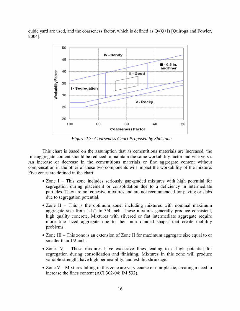
16

cubic yard are used, and the coarseness factor, which is defined as Q/(Q+I) [Quiroga and Fowler, 2004].

Figure 2.3: Coarseness Chart Proposed by Shilstone

This chart is based on the assumption that as cementitious materials are increased, the fine aggregate content should be reduced to maintain the same workability factor and vice versa. An increase or decrease in the cementitious materials or fine aggregate content without compensation in the other of these two components will impact the workability of the mixture. Five zones are defined in the chart:

• Zone I – This zone includes seriously gap-graded mixtures with high potential for segregation during placement or consolidation due to a deficiency in intermediate particles. They are not cohesive mixtures and are not recommended for paving or slabs due to segregation potential.

• Zone II – This is the optimum zone, including mixtures with nominal maximum aggregate size from 1-1/2 to 3/4 inch. These mixtures generally produce consistent, high quality concrete. Mixtures with slivered or flat intermediate aggregate require more fine sized aggregate due to their non-rounded shapes that create mobility problems.

• Zone III – This zone is an extension of Zone II for maximum aggregate size equal to or smaller than 1/2 inch.

• Zone IV – These mixtures have excessive fines leading to a high potential for segregation during consolidation and finishing. Mixtures in this zone will produce variable strength, have high permeability, and exhibit shrinkage.

• Zone V – Mixtures falling in this zone are very coarse or non-plastic, creating a need to increase the fines content (ACI 302-04; IM 532).

17

Percent Retained 2.5.5

The current ASTM C 33 specification could lead to poor workability mixtures and gap-graded mixtures due to an excess or a deficiency of some sizes. The goal of the “Percent Retained” method (Figure 2.4), sometimes referred to as the “18-8” method, is to produce uniform blends by limiting the maximum and minimum amount of aggregate fractions to a ceiling value of 18% and a floor value of 8% [Quiroga and Fowler, 2004].

A deficit in particles retained on the No. 8, 16 and 30 sieves and an excess of particles retained in the No. 50 and 100 sieves can be found in many areas of the U.S. This leads to problems such as cracking, curling, blistering, and spalling of concrete. If there is a deficit in one sieve but an excess on the adjacent sieve, the two sieve sizes can balance one another. However, if there are three adjacent deficient sieve sizes, the grading distribution in these sieves needs to be adjusted. These deficits can be seen through adjacent peaks and dips in the “18-8” chart [ACI 302-04; IM 532].

Figure 2.4: “18-8” Percent Retained Chart

This method, however, is not intended to be used for aggregate with high microfines content. The mixtures meeting the “18-8” limits could still have workability problems and low packing density due to an excess or deficit of either fine or coarse aggregate [Quiroga and Fowler, 2004].

18

19

Concrete Properties and Performance Literature Review Chapter 3.

The main acceptance criterion for aggregates should be related to their performance in concrete. If good quality concrete that meets all the required performance criteria can be made using a certain source of aggregate, then there is no reason not to use that aggregate. This chapter will discuss how aggregate properties affect fresh and hardened concrete performance. Methods of evaluating skid resistance and proportioning concrete are also reviewed in this chapter.

Effect of Fine Aggregates on Fresh Concrete Properties 3.1

Particle shape, texture, and grading have a great impact on the fresh properties of concrete. Mixtures containing high amounts of poorly shaped particles (like MFAs) tend to need a higher amount of paste content to achieve the same workability (compared to a mixture made with natural sands) [Fowler et al., 2008]. Other properties such as finishability, air content, bleeding, and segregation might also be affected by the use of MFA.

Workability 3.1.1

In the 1970s, an aggregate manufacturer in North Carolina began promoting the use of manufactured sands in pavement concrete. A test section was made with manufactured sand containing a maximum of 3% microfines. The performance of this manufactured sand was a nightmare for the paving contractor [Saunders, 1995]. The concrete workability was horrible; there was excessive bleeding, edge slump, and edge shearing [Saunders, 1995]. Following this incident, a 50/50 blend of manufactured sand and natural sand was used instead to improve performance.

Fine aggregates have a higher impact on workability than coarse aggregates [Wills, 1972]. One of the obstacles to using MFA in concrete is that manufactured sands are typically composed of sharp, angular particles with large numbers of flat and elongated particles [Graves, 2006]. Angular particles create a greater void volume within the aggregate. Additional paste (water and cement) is needed to fill those voids [Quiroga and Fowler, 2004]. This can be offset, however, by using a higher dosage of admixture [Fowler et al., 2008]. When using MFA in concrete mixtures, a water-reducing admixture may not be sufficient to achieve a slump of 2 in. [Trachet, 2008]. Mid-range or high-range water-reducing admixtures (MRWRA and HRWRA) have a higher water reducing capacity; however, MRWRA and HRWRA are not usually used for slipform paving jobs.

Another aspect of MFA that affects workability is the presence of high amounts of microfines. Microfines are believed to have an adverse effect on the workability of concrete due to their small sizes (large surface area) and because they might contain deleterious materials (like clay and other organic materials). Research by ICAR on self-consolidating concrete found that microfines can be successfully used and can lead to an improvement in the workability of concrete (when low amounts of deleterious materials such as clays are present) [Koehler and Fowler, 2007]. Furthermore, when microfines are considered as part of the aggregates, higher dosages of admixture are needed to achieve the same workability as compared to mixtures where the microfines are accounted for as part of the paste [Fowler et al., 2008].

Both the angular nature of MFA and the presence of high amount of microfines affect the workability of concrete. These negative impacts on workability can be counteracted by blending

20

sands, using an admixture, or by the addition of fly ash [Trachet 2008]. Increasing the quantity of manufactured sand in a blend will reduce workability or will require a higher dosage of admixture [Trachet, 2008].

Finishability 3.1.2

One of the problems experienced during the “TxDOT Implementation Project for Increased Microfines Content in Pavement Concrete” was problems that involved finishing [McLeroy, 2008]. The finishing crew tried to solve the problem by adding more water to the surface of the concrete (“blessing” the concrete). Such problems have not been encountered when natural sands were used, and are believed to have been caused due to the poor shape of MFA and the presence of high amounts of microfines [McLeroy, 2008]. A type D admixture (water reducing and retarding) was used in that project. Finishability can be improved by either improving the shape or grading of crushed aggregates [Saunders, 1995] or by using a different type of admixture. MRWRA admixtures have higher water reducing capacity, and have the ability to improve surface slickness, which results in easier finishing and better concrete surfaces [Schaefer, 1995]. Using a MRWRA might help solve workability and finishability problems encountered when MFA are used, but such admixtures are not usually used in paving concrete.

Bleeding and Segregation 3.1.3

By increasing the water demand, the amount of bleed water in the concrete increases [Washa, 1998; Kosmatka, 1994]. Research done during ICAR 401 [Fowler et al., 2008], have shown that for the same mixture proportions, mixtures containing MFA will only bleed if not enough paste (water and cement) is present in the mixture; the volume of paste to avoid bleeding in mixtures containing natural sands is lower than that of mixtures made with MFA. As for segregation, Kalcheff (1977), Hudson (1999), and research done by the Japan Society of Civil Engineers (2002), have shown that the presence of microfines help decrease the segregation of concrete.

Air Content 3.1.4

Research done during ICAR 104 suggest that the high percentage of microfines present in MFA can lead to an increase in the amount of entrained air, and thus decrease the amount of air-entrainment needed [Quiroga and Fowler, 2004]. Later research done on MFA has shown no correlations between the presence of MFA and the increase of entrained air [Trachet, 2008]. The observed increase in entrained air might be due to the increase in the dosage of the water-reducer, or maybe due to the presence of fly ash [Trachet, 2008].

The Effect of Fine Aggregates on Hardened Concrete Properties 3.2

The hardened properties of concrete are affected by the amount, mineralogy, and grading of aggregates. The addition of water to mixtures made with MFA to compensate for the water needed to achieve the required workability might affect the strength and durability. Properties that might be affected by the use of MFA include compressive and tensile/flexural strength, shrinkage, permeability, and skid resistance.

21

Strength 3.2.1

Using water-reducing admixtures, concrete mixtures made with MFA do not need additional water to achieve the required workability. ICAR 401 [Fowler el al. 2008] showed that the same compressive strength can be produced by using natural sand, a well-shaped manufactured sand, or a poorly-shaped manufactured sand. The only additional requirement was a higher dosage of admixture that was used to achieve the same workability. Research by Kim et al. (1997) has shown that concrete made with crushed limestone fines has generated compressive and tensile strengths about equal to or larger than natural sand. Other research by Celik and Marar (1996) has shown that the strength is affected by the percent of microfines in the sand; fine aggregates with amounts of microfines equal of about 30% lead to a decrease in compressive and flexural strength. For the same water-to-cement ratio, MFAs or blended sands demonstrate either equal or superior strength or resistance to carbonation, when compared to concrete made with natural sand [Yamamoto et al., 2005]. Using manufactured granite sand in a blend can cause reduction in compressive and flexural strength [Trachet, 2008], while using dolomitic limestone sand increases strength [Trachet, 2008]. The granite sand tested by Trachet (2008) produced concrete with the lowest values of compressive strength and flexural strength.

Shrinkage 3.2.2

Due to the restraining effect of aggregate particles, concrete generally shrinks less than cement paste. According to Torben el al. (1965), the degree of restraint provided by the aggregates in concrete is dependent on the quantity of aggregate, elastic properties of the aggregate, and the shrinkage of the cement paste and aggregate; the greater the volume of the aggregate in the concrete, the less the shrinkage. Furthermore, the lower the aggregate modulus of elasticity the lower the restraining effect on the cement paste during shrinkage. Higher shrinkage is usually associated with higher paste content (water and cement) [Fowler et al., 2008]. When microfines in manufactured sands are considered as part of the paste, rather than as part of the aggregates, shrinkage decreases; this is due to decrease of cement in the mixtures [Fowler et al., 2008]. Higher shrinkage in mixtures containing manufactured sands can be attributed to the higher paste requirements.

Skid Resistance 3.2.3

Skidding, slipping, or sliding occurs as a result of lack or loss of friction. Friction is defined as the force resisting relative motion of two objects in contact (Figure 3.1). Friction created by the tire and pavement interaction allows vehicles to accelerate, decelerate, and maneuver. A study done by Viner et al (2004) estimated that risks of accidents crashes can be halved by doubling the skid resistance [Hall et al., 2006]

22

Figure 3.1: Friction Force

In PCC pavements, adequate surface friction generally exists in dry conditions. In wet conditions the presence of water reduces the contact between the tire and the pavement, which reduces friction. If a sufficiently thick film of water is formed between the tire and the pavement (this might occur at higher traveling speeds), the tire will lose contact with the pavement, a phenomenon known as hydroplaning (Figure 3.2) [Hoerner et al., 2003]. The difference between hydroplaning and skidding is that in hydroplaning there is no contact between the tire and the road surface to develop any frictional force.

Figure 3.2: Hydroplaning

Early investigations of friction hypothesized that friction was only due to the interlocking of mechanical protuberances or asperities on the surfaces of contacting materials [Rabinowicz, 1995]. This explanation for the friction phenomena is referred two as the “roughness hypothesis” [Rabinowicz, 1995]. In the 1900s, as the science of surface chemistry was developed, it became evident that friction was not just due to roughness.

The friction force between two objects arises from the need to shear strongly adherent surface atoms of contacting materials [Rabinowicz, 1995]. This phenomenon is known as adhesion and usually accounts for 90% or more of the overall friction force [Rabinowicz, 1995]. On wet pavements, adhesion can account for two-thirds of the resistance force [Hogervorst, 1974]. The other main factor contributing to the frictional force involves the roughness of a surface [Rabinowicz, 1995]. This component of friction arises from the need during the sliding

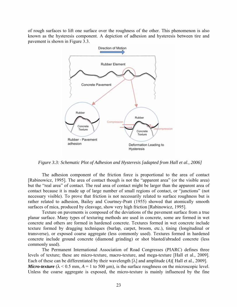
23

of rough surfaces to lift one surface over the roughness of the other. This phenomenon is also known as the hysteresis component. A depiction of adhesion and hysteresis between tire and pavement is shown in Figure 3.3.

Figure 3.3: Schematic Plot of Adhesion and Hysteresis [adapted from Hall et al., 2006]

The adhesion component of the friction force is proportional to the area of contact [Rabinowicz, 1995]. The area of contact though is not the “apparent area” (or the visible area) but the “real area” of contact. The real area of contact might be larger than the apparent area of contact because it is made up of large number of small regions of contact, or “junctions” (not necessary visible). To prove that friction is not necessarily related to surface roughness but is rather related to adhesion, Bailey and Courtney-Pratt (1955) showed that atomically smooth surfaces of mica, produced by cleavage, show very high friction [Rabinowicz, 1995].

Texture on pavements is composed of the deviations of the pavement surface from a true planar surface. Many types of texturing methods are used in concrete, some are formed in wet concrete and others are formed in hardened concrete. Textures formed in wet concrete include texture formed by dragging techniques (burlap, carpet, broom, etc.), tining (longitudinal or transverse), or exposed coarse aggregate (less commonly used). Textures formed in hardened concrete include ground concrete (diamond grinding) or shot blasted/abraded concrete (less commonly used).

The Permanent International Association of Road Congresses (PIARC) defines three levels of texture; these are micro-texture, macro-texture, and mega-texture [Hall et al., 2009]. Each of these can be differentiated by their wavelength [λ] and amplitude (A)[ Hall et al., 2009]. Micro-texture (λ < 0.5 mm, A = 1 to 500 μm), is the surface roughness on the microscopic level. Unless the coarse aggregate is exposed, the micro-texture is mainly influenced by the fine

24

aggregate in PCC pavements. The micro-texture is important to maintain adequate friction in dry-weather conditions and wet-weather conditions when speeds are under 72 km/h (45 mph) [Hall et al., 2009]. Macro-texture (0.5 mm ≤ λ < 50 mm, A = 0.1 to 20 mm) is defined by the type of surface finishing/texturing technique formed in the surface of the concrete. Good macro-texture is required to maintain adequate friction under wet-weather conditions at speeds over 72 km/h (45 mph) and to prevent hydroplaning. Mega-texture (50 mm ≤ λ < 500 mm, A = 0.1 to 50 mm). This type of texture is usually undesirable and is unintentionally formed or is a result for distress in concrete.

Texture can also influence properties of the pavement other than friction. These properties include noise, ride quality, splash and spray and tire wear. A summary of how the different levels of texture can affect concrete pavement is presented in Figure 3.4. In Figure 3.5, aggregate texture, fine aggregate size, and coarse aggregate size are compared to the wavelength of the different levels of texture on a pavement.

Figure 3.4: Pavement Wavelength and Surface Characteristics [adapted from Hall et al., 2006;

Hoerner, 2003]

Micro-texture Macro-texture Mega-texture Roughness/Unevenness

10-6 m 5 x 10-3 m 5 x 10-2 m 5 x 10-1 m 10 m

4 x 10-4 in. 2 x 10-2 in. 2 in. 20 in. 300 in.

Aggregate Texture

Fine Aggregate

Coarse Aggregate

Surface channels, grooves, or indentations

that are intentionally formed

Figure 3.5: Type of Texture Contributing to Texture

25

After the texture formed on the concrete surface is abraded (mainly the texture created by dragging techniques), the skid resistance of a pavement is a function of the fine aggregate used in the concrete mixture. This property of PCC pavement was recognized early on and research has been done to find tests that better evaluate the performance of fine aggregates for skid.

According to Balmer and Colley (1966), the need for skid resistant pavements was recognized in 1958 by the First International Skid Prevention Conference. After this conference, state agencies started to develop equipment to test skid both in the laboratory and in the field. In 1958, Shupe and Lounsbury showed a correlation between calcium carbonate content of aggregates and skidding susceptibility. Gray and Renninger (1965) recognized the contribution of siliceous sand particles in skid resistance and pioneered the AI test to analyze the amount of siliceous materials in the aggregates. Balmer and Colley (1966) compared AI of fine aggregates to a laboratory skid performance test. It should be noted, however, that the acid insoluble test used by Balmer and Colley differed significantly from what is currently being used by TxDOT. Balmer and Colley tested samples that had a weight ranging from 1 to 2 lbs. (450 to 900 grams) with a 6N solution of hydrochloric acid solution. The TxDOT test method uses 25 grams of fine aggregates along with a concentrated hydrochloric acid solution. ASTM D 3042 (Standard Test Method for Insoluble Residue in Carbonate Aggregates) is similar to the test conducted by Balmer and Colley.

The laboratory testing conducted by Balmer and Colley consisted of subjecting concrete specimen made with sands having different mineralogy to three cycles of wear. The first and third cycles consisted of wearing the surface by means of a rotating 600 lb loaded tire. The second cycle was similar to the first and third cycles, but was complemented by the addition of fine Ottawa sand. The goal of adding the fine aggregate was to simulate wear caused by the grit and dirt on roadways. The results obtained from Balmer and Colley are shown in Table 3.1.

26

Wear Index Results Obtained by Balmer and Colley (1966) Table 3.1:

Balmer and Colley rated the skid performance of the concrete by measuring the power

required to rotate a wheel against the abraded specimen. This value was translated into a wear index. The wear index values ranged from 3.5 to 7.5 (Table 3.1); the “calcites” (probably limestone aggregates) had the lowest values, while the aggregates containing quartz (siliceous) had the highest. Although dolomitic aggregates were rated as “poor,” they had values ranging from 4.4 to 5.8.

After comparing the results obtained from the aggregate tests to the concrete laboratory performance test, Balmer and Colley concluded that 25% siliceous fine aggregate replacement was satisfactory for performance with most aggregates (Figure 3.6).

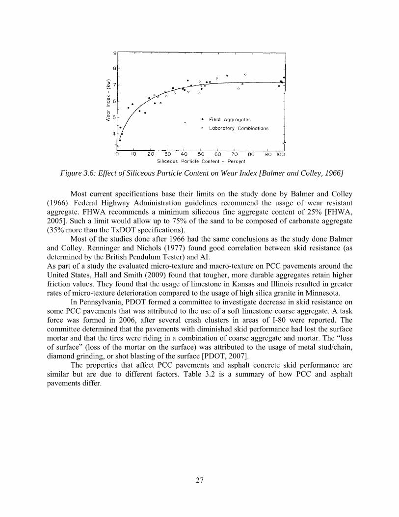
27

Figure 3.6: Effect of Siliceous Particle Content on Wear Index [Balmer and Colley, 1966]

Most current specifications base their limits on the study done by Balmer and Colley (1966). Federal Highway Administration guidelines recommend the usage of wear resistant aggregate. FHWA recommends a minimum siliceous fine aggregate content of 25% [FHWA, 2005]. Such a limit would allow up to 75% of the sand to be composed of carbonate aggregate (35% more than the TxDOT specifications).

Most of the studies done after 1966 had the same conclusions as the study done Balmer and Colley. Renninger and Nichols (1977) found good correlation between skid resistance (as determined by the British Pendulum Tester) and AI. As part of a study the evaluated micro-texture and macro-texture on PCC pavements around the United States, Hall and Smith (2009) found that tougher, more durable aggregates retain higher friction values. They found that the usage of limestone in Kansas and Illinois resulted in greater rates of micro-texture deterioration compared to the usage of high silica granite in Minnesota.

In Pennsylvania, PDOT formed a committee to investigate decrease in skid resistance on some PCC pavements that was attributed to the use of a soft limestone coarse aggregate. A task force was formed in 2006, after several crash clusters in areas of I-80 were reported. The committee determined that the pavements with diminished skid performance had lost the surface mortar and that the tires were riding in a combination of coarse aggregate and mortar. The “loss of surface” (loss of the mortar on the surface) was attributed to the usage of metal stud/chain, diamond grinding, or shot blasting of the surface [PDOT, 2007].

The properties that affect PCC pavements and asphalt concrete skid performance are similar but are due to different factors. Table 3.2 is a summary of how PCC and asphalt pavements differ.

28

Properties and Factors Affecting the Skid Resistance of PCC and Asphalt Table 3.2:Pavements

Property/Factor PCC Pavement Asphalt Concrete Pavement

Aggregates contributing to skid resistance

Unless the coarse aggregate is exposed, skid resistance is mainly affected by the fine

aggregate.

The coarse aggregate plays a major role in skid resistance; fine aggregate have little to

no effect.

Aggregate property affecting skid resistance

Fine aggregate mineralogy is the main factor in determining the long-term skid resistance

of PCC pavements.

Coarse aggregate mineralogy, shape, angularity, and texture

affect performance.

Macro-texture

Macro-texture is formed on the concrete surface to drain the pavement from water and to avoid hydroplaning; it is formed mainly by tining or

grooving.

Macro-texture is not intentionally formed; it is

defined by the angularity and shape of the coarse aggregate.

Loss of skid (deterioration)

Wear or loss of friction is mainly due to abrasion.

Other factors might affect the loss of skid resistance besides

abrasion (such as temperature, age, etc.).

Evaluating Pavement Skid Performance 3.3

Many methods have been developed to evaluate skid resistance both for field and laboratory usage. These methods either evaluate micro-texture, macro-texture, or both. In this section, methods of evaluating friction, texture, and equipment used to simulate wear at a laboratory will be discussed.

Test Methods for Evaluating Texture 3.3.1

The Sand Patch Method (ASTM E 965 or Tex-436-A) is a method used to measure the average macro-texture depth of a pavement. The test consists of spreading a uniform material of known volume on a clean and dry pavement surface and then calculating the average depth of the macro-texture based on the area covered by the material. The sand test method is known to be cumbersome and has poor repeatability [Doty, 1974]. Another method similar to the sand patch method was developed, it is known as the grease patch method.

The Outflow Meter (ASTM E 2380) is also a method used to evaluate macro-texture. It consists of measuring the time it takes for a cylinder of known volume to discharge water over a pavement. This method is suitable as a field test to evaluate surface drainage.

The Circular Track Meter (CTM) (ASTM E 2157) is a device that utilizes a displacement sensor that is mounted on an arm that rotates in a circular path and measures the mean profile depth (MPD) of a pavement (macro-texture). The CTM is a device that can be used in the field and in a laboratory to evaluate macro-texture.

Many other methods that use laser or image processing equipment like the CTM have been developed. Some of these include the Road Surface Analyzer (ROSAN), Robotex, the

29

Multi-Laser Profiler (MLP), the Lightweight Profiler, and the Liteweight Inertial Surface Analyzer (LISA). Many of those devices were developed because highway agencies were researching methods of evaluating pavement texture and skid resistance without interrupting traffic.

Test Methods for Evaluating Friction 3.3.2

The Locked-Wheel Skid Trailer (ASTM E 274) is the most common method used by state agencies to evaluated skid resistance. The method consists of measuring the locked-wheel friction (100% slip condition) of a trailer towed behind a truck at a speed of 40 mph (TxDOT uses 50 mph). The trailer administers a water spray to the pavement in front of the tire to simulate wet conditions. The resulting friction force acting between the test tire and the pavement surface is used to determine the skid resistance which is reported as a skid number (SN). Higher SN values signify higher skid resistance. A smooth tire (ASTM E 524) or a ribbed tire (ASTM E 501) can be used on the skid trailer. Research has shown that ribbed tires are only capable of evaluating the effect of micro-texture on friction, while smooth tires can measure the contribution of micro-texture as well as macro-texture [Jackson, 2008; Hall et al., 2006]. Some state agencies have trigger skid values that they use as means of initiating some sort of rehabilitation treatment; these values differ from state to state. The most common trigger values reported are SN < 35 or 30 for ribbed tires, and SN < 20 for smooth tires [Hall et al., 2006]. It is believed that SN values below those limits can result in an increase in skid related accidents on roadways.

The British Pendulum Tester (BPT) (ASTM E 303) is one of the simplest and cheapest instruments used in the measurement of friction characteristics of pavement surfaces [Lee, 2005].The BPT produces a low-speed sliding contact (about 6 mph, or 10 km/hr) between a standard rubber slider and a pavement surface. The elevation to which the arm swings after contact is used to compute a frictional value. Various studies have shown that the BPT is unreliable especially when used on coarse-textured surfaces [Lee, 2005].

The Dynamic Friction Tester (DFT) (ASTM E 1911) is laboratory and field apparatus that measures the friction-speed relationship on a pavement surface for speeds ranging from 0 to 50 mph (80 km/hr). The DFT measures the torque needed to stop three small spring-loaded standard rubber pads rotating in a circular path. The torque measured is then converted to a friction value. Water is also introduced during testing to simulate wet conditions. The DFT can be used along with the CTM to evaluate both micro-texture and macro-texture on the same circular path.

Since the 1960s many methods of measuring frictional resistance have been invented worldwide. Most of these methods were mainly developed for field usage and they closely resemble the Locked-Wheel Skid Trailer discussed earlier; these include the British Mu-Meter, the British Sideway Force Coefficient Routine Investigation Machine (SCRIM), Roadway and runway friction testers (RFTs), the Airport Surface Friction Tester (ASFT), the Saab Friction Tester (SFT), the Griptester, the Finland BV-11, the Road Analyzer and Recorder (ROAR), and the Norwegian Norsemeter RUNAR [Hall et al., 2006]. Other methods of evaluating friction are based on measuring the stopping distance (ASTM E 445) or the deceleration rate (ASTM E 2101). Some of these methods are used to evaluate friction at different speeds while an antilock braking system (ABS) is fully engaged. Laboratory sized equipment similar to the BPT and DFT have also been developed; these include the Michigan Laboratory Friction Tester, the North

30

Carolina Variable Speed Friction Tester, and the Pennsylvania Transportation Institute (PTI) Tester.

Accelerated Wear and Polishing Devices 3.3.3

Machines that simulate wear and polish caused by traffic have been used since research on skid resistance started in the 1960s. Some were made to wear and polish aggregates, while others were made to wear and polish asphalt and concrete surfaces. Such devices include

• The British Polishing Wheel.

• The Michigan Indoor Wear Track.

• The MD.

• The Three-Wheel Polishing Device (TWPD) developed by the National Center for Asphalt Technology (NCAT).

• The North Carolina State University Wear and Polishing Machine.

• The Wehner/Schulze Polishing Machine.

• The Penn State Reciprocating Polishing Machine.

• The Model Mobile Load Simulator (MMLS-3).

All those machines essentially do the same thing; they wear and polish aggregate, asphalt, or concrete surfaces. In general these devices differ in the following:

• The size of the machine and the area it polishes.

• The material used to polish specimen (Different types of tire material have been used to abrade the surfaces).

• Some devices have used means to accelerate wearing and polishing. For example, hard sands have been used to complement and accelerate the wear caused by tires.

• Some devices utilize water in the abrasion process, while others do not. It should be noted that most of those devices have been developed for testing asphalt

pavements and not for concrete pavements. Moreover, some of those devices have shown to reproduce wearing and polish patterns very similar to what is observed in the field; such machines can be used to estimate when the loss of skid will occur based on the materials used, expected traffic, and age of a pavement.

Correlating Skid Values Measured by Different Devices 3.3.4

Many methods and devices of evaluating skid resistance have been created, and each of these evaluates skid in its own defined way. The need to define a common scale for friction on pavements was explored by the Permanent International Association of Road Congresses (PIARC). In 1992, PIARC conducted a study aimed at correlating the results obtained from 51 different measurement systems used worldwide. Sixteen countries covering each continent participated and experiments were conducting at 54 sites across the U.S and Europe. One of the

31

main results of the PIARC experiment was the development of the International Friction Index (IFI) [PIARC, 1995]. ASTM E 1960 defines the IFI as an index for comparing and harmonizing friction measurements with different equipment to a common calibrated index. For example values measured using a CTM and DFT can be used to calculate the IFI index; the IFI index can then be used to compute the equivalent texture or friction values for other devices. The following is an example of how values measured using a CTM and DFT can be converted to equivalent locked-wheel skid trailer SNs (ASTM E 274):

• The IFI parameters F60 and Sp are first computed using the formulas provided in ASTM 1960: = 14.2 + 89.7 (Eq. 3.1) 60 = + × × ( )⁄ (Eq. 3.2)

• A and B are the calibrated constants for the device used for measurement: A = 0.0082 and B = 0.732 for the coefficient of friction measured by the DFT at 12 mph (20 km/hr) (ASTM 1960). FRS is the friction value measured at a speed S (in this case at 20 km/hr). The MPD is the mean profile depth value measured by the CTM. 60 = 0.081 + 0.732 ⁄ (Eq. 3.2)

• After the IFI parameters F60 and Sp are computed, the same formulas using different device constants can be used to compute the equivalent friction.

• To compute the equivalent SN measured by a locked-wheel skid trailer at 50 mph using a smooth tire (ASTM E 524), the following formula can be used:

(50) = .. × . × 100 (Eq. 3.3)

• To compute the equivalent SN measured by a locked-wheel skid trailer at 40 mph using a ribbed tire (ASTM E 501), the following formula can be used:

(40) = . . ×. × . × 100 (Eq. 3.4)

Research done at University of North Florida on asphalt concrete found direct correlation

between the DFT coefficient of friction at 37 mph (60 km/hr) and the locked-wheel skid trailer value measured at 40 mph using ribbed tires [Jackson, 2008]. A similar correlation for asphalt concrete was found by NCAT after correlating field and laboratory results (Figure 3.7) [Heitzman, 2011].

32

Figure 3.7: Correlation between SN(64)ribbed and DFT60 (metric units) [Heitzman, 2011]

Diamond Grinding and Grooving 3.4

Diamond grinding is a technique used to correct irregularities or restore surface friction on PCC pavements and bridges. Grinding consists of cutting the surface of a hardened concrete pavement using closely spaced saw blades. Grooving involves cutting the pavement with deeper cuts that serve as water channels which help drain the pavement and prevent hydroplaning.

Grinding a surface restores macro-texture initially increasing the surface friction. However, the concern with grinding is that the increase in friction will be short-lived if a soft aggregate is exposed. The texture produced by grinding varies depending on the size of blades used on the grinding head. Larger spacers produce larger land areas, while smaller spacers produce smaller land areas (Figure 3.8).

Figure 3.8: Factors Affecting Diamond-Ground Surfaces

Compared to other repair techniques, grinding has many advantages, including the following:

• Improvements in ride quality by making the concrete surface smoother.

• Possible reduction in noise on pavements. Research on noise has focused on finding the optimum blade configuration to produce the quietest pavement.

Grinding operations do not require shutting down adjacent lanes; they require less traffic

interruptions than other restoration techniques. Moreover, using multiple machines during a grinding operation allows a lane to be completed and opened to traffic after only one pass.

33

Mix Proportioning Methods for Portland Cement Concrete 3.5

Many approaches to mix proportioning have been published; most are based on the following principals:

• Fineness modulus

• Void density

• Specific surface

• Workability factor Since most of the research done by ICAR at University of Texas at Austin attempted to find better methods of proportioning manufactured aggregates in concrete, only two methods for proportioning concrete were considered and evaluated during this research project. The first method is the ACI method (ACI 211), and the second is the proportioning method developed by ICAR that was made specifically for proportioning manufactured sands in concrete.

ACI Mixture Design Method 3.5.1

The ACI 211 (2002) method is based on an empirical formula that indirectly determines the amount of aggregates in a mixture. The values recommended by ACI assume that the aggregates are well graded and no guidance is given on how to blend two or more aggregates.

The ACI method relates the amount of cement needed in a mixture to strength and durability criteria in terms of minimum amount of cement and required water-to-cement ratio (w/c). The amount of water required increases with increasing aggregate angularity, increasing slump, decreasing maximum aggregate size, lack of air entrainment, or use of water-reducing admixtures. The volume of coarse aggregate is a function of the dry-rodded unit weight of the coarse aggregate, the fineness modulus of the fine aggregate, and the maximum aggregate size. The volume of fine aggregates depends on the amount of all other ingredients.

One of the major shortcomings of the ACI approach is that it over simplifies the proportioning process by using the fineness modulus of the sand as a factor. Research done by Young (1921), Besson (1935), and Kennedy (1940) suggest that the fineness modulus is inadequate to differentiate between sands. ACI also relates strength and durability of concrete to cement content (by specifying a minimum cement content), which is also misleading. Furthermore, ACI 211 is based on ASTM C 33 which limits the amount of microfines to a maximum of 7%.

ICAR Method for Proportioning Concrete 3.5.2

The ICAR method was originally developed by Fowler and Koehler (2007) for self-consolidating concrete and was then modified by McLeroy (2009) for pavement concrete. Following are the recommended steps for designing a mixture containing MFA:

1. Choose the aggregate system.

• Evaluate aggregate properties.

• Determine optimum grading.

34

2. Choose the paste quantity.

• Determine minimum paste content based on the chosen combined aggregate gradation.

• Determine additional paste needed for workability based on shape and angularity of MFA.

3. Choose the paste quality.

• Choose the type of Supplementary Cementitious Materials (SCM).

• Choose air content.

• Choose w/cm. Each item is discussed in more details in the following section.

1. Choosing the Aggregate System

To improve the performance of concrete, it is important to properly choose aggregates based on the properties obtained from characterization tests. Each of the characterization tests has been developed to evaluate critical aggregate properties that influence concrete performance.

To achieve the highest packing density of aggregates, more than one grade of aggregate can be used. The combined gradation of coarse and fine aggregate should be evaluated using a modified 0.45 power curve. The modified 0.45 power curve should not take into account the presence of microfines since the microfines will be accounted for as part of the paste not the aggregate. The modified 0.45 power curve should go through the #200 sieve (Figure 3.9).

Figure 3.9: Modified 0.45 Power Curve (Fowler and Koehler 2007)

In addition to using a modified 0.45 power curve, two other methods can be used to ensure that uniform blends of aggregates are being used: the 8-18 grading system and the Shilstone Coarseness chart. Note that Fowler and Quiroga (2004) found that the 8-18 grading system was not suitable for evaluating aggregates with high microfine content.

After the optimal grading is determined using the modified 0.45 power curve, the dry-rodded unit weight (DRUW) of the aggregate combination should be evaluated (the Tex-404-A - rodded method can be used). To ensure that highest aggregate density was obtained, multiple

35

aggregate combinations can be tested using the modified 0.45 power curve and then by obtaining the DRUW; the combination with the highest DRUW corresponds to the highest aggregate density.

After obtaining DRUW, the percent compacted voids corresponding to the chosen aggregate gradation should be determined. The percent compacted void content is determined as follows: % _ = 1 − ( . )∑ ( ( ) ) × 100% (Eq. 3.5)

where DRUW is the dry-rodded unit weight of the combined aggregate (lb/ft3), pi is the volume of aggregate fraction i divided by the total aggregate volume, and (SGOD)i is the oven-dry specific gravity of aggregate fraction i.

2. Choosing the Paste Quantity

Figure 3.10 shows a schematic representation of aggregate in cement paste. The total volume of paste needed for concrete is equal to the volume of paste needed to fill the voids in compacted aggregates + the volume of paste needed to separate aggregate.

Figure 3.10: Paste Needed to Fill Voids between Aggregates [Koehler and Fowler, 2007]

spacingpasteVoidspastepasteTotal VVV _+= − (Eq. 3.6)

VoidspasteV − corresponds to the aggcompactedVoids _% calculated using DRUW. spacingpasteV _ is related to

the shape and angularity of fine aggregate. Fowler and McLeroy (2009) found that spacingpasteV _

for a class P concrete containing high microfines content ranges from 3 to 8% paste by volume.

3. Choosing the Paste Quality

After the paste quantity is determined, the composition of the paste is selected to achieve the required plastic and hardened concrete properties. The paste is composed of cement, water, SCMS, air, mineral fillers (microfines present in the fine aggregates are accounted as mineral fillers), and admixtures. Table 3.3 summarizes the effect and purpose of the different paste constituents.

36

Selection of Paste Composition [Fowler and Koehler 2007] Table 3.3:

37

Material Properties Chapter 4.

The main goal of this research project was to evaluate the properties of fine aggregates in PCC pavement. To do so, other materials were also needed, such as cementitious materials, admixtures, and coarse aggregates. This chapter presents a list of materials used on this project as well as the results for all standard tests for fine and coarse aggregates.

Cementitious Material and Admixtures 4.1

The cement used for all mortar and concrete mixtures was an ASTM C 150 Type I/II cement obtained from TXI Midlothian; this cement is used in the Dallas and Fort Worth Districts. A class F fly from Boral Material Technologies was used for the six blended sand mixtures tested for skid resistance (discussed in a later chapter). Fly ash was added to those mixtures to test blended mixtures that better represent those used in the field.

TxDOT required that the fine aggregates be evaluated for skid resistance using identical concrete mixture proportions. Thus, a mid-range water reducing admixture was used to facilitate the casting of concrete specimens. DARACEM 55 was used to make specimens that were tested for strength, modulus of elasticity, skid resistance, and shrinkage. DARACEM 55 is a mid-range water-reducing admixture produced by W.R. Grace. This type of admixture is not common for slipform paving mixtures and was used only to evaluate hardened concrete properties. To evaluate concrete proportions for workability (slump), WRDA 82 was used. WRDA 82 is an ASTM C 494 Type A and D admixture produced by W.R. Grace.

Fine Aggregates 4.2

Thirty-three fine aggregates were tested in this project. Nine of the fine aggregates were natural siliceous fine aggregates and were chosen based either on their AI values or because they are materials local to the Dallas and Fort Worth Districts. The following is a list of the natural sands that were evaluated:

• TXI Paradise

• Trinity Kopperl

• Chanas Eagles Nest

• Lattimore Cleburne

• Grandbury Pit #1

• Ingram Rainbow

• Lattimore Rosser

• TXI Beckett Rd.

• Colorado River Sand Twenty MFAs were tested; some were chosen based on their mineralogy while others were

selected because they are materials local to the Dallas and Fort Worth district. These MFAs included the following:

38

• Lattimore Materials - Stringtown (slate)

• Martin Marietta Materials Apple (sandstone)

• Capital Aggregates - Marble Falls (dolomite)

• Cemex West Quarry (dolomite)

• Cemex South Quarry (dolomite)

• Cemex McKellingon (dolomite)

• Ingram Del Rio (dolomite)

• Alamo Evans Road (limestone)

• Martin Marietta Materials Centerpoint (limestone)

• Martin Marietta Materials New Braunfels (limestone)

• Martin Marietta Materials Beckman (limestone)

• Mummie Mummie (limestone)

• Cemex Balcones (limestone)

• South West Aggregate Knipa (limestone)

• Ingram Hondo (limestone)

• Yarrington Road (limestone)

• Colorado Materials Hunter (limestone)

• Texas Crushed Stone-Feld Pit (limestone)

• TXI Bridgeport (limestone)

• Hanson Servtex (limestone)

• Hanson Perch Hill (limestone)

• Vulcan Materials Hebner (limestone)

• Vulcan Materials Helotes (limestone)

• Vulcan Materials 1604 (limestone) The types of fine aggregates used are referred to as siliceous, limestone, dolomite,

sandstone, or slate. The lithology of those rocks was determined by the TxDOT petrographer. For the purpose of this project, evaluating the mechanical properties of the sands was determined to be more important than evaluating the exact mineral composition. To evaluate those properties, these ASTM or TxDOT standard tests were used:

• Sieve analysis (Tex 401-A)

• Specific gravity and absorption (Tex 403-A & ASTM C 128)

• DRUW (Tex 404-A)

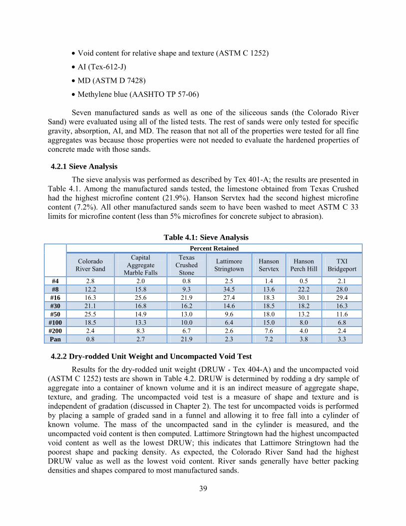
39

• Void content for relative shape and texture (ASTM C 1252)

• AI (Tex-612-J)

• MD (ASTM D 7428)

• Methylene blue (AASHTO TP 57-06) Seven manufactured sands as well as one of the siliceous sands (the Colorado River

Sand) were evaluated using all of the listed tests. The rest of sands were only tested for specific gravity, absorption, AI, and MD. The reason that not all of the properties were tested for all fine aggregates was because those properties were not needed to evaluate the hardened properties of concrete made with those sands.

Sieve Analysis 4.2.1

The sieve analysis was performed as described by Tex 401-A; the results are presented in Table 4.1. Among the manufactured sands tested, the limestone obtained from Texas Crushed had the highest microfine content (21.9%). Hanson Servtex had the second highest microfine content (7.2%). All other manufactured sands seem to have been washed to meet ASTM C 33 limits for microfine content (less than 5% microfines for concrete subject to abrasion).

Sieve Analysis Table 4.1:

Percent Retained

Colorado River Sand

Capital Aggregate

Marble Falls

Texas Crushed

Stone

Lattimore Stringtown

Hanson Servtex

Hanson Perch Hill

TXI Bridgeport

#4 2.8 2.0 0.8 2.5 1.4 0.5 2.1 #8 12.2 15.8 9.3 34.5 13.6 22.2 28.0 #16 16.3 25.6 21.9 27.4 18.3 30.1 29.4 #30 21.1 16.8 16.2 14.6 18.5 18.2 16.3 #50 25.5 14.9 13.0 9.6 18.0 13.2 11.6

#100 18.5 13.3 10.0 6.4 15.0 8.0 6.8 #200 2.4 8.3 6.7 2.6 7.6 4.0 2.4 Pan 0.8 2.7 21.9 2.3 7.2 3.8 3.3

Dry-rodded Unit Weight and Uncompacted Void Test 4.2.2

Results for the dry-rodded unit weight (DRUW - Tex 404-A) and the uncompacted void (ASTM C 1252) tests are shown in Table 4.2. DRUW is determined by rodding a dry sample of aggregate into a container of known volume and it is an indirect measure of aggregate shape, texture, and grading. The uncompacted void test is a measure of shape and texture and is independent of gradation (discussed in Chapter 2). The test for uncompacted voids is performed by placing a sample of graded sand in a funnel and allowing it to free fall into a cylinder of known volume. The mass of the uncompacted sand in the cylinder is measured, and the uncompacted void content is then computed. Lattimore Stringtown had the highest uncompacted void content as well as the lowest DRUW; this indicates that Lattimore Stringtown had the poorest shape and packing density. As expected, the Colorado River Sand had the highest DRUW value as well as the lowest void content. River sands generally have better packing densities and shapes compared to most manufactured sands.

40

Dry-Rodded Unit Weight and Uncompacted Voids Table 4.2:

Colorado

River Sand

Capital Aggregate

Marble Falls

Texas Crushed

Stone

Lattimore Stringtown

Hanson Servtex

Hanson Perch Hill

TXI Bridgeport

DRUW (lb/ft3) 108 105.8 105.6 102.2 106.7 106.2 106.1 Uncompacted

Voids (%) 39.4 46.4 47.6 48.0 43.7 44.3 44.2

Methylene Blue Test 4.2.3

The methylene blue test was conducted based on the procedures described in AASHTO TP 57-06 (only the aggregates passing No.200 sieve were tested). The methylene blue test indicates the presence of clay-like material in the aggregate. The results are shown in Table 4.3. All the fine aggregates were expected to perform well in concrete except for the Colorado River Sand. Although the test results indicate that that sand is marginally acceptable, the sieve analysis results indicate that the percent aggregates passing the No.200 sieve was 0.8% (Table 4.1). Thus the presence of clay in the microfines of the Colorado River Sand should not be an issue.

Methylene Blue Value (MBV) Table 4.3:

Colorado

River Sand

Capital Aggregate

Marble Falls

Texas Crushed

Stone

Lattimore Stringtown

Hanson Servtex

Hanson Perch Hill

TXI Bridgeport

MBV Value (mg/g)

10.25 4.00 5.50 3.0 6.50 3.50 3.00

Specific Gravity, Absorption, Acid Insoluble Residue, and Micro-Deval 4.2.4

The results for specific gravity, absorption, AI (discussed in Section 2.1), and MD (discussed in Section 2.2) for all the manufactured sands are presented in Table 4.4; the results for the siliceous sands are presented in Table 4.5.

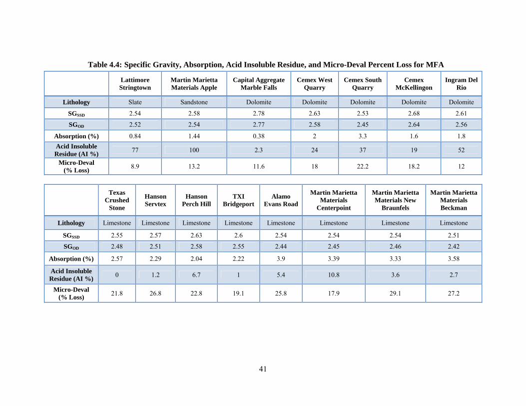
41

Specific Gravity, Absorption, Acid Insoluble Residue, and Micro-Deval Percent Loss for MFA Table 4.4:

Lattimore Stringtown

Martin Marietta Materials Apple

Capital Aggregate Marble Falls

Cemex West Quarry

Cemex South Quarry

Cemex McKellingon

Ingram Del Rio

Lithology Slate Sandstone Dolomite Dolomite Dolomite Dolomite Dolomite

SGSSD 2.54 2.58 2.78 2.63 2.53 2.68 2.61

SGOD 2.52 2.54 2.77 2.58 2.45 2.64 2.56

Absorption (%) 0.84 1.44 0.38 2 3.3 1.6 1.8

Acid Insoluble Residue (AI %)

77 100 2.3 24 37 19 52

Micro-Deval (% Loss)

8.9 13.2 11.6 18 22.2 18.2 12

Texas Crushed

Stone

Hanson Servtex

Hanson Perch Hill

TXI Bridgeport

Alamo Evans Road

Martin Marietta Materials

Centerpoint

Martin Marietta Materials New

Braunfels

Martin Marietta Materials Beckman

Lithology Limestone Limestone Limestone Limestone Limestone Limestone Limestone Limestone

SGSSD 2.55 2.57 2.63 2.6 2.54 2.54 2.54 2.51

SGOD 2.48 2.51 2.58 2.55 2.44 2.45 2.46 2.42

Absorption (%) 2.57 2.29 2.04 2.22 3.9 3.39 3.33 3.58

Acid Insoluble Residue (AI %)

0 1.2 6.7 1 5.4 10.8 3.6 2.7

Micro-Deval (% Loss)

21.8 26.8 22.8 19.1 25.8 17.9 29.1 27.2

42

Mummie Mummie

Cemex Balcones

South West Aggregate

Knipa

Ingram Hondo

Yarrington Road

Colorado Materials

Hunter

Vulcan Materials Hebner

Vulcan Materials Helotes

Vulcan Materials

1604

Lithology Limestone Limestone Limestone Limestone Limestone Limestone Limestone Limestone Limestone

SGSSD 2.64 2.62 2.6 2.62 2.57 2.57 2.53 2.5 2.58

SGOD 2.60 2.58 2.55 2.57 2.49 2.50 2.47 2.41 2.53

Absorption (%) 1.5 1.7 1.9 1.88 3.1 2.6 2.27 3.5 2.06

Acid Insoluble Residue (AI %)

8.1 4 21 8 5 4.5 6.4 10.7 3.6

Micro-Deval (% Loss)

17.1 29.7 15.7 16.6 20.5 28.3 24.8 33.4 22.4

Specific Gravity, Absorption, Acid Insoluble Residue, and Micro-Deval Percent Loss for Siliceous Sands Table 4.5:

TXI

Paradise Colorado

River Sand TXI

Beckett Rd.Eagle’s

Nest Ingram

Rainbow Lattimore Cleburne

Lattimore Rosser

Trinity Kopperl

Granbury Pit #1

Lithology Siliceous Siliceous Siliceous Siliceous Siliceous Siliceous Siliceous Siliceous Siliceous SGSSD 2.65 2.60 2.67 2.63 2.63 2.63 2.67 2.64 2.64 SGOD 2.64 2.58 2.64 2.62 2.62 2.62 2.65 2.63 2.61

Absorption (%) 0.62 0.45 0.77 0.6 0.52 0.58 0.79 0.68 1.11 Acid Insoluble Residue (AI %)

74.4 84.5 77 95.3 85.9 72.6 73.6 76.8 98

Micro-Deval (% Loss)

8.2 7.7 6.5 7.6 8.3 7.1 6.4 6.8 3.5

43

At least two specific gravity and absorption tests were performed on each aggregate, but

only one value was reported in Table 4.5 (the other values were used to check that the reported value was in the same range). Two AI tests and at least two MD tests were performed on each aggregate.

The values obtained for specific gravity, absorption, AI, and MD for all the siliceous sands are not significantly different. The absorption values for the limestone sands were higher than for all of the other sands tested. One of the dolomite sands and the slate sand had absorption values closer to the values of the siliceous sands. All carbonate aggregates failed the AI test (did not meet the 60% limit). Compared to the other carbonate aggregates, the Capital Marble Falls (dolomite) and Ingram Del Rio (dolomite) had lower MD percent loss. As for the limestone aggregates, the MD percent loss had a wide range that varied from 15.7 to 33.4%, the lowest percent loss for limestones was obtained for South West Aggregate Knipa. The MD percent loss for the siliceous sands ranged from 3.5 to 8.2%.

Coarse Aggregates 4.3

Four coarse aggregates were used in this project; two were limestone coarse aggregates that were used for all mixture proportioning and fine aggregate skid testing, while the other two were only used for diamond grinding tests. All the coarse aggregates used were TxDOT grade 4 (note that Table 3 of Item 421 of the TxDOT Manual defines aggregate grades). The reason two coarse aggregates were used for skid testing of manufactured sands was not because differences in performance were expected, but only to include aggregates from two different sources.

The specific gravity and absorption of the coarse aggregates was tested using the method described in ASTM C 127; the results are shown in Table 4.6. Tex-401-A was used to evaluate the grading while the MD for coarse aggregate test was performed following Tex-406-A procedures; results are shown in Table 4.7.

Specific Gravity, Absorption, Micro-Deval for Coarse Aggregates Table 4.6:

Colorado River

Gravel

Capital Aggregate Marble Falls

(Coarse Aggregate)

Hanson Perch Hill

(Coarse Aggregate)

TXI Bridgeport

(Coarse Aggregate)

Lithology Siliceous Dolomite Limestone Limestone

SGSSD 2.6 2.8 2.67 2.65

SGOD 2.56 2.78 2.65 2.62

Absorption (%) 1.36 0.75 0.69 1.09

Micro-Deval (% Loss) 9.6 12.5 13.8 15.0

44

Sieve Analysis for Coarse Aggregates Table 4.7:

Percent Retained Hanson Perch Hill (Coarse Aggregate) TXI Bridgeport (Coarse Aggregate)

1 ½ in. 0 0 1 in. 2.1 2.4 ¾ in. 11.9 13.8 ½ in. 21.8 29.5

3/8 in. 11.2 16.9 #4 39.8 28.2 #8 11.8 7.0

Pan 1.3 1.2

Conclusions 4.4

The material properties listed in this chapter were determined before the concrete testing started. Those properties were used to proportion all the mortar and concrete mixtures tested in this research. The aggregate properties were also compared to concrete performance test results; this will be discussed in a later chapter.

45

Non-Standard Micro-Deval Aggregate Testing Chapter 5.

The reason aggregate properties are determined is to evaluate their potential performance in concrete. For an aggregate test to be viable, it has to correlate well with concrete laboratory or field performance. It is simpler and faster to test an aggregate specimen than to test a concrete made from this aggregate; that is why aggregate tests are preferred tools for predicting performance. This chapter will discuss an attempt to find better or improved methods for testing fine aggregates using the micro-Deval (MD) apparatus.

Testing Fine Aggregates Using the Micro-Deval Apparatus 5.1

The Standard ASTM D 7428 MD test for fine aggregates consists of placing 500g of a graded sand sample, 1250g of 10mm steel ball bearings, and 750ml of water in the MD jar (Figure 5.1). The jar is put into rotation for 15 minutes at 100 rpm. After the sample is run in the MD device, it is washed over a No. 200 sieve and the retained sample is oven dried (the washed fines passing the No. 200 are discarded). The percent loss in mass is computed from the oven-dried sample.

Figure 5.1: Micro-Deval Jar

At the beginning of this research project, it was not clear whether or not the current settings (including test time, sample size, and weight of ball bearings) for the MD test were adequate to differentiate between aggregates for skid resistance. The researchers investigated whether changing the MD settings could result in an improved test. Instead of running the MD for only 15 minutes, the test was run for 15, 60, and 120 minutes (all other settings were not changed). Note that only one test was performed for each aggregate at 60 and 120 minutes. Four sources of sands were tested:

• Colorado River Sand: a siliceous aggregate that meets the AI limits and is expected to perform well.

• Capital Marble Falls: a dolomite known to be harder than other limestone carbonate aggregates but fails the AI test.

• Hanson Servtex: a limestone fine aggregate that fails AI and is not expected to perform well in PCC pavements.

46

• Texas crushed stone: a soft limestone expected to have very poor skid performance in PCC.

A summary of the results is shown in Figure 5.2. The limestone sands had the highest

percent loss at all testing times. The percent loss for the Colorado River Sand was the lowest at 15 and 60 minutes, while Capital Marble Falls had the lowest percent loss at 120 minutes. At 15 and 60 minutes, Capital Marble Falls had a percent loss that was higher than the siliceous sand and lower than the two limestone sands.

Figure 5.2: Varying Run Time for Micro-Deval Fine Aggregate Testing

When the MD test was run for 60 and 120 minutes, there was a huge reduction in the quantity of aggregates remaining (Figure 5.3). Most of the sand left after the test consisted of the larger fine aggregate (No. 8 and No. 16).

Figure 5.3: Hanson Servtex Before and After Micro-Deval (120 Minutes Run time)

The MD test is considered an abrasion test for coarse aggregates. For fine aggregates, the difference in size between the steel ball bearings and the fine aggregates makes the MD seem more of a crushing test. Figure 5.4 shows the difference in size between fine aggregates, coarse aggregates, and the 10mm steel ball bearings used for the MD test.

0

50

100

0 15 60 120

Mic

ro-D

eval

(% L

oss)

Run Time (minutes)

Colorado RiverSand

CapitalAggregateMarble Falls

Hanson Servtex

47

Figure 5.4: Fine and Coarse Aggregate Sizes Compared to 10mm Ball Bearings

When coarse aggregates are tested in the MD, there is no major reduction in the size of the aggregates. Coarse aggregates tested in the MD are smoother and less angular than they originally were; this indicates that coarse aggregates are being abraded and not crushed.

To verify that fine aggregates are being crushed in the MD rather than just abraded, a sieve analysis was performed on all the fine aggregates tested (only one test was performed for each aggregate). Figures 5.5, 5.6, and 5.7 show the percent change in fine aggregate gradation after testing the aggregates in the MD for 15, 60, and 120 minutes. Compared to the original gradation of the sample placed in the MD, there was a reduction in the percent of aggregates retained on the No. 30 sieve, as Figure 5.5 shows. There was also an increase in the percent of aggregates retained on the No. 200 sieve. When aggregates were tested for 60 minutes, there was a significant reduction in the percent of aggregates retained on the No. 30, No. 50, and No. 100 (Figure 5.6). Texas crushed stone and Hanson Servtex (the limestone sands) experienced a loss of No. 16 retained aggregates that was larger than the other two aggregates. In general, there seems to be a lower reduction in the percentage of aggregates retained on the No. 8 and No. 16 sieves; this might be attributed to the ball bearings having more of an abrasion effect on the larger sizes of fine aggregate. When the test was run for 120 minutes, the percentage of aggregates passing the No. 16 sieve was greatly reduced (Figure 5.7). The limestone sands experienced a loss of all sizes of fine aggregates, including fine aggregates retained on the No. 8 and No. 16 sieves.

48

Figure 5.5: Percent Change in Gradation After 15 Minutes in the Micro-Deval Test

Figure 5.6: Percent Change in Gradation After 60 Minutes in the Micro-Deval Test

49

Figure 5.7: Percent Change in Gradation After 120 Minutes in the Micro-Deval Test

The test results for MD percent loss and gradation change yielded the following results:

• Capital Marble Falls (dolomite) had a percent loss close to that of the Colorado River Sand when the tests are run for 15 or 120 minutes. At 60 minutes, Capital Marble Falls was about halfway between the siliceous sand and the limestone sands.

• Fine aggregates are crushed and abraded in the MD; larger sizes of sand get abraded, while the smaller sizes get crushed. Crushing becomes the dominant cause of loss of materials when the MD test is run for a longer period.

Polishing of aggregates in PCC pavement is believed to occur due to abrasion of fine aggregates caused by traffic. It would therefore be more appropriate to have an aggregate test that can simulate abrasion rather than crushing of fine aggregate. To achieve that, the following changes to the MD test were considered:

1. Using smaller steel ball bearings: Reducing the size of the ball bearings to match the fine aggregate size might be a good idea in theory but it is not a practical solution. An attempt was made to use 3-mm ball bearings. Due to their size, the 3-mm ball bearings were hard to recover and that made such a test impractical.

2. Testing of a coarse aggregate obtained from the same source as the fine aggregate: At the beginning this sounded like a good idea, but initial attempts identified several problems. The shape and texture of coarse aggregates play a big role in abrasion loss; this is not necessarily true for fine aggregates used in PCC. The aggregates being tested also do not represent the aggregates being used (same source but different sizes).

3. Testing of mortar specimen: Among the three ideas considered, this was the most promising. Details of the mortar testing using MD are described in the next section of this chapter.

Testing Mortar Abrasion Using the Micro-Deval Apparatus 5.2

The test described in this section does not follow any known standards for testing mortars or aggregates. The testing done on mortar using the MD was an attempt to find a better test

50

method for evaluating fine aggregates for skid resistance by testing mortar specimens rather than fine aggregate specimens. The reason a MD mortar test would be better than the current fine aggregate test is because the larger size of the mortar specimen will allow the sands in the mortar to be abraded rather than crushed. Moreover, some blended sands are blended before the individual properties of each of the sands are tested. Because aggregates tested in the MD are washed over a No.200 sieve and then graded, testing blended sands using the fine aggregate MD test will probably result in a lower percent loss for those blended sands and that will result in less conservative percent loss values (softer manufactured sands often have higher microfine content).

Mortar specimens measuring 1 ½ in. wide and ¾ in. deep were cast using the same four fine aggregates described in the first section of this chapter. The mold used was a silicone mold made for baking brownies. For this reason the mortar specimens are referred to as “mortar brownies.” To test the mortar brownies, the following procedures were followed:

• The mortar brownies were placed in water and cured for 7 days.

• After 7 days of curing the mortar brownies were oven dried for 24 hours.

• The oven-dried weight of each of the mortar brownies was measured and recorded.

• Seven or nine mortar brownies were placed in the MD jar along with 1200g or 3000g of ball bearings and 2000ml of water.

• The jars containing the specimen were run in the MD for 2 hours.

• The abraded mortar brownies were removed from the MD jar by hand and washed (no sieves were required).

• The abraded specimens were oven dried for 24 hours and their oven-dried weight was measured and then recorded.

• The percent change in mass was computed using the recorded oven-dried weights.

The results of the percent loss in weight for specimens made with different sands at different water-to-cement ratios are shown in Figures 5.8 and 5.9. Note that only one batch per mixture was made for each test. The results in Figure 5.8 show the percent loss in weight for tests where nine specimens of mortar were tested with 3000g of ball bearings. The results in Figure 5.9 show the percent loss in weight for tests where seven specimens of mortar were tested with 1200g of ball bearings.

The results obtained for percent loss in weight were not as expected; the Colorado River Sand had the highest percent loss. All the other carbonate aggregates generally had lower percent loss at the different water-to-cement ratios. The percent loss increased when the water-to-cement ratio was increased from 0.32 to 0.6. The percent loss also increased when more steel ball bearings were used.

The results of the percent weight loss of the mortar brownies does not correlate well with the expected field performance. The percent weight loss measured in this test better represents a loss in macro-texture of mortar and not a loss of micro-texture. In other words, it is a measure of how much mortar is getting abraded and not a measure of the polishing of fine aggregates. The abraded mortar specimens made with the Colorado River Sand at w/c=0.6 had rougher textures

51

compared to all other abraded specimens (Figure 5.10). The mortar specimens made with the same sand at w/c=0.32 seemed to have less texture.

Figure 5.8: 9 Abrasion of Mortar Specimens Using 3000g of Ball Bearings

Figure 5.9: 7 Abrasion of Mortar Specimen Using 1200g of Ball Bearings

Figure 5.10: Mortar Brownies Made with Siliceous Sand at a Water-to-cement Ratio of 0.45

and 0.6

05

1015202530

0.32 0.45 0.6

Mic

ro-D

eval

(% L

oss)

W/C

Colorado RiverSand

CapitalAggregateMarble Falls

Hanson Servtex

0

5

10

15

20

0.32 0.45 0.6

Mic

ro-D

eval

(% L

oss)

W/C

Colorado RiverSand

CapitalAggregateMarble Falls

Hanson Servtex

52

The difference between the texture of the abraded mortar brownies made with carbonate sands and the siliceous sand was palpable, but that was not enough to evaluate their texture. To quantify the difference in texture, AIMS was used. AIMS is capable of evaluating the shape and texture of coarse aggregates. To evaluate the texture created by fine aggregates in mortar, the mortar brownies were tested the same way coarse aggregates would be. The older model of AIMS was used for this purpose (Figure 5.11). The texture index values for three specimens made with siliceous sand and three other specimens made with limestone sand at a w/c=0.6 were measured using AIMS. The results illustrated in Figure 5.12 show that AIMS is able to differentiate between the textures of the mortar brownies made with different sands (each bar represents the texture of one brownie).

Figure 5.11: Mortar Specimen Tested Using Original AIMS Apparatus

Figure 5.12: AIMS Texture Index Results Using the Original AIMS Device

The results obtained so far seemed promising but the test still needed to be improved. Based on the results obtained from the initial tests, a higher water-to-cement ratio was needed to expose the sand particles. It was also important to increase the sand content in the mortar because the aim of the test was to evaluate the texture created by that sand. Table 5.1 shows the volumetric mixture proportions used to make the second batch of mortar brownies.

53

Mixture Proportion Used for Mortar Mixtures Table 5.1:

Material Volume (%) Cement Water Sand

11.55 25.46 62.99 To test the second batch of brownies, the following procedures were followed:

• The mortar specimens were made using the same 1 ½ in. wide and ¾ in. molds

• The brownies were placed in containers and cured in water for 7 days.

• For each of the sands, six brownies were tested in the MD with 2500g of steel ball bearings and 2000ml of water for 1 hour.

• The brownies were removed from the MD jar and placed in the oven for one hour.

• AIMS was then used to evaluate the texture of the finished surface of the mortar brownies; the finished surface is also the wide surface.

Three sands were tested: the Colorado River Sand (siliceous), Texas Crushed Stone

(limestone), and Lattimore Stringtown (Slate). Instead of using the AIMS machine shown in Figure 5.11, a newer version of AIMS was used (Figure 5.13). The main difference between the two devices is that the newer version of AIMS is not influenced by external sources of light. Such a device is capable of measuring more consistent and repeatable texture index values.

Figure 5.13: New AIMS Apparatus (AIMS 2.0)

Results of the AIMS texture index values are shown in Figure 5.14. Each bar in Figure 5.14 represents the texture of one mortar brownie. Compared to Figure 5.12, a more significant difference between the texture of the siliceous and limestone sand was obtained. This occurred because a higher sand content was used (the higher sand content created more texture). The higher texture index values obtained on the brownies made with Lattimore Stringtown do not seem to only be attributed to the sand, but also to presence of air voids on the surface of the abraded brownie mortar (Figure 5.15—the mortar brownie on the left). The mortar brownies made with Lattimore Stringtown have more air voids than the brownies made with the Colorado River Sand (Figure 5.15, the brownie in the middle) and more air voids than the brownies made

54

with Texas Crushed Stone (Figure 5.15, the brownie on the right). The air voids problem seemed to only be prominent when Lattimore Stringtown was used. Mortar brownies made with Hanson Servtex and Capital Marble Falls were also cast and tested in the MD but none of those had significant air void content after being abraded.

Figure 5.14: AIMS Texture Index Results Using the New AIMS Device

Figure 5.15: Mortar Specimen Tested for Texture (from left to right: Lattimore Stringtown,

Colorado River Sand, and Texas Crushed Stone)

A third batch of mortar brownies was made using the exact mixture proportions used for the second batch. To reduce the air void content, 9ml of alcohol was added per 1000ml of mortar used to make the brownies. The molds were also vibrated using a table vibrator. The abraded finished surface obtained from those mixtures had less exposed aggregates (Figure 5.16). Although adding alcohol and vibrating the molds seemed to have reduced the air void content for the mortar brownies made with Lattimore Stringtown, less aggregate was exposed. This makes evaluating the texture created by fine aggregate not possible because not enough fine aggregates are exposed by abrasion.

55

Figure 5.16: Abraded Lattimore Stringtown and Colorado River Sand Mortar Specimens

Further research done on AIMS has shown that the texture measurement algorithm used by AIMS is color dependent. To evaluate the texture algorithm used by AIMS, a test was conducted using ½ in. white limestone coarse aggregate. The test consisted of coloring the top surface of the coarse aggregate and comparing the texture values measured by AIMS before and after the coloring the aggregate surfaces. Figure 5.17 shows an increase of 165.2% in texture was measured after the aggregates were colored. Those results also correspond to what was observed in Figures 5.14 and 5.15; AIMS measured a higher texture value for Lattimore Stringtown only because the aggregate is black in color. The siliceous sand and the limestone sand had lower AIMS texture values because they have lighter colors compared to the black Lattimore Stringtown sand.

Figure 5.17: AIMS Color Test

Since AIMS does not truly measure texture, using a British pendulum tester was considered as an alternative method for evaluating the micro-texture produced on the abraded mortar specimen. The mortar specimen produced though were too small, so larger specimen were cast and abraded using the MD (Figure 5.18).

56

Figure 5.18: Larger Mortar Specimen For Testing Polish Resistance

The issue encountered with the larger specimen was that the surfaces produced were not straight. The MD wore the outside edges of the rectangular specimen made before it wore out the top surface, which produced a curved surface.

Testing mortars in for abrasion might be the best accelerated method for evaluating the polish resistance of aggregates because it better simulates field conditions. The problem that remains, however, is finding the best size of specimen as well as the best equipment to simulate accelerated abrasion and to test the abraded surface.

Conclusions 5.3

Although the additional work done with MD testing did not result in a better method to test fine aggregates, it did help to clarify the aggregate properties that the MD test was evaluating. The 15-minute run time adopted by ASTM seems to be better than the longer times attempted, because longer MD run times resulted in more crushing of fine aggregates. The procedures to make and test mortar specimens in the MD have not yet been optimized to the extent where reliable and repeatable results could be obtained. However, the test is very promising because it could be used not only to evaluate individual sources of sand, but also to more accurately evaluate pre-blended sands.

Since more research needs to be done to improve the MD test for mortars, the results described in this chapter will not be correlated with results obtained from concrete tests. The only MD test results that will be compared to concrete results are the results that were presented in Chapter 4.

57

Evaluating the Shape of MFA Chapter 6.

Introduction 6.1

During the manufacturing process of aggregates, the type of crusher and the crushing speed influences the shape, texture, and grading of the manufactured sand product. The shape of manufactured sands can be improved if the crushing operation is optimized to produce better shaped aggregates. Producing better-shaped fine aggregates would encourage the use of more MFA because fewer workability and finishability problems would arise.

To investigate how much improvement in shape could be obtained by optimizing the crushing operation, two materials were sent to the Metso Mineral Research and Test Center (MRTC) in Milwaukee. The two materials sent to MRTC were rocks obtained from the Lattimore Stringtown and Hanson Perch Hill aggregate pits. MRTC crushed each of those rocks using a Barmac B3000 VSI crusher at three different speeds.

In Chapter 4, the dry-rodded unit weight test (Tex 404-A) as well as the uncompacted void test (ASTM C 1252) were used to compare the shape, texture, and packing densities of all the manufactured sands. This chapter describes how the shape and texture of fine aggregates were tested using the uncompacted void test, AIMS, and a mortar flow test (ASTM C 1437). These nine aggregates were evaluated:

1. Colorado River Sand: this is the control—a well-shaped siliceous sand.

2. Lattimore Stringtown: crushed by Lattimore Materials and obtained from the Lattimore Stringtown pit.

3. Hanson Perch Hill: crushed by Hanson Materials and obtained from the Hanson Perch Hill pit.

4. Lattimore Stringtown (Metso 55 m/s): produced by MRTC by crushing a rock obtained from Lattimore Stringtown at a crushing speed of 55 m/s.

5. Lattimore Stringtown (Metso 60 m/s): produced by MRTC by crushing a rock obtained from Lattimore Stringtown at a crushing speed of 60 m/s.

6. Lattimore Stringtown (Metso 65 m/s): produced by MRTC by crushing a rock obtained from Lattimore Stringtown at a crushing speed of 65 m/s.

7. Hanson Perch Hill (Metso 50 m/s): produced by MRTC by crushing a rock obtained from Hanson Perch Hill at a crushing speed of 50 m/s.

8. Hanson Perch Hill (Metso 55 m/s): produced by MRTC by crushing a rock obtained from Hanson Perch Hill at a crushing speed of 55 m/s

9. Hanson Perch Hill (Metso 60 m/s): produced by MRTC by crushing a rock obtained from Hanson Perch Hill at a crushing speed of 60 m/s

Some of the aggregates tested are shown in Figures 6.1, 6.2, and 6.3. The Colorado River Sand has a shape that is better than all the manufactured sands. Hanson Perch Hill is not as angular as Lattimore Stringtown (Figure 6.1). Hanson Perch Hill and Hanson Perch Hill (Metso 60 m/s)

58

appear to be very similar (Figure 6.2). Figure 6.3 shows that Lattimore Stringtown has more flat and elongated particles compared to Lattimore Stringtown (Metso 65 m/s).

Figure 6.1: Aggregates Retained on the No. 8 sieve (from left to right: Colorado River Sand,

Hanson Perch Hill, and Lattimore Stringtown)

Figure 6.2: Aggregates Retained on the No. 8 sieve (from left to right: Colorado River Sand,

Hanson Perch Hill (Metso 60 m/s), and Hanson Perch Hill)

Figure 6.3: Aggregates Retained on the No. 8 sieve (from left to right: Colorado River Sand,

Lattimore Stringtown (Metso 65 m/s), and Lattimore Stringtown)

59

Uncompacted Void Test Results 6.2

The nine aggregates were evaluated using the uncompacted void test (ASTM C 1252). The uncompacted void test (discussed in Section 4.2.2) is an indirect test that evaluates shape and texture by comparing the packing densities of fine aggregates. The results of the uncompacted void test for the Hanson Perch Hill aggregate are shown in Figure 6.4. Note that each test was performed twice, and the average standard deviation was 0.09%. The Colorado River Sand had the lowest percent of uncompacted void; this indicates that it had a better shape. Hanson Perch Hill (Metso 60 m/s) had the second lowest percent of uncompacted voids. The uncompacted void percent seems to decrease as the crusher speed for the Metso aggregates increases. This indicates that by increasing the crusher speed, Metso was able to produce a better shaped aggregate.

Figure 6.5 shows the results for the Lattimore Stringtown aggregate. All aggregates crushed by Metso had better packing densities than the aggregate crushed by Lattimore Materials. Increasing the crusher speed for the Lattimore Stringtown aggregate did not improve the aggregate’s packing density since the lowest packing density for the Lattimore aggregates was obtained at 55 m/s.

Figure 6.4: Uncompacted Void Test for the Hanson Perch Hill Aggregates

Figure 6.5: Uncompacted Void Test for the Lattimore Stringtown Aggregates

60

AIMS Results 6.3

The AIMS device (shown in Chapter 5, Figure 5.12) was used to evaluate the shape and angularity of the aggregates. The sizes tested were aggregates retained on No. 8, No. 16, No. 30, and No. 50. Each tested sample consisted of at least one hundred particles from each size and each sample was only tested once. AIMS evaluates the shape of fine aggregates by using a 2D form index. The 2D form index scale ranges from 1 to 20; the lower the form index the more equidimensional a particle is. Figure 6.6 shows the cumulative percentage of fine aggregates having a shape factor less than 6 for the Hanson Perch Hill aggregates. The Colorado River Sand had the highest percentage of aggregates with a 2D form index that is less than 6; this indicates that it had the best shape. The Hanson Perch aggregates produced by Metso had higher values than the original Perch Hill aggregate produced by Hanson.

Figure 6.6: Cumulative 2D Form Index for the Hanson Perch Hill Aggregate

Figure 6.7 shows the cumulative percentage of fine aggregates having a shape factor less than 6 for the Lattimore Stringtown aggregates. All the aggregates produced by Metso had better shapes than the aggregate produced by Lattimore. Compared to the Perch Hill aggregates in Figure 6.6, the Lattimore Stringtown aggregates in Figure 6.7 had significantly lower percentages of aggregates with a shape factor less than 6. The better shape of the Perch Hill aggregate can be attributed to Perch Hill’s mineralogy; better shaped aggregates can be produced with limestone aggregates.

61

Figure 6.7: Cumulative 2D Form Index for the Lattimore Stringtown Aggregate

AIMS can also evaluate the angularity of fine aggregates. The scale used ranges from 0 to 10,000; 0 indicates the presence of well round aggregates, and 10,000 indicates the presence of highly angular aggregates. Figure 6.8 shows the cumulative percentage of fine aggregates having an angularity factor less than 3300 for the Hanson Perch Hill aggregates. Less angular aggregates were produced by Metso when the crusher speed was increased from 50 to 60 m/s. For the Hanson Perch Hill (60 m/s) the percent of aggregates with an angularity index less than 3300 was almost equal to that of the Colorado River Sand.

Figure 6.8: Cumulative Angularity Index for the Hanson Perch Hill Aggregate

Figure 6.9 shows the cumulative percentage of fine aggregates having an angularity factor less than 3300 for the Lattimore Stringtown aggregates. The aggregates produced by Metso were less angular than the original Lattimore aggregate, but increasing the crusher speed did not improve the angularity like it did for the Perch Hill aggregate.

62

Figure 6.9: Cumulative Angularity Index for the Lattimore Stringtown Aggregate

Mortar Flow Test 6.4

In this section the effect of shape and texture of aggregates on workability was evaluated using ASTM C 1437 “Standard Test Method for Flow of Hydraulic Cement Mortar.” Each of the nine sands was tested using the same mixture proportions at three different water-to-cement ratios. The mixture design for the mortars was based on a 5.5-sack concrete mixture with a sand-to-aggregate ratio of 0.37 (S/A=0.37). The volumetric proportions for the concrete mixtures are shown in Table 6.1. The volumetric proportions for the mortar mixtures in Table 6.2 were computed using the concrete proportions shown in Table 6.1.

Concrete Mixture Proportions Used for the Mortar Testing Table 6.1:

Material Volume (%) w/c Cement Water Fine Aggregate Coarse Aggregate 0.39 9.74 11.97 28.97 49.32

0.405 9.74 12.43 28.80 49.03 0.42 9.74 12.89 28.63 48.74

Volumetric Proportions for the Mortar Mixture Table 6.2:

Material Volume (%) w/c Cement Water Sand 0.39 19.22 23.62 57.16

0.405 19.11 24.38 56.50 0.42 19.01 25.14 55.85

A Hobart mixer was used to mix the mortar tested for flow; the mortar was prepared as follows:

1. All fine aggregates were batched oven dry.

63

2. Fine aggregates and water were first added to the bowl and mixed for 30 seconds at low speed.

3. The material was allowed to rest undisturbed for 30 seconds.

4. The mixer was turned on low speed, and the cement was added over a period of 30 seconds.

5. The mixer was then turned to medium speed for an additional 30 seconds and then turned off.

6. The mortar was allowed to rest for 1 minute before it was tested on the flow table.

7. The procedures described in ASTM C 1437 were used to measure the percent flow. Only one mixture per test was performed, and all tests were performed by the same

operator (the single-operator standard deviation was found to be 4% by ASTM C 1437). Results of the mortar flow tests for Perch Hill aggregates are shown in Figure 6.10. The difference in percent flow between the mixtures made with the different sands was not significant. The highest flow among the Perch Hill sands crushed by Metso was achieved by the aggregate crushed at 60 m/s. The difference in percent flow between the mixtures made with the different sands was not significant.

Figure 6.10: Mortar Flow Test Results for Hanson Perch Hill (grading as obtained from

source)

Results of the mortar flow tests for Lattimore Stringtown aggregates are shown in Figure 6.11. Among all the Lattimore Stringtown aggregates, the aggregate crushed by Metso at 65 m/s produced the mortar with the highest flow. All mortar mixtures made with aggregates crushed by Metso had higher flow than the original aggregate produced by Lattimore Materials.

64

Figure 6.11: Mortar Flow Test Results for Lattimore Stringtown (grading as obtained from

source)

The results presented in Figures 6.10 and 6.11 are for mortar mixtures made with sands that were grading as obtained from source; this means that sands tested were the as-received sands which had different gradations. To compare the aggregate shape and texture on the flow of mortar without having the difference in gradation affect the results, the mortar test was done on graded sands. All sands used were washed over a No. 200 sieve, then sieved and graded to meet the gradation shown in Table 6.3.

Graded Gradation for Mortar Mixtures Table 6.3:

% passing % retained

#4 100 0 #8 77 23

#16 54 23 #30 30 24 #50 14 16

#100 0 14 #200 0 0

The mortar proportions shown in Table 6.2 and the procedures for mixing mortar described earlier were also used. Note that the reason the grading shown in Table 6.3 was used, was because the Metso aggregates were found to have lower percentages of aggregates retained on the No. 50 and No. 100. The grading was not chosen to meet ASTM C 33 requirements since the goal of this testing was not evaluate gradations but to evaluate the effect of shape and texture on the flow of mortar.

Results for the flow of mortars made with the Perch Hill fine aggregates are shown in Figure 6.12. Even when the aggregates were graded, the flow of the mortar made with the aggregates crushed by Metso was not improved compared to the aggregate crushed by Hanson.

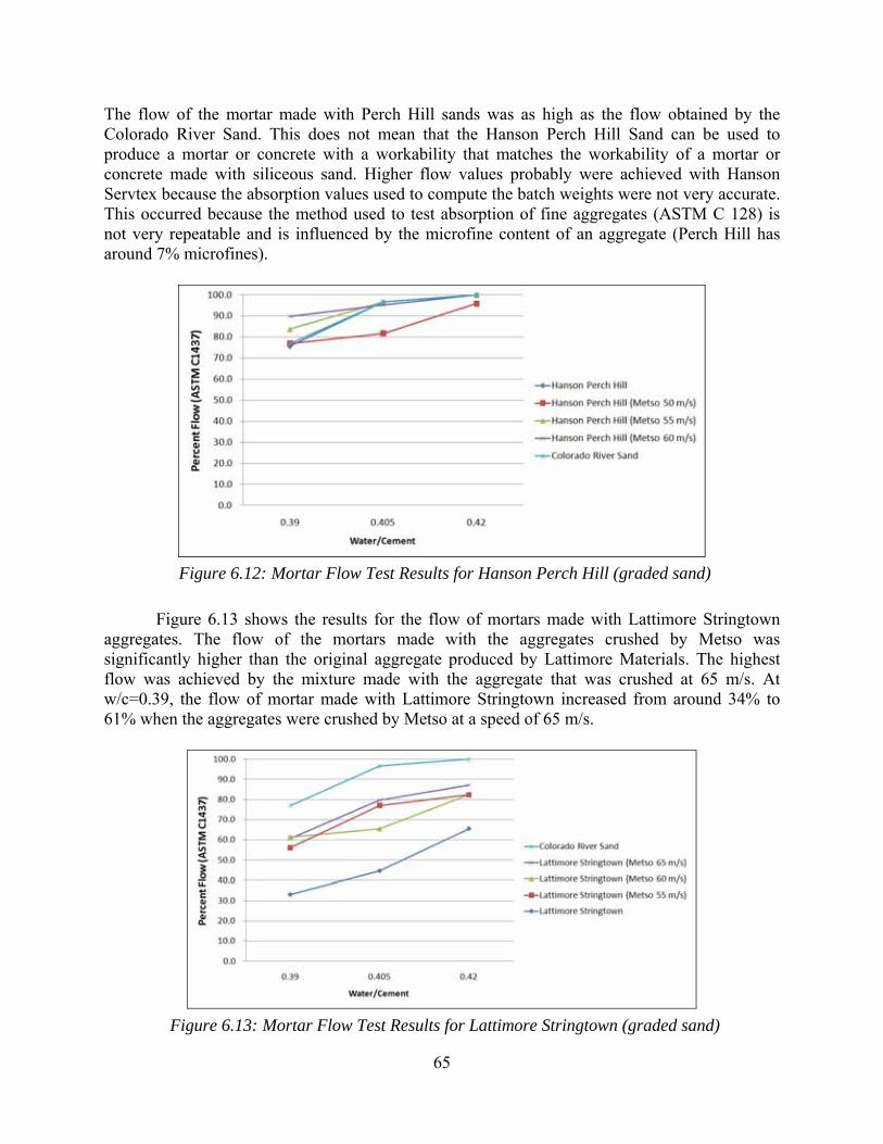
65

The flow of the mortar made with Perch Hill sands was as high as the flow obtained by the Colorado River Sand. This does not mean that the Hanson Perch Hill Sand can be used to produce a mortar or concrete with a workability that matches the workability of a mortar or concrete made with siliceous sand. Higher flow values probably were achieved with Hanson Servtex because the absorption values used to compute the batch weights were not very accurate. This occurred because the method used to test absorption of fine aggregates (ASTM C 128) is not very repeatable and is influenced by the microfine content of an aggregate (Perch Hill has around 7% microfines).

Figure 6.12: Mortar Flow Test Results for Hanson Perch Hill (graded sand)

Figure 6.13 shows the results for the flow of mortars made with Lattimore Stringtown aggregates. The flow of the mortars made with the aggregates crushed by Metso was significantly higher than the original aggregate produced by Lattimore Materials. The highest flow was achieved by the mixture made with the aggregate that was crushed at 65 m/s. At w/c=0.39, the flow of mortar made with Lattimore Stringtown increased from around 34% to 61% when the aggregates were crushed by Metso at a speed of 65 m/s.

Figure 6.13: Mortar Flow Test Results for Lattimore Stringtown (graded sand)

66

Conclusions 6.5

The testing described in this chapter evaluated the shape of aggregates obtained from different sources and crushed at varying speeds. Results from the three different testing methods used to evaluate the aggregate also permitted the evaluation of the test methods themselves.

MRTC was able to improve the shape of the Lattimore Stringtown aggregate using the Barmac B3000 VSI crusher. The improvement in shape was identified visually (Figure 6.3) and by testing the flow of a mortar made with the different Lattimore Stringtown aggregates (Figure 6.13). AIMS was not effective in evaluating the Lattimore Stringtown aggregates, mainly because AIMS is capable of evaluating only the 2D form and the angularity index of fine aggregates. Further, AIMS failed to measure the flatness of the Lattimore Stringtown aggregate (the flatness of this aggregate can be visually identified in Figure 6.3). AIMS is not capable of differentiating between flat and cubical aggregates because, as mentioned, it evaluates only the 2D form. Flat aggregates set on the AIMS tray will tend to lie on their flat side, meaning AIMS cannot measure the flatness of those aggregates because only the image on the non-flat side is recorded and evaluated.

The mortar flow test method described in this chapter was probably the best method used to indirectly evaluate the shape and texture of fine aggregate. The problem with the mortar flow test is that it is more time intensive (especially if graded sands are used). The results of the mortar flow test were also influenced by the accuracy of the measured absorption capacity of the aggregates being compared.

67

Proportioning PCC Containing MFAs Chapter 7.

One main issue encountered in using MFAs in PCC involves workability. The proportioning methods commonly used for siliceous sands do not work well for manufactured sands because MFAs have poor shape and grading (grading that does not meet ASMT C 33). This chapter describes work done to evaluate the proportioning method developed by ICAR. The only concrete property tested in this chapter was workability (slump). No hardened properties were evaluated because the hardened properties were tested using standard mixtures (Chapter 10). Optimizing mixtures by reducing cement content improves the durability of concrete without reducing strength [Fowler et al., 2008]; this is also why testing hardened property for optimized mixtures is not necessary. Suggested modifications to the ICAR method for proportioning pavement concrete are presented at the end of this chapter.

The ICAR Proportioning Method 7.1

Much of ICAR’s work involved finding better methods of proportioning MFA in concrete. The problem with using conventional methods for proportioning MFA in concrete is that those methods result in mixtures with higher cement content (or paste – water + cement). Higher cement content is not desirable because it adds to the cost of concrete and negatively affects the durability of the concrete (shrinkage, ASR, etc.). The proportioning method developed by Koehler and Fowler (2007) that was modified by McLeroy (2009) for pavement concrete was discussed in Section 3.4.2. This method could be summarized in the following five steps:

1. Evaluating aggregate properties.

2. Plotting the modified 0.45 power curve to determine the optimum gradation. This step involves choosing the percent of each coarse and fine aggregate needed to obtain the maximum aggregate density. The modified 0.45 power curve does not account for microfines (aggregates passing the No. 200 sieve).

3. Performing a combined dry-rodded unit weight (DRUW) test on the selected proportions of aggregates to determine the minimum paste requirements ( VoidspasteV − ).

4. Adding paste to achieve the desired workability ( spacingpasteV _ ). This paste value is based on

aggregate shape. This value is also dependent on the desired workability. McLeroy (2009) determined that an addition of 3 to 8 percent paste by volume was needed for pavement concrete made with MFA containing high microfine content. To compute this value, McLeroy (2009) used a visual shape and angularity rating (Figure 7.1).

_ = 3 + × ( − 1) (Eq. 7.1)

68

Figure 7.1: Visual Shape and Angularity Rating Scale McLeroy (2009)

5. Reducing the cement and water content based on the percentage of No. 200 fines present in the aggregates. In this step the percent microfines in the aggregates are subtracted from the paste content (paste = cementitious materials + water) while maintaining a constant water-to-cementitious ratio. Microfines are not accounted for as cementitious materials but as powder (powder = cementitious + microfines).

Preliminary Modifications to the ICAR Proportioning Method 7.2

Before any testing was done to evaluate the ICAR method, the fourth step which involved determining the additional paste needed based on the shape of the aggregates was modified. The modification was made because the visual shape and angularity rating used by McLeroy (2009) was subjective. Instead of using Figure 7.1, the 2D form and angularity indices determined using AIMS were used. As discussed in Chapter 6, AIMS evaluates the shape of fine aggregates by using a 2D form index. The lower the form index the more equidimensional a particle is. AIMS also evaluates the angularity of fine aggregates. The scale used ranges from 0 to 10,000; 0 indicates the presence of well round aggregates, and 10,000 indicates the presence of highly angular aggregates. Note that this work was done before the results of Chapter 6 were obtained. Those results showed that AIMS was not capable of properly evaluating flat fine aggregates.

In the third step of the ICAR method the minimum paste is computed using the dry-rodded unit weight. This minimum paste is the paste required to coat the aggregates. The additional paste, which is computed in the fourth step of the ICAR method, is the paste needed to achieve the desired workability. The percentage of that paste is related to its flow; the higher the flow, the less of that additional paste needed to achieve the required workability. For this reason, a flow test was run on four aggregates and the results were compared to the AIMS values to determine how flow and AIMS values relate. The tested aggregates included the Colorado River Sand, Hanson Servtex, Texas Crushed Stone, and Capital Marble Falls (those aggregates were not as flat as Lattimore Stringtown was). The aggregates were designated with numbers based on their shape: aggregate 1 was a natural sand with a good shape, Aggregate 2 was an MFA with a good shape, and Aggregates 3 and 4 were MFAs with relatively poor shape. For each of those

69

aggregates the cumulative percentage of aggregate with a shape ≤ 6 was computed (Table 7.1—highlighted in yellow). Aggregate 1 had the highest percentage (indicating a good shape factor); Aggregates 3 and 4 had the worse shape factor (lower cumulative percentages).

Cumulative 2D Form Index Table 7.1:

Aggregate 1(Cum. %)

Aggregate 2(Cum. %)

Aggregate 3(Cum. %)

Aggregate 4 (Cum. %)

≤ 6 42.7 29.8 17.8 14.7

≤ 12 96.6 95.1 93.5 93.8≤ 20 100 100 100 100

Table 7.2 shows the results of the cumulative angularity index for the four aggregates

used in this study. Aggregates 1 and 2 had higher percentage of particles with an angularity index ≤ 3300; therefore they were less angular than aggregates 3 and 4.

Cumulative Angularity Index Table 7.2:

Aggregate 1(Cum. %)

Aggregate 2(Cum. %)

Aggregate 3(Cum. %)

Aggregate 4 (Cum. %)

≤ 3300 79.1 68.2 50.4 55.6 ≤ 6600 99.7 99.2 98.5 100 ≤ 10000 100 100 100 100

Note that Aggregate 1 had the best shape and angularity index while aggregate 2 had a

shape and angularity index that was better than aggregates 3 and 4. Aggregate 3 had a better shape index than aggregate 4 but had a lower angularity index.

To evaluate whether or not those indices of shape and angularity could relate to concrete workability, the flow of mortars made with these aggregates was evaluated. ASTM C 1437 was used to measure the flow of mortar. To evaluate shape and angularity without including the effect of gradation, all fine aggregates were washed, sieved, and then re-graded to have the same gradation. All mortar mixtures had the same volume (1 liter) and were batched based on SSD values with no additions of admixtures. The same procedures described in section 6.3 were used. The results obtained are shown in Figures 7.2 and 7.3.

70

Figure 7.2: Flow of Aggregates with Different Shape and Angularity (5.5 sacks)

Figure 7.3: Flow of Aggregates with Different Shape and Angularity (6 sacks)

Results in Figure 7.2 represent a concrete mortar composed of a 5.5-sack mix, while Figure 7.3 represents a concrete mortar of a 6-sack mix. Comparing Figures 7.2 and 7.3 to results of Tables 7.1 and 7.2, shows that aggregates with higher 2D form and angularity index performed better than aggregates with lower indices. Thus shape and angularity values obtained from AIMS seemed to relate to concrete flow measured using ASTM C 1437.

The shape of aggregates measured by AIMS seemed to influence flow more than angularity did (comparing aggregate 3 and 4). Based on those results, the visual rating chart was

71

replaced by a linear AIMS function that increased the additional paste content in the mixture (up to 8%) as the AIMS form and angularity values increased. The function was made such that an increase in form would account for 80% of the increase in paste while the other 20% was associated to the angularity index. The goal was to start out with a basic AIMS function and to then to improve this function based on the slump results obtained from testing fine aggregates with various shapes. Note that the AIMS function was only used to evaluate fine aggregate shape since the shape of fine aggregates affect concrete workability more than the shape of coarse aggregates. The ICAR method also accounts for the shape of coarse aggregates indirectly through the combined dry-rodded unit weight test in step three.

Evaluating the ICAR Method 7.3

The ICAR method was evaluated using four different fine aggregates and one coarse aggregate; these included the Colorado River Sand, Capital Marble Falls (MFA), Hanson Servtex (MFA), Texas Crushed Stone (MFA), and a grade 4 coarse aggregate obtained from the Hanson Perch Hill quarry. All aggregate properties were first evaluated (Chapter 4) before the proportioning computations were performed (step one of section 7.1). One mixture was batched and tested for each mixture proportion considered in this chapter.

The second step of the ICAR method involves determining the optimum aggregate proportions using a modified 0.45 chart (discussed in Section 2.5.3); this was done for the four fine aggregates (Figures 7.4, 7.6, 7.8, and 7.9). The optimum grading using the modified 0.45 power chart was found to be at a sand-to-aggregate ratio of 0.3. This gradation was judged to be too coarse, so a different sand-to-aggregate ratio was also considered for two of the four fine aggregates. The second sand-to-aggregate ratio was determined using the conventional 0.45 power chart; the optimum gradation using such a curve corresponded to a sand-to-aggregate ratio of around 0.37 (Figures 7.5 and 7.7).

Figure 7.4: Capital Marble Falls S/A=0.30 (Modified 0.45 Power Chart)

72

Figure 7.5: Capital Marble Falls S/A=0.37 (Conventional 0.45 Power Chart)

Figure 7.6: Colorado River Sand S/A=0.30 (Modified 0.45 Power Chart)

73

Figure 7.7: Colorado River Sand S/A=0.37 (Conventional 0.45 Power Chart)

Figure 7.8: Texas Crushed Stone S/A=0.30 (Modified 0.45 Power Chart)

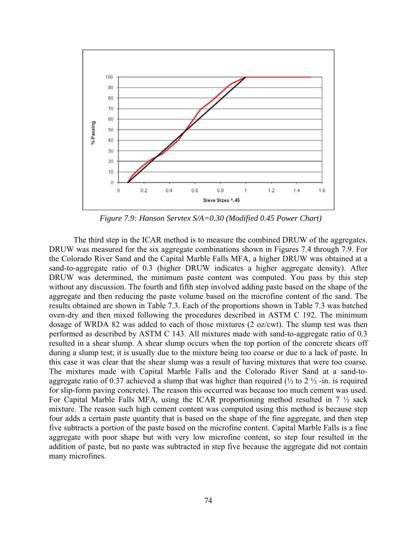
74

Figure 7.9: Hanson Servtex S/A=0.30 (Modified 0.45 Power Chart)

The third step in the ICAR method is to measure the combined DRUW of the aggregates. DRUW was measured for the six aggregate combinations shown in Figures 7.4 through 7.9. For the Colorado River Sand and the Capital Marble Falls MFA, a higher DRUW was obtained at a sand-to-aggregate ratio of 0.3 (higher DRUW indicates a higher aggregate density). After DRUW was determined, the minimum paste content was computed. You pass by this step without any discussion. The fourth and fifth step involved adding paste based on the shape of the aggregate and then reducing the paste volume based on the microfine content of the sand. The results obtained are shown in Table 7.3. Each of the proportions shown in Table 7.3 was batched oven-dry and then mixed following the procedures described in ASTM C 192. The minimum dosage of WRDA 82 was added to each of those mixtures (2 oz/cwt). The slump test was then performed as described by ASTM C 143. All mixtures made with sand-to-aggregate ratio of 0.3 resulted in a shear slump. A shear slump occurs when the top portion of the concrete shears off during a slump test; it is usually due to the mixture being too coarse or due to a lack of paste. In this case it was clear that the shear slump was a result of having mixtures that were too coarse. The mixtures made with Capital Marble Falls and the Colorado River Sand at a sand-to-aggregate ratio of 0.37 achieved a slump that was higher than required (½ to 2 ½ -in. is required for slip-form paving concrete). The reason this occurred was because too much cement was used. For Capital Marble Falls MFA, using the ICAR proportioning method resulted in 7 ½ sack mixture. The reason such high cement content was computed using this method is because step four adds a certain paste quantity that is based on the shape of the fine aggregate, and then step five subtracts a portion of the paste based on the microfine content. Capital Marble Falls is a fine aggregate with poor shape but with very low microfine content, so step four resulted in the addition of paste, but no paste was subtracted in step five because the aggregate did not contain many microfines.

75

Summary of the Results Obtained Using the ICAR Proportioning Method Table 7.3:

Capital Marble Falls (MFA) Colorado River Sand (Natural)

Texas Crushed Stone (MFA)

Hanson Servtex (MFA)

Sand/Aggregate 0.37 0.30 0.37 0.30 0.30 0.30W/C 0.45 0.45 0.45 0.45 0.45 0.45

Coarse Aggregates (lb/yd3) 1861.8 2107.3 2006.6 2274.2 2274.7 2214.0Fine Aggregates (lb/yd3) 1138.5 940.6 1147.6 949.1 938.6 913.3

Water (lb/yd3) 319.1 307.0 268.65 254.6 254.5 273.5 Cement (lb/yd3) 709.2 682.2 597.01 565.9 565.6 607.9

Sacks of Cement (lb/yd3) 7.54 7.26 6.35 6.02 6.02 6.47Slump (in.) 7- ¾ Shear Slump 3- ¾ Shear Slump Shear Slump Shear Slump

76

Determining the Optimum Paste Content for Pavement Concrete 7.4

The ICAR method developed by McLeroy (2009) worked for MFA containing high microfines but it did not work well with MFA not containing high microfine content. The problem encountered occurred after the minimum paste content was computed in step three. For this reason, a series of tests was made to determine the minimum paste addition needed to achieve the desired workability. Examples are shown in Tables 7.4 and 7.5.

Tables 7.4 and 7.5 show that the slump requirement was reached by just using the minimum paste volume computed using DRUW. In Table 6.2, a slump of 4 in. was obtained for the mixture containing no additional paste; a lower slump could be obtained if a lower dosage of admixture was used. The minimum paste content determined for the mixtures containing Capital Marble Falls corresponded to a 6.2-sack mixture. To obtain mixtures with lower cement content, a better gradation of coarse aggregate with a larger maximum size aggregate is needed. The coarse aggregate used for this testing was a grade 4; pavement mixtures are usually made with a grade 3 coarse aggregate or a combination of a grade 2 and grade 4. Compared to grade 4, both grades 2 and 3 have larger maximum size aggregates.

Determining the Optimum Paste Content for a Mixture Containing Capital Table 7.4:Marble Falls and a w/c=0.45

Sacks of Cement

Paste Added

Cement (lb/yd3)

Water (lb/yd3)

Fine Aggregate

(lb/yd3)

Coarse Aggregate

(lb/yd3)

Slump (in.)

WRDA Dosage

(oz/cwt) 6.2 0 581.9 261.9 1238.9 2026.1 4.0 9.4 6.4 1 603.9 271.7 1221.6 1997.7 2.0 6.0 6.7 2 625.8 281.6 1204.3 1969.4 3- ½ 5.36.9 3 647.8 291.5 1187.0 1941.1 7.1 4 669.7 301.4 1169.6 1912.7 7- ½ 5.5

Determining the Optimum Paste Content for a Mixture Containing Capital Table 7.5:Marble Falls and a w/c=0.42

Sacks of Cement

Paste Added

Cement (lb/yd3)

Water (lb/yd3)

Fine Aggregate

(lb/yd3)

Coarse Aggregate

(lb/yd3)

Slump (in.)

WRDA Dosage

(oz/cwt)

6.4 0 605.6 254.4 1238.9 2026.1 1- ¼ 7.8 6.7 1 628.4 263.9 1221.6 1997.7 1- ¾ 6.7 6.9 2 651.3 273.5 1204.3 1969.4 5.0 7.0 7.2 3 674.1 283.1 1187.0 1941.1 2.0 5.4

The same procedure shown in Figures 7.4 and 7.5 was applied for five other sands at a

water-to-cement ratio of 0.45 and a sand-to-aggregate ratio of 0.37. A summary of the results showing the percentage of additional paste required to achieve ½ to 2 ½ -in. of slump is shown in Table 7.6. More paste was needed for the mixture made with Texas Crushed Stone because that

77

MFA contained about 21% microfines. Lattimore Stringtown required less paste than the computed minimum paste requirement. This occurred because the combined DRUW measured for Lattimore Stringtown was relatively low. A low DRUW resulted in a high computed minimum paste content. Lattimore Stringtown has a low packing density when measured using DRUW; after mixing it in concrete, its packing density seemed to improve. Similar testing was also performed using TXI Bridgeport coarse aggregate. The results on quantity of paste that needed to be added to achieve required workability resembled the results shown in Table 7.6.

Additional Paste Required to Reach Target Workability Table 7.6:

Fine Aggregate Source Additional Paste Needed to Reach Target Slump (%)

Colorado River Sand 0Capital Marble Falls 0Texas Crushed Stone 2

TXI Bridgeport 0Hanson Perch Hill 0

Lattimore Stringtown -3

Recommendations 7.5

The ICAR proportioning method proposed by McLeroy (2009) for pavement concrete overestimates the amount of cement needed for mixtures containing MFA with low microfine content. To avoid overestimating the cement content, we recommend computing only the minimum paste content and not adding any additional paste before trial batches are evaluated (steps one to three of Section 7.1). Since pavement concrete is a low slump concrete, the minimum paste computed using DRUW should be enough to achieve ½ to 2 ½-in. slump (unless the MFA contains high microfines). However, if the slump is too low, the slump can be adjusted by making the paste more flowable; this can be achieved by adding a higher dosage of admixture.

The modified 0.45 power curve seemed to result in denser aggregate gradations, but it also resulted in aggregate proportions that caused shear slumps for the fine aggregates tested. The modified 0.45 power curve was developed by Fowler and Koehler (2007) for self-consolidating concrete (SCC), but the conventional 0.45 curve seemed to work better for proportioning pavement concrete. The ICAR method for pavement concrete could be summarized in the following five steps:

1. Evaluate aggregate properties (sieve analysis, specific gravity, and absorption).

2. Plot the 0.45 power chart to determine the optimum gradation of fine and coarse aggregate (Figure 7.10).

78

Figure 7.10: Example of a 0.45 Power Chart

3. Perform a combined DRUW test on the selected proportions of aggregates to determine the minimum paste volume (Figure 7.11).

Figure 7.11: Example of a Combined DRUW Test

4. Choose paste quality: w/c, percent air, SCM, admixture, etc.

5. Perform trial batches and adjust mixture proportions accordingly. If the workability could not be achieved and paste can be added to the mixture, then do so. On the other hand, if the trial batch shows that paste could be further reduced, then reduce the paste content.

Conclusions 7.6

Following are the advantages of using the ICAR proportioning method for pavement concrete:

• The method was specifically made for slipform concrete.

79

• The aggregate gradation is entirely based on power 0.45 chart. Other methods employ only the power 0.45 chart to proportion coarse aggregate and rely on the fineness modulus to determine the sand-to-aggregate ratio.

• This method could be used for any aggregate regardless of individual aggregate gradation.

• Unlike other proportioning methods, this method accounts for aggregate shape indirectly through the combined DRUW.

• It is a simple method to reach optimized proportions for a combination of aggregates.

• Only basic equipment is needed to perform all the testing required for design.

80

81

Preliminary Skid Testing Chapter 8.

Most of ICAR’s work involved finding better proportioning methods for MFA and testing hardened properties of concrete made with MFA, including strength, modulus of elasticity, abrasion resistance, and coefficient of thermal expansion. However, none of the ICAR projects evaluated skid resistance of concrete. When this research project started in fall 2008, it was not clear what methods were going to be used to measure skid resistance in the laboratory. TxDOT suggested using the CTM (discussed in Section 3.3.1) and the DFT (discussed in Section 3.3.2) to evaluate skid resistance of concrete in the laboratory and in the field. Those two devices had previously been used on a similar TxDOT project that involved evaluating skid resistance of asphalt pavements. The CTM and DFT are shown in Figures 8.1 and 8.2.

Figure 8.1: Circular Track Meter

Figure 8.2: Dynamic Friction Tester

Most of the literature found on the usage of those devices was from research on asphalt concrete. Therefore, preliminary testing was conducted to evaluate the two devices. The goal of the preliminary testing described in this chapter was to

1. Better understand how the texture and friction values obtained from the CTM and DFT relate to concrete textures.

2. Establish a testing protocol for evaluating the polish resistance of concrete.

82

Evaluating the Texture of Concrete Made by Different Finishing 8.1Techniques

Five surfaces with different textures were evaluated using the CTM and DFT. Four of those were 24-in. by 24-in. concrete slabs that were cast in the laboratory. The same mixture was used to cast all four concrete surfaces. Following are the five surfaces evaluated:

1. A broom finish (Figure 8.3)

2. Burlap drag finish (Figure 8.4)

3. Tined and burlap drag finish (Figure 8.5)

4. A trowel finish (Figure 8.6); a steel trowel was used to obtain a smooth surface.

5. Smooth glass surface (Figure 8.7). This surface was evaluated to measure how low of a friction and texture value could be obtained using those devices. Since the CTM is a laser-based device, the surface of the glass was painted after friction measurements using the DFT were taken.

Figure 8.3: Broom Finish Figure 8.4: Burlap Drag

Figure 8.5: Tined + Burlap Drag Figure 8.6: Trowel Finish

83

Figure 8.7: Painted Glass

The CTM was used to measure texture on three different locations on each of the surfaces. The profiles obtained for the different surfaces using the CTM are shown in Figure 8.8. The CTM measures the Mean Profile Depth (MPD); the MPD is a measure of the macro-texture of a surface. The range of the MPD values for the five surfaces is shown in Figure 8.9. The highest MPD was obtained by using a broom finish. Tining a surface significantly increased the MPD values measured. The MPD value of a surface finished with a burlap drag almost doubled after the surface was tined. The surface that was trowel finished had the lowest MPD value among the four concrete specimens. The glass surface had very low MPD values; the values were higher than zero because the surface was painted.

Figure 8.8: Texture Profiles

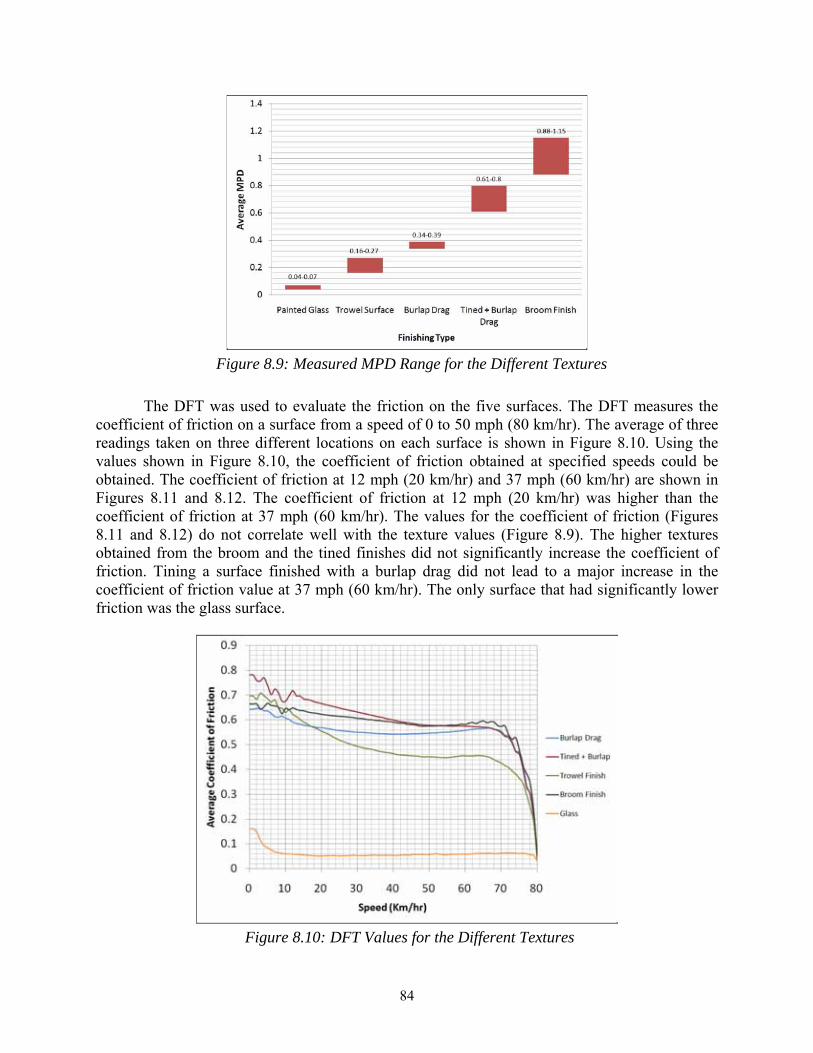
84

Figure 8.9: Measured MPD Range for the Different Textures

The DFT was used to evaluate the friction on the five surfaces. The DFT measures the coefficient of friction on a surface from a speed of 0 to 50 mph (80 km/hr). The average of three readings taken on three different locations on each surface is shown in Figure 8.10. Using the values shown in Figure 8.10, the coefficient of friction obtained at specified speeds could be obtained. The coefficient of friction at 12 mph (20 km/hr) and 37 mph (60 km/hr) are shown in Figures 8.11 and 8.12. The coefficient of friction at 12 mph (20 km/hr) was higher than the coefficient of friction at 37 mph (60 km/hr). The values for the coefficient of friction (Figures 8.11 and 8.12) do not correlate well with the texture values (Figure 8.9). The higher textures obtained from the broom and the tined finishes did not significantly increase the coefficient of friction. Tining a surface finished with a burlap drag did not lead to a major increase in the coefficient of friction value at 37 mph (60 km/hr). The only surface that had significantly lower friction was the glass surface.

Figure 8.10: DFT Values for the Different Textures

85

Figure 8.11: DFT20 Values for Different Textures

Figure 8.12: DFT60 Values for Different Textures

Results show that the CTM can differentiate between the different types of finishing techniques. The CTM is a device that is good for evaluating macro-texture; macro-texture in PCC is intentionally formed to provide skid resistance and to drain water from concrete pavements. Macro-texture formed on concrete is not expected to contribute to long-term skid resistance (reviewed in 2.1.5 and 3.2.3.2). The DFT cannot differentiate between the types of finishings created on the surface of the concrete because the DFT evaluates friction; having higher macro-texture does not seem to always lead to higher friction values and that is why no clear correlation exists between the MPD values and friction values. For example, the surface finished using a trowel had a low MPD value compared to the tined surface (Figure 8.9), but the

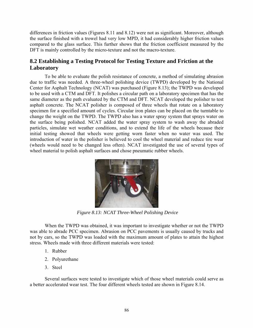
86

differences in friction values (Figures 8.11 and 8.12) were not as significant. Moreover, although the surface finished with a trowel had very low MPD, it had considerably higher friction values compared to the glass surface. This further shows that the friction coefficient measured by the DFT is mainly controlled by the micro-texture and not the macro-texture.

Establishing a Testing Protocol for Testing Texture and Friction at the 8.2Laboratory

To be able to evaluate the polish resistance of concrete, a method of simulating abrasion due to traffic was needed. A three-wheel polishing device (TWPD) developed by the National Center for Asphalt Technology (NCAT) was purchased (Figure 8.13); the TWPD was developed to be used with a CTM and DFT. It polishes a circular path on a laboratory specimen that has the same diameter as the path evaluated by the CTM and DFT. NCAT developed the polisher to test asphalt concrete. The NCAT polisher is composed of three wheels that rotate on a laboratory specimen for a specified amount of cycles. Circular iron plates can be placed on the turntable to change the weight on the TWPD. The TWPD also has a water spray system that sprays water on the surface being polished. NCAT added the water spray system to wash away the abraded particles, simulate wet weather conditions, and to extend the life of the wheels because their initial testing showed that wheels were getting worn faster when no water was used. The introduction of water in the polisher is believed to cool the wheel material and reduce tire wear (wheels would need to be changed less often). NCAT investigated the use of several types of wheel material to polish asphalt surfaces and chose pneumatic rubber wheels.

Figure 8.13: NCAT Three-Wheel Polishing Device

When the TWPD was obtained, it was important to investigate whether or not the TWPD was able to abrade PCC specimen. Abrasion on PCC pavements is usually caused by trucks and not by cars, so the TWPD was loaded with the maximum amount of plates to attain the highest stress. Wheels made with three different materials were tested:

1. Rubber

2. Polyurethane

3. Steel

Several surfaces were tested to investigate which of those wheel materials could serve as a better accelerated wear test. The four different wheels tested are shown in Figure 8.14.

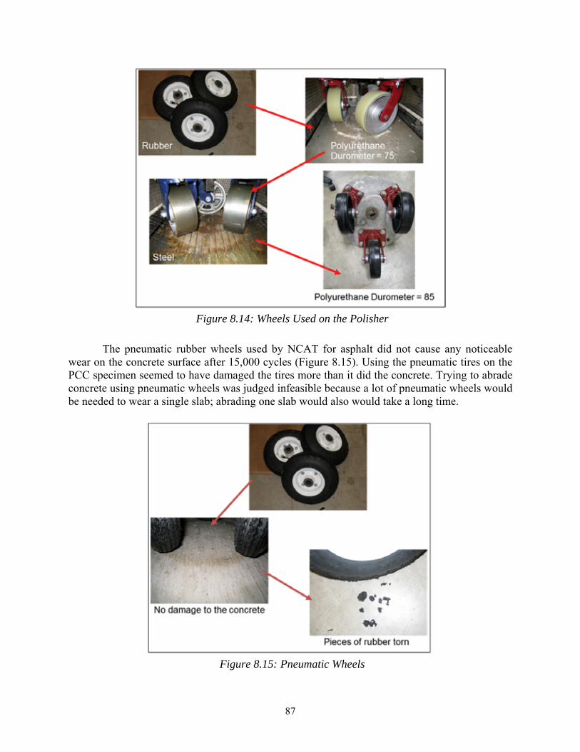
87

Figure 8.14: Wheels Used on the Polisher

The pneumatic rubber wheels used by NCAT for asphalt did not cause any noticeable wear on the concrete surface after 15,000 cycles (Figure 8.15). Using the pneumatic tires on the PCC specimen seemed to have damaged the tires more than it did the concrete. Trying to abrade concrete using pneumatic wheels was judged infeasible because a lot of pneumatic wheels would be needed to wear a single slab; abrading one slab would also would take a long time.

Figure 8.15: Pneumatic Wheels

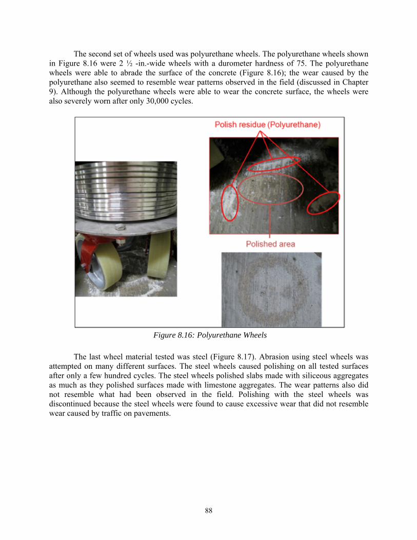
88

The second set of wheels used was polyurethane wheels. The polyurethane wheels shown in Figure 8.16 were 2 ½ -in.-wide wheels with a durometer hardness of 75. The polyurethane wheels were able to abrade the surface of the concrete (Figure 8.16); the wear caused by the polyurethane also seemed to resemble wear patterns observed in the field (discussed in Chapter 9). Although the polyurethane wheels were able to wear the concrete surface, the wheels were also severely worn after only 30,000 cycles.

Figure 8.16: Polyurethane Wheels

The last wheel material tested was steel (Figure 8.17). Abrasion using steel wheels was attempted on many different surfaces. The steel wheels caused polishing on all tested surfaces after only a few hundred cycles. The steel wheels polished slabs made with siliceous aggregates as much as they polished surfaces made with limestone aggregates. The wear patterns also did not resemble what had been observed in the field. Polishing with the steel wheels was discontinued because the steel wheels were found to cause excessive wear that did not resemble wear caused by traffic on pavements.

89

Figure 8.17: Steel Wheels

The best results were obtained using the polyurethane wheels. For this reason a second set of polyurethane wheels was obtained. The black polyurethane wheels (Figure 8.14) were 2-in. wide and had a durometer hardness of 85. Four mortar slabs were abraded using those polyurethane wheels; two were made with siliceous sand (Colorado River Sand), and the other two were made with a limestone MFA (Texas crushed stone). For those slabs friction and texture measurements were taken before the slabs were abraded and after each abrasion cycle using the CTM and DFT. The change in texture measured using the CTM are shown in Figure 8.18. Compared to the slabs made with limestone, the slabs made with siliceous sand had lower MPD values before and after abrading the surface.

90

Figure 8.18: Change in Texture Values for the River Sand and Limestone MFA

The change in friction values measured by the DFT is shown in Figure 8.19. Although the slabs made with the limestone sand had higher texture (Figure 8.18), the slabs made with siliceous sand had higher friction values. The friction values for the slabs made with siliceous sand remained to be higher than the slabs made with limestone MFA even after 60,000 polishing cycles.

Figure 8.20 shows a picture of a slab made with siliceous sand. The TWPD abraded the wheel path and exposed the siliceous fine aggregates. The exposed fine aggregates were not polished after 60,000 cycles, and the unpolished fine aggregates provided the skid resistance. Figure 8.21 shows a picture of an abraded slab made with limestone MFA. Although the slab seems to still have considerable macro-texture, the top portion of the macro-texture polished; this was what caused the loss in friction.

Figure 8.19: Change in Friction Values for the River Sand and Limestone MFA

91

Figure 8.20: Slab Made with Siliceous Sand

Figure 8.21: Slab Made with Limestone MFA

92

The difference in wear patterns between concrete made with hard and soft fine aggregates is shown in Figure 8.22. Abrasion caused by traffic exposes fine aggregates; harder fine aggregates do not polish and provide frictional resistance, while soft fine aggregates that are exposed polish and cause a drop in frictional resistance.

Figure 8.22: Surface Made with Siliceous Sand vs. Limestone MFA

Conclusions 8.3

The preliminary testing described in this chapter was necessary to learn how to use the CTM, DFT, and TWPD to evaluate concrete surfaces for skid resistance at the laboratory and in the field. The results obtained from the DFT correlated better with the expected performance of sands. The DFT values did not correlate well with the texture values obtained using the CTM. The macro-texture measured by the CTM is not a good measure of friction; higher MPD values did not always correlate with higher friction values measured by the DFT. The comparison between the trowel-finished surface and the glass surface shows that even concrete surfaces with low macro-texture could still have significant friction. This also showed that the DFT is a better tool for evaluating polished surfaces (the glass surface represents a very polished surface). The materials and setting on the TWPD needed to polish PCC specimen were also investigated. The wheels adopted for the concrete test were polyurethane; the pneumatic wheels used by NCAT for polishing asphalt specimen did not sufficiently abrade the concrete surface like they did on asphalt concrete.

93

Field Testing for Skid Resistance Chapter 9.

Twelve field sections in five different locations were evaluated for skid resistance using a CTM and DFT. Some of those sections were chosen because they were the only known sections made with materials that did not meet the AI requirements. The first location had four sections, three of which were constructed with 100% limestone MFA, while the fourth section was a control section made with blended sands. The second location contained three sections made from three different blends of siliceous sand and limestone MFA. The other three locations had sections that were made with fine aggregates that met the AI requirements—those sections were evaluated to obtain a wider range of skid numbers, which were needed to get better correlation between CTM, DFT, and skid trailer values.

Test Equipment Correlation 9.1

CTM, DFT, and skid trailer measurements were taken on twelve different PCC pavements sections to evaluate the correlation between different testing equipment (all twelve sections had a carpet drag and tined finish surface). Three to four CTM and DFT measurements were taken in the wheel path of each of the test sections; measurements were taken 50 to 200 feet apart, depending on how long each section was. A skid trailer equipped with smooth tires was then used to skid the same sections at 50 mph. Using equations presented in Chapter 3 (Equations 3.1, 3.2, and 3.3), the average equivalent skid numbers for each section was computed. Figure 9.1 shows a comparison between computed skid values and the actual skid values measured using a skid trailer.

Figure 9.1: Computed vs. Measured SN(50)smooth

Results from Figure 9.1 indicate that the IFI formula was not able to predict the measured skid number. Figures 9.2 and 9.3 show that better correlation was obtained when the measured skid trailer values were compared to friction values at 12 and 37 mph (20 and 60 km/hr) (DFT20 and DFT60).

94

Figure 9.2: DFT20 vs. Measured SN(50)smooth

Figure 9.3: DFT60 vs. Measured SN(50)smooth

Figure 9.4 shows that there is no correlation between SN(50)smooth and the MPD measured by the CTM. The poor correlation between SN(50)smooth and MPD, which is used to compute the IFI parameters, explains the poor correlation between the measured and IFI computed SN(50)smooth.

95

Figure 9.4: MPD vs. Measured SN(50)smooth

Based on the results obtained in Figures 9.1, 9.2, 9.3, and 9.4, the best method to compute SN(50)smooth using laboratory equipment is by using the following equation: (50) = .. (Eq. 9.1)

where DFT60 is the average coefficient of friction at 37 mph (60 km/hr) measured using the DFT at different locations along a concrete section.

Note that Equation 9.1 was established for concrete surfaces that have a mortar finish. It is not known whether or not Equation 9.1 accurately predicts SN(50)smooth for other types of finishing such as diamond ground or exposed aggregate.

Sections Made with 100% MFA 9.2

Construction of the 100% MFA Sections 9.2.1

The 100% MFA sections were constructed in 2008 as part of a TxDOT implementation project on the usage of MFA containing high microfine content in PCC pavements. The three sections were made with the same source of limestone sand but with varying microfine contents. Information provided in this chapter about the construction of those three test sections was obtained from the report written by McLeroy (2009).

In the manufactured aggregate production process, after rock pieces are conveyed to a crusher, the resulting product is sieved over a No. 4 screen into coarse and fine aggregate. The fine aggregate which is known as the dry screenings is then conveyed to a wet sieving operation. This is done to reduce the fines passing the No. 200 sieve. The wet-sieved product is known as the manufactured sand.

Since the aim of that implementation project was to use sands with varying percentages of microfines, the two types of sands, dry screening and manufactured sand, were combined in different amounts to create fine aggregate blends with 5, 10, and 15% microfine content [McLeroy, 2008]. The gradation of the manufactured sand and the dry screenings are shown in Table 9.1.

96

Fine Aggregate Grading [McLeroy, 2008] Table 9.1:

% Retained

US Sieve Manufactured Sand Dry Screenings

#4 2 2.9

#8 28.1 19.0

#16 29.2 22.4

#30 17.8 16.4

#50 10.5 13.6

#100 5 6.2

#200 1.9 4

Pan 5.5 15.4

The two limestone coarse aggregates used in this implementation project were obtained

from the same source as the fine aggregates. The difference between the two aggregates was in their grading; the first was a TxDOT Grade 2 (1 ½-in. maximum size aggregate) and the other aggregate was a TxDOT Grade 4 (1-in. maximum size aggregate). The reason two different coarse aggregates were combined was to obtain better packing of aggregates. Combining a Grade 2 and Grade 4 coarse aggregate is common to the optimized concrete mixtures used in the Fort Worth district. Other materials used on this project included a Type I/II cement (ASTM C 150), a Class C fly ash (ASTM C 618), an air entraining admixture (ASTM C 260), and a water-reducing and retarding admixture (ASTM C 494 Type D) [McLeroy, 2008].

The optimized mixture used for this project is a mixture typically used on TxDOT projects for Class P concrete made with blended sands (Class P is pavement concrete). To create mixtures with microfine contents of 5%, 10%, and 15%, three different blends of sands were used. Table 9.2 shows the batch quantities for each of the three mixtures.

Concrete Mixture Proportions [McLeroy, 2008] Table 9.2:

Concrete Mixtures Proportions (lb/yd3)

5% 10% 15% Cement 362 362 362Fly Ash 155 155 155Water 233 233 233

Coarse Aggregate - Grade 2 636 636 636Coarse Aggregate - Grade 4 1,177 1,177 1,177

Drying Screenings (TXI Bridgeport) 0 684 1,368Manufactured Sands (TXI Bridgeport) 1,368 684 0

Laboratory testing for fresh and hardened properties was conducted on each of the three

mixtures prior to field implementation [McLeroy, 2008]; these properties included slump (Tex-430-A), unit weight (ASTM C 138), compressive strength (Tex-418-A), modulus of elasticity, abrasion resistance (ASTM C 944), and coefficient of thermal expansion (Tex-428-A). A

97

summary of all the results is shown in Table 9.3. The goal of those tests was to ensure that the performance of the concrete made with limestone MFA can meet TxDOT requirements. The abrasion test was included to show that the addition of microfines does not necessarily reduce abrasion resistance (as implied by ASTM C 33). All properties tested for those three mixtures yielded acceptable results. It should be noted, however, that the concrete was evaluated for abrasion resistance and not for skid resistance. ASTM C 944 is a test that evaluates wear of concrete or mortar by measuring the loss in mass and not the loss in texture or friction. The abrasion/wear test described in ASTM C 944 better relates to wear caused by the use of studded tires rather than polish caused by traffic.

Laboratory Concrete Tests Results Obtained from McLeroy (2008) Table 9.3:

Concrete Mixtures

5% 10% 15% Slump (in.) 0.5 2.75 0.75

Unit Weight (lb/ft3) 150 148 151 28-day Compressive

Strength (psi) 6,370 6,155 6,160

28-day Modulus of Elasticity (ksi) 5,320 5,310 5,360

Coefficient of Thermal Expansion (µstrain/°C) 5.1 5.1 4.9

Abrasion (average loss - grams) 0.9 1.3 1.1

The next part of this project was to implement the mixtures tested at the laboratory and in

the field. Paving began on the 5% microfine mixture in July 2008. The first truck delivered to the site had a concrete temperature between 90-95°F (32-35°C) [McLeroy, 2008]. The first truck was rejected, but the high temperatures remained a problem in subsequent trucks [McLeroy, 2008]. The slump measured for the concrete shown in Figure 9.5 was around ¼ -in. which is below the TxDOT requirements of ½ to 2 ½ -in. slump. The paving machine did not have much effect vibrating the low slump concrete that was being delivered. Some of the concrete delivered also had higher workability than what was required (Figure 9.6). This was probably due to the addition of water to the concrete.

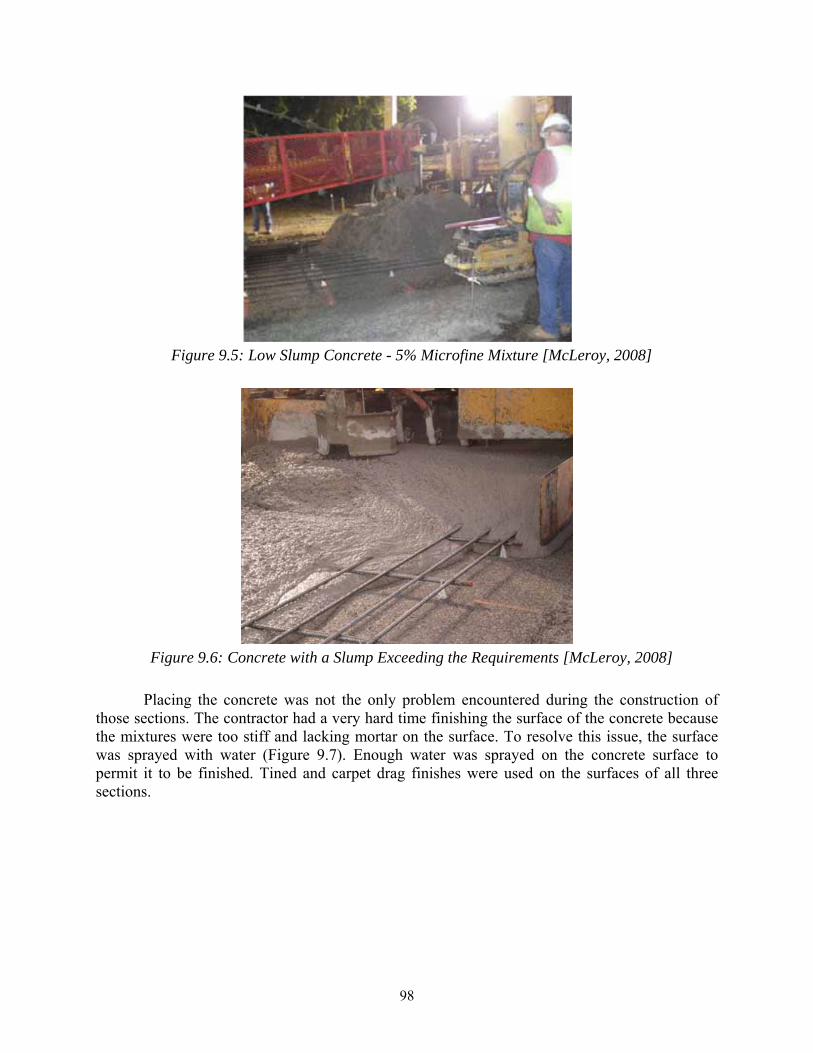
98

Figure 9.5: Low Slump Concrete - 5% Microfine Mixture [McLeroy, 2008]

Figure 9.6: Concrete with a Slump Exceeding the Requirements [McLeroy, 2008]

Placing the concrete was not the only problem encountered during the construction of those sections. The contractor had a very hard time finishing the surface of the concrete because the mixtures were too stiff and lacking mortar on the surface. To resolve this issue, the surface was sprayed with water (Figure 9.7). Enough water was sprayed on the concrete surface to permit it to be finished. Tined and carpet drag finishes were used on the surfaces of all three sections.

99

Figure 9.7: Finishability Problems Encountered with 100% MFA Sections [McLeroy, 2008]

A fourth section was constructed adjacent to the three sections made with 100% MFA and referred to as the TxDOT optimized mixture. This section was a control section that had 50% siliceous and 50% limestone MFA (Table 9.4). No workability or finishability problems were encountered when this section was cast.

TxDOT Optimized Mixture Design Table 9.4:

Concrete Mixtures Proportions (lb/yd3)

TxDOT Optimized Cement 394Fly Ash 170Water 254

Coarse Aggregate - Grade 2 620Coarse Aggregate - Grade 4 1148

Manufactured Sands (TXI Bridgeport) 667 Siliceous Sand (TXI Paradise) 664

Table 9.5 shows the difference between the compressive strength of the concrete made at

the laboratory and that of the concrete used for the field sections. The concrete used in the field

100

probably had higher water-to-cement ratio (and that is not even accounting for the surface of the concrete).

Lab and Field Compressive Strength Table 9.5:

Concrete Mixtures 5% 10% 15%

28-day Compressive Strength - Lab (psi) 6,370 6,155 6,160

28-day Compressive Strength - Field (psi) 5,480 5,240 4,850

Standard Deviation of Field Compressive Strength (psi) 720 230 330

Texture and Friction Evaluation of 100% MFA Sections 9.2.2

Four visits have been made since the sections were constructed in 2008. During those two visits, the texture and friction of the sections were measured using the CTM and DFT. Figure 9.8 shows that sections 1 and 2 seem to be highly polished on the wheel path. Section 3 and 4 were constructed on the inside lane—thus both those sections were exposed to different traffic. The outside lane (sections 1 and 2) is exposed to more truck traffic, and that is probably why sections 1 and 2 were more polished than section 3.

Figure 9.8: 100% MFA Sections December 2010

The 100% MFA sections were monitored for three years. CTM and DFT measurements were taken during four visits to the site and the values were converted using Equation 9.1. Measurements taken between the wheel paths are generally not exposed to traffic and were assumed to represent the initial conditions of the pavement (June, 2008). The data obtained are shown in Figure 9.9.

101

Figure 9.9: Computed Skid Numbers for Trial Field Sections as a Function of Time

Figure 9.9 shows that a change in microfine content (gradation change) did not have any effect on skid resistance. Even though section 2 had slightly higher initial skid values, sections 1 and 2 had very similar skid values after more than 1 year of traffic. Results obtained from Figure 9.9 also show that trucks have a higher wearing and polishing effect on pavements. The inside lane and the outside lane might have the same average daily traffic (ADT) count but they almost assuredly have different 18-kip Equivalent Single Axle load (ESAL) counts.

Figures 9.10, 9.11, 9.12, and 9.13 show the difference between the pavement surfaces on the wheel paths and between the wheel paths. Sections 1 and 2 were clearly more abraded and polished than sections 3 and 4 on the wheel path (high loss of macro-texture). The between-the-wheel-path pictures show that all sections had the same finishing.

Figure 9.10: Section 1 Wheel Path (left) vs. Between Wheel Path (right)

102

Figure 9.11: Section 2 Wheel Path (left) vs. Between Wheel Path (right)

Figure 9.12: Section 3 Wheel Path (left) vs. Between Wheel Path (right)

Figure 9.13: Section 4 Wheel Path (left) vs. Between Wheel Path (right)

Blended Sand Sections 9.3

In 1995, three sections were constructed by TxDOT with blends of sands not meeting the TxDOT 60% AI limit. The three sections were constructed on the inside lane of a highway mainly used by trucks transporting aggregates (the sections are subject to a very high percentage of truck traffic). The following blends of fine aggregates were used for those three sections:

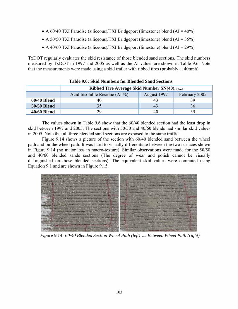
103

• A 60/40 TXI Paradise (siliceous)/TXI Bridgeport (limestone) blend (AI = 40%)

• A 50/50 TXI Paradise (siliceous)/TXI Bridgeport (limestone) blend (AI = 35%)

• A 40/60 TXI Paradise (siliceous)/TXI Bridgeport (limestone) blend (AI = 29%) TxDOT regularly evaluates the skid resistance of those blended sand sections. The skid numbers measured by TxDOT in 1997 and 2005 as well as the AI values are shown in Table 9.6. Note that the measurements were made using a skid trailer with ribbed tires (probably at 40mph).

Skid Numbers for Blended Sand Sections Table 9.6:

Ribbed Tire Average Skid Number SN(40)ribbed Acid Insoluble Residue (AI %) August 1997 February 2005

60/40 Blend 40 43 39 50/50 Blend 35 43 36 40/60 Blend 29 40 35

The values shown in Table 9.6 show that the 60/40 blended section had the least drop in

skid between 1997 and 2005. The sections with 50/50 and 40/60 blends had similar skid values in 2005. Note that all three blended sand sections are exposed to the same traffic.

Figure 9.14 shows a picture of the section with 60/40 blended sand between the wheel path and on the wheel path. It was hard to visually differentiate between the two surfaces shown in Figure 9.14 (no major loss in macro-texture). Similar observations were made for the 50/50 and 40/60 blended sands sections (The degree of wear and polish cannot be visually distinguished on those blended sections). The equivalent skid values were computed using Equation 9.1 and are shown in Figure 9.15.

Figure 9.14: 60/40 Blended Section Wheel Path (left) vs. Between Wheel Path (right)

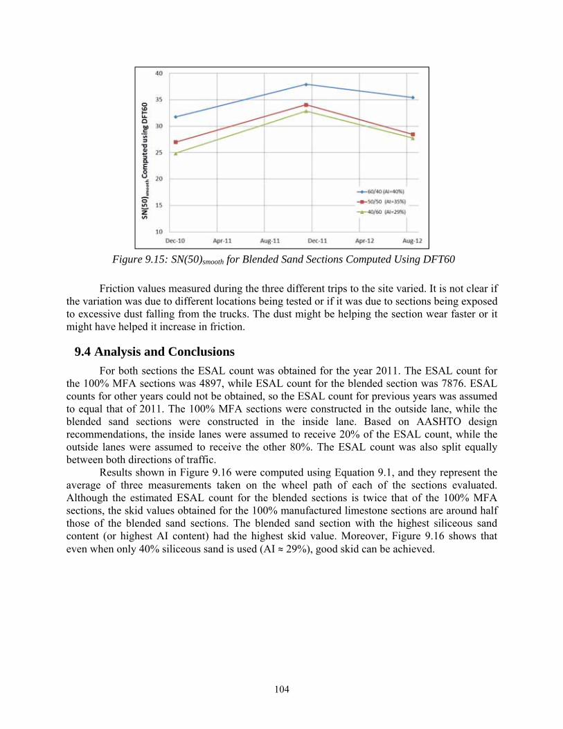
104

Figure 9.15: SN(50)smooth for Blended Sand Sections Computed Using DFT60

Friction values measured during the three different trips to the site varied. It is not clear if the variation was due to different locations being tested or if it was due to sections being exposed to excessive dust falling from the trucks. The dust might be helping the section wear faster or it might have helped it increase in friction.

Analysis and Conclusions 9.4

For both sections the ESAL count was obtained for the year 2011. The ESAL count for the 100% MFA sections was 4897, while ESAL count for the blended section was 7876. ESAL counts for other years could not be obtained, so the ESAL count for previous years was assumed to equal that of 2011. The 100% MFA sections were constructed in the outside lane, while the blended sand sections were constructed in the inside lane. Based on AASHTO design recommendations, the inside lanes were assumed to receive 20% of the ESAL count, while the outside lanes were assumed to receive the other 80%. The ESAL count was also split equally between both directions of traffic.

Results shown in Figure 9.16 were computed using Equation 9.1, and they represent the average of three measurements taken on the wheel path of each of the sections evaluated. Although the estimated ESAL count for the blended sections is twice that of the 100% MFA sections, the skid values obtained for the 100% manufactured limestone sections are around half those of the blended sand sections. The blended sand section with the highest siliceous sand content (or highest AI content) had the highest skid value. Moreover, Figure 9.16 shows that even when only 40% siliceous sand is used (AI ≈ 29%), good skid can be achieved.

105

Figure 9.16: MPD vs. Measured SN(50)smooth

Using a 100% manufactured limestone fine aggregate likely resulted in greater loss of skid resistance than when some siliceous sand was present. Blending a limestone aggregate with a small percentage of siliceous fine aggregate can have a high impact on skid performance. Skid performance seems to increase due to using blends of aggregates with higher siliceous content. Pavements made with lower siliceous content will not necessarily polish and fail, but will have lower skid values when compared to sections with higher siliceous content. The rate of wear of a pavement is also related to the amount of traffic it experiences. The blended sand sections have been in service for more than 16 years. However, because they are located in an inside lane, they have experienced fewer ESALs than they would have if they were located on the outside lane.

106

107

Evaluation of Hardened Concrete Properties Chapter 10.

The effects of aggregates on the hardened properties of concrete were evaluated using standard mixture proportions. In this chapter, the effect of changing fine aggregates on compressive strength, modulus of elasticity, drying shrinkage, and skid resistance were tested for concrete made with different fine aggregates. Thirty-three different fine aggregates as well as six blends were tested for friction. Fifteen out of the thirty-three fine aggregates as well as the six blended mixtures were tested for strength, modulus of elasticity, and drying shrinkage. The reason the other eighteen were not tested for modulus of elasticity and drying shrinkage was that those properties did not correlate with friction results obtained for the original fifteen aggregates tested. Note that all the mixtures evaluated in this chapter had the same mixture proportions, and that they were tested for strength and had a compressive strength of more than 4500 psi after 7 days of curing. The data for skid testing in this chapter is limited to what is needed to perform analysis and make conclusions. However, the full results are presented in Appendix A. Appendix A includes CTM and DFT after every testing interval as well as the computed SN(50)smooth and SN(40)ribbed using the IFI formula (Equations 3.1, 3.2, 3.3, and 3.4) and SN(50)smooth using Equation 9.1.

Mixing and Testing Procedures 10.1

The procedures described in ASTM C 192 were used for mixing concrete. However, when MFAs were used, the mixing time sometimes had to be increased to ensure proper mixing. Also, for the mixtures containing blended sands, the two fine aggregates were added to the mixer and mixed prior to the coarse aggregate. This was done to ensure that the fine aggregates were well blended (each of the fine aggregates was batched separately). As discussed in Chapter 4, a mid-range water-reducing admixture was used to facilitate casting the specimen. The admixture content was varied depending on the fine aggregate and proportions used. The admixture dosage was not recorded since this type of admixture is not usually used in paving concrete; data obtained on admixture content or workability was considered to not be useful.

The compressive strength of concrete was tested at 7 and 28 days following ASTM C 39 procedures using 4-in. x 8-in. cylinders. The modulus of elasticity at 28 days was measured using the procedures described in ASTM C 469 (two cylinders were tested). The method described in ASTM C 157 was used to measure drying shrinkage for 112 days after curing. The concrete tested for shrinkage was not cured for 28 days as specified by ASTM C 157; it was cured for only 7 days. This approach was taken because 7 days of curing better represents curing done in the field (three samples were tested).

Skid resistance was evaluated using the CTM, DFT, and TWPD. Two slabs measuring 20 in. wide and 3 ½ in. deep were tested for each mixture. The change in texture and friction was monitored over 160,000 polishing cycles (3 days of testing per slab). Measurements were taken initially and after 5,000, 40,000, 100,000, and 160,000 polishing cycles. To evaluate the same polished area, each slab was marked so that readings could be taken at the same location (Figure 10.1). All slabs were finished using a broom finish and the surface was cured for at least 28 days before the slabs were tested. Two texture readings were measured using the CTM for each slab at each polishing interval. When measuring friction using the DFT, ASTM E 1911 reports that standard deviation on the same test surface for DFT60 is 0.038. Thus, friction measurements

108

using the DFT at 40,000, 100,000, and 160,000 cycles, were repeated several times on the same slab at the same location until the difference between the last two readings was less than or equal to 0.01. The last measurement obtained (usually the lowest) was reported. Note that after comparing laboratory and field results, it was found that 160,000 TWPD cycles were equivalent to 700,000 ESALs; the derivation of this number is shown in Chapter 12.

Figure 10.1: Typical Markings on a Slab

The black polyurethane wheels described in Chapter 8 were used to polish all slabs tested. Each set of polyurethane wheels lasted about 500,000 cycles (1 wheel per slab). Because those wheels were used, another modification to the TWPD was needed. A vibration dampener was added to TWPD after the TWPD failed several times (Figure 10.2). The failure happened because the wheels used were much stiffer than the original pneumatic wheels that the TWPD was designed for. The stress caused by the wheels on the concrete surface was estimated to be around 50psi (based on the total load and the contact area).

Figure 10.2: Modified Three-Wheel Polishing Device

109

Evaluating the Effect of Fine Aggregates on Hardened Concrete 10.2Properties

Mixture Proportions 10.2.1

One standard concrete mixture was used to evaluate all fine aggregates tested (Table 10.1). The reason this was done was because the effect of changing mixture proportions on skid resistance was not well understood at that time. In Chapter 11, the effect of changing mixture proportions on friction is discussed. The mixture used for all the tests discussed in this chapter was a six-sack mixture with a water-to-cementitious ratio of 0.42 and a sand-to-aggregate ratio of 0.37.

Mixture Proportions used for Evaluating Fine Aggregates Table 10.1:

Materials (Volume %) Cementitious Water Fine Aggregate Coarse Aggregate

10.73 14.20 27.06 46.01

Siliceous Sands vs. Manufactured Sands 10.2.2

The hardened concrete properties of sands obtained from different sources are compared in this section. The results for the compressive strength at 7 and 28 days are shown in Figures 10.3 and 10.4. The average standard deviation between three compressive strength tests performed was 110 psi. All mixtures reached a compressive strength higher than 6000psi after 7 days of curing. Except for the mixture made with Texas Crushed Stone MFA, the compressive strength of concrete made with the different sands was more or less equal at 7 days. The mixture containing Texas Crushed Stone MFA reached a compressive strength of about 8000psi in 7 days. This might have occurred because Texas Crushed Stone has high microfine content. Research done by Fowler et al, (2008) has shown that higher microfine content could lead to higher compressive strengths. Also, compressive strength is mainly controlled by water-to-cement ratio, and although all mixtures were designed to have the same water-to-cement ratio, the moisture corrections done were influenced by the values of absorption obtained. Rogers and Dziedziejko (2007) found that when using ASTM C 128 for measuring absorption, the presence of microfines results in greater multi-laboratory variation than obtained with the same group of laboratories when the fines are removed. The absorption value obtained for Texas Crushed Stone might not be representative of the real absorption capacity of that aggregate. After 28 days of curing, all concrete mixtures reached a compressive strength higher than 7500psi. The mixture made with Texas Crushed Stone reached a compressive strength of around 9000psi.

110

Figure 10.3: Compressive Strength of Concrete Made with Different Sands after 7 Days of

Curing

Figure 10.4: Compressive Strength of Concrete Made with Different Sands after 28 Days of

Curing

Results for the modulus of elasticity tested at 28 days are shown in Figure 10.5. The two aggregates that resulted in a significantly higher modulus of elasticity were Capital Marble Falls and Trinity Kopperl. The modulus of elasticity of concrete made with MFA did not otherwise differ from concrete made with siliceous sand.

111

Drying shrinkage was monitored for all specimens for 112 days. The 112-day shrinkage results are shown in Figure 10.6. Using Lattimore Stringtown in concrete resulted in the highest shrinkage. Lattimore Stringtown had a mineralogy and shape that differed from all other aggregates tested, and that might explain why the shrinkage values obtained using Lattimore Stringtown were different. All other aggregates resulted in shrinkage values that ranged between 300 to 460 µstrain. The use of manufactured carbonate fine aggregates did not have a negative effect on the shrinkage of concrete.

Figure 10.5: Modulus of Elasticity of Concrete Made with Different Sands after 28 Days of

Curing

112

Figure 10.6: Drying Shrinkage of Concrete Made with Different Sands

Texture and friction was measured on concrete slabs made with different fine aggregates using the procedures described in 10.1. The average results for the coefficient of friction at 37 mph (60 km/hr) (DFT60) for the first fifteen aggregates tested are shown in Figure 10.7, while the average results for texture are shown in Figure 10.8. The average difference in MPD between two slabs made from the same material was 0.155 while the difference in DFT60 values was 0.0212. Except for the slabs made with Lattimore Cleburne, the initial coefficient of friction value at 37 mph (60 km/hr) obtained on each of the surfaces made with siliceous sands ranged from around 0.72 to 0.82. The DFT60 value after 160,000 polishing cycles for all the siliceous sands was higher than a coefficient of friction µ of 0.45. After 160,000 cycles, all siliceous sands had DFT60 values that ranged from 0.47 to 0.52.

The MPD values obtained from finishing the surfaces (initial MPD) ranged from 1.3 to 2.05 for all finished surfaces. After only 5,000 polishing cycles, the MPD was reduced to a range of about 0.7 to 1.2. The only slabs that maintained significantly higher MPD values were the slabs made with the Colorado River Sand. Those slabs had higher MPD values because their initial texture was higher; this texture, however, did not seem to contribute to an increase in friction after 160,000 polishing cycles. The reduction in texture between 40,000 cycles and 160,000 cycles was not significant compared to the reduction in texture that occurred after the initial 5,000 cycles.

There were no trends between texture and friction results; while the friction values at 160,000 cycles for all siliceous sands converged to a range of 0.47 to 0.52, the range of texture values was wider (0.55 to 1). Also, between 40,000 and 160,000 cycles, the drop in friction was more significant than the drop in texture.

Note that the reason many siliceous sands were tested was to test how sands having different acid insoluble residue (AI) values above 60% differed. The values obtained in this chapter will be compared to AI in Chapter 11.

113

Figure 10.7: DFT60 Results for Siliceous Sands

Figure 10.8: Texture Results for Siliceous Sands

The results of the friction measurements for the manufactured sands are shown in Figure 10.9. The average difference in DFT60 values between two slabs made from the same material was 0.0262. The initial finished slabs had DFT60 values ranging from 0.52 to 0.85. Compared to the siliceous sands, the values at 160,000 cycles for the manufactured sands were significantly different; they ranged from 0.37 to 0.5 (the siliceous sands ranged from 0.47 to 0.52). Moreover, the slabs that had the highest initial friction did not necessarily maintain it after 160,000 cycles. Lattimore Stringtown started with a DFT60 value of 0.52 and reached a value of 0.48 after 160,000 cycles. Texas Crushed Stone started with an average DFT60 value of around 0.74; this value dropped to 0.37 after 160,000 cycles. The starting friction value for the manufactured sands did seem to affect the final value at 160,000 cycles. The only three MFAs that had a DFT60 value higher than 0.45 were Lattimore Stringtown, Capital Marble Falls, and Hanson Servtex. The values obtained for Hanson Servtex were not expected; Hanson Servtex is a limestone that has shown poor performance in asphalt concrete and was therefore expected to perform as the other three limestone fine aggregates did.

114

After the preliminary testing for skid was performed (discussed in Chapter 8), testing the slabs for 160,000 cycles was considered to be adequate to differentiate between different fine aggregates. After the results for the slabs made with Servtex were obtained, it was decided to test three slabs made with carbonate manufactured sands for an additional 340,000 cycles (a total of 500,000 cycles). The DFT60 results are shown in Figure 10.10. The DFT60 values for the slab made with Capital Marble Falls (dolomite) did not change between 160,000 cycles and 500,000 cycles, while the DFT60 values for the slabs made with the Hanson Servtex (limestone) and Texas Crushed Stone (limestone) slightly dropped. Testing carbonate aggregates beyond 160,000 cycles and not obtaining a significant drop in friction signifies that the polishing capacity of the TWPD using the black polyurethane wheels was reached close to 160,000 cycles.

Figure 10.9: DFT60 Results for Manufactured Sands

Figure 10.10: DFT60 Results for Manufactured Sands Tested for 500,000 Cycles

The texture results for the concrete slabs made with manufactured sands are presented in Figure 10.11. All manufactured sands had an initial texture ranging from an MPD of 1.7 to 1.9. The average difference in MPD between two slabs made from the same material was 0.148. In general, the initial MPD values obtained with the siliceous sands were lower than the initial MPD values obtained using manufactured sands. This might have occurred because using MFA resulted in having more poorly shaped aggregates at the surface and harsher mixtures. The

115

highest MPD value obtained after 160,000 cycles was for the slabs made with TXI Bridgeport. The lowest MPD value obtained was for Hanson Perch Hill.

The texture values after 500,000 cycles for the three slabs made with carbonate aggregates were also evaluated. The results are shown in Figure 10.12. Although Capital Marble Falls maintained the same DFT60 value at 160,000 cycles, the MPD value at 160,000 cycles was not maintained after 340,000 cycles. Both Texas Crushed Stone and Hanson Servtex also did not maintain their texture values after the additional 340,000 cycles.

Note that only three slabs for each mixture were tested for 500,000 cycles. The reason that more slabs were not tested for 500,000 cycles was because 160,000 cycles was sufficient to differentiate between slabs made with different sands and because no significant changes in friction were observed between 500,000 and 160,000 cycles. Moreover, testing for 500,000 cycles takes 7 days for each slab tested, so testing more slabs for that many cycles is unfeasible if such testing is not necessary.

Figure 10.11: Texture Results for Manufactured Sands

Figure 10.12: Texture Results for Manufactured Sands Tested for 500,000 Cycles

116

The DFT60 and the MPD results at 160,000 cycles for all thirty-three tested sands are presented in Figures 10.13 and 10.14. Except for three limestone aggregates, all limestone sands (green bars) had DFT60 values lower than any of the siliceous sands (blue bars). Because the DFT evaluates micro-texture, those values were expected (field performance test have shown that siliceous sands have better skid performance compared to limestone sands). Some of the dolomite aggregates (red bars) had values as high as those of siliceous sands, while others had values comparable to limestones. Unlike the limestones that tested high, the dolomites were expected have good performance. Laboratory results obtained by Balmer and Colley (1966) also showed that dolomitic sands had higher wear indices compared to limestone sands (section 3.2.3.2). However, it is not clear whether such performance could be obtained in the field. TxDOT could not identify any field sections made with 100% dolomite sand because dolomite sands do not meet the AI limit of 60% and for this reason dolomite sands have not been used at 100% replacement for PCC pavements in Texas.

Lattimore Stringtown (slate—black bar) and MM Sawyer (sandstone—brown bar) both meet AI requirements but are not used for pavement concrete. One of the reasons Lattimore Stringtown is not used in PCC pavement is related to its shape. As discussed in Chapter 6, Lattimore Stringtown has a very poor shape which results in poorly workable and finishable concrete.

The expected performance of fine aggregates did not relate well with the texture results obtained in Figure 10.14. The average difference in MPD between two slabs made from the same material at 160,000 cycles was 0.111. The MPD values for all siliceous sands except for the Colorado River Sand at 160,000 cycles were equal or lower than the MPD values obtained for the concrete slabs made with manufactured sands. Poor correlation between macro-texture values obtained using the CTM and micro-texture values obtained using the DFT was expected after the preliminary work on CTM and DFT was done (discussed in Chapter 8). The equivalent skid number using the IFI was computed and can be found in Appendix A. The computed equivalent skid number using the IFI is a factor of the CTM value; for this reason no correlation can be established between that number and the expected performance.

117

Figure 10.13: DFT60 Results at 160,000 Cycles for the Different Sands Tested

118

Figure 10.14: Texture Results at 160,000 Cycles for the Different Sands Tested

Blended Sands 10.3

Fine aggregate that do not meet the AI requirements are blended with sands that have higher AI values to meet the specifications. The current TxDOT specifications require sands to meet an AI value of 60%. Therefore, it was important to evaluate blends of sands that had AI values lower than 60%. For this purpose two different sand combinations with AI values of 20%, 40%, and 60% were tested. One contained TXI Paradise (siliceous) and TXI Bridgeport (limestone), and the other contained Trinity Kopperl (siliceous) and Hanson perch Hill (limestone). The mixture proportions used for making the concrete slabs were the same proportions presented in Table 10.1, but for those mixtures a 30% fly ash replacement was used. There were no indications from the literature reviewed that using fly ash might influence skid

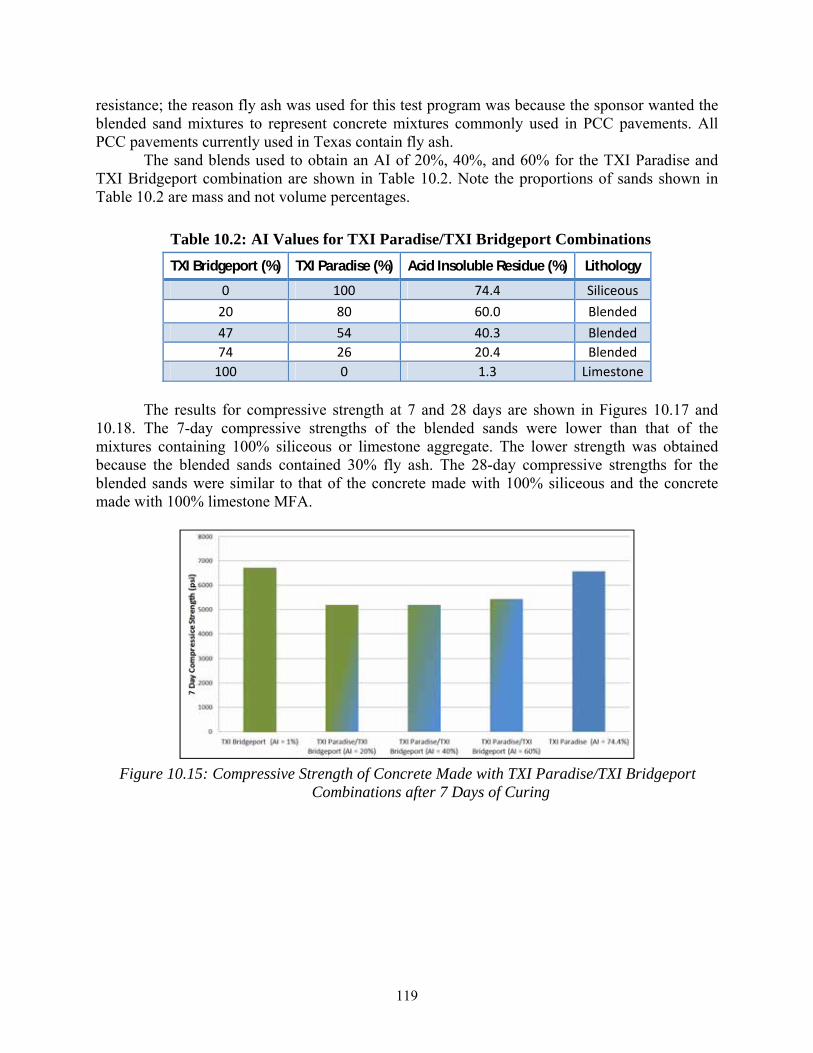
119

resistance; the reason fly ash was used for this test program was because the sponsor wanted the blended sand mixtures to represent concrete mixtures commonly used in PCC pavements. All PCC pavements currently used in Texas contain fly ash.

The sand blends used to obtain an AI of 20%, 40%, and 60% for the TXI Paradise and TXI Bridgeport combination are shown in Table 10.2. Note the proportions of sands shown in Table 10.2 are mass and not volume percentages.

AI Values for TXI Paradise/TXI Bridgeport Combinations Table 10.2:

TXI Bridgeport (%) TXI Paradise (%) Acid Insoluble Residue (%) Lithology 0 100 74.4 Siliceous

20 80 60.0 Blended 47 54 40.3 Blended 74 26 20.4 Blended

100 0 1.3 Limestone The results for compressive strength at 7 and 28 days are shown in Figures 10.17 and

10.18. The 7-day compressive strengths of the blended sands were lower than that of the mixtures containing 100% siliceous or limestone aggregate. The lower strength was obtained because the blended sands contained 30% fly ash. The 28-day compressive strengths for the blended sands were similar to that of the concrete made with 100% siliceous and the concrete made with 100% limestone MFA.

Figure 10.15: Compressive Strength of Concrete Made with TXI Paradise/TXI Bridgeport

Combinations after 7 Days of Curing

120

Figure 10.16: Compressive Strength of Concrete Made with TXI Paradise/TXI Bridgeport

Combinations after 28 Days of Curing

The modulus of elasticity values at 28 days (Figure 10.19) for the blended sands was similar to that of the mixture containing 100% siliceous sand (TXI Paradise). The shrinkage values for the blended sand mixtures were not different from what was obtained when 100% siliceous or limestone aggregate was used (Figure 10.20). Blending sands does not have a large impact on modulus of elasticity or shrinkage.

Figure 10.17: Modulus of Elasticity of Concrete Made with TXI Paradise/TXI Bridgeport

Combinations after 28 Days of Curing

121

Figure 10.18: Drying Shrinkage of Concrete Made with TXI Paradise/TXI Bridgeport

Combinations

The DFT60 and texture results for the TXI Paradise and TXI Bridgeport blends are shown in Figures 10.21 and 10.22. The average difference in MPD between two slabs made from the same material was 0.141 while the difference in DFT60 values was 0.0191. The DFT60 values for the mixtures containing higher siliceous sand content (or higher AI) were higher. The texture values were higher for the mixture containing no siliceous sand. The decrease in friction and texture followed trends similar to what was discussed in 10.2.2.

Figure 10.19: DFT60 Results for TXI Paradise/TXI Bridgeport Combinations

122

Figure 10.20: Texture Results for TXI Paradise/TXI Bridgeport Combinations

The DFT60 values at 160,000 cycles (Figure 10.23) increased as the siliceous content increased. The mixture with an AI of 20% only had 26% siliceous sand but performed almost as well as the mixture with an AI value of 40% which had a siliceous content of 54%. No significant difference was found between the mixture containing 100% siliceous sand and the mixture that had an AI of 60%. All in all, adding a small quantity of siliceous sand had a large effect on skid performance. Note that the average difference in MPD between two slabs made from the same material was at 160,000 cycles was 0.111 while the difference in DFT60 values was 0.0057.

Figure 10.21: DFT60 Results at 160,000 Cycles for TXI Paradise/TXI Bridgeport Combinations

After 160,000 cycles, the texture value of the mixture containing 100% siliceous sand was lower than the texture obtained from all the other mixtures shown in Figure 10.24. The mixture containing 100% TXI Bridgeport had the highest texture after 160,000 polishing cycles.

123

Figure 10.22: Texture Results at 160,000 Cycles for TXI Paradise/TXI Bridgeport Combinations

The sand blends used to obtain an AI of 20%, 40%, and 60% for the Trinity Kopperl and Hanson Perch Hill combination is shown in Table 10.3.

AI Values for Trinity Kopperl/Hanson Perch Hill Combinations Table 10.3:

Hanson Perch Hill (%) Trinity Kopperl (%) Acid Insoluble Residue (%) Lithology

0 100 76.8 Siliceous 24 76 60.0 Blended53 47 39.7 Blended 81 19 20.1 Blended

100 0 6.7 Limestone The results for compressive strength at 7 and 28 days are shown in Figures 10.25 and

10.26. The 7-day compressive strength of the blended sands was lower than that of the mixtures containing 100% siliceous or limestone aggregate. The lower strength was obtained because the blended sands contained 30% fly ash. The 28-day compressive strength for the blended sands was similar to that of the concrete made with 100% siliceous and 100% limestone MFA.

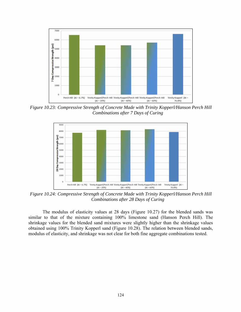
124

Figure 10.23: Compressive Strength of Concrete Made with Trinity Kopperl/Hanson Perch Hill

Combinations after 7 Days of Curing

Figure 10.24: Compressive Strength of Concrete Made with Trinity Kopperl/Hanson Perch Hill

Combinations after 28 Days of Curing

The modulus of elasticity values at 28 days (Figure 10.27) for the blended sands was similar to that of the mixture containing 100% limestone sand (Hanson Perch Hill). The shrinkage values for the blended sand mixtures were slightly higher than the shrinkage values obtained using 100% Trinity Kopperl sand (Figure 10.28). The relation between blended sands, modulus of elasticity, and shrinkage was not clear for both fine aggregate combinations tested.

125

Figure 10.25: Modulus of Elasticity of Concrete Made with Trinity Kopperl/Hanson Perch Hill

Combinations after 28 Days of Curing

Figure 10.26: Drying Shrinkage of Concrete Made with Trinity Kopperl/Hanson Perch Hill

Combinations

The DFT60 and texture results for the Trinity Kopperl and Hanson Perch Hill blends are shown in Figures 10.29 and 10.30. The average difference in MPD between two slabs made from the same material was 0.097 while the difference in DFT60 values was 0.0176. The DFT60 values for the mixtures containing any amount of siliceous sand content were significantly higher than the mixture made with 100% limestone MFA (Hanson Perch Hill). The highest texture values were obtained for the mixture with an AI of 20%.

126

Figure 10.27: DFT60 Results for Trinity Kopperl/Hanson Perch Hill Combinations

Figure 10.28: Texture Results for Trinity Kopperl/Hanson Perch Hill Combinations

The DFT60 values at 160,000 cycles (Figure 10.31) increased for the blended sands as

the siliceous content increased. By only adding 19% Trinity Kopperl (AI of 20%), the DFT60 value was increased from 0.37 to 0.45. This shows that adding a small quantity of siliceous sand to concrete mixtures has a significant effect on friction. Such results are similar to the findings obtained by Balmer and Colley (1966) which indicated that adding 25% siliceous sand would result in satisfactory skid performance. Note that the average difference in MPD between two slabs made from the same material was at 160,000 cycles was 0.066 while the difference in DFT60 value was 0.0056.

127

Figure 10.29: DFT60 Results at 160,000 Cycles for Trinity Kopperl/Hanson Perch Hill

Combinations

There was no trend in the change of texture when different blends of Trinity Kopperl and Hanson Perch Hill were used (Figure 10.32). The highest texture at 160,000 cycles was obtained with a mixture having an AI of 20%; lower texture values were obtained when less or more siliceous sand was used.

Figure 10.30: Texture Results at 160,000 Cycles for Trinity Kopperl/Hanson Perch Hill

Combinations

Conclusions 10.4

The main goal of the concrete testing performed in this research project was to evaluate the skid resistance of concrete made with manufactured sands. While evaluating skid resistance of concrete made with MFA, it was important to ensure that other concrete properties such as compressive strength, shrinkage, and modulus of elasticity were not negatively affected by the use of MFA. Testing yielded the following results:

• The use of manufactured sand in concrete does not lead to a reduction in compressive strength.

128

• Except for the dolomite sand tested, the modulus of elasticity obtained using manufactured sands was higher than that of concrete made with siliceous sand.

• The shrinkage values obtained with all carbonate aggregates was comparable to the shrinkage values obtained using siliceous sands. Concrete made with Lattimore Stringtown had higher shrinkage values than concrete made from all the other sands.

• The texture values (MPD) measured using the CTM did not correlate well with the expected performance of fine aggregates. Concrete made with soft manufactured limestone sands had MPD values that were sometimes higher than the MPD values obtained with concrete made with hard siliceous sands. The MPD value is thus not a good tool for evaluating the polish resistance of fine aggregates.

• The DFT60 values correlated well with the expected skid performance of fine aggregates in concrete. Except for one dolomite, the friction values obtained for the siliceous sands had values higher than all carbonate sands.

• Dolomite sands performed better than the limestone sands.

• Blending a small quantity of siliceous sand with soft limestone manufactured sands considerably increased the DFT60 value after 160,000 polishing cycles.

129

Evaluating the Effect of Mixture Proportions on Texture Chapter 11. and Friction of PCC

The mixtures tested for friction were made with different fine aggregates using the same proportions of materials. Friction testing was performed on mixtures made from the same fine aggregate but having different proportions. The goal of this testing was to investigate whether or not friction performance of carbonate fine aggregates could be improved by modifying mixture proportions. Note that the complete data set for the testing presented in this chapter can be found in Appendix B.

Mixture Proportions 11.1

In Section 10.2, all mixtures were evaluated using the same mixture proportions. This section describes how the effect of changing mixtures proportions was investigated using limestone MFA. The seven different mixture proportions used are shown in Table 11.1.

Mixture Proportions used for Evaluating the Effect of Proportioning on Skid Table 11.1:

Materials (Volume %)

Cement Water Fine Aggregate Coarse Aggregate Baseline Mixture 10.73 14.20 27.06 46.01

W/C = 0.39 11.19 13.74 27.06 46.01 W/C = 0.45 10.31 14.62 27.06 46.01 S/A = 0.3 10.73 14.20 21.92 51.15

S/A = 0.44 10.73 14.20 32.15 40.92 5.25-Sack Mixture 9.30 12.30 28.29 48.11 6.75-Sack Mixture 12.00 15.88 25.97 44.16

Effects of Varying Mixture Proportions on Limestone Sands 11.2

Figures 11.1 and 11.2 show the friction and texture results for the same sand mixed at three different water-to-cement ratios. The initial DFT60 values were not equal. As the numbers of cycles increased, the DFT60 value seemed to converge to the same value for the three different mixtures. Changing the mixture design by varying the water-to-cement ratio between 0.39 and 0.45 does not seem to affect the DFT60 values after 160,000 polishing cycles. The texture values were different for two out of the three mixtures. The highest texture was obtained with the mixture that had the highest water-to-cement ratio.

130

Figure 11.1: DFT60 Results for Mixtures Containing Hanson Perch Hill at Three Different W/C

Ratios

Figure 11.2: Texture Results for Mixtures Containing Hanson Perch Hill at Three Different

W/C Ratios

Figures 11.3 and 11.4 show the friction and texture results for the same sand mixed at three different sand-to-aggregate ratios. Changing the sand-to-aggregate ratio from 0.30 to 0.44 had no effect on the DFT60 value at 160,000 cycles. The DFT60 value seemed to have converged at 100,000 cycles, even though the starting values were not equal. As for texture, the mixture that had the lowest sand-to-aggregate ratio had the lowest texture; this might be due to the fact that that mixture had less sand which resulted in a concrete texture containing less poorly shaped particles.

131

Figure 11.3: DFT60 Results for Mixtures Containing TXI Bridgeport at Three Different S/A

Ratios

Figure 11.4: Texture Results for Mixtures Containing TXI Bridgeport at Three Different S/A

Ratios

Figures 11.5 and 11.6 show the friction and texture results for the same sand mixed at with different cement content. Increasing or decreasing cement content did not improve the DFT60 value of mixtures made with TXI Bridgeport. The DFT60 values measured converged after 160,000 polishing cycles. Results obtained in Figure 11.6 show that the mixtures with the highest cement content had the lowest initial texture and the lowest texture at 160,000 cycles. This might have occurred due to a change in fine aggregate content; as the cement content changed the paste content had to also be changed to maintain a constant water-to-cement ratio. This caused the total aggregate ratio to either decrease or increase when the cement content was changed (Table 11.1). As the fine aggregate content decreased, less texture was created because the mixtures had less poorly shaped fine aggregate and were not as harsh (had higher paste content).

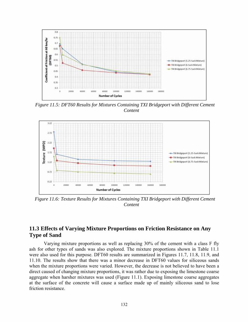
132

Figure 11.5: DFT60 Results for Mixtures Containing TXI Bridgeport with Different Cement

Content

Figure 11.6: Texture Results for Mixtures Containing TXI Bridgeport with Different Cement

Content

Effects of Varying Mixture Proportions on Friction Resistance on Any 11.3Type of Sand

Varying mixture proportions as well as replacing 30% of the cement with a class F fly ash for other types of sands was also explored. The mixture proportions shown in Table 11.1 were also used for this purpose. DFT60 results are summarized in Figures 11.7, 11.8, 11.9, and 11.10. The results show that there was a minor decrease in DFT60 values for siliceous sands when the mixture proportions were varied. However, the decrease is not believed to have been a direct caused of changing mixture proportions, it was rather due to exposing the limestone coarse aggregate when harsher mixtures was used (Figure 11.1). Exposing limestone coarse aggregates at the surface of the concrete will cause a surface made up of mainly siliceous sand to lose friction resistance.

133

Figure 11.7: Effects of Varying W/C Ratio on DFT60 Values after 160,000 TWPD Cycles

Figure 11.8: Effects of Varying Sand/Aggregate Ratio on DFT60 Values after 160,000 TWPD

Cycles

134

Figure 11.9: Effects of Varying Paste Content on DFT60 Values after 160,000 TWPD Cycles

Figure 11.10: Effects of Using Fly Ash on DFT60 Values after 160,000 TWPD Cycles

135

Figure 11.11: Concrete Slab with Exposed Limestone Coarse Aggregate

Effects of Adding Water onto the Concrete Surface 11.4

The 100% MFA sections discussed in Chapter 9 had lower skid numbers than the sections made with blended sands mainly because they only contained a source of limestone sand that is prone to polishing. However, the wear on the wheel path that was observed was not due to presence of limestone sand, but due to the poor finishing of the surface. To be able to finish the concrete surface the finishers had to spray the surface with water. This probably diluted the cement paste at the surface, thus causing it to polish in less than a year. Several test slabs were made with TXI Bridgeport fine aggregate; In addition to the baseline (control) mixture, several variables were used:

• Use of fly ash;

• Low and high sand content;

• Low and high paste content; and

• Two amounts of water added to the surface. Table 11.2 shows the results obtained. Slabs that started with a higher DFT60 value did

not necessarily end up with a higher DFT60 value after 160,000 TWPD cycles. Moreover, it has been found earlier in this research that the type of finishing applied on the mortar, whether it is a carpet, turf, or broom finish does not have a significant effect on the DFT60 value after 160,000 polishing cycle. These results proved that changing mixture proportions had only a minor effect on the DFT60 value after 160,000 polishing cycles, but adding water to surface and working it into the paste during finishing caused the DFT60 value to drop by around 10%. Although it is unknown how much water was added to the surface of the field sections, the samples made at the laboratory with the addition of water on the surface better represent the field test sections.

136

DFT60 Results for Concrete Slabs made with TXI Bridgeport Sand Table 11.2:

TXI Bridgeport Mixtures DFT60 initial values (0 cycles) DFT60 after 160,000 Cycles

Baseline 0.676 0.422

Baseline (30% fly ash) 0.753 0.409

Low sand content 0.629 0.414

High sand content 0.718 0.421

Low paste content 0.694 0.433

High paste content 0.750 0.429

Average 0.703 0.421

Baseline + water added to surface (11 oz/yd2)

0.687 0.39

Baseline + water added to surface (22 oz/yd2)

0.836 0.373

Average of Samples with added water to the surface

0.761 0.3815

Conclusions 11.5

Based on the results presented in this chapter, several conclusions can be made concerning the effect of mixture proportioning on friction resistance, these can be summarized as follows:

• Changing mixture proportions might have an effect on macro-texture (MPD values) but it did not have any effect on the DFT60 values after 160,000 TWPD cycles when limestone MFAs were used. Thus, the performance of limestone MFAs cannot be improved by changing mixture proportions. As much as the macro-texture could potentially be improved, the micro-texture is controlled by the type of fine aggregate used.

• Changing concrete proportions does not have a direct effect on friction, but it might have an indirect negative effect. If a mixture is too rocky or too harsh, coarse aggregate might be exposed at the surface. If the exposed coarse aggregate is soft, it will polish and cause a drop in friction even if 100% siliceous sand was used in the mixture.

• Adding water onto the surface of the concrete will raise the water-to-cement ratio at the surface of the concrete. Mortar paste with higher water-to-cement ratios polish faster; thus, the macro-texture will be lost much quicker than intended.

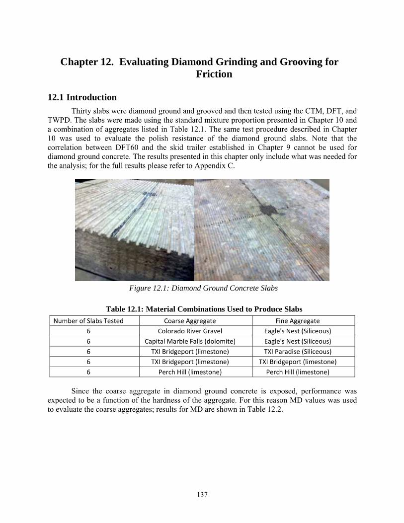
137

Evaluating Diamond Grinding and Grooving for Chapter 12. Friction

Introduction 12.1

Thirty slabs were diamond ground and grooved and then tested using the CTM, DFT, and TWPD. The slabs were made using the standard mixture proportion presented in Chapter 10 and a combination of aggregates listed in Table 12.1. The same test procedure described in Chapter 10 was used to evaluate the polish resistance of the diamond ground slabs. Note that the correlation between DFT60 and the skid trailer established in Chapter 9 cannot be used for diamond ground concrete. The results presented in this chapter only include what was needed for the analysis; for the full results please refer to Appendix C.

Figure 12.1: Diamond Ground Concrete Slabs

Material Combinations Used to Produce Slabs Table 12.1:

Number of Slabs Tested Coarse Aggregate Fine Aggregate 6 Colorado River Gravel Eagle's Nest (Siliceous) 6 Capital Marble Falls (dolomite) Eagle's Nest (Siliceous) 6 TXI Bridgeport (limestone) TXI Paradise (Siliceous) 6 TXI Bridgeport (limestone) TXI Bridgeport (limestone) 6 Perch Hill (limestone) Perch Hill (limestone)

Since the coarse aggregate in diamond ground concrete is exposed, performance was

expected to be a function of the hardness of the aggregate. For this reason MD values was used to evaluate the coarse aggregates; results for MD are shown in Table 12.2.

138

Micro-Deval Values for Coarse Aggregates used in Slabs Table 12.2:

Colorado

River Gravel Capital Aggregate Marble Falls (Coarse Aggregate)

Hanson Perch Hill (Coarse Aggregate)

TXI Bridgeport (Coarse Aggregate)

Lithology Siliceous Dolomite Limestone Limestone

Micro-Deval (% loss)

9.6 12.5 13.8 15

The slabs evaluated at the laboratory were diamond ground using four different

configurations. The blade configurations used are presented in Table 12.3, and the resulting concrete surfaces produced are illustrated in Figure 12.1.

Blade Configuration Used to Produce slabs Table 12.3:Number of

Slabs Blade

Configuration # Type of Diamond-grinding

10 1 .125 blades with .130 spacers 10 2 .125 blades with .110 spacers

5 3 Specialized segments that create a surface texture due to the segment

design. The texture created consists of very close spaced fine land areas.

5 4 Specialized segments that create a surface texture due to the segment

design + grooved on 3/4 inch centers with .125 blades and 1/8 inch depth.

Figure 12.2: Illustrations of Surfaces Produced by Diamond Grinding and Grooving

139

Results 12.2

The initial measurements taken on the diamond ground slabs show that higher friction values were obtained when larger land areas were used to grind (larger spacers produce larger land areas). Texture values for the surface produced only with specialized blades had the lowest texture. There does not seem to be any correlation between MPD and DFT60. The MPD texture value for the grooved slab is high because the grooves are deeper than the ground surfaces. The textures produced using the specialized blades produced the most consistent surfaces (almost the same MPD values)

Figure 12.3: Initial DFT60 Values

Figure 12.4: Initial MPD Values

After 160,000 TWPD cycles, the slabs made with the harder aggregates, i.e., the river gravel and the dolomite produced had the highest friction values regardless of the method of grinding. Overall, the slabs made with Perch hill coarse aggregate had the lowest friction values. Note that based on the MD values (Table 12.2), Perch Hill was expected to perform better than TXI Bridgeport. For any aggregate, the highest DFT60 values were obtained with the slabs that had larger land areas.

140

Figure 12.5: DFT60 Values after 160,000 TWPD Cycles

All Tested slabs had a very similar MPD values after 160,000 cycles except the slabs that were grooved. The goal of grooving is to produce deeper cuts that serve as channels that carry water away from pavements to prevent hydroplaning.

Figure 12.6: CTM Values after 160,000 TWPD Cycles

Conclusions 12.3Following are some of the conclusions reached via the results described in this chapter: • Slabs produced using the larger spacers resulted in larger land areas. • Larger land areas produced better friction values initially and after 160,000 TWPD

cycles. • After 160,000 TWPD cycles, harder aggregates had higher friction values. • The TWPD was not able to reduce the texture produced by grooving, and thus there

was no significant drop in the MPD values of the ground and grooved surfaces. • Except for the limestone coarse aggregates tested, MD was able to predict which of the

aggregates performed better.

141

Analysis of Skid Data, Blending Recommendations, and Chapter 13. Development of a Skid Prediction Model for Concrete

Pavements

The concrete testing discussed in Chapter 10 evaluated the polish resistance of 78 slabs made with 33 different fine aggregate and fine aggregate blends. The results showed that the polish resistance of concrete is mainly influenced by the type or blend of sands used. The results from Chapters 8 and 10 showed that friction values measured using the DFT could be used to better evaluate the polish resistance of fine aggregates. In this chapter, the results obtained from the concrete skid tests in Chapter 10 are compared to the aggregate test results presented in Chapter 4. This chapter addresses the goal of finding an aggregate test that can predict skid performance. A formula that relates DFT60 to AI and the MD percent loss was computed. Recommendations for an alternative method of evaluating and blending fine aggregates for pavement concrete is also presented in this chapter. This method aims at better quantifying the hardness of aggregates using MD by evaluating the resistance of fine aggregates to abrasion and crushing rather than their resistance to acid.

Alternative Method for Identifying Polish Resistant Sands 13.1

Analysis of Data 13.1.1

The goal of the laboratory testing was to evaluate the polish resistance of concrete slabs made with different fine aggregates and to relate those results to aggregate tests. The CTM and DFT were used along with a three-wheel polishing device (TWPD) to evaluate the polish resistance of a laboratory concrete specimen.

In Figure 13.1, results of DFT60 after 160,000 polishing cycles on concrete specimens are compared to the AI values of aggregate used. Figure 13.1 shows that some of the carbonate aggregates that had low AI performed as well as the aggregates that had a high AI. There does seem to be a relation between AI and the performance of siliceous and blended aggregates; as the AI decreases, DFT60 values after 160,000 cycles decrease for siliceous and blended aggregates. The relation between AI and DFT60 values for carbonate aggregates (limestone or dolomite) is not clear. A few of the aggregates with AI < 60 % maintained a relatively high DFT60 value after 160,000 polishing cycles.

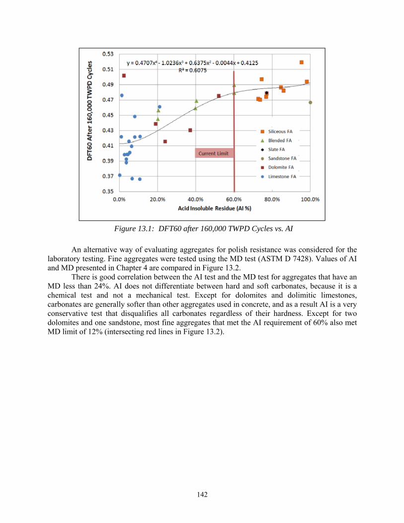
142

Figure 13.1: DFT60 after 160,000 TWPD Cycles vs. AI

An alternative way of evaluating aggregates for polish resistance was considered for the laboratory testing. Fine aggregates were tested using the MD test (ASTM D 7428). Values of AI and MD presented in Chapter 4 are compared in Figure 13.2.

There is good correlation between the AI test and the MD test for aggregates that have an MD less than 24%. AI does not differentiate between hard and soft carbonates, because it is a chemical test and not a mechanical test. Except for dolomites and dolimitic limestones, carbonates are generally softer than other aggregates used in concrete, and as a result AI is a very conservative test that disqualifies all carbonates regardless of their hardness. Except for two dolomites and one sandstone, most fine aggregates that met the AI requirement of 60% also met MD limit of 12% (intersecting red lines in Figure 13.2).

143

Figure 13.2: AI vs. MD

It should be noted that the AI test is only a surrogate test for evaluating the polish resistance of fine aggregates in PCCP, and the test was originally developed based on an observation that an increase in non-carbonate content improves skid resistance (Balmer and Colley). The concrete test results obtained by Balmer and Colley in 1966 also seem to indicate that dolomites perform better than limestone fine aggregates (note that limestones are referred to as calcites in this paper; see Figure 13.3).

144

Figure 13.3: Wear Index Obtained for Different Mineralogies (Balmer and Colley, 1966)

Figure 13.4 shows the relationship between DFT60 after 160,000 TWPD cycles and MD. Regardless of the type of aggregate, the MD test seems to have better correlation with DFT60 than AI. Note that some research has indicated that higher content of shale or chert in an aggregate sample could lead to higher MD percent loss [Hudec and Boateng 1995]. That might explain why some aggregates had a high MD loss but still performed well. Moreover, DFT60 values seem increase as the MD percent loss decreases for aggregates that have an MD loss lower than 24%; aggregates with an MD loss higher than 24% do not seem to follow that trend.

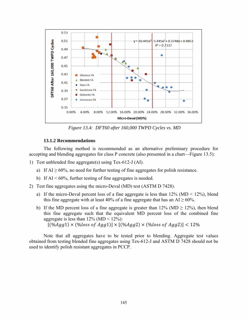
145

Figure 13.4: DFT60 after 160,000 TWPD Cycles vs. MD

Recommendations 13.1.2

The following method is recommended as an alternative preliminary procedure for accepting and blending aggregates for class P concrete (also presented in a chart—Figure 13.5):

1) Test unblended fine aggregate(s) using Tex-612-J (AI).

a) If AI ≥ 60%, no need for further testing of fine aggregates for polish resistance.

b) If AI < 60%, further testing of fine aggregates is needed.

2) Test fine aggregates using the micro-Deval (MD) test (ASTM D 7428).

a) If the micro-Deval percent loss of a fine aggregate is less than 12% (MD < 12%), blend this fine aggregate with at least 40% of a fine aggregate that has an AI ≥ 60%.

b) If the MD percent loss of a fine aggregate is greater than 12% (MD ≥ 12%), then blend this fine aggregate such that the equivalent MD percent loss of the combined fine aggregate is less than 12% (MD < 12%): (% 1) × (% 1) × (% 2) × (% 2) 12% Note that all aggregates have to be tested prior to blending. Aggregate test values

obtained from testing blended fine aggregates using Tex-612-J and ASTM D 7428 should not be used to identify polish resistant aggregates in PCCP.

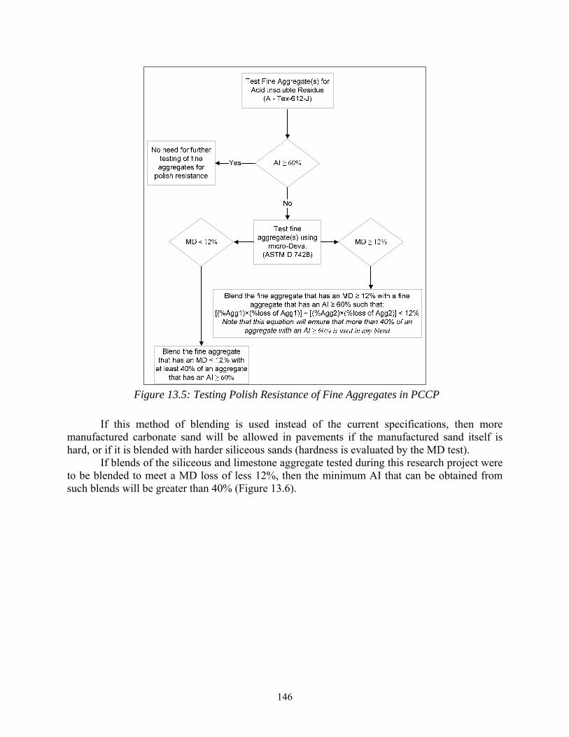
146

Figure 13.5: Testing Polish Resistance of Fine Aggregates in PCCP

If this method of blending is used instead of the current specifications, then more manufactured carbonate sand will be allowed in pavements if the manufactured sand itself is hard, or if it is blended with harder siliceous sands (hardness is evaluated by the MD test).

If blends of the siliceous and limestone aggregate tested during this research project were to be blended to meet a MD loss of less 12%, then the minimum AI that can be obtained from such blends will be greater than 40% (Figure 13.6).

147

Figure 13.6: AI Values for Blends of Aggregates Meeting the 12% MD Limit

Developing a Prediction Model 13.2

Introduction 13.2.1

A model for predicting skid values for concrete pavements is presented in this section. The model was derived using data obtained from the monitored field sections as well as the friction testing conducted at the laboratory. Since all the sections evaluated had a tined and carpet drag finish, the model derived is only suitable for concrete pavements that have a mortar surface exposed to traffic (the effect of exposed coarse aggregate is not accounted for in this model).

Among the twelve sections evaluated, only four sections have been monitored for an extended period. Five of the twelve sections were recently constructed and have not been exposed to a significant amount of traffic; for this reason, data obtained from those sections was not adequate for computing the model. The three sections constructed in 1995 were only used to verify the model; although friction measurements were taken between wheel paths to estimate initial conditions of the sections, it is not clear whether those measurements represent the initial skid resistance of the pavement.

Field Data Analysis 13.2.2

The 100% MFA test sections constructed in 2008 were monitored for three years. CTM and DFT measurements were taken during four visits to the site and the values were converted using Equation 9.1. Measurements taken between the wheel paths are generally not exposed to traffic and were assumed to represent the initial conditions of the pavement. The data obtained are shown in Figure 13.7.

148

Figure 13.7: Computed Skid Numbers for Trial Field Sections as a Function of Time

Sections 1 and 2 were constructed using 100% manufactured limestone aggregate on the outside lane. Section 1 had 5% microfine content while section 2 had 10%. Section 3 was constructed on the inside lane using 100% carbonate aggregate but had 15% microfines (same fine aggregate source as sections 1 and 2). Section 4, the control section on the inside lane, which had a blend of 50/50 is estimated to have an AI of 40%, while the AI of the other three sections can be assumed to be equal to 0%. The manufactured sand used in all the test sections was TXI Bridgeport.

Figure 13.8 shows that a change in microfine content (gradation change) did not have any effect on skid resistance. Even though section 2 had slightly higher initial skid values, sections 1 and 2 had very similar skid values after more than 1 year of traffic. Results obtained from Figure 13.8 also show that trucks have a higher wearing and polishing effect on pavements. The inside lane and the outside lane might have the same average daily traffic (ADT) count but they almost assuredly have different ESAL counts. If the ESAL count is assumed to be the controlling factor in wear and if it is assumed that section 3 had a wear factor similar to sections 1 and 2, then the ESAL distribution between the two lanes can be estimated by matching the wear rate of section 3 with sections 1 and 2. Figure 13.9 shows that a good fit can be obtained if a 77.5/22.5 split is assumed between the outside lane and the inside lane.

149

Figure 13.8: Computed Skid Numbers for Trial Field Sections as a Function of ESALs

Effect of Mixture Variables on Surface Friction 13.2.3

The fine aggregate used in the test sections constructed in 2008 was obtained from the TXI Bridgeport quarry. Figure 13.9 shows the results of three MD coarse aggregate tests for TXI Bridgeport coarse aggregate samples obtained at different times in other research studies. The results show that the three samples obtained from the quarry in 2008, 2009, and 2012 did not vary significantly in hardness. In summer 2010, a sample of fine aggregate from TXI Bridgeport was obtained and tested using the TWPD, CTM, and DFT. The sample tested at the laboratory was obtained from the quarry on a different date than the date the test sections were constructed, but because the hardness of the aggregate has not significantly changed, the fine aggregate used in the field sections and the laboratory tests were assumed to be identical.

Figure 13.9: Relationship between DFT60 after 160,000 TWPD Cycles and AI

150

When the test sections containing 100% MFA were constructed, finishing problems were encountered. The concrete received on site did not meet slump requirements and the finishing crew had trouble finishing it. To be able to finish the concrete, the finishing crew sprayed the surface with water and worked the water into the paste to make the surface more finishable. In Chapter 11 something similar to what was done in the field was tested at the laboratory; those results will be assumed to better correlate with the trial sections.

Relationship between DFT and MD 13.2.4

In Figure 13.1, the values of DFT60 after 160,000 polishing cycles were compared to the MD percent loss of the fine aggregates. Fine aggregate with a MD loss higher than 24% did not follow the trend of decrease in performance with an increase in loss; these limestone fine aggregates might have had materials such as chert that caused them to experience higher loss in MD compared to other limestone fine aggregates. For this reason they were not used to obtain the relationship shown in Figure 13.10.

Figure 13.10: Relationship between DFT60 after 160,000 TWPD Cycles and MD

DFT60 at a 160,000 cycles can be estimated from MD using the following equation: 60 = 0.4717 + 0.4943 × − (3.8446 × ) (Eq. 13.1) = % 1 × + % 2 × (Eq. 13.2)

is the equivalent MD percent loss of two or more fine aggregates. , , and are in percent for the equations presented, i.e., if was equal to 12%, use = = 0.12 in Equation 13.1.

151

Relationship between DFT and AI 13.2.5

DFT60 after 160,000 polishing cycles was compared to the fine aggregates AI values in Figure 13.4. AI evaluates the carbonate content of a fine aggregate and this was the reason the AI values obtained for the dolomitic fine aggregates did not correlate with DFT60. To compute a better relationship between AI and DFT60 at 160,000 cycles, all the dolomites, dolomitic limestones, and carbonates that had DFT60 values comparable to siliceous and blended sands were not considered in Figure 13.11.

Figure 13.11: Relationship between DFT60 after 160,000 TWPD Cycles and AI

DFT60 at a 160,000 cycles can be estimated from AI using the following equation: 60 = 0.3799 + (0.3786 × ) − 0.4901 × + (0.2226 × ) (Eq. 13.3) = % 1 × + % 2 × (Eq. 13.4)

is the equivalent AI of two or more fine aggregates. , , and are in percent for the equations presented, i.e., if was equal to 60%, use a value of == 0.6 in Equation 13.3.

Prediction Model for Computing SN(50)smooth 13.2.6

Figures 13.12, 13.13, and 13.14 represent a wear model for the four different sections tested. Sections 1 and 2 have very similar values and can be represented in one equation. Section 3 can be represented in a model very similar to 1 and 2. Comparing the laboratory test for the slabs made with TXI Bridgeport where water was added to surface and the field results in Figures 13.12 and 13.13 show that 160,000 TWPD cycles are equivalent to around 700,000 ESALs.

152

Figure 13.12: Computed Skid Numbers as a Function of ESALs (Sections 1 and 2)

Figure 13.13: Computed Skid Numbers as a Function of ESALs (Section 3)

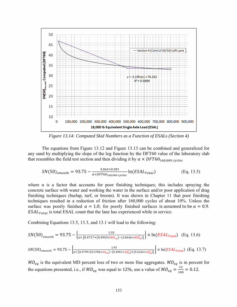
153

Figure 13.14: Computed Skid Numbers as a Function of ESALs (Section 4)

The equations from Figure 13.12 and Figure 13.13 can be combined and generalized for any sand by multiplying the slope of the log function by the DFT60 value of the laboratory slab that resembles the field test section and then dividing it by × 60 ,

(50) = 93.75 − . × .× , ln( ) (Eq. 13.5)

where α is a factor that accounts for poor finishing techniques; this includes spraying the concrete surface with water and working the water in the surface and/or poor application of drag finishing techniques (burlap, turf, or broom). It was shown in Chapter 11 that poor finishing techniques resulted in a reduction of friction after 160,000 cycles of about 10%. Unless the surface was poorly finished = 1.0; for poorly finished surfaces isassumedtobe = 0.9.

is total ESAL count that the lane has experienced while in service. Combining Equations 13.5, 13.3, and 13.1 will lead to the following: (50) ℎ = 93.75 − 1.93× 0.4717+ 0.4943× −(3.8446× 2 ) × ln( ) (Eq. 13.6) (50) = 93.75 − .× . . × . × . × × ln( ) (Eq. 13.7)

is the equivalent MD percent loss of two or more fine aggregates. is in percent for

the equations presented, i.e., if was equal to 12%, use a value of = = 0.12.

154

is the equivalent AI of two or more fine aggregates. is in percent for the equations

presented, i.e., if was equal to 60%, use a value of = = 0.6

Equations 13.6 and 13.7 can be used to predict the skid number of any mortar finished pavement by knowing either the AI or MD and the total ESAL count for the lane. Note that neither equation presented takes into account the presence of exposed coarse aggregates, whether those were intentionally or unintentionally exposed.

Verification of Prediction Model and Development of Design Charts 13.2.7

Equation 13.7 was used to estimate the skid number of four of the sections evaluated. The results are shown in Table 13.1. Note that the exact ESAL count per lane is not known and was assumed to be 20% for sections in location 2. For location 1, 22.5% deduced by matching wear rate between sections 1, 2, and 3. The values predicted in Table 13.1 were not exact for all the sections but were still able to give a conservative estimate of what skid numbers to expect for the different blends.

Verification of the Prediction Model Table 13.1:

Test Section AI (%) Measured SN(50)smooth

Estimated Total ESALs at time of

Skid Test

Estimated Using SN(50)smooth

Model Location 1 - Section 4

(Control 50/50) 40 38.3 670,000 38.3

Location 2 - Blend 60/40 40 37.0 4,600,000 30.4 Location 2 - Blend 50/50 35 29.0 4,600,000 29.6 Location 2 - Blend 40/60 29 33.0 4,600,000 28.5

Equations 13.6 and 13.7 can also be used to calculate the estimated number of years to reach a target skid number as a function of the number of daily lane ESALs and either the MD or AI of the fine aggregate. Tables 13.2, 13.3, 13.4, and 13.5 were developed assuming that the target skid number was (50) = 25. Note that the ESAL values shown in the table are ESALs per lane per day, i.e., the ESAL distribution per lane should be computed before using the tables.

155

Design Chart Assuming ( ) = , Well Finished, and Using AI Table 13.2:

AI (%) Estimated years to reach SN(50)smooth

1% 10% 20% 30% 40% 50% 60% 70% 80% 90% 100%ESALs/lane (per day)

500 5 13 32 61 92 120 139 152 163 180 216 1000 2 7 16 30 46 60 70 76 82 90 108 1500 2 4 11 20 31 40 46 51 54 60 72 2000 1 3 8 15 23 30 35 38 41 45 54 2500 1 3 6 12 18 24 28 30 33 36 43 3000 1 2 5 10 15 20 23 25 27 30 36 3500 1 2 5 9 13 17 20 22 23 26 31 4000 1 2 4 8 12 15 17 19 20 23 27 4500 1 1 4 7 10 13 15 17 18 20 24 5000 0 1 3 6 9 12 14 15 16 18 22 5500 0 1 3 6 8 11 13 14 15 16 20 6000 0 1 3 5 8 10 12 13 14 15 18 6500 0 1 2 5 7 9 11 12 13 14 17

Design Chart Assuming ( ) = , Poorly Finished, and Using AI Table 13.3:

AI (%) Estimated years to reach SN(50)smooth

1% 10% 20% 30% 40% 50% 60% 70% 80% 90% 100%ESALs/lane (per day)

500 1 3 7 12 18 22 25 27 29 32 38 1000 1 2 3 6 9 11 13 14 15 16 19 1500 0 1 2 4 6 7 8 9 10 11 13 2000 0 1 2 3 4 6 6 7 7 8 9 2500 0 1 1 2 4 4 5 5 6 6 8 3000 0 1 1 2 3 4 4 5 5 5 6 3500 0 0 1 2 3 3 4 4 4 5 5 4000 0 0 1 1 2 3 3 3 4 4 5 4500 0 0 1 1 2 2 3 3 3 4 4 5000 0 0 1 1 2 2 3 3 3 3 4 5500 0 0 1 1 2 2 2 2 3 3 3 6000 0 0 1 1 1 2 2 2 2 3 3 6500 0 0 1 1 1 2 2 2 2 2 3

156

Design Chart Assuming ( ) = , Well Finished, and Using MD Table 13.4:

MD (%) Estimated years to reach SN(50)smooth

26% 24% 22% 20% 18% 16% 14% 12% 10% 8% 6% ESALs/lane (per day)

500 1 3 7 15 31 55 87 125 161 185 1911000 1 1 3 8 15 27 44 63 80 93 95 1500 0 1 2 5 10 18 29 42 54 62 64 2000 0 1 2 4 8 14 22 31 40 46 48 2500 0 1 1 3 6 11 17 25 32 37 38 3000 0 0 1 3 5 9 15 21 27 31 32 3500 0 0 1 2 4 8 12 18 23 26 27 4000 0 0 1 2 4 7 11 16 20 23 24 4500 0 0 1 2 3 6 10 14 18 21 21 5000 0 0 1 2 3 5 9 13 16 19 19 5500 0 0 1 1 3 5 8 11 15 17 17 6000 0 0 1 1 3 5 7 10 13 15 16 6500 0 0 1 1 2 4 7 10 12 14 15

Design Chart Assuming ( ) = , Poorly Finished, and Using MD Table 13.5:

MD (%) Estimated years to reach SN(50)smooth

26% 24% 22% 20% 18% 16% 14% 12% 10% 8% 6%ESALs/lane (per day)

500 0 1 2 3 6 11 17 23 29 33 34 1000 0 0 1 2 3 5 8 11 14 16 17 1500 0 0 1 1 2 4 6 8 10 11 11 2000 0 0 0 1 2 3 4 6 7 8 8 2500 0 0 0 1 1 2 3 5 6 7 7 3000 0 0 0 1 1 2 3 4 5 5 6 3500 0 0 0 0 1 2 2 3 4 5 5 4000 0 0 0 0 1 1 2 3 4 4 4 4500 0 0 0 0 1 1 2 3 3 4 4 5000 0 0 0 0 1 1 2 2 3 3 3 5500 0 0 0 0 1 1 2 2 3 3 3 6000 0 0 0 0 1 1 1 2 2 3 3 6500 0 0 0 0 0 1 1 2 2 3 3

157

Conclusions 13.3

The following conclusions and outcomes resulted from the research on achieving adequate surface friction:

• An equation to calculate the skid number based on the skid trailer using a smooth tire at 50 mph (SN (50) smooth) was developed using values obtained by the dynamic friction tester (DFT60) at 60 kmh.

• Based on field test sections using limestone manufactured sands, ranging from 40 to 100% of the total sand, 100% sand gave low skid numbers compared to blended sands.

• There is a reasonable correlation between surface friction based on the DFT and acid insoluble residue values (AI) for all aggregates and blends except dolomites and dolomitic limestones. For AI > 60%, friction values were high, but even for some fine aggregates at AI < 60% relatively high friction values were achieved.

• A good correlation exists between MD loss and AI for aggregates with MD less than 24%. Hard fine aggregates such as some dolomites and dolomitic limestones performed well when tested for friction using the TWPD.

• An alternative method to the current TxDOT acceptance procedure for use of fine aggregates in class P concrete is proposed based on MD. This method allows harder MFA that do not meet AI to be used at a higher replacement rate without causing reductions in skid on pavements. An MD limit of 12% loss was recommended for the new procedures,

• Using field and laboratory data, a model for predicting skid was established. The model allows SN(50)smooth to be estimated by knowing the total ESAL count and the AI or MD value of the pavement.

• The model established for predicting SN(50)smooth was used to develop design tables that can aid designers in choosing what AI or MD limits they need to follow, given the ESAL count and the approximate number of years they need a pavement to maintain a desired value of SN(50)smooth.

158

159

Summary and Conclusions Chapter 14.

Summary 14.1

The goal of this project was to investigate the use of manufactured sands in pavement concrete. This topic was investigated because there is an increasing need to use more local materials such as manufactured fine aggregates (MFAs) that do not meet current specifications. The main concrete properties affected by the usage of MFAs are skid resistance, workability, and finishability. Skid resistance in portland cement concrete (PCC) pavements is mainly a problem associated with the mineralogy of the sand. Many available sources of manufactured sands are soft carbonate aggregates; those aggregates polish when used in PCC pavement. Workability and finishability are problems associated with the shape and grading of the fine aggregates used for making concrete. To obtain more workable and finishable concrete, the shape and grading of the aggregates has to be improved, or an optimized proportioning method that accounts for the poor shape and grading of those aggregates needs to be used. The research performed in this project investigated some of those issues. This section provides a summary of the different topics discussed in this dissertation.

Finding a Fine Aggregate Test that Predicts Skid Performance 14.1.1

The acid insoluble residue (AI) test currently used by TxDOT and other state agencies is a surrogate test that measures the carbonate content of fine aggregates. The AI does not directly measure the hardness of the aggregate. The use of the micro-Deval (MD) abrasion test for fine aggregates was explored. The time of the test was varied to determine whether better results could be obtained. Results showed that the 15-minute run time adopted by ASTM seems to give better results than the longer times attempted—when the MD was run for longer periods, more crushing of fine aggregates occurred.

Testing hardened mortar specimens in the MD might be a better way of evaluating polish resistant aggregates because it better simulates abrasion of fine aggregates in concrete. The problem encountered while testing mortar specimens with the MD was that the abraded specimens had air voids that influenced the texture readings. Attempts to de-air the concrete worked, but fewer aggregates were exposed by the MD, so no consistent texture readings could be made on those specimens. Moreover, AIMS was found to evaluate the color of the exposed aggregate rather than texture; a better tool for evaluating texture was not available. The ASTM MD test was the only MD test that was compared to concrete results.

Evaluating the Shape of MFA Produced Using Different Crushing Operations 14.1.2

To determine whether improvement in shape could be obtained by optimizing the crushing operation, two materials were sent to the Metso Mineral Research and Test Center (MRTC) in Milwaukee: rocks obtained from the Lattimore Stringtown and Hanson Perch Hill aggregate pits. MRTC crushed each of those rocks using a Barmac B3000 VSI crusher at three different speeds. The Barmac B3000 was able to improve the shape of one of the aggregates (Lattimore Stringtown). The improvement in shape of the aggregate could be visually verified. The improvement in shape could not be quantified using AIMS; AIMS was not effective in evaluating the Lattimore Stringtown aggregates, mainly because AIMS is capable of evaluating only the 2D form and the angularity index of fine aggregates. AIMS failed to measure the

160

flatness of the Lattimore Stringtown aggregate produced by Lattimore. Using the flow of mortar test described in ASTM C 1437 on re-graded sands was the best method used to indirectly evaluate the shape and texture of fine aggregate.

Proportioning Method for Pavement Concrete Containing MFA 14.1.3

The ICAR proportioning method for pavement concrete developed by McLeroy (2009) was first modified by replacing the visual shape and angularity rating scale by an AIMS function. The ICAR method was then used to proportion four sands; poor results were obtained for the sands with low microfine content because the method overestimated the amount of paste needed. To avoid overestimating the cement content, we recommend computing only the minimum paste content and not adding any additional paste before trial batches are evaluated. The recommended procedure for proportioning pavement concrete could be summarized in the following steps:

1. Evaluating aggregate properties.

2. Plotting the conventional 0.45 power curve to determine the optimum gradation.

3. Performing a combined dry-rodded unit weight (DRUW) test on the selected proportions of aggregates to determine the paste content.

4. Creating trial batches to determine if additional paste is needed, or if increasing the admixture content is sufficient to obtain a concrete that meets slip-form concrete requirements.

It should also be noted that using the modified 0.45 power curve seemed to result in denser aggregate gradations, but it also resulted in aggregate proportions that caused shear slumps.

Developing a Laboratory Skid Test 14.1.4

The test developed for testing skid resistance of laboratory concrete specimens consisted of using a modified version of the National Center for Asphalt Technology (NCAT) polisher, a circular texture meter (CTM), and a dynamic friction tester (DFT). The modifications made to the NCAT polisher consisted of replacing the pneumatic wheels with polyurethane wheels that have a durometer hardness equal to 85 and adding a vibration dampener between the gearbox and the turntable assembly.

The change in texture and friction was monitored over 160,000 polishing cycles using a CTM and a DFT. Measurements were taken initially and after 5,000, 40,000, 100,000, and 160,000 polishing cycles. Compared to the results obtained using a CTM, the results obtained using the DFT better correlated with the expected performance of fine aggregate.

Evaluating the Skid Resistance of Pavements Made with Sands that Do Not 14.1.5Meet Specifications

Seven field sections in two different locations were evaluated for skid resistance using a CTM and DFT. Those sections were chosen because they were the only known sections that were made with materials that did not meet the AI requirements. The three sections containing 100% carbonate MFA were constructed in 2008 as part of a TxDOT implementation project on the usage of MFA containing high microfine content in PCC pavements. Two of those sections (located on the truck lane) experienced a large drop in skid resistance a year after they were constructed; the skid value for those sections was even lower a year later.

161

Also investigated were three sections constructed in the 1995 that contained blends of sands not meeting the TXDOT 60% AI limit. Those sections still maintained good skid resistance. The section with highest skid resistance was the section that contained the highest siliceous content.

Laboratory Concrete Tests 14.1.6

The CTM was found to be a good tool for differentiating between the different finishing techniques used. The DFT was found to be better than the CTM in evaluating the polish resistance of fine aggregates in pavement since it evaluates the micro-texture and not macro-texture.

The effect of changing fine aggregates on compressive strength, modulus of elasticity, drying shrinkage, and skid resistance were tested for concrete made with different fine aggregates was evaluated. The use of limestone manufactured sand at any replacement level in concrete did not significantly affect concrete compressive strength, modulus of elasticity, and drying shrinkage. Skid testing results showed that siliceous sands had higher friction values compared to limestone sands. Some dolomite sands performed better than the other carbonate limestone sands. Results obtained also showed that blending a small quantity of siliceous sand with limestone sands considerably increased the skid resistance of concrete specimens.

The effect of changing mixtures proportions on skid resistance for mixtures was investigated. Results showed that changing mixture proportions might have an effect on macro-texture, but it did not have any effect on the micro-texture. Thus, the performance of limestone MFAs was not improved by changing mixture proportions. The performance can be negatively affected if soft coarse aggregate is exposed or if the water-cement-ratio of the paste at the surface is increased.

Correlating Aggregate Tests to Laboratory Concrete Tests 14.1.7

A correlation between DFT60 and a skid trailer at 50 mph using a smooth tire was established after testing twelve sections with a CTM, DFT, and skid trailer. The values obtained from the CTM did not correlate with DFT60 values or with measured skid numbers. The IFI model was also not able to accurately convert CTM and DFT values to equivalent skid numbers.

Recommendations and Prediction Formula 14.1.8

Recommendations on how to design blends with higher MFAs without affecting skid performance were made. Those recommendations involve using MD as the main test for evaluating the hardness of an aggregate. Using such recommendations would allow higher percentages of MFAs to be used. A prediction model was established from the field and laboratory tests results. The model is capable of estimating the skid number given the AI or MD value and the total ESAL count. The model was then used to make recommendations on how to choose the required sand blend requirements based on design ESALs.

Conclusions 14.2

Good quality concrete can be produced using MFA if the aggregates are properly evaluated and the right proportions are used. Using 100% limestone sand is not recommended because it might cause workability and finishability related issues and will definitely cause loss of skid resistance. To obtain good skid performance using limestone MFA, the MFA has to be

162

blended with siliceous sands. For a given sand combination, the higher the siliceous sand content, the better the long-term skid performance. More MFA could be used in pavement concrete if that MFA is harder; for instance, a higher percentage of dolomite or dolomitic limestone sand can be used in a blend compared to limestone sand blended with the same natural sand.

The workability and finishability of concrete made with manufactured sand could be improved if aggregates with better shape and grading are produced. If aggregates with good shape and grading are not available, then better proportioning methods (optimized) need to be used to minimize the paste content of concrete to produce a less costly and more durable concrete.

Significance of Findings 14.3

This study demonstrated that pavement concrete mixtures containing MFA could be optimized by using relatively easy and simple methods. Using optimized concrete mixtures will result in a cost reduction, a lower carbon footprint, and more durable concrete.

The results obtained in this study will provide highway engineers with guidance on how to maximize the usage of their local sources of fine aggregate in PCC pavements. Under current specifications, up to 40% manufactured carbonate fine aggregates could be used in PCC pavements. If the recommendations presented are adopted, a lot more manufactured sands could be used in PCC pavement without significantly reducing skid resistance.

163

References

AASHTO TP 57. (2006). “Standard Method of Test for The Qualitative Detection of Harmful Clays of the Smectite Group in Aggregates Using Methylene Blue,” American Association of State Highway and Transportation Officials, Washington, D.C.

Ahn, N.S. and Fowler, D.W. (2001). “An Experimental Study on the Guidelines for Using Higher Contents of Aggregate Microfines in Portland Cement Concrete,” International Center for Aggregates Research Report 102-1F, Austin, TX.

Alden, A. (2011) obtained from <http://geology.about.com/od/scales/a/mohsscale.htm>

Amirkhanian, S., Kaczmarek, D., and Burati, J. (1991). "Effects of Los Angeles Abrasion Test Values on the Strengths of Laboratory-Prepared Marshall Specimens," Transportation Research Record, No. 1301, pp. 77-86.

ASTM C 29/C 29M. (2007). “Standard Test Method for Bulk Density ("Unit Weight") and Voids in Aggregate,” American Society for Testing and Materials, Philadelphia, PA.

ASTM C 33. (2003). “Standard Specification for Concrete Aggregates,” American Society for Testing and Materials, Philadelphia, PA.

ASTM C 39/C 39M. (2005). “Standard Test Method for Compressive Strength of Cylindrical Concrete Specimens,” American Society for Testing and Materials, Philadelphia, PA.

ASTM C 117. (2004). “Standard Test Method for Materials Finer than 75-μm (No. 200) Sieve in Mineral Aggregates by Washing,” American Society for Testing and Materials, Philadelphia, PA.

ASTM C 127. (2004). “Standard Test Method for Density, Relative Density (Specific Gravity), and Absorption of Coarse Aggregate,” American Society for Testing and Materials, Philadelphia, PA.

ASTM C 128. (2004). “Standard Test Method for Density, Relative Density (Specific Gravity), and Absorption of Fine Aggregate,” American Society for Testing and Materials, Philadelphia, PA.

ASTM C 136. (2006). “Standard Test Method for Sieve Analysis of Fine and Coarse Aggregates,” American Society for Testing and Materials, Philadelphia, PA.

ASTM C 138/C 138M. (2001). “Standard Test Method for Density (Unit Weight), Yield, and Air Content (Gravimetric) of Concrete,” American Society for Testing and Materials, Philadelphia, PA.

ASTM C 143/C 143M. (2005). “Standard Test Method for Slump of Hydraulic-Cement Concrete,” American Society for Testing and Materials, Philadelphia, PA.

ASTM C 150. (2004). “Standard Specification for Portland Cement,” American Society for Testing and Materials, Philadelphia, PA.

ASTM C 157/C 157M. (2006). “Standard Test Method for Length Change of Hardened Hydraulic-Cement Mortar and Concrete,” American Society for Testing and Materials, Philadelphia, PA.

164

ASTM C 192/C 192M. (2005). “Standard Practice for Making and Curing Concrete Test Specimens in the Laboratory,” American Society for Testing and Materials, Philadelphia, PA.

ASTM C 230/C 230M. (2003). “Standard Specification for Flow Table for Use in Tests of Hydraulic Cement,” American Society for Testing and Materials, Philadelphia, PA.

ASTM C 1252. (2006). “Standard Specification for Uncompacted Void Content of Fine Aggregate (as Influenced by Particle Shape, Surface Texture, and Grading),” American Society for Testing and Materials, Philadelphia, PA.

ASTM D 3042. (2009). “Standard Test Method for Insoluble Residue in Carbonate Aggregates,” American Society for Testing and Materials, Philadelphia, PA.

ASTM D 3398. (2000). “Standard Test Method for Index of Aggregate Particle Shape and Texture,” American Society for Testing and Materials, Philadelphia, PA.

ASTM D 4791. (2005). “Standard Test Method for Flat Particles, Elongated Particles, or Flat and Elongated Particles in Coarse Aggregate,” American Society for Testing and Materials, Philadelphia, PA.

ASTM D 5821. (2006). “Standard Test Method for Determining the Percentage of Fractured Particles in Coarse Aggregate,” American Society for Testing and Materials, Philadelphia, PA.

ASTM D 7428. (2008). “Standard Test Method for Resistance of Fine Aggregate to Degradation by Abrasion in the Micro-Deval Apparatus,” American Society for Testing and Materials, Philadelphia, PA.

ASTM E 274 / E 274M. (2011), “Standard Test Method for Skid Resistance of Paved Surfaces Using a Full-Scale Tire,” American Society for Testing and Materials, Philadelphia, PA.

ASTM E 303. (2008). “Standard Test Method for Measuring Surface Frictional Properties Using the British Pendulum Tester,” American Society for Testing and Materials, Philadelphia, PA.

ASTM E 445 / E 445M. (2008). “Standard Test Method for Stopping Distance on Paved Surfaces Using a Passenger Vehicle Equipped With Full-Scale Tires,” American Society for Testing and Materials, Philadelphia, PA.

ASTM E 501. (2008) “Standard Specification for Standard Rib Tire for Pavement Skid-Resistance Tests,” American Society for Testing and Materials, Philadelphia, PA.

ASTM E 524. (2008). “Standard Specification for Standard Smooth Tire for Pavement Skid-Resistance Tests,” American Society for Testing and Materials, Philadelphia, PA.

ASTM E 965. (2006). “Standard Test Method for Measuring Pavement Macrotexture Depth Using a Volumetric Technique,” American Society for Testing and Materials, Philadelphia, PA.

ASTM E 1911. (2009). “Standard Test Method for Measuring Paved Surface Frictional Properties Using the Dynamic Friction Tester,” American Society for Testing and Materials, Philadelphia, PA.

ASTM E 1960. (1995). “Standard Practice for Calculating International Friction Index of a Pavement Surface,” American Society for Testing and Materials, Philadelphia, PA.

165

ASTM E 1960. (2007). “Standard Practice for Calculating International Friction Index of a Pavement Surface,” American Society for Testing and Materials, Philadelphia, PA.

ASTM E 2101. (2005). “Standard Test Method for Measuring the Frictional Properties of Winter Contaminated Pavement Surfaces Using an Averaging-Type Spot Measuring Decelerometer,” American Society for Testing and Materials, Philadelphia, PA.

ASTM E 2157. (2009) “Standard Test Method for Measuring Pavement Macrotexture Properties Using the Circular Track Meter,” American Society for Testing and Materials, Philadelphia, PA.

ASTM E 2380 / E 2380M. (2009). “Standard Test Method for Measuring Pavement Texture Drainage Using an Outflow Meter,” American Society for Testing and Materials, Philadelphia, PA.

Balmer, G.G., and Colley, B. E., (1966). “Laboratory Studies of The Skid Resistance of Concrete,” Portland Cement Association, Research and Development Laboratories, Development Department, Bulletin D109.

Bissonnette, B., Pascale, P., and Pigeon, M. (1999). “Influence of key parameters on drying shrinkage of cementitious materials,” Cement and Concrete Research, 29, 1655-1662.

Bosiljkov, V.B. (2003). “SCC Mixes with Poorly Graded Aggregate and High Volume of Limestone Filler,” Cement and Concrete Research 33: 1279-1286.

Brzezicki, J. and Kasperkiewicz, J. (1999). “Automatic Image Analysis in Evaluation of Aggregate Shape,” Journal of Computing in Civil Engineering, 13 (2), 123-128.

Celik, T. and Marar, K., (1996). “Effects of Crushed Stone Dust on Some Properties of Concrete,” Cement and Concrete Research, 26 (7), 1121-1130.

Clelland, J. (1980). “Sand for Concrete, a New Test Method,” New Zealand Standards Bulletin.

Chandan, C., Sivakumar, K., Masad, E., and Fletcher, T. (2004). “Application of Imaging Techniques to Geometry Analysis of Aggregate Particles,” Journal of Computing in Civil Engineering, ASCE, Vol. 18, No. 1, pp. 75-83.

Chang, P.K. (2004). “An approach to optimizing mix designs for properties of high performance concrete,” Cement and Concrete Research, 34, 623-629.

Chen, B., and L. Juanyu (2004). “Effects of Aggregates on the Fracture Behavior of High Strength Concrete.” Construction and Building Materials 18: 585-590.

De Larrard, F. (1999). “Concrete Mixture Proportioning: A Scientific Approach,” London.

Dewar, J. D. (1999). “Computer Modeling of Concrete Mixtures,” London: E & FN Spon.

Donza, H., O. Cabrera, and E.F. Irassar (2002). “High Strength Concrete with Different Fine Aggregate,” Cement and Concrete Research 32 1755-1761.

Doty R.N., (1974). “A Study of the Sand Patch and Outflow Meter Methods of Pavement Surface Texture Measurement,” State of California Department of Transportation Division of Highways Transportation Laboratory.

Felekoglu, B. (2006). “A comparative study on the performance of sands rich and poor in fines in self-compaction concrete,” Construction and Building Materials 22 646-654.

FHWA Technical Advisory, (2005). “Surface Texture for Asphalt and Concrete Pavements,” U.S. Department of Transportation.

166

Folliard, K.J., and Smith, K.D., (2003). “Aggregate Tests for Portland Cement Concrete Pavements Review and Recommendations,” National Cooperative Highway Research Program, Research Report No. 281, Transportation Research Board, Washington, D.C.

Forster S.W. (2006). “Soundness, Deleterious Substances, and Coatings,” Significance of Tests and Properties of Concrete and Concrete-Making Materials, ASTM Special Technical Publication No. 169D, 355-364.

Fowler, D. W., Zollinger, D. G., Carrasquillo, R. L., and Constantino, C. A., “Aggregate Tests Related to Performance of Portland Cement Concrete, Phase I,” Unpublished Interim Report, NCHRP Project 4-20, 1996.

Fowler, D.W., Rached, M.M., De Moya, M. (2008). “Utilizing Aggregate Characteristics to Minimize Cement Content in Portland Cement Concrete,” International Center for Aggregates Research Report 401, Austin, TX

Fowler, D. W., Allen, J.J., Lange, A., Range, P., (2007) “The Predication of Coarse Aggregate Performance by Micro-Deval and Other Aggregate Tests,” International Center for Aggregate Research (ICAR) Report 507-1F.

Fuller, W.B., and Thompson E., (1907). “The Laws of Proportioning Concrete,” American Society of Civil Engineers Transactions LIX: 67-118.

Galloway, J. E. Jr. (1994). “Grading, Shape, and Surface Properties,” American Society for Testing and Materials Special Technical Publication No. 169C, Philadelphia, PA, 401-410.

Gailiuss, A., and D. Zukauskas (2006). “Optimization of the Aggregates Composition in Concrete,” Materials Science 12.1: 62-64.

Graves, R.E. (2006). “Grading, Shape, and Surface Texture,” Significance of Tests and Properties of Concrete and Concrete-Making Materials, ASTM Special Technical Publication No. 169D, 337-345.

Hall, J.W., Glover, L.T., Smith, K.L., Evans, L.D., Wambold, J.C., Yager, T.J., and Rado, Z. (2006). Guide for Pavement Friction. Project No. 1-43, Final Guide, National Cooperative Highway Research Program NCHRP Report No. 108, Transportation Research Board, National Research Council, Washington, D.C.

Hall, J.W., Smith, K.L., and Littleton, P. (2009). "“Texturing of Concrete Pavements,” National Cooperative Highway Research Program NCHRP Report No. 634, Transportation Research Board, National Research Council, Washington, D.C.

Heitzman, M., (2011). “NCAT Study Validates Procedure to Predict Friction,” Asphalt Technology E-News, Volume 23, Number 1. Obtained from < http://www.eng.auburn.edu/research/centers/ncat/info-pubs/newsletters/spring-2011/friction-prediction.html>

Herrera, C., (2011) Geotechnical, Soils and Aggregates Branch Director, Texas Department of Transportation Construction Division, Materials and Pavements Section, email interview.

Hoerner, T.E., Smith, K.D, Larson, R.M., and Swanlund, M.E., (2003). ”Current Practice of Portland Cement Concrete Pavement Texturing,” Transportation Research Record 1860 Paper No. 03-3957.

Hogervorst, D. (1974). "Some Properties of Crushed Stone for Road Surfaces,” Bulletin of the International Association of Engineering Geology, Vol. 10, No.1, Springer.

167

Hudec, P. P., and Boateng, S., (1995). “Quantitative Petrographic Evaluation of Fine Aggregate,” Cement, Concrete, and Aggregates, Vol. 17, No. 2, pp. 107–112.

Hudson, B., (1990). “Modification to the Fine Aggregate Angularity Test,” Proceedings, Seventh Annual International Center for Aggregates Research Symposium, Austin, TX.

Iowa Department of Transportation. Materials IM 532 (2007). “Aggregate Proportioning Guide for PC Concrete Pavement. Ames,” IA: Iowa Department of Transportation: 8 pp.

Jackson, N.M., (2008).“Harmonization of Texture and Skid Resistance Measurements,” Florida Department of Transportation Research Report Fl.DOT/SMO/08-BDH-23, University of North Florida, College of Computing, Engineering and Construction 1 UNF Drive Jacksonville, FL 32224.

Kandhal, P., and F. Parker, (1998). "Aggregate Tests Related to Asphalt Concrete Performance in Pavement,” National Cooperative Highway Research Program NCHRP Report No. 405, Transportation Research Board, National Research Council, Washington, D.C.

Katz, A., and H. Baum (2006). “Effect of High Levels of Fines Content on Concrete Properties,” ACI Materials Journal 103.6: 474-482.

Kennedy, C.T. (1940). “The Design of Concrete Mixes,” Journal of the American Concrete Institute, 36, 373-400.

Kim, J.-K., Lee, C.-S., Park, C.-K., and Eo, S.-H. (1997). “The Fracture Characteristics of Crushed Limestone Sand Concrete.” Cement and Concrete Research, 27 (11), 1719-1729

Koehler, E.P. and Fowler, D.W. (2007). “ICAR Mixture Proportioning Procedure for Self-Consolidating Concrete,” International Center for Aggregates Research Report 108-1F, Austin, TX.

Koehler, E.P. and Fowler, D.W. (2007). “Aggregates in Self Consolidating Concrete,” International Center for Aggregates Research Report 108-2F, Austin, TX.

Kosmatka, S. (1994). “Bleeding,” ASTM Special Technical Publication No. 169C, 89- 111.

Langer W.H., (2001). “Geological Considerations Affecting Aggregate Specifications,” U.S. Geological Survey, Denver, Colorado, USA.

Lee Y.P.K., Fwa, T.F., and Choo, Y.S. (2005). “Effect of Pavement Surface Texture on British Pendulum Test,”Journal of the Eastern Asia Society for Transportation Studies, Vol. 6, pp. 1247 – 1257.

Masad, M., Rezaei, A., Chowdhury, A., and Harris, P. (2008). "Predicting Asphalt Mixture Skid Resistance Based on Aggregate Characteristics,” Report 0-5627-1, Texas Transportation Institute the Texas A&M University System College Station, Texas 77843-3135

Masad, E., Al-Rousan, T., Button, J.W., Little, D.N., and Tutumluer, E. (2005). “Test Methods for Characterizing Aggregate Shape, Texture, and Angularity,” NCHRP Final Report Number 555, Transportation Research Board, National Research Council, Washington, D.C.

McLeroy, M.K. (2008), “Implementation Project for Increased Microfines Content in Pavement Concrete,” The University of Texas at Austin, Masters Thesis.

Meininger, R., (2004)."Micro-Deval vs. L. A. Abrasion,” Rock Products, Vol. 107, No. 4, Primedia Intertec Publishing Corp. p. 33.

168

Meininger, R., (2002). “Validity of the Sulfate Soundness Test,” Rock Products, obtained from: <http://rockproducts.com/mag/rock_validity_sulfate_soundness>

O’Flynn, M.L. (2000). “Manufactured Sands from Hardrock Quarries: Environmental Solution or Dilemma for Southeast Queensland,” Australian Journal of Earth Sciences, 47, 65-73.

Papaleontiou, C. G., Meyer, A. H., and Fowler, D. W. (1987). "Evaluation of the 4-Cycle Magnesium Sulfate Soundness Test,” Report No. CTR 3-9-85-438-IF, Center for Transportation Research, The University of Texas at Austin.

PDOT (2007)., “Vanport Limestone Skid Resistance Analysis,” Committee Report No. 1, Pennsylvania Department of Transportation Engineering District 10-0 Indiana, PA 15701.

PIARC Technical Committee on Surface Characteristics (C1) (1995). "International PIARC Experiment to Compare and Harmonize Texture and Skid Resistance Measurements,” Paris, France.

Powers, T.C. (1932). “Studies of Workability of Concrete,” Proceedings, American Concrete Institute, Detroit, 28, 419-488.

Powers, T.C. (1968). “Properties of Fresh Concrete,” New York: John Wiley & Sons, 664 pp.

Quiroga, P.N. and Fowler, D.W. (2004). “Guidelines for Proportioning Optimized Concrete Mixtures With High Microfines,” International Center for Aggregates Research Report 104-2, Austin, TX.

Rabinowicz, E., (1995). “Friction and Wear of Materials,” 2nd edition, Wiley-Interscience.

Rado. Z., (2009). “Evaluating Performance of Limestone Prone to Polishing,” Final Report, Pennsylvania Transportation Institute.

Robords, A., ( 2008). Supervising Geologist Aggregate Quality Control at Michigan Department of Transportation, Email Interview.

Rogers, C. A., and Dziedziejko, T., (2007). "Fine aggregate Water Absorption and Density Testing (ASTM C 128) - Effect of Fines on Results”.

Rogers, C. A., M. L. Bailey, and B. Price, (1991). "Micro-Deval Test for Evaluating the Quality of Fine Aggregate for Concrete and Asphalt,” Transportation Research Record, No. 1301, pp. 68-76.

Saunders, C.H., (1995). “Manufactured Sand Usage in North Carolina,” Vulcan Materials Company Raleigh, North Carolina.

Senior, S. A., and C. A. Rogers, (1991) "Laboratory Tests for Predicting Coarse Aggregate Performance in Ontario,” Transportation Research Record, No. 1301, pp. 97-106.

Shabbir, H.M., Lane, D. S., Schmidt, B. N., (2007). “Use of the Micro-Deval test for assessing the durability of Virginia aggregates,” Virginia Transportation Research Council, 2007.

Shilstone, J. M. Sr. (1990). “Concrete Mixture Optimization,” Concrete International: Design and Construction, Vol. 12, No. 6, June 1990, pp. 33-39.

Trachet, A.A. (2008). “Blended Fine Aggregates in Pavement Concrete,” The University of Texas at Austin, Masters Thesis.

TxDOT Standard Specifications for Construction and Maintenance of Highways, Streets, and Bridges 2004 Edition.

169

Tex-203-F (2009}. “Test Procedure for Sand Equivalent Test”. Texas Department of Transportation.

Tex-402-A (1999). “ Test Procedure for determining the Fineness Modulus of Fine Aggregate”. Texas Department of Transportation.

Tex-404-A, (1999). “Test Procedure for determining Unit Mass (Weight) of Aggregate”. Texas Department of Transportation.

Tex-436-A, (1999). “Test Procedure for Measuring Texture Depth by the Sand Patch Method”. Texas Department of Transportation.

Tex-612-J, (2000). “Test Procedure for Acid Insoluble Residue for Fine Aggregate”. Texas Department of Transportation.

Topcu, I.B., and A. Ugurlu (2003). “Effect of the use mineral filler on the properties of concrete,” Cement and Concrete Research 33.7: 1071-1075.

Washa, G.W. (1998). “Chapter 5: Workability,” Concrete Construction Handbook, Dobrowolski, J., ed., 4th ed., New York, McGraw-Hill.

West, T.R., Choi, J.C., Bruner, D.W., Park, H.J., and Cho, K.H. (2001). "Evaluation of Dolomite and Related Aggregates Used in Bituminous Overlays for Indiana".

Weyers, R., and G. Williamson (2005). “Investigation of Testing Methods to Determine Long-Term Durability of Wisconsin Aggregate Resources Including Natural Materials, Industrial By-Products, and Recycled/Reclaimed Materials,” Virginia Polytechnic Institute and State University Masters Thesis.

Wig, Williams, and Gates (1916). “Strength and Other Properties of Concretes as Affected By Materials and Methods of Preparation,” Technical Papers of the Bureau of Standards, 58.

Yamamoto, D., Matsushita, H., Tsuruta, H., and Onoue K. (2005). “Basic Properties of Concrete Using Crushed Sand,” Proceedings of the Japan Concrete Institute, 27 (1), 79-84.

Yzenas, J.J. (2006). “Bulk Density, Relative Density (Specific Gravity), Pore Structure, Absorption, and surface Moisture,” Significance of Tests and Properties of Concrete and Concrete-Making Materials, ASTM Special Technical Publication No. 169D, 346-354.

170

171

Appendix A: Skid Testing Results

Name MineralogySiliceous

TWPD Cycles MPD DFT20 DFT60 SP F60 SN(50)Smooth (IFI) SN(40)ribbed (IFI) SN(50)Smooth using DFT600 1.9825 0.498 0.625 192.0 0.376 32.07 32.89 49.56

5000 1.285 0.447 0.499 129.5 0.321 25.43 34.68 38.4340000 1.265 0.483 0.506 127.7 0.339 27.03 37.84 39.10100000 1.25 0.508 0.493 126.3 0.351 28.12 40.04 37.93160000 1.125 0.482 0.487 115.1 0.330 25.78 38.50 37.38

Average of 2 slabsColorado River Sand

Mixture TypeBaseline

Name MineralogySiliceous

TWPD Cycles MPD DFT20 DFT60 SP F60 SN(50)Smooth (IFI) SN(40)ribbed (IFI) SN(50)Smooth using DFT600 1.7375 0.767 0.821 170.1 0.525 45.98 60.61 66.68

5000 0.7775 0.658 0.605 83.9 0.379 28.31 50.99 47.7640000 0.7375 0.636 0.580 80.4 0.362 26.58 48.84 45.58100000 0.71 0.598 0.528 77.9 0.340 24.47 45.67 40.97160000 0.6925 0.596 0.520 76.3 0.336 23.97 45.22 40.28

Mixture Type

Eagle's NestBaseline

Average of 2 slabs

Name MineralogySiliceous

TWPD Cycles MPD DFT20 DFT60 SP F60 SN(50)Smooth (IFI) SN(40)ribbed (IFI) SN(50)Smooth using DFT600 1.6475 0.804 0.830 162.0 0.540 47.16 64.42 67.50

5000 0.8275 0.612 0.613 88.4 0.364 27.28 47.90 48.4640000 0.765 0.589 0.556 82.8 0.345 25.27 45.76 43.48100000 0.7475 0.575 0.511 81.3 0.336 24.44 44.65 39.54160000 0.7325 0.555 0.497 79.9 0.326 23.47 43.19 38.33

Mixture Type

TXI ParadiseBaseline

Average of 2 slabs

Name MineralogySiliceous

TWPD Cycles MPD DFT20 DFT60 SP F60 SN(50)Smooth (IFI) SN(40)ribbed (IFI) SN(50)Smooth using DFT600 1.7075 0.723 0.806 167.4 0.497 43.20 56.57 65.36

5000 1.085 0.574 0.610 111.5 0.373 29.52 45.94 48.1740000 0.885 0.559 0.545 93.6 0.347 26.26 44.60 42.55100000 0.83 0.530 0.504 88.7 0.328 24.23 42.21 38.89160000 0.815 0.509 0.479 87.3 0.316 23.18 40.64 36.68

Mixture Type

TXI BeckettBaseline

Average of 2 slabs

Name MineralogySiliceous

TWPD Cycles MPD DFT20 DFT60 SP F60 SN(50)Smooth (IFI) SN(40)ribbed (IFI) SN(50)Smooth using DFT600 1.8125 0.710 0.800 176.8 0.495 43.37 54.78 64.89

5000 0.84 0.558 0.582 89.5 0.342 25.49 44.27 45.7740000 0.815 0.571 0.576 87.3 0.344 25.51 44.94 45.20100000 0.7375 0.529 0.502 80.4 0.316 22.70 41.61 38.73160000 0.6875 0.537 0.494 75.9 0.312 21.99 41.58 38.05

Mixture Type

GranberyBaseline

Average of 2 slabs

172

Name MineralogySiliceous

TWPD Cycles MPD DFT20 DFT60 SP F60 SN(50)Smooth (IFI) SN(40)ribbed (IFI) SN(50)Smooth using DFT600 1.8525 0.759 0.843 180.4 0.525 46.33 58.97 68.63

5000 0.82 0.596 0.598 87.8 0.357 26.67 46.93 47.1840000 0.785 0.593 0.558 84.6 0.351 25.97 46.49 43.61100000 0.715 0.549 0.495 78.3 0.320 22.80 42.44 38.15160000 0.71 0.539 0.482 77.9 0.315 22.41 41.80 37.02

Mixture Type

Ingram RainbowBaseline

Average of 2 slabs

Name MineralogySiliceous

TWPD Cycles MPD DFT20 DFT60 SP F60 SN(50)Smooth (IFI) SN(40)ribbed (IFI) SN(50)Smooth using DFT600 1.3625 0.551 0.638 136.4 0.382 31.32 43.26 50.67

5000 0.955 0.536 0.554 99.9 0.343 26.26 42.99 43.3440000 0.7625 0.547 0.516 82.6 0.328 23.85 43.12 39.93100000 0.705 0.522 0.480 77.4 0.309 21.87 40.87 36.78160000 0.6975 0.509 0.471 76.8 0.302 21.26 39.92 36.05

Mixture Type

Lattimore CleburneBaseline

Average of 2 slabs

Name MineralogySiliceous

TWPD Cycles MPD DFT20 DFT60 SP F60 SN(50)Smooth (IFI) SN(40)ribbed (IFI) SN(50)Smooth using DFT600 1.8525 0.728 0.810 180.4 0.508 44.68 56.18 65.76

5000 0.87 0.576 0.577 92.2 0.352 26.46 45.40 45.3240000 0.7125 0.547 0.497 78.1 0.318 22.60 42.15 38.29100000 0.665 0.516 0.479 73.9 0.297 20.58 39.53 36.68160000 0.6425 0.506 0.471 71.8 0.290 19.82 38.65 35.97

Mixture Type

Lattimore RosserBaseline

Average of 2 slabs

Name MineralogySiliceous

TWPD Cycles MPD DFT20 DFT60 SP F60 SN(50)Smooth (IFI) SN(40)ribbed (IFI) SN(50)Smooth using DFT600 1.58 0.682 0.731 155.9 0.464 39.59 53.16 58.79

5000 0.7 0.569 0.564 77.0 0.329 23.50 44.05 44.1740000 0.6575 0.537 0.508 73.2 0.308 21.52 41.43 39.27100000 0.6175 0.513 0.486 69.6 0.292 19.89 39.37 37.35160000 0.6075 0.496 0.474 68.7 0.284 19.15 38.21 36.29

Mixture Type

Trinity KopperlBaseline

Average of 2 slabs

Name MineralogySandstone

TWPD Cycles MPD DFT20 DFT60 SP F60 SN(50)Smooth (IFI) SN(40)ribbed (IFI) SN(50)Smooth using DFT600 1.375 0.671 0.747 137.5 0.447 37.38 53.46 60.24

5000 0.85 0.578 0.545 90.4 0.353 26.55 45.93 42.4940000 0.68 0.617 0.521 75.2 0.346 24.80 47.03 40.41100000 0.64 0.616 0.499 71.6 0.339 23.86 46.35 38.43160000 0.5775 0.576 0.467 66.0 0.311 21.07 42.74 35.64

Mixture TypeMartin Marietta Apple

(Sawyer, OK)Baseline

Average of 2 slabs

Name MineralogySlate

TWPD Cycles MPD DFT20 DFT60 SP F60 SN(50)Smooth (IFI) SN(40)ribbed (IFI) SN(50)Smooth using DFT600 1.7675 0.462 0.524 172.7 0.348 29.09 31.81 40.65

5000 1.1825 0.486 0.504 120.3 0.336 26.53 38.61 38.9540000 0.985 0.506 0.500 102.6 0.332 25.39 40.76 38.52100000 0.91 0.532 0.493 95.8 0.338 25.56 42.74 37.97160000 0.895 0.516 0.480 94.5 0.328 24.65 41.45 36.77

Mixture Type

Lattimore StringtownBaseline

Average of 2 slabs

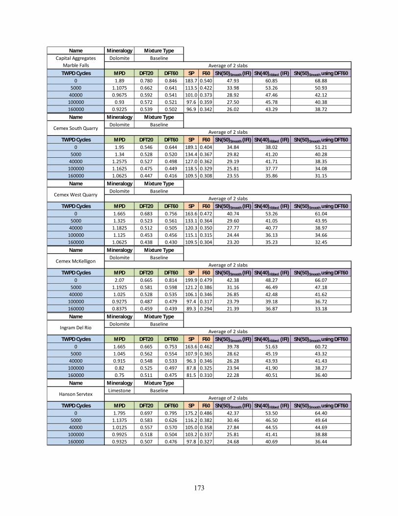
173

Name MineralogyDolomite

TWPD Cycles MPD DFT20 DFT60 SP F60 SN(50)Smooth (IFI) SN(40)ribbed (IFI) SN(50)Smooth using DFT600 1.89 0.780 0.846 183.7 0.540 47.93 60.85 68.88

5000 1.1075 0.662 0.641 113.5 0.422 33.98 53.26 50.9340000 0.9675 0.592 0.541 101.0 0.373 28.92 47.46 42.12100000 0.93 0.572 0.521 97.6 0.359 27.50 45.78 40.38160000 0.9225 0.539 0.502 96.9 0.342 26.02 43.29 38.72

Mixture TypeCapital Aggregates

Marble FallsBaseline

Average of 2 slabs

Name MineralogyDolomite

TWPD Cycles MPD DFT20 DFT60 SP F60 SN(50)Smooth (IFI) SN(40)ribbed (IFI) SN(50)Smooth using DFT600 1.95 0.546 0.644 189.1 0.404 34.84 38.02 51.21

5000 1.34 0.528 0.520 134.4 0.367 29.82 41.20 40.2840000 1.2575 0.527 0.498 127.0 0.362 29.19 41.71 38.35100000 1.1625 0.475 0.449 118.5 0.329 25.81 37.77 34.08160000 1.0625 0.447 0.416 109.5 0.308 23.55 35.86 31.15

Mixture Type

Cemex South QuarryBaseline

Average of 2 slabs

Name MineralogyDolomite

TWPD Cycles MPD DFT20 DFT60 SP F60 SN(50)Smooth (IFI) SN(40)ribbed (IFI) SN(50)Smooth using DFT600 1.665 0.683 0.756 163.6 0.472 40.74 53.26 61.04

5000 1.325 0.523 0.561 133.1 0.364 29.60 41.05 43.9540000 1.1825 0.512 0.505 120.3 0.350 27.77 40.77 38.97

100000 1.125 0.453 0.456 115.1 0.315 24.44 36.13 34.66160000 1.0625 0.438 0.430 109.5 0.304 23.20 35.23 32.45

Mixture Type

Cemex West QuarryBaseline

Average of 2 slabs

Name MineralogyDolomite

TWPD Cycles MPD DFT20 DFT60 SP F60 SN(50)Smooth (IFI) SN(40)ribbed (IFI) SN(50)Smooth using DFT600 2.07 0.665 0.814 199.9 0.479 42.38 48.27 66.07

5000 1.1925 0.581 0.598 121.2 0.386 31.16 46.49 47.1840000 1.025 0.528 0.535 106.1 0.346 26.85 42.48 41.62100000 0.9275 0.487 0.479 97.4 0.317 23.79 39.18 36.72160000 0.8375 0.459 0.439 89.3 0.294 21.39 36.87 33.18

Mixture Type

Cemex McKelligonBaseline

Average of 2 slabs

Name MineralogyDolomite

TWPD Cycles MPD DFT20 DFT60 SP F60 SN(50)Smooth (IFI) SN(40)ribbed (IFI) SN(50)Smooth using DFT600 1.665 0.665 0.753 163.6 0.462 39.78 51.63 60.72

5000 1.045 0.562 0.554 107.9 0.365 28.62 45.19 43.3240000 0.915 0.548 0.533 96.3 0.346 26.28 43.93 41.43100000 0.82 0.525 0.497 87.8 0.325 23.94 41.90 38.27160000 0.75 0.511 0.475 81.5 0.310 22.28 40.51 36.40

Mixture Type

Ingram Del RioBaseline

Average of 2 slabs

Name MineralogyLimestone

TWPD Cycles MPD DFT20 DFT60 SP F60 SN(50)Smooth (IFI) SN(40)ribbed (IFI) SN(50)Smooth using DFT600 1.795 0.697 0.795 175.2 0.486 42.37 53.50 64.40

5000 1.1375 0.583 0.626 116.2 0.382 30.46 46.50 49.6440000 1.0125 0.557 0.570 105.0 0.358 27.84 44.55 44.69100000 0.9925 0.518 0.504 103.2 0.337 25.81 41.41 38.88160000 0.9325 0.507 0.476 97.8 0.327 24.68 40.69 36.44

Mixture Type

Hanson ServtexBaseline

Average of 2 slabs

174

Name MineralogyLimestone

TWPD Cycles MPD DFT20 DFT60 SP F60 SN(50)Smooth (IFI) SN(40)ribbed (IFI) SN(50)Smooth using DFT600 1.76 0.726 0.736 172.1 0.503 43.99 56.78 59.27

5000 0.905 0.585 0.573 95.4 0.363 27.70 46.72 44.9640000 0.775 0.470 0.418 83.7 0.293 20.94 37.51 31.38100000 0.7825 0.449 0.378 84.4 0.285 20.28 36.08 27.82160000 0.785 0.423 0.372 84.6 0.273 19.27 34.18 27.29

Mixture Type

Texas Crushed StoneBaseline

Average of 2 slabs

Name MineralogyLimestone

TWPD Cycles MPD DFT20 DFT60 SP F60 SN(50)Smooth (IFI) SN(40)ribbed (IFI) SN(50)Smooth using DFT600 1.9375 0.597 0.676 188.0 0.432 37.38 42.57 54.02

5000 1.3075 0.534 0.524 131.5 0.369 29.92 41.98 40.6840000 1.1775 0.497 0.460 119.8 0.341 26.90 39.40 35.04100000 1.065 0.459 0.437 109.7 0.314 24.08 36.77 33.01160000 1.0325 0.434 0.422 106.8 0.299 22.67 34.93 31.69

Mixture Type

TXI BridgeportBaseline

Average of 2 slabs

Name MineralogyLimestone

TWPD Cycles MPD DFT20 DFT60 SP F60 SN(50)Smooth (IFI) SN(40)ribbed (IFI) SN(50)Smooth using DFT600 1.3725 0.565 0.585 137.3 0.390 32.13 44.43 46.01

5000 0.785 0.483 0.431 84.6 0.299 21.51 38.34 32.5140000 0.58 0.459 0.423 66.2 0.265 17.43 35.60 31.80100000 0.5625 0.436 0.387 64.7 0.253 16.37 33.98 28.68160000 0.555 0.419 0.367 64.0 0.245 15.70 32.87 26.89

Mixture Type

Hanson Perch HillBaseline

Average of 2 slabs

Name MineralogyLimestone

TWPD Cycles MPD DFT20 DFT60 SP F60 SN(50)Smooth (IFI) SN(40)ribbed (IFI) SN(50)Smooth using DFT600 1.56 0.701 0.783 154.1 0.477 40.85 55.52 63.42

5000 1.085 0.558 0.584 111.5 0.366 28.91 44.82 45.9340000 0.91 0.561 0.526 95.8 0.350 26.63 44.70 40.86100000 0.71 0.493 0.451 77.9 0.297 20.93 38.98 34.26160000 0.675 0.431 0.399 74.7 0.266 18.15 34.60 29.68

Mixture Type

Cemex BalconesBaseline

Average of 2 slabs

Name MineralogyLimestone

TWPD Cycles MPD DFT20 DFT60 SP F60 SN(50)Smooth (IFI) SN(40)ribbed (IFI) SN(50)Smooth using DFT600 1.47 0.694 0.766 146.1 0.467 39.62 55.26 61.86

5000 0.8325 0.510 0.510 88.9 0.319 23.54 40.85 39.4140000 0.795 0.518 0.481 85.5 0.319 23.29 41.29 36.93100000 0.76 0.456 0.416 82.4 0.286 20.34 36.68 31.23160000 0.67 0.434 0.398 74.3 0.266 18.17 34.76 29.64

Mixture TypeMartin Marietta

BeckmanBaseline

Average of 2 slabs

Name MineralogyLimestone

TWPD Cycles MPD DFT20 DFT60 SP F60 SN(50)Smooth (IFI) SN(40)ribbed (IFI) SN(50)Smooth using DFT600 1.615 0.686 0.776 159.1 0.471 40.46 53.79 62.76

5000 0.9875 0.541 0.557 102.8 0.349 26.90 43.42 43.5340000 0.885 0.511 0.504 93.6 0.325 24.32 41.07 38.89100000 0.82 0.479 0.446 87.8 0.303 22.10 38.53 33.85160000 0.75 0.448 0.401 81.5 0.281 19.88 36.05 29.88

Mixture Type

Alamo Evans RoadBaseline

Average of 2 slabs

175

Name MineralogyLimestone

TWPD Cycles MPD DFT20 DFT60 SP F60 SN(50)Smooth (IFI) SN(40)ribbed (IFI) SN(50)Smooth using DFT600 1.07 0.684 0.722 110.2 0.429 34.52 55.03 58.04

5000 0.775 0.649 0.575 83.7 0.376 28.00 50.46 45.1640000 0.595 0.578 0.542 67.6 0.315 21.61 43.26 42.27100000 0.53 0.468 0.446 61.7 0.260 16.66 35.42 33.85160000 0.5025 0.439 0.399 59.3 0.245 15.28 33.42 29.66

Mixture Type

Colorado HunterBaseline

Average of 2 slabs

Name MineralogyLimestone

TWPD Cycles MPD DFT20 DFT60 SP F60 SN(50)Smooth (IFI) SN(40)ribbed (IFI) SN(50)Smooth using DFT600 1.325 0.764 0.793 133.1 0.495 41.73 61.90 64.25

5000 0.8375 0.567 0.550 89.3 0.346 25.86 44.99 42.9540000 0.72 0.539 0.516 78.8 0.318 22.70 42.07 40.00100000 0.7125 0.463 0.447 78.1 0.284 19.87 36.93 33.89160000 0.69 0.432 0.421 76.1 0.268 18.41 34.72 31.66

Mixture Type

Ingram HondoBaseline

Average of 2 slabs

Name MineralogyLimestone

TWPD Cycles MPD DFT20 DFT60 SP F60 SN(50)Smooth (IFI) SN(40)ribbed (IFI) SN(50)Smooth using DFT600 1.955 0.637 0.754 189.6 0.458 40.01 46.53 60.84

5000 1.2575 0.523 0.557 127.0 0.359 28.87 41.20 43.5240000 1.1825 0.508 0.515 120.3 0.346 27.44 40.26 39.86100000 1.0775 0.451 0.452 110.9 0.310 23.82 36.05 34.37160000 1.0075 0.433 0.422 104.6 0.297 22.37 34.92 31.74

Mixture TypeMartin Marietta

CenterpointBaseline

Average of 2 slabs

Name MineralogyLimestone

TWPD Cycles MPD DFT20 DFT60 SP F60 SN(50)Smooth (IFI) SN(40)ribbed (IFI) SN(50)Smooth using DFT600 1.2775 0.790 0.828 128.8 0.504 42.34 64.03 67.33

5000 0.845 0.585 0.547 90.0 0.355 26.69 46.32 42.6540000 0.75 0.550 0.532 81.5 0.327 23.64 43.08 41.35100000 0.7175 0.478 0.445 78.6 0.290 20.41 37.85 33.71160000 0.71 0.424 0.388 77.9 0.265 18.29 34.07 28.74

Mixture TypeMartin Marietta New

BraunfelsBaseline

Average of 2 slabs

Limestone

TWPD Cycles MPD DFT20 DFT60 SP F60 SN(50)Smooth (IFI) SN(40)ribbed (IFI) SN(50)Smooth using DFT600 1.6125 0.774 0.828 158.8 0.521 45.21 61.83 67.33

5000 1.16 0.595 0.620 118.3 0.391 31.48 47.72 49.0740000 1.0325 0.563 0.553 106.8 0.364 28.47 45.21 43.25100000 0.9 0.536 0.521 94.9 0.338 25.57 42.99 40.38160000 0.8875 0.465 0.448 93.8 0.303 22.39 37.54 34.04

Mummie MummieBaseline

Average of 2 slabs

Name MineralogyLimestone

TWPD Cycles MPD DFT20 DFT60 SP F60 SN(50)Smooth (IFI) SN(40)ribbed (IFI) SN(50)Smooth using DFT600 1.6775 0.699 0.779 164.7 0.482 41.73 54.67 63.00

5000 0.9 0.560 0.569 94.9 0.350 26.55 44.77 44.6240000 0.7825 0.579 0.561 84.4 0.345 25.42 45.53 43.94100000 0.745 0.518 0.474 81.0 0.312 22.38 40.85 36.32160000 0.72 0.493 0.461 78.8 0.298 21.04 38.95 35.17

Mixture TypeSouth West Aggregate

(SWA) KnippaBaseline

Average of 2 slabs

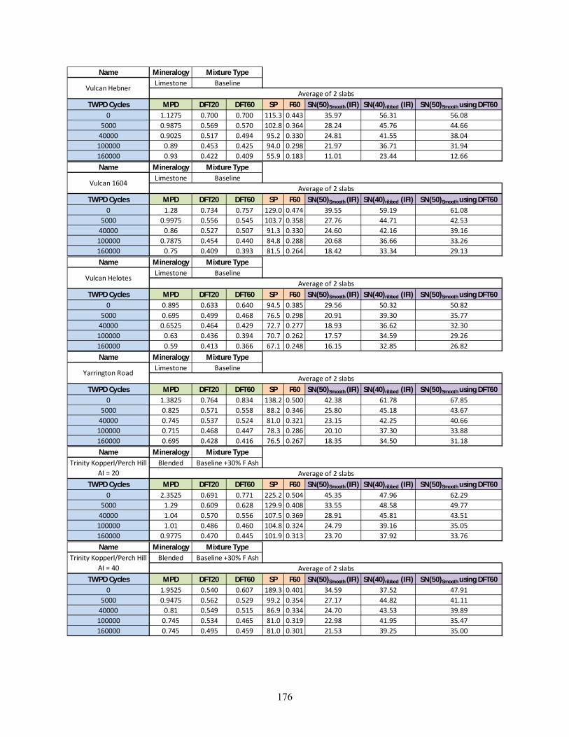
176

Name MineralogyLimestone

TWPD Cycles MPD DFT20 DFT60 SP F60 SN(50)Smooth (IFI) SN(40)ribbed (IFI) SN(50)Smooth using DFT600 1.1275 0.700 0.700 115.3 0.443 35.97 56.31 56.08

5000 0.9875 0.569 0.570 102.8 0.364 28.24 45.76 44.6640000 0.9025 0.517 0.494 95.2 0.330 24.81 41.55 38.04100000 0.89 0.453 0.425 94.0 0.298 21.97 36.71 31.94160000 0.93 0.422 0.409 55.9 0.183 11.01 23.44 12.66

Mixture Type

Vulcan HebnerBaseline

Average of 2 slabs

Name MineralogyLimestone

TWPD Cycles MPD DFT20 DFT60 SP F60 SN(50)Smooth (IFI) SN(40)ribbed (IFI) SN(50)Smooth using DFT600 1.28 0.734 0.757 129.0 0.474 39.55 59.19 61.08

5000 0.9975 0.556 0.545 103.7 0.358 27.76 44.71 42.5340000 0.86 0.527 0.507 91.3 0.330 24.60 42.16 39.16100000 0.7875 0.454 0.440 84.8 0.288 20.68 36.66 33.26160000 0.75 0.409 0.393 81.5 0.264 18.42 33.34 29.13

Mixture Type

Vulcan 1604Baseline

Average of 2 slabs

Name MineralogyLimestone

TWPD Cycles MPD DFT20 DFT60 SP F60 SN(50)Smooth (IFI) SN(40)ribbed (IFI) SN(50)Smooth using DFT600 0.895 0.633 0.640 94.5 0.385 29.56 50.32 50.82

5000 0.695 0.499 0.468 76.5 0.298 20.91 39.30 35.7740000 0.6525 0.464 0.429 72.7 0.277 18.93 36.62 32.30100000 0.63 0.436 0.394 70.7 0.262 17.57 34.59 29.26160000 0.59 0.413 0.366 67.1 0.248 16.15 32.85 26.82

Mixture Type

Vulcan HelotesBaseline

Average of 2 slabs

Name MineralogyLimestone

TWPD Cycles MPD DFT20 DFT60 SP F60 SN(50)Smooth (IFI) SN(40)ribbed (IFI) SN(50)Smooth using DFT600 1.3825 0.764 0.834 138.2 0.500 42.38 61.78 67.85

5000 0.825 0.571 0.558 88.2 0.346 25.80 45.18 43.6740000 0.745 0.537 0.524 81.0 0.321 23.15 42.25 40.66100000 0.715 0.468 0.447 78.3 0.286 20.10 37.30 33.88160000 0.695 0.428 0.416 76.5 0.267 18.35 34.50 31.18

Mixture Type

Yarrington RoadBaseline

Average of 2 slabs

Name MineralogyBlended

TWPD Cycles MPD DFT20 DFT60 SP F60 SN(50)Smooth (IFI) SN(40)ribbed (IFI) SN(50)Smooth using DFT600 2.3525 0.691 0.771 225.2 0.504 45.35 47.96 62.29

5000 1.29 0.609 0.628 129.9 0.408 33.55 48.58 49.7740000 1.04 0.570 0.556 107.5 0.369 28.91 45.81 43.51100000 1.01 0.486 0.460 104.8 0.324 24.79 39.16 35.05160000 0.9775 0.470 0.445 101.9 0.313 23.70 37.92 33.76

Mixture TypeTrinity Kopperl/Perch Hill

AI = 20Baseline +30% F Ash

Average of 2 slabs

Name MineralogyBlended

TWPD Cycles MPD DFT20 DFT60 SP F60 SN(50)Smooth (IFI) SN(40)ribbed (IFI) SN(50)Smooth using DFT600 1.9525 0.540 0.607 189.3 0.401 34.59 37.52 47.91

5000 0.9475 0.562 0.529 99.2 0.354 27.17 44.82 41.1140000 0.81 0.549 0.515 86.9 0.334 24.70 43.53 39.89100000 0.745 0.534 0.465 81.0 0.319 22.98 41.95 35.47160000 0.745 0.495 0.459 81.0 0.301 21.53 39.25 35.00

Mixture TypeTrinity Kopperl/Perch Hill

AI = 40Baseline +30% F Ash

Average of 2 slabs

177

Name MineralogyBlended

TWPD Cycles MPD DFT20 DFT60 SP F60 SN(50)Smooth (IFI) SN(40)ribbed (IFI) SN(50)Smooth using DFT600 2.025 0.713 0.792 195.8 0.507 44.94 53.34 64.21

5000 0.93 0.590 0.586 97.6 0.368 28.27 47.16 46.1140000 0.6925 0.582 0.553 76.3 0.332 23.72 44.67 43.25100000 0.6725 0.553 0.502 74.5 0.317 22.31 42.54 38.73160000 0.66 0.528 0.479 73.4 0.304 21.13 40.66 36.75

Mixture TypeTrinity Kopperl/Perch Hill

AI = 60Baseline +30% F Ash

Average of 2 slabs

Name MineralogyBlended

TWPD Cycles MPD DFT20 DFT60 SP F60 SN(50)Smooth (IFI) SN(40)ribbed (IFI) SN(50)Smooth using DFT600 1.925 0.770 0.724 186.9 0.535 47.43 59.41 58.17

5000 1.07 0.582 0.570 110.2 0.377 29.85 46.80 44.7440000 0.95 0.547 0.506 99.4 0.349 26.70 43.89 39.06100000 0.875 0.500 0.464 92.7 0.319 23.75 40.26 35.39160000 0.8575 0.490 0.457 91.1 0.312 23.09 39.48 34.77

Mixture TypeTXI Paradise/TXI

Bridgeport AI = 20Baseline +30% F Ash

Average of 2 slabs

Name MineralogyBlended

TWPD Cycles MPD DFT20 DFT60 SP F60 SN(50)Smooth (IFI) SN(40)ribbed (IFI) SN(50)Smooth using DFT600 2.04 0.763 0.755 197.2 0.537 47.89 57.96 60.96

5000 1.1625 0.588 0.587 118.5 0.388 31.21 47.18 46.2040000 0.97 0.556 0.507 101.2 0.355 27.33 44.58 39.17100000 0.95 0.521 0.487 99.4 0.336 25.57 41.88 37.46160000 0.945 0.502 0.469 99.0 0.326 24.69 40.42 35.83

Mixture TypeTXI Paradise/TXI

Bridgeport AI = 40Baseline +30% F Ash

Average of 2 slabs

Name MineralogyBlended

TWPD Cycles MPD DFT20 DFT60 SP F60 SN(50)Smooth (IFI) SN(40)ribbed (IFI) SN(50)Smooth using DFT600 2.14 0.768 0.860 206.2 0.544 48.85 57.63 70.14

5000 1.1075 0.621 0.613 113.5 0.401 32.10 49.95 48.5040000 0.895 0.587 0.530 94.5 0.360 27.38 46.47 41.22100000 0.8875 0.549 0.498 93.8 0.342 25.73 43.63 38.43160000 0.8825 0.535 0.490 93.4 0.335 25.08 42.58 37.68

Mixture TypeTXI Paradise/TXI

Bridgeport AI = 60Baseline +30% F Ash

Average of 2 slabs

178

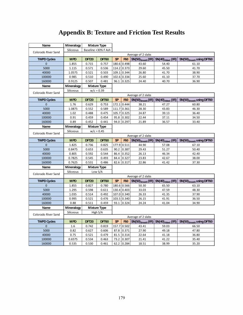
179

Appendix B: Texture and Friction Test Results

Name MineralogySiliceous

TWPD Cycles MPD DFT20 DFT60 SP F60 SN(50)Smooth (IFI) SN(40)ribbed (IFI) SN(50)Smooth using DFT600 1.855 0.715 0.757 180.6 0.498 43.60 54.40 61.10

5000 1.115 0.571 0.536 114.2 0.373 29.60 45.50 41.7040000 1.0575 0.521 0.503 109.1 0.344 26.80 41.70 38.90100000 0.985 0.510 0.490 102.6 0.334 25.60 41.10 37.70160000 0.9125 0.507 0.481 96.1 0.325 24.40 40.70 36.90

Mixture Type

Colorado River SandBaseline +30% F Ash

Average of 2 slabs

Name MineralogySiliceous

TWPD Cycles MPD DFT20 DFT60 SP F60 SN(50)Smooth (IFI) SN(40)ribbed (IFI) SN(50)Smooth using DFT600 1.76 0.629 0.753 172.1 0.444 38.21 47.27 60.80

5000 1.0875 0.552 0.589 111.7 0.361 28.30 43.83 46.3040000 1.02 0.488 0.475 105.7 0.325 24.87 39.13 36.40100000 0.91 0.459 0.454 95.8 0.302 22.44 37.11 34.50160000 0.89 0.452 0.441 94.0 0.297 21.89 36.57 33.40

Mixture Type

Colorado River Sandw/c = 0.39

Average of 2 slabs

Name MineralogySiliceous

TWPD Cycles MPD DFT20 DFT60 SP F60 SN(50)Smooth (IFI) SN(40)ribbed (IFI) SN(50)Smooth using DFT600 1.825 0.736 0.825 177.9 0.511 44.90 57.08 67.10

5000 0.8475 0.653 0.635 90.2 0.387 29.43 51.27 50.4040000 0.805 0.592 0.544 86.4 0.352 26.13 46.34 42.40100000 0.7825 0.545 0.493 84.4 0.327 23.83 42.67 38.00160000 0.7625 0.531 0.486 82.6 0.317 22.86 41.42 37.30

Mixture Type

Colorado River Sandw/c = 0.45

Average of 2 slabs

Name MineralogySiliceous

TWPD Cycles MPD DFT20 DFT60 SP F60 SN(50)Smooth (IFI) SN(40)ribbed (IFI) SN(50)Smooth using DFT600 1.855 0.827 0.780 180.6 0.566 50.30 65.50 63.10

5000 1.295 0.598 0.611 130.4 0.403 33.03 47.59 48.3040000 1.035 0.514 0.492 107.0 0.340 26.33 41.35 37.90100000 0.995 0.521 0.476 103.5 0.340 26.15 41.91 36.50160000 0.88 0.511 0.459 93.1 0.324 24.24 41.04 34.90

Mixture Type

Colorado River SandLow S/A

Average of 2 slabs

Name MineralogySiliceous

TWPD Cycles MPD DFT20 DFT60 SP F60 SN(50)Smooth (IFI) SN(40)ribbed (IFI) SN(50)Smooth using DFT600 1.6 0.742 0.819 157.7 0.502 43.41 59.03 66.50

5000 0.82 0.627 0.606 87.8 0.371 27.90 49.18 47.8040000 0.75 0.521 0.479 81.5 0.314 22.64 41.18 36.80100000 0.6575 0.534 0.463 73.2 0.307 21.41 41.22 35.40160000 0.535 0.530 0.461 62.2 0.284 18.51 38.99 35.20

Mixture Type

Colorado River SandHigh S/A

Average of 2 slabs

180

Name MineralogySiliceous

TWPD Cycles MPD DFT20 DFT60 SP F60 SN(50)Smooth (IFI) SN(40)ribbed (IFI) SN(50)Smooth using DFT600 1.095 0.675 0.669 112.4 0.427 34.45 54.34 53.40

5000 0.77 0.560 0.535 83.3 0.334 24.47 44.08 41.6040000 0.7625 0.560 0.486 82.6 0.333 24.33 44.01 37.30100000 0.74 0.534 0.461 80.6 0.319 22.98 42.06 35.20160000 0.6725 0.546 0.474 74.5 0.314 22.11 42.16 36.30

Mixture Type

Colorado River SandLow Paste

Average of 2 slabs

Name MineralogySiliceous

TWPD Cycles MPD DFT20 DFT60 SP F60 SN(50)Smooth (IFI) SN(40)ribbed (IFI) SN(50)Smooth using DFT600 1.955 0.642 0.725 189.6 0.462 40.47 47.23 58.30

5000 1.1275 0.578 0.592 115.3 0.379 30.18 46.19 46.6040000 0.9875 0.590 0.556 102.8 0.372 28.89 47.02 43.40100000 0.915 0.542 0.499 96.3 0.342 25.92 43.32 38.50160000 0.85 0.542 0.499 90.4 0.334 24.80 42.86 38.50

Mixture Type

Colorado River SandHigh Paste

Average of 2 slabs

Name MineralogyLimestone

TWPD Cycles MPD DFT20 DFT60 SP F60 SN(50)Smooth (IFI) SN(40)ribbed (IFI) SN(50)Smooth using DFT600 1.23 0.667 0.766 124.5 0.430 35.20 52.90 61.90

5000 0.81 0.635 0.583 86.9 0.370 27.60 49.10 45.9040000 0.6025 0.507 0.449 68.2 0.287 19.40 38.80 34.10100000 0.57 0.448 0.400 65.3 0.258 16.90 34.70 29.80160000 0.5575 0.422 0.379 64.2 0.247 15.80 33.10 28.00

Mixture Type

Hanson Perch Hillw/c = 0.39

Average of 2 slabs

Name MineralogyLimestone

TWPD Cycles MPD DFT20 DFT60 SP F60 SN(50)Smooth (IFI) SN(40)ribbed (IFI) SN(50)Smooth using DFT600 1.575 0.758 0.800 155.5 0.510 44.10 60.70 64.90

5000 1.045 0.611 0.615 107.9 0.390 30.80 49.10 48.6040000 0.96 0.515 0.479 100.3 0.334 25.50 41.50 36.70100000 0.93 0.431 0.411 97.6 0.290 21.50 35.00 30.70160000 0.835 0.429 0.406 89.1 0.282 20.30 34.90 30.30

Mixture Type

Hanson Perch Hillw/c = 0.45

Average of 2 slabs

Name MineralogyLimestone

TWPD Cycles MPD DFT20 DFT60 SP F60 SN(50)Smooth (IFI) SN(40)ribbed (IFI) SN(50)Smooth using DFT600 1.4475 0.731 0.753 144.0 0.486 41.39 58.73 60.70

5000 0.985 0.573 0.510 102.6 0.364 28.26 45.89 39.4040000 0.925 0.488 0.458 97.2 0.318 23.89 39.40 34.90100000 0.92 0.460 0.431 96.7 0.304 22.62 37.22 32.50160000 0.8575 0.439 0.409 91.1 0.288 20.97 35.63 30.60

Mixture Type

TXI BridgeportBaseline +30% F Ash

Average of 2 slabs

Name MineralogyLimestone

TWPD Cycles MPD DFT20 DFT60 SP F60 SN(50)Smooth (IFI) SN(40)ribbed (IFI) SN(50)Smooth using DFT600 0.985 0.654 0.629 102.6 0.405 31.90 52.30 49.90

5000 0.7175 0.610 0.521 78.6 0.349 25.30 47.00 40.4040000 0.6825 0.541 0.453 75.4 0.313 22.10 41.80 34.40100000 0.6425 0.516 0.434 71.8 0.297 20.40 39.70 32.80160000 0.585 0.496 0.414 66.7 0.279 18.60 37.80 31.00

Mixture Type

TXI BridgeportLow S/A

Average of 2 slabs

181

Name MineralogyLimestone

TWPD Cycles MPD DFT20 DFT60 SP F60 SN(50)Smooth (IFI) SN(40)ribbed (IFI) SN(50)Smooth using DFT600 1.595 0.672 0.718 157.3 0.461 39.50 52.50 57.70

5000 1.04 0.621 0.604 107.5 0.393 31.00 49.60 47.7040000 1.01 0.610 0.562 104.8 0.384 30.10 48.60 44.00100000 0.91 0.480 0.437 95.8 0.312 23.30 38.60 33.10160000 0.81 0.462 0.421 86.9 0.294 21.30 37.30 31.70

Mixture Type

TXI BridgeportHigh S/A

Average of 2 slabs

Name MineralogyLimestone

TWPD Cycles MPD DFT20 DFT60 SP F60 SN(50)Smooth (IFI) SN(40)ribbed (IFI) SN(50)Smooth using DFT600 2.785 0.545 0.694 264.0 0.424 37.90 28.18 55.60

5000 1.6275 0.575 0.651 160.2 0.409 34.59 43.63 51.8040000 1.3725 0.560 0.554 137.3 0.387 31.88 44.01 43.30100000 1.3025 0.456 0.468 131.0 0.327 26.09 35.45 35.80160000 1.27 0.430 0.433 128.1 0.311 24.53 33.40 32.70

Mixture Type

TXI BridgeportLow Paste

Average of 2 slabs

Name MineralogyLimestone

TWPD Cycles MPD DFT20 DFT60 SP F60 SN(50)Smooth (IFI) SN(40)ribbed (IFI) SN(50)Smooth using DFT600 1.5325 0.683 0.750 151.7 0.463 39.45 53.79 60.50

5000 0.805 0.623 0.598 86.4 0.368 27.52 48.83 47.2040000 0.7275 0.556 0.521 79.5 0.327 23.54 43.40 40.40100000 0.6525 0.487 0.443 72.7 0.287 19.72 38.14 33.60160000 0.625 0.460 0.429 70.3 0.271 18.29 36.10 32.30

Mixture Type

TXI BridgeportHigh Paste

Average of 2 slabs

Name MineralogyDolomite

TWPD Cycles MPD DFT20 DFT60 SP F60 SN(50)Smooth (IFI) SN(40)ribbed (IFI) SN(50)Smooth using DFT600 1.5275 0.796 0.789 151.2 0.527 45.50 64.10 63.90

5000 0.7925 0.658 0.614 85.3 0.382 28.70 51.30 48.6040000 0.7725 0.626 0.563 83.5 0.365 27.10 48.80 44.10100000 0.7125 0.545 0.486 78.1 0.320 22.90 42.50 37.30160000 0.6675 0.530 0.469 74.1 0.307 21.48 41.07 35.80

Mixture TypeCapital Aggregates

Marble FallsBaseline +30% F Ash

Average of 2 slabs

Name MineralogyDolomite

TWPD Cycles MPD DFT20 DFT60 SP F60 SN(50)Smooth (IFI) SN(40)ribbed (IFI) SN(50)Smooth using DFT600 1.5525 0.663 0.729 153.5 0.455 38.77 52.14 58.70

5000 1.11 0.611 0.624 113.8 0.396 31.70 49.10 49.5040000 1.0625 0.502 0.477 109.5 0.336 26.10 40.40 36.50100000 0.9725 0.535 0.518 101.4 0.345 26.50 43.00 40.10160000 0.9125 0.497 0.473 96.1 0.321 24.10 40.10 36.20

Mixture TypeCapital Aggregates

Marble Fallsw/c = 0.39

Average of 2 slabs

Name MineralogyDolomite

TWPD Cycles MPD DFT20 DFT60 SP F60 SN(50)Smooth (IFI) SN(40)ribbed (IFI) SN(50)Smooth using DFT600 1.5025 0.705 0.779 149.0 0.474 40.30 55.84 63.00

5000 0.9525 0.647 0.660 99.6 0.398 31.07 51.66 52.6040000 0.825 0.560 0.534 88.2 0.341 25.37 44.40 41.60100000 0.795 0.531 0.501 85.5 0.325 23.79 42.20 38.60160000 0.7425 0.569 0.515 80.8 0.334 24.28 44.42 39.90

Mixture TypeCapital Aggregates

Marble Fallsw/c = 0.45

Average of 2 slabs

182

Name MineralogySlate

TWPD Cycles MPD DFT20 DFT60 SP F60 SN(50)Smooth (IFI) SN(40)ribbed (IFI) SN(50)Smooth using DFT600 1.43 0.580 0.632 142.5 0.400 33.14 45.10 50.12

5000 0.915 0.614 0.559 96.3 0.376 28.89 48.68 43.7540000 0.91 0.535 0.471 95.8 0.337 25.45 42.59 36.00100000 0.835 0.530 0.486 89.1 0.327 24.21 42.07 37.36160000 0.775 0.492 0.455 83.7 0.301 21.52 38.64 34.60

Mixture Type

Lattimore StringtownBaseline +30% F Ash

Average of 2 slabs

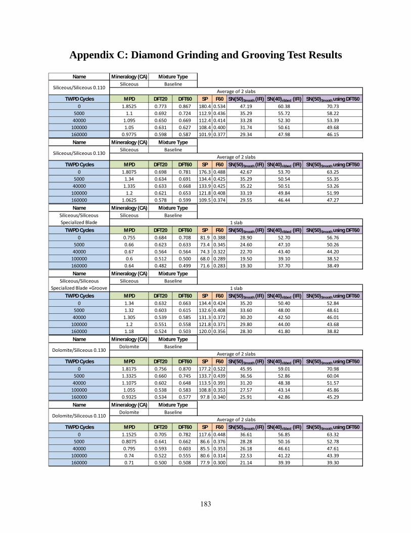
183

Appendix C: Diamond Grinding and Grooving Test Results

Name Mineralogy (CA)Siliceous

TWPD Cycles MPD DFT20 DFT60 SP F60 SN(50)Smooth (IFI) SN(40)ribbed (IFI) SN(50)Smooth using DFT600 1.8525 0.773 0.867 180.4 0.534 47.19 60.38 70.73

5000 1.1 0.692 0.724 112.9 0.436 35.29 55.72 58.2240000 1.095 0.650 0.669 112.4 0.414 33.28 52.30 53.39

100000 1.05 0.631 0.627 108.4 0.400 31.74 50.61 49.68160000 0.9775 0.598 0.587 101.9 0.377 29.34 47.98 46.15

Siliceous/Siliceous 0.110Baseline

Average of 2 slabs

Mixture Type

Name Mineralogy (CA)Siliceous

TWPD Cycles MPD DFT20 DFT60 SP F60 SN(50)Smooth (IFI) SN(40)ribbed (IFI) SN(50)Smooth using DFT600 1.8075 0.698 0.781 176.3 0.488 42.67 53.70 63.25

5000 1.34 0.634 0.691 134.4 0.425 35.29 50.54 55.3540000 1.335 0.633 0.668 133.9 0.425 35.22 50.51 53.26

100000 1.2 0.621 0.653 121.8 0.408 33.19 49.84 51.99160000 1.0625 0.578 0.599 109.5 0.374 29.55 46.44 47.27

Average of 2 slabs

Mixture Type

Siliceous/Siliceous 0.130Baseline

Name Mineralogy (CA)Siliceous

TWPD Cycles MPD DFT20 DFT60 SP F60 SN(50)Smooth (IFI) SN(40)ribbed (IFI) SN(50)Smooth using DFT600 0.755 0.684 0.708 81.9 0.388 28.90 52.70 56.76

5000 0.66 0.623 0.633 73.4 0.345 24.60 47.10 50.2640000 0.67 0.564 0.564 74.3 0.322 22.70 43.40 44.20

100000 0.6 0.512 0.500 68.0 0.289 19.50 39.10 38.52160000 0.64 0.482 0.499 71.6 0.283 19.30 37.70 38.49

Siliceous/Siliceous Specialized Blade

Baseline1 slab

Mixture Type

Name Mineralogy (CA)Siliceous

TWPD Cycles MPD DFT20 DFT60 SP F60 SN(50)Smooth (IFI) SN(40)ribbed (IFI) SN(50)Smooth using DFT600 1.34 0.632 0.663 134.4 0.424 35.20 50.40 52.84

5000 1.32 0.603 0.615 132.6 0.408 33.60 48.00 48.6140000 1.305 0.539 0.585 131.3 0.372 30.20 42.50 46.01

100000 1.2 0.551 0.558 121.8 0.371 29.80 44.00 43.68160000 1.18 0.524 0.503 120.0 0.356 28.30 41.80 38.82

1 slab

Mixture TypeSiliceous/Siliceous

Specialized Blade +GrooveBaseline

Name Mineralogy (CA)Dolomite

TWPD Cycles MPD DFT20 DFT60 SP F60 SN(50)Smooth (IFI) SN(40)ribbed (IFI) SN(50)Smooth using DFT600 1.8175 0.756 0.870 177.2 0.522 45.95 59.01 70.98

5000 1.3325 0.660 0.745 133.7 0.439 36.56 52.86 60.0440000 1.1075 0.602 0.648 113.5 0.391 31.20 48.38 51.57

100000 1.055 0.538 0.583 108.8 0.353 27.57 43.14 45.86160000 0.9325 0.534 0.577 97.8 0.340 25.91 42.86 45.29

Dolomite/Siliceous 0.130Baseline

Average of 2 slabs

Mixture Type

Name Mineralogy (CA)Dolomite

TWPD Cycles MPD DFT20 DFT60 SP F60 SN(50)Smooth (IFI) SN(40)ribbed (IFI) SN(50)Smooth using DFT600 1.1525 0.705 0.782 117.6 0.448 36.61 56.85 63.32

5000 0.8075 0.641 0.662 86.6 0.376 28.28 50.16 52.7840000 0.795 0.593 0.603 85.5 0.353 26.18 46.61 47.61

100000 0.74 0.522 0.555 80.6 0.314 22.53 41.22 43.39160000 0.71 0.500 0.508 77.9 0.300 21.14 39.39 39.30

Dolomite/Siliceous 0.110Baseline

Average of 2 slabs

Mixture Type

184

Name Mineralogy (CA)Dolomite

TWPD Cycles MPD DFT20 DFT60 SP F60 SN(50)Smooth (IFI) SN(40)ribbed (IFI) SN(50)Smooth using DFT600 0.715 0.656 0.705 78.3 0.369 27.00 50.20 56.52

5000 0.705 0.594 0.614 77.4 0.340 24.50 45.80 48.5340000 0.655 0.572 0.590 73.0 0.323 22.70 43.70 46.45

100000 0.6 0.503 0.519 68.0 0.285 19.20 38.60 40.26160000 0.58 0.466 0.486 66.2 0.267 17.60 36.00 37.34

1 slab

Mixture TypeDolomite/Siliceous Specialized Blade

Baseline

Name Mineralogy (CA)Dolomite

TWPD Cycles MPD DFT20 DFT60 SP F60 SN(50)Smooth (IFI) SN(40)ribbed (IFI) SN(50)Smooth using DFT600 1.645 0.636 0.648 161.8 0.444 38.00 49.10 51.54

5000 1.595 0.566 0.594 157.3 0.402 33.90 43.10 46.8240000 1.66 0.516 0.533 163.1 0.377 31.60 38.00 41.41

100000 1.59 0.502 0.507 156.8 0.366 30.40 37.30 39.14160000 1.57 0.478 0.505 155.0 0.352 29.00 35.30 38.96

Dolomite/Siliceous Specialized Blade +Groove

Baseline1 slab

Mixture Type

Name Mineralogy (CA)Limestone

TWPD Cycles MPD DFT20 DFT60 SP F60 SN(50)Smooth (IFI) SN(40)ribbed (IFI) SN(50)Smooth using DFT600 1.76 0.693 0.800 172.1 0.483 42.02 53.53 64.83

5000 1.0875 0.556 0.629 111.7 0.366 28.87 44.69 49.8540000 1.0125 0.464 0.504 105.0 0.313 23.85 37.43 38.87

100000 0.9525 0.429 0.475 99.6 0.291 21.66 34.80 36.32160000 0.9025 0.438 0.475 95.2 0.292 21.50 35.59 36.32

TXI B/Siliceous 0.130Baseline

Average of 2 slabs

Mixture Type

Name Mineralogy (CA)Limestone

TWPD Cycles MPD DFT20 DFT60 SP F60 SN(50)Smooth (IFI) SN(40)ribbed (IFI) SN(50)Smooth using DFT600 1.79 0.744 0.861 174.8 0.514 45.10 58.10 70.22

5000 1.105 0.608 0.637 113.3 0.393 31.44 48.85 50.5540000 0.8125 0.527 0.566 87.1 0.324 23.85 41.93 44.31

100000 0.7825 0.494 0.519 84.4 0.306 22.13 39.46 40.26160000 0.7225 0.470 0.477 79.0 0.288 20.29 37.46 36.57

Average of 2 slabs

Mixture Type

TXI B/Siliceous 0.110Baseline

Name Mineralogy (CA)Limestone

TWPD Cycles MPD DFT20 DFT60 SP F60 SN(50)Smooth (IFI) SN(40)ribbed (IFI) SN(50)Smooth using DFT600 0.725 0.551 0.557 79.2 0.324 23.30 43.10 43.56

5000 0.665 0.506 0.540 73.9 0.296 20.60 39.50 42.1140000 0.62 0.463 0.489 69.8 0.272 18.30 36.30 37.56

100000 0.605 0.409 0.442 68.5 0.248 16.30 32.70 33.48160000 0.59 0.432 0.428 67.1 0.255 16.70 34.00 32.25

TXI B/Siliceous Specialized Blade

Baseline1 slab

Mixture Type

Name Mineralogy (CA)Limestone

TWPD Cycles MPD DFT20 DFT60 SP F60 SN(50)Smooth (IFI) SN(40)ribbed (IFI) SN(50)Smooth using DFT600 1.68 0.542 0.552 164.9 0.393 33.20 40.20 43.16

5000 1.61 0.542 0.539 158.6 0.389 32.70 40.80 42.0140000 1.5 0.495 0.504 148.8 0.358 29.50 37.40 38.92

100000 1.49 0.405 0.419 147.9 0.307 24.70 29.40 31.49160000 1.47 0.402 0.415 146.1 0.305 24.40 29.30 31.14

TXI B/Siliceous Specialized Blade +Groove

Baseline1 slab

Mixture Type

185

Name Mineralogy (CA)Limestone

TWPD Cycles MPD DFT20 DFT60 SP F60 SN(50)Smooth (IFI) SN(40)ribbed (IFI) SN(50)Smooth using DFT600 1.475 0.660 0.761 146.5 0.448 37.88 52.21 61.47

5000 1.1225 0.603 0.646 114.9 0.392 31.43 48.44 51.3840000 0.97 0.523 0.552 101.2 0.339 25.95 42.08 43.13

100000 0.9475 0.483 0.508 99.2 0.317 23.95 39.01 39.27160000 0.9025 0.428 0.457 95.2 0.287 21.08 34.82 34.81

Average of 2 slabs

Mixture Type

TXI B/TXI B 0.130Baseline

Name Mineralogy (CA)Limestone

TWPD Cycles MPD DFT20 DFT60 SP F60 SN(50)Smooth (IFI) SN(40)ribbed (IFI) SN(50)Smooth using DFT600 1.455 0.672 0.760 144.7 0.454 38.43 53.52 61.36

5000 0.96 0.580 0.612 100.3 0.365 28.13 46.26 48.3540000 1.005 0.488 0.507 104.3 0.325 24.85 39.36 39.21

100000 0.8325 0.395 0.435 88.9 0.265 18.82 32.27 32.83160000 0.77 0.417 0.433 83.3 0.269 18.94 33.87 32.64

TXI B/TXI B 0.110Baseline

Average of 2 slabs

Mixture Type

Name Mineralogy (CA)Limestone

TWPD Cycles MPD DFT20 DFT60 SP F60 SN(50)Smooth (IFI) SN(40)ribbed (IFI) SN(50)Smooth using DFT600 0.75 0.600 0.684 81.5 0.350 25.60 46.70 54.70

5000 0.79 0.572 0.533 85.1 0.343 25.30 45.10 41.4440000 0.69 0.465 0.478 76.1 0.282 19.60 36.90 36.60

100000 0.685 0.460 0.482 75.6 0.279 19.30 36.60 36.96160000 0.65 0.419 0.433 72.5 0.258 17.30 33.60 32.72

TXI B/TXI B Specialized Blade

Baseline1 slab

Mixture Type

Name Mineralogy (CA)Limestone

TWPD Cycles MPD DFT20 DFT60 SP F60 SN(50)Smooth (IFI) SN(40)ribbed (IFI) SN(50)Smooth using DFT600 1.675 0.620 0.673 164.4 0.437 37.40 47.40 53.74

5000 1.55 0.570 0.570 153.2 0.403 33.80 43.80 44.6840000 1.46 0.476 0.486 145.2 0.345 28.20 36.00 37.30

100000 1.42 0.424 0.477 141.6 0.315 25.20 31.70 36.52160000 1.4 0.412 0.424 139.8 0.308 24.50 30.90 31.90

1 slab

Mixture TypeTXI B/TXI B Specialized

Blade +GrooveBaseline

Name Mineralogy (CA)Limestone

TWPD Cycles MPD DFT20 DFT60 SP F60 SN(50)Smooth (IFI) SN(40)ribbed (IFI) SN(50)Smooth using DFT600 1.74 0.731 0.825 170.3 0.504 43.97 57.21 67.07

5000 1.1875 0.657 0.704 120.7 0.425 34.63 52.68 56.4440000 1.0775 0.524 0.546 110.9 0.348 27.18 41.97 42.58

100000 0.945 0.459 0.482 99.0 0.305 22.84 37.09 36.99160000 0.8275 0.395 0.402 88.4 0.265 18.87 32.45 29.97

Perch Hill/Perch Hill 0.130Baseline

Average of 2 slabs

Mixture Type

Name Mineralogy (CA)Limestone

TWPD Cycles MPD DFT20 DFT60 SP F60 SN(50)Smooth (IFI) SN(40)ribbed (IFI) SN(50)Smooth using DFT600 1.3775 0.633 0.691 137.8 0.425 35.23 49.82 55.34

5000 0.9175 0.561 0.595 96.5 0.352 26.88 44.96 46.8640000 0.785 0.487 0.518 84.6 0.303 21.86 38.92 40.14

100000 0.795 0.431 0.466 85.5 0.278 19.80 34.90 35.59160000 0.7825 0.426 0.433 84.4 0.274 19.42 34.49 32.68

Perch Hill/Perch Hill 0.110Baseline

Average of 2 slabs

Mixture Type

186

Name Mineralogy (CA)Limestone

TWPD Cycles MPD DFT20 DFT60 SP F60 SN(50)Smooth (IFI) SN(40)ribbed (IFI) SN(50)Smooth using DFT600 0.815 0.506 0.532 87.3 0.315 23.10 40.50 41.34

5000 0.71 0.494 0.515 77.9 0.297 21.00 39.10 39.8840000 0.65 0.438 0.461 72.5 0.266 18.00 34.90 35.17

100000 0.64 0.423 0.427 71.6 0.258 17.30 33.80 32.16160000 0.62 0.398 0.420 69.8 0.245 16.20 32.10 31.55

Perch Hill/Perch Hill Specialized Blade

Baseline1 slab

Mixture Type

Name Mineralogy (CA)Limestone

TWPD Cycles MPD DFT20 DFT60 SP F60 SN(50)Smooth (IFI) SN(40)ribbed (IFI) SN(50)Smooth using DFT600 1.83 0.503 0.543 178.4 0.375 31.80 35.20 42.34

5000 1.53 0.540 0.550 151.4 0.384 32.00 41.20 42.9640000 1.46 0.460 0.505 145.2 0.336 27.40 34.60 39.04

100000 1.685 0.395 0.444 165.3 0.308 25.10 26.60 33.68160000 1.435 0.377 0.396 142.9 0.290 22.90 27.50 29.46

Perch Hill/Perch Hill Specialized Blade +Groove

Baseline1 slab

Mixture Type