use of unmanned aerial vehicles (uav) for urban tree

Clemson UniversityTigerPrints

All Theses Theses

8-2014

USE OF UNMANNED AERIAL VEHICLES(UAV) FOR URBAN TREE INVENTORIESBrian RitterClemson University, [email protected]

Follow this and additional works at: https://tigerprints.clemson.edu/all_theses

Part of the Forest Sciences Commons, Geographic Information Sciences Commons, and theNatural Resources Management and Policy Commons

This Thesis is brought to you for free and open access by the Theses at TigerPrints. It has been accepted for inclusion in All Theses by an authorizedadministrator of TigerPrints. For more information, please contact [email protected].

Recommended CitationRitter, Brian, "USE OF UNMANNED AERIAL VEHICLES (UAV) FOR URBAN TREE INVENTORIES" (2014). All Theses. 1890.https://tigerprints.clemson.edu/all_theses/1890

https://tigerprints.clemson.edu?utm_source=tigerprints.clemson.edu%2Fall_theses%2F1890&utm_medium=PDF&utm_campaign=PDFCoverPages

https://tigerprints.clemson.edu/all_theses?utm_source=tigerprints.clemson.edu%2Fall_theses%2F1890&utm_medium=PDF&utm_campaign=PDFCoverPages

https://tigerprints.clemson.edu/theses?utm_source=tigerprints.clemson.edu%2Fall_theses%2F1890&utm_medium=PDF&utm_campaign=PDFCoverPages

https://tigerprints.clemson.edu/all_theses?utm_source=tigerprints.clemson.edu%2Fall_theses%2F1890&utm_medium=PDF&utm_campaign=PDFCoverPages

http://network.bepress.com/hgg/discipline/90?utm_source=tigerprints.clemson.edu%2Fall_theses%2F1890&utm_medium=PDF&utm_campaign=PDFCoverPages



https://tigerprints.clemson.edu/all_theses/1890?utm_source=tigerprints.clemson.edu%2Fall_theses%2F1890&utm_medium=PDF&utm_campaign=PDFCoverPages

mailto:[email protected]

USE OF UNMANNED AERIAL VEHICLES (UAV) FOR

URBAN TREE INVENTORIES

____________________________________________________________________

A Thesis

Presented to

The Graduate School of

Clemson University

____________________________________________________________________

In Partial Fulfillment

of the Requirements for the Degree

Master of Science

Forest Resources

by

Brian A. Ritter

August 2014

Accepted by:

Dr. Christopher J. Post, Committee Chair

Dr. Elena Mikhailova

Dr. Larry Gering

ii

ABSTRACT

In contrast to standard aerial imagery, unmanned aerial systems (UAS) utilize recent

technological advances to provide an affordable alternative for imagery acquisition.

Increased value can be realized through clarity and detail providing higher resolution (2-5

cm) over traditional products. Many natural resource disciplines such as urban forestry

will benefit from UAS. Tree inventories for risk assessment, biodiversity, planning, and

design can be efficiently achieved with the UAS. Recent advances in photogrammetric

processing have proved automated methods for three dimensional rendering of aerial

imagery. Point clouds can be generated from images providing additional benefits.

Association of spatial locational information within the point cloud can be used to

produce elevation models i.e. digital elevation, digital terrain and digital surface. Taking

advantage of this point cloud data, additional information such as tree heights can be

obtained. Several software applications have been developed for LiDAR data which can

be adapted to utilize UAS point clouds. This study examines solutions to provide tree

inventory and heights from UAS imagery. Imagery taken with a micro-UAS was

processed to produce a seamless orthorectified image. This image provided an accurate

way to obtain a tree inventory within the study boundary. Utilizing several methods, tree

height models were developed with variations in spatial accuracy. Model parameters

were modified to offset spatial inconsistencies providing statistical equality of means.

Statistical results (p = 0.756) with a level of significance (α = 0.01) between measured

iii

and modeled tree height means resulted with 82% of tree species obtaining accurate tree

heights. Within this study, the UAS has proven to be an efficient tool for urban forestry

providing a cost effective and reliable system to obtain remotely sensed data.

Keywords: Aerial Photography, Arboriculture, Clemson University, GIS, LiDAR,

Remote Sensing, Tree Height, Tree Inventory, UAVS, UAV

iv

DEDICATION

This study is dedicated to my wife Laurie and son Zachary. They have supported me

throughout my time at Clemson and they deserve a large amount of credit, for they have

provided beyond measure patience, support and love to help me succeed.

v

ACKNOWLEDGEMENTS

I wish to thank my committee: Dr. Christopher Post, Committee Chairman, Dr. Elena

Mikhailova, and Dr. Lawrence Gering for their help and support during development and

completion of this study. Thanks to Clemson University Facilities Services for

providing funding, and to Paul Minerva, Clemson University Arborist, for insight and

support. I acknowledge and thank Russell Buchanan, GIS Specialist, for providing field

work, photogrammetry assistance and data entry. Technical Contribution No. 6162 of the

Clemson University Experiment Station.

vi

TABLE OF CONTENTS

Page

TITLE PAGE ....................................................................................................................... i

ABSTRACT ........................................................................................................................ ii

DEDICATION ................................................................................................................... iv

ACKNOLWLEDGMENTS .................................................................................................v

LIST OF FIGURES ......................................................................................................... viii

LIST OF TABLES ............................................................................................................. ix

CHAPTER

I INTRODUCTION .............................................................................................1

II MATERIALS AND METHODS .......................................................................8

Study Area ................................................................................................8

UAV Aerial Imagery ................................................................................8

Imagery Processing ...................................................................................8

Tree Inventory...........................................................................................9

Field Analysis ...........................................................................................9

Generation of DEM, DTM, and CHM ......................................................9

Calculate Tree Heights............................................................................11

Statistical Analysis ..................................................................................11

III RESULTS AND DISCUSSION ......................................................................12

UAV Imagery ..........................................................................................12

Imagery Processing .................................................................................12

Tree Inventory .........................................................................................15

Field Analysis ..........................................................................................15

Generation of DEM, DTM, and CHM ....................................................16

Calculate Tree Heights ............................................................................21

Statistical Analysis ..................................................................................22

vii

Table of Contents (Continued)

IV CONCLUSION.................................................................................................25

V APPENDIX .......................................................................................................51

Glossary ...................................................................................................51

Flow Diagram for LASTool Processing .................................................56

REFERENCES ..................................................................................................................57

viii

LIST OF FIGURES

Figure Page

1 General classification of UAV’s ................................................................................26

2 LiDAR returns when laser pulses hit the ground and trees .......................................27

3 Study boundary where UAV will be implemented ....................................................28

4 Ground control station during launch of UAV ..........................................................29

5 Ground control software during actual UAV mission ...............................................30

6 Example of tonal imbalances and spatial alignment inaccuracies occurring after

image processing .........................................................................................31

7 Completed orthomosaic of study boundary created from UAV images ....................32

8 Results of tree inventory created on orthomosaic from UAV images .......................33

9 Screen capture of tree inventory attribute table after field data was added ...............34

10 Spatial comparison of Dronemapper point cloud and tree inventory point ..............35

11 TiFFS output using LiDAR point cloud with tree inventory points .........................36

12 TiFFS output using UAV point cloud with tree inventory points ............................37

13 Fusion canopy height model results with tree inventory points ...............................38

14 Screen capture of tree inventory attribute table with interpolated elevations

from UAV point cloud DEM and DTM models .........................................39

ix

LIST OF TABLES

Table Page

1 Unmanned aerial vehicle (UAV) products related to urban forest uses ....................40

2 Benefits of having a tree inventory ............................................................................41

3 American Society of Photogrammetry and Remote Sensing (ASPRS) standard

LiDAR point classes ...................................................................................42

4 Aerial coverage by UAV flights in summer 2013 .....................................................43

5 Comparative analysis between UAV and field tree inventory techniques for

summer 2013 flight mission .......................................................................44

6 Flow design for processing UAV point cloud using LASTools to classify points

and create DTM and DEM ..........................................................................45

7 Statistical results comparing measured and estimated tree heights based on tree

inventory location to closest LiDAR point .................................................46

8 Statistical comparison of grass and building values to develop a scale factor for

pixel conversion to actual elevation heights ...............................................47

9 Statistical results of comparing measured and estimated tree heights using

Agisoft/LASTool point cloud analysis interpolated to tree inventory

points ...........................................................................................................48

10 Statistical comparison of means for individual tree species that have measured

and estimated tree heights ...........................................................................49

1

CHAPTER 1

INTRODUCTION

Unmanned aerial vehicles (UAV) or unmanned aircraft vehicle systems (UAVS) have

in recent years, established their presence across the world even though they have been

around since the 1920’s (Arjomandi, 2007). Comprising 93% of aerial reconnaissance

during World War I, balloons were the forerunner of the modern day UAV (Blom, 2010).

Primarily developed for the military, advancement in technologies has lead to increased

UAV applications within natural resource disciplines. Monitoring, surveillance, mapping

and three dimensional (3D) modeling are the primarily natural resource UAV

applications. Little of the potential has been realized in civilian UAV applications

(Merino et.al. 2006). In the United States, existing/unclear regulatory restrictions

governing UAV/UAVS use has limited commercial use. Within natural resource

disciplines, research is ongoing and new opportunities are rapidly emerging as the

technology advancements continue. Despite the regularity uncertainty, UAV use is

showing extensive value within natural resources and agriculture communities.

The UAV is an aircraft that can be controlled from the ground maintaining a level

flight pattern in the absence of an onboard pilot (Elias, 2012). There are many different

designs for UAV air frames which fall into two general categories; fixed and rotary

winged (Figure 1) (Elias, 2012; DIY, 2013). With varying design in body and wing type

general classifications can be further divided by performance parameters which include:

weight, payload, longevity, range, motor type, maximum altitude and speed (Remondino

et. al. 2011). Additionally alternate characteristics for classification can include: cost and

2

wing span (Arjomandi, 2007). Autonomous, air, hand and mechanical launch methods

vary with size and type of UAV. The UAV size limits the type of application and sensor

carried onboard. Sensor development within consumer digital camera markets has seen

many technological advances resulting in much smaller, affordable and effective sensors

for smaller UAV platforms. Technological advances in digital cameras, geographical

positioning systems (GPS), and autopilots allowed the use of smaller UAV’s as platforms

for remote sensing. Autopilots with onboard GPS aid in flight control, positioning of data

being collected and even landing, resulting in ease of use and autonomous flight. Data

collected while in flight can be directly stored on the aircraft or sent in real time back to

ground control station (DIY, 2013)

Sensors on UAV’s can produce an array of remotely sensed products. True color

UAV orthophotography results in imagery with higher resolution (2 – 3 cm) and detail

compared to traditional aerial imagery. Hyperspectral or multi-spectral imagery can be

acquired from onboard UAV sensors. (Johnston et. al, 2003) Near Infrared (NIR) filters

can be used to modify standard digital camera sensors resulting in vegetative monitoring

products (Hunt, et. al, 2010). Thermal sensors allow for detecting temperature changes

across the landscape (Rudol and Doherty, 2008). Development efforts are ongoing to

fit Light Detection and Ranging (LIDAR) sensors on smaller UAV’s (Wallace, 2012). In

addition, full motion videos with real time data acquisition are possible using current

technologies (Eugster and Nebiker, 2008).

UAV applications are in their infancy, however many applications are beginning to

emerge. Vegetative health monitoring, precision agriculture, urban forestry, emergency

3

management, biological and traffic monitoring represent current application areas for the

UAVs. Once legislative and regulatory factors in the United States are clarified, civilian

applications of UAV’s will become more prevalent. Modern UAV systems provide; low

cost, high resolution imagery, currency of information, repeatability, short turnaround

processing, mobility, reliability and an ease of use system (Laliberte et. al. 2008, Rango

and Laliberte, 2010).

National Air Space (NAS) in the United States is governed by the Federal Aviation

Administration (FAA). Civilian and commercial UAV’s are limited in their application

until new FAA rules can be developed. A detailed look at regulation and control of UAV

use has begun due to increased civilian and commercial interests. In 2006, the FAA

produced a document, “Unmanned Aircraft Operations in the National Airspace System”,

to detail special considerations towards use of a UAV within government, police,

emergency management and university research. This is limiting the commercial/civilian

growth of the UAV in the United States not only from its use but through research and

development as companies are reluctant to move forward with regulatory uncertainty.

Congress has increased the FAA budget to include funds to develop a UAV program. In

February 2012, an appropriation was signed by President Obama and with financial

support included mandates to streamline permits for UAV use and rule development

(Mitchell, 2012). The FAA Modernization and Reform Act of 2012; details the

requirements for the FAA to integrate UAV into the NAS by fiscal year 2015. In July

2012, the FAA released a fact sheet detailing its current stance on commercial use. The

primary concern of FAA is focused on safety and they are considering the need for

4

integrated sense and avoid technology in UAV’s. Privacy, national security, and GPS

signal interference have factored into the decision by the FAA to limit UAV civilian and

commercial applications. (GAO, 2012)

In natural resources, the urban forest is well suited for small UAV applications. UAV

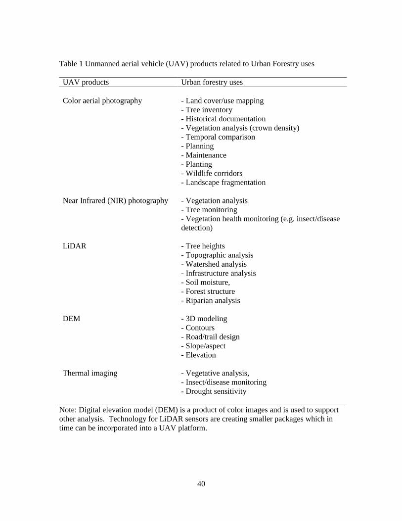
generated products for urban forestry can be used in many ways (Table 1). Urban forest

management objectives are dictated by human use of the areas around trees. To

understand how people use the urban forest and to determine tree diversity, it is important

to create a spatial tree inventory. Tree diversity across the landscape can be identified

with accurate inventories that detail forest characteristics (Rowntree, 1988). An indirect

benefit of inventory analysis with the UAV is the collection and archive of aerial imagery

for future temporal comparison. The affordable repeatability of acquiring UAV imagery

offers the opportunity to complete spatiotemporal analysis to detect change over time.

Remotely sensed data is ideal for detecting urban forest spatial patterns to map this

change (Jomaa et. al, 2008). Traditional aerial photography methods may be limited in

this respect because of the high cost of obtaining repeated imagery. Multi-temporal data

can be collected by the UAV that will provide effective comparisons to provide

understanding in landscape change and monitoring (Zhou and Wang, 2011). Inventory

and spatial comparisons will provide valuable information of urban forest structure,

diversity, and management. This information will lead to more effective management

decisions.

Urban forest management begins with a tree inventory. Tree inventories provide

information as to tree diversity, location, condition, size and species. They also provide

5

positive benefits to communities and jurisdictions (Table 2). Tree inventories are an

essential component of developing an urban forest management plan. Inventories

represent urban forest conditions at the time of data collection. Urban forests are

dynamic with natural and man-made changes occurring often and inventories require

updating on a regular basis. There are several ways to develop tree inventories with each

having its own set of advantages and disadvantages. Economic considerations may

dictate which methods are used for obtaining a tree inventory (NCFS, 2014).

Urban forest inventories have data collected depending on the primary motivation for

the inventory. Typically, standard information that is collected from each tree includes:

species, diameter, condition, maintenance needs, location (x, y coordinate) and growing

conditions (canopy, soil type/volume, and moisture regimes) (NCFS, 2014). As part of

an urban tree inventory, tree risk assessment is typically included. Management of tree

risk is designed to mitigate both basic and complex urban infrastructure to identify

potential for tree failure. Urban forest managers have the responsibility to identify

varying tree risk levels present and to manage them in accordance to acceptable risk.

Tree risk involves inspection and assessment of the risk trees pose to property or human

injury (Pokorny et. al, 2003). Tree risk assessment can be divided into three levels; Level

1- limited visual inspection, Level 2- complete visual inspection, and Level 3- advanced

assessment (ISA, 2013). Tree risk identifies the potential for failure and environmental

conditions contributing to failure along with target analysis. In the urban forest, tree

failure could result in significant damage to human health and property. (Ellison, 2005)

6

Light Detection and Ranging (LiDAR) uses light pulsed from a laser to measure

distance to the earth’s surface (Figure 2). Highly accurate three dimensional information

regarding the earth’s surface and objects on the surface can be obtained from LiDAR

information (NOAA, 2013). Forest inventory, urban planning, landscape ecology,

floodplain mapping, hydrologic modeling, geomorphology are some of the examples of

how LiDAR data is being utilized (Chen, 2007). Using LiDAR has key advantages: it

can be quickly collected, provides high sample density, collected in dense forest,

collected day or night, and contains no geometric distortion (ESRI, 2014). A limiting

factor to temporal acquisition of LiDAR is high acquisition cost (Chen, 2007). LiDAR

data can be processed to determine vertical canopy structure and individual tree 3D

modeling (Wang et. al, 2008). LiDAR data is in the form of a point cloud and when

classified can produce results in the form of digital terrain models (DTM), digital

elevation models (DEM) and canopy height models (CHM) (Yunfei et. al, 2008, ESRI,

2014). The Log ASCII Standard (LAS) file format is used to interchange LiDAR data

between users. This file type is binary and maintains specific LiDAR characteristics

while reducing complexity found in generic ASCII file structure. The LAS format is

flexible to allow for customization within specific applications using an LAS Domain

Profile (ASPRS, 2012). Each point in the LiDAR data set is classified to define object

types encountered by laser pulses. Using classification codes (LAS 1.1 or LAS 1.2 or

LAS 1.3) standardization is achieved to define classification values (Table 3).

Delineation of ground and high vegetation points can be converted to raster data to

determine tree heights using tools within ArcGIS software (ESRI, 2014). In contrast to

7

traditional LiDAR data acquisition, UAV generated imagery can be processed using

multi-view stereopsis, to produce a point cloud similar to LiDAR. These point clouds

can be processed using LiDAR methods resulting in DEM, DTM, and CHM products.

(Harwin and Lucieer, 2012)

It is hypothesized that UAV products (imagery and 3D point cloud) can be used in

place of traditional data to obtain tree inventories and heights. Objectives of this study

are to: 1) evaluate the efficacy of a small UAV for routine urban aerial photo acquisitions

in urban forestry, 2) produce spatially-referenced aerial photo orthomosics from a UAV,

3) produce a tree inventory from UAV imagery, 4) use 3D point cloud from UAV

imagery to develop a model that will accurately produce tree height values.

8

CHAPTER 2

MATERIALS AND METHODS

Study Area

Clemson University lies in the southwest corner of Pickens County in northwest South

Carolina. This land grant university was founded in 1889 from a private gift of Thomas

Clemson and was formally opened in 1893. Today the main campus covers 566 ha with

an additional 12,949 ha of agriculture and forest land (Clemson, 2013). The purchase of

a single winged vehicle called the SwingletCam (Figure 1) was acquired to aid in campus

planning, and tree inventory. On the campus of Clemson University, deployment of a

UAV occurred in October 2012. This study will be conducted across the main campus

located in Clemson, SC (Figure 3).

UAV Aerial Imagery

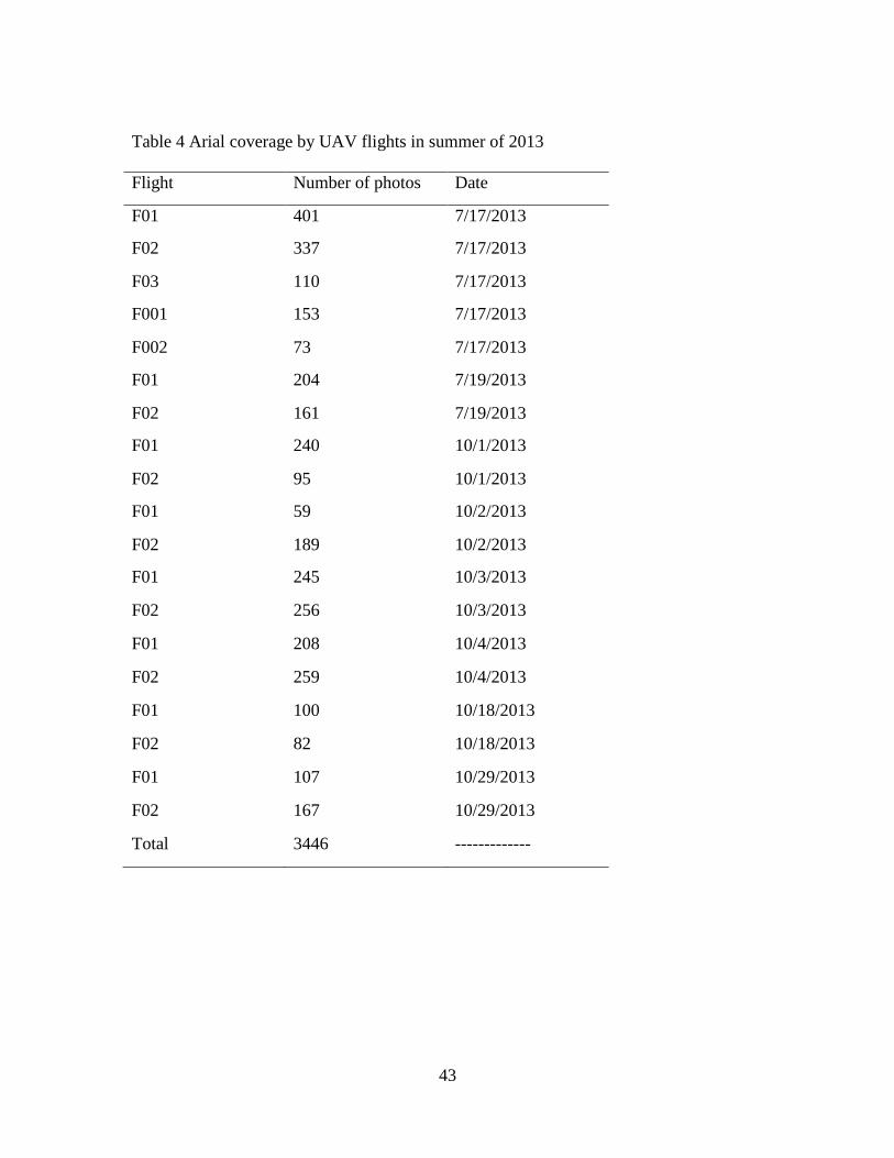
Multiple missions were conducted between July and October 2013 (Table 4) to

evaluate operational procedures and acquisition of aerial images. Missions were planned

using strategic landing/take off zones to make efficient use of topography and

photographic parameters. Geodetic ground control points (115) were established using

geographic positioning system (GPS) to aid spatial referencing of images. Results were

analyzed to evaluate altitude preferences, radio connectivity, image resolution/detail, and

flight parameters.

Imagery Processing

Imagery was transferred from the UAV storage media to a computer for orthophoto

processing. Images were geotagged with flight log data and processed to produce a

9

seamless orthorectified image for the study boundary. Open source, third party

applications, and cloud based services were used to evaluate effectiveness in producing a

seamless image derived from multiple temporal missions.

Tree Inventory

A tree inventory was conducted using the orthorectified images. A feature class

representing the tree inventory was created based on UAV imagery using ArcGIS 10.1

software (ESRI, 2010). A heads up digitizing technique records tree locations as points

through visual inspection of the high-resolution imagery. Each point corresponds to a

single tree added in a feature class representing the overall tree inventory. Using pre-

identified tree maintenance zones, the tree inventory process was conducted along a

gridded pattern until each zone was complete. This process meets the requirement for

Level 1 tree risk assessment.

Field Analysis

Field visits were conducted at each tree identified within the tree inventory. Species,

diameter at breast height (DBH), and total tree height data was obtained. DBH was

measured with a Biltmore stick (Black, 2014) and a Nikon Forestry Pro Model 8381 laser

range finder ( 0.31 m) was used to obtain total tree heights. During field visits, visible

defects were noted and recorded using a gps-enabled digital camera. The field analysis

represents a level 2 tree risk assessment.

Generation of DEM, DTM, and CHM

Using LiDAR and UAV 3D point cloud data, a DEM, DTM, and CHM were

generated. LiDAR data was used as a base line to validate UAV point cloud results.

10

Processing of both data sets was conducted using different approaches. Raw LiDAR data

in LAS format were processed using the Fusion LIDAR viewing and analysis software

developed by the United States Forest Service (USFS) to produce 3D terrain and canopy

surface models (USFS, 2014). A Toolbox for LiDAR Data Filtering and Forest Studies

(TiFFS) analyzes LiDAR LAS data processing them into terrain raster files (object height

models (OHM), DEM, DSM), GIS feature classes (tree points, tree canopy polygons) and

statistical raster files (kurtosis height, mean height, percent height, quad mean height,

skewness height, standard deviation height). TiFFS utilize an automated routine that does

not require pre-classified LIDAR point clouds for input. Having a more focused

approach to obtaining forest information from LiDAR, TiFFS is designed to extract

specific statistical related information in addition to terrain modeling (Globalidar, 2014).

Among many tools that ArcGIS contains, LiDAR LAS files can be utilized to obtain

terrain models. Additional toolsets can be used to analyze the terrain models and extract

information such as tree heights. Using the UAV point cloud data may require additional

software to prepare it for use. Converting the point cloud into LAS or ASCII format for

input is typically required. There are products such as Microsoft Excel and Structured

Query Language (SQL) Database for example, that can accomplish this conversion but

due to the number of table rows (tens of millions for each mission) there may be

limitations encountered due to large file sizes. Martin Isenburg has produced a set of

tools (LASTools) specifically for LAS management (Rapidlasso, 2014). These tools can

be used in a standalone graphical user interface, as a toolbox in ArcGIS or executed

within operating system command line. This toolbox allows for quick and efficient

11

conversion of UAV point cloud data into LAS format. Agisoft is commercial based

software that can process UAV images into a seamless orthorectified product. A single

orthomosaic seamless image along with a 3D point cloud can be produced with Agisoft to

develop a tree inventory and tree height model.

Calculate Tree Heights

Canopy Height Models (CHM) and object height models (OHM) derived from point

cloud analysis can be used to directly obtain tree heights. Spatial interpolation at each

tree location was used to extract these values to the tree inventory attribute table. ArcGIS

10.1 was used to spatially join this information to the point location files. Utilizing other

tools in ArcGIS 10.1 (LASTools), the elevation models were developed and elevation

values spatially joined to tree inventory points. These values were subtracted to obtain

estimated tree heights.

Statistical Analysis

Statistical comparison of tree heights to field measured heights was conducted.

Hypothesis testing of two means was used to validate the tree height model. If the null

hypotheses are not rejected then the conclusion will show the means are equal and

validate the tree height model. In the case of rejecting the null hypothesis, further

statistical analysis was conducted to determine what factors may contribute to the

rejection. Results can reveal if some tree species may not be subject to tree height

modeling or other factors may cause spatial inconstancies or inaccurate elevation values

limiting accurate interpolated values to be obtained.

12

CHAPTER 3

RESULTS AND DISCUSSION

UAV Imagery

Nineteen UAV flights were flown between July and October 2013 (Table 4). A

portable ground control station (Figure 4) was used to manage flight control with

Emotion2 software (Figure 5). A total of 3466 color images with resolutions of 2.6-3.6

cm were collected from a typical altitude of 90 m. Between each image, 60% side lap

and 40% forward lap parameters were used. This was needed to minimize distortional

balances between images. The resolution obtained is useful to provide the scale needed

to describe forest canopy and diversity variables within the forested landscape (Anderson

and Gaston, 2013). During flight, images were stored on a secure digital (SD) card.

Flight functions were provided with an onboard autopilot and GPS. Autonomous take off

and landings provided ease of use. Ground control communication with the UAV was

maintained using a 2.4 GHz radio link via a universal serial bus (USB) computer

connection. The UAV functioned flawless at low altitudes and provided an effective

solution for obtaining high resolution aerial photography.

Imagery Processing

Processing of images began with geotagging flight and camera information to each

image. Geotagging was completed using a proprietary software (Post Flight Suite)

supplied with the UAV. Geotagging adds information to the EXIF header that contains

camera parameters and spatial x, y coordinate. A cloud based service (DroneMapper,

http://dronemapper.com) was used to orthorectify and mosaic flights into a seamless

http://dronemapper.com/

13

image. Only 2497 of the 3466 images were used for mosaic processing. Some images

were dropped as they represented extended overlap between flights. In between flights

with varying temporal periods introduced tonal imbalances, excessive shading (sun angle

differences) and color inconsistencies. The extra images allowed for a selection process

to choose the best image for orthorectification and minimization of potential visual

inaccuracies. Prior to uploading flight images, ground control information was created

using a GCP application supplied by DroneMapper. Two text files were needed to allow

for georeferencing images to ground control. A file containing the name, x coordinate, y

coordinate, z value and horizontal/vertical precision for each ground control point was

used as a ground reference file (3D file). With DroneMapper’s proprietary GCP

software, images were analyzed to determine if any ground control was present. If

present, the ground control point was selected with the computer mouse which correlated

to the x, y pixel value on the image. A separate file (2D file) stored the name, x pixel,

and y pixel values. The 2D file was edited changing the name to match its corresponding

ground control point name. After all images were examined, both text files containing

the ground control (3D file) and image control (2D file) information was uploaded with

flight images. Due to the large number of images sent for processing, Dronemapper

divided the image set into five processing blocks for increased efficiency. After

processing by DroneMapper, products were returned which included orthorectified

seamless image, DEM, DSM, and 3D point cloud for each block of images.

Upon receipt of DroneMapper products, each flight block was loaded into ArcGIS

10.1 for evaluation. In ArcGIS 10.1 additional mosaic tools were used to create a

14

seamless image of all flight blocks. Tonal imbalance (Figure 6) between flights occurred

and with further analysis where not completely eliminated. A spatial grid (305 m x 305

m) was developed to clip original flight images. This process allowed for areas of tonal

balance issues to be further edited by choosing flight overlaps that could be used to

replace the tonal imbalances. From the tiled images, a new mosaic (Figure 7) was

developed however tonal imbalances and color matching were not totally removed. The

results from the additional processing improved the original product making it useful to

obtain tree inventories.

Further investigation to enhance the image processing, a commercial application,

Agisoft PhotoScan Professional Edition Ver. 1.0.4 (64bit) (http://www.agisoft.ru/) was

used. Agisoft is designed to process photogrammetry data for orthorectification with

additional functionality to produce an orthomosic image, DEM, DTM and 3D point

clouds. The same 2466 images used for Dronemapper processing were used as inputs to

Agisoft creating a single orthorectified mosaic. This operation stressed computer

resources (8 core processor, 32 gb RAM) during implementation. Results were examined

in ArcGIS 10.1 and although minor tonal balances were present. Agisoft had overall

better results over DroneMapper resulting in improved spatial accuracy and tonal

balancing. Dronemapper minimized building distortion in contrast to Agisoft were

buildings were misshaped and warped. In addition, a 3D point cloud was exported from

Agisoft for utilization in tree height modeling.

http://www.agisoft.ru/

15

Tree Inventory

The high resolution characteristics of the completed mosaic enhanced visual

identification of individual trees for urban forest analysis and level 1 tree risk assessment.

Using ArcGIS 10.1, individual trees were located and assigned a unique x/y coordinate

by mouse click with the point added to the tree inventory feature class (Figure 8).

Acquisition for both field and UAV tree inventory data was timed to calculate a total time

per tree. The time per tree was multiplied by the total number of trees acquired during

data collection for each method. The results (Table 5) reflected a realized savings of 29.3

days when using UAV methods. This information is invaluable as a way to offset limited

resources for arboriculture applications.

Field Analysis

Field work is still ongoing to visit non-sampled trees. The goal is to visit all trees

identified within the tree inventory. Currently, 1831 trees have been examined for level 2

risk assessment. Species, DBH, total height, and general condition were noted. DBH

was obtained using a Biltmore stick (Black, 2014). Total tree heights were measured

using a Nikon Forestry Pro Model 8381 range finder. A three point method was used to

compute heights with the rangefinder. Ranging measurements were taken directly from

three tree positions: eye level, base, and top of tree. Internally these measurements were

used to return a tree height value. Data collected were field recorded pen and paper

method. ArcGIS 10.1 was used to edit the tree inventory feature class, keycoding field

data associated with each tree (Figure 9). A total of 57 unique tree species were

16

identified through field observations. Diversity among trees is represented by 31 genus

and 46 species.

Generation of DEM, DTM, and CHM

Generation of elevation models was conducted using Agisoft and Dronemapper

products. Models were derived utilizing TiFFS, Fusion, ArcGIS and LASTools. Each

model was evaluated for spatial and tree height accuracies.

Dronemapper supplied DEM, DTM and point cloud files. The DEM and DTM were

compared to LiDAR DEM. It was observed, pixel values for the UAV based DEM and

DTM products were not true elevation values. It was surmised that these values were

missing a scale factor to correlate with actual elevation values. In an attempt to develop a

scale factor, a point grid was developed using the LiDAR and DroneMapper DEM pixel

values. These were spatially assigned to each point in the grid. Using the field calculator

in ArcGIS 10.1, a new attribute was assigned a scale up factor derived from dividing the

LiDAR elevation by the pixel value. Points were then randomly selected and classified

into grass (open flat areas) and buildings (top of building). The means of each classified

group of points were looked at statistically to see if there were differences based on cover

type. The result was used to scale the pixel value to represent actual elevation. The

results, where successful for ground elevation (DEM) however, the scale factor was not

valid to accurately assimilate height elevations.

The point cloud provided by DroneMapper included x, y and z values for each pixel in

the mosaic imagery. Assuming the z value represents object height, the x and y values

could be used to spatially locate each pixel. Through tools in ArcGIS 10.1, a raster

17

model representing the y value could be produced. Due to extremely large (millions)

point cloud files, data preparation was necessary to use the files in ArcGIS. The X, Y

Data tool requires a text or Microsoft Excel file to spatially locate each pixel. Excel has a

1,048,000 row limit so each point cloud file had to be parsed into smaller files. Each

point cloud file can be programmatically split into manageable sizes then converted to

excel format for processing. This task did not prove to be efficient due to the number of

files produced and time needed for conversion. This method was processed at a smaller

scale for testing. One flight was processed to produce a point file that could be spatially

joined to tree inventory. Spatial inaccuracies occurred with actual tree inventory

locations not in line with x, y generated points. In an attempt to correct spatial offsets,

the near tool in ArcGIS 10.1 was used to select the closes elevation to a measured tree. It

was found that the closest point was not always the correct one. In many instances, the

correct pixel was farther away from the closest point. The neighborhood analysis (3 x 3)

tool in ArcGIS 10.1 was used to evaluate the points. This method captured in many cases

the correct pixel and the maximum value within each neighborhood could be used for tree

height interpolation (Figure 10). This process contained variability across spatial extents

and was not considered a feasible method without modification.

The LAS Toolkit (Rapidlasso, 2014) includes the txt2LAS tool. DroneMapper point

cloud files were converted without parsing of data into a file similar to LiDAR. The new

file was used to build a raster model representing the z value. A comparison was made

against the LiDAR DEM. When compared to the LiDAR DEM, resulting point cloud z

values were negative. This indicates it was representing elevations below the DEM. It

18

was concluded that the z value in DroneMapper’s point cloud did not represent object

height and were not in the same scale. More information needs to be gathered from

DroneMapper as to methods and metadata before the point cloud can be used in tree

height modeling.

Utilizing TiFFS proved to be user friendly with its automated process to take LAS

files and create estimates of forest metrics. It was designed specifically to utilize LiDAR

information to analyze forest structure. The outcome from TiFFS produced several

results: DEM, DSM, OHM, ground and object LAS point cloud, and ESRI shapefiles

representing crown, and trees. Interpolated tree height values are present in the attribute

table and can be compared with tree inventory measured heights. Both LiDAR and

DroneMapper point clouds were analyzed in TiFFS. Outcomes for both point clouds

were compared to the tree inventory both visually and statistically. Spatial comparisons

show inaccuracies in tree location for both LiDAR and UAV Dronemapper derived point

clouds (Figure 11-12). The LiDAR results have a closer spatial relationship to inventory

trees. Further investigation is needed to determine the cause for spatial inaccuracies;

however it is hypothesized that map projections and projection transformations may be

the cause of the inaccuracy.

Fusion (USFS, 2014) utilizes user developed command line files to produce canopy

(CHM) and elevation models (DEM). LiDAR point clouds were processed using this

method. CHM returned spatial correlation to tree inventory (Figure 13). Spatial

interpolation at tree locations joined CHM elevations to tree inventory points. Measured

tree heights were compared to CHM values statistically to determine equality. The

19

results were inconsistent across the tree inventory. Slight to moderate differences in tree

heights were observed.

ArcGIS 10.1 provides tools designed for processing LiDAR point clouds. These tools

were utilized to develop a DTM model. A DEM model was not needed, since one was

provided with the LiDAR point cloud. Inconsistent point cloud classifications (only

ground point’s classified-LAS 2) were used to develop a DTM from vegetative

classifications (LAS 1-first returns). The result was spatially interpolated to tree

inventory points. Using the LIDAR (3.05 m x 3.05 m) derived DEM supplied with the

LiDAR point cloud, the tree inventory revealed interpolated elevation values in like

manner. A comparison of the DEM and DTM values concluded dissimilarity between

measured and estimated tree heights. Statistical analysis was performed to determine

equality. Measured and interpolated tree heights were considered equal if pvalue < level

of significance (0.01). Statistical results concluded that inequality existed across the

study boundary. It was perceived that this result was not spatially explicit and elevation

data was subdivided into tiles for statistical analysis. A pattern of discontinuity was

found indicating that the model did represent object heights within certain spatial extents.

There seems to be some indication that map projection, datum and unit transformation

may have introduced error into the model. In addition it is hypothesized, that filtering of

unclassified points during processing could have included outliers that skewed the results.

In addition, the date of acquisition between LIDAR (2011) and UAV (2013) data could

cause dissimilarity between elevations.

20

Agisoft was used to generate a seamless orthomosaic and 3D point cloud by using

each UAV image (2497 total) in a six step process. The process aligned, built

geometries, georeferenced, meshed, textured, and mosaicked the images into a single true

color high resolution image and point cloud. The resulting image was an improvement

over other results with no tonal imbalances and spatial accuracies within 10.5 cm of

geodetic control. Some building distortion was present but did not distract from the trees.

A point cloud containing x, y, z, Red (R), Green (G), Blue (B) values for each point was

exported as a text file. LASTools was used to convert the text file into an unclassified

LiDAR (. las) format. In Agisoft, to obtain increased spatial accuracy, native UAV map

projection (WGS1984 Lat/Long) was used. To utilize LASTools, a conversion of the

map projection was required to convert the point cloud file to UTM WGS 1984 Zone

17N. Due to point cloud file size (209+ million points) tiling was used to parse the file

into smaller units for processing. Each file was batched processed (Table 6) to: tile,

classify ground points, convert z values to true heights, and classify building/high

vegetation points using default parameters built into each tool. A LASTool (las2DEM)

for creating DEM’s was used to convert the ground and high vegetation points into

separate DSM and DTM models. These tools were utilized within an application

developed in ArcGIS Model Builder to streamline LASTool utilization. A BAT file was

created to enable LASTool to process all tiles in sequence for greater efficiency using a

step value of 0.25 representing a 25 cm neighborhood for point processing. The ground

DEM obtained increased accuracy for surface elevations as a result. To classify high

vegetation into a DTM, only class 3, 4, and 5 were used in the “–keepclass” parameter to

21

exclude all other classified point while also using the “–extrapass” parameter to improve

point processing. The result of executing the bat file inside the command line improved

overall efficiency of executing. Output DEM and DTM for each tiled point cloud

resulted in elevation values with a higher degree of spatial accuracy. The mosaic tool

was used in ArcGIS to stitch all tiles into a single DEM and DTM for the study boundary.

Once complete, elevations (DEM and DTM) could be interpolated and then compared to

each tree within the inventory.

Calculate Tree Heights

The DEM, DTM, and CHM elevation models provided the basis to compare data layer

elevation values to tree point locations and the associated measured tree height. The

elevation models (DEM and DTM) were developed for both LiDAR and UAV point

clouds. Ground elevation (DEM) was compared by subtracting from object height

(DTM) values to create a layer (CHM) with the height of objects above ground level.

Values from this height raster were added to the feature class for the point tree locations

so that measured tree heights could be statistically compared with estimated heights.

Filtering of the estimated heights was needed to remove erroneous values attributed to no

data areas. Descriptive statistics were calculated on the filtered results for statistical

analysis. Accuracy with this process is dependent upon the density of the point cloud,

and the resulting elevation model.

Examining the outputs of the models tested, the DEM and DTM from LASTools

provided the best results when compared to point cloud processing in Fusion or TIFF’s.

Dissimilar map projection units, spatial inaccuracies, temporal differences between data

22

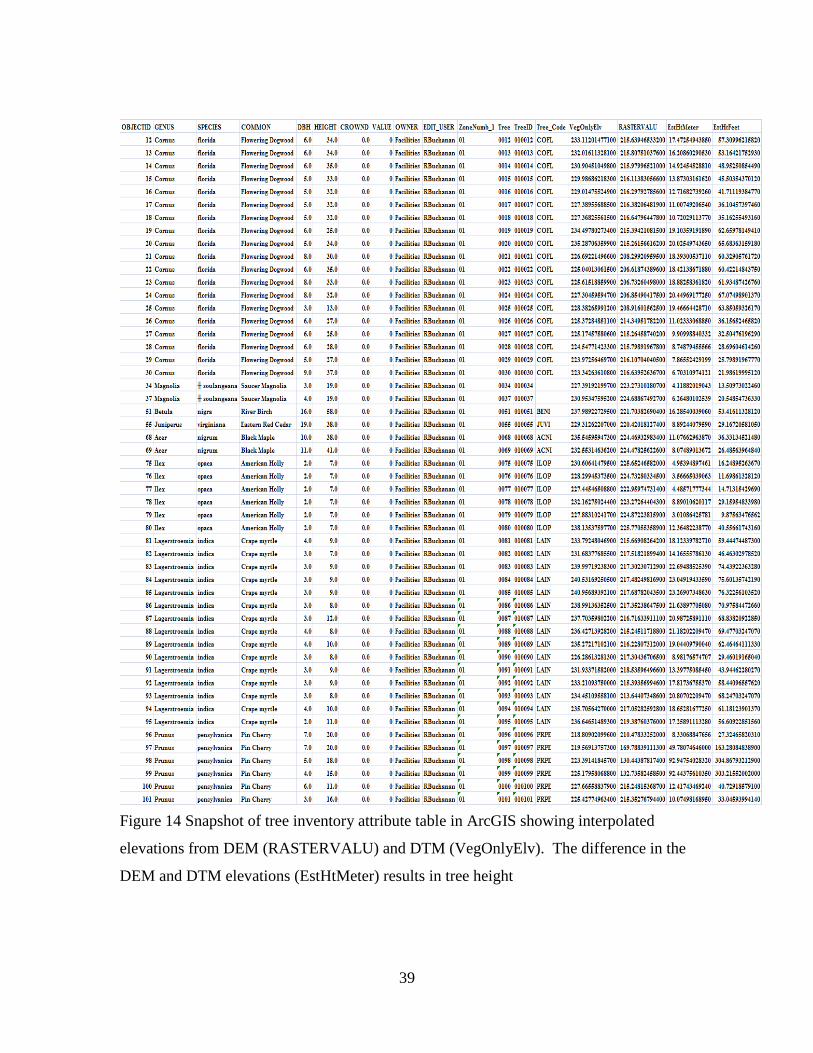
collections and unclassified points caused varying levels of inaccuracy. UAV point cloud

processing with LASTools reduced many of these inaccuracies. Tree heights were

interpolated and incorporated as an attribute in the tree inventory feature class (Figure

14). Descriptive statistics were calculated on the filtered results for statistical analysis.

Statistical Analysis

Statistical comparisons were made between measured and estimated tree heights.

Descriptive statistics for mean, N, and standard deviation calculated in ArcGIS 10.1,

were used in a t-test calculator (GraphPad (http://www.graphpad.com/quickcalcs/ttest1/)

for p-value determination. Trees (27% of total inventory) with measured and estimated

tree heights were used for comparison of means.

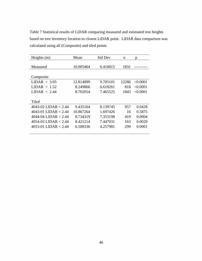
LiDAR derived CHM’s results found that tree heights were not equal to measured tree

heights (p = 0.0001) which was unexpected. LiDAR data was parsed into tiles to

determine if this was spatially consistent across the study boundary. A neighborhood

search for LiDAR values at varying distances was used to determine if position accuracy

could have caused the poor height estimates with the LIDAR data. Statistical analysis

(Table 7) for each tile shows there is an exception and spatial areas exist where tree

heights are equal (p > 0.01). These results indicate that spatial inaccuracies between the

CHM and tree location(s) provided inaccurate height results for certain spatial extents. It

is concluded if spatial alignment issues can be resolved accurate tree height values could

be interpolated.

The DEM and DSM provided from DroneMapper did not have a consistent scale

factor to convert pixel value into a usable elevation value, which made it unusable for

http://www.graphpad.com/quickcalcs/ttest1/

23

estimating tree heights. A gridded method was used to construct a model to compare

grass or open areas to building tops. If the scale factor for each classification is equal the

derived scale then it could be used to convert pixel values. GraphPad was used to

compare two means using a t-test. The results (Table 8) show that both scale factors are

equal (p = 0.056). Further testing is needed to determine if the scale factor is valid for

both the DEM and DSM models and if a variable scale factor would be necessary.

The results (Table 9) of LASTool processing of the Agisoft point cloud concluded at

the level of significance (α = 0.01) that the measured and estimated tree heights were

equal (p = 0.7641). These statistical results show that using the point cloud from high

resolution imagery can be accurate for tree height determination. Further statistical

testing was performed stratifying the measured height sample to look at individual tree

species. Individual species (70.2% of all species with measured heights) with n > 1 were

tested to compare measured and estimated tree height means. This testing (α = 0.01)

show that 82% of individual species had equal means (Table 10). The 18% with unequal

means include Cornus florida, Ilex opaca, Lagertroemia indica, Magnolia virginiana,

Quercus alba, Pinus teada, and Thuja occidentalis. Three species, Pinus teada, Quercus

alba and Thuja occidentalis showed measured mean values higher (22%, 20% and 40%

respectively) than estimated means. In contrast, Cornus florida, Ilex opaca,

Lagertroemia indica and Magnolia virginiana, showed higher estimated means (42%,

31%, 21%, and 54%, respectively).

Multiple statistical and physical characteristics were examined to determine factors

that could have explained the seven species with unequal means. Plausible explanations

24

indicate that no single factor contributes to the error in height estimation. A combination

of factors likely caused the error. Stratifying the data by species, an evaluation was

conducted that revealed three characteristics: sparse point cloud, tree point proximity (< 5

m) to buildings and miss-classified/unclassified points as probable causes of error. When

examining these factors, adjoining point values influenced estimated tree height results.

Proximity to buildings caused estimated tree heights to increase while areas of little to no

points (sparse point cloud) caused measured heights to be greater than estimated heights.

Miss-classified and unclassified points could cause either height value to increase over

the other and is dependent upon closest point to actual tree location. Additional analysis

was conducted spatially adjusting (increased neighborhood size to 1meter from 25

centimeters) DEM parameters in an attempt to increase accuracy among estimated

heights. Statistical analysis for all species revealed at the level of significance (α = 0.01)

estimated and measured tree heights were still equal (p = 0.9628). Comparing the seven

species with unequal means, statistically they remained unequal (p = 0.0001). It was

observed that 71% of the individual species showed estimated height means were higher

than measured means. For these species distance to buildings was the contributing factor

as elevation points representing the building influenced (increasing) estimated tree

height. The other 29% of species show mean measured heights greater than mean

estimated heights. This was due to sparse point cloud and miss-classified points

influencing (decreasing) estimated tree heights.

25

CHAPTER 4

CONCLUSION

Research objectives were to evaluate UAV implementation potential within the urban

forest, build a tree inventory and develop a tree height model from an imagery derived

point cloud. The UAV proved to be an effective tool to acquire high resolution imagery.

Agisoft rendered orthomosic photos that had high spatial and tonal accuracies. Findings

include that ground control points are required to provide spatial accuracy needed for

imagery and terrain model correlation to tree position(s). Tree inventory acquisition

using the high-resolution UAV imagery and resulting point cloud was simple with

increased efficiency resulting in time savings over traditional methods. Tree height

model processing had varied results depending on software used. Future opportunities

exist to uncover deficiencies related to height modeling within different software

applications. Agisoft mosaic generation provided the best solution for image processing

and point cloud extraction. LASTools proved to be effective in producing accurate tree

heights (p = 0.7641) from UAV point clouds. Due to inequality with several individual

tree species it is suggested that parameters for point cloud creation and classification

needs user customization to account for factors contributing to their difference of means.

This study has shown how the UAV can improve tree inventory workflows while

generating a higher degree of visibility to assist in effective management decisions.

26

Figure 1 General classification categories of UAV’s

Fixed Wing Swinglet Cam http://www.sensefly.com/products/swinglet-cam

Multicopter http://diydrones.com/profiles/blogs/a-newbies-guide-to-uavs

http://www.sensefly.com/products/swinglet-cam

http://diydrones.com/profiles/blogs/a-newbies-guide-to-uavs

27

Figure 2 LiDAR returns when laser pulses hit the ground and trees (FRA, 2014)

28

Figure 3 Study boundary used for UAV implementation to collect high resolution

imagery for developing a tree inventory and tree height model. Green dots represent

geodetic control locations

29

Figure 4 Ground control station for Sensefly Swinglet UAV. The control station provides

continuous flight monitoring and UAV control

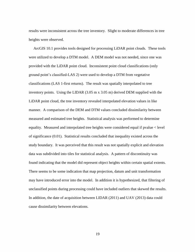
30

Figure 5 Screen capture of Emotion2 software (Sensefly, Inc.) during aerial photo

mission. The screen contains flight controls, current mission parameters, communication

limits, and flight path(s)

31

Figure 6 Tonal imbalances and spatial alignment inaccuracies occurring between flights

following image processing

32

Figure 7 Completed georeference mosaic of Clemson University. This seamless

orthomosaic was used for tree inventory acquisition

33

Figure 8 Tree inventory results using high resolution mosaic of Clemson campus

34

OBJECTID GENUS SPECIES COMMON DBH HEIGHT CROWND LOC_VALUE CONDITION INSPE_ZONE VALUE OWNER EDIT_USER ZoneNumb_1 Tree TreeID Tree_Code

12 Cornus florida Flowering Dogwood 6.0 34.0 0.0 0 0 0 0 Facilities RBuchanan 01 0012 010012 COFL



















34 Magnolia ╫ soulangeana Saucer Magnolia 3.0 19.0 0.0 0 0 0 0 Facilities RBuchanan 01 0034 010034

37 Magnolia ╫ soulangeana Saucer Magnolia 4.0 19.0 0.0 0 0 0 0 Facilities RBuchanan 01 0037 010037

51 Betula nigra River Birch 16.0 58.0 0.0 0 0 0 0 Facilities RBuchanan 01 0051 010051 BENI

55 Juniperus virginiana Eastern Red Cedar 19.0 38.0 0.0 0 0 0 0 Facilities RBuchanan 01 0055 010055 JUVI

68 Acer nigrum Black Maple 10.0 38.0 0.0 0 0 0 0 Facilities RBuchanan 01 0068 010068 ACNI

69 Acer nigrum Black Maple 11.0 41.0 0.0 0 0 0 0 Facilities RBuchanan 01 0069 010069 ACNI

75 Ilex opaca American Holly 2.0 7.0 0.0 0 0 0 0 Facilities RBuchanan 01 0075 010075 ILOP






81 Lagerstroemia indica Crape myrtle 4.0 9.0 0.0 0 0 0 0 Facilities RBuchanan 01 0081 010081 LAIN















96 Prunus pensylvanica Pin Cherry 7.0 20.0 0.0 0 0 0 0 Facilities RBuchanan 01 0096 010096 PRPE






Figure 9 Screen capture of tree inventory attribute table in ArcGIS after field data was

collected and keycoded as values into the table

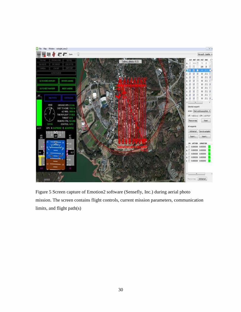
35

Figure 10 Spatial comparison of Dronemapper point cloud (blue) with tree inventory

(red)

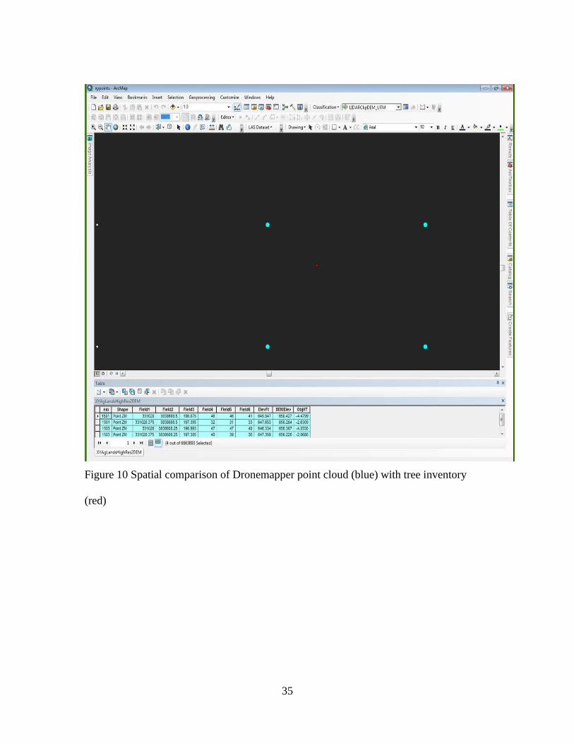
36

Figure 11 TiFFS output using LiDAR point cloud showing trees (blue) and canopy

(green) Trees (red) identified during UAV inventory process are shown for spatial

comparison

37

Figure 12 UAV point cloud (DroneMapper) results (blue) using TiFFS showing spatial

inaccuracies when compared to tree inventory (red) results

38

Figure 13 Fusion canopy height model (CHM) results with UAV tree inventory

(measured trees -red, unmeasured trees-green) used for spatial comparison

39

Figure 14 Snapshot of tree inventory attribute table in ArcGIS showing interpolated

elevations from DEM (RASTERVALU) and DTM (VegOnlyElv). The difference in the

DEM and DTM elevations (EstHtMeter) results in tree height

40

Table 1 Unmanned aerial vehicle (UAV) products related to Urban Forestry uses

UAV products Urban forestry uses

Color aerial photography

- Land cover/use mapping

- Tree inventory

- Historical documentation

- Vegetation analysis (crown density)

- Temporal comparison

- Planning

- Maintenance

- Planting

- Wildlife corridors

- Landscape fragmentation

Near Infrared (NIR) photography - Vegetation analysis

- Tree monitoring

- Vegetation health monitoring (e.g. insect/disease

detection)

LiDAR - Tree heights

- Topographic analysis

- Watershed analysis

- Infrastructure analysis

- Soil moisture,

- Forest structure

- Riparian analysis

DEM - 3D modeling

- Contours

- Road/trail design

- Slope/aspect

- Elevation

Thermal imaging - Vegetative analysis,

- Insect/disease monitoring

- Drought sensitivity

Note: Digital elevation model (DEM) is a product of color images and is used to support

other analysis. Technology for LiDAR sensors are creating smaller packages which in

time can be incorporated into a UAV platform.

41

Table 2 Benefits for having a tree inventory (adapted from NCFS, 2014)

Benefits Examples

Liability Mitigation Maintenance

Complaints

Site visits

Tree inspection

Budget Considerations Economic value

Value-engineered budget allocations

Budget awareness for maintenance and planting

Planning Estimated potential

Future strategies

Diversity allocation

42

Table 3 American Society of Photogrammetry and Remote Sensing (ASPRS) Standard

LiDAR Point Classes (ESRI, 2014)

Classification Code Classification type

0 Never classified

1 Unassigned

2 Ground

3 Low Vegetation

4 Medium Vegetation

5 High Vegetation

6 Building

7 Noise

8 Model Key

9 Water

10 Reserved for ASPRS Definition

11 Reserved for ASPRS Definition

12 Overlap

13–31 Reserved for ASPRS Definition

43

Table 4 Arial coverage by UAV flights in summer of 2013

Flight Number of photos Date

F01 401 7/17/2013

F02 337 7/17/2013

F03 110 7/17/2013

F001 153 7/17/2013

F002 73 7/17/2013

F01 204 7/19/2013

F02 161 7/19/2013

F01 240 10/1/2013

F02 95 10/1/2013

F01 59 10/2/2013

F02 189 10/2/2013

F01 245 10/3/2013

F02 256 10/3/2013

F01 208 10/4/2013

F02 259 10/4/2013

F01 100 10/18/2013

F02 82 10/18/2013

F01 107 10/29/2013

F02 167 10/29/2013

Total 3446 -------------

44

Table 5 Comparative analyses between UAV and field tree inventory techniques for

summer 2013 flight mission

Parameter UAV image Field identification

Total trees identified: 6700 5360 1340

Identification time per tree 22.8 sec/tree 2.1 min/tree

Total tree time cost 5.3 days 29.3 days

45

Table 6 Flow design of processing UAV point cloud using LASTools to classify points

into ground and high vegetation to produce DTM and DEM models

Step Input File Tool Output File

1 pointcloud.txt TXT2LAS pointcloud.las

2 pointcloud.las LAS2LAS pointcloud_prj.las

3 pointcloud_prj.las LASTILE Muliple _temp.las files

4 Multiple las Files LASGROUNDPRO Multiple _tile_g.las files

5 Multiple _tile_g.las files LASHEIGHTPRO Multiple _temp_g_h.las Files

6 Multiple _temp_g_h.las Files LASCLASSIFYPRO Multiple _temp_g_h_c.las Files

7 Multiple _temp_g_h_c.las Files LAS2DEMPRO Multiple _temp_DEM Files

8 Multiple _temp_g_h_c.las Files LAS2DEMPRO Multiple _temp_DTM Files

9 Multiple _temp_DEM Files Mosaic pointcloud_DEM

10 Multiple _temp_DTM Files Mosaic pointcloud_DTM

11 pointcloud_DEM Extract Values to Points TreePoints_DEM

treeinventory feature class

12 pointcloud_DTM Extract Values to Points TreePoints_DEM_DTM

TreePoints_DEM

46

Table 7 Statistical results of LiDAR comparing measured and estimated tree heights

based on tree inventory location to closest LiDAR point. LiDAR data comparison was

calculated using all (Composite) and tiled points

Heights (m) Mean Std Dev n p

Measured 10.005464 6.416815 1831 ----------

Composite

LIDAR < 3.05 12.814899 9.705101 12286 <0.0001

LIDAR < 1.52 8.249866 6.618261 818 <0.0001

LIDAR < 2.44 8.702054 7.465525 1843 <0.0001

Tiled

4043-02 LIDAR < 2.44 9.435164 8.139745 957 0.0428

4043-01 LIDAR < 2.44 10.867264 1.697426 16 0.5875

4044-04 LIDAR < 2.44 8.734319 7.353198 419 0.0004

4054-03 LIDAR < 2.44 8.421214 7.447031 163 0.0029

4053-01 LIDAR < 2.44 6.508336 4.257981 299 0.0001

47

Table 8 Statistical comparison of grass and building values to develop a scale factor for

pixel conversion to actual elevation heights

Mean Std Dev n p

Grass 3.59688 0.733275 407 0.056

Building 3.810796 2.123046 380 --------

48

Table 9 Statistical results of comparing measured and estimated tree heights using

Agisoft/LASTool point cloud analysis interpolated to tree inventory points

Heights(m) Mean StdDev n p

Measured 9.997911 6.395687 1814 ---------

Estimated 10.066329 7.303170 1814 0.7641

49

Table 10 Comparison of means for individual tree species that have measured and

estimated heights

Species

% of

Total Measured Heights (m) Estimated Heights (m)

Mean StdDev n Mean StdDev n p

Acer ginnala 1.28 4.37605719 0.75198153 14 4.3899488 1.22707024 14 0.972

Acer nigrum 6.59 13.8091335 4.15245774 72 12.863055 4.60020711 72 0.197

Acer palmatum 0.73 3.8862 1.04201946 8 6.4467705 2.93613941 8 0.036

Acer rubrum 9.33 8.91390587 4.32538053 102 7.7796987 4.52671678 102 0.069

Acer

saccharinum 0.18 11.8872 1.8288 2 16.115983 4.98739333 2 0.378

Aquifolaceae

ilex 12.35 6.95621327 2.62169118 135 7.9871215 3.85926726 135 0.011

Betula nigra 1.10 11.7094001 3.90425361 12 13.637374 3.56710823 12 0.22

Carya

illnoinensis 1.37 18.57248 8.54996461 15 16.562615 8.05530561 15 0.513

Cedrus

deodara 1.65 13.5974666 7.54727228 18 12.119252 7.07711158 18 0.573

Cercis

canadensis 0.37 8.4582 1.72925323 4 5.4733908 1.75409657 4 0.052

Cornus florida 4.30 7.24386674 2.58647641 47 12.69317 6.6115884 47 0.0001

Cupressus x

leylandii 1.92 9.28914271 3.01534068 21 10.650126 3.00641278 21 0.151

Fagus

grandifolia 0.64 5.74765719 4.21219488 7 7.1562748 4.22674969 7 0.544

Ginkgo bibola 1.28 9.2964 4.15332428 14 8.7577672 4.15367998 14 0.734

Juniperus

virginiana 0.27 16.1544 4.66254358 3 14.178036 4.07077716 3 0.61

Ilex opaca 10.43 7.01842112 2.01473227 114 10.293291 5.46253477 114 0.0001

Lagerstroemia

indica 31.11 5.70872478 1.72064812 340 7.3093856 4.40564077 340 0.0001

Liquidambar

styraciflua 0.18 21.336 2.7432 2 15.552559 3.36119236 2 0.2

Magnolia

grandiflora 4.12 10.24128 4.03872466 45 13.169164 9.51982358 45 0.061

Magnolia x

soulangeana 0.46 7.0104 1.27870763 5 5.841955 1.09522382 5 0.159

Magnolia

virginiana 2.29 3.47472 0.58775041 25 7.6909931 4.6599284 25 0.0001

Quercus alba 12.90 18.6187403 8.62923736 141 14.882221 10.463966 141 0.001

Querecus

coccinea 1.83 12.55776 3.45191883 20 13.020363 5.22263827 20 0.743

Quercus

falcata 0.27 15.4432001 4.23319773 3 14.944955 2.61896261 3 0.871

Quercus

glauca 0.27 6.4008 1.08479112 3 8.4583036 2.62126119 3 0.277

Quercus

macrocarpa 0.82 10.0584 3.01394317 9 10.048625 3.80715012 9 0.995

Quercus 0.82 13.3434667 1.01373981 9 13.370267 2.23069831 9 0.974

50

palustris

Quercus nigra 1.10 17.653001 3.3399792 12 14.687491 6.12000513 12 0.1548

Quercus

virginiana 0.73 13.4112 2.23981335 8 14.455445 3.80807519 8 0.5147

Parrotia

persica 0.55 4.0132001 1.22448036 6 4.7621269 1.87422465 6 0.432

Pinus taeda 11.71 5.5387875 1.34494036 128 4.2771447 1.60987801 128 0.0001

Pinus

virginiana 0.27 14.2240001 0.57473637 3 15.729783 0.83668149 3 0.062

Prunus

pensylvanica 3.02 6.14218177 2.39544332 33 14.243165 21.635794 33 0.036

Prunus x

yedoensis 2.20 5.6134001 1.34572065 24 7.0661031 3.83576231 24 0.087

Pyrus

calleryana 0.37 12.192 1.27506984 4 17.183432 6.05538967 4 0.158

Taxodium

distichum 4.12 8.2499201 4.04587466 45 8.4800145 5.11828237 45 0.814

Thuja

occidentalis 1.19 5.55673839 0.2714241 13 3.2774434 0.87714734 13 0.0001

Thuja spp. 0.18 5.4864 0.6096 2 3.0650798 0.56440791 2 0.054

Tilia

heterophylla 0.27 13.8175999 2.72999789 3 12.536152 4.51010945 3 0.695

Ulmus

parvifolia 5.03 8.23514187 1.3809473 55 7.2475688 1.50065567 55 0.0005

Unknown 1.56 8.44475283 3.28073949 17 6.9956836 3.35958546 17 0.212

Total 100.00

1093

Note: Species with p shown in red have measured heights ≠ estimated heights.

51

APPENDIX

Glossary

American Standard Code (ASCII):

code that is used for information exchange and is based on the English alphabet

using 128 specified characters, 0-9 numbers, letters a-z, and letters A-Z

Agisoft:

a commercial based 3D reconstruction software that uses digital photos.

The professional edition allows authoring of geographic information system (GIS)

data to produce seamless imagery and 3D point clouds

ArcGIS:

a commercial based geographic information system (GIS) developed by

Environmental Systems Research Institute

Autonomous:

operation of a UAV by onboard computer or ground based pilot by remote control

Canopy:

uppermost layer of the forest formed by tree crowns

Canopy Height Model (CHM):

raster based model representing the canopy elevation of the forest and or trees

Diameter at Breast Height (DBH):

measurement location to obtain tree diameter usually at 4.5’ off the ground

Digital Elevation Model (DEM):

raster based model representing ground or surface elevations

Digital Terrain Model (DTM):

raster based model representing vegetation height elevations

DroneMapper:

commercial based software for geo-spatial mapping of aerial imagery to produce

orthomosaic, digital elevation and digital surface models

52

Federal Aviation Administration (FAA):

government agency charged with the primary responsibility for safety,

advancement and regulation related to civil aviation

Fusion:

free software developed by the United States Forest Service to view and

analyze LiDAR data

Geodetic Control Point (GCP):

global positioning system (GPS) derived point that

can be used to accurately position non-spatially referenced geographic data by

serving as reference object that can be tied to its complimentary location in

geographic data

Geographic Information System (GIS):

a computer based software that captures, manages, analyzes, edits and displays

geographic data

Geotagging:

process of adding geographic metadata to photographs or imagery

Global Positioning System (GPS):

satellite based navigation system that provides locational information

Ground Control Station:

facilities and computer hardware that maintains human control over unmanned

aerial vehicles during flight

Heads-Up-Digitizing:

GIS process for creating feature objects from data (i.e. imagery) displayed on a

computer screen

Hyperspectral:

imaging technique that collects data by scanning objects across the

electromagnetic spectrum using three techniques: scanning spatial images,

sequential capture of full spectral data, or capture spatial and spectral data at the

same time

53

Imagery:

images representing spatial objects on the earth’s surface

LASTools:

toolset developed by Martin Isenburg for LiDAR las formatted data. Can be used

through DOS command window and as a toolkit or pipeline in ArcGIS

Light Detection and Ranging (LiDAR):

remote sensing technique that uses a laser to measure distance by analyzing

reflected light of a laser illuminated object on the earth

Log ASCII Standard (LAS):

standard file format for exchanging LiDAR data

Mosaic:

process of creating a single image from a collection of images

Multi-Spectral:

process of capturing image data at specific frequencies of the electromagnetic

spectrum

Multi-Temporal:

data that contains information which spans across different time ranges i.e.

multiply years

National Airspace System (NAS):

constitutes the facilities, systems, equipment, procedures, and airports for a flying

environment that is safe and efficient

Near Infrared (NIR):

image data collected in the near infrared region of the electromagnetic spectrum

this is closest to the radiation detected by the human eye

Orthomosaic:

combination of orthorectification and mosaicing to create a rectified image with

limited distortion to form a single image from a collection of images

54

Orthorectification :

process of correcting imagery distortion by using based data such as elevation

along with camera metadata to match map projection

Photogrammetry:

the scientific process(s) of developing measurements from photographs

Point Cloud:

consists of data points referenced to a coordinate system so that each point

contains a value for the x, y, and z

Random Access Memory (RAM):

a type of computer data storage for accessing and writing data at the same speed

regardless of the order it is accessed

Spatialtemporal:

term used to describe spatial data over a period of time

Soil Type:

defines a soil based upon the soil texture or the size of minerals contained within

a soil sample

Soil Volume:

the amount of soil available for a plant to grow into

Structured Query Language (SQL):

programming language used to managing data within a relational database

Toolbox for LiDAR Data Filtering and Forest Studies (TiFFS):

commercial based computer software for automatic viewing and analysis of

LiDAR point clouds

Urban Forest:

a collection of trees or forest stands within a city, town or suburb

Unmanned Aerial Vehicle (UAV):

term used to describe a remotely operated airborne vehicle that is flown in

absence of a human pilot

55

Unmanned Aerial System (UAS):

ground control equipment, communication system and other support equipment

including the unmanned aerial vehicle to maintain flight mission objectives

X,Y:

coordinate pair point representing values of a map projection that spatially locates

an object on the earth’s surface

Z-Value:

spatial value of a map projection that represents elevation of a located object

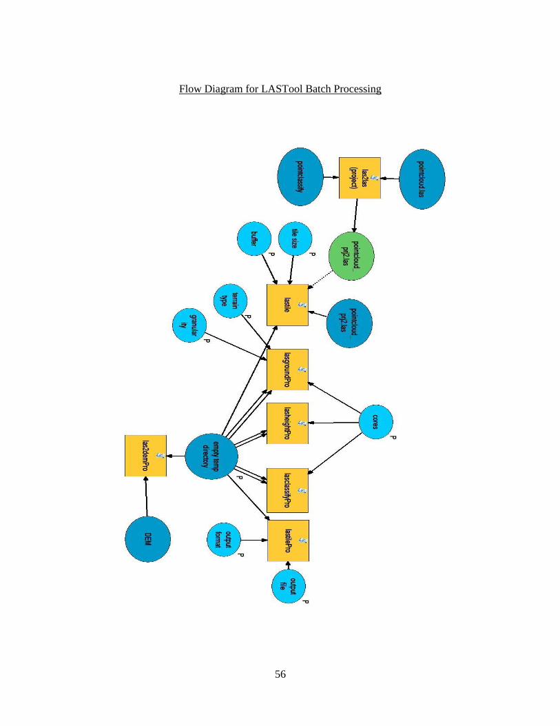
56

Flow Diagram for LASTool Batch Processing

57

REFERENCES

American Society for Photogrammetry and Remote Sensing (ASPRS), 2012. LASer

(LAS) File Format Exchange Activities. Available online at

http://www.asprs.org/Committee-General/LASer-LAS-File-Format-Exchange-

Activities.html

Anderson, Karen, Gaston, Kevin, 2013. Lightweight unmanned aerial vehicles will

revolutionize spatial ecology. Front Ecol Environ 11; 11(3): 138-146, doi:

10.1890/120150, March 18 2013.

Arjomandi, M. 2007. Classification of Unmanned Aerial Vehicles. The University of

Adelaide, Australia.

Black, Justin, 2014. Measuring Tree Volume with a Biltmore Stick. Utah State

University. Available online at http://forestry.usu.edu/htm/rural-forests/forest-

management/forest-timber-management/measuring-tree-volume-with-a-biltmore-

stick/

Blom, John David, 2010. Unmanned Aerial Systems: A Historical Perspective.

Occasional Paper 37, Combat Studies Institute Press. US Army Combined Arms

Center, Fort Leavenworth Kansas.

Chen, Qi, 2007. Airborne LiDAR Data Processing and Information Extraction. Journal

of Photogrammetric Engineering and Remote Sensing, February, 2007.

Clemson, 2013. Clemson University Website History Page;

http://www.clemson.edu/about/history/ About the Clemson University Land Use

Property Page; http://www.clemson.edu/administration/public-

affairs/landuse/about.html Graduate School Information page;

http://www.grad.clemson.edu/GeneralInformation.php

DIY, 2013. DIY Drones website by Chris Anderson. http://diydrones.com/

Elias, B. 2012. Pilotless Drones: Background and Considerations for Congress

Regarding Unmanned Aircraft Operations in the National Airspace System. CRS

Report for Congress, Congressional Research Service 7-5700, September 10,

2012.

Ellison, M. J. (2005). Quantified tree risk assessment used in the management of amenity

trees. Journal of Arboriculture, 31(2), 57-654. Available online at

http://www.qtra.co.uk/docs/QTRA.pdf

http://www.asprs.org/Committee-General/LASer-LAS-File-Format-Exchange-Activities.html

http://www.asprs.org/Committee-General/LASer-LAS-File-Format-Exchange-Activities.html

http://forestry.usu.edu/htm/rural-forests/forest-management/forest-timber-management/measuring-tree-volume-with-a-biltmore-stick/



http://www.clemson.edu/about/history/

http://www.clemson.edu/administration/public-affairs/landuse/about.html

http://www.clemson.edu/administration/public-affairs/landuse/about.html

http://www.grad.clemson.edu/GeneralInformation.php

http://diydrones.com/

http://www.qtra.co.uk/docs/QTRA.pdf

58

Environmental Systems Resource Institute (ESRI), 2014. Online ArcGIS Resource

Center. Help Desk ArcGIS version 10.2. Available online at

http://resources.arcgis.com/en/help/main/10.2/index.html#//00qn0000001p000000

Eugster, H., & Nebiker, S. (2008). UAV-Based Augmented Monitoring-Real-Time

Georeferencing and Integration of Video Imagery with Virtual Globes. IAPRSSIS,

37(B1), 1229-1235.

Forest Resource Assessment Nepal, 2014. LiDAR Assisted Multisource Programme in

TAL. Available online at http://www.franepal.org/?page_id=135

GAO, 2012. Measuring Progress and Addressing Potential Privacy Concerns Would

Facilitate Integration into the National Airspace System US Accountability

Office report to Congress. [Reissued on September 18, 2012] GAO-12-981, Sep

14, 2012 Available online at http://www.gao.gov/assets/650/648348.pdf

Globalidar, 2014. TIFFS, The Lidar Information Engine. Available online at

http://www.globalidar.com/Pages/default.aspx

Harwin, S., Lucieer, A. 2012. Assessing the accuracy of georeferenced point clouds

produced via multi-view stereopsis from unmanned aerial vehicle (UAV)

imagery. Remote Sensing, 4(6), 1573-1599.

Hunt, E. R., Hively, W. D., Fujikawa, S. J., Linden, D. S., Daughtry, C. S., & McCarty,

G. W. (2010). Acquisition of NIR-green-blue digital photographs from unmanned

aircraft for crop monitoring. Remote Sensing, 2(1), 290-305.

International Society of Arboriculture 2013. Using the ISA Basic Tree Risk Assessment

Form. Available online at http://www.isa-

arbor.com/education/resources/isabasictreeriskassessmentform_instructions.pdf

Jomaa Ihab, Auda Yves, Saleh Bernadette Abi, Hamze, & Safi, Samir, 2008. Landscape

spatial dynamics over 38 years under natural and anthropogenic pressures in

Mount Lebanon. Landscape and Urban Planning, 87: 67-75.

Johnston, L. F., Herwitz, S., Dunagan, S., Lobitz, B., Sullivan, D., Slye, R., 2003.

Collection of Ultra High Spatial and Spectral Resolution Image Data over

California Vineyards with a Small UAV. Proceedings, International Symposium

on Remote Sensing of Environment, 2003. Available online at http://www.uav-

applications.org/gallery/img/5.pdf

http://resources.arcgis.com/en/help/main/10.2/index.html#//00qn0000001p000000

http://www.franepal.org/?page_id=135

http://www.gao.gov/assets/650/648348.pdf

http://www.globalidar.com/Pages/default.aspx

http://www.isa-arbor.com/education/resources/isabasictreeriskassessmentform_instructions.pdf

http://www.isa-arbor.com/education/resources/isabasictreeriskassessmentform_instructions.pdf

http://www.uav-applications.org/gallery/img/5.pdf

http://www.uav-applications.org/gallery/img/5.pdf

59

Laliberte, A. S., Winters, C., & Rango, A. 2008. A procedure for orthorectification of

sub-decimeter resolution imagery obtained with an unmanned aerial vehicle

(UAV). In Proceedings of ASPRS Annual Conference (p. 9) April 2008.

Merino, L., Caballero, F., Martinez-de Dios, J. R., Ferruz, J., Ollero, A. 2006. A

cooperative perception system for multiple UAVs: Application to automatic

detection of forest fires. Journal of Field Robotics, Vol. 23, Iss. 3-4, March-April

2006 pp. 165-184, Available online at http://www3.interscience.wiley.com/cgi-

bin/jhome/111090262 Wiley Periodicals Inc.

Mitchell, M. 2012. President Obama Signs The FAA Modernization And Reform Act Of

2012 (H.R. 658). Aviation Online Magazine, February 15, 2012. Available

online at

http://avstop.com/news_february_2012/president_obama_signs_the_faa_moderni

zation_and_reform_act_of_2012_hr_658.htm

National Oceanic and Atmospheric Administration (NOAA), 2013. LIDAR—Light

Detection and Ranging—is a remote sensing method used to examine the surface

of the Earth. Available online at http://oceanservice.noaa.gov/facts/lidar.html

North Carolina Forest Service (NCFS) 2014. Urban and Community Tree Inventories.

Available online at

http://www.ncforestservice.gov/Urban/urban_tree_inventories.htm

Pokorny, Jill; O''Brien, Joseph; Hauer, Richard; Johnson, Gary; Albers, Jana; Bedker,

Peter; Mielke, Manfred 2003. Urban Tree Risk Management: A Community

Guide to Program Design and Implementation. USDA Forest Service

Northeastern Area State and Private Forestry 1992 Folwell Ave. St. Paul, MN

55108

Pudelko, Rafal, Stuczynski, Tomasz, Borzecka-Walker, Magdalena, 2012, The suitability

of an unmanned aerial vehicle (UAV) for the evaluation of experimental fields

and crops. Zemdirbyste=Agriculture, vol. 99, No. 4, 2012, p. 431-436.

Rango, A., and Laliberte, A. S. 2010. Impact of flight regulations on effective use of

unmanned aircraft systems for natural resources applications. Journal of Applied

Remote Sensing, 4(1), 043539-043539.

Rapidlasso, 2014. Creator of LASTools for LiDAR. http://rapidlasso.com/

Remondino, F., Barazzetti, L., Nex, F., Scaioni, M., & Sarazzi, D. 2011. UAV

photogrammetry for mapping and 3D modeling–current status and future

perspectives–. Proceedings of the International Archives of the Photogrammetry,

Remote Sensing and Spatial Information Sciences, 38, 1.

http://www3.interscience.wiley.com/cgi-bin/jhome/111090262

http://www3.interscience.wiley.com/cgi-bin/jhome/111090262

http://avstop.com/news_february_2012/president_obama_signs_the_faa_modernization_and_reform_act_of_2012_hr_658.htm

http://avstop.com/news_february_2012/president_obama_signs_the_faa_modernization_and_reform_act_of_2012_hr_658.htm

http://oceanservice.noaa.gov/facts/lidar.html

http://www.ncforestservice.gov/Urban/urban_tree_inventories.htm

http://rapidlasso.com/

60

Rowntree, R. A. 1988. Ecology of the Urban Forest: Introduction to Part III. Landscape

Urban Plann., 15:1-10.

Rudol, P., & Doherty, P., 2008. Human body detection and geolocalization for

UAV search and rescue missions using color and thermal imagery. In Aerospace

Conference, 2008 IEEE (pp. 1-8). IEEE.

United States Forest Service (USFS), 2014. LIDAR & IFSAR Tools.. U.S. Department

of Agriculture, Pacific Northwest Research Station. Available online at

http://forsys.cfr.washington.edu/JFSP06/lidar_&_ifsar_tools.htm

Wallace, L., Lucieer, A., Watson, C., & Turner, D., 2012. Development of a UAV-

LiDAR system with application to forest inventory. Remote Sens, 4(6), 1519-

1543.

Wang, Yunsheng; Weinacker, Holger; Koch, Barbara. 2008. "A Lidar Point Cloud Based

Procedure for Vertical Canopy Structure Analysis And 3D Single Tree Modeling

in Forest." Sensors 8, no. 6: 3938-3951.

Yunfei, B., Guoping, L., Chunxiang, C., Xiaowen, L., Hao, Z., Qisheng, H., ... & Chaoyi,

C., 2008. Classification of LIDAR point cloud and generation of DTM from

LIDAR height and intensity data in forested area. In ISPRS Congress

Zhou, Xiaolu, Wang, Yi-Chen, 2011. Spatial-temporal dynamics of urban green space in

response to rapid urbanization and greening policies. Landscape and Urban

Planning, 100 (2011); 268-277.

http://forsys.cfr.washington.edu/JFSP06/lidar_&_ifsar_tools.htm

use of unmanned aerial vehicles (uav) for urban tree

Documents