Use of Weighted Least Squares

In fitting models of the form yi = f(xi) + i i = 1………n,

least squares is optimal under the condition 1……….n are i.i.d. N(0, 2)

and is a reasonable fitting method when this condition is at least approximately satisfied. (Most importantly we require here that there should be no significant outliers).

In the case where we have instead 1……….n are independent N(0, i

2),

it is natural to use instead weighted least squares: choose f from within the permitted class of functions f to minimise

wi(yi-f(xi))2

Where we take wi proportional to 1/i2

(clearly only relative weights matter)

^

^

For the hill races data, it is natural to assume greater variability in the times for the longer races, with the variability perhaps proportional to the distance. We therefore try refitting the quadratic model with weights proportional to 1/distance2

> model2w = lm(time ~ -1 + dist +I(dist^2)+ climb + I(climb^2),data = hills[-18,], weights=1/dist^2)

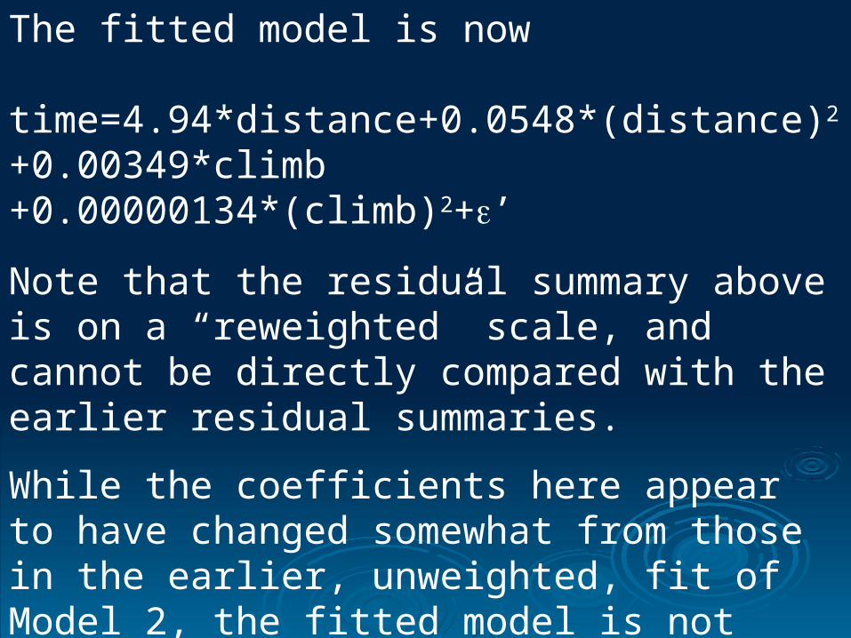
The fitted model is now

time=4.94*distance+0.0548*(distance)2+0.00349*climb +0.00000134*(climb)2+’

Note that the residual summary above is on a “reweighted” scale, and cannot be directly compared with the earlier residual summaries.

While the coefficients here appear to have changed somewhat from those in the earlier, unweighted, fit of Model 2, the fitted model is not really very different.

This is confirmed by the plot of the residuals from the weighted fit against those fromthe unweighted fit, produced by

>plot(resid(model2w)~resid(model2))

Resistant RegressionResistant Regression

As already observed, least squares fitting is very sensitive to outlying observations.

However, there are also a large number of resistant fitting techniques available. One such is least trimmed squares: choose f from within the permitted class of functions f to minimise:-

^

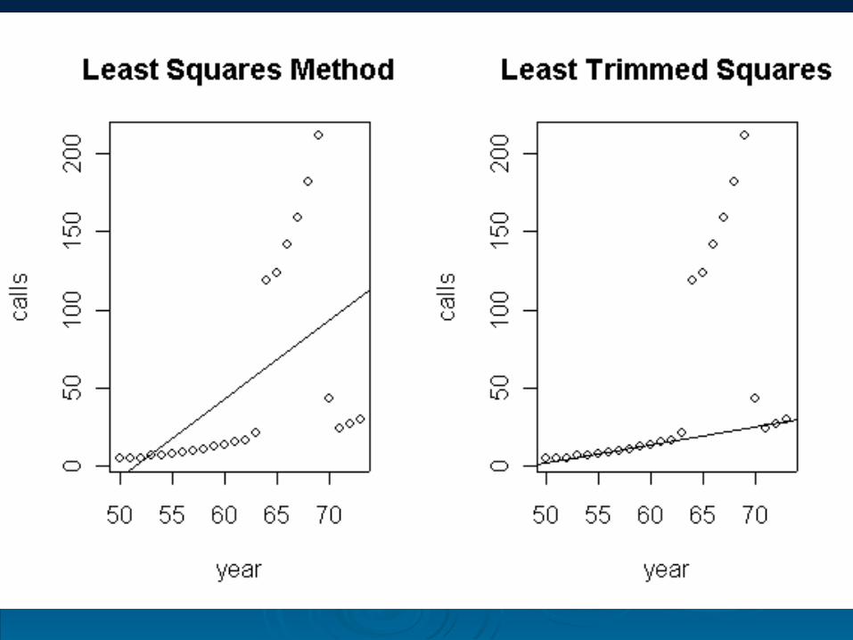
Example: phones data.

The R dataset phones in the package MASS gives the annual number of phone calls (millions) in Belgium over the period 1950-73.

Consider the modelcalls = a + b*year

The following two graphs plot the data and shows the result of fitting the model by least squares and then fitting the same model by least trimmed squares.

These graphs are achieved by the following code:

> plot(calls~year)> phonesls=lm(calls~year)> abline(phonesls)> plot(calls~year)> library(lqs)> phoneslts=lqs(calls~year)> abline(phoneslts)

The explanation for the data is that for a period of time total length of all phone calls in each year was accidentally recorded instead.

Nonparametric Nonparametric Regression Regression

Sometimes we simply wish to fit a smooth model without specifying any particular functional form for f. Again there are very many techniques here.

One such is called loess. This constructsthe fitted value f(xi) for each observation i by performing a local regression using only those observations with x values in the neighbourhood of xi (and attaching mostweight to the closest observations).

^

Example: cars data.

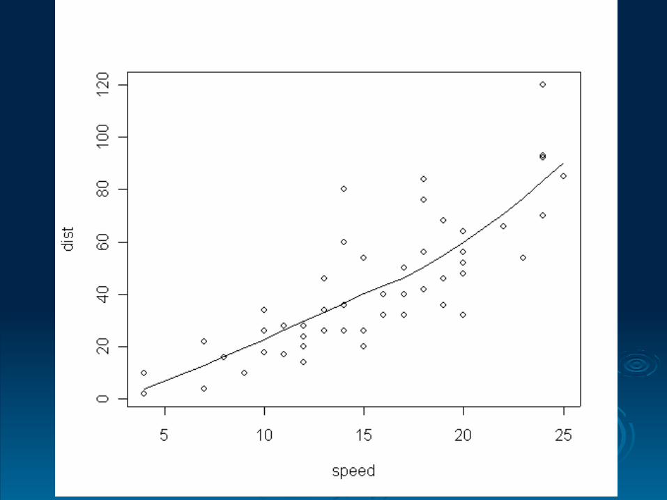
The R data frame cars (in the base package) records 50 observations of speed (mph) and stopping distance (ft). These observations were collected in the 1920s!

We treat stopping distance as the response variable and seek to model its dependence on speed.

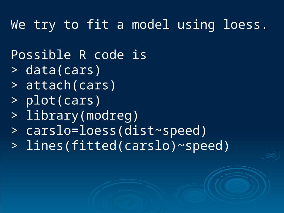
We try to fit a model using loess.

Possible R code is> data(cars)> attach(cars) > plot(cars)> library(modreg)> carslo=loess(dist~speed)> lines(fitted(carslo)~speed)

An optional argument span can be increased from its default value of 0:75 to give more smoothing:

> plot(cars)> carslo2=loess(dist~speed, span=1)> lines(fitted(carslo2)~speed)

More robust and resistant fits can be given by specifying the further optional argument family="symmetric"

Models with Qualitative Explanatory Variables (Factors)

Data: n = 22 pairs (xi , yi) where y is the response; the data arise under two different sets of conditions (type = 1 or 2) and are presented below sorted by x within type.

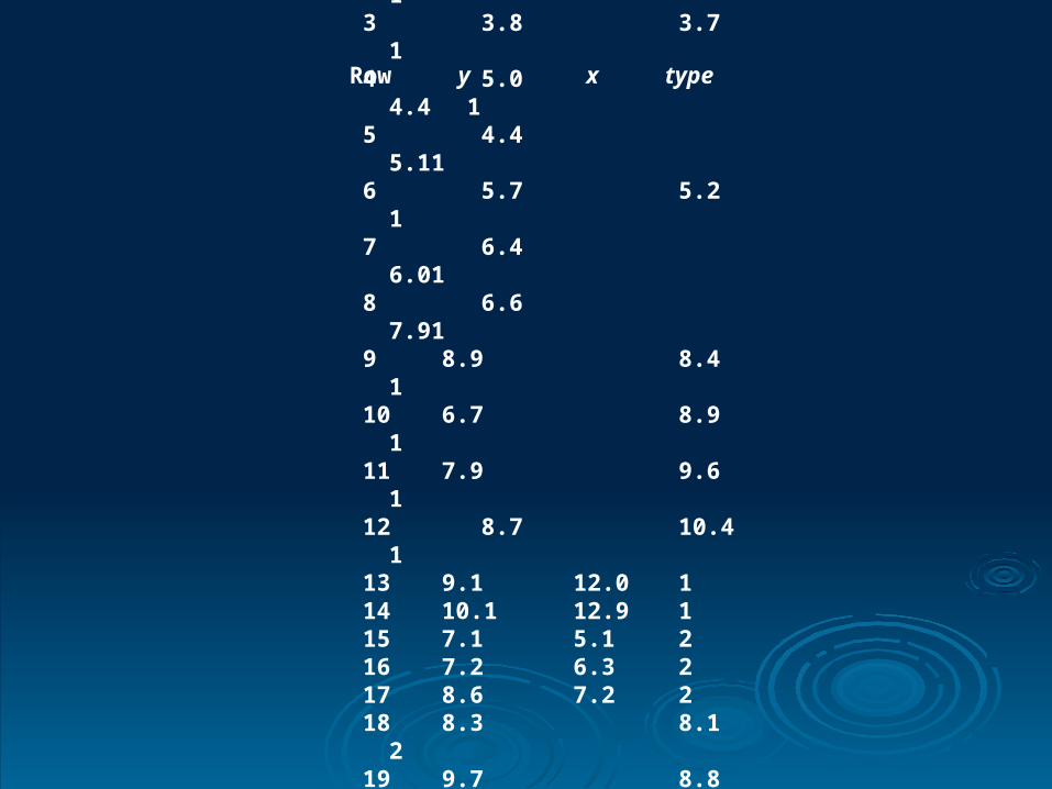
Row y x type

1 3.4 2.4 12 4.6 2.8 13 3.8 3.7 14 5.0 4.4 15 4.4 5.1 1 6 5.7 5.2 17 6.4 6.0 18 6.6 7.9 19 8.9 8.4 110 6.7 8.9 111 7.9 9.6 112 8.7 10.4 113 9.1 12.0 114 10.1 12.9 115 7.1 5.1 216 7.2 6.3 217 8.6 7.2 218 8.3 8.1 219 9.7 8.8 220 9.2 9.1 221 10.2 9.6 222 9.8 10.0 2

2 4 6 8 10 12

45

67

89

10

x

y

2 4 6 8 10 12

45

67

89

10

x1

y1

Distinguishing the two types (an appropriate R command will do this)

We model the responses first ignoring the variable type. > mod1 = lm(y~x)> abline(mod1)

2 4 6 8 10 12

45

67

89

10

x

y

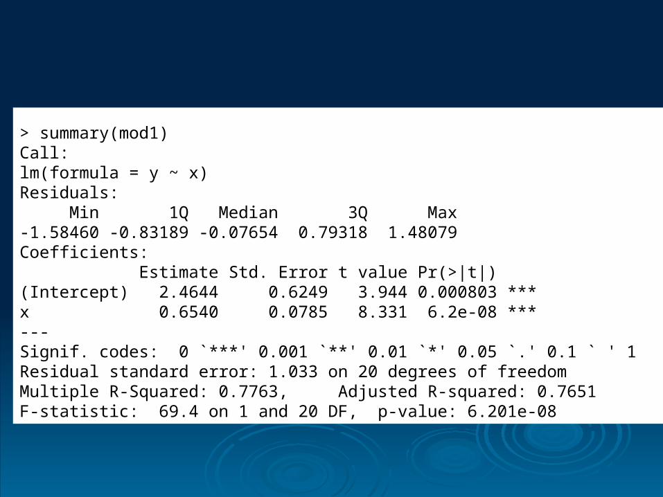
> summary(mod1)Call:lm(formula = y ~ x)Residuals: Min 1Q Median 3Q Max -1.58460 -0.83189 -0.07654 0.79318 1.48079 Coefficients: Estimate Std. Error t value Pr(>|t|) (Intercept) 2.4644 0.6249 3.944 0.000803 ***x 0.6540 0.0785 8.331 6.2e-08 ***---Signif. codes: 0 `***' 0.001 `**' 0.01 `*' 0.05 `.' 0.1 ` ' 1 Residual standard error: 1.033 on 20 degrees of freedomMultiple R-Squared: 0.7763, Adjusted R-squared: 0.7651 F-statistic: 69.4 on 1 and 20 DF, p-value: 6.201e-08

> summary.aov(mod1) Df Sum Sq Mean Sq F value Pr(>F) x 1 74.035 74.035 69.398 6.201e-08 ***Residuals 20 21.336 1.067 Signif. codes: 0 `***' 0.001 `**' 0.01 `*' 0.05 `.' 0.1 ` ' 1

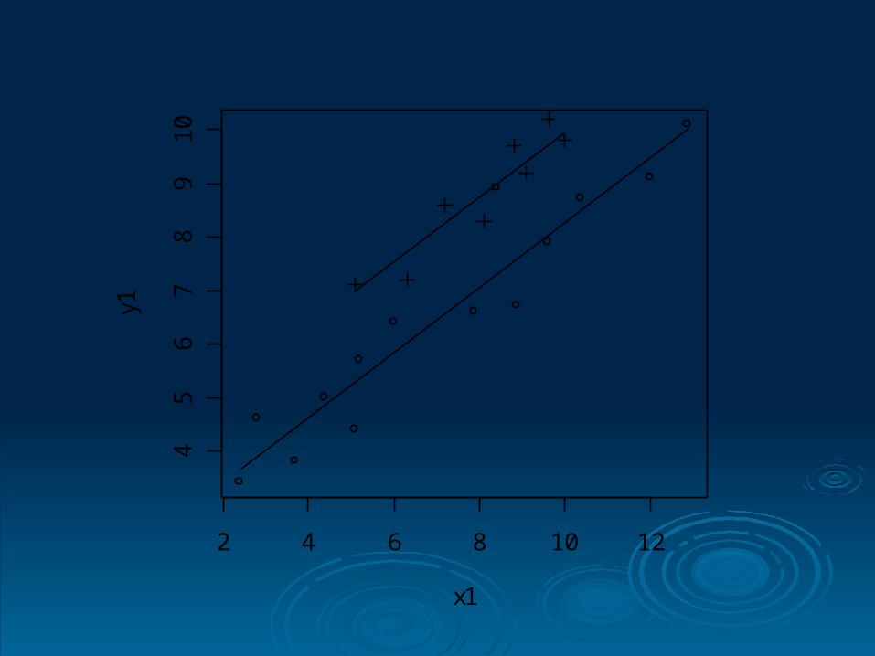
We now model the responses using a model which includes the qualitative variable type, Which was declared as a factor when the data frame was set up

> type = factor(c( rep(1,14),rep(2,8)))

>mod2 = lm(y~x+type)

> summary(mod2)Call:lm(formula = y ~ x + type)Residuals: Min 1Q Median 3Q Max -0.90463 -0.39486 -0.03586 0.34657 1.59988 Coefficients: Estimate Std. Error t value Pr(>|t|) (Intercept) 2.18426 0.37348 5.848 1.24e-05 ***x 0.60903 0.04714 12.921 7.36e-11 ***type2 1.69077 0.27486 6.151 6.52e-06 ***---Signif. codes: 0 `***' 0.001 `**' 0.01 `*' 0.05 `.' 0.1 ` ' 1 Residual standard error: 0.6127 on 19 degrees of freedomMultiple R-Squared: 0.9252, Adjusted R-squared: 0.9173 F-statistic: 117.5 on 2 and 19 DF, p-value: 2.001e-11

Interpreting the output:

The fit is ˆ 2.18426 0.60903 ( 1.69077 if type 2)y x

so e.g. observation 1 : x = 2.4, type = 1,

ˆ 2.18426 0.60903 2.4 3.646y

and for observation 20: x = 9.1, type = 2,

ˆ 2.18426 0.60903 9.1 1.69077

9.417

y

2 4 6 8 10 12

45

67

89

10

x1

y1

> summary.aov(mod2) Df Sum Sq Mean Sq F value Pr(>F) x 1 74.035 74.035 197.223 1.744e-11 ***type 1 14.204 14.204 37.838 6.522e-06 ***Residuals 19 7.132 0.375 Signif. codes: 0 `***' 0.001 `**' 0.01 `*' 0.05 `.' 0.1 ` ' 1

The fitted values for Model 2 can be obtained in R by:

>fitted.values(mod2)

1 2 3 4 5 6 7 8 3.645930 3.889543 4.437671 4.863993 5.290315 5.351218 5.838443 6.995603 9 10 11 12 13 14 15 16 7.300119 7.604634 8.030956 8.518181 9.492632 10.040760 6.981083 7.711921 17 18 19 20 21 22 8.260049 8.808177 9.234499 9.417209 9.721724 9.965337

The total variation in the responses is Syy = 95.371; variable x explains 74.035 of this total (77.6%) and the coefficient associated with it (0.6090) is highly significant (significantly different from 0) – it has a negligible P-value.

In the presence of x, type explains a further 14.204 of the total variation and its coefficient is also highly significant. Together the two variables explain 92.5% of the total variation. In the presence of x, we gain much by including type.

Finally we extend the previous model (mod2) by allowing for an interaction between the explanatory variables x and type. An interaction exists between two explanatory variables when the effect of one on a response variable is different at different values/levels of the other.

For example consider the effect of policyholder’s age and gender on a response variable claim rate. If the effect of age on claim rate is different for males and females, then there is an interaction between age and gender.

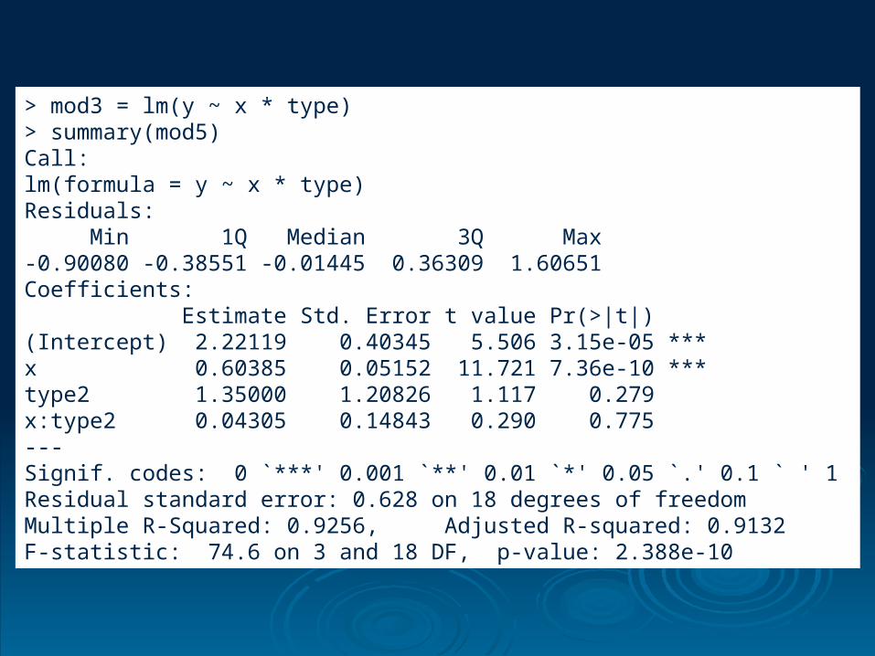
> mod3 = lm(y ~ x * type)> summary(mod5)Call:lm(formula = y ~ x * type)Residuals: Min 1Q Median 3Q Max -0.90080 -0.38551 -0.01445 0.36309 1.60651 Coefficients: Estimate Std. Error t value Pr(>|t|) (Intercept) 2.22119 0.40345 5.506 3.15e-05 ***x 0.60385 0.05152 11.721 7.36e-10 ***type2 1.35000 1.20826 1.117 0.279 x:type2 0.04305 0.14843 0.290 0.775 ---Signif. codes: 0 `***' 0.001 `**' 0.01 `*' 0.05 `.' 0.1 ` ' 1 Residual standard error: 0.628 on 18 degrees of freedomMultiple R-Squared: 0.9256, Adjusted R-squared: 0.9132 F-statistic: 74.6 on 3 and 18 DF, p-value: 2.388e-10

> summary.aov(mod5) Df Sum Sq Mean Sq F value Pr(>F) x 1 74.035 74.035 187.7155 5.810e-11 ***type 1 14.204 14.204 36.0142 1.124e-05 ***x:type 1 0.033 0.033 0.0841 0.7751 Residuals 18 7.099 0.394 ---Signif. codes: 0 `***' 0.001 `**' 0.01 `*' 0.05 `.' 0.1 ` ' 1

The interaction appears to have added nothing - the coefficient of determination is effectively unchanged compared to the previous model. We also note that the extra parameter value is small and is not significant. In this particular case, an interaction term is not helpful - including it has simply confused the issue.

In a case where an interaction term does improve the fit and the coefficient is significant, then both variables and the interaction between them should be included in the model