Use R!

Advisors:Robert Gentleman · Kurt Hornik · Giovanni Parmigiani

Use R!

Albert: Bayesian Computation with RBivand/Pebesma/Gomez-Rubio: Applied Spatial Data Analysis with RClaude: Morphometrics with RCook/Swayne: Interactive and Dynamic Graphics for Data Analysis: With R andGGobiHahne/Huber/Gentleman/Falcon: Bioconductor Case StudiesKleiber/Zeileis, Applied Econometrics with RNason: Wavelet Methods in Statistics with RParadis: Analysis of Phylogenetics and Evolution with RPeng/Dominici: Statistical Methods for Environmental Epidemiology with R: ACase Study in Air Pollution and HealthPfaff: Analysis of Integrated and Cointegrated Time Series with R, 2nd editionSarkar: Lattice: Multivariate Data Visualization with RSpector: Data Manipulation with R

Christian Kleiber · Achim Zeileis

Applied Econometrics with R

123

Christian Kleiber Achim ZeileisUniversitat Basel Wirtschaftsuniversitat WienWWZ, Department of Statistics and Econometrics Department of Statistics and MathematicsPetersgraben 51 Augasse 2–6CH-4051 Basel A-1090 WienSwitzerland AustriaChristian.Kleiber@unibas.ch Achim.Zeileis@wu-wien.ac.at

Series EditorsRobert Gentleman Kurt HornikProgram in Computational Biology Department of Statistics and MathematicsDivision of Public Health Sciences Wirtschaftsuniversitat WienFred Hutchinson Cancer Research Center Augasse 2–61100 Fairview Avenue N., M2-B876 A-1090 WienPO Box 19024, Seattle, Washington 98102-1024 AustriaUSA

Giovanni ParmigianiThe Sidney Kimmel Comprehensive Cancer Centerat Johns Hopkins University550 North BroadwayBaltimore, MD 21205-2011USA

ISBN: 978-0-387-77316-2 e-ISBN: 978-0-387-77318-6DOI: 10.1007/978-0-387-77318-6

Library of Congress Control Number: 2008934356

c© 2008 Springer Science+Business Media, LLCAll rights reserved. This work may not be translated or copied in whole or in part without the written permission of thepublisher (Springer Science+Business Media, LLC, 233 Spring Street, New York, NY 10013, USA), except for briefexcerpts in connection with reviews or scholarly analysis. Use in connection with any form of information storage andretrieval, electronic adaptation, computer software, or by similar or dissimilar methodology now known or hereafterdeveloped is forbidden.The use in this publication of trade names, trademarks, service marks, and similar terms, even if they are not identifiedas such, is not to be taken as an expression of opinion as to whether or not they are subject to proprietary rights.

Printed on acid-free paper

springer.com

Preface

R is a language and environment for data analysis and graphics. It may beconsidered an implementation of S, an award-winning language initially de-veloped at Bell Laboratories since the late 1970s. The R project was initiatedby Robert Gentleman and Ross Ihaka at the University of Auckland, NewZealand, in the early 1990s, and has been developed by an international teamsince mid-1997.

Historically, econometricians have favored other computing environments,some of which have fallen by the wayside, and also a variety of packages withcanned routines. We believe that R has great potential in econometrics, bothfor research and for teaching. There are at least three reasons for this: (1) Ris mostly platform independent and runs on Microsoft Windows, the Macfamily of operating systems, and various flavors of Unix/Linux, and also onsome more exotic platforms. (2) R is free software that can be downloadedand installed at no cost from a family of mirror sites around the globe, theComprehensive R Archive Network (CRAN); hence students can easily installit on their own machines. (3) R is open-source software, so that the full sourcecode is available and can be inspected to understand what it really does,learn from it, and modify and extend it. We also like to think that platformindependence and the open-source philosophy make R an ideal environmentfor reproducible econometric research.

This book provides an introduction to econometric computing with R; it isnot an econometrics textbook. Preferably readers have taken an introductoryeconometrics course before but not necessarily one that makes heavy use ofmatrices. However, we do assume that readers are somewhat familiar with ma-trix notation, specifically matrix representations of regression models. Thus,we hope the book might be suitable as a “second book” for a course withsufficient emphasis on applications and practical issues at the intermediateor beginning graduate level. It is hoped that it will also be useful to profes-sional economists and econometricians who wish to learn R. We cover linearregression models for cross-section and time series data as well as the com-mon nonlinear models of microeconometrics, such as logit, probit, and tobit

vi Preface

models, as well as regression models for count data. In addition, we providea chapter on programming, including simulations, optimization, and an in-troduction to Sweave()—an environment that allows integration of text andcode in a single document, thereby greatly facilitating reproducible research.(In fact, the entire book was written using Sweave() technology.)

We feel that students should be introduced to challenging data sets asearly as possible. We therefore use a number of data sets from the dataarchives of leading applied econometrics journals such as the Journal of Ap-plied Econometrics and the Journal of Business & Economic Statistics. Someof these have been used in recent textbooks, among them Baltagi (2002),Davidson and MacKinnon (2004), Greene (2003), Stock and Watson (2007),and Verbeek (2004). In addition, we provide all further data sets from Bal-tagi (2002), Franses (1998), Greene (2003), and Stock and Watson (2007),as well as selected data sets from additional sources, in an R package calledAER that accompanies this book. It is available from the CRAN servers athttp://CRAN.R-project.org/ and also contains all the code used in the fol-lowing chapters. These data sets are suitable for illustrating a wide variety oftopics, among them wage equations, growth regressions, dynamic regressionsand time series models, hedonic regressions, the demand for health care, orlabor force participation, to mention a few.

In our view, applied econometrics suffers from an underuse of graphics—one of the strengths of the R system for statistical computing and graphics.Therefore, we decided to make liberal use of graphical displays throughout,some of which are perhaps not well known.

The publisher asked for a compact treatment; however, the fact that R hasbeen mainly developed by statisticians forces us to briefly discuss a numberof statistical concepts that are not widely used among econometricians, forhistorical reasons, including factors and generalized linear models, the latterin connection with microeconometrics. We also provide a chapter on R basics(notably data structures, graphics, and basic aspects of programming) to keepthe book self-contained.

The production of the book

The entire book was typeset by the authors using LATEX and R’s Sweave()tools. Specifically, the final manuscript was compiled using R version 2.7.0,AER version 0.9-0, and the most current version (as of 2008-05-28) of all otherCRAN packages that AER depends on (or suggests). The first author startedunder Microsoft Windows XP Pro, but thanks to a case of theft he switchedto Mac OS X along the way. The second author used Debian GNU/Linuxthroughout. Thus, we can confidently assert that the book is fully repro-ducible, for the version given above, on the most important (single-user) plat-forms.

Preface vii

Settings and appearance

R is mainly run at its default settings; however, we found it convenient toemploy a few minor modifications invoked by

R> options(prompt="R> ", digits=4, show.signif.stars=FALSE)

This replaces the standard R prompt > by the more evocative R>. For compact-ness, digits = 4 reduces the number of digits shown when printing numbersfrom the default of 7. Note that this does not reduce the precision with whichthese numbers are internally processed and stored. In addition, R by defaultdisplays one to three stars to indicate the significance of p values in model sum-maries at conventional levels. This is disabled by setting show.signif.stars= FALSE.

Typographical conventions

We use a typewriter font for all code; additionally, function names are fol-lowed by parentheses, as in plot(), and class names (a concept that is ex-plained in Chapters 1 and 2) are displayed as in “lm”. Furthermore, boldfaceis used for package names, as in AER.

Acknowledgments

This book would not exist without R itself, and thus we thank the R Develop-ment Core Team for their continuing efforts to provide an outstanding pieceof open-source software, as well as all the R users and developers supportingthese efforts. In particular, we are indebted to all those R package authorswhose packages we employ in the course of this book.

Several anonymous reviewers provided valuable feedback on earlier drafts.In addition, we are grateful to Rob J. Hyndman, Roger Koenker, and JeffreyS. Racine for particularly detailed comments and helpful discussions. On thetechnical side, we are indebted to Torsten Hothorn and Uwe Ligges for adviceon and infrastructure for automated production of the book. Regarding theaccompanying package AER, we are grateful to Badi H. Baltagi, Philip HansFranses, William H. Greene, James H. Stock, and Mark W. Watson for per-mitting us to include all the data sets from their textbooks (namely Baltagi2002; Franses 1998; Greene 2003; Stock and Watson 2007). We also thankInga Diedenhofen and Markus Hertrich for preparing some of these data inR format. Finally, we thank John Kimmel, our editor at Springer, for his pa-tience and encouragement in guiding the preparation and production of thisbook. Needless to say, we are responsible for the remaining shortcomings.

May, 2008 Christian Kleiber, BaselAchim Zeileis, Wien

Contents

Preface . . . . . . . . . . . . . . . . . . . . . . . . . . . . . . . . . . . . . . . . . . . . . . . . . . . . . . . . v

1 Introduction . . . . . . . . . . . . . . . . . . . . . . . . . . . . . . . . . . . . . . . . . . . . . . . 11.1 An Introductory R Session . . . . . . . . . . . . . . . . . . . . . . . . . . . . . . . . 11.2 Getting Started . . . . . . . . . . . . . . . . . . . . . . . . . . . . . . . . . . . . . . . . . 81.3 Working with R . . . . . . . . . . . . . . . . . . . . . . . . . . . . . . . . . . . . . . . . . 91.4 Getting Help . . . . . . . . . . . . . . . . . . . . . . . . . . . . . . . . . . . . . . . . . . . . 121.5 The Development Model . . . . . . . . . . . . . . . . . . . . . . . . . . . . . . . . . 141.6 A Brief History of R . . . . . . . . . . . . . . . . . . . . . . . . . . . . . . . . . . . . . 15

2 Basics . . . . . . . . . . . . . . . . . . . . . . . . . . . . . . . . . . . . . . . . . . . . . . . . . . . . . 172.1 R as a Calculator . . . . . . . . . . . . . . . . . . . . . . . . . . . . . . . . . . . . . . . . 172.2 Matrix Operations . . . . . . . . . . . . . . . . . . . . . . . . . . . . . . . . . . . . . . . 202.3 R as a Programming Language . . . . . . . . . . . . . . . . . . . . . . . . . . . . 222.4 Formulas . . . . . . . . . . . . . . . . . . . . . . . . . . . . . . . . . . . . . . . . . . . . . . . 322.5 Data Management in R . . . . . . . . . . . . . . . . . . . . . . . . . . . . . . . . . . 332.6 Object Orientation . . . . . . . . . . . . . . . . . . . . . . . . . . . . . . . . . . . . . . 382.7 R Graphics . . . . . . . . . . . . . . . . . . . . . . . . . . . . . . . . . . . . . . . . . . . . . 412.8 Exploratory Data Analysis with R . . . . . . . . . . . . . . . . . . . . . . . . . 462.9 Exercises . . . . . . . . . . . . . . . . . . . . . . . . . . . . . . . . . . . . . . . . . . . . . . . 54

3 Linear Regression . . . . . . . . . . . . . . . . . . . . . . . . . . . . . . . . . . . . . . . . . . 553.1 Simple Linear Regression . . . . . . . . . . . . . . . . . . . . . . . . . . . . . . . . . 563.2 Multiple Linear Regression . . . . . . . . . . . . . . . . . . . . . . . . . . . . . . . 653.3 Partially Linear Models . . . . . . . . . . . . . . . . . . . . . . . . . . . . . . . . . . 693.4 Factors, Interactions, and Weights . . . . . . . . . . . . . . . . . . . . . . . . . 723.5 Linear Regression with Time Series Data . . . . . . . . . . . . . . . . . . . 793.6 Linear Regression with Panel Data . . . . . . . . . . . . . . . . . . . . . . . . 843.7 Systems of Linear Equations . . . . . . . . . . . . . . . . . . . . . . . . . . . . . . 893.8 Exercises . . . . . . . . . . . . . . . . . . . . . . . . . . . . . . . . . . . . . . . . . . . . . . . 91

x Contents

4 Diagnostics and Alternative Methods of Regression . . . . . . . . 934.1 Regression Diagnostics . . . . . . . . . . . . . . . . . . . . . . . . . . . . . . . . . . . 944.2 Diagnostic Tests . . . . . . . . . . . . . . . . . . . . . . . . . . . . . . . . . . . . . . . . . 1014.3 Robust Standard Errors and Tests . . . . . . . . . . . . . . . . . . . . . . . . . 1064.4 Resistant Regression . . . . . . . . . . . . . . . . . . . . . . . . . . . . . . . . . . . . . 1104.5 Quantile Regression . . . . . . . . . . . . . . . . . . . . . . . . . . . . . . . . . . . . . . 1154.6 Exercises . . . . . . . . . . . . . . . . . . . . . . . . . . . . . . . . . . . . . . . . . . . . . . . 118

5 Models of Microeconometrics . . . . . . . . . . . . . . . . . . . . . . . . . . . . . . 1215.1 Generalized Linear Models . . . . . . . . . . . . . . . . . . . . . . . . . . . . . . . . 1215.2 Binary Dependent Variables . . . . . . . . . . . . . . . . . . . . . . . . . . . . . . 1235.3 Regression Models for Count Data . . . . . . . . . . . . . . . . . . . . . . . . . 1325.4 Censored Dependent Variables . . . . . . . . . . . . . . . . . . . . . . . . . . . . 1415.5 Extensions . . . . . . . . . . . . . . . . . . . . . . . . . . . . . . . . . . . . . . . . . . . . . . 1445.6 Exercises . . . . . . . . . . . . . . . . . . . . . . . . . . . . . . . . . . . . . . . . . . . . . . . 150

6 Time Series . . . . . . . . . . . . . . . . . . . . . . . . . . . . . . . . . . . . . . . . . . . . . . . . 1516.1 Infrastructure and “Naive” Methods . . . . . . . . . . . . . . . . . . . . . . . . 1516.2 Classical Model-Based Analysis . . . . . . . . . . . . . . . . . . . . . . . . . . . 1586.3 Stationarity, Unit Roots, and Cointegration . . . . . . . . . . . . . . . . . 1646.4 Time Series Regression and Structural Change . . . . . . . . . . . . . . 1696.5 Extensions . . . . . . . . . . . . . . . . . . . . . . . . . . . . . . . . . . . . . . . . . . . . . . 1766.6 Exercises . . . . . . . . . . . . . . . . . . . . . . . . . . . . . . . . . . . . . . . . . . . . . . . 180

7 Programming Your Own Analysis . . . . . . . . . . . . . . . . . . . . . . . . . 1837.1 Simulations . . . . . . . . . . . . . . . . . . . . . . . . . . . . . . . . . . . . . . . . . . . . . 1847.2 Bootstrapping a Linear Regression . . . . . . . . . . . . . . . . . . . . . . . . . 1897.3 Maximizing a Likelihood . . . . . . . . . . . . . . . . . . . . . . . . . . . . . . . . . 1917.4 Reproducible Econometrics Using Sweave() . . . . . . . . . . . . . . . . 1947.5 Exercises . . . . . . . . . . . . . . . . . . . . . . . . . . . . . . . . . . . . . . . . . . . . . . . 200

References . . . . . . . . . . . . . . . . . . . . . . . . . . . . . . . . . . . . . . . . . . . . . . . . . . . . . 201

Index . . . . . . . . . . . . . . . . . . . . . . . . . . . . . . . . . . . . . . . . . . . . . . . . . . . . . . . . . . 213

1

Introduction

This brief chapter, apart from providing two introductory examples on fittingregression models, outlines some basic features of R, including its help facilitiesand the development model. For the interested reader, the final section brieflyoutlines the history of R.

1.1 An Introductory R Session

For a first impression of R’s “look and feel”, we provide an introductory R ses-sion in which we briefly analyze two data sets. This should serve as an illustra-tion of how basic tasks can be performed and how the operations employed aregeneralized and modified for more advanced applications. We realize that notevery detail will be fully transparent at this stage, but these examples shouldhelp to give a first impression of R’s functionality and syntax. Explanationsregarding all technical details are deferred to subsequent chapters, where morecomplete analyses are provided.

Example 1: The demand for economics journals

We begin with a small data set taken from Stock and Watson (2007) thatprovides information on the number of library subscriptions to economic jour-nals in the United States of America in the year 2000. The data set, originallycollected by Bergstrom (2001), is available in package AER under the nameJournals. It can be loaded via

R> data("Journals", package = "AER")

The commands

R> dim(Journals)

[1] 180 10

R> names(Journals)

C. Kleiber, A. Zeileis, Applied Econometrics with R,DOI: 10.1007/978-0-387-77318-6 1, © Springer Science+Business Media, LLC 2008

2 1 Introduction

[1] "title" "publisher" "society" "price"[5] "pages" "charpp" "citations" "foundingyear"[9] "subs" "field"

reveal that Journals is a data set with 180 observations (the journals) on10 variables, including the number of library subscriptions (subs), the price,the number of citations, and a qualitative variable indicating whether thejournal is published by a society or not.

Here, we are interested in the relation between the demand for economicsjournals and their price. A suitable measure of the price for scientific journalsis the price per citation. A scatterplot (in logarithms), obtained via

R> plot(log(subs) ~ log(price/citations), data = Journals)

and given in Figure 1.1, clearly shows that the number of subscriptions isdecreasing with price.

The corresponding linear regression model can be easily fitted by ordinaryleast squares (OLS) using the function lm() (for linear model) and the samesyntax,

R> j_lm <- lm(log(subs) ~ log(price/citations), data = Journals)

R> abline(j_lm)

The abline() command adds the least-squares line to the existing scatterplot;see Figure 1.1.

A detailed summary of the fitted model j_lm can be obtained via

R> summary(j_lm)

Call:lm(formula = log(subs) ~ log(price/citations),data = Journals)

Residuals:Min 1Q Median 3Q Max

-2.7248 -0.5361 0.0372 0.4662 1.8481

Coefficients:Estimate Std. Error t value Pr(>|t|)

(Intercept) 4.7662 0.0559 85.2 <2e-16log(price/citations) -0.5331 0.0356 -15.0 <2e-16

Residual standard error: 0.75 on 178 degrees of freedomMultiple R-squared: 0.557, Adjusted R-squared: 0.555F-statistic: 224 on 1 and 178 DF, p-value: <2e-16

Specifically, this provides the usual summary of the coefficients (with esti-mates, standard errors, test statistics, and p values) as well as the associatedR2, along with further information. For the journals regression, the estimated

1.1 An Introductory R Session 3

Fig. 1.1. Scatterplot of library subscription by price per citation (both in logs)with least-squares line.

elasticity of the demand with respect to the price per citation is−0.5331, whichis significantly different from 0 at all conventional levels. The R2 = 0.557 ofthe model is quite satisfactory for a cross-section regression.

A more detailed analysis with further information on the R commandsemployed is provided in Chapter 3.

Example 2: Determinants of wages

In the preceding example, we showed how to fit a simple linear regressionmodel to get a flavor of R’s look and feel. The commands for carrying outthe analysis often read almost like talking plain English to the system. Forperforming more complex tasks, the commands become more technical aswell—however, the basic ideas remain the same. Hence, all readers shouldbe able to follow the analysis and recognize many of the structures from theprevious example even if not every detail of the functions is explained here.Again, the purpose is to provide a motivating example illustrating how easilysome more advanced tasks can be performed in R. More details, both on thecommands and the data, are provided in subsequent chapters.

The application considered here is the estimation of a wage equation insemi-logarithmic form based on data taken from Berndt (1991). They repre-sent a random subsample of cross-section data originating from the May 1985

−4 −2 0 2

12

34

56

7

log(price/citations)

log(

subs

)

4 1 Introduction

Current Population Survey, comprising 533 observations. After loading thedata set CPS1985 from the package AER, we first rename it for convenience:

R> data("CPS1985", package = "AER")

R> cps <- CPS1985

For cps, a wage equation is estimated with log(wage) as the dependent vari-able and education and experience (both in number of years) as regressors.For experience, a quadratic term is included as well. First, we estimate amultiple linear regression model by OLS (again via lm()). Then, quantile re-gressions are fitted using the function rq() from the package quantreg. Ina sense, quantile regression is a refinement of the standard linear regressionmodel in that it provides a more complete view of the entire conditional distri-bution (by way of choosing selected quantiles), not just the conditional mean.However, our main reason for selecting this technique is that it illustrates thatR’s fitting functions for regression models typically possess virtually identicalsyntax. In fact, in the case of quantile regression models, all we need to specifyin addition to the already familiar formula and data arguments is tau, the setof quantiles that are to be modeled; in our case, this argument will be set to0.2, 0.35, 0.5, 0.65, 0.8.

After loading the quantreg package, both models can thus be fitted aseasily as

R> library("quantreg")

R> cps_lm <- lm(log(wage) ~ experience + I(experience^2) +

+ education, data = cps)

R> cps_rq <- rq(log(wage) ~ experience + I(experience^2) +

+ education, data = cps, tau = seq(0.2, 0.8, by = 0.15))

These fitted models could now be assessed numerically, typically with asummary() as the starting point, and we will do so in a more detailed anal-ysis in Chapter 4. Here, we focus on graphical assessment of both models, inparticular concerning the relationship between wages and years of experience.Therefore, we compute predictions from both models for a new data set cps2,where education is held constant at its mean and experience varies over therange of the original variable:

R> cps2 <- data.frame(education = mean(cps$education),

+ experience = min(cps$experience):max(cps$experience))

R> cps2 <- cbind(cps2, predict(cps_lm, newdata = cps2,

+ interval = "prediction"))

R> cps2 <- cbind(cps2,

+ predict(cps_rq, newdata = cps2, type = ""))

For both models, predictions are computed using the respective predict()methods and binding the results as new columns to cps2. First, we visualizethe results of the quantile regressions in a scatterplot of log(wage) againstexperience, adding the regression lines for all quantiles (at the mean level ofeducation):

1.1 An Introductory R Session 5

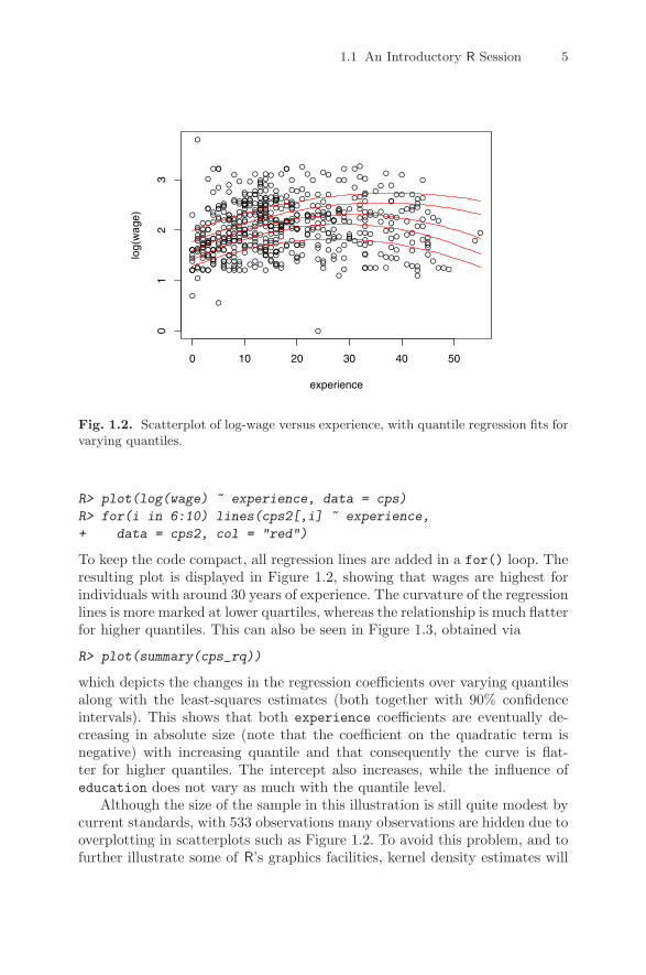
Fig. 1.2. Scatterplot of log-wage versus experience, with quantile regression fits forvarying quantiles.

R> plot(log(wage) ~ experience, data = cps)

R> for(i in 6:10) lines(cps2[,i] ~ experience,

+ data = cps2, col = "red")

To keep the code compact, all regression lines are added in a for() loop. Theresulting plot is displayed in Figure 1.2, showing that wages are highest forindividuals with around 30 years of experience. The curvature of the regressionlines is more marked at lower quartiles, whereas the relationship is much flatterfor higher quantiles. This can also be seen in Figure 1.3, obtained via

R> plot(summary(cps_rq))

which depicts the changes in the regression coefficients over varying quantilesalong with the least-squares estimates (both together with 90% confidenceintervals). This shows that both experience coefficients are eventually de-creasing in absolute size (note that the coefficient on the quadratic term isnegative) with increasing quantile and that consequently the curve is flat-ter for higher quantiles. The intercept also increases, while the influence ofeducation does not vary as much with the quantile level.

Although the size of the sample in this illustration is still quite modest bycurrent standards, with 533 observations many observations are hidden due tooverplotting in scatterplots such as Figure 1.2. To avoid this problem, and tofurther illustrate some of R’s graphics facilities, kernel density estimates will

0 10 20 30 40 50

01

23

experience

log(

wag

e)

6 1 Introduction

Fig. 1.3. Coefficients of quantile regression for varying quantiles, with confidencebands (gray) and least-squares estimate (red).

be used: high- versus low-density regions in the bivariate distribution can beidentified by a bivariate kernel density estimate and brought out graphicallyin a so-called heatmap. In R, the bivariate kernel density estimate is providedby bkde2D() in the package KernSmooth:

R> library("KernSmooth")

R> cps_bkde <- bkde2D(cbind(cps$experience, log(cps$wage)),

+ bandwidth = c(3.5, 0.5), gridsize = c(200, 200))

As bkde2D() does not have a formula interface (in contrast to lm() or rq()),we extract the relevant columns from the cps data set and select suitablebandwidths and grid sizes. The resulting 200×200 matrix of density estimates

0.2 0.3 0.4 0.5 0.6 0.7 0.8

0.0

0.2

0.4

0.6

0.8

(Intercept)

0.2 0.3 0.4 0.5 0.6 0.7 0.8

0.02

50.

035

0.04

50.

055

experience

0.2 0.3 0.4 0.5 0.6 0.7 0.8

−1e

−03

−8e

−04

−6e

−04

−4e

−04

I(experience^2)

0.2 0.3 0.4 0.5 0.6 0.7 0.8

0.05

0.07

0.09

0.11

education

1.1 An Introductory R Session 7

Fig. 1.4. Bivariate kernel density heatmap of log-wage by experience, with least-squares fit and prediction interval.

can be visualized in a heatmap using gray levels coding the density values.R provides image() (or contour()) to produce such displays, which can beapplied to cps_bkde as follows.

R> image(cps_bkde$x1, cps_bkde$x2, cps_bkde$fhat,

+ col = rev(gray.colors(10, gamma = 1)),

+ xlab = "experience", ylab = "log(wage)")

R> box()

R> lines(fit ~ experience, data = cps2)

R> lines(lwr ~ experience, data = cps2, lty = 2)

R> lines(upr ~ experience, data = cps2, lty = 2)

After drawing the heatmap itself, we add the regression line for the linearmodel fit along with prediction intervals (see Figure 1.4). Compared with thescatterplot in Figure 1.2, this brings out more clearly the empirical relationshipbetween log(wage) and experience.

This concludes our introductory R session. More details on the data sets,models, and R functions are provided in the following chapters.

0 10 20 30 40 50 60

01

23

4

experience

log(

wag

e)

8 1 Introduction

1.2 Getting Started

The R system for statistical computing and graphics (R Development CoreTeam 2008b, http://www.R-project.org/) is an open-source softwareproject, released under the terms of the GNU General Public License (GPL),Version 2. (Readers unfamiliar with open-source software may want to visithttp://www.gnu.org/.) Its source code as well as several binary versions canbe obtained, at no cost, from the Comprehensive R Archive Network (CRAN;see http://CRAN.R-project.org/mirrors.html to find its nearest mirrorsite). Binary versions are provided for 32-bit versions of Microsoft Windows,various flavors of Linux (including Debian, Red Hat, SUSE, and Ubuntu) andMac OS X.

Installation

Installation of binary versions is fairly straightforward: just go to CRAN, pickthe version corresponding to your operating system, and follow the instruc-tions provided in the corresponding readme file. For Microsoft Windows, thisamounts to downloading and running the setup executable (.exe file), whichtakes the user through a standard setup manager. For Mac OS X, separatedisk image .dmg files are available for the base system as well as for a GUIdeveloped for this platform. For various Linux flavors, there are prepackagedbinaries (as .rpm or .deb files) that can be installed with the usual pack-aging tools on the respective platforms. Additionally, versions of R are alsodistributed in many of the standard Linux repositories, although these are notnecessarily as quickly updated to new R versions as CRAN is.

For every system, in particular those for which a binary package does notexist, there is of course also the option to compile R from the source. Onsome platforms, notably Microsoft Windows, this can be a bit cumbersomebecause the required compilers are typically not part of a standard installation.On other platforms, such as Unix or Linux, this often just amounts to theusual configure/make/install steps. See R Development Core Team (2008d)for detailed information on installation and administration of R.

Packages

As will be discussed in greater detail below, base R is extended by meansof packages, some of which are part of the default installation. Packages arestored in one or more libraries (i.e., collections of packages) on the system andcan be loaded using the command library(). Typing library() without anyarguments returns a list of all currently installed packages in all libraries. Inthe R world, some of these are referred to as “base” packages (contained inthe R sources); others are “recommended” packages (included in every binarydistribution). A large number of further packages, known as “contributed”packages (currently more than 1,400), are available from the CRAN servers(see http://CRAN.R-project.org/web/packages/), and some of these will

1.3 Working with R 9

be required as we proceed. Notably, the package accompanying this book,named AER, is needed. On a computer connected to the Internet, its instal-lation is as simple as typing

R> install.packages("AER")

at the prompt. This installation process works on all operating systems; inaddition, Windows users may install packages by using the “Install packagesfrom CRAN”and Mac users by using the “Package installer”menu option andthen choosing the packages to be installed from a list. Depending on the instal-lation, in particular on the settings of the library paths, install.packages()by default might try to install a package in a directory where the user hasno writing permission. In such a case, one needs to specify the lib argumentor set the library paths appropriately (see R Development Core Team 2008d,and ?library for more information). Incidentally, installing AER will down-load several further packages on which AER depends. It is not uncommon forpackages to depend on other packages; if this is the case, the package “knows”about it and ensures that all the functions it depends upon will become avail-able during the installation process.

To use functions or data sets from a package, the package must be loaded.The command is, for our package AER,

R> library("AER")

From now on, we assume that AER is always loaded. It will be necessaryto install and load further packages in later chapters, and it will always beindicated what they are.

In view of the rapidly increasing number of contributed packages, ithas proven to be helpful to maintain a number of “CRAN task views”that provide an overview of packages for certain tasks. Current task viewsinclude econometrics, finance, social sciences, and Bayesian statistics. Seehttp://CRAN.R-project.org/web/views/ for further details.

1.3 Working with R

There is an important difference in philosophy between R and most othereconometrics packages. With many packages, an analysis will lead to a largeamount of output containing information on estimation, model diagnostics,specification tests, etc. In R, an analysis is normally broken down into a seriesof steps. Intermediate results are stored in objects, with minimal output ateach step (often none). Instead, the objects are further manipulated to obtainthe information required.

In fact, the fundamental design principle underlying R (and S) is “every-thing is an object”. Hence, not only vectors and matrices are objects thatcan be passed to and returned by functions, but also functions themselves,and even function calls. This enables computations on the language and canconsiderably facilitate programming tasks, as we will illustrate in Chapter 7.

10 1 Introduction

Handling objects

To see what objects are currently defined, the function objects() (or equiv-alently ls()) can be used. By default, it lists all objects in the global envi-ronment (i.e., the user’s workspace):

R> objects()

[1] "CPS1985" "Journals" "cps" "cps2" "cps_bkde"[6] "cps_lm" "cps_rq" "i" "j_lm"

which returns a character vector of length 9 telling us that there are currentlynine objects, resulting from the introductory session.

However, this cannot be the complete list of available objects, given thatsome objects must already exist prior to the execution of any commands,among them the function objects() that we just called. The reason is thatthe search list, which can be queried by

R> search()

[1] ".GlobalEnv" "package:KernSmooth"[3] "package:quantreg" "package:SparseM"[5] "package:AER" "package:survival"[7] "package:splines" "package:strucchange"[9] "package:sandwich" "package:lmtest"[11] "package:zoo" "package:car"[13] "package:stats" "package:graphics"[15] "package:grDevices" "package:utils"[17] "package:datasets" "package:methods"[19] "Autoloads" "package:base"

comprises not only the global environment ".GlobalEnv" (always at the firstposition) but also several attached packages, including the base package at itsend. Calling objects("package:base") will show the names of more than athousand objects defined in base, including the function objects() itself.

Objects can easily be created by assigning a value to a name using theassignment operator <-. For illustration, we create a vector x in which thenumber 2 is stored:

R> x <- 2

R> objects()

[1] "CPS1985" "Journals" "cps" "cps2" "cps_bkde"[6] "cps_lm" "cps_rq" "i" "j_lm" "x"

x is now available in our global environment and can be removed using thefunction remove() (or equivalently rm()):

R> remove(x)

R> objects()

1.3 Working with R 11

[1] "CPS1985" "Journals" "cps" "cps2" "cps_bkde"[6] "cps_lm" "cps_rq" "i" "j_lm"

Calling functions

If the name of an object is typed at the prompt, it will be printed. For afunction, say foo, this means that the corresponding R source code is printed(try, for example, objects), whereas if it is called with parentheses, as infoo(), it is a function call. If there are no arguments to the function, or allarguments have defaults (as is the case with objects()), then foo() is avalid function call. Therefore, a pair of parentheses following the object nameis employed throughout this book to signal that the object discussed is afunction.

Functions often have more than one argument (in fact, there is no limitto the number of arguments to R functions). A function call may use thearguments in any order, provided the name of the argument is given. If namesof arguments are not given, R assumes they appear in the order of the functiondefinition. If an argument has a default, it may be left out in a function call.For example, the function log() has two arguments, x and base: the first, x,can be a scalar (actually also a vector), the logarithm of which is to be taken;the second, base, is the base with respect to which logarithms are computed.

Thus, the following four calls are all equivalent:

R> log(16, 2)

R> log(x = 16, 2)

R> log(16, base = 2)

R> log(base = 2, x = 16)

Classes and generic functions

Every object has a class that can be queried using class(). Classes include“data.frame” (a list or array with a certain structure, the preferred formatin which data should be held), “lm” for linear-model objects (returned whenfitting a linear regression model by ordinary least squares; see Section 1.1above), and “matrix” (which is what the name suggests). For each class, cer-tain methods to so-called generic functions are available; typical examplesinclude summary() and plot(). The result of these functions depends on theclass of the object: when provided with a numerical vector, summary() re-turns basic summaries of an empirical distribution, such as the mean and themedian; for a vector of categorical data, it returns a frequency table; and inthe case of a linear-model object, the result is the standard regression out-put. Similarly, plot() returns pairs of scatterplots when provided with a dataframe and returns basic diagnostic plots for a linear-model object.

12 1 Introduction

Quitting R

One exits R by using the q() function:

R> q()

R will then ask whether to save the workspace image. Answering n (no) willexit R without saving anything, whereas answering y (yes) will save all cur-rently defined objects in a file .RData and the command history in a file.Rhistory, both in the working directory.

File management

To query the working directory, use getwd(), and to change it, setwd(). Ifan R session is started in a directory that has .RData and/or .Rhistory files,these will automatically be loaded. Saved workspaces from other directoriescan be loaded using the function load(). Analogously, R objects can be saved(in binary format) by save(). To query the files in a directory, dir() can beused.

1.4 Getting Help

R is well-documented software. Help on any function may be accessed usingeither ? or help(). Thus

R> ?options

R> help("options")

both open the help page for the command options(). At the bottom ofa help page, there are typically practical examples of how to use thatfunction. These can easily be executed with the example() function; e.g.,example("options") or example("lm").

If the exact name of a command is not known, as will often be thecase for beginners, the functions to use are help.search() and apropos().help.search() returns help files with aliases or concepts or titles matching a“pattern”using fuzzy matching. Thus, if help on options settings is desired butthe exact command name, here options(), is unknown, a search for objectscontaining the pattern“option”might be useful. help.search("option") willreturn a (long) list of commands, data frames, etc., containing this pattern,including an entry

options(base) Options Settings

providing the desired result. It says that there exists a command options()in the base package that provides options settings.

Alternatively, the function apropos() lists all functions whose names in-clude the pattern entered. As an illustration,

1.4 Getting Help 13

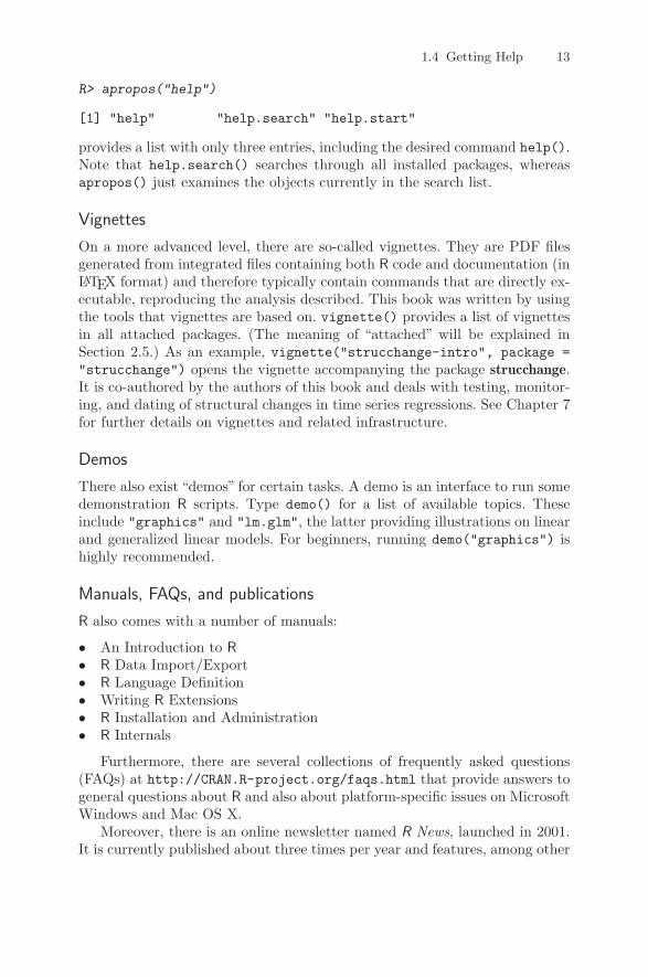
R> apropos("help")

[1] "help" "help.search" "help.start"

provides a list with only three entries, including the desired command help().Note that help.search() searches through all installed packages, whereasapropos() just examines the objects currently in the search list.

Vignettes

On a more advanced level, there are so-called vignettes. They are PDF filesgenerated from integrated files containing both R code and documentation (inLATEX format) and therefore typically contain commands that are directly ex-ecutable, reproducing the analysis described. This book was written by usingthe tools that vignettes are based on. vignette() provides a list of vignettesin all attached packages. (The meaning of “attached” will be explained inSection 2.5.) As an example, vignette("strucchange-intro", package ="strucchange") opens the vignette accompanying the package strucchange.It is co-authored by the authors of this book and deals with testing, monitor-ing, and dating of structural changes in time series regressions. See Chapter 7for further details on vignettes and related infrastructure.

Demos

There also exist “demos” for certain tasks. A demo is an interface to run somedemonstration R scripts. Type demo() for a list of available topics. Theseinclude "graphics" and "lm.glm", the latter providing illustrations on linearand generalized linear models. For beginners, running demo("graphics") ishighly recommended.

Manuals, FAQs, and publications

R also comes with a number of manuals:

• An Introduction to R• R Data Import/Export• R Language Definition• Writing R Extensions• R Installation and Administration• R Internals

Furthermore, there are several collections of frequently asked questions(FAQs) at http://CRAN.R-project.org/faqs.html that provide answers togeneral questions about R and also about platform-specific issues on MicrosoftWindows and Mac OS X.

Moreover, there is an online newsletter named R News, launched in 2001.It is currently published about three times per year and features, among other

14 1 Introduction

things, recent developments in R (such as changes in the language or new add-on packages), a “programmer’s niche”, and examples analyzing data with R.See http://CRAN.R-project.org/doc/Rnews/ for further information.

For a growing number of R packages, there exist corresponding publica-tions in the Journal of Statistical Software; see http://www.jstatsoft.org/.This is an open-access journal that publishes articles and code snippets (aswell as book and software reviews) on the subject of statistical software andalgorithms. A special volume on Econometrics in R is currently in preparation.

Finally, there is a rapidly growing list of books on R, or on statistics usingR, at all levels, the most comprehensive perhaps being Venables and Ripley(2002). In addition, we refer the interested reader to Dalgaard (2002) forintroductory statistics, to Murrell (2005) for R graphics, and to Faraway (2005)for linear regression.

1.5 The Development Model

One of R’s strengths and a key feature in its success is that it is highly ex-tensible through packages that can provide extensions to everything availablein the base system. This includes not only R code but also code in compiledlanguages (such as C, C++, or FORTRAN), data sets, demo files, test suites, vi-gnettes, or further documentation. Therefore, every R user can easily becomean R developer by submitting his or her packages to CRAN to share themwith the R community. Hence packages can actively influence the direction inwhich (parts of) R will go in the future.

Unlike the CRAN packages, the base R system is maintained and developedonly by the R core team, which releases major version updates (i.e., versionsx.y.0) biannually (currently around April 1 and October 1). However, as Ris an open-source system, all users are given read access to the master SVNrepository—SVN stands for Subversion and is a version control system; seehttp://subversion.tigris.org/—and can thus check out the full sourcecode of the development version of R.

In addition, there are several means of communication within the R userand developer community and between the users and the core developmentteam. The two most important are various R mailing lists and, as describedabove, CRAN packages. The R project hosts several mailing lists, includingR-help and R-devel. The former can be used to ask for help on using R, thelatter for discussing issues related to the development of R or R packages.Furthermore, bugs can be reported and feature requests made. The postingguide at http://www.R-project.org/posting-guide.html discusses somegood strategies for doing this effectively. In addition to these general mailinglists, there are lists for special interest groups (SIGs), among them at leastone list that might be of interest to the reader: it is devoted to finance and(financial) econometrics and is called R-SIG-Finance.

1.6 A Brief History of R 15

1.6 A Brief History of R

As noted above, the R system for statistical computing and graphics (R Devel-opment Core Team 2008b, http://www.R-project.org/) is an open-sourcesoftware project. The story begins at Bell Laboratories (of AT&T and nowAlcatel-Lucent in New Jersey), with the S language, a system for data anal-ysis developed by John Chambers, Rick Becker, and collaborators since thelate 1970s. Landmarks of the development of S are a series of books, referredto by color in the S community, beginning with the “brown book” (Beckerand Chambers 1984), which features “Old S”. The basic reference for “NewS”, or S version 2, is Becker, Chambers, and Wilks (1988), the “blue book”.For S version 3 (first-generation object-oriented programming and statisticalmodeling), it is Chambers and Hastie (1992), the “white book”. The “greenbook” (Chambers 1998) documents S version 4. Based on the various S ver-sions, Insightful Corporation (formerly MathSoft and still earlier StatisticalSciences) has provided a commercially enhanced and supported release of S,named S-PLUS, since 1987. At its core, this includes the original S imple-mentation, which was first exclusively licensed and finally purchased in 2004.On March 23, 1999, the Association for Computing Machinery (ACM) namedJohn Chambers as the recipient of its 1998 Software System Award for de-veloping the S system, noting that his work “will forever alter the way peopleanalyze, visualize, and manipulate data”.

R itself was initially developed by Robert Gentleman and Ross Ihaka at theUniversity of Auckland, New Zealand. An early version is described in an arti-cle by its inventors (Ihaka and Gentleman 1996). They designed the languageto combine the strengths of two existing languages, S and Scheme (Steel andSussman 1975). In the words of Ihaka and Gentleman (1996), “[t]he resultinglanguage is very similar in appearance to S, but the underlying implementa-tion and semantics are derived from Scheme”. The result was baptized R “inpart to acknowledge the influence of S and in part to celebrate [their] ownefforts”.

The R source code was first released under the GNU General Public Li-cense (GPL) in 1995. Since mid-1997, there has been the R Development CoreTeam, currently comprising 19 members, and their names are available upontyping contributors() in an R session. In 1998, the Comprehensive R ArchiveNetwork (CRAN; http://CRAN.R-project.org/) was established, which isa family of mirror sites around the world that store identical, up-to-date ver-sions of code and documentation for R. The first official release, R version1.0.0, dates to 2000-02-29. It implements the S3 standard as documented byChambers and Hastie (1992). R version 2.0.0 was released in 2004, and thecurrent version of the language, R 2.7.0, may be viewed as implementing S4(Chambers 1998) plus numerous concepts that go beyond the various S stan-dards.

The first publication on R in the econometrics literature appears to havebeen by Cribari-Neto and Zarkos (1999), a software review in the Journal

16 1 Introduction

of Applied Econometrics entitled “R: Yet Another Econometric ProgrammingEnvironment”. It describes R version 0.63.1, still a beta version. Three yearslater, in a further software review in the same journal, Racine and Hynd-man (2002) focused on using R for teaching econometrics utilizing R 1.3.1.To the best of our knowledge, this book is the first general introduction toeconometric computing with R.

2

Basics

R can be used at various levels. Of course, standard arithmetic is available,and hence it can be used as a (rather sophisticated) calculator. It is alsoprovided with a graphical system that writes on a large variety of devices.Furthermore, R is a full-featured programming language that can be employedto tackle all typical tasks for which other programming languages are alsoused. It connects to other languages, programs, and data bases, and also tothe operating system; users can control all these from within R.

In this chapter, we illustrate a few of the typical uses of R. Often solutionsare not unique, but in the following we avoid sophisticated shortcuts. However,we encourage all readers to explore alternative solutions by reusing what theyhave learned in other contexts.

2.1 R as a Calculator

The standard arithmetic operators +, -, *, /, and ^ are available, wherex^y yields xy. Hence

R> 1 + 1

[1] 2

R> 2^3

[1] 8

In the output, [1] indicates the position of the first element of the vectorreturned by R. This is not surprising here, where all vectors are of length 1,but it will be useful later.

The common mathematical functions, such as log(), exp(), sin(),asin(), cos(), acos(), tan(), atan(), sign(), sqrt(), abs(), min(), andmax(), are also available. Specifically, log(x, base = a) returns the loga-rithm of x to base a, where a defaults to exp(1). Thus

C. Kleiber, A. Zeileis, Applied Econometrics with R,DOI: 10.1007/978-0-387-77318-6 2, © Springer Science+Business Media, LLC 2008

18 2 Basics

R> log(exp(sin(pi/4)^2) * exp(cos(pi/4)^2))

[1] 1

which also shows that pi is a built-in constant. There are further conve-nience functions, such as log10() and log2(), but here we shall mainly uselog(). A full list of all options and related functions is available upon typing?log, ?sin, etc. Additional functions useful in statistics and econometrics aregamma(), beta(), and their logarithms and derivatives. See ?gamma for furtherinformation.

Vector arithmetic

In R, the basic unit is a vector, and hence all these functions operate directlyon vectors. A vector is generated using the function c(), where c stands for“combine” or “concatenate”. Thus

R> x <- c(1.8, 3.14, 4, 88.169, 13)

generates an object x, a vector, containing the entries 1.8, 3.14, 4, 88.169,13. The length of a vector is available using length(); thus

R> length(x)

[1] 5

Note that names are case-sensitive; hence x and X are distinct.The preceding statement uses the assignment operator <-, which should

be read as a single symbol (although it requires two keystrokes), an arrowpointing to the variable to which the value is assigned. Alternatively, = maybe used at the user level, but since <- is preferred for programming, it is usedthroughout this book. There is no immediately visible result, but from nowon x has as its value the vector defined above, and hence it can be used insubsequent computations:

R> 2 * x + 3

[1] 6.60 9.28 11.00 179.34 29.00

R> 5:1 * x + 1:5

[1] 10.00 14.56 15.00 180.34 18.00

This requires an explanation. In the first statement, the scalars (i.e., vec-tors of length 1) 2 and 3 are recycled to the length of x so that each element ofx is multiplied by 2 before 3 is added. In the second statement, x is multipliedelement-wise by the vector 1:5 (the sequence from 1 to 5; see below) and thenthe vector 5:1 is added element-wise.

Mathematical functions can be applied as well; thus

R> log(x)

2.1 R as a Calculator 19

[1] 0.5878 1.1442 1.3863 4.4793 2.5649

returns a vector containing the logarithms of the original entries of x.

Subsetting vectors

It is often necessary to access subsets of vectors. This requires the operator[, which can be used in several ways to extract elements of a vector. Forexample, one can either specify which elements to include or which elementsto exclude: a vector of positive indices, such as

R> x[c(1, 4)]

[1] 1.80 88.17

specifies the elements to be extracted. Alternatively, a vector of negative in-dices, as in

R> x[-c(2, 3, 5)]

[1] 1.80 88.17

selects all elements but those indicated, yielding the same result. In fact,further methods are available for subsetting with [, which are explained below.

Patterned vectors

In statistics and econometrics, there are many instances where vectors withspecial patterns are needed. R provides a number of functions for creatingsuch vectors, including

R> ones <- rep(1, 10)

R> even <- seq(from = 2, to = 20, by = 2)

R> trend <- 1981:2005

Here, ones is a vector of ones of length 10, even is a vector containing theeven numbers from 2 to 20, and trend is a vector containing the integers from1981 to 2005.

Since the basic element is a vector, it is also possible to concatenate vectors.Thus

R> c(ones, even)

[1] 1 1 1 1 1 1 1 1 1 1 2 4 6 8 10 12 14 16 18 20

creates a vector of length 20 consisting of the previously defined vectors onesand even laid end to end.

20 2 Basics

2.2 Matrix Operations

A 2× 3 matrix containing the elements 1:6, by column, is generated via

R> A <- matrix(1:6, nrow = 2)

Alternatively, ncol could have been used, with matrix(1:6, ncol = 3)yielding the same result.

Basic matrix algebra

The transpose A> of A is

R> t(A)

[,1] [,2][1,] 1 2[2,] 3 4[3,] 5 6

The dimensions of a matrix may be accessed using dim(), nrow(), and ncol();hence

R> dim(A)

[1] 2 3

R> nrow(A)

[1] 2

R> ncol(A)

[1] 3

Single elements of a matrix, row or column vectors, or indeed entire sub-matrices may be extracted by specifying the rows and columns of the matrixfrom which they are selected. This uses a simple extension of the rules forsubsetting vectors. (In fact, internally, matrices are vectors with an additionaldimension attribute enabling row/column-type indexing.) Element aij of amatrix A is extracted using A[i,j]. Entire rows or columns can be extractedvia A[i,] and A[,j], respectively, which return the corresponding row orcolumn vectors. This means that the dimension attribute is dropped (by de-fault); hence subsetting will return a vector instead of a matrix if the resultingmatrix has only one column or row. Occasionally, it is necessary to extractrows, columns, or even single elements of a matrix as a matrix. Dropping ofthe dimension attribute can be switched off using A[i, j, drop = FALSE].As an example,

R> A1 <- A[1:2, c(1, 3)]

2.2 Matrix Operations 21

selects a square matrix containing the first and third elements from each row(note that A has only two rows in our example). Alternatively, and morecompactly, A1 could have been generated using A[, -2]. If no row numberis specified, all rows will be taken; the -2 specifies that all columns but thesecond are required.

A1 is a square matrix, and if it is nonsingular it has an inverse. One wayto check for singularity is to compute the determinant using the R functiondet(). Here, det(A1) equals −4; hence A1 is nonsingular. Alternatively, itseigenvalues (and eigenvectors) are available using eigen(). Here, eigen(A1)yields the eigenvalues 7.531 and −0.531, again showing that A1 is nonsingular.

The inverse of a matrix, if it cannot be avoided, is computed using solve():

R> solve(A1)

[,1] [,2][1,] -1.5 1.25[2,] 0.5 -0.25

We can check that this is indeed the inverse of A1 by multiplying A1 with itsinverse. This requires the operator for matrix multiplication, %*%:

R> A1 %*% solve(A1)

[,1] [,2][1,] 1 0[2,] 0 1

Similarly, conformable matrices are added and subtracted using the arith-metical operators + and -. It is worth noting that for non-conformable matricesrecycling proceeds along columns. Incidentally, the operator * also works formatrices; it returns the element-wise or Hadamard product of conformablematrices. Further types of matrix products that are often required in econo-metrics are the Kronecker product, available via kronecker(), and the crossproduct A>B of two matrices, for which a computationally efficient algorithmis implemented in crossprod().

In addition to the spectral decomposition computed by eigen() as men-tioned above, R provides other frequently used matrix decompositions, includ-ing the singular-value decomposition svd(), the QR decomposition qr(), andthe Cholesky decomposition chol().

Patterned matrices

In econometrics, there are many instances where matrices with special pat-terns occur. R provides functions for generating matrices with such patterns.For example, a diagonal matrix with ones on the diagonal may be createdusing

R> diag(4)

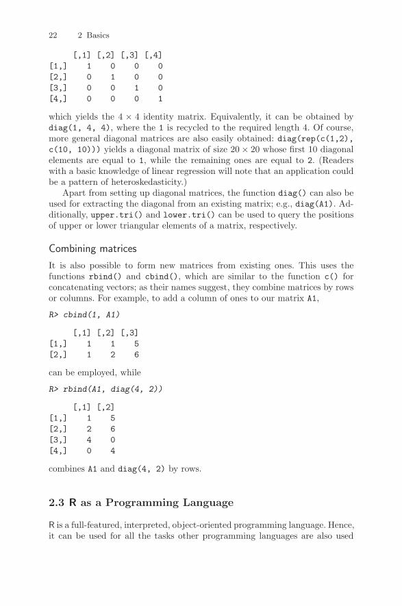
22 2 Basics

[,1] [,2] [,3] [,4][1,] 1 0 0 0[2,] 0 1 0 0[3,] 0 0 1 0[4,] 0 0 0 1

which yields the 4 × 4 identity matrix. Equivalently, it can be obtained bydiag(1, 4, 4), where the 1 is recycled to the required length 4. Of course,more general diagonal matrices are also easily obtained: diag(rep(c(1,2),c(10, 10))) yields a diagonal matrix of size 20× 20 whose first 10 diagonalelements are equal to 1, while the remaining ones are equal to 2. (Readerswith a basic knowledge of linear regression will note that an application couldbe a pattern of heteroskedasticity.)

Apart from setting up diagonal matrices, the function diag() can also beused for extracting the diagonal from an existing matrix; e.g., diag(A1). Ad-ditionally, upper.tri() and lower.tri() can be used to query the positionsof upper or lower triangular elements of a matrix, respectively.

Combining matrices

It is also possible to form new matrices from existing ones. This uses thefunctions rbind() and cbind(), which are similar to the function c() forconcatenating vectors; as their names suggest, they combine matrices by rowsor columns. For example, to add a column of ones to our matrix A1,

R> cbind(1, A1)

[,1] [,2] [,3][1,] 1 1 5[2,] 1 2 6

can be employed, while

R> rbind(A1, diag(4, 2))

[,1] [,2][1,] 1 5[2,] 2 6[3,] 4 0[4,] 0 4

combines A1 and diag(4, 2) by rows.

2.3 R as a Programming Language

R is a full-featured, interpreted, object-oriented programming language. Hence,it can be used for all the tasks other programming languages are also used

2.3 R as a Programming Language 23

for, not only for data analysis. What makes it particularly useful for statis-tics and econometrics is that it was designed for “programming with data”(Chambers 1998). This has several implications for the data types employedand the object-orientation paradigm used (see Section 2.6 for more on objectorientation).

An in-depth treatment of programming in S/R is given in Venables andRipley (2000). If you read German, Ligges (2007) is an excellent introductionto programming with R. On a more advanced level, R Development Core Team(2008f,g) provides guidance about the language definition and how extensionsto the R system can be written. The latter documents can be downloadedfrom CRAN and also ship with every distribution of R.

The mode of a vector

Probably the simplest data structure in R is a vector. All elements of a vectormust be of the same type; technically, they must be of the same “mode”. Themode of a vector x can be queried using mode(x). Here, we need vectors ofmodes “numeric”, “logical”, and “character” (but there are others).

We have already seen that

R> x <- c(1.8, 3.14, 4, 88.169, 13)

creates a numerical vector, and one typical application of vectors is to storethe values of some numerical variable in a data set.

Logical and character vectors

Logical vectors may contain the logical constants TRUE and FALSE. In a freshsession, the aliases T and F are also available for compatibility with S (whichuses these as the logical constants). However, unlike TRUE and FALSE, thevalues of T and F can be changed (e.g., by using the former for signifying thesample size in a time series context or using the latter as the variable for anF statistic), and hence it is recommended not to rely on them but to alwaysuse TRUE and FALSE. Like numerical vectors, logical vectors can be createdfrom scratch. They may also arise as the result of a logical comparison:

R> x > 3.5

[1] FALSE FALSE TRUE TRUE TRUE

Further logical operations are explained below.Character vectors can be employed to store strings. Especially in the early

chapters of this book, we will mainly use them to assign labels or namesto certain objects such as vectors and matrices. For example, we can assignnames to the elements of x via

R> names(x) <- c("a", "b", "c", "d", "e")

R> x

24 2 Basics

a b c d e1.80 3.14 4.00 88.17 13.00

Alternatively, we could have used names(x) <- letters[1:5] since lettersand LETTERS are built-in vectors containing the 26 lower- and uppercase lettersof the Latin alphabet, respectively. Although we do not make much use of themin this book, we note here that the character-manipulation facilities of R go farbeyond these simple examples, allowing, among other things, computations ontext documents or command strings.

More on subsetting

Having introduced vectors of modes numeric, character, and logical, it is usefulto revisit subsetting of vectors. By now, we have seen how to extract partsof a vector using numerical indices, but in fact this is also possible usingcharacters (if there is a names attribute) or logicals (in which case the elementscorresponding to TRUE are selected). Hence, the following commands yield thesame result:

R> x[3:5]

c d e4.00 88.17 13.00

R> x[c("c", "d", "e")]

c d e4.00 88.17 13.00

R> x[x > 3.5]

c d e4.00 88.17 13.00

Subsetting of matrices (and also of data frames or multidimensional arrays)works similarly.

Lists

So far, we have only used plain vectors. We now proceed to introduce somerelated data structures that are similar but contain more information.

In R, lists are generic vectors where each element can be virtually any typeof object; e.g., a vector (of arbitrary mode), a matrix, a full data frame, afunction, or again a list. Note that the latter also allows us to create recursivedata structures. Due to this flexibility, lists are the basis for most complexobjects in R; e.g., for data frames or fitted regression models (to name twoexamples that will be described later).

As a simple example, we create, using the function list(), a list containinga sample from a standard normal distribution (generated with rnorm(); see

2.3 R as a Programming Language 25

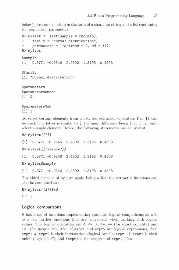
below) plus some markup in the form of a character string and a list containingthe population parameters.

R> mylist <- list(sample = rnorm(5),

+ family = "normal distribution",

+ parameters = list(mean = 0, sd = 1))

R> mylist

$sample[1] 0.3771 -0.9346 2.4302 1.3195 0.4503

$family[1] "normal distribution"

$parameters$parameters$mean[1] 0

$parameters$sd[1] 1

To select certain elements from a list, the extraction operators $ or [[ canbe used. The latter is similar to [, the main difference being that it can onlyselect a single element. Hence, the following statements are equivalent:

R> mylist[[1]]

[1] 0.3771 -0.9346 2.4302 1.3195 0.4503

R> mylist[["sample"]]

[1] 0.3771 -0.9346 2.4302 1.3195 0.4503

R> mylist$sample

[1] 0.3771 -0.9346 2.4302 1.3195 0.4503

The third element of mylist again being a list, the extractor functions canalso be combined as in

R> mylist[[3]]$sd

[1] 1

Logical comparisons

R has a set of functions implementing standard logical comparisons as wellas a few further functions that are convenient when working with logicalvalues. The logical operators are <, <=, >, >=, == (for exact equality) and!= (for inequality). Also, if expr1 and expr2 are logical expressions, thenexpr1 & expr2 is their intersection (logical “and”), expr1 | expr2 is theirunion (logical “or”), and !expr1 is the negation of expr1. Thus

26 2 Basics

R> x <- c(1.8, 3.14, 4, 88.169, 13)

R> x > 3 & x <= 4

[1] FALSE TRUE TRUE FALSE FALSE

To assess for which elements of a vector a certain expression is TRUE, thefunction which() can be used:

R> which(x > 3 & x <= 4)

[1] 2 3

The specialized functions which.min() and which.max() are available forcomputing the position of the minimum and the maximum. In addition to& and |, the functions all() and any() check whether all or at least someentries of a vector are TRUE:

R> all(x > 3)

[1] FALSE

R> any(x > 3)

[1] TRUE

Some caution is needed when assessing exact equality. When applied to nu-merical input, == does not allow for finite representation of fractions or forrounding error; hence situations like

R> (1.5 - 0.5) == 1

[1] TRUE

R> (1.9 - 0.9) == 1

[1] FALSE

can occur due to floating-point arithmetic (Goldberg 1991). For these pur-poses, all.equal() is preferred:

R> all.equal(1.9 - 0.9, 1)

[1] TRUE

Furthermore, the function identical() checks whether two R objects areexactly identical.

Due to coercion, it is also possible to compute directly on logical vectorsusing ordinary arithmetic. When coerced to numeric, FALSE becomes 0 andTRUE becomes 1, as in

R> 7 + TRUE

[1] 8

2.3 R as a Programming Language 27

Coercion

To convert an object from one type or class to a different one, R provides anumber of coercion functions, conventionally named as.foo(), where foo isthe desired type or class; e.g., numeric, character, matrix, and data.frame(a concept introduced in Section 2.5), among many others. They are typicallyaccompanied by an is.foo() function that checks whether an object is of typeor class foo. Thus

R> is.numeric(x)

[1] TRUE

R> is.character(x)

[1] FALSE

R> as.character(x)

[1] "1.8" "3.14" "4" "88.169" "13"

In certain situations, coercion is also forced automatically by R; e.g., whenthe user tries to put elements of different modes into a single vector (whichcan only contain elements of the same mode). Thus

R> c(1, "a")

[1] "1" "a"

Random number generation

For programming environments in statistics and econometrics, it is vital tohave good random number generators (RNGs) available, in particular to allowthe users to carry out Monte Carlo studies. The R RNG supports severalalgorithms; see ?RNG for further details. Here, we outline a few importantcommands.

The RNG relies on a “random seed”, which is the basis for the genera-tion of pseudo-random numbers. By setting the seed to a specific value usingthe function set.seed(), simulations can be made exactly reproducible. Forexample, using the function rnorm() for generating normal random numbers,

R> set.seed(123)

R> rnorm(2)

[1] -0.5605 -0.2302

R> rnorm(2)

[1] 1.55871 0.07051

R> set.seed(123)

R> rnorm(2)

28 2 Basics

[1] -0.5605 -0.2302

Another basic function for drawing random samples, with or without replace-ment from a finite set of values, is sample(). The default is to draw, withoutreplacement, a vector of the same size as its input argument; i.e., to computea permutation of the input as in

R> sample(1:5)

[1] 5 1 2 3 4

R> sample(c("male", "female"), size = 5, replace = TRUE,

+ prob = c(0.2, 0.8))

[1] "female" "male" "female" "female" "female"

The second command draws a sample of size 5, with replacement, from thevalues "male" and "female", which are drawn with probabilities 0.2 and 0.8,respectively.

Above, we have already used the function rnorm() for drawing from anormal distribution. It belongs to a broader family of functions that are all ofthe form rdist(), where dist can be, for example, norm, unif, binom, pois, t,f, chisq, corresponding to the obvious families of distributions. All of thesefunctions take the sample size n as their first argument along with furtherarguments controlling parameters of the respective distribution. For exam-ple, rnorm() takes mean and sd as further arguments, with 0 and 1 beingthe corresponding defaults. However, these are not the only functions avail-able for statistical distributions. Typically there also exist ddist(), pdist(),and qdist(), which implement the density, cumulative probability distributionfunction, and quantile function (inverse distribution function), respectively.

Flow control

Like most programming languages, R provides standard control structuressuch as if/else statements, for loops, and while loops. All of these have incommon that an expression expr is evaluated, either conditional upon a cer-tain condition cond (for if and while) or for a sequence of values (for for).The expression expr itself can be either a simple expression or a compound ex-pression; i.e., typically a set of simple expressions enclosed in braces ... .Below we present a few brief examples illustrating its use; see ?Control forfurther information.

An if/else statement is of the form

if(cond)

expr1

else

expr2

2.3 R as a Programming Language 29

where expr1 is evaluated if cond is TRUE and expr2 otherwise. The elsebranch may be omitted if empty. A simple (if not very meaningful) exampleis

R> x <- c(1.8, 3.14, 4, 88.169, 13)

R> if(rnorm(1) > 0) sum(x) else mean(x)

[1] 22.02

where conditional on the value of a standard normal random number eitherthe sum or the mean of the vector x is computed. Note that the condition condcan only be of length 1. However, there is also a function ifelse() offering avectorized version; e.g.,

R> ifelse(x > 4, sqrt(x), x^2)

[1] 3.240 9.860 16.000 9.390 3.606

This computes the square root for those values in x that are greater than 4and the square for the remaining ones.

A for loop looks similar, but the main argument to for() is of typevariable in sequence. To illustrate its use, we recursively compute firstdifferences in the vector x.

R> for(i in 2:5)

+ x[i] <- x[i] - x[i-1]

+

R> x[-1]

[1] 1.34 2.66 85.51 -72.51

Finally, a while loop looks quite similar. The argument to while() is a con-dition that may change in every run of the loop so that it finally can becomeFALSE, as in

R> while(sum(x) < 100)

+ x <- 2 * x

+

R> x

[1] 14.40 10.72 21.28 684.07 -580.07

Writing functions

One of the features of S and R is that users naturally become developers.Creating variables or objects and applying functions to them interactively(either to modify them or to create other objects of interest) is part of everyR session. In doing so, typical sequences of commands often emerge that arecarried out for different sets of input values. Instead of repeating the samesteps “by hand”, they can also be easily wrapped into a function. A simpleexample is

30 2 Basics

R> cmeans <- function(X)

+ rval <- rep(0, ncol(X))

+ for(j in 1:ncol(X))

+ mysum <- 0

+ for(i in 1:nrow(X)) mysum <- mysum + X[i,j]

+ rval[j] <- mysum/nrow(X)

+

+ return(rval)

+

This creates a (deliberately awkward!) function cmeans(), which takes a ma-trix argument X and uses a double for loop to compute first the sum and thenthe mean in each column. The result is stored in a vector rval (our returnvalue), which is returned after both loops are completed. This function canthen be easily applied to new data, as in

R> X <- matrix(1:20, ncol = 2)

R> cmeans(X)

[1] 5.5 15.5

and (not surprisingly) yields the same result as the built-in functioncolMeans():

R> colMeans(X)

[1] 5.5 15.5

The function cmeans() takes only a single argument X that has no defaultvalue. If the author of a function wants to set a default, this can be easilyachieved by defining a function with a list of name = expr pairs, wherename is the argument of the variable and expr is an expression with thedefault value. If the latter is omitted, no default value is set.

In interpreted matrix-based languages such as R, loops are typically lessefficient than the corresponding vectorized computations offered by the sys-tem. Therefore, avoiding loops by replacing them with vectorized operationscan save computation time, especially when the number of iterations in theloop can become large. To illustrate, let us generate 2 · 106 random num-bers from the standard normal distribution and compare the built-in functioncolMeans() with our awkward function cmeans(). We employ the functionsystem.time(), which is useful for profiling code:

R> X <- matrix(rnorm(2*10^6), ncol = 2)

R> system.time(colMeans(X))

user system elapsed0.004 0.000 0.005

R> system.time(cmeans(X))

2.3 R as a Programming Language 31

user system elapsed5.572 0.004 5.617

Clearly, the performance of cmeans() is embarrassing, and using colMeans()is preferred.

Vectorized calculations

As noted above, loops can be avoided using vectorized arithmetic. In thecase of cmeans(), our function calculating column-wise means of a matrix,it would be helpful to directly compute means column by column using thebuilt-in function mean(). This is indeed the preferred solution. Using the toolsavailable to us thus far, we could proceed as follows:

R> cmeans2 <- function(X)

+ rval <- rep(0, ncol(X))

+ for(j in 1:ncol(X)) rval[j] <- mean(X[,j])

+ return(rval)

+

This eliminates one of the for loops and only cycles over the columns. Theresult is identical to the previous solutions, but the performance is clearlybetter than that of cmeans():

R> system.time(cmeans2(X))

user system elapsed0.072 0.008 0.080

However, the code of cmeans2() still looks a bit cumbersome with the re-maining for loop—it can be written much more compactly using the functionapply(). This applies functions over the margins of an array and takes threearguments: the array, the index of the margin, and the function to be evalu-ated. In our case, the function call is

R> apply(X, 2, mean)

because we require means (using mean()) over the columns (i.e., the seconddimension) of X. The performance of apply() can sometimes be better thana for loop; however, in many cases both approaches perform rather similarly:

R> system.time(apply(X, 2, mean))

user system elapsed0.084 0.028 0.114

To summarize, this means that (1) element-wise computations should beavoided if vectorized computations are available, (2) optimized solutions (ifavailable) typically perform better than the generic for or apply() solution,and (3) loops can be written more compactly using the apply() function. In

32 2 Basics

fact, this is so common in R that several variants of apply() are available,namely lapply(), tapply(), and sapply(). The first returns a list, the seconda table, and the third tries to simplify the result to a vector or matrix wherepossible. See the corresponding manual pages for more detailed informationand examples.

Reserved words

Like most programming languages, R has a number of reserved words thatprovide the basic grammatical constructs of the language. Some of these havealready been introduced above, and some more follow below. An almost com-plete list of reserved words in R is: if, else, for, in, while, repeat, break,next, function, TRUE, FALSE, NA, NULL, Inf, NaN, ...). See ?Reserved for acomplete list. If it is attempted to use any of these as names, this results inan error.

2.4 Formulas

Formulas are constructs used in various statistical programs for specifyingmodels. In R, formula objects can be used for storing symbolic descriptionsof relationships among variables, such as the ~ operator in the formation of aformula:

R> f <- y ~ x

R> class(f)

[1] "formula"

So far, this is only a description without any concrete meaning. The resultentirely depends on the function evaluating this formula. In R, the expressionabove commonly means “y is explained by x”. Such formula interfaces areconvenient for specifying, among other things, plots or regression relationships.For example, with

R> x <- seq(from = 0, to = 10, by = 0.5)

R> y <- 2 + 3 * x + rnorm(21)

the code

R> plot(y ~ x)

R> lm(y ~ x)

Call:lm(formula = y ~ x)

Coefficients:(Intercept) x

2.00 3.01

2.5 Data Management in R 33

Fig. 2.1. Simple scatterplot of y vs. x.

first generates a scatterplot of y against x (see Figure 2.1) and then fits thecorresponding simple linear regression model with slope 3.01 and intercept2.00.

For specifying regression models, the formula language is much richer thanoutlined above and is based on a symbolic notation suggested by Wilkinsonand Rogers (1973) in the statistical literature. For example, when using lm(),log(y) ~ x1 + x2 specifies a linear regression of log(y) on two regressorsx1 and x2 and an implicitly defined constant. More details on the formulaspecifications of linear regression models will be given in Chapter 3.

2.5 Data Management in R

In R, a data frame corresponds to what other statistical packages call a datamatrix or a data set. Typically, it is an array consisting of a list of vectorsand/or factors of identical length, thus yielding a rectangular format wherecolumns correspond to variables and rows to observations.

Creation from scratch

Let us generate a simple artificial data set, with three variables named "one","two", "three", by using

0 2 4 6 8 10

510

1520

2530

x

y

34 2 Basics

R> mydata <- data.frame(one = 1:10, two = 11:20, three = 21:30)

Alternatively, mydata can be created using

R> mydata <- as.data.frame(matrix(1:30, ncol = 3))

R> names(mydata) <- c("one", "two", "three")

which first creates a matrix of size 10×3 that is subsequently coerced to a dataframe and whose variable names are finally changed to "one", "two", "three".Note that the same syntax can be used both for querying and modifying thenames in a data frame. Furthermore, it is worth reiterating that although adata frame can be coerced from a matrix as above, it is internally representedas a list.

Subset selection

It is possible to access a subset of variables (i.e., columns) via [ or $, wherethe latter can only extract a single variable. Hence, the second variable twocan be selected via

R> mydata$two

[1] 11 12 13 14 15 16 17 18 19 20

R> mydata[, "two"]

[1] 11 12 13 14 15 16 17 18 19 20

R> mydata[, 2]

[1] 11 12 13 14 15 16 17 18 19 20

In all cases, the object returned is a simple vector; i.e., the data frame at-tributes are dropped (by default).

To simplify access to variables in a certain data set, it can be attach()ed.Technically, this means that the attached data set is added to the search()path and thus variables contained in this data set can be found when theirname is used in a command. Compare the following:

R> mean(two)

Error in mean(two) : Object "two" not found

R> attach(mydata)

R> mean(two)

[1] 15.5

R> detach(mydata)

2.5 Data Management in R 35

Data frames should be attached with care; in particular, one should pay at-tention not to attach several data frames with the same column names or tohave a variable with identical name in the global environment, as this is likelyto generate confusion. To avoid attaching and detaching a data set for a singlecommand only, the function with() can be handy, as in

R> with(mydata, mean(two))

[1] 15.5

It is often necessary to work with subsets of a data frame; i.e., to use onlyselected observations (= rows) and/or variables (= columns). This can againbe done via [ or, more conveniently, using the subset() command, whosemain arguments are a data frame from which the subset is to be taken and alogical statement defining the elements to be selected. For example,

R> mydata.sub <- subset(mydata, two <= 16, select = -two)

takes all observations whose value of the second variable two does not exceed16 (we know there are six observations with this property) and, in addition,all variables apart from two are selected.

Import and export

To export data frames in plain text format, the function write.table() canbe employed:

R> write.table(mydata, file = "mydata.txt", col.names = TRUE)

It creates a text file mydata.txt in the current working directory. If this dataset is to be used again, in another session, it may be imported using

R> newdata <- read.table("mydata.txt", header = TRUE)

The function read.table() returns a “data.frame” object, which is thenassigned to a new object newdata. By setting col.names = TRUE, the columnnames are written in the first line of mydata.txt and hence we set header =TRUE when reading the file again. The function write.table() is quite flexibleand allows specification of the separation symbol and the decimal separator,among other properties of the file to be written, so that various text-basedformats, including tab- or comma-separated values, can be produced. Since thelatter is a popular format for exchanging data (as it can be read and writtenby many spreadsheet programs, including Microsoft Excel), the convenienceinterfaces read.csv() and write.csv() are available. Similarly, read.csv2()and write.csv2() provide export and import of semicolon-separated values,a format that is typically used on systems employing the comma (and not theperiod) as the decimal separator. In addition, there exists a more elementaryfunction, named scan(), for data not conforming to the matrix-like layoutrequired by read.table(). We refer to the respective manual pages and the“R

36 2 Basics

Data Import/Export” manual (R Development Core Team 2008c) for furtherdetails.

It is also possible to save the data in the R internal binary format, byconvention with extension .RData or .rda. The command

R> save(mydata, file = "mydata.rda")

saves the data in R binary format. Binary files may be loaded using

R> load("mydata.rda")

In contrast to read.table(), this does not return a single object; instead itmakes all objects stored in mydata.rda directly available within the currentenvironment. The advantage of using .rda files is that several R objects, infact several arbitrary R objects, can be stored, including functions or fittedmodels, without loss of information.

All of the data sets in the package AER are supplied in this binary format(go to the folder ~/AER/data in your R library to check). Since they are partof a package, they are made accessible more easily using data() (which inthis case sets up the appropriate call for load()). Thus

R> data("Journals", package = "AER")

loads the Journals data frame from the AER package (stored in the file~/AER/data/Journals.rda), the data set used in Example 1 of our introduc-tory R session. If the package argument is omitted, all packages currently inthe search path are checked whether they provide a data set Journals.

Reading and writing foreign binary formats

R can also read and write a number of proprietary binary formats, notablyS-PLUS, SPSS, SAS, Stata, Minitab, Systat, and dBase files, using the functionsprovided in the package foreign (part of a standard R installation). Most of thecommands are designed to be similar to read.table() and write.table().For example, for Stata files, both read.dta() and write.dta() are availableand can be used to create a Stata file containing mydata

R> library("foreign")

R> write.dta(mydata, file = "mydata.dta")

and read it into R again via

R> mydata <- read.dta("mydata.dta")

See the documentation for the package foreign for further information.

Interaction with the file system and string manipulations

In the preceding paragraphs, some interaction with the file system was neces-sary to read and write data files. R possesses a rich functionality for interactingwith external files and communicating with the operating system. This is far

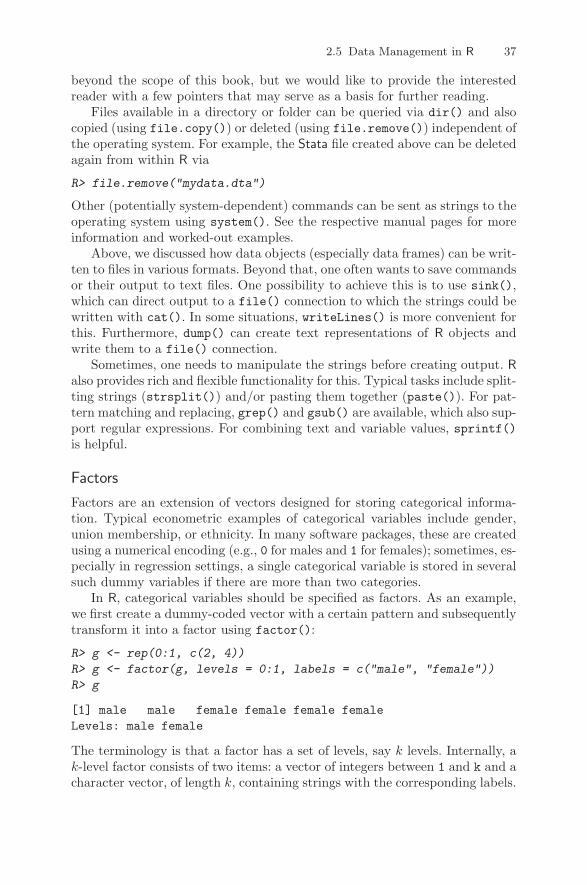
2.5 Data Management in R 37

beyond the scope of this book, but we would like to provide the interestedreader with a few pointers that may serve as a basis for further reading.

Files available in a directory or folder can be queried via dir() and alsocopied (using file.copy()) or deleted (using file.remove()) independent ofthe operating system. For example, the Stata file created above can be deletedagain from within R via

R> file.remove("mydata.dta")

Other (potentially system-dependent) commands can be sent as strings to theoperating system using system(). See the respective manual pages for moreinformation and worked-out examples.

Above, we discussed how data objects (especially data frames) can be writ-ten to files in various formats. Beyond that, one often wants to save commandsor their output to text files. One possibility to achieve this is to use sink(),which can direct output to a file() connection to which the strings could bewritten with cat(). In some situations, writeLines() is more convenient forthis. Furthermore, dump() can create text representations of R objects andwrite them to a file() connection.

Sometimes, one needs to manipulate the strings before creating output. Ralso provides rich and flexible functionality for this. Typical tasks include split-ting strings (strsplit()) and/or pasting them together (paste()). For pat-tern matching and replacing, grep() and gsub() are available, which also sup-port regular expressions. For combining text and variable values, sprintf()is helpful.

Factors

Factors are an extension of vectors designed for storing categorical informa-tion. Typical econometric examples of categorical variables include gender,union membership, or ethnicity. In many software packages, these are createdusing a numerical encoding (e.g., 0 for males and 1 for females); sometimes, es-pecially in regression settings, a single categorical variable is stored in severalsuch dummy variables if there are more than two categories.

In R, categorical variables should be specified as factors. As an example,we first create a dummy-coded vector with a certain pattern and subsequentlytransform it into a factor using factor():

R> g <- rep(0:1, c(2, 4))

R> g <- factor(g, levels = 0:1, labels = c("male", "female"))

R> g

[1] male male female female female femaleLevels: male female

The terminology is that a factor has a set of levels, say k levels. Internally, ak-level factor consists of two items: a vector of integers between 1 and k and acharacter vector, of length k, containing strings with the corresponding labels.

38 2 Basics

Above, we created the factor from an integer vector; alternatively, it could havebeen constructed from other numerical, character, or logical vectors. Ordinalinformation may also be stored in a factor by setting the argument ordered= TRUE when calling factor().

The advantage of this approach is that R knows when a certain variable iscategorical and can choose appropriate methods automatically. For example,the labels can be used in printed output, different summary and plottingmethods can be chosen, and contrast codings (e.g., dummy variables) can becomputed in linear regressions. Note that for these actions the ordering of thelevels can be important.

Missing values

Many data sets contain observations for which certain variables are unavail-able. Econometric software needs ways to deal with this. In R, such missingvalues are coded as NA (for “not available”). All standard computations on NAbecome NA.

Special care is needed when reading data that use a different encoding. Forexample, when preparing the package AER, we encountered several data setsthat employed -999 for missing values. If a file mydata.txt contains missingvalues coded in this way, they may be converted to NA using the argumentna.strings when reading the file:

R> newdata <- read.table("mydata.txt", na.strings = "-999")

To query whether certain observations are NA or not, the function is.na() isprovided.

2.6 Object Orientation

Somewhat vaguely, object-oriented programming (OOP) refers to a paradigmof programming where users/developers can create objects of a certain “class”(that are required to have a certain structure) and then apply “methods” forcertain “generic functions” to these objects. A simple example in R is thefunction summary(), which is a generic function choosing, depending on theclass of its argument, the summary method defined for this class. For example,for the numerical vector x and the factor g used above,

R> x <- c(1.8, 3.14, 4, 88.169, 13)

R> g <- factor(rep(c(0, 1), c(2, 4)), levels = c(0, 1),

+ labels = c("male", "female"))

the summary() call yields different types of results:

R> summary(x)

Min. 1st Qu. Median Mean 3rd Qu. Max.1.80 3.14 4.00 22.00 13.00 88.20

2.6 Object Orientation 39

R> summary(g)

male female2 4

For the numerical vector x, a five-number summary (i.e., the minimum andmaximum, the median, and the first and third quartiles) along with the meanare reported, and for the factor g a simple frequency table is returned. Thisshows that R has different summary() methods available for different types ofclasses (in particular, it knows that a five-number summary is not sensible forcategorical variables). In R, every object has a class that can be queried usingthe function class()

R> class(x)

[1] "numeric"

R> class(g)

[1] "factor"

which is used internally for calling the appropriate method for a generic func-tion.

In fact, R offers several paradigms of object orientation. The base installa-tion comes with two different OOP systems, usually called S3 (Chambers andHastie 1992) and S4 (Chambers 1998). The S3 system is much simpler, usinga dispatch mechanism based on a naming convention for methods. The S4 sys-tem is more sophisticated and closer to other OOP concepts used in computerscience, but it also requires more discipline and experience. For most tasks, S3is sufficient, and therefore it is the only OOP system (briefly) discussed here.

In S3, a generic function is defined as a function with a certain list ofarguments and then a UseMethod() call with the name of the generic function.For example, printing the function summary() reveals its definition:

R> summary

function (object, ...)UseMethod("summary")<environment: namespace:base>

It takes a first required argument object plus an arbitrary number of furtherarguments passed through ... to its methods. What happens if this functionis applied to an object, say of class “foo”, is that R tries to apply the functionsummary.foo() if it exists. If not, it will call summary.default() if sucha default method exists (which is the case for summary()). Furthermore, Robjects can have a vector of classes (e.g., c("foo", "bar"), which meansthat such objects are of class “foo” inheriting from “bar”). In this case, R firsttries to apply summary.foo(), then (if this does not exist) summary.bar(),and then (if both do not exist) summary.default(). All methods that are

40 2 Basics

currently defined for a generic function can be queried using methods(); e.g.,methods(summary) will return a (long) list of methods for all sorts of differentclasses. Among them is a method summary.factor(), which is used whensummary(g) is called. However, there is no summary.numeric(), and hencesummary(x) is handled by summary.default(). As it is not recommended tocall methods directly, some methods are marked as being non-visible to theuser, and these cannot (easily) be called directly. However, even for visiblemethods, we stress that in most situations it is clearly preferred to use, forexample, summary(g) instead of summary.factor(g).

To illustrate how easy it is to define a class and some methods for it, letus consider a simple example. We create an object of class “normsample” thatcontains a sample from a normal distribution and then define a summary()method that reports the empirical mean and standard deviation for this sam-ple. First, we write a simple class creator. In principle, it could have any name,but it is often called like the class itself:

R> normsample <- function(n, ...)

+ rval <- rnorm(n, ...)

+ class(rval) <- "normsample"

+ return(rval)

+

This function takes a required argument n (the sample size) and further argu-ments ..., which are passed on to rnorm(), the function for generating normalrandom numbers. In addition to the sample size, it takes further arguments—the mean and the standard deviation; see ?rnorm. After generation of thevector of normal random numbers, it is assigned the class “normsample” andthen returned.

R> set.seed(123)

R> x <- normsample(10, mean = 5)

R> class(x)

[1] "normsample"

To define a summary() method, we create a function summary.normsample()that conforms with the argument list of the generic (although ... is not usedhere) and computes the sample size, the empirical mean, and the standarddeviation.

R> summary.normsample <- function(object, ...)

+ rval <- c(length(object), mean(object), sd(object))

+ names(rval) <- c("sample size","mean","standard deviation")

+ return(rval)

+

Hence, calling

R> summary(x)

2.7 R Graphics 41

sample size mean standard deviation10.0000 5.0746 0.9538

automatically finds our new summary() method and yields the desired output.Other generic functions with methods for most standard R classes are

print(), plot(), and str(), which print, plot, and summarize the structureof an object, respectively.

2.7 R Graphics

It is no coincidence that early publications on S and R, such as Becker andChambers (1984) and Ihaka and Gentleman (1996), are entitled “S: An Inter-active Environment for Data Analysis and Graphics” and “R: A Language forData Analysis and Graphics”, respectively. R indeed has powerful graphics.

Here, we briefly introduce the “conventional” graphics as implemented inbase R. R also comes with a new and even more flexible graphics engine, calledgrid (see Murrell 2005), that provides the basis for an R implementation of“trellis”-type graphics (Cleveland 1993) in the package lattice (Sarkar 2002),but these are beyond the scope of this book. An excellent overview of Rgraphics is given in Murrell (2005).

The function plot()

The basic function is the default plot() method. It is a generic functionand has methods for many objects, including data frames, time series, andfitted linear models. Below, we describe the default plot() method, whichcan create various types of scatterplots, but many of the explanations extendto other methods as well as to other high-level plotting functions.

The scatterplot is probably the most common graphical display in statis-tics. A scatterplot of y vs. x is available using plot(x, y). For illustration,we again use the Journals data from our package AER, taken from Stock andWatson (2007). As noted in Section 1.1, the data provide some informationon subscriptions to economics journals at US libraries for the year 2000. Thefile contains 180 observations (the journals) on 10 variables, among them thenumber of library subscriptions (subs), the library subscription price (price),and the total number of citations for the journal (citations). These data willreappear in Chapter 3.

Here, we are interested in the relationship between the number of subscrip-tions and the price per citation. The following code chunk derives the requiredvariable citeprice and plots the number of library subscriptions against itin logarithms:

R> data("Journals")

R> Journals$citeprice <- Journals$price/Journals$citations

R> attach(Journals)

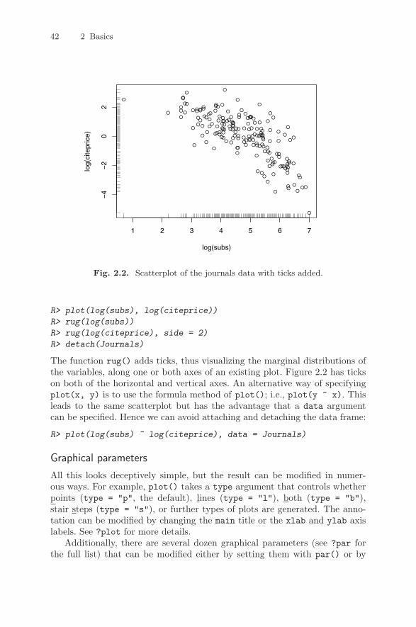
42 2 Basics

Fig. 2.2. Scatterplot of the journals data with ticks added.

R> plot(log(subs), log(citeprice))

R> rug(log(subs))

R> rug(log(citeprice), side = 2)

R> detach(Journals)

The function rug() adds ticks, thus visualizing the marginal distributions ofthe variables, along one or both axes of an existing plot. Figure 2.2 has tickson both of the horizontal and vertical axes. An alternative way of specifyingplot(x, y) is to use the formula method of plot(); i.e., plot(y ~ x). Thisleads to the same scatterplot but has the advantage that a data argumentcan be specified. Hence we can avoid attaching and detaching the data frame:

R> plot(log(subs) ~ log(citeprice), data = Journals)

Graphical parameters

All this looks deceptively simple, but the result can be modified in numer-ous ways. For example, plot() takes a type argument that controls whetherpoints (type = "p", the default), lines (type = "l"), both (type = "b"),stair steps (type = "s"), or further types of plots are generated. The anno-tation can be modified by changing the main title or the xlab and ylab axislabels. See ?plot for more details.

Additionally, there are several dozen graphical parameters (see ?par forthe full list) that can be modified either by setting them with par() or by

1 2 3 4 5 6 7

−4

−2

02

log(subs)

log(

cite

pric

e)

2.7 R Graphics 43

Table 2.1. A selective list of arguments to par().

Argument Description

axes should axes be drawn?bg background colorcex size of a point or symbolcol colorlas orientation of axis labelslty, lwd line type and line widthmain, sub title and subtitlemar size of marginsmfcol, mfrow array defining layout for several graphs on a plotpch plotting symboltype types (see text)xlab, ylab axis labelsxlim, ylim axis rangesxlog, ylog, log logarithmic scales

supplying them to the plot() function. We cannot explain all of these here,but we will highlight a few important parameters: col sets the color(s) andxlim and ylim adjust the plotting ranges. If points are plotted, pch can modifythe plotting character and cex its character extension. If lines are plotted, ltyand lwd specify the line type and width, respectively. The size of labels, axisticks, etc., can be changed by further cex-type arguments such as cex.laband cex.axis. A brief list of arguments to par() is provided in Table 2.1.This is just the tip of the iceberg, and further graphical parameters will beintroduced as we proceed.

As a simple example, readers may want to try

R> plot(log(subs) ~ log(citeprice), data = Journals, pch = 20,

+ col = "blue", ylim = c(0, 8), xlim = c(-7, 4),

+ main = "Library subscriptions")

This yields solid circles (pch = 20) instead of the default open ones, drawnin blue, and there are wider ranges in the x and y directions; there is also amain title.

It is also possible to add further layers to a plot. Thus, lines(), points(),text(), and legend() add what their names suggest to an existing plot. Forexample, text(-3.798, 5.846, "Econometrica", pos = 2) puts a charac-ter string at the indicated location (i.e., to the left of the point). In regressionanalyses, one often wants to add a regression line to a scatterplot. As seen inChapter 1, this is achieved using abline(a, b), where a is the intercept andb is the slope.

At this point, there does not seem to be a great need for all this; however,most users require fine control of visual displays at some point, especially whenpublication-quality plots are needed. We refrain from presenting artificial

44 2 Basics

examples toying with graphics options; instead we shall introduce variationsof the standard displays as we proceed.

Of course, there are many further plotting functions besides the defaultplot() method. For example, standard statistical displays such as barplots,pie charts, boxplots, QQ plots, or histograms are available in the functionsbarplot(), pie(), boxplot(), qqplot(), and hist(). It is instructive to rundemo("graphics") to obtain an overview of R’s impressive graphics facilities.

Exporting graphics

In interactive use, graphics are typically written to a graphics window sothat they can be inspected directly. However, after completing an analysis, wetypically want to save the resulting graphics (e.g., for publication in a report,journal article, or thesis). For users of Microsoft Windows and Microsoft Word,a simple option is to“copy and paste”them into the Microsoft Word document.For other programs, such as LATEX, it is preferable to export the graphic intoan external file. For this, there exist various graphics devices to which plotscan be written. Devices that are available on all platforms include the vectorformats PostScript and PDF; other devices, such as the bitmap formats PNGand JPEG and the vector format WMF, are only available if supported bythe system (see ?Devices for further details). They all work in the same way:first the device is opened—e.g., the PDF device is opened by the functionpdf()—then the commands creating the plot are executed, and finally thedevice is closed by dev.off(). A simple example creating a plot on a PDFdevice is:

R> pdf("myfile.pdf", height = 5, width = 6)

R> plot(1:20, pch = 1:20, col = 1:20, cex = 2)

R> dev.off()

This creates the PDF file myfile.pdf in the current working directory,which contains the graphic generated by the plot() call (see Figure 2.3).Incidentally, the plot illustrates a few of the parameters discussed above: itshows the first 20 plotting symbols (all shown in double size) and that in R aset of colors is also numbered. The first eight colors are black, red, green, blue,turquoise, violet, yellow, and gray. From color nine on, this vector is simplyrecycled.

Alternatively to opening, printing and closing a device, it is also possibleto print an existing plot in the graphics window to a device using dev.copy()and dev.print(); see the corresponding manual page for more information.

Mathematical annotation of plots

A feature that particularly adds to R’s strengths when it comes to publication-quality graphics is its ability to add mathematical annotation to plots (Murrelland Ihaka 2000). An S expression containing a mathematical expression can

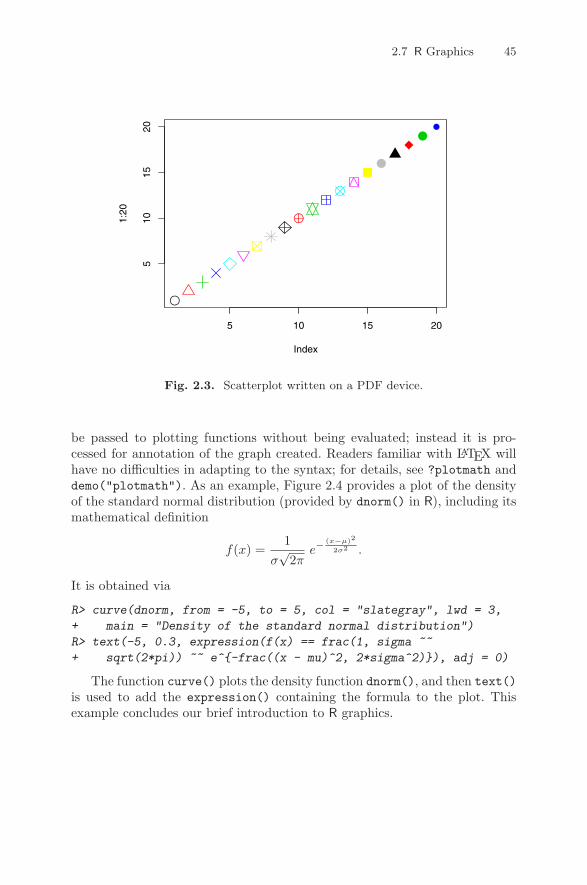
2.7 R Graphics 45

Fig. 2.3. Scatterplot written on a PDF device.

be passed to plotting functions without being evaluated; instead it is pro-cessed for annotation of the graph created. Readers familiar with LATEX willhave no difficulties in adapting to the syntax; for details, see ?plotmath anddemo("plotmath"). As an example, Figure 2.4 provides a plot of the densityof the standard normal distribution (provided by dnorm() in R), including itsmathematical definition

f(x) =1

σ√

2πe−

(x−µ)2

2σ2 .

It is obtained via

R> curve(dnorm, from = -5, to = 5, col = "slategray", lwd = 3,

+ main = "Density of the standard normal distribution")

R> text(-5, 0.3, expression(f(x) == frac(1, sigma ~~

+ sqrt(2*pi)) ~~ e^-frac((x - mu)^2, 2*sigma^2)), adj = 0)

The function curve() plots the density function dnorm(), and then text()is used to add the expression() containing the formula to the plot. Thisexample concludes our brief introduction to R graphics.

5 10 15 20

510

1520

Index

1:20

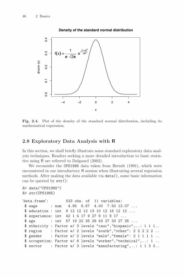
46 2 Basics

Fig. 2.4. Plot of the density of the standard normal distribution, including itsmathematical expression.

2.8 Exploratory Data Analysis with R

In this section, we shall briefly illustrate some standard exploratory data anal-ysis techniques. Readers seeking a more detailed introduction to basic statis-tics using R are referred to Dalgaard (2002).

We reconsider the CPS1985 data taken from Berndt (1991), which wereencountered in our introductory R session when illustrating several regressionmethods. After making the data available via data(), some basic informationcan be queried by str():

R> data("CPS1985")

R> str(CPS1985)

'data.frame': 533 obs. of 11 variables:$ wage : num 4.95 6.67 4.00 7.50 13.07 ...$ education : int 9 12 12 12 13 10 12 16 12 12 ...$ experience: int 42 1 4 17 9 27 9 11 9 17 ...$ age : int 57 19 22 35 28 43 27 33 27 35 ...$ ethnicity : Factor w/ 3 levels "cauc","hispanic",..: 1 1 1..$ region : Factor w/ 2 levels "south","other": 2 2 2 2 2 ..$ gender : Factor w/ 2 levels "male","female": 2 1 1 1 1 ..$ occupation: Factor w/ 6 levels "worker","technical",..: 1 ..$ sector : Factor w/ 3 levels "manufacturing",..: 1 1 3 3..

−4 −2 0 2 4

0.0

0.1

0.2

0.3

0.4

Density of the standard normal distribution

x

dnor

m (

x)

f((x)) ==1

σσ 2ππ e−−((x−−μμ))2

2σσ2

2.8 Exploratory Data Analysis with R 47

$ union : Factor w/ 2 levels "no","yes": 1 1 1 1 2 1 1 1..$ married : Factor w/ 2 levels "no","yes": 2 1 1 2 1 1 1 2..

This reveals that this “data.frame” object comprises 533 observations on11 variables, including the numerical variable wage, the integer variableseducation, experience, and age, and seven factors, each comprising twoto six levels.

Instead of using the list-type view that str() provides, it is often usefulto inspect the top (or the bottom) of a data frame in its rectangular repre-sentation. For this purpose, there exist the convenience functions head() andtail(), returning (by default) the first and last six rows, respectively. Thus

R> head(CPS1985)

wage education experience age ethnicity region gender1 4.95 9 42 57 cauc other female2 6.67 12 1 19 cauc other male3 4.00 12 4 22 cauc other male4 7.50 12 17 35 cauc other male5 13.07 13 9 28 cauc other male6 4.45 10 27 43 cauc south maleoccupation sector union married

1 worker manufacturing no yes2 worker manufacturing no no3 worker other no no4 worker other no yes5 worker other yes no6 worker other no no

Another useful way of gaining a quick overview of a data set is to use thesummary() method for data frames, which provides a summary for each of thevariables. As the type of the summary depends on the class of the respectivevariable, we inspect the summary() methods separately for various variablesfrom CPS1985 below. Hence, the output of summary(CPS1985) is omitted here.

As the CPS1985 data are employed repeatedly in the following, we avoidlengthy commands such as CPS1985$education by attaching the data set.Also, to compactify subsequent output, we abbreviate two levels of occupationfrom "technical" to "techn" and from "management" to "mgmt".

R> levels(CPS1985$occupation)[c(2, 6)] <- c("techn", "mgmt")

R> attach(CPS1985)

Now variables are accessible by their names.We proceed by illustrating exploratory analysis of single as well as pairs of

variables, distinguishing among numerical variables, factors, and combinationsthereof. We begin with the simplest kind, a single numerical variable.

48 2 Basics

One numerical variable

We will first look at the distribution of wages in the sample:

R> summary(wage)

Min. 1st Qu. Median Mean 3rd Qu. Max.1.00 5.25 7.78 9.03 11.20 44.50

This provides Tukey’s five-number summary plus the mean wage. The meanand median could also have been obtained using

R> mean(wage)

[1] 9.031

R> median(wage)

[1] 7.78

and fivenum() computes the five-number summary. Similarly, min() andmax() would have yielded the minimum and the maximum. Arbitrary quan-tiles can be computed by quantile().

For measures of spread, there exist the functions

R> var(wage)

[1] 26.43

R> sd(wage)

[1] 5.141

returning the variance and the standard deviation, respectively.Graphical summaries are also helpful. For numerical variables such as wage,

density visualizations (via histograms or kernel smoothing) and boxplots aresuitable. Boxplots will be considered below in connection with two-variabledisplays. Figure 2.5, obtained via

R> hist(wage, freq = FALSE)

R> hist(log(wage), freq = FALSE)

R> lines(density(log(wage)), col = 4)

shows the densities of wage and its logarithm (that is, areas under curvesequal 1, resulting from freq = FALSE; otherwise absolute frequencies wouldhave been depicted). Further arguments allow for fine tuning of the selectionof the breaks in the histogram. Added to the histogram in the right panel is akernel density estimate obtained using density(). Clearly, the distribution ofthe logarithms is less skewed than that of the raw data. Note that density()only computes the density coordinates and does not provide a plot; hence theestimate is added via lines().

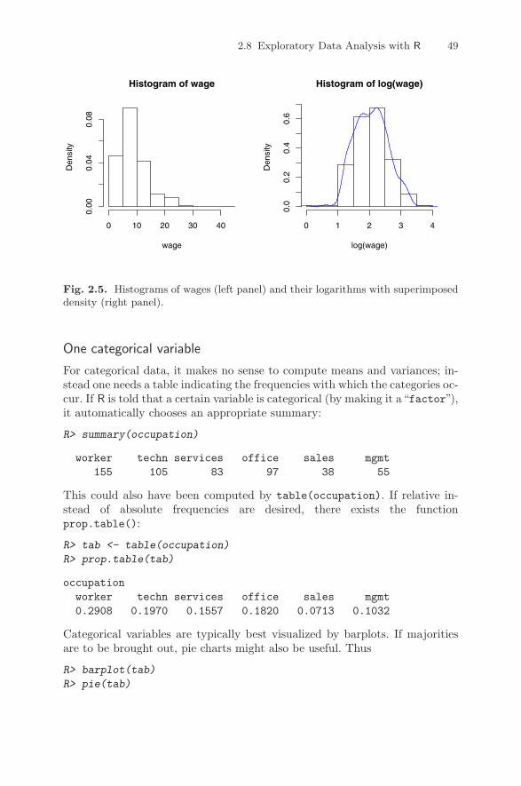
2.8 Exploratory Data Analysis with R 49

Fig. 2.5. Histograms of wages (left panel) and their logarithms with superimposeddensity (right panel).

One categorical variable

For categorical data, it makes no sense to compute means and variances; in-stead one needs a table indicating the frequencies with which the categories oc-cur. If R is told that a certain variable is categorical (by making it a“factor”),it automatically chooses an appropriate summary:

R> summary(occupation)

worker techn services office sales mgmt155 105 83 97 38 55

This could also have been computed by table(occupation). If relative in-stead of absolute frequencies are desired, there exists the functionprop.table():

R> tab <- table(occupation)

R> prop.table(tab)

occupationworker techn services office sales mgmt0.2908 0.1970 0.1557 0.1820 0.0713 0.1032

Categorical variables are typically best visualized by barplots. If majoritiesare to be brought out, pie charts might also be useful. Thus

R> barplot(tab)

R> pie(tab)

Histogram of wage

wage

Den

sity

0 10 20 30 40

0.00

0.04

0.08

Histogram of log(wage)

log(wage)

Den

sity

0 1 2 3 4

0.0

0.2

0.4

0.6

50 2 Basics

Fig. 2.6. Bar plot and pie chart of occupation.

provides Figure 2.6. Note that both functions expect the tabulated fre-quencies as input. In addition, calling plot(occupation) is equivalent tobarplot(table(occupation)).

Two categorical variables

The relationship between two categorical variables is typically summarized bya contingency table. This can be created either by xtabs(), a function witha formula interface, or by table(), a function taking an arbitrary number ofvariables for cross-tabulation (and not only a single one as shown above).

We consider the factors occupation and gender for illustration:

R> xtabs(~ gender + occupation, data = CPS1985)

occupationgender worker techn services office sales mgmtmale 126 53 34 21 21 34female 29 52 49 76 17 21

which can equivalently be created by table(gender, occupation). A simplevisualization is a mosaic plot (Hartigan and Kleiner 1981; Friendly 1994),which can be seen as a generalization of stacked barplots. The plot given inFigure 2.7 (also known as a “spine plot”, a certain variant of the standardmosaic display), obtained via

R> plot(gender ~ occupation, data = CPS1985)

shows that the proportion of males and females changes considerablyover the levels of occupation. In addition to the shading that brings out the

wor

ker

tech

n

serv

ices

offic

e

sale

s

mgm

t

050

100

150

workertechn

services

office

sales

mgmt

2.8 Exploratory Data Analysis with R 51

Fig. 2.7. Mosaic plot (spine plot) of gender versus occupation.

conditional distribution of gender given occupation, the widths of the barsvisualize the marginal distribution of occupation, indicating that there arecomparatively many workers and few salespersons.

Two numerical variables

We exemplify the exploratory analysis of the relationship between two numer-ical variables by using wage and education.

A summary measure for two numerical variables is the correlation coeffi-cient, implemented in the function cor(). However, the standard (Pearson)correlation coefficient is not necessarily meaningful for positive and heavilyskewed variables such as wage. We therefore also compute a nonparametricvariant, Spearman’s %, which is available in cor() as an option.

R> cor(log(wage), education)

[1] 0.379

R> cor(log(wage), education, method = "spearman")

[1] 0.3798

Both measures are virtually identical and indicate only a modest amount ofcorrelation here, see also the corresponding scatterplot in Figure 2.8:

R> plot(log(wage) ~ education)

occupation

gend

er

worker techn services office sales mgmt

mal

efe

mal

e

0.0

0.2

0.4

0.6

0.8

1.0

52 2 Basics

Fig. 2.8. Scatterplot of wages (in logs) versus education.

One numerical and one categorical variable

It is common to have both numerical and categorical variables in a data frame.For example, here we have wage and gender, and there might be some interestin the distribution of wage by gender. A suitable function for numerical sum-maries is tapply(). It applies, for a numerical variable as its first argumentand a (list of) categorical variable(s) as its second argument, the functionspecified as the third argument. Hence, mean wages conditional on gender areavailable using

R> tapply(log(wage), gender, mean)

male female2.165 1.935

Using similar commands, further descriptive measures or even entire sum-maries (just replace mean by summary) may be computed.

Suitable graphical displays are parallel boxplots and quantile-quantile(QQ) plots, as depicted in Figure 2.9. Recall that a boxplot (or “box-and-whiskers plot”) is a coarse graphical summary of an empirical distribution.The box indicates “hinges” (approximately the lower and upper quartiles) andthe median. The “whiskers” (lines) indicate the largest and smallest observa-tions falling within a distance of 1.5 times the box size from the nearest hinge.Any observations falling outside this range are shown separately and would

5 10 15

01

23

education

log(

wag

e)

2.8 Exploratory Data Analysis with R 53

Fig. 2.9. Boxplot and QQ plot of wages stratified by gender.

be considered extreme or outlying (in an approximately normal sample). Notethat there are several variants of boxplots in the literature.

The commands plot(y ~ x) and boxplot(y ~ x) both yield the sameparallel boxplot if x is a “factor”; thus

R> plot(log(wage) ~ gender)

gives the left panel of Figure 2.9. It shows that the overall shapes of bothdistributions are quite similar and that males enjoy a substantial advantage,especially in the medium range. The latter feature is also brought out by theQQ plot (right panel) resulting from

R> mwage <- subset(CPS1985, gender == "male")$wage

R> fwage <- subset(CPS1985, gender == "female")$wage

R> qqplot(mwage, fwage, xlim = range(wage), ylim = range(wage),

+ xaxs = "i", yaxs = "i", xlab = "male", ylab = "female")

R> abline(0, 1)

where almost all points are below the diagonal (corresponding to identicaldistributions in both samples). This indicates that, for most quantiles, malewages are typically higher than female wages.

We end this section by detaching the data:

R> detach(CPS1985)

male female

01

23

gender

log(

wag

e)

10 20 30 40

1020

3040

male

fem

ale

54 2 Basics

2.9 Exercises

1. Create a square matrix, say A, with entries aii = 2, i = 2, . . . , n − 1,a11 = ann = 1, ai,i+1 = ai,i−1 = −1, and aij = 0 elsewhere. (Where doesthis matrix occur in econometrics?)

2. “PARADE”is the Sunday newspaper magazine supplementing the Sundayor weekend edition of some 500 daily newspapers in the United States ofAmerica. An important yearly feature is an article providing informationon some 120–150 “randomly” selected US citizens, indicating their pro-fession, hometown and state, and their yearly earnings. The Parade2005data contain the 2005 version, amended by a variable indicating celebritystatus (motivated by substantial oversampling of celebrities in these data).For the Parade2005 data:(a) Determine the mean earnings in California. Explain the result.(b) Determine the number of individuals residing in Idaho. (What does

this say about the data set?)(c) Determine the mean and the median earnings of celebrities. Comment.(d) Obtain boxplots of log(earnings) stratified by celebrity. Com-

ment.3. For the Parade2005 data of the preceding exercise, obtain a kernel den-

sity estimate of the earnings for the full data set. It will be necessaryto transform the data to logarithms (why?). Comment on the result. Besure to try out some arguments to density(), in particular the plug-inbandwidth bw.

4. Consider the CPS1988 data, taken from Bierens and Ginther (2001).(These data will be used for estimating an earnings equation in the nextchapter.)(a) Obtain scatterplots of the logarithm of the real wage (wage) versus

experience and versus education.(b) In fact, education corresponds to years of schooling and therefore

takes on only a limited number of values. Transform education intoa factor and obtain parallel boxplots of wage stratified by the levelsof education. Repeat for experience.

(c) The data set contains four additional factors, ethnicity, smsa,region, and parttime. Obtain suitable graphical displays of log(wage)versus each of these factors.

3

Linear Regression

The linear regression model, typically estimated by ordinary least squares(OLS), is the workhorse of applied econometrics. The model is

yi = x>i β + εi, i = 1, . . . , n,

or, in matrix form,y = Xβ + ε,

where y is an n×1 vector containing the dependent variable, xi is the (column)vector of covariates for observation i—thus X = (x1, . . . , xn)> is the n×k re-gressor matrix, or model matrix (whose columns contain the regressors)—andβ is a k×1 vector of regression coefficients. Furthermore, ε is the n×1 vectorof disturbances (or error terms). Assumptions on the error terms depend onthe context. For cross sections, E(ε|X) = 0 (exogeneity) and Var(ε|X) = σ2I(conditional homoskedasticity and lack of correlation) are common. However,for time series data, exogeneity is too strong an assumption, and it is com-monly replaced by predeterminedness; i.e., E(εj |xi) = 0, i ≤ j. Methods forchecking these assumptions are discussed in Chapter 4.

We assume that readers are familiar with the basics of the linear regressionmodel, say at the level of Baltagi (2002) or Greene (2003). To fix notation, letβ = (X>X)−1X>y denote the familiar OLS estimator of β. The correspond-ing fitted values are y = Xβ, the residuals are ε = y− y, and the residual sumof squares (RSS) is ε>ε.

In R, models are typically fitted by calling a model-fitting function, in thiscase lm(), with a “formula” object describing the model and a “data.frame”object containing the variables used in the formula. Most fitting functions,including lm(), take further arguments, providing a more detailed descriptionof the model or control parameters for the fitting algorithm. By subsumingsuch further arguments in ..., a prototypical call looks like

fm <- lm(formula, data, ...)

C. Kleiber, A. Zeileis, Applied Econometrics with R,DOI: 10.1007/978-0-387-77318-6 3, © Springer Science+Business Media, LLC 2008

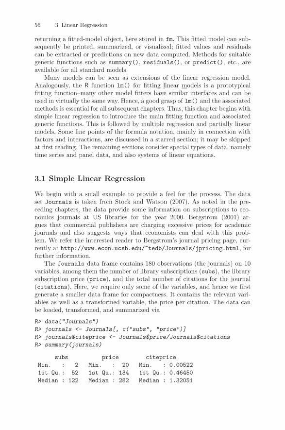
56 3 Linear Regression

returning a fitted-model object, here stored in fm. This fitted model can sub-sequently be printed, summarized, or visualized; fitted values and residualscan be extracted or predictions on new data computed. Methods for suitablegeneric functions such as summary(), residuals(), or predict(), etc., areavailable for all standard models.

Many models can be seen as extensions of the linear regression model.Analogously, the R function lm() for fitting linear models is a prototypicalfitting function–many other model fitters have similar interfaces and can beused in virtually the same way. Hence, a good grasp of lm() and the associatedmethods is essential for all subsequent chapters. Thus, this chapter begins withsimple linear regression to introduce the main fitting function and associatedgeneric functions. This is followed by multiple regression and partially linearmodels. Some fine points of the formula notation, mainly in connection withfactors and interactions, are discussed in a starred section; it may be skippedat first reading. The remaining sections consider special types of data, namelytime series and panel data, and also systems of linear equations.

3.1 Simple Linear Regression

We begin with a small example to provide a feel for the process. The dataset Journals is taken from Stock and Watson (2007). As noted in the pre-ceding chapters, the data provide some information on subscriptions to eco-nomics journals at US libraries for the year 2000. Bergstrom (2001) ar-gues that commercial publishers are charging excessive prices for academicjournals and also suggests ways that economists can deal with this prob-lem. We refer the interested reader to Bergstrom’s journal pricing page, cur-rently at http://www.econ.ucsb.edu/~tedb/Journals/jpricing.html, forfurther information.

The Journals data frame contains 180 observations (the journals) on 10variables, among them the number of library subscriptions (subs), the librarysubscription price (price), and the total number of citations for the journal(citations). Here, we require only some of the variables, and hence we firstgenerate a smaller data frame for compactness. It contains the relevant vari-ables as well as a transformed variable, the price per citation. The data canbe loaded, transformed, and summarized via

R> data("Journals")

R> journals <- Journals[, c("subs", "price")]

R> journals$citeprice <- Journals$price/Journals$citations

R> summary(journals)

subs price citepriceMin. : 2 Min. : 20 Min. : 0.005221st Qu.: 52 1st Qu.: 134 1st Qu.: 0.46450Median : 122 Median : 282 Median : 1.32051

3.1 Simple Linear Regression 57

Fig. 3.1. Scatterplot of the journals data with least-squares line.

Mean : 197 Mean : 418 Mean : 2.548453rd Qu.: 268 3rd Qu.: 541 3rd Qu.: 3.44017Max. :1098 Max. :2120 Max. :24.45946

In view of the wide range of the variables, combined with a considerableamount of skewness, it is useful to take logarithms.

The goal is to estimate the effect of the price per citation on the number oflibrary subscriptions. To explore this issue quantitatively, we will fit a linearregression model,

log(subs)i = β1 + β2 log(citeprice)i + εi.

The primary function for this is lm(), which estimates a linear regression usingordinary least squares (OLS). As motivated above, a linear model is fitted bysupplying a formula that describes the model plus a data frame.

Here, the formula of interest is log(subs) ~ log(citeprice); i.e.,log(subs) explained by log(citeprice). This can be used both for plot-ting and for model fitting:

R> plot(log(subs) ~ log(citeprice), data = journals)

R> jour_lm <- lm(log(subs) ~ log(citeprice), data = journals)

R> abline(jour_lm)

The resulting plot is shown in Figure 3.1. abline() extracts the coefficientsof the fitted model and adds the corresponding regression line to the plot.

−4 −2 0 2

12

34

56

7

log(citeprice)

log(

subs

)

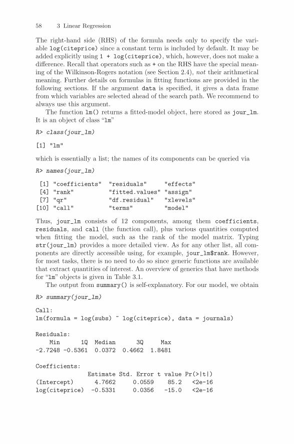
58 3 Linear Regression

The right-hand side (RHS) of the formula needs only to specify the vari-able log(citeprice) since a constant term is included by default. It may beadded explicitly using 1 + log(citeprice), which, however, does not make adifference. Recall that operators such as + on the RHS have the special mean-ing of the Wilkinson-Rogers notation (see Section 2.4), not their arithmeticalmeaning. Further details on formulas in fitting functions are provided in thefollowing sections. If the argument data is specified, it gives a data framefrom which variables are selected ahead of the search path. We recommend toalways use this argument.

The function lm() returns a fitted-model object, here stored as jour_lm.It is an object of class “lm”

R> class(jour_lm)

[1] "lm"

which is essentially a list; the names of its components can be queried via

R> names(jour_lm)

[1] "coefficients" "residuals" "effects"[4] "rank" "fitted.values" "assign"[7] "qr" "df.residual" "xlevels"[10] "call" "terms" "model"

Thus, jour_lm consists of 12 components, among them coefficients,residuals, and call (the function call), plus various quantities computedwhen fitting the model, such as the rank of the model matrix. Typingstr(jour_lm) provides a more detailed view. As for any other list, all com-ponents are directly accessible using, for example, jour_lm$rank. However,for most tasks, there is no need to do so since generic functions are availablethat extract quantities of interest. An overview of generics that have methodsfor “lm” objects is given in Table 3.1.

The output from summary() is self-explanatory. For our model, we obtain

R> summary(jour_lm)

Call:lm(formula = log(subs) ~ log(citeprice), data = journals)

Residuals:Min 1Q Median 3Q Max

-2.7248 -0.5361 0.0372 0.4662 1.8481

Coefficients:Estimate Std. Error t value Pr(>|t|)

(Intercept) 4.7662 0.0559 85.2 <2e-16log(citeprice) -0.5331 0.0356 -15.0 <2e-16

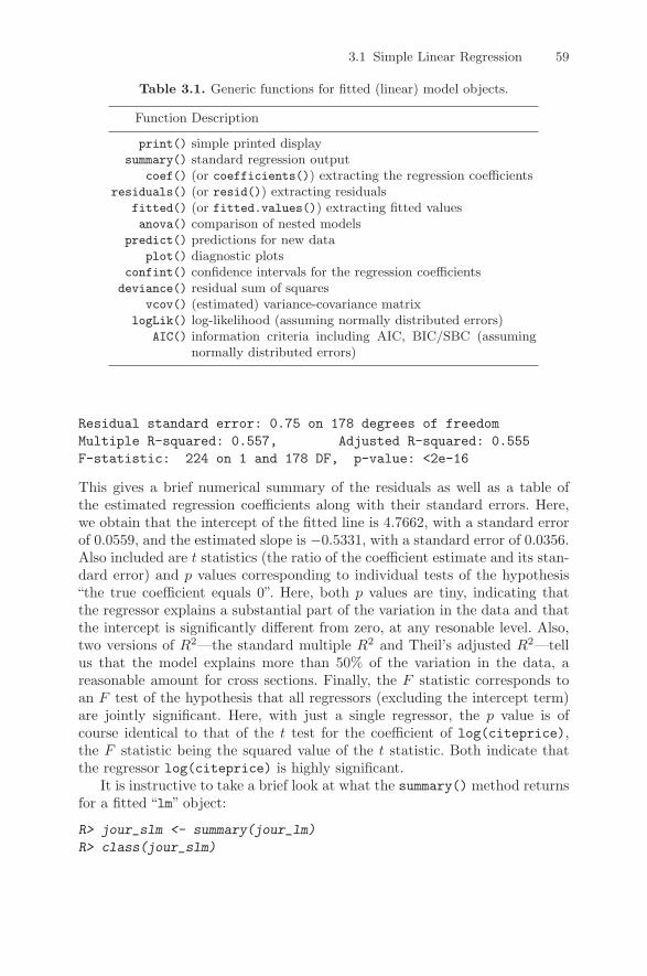
3.1 Simple Linear Regression 59

Table 3.1. Generic functions for fitted (linear) model objects.

Function Description

print() simple printed displaysummary() standard regression output

coef() (or coefficients()) extracting the regression coefficientsresiduals() (or resid()) extracting residuals

fitted() (or fitted.values()) extracting fitted valuesanova() comparison of nested models

predict() predictions for new dataplot() diagnostic plots

confint() confidence intervals for the regression coefficientsdeviance() residual sum of squares

vcov() (estimated) variance-covariance matrixlogLik() log-likelihood (assuming normally distributed errors)

AIC() information criteria including AIC, BIC/SBC (assumingnormally distributed errors)

Residual standard error: 0.75 on 178 degrees of freedomMultiple R-squared: 0.557, Adjusted R-squared: 0.555F-statistic: 224 on 1 and 178 DF, p-value: <2e-16

This gives a brief numerical summary of the residuals as well as a table ofthe estimated regression coefficients along with their standard errors. Here,we obtain that the intercept of the fitted line is 4.7662, with a standard errorof 0.0559, and the estimated slope is −0.5331, with a standard error of 0.0356.Also included are t statistics (the ratio of the coefficient estimate and its stan-dard error) and p values corresponding to individual tests of the hypothesis“the true coefficient equals 0”. Here, both p values are tiny, indicating thatthe regressor explains a substantial part of the variation in the data and thatthe intercept is significantly different from zero, at any resonable level. Also,two versions of R2—the standard multiple R2 and Theil’s adjusted R2—tellus that the model explains more than 50% of the variation in the data, areasonable amount for cross sections. Finally, the F statistic corresponds toan F test of the hypothesis that all regressors (excluding the intercept term)are jointly significant. Here, with just a single regressor, the p value is ofcourse identical to that of the t test for the coefficient of log(citeprice),the F statistic being the squared value of the t statistic. Both indicate thatthe regressor log(citeprice) is highly significant.

It is instructive to take a brief look at what the summary() method returnsfor a fitted “lm” object:

R> jour_slm <- summary(jour_lm)

R> class(jour_slm)

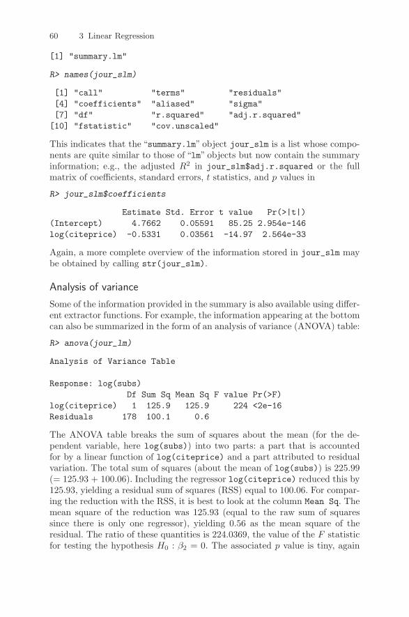
60 3 Linear Regression

[1] "summary.lm"

R> names(jour_slm)

[1] "call" "terms" "residuals"[4] "coefficients" "aliased" "sigma"[7] "df" "r.squared" "adj.r.squared"[10] "fstatistic" "cov.unscaled"

This indicates that the “summary.lm” object jour_slm is a list whose compo-nents are quite similar to those of “lm” objects but now contain the summaryinformation; e.g., the adjusted R2 in jour_slm$adj.r.squared or the fullmatrix of coefficients, standard errors, t statistics, and p values in

R> jour_slm$coefficients

Estimate Std. Error t value Pr(>|t|)(Intercept) 4.7662 0.05591 85.25 2.954e-146log(citeprice) -0.5331 0.03561 -14.97 2.564e-33

Again, a more complete overview of the information stored in jour_slm maybe obtained by calling str(jour_slm).

Analysis of variance

Some of the information provided in the summary is also available using differ-ent extractor functions. For example, the information appearing at the bottomcan also be summarized in the form of an analysis of variance (ANOVA) table:

R> anova(jour_lm)

Analysis of Variance Table

Response: log(subs)Df Sum Sq Mean Sq F value Pr(>F)

log(citeprice) 1 125.9 125.9 224 <2e-16Residuals 178 100.1 0.6

The ANOVA table breaks the sum of squares about the mean (for the de-pendent variable, here log(subs)) into two parts: a part that is accountedfor by a linear function of log(citeprice) and a part attributed to residualvariation. The total sum of squares (about the mean of log(subs)) is 225.99(= 125.93 + 100.06). Including the regressor log(citeprice) reduced this by125.93, yielding a residual sum of squares (RSS) equal to 100.06. For compar-ing the reduction with the RSS, it is best to look at the column Mean Sq. Themean square of the reduction was 125.93 (equal to the raw sum of squaressince there is only one regressor), yielding 0.56 as the mean square of theresidual. The ratio of these quantities is 224.0369, the value of the F statisticfor testing the hypothesis H0 : β2 = 0. The associated p value is tiny, again

3.1 Simple Linear Regression 61

indicating that the regressor log(citeprice) is highly significant. Of course,this is exactly the F test given in the summary above, which in turn is equiva-lent to the t test, as noted before. The column Df provides degrees of freedom(df): 1 df is attributed to the regressor log(citeprice), while 180− 2 = 178are attributed to the residuals (two regression coefficients were estimated).

The anova() method not only can produce an ANOVA table for a single“lm” object, but can also be used to compare several nested “lm” models usingF tests. This will be illustrated in the next section.

Point and interval estimates

To extract the estimated regression coefficients β, the function coef() can beused:

R> coef(jour_lm)

(Intercept) log(citeprice)4.7662 -0.5331

It is good practice to give a measure of error along with every estimate. Oneway to do this is to provide a confidence interval. This is available via theextractor function confint(); thus

R> confint(jour_lm, level = 0.95)

2.5 % 97.5 %(Intercept) 4.6559 4.8765log(citeprice) -0.6033 -0.4628

The default level is 95%, so specification of level = 0.95 was not reallyneeded here.

Prediction

Often a regression model is used for prediction. Recall that there are twotypes of predictions: the prediction of points on the regression line and theprediction of a new data value. The standard errors of predictions for newdata take into account both the uncertainty in the regression line and thevariation of the individual points about the line. Thus, the prediction intervalfor prediction of new data is larger than that for prediction of points on theline. The function predict() provides both types of standard errors.

For the journals data, we might be interested in the expected number ofsubscriptions for a journal whose price per citation equals 2.11 (this roughlycorresponds to the value for the Journal of Applied Econometrics, a journalthat is owned by a commercial publisher and fairly expensive) or in the numberof library subscriptions itself. Both types of prediction intervals are given bythe following code:

62 3 Linear Regression

R> predict(jour_lm, newdata = data.frame(citeprice = 2.11),

+ interval = "confidence")

fit lwr upr1 4.368 4.247 4.489

R> predict(jour_lm, newdata = data.frame(citeprice = 2.11),

+ interval = "prediction")

fit lwr upr1 4.368 2.884 5.853

Of course, the point estimates (denoted fit) are identical; only the inter-vals differ. Recall that these intervals are based on the t distribution with178 df (residual df in our case) and are exact under the assumption of (condi-tionally) normally distributed disturbances. By default, no intervals are com-puted and the data used for fitting are also used as newdata, so that bothpredict(jour_lm) and fitted(jour_lm) compute the fitted values y.

The prediction intervals can also be used for computing and visualizingconfidence bands. In the following code chunk, we set up an auxiliary variablelciteprice with equidistant points on the scale of log(citeprice), thencompute the corresponding prediction intervals, and finally visualize themusing plot() and lines(), which here adds the lines for the fitted values andthe confidence bands. The resulting plot is shown in Figure 3.2.

R> lciteprice <- seq(from = -6, to = 4, by = 0.25)

R> jour_pred <- predict(jour_lm, interval = "prediction",

+ newdata = data.frame(citeprice = exp(lciteprice)))

R> plot(log(subs) ~ log(citeprice), data = journals)

R> lines(jour_pred[, 1] ~ lciteprice, col = 1)

R> lines(jour_pred[, 2] ~ lciteprice, col = 1, lty = 2)

R> lines(jour_pred[, 3] ~ lciteprice, col = 1, lty = 2)

Plotting“lm”objects

The plot() method for class lm() provides six types of diagnostic plots, fourof which are shown by default. Figure 3.3 depicts the result for the journalsregression. We set the graphical parameter mfrow to c(2, 2) using the par()function, creating a 2× 2 matrix of plotting areas to see all four plots simul-taneously:

R> par(mfrow = c(2, 2))

R> plot(jour_lm)

R> par(mfrow = c(1, 1))

The first provides a graph of residuals versus fitted values, perhaps the mostfamiliar of all diagnostic plots for residual analysis. The second is a QQ plotfor normality. Its curvature (or rather its lack thereof) shows that the residuals

3.1 Simple Linear Regression 63

Fig. 3.2. Scatterplot with prediction intervals for the journals data.

more or less conform with normality. Plots three and four are a scale-locationplot and a plot of standardized residuals against leverages, respectively. Theirdiscussion will be postponed to Chapter 4. For the moment, we just note thatplot(jour_lm) already provides some indication of the fit of the model.

In our case, there appear to be difficulties with observations “MEPiTE”,“RoRPE”, “IO”, “BoIES”, and“Ecnmt”, corresponding to the journals MOCT-MOST: Economic Policy in Transitional Economics, Review of Radical Polit-ical Economics, International Organization, Bulletin of Indonesian EconomicStudies, and Econometrica, each of which is singled out in at least one of thefour plots. A closer look reveals that all these journals are not overly expen-sive, they are unusual in that they are either heavily cited (Econometrica),resulting in a low price per citation, or have only a few citations, resulting ina rather high price per citation. Incidentally, all plots may be accessed indi-vidually using, for example, plot(jour_lm, which = 2), if only the QQ plotis desired.

Testing a linear hypothesis

The standard regression output as provided by summary() only indicates in-dividual significance of each regressor and joint significance of all regressors inthe form of t and F statistics, respectively. Often it is necessary to test moregeneral hypotheses. This is possible using the function linear.hypothesis()from the car package, the package accompanying Fox (2002). (car will

−4 −2 0 2

12

34

56

7

log(citeprice)

log(

subs

)

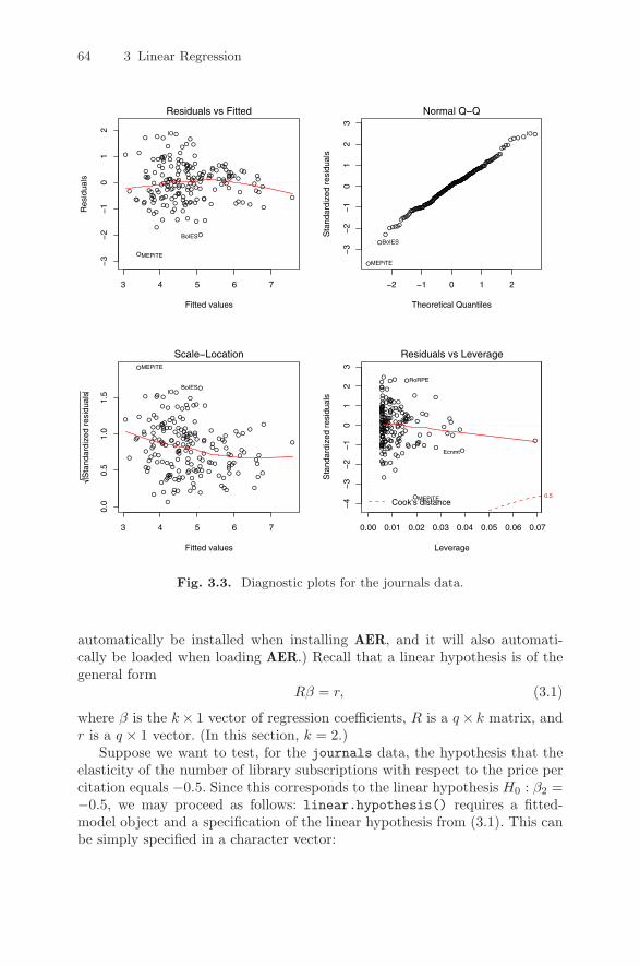
64 3 Linear Regression

Fig. 3.3. Diagnostic plots for the journals data.

automatically be installed when installing AER, and it will also automati-cally be loaded when loading AER.) Recall that a linear hypothesis is of thegeneral form

Rβ = r, (3.1)

where β is the k× 1 vector of regression coefficients, R is a q× k matrix, andr is a q × 1 vector. (In this section, k = 2.)

Suppose we want to test, for the journals data, the hypothesis that theelasticity of the number of library subscriptions with respect to the price percitation equals −0.5. Since this corresponds to the linear hypothesis H0 : β2 =−0.5, we may proceed as follows: linear.hypothesis() requires a fitted-model object and a specification of the linear hypothesis from (3.1). This canbe simply specified in a character vector:

3 4 5 6 7

−3

−2

−1

01

2

Fitted values

Res

idua

ls

Residuals vs Fitted

MEPiTE

BoIES

IO

−2 −1 0 1 2

−3

−2

−1

01

23

Theoretical Quantiles

Sta

ndar

dize

d re

sidu

als

Normal Q−Q

MEPiTE

BoIES

IO

3 4 5 6 7

0.0

0.5

1.0

1.5

Fitted values

Sta

ndar

dize

d re

sidu

als

Scale−LocationMEPiTE

BoIESIO

0.00 0.01 0.02 0.03 0.04 0.05 0.06 0.07

−4

−3

−2

−1

01

23

Leverage

Sta

ndar

dize

d re

sidu

als

Cook's distance0.5

Residuals vs Leverage

MEPiTE

RoRPE

Ecnmt

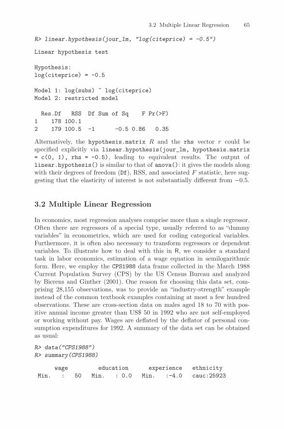
3.2 Multiple Linear Regression 65

R> linear.hypothesis(jour_lm, "log(citeprice) = -0.5")

Linear hypothesis test

Hypothesis:log(citeprice) = -0.5

Model 1: log(subs) ~ log(citeprice)Model 2: restricted model

Res.Df RSS Df Sum of Sq F Pr(>F)1 178 100.12 179 100.5 -1 -0.5 0.86 0.35

Alternatively, the hypothesis.matrix R and the rhs vector r could bespecified explicitly via linear.hypothesis(jour_lm, hypothesis.matrix= c(0, 1), rhs = -0.5), leading to equivalent results. The output oflinear.hypothesis() is similar to that of anova(): it gives the models alongwith their degrees of freedom (Df), RSS, and associated F statistic, here sug-gesting that the elasticity of interest is not substantially different from −0.5.

3.2 Multiple Linear Regression

In economics, most regression analyses comprise more than a single regressor.Often there are regressors of a special type, usually referred to as “dummyvariables” in econometrics, which are used for coding categorical variables.Furthermore, it is often also necessary to transform regressors or dependentvariables. To illustrate how to deal with this in R, we consider a standardtask in labor economics, estimation of a wage equation in semilogarithmicform. Here, we employ the CPS1988 data frame collected in the March 1988Current Population Survey (CPS) by the US Census Bureau and analyzedby Bierens and Ginther (2001). One reason for choosing this data set, com-prising 28,155 observations, was to provide an “industry-strength” exampleinstead of the common textbook examples containing at most a few hundredobservations. These are cross-section data on males aged 18 to 70 with pos-itive annual income greater than US$ 50 in 1992 who are not self-employedor working without pay. Wages are deflated by the deflator of personal con-sumption expenditures for 1992. A summary of the data set can be obtainedas usual:

R> data("CPS1988")

R> summary(CPS1988)

wage education experience ethnicityMin. : 50 Min. : 0.0 Min. :-4.0 cauc:25923

66 3 Linear Regression

1st Qu.: 309 1st Qu.:12.0 1st Qu.: 8.0 afam: 2232Median : 522 Median :12.0 Median :16.0Mean : 604 Mean :13.1 Mean :18.23rd Qu.: 783 3rd Qu.:15.0 3rd Qu.:27.0Max. :18777 Max. :18.0 Max. :63.0smsa region parttimeno : 7223 northeast:6441 no :25631yes:20932 midwest :6863 yes: 2524

south :8760west :6091

Here, wage is the wage in dollars per week, education and experienceare measured in years, and ethnicity is a factor with levels Caucasian("cauc") and African-American ("afam"). There are three further factors,smsa, region, and parttime, indicating residence in a standard metropolitanstatistical area (SMSA), the region within the United States of America, andwhether the individual works part-time. Note that the CPS does not provideactual work experience. It is therefore customary to compute experience asage - education - 6 (as was done by Bierens and Ginther); this may beconsidered potential experience. This quantity may become negative, whichexplains the 438 observations with this property in the CPS1988 data.

The model of interest is

log(wage) = β1 + β2 experience + β3 experience2

+β4 education + β5 ethnicity + ε (3.2)

which can be fitted in R using

R> cps_lm <- lm(log(wage) ~ experience + I(experience^2) +

+ education + ethnicity, data = CPS1988)

The formula in the lm() call takes into account the semilogarithmic form andalso specifies the squared regressor experience^2. It has to be insulated byI() so that the operator ^ has its original arithmetic meaning (and not itsmeaning as a formula operator for specifying interactions; see below). Thesummary

R> summary(cps_lm)

Call:lm(formula = log(wage) ~ experience + I(experience^2) +education + ethnicity, data = CPS1988)

Residuals:Min 1Q Median 3Q Max

-2.943 -0.316 0.058 0.376 4.383

3.2 Multiple Linear Regression 67

Coefficients:Estimate Std. Error t value Pr(>|t|)

(Intercept) 4.321395 0.019174 225.4 <2e-16experience 0.077473 0.000880 88.0 <2e-16I(experience^2) -0.001316 0.000019 -69.3 <2e-16education 0.085673 0.001272 67.3 <2e-16ethnicityafam -0.243364 0.012918 -18.8 <2e-16

Residual standard error: 0.584 on 28150 degrees of freedomMultiple R-squared: 0.335, Adjusted R-squared: 0.335F-statistic: 3.54e+03 on 4 and 28150 DF, p-value: <2e-16

reveals that all coefficients have the expected sign, and the corresponding vari-ables are highly significant (not surprising in a sample as large as the presentone). Specifically, according to this specification, the return on education is8.57% per year.

Dummy variables and contrast codings

Note that the level "cauc" of ethnicity does not occur in the output, as itis taken as the reference category. Hence, there is only one ethnicity effect,which gives the difference in intercepts between the "afam" and the "cauc"groups. In statistical terminology, this is called a “treatment contrast” (wherethe “treatment” "afam" is compared with the reference group "cauc") andcorresponds to what is called a “dummy variable” (or “indicator variable”) forthe level "afam" in econometric jargon.

In R, (unordered) factors are automatically handled like this when theyare included in a regression model. Internally, R produces a dummy variablefor each level of a factor and resolves the resulting overspecification of themodel (if an intercept or another factor is included in the model) by applying“contrasts”; i.e., a constraint on the underlying parameter vector. Contrasts areattributed to each factor and can be queried and changed by contrasts().The default for unordered factors is to use all dummy variables except theone for the reference category ("cauc" in the example above). This is typicallywhat is required for fitting econometric regression models, and hence changingthe contrasts is usually not necessary.

The function I()

Some further details on the specification of regression models via Wilkinson-Rogers type formulas in R are in order. We have already seen that the arith-metic operator + has a different meaning in formulas: it is employed to addregressors (main effects). Additionally, the operators :, *, /, ^ have specialmeanings, all related to the specification of interaction effects (see the follow-ing section).

68 3 Linear Regression

To be able to use the arithmetic operators in their original meaning in aformula, they can be protected from the formula interpretation by insulatingthem inside a function, as in log(x1 * x2). If the problem at hand doesnot require a transformation, R’s I() function can be used, which returnsits argument “as is”. This was used for computing experience squared in theregression above.

Comparison of models

With more than a single explanatory variable, it is interesting to test forthe relevance of subsets of regressors. For any two nested models, this canbe done using the function anova(), which we already encountered in thepreceding section. For example, it might be desired to test for the relevanceof the variable ethnicity; i.e., whether there is a difference in the averagelog-wage (controlling for experience and education) between Caucasian andAfrican-American men. As we have used treatment contrasts for ethnicity,the significance of this effect can already be read off the summary shownabove. However, to illustrate the general procedure for model comparisons,we explicitly fit the model without ethnicity and then compare both modelsusing anova():

R> cps_noeth <- lm(log(wage) ~ experience + I(experience^2) +

+ education, data = CPS1988)

R> anova(cps_noeth, cps_lm)

Analysis of Variance Table

Model 1: log(wage) ~ experience + I(experience^2) + educationModel 2: log(wage) ~ experience + I(experience^2) +education + ethnicityRes.Df RSS Df Sum of Sq F Pr(>F)

1 28151 97202 28150 9599 1 121 355 <2e-16

This reveals that the effect of ethnicity is significant at any reasonable level.The usage of anova() shown above is slightly different from the usage

we illustrated in the previous section. If several fitted models are suppliedto anova(), the associated RSS are compared (in the order in which themodels are entered). If only a single model is passed to anova(), as in thepreceding section, then it sequentially adds the terms in the order specifiedby the formula (starting from the trivial model with only an intercept) andcompares the associated RSS:

R> anova(cps_lm)

Analysis of Variance Table

3.3 Partially Linear Models 69

Response: log(wage)Df Sum Sq Mean Sq F value Pr(>F)

experience 1 840 840 2462 <2e-16I(experience^2) 1 2249 2249 6597 <2e-16education 1 1620 1620 4750 <2e-16ethnicity 1 121 121 355 <2e-16Residuals 28150 9599 0.34

The next to last line in this ANOVA table is equivalent to the direct compar-ison of cps_lm and cps_noeth.

There is also a more elegant way to fit the latter model given the former.It is not necessary to type in the model formula again. Instead, the update()method for “lm”objects can be used. It takes as its arguments a fitted“lm”ob-ject and the changes in the model formula relative to the original specification.Hence

R> cps_noeth <- update(cps_lm, formula = . ~ . - ethnicity)

also yields the same fitted-model object cps_noeth, which can then be usedin anova() as shown above. The expression . ~ . - ethnicity specifies totake the LHS and RHS in the formula (signaled by the “.”), only removingethnicity on the RHS.

Finally, the updating via update() and the model comparison via anova()can be done in one step if the function waldtest() from the package lmtest(Zeileis and Hothorn 2002) is used. The package is loaded automatically byAER, and waldtest() can be used as in

R> waldtest(cps_lm, . ~ . - ethnicity)

Wald test

Model 1: log(wage) ~ experience + I(experience^2) +education + ethnicity

Model 2: log(wage) ~ experience + I(experience^2) + educationRes.Df Df F Pr(>F)

1 281502 28151 -1 355 <2e-16

By default, this produces the same F test as anova() but does not report theassociated RSS. The reason is that waldtest() can also perform quasi-F testsin situations where errors are potentially heteroskedastic. This is described inmore detail in Chapter 4.

3.3 Partially Linear Models

Quadratic terms in experience are common in wage equations; however, giventhe size of the CPS1988 data, it may be worthwhile to model the role of this

70 3 Linear Regression

variable using more flexible tools. In R, this is particularly easy, and so webriefly consider a semiparametric extension, the partially linear model

log(wage) = β1 + g(experience) + β2 education + β3 ethnicity + ε

Here, g is an unknown function to be estimated from the data, and we useregression splines for this task (see, e.g., Hastie, Tibshirani, and Friedman2001). In R, splines are available in the package splines (part of the base Rdistribution and automatically loaded with AER). Among the many availabletypes, B splines are computationally convenient, and the function providingthem is bs(). It can directly be used in lm(), and so fitting the desired modelis as easy as

R> cps_plm <- lm(log(wage) ~ bs(experience, df = 5) +

+ education + ethnicity, data = CPS1988)

We omit the summary, as the coefficients on the spline basis are not easilyinterpreted, and only note that the return on education for this specificationis 8.82% per year. There are a couple of possibilities for using bs(): one caneither specify the degree of the piecewise polynomial (defaulting to 3) and theknots by hand or supply the parameter df, which selects the remaining ones.The expression bs(experience, df = 5) thus internally generates regres-sors, namely piecewise cubic polynomials evaluated at the observations per-taining to experience, with the implied 5−3 = 2 interior knots evenly spacedand therefore located at the 33.33% and 66.67% quantiles of experience.

The choice of df = 5 was made based on model selection in terms ofthe Schwarz criterion (BIC). The following code considers B splines with dfranging from 3 through 10, suggesting that df = 5 is appropriate for the dataat hand:

R> cps_bs <- lapply(3:10, function(i) lm(log(wage) ~

+ bs(experience, df = i) + education + ethnicity,

+ data = CPS1988))

R> structure(sapply(cps_bs, AIC, k = log(nrow(CPS1988))),

+ .Names = 3:10)

3 4 5 6 7 8 9 1049205 48836 48794 48795 48801 48797 48799 48802

First, a list cps_bs of fitted linear models is constructed via lapply(), towhich extractor functions can be easily applied as in sapply(cps_bs, AIC).The call above utilizing structure() is slightly more complicated because itadditionally sets log(n) as the penalty parameter (BIC instead of the defaultAIC) and assigns intuitive names (degrees of freedom) to the resulting vector.

The cubic spline from the selected model is best compared with the classi-cal fit from cps_lm by means of a graphical display. The following code plotslog-wage as a function of experience (for Caucasian workers with average yearsof education) for the classical model with a quadratic term in experience andfor the partially linear model.

3.3 Partially Linear Models 71

Fig. 3.4. Partially linear model versus classical specification for the CPS1988 data.

R> cps <- data.frame(experience = -2:60, education =

+ with(CPS1988, mean(education[ethnicity == "cauc"])),

+ ethnicity = "cauc")

R> cps$yhat1 <- predict(cps_lm, newdata = cps)

R> cps$yhat2 <- predict(cps_plm, newdata = cps)

R> plot(log(wage) ~ jitter(experience, factor = 3), pch = 19,

+ col = rgb(0.5, 0.5, 0.5, alpha = 0.02), data = CPS1988)

R> lines(yhat1 ~ experience, data = cps, lty = 2)

R> lines(yhat2 ~ experience, data = cps)

R> legend("topleft", c("quadratic", "spline"), lty = c(2,1),

+ bty = "n")

Figure 3.4 indicates that both models are not too distinct for the 20–40 yearsof experience range. Overall, the spline version exhibits less curvature beyondeight years of experience. However, the most remarkable feature of the plotappears to be the more pronounced curvature below seven years of experiencein the spline fit, which is largely missed by the traditional approach. An

0 10 20 30 40 50 60

45

67

89

10

jitter(experience, factor = 3)

log(

wag

e)

quadraticspline

72 3 Linear Regression

alternative approach to partially linear models is to use kernel methods, thisis implemented in the package np (Hayfield and Racine 2008).

Some further remarks on the plot are appropriate. The large number ofobservations and numerous ties in experience provide a challenge in thatthe standard scatterplot will result in overplotting. Here, we circumvent theproblem by (1) adding some amount of “jitter” (i.e., noise) to the regressorexperience and (2) setting the color to “semitransparent” gray. This resultsin darker shades of gray for areas with more data points, thus conveying asense of density. This technique is also called “alpha blending” and requiresthat, in addition to the color itself, a value of alpha—ranging between 0(fully transparent) and 1 (opaque)—be specified. Various color functions in Rprovide an argument alpha; e.g., the basic rgb() function implementing theRGB (red, green, blue) color model. Selecting equal intensities for all threecolor values in rgb() yields a shade of gray (which would be more convenientlyavailable in gray(), but this does not allow for alpha blending).

Note that alpha transparency is not available for all plotting devices inR. Among others, it is available for windows() (typically used on MicrosoftWindows), quartz() (typically used on Mac OS X), and pdf(), provided thatthe argument version is set to version = "1.4" or greater (on all platforms).See ?rgb for further details. A somewhat simpler but less appealing solutionavailable on all devices is to employ the default color (i.e., black) and a tinyplotting character such as pch = ".".

3.4 Factors, Interactions, and Weights

In labor economics, there exist many empirical studies trying to shed lighton the issue of discrimination (for example, by gender or ethnicity). Theseworks typically involve regressions with factors and interactions. Since theCPS1988 data contain the factor ethnicity, we consider some more generalspecifications of the basic wage equation (3.2) in order to see whether thereare aspects of parameter heterogeneity that need to be taken into account.Of course, our example is merely an illustration of working with factors andinteractions, and we do not seriously address any discrimination issues.

Technically, we are interested in the empirical relevance of an interactionbetween ethnicity and other variables in our regression model. Before doingso for the data at hand, the most important specifications of interactions inR are outlined in advance.

The operator : specifies an interaction effect that is, in the default contrastcoding, essentially the product of a dummy variable and a further variable(possibly also a dummy). The operator * does the same but also includesthe corresponding main effects. The same is done by /, but it uses a nestedcoding instead of the interaction coding. Finally, ^ can be used to includeall interactions up to a certain order within a group of variables. Table 3.2

3.4 Factors, Interactions, and Weights 73

Table 3.2. Specification of interactions in formulas.

Formula Description

y ~ a + x Model without interaction: identical slopes with respectto x but different intercepts with respect to a.

y ~ a * x Model with interaction: the term a:x gives the differencey ~ a + x + a:x in slopes compared with the reference category.

y ~ a / x Model with interaction: produces the same fitted valuesy ~ a + x %in% a as the model above but using a nested coefficient coding.

An explicit slope estimate is computed for each categoryin a.

y ~ (a + b + c)^2 Model with all two-way interactions (excluding the three-y ~ a*b*c - a:b:c way interaction).

provides a brief overview for numerical variables y, x and categorical variablesa, b, c.

Interactions

The factor ethnicity is already included in our model; however, at present itonly affects the intercept. A priori, it is not clear whether slope coefficients arealso affected; i.e., whether Caucasians and African-Americans are paid differ-ently conditional on some further regressors. For illustration, let us consideran interaction between ethnicity and education. In R, this is convenientlyspecified as in the following call:

R> cps_int <- lm(log(wage) ~ experience + I(experience^2) +

+ education * ethnicity, data = CPS1988)

R> coeftest(cps_int)

t test of coefficients:

Estimate Std. Error t value Pr(>|t|)(Intercept) 4.313059 0.019590 220.17 <2e-16experience 0.077520 0.000880 88.06 <2e-16I(experience^2) -0.001318 0.000019 -69.34 <2e-16education 0.086312 0.001309 65.94 <2e-16ethnicityafam -0.123887 0.059026 -2.10 0.036education:ethnicityafam -0.009648 0.004651 -2.07 0.038

We see that the interaction term is statistically significant at the 5% level.However, with a sample comprising almost 30,000 individuals, this can hardlybe taken as compelling evidence for inclusion of the term.

74 3 Linear Regression

Above, just the table of coefficients and associated tests is computed forcompactness. This can be done using coeftest() (instead of summary()); seeChapter 4 for further details.

As described in Table 3.2, the term education*ethnicity specifies in-clusion of three terms: ethnicity, education, and the interaction betweenthe two (internally, the product of the dummy indicating ethnicity=="afam"and education). Specifically, education*ethnicity may be thought of as ex-panding to 1 + education + ethnicity + education:ethnicity; the co-efficients are, in this order, the intercept for Caucasians, the slope for educa-tion for Caucasians, the difference in intercepts, and the difference in slopes.Hence, the interaction term is also available without inclusion of ethnicityand education, namely as education:ethnicity. Thus, the following call isequivalent to the preceding one, though somewhat more clumsy:

R> cps_int <- lm(log(wage) ~ experience + I(experience^2) +

+ education + ethnicity + education:ethnicity,

+ data = CPS1988)

Separate regressions for each level

As a further variation, it may be necessary to fit separate regressions forAfrican-Americans and Caucasians. This could either be done by comput-ing two separate “lm” objects using the subset argument to lm() (e.g.,lm(formula, data, subset = ethnicity=="afam", ...) or, more conve-niently, by using a single linear-model object in the form

R> cps_sep <- lm(log(wage) ~ ethnicity /

+ (experience + I(experience^2) + education) - 1,

+ data = CPS1988)

This model specifies that the terms within parentheses are nested withinethnicity. Here, an intercept is not needed since it is best replaced by twoseparate intercepts for the two levels of ethnicity; the term -1 removes it.(Note, however, that the R2 is computed differently in the summary(); see?summary.lm for details.)

For compactness, we just give the estimated coefficients for the two groupsdefined by the levels of ethnicity:

R> cps_sep_cf <- matrix(coef(cps_sep), nrow = 2)

R> rownames(cps_sep_cf) <- levels(CPS1988$ethnicity)

R> colnames(cps_sep_cf) <- names(coef(cps_lm))[1:4]

R> cps_sep_cf

(Intercept) experience I(experience^2) educationcauc 4.310 0.07923 -0.0013597 0.08575afam 4.159 0.06190 -0.0009415 0.08654

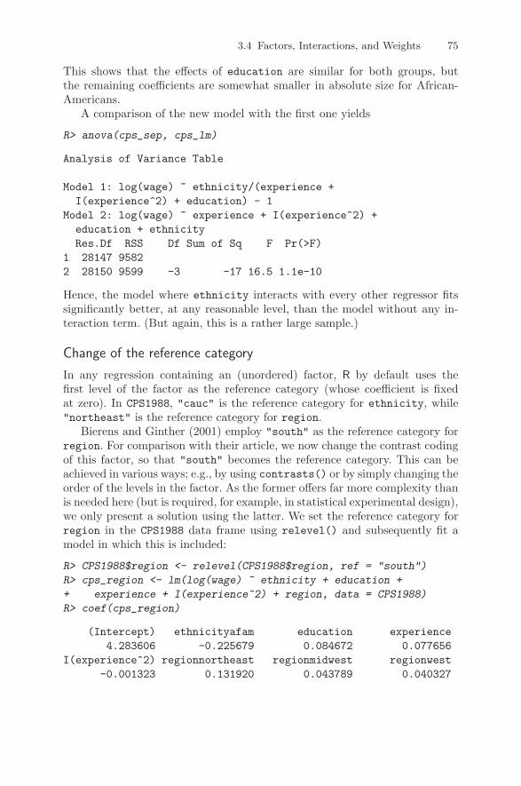
3.4 Factors, Interactions, and Weights 75

This shows that the effects of education are similar for both groups, butthe remaining coefficients are somewhat smaller in absolute size for African-Americans.

A comparison of the new model with the first one yields

R> anova(cps_sep, cps_lm)

Analysis of Variance Table

Model 1: log(wage) ~ ethnicity/(experience +I(experience^2) + education) - 1

Model 2: log(wage) ~ experience + I(experience^2) +education + ethnicityRes.Df RSS Df Sum of Sq F Pr(>F)

1 28147 95822 28150 9599 -3 -17 16.5 1.1e-10

Hence, the model where ethnicity interacts with every other regressor fitssignificantly better, at any reasonable level, than the model without any in-teraction term. (But again, this is a rather large sample.)

Change of the reference category

In any regression containing an (unordered) factor, R by default uses thefirst level of the factor as the reference category (whose coefficient is fixedat zero). In CPS1988, "cauc" is the reference category for ethnicity, while"northeast" is the reference category for region.

Bierens and Ginther (2001) employ "south" as the reference category forregion. For comparison with their article, we now change the contrast codingof this factor, so that "south" becomes the reference category. This can beachieved in various ways; e.g., by using contrasts() or by simply changing theorder of the levels in the factor. As the former offers far more complexity thanis needed here (but is required, for example, in statistical experimental design),we only present a solution using the latter. We set the reference category forregion in the CPS1988 data frame using relevel() and subsequently fit amodel in which this is included:

R> CPS1988$region <- relevel(CPS1988$region, ref = "south")

R> cps_region <- lm(log(wage) ~ ethnicity + education +

+ experience + I(experience^2) + region, data = CPS1988)

R> coef(cps_region)

(Intercept) ethnicityafam education experience4.283606 -0.225679 0.084672 0.077656

I(experience^2) regionnortheast regionmidwest regionwest-0.001323 0.131920 0.043789 0.040327

76 3 Linear Regression

Weighted least squares

Cross-section regressions are often plagued by heteroskedasticity. Diagnostictests against this alternative will be postponed to Chapter 4, but here weillustrate one of the remedies, weighted least squares (WLS), in an applicationto the journals data considered in Section 3.1. The reason is that lm() canalso handle weights.

Readers will have noted that the upper left plot of Figure 3.3 alreadyindicates that heteroskedasticity is a problem with these data. A possiblesolution is to specify a model of conditional heteroskedasticity, e.g.

E(ε2i |xi, zi) = g(z>i γ),

where g, the skedastic function, is a nonlinear function that can take on onlypositive values, zi is an `-vector of observations on exogenous or predeterminedvariables, and γ is an `-vector of parameters.

Here, we illustrate the fitting of some popular specifications using the priceper citation as the variable zi. Recall that assuming E(ε2

i |xi, zi) = σ2z2i leads

to a regression of yi/zi on 1/zi and xi/zi. This means that the fitting criterionchanges from

∑ni=1(yi − β1 − β2xi)2 to

∑ni=1 z−2

i (yi − β1 − β2xi)2, i.e., eachterm is now weighted by z−2

i . The solutions β1, β2 of the new minimizationproblem are called the weighted least squares (WLS) estimates, a special caseof generalized least squares (GLS). In R, this model is fitted using

R> jour_wls1 <- lm(log(subs) ~ log(citeprice), data = journals,

+ weights = 1/citeprice^2)

Note that the weights are entered as they appear in the new fitting criterion.Similarly,

R> jour_wls2 <- lm(log(subs) ~ log(citeprice), data = journals,

+ weights = 1/citeprice)

yields a regression with weights of the form 1/zi. Figure 3.5 provides the OLSregression line along with the lines corresponding to the two WLS specifica-tions:

R> plot(log(subs) ~ log(citeprice), data = journals)

R> abline(jour_lm)

R> abline(jour_wls1, lwd = 2, lty = 2)

R> abline(jour_wls2, lwd = 2, lty = 3)

R> legend("bottomleft", c("OLS", "WLS1", "WLS2"),

+ lty = 1:3, lwd = 2, bty = "n")

More often than not, we are not sure as to which form of the skedasticfunction to use and would prefer to estimate it from the data. This leads tofeasible generalized least squares (FGLS).

In our case, the starting point could be

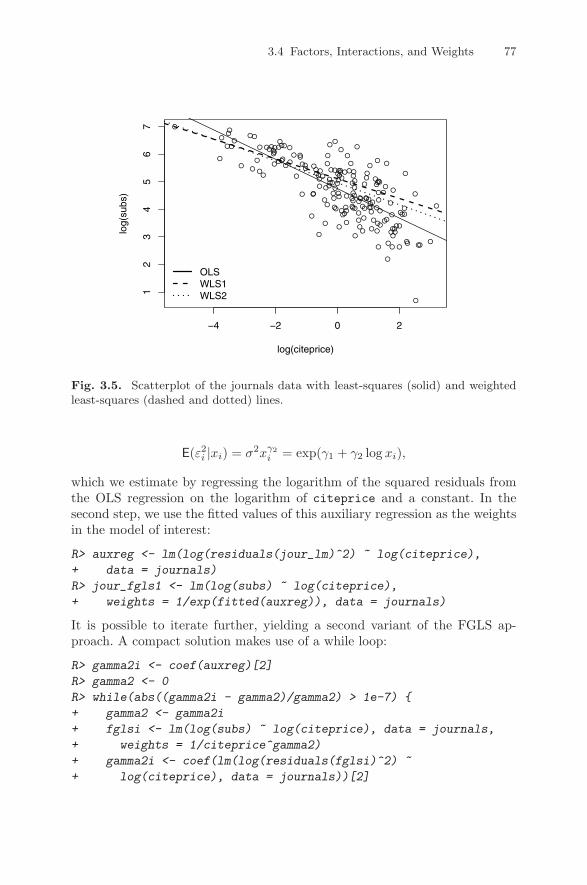
3.4 Factors, Interactions, and Weights 77

Fig. 3.5. Scatterplot of the journals data with least-squares (solid) and weightedleast-squares (dashed and dotted) lines.

E(ε2i |xi) = σ2xγ2

i = exp(γ1 + γ2 log xi),

which we estimate by regressing the logarithm of the squared residuals fromthe OLS regression on the logarithm of citeprice and a constant. In thesecond step, we use the fitted values of this auxiliary regression as the weightsin the model of interest:

R> auxreg <- lm(log(residuals(jour_lm)^2) ~ log(citeprice),

+ data = journals)

R> jour_fgls1 <- lm(log(subs) ~ log(citeprice),

+ weights = 1/exp(fitted(auxreg)), data = journals)

It is possible to iterate further, yielding a second variant of the FGLS ap-proach. A compact solution makes use of a while loop:

R> gamma2i <- coef(auxreg)[2]

R> gamma2 <- 0

R> while(abs((gamma2i - gamma2)/gamma2) > 1e-7)

+ gamma2 <- gamma2i

+ fglsi <- lm(log(subs) ~ log(citeprice), data = journals,

+ weights = 1/citeprice^gamma2)

+ gamma2i <- coef(lm(log(residuals(fglsi)^2) ~

+ log(citeprice), data = journals))[2]

−4 −2 0 2

12

34

56

7

log(citeprice)

log(

subs

)

OLSWLS1WLS2

78 3 Linear Regression

Fig. 3.6. Scatterplot of the journals data with OLS (solid) and iterated FGLS(dashed) lines.

+

R> jour_fgls2 <- lm(log(subs) ~ log(citeprice), data = journals,

+ weights = 1/citeprice^gamma2)

This loop specifies that, as long as the relative change of the slope coefficientγ2 exceeds 10−7 in absolute value, the iteration is continued; that is, a newset of coefficients for the skedastic function is computed utilizing the residualsfrom a WLS regression that employs the skedastic function estimated in thepreceding step. The final estimate of the skedastic function resulting from thewhile loop is then used in a further WLS regression, whose coefficients arereferred to as iterated FGLS estimates. This approach yields

R> coef(jour_fgls2)

(Intercept) log(citeprice)4.7758 -0.5008

and the parameter gamma2 of the transformation equals 0.2538, quite distinctfrom our first attempts using a predetermined skedastic function.

Figure 3.6 provides the OLS regression line along with the line correspond-ing to the iterated FGLS estimator. We see that the iterated FGLS solutionis more similar to the OLS solution than to the various WLS specificationsconsidered before.

−4 −2 0 2

12

34

56

7

log(citeprice)

log(

subs

)

3.5 Linear Regression with Time Series Data 79

3.5 Linear Regression with Time Series Data

In econometrics, time series regressions are often fitted by OLS. Hence, inprinciple, they can be fitted like any other linear regression model using lm()if the data set is held in a “data.frame”. However, this is typically not thecase for time series data, which are more conveniently stored in one of R’stime series classes. An example is “ts”, which holds its data in a vector ormatrix plus some time series attributes (start, end, frequency). More detailedinformation on time series analysis in R is provided in Chapter 6. Here, it suf-fices to note that using lm() with “ts” series has two drawbacks: (1) for fittedvalues or residuals, the time series properties are by default not preserved,and (2) lags or differences cannot directly be specified in the model formula.

These problems can be tackled in different ways. The simplest solution is todo the additional computations “by hand”; i.e., to compute lags or differencesbefore calling lm(). Alternatively, the package dynlm (Zeileis 2008) providesthe function dynlm(), which tries to overcome the problems described above.1

It allows for formulas such as d(y) ~ L(d(y)) + L(x, 4), here describing aregression of the first differences of a variable y on its first difference laggedby one period and on the fourth lag of a variable x; i.e., yi − yi−1 = β1 +β2 (yi−1−yi−2)+β3 xi−4 +εi. This is an autoregressive distributed lag (ADL)model.

As an illustration, we will follow Greene (2003, Chapter 8) and consider dif-ferent forms for a consumption function based on quarterly US macroeconomicdata from 1950(1) through 2000(4) as provided in the data set USMacroG, a“ts”time series. For such objects, there exists a plot() method, here employedfor visualizing disposable income dpi and consumption (in billion USD) via

R> data("USMacroG")

R> plot(USMacroG[, c("dpi", "consumption")], lty = c(3, 1),

+ plot.type = "single", ylab = "")

R> legend("topleft", legend = c("income", "consumption"),

+ lty = c(3, 1), bty = "n")

The result is shown in Figure 3.7. Greene (2003) considers two models,

consumptioni = β1 + β2 dpii + β3 dpii−1 + εi

consumptioni = β1 + β2 dpii + β3 consumptioni−1 + εi.

In the former model, a distributed lag model, consumption responds tochanges in income only over two periods, while in the latter specification,an autoregressive distributed lag model, the effects of income changes per-sist due to the autoregressive specification. The models can be fitted to theUSMacroG data by dynlm() as follows:1 A different approach that also works for modeling functions other than lm() is

implemented in the package dyn (Grothendieck 2005).

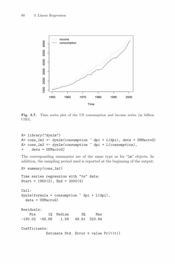
80 3 Linear Regression

Fig. 3.7. Time series plot of the US consumption and income series (in billionUSD).

R> library("dynlm")

R> cons_lm1 <- dynlm(consumption ~ dpi + L(dpi), data = USMacroG)

R> cons_lm2 <- dynlm(consumption ~ dpi + L(consumption),

+ data = USMacroG)

The corresponding summaries are of the same type as for “lm” objects. Inaddition, the sampling period used is reported at the beginning of the output:

R> summary(cons_lm1)

Time series regression with "ts" data:Start = 1950(2), End = 2000(4)

Call:dynlm(formula = consumption ~ dpi + L(dpi),data = USMacroG)

Residuals:Min 1Q Median 3Q Max

-190.02 -56.68 1.58 49.91 323.94

Coefficients:Estimate Std. Error t value Pr(>|t|)

Time

1950 1960 1970 1980 1990 2000

1000

2000

3000

4000

5000

6000

incomeconsumption

3.5 Linear Regression with Time Series Data 81

(Intercept) -81.0796 14.5081 -5.59 7.4e-08dpi 0.8912 0.2063 4.32 2.4e-05L(dpi) 0.0309 0.2075 0.15 0.88

Residual standard error: 87.6 on 200 degrees of freedomMultiple R-squared: 0.996, Adjusted R-squared: 0.996F-statistic: 2.79e+04 on 2 and 200 DF, p-value: <2e-16

The second model fits the data slightly better. Here only lagged consumptionbut not income is significant:

R> summary(cons_lm2)

Time series regression with "ts" data:Start = 1950(2), End = 2000(4)

Call:dynlm(formula = consumption ~ dpi + L(consumption),data = USMacroG)

Residuals:Min 1Q Median 3Q Max

-101.30 -9.67 1.14 12.69 45.32

Coefficients:Estimate Std. Error t value Pr(>|t|)

(Intercept) 0.53522 3.84517 0.14 0.89dpi -0.00406 0.01663 -0.24 0.81L(consumption) 1.01311 0.01816 55.79 <2e-16

Residual standard error: 21.5 on 200 degrees of freedomMultiple R-squared: 1, Adjusted R-squared: 1F-statistic: 4.63e+05 on 2 and 200 DF, p-value: <2e-16

The RSS of the first model can be obtained withdeviance(cons_lm1) and equals 1534001.49, and the RSS of the secondmodel, computed by deviance(cons_lm2), equals 92644.15. To visualize thesetwo fitted models, we employ time series plots of fitted values and residuals(see Figure 3.8) showing that the series of the residuals of cons_lm1 is some-what U-shaped, while that of cons_lm2 is closer to zero. To produce this plot,the following code was used:

R> plot(merge(as.zoo(USMacroG[,"consumption"]), fitted(cons_lm1),

+ fitted(cons_lm2), 0, residuals(cons_lm1),

+ residuals(cons_lm2)), screens = rep(1:2, c(3, 3)),

+ lty = rep(1:3, 2), ylab = c("Fitted values", "Residuals"),

+ xlab = "Time", main = "")

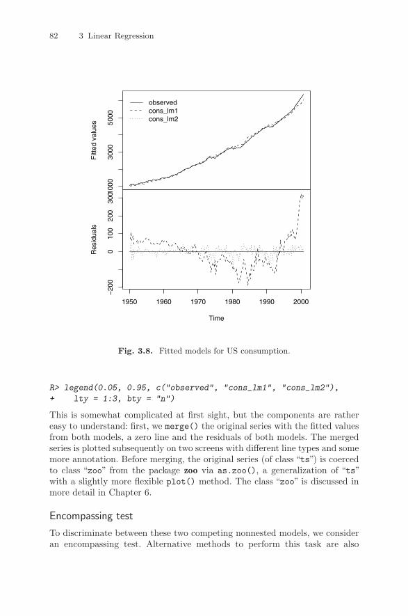
82 3 Linear Regression

Fig. 3.8. Fitted models for US consumption.

R> legend(0.05, 0.95, c("observed", "cons_lm1", "cons_lm2"),

+ lty = 1:3, bty = "n")

This is somewhat complicated at first sight, but the components are rathereasy to understand: first, we merge() the original series with the fitted valuesfrom both models, a zero line and the residuals of both models. The mergedseries is plotted subsequently on two screens with different line types and somemore annotation. Before merging, the original series (of class “ts”) is coercedto class “zoo” from the package zoo via as.zoo(), a generalization of “ts”with a slightly more flexible plot() method. The class “zoo” is discussed inmore detail in Chapter 6.

Encompassing test

To discriminate between these two competing nonnested models, we consideran encompassing test. Alternative methods to perform this task are also

Fitt

ed v

alue

s

1000

3000

5000

1950 1960 1970 1980 1990 2000

−20

00

100

200

300

Res

idua

ls

Time

observedcons_lm1cons_lm2

3.5 Linear Regression with Time Series Data 83

available; we consider the J test and the Cox test (see Davidson and MacKin-non 1981, 2004) in an exercise. All of these tests implement slightly differentapproaches to testing the same null hypotheses.

The encompassing approach to comparing two nonnested models is totransform the problem into a situation we can already deal with: comparingnested models. The idea is to fit the encompassing model comprising all regres-sors from both competing models, in our case the autoregressive distributedlag (ADL) model

R> cons_lmE <- dynlm(consumption ~ dpi + L(dpi) +

+ L(consumption), data = USMacroG)

and then to compare each of the two nonnested models with the encompassingmodel. Now if one of the models is not significantly worse than the encompass-ing model while the other is, this test would favor the former model over thelatter. As illustrated in the previous sections, nested models can be comparedwith anova(), and we can even carry out both tests of interest in one go:

R> anova(cons_lm1, cons_lmE, cons_lm2)

Analysis of Variance Table

Model 1: consumption ~ dpi + L(dpi)Model 2: consumption ~ dpi + L(dpi) + L(consumption)Model 3: consumption ~ dpi + L(consumption)Res.Df RSS Df Sum of Sq F Pr(>F)

1 200 15340012 199 73550 1 1460451 3951.4 < 2e-163 200 92644 -1 -19094 51.7 1.3e-11

The first F test compares the model cons_lm1 with the encompassing modelcons_lmE, and the second F test compares cons_lmE and cons_lm2. Bothmodels perform significantly worse compared with the encompassing model,although the F statistic is much smaller for cons_lm2.

Instead of computing the encompassing model by hand and then callinganova(), the function encomptest() from the lmtest package can be used.This simplifies the call to

R> encomptest(cons_lm1, cons_lm2)

Encompassing test

Model 1: consumption ~ dpi + L(dpi)Model 2: consumption ~ dpi + L(consumption)Model E: consumption ~ dpi + L(dpi) + L(consumption)

Res.Df Df F Pr(>F)M1 vs. ME 199 -1 3951.4 < 2e-16M2 vs. ME 199 -1 51.7 1.3e-11

84 3 Linear Regression

and leads to equivalent output. Internally, encomptest() relies on thewaldtest() function mentioned above.

3.6 Linear Regression with Panel Data

There has been considerable interest in panel data econometrics over the lasttwo decades, and hence it is almost mandatory to include a brief discussion ofsome common specifications in R. The package plm (Croissant and Millo 2008)contains the relevant fitting functions and methods. For the methodologicalbackground, we refer to Baltagi (2005).

Static linear models

For illustrating the basic fixed- and random-effects methods, we use the well-known Grunfeld data (Grunfeld 1958) comprising 20 annual observations onthe three variables real gross investment (invest), real value of the firm(value), and real value of the capital stock (capital) for 11 large US firmsfor the years 1935–1954. Originally employed in a study of the determinants ofcorporate investment in a University of Chicago Ph.D. thesis, these data havebeen a textbook classic since the 1970s. The accompanying package AER pro-vides the full data set comprising all 11 firms, and the documentation containsfurther details on alternative versions and errors therein.

The main difference between cross-sectional data and panel data is thatpanel data have an internal structure, indexed by a two-dimensional array,which must be communicated to the fitting function. We refer to the cross-sectional objects as “individuals” and the time identifier as “time”.

We use a subset of three firms for illustration and, utilizing plm.data(),tell R that the individuals are called "firm", whereas the time identifier iscalled "year":

R> data("Grunfeld", package = "AER")

R> library("plm")

R> gr <- subset(Grunfeld, firm %in% c("General Electric",

+ "General Motors", "IBM"))

R> pgr <- plm.data(gr, index = c("firm", "year"))

Instead of setting up a structured data frame pgr in advance, this could also bespecified on the fly in calls to plm() simply by supplying index = c("firm","year"). For later use, plain OLS on the pooled data is available using

R> gr_pool <- plm(invest ~ value + capital, data = pgr,

+ model = "pooling")

The basic one-way panel regression is

investit = β1valueit + β2capitalit + αi + νit, (3.3)

3.6 Linear Regression with Panel Data 85

where i = 1, . . . , n, t = 1, . . . , T , and the αi denote the individual-specificeffects.

A fixed-effects version is estimated by running OLS on a within-transformedmodel:

R> gr_fe <- plm(invest ~ value + capital, data = pgr,

+ model = "within")

R> summary(gr_fe)

Oneway (individual) effect Within Model

Call:plm(formula = invest ~ value + capital, data = pgr,model = "within")

Balanced Panel: n=3, T=20, N=60

Residuals :Min. 1st Qu. Median 3rd Qu. Max.

-167.00 -26.10 2.09 26.80 202.00

Coefficients :Estimate Std. Error t-value Pr(>|t|)

value 0.1049 0.0163 6.42 1.3e-10capital 0.3453 0.0244 14.16 < 2e-16

Total Sum of Squares: 1890000Residual Sum of Squares: 244000Multiple R-Squared: 0.871F-statistic: 185.407 on 55 and 2 DF, p-value: 0.00538

The summary provides a tabulation of observations per firm, here indicatingthat the data are balanced, as well as the usual regression output with coef-ficients (excluding the fixed effects) and associated standard errors and somemeasures of goodness of fit. A two-way model could have been estimated uponsetting effect = "twoways". If fixed effects need to be inspected, a fixef()method and an associated summary() method are available.

It is of interest to check whether the fixed effects are really needed. Thisis done by comparing the fixed effects and the pooled OLS fits by means ofpFtest() and yields

R> pFtest(gr_fe, gr_pool)

F test for effects

data: invest ~ value + capitalF = 56.82, df1 = 2, df2 = 55, p-value = 4.148e-14alternative hypothesis: significant effects

86 3 Linear Regression

indicating that there is substantial interfirm variation.It is also possible to fit a random-effects version of (3.3) using the same

fitting function upon setting model = "random" and selecting a method forestimating the variance components. Recall that a random-effects estimator isessentially an FGLS estimator, utilizing OLS after “quasi-demeaning” all vari-ables, where the precise form of the quasi-demeaning transformation dependson the random.method selected. Four methods are available: Swamy-Arora,Amemiya, Wallace-Hussain, and Nerlove (see, e.g., Baltagi 2005, for furtherinformation on these estimators). The default is random.method = "swar"(for Swamy-Arora), and for illustration we use random.method = "walhus"(for Wallace-Hussain) and obtain

R> gr_re <- plm(invest ~ value + capital, data = pgr,

+ model = "random", random.method = "walhus")

R> summary(gr_re)

Oneway (individual) effect Random Effect Model(Wallace-Hussain's transformation)

Call:plm(formula = invest ~ value + capital, data = pgr,model = "random", random.method = "walhus")

Balanced Panel: n=3, T=20, N=60

Effects:var std.dev share

idiosyncratic 4389.3 66.3 0.35individual 8079.7 89.9 0.65theta: 0.837

Residuals :Min. 1st Qu. Median 3rd Qu. Max.

-187.00 -32.90 6.96 31.40 210.00

Coefficients :Estimate Std. Error t-value Pr(>|t|)

(intercept) -109.9766 61.7014 -1.78 0.075value 0.1043 0.0150 6.95 3.6e-12capital 0.3448 0.0245 14.06 < 2e-16

Total Sum of Squares: 1990000Residual Sum of Squares: 258000Multiple R-Squared: 0.87F-statistic: 191.545 on 57 and 2 DF, p-value: 0.00521

3.6 Linear Regression with Panel Data 87

A comparison of the regression coefficients shows that fixed- and random-effects methods yield rather similar results for these data.

As was the case with the fixed-effects regression, it is of interest to checkwhether the random effects are really needed. Several versions of a Lagrangemultiplier test for this task are available in plmtest(), defaulting to the testproposed by Honda (1985). Here it yields

R> plmtest(gr_pool)

Lagrange Multiplier Test - (Honda)

data: invest ~ value + capitalnormal = 15.47, p-value < 2.2e-16alternative hypothesis: significant effects

This test also suggests that some form of parameter heterogeneity must betaken into account.

Random-effects methods are more efficient than the fixed-effects estima-tor under more restrictive assumptions, namely exogeneity of the individualeffects. It is therefore important to test for endogeneity, and the standard ap-proach employs a Hausman test. The relevant function phtest() requires twopanel regression objects, in our case yielding

R> phtest(gr_re, gr_fe)

Hausman Test

data: invest ~ value + capitalchisq = 0.0404, df = 2, p-value = 0.98alternative hypothesis: one model is inconsistent

In line with the rather similar estimates presented above, endogeneity doesnot appear to be a problem here.

plm contains methods for further types of static panel data models, no-tably the Hausman-Taylor model (Hausman and Taylor 1981) and varyingcoefficient models. We consider the Hausman-Taylor estimator in an exercise.

Dynamic linear models

To conclude this section, we present a more advanced example, the dynamicpanel data model

yit =p∑

j=1

%jyi,t−j + x>itβ + uit, uit = αi + βt + νit, (3.4)

estimated by the method of Arellano and Bond (1991). Recall that their esti-mator is a generalized method of moments (GMM) estimator utilizing laggedendogenous regressors after a first-differences transformation. plm comes with

88 3 Linear Regression

the original Arellano-Bond data (EmplUK) dealing with determinants of em-ployment (emp) in a panel of 140 UK firms for the years 1976–1984. The dataare unbalanced, with seven to nine observations per firm.

To simplify the exposition, we first set up a static formula containing therelevant variables average annual wage per employee (wage), the book value ofgross fixed assets (capital), and an index of value-added output at constantfactor cost (output), all in logarithms:

R> data("EmplUK", package = "plm")

R> form <- log(emp) ~ log(wage) + log(capital) + log(output)

The function providing the Arellano-Bond estimator is pgmm(), and it takes asits first argument a so-called dynformula, this being a static model equation,as given above, augmented with a list of integers containing the number oflags for each variable. The dynamic employment equation from Arellano andBond (1991) is now estimated as follows:

R> empl_ab <- pgmm(dynformula(form, list(2, 1, 0, 1)),

+ data = EmplUK, index = c("firm", "year"),

+ effect = "twoways", model = "twosteps",

+ gmm.inst = ~ log(emp), lag.gmm = list(c(2, 99)))

Hence, this is a dynamic model with p = 2 lagged endogenous terms (comparethis with Equation (3.4)) in which both log(wage) and log(output) occur upto lag 1, while for log(capital) only the contemporaneous term is included.A model containing time as well as firm-specific effects is specified, the instru-ments are lagged terms of the dependent variable log(emp), and the lags usedare given by the argument lag.gmm = list(c(2, 99)), indicating that alllags beyond lag 1 are to be used as instruments. This results in

R> summary(empl_ab)

Twoways effects Two steps model

Call:pgmm(formula = log(emp) ~ lag(log(emp), 1) + lag(log(emp),2) + log(wage) + lag(log(wage), 1) + log(capital) +log(output) + lag(log(output), 1), data = EmplUK,effect = "twoways", model = "twosteps",gmm.inst = ~log(emp), lag.gmm = list(c(2, 99)),index = c("firm", "year"))

Unbalanced Panel: n=140, T=7-9, N=1031

Number of Observations Used: 611

3.7 Systems of Linear Equations 89

ResidualsMin. 1st Qu. Median Mean 3rd Qu. Max.

-0.619000 -0.049500 -0.000457 -0.000184 0.053400 0.641000

CoefficientsEstimate Std. Error z-value Pr(>|z|)

lag(log(emp), 1) 0.4742 0.0853 5.56 2.7e-08lag(log(emp), 2) -0.0530 0.0273 -1.94 0.05222log(wage) -0.5132 0.0493 -10.40 < 2e-16lag(log(wage), 1) 0.2246 0.0801 2.81 0.00502log(capital) 0.2927 0.0395 7.42 1.2e-13log(output) 0.6098 0.1085 5.62 1.9e-08lag(log(output), 1) -0.4464 0.1248 -3.58 0.00035

Sargan Test: chisq(25) = 30.11 (p.value=0.22)Autocorrelation test (1): normal = -2.428 (p.value=0.0076)Autocorrelation test (2): normal = -0.3325 (p.value=0.37)Wald test for coefficients: chisq(7) = 372 (p.value=<2e-16)Wald test for time dummies: chisq(6) = 26.90 (p.value=0.000151)

suggesting that autoregressive dynamics are important for these data. Thetests at the bottom of the output indicate that the model is not fully satis-factory, but we refrain from presenting Arellano and Bond’s preferred specifi-cation, which in addition treats wages and capital as endogenous.

Note that, due to constructing lags and taking first differences, three crosssections are lost; hence the estimation period is 1979–1984 and only 611 ob-servations are effectively available for estimation.

3.7 Systems of Linear Equations

Systems of regression equations have been a hallmark of econometrics for sev-eral decades. Standard examples include seemingly unrelated regressions andvarious macroeconomic simultaneous equation models. The package systemfit(Henningsen and Hamann 2007) can estimate a number of multiple-equationmodels. As an example, we present a seemingly unrelated regression (SUR)model (Zellner 1962) for the Grunfeld data. As noted by Greene (2003, p. 329,fn. 39), “[a]lthough admittedly not current, these data are unusually cooper-ative for illustrating the different aspects of estimating systems of regressionequations”. Unlike the panel data models considered in the preceding section,which permit only individual-specific intercepts, the SUR model also allowsfor individual-specific slopes. (As regards terminology, the “individuals” of thepreceding section will now be referred to as “equations”.) The model assumescontemporaneous correlation across equations, and thus joint estimation of allparameters is, in general, more efficient than OLS on each equation.

90 3 Linear Regression

The main fitting function is systemfit(). When fitting a SUR model,it requires a “plm.data” object containing the information on the internalstructure of the data. This is set up as in the preceding section utilizingplm.data() (to save space we only consider two firms):

R> library("systemfit")

R> gr2 <- subset(Grunfeld, firm %in% c("Chrysler", "IBM"))

R> pgr2 <- plm.data(gr2, c("firm", "year"))

The main arguments to systemfit() are a formula, a data set, and a method(defaulting to "OLS"). Here we need method = "SUR":

R> gr_sur <- systemfit(invest ~ value + capital,

+ method = "SUR", data = pgr2)

R> summary(gr_sur, residCov = FALSE, equations = FALSE)

systemfit resultsmethod: SUR

N DF SSR detRCov OLS-R2 McElroy-R2system 40 34 4114 11022 0.929 0.927

N DF SSR MSE RMSE R2 Adj R2Chrysler 20 17 3002 176.6 13.29 0.913 0.903IBM 20 17 1112 65.4 8.09 0.952 0.946

Coefficients:Estimate Std. Error t value Pr(>|t|)

Chrysler_(Intercept) -5.7031 13.2774 -0.43 0.67293Chrysler_value 0.0780 0.0196 3.98 0.00096Chrysler_capital 0.3115 0.0287 10.85 4.6e-09IBM_(Intercept) -8.0908 4.5216 -1.79 0.09139IBM_value 0.1272 0.0306 4.16 0.00066IBM_capital 0.0966 0.0983 0.98 0.33951

Thus, summary() provides the standard regression results for each equationin a compact layout as well as some measures of overall fit. For compactness,we suppressed parts of the rather voluminous default output. Readers maywant to run this example with summary(gr_sur) to obtain more detailedinformation, including between-equation correlations.

The output indicates again that there is substantial variation among thefirms, and thus a single-equation model for the pooled data is not appropriate.

In addition to SUR models, systemfit can estimate linear simultaneous-equations models by several methods (two-stage least squares, three-stageleast squares, and variants thereof), and there is also a fitting function forcertain nonlinear specifications.

3.8 Exercises 91

3.8 Exercises

1. This exercise is taken from Faraway (2005, p. 23). Generate some artificialdata byx <- 1:20

y <- x + rnorm(20)

Fit a polynomial in x for predicting y. Compute β in two ways—by lm()and by using the direct calculation β = (X>X)−1X>y. At what degreeof polynomial does the direct calculation method fail? (Note the need forthe I() function in fitting the polynomial; e.g., in lm(y ~ x + I(x^2)).)(Lesson: Never use the textbook formula β = (X>X)−1X>y for compu-tations!)

2. Estimate a hedonic regression for the HousePrices data taken from Anglinand Gencay (1996), which contain prices of houses sold in the city ofWindsor, Canada, during July, August, and September 1987. These dataare also used in the textbook by Verbeek (2004).(a) Fit a multiple linear regression model to the logarithm of the price,

using all remaining variables as regressors. Experiment with modelscontaining lot size, number of bathrooms, number of bedrooms, andstories in logarithms and in levels, respectively. Which model do youprefer?

(b) What is the expected price of a two-story house of 4,700 sq. ft. withthree bedrooms, two bathrooms, a driveway, no recreational room, afull finished basement, without gas heating or air conditioning, andtwo-car garage, that is not located in a preferred area? Report also aprediction interval.

(c) In order to determine whether the logarithmic transformation of thedependent variable is really appropriate, a Box-Cox transformationmight be helpful. Use the function boxcox() from the package MASS.What do you conclude?

3. Consider the PSID1982 data from Cornwell and Rupert (1988) and dis-cussed further in Baltagi (2002).(a) Regress the logarithm of the wage on all available regressors plus ex-

perience squared.(b) Does gender interact with education and/or experience?

4. Section 3.5 considered two competing models for US consumption utiliz-ing an encompassing test. Different approaches to comparing nonnestedmodels are the J test suggested by Davidson and MacKinnon (1981) andthe Cox test. Both are available in the package lmtest in the functionsjtest() and coxtest(). For the methodological background, we refer toGreene (2003, Chapter 8) and Davidson and MacKinnon (2004).(a) Test cons_lm1 vs. cons_lm2 using the J test.(b) Test cons_lm1 vs. cons_lm2 using the Cox test.Do all tests lead to similar conclusions?

92 3 Linear Regression

5. Use the PSID1982 data and consider the following two nonnested models(compare with Baltagi 2002, p. 230):

M1 : log(wage) = β0 + β1education + β2experience + β3experience2

+β4weeks + β5married + β6gender

+β7ethnicity + β8union + ε

M2 : log(wage) = β0 + β1education + β2experience + β3experience2

+β4weeks + β5occupation + β6south

+β7smsa + β8industry + ν

(a) Compute the J tests for M1 vs. M2 and M2 vs. M1, respectively.(b) Both M1 and M2 can be artificially nested within a larger model. Use

an F test for M1 versus this augmented model. Repeat for M2 versusthe augmented model. What do you conclude?

6. The estimator of Hausman and Taylor (1981) is appropriate when onlysome of the individual effects in a panel regression are endogenous. Employthis estimator on a wage equation for the PSID1982 data using all 12regressors appearing in the preceding exercise. Note that you will have toenter all exogenous variables as instruments for themselves.(a) Consider the regressors experience, experience^2, occupation,

industry, union, and education as endogenous (as do Cornwell andRupert 1988).

(b) Consider the regressors experience, experience^2, weeks, married,union, and education as endogenous (as do Baltagi and Khanti-Akom1990; Baltagi 2005, Table 7.4).

(c) Which estimates do you consider more plausible?7. The function gls() from the package nlme will fit one of the classical

econometric regression models, the linear regression model yi = x>i β + εi

with AR(1) disturbances, εi = φεi−1 + νi, where νi ∼ (0, σ2ν) i.i.d. and

|φ| < 1, albeit by maximum likelihood, not by least-squares techniques.Select one of the firms from the Grunfeld data and estimate this model.What is the amount of first-order autocorrelation?

8. Find a way of estimating the SUR model from Section 3.7 using the plmpackage.

9. The function ivreg() from package AER will fit instrumental vari-able (IV) regressions. Using the USConsump1993 data taken from Baltagi(2002), estimate the simple Keynesian consumption function

expendituret = β0 + β1incomet + εt

(a) by OLS.(b) by IV. The only available instrument is investment, given by the

identity expenditure + investment = income.(c) Compare both sets of estimates using a Hausman test, thus replicating

Baltagi (2002, Section 11.7). What do you conclude?

4

Diagnostics and Alternative Methods ofRegression

The techniques presented in the preceding chapter tell only part of the storyof regression analysis. On the one hand, all of the estimates, tests, and othersummaries are computed as if the model and its assumptions were correct, buton the other, there exist various regression methods apart from OLS, some ofwhich are more appropriate in certain applications.

Here, we discuss several approaches to validating linear regression models:

• A popular approach (on occasion somewhat misleading) compares variousstatistics computed for the full data set with those obtained from deletingsingle observations. This is known as regression diagnostics.

• In econometrics, diagnostic tests have played a prominent role since about1980. The most important alternative hypotheses are heteroskedasticity,autocorrelation, and misspecification of the functional form.

• Also, the impenetrable disturbance structures typically present in obser-vational data have led to the development of “robust” covariance matrixestimators, a number of which have become available during the last 20years.

This chapter provides a brief introduction to all three approaches. It turnsout that graphical techniques are often quite effective at revealing structurethat one may not have suspected.

Furthermore, resistant (in the sense of resistance to outliers and unusualobservations) regression techniques are often quite helpful, although suchmethods do not appear to be as widely known among econometricians asthey deserve to be. We also include a brief introduction to quantile regression,a method that has been receiving increasing interest in applied econometrics,especially in labor economics.

C. Kleiber, A. Zeileis, Applied Econometrics with R,DOI: 10.1007/978-0-387-77318-6 4, © Springer Science+Business Media, LLC 2008

94 4 Diagnostics and Alternative Methods of Regression

4.1 Regression Diagnostics

There is extensive literature on examining the fit of linear regression models,mostly under the label “regression diagnostics”. The goal is to find points thatare not fitted as well as they should be or have undue influence on the fittingof the model. The techniques associated with Belsley, Kuh, and Welsch (1980)based on deletion of observations are widely available in statistical softwarepackages, and R is no exception.

This topic provides an excellent opportunity to further illustrate somebasic aspects of R programming, showing that variations on available functionsor plots are easily constructed with just a few lines of code. For illustration,we consider the PublicSchools data from the sandwich package, taken fromGreene (1993). They provide, for the 50 states of the United States of Americaand for Washington, DC, per capita Expenditure on public schools and percapita Income by state, all for the year 1979:

R> data("PublicSchools")

R> summary(PublicSchools)

Expenditure IncomeMin. :259 Min. : 57361st Qu.:315 1st Qu.: 6670Median :354 Median : 7597Mean :373 Mean : 76083rd Qu.:426 3rd Qu.: 8286Max. :821 Max. :10851NA's : 1

We first omit the incomplete observations using na.omit()—this affects onlyWisconsin, where Expenditure is not available. Subsequently, we generate ascatterplot with a fitted linear model, in which three observations are high-lighted:

R> ps <- na.omit(PublicSchools)

R> ps$Income <- ps$Income / 10000

R> plot(Expenditure ~ Income, data = ps, ylim = c(230, 830))

R> ps_lm <- lm(Expenditure ~ Income, data = ps)

R> abline(ps_lm)

R> id <- c(2, 24, 48)

R> text(ps[id, 2:1], rownames(ps)[id], pos = 1, xpd = TRUE)

The resulting plot in Figure 4.1 shows that there is a positive relationshipbetween expenditure and income; however, Alaska seems to be a dominantobservation in that it is far away from the bulk of the data. Two furtherobservations, Washington, DC, and Mississippi, also appear to deserve a closerlook. Visual inspection suggests that the OLS regression line is somewhattilted. We will pursue this issue below.

4.1 Regression Diagnostics 95

Fig. 4.1. Per capita expenditure on public schools versus per capita income.

The basic tool for examining the fit is the residuals, and we have alreadyseen that plot() applied to an “lm” object yields several diagnostic plots.Figure 4.2, resulting from

R> plot(ps_lm, which = 1:6)

depicts all six types (currently) available. The default is which = c(1:3,5);i.e., only four are shown.

Specifically, the first plot depicts residuals versus fitted values. It is usefulfor checking the assumption E(ε|X) = 0, and it brings out systematic varia-tions in the residuals that suggest that the model is incomplete. The tests andconfidence intervals used in summary(ps_lm) are based on the assumption ofi.i.d. normal errors. The residuals can be assessed for normality using a QQplot comparing the residuals to “ideal” normal observations. It plots the or-dered residuals against Φ−1 (i/(n + 1)), i = 1, . . . , n, where Φ−1 is the quantilefunction of the standard normal distribution. The third plot, a scale-locationplot, depicts

√|ri| (for the standardized residuals ri; see below for details)

against yi. It is useful for checking the assumption that errors are identicallydistributed, in particular that the variance is homogeneous, Var(ε|X) = σ2I.The remaining three plots display several combinations of standardized residu-als, leverage, and Cook’s distance—these diagnostic measures will be discussedin more detail below.

Thus, Figure 4.2 demonstrates that Alaska stands out in all plots: it has alarge residual (top left), and it therefore appears in the upper tail of the

0.6 0.7 0.8 0.9 1.0 1.1

300

400

500

600

700

800

Income

Exp

endi

ture

Alaska

Mississippi

Washington DC

96 4 Diagnostics and Alternative Methods of Regression

Fig. 4.2. Diagnostic plots for the public schools regression.

250 300 350 400 450 500 550 600

−10

00

100

200

Fitted values

Res

idua

ls

Residuals vs Fitted

Alaska

Nevada

Utah

−2 −1 0 1 2

−2

−1

01

23

4

Theoretical Quantiles

Sta

ndar

dize

d re

sidu

als

Normal Q−Q

Alaska

Washington DCNevada

250 300 350 400 450 500 550 600

0.0

0.5

1.0

1.5

2.0

Fitted values

Sta

ndar

dize

d re

sidu

als

Scale−LocationAlaska

Washington DCNevada

0 10 20 30 40 50

0.0

0.5

1.0

1.5

2.0

2.5

Obs. number

Coo

k's

dist

ance

Cook's distance

Alaska

Washington DC

Nevada

0.00 0.05 0.10 0.15 0.20

−2

−1

01

23

4

Leverage

Sta

ndar

dize

d re

sidu

als

Cook's distance1

0.5

0.5

1

Residuals vs Leverage

Alaska

Washington DCNevada

0.0

0.5

1.0

1.5

2.0

Leverage

Coo

k's

dist

ance

0 0.05 0.1 0.15 0.2

0

1

2

345Cook's distance vs Leverage

Alaska

Washington DC

Nevada

4.1 Regression Diagnostics 97

empirical distribution of the residuals (top right), it casts doubt on the as-sumption of homogeneous variances (middle left), it corresponds to an ex-traordinarily large Cook’s distance (middle and bottom right), and it has thehighest leverage (bottom left and right). There are further observations singledout, but none of these are as dominant as Alaska. Clearly, these observationsdeserve a closer look. To further explore the fit of our model, we briefly reviewregression diagnostics for linear models.

Leverage and standardized residuals

Recall that least-squares residuals are not independent and that they donot have the same variance. Specifically, if Var(ε|X) = σ2I, their variance-covariance matrix is Var(ε|X) = σ2(I−H), where H = X(X>X)−1X> is the“hat matrix”.

Basic diagnostics are the diagonal elements hii of H, which in R are pro-vided by the generic function hatvalues(). Since Var(εi|X) = σ2(1 − hii),observations with large values of hii will have small values of Var(εi|X), andhence residuals for such observations tend to be close to zero. Therefore, hii

is said to measure the leverage of the observation i. The trace of H is k (thenumber of regressors), and “large” is commonly taken to mean greater thantwo or three times the average element on the diagonal of H, k/n. Note thatthe value of hii depends only on X and not on y, and hence leverages containonly partial information about a point. This implies that there are two kindsof high-leverage points: “bad leverage points” and “good leverage points”. Theformer correspond to observations with large hii and unusual yi; such observa-tions can have a dramatic impact on the fit of a model. The latter correspondto observations with large hii and typical yi; such observations are beneficialbecause they improve the precision of the estimates.

Figure 4.3, obtained via

R> ps_hat <- hatvalues(ps_lm)

R> plot(ps_hat)

R> abline(h = c(1, 3) * mean(ps_hat), col = 2)

R> id <- which(ps_hat > 3 * mean(ps_hat))

R> text(id, ps_hat[id], rownames(ps)[id], pos = 1, xpd = TRUE)

depicts the diagonal elements of the hat matrix for the PublicSchools data.Var(εi|X) = σ2(1− hii) also suggests the use of

ri =εi

σ√

1− hii

.

The ri are the standardized residuals, available via rstandard() in R. (Theyare referred to as internally studentized residuals by some authors. This shouldnot be confused with the (externally) studentized residuals defined below.) Ifthe model assumptions are correct, Var(ri|X) = 1 and Cor(ri, rj |X) tends tobe small.

98 4 Diagnostics and Alternative Methods of Regression

Fig. 4.3. Diagonal elements of the hat matrix for the public schools data, withtheir mean and three times their mean as horizontal lines.

Deletion diagnostics

To detect unusual observations, Belsley et al. (1980) propose to compute var-ious leave-one-out (or deletion) diagnostics. Thus, one excludes point i andcomputes, for example, the estimates β(i) and σ(i), where the subscript (i) de-notes that observation i has been excluded. Similarly, y(i) = Xβ(i) denotes thevector of predictions of the yi utilizing β(i). Any observation whose removalfrom the data would cause a large change in the fit is considered “influential”.It may or may not have large leverage and may or may not be an outlier, butit will tend to have at least one of these properties.

Following Belsley et al. (1980), basic quantities are

DFFIT i = yi − yi,(i),

DFBETA = β − β(i),

COVRATIO i =det(σ2

(i)(X>(i)X(i))−1)

det(σ2(X>X)−1),

D2i =

(y − y(i))>(y − y(i))kσ2

.

Here, DFFIT measures the change in the fitted values, while DFBETA mea-sures the changes in the coefficients. COVRATIO considers the change in the

0 10 20 30 40 50

0.05

0.10

0.15

0.20

Index

ps_h

atAlaska

Washington DC

4.1 Regression Diagnostics 99

estimate of the OLS covariance matrix, while the D2i , the Cook’s distances (al-

ready encountered in the diagnostic plots in Figure 4.2), are especially popularbecause they reduce the information to a single value for each observation.Appropriately scaled versions of the first two quantities are called DFFITSand DFBETAS .

All these objects are available in the corresponding R functions dffit(),dffits(), dfbeta(), dfbetas(), covratio(), and cooks.distance(). Inaddition, the function rstudent() provides the (externally) studentized resid-uals

ti =εi

σ(i)

√1− hii

alluded to above.

The function influence.measures()

Fortunately, it is not necessary to compute all the preceding quantitiesseparately (although this is possible). R provides the convenience functioninfluence.measures(), which simultaneously calls dfbetas(), dffits(),covratio(), and cooks.distance(), returning a rectangular array of thesediagnostics. In addition, it highlights observations that are unusual for atleast one of the influence measures. Since the common influence measures arefunctions of ri and/or hii, which ones to choose is often a matter of taste.Since

R> influence.measures(ps_lm)

provides a rectangular array of size 50× 6, we do not show the result. Insteadwe briefly consider selected aspects.

With two regressors and 50 observations, the average diagonal element ofthe hat matrix is 0.04. The points with leverage higher than three times themean leverage can be obtained via

R> which(ps_hat > 3 * mean(ps_hat))

Alaska Washington DC2 48

This highlights Alaska and Washington, DC; for Alaska, the leverage is evenlarger than five times the mean (see Figure 4.3).

If the observations that are (potentially) influential according to at leastone criterion are desired, use

R> summary(influence.measures(ps_lm))

Potentially influential observations oflm(formula = Expenditure ~ Income, data = ps) :

100 4 Diagnostics and Alternative Methods of Regression

Fig. 4.4. Least-squares line with (solid) and without (dashed) Alaska, Mississippi,and Washington, DC.

dfb.1_ dfb.Incm dffit cov.r cook.d hatAlaska -2.39_* 2.52_* 2.65_* 0.55_* 2.31_* 0.21_*Mississippi 0.07 -0.07 0.08 1.14_* 0.00 0.08Washington DC 0.66 -0.71 -0.77_* 1.01 0.28 0.13_*

This again points us to Alaska and Washington, DC, and in addition Missis-sippi, which had been highlighted in Figure 4.1. It is noteworthy that Alaskastands out by any measure of influence. From Figure 4.4, resulting from

R> plot(Expenditure ~ Income, data = ps, ylim = c(230, 830))

R> abline(ps_lm)

R> id <- which(apply(influence.measures(ps_lm)$is.inf, 1, any))

R> text(ps[id, 2:1], rownames(ps)[id], pos = 1, xpd = TRUE)

R> ps_noinf <- lm(Expenditure ~ Income, data = ps[-id,])

R> abline(ps_noinf, lty = 2)

it is clear that this observation is a bad leverage point. To some extent, thisis also true for Washington, DC, but here the situation is not nearly as badas in the case of Alaska. The plot also depicts the least-squares line excludingthe three influential points, and it is obvious that it provides a much bettersummary of the data.

0.6 0.7 0.8 0.9 1.0 1.1

300

400

500

600

700

800

Income

Exp

endi

ture

Alaska

Mississippi

Washington DC

4.2 Diagnostic Tests 101

4.2 Diagnostic Tests

A more formal approach to validating regression models is diagnostic testing.Many cross-section regressions are plagued by heteroskedasticity. Similarly,regression models for time series data should be tested for residual autocor-relation. The package lmtest (Zeileis and Hothorn 2002), originally inspiredby the methods discussed in Kramer and Sonnberger (1986), provides a num-ber of tests for both alternatives plus further tests for misspecification of thefunctional form. A discussion of the underlying theory is provided in Baltagi(2002), Davidson and MacKinnon (2004), and Greene (2003), to mention afew sources. We proceed to the practical aspects of these procedures and referthe reader to these sources for the background formalities.

Almost all of the tests discussed below return an object of class “htest”(standing for hypothesis test), containing the value of the test statistic, thecorresponding p value, additional parameters such as degrees of freedom(where appropriate), the name of the tested model, and perhaps the methodused if there are several variants of the test.

For cross-section regressions, we return to the Journals data used in thepreceding chapter. As before, we set up a reduced data set journals thatalso contains the age of the journals (for the year 2000, when the data werecollected).

R> data("Journals")

R> journals <- Journals[, c("subs", "price")]

R> journals$citeprice <- Journals$price/Journals$citations

R> journals$age <- 2000 - Journals$foundingyear

As before, we consider a simple model that explains the logarithm of thenumber of library subscriptions for a journal by the logarithm of the price percitation.

R> jour_lm <- lm(log(subs) ~ log(citeprice), data = journals)

For a scatterplot of the data and the fitted model, we refer to Figure 3.1.

Testing for heteroskedasticity

For cross-section regressions, the assumption Var(εi|xi) = σ2 is typically indoubt. A popular test for checking this assumption is the Breusch-Pagan test(Breusch and Pagan 1979). It fits a linear regression model to the squaredresiduals ε2

i of the model under investigation and rejects if too much of thevariance is explained by the additional explanatory variables. For this auxiliaryregression, the same explanatory variables X are taken as in the main model.Other strategies could be to use the fitted values yi or the original regressorsplus squared terms and interactions (White 1980). For our model fitted to thejournals data, stored in jour_lm, the diagnostic plots in Figure 3.3 suggestthat the variance decreases with the fitted values or, equivalently, it increases

102 4 Diagnostics and Alternative Methods of Regression

with the price per citation. Hence, the regressor log(citeprice) used in themain model should also be employed for the auxiliary regression.

Under H0, the test statistic of the Breusch-Pagan test approximately fol-lows a χ2

q distribution, where q is the number of regressors in the auxiliaryregression (excluding the constant term). The textbook version of the test isfor normally distributed errors, an assumption that is often too strong forpractical work. It can be overcome by using a studentized version (Koenker1981).

The function bptest() implements all these flavors of the Breusch-Pagantest. By default, it computes the studentized statistic for the auxiliary regres-sion utilizing the original regressors X. Hence

R> bptest(jour_lm)

studentized Breusch-Pagan test

data: jour_lmBP = 9.803, df = 1, p-value = 0.001742

uses log(citeprice) in the auxiliary regression and detects heteroskedastic-ity in the data with respect to the price per citation. Alternatively, the Whitetest picks up the heteroskedasticity. It uses the original regressors as well astheir squares and interactions in the auxiliary regression, which can be passedas a second formula to bptest(). Here, this reduces to

R> bptest(jour_lm, ~ log(citeprice) + I(log(citeprice)^2),

+ data = journals)

studentized Breusch-Pagan test

data: jour_lmBP = 10.91, df = 2, p-value = 0.004271

Another test for heteroskedasticity—nowadays probably more popular intextbooks than in applied work—is the Goldfeld-Quandt test (Goldfeld andQuandt 1965). Its simple idea is that after ordering the sample with respectto the variable explaining the heteroskedasticity (e.g., price per citation in ourexample), the variance at the beginning should be different from the varianceat the end of the sample. Hence, splitting the sample and comparing the meanresidual sum of squares before and after the split point via an F test shouldbe able to detect a change in the variance. However, there are few applicationswhere a meaningful split point is known in advance; hence, in the absence ofbetter alternatives, the center of the sample is often used. Occasionally, somecentral observations are omitted in order to improve the power. The functiongqtest() implements this test; by default, it assumes that the data are al-ready ordered, and it also uses the middle of the sample as the split pointwithout omitting any central observations.

4.2 Diagnostic Tests 103

In order to apply this test to the journals data, we order the observationswith respect to price per citation. This leads again to a highly significantresult that confirms the Breusch-Pagan analysis presented above:

R> gqtest(jour_lm, order.by = ~ citeprice, data = journals)

Goldfeld-Quandt test

data: jour_lmGQ = 1.703, df1 = 88, df2 = 88, p-value = 0.00665

Testing the functional form

The assumption E(ε|X) = 0 is crucial for consistency of the least-squares es-timator. A typical source for violation of this assumption is a misspecificationof the functional form; e.g., by omitting relevant variables. One strategy fortesting the functional form is to construct auxiliary variables and assess theirsignificance using a simple F test. This is what Ramsey’s RESET (regressionspecification error test; Ramsey 1969) does: it takes powers of the fitted valuesy and tests whether they have a significant influence when added to the re-gression model. Alternatively, powers of the original regressors or of the firstprincipal component of X can be used. All three versions are implementedin the function resettest(). It defaults to using second and third powers ofthe fitted values as auxiliary variables. With only one real regressor in themodel matrix X (excluding the intercept), all three strategies yield equivalentresults. Hence we use

R> resettest(jour_lm)

RESET test

data: jour_lmRESET = 1.441, df1 = 2, df2 = 176, p-value = 0.2395

to assess whether second and third powers of log(citeprice) can signifi-cantly improve the model. The result is clearly non-significant, and hence nomisspecification can be detected in this direction.

The rainbow test (Utts 1982) takes a different approach to testing thefunctional form. Its basic idea is that even a misspecified model might be ableto fit the data reasonably well in the “center” of the sample but might lack fitin the tails. Hence, the rainbow test fits a model to a subsample (typically themiddle 50%) and compares it with the model fitted to the full sample usingan F test. To determine the “middle”, the sample has to be ordered; e.g., bya regressor variable or by the Mahalanobis distance of the regressor vector xi

to the mean regressor. Both procedures are implemented (along with somefurther options for fine-tuning the choice of the subsample) in the functionraintest(). For the jour_lm model, we may use

104 4 Diagnostics and Alternative Methods of Regression

R> raintest(jour_lm, order.by = ~ age, data = journals)

Rainbow test

data: jour_lmRain = 1.774, df1 = 90, df2 = 88, p-value = 0.003741

This orders the journals data by age and assesses whether the model fit forthe 50% “middle-aged” journals is different from the fit comprising all jour-nals. This appears to be the case, signaling that the relationship between thenumber of subscriptions and the price per citation also depends on the ageof the journal. As we will see below, the reason seems to be that libraries arewilling to pay more for established journals.

Another diagnostic test that relies on ordering the sample prior to testingis the Harvey-Collier test (Harvey and Collier 1977). For the ordered sample,the test computes the recursive residuals (Brown, Durbin, and Evans 1975) ofthe fitted model. The recursive residuals are essentially standardized one-step-ahead prediction errors: the linear model is fitted to the first i−1 observations,and from this the ith observation is predicted and the corresponding resid-ual is computed and suitably standardized. If the model is correctly specified,the recursive residuals have mean zero, whereas the mean should significantlydiffer from zero if the ordering variable has an influence on the regression rela-tionship. Therefore, the Harvey-Collier test is a simple t test for zero mean; itis implemented in the function harvtest(). Applying this test to the journalsdata yields the following result:

R> harvtest(jour_lm, order.by = ~ age, data = journals)

Harvey-Collier test

data: jour_lmHC = 5.081, df = 177, p-value = 9.464e-07

This confirms the results from the rainbow test, emphasizing that the age ofthe journals has a significant influence on the regression relationship.

Testing for autocorrelation

Just as the disturbances in cross-section models are typically heteroskedastic,they are often affected by autocorrelation (or serial correlation) in time seriesregressions. Let us reconsider the first model for the US consumption functionfrom Section 3.5:

R> data("USMacroG")

R> consump1 <- dynlm(consumption ~ dpi + L(dpi),

+ data = USMacroG)

A classical testing procedure suggested for assessing autocorrelation in regres-sion relationships is the Durbin-Watson test (Durbin and Watson 1950). The

4.2 Diagnostic Tests 105

test statistic is computed as the ratio of the sum of the squared first differencesof the residuals (i.e., (εi− εi−1)2), and the residual sum of squares. Under thenull hypothesis of no autocorrelation, the test statistic should be in the vicin-ity of 2—under the alternative of positive autocorrelation, it typically is muchsmaller. The distribution under the null hypothesis is nonstandard: under theassumption of normally distributed errors, it can be represented as the dis-tribution of a linear combination of χ2 variables with weights depending onthe regressor matrix X. Many textbooks still recommend using tabulated up-per and lower bounds of critical values. The function dwtest() implements anexact procedure for computing the p value and also provides a normal approx-imation for sufficiently large samples (both depending on the regressor matrixX). The function can be easily applied to the fitted consumption function via

R> dwtest(consump1)

Durbin-Watson test

data: consump1DW = 0.0866, p-value < 2.2e-16alternative hypothesis: true autocorrelation is greater than 0

here detecting a highly significant positive autocorrelation, which confirms theresults from Section 3.5.

Further tests for autocorrelation, originally suggested for diagnostic check-ing of ARIMA models (see Chapter 6), are the Box-Pierce test (Box and Pierce1970) and a modified version, the Ljung-Box test (Ljung and Box 1978). Bothare implemented in the function Box.test() in base R (in the stats pack-age). The test statistics are (approximate) χ2 statistics based on estimatesof the autocorrelations up to order p: the Box-Pierce statistic is n times thesum of squared autocorrelations, and the Ljung-Box refinement weighs thesquared autocorrelation at lag j by (n + 2)/(n − j) (j = 1, . . . , p). The de-fault in Box.test() is to use the Box-Pierce version with p = 1. Unlike thediagnostic tests in lmtest, the function expects a series of residuals and notthe specification of a linear model as its primary argument. Here, we applythe Box-Ljung test to the residuals of consump1, which again yields a highlysignificant result.

R> Box.test(residuals(consump1), type = "Ljung-Box")

Box-Ljung test

data: residuals(consump1)X-squared = 176.1, df = 1, p-value < 2.2e-16

An alternative approach to assessing autocorrelation is the Breusch-Godfrey test (Breusch 1979; Godfrey 1978)—unlike the Durbin-Watson test,this also works in the presence of lagged dependent variables (see also Sec-tion 7.1). The Breusch-Godfrey test is an LM test against both AR(p) and

106 4 Diagnostics and Alternative Methods of Regression

MA(p) alternatives, computed by fitting an auxiliary regression that explainsthe residuals ε by the original regressors X augmented by the lagged residualsup to order p (εi−1, . . . , εi−p) (where zeros are used as starting values). Theresulting RSS is compared with the RSS of the original RSS in a χ2 (or F )test. Both versions are implemented in the function bgtest(). By default, ituses an order of p = 1. Here, we obtain

R> bgtest(consump1)

Breusch-Godfrey test for serial correlation of order 1

data: consump1LM test = 193.0, df = 1, p-value < 2.2e-16

again confirming the previous results for this model.More details on various time series models in R and dealing with autocor-

relation are provided in Chapter 6.

4.3 Robust Standard Errors and Tests

As illustrated in the preceding sections, economic data typically exhibit someform of autocorrelation and/or heteroskedasticity. If the covariance structurewere known, it could be taken into account in a (parametric) model, but moreoften than not, the form of the autocorrelation or heteroskedasticity is un-known. In such cases, regression coefficients can typically still be estimatedconsistently using OLS (given that the functional form is correctly specified),but for valid inference a consistent covariance matrix estimate is essential.Over the last 20 years, several procedures for heteroskedasticity consistent(HC) and, more generally, for heteroskedasticity and autocorrelation consis-tent (HAC) covariance matrix estimation have been suggested in the econo-metrics literature. These are today routinely applied in econometric practice.

To be more specific, the problem is that the standard t and F testsperformed when calling summary() or anova() for a fitted linear model as-sume that errors are homoskedastic and uncorrelated given the regressors:Var(ε|X) = σ2I. In practice, however, as motivated for the data sets above,this is often not the case and Var(ε|X) = Ω, where Ω is unknown. In thissituation, the covariance matrix of the estimated regression coefficients β isgiven by

Var(β|X) =(X>X

)−1X>ΩX

(X>X

)−1,

which only reduces to the familiar σ2(X>X)−1 if the errors are indeed ho-moskedastic and uncorrelated. Hence, for valid inference in models with het-eroskedasticity and/or autocorrelation, it is vital to compute a robust esti-mate of Var(β|X). In R, the package sandwich (which is automatically at-tached when loading AER) provides the functions vcovHC() and vcovHAC()

4.3 Robust Standard Errors and Tests 107

implementing HC and HAC counterparts of vcov(). Furthermore, the es-timates produced by these functions can be easily plugged into the func-tions coeftest() and waldtest() from lmtest, functions generalizing thesummary() and anova() methods for fitted linear models. More details onthe implementation and application of these functions can be found in Zeileis(2004).

HC estimators

In cross-section regressions, it is typically appropriate to assume that Ω isa diagonal matrix with potentially non-constant diagonal entries. Therefore,a natural plug-in estimator for Var(β|X) could use Ω = diag(ω1, . . . , ωn);that is, a diagonal matrix. Various choices for ωi have been suggested in theliterature:

const : ωi = σ2

HC0 : ωi = ε2i

HC1 : ωi =n

n− kε2i

HC2 : ωi =ε2

i

1− hii

HC3 : ωi =ε2

i

(1− hii)2

HC4 : ωi =ε2

i

(1− hii)δi

where hii are again the diagonal elements of the hat matrix, h is theirmean, and δi = min4, hii/h. All these variants are available in the func-tion vcovHC().

The first version is the standard estimator for homoskedastic errors. Allothers produce different kinds of HC estimators. The estimator HC0 was in-troduced by Eicker (1963) and popularized in econometrics by White (1980).The estimators HC1, HC2, and HC3 were suggested by MacKinnon and White(1985) to improve the performance in small samples. A more extensive studyof small-sample behavior was conducted by Long and Ervin (2000), who arriveat the conclusion that HC3 provides the best performance in small samples,as it gives less weight to influential observations. HC3 is the default choice invcovHC(). More recently, Cribari-Neto (2004) suggested the estimator HC4to further improve small-sample performance, especially in the presence ofinfluential observations.

The function vcovHC() can be applied to a fitted linear model, just likethe function vcov(). For the model fitted to the journals data, both yieldrather similar estimates of the covariance matrix:

R> vcov(jour_lm)

108 4 Diagnostics and Alternative Methods of Regression

(Intercept) log(citeprice)(Intercept) 3.126e-03 -6.144e-05log(citeprice) -6.144e-05 1.268e-03

R> vcovHC(jour_lm)

(Intercept) log(citeprice)(Intercept) 0.003085 0.000693log(citeprice) 0.000693 0.001188

To obtain just the regression coefficients, their standard errors, and associatedt statistics (thus omitting the additional information on the fit of the modelprovided by summary(jour_lm)), the function call coeftest(jour_lm) maybe used. This has the advantage that other covariance matrix estimates—specified either as a function or directly as the fitted matrix—can be passedas an argument. For the journals data, this gives

R> coeftest(jour_lm, vcov = vcovHC)

t test of coefficients:

Estimate Std. Error t value Pr(>|t|)(Intercept) 4.7662 0.0555 85.8 <2e-16log(citeprice) -0.5331 0.0345 -15.5 <2e-16

which is almost identical to the standard summary() output. In the call above,the argument vcov was specified as a function; using coeftest(jour_lm,vcov = vcovHC(jour_lm)) (i.e., specifying vcov as the estimated covariancematrix ) yields identical output.

To compare the different types of HC estimators described above for thejournals data, we compute the corresponding standard errors for the fittedjour_lm model

R> t(sapply(c("const", "HC0", "HC1", "HC2", "HC3", "HC4"),

+ function(x) sqrt(diag(vcovHC(jour_lm, type = x)))))

(Intercept) log(citeprice)const 0.05591 0.03561HC0 0.05495 0.03377HC1 0.05526 0.03396HC2 0.05525 0.03412HC3 0.05555 0.03447HC4 0.05536 0.03459

which shows that, for these data, all estimators lead to almost identical results.In fact, all standard errors are slightly smaller than those computed under theassumption of homoskedastic errors.

To illustrate that using robust covariance matrix estimates can indeedmake a big difference, we reconsider the public schools data. We have already

4.3 Robust Standard Errors and Tests 109

fitted a linear regression model explaining the per capita public school ex-penditures by per capita income and detected several influential observations(most notably Alaska). This has the effect that if a quadratic model is fittedto the data, it appears to provide a significant improvement over the linearmodel, although this spurious significance is in fact only caused by a singleoutlier, Alaska:

R> ps_lm <- lm(Expenditure ~ Income, data = ps)

R> ps_lm2 <- lm(Expenditure ~ Income + I(Income^2), data = ps)

R> anova(ps_lm, ps_lm2)

Analysis of Variance Table

Model 1: Expenditure ~ IncomeModel 2: Expenditure ~ Income + I(Income^2)Res.Df RSS Df Sum of Sq F Pr(>F)

1 48 1810152 47 150986 1 30030 9.35 0.0037

As illustrated by Cribari-Neto (2004), this can be remedied by using a robustcovariance matrix estimate for inference. Note that in this context the patternin the residuals is typically not referred to as heteroskedasticity but rather ashaving outliers or influential observations. However, the principles underlyingthe HC estimators also yield appropriate results in this situation.

To obtain the same type of test as in the anova() call above, we usewaldtest(). This function provides a vcov argument, which again takes eithera function or a matrix. In the latter case, the covariance matrix has to becomputed for the more complex model to yield the correct result:

R> waldtest(ps_lm, ps_lm2, vcov = vcovHC(ps_lm2, type = "HC4"))

Wald test

Model 1: Expenditure ~ IncomeModel 2: Expenditure ~ Income + I(Income^2)Res.Df Df F Pr(>F)

1 482 47 1 0.08 0.77

This shows that the quadratic term is, in fact, not significant; an equivalentresult can also be obtained via coeftest(ps_lm2, vcov = vcovHC(ps_lm2,type = "HC4")).

HAC estimators

In time series regressions, if the error terms εi are correlated, Ω is not diago-nal and can only be estimated directly upon introducing further assumptions

110 4 Diagnostics and Alternative Methods of Regression

on its structure. However, if the form of heteroskedasticity and autocorrela-tion is unknown, valid standard errors and tests may be obtained by employ-ing empirical counterparts of X>ΩX instead. This is achieved by computingweighted sums of the empirical autocorrelations of εixi.

Various estimators that differ with respect to the choice of the weightshave been suggested. They have in common that weights are chosen accord-ing to some kernel function but differ in the choice of the kernel as well asthe choice of the bandwidth used. The function vcovHAC() implements a gen-eral framework for this type of estimator; more details on its implementationcan be found in Zeileis (2004). In addition to vcovHAC(), there are severalconvenience functions available in sandwich that make different strategies forchoosing kernels and bandwidths easily accessible: the function NeweyWest()implements the estimator of Newey and West (1987, 1994) using a nonpara-metric bandwidth selection, kernHAC() provides the class of kernel HAC es-timators of Andrews (1991) with parametric bandwidth selection as well asprewhitening, as suggested by Andrews and Monahan (1992), and weave()implements the class of weighted empirical adaptive variance estimators ofLumley and Heagerty (1999). In econometrics, the former two estimators arefrequently used, and here we illustrate how they can be applied to the con-sumption function consump1.

We compute the standard errors under the assumption of spherical errorsand compare them with the results of the quadratic spectral kernel and theBartlett kernel HAC estimators, both using prewhitening:

R> rbind(SE = sqrt(diag(vcov(consump1))),

+ QS = sqrt(diag(kernHAC(consump1))),

+ NW = sqrt(diag(NeweyWest(consump1))))

(Intercept) dpi L(dpi)SE 14.51 0.2063 0.2075QS 94.11 0.3893 0.3669NW 100.83 0.4230 0.3989

Both sets of robust standard errors are rather similar (except maybe for theintercept) and much larger than the uncorrected standard errors. As alreadyillustrated above, these functions may again be passed to coeftest() orwaldtest() (and other inference functions).

4.4 Resistant Regression

Leave-one-out diagnostics, as presented in Section 4.1, are a popular means fordetecting unusual observations. However, such observations may “mask” eachother, meaning that there may be several cases of the same type, and henceconventional diagnostics will not be able to detect such problems. With low-dimensional data such as PublicSchools, we can always resort to plotting,

4.4 Resistant Regression 111

but the situation is much worse with high-dimensional data. A solution is touse robust regression techniques.

There are many procedures in statistics and econometrics labeled as “ro-bust”, among them the sandwich covariance estimators discussed in the pre-ceding section. In this section, “robust” means “resistant” regression; thatis, regression methods that can withstand alterations of a small percent-age of the data set (in more practical terms, the estimates are unaffectedby a certain percentage of outlying observations). The first regression es-timators with this property, the least median of squares (LMS) and leasttrimmed squares (LTS) estimators defined by arg minβ medi|yi − x>i β| andarg minβ

∑qi=1 ε2

i:n(β), respectively (Rousseeuw 1984), were studied in theearly 1980s. Here, ε2

i = |yi−x>i β|2 are the squared residuals and i : n denotesthat they are arranged in increasing order. It turned out that LTS is prefer-able, and we shall use this method below. For an applied account of robustregression techniques, we refer to Venables and Ripley (2002).

In econometrics, these methods appear to be not as widely used as theydeserve to be. Zaman, Rousseeuw, and Orhan (2001) report that a searchthrough ECONLIT “led to a remarkably low total of 14 papers” publishedin the economics literature that rely on robust regression techniques. Thissection is an attempt at improving the situation.

For illustration, we consider a growth regression. The determinants of eco-nomic growth have been a popular field of empirical research for the last 20years. The starting point is the classical Solow model relating GDP growthto the accumulation of physical capital and to population growth. In an influ-ential paper, Mankiw, Romer, and Weil (1992) consider an augmented Solowmodel that also includes a proxy for the accumulation of human capital. Fora data set comprising 98 countries (available as GrowthDJ in AER), they con-clude that human capital is an important determinant of economic growth.They also note that the OECD countries are not fitted well by their model.This led Nonneman and Vanhoudt (1996) to reexamine their findings forOECD countries (available as OECDGrowth in AER), suggesting, among otherthings, a further extension of the Solow model by incorporating a measure ofaccumulation of technological know-how.

Here, we consider the classical textbook Solow model for the Nonnemanand Vanhoudt (1996) data with

log(Yt/Y0) = β1 + β2 log(Y0) + β3 log(Kt) + β4 log(nt + 0.05) + εt,

where Yt and Y0 are real GDP in periods t and 0, respectively, Kt is a measureof the accumulation of physical capital, and nt is population growth (with 5%added in order to account for labor productivity growth). The OECDGrowthdata provide these variables for all OECD countries with a population exceed-ing 1 million. Specifically, Yt and Y0 are taken as the real GDP (per person ofworking age; i.e., ages 15 to 65) in 1985 and 1960, respectively, both in 1985international prices, Kt is the average of the annual ratios of real domestic

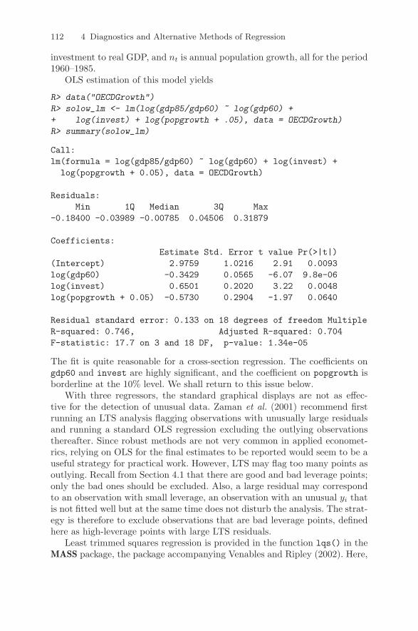
112 4 Diagnostics and Alternative Methods of Regression

investment to real GDP, and nt is annual population growth, all for the period1960–1985.

OLS estimation of this model yields

R> data("OECDGrowth")

R> solow_lm <- lm(log(gdp85/gdp60) ~ log(gdp60) +

+ log(invest) + log(popgrowth + .05), data = OECDGrowth)

R> summary(solow_lm)

Call:lm(formula = log(gdp85/gdp60) ~ log(gdp60) + log(invest) +log(popgrowth + 0.05), data = OECDGrowth)

Residuals:Min 1Q Median 3Q Max

-0.18400 -0.03989 -0.00785 0.04506 0.31879

Coefficients:Estimate Std. Error t value Pr(>|t|)

(Intercept) 2.9759 1.0216 2.91 0.0093log(gdp60) -0.3429 0.0565 -6.07 9.8e-06log(invest) 0.6501 0.2020 3.22 0.0048log(popgrowth + 0.05) -0.5730 0.2904 -1.97 0.0640

Residual standard error: 0.133 on 18 degrees of freedom MultipleR-squared: 0.746, Adjusted R-squared: 0.704F-statistic: 17.7 on 3 and 18 DF, p-value: 1.34e-05

The fit is quite reasonable for a cross-section regression. The coefficients ongdp60 and invest are highly significant, and the coefficient on popgrowth isborderline at the 10% level. We shall return to this issue below.

With three regressors, the standard graphical displays are not as effec-tive for the detection of unusual data. Zaman et al. (2001) recommend firstrunning an LTS analysis flagging observations with unusually large residualsand running a standard OLS regression excluding the outlying observationsthereafter. Since robust methods are not very common in applied economet-rics, relying on OLS for the final estimates to be reported would seem to be auseful strategy for practical work. However, LTS may flag too many points asoutlying. Recall from Section 4.1 that there are good and bad leverage points;only the bad ones should be excluded. Also, a large residual may correspondto an observation with small leverage, an observation with an unusual yi thatis not fitted well but at the same time does not disturb the analysis. The strat-egy is therefore to exclude observations that are bad leverage points, definedhere as high-leverage points with large LTS residuals.

Least trimmed squares regression is provided in the function lqs() in theMASS package, the package accompanying Venables and Ripley (2002). Here,

4.4 Resistant Regression 113

lqs stands for least quantile of squares because lqs() also provides LMSregression and generalizations thereof. However, the default is LTS, which iswhat we use here.

The code chunk

R> library("MASS")

R> solow_lts <- lqs(log(gdp85/gdp60) ~ log(gdp60) +

+ log(invest) + log(popgrowth + .05), data = OECDGrowth,

+ psamp = 13, nsamp = "exact")

sets psamp = 13, and thus we trim 9 of the 22 observations in OECDGrowth. Bychoosing nsamp = "exact", the LTS estimates are computed by minimizingthe sum of squares from all conceivable subsamples of size 13. This is onlyfeasible for small samples such as the data under investigation; otherwise someother sampling technique should be used.1

lqs() provides two estimates of scale, the first defined via the fit criterionand the second based on the variance of those residuals whose absolute valueis less than 2.5 times the initial estimate. Following Zaman et al. (2001), weuse the second estimate of scale and define a large residual as a scaled residualexceeding 2.5 in absolute values. Thus, the observations corresponding to smallresiduals can be extracted by

R> smallresid <- which(

+ abs(residuals(solow_lts)/solow_lts$scale[2]) <= 2.5)

We still need a method for detecting the high-leverage points. For consis-tency, this method should be a robust method. The robustness literature pro-vides several robust covariance estimators that can be used to determine thesepoints, among them the minimum-volume ellipsoid (MVE) and the minimum-covariance determinant (MCD) methods. Both are implemented in the func-tion cov.rob() from the MASS package, with MVE being the default.

Below, we extract the model matrix, estimate its covariance matrix byMVE, and subsequently compute the leverage (utilizing the mahalanobis()function), storing the observations that are not high-leverage points.

R> X <- model.matrix(solow_lm)[,-1]

R> Xcv <- cov.rob(X, nsamp = "exact")

R> nohighlev <- which(

+ sqrt(mahalanobis(X, Xcv$center, Xcv$cov)) <= 2.5)

The“good observations”are defined as those having at least one of the desiredproperties, small residual or low leverage. They are determined by concate-nating the vectors smallresid and nohighlev and removing duplicates usingunique():

R> goodobs <- unique(c(smallresid, nohighlev))

1 Our results slightly improve on Zaman et al. (2001) because they do not seem tohave used an exhaustive search for determining their robust estimates.

114 4 Diagnostics and Alternative Methods of Regression

Thus, the “bad observations” are

R> rownames(OECDGrowth)[-goodobs]

[1] "Canada" "USA" "Turkey" "Australia"

Running OLS excluding the bad leverage points now yields

R> solow_rob <- update(solow_lm, subset = goodobs)

R> summary(solow_rob)

Call:lm(formula = log(gdp85/gdp60) ~ log(gdp60) + log(invest) +log(popgrowth + 0.05), data = OECDGrowth,subset = goodobs)

Residuals:Min 1Q Median 3Q Max

-0.1545 -0.0555 -0.0065 0.0316 0.2677

Coefficients:Estimate Std. Error t value Pr(>|t|)

(Intercept) 3.7764 1.2816 2.95 0.0106log(gdp60) -0.4507 0.0569 -7.93 1.5e-06log(invest) 0.7033 0.1906 3.69 0.0024log(popgrowth + 0.05) -0.6504 0.4190 -1.55 0.1429

Residual standard error: 0.107 on 14 degrees of freedomMultiple R-squared: 0.853, Adjusted R-squared: 0.822F-statistic: 27.1 on 3 and 14 DF, p-value: 4.3e-06

Note that the results are somewhat different from the original OLS results forthe full data set. Specifically, population growth does not seem to belong inthis model. Of course, this does not mean that population growth plays no rolein connection with economic growth but just that this variable is not neededconditional on the inclusion of the remaining ones and, more importantly, forthis subset of countries. With a larger set of countries, population growthis quite likely to play its role. The OECD countries are fairly homogeneouswith respect to that variable, and some countries with substantial populationgrowth have been excluded in the robust fit. Hence, the result should not comeas a surprise.

Augmented or extended versions of the Solow model that include furtherregressors such as human capital (log(school)) and technological know-how(log(randd)) are explored in an exercise.

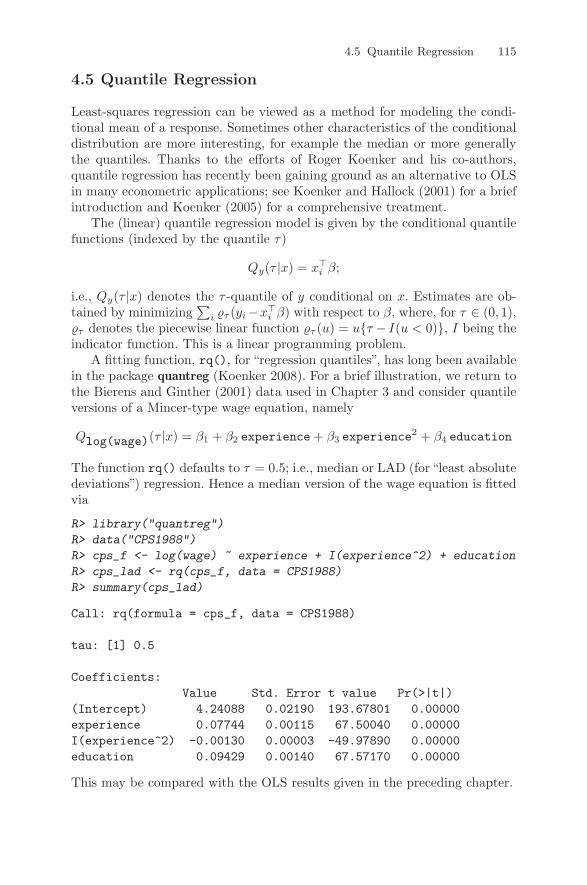
4.5 Quantile Regression 115

4.5 Quantile Regression

Least-squares regression can be viewed as a method for modeling the condi-tional mean of a response. Sometimes other characteristics of the conditionaldistribution are more interesting, for example the median or more generallythe quantiles. Thanks to the efforts of Roger Koenker and his co-authors,quantile regression has recently been gaining ground as an alternative to OLSin many econometric applications; see Koenker and Hallock (2001) for a briefintroduction and Koenker (2005) for a comprehensive treatment.

The (linear) quantile regression model is given by the conditional quantilefunctions (indexed by the quantile τ)

Qy(τ |x) = x>i β;

i.e., Qy(τ |x) denotes the τ -quantile of y conditional on x. Estimates are ob-tained by minimizing

∑i %τ (yi−x>i β) with respect to β, where, for τ ∈ (0, 1),

%τ denotes the piecewise linear function %τ (u) = uτ − I(u < 0), I being theindicator function. This is a linear programming problem.

A fitting function, rq(), for “regression quantiles”, has long been availablein the package quantreg (Koenker 2008). For a brief illustration, we return tothe Bierens and Ginther (2001) data used in Chapter 3 and consider quantileversions of a Mincer-type wage equation, namely

Qlog(wage)(τ |x) = β1 + β2 experience + β3 experience2 + β4 education

The function rq() defaults to τ = 0.5; i.e., median or LAD (for“least absolutedeviations”) regression. Hence a median version of the wage equation is fittedvia

R> library("quantreg")

R> data("CPS1988")

R> cps_f <- log(wage) ~ experience + I(experience^2) + education

R> cps_lad <- rq(cps_f, data = CPS1988)

R> summary(cps_lad)

Call: rq(formula = cps_f, data = CPS1988)

tau: [1] 0.5

Coefficients:Value Std. Error t value Pr(>|t|)

(Intercept) 4.24088 0.02190 193.67801 0.00000experience 0.07744 0.00115 67.50040 0.00000I(experience^2) -0.00130 0.00003 -49.97890 0.00000education 0.09429 0.00140 67.57170 0.00000

This may be compared with the OLS results given in the preceding chapter.

116 4 Diagnostics and Alternative Methods of Regression

Quantile regression is particularly useful when modeling several quantilessimultaneously. In order to illustrate some basic functions from quantreg, weconsider the first and third quartiles (i.e., τ = 0.25 and τ = 0.75). Since rq()takes vectors of quantiles, fitting these two models is as easy as

R> cps_rq <- rq(cps_f, tau = c(0.25, 0.75), data = CPS1988)

R> summary(cps_rq)

Call: rq(formula = cps_f, tau = c(0.25, 0.75), data = CPS1988)

tau: [1] 0.25

Coefficients:Value Std. Error t value Pr(>|t|)

(Intercept) 3.78227 0.02866 131.95187 0.00000experience 0.09156 0.00152 60.26473 0.00000I(experience^2) -0.00164 0.00004 -45.39064 0.00000education 0.09321 0.00185 50.32519 0.00000

Call: rq(formula = cps_f, tau = c(0.25, 0.75), data = CPS1988)

tau: [1] 0.75

Coefficients:Value Std. Error t value Pr(>|t|)

(Intercept) 4.66005 0.02023 230.39729 0.00000experience 0.06377 0.00097 65.41363 0.00000I(experience^2) -0.00099 0.00002 -44.15591 0.00000education 0.09434 0.00134 70.65853 0.00000

A natural question is whether the regression lines or surfaces are parallel; i.e.,whether the effects of the regressors are uniform across quantiles. There existsan anova() method for exploring this question. It requires separate fits foreach quantile and can be used in two forms: for an overall test of equality ofthe entire sets of coefficients, we use

R> cps_rq25 <- rq(cps_f, tau = 0.25, data = CPS1988)

R> cps_rq75 <- rq(cps_f, tau = 0.75, data = CPS1988)

R> anova(cps_rq25, cps_rq75)

Quantile Regression Analysis of Variance Table

Model: log(wage) ~ experience + I(experience^2) + educationJoint Test of Equality of Slopes: tau in 0.25 0.75

Df Resid Df F value Pr(>F)1 3 56307 115 <2e-16

4.5 Quantile Regression 117

while

R> anova(cps_rq25, cps_rq75, joint = FALSE)

Quantile Regression Analysis of Variance Table

Model: log(wage) ~ experience + I(experience^2) + educationTests of Equality of Distinct Slopes: tau in 0.25 0.75

Df Resid Df F value Pr(>F)experience 1 56309 339.41 <2e-16I(experience^2) 1 56309 329.74 <2e-16education 1 56309 0.35 0.55

provides coefficient-wise comparisons. We see that effects are not uniformacross quantiles in this example, with differences being associated with theregressor experience.

It is illuminating to visualize the results from quantile regression fits. Onepossibility is to plot, for each regressor, the estimate as a function of thequantile. This is achieved using plot() on the summary() of the quantileregression object. In order to obtain a more meaningful plot, we now use alarger set of τs, specifically τ ∈ 0.05, 0.1, . . . , 0.95:

R> cps_rqbig <- rq(cps_f, tau = seq(0.05, 0.95, by = 0.05),

+ data = CPS1988)

R> cps_rqbigs <- summary(cps_rqbig)

Figure 4.5, obtained via

R> plot(cps_rqbigs)

visualizes the variation of the coefficients as a function of τ , and it is clear thatthe influence of the covariates is far from uniform. The shaded areas representpointwise 90% (by default) confidence intervals for the quantile regressionestimates. For comparison, the horizontal solid and dashed lines shown ineach plot signify the OLS estimate and an associated 90% confidence interval.

It should be noted that quantreg contains a number of further functions forquantile modeling, including nonlinear and nonparametric versions. There alsoexist several algorithms for fitting these models (specifically, both exterior andinterior point methods) as well as several choices of methods for computingconfidence intervals and related test statistics.

118 4 Diagnostics and Alternative Methods of Regression

Fig. 4.5. Visualization of a quantile regression fit.

4.6 Exercises

1. Consider the CigarettesB data taken from Baltagi (2002). Run a re-gression of real per capita consumption on real price and real per capitaincome (all variables in logarithms). Obtain the usual diagnostic statis-tics using influence.measures(). Which observations are influential? Towhich states do they correspond? Are the results intuitive?

2. Reanalyze the PublicSchools data using robust methods:(a) Run a regression of Expenditure on Income using least trimmed

squares (LTS). Which observations correspond to large LTS residu-als?

(b) Which observations are high-leverage points?

0.2 0.4 0.6 0.8

3.5

4.0

4.5

5.0

(Intercept)

0.2 0.4 0.6 0.8

0.05

0.06

0.07

0.08

0.09

0.10

experience

0.2 0.4 0.6 0.8

−0.

0020

−0.

0016

−0.

0012

−0.

0008

I(experience^2)

0.2 0.4 0.6 0.8

0.07

0.08

0.09

education

4.6 Exercises 119

(c) Run OLS on the data, excluding all observations that have large LTSresiduals and are high-leverage points. Compare your result with theanalysis provided in Section 4.1.

3. Explore further growth regressions for the OECDGrowth data using the aug-mented and extended Solow models of Nonneman and Vanhoudt (1996),which consider the additional regressors log(school) (human capital)and log(randd) (technological know-how), respectively. First, replicatethe OLS results from Nonneman and Vanhoudt (1996, Table IV), andsubsequently compare them with the resistant LTS results by adoptingthe strategy of Zaman et al. (2001).

4. When discussing quantile regression, we confined ourselves to the standardMincer equation. However, the CPS1988 data contain further explanatoryvariables, namely the factors ethnicity, smsa, region, and parttime.Replicate the LAD regression (i.e., the quantile regression with τ = 0.5)results from Bierens and Ginther (2001) using these covariates.

5

Models of Microeconometrics

Many econometrics packages can perform the analyses discussed in the fol-lowing sections. Often, however, they do so with a different program or pro-cedure for each type of analysis—for example, probit regression and Poissonregression—so that the unifying structure of these methods is not apparent.

R does not come with different programs for probit and Poisson regressions.Instead, it follows mainstream statistics in providing the unifying frameworkof generalized linear models (GLMs) and a single fitting function, glm(). Fur-thermore, models extending GLMs are provided by R functions that analo-gously extend the basic glm() function (i.e., have similar interfaces, returnvalues, and associated methods).

This chapter begins with a brief introduction to GLMs, followed by sectionson regression for binary dependent variables, counts, and censored dependentvariables. The final section points to methods for multinomial and ordinalresponses and semiparametric extensions.

5.1 Generalized Linear Models

Chapter 3 was devoted to the linear regression model, for which inferenceis exact and the OLS estimator coincides with the maximum likelihood esti-mator (MLE) when the disturbances are, conditional on the regressors, i.i.d.N (0, σ2). Here, we briefly describe how the salient features of this model canbe extended to situations where the dependent variable y comes from a widerclass of distributions.

Three aspects of the linear regression model for a conditionally normallydistributed response y are:

1. The linear predictor ηi = x>i β through which µi = E(yi|xi) depends onthe k × 1 vectors xi of observations and β of parameters.

2. The distribution of the dependent variable yi|xi is N (µi, σ2).

3. The expected response is equal to the linear predictor, µi = ηi.

C. Kleiber, A. Zeileis, Applied Econometrics with R,DOI: 10.1007/978-0-387-77318-6 5, © Springer Science+Business Media, LLC 2008

122 5 Models of Microeconometrics

The class of generalized linear models (GLMs) extends 2. and 3. to moregeneral families of distributions for y and to more general relations betweenE(yi|xi) and the linear predictor than the identity. Specifically, yi|xi may nowfollow a density or probability mass function of the type

f(y; θ, φ) = exp

yθ − b(θ)φ

+ c(y;φ)

, (5.1)

where θ, called the canonical parameter, depends on the linear predictor, andthe additional parameter φ, called the dispersion parameter, is often known.Also, the linear predictor and the expectation of y are now related by a mono-tonic transformation,

g(µi) = ηi.

For fixed φ, (5.1) describes a linear exponential family, a class of distribu-tions that includes a number of well-known distributions such as the normal,Poisson, and binomial.

The class of generalized linear models is thus defined by the followingelements:

1. The linear predictor ηi = x>i β through which µi = E(yi|xi) depends onthe k × 1 vectors xi of observations and β of parameters.

2. The distribution of the dependent variable yi|xi is a linear exponentialfamily.

3. The expected response and the linear predictor are related by a monotonictransformation, g(µi) = ηi, called the link function of the GLM.

Thus, the family of GLMs extends the applicability of linear-model ideasto data where responses are binary or counts, among further possibilities. Theunifying framework of GLMs emerged in the statistical literature in the early1970s (Nelder and Wedderburn 1972).

The Poisson distribution with parameter µ and probability mass function

f(y;µ) =e−µµy

y!, y = 0, 1, 2, . . . ,

perhaps provides the simplest example leading to a nonnormal GLM. Writing

f(y;µ) = exp(y log µ− µ− log y!),

it follows that the Poisson density has the form (5.1) with θ = log µ, b(θ) = eθ,φ = 1, and c(y;φ) = − log y!. Furthermore, in view of E(y) = µ > 0, it isnatural to employ log µ = η; i.e., to use a logarithmic link. The transformationg relating the original parameter, here µ, and the canonical parameter θ fromthe exponential family representation is called the canonical link in the GLMliterature. Hence the logarithmic link is in fact the canonical link for thePoisson family.

5.2 Binary Dependent Variables 123

Table 5.1. Selected GLM families and their canonical (default) links.

Family Canonical link Name

binomial logµ/(1− µ) logit

gaussian µ identity

poisson log µ log

Similarly, for binary data, the Bernoulli distribution (a special case of thebinomial distribution) is suitable, and here we have

f(y; p) =

y log(

p

1− p

)+ log(1− p)

, y ∈ 0, 1,

which shows that the logit transform logp/(1− p), the quantile function ofthe logistic distribution, corresponds to the canonical link for the binary re-gression model. A widely used non-canonical link for this model is the quantilefunction of the standard normal distribution, yielding the probit link.

Table 5.1 provides a summary of the most important examples of general-ized linear models. A more complete list may be found in standard referenceson GLMs such as McCullagh and Nelder (1989).

In view of the built-in distributional assumption, it is natural to estimatea GLM by the method of maximum likelihood. For the GLM with a normallydistributed response and the identity link, the MLE reduces to the least-squares estimator and is therefore available in closed form. In general, thereis no closed-form expression for the MLE; instead it must be determined us-ing numerical methods. For GLMs, the standard algorithm is called iterativeweighted least squares (IWLS). It is an implementation of the familiar Fisherscoring algorithm adapted for GLMs.

These analogies with the classical linear model suggest that a fitting func-tion for GLMs could look almost like the fitting function for the linear model,lm(). In R, this is indeed the case. The fitting function for GLMs is calledglm(), and its syntax closely resembles the syntax of lm(). Of course, there areextra arguments for selecting the response distribution and the link function,but apart from this, the familiar arguments such as formula, data, weights,and subset are all available. In addition, all the extractor functions from Ta-ble 3.1 have methods for objects of class “glm”, the class of objects returnedby glm().

5.2 Binary Dependent Variables

Regression problems with binary dependent variables are quite common inmicroeconometrics, usually under the names of logit and probit regressions.The model is

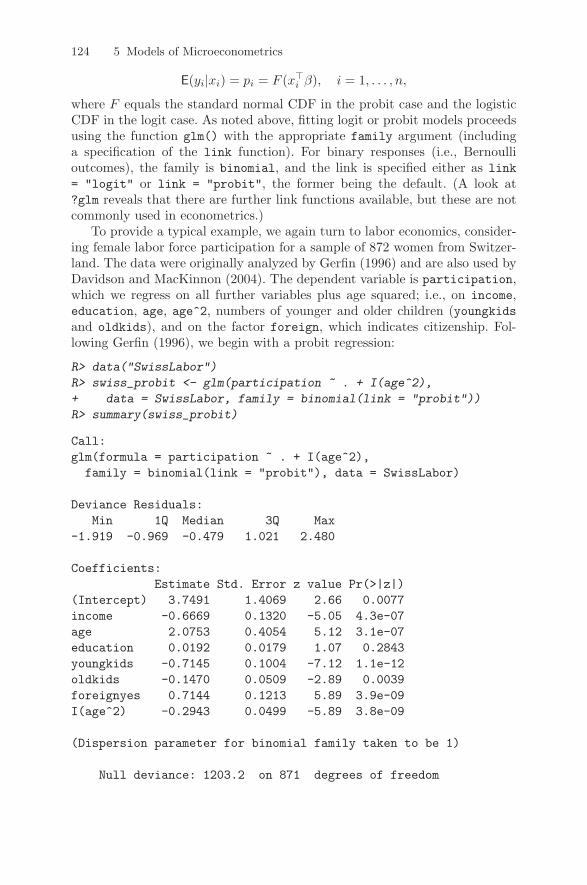
124 5 Models of Microeconometrics

E(yi|xi) = pi = F (x>i β), i = 1, . . . , n,

where F equals the standard normal CDF in the probit case and the logisticCDF in the logit case. As noted above, fitting logit or probit models proceedsusing the function glm() with the appropriate family argument (includinga specification of the link function). For binary responses (i.e., Bernoullioutcomes), the family is binomial, and the link is specified either as link= "logit" or link = "probit", the former being the default. (A look at?glm reveals that there are further link functions available, but these are notcommonly used in econometrics.)

To provide a typical example, we again turn to labor economics, consider-ing female labor force participation for a sample of 872 women from Switzer-land. The data were originally analyzed by Gerfin (1996) and are also used byDavidson and MacKinnon (2004). The dependent variable is participation,which we regress on all further variables plus age squared; i.e., on income,education, age, age^2, numbers of younger and older children (youngkidsand oldkids), and on the factor foreign, which indicates citizenship. Fol-lowing Gerfin (1996), we begin with a probit regression:

R> data("SwissLabor")

R> swiss_probit <- glm(participation ~ . + I(age^2),

+ data = SwissLabor, family = binomial(link = "probit"))

R> summary(swiss_probit)

Call:glm(formula = participation ~ . + I(age^2),family = binomial(link = "probit"), data = SwissLabor)

Deviance Residuals:Min 1Q Median 3Q Max

-1.919 -0.969 -0.479 1.021 2.480

Coefficients:Estimate Std. Error z value Pr(>|z|)

(Intercept) 3.7491 1.4069 2.66 0.0077income -0.6669 0.1320 -5.05 4.3e-07age 2.0753 0.4054 5.12 3.1e-07education 0.0192 0.0179 1.07 0.2843youngkids -0.7145 0.1004 -7.12 1.1e-12oldkids -0.1470 0.0509 -2.89 0.0039foreignyes 0.7144 0.1213 5.89 3.9e-09I(age^2) -0.2943 0.0499 -5.89 3.8e-09

(Dispersion parameter for binomial family taken to be 1)

Null deviance: 1203.2 on 871 degrees of freedom

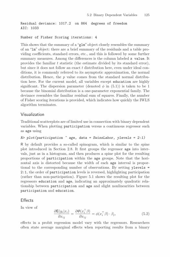
5.2 Binary Dependent Variables 125

Residual deviance: 1017.2 on 864 degrees of freedomAIC: 1033

Number of Fisher Scoring iterations: 4

This shows that the summary of a“glm”object closely resembles the summaryof an “lm” object: there are a brief summary of the residuals and a table pro-viding coefficients, standard errors, etc., and this is followed by some furthersummary measures. Among the differences is the column labeled z value. Itprovides the familiar t statistic (the estimate divided by its standard error),but since it does not follow an exact t distribution here, even under ideal con-ditions, it is commonly referred to its asymptotic approximation, the normaldistribution. Hence, the p value comes from the standard normal distribu-tion here. For the current model, all variables except education are highlysignificant. The dispersion parameter (denoted φ in (5.1)) is taken to be 1because the binomial distribution is a one-parameter exponential family. Thedeviance resembles the familiar residual sum of squares. Finally, the numberof Fisher scoring iterations is provided, which indicates how quickly the IWLSalgorithm terminates.

Visualization

Traditional scatterplots are of limited use in connection with binary dependentvariables. When plotting participation versus a continuous regressor suchas age using

R> plot(participation ~ age, data = SwissLabor, ylevels = 2:1)

R by default provides a so-called spinogram, which is similar to the spineplot introduced in Section 2.8. It first groups the regressor age into inter-vals, just as in a histogram, and then produces a spine plot for the resultingproportions of participation within the age groups. Note that the hori-zontal axis is distorted because the width of each age interval is propor-tional to the corresponding number of observations. By setting ylevels =2:1, the order of participation levels is reversed, highlighting participation(rather than non-participation). Figure 5.1 shows the resulting plot for theregressors education and age, indicating an approximately quadratic rela-tionship between participation and age and slight nonlinearities betweenparticipation and education.

Effects

In view of∂E(yi|xi)

∂xij=

∂Φ(x>i β)∂xij

= φ(x>i β) · βj , (5.2)

effects in a probit regression model vary with the regressors. Researchersoften state average marginal effects when reporting results from a binary

126 5 Models of Microeconometrics

Fig. 5.1. Spinograms for binary dependent variables.

GLM. There are several versions of such averages. It is perhaps best to usen−1

∑ni=1 φ(x>i β) · βj , the average of the sample marginal effects. In R, this is

simply

R> fav <- mean(dnorm(predict(swiss_probit, type = "link")))

R> fav * coef(swiss_probit)

(Intercept) income age education youngkids1.241930 -0.220932 0.687466 0.006359 -0.236682oldkids foreignyes I(age^2)

-0.048690 0.236644 -0.097505

Another version evaluates (5.2) at the average regressor, x. This is straight-forward as long as all regressors are continuous; however, more often thannot, the model includes factors. In this case, it is preferable to report averageeffects for all levels of the factors, averaging only over continuous regressors.In the case of the SwissLabor data, there is only a single factor, foreign, in-dicating whether the individual is Swiss or not. Thus, average marginal effectsfor these groups are available via

R> av <- colMeans(SwissLabor[, -c(1, 7)])

R> av <- data.frame(rbind(swiss = av, foreign = av),

+ foreign = factor(c("no", "yes")))

R> av <- predict(swiss_probit, newdata = av, type = "link")

R> av <- dnorm(av)

R> av["swiss"] * coef(swiss_probit)[-7]

(Intercept) income age education youngkids1.495137 -0.265976 0.827628 0.007655 -0.284938

education

part

icip

atio

n

0 6 8 10 12

yes

no

0.0

0.2

0.4

0.6

0.8

1.0

age

part

icip

atio

n

2 3 3.5 4 4.5 5 6

yes

no

0.0

0.2

0.4

0.6

0.8

1.0

5.2 Binary Dependent Variables 127

oldkids I(age^2)-0.058617 -0.117384

and

R> av["foreign"] * coef(swiss_probit)[-7]

(Intercept) income age education youngkids1.136517 -0.202180 0.629115 0.005819 -0.216593oldkids I(age^2)

-0.044557 -0.089229

This indicates that all effects are smaller in absolute size for the foreign women.Furthermore, methods for visualizing effects in linear and generalized linear

models are available in the package effects (Fox 2003).

Goodness of fit and prediction

In contrast to the linear regression model, there is no commonly acceptedversion of R2 for generalized linear models, not even for the special case ofbinary dependent variables.

R2 measures for nonlinear models are often called pseudo-R2s. If we define`(β) as the log-likelihood for the fitted model and `(y) as the log-likelihoodfor the model containing only a constant term, we can use a ratio of log-likelihoods,

R2 = 1− `(β)`(y)

,

often called McFadden’s pseudo-R2. This is easily made available in R bycomputing the null model, and then extracting the logLik() values for thetwo models

R> swiss_probit0 <- update(swiss_probit, formula = . ~ 1)

R> 1 - as.vector(logLik(swiss_probit)/logLik(swiss_probit0))

[1] 0.1546

yields a rather modest pseudo-R2 for the model fitted to the SwissLabor data.In the first line of the code chunk above, the update() call reevaluates theoriginal call using the formula corresponding to the null model. In the secondline, as.vector() strips off all additional attributes returned by logLik()(namely the "class" and "df" attributes).

A further way of assessing the fit of a binary regression model is to comparethe categories of the observed responses with their fitted values. This requiresprediction for GLMs. The generic function predict() also has a method forobjects of class “glm”. However, for GLMs, things are slightly more involvedthan for linear models in that there are several types of predictions. Specifi-cally, the predict() method for “glm” objects has a type argument allowing

128 5 Models of Microeconometrics

types "link", "response", and "terms". The default "link" is on the scaleof the linear predictors, and "response" is on the scale of the mean of theresponse variable. For a binary regression model, the default predictions arethus of probabilities on the logit or probit scales, while type = "response"yields the predicted probabilities themselves. (In addition, the "terms" optionreturns a matrix giving the fitted values of each term in the model formulaon the linear-predictor scale.)

In order to obtain the predicted class, we round the predicted probabili-ties and tabulate the result against the actual values of participation in aconfusion matrix,

R> table(true = SwissLabor$participation,

+ pred = round(fitted(swiss_probit)))

predtrue 0 1no 337 134yes 146 255

corresponding to 67.89% correctly classified and 32.11% misclassified obser-vations in the observed sample.

However, this evaluation of the model uses the arbitrarily chosen cutoff 0.5for the predicted probabilities. To avoid choosing a particular cutoff, the per-formance can be evaluated for every conceivable cutoff; e.g., using (as above)the“accuracy”of the model, the proportion of correctly classified observations,as the performance measure. The left panel of Figure 5.2 indicates that thebest accuracy is achieved for a cutoff slightly below 0.5.

Alternatively, the receiver operating characteristic (ROC) curve can beused: for every cutoff c ∈ [0, 1], the associated true positive rate (TPR(c),in our case the number of women participating in the labor force that arealso classified as participating compared with the total number of womenparticipating) is plotted against the false positive rate (FPR(c), in our casethe number of women not participating in the labor force that are classified asparticipating compared with the total number of women not participating).Thus, ROC = (FPR(c),TPR(c)) | c ∈ [0, 1], and this curve is displayed inthe right panel of Figure 5.2. For a sensible predictive model, the ROC curveshould be at least above the diagonal (which corresponds to random guessing).The closer the curve is to the upper left corner (FPR = 0, TPR = 1), thebetter the model performs.

In R, visualizations of these (and many other performance measures) can becreated using the ROCR package (Sing, Sander, Beerenwinkel, and Lengauer2005). In the first step, the observations and predictions are captured in anobject created by prediction(). Subsequently, various performances can becomputed and plotted:

R> library("ROCR")

R> pred <- prediction(fitted(swiss_probit),

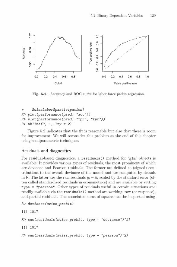
5.2 Binary Dependent Variables 129

Fig. 5.2. Accuracy and ROC curve for labor force probit regression.

+ SwissLabor$participation)

R> plot(performance(pred, "acc"))

R> plot(performance(pred, "tpr", "fpr"))

R> abline(0, 1, lty = 2)

Figure 5.2 indicates that the fit is reasonable but also that there is roomfor improvement. We will reconsider this problem at the end of this chapterusing semiparametric techniques.

Residuals and diagnostics

For residual-based diagnostics, a residuals() method for “glm” objects isavailable. It provides various types of residuals, the most prominent of whichare deviance and Pearson residuals. The former are defined as (signed) con-tributions to the overall deviance of the model and are computed by defaultin R. The latter are the raw residuals yi− µi scaled by the standard error (of-ten called standardized residuals in econometrics) and are available by settingtype = "pearson". Other types of residuals useful in certain situations andreadily available via the residuals() method are working, raw (or response),and partial residuals. The associated sums of squares can be inspected using

R> deviance(swiss_probit)

[1] 1017

R> sum(residuals(swiss_probit, type = "deviance")^2)

[1] 1017

R> sum(residuals(swiss_probit, type = "pearson")^2)

Cutoff

Acc

urac

y

0.0 0.2 0.4 0.6 0.8

0.50

0.60

0.70

False positive rate

Tru

e po

sitiv

e ra

te

0.0 0.2 0.4 0.6 0.8 1.0

0.0

0.2

0.4

0.6

0.8

1.0

130 5 Models of Microeconometrics

[1] 866.5

and an analysis of deviance is performed by the anova() method for “glm”ob-jects. Other standard tests for nested model comparisons, such as waldtest(),linear.hypothesis(), and coeftest(), are available as well.

We also note that sandwich estimates of the covariance matrix are availablein the usual manner, and thus

R> coeftest(swiss_probit, vcov = sandwich)

would give the usual regression output with robustified standard errors andt statistics. However, the binary case differs from the linear regression modelin that it is not possible to misspecify the variance while correctly specifyingthe regression equation. Instead, both are either correctly specified or not.Thus, users must be aware that, in the case where conventional and sandwichstandard errors are very different, there are likely to be problems with theregression itself and not just with the variances of the estimates. Therefore, wedo not recommend general use of sandwich estimates in the binary regressioncase (see also Freedman 2006, for further discussion). Sandwich estimates aremuch more useful and less controversial in Poisson regressions, as discussedin the following section.

(Quasi-)complete separation

To conclude this section, we briefly discuss an issue that occasionally ariseswith probit or logit regressions. For illustration, we consider a textbook ex-ample inspired by Stokes (2004). The goal is to study the deterrent effectof capital punishment in the United States of America in 1950 utilizing theMurderRates data taken from Maddala (2001). Maddala uses these data toillustrate probit and logit models, apparently without noticing that there is aproblem.

Running a logit regression of an indicator of the incidence of executions(executions) during 1946–1950 on the median time served of convicted mur-derers released in 1951 (time in months), the median family income in 1949(income), the labor force participation rate (in percent) in 1950 (lfp), theproportion of the population that was non-Caucasian in 1950 (noncauc), anda factor indicating region (southern) yields, using the defaults of the estima-tion process,

R> data("MurderRates")

R> murder_logit <- glm(I(executions > 0) ~ time + income +

+ noncauc + lfp + southern, data = MurderRates,

+ family = binomial)

Warning message:fitted probabilities numerically 0 or 1 occurred in:glm.fit(x = X, y = Y, weights = weights, start = start,

5.2 Binary Dependent Variables 131

Thus, calling glm() results in a warning message according to which somefitted probabilities are numerically identical to zero or one. Also, the standarderror of southern is suspiciously large:

R> coeftest(murder_logit)

z test of coefficients:

Estimate Std. Error z value Pr(>|z|)(Intercept) 10.9933 20.7734 0.53 0.597time 0.0194 0.0104 1.87 0.062income 10.6101 5.6541 1.88 0.061noncauc 70.9879 36.4118 1.95 0.051lfp -0.6676 0.4767 -1.40 0.161southernyes 17.3313 2872.1707 0.01 0.995

Clearly, this model deserves a closer look. The warning suggests that numericalproblems were encountered, so it is advisable to modify the default settingsof the IWLS algorithm in order to determine the source of the phenomenon.The relevant argument to glm() is control, which takes a list consisting ofthe entries epsilon, the convergence tolerance epsilon, maxit, the maximumnumber of IWLS iterations, and trace, the latter indicating if intermediateoutput is required for each iteration. Simultaneously decreasing the epsilonand increasing the maximum number of iterations yields

R> murder_logit2 <- glm(I(executions > 0) ~ time + income +

+ noncauc + lfp + southern, data = MurderRates,

+ family = binomial, control = list(epsilon = 1e-15,

+ maxit = 50, trace = FALSE))

Warning message:fitted probabilities numerically 0 or 1 occurred in:glm.fit(x = X, y = Y, weights = weights, start = start,

Interestingly, the warning does not go away and the coefficient on southernhas doubled, accompanied by a 6,000-fold increase of the corresponding stan-dard error:

R> coeftest(murder_logit2)

z test of coefficients:

Estimate Std. Error z value Pr(>|z|)(Intercept) 1.10e+01 2.08e+01 0.53 0.597time 1.94e-02 1.04e-02 1.87 0.062income 1.06e+01 5.65e+00 1.88 0.061noncauc 7.10e+01 3.64e+01 1.95 0.051lfp -6.68e-01 4.77e-01 -1.40 0.161southernyes 3.13e+01 1.73e+07 1.8e-06 1.000

132 5 Models of Microeconometrics

The explanation of this phenomenon is somewhat technical: although the like-lihood of the logit model is known to be globally concave and bounded fromabove, this does not imply that an interior maximum exists. This is preciselythe problem we encountered here, and it depends on the settings of the func-tion call when and where the algorithm terminates. Termination does notmean that a maximum was found, just that it was not possible to increasethe objective function beyond the tolerance epsilon supplied. Specifically, wehave here a situation where the maximum likelihood estimator does not exist.Instead, there exists a β0 such that

yi = 0 whenever x>i β0 ≤ 0,

yi = 1 whenever x>i β0 ≥ 0.

If this is the case, the data are said to exhibit quasi-complete separation(the case of strict inequalities being called complete separation). Althoughthe effect is not uncommon with small data sets, it is rarely discussed intextbooks; Davidson and MacKinnon (2004) is an exception.

For the problem at hand, the change in the coefficient on southern alreadyindicates that this variable alone is responsible for the effect. A tabulationreveals

R> table(I(MurderRates$executions > 0), MurderRates$southern)

no yesFALSE 9 0TRUE 20 15

In short, all of the 15 southern states, plus 20 of the remaining ones, executedconvicted murderers during the period in question; thus the variable southernalone contains a lot of information on the dependent variable.

In practical terms, complete or quasi-complete separation is not necessarilya nuisance. After all, we are able to perfectly distinguish the zeros from theones. However, many practitioners find it counterintuitive, if not disturbing,that the nonexistence of the MLE might be beneficial in some situations. Notealso that inspection of the individual t statistics in coeftest(murder_logit)suggests excluding southern. As a result, the warning would have gone away,but the predictions would have been worse. The message is to carefully studysuch warnings in regressions with a binary dependent variable, with hugestandard errors often pointing to the source of the problem.

5.3 Regression Models for Count Data

In this section, we consider a number of regression models for count data.A convenient reference on the methodological background is Cameron andTrivedi (1998). For illustration, we use the RecreationDemand data previ-ously analyzed by Ozuna and Gomez (1995) and Gurmu and Trivedi (1996),

5.3 Regression Models for Count Data 133

among others. The data are cross-section data on the number of recreationalboating trips to Lake Somerville, Texas, in 1980, based on a survey adminis-tered to 2,000 registered leisure boat owners in 23 counties in eastern Texas.The dependent variable is trips, and we want to regress it on all furthervariables: a (subjective) quality ranking of the facility (quality), a factorindicating whether the individual engaged in water-skiing at the lake (ski),household income (income), a factor indicating whether the individual paida user’s fee at the lake (userfee), and three cost variables (costC, costS,costH) representing opportunity costs.

We begin with the standard model for count data, a Poisson regression.As noted above, this is a generalized linear model. Using the canonical linkfor the Poisson family (the log link), the model is

E(yi|xi) = µi = exp(x>i β).

Fitting is as simple as

R> data("RecreationDemand")

R> rd_pois <- glm(trips ~ ., data = RecreationDemand,

+ family = poisson)

To save space, we only present the partial coefficient tests and not the fullsummary() output:

R> coeftest(rd_pois)

z test of coefficients:

Estimate Std. Error z value Pr(>|z|)(Intercept) 0.26499 0.09372 2.83 0.0047quality 0.47173 0.01709 27.60 < 2e-16skiyes 0.41821 0.05719 7.31 2.6e-13income -0.11132 0.01959 -5.68 1.3e-08userfeeyes 0.89817 0.07899 11.37 < 2e-16costC -0.00343 0.00312 -1.10 0.2713costS -0.04254 0.00167 -25.47 < 2e-16costH 0.03613 0.00271 13.34 < 2e-16

This would seem to indicate that almost all regressors are highly significant.For later reference, we note the log-likelihood of the fitted model:

R> logLik(rd_pois)

'log Lik.' -1529 (df=8)

Dealing with overdispersion

Recall that the Poisson distribution has the property that the variance equalsthe mean (“equidispersion”). This built-in feature needs to be checked in any

134 5 Models of Microeconometrics

empirical application. In econometrics, Poisson regressions are often plaguedby overdispersion, meaning that the variance is larger than the linear predictorpermits.

One way of testing for overdispersion is to consider the alternative hypoth-esis (Cameron and Trivedi 1990)

Var(yi|xi) = µi + α · h(µi), (5.3)

where h is a positive function of µi. Overdispersion corresponds to α > 0and underdispersion to α < 0. The coefficient α can be estimated by anauxiliary OLS regression and tested with the corresponding t statistic, whichis asymptotically standard normal under the null hypothesis of equidispersion.

Common specifications of the transformation function h are h(µ) = µ2 orh(µ) = µ. The former corresponds to a negative binomial (NB) model (seebelow) with quadratic variance function (called NB2 by Cameron and Trivedi1998), the latter to an NB model with linear variance function (called NB1by Cameron and Trivedi 1998). In the statistical literature, the reparameter-ization

Var(yi|xi) = (1 + α) · µi = dispersion · µi (5.4)

of the NB1 model is often called a quasi-Poisson model with dispersion pa-rameter.

The package AER provides the function dispersiontest() for testingequidispersion against alternative (5.3). By default, the parameterization (5.4)is used. Alternatively, if the argument trafo is specified, the test is formulatedin terms of the parameter α. Tests against the quasi-Poisson formulation andthe NB2 alternative are therefore available using

R> dispersiontest(rd_pois)

Overdispersion test

data: rd_poisz = 2.412, p-value = 0.007941alternative hypothesis: true dispersion is greater than 1sample estimates:dispersion

6.566

and

R> dispersiontest(rd_pois, trafo = 2)

Overdispersion test

data: rd_poisz = 2.938, p-value = 0.001651alternative hypothesis: true alpha is greater than 0

5.3 Regression Models for Count Data 135

sample estimates:alpha1.316

Both suggest that the Poisson model for the trips data is not well specified inthat there appears to be a substantial amount of overdispersion.

One possible remedy is to consider a more flexible distribution that doesnot impose equality of mean and variance. The most widely used distribu-tion in this context is the negative binomial. It may be considered a mixturedistribution arising from a Poisson distribution with random scale, the latterfollowing a gamma distribution. Its probability mass function is

f(y;µ, θ) =Γ (θ + y)Γ (θ)y!

µyθθ

(µ + θ)y+θ, y = 0, 1, 2, . . . , µ > 0, θ > 0.

The variance of the negative binomial distribution is given by

Var(y;µ, θ) = µ +1θµ2,

which is of the form (5.3) with h(µ) = µ2 and α = 1/θ.If θ is known, this distribution is of the general form (5.1). The Poisson

distribution with parameter µ arises for θ → ∞. The geometric distributionis the special case where θ = 1.

In R, tools for negative binomial regression are provided by the MASSpackage (Venables and Ripley 2002). Specifically, for estimating negative bi-nomial GLMs with known θ, the function negative.binomial() can be used;e.g., for a geometric regression via family = negative.binomial(theta =1). For unknown θ, the function glm.nb() is available. Thus

R> library("MASS")

R> rd_nb <- glm.nb(trips ~ ., data = RecreationDemand)

R> coeftest(rd_nb)

z test of coefficients:

Estimate Std. Error z value Pr(>|z|)(Intercept) -1.12194 0.21430 -5.24 1.6e-07quality 0.72200 0.04012 18.00 < 2e-16skiyes 0.61214 0.15030 4.07 4.6e-05income -0.02606 0.04245 -0.61 0.539userfeeyes 0.66917 0.35302 1.90 0.058costC 0.04801 0.00918 5.23 1.7e-07costS -0.09269 0.00665 -13.93 < 2e-16costH 0.03884 0.00775 5.01 5.4e-07

136 5 Models of Microeconometrics

R> logLik(rd_nb)

'log Lik.' -825.6 (df=9)

provides a new model for the trips data. The shape parameter of the fitted neg-ative binomial distribution is θ = 0.7293, suggesting a considerable amount ofoverdispersion and confirming the results from the test for overdispersion. Wenote that the negative binomial model represents a substantial improvementin terms of likelihood.

Robust standard errors

Instead of switching to a more general family of distributions, it is also possibleto use the Poisson estimates along with a set of standard errors estimatedunder less restrictive assumptions, provided the mean is correctly specified.The package sandwich implements sandwich variance estimators for GLMsvia the sandwich() function. In microeconometric applications, the resultingestimates are often called Huber-White standard errors. For the problem athand, Poisson and Huber-White errors are rather different:

R> round(sqrt(rbind(diag(vcov(rd_pois)),

+ diag(sandwich(rd_pois)))), digits = 3)

(Intercept) quality skiyes income userfeeyes costC costS[1,] 0.094 0.017 0.057 0.02 0.079 0.003 0.002[2,] 0.432 0.049 0.194 0.05 0.247 0.015 0.012

costH[1,] 0.003[2,] 0.009

This again indicates that the simple Poisson model is inadequate. Regressionoutput utilizing robust standard errors is available using

R> coeftest(rd_pois, vcov = sandwich)

z test of coefficients:

Estimate Std. Error z value Pr(>|z|)(Intercept) 0.26499 0.43248 0.61 0.54006quality 0.47173 0.04885 9.66 < 2e-16skiyes 0.41821 0.19387 2.16 0.03099income -0.11132 0.05031 -2.21 0.02691userfeeyes 0.89817 0.24691 3.64 0.00028costC -0.00343 0.01470 -0.23 0.81549costS -0.04254 0.01173 -3.62 0.00029costH 0.03613 0.00939 3.85 0.00012

It should be noted that the sandwich estimator is based on first and secondderivatives of the likelihood: the outer product of gradients (OPG) forms the

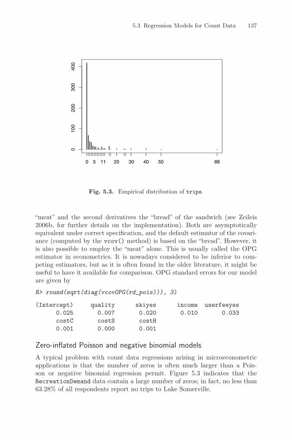
5.3 Regression Models for Count Data 137

Fig. 5.3. Empirical distribution of trips.

“meat” and the second derivatives the “bread” of the sandwich (see Zeileis2006b, for further details on the implementation). Both are asymptoticallyequivalent under correct specification, and the default estimator of the covari-ance (computed by the vcov() method) is based on the “bread”. However, itis also possible to employ the “meat” alone. This is usually called the OPGestimator in econometrics. It is nowadays considered to be inferior to com-peting estimators, but as it is often found in the older literature, it might beuseful to have it available for comparison. OPG standard errors for our modelare given by

R> round(sqrt(diag(vcovOPG(rd_pois))), 3)

(Intercept) quality skiyes income userfeeyes0.025 0.007 0.020 0.010 0.033costC costS costH0.001 0.000 0.001

Zero-inflated Poisson and negative binomial models

A typical problem with count data regressions arising in microeconometricapplications is that the number of zeros is often much larger than a Pois-son or negative binomial regression permit. Figure 5.3 indicates that theRecreationDemand data contain a large number of zeros; in fact, no less than63.28% of all respondents report no trips to Lake Somerville.

010

020

030

040

0

0 5 11 20 30 40 50 88

138 5 Models of Microeconometrics

However, the Poisson regression fitted above only provides 41.96% of zeroobservations, again suggesting that this model is not satisfactory. A closerlook at observed and expected counts reveals

R> rbind(obs = table(RecreationDemand$trips)[1:10], exp = round(

+ sapply(0:9, function(x) sum(dpois(x, fitted(rd_pois))))))

0 1 2 3 4 5 6 7 8 9obs 417 68 38 34 17 13 11 2 8 1exp 277 146 68 41 30 23 17 13 10 7

This again underlines that there are problems with the previously consideredspecification. In fact, the variance-to-mean ratio for the trips variable equals17.64, a value usually too large to be accommodated by covariates. Alternativemodels are needed.

One such model is the zero-inflated Poisson (ZIP) model (Lambert 1992),which suggests a mixture specification with a Poisson count component andan additional point mass at zero. With IA(y) denoting the indicator function,the basic idea is

fzeroinfl(y) = pi · I0(y) + (1− pi) · fcount(y;µi),

where now µi and pi are modeled as functions of the available covariates. Em-ploying the canonical link for the count part gives log(µi) = x>i β, while for thebinary part g(pi) = z>i γ for some quantile function g, with the canonical linkgiven by the logistic distribution and the probit link as a popular alternative.Note that the two sets of regressors xi and zi need not be identical.

The package pscl provides a function zeroinfl() for fitting this familyof models (Zeileis, Kleiber, and Jackman 2008), allowing Poisson, geometric,and negative binomial distributions for the count component fcount(y).

Following Cameron and Trivedi (1998), we consider a regression of tripson all further variables for the count part (using a negative binomial distribu-tion) and model the inflation part as a function of quality and income:

R> rd_zinb <- zeroinfl(trips ~ . | quality + income,

+ data = RecreationDemand, dist = "negbin")

This specifies the linear predictor in the count part as employing all avail-able regressors, while the inflation part, separated by |, only uses qualityand income. The inflation part by default uses the logit model, but all otherlinks available in glm() may also be used upon setting the argument linkappropriately. For the RecreationDemand data, a ZINB model yields

R> summary(rd_zinb)

Call:zeroinfl(formula = trips ~ . | quality + income,data = RecreationDemand, dist = "negbin")

5.3 Regression Models for Count Data 139

Count model coefficients (negbin with log link):Estimate Std. Error z value Pr(>|z|)

(Intercept) 1.09663 0.25668 4.27 1.9e-05quality 0.16891 0.05303 3.19 0.00145skiyes 0.50069 0.13449 3.72 0.00020income -0.06927 0.04380 -1.58 0.11378userfeeyes 0.54279 0.28280 1.92 0.05494costC 0.04044 0.01452 2.79 0.00534costS -0.06621 0.00775 -8.55 < 2e-16costH 0.02060 0.01023 2.01 0.04415Log(theta) 0.19017 0.11299 1.68 0.09235

Zero-inflation model coefficients (binomial with logit link):Estimate Std. Error z value Pr(>|z|)

(Intercept) 5.743 1.556 3.69 0.00022quality -8.307 3.682 -2.26 0.02404income -0.258 0.282 -0.92 0.35950

Theta = 1.209Number of iterations in BFGS optimization: 26Log-likelihood: -722 on 12 Df

showing a clearly improved log-likelihood compared with the plain negativebinomial model. The expected counts are given by

R> round(colSums(predict(rd_zinb, type = "prob")[,1:10]))

0 1 2 3 4 5 6 7 8 9433 47 35 27 20 16 12 10 8 7

which shows that both the zeros and the remaining counts are captured muchbetter than in the previous models. Note that the predict() method for type= "prob" returns a matrix that provides a vector of expected probabilitiesfor each observation. By taking column sums, the expected counts can becomputed, here for 0, . . . , 9.

Hurdle models

Another model that is able to capture excessively large (or small) numbers ofzeros is the hurdle model (Mullahy 1986). In economics, it is more widely usedthan the zero-inflation model presented above. The hurdle model consists oftwo parts (hence it is also called a “two-part model”):

• A binary part (given by a count distribution right-censored at y = 1):Is yi equal to zero or positive? “Is the hurdle crossed?”

• A count part (given by a count distribution left-truncated at y = 1):If yi > 0, how large is yi?

140 5 Models of Microeconometrics

This results in a model with

fhurdle(y;x, z, β, γ)

=

fzero(0; z, γ), if y = 0,1− fzero(0; z, γ) · fcount(y;x, β)/1− fcount(0;x, β), if y > 0.

The hurdle model is somewhat easier to fit than the zero-inflation modelbecause the resulting likelihood decomposes into two parts that may be max-imized separately.

The package pscl also provides a function hurdle(). Again followingCameron and Trivedi (1998), we consider a regression of trips on all fur-ther variables for the count part and model the inflation part as a function ofonly quality and income. The available distributions in hurdle() are againPoisson, negative binomial, and geometric.

We warn readers that there exist several parameterizations of hurdle mod-els that differ with respect to the hurdle mechanism. Here it is possible tospecify either a count distribution right-censored at one or a Bernoulli distri-bution distinguishing between zeros and non-zeros (which is equivalent to theright-censored geometric distribution). The first variant appears to be morecommon in econometrics; however, the Bernoulli specification is more intu-itively interpretable as a hurdle (and hence used by default in hurdle()).Here, we employ the latter, which is equivalent to the geometric distributionused by Cameron and Trivedi (1998).

R> rd_hurdle <- hurdle(trips ~ . | quality + income,

+ data = RecreationDemand, dist = "negbin")

R> summary(rd_hurdle)

Call:hurdle(formula = trips ~ . | quality + income,data = RecreationDemand, dist = "negbin")

Count model coefficients (truncated negbin with log link):Estimate Std. Error z value Pr(>|z|)

(Intercept) 0.8419 0.3828 2.20 0.0278quality 0.1717 0.0723 2.37 0.0176skiyes 0.6224 0.1901 3.27 0.0011income -0.0571 0.0645 -0.88 0.3763userfeeyes 0.5763 0.3851 1.50 0.1345costC 0.0571 0.0217 2.63 0.0085costS -0.0775 0.0115 -6.71 1.9e-11costH 0.0124 0.0149 0.83 0.4064Log(theta) -0.5303 0.2611 -2.03 0.0423

5.4 Censored Dependent Variables 141

Zero hurdle model coefficients (binomial with logit link):Estimate Std. Error z value Pr(>|z|)

(Intercept) -2.7663 0.3623 -7.64 2.3e-14quality 1.5029 0.1003 14.98 < 2e-16income -0.0447 0.0785 -0.57 0.57

Theta: count = 0.588Number of iterations in BFGS optimization: 18Log-likelihood: -765 on 12 Df

Again, we consider the expected counts:

R> round(colSums(predict(rd_hurdle, type = "prob")[,1:10]))

0 1 2 3 4 5 6 7 8 9417 74 42 27 19 14 10 8 6 5

Like the ZINB model, the negative binomial hurdle model results in a consid-erable improvement over the initial Poisson specification.

Further details on fitting, assessing and comparing regression models forcount data can be found in Zeileis et al. (2008).

5.4 Censored Dependent Variables

Censored dependent variables have been used in econometrics ever since To-bin (1958) modeled the demand for durable goods by means of a censoredlatent variable. Specifically, the tobit model posits a Gaussian linear modelfor a latent variable, say y0. y0 is only observed if positive; otherwise zero isreported:

y0i = x>i β + εi, εi|xi ∼ N (0, σ2) i.i.d.,

yi =

y0i , y0

i > 0,0, y0

i ≤ 0.

The log-likelihood of this model is thus given by

`(β, σ2) =∑yi>0

(log φ(yi − x>i β)/σ − log σ

)+

∑yi=0

log Φ(x>i β/σ).

To statisticians, especially biostatisticians, this is a special case of a censoredregression model. An R package for fitting such models has long been available,which is the survival package accompanying Therneau and Grambsch (2000).(In fact, survival even contains Tobin’s original data; readers may want toexplore data("tobin") there.) However, many aspects of that package willnot look familiar to econometricians, and thus our package AER comes witha convenience function tobit() interfacing survival’s survreg() function.

142 5 Models of Microeconometrics

We illustrate the mechanics using a famous—or perhaps infamous—dataset taken from Fair (1978). It is available as Affairs in AER and providesthe results of a survey on extramarital affairs conducted by the US magazinePsychology Today in 1969. The dependent variable is affairs, the number ofextramarital affairs during the past year, and the available regressors includeage, yearsmarried, children (a factor indicating the presence of children),occupation (a numeric score coding occupation), and rating (a numericvariable coding the self-rating of the marriage; the scale is 1 through 5, with5 indicating “very happy”).

We note that the dependent variable is a count and is thus perhaps bestanalyzed along different lines; however, for historical reasons and for com-parison with sources such as Greene (2003), we follow the classical approach.(Readers are asked to explore count data models in an exercise.)

tobit() has a formula interface like lm(). For the classical tobit modelwith left-censoring at zero, only this formula and a data set are required:

R> data("Affairs")

R> aff_tob <- tobit(affairs ~ age + yearsmarried +

+ religiousness + occupation + rating, data = Affairs)

R> summary(aff_tob)

Call:tobit(formula = affairs ~ age + yearsmarried +religiousness + occupation + rating, data = Affairs)

Observations:Total Left-censored Uncensored Right-censored601 451 150 0

Coefficients:Estimate Std. Error z value Pr(>|z|)

(Intercept) 8.1742 2.7414 2.98 0.0029age -0.1793 0.0791 -2.27 0.0234yearsmarried 0.5541 0.1345 4.12 3.8e-05religiousness -1.6862 0.4038 -4.18 3.0e-05occupation 0.3261 0.2544 1.28 0.2000rating -2.2850 0.4078 -5.60 2.1e-08Log(scale) 2.1099 0.0671 31.44 < 2e-16

Scale: 8.25

Gaussian distributionNumber of Newton-Raphson Iterations: 4Log-likelihood: -706 on 7 DfWald-statistic: 67.7 on 5 Df, p-value: 3.1e-13

5.4 Censored Dependent Variables 143

The output comprises the usual regression output along with the value of thelog-likelihood and a Wald statistic paralleling the familiar regression F statis-tic. For convenience, a tabulation of censored and uncensored observations isalso included. The results indicate that yearsmarried and rating are themain “risk factors”.

To further illustrate the arguments to tobit(), we refit the model byintroducing additional censoring from the right:

R> aff_tob2 <- update(aff_tob, right = 4)

R> summary(aff_tob2)

Call:tobit(formula = affairs ~ age + yearsmarried +religiousness + occupation + rating, right = 4,data = Affairs)

Observations:Total Left-censored Uncensored Right-censored601 451 70 80

Coefficients:Estimate Std. Error z value Pr(>|z|)

(Intercept) 7.9010 2.8039 2.82 0.00483age -0.1776 0.0799 -2.22 0.02624yearsmarried 0.5323 0.1412 3.77 0.00016religiousness -1.6163 0.4244 -3.81 0.00014occupation 0.3242 0.2539 1.28 0.20162rating -2.2070 0.4498 -4.91 9.3e-07Log(scale) 2.0723 0.1104 18.77 < 2e-16

Scale: 7.94

Gaussian distributionNumber of Newton-Raphson Iterations: 4Log-likelihood: -500 on 7 DfWald-statistic: 42.6 on 5 Df, p-value: 4.5e-08

The standard errors are now somewhat larger, reflecting the fact that heav-ier censoring leads to a loss of information. tobit() also permits, via theargument dist, alternative distributions of the latent variable, including thelogistic and Weibull distributions.

Among the methods for objects of class “tobit”, we briefly consider aWald-type test:

R> linear.hypothesis(aff_tob, c("age = 0", "occupation = 0"),

+ vcov = sandwich)

144 5 Models of Microeconometrics

Linear hypothesis test

Hypothesis:age = 0occupation = 0

Model 1: affairs ~ age + yearsmarried + religiousness +occupation + rating

Model 2: restricted model

Note: Coefficient covariance matrix supplied.

Res.Df Df Chisq Pr(>Chisq)1 5942 596 -2 4.91 0.086

Thus, the regressors age and occupation are jointly weakly significant. Forillustration, we use a sandwich covariance estimate, although it should beborne in mind that, as in the binary and unlike the Poisson case, in thismodel, misspecification of the variance typically also means misspecificationof the mean (see again Freedman 2006, for further discussion).

5.5 Extensions

The number of models used in microeconometrics has grown considerably overthe last two decades. Due to space constraints, we can only afford to brieflydiscuss a small selection. We consider a semiparametric version of the binaryresponse model as well as multinomial and ordered logit models.

Table 5.2 provides a list of further relevant packages.

A semiparametric binary response model

Recall that the log-likelihood of the binary response model is

`(β) =n∑

i=1

yi log F (x>i β) + (1− yi) log1− F (x>i β)

,

where F is the CDF of the logistic or the Gaussian distribution in the logit orprobit case, respectively. The Klein and Spady (1993) approach estimates Fvia kernel methods, and thus it may be considered a semiparametric maximumlikelihood estimator. In another terminology, it is a semiparametric single-index model. We refer to Li and Racine (2007) for a recent exposition.

In R, the Klein and Spady estimator is available in the package np (Hayfieldand Racine 2008), the package accompanying Li and Racine (2007). Sincethe required functions from that package currently do not accept factors asdependent variables, we preprocess the SwissLabor data via

5.5 Extensions 145

Table 5.2. Further packages for microeconometrics.

Package Description

gam Generalized additive models (Hastie 2006)

lme4 Nonlinear random-effects models: counts, binary depen-dent variables, etc. (Bates 2008)

mgcv Generalized additive (mixed) models (Wood 2006)

micEcon Demand systems, cost and production functions (Hen-ningsen 2008)

mlogit Multinomial logit models with choice-specific variables(Croissant 2008)

robustbase Robust/resistant regression for GLMs (Maechler,Rousseeuw, Croux, Todorov, Ruckstuhl, and Salibian-Barrera 2007)

sampleSelection Selection models: generalized tobit, heckit (Toomet andHenningsen 2008)

R> SwissLabor$partnum <- as.numeric(SwissLabor$participation) - 1

which creates a dummy variable partnum within SwissLabor that codes non-participation and participation as 0 and 1, respectively. Fitting itself requiresfirst computing a bandwidth object using the function npindexbw(), as in

R> library("np")

R> swiss_bw <- npindexbw(partnum ~ income + age + education +

+ youngkids + oldkids + foreign + I(age^2), data = SwissLabor,

+ method = "kleinspady", nmulti = 5)

A summary of the bandwidths is available via

R> summary(swiss_bw)

Single Index ModelRegression data (872 observations, 7 variable(s)):

income age education youngkids oldkids foreignBeta: 1 -2.219 -0.0249 -5.515 0.1797 -0.8268

I(age^2)Beta: 0.3427Bandwidth: 0.383Optimisation Method: Nelder-MeadRegression Type: Local-ConstantBandwidth Selection Method: Klein and Spady

146 5 Models of Microeconometrics

Formula: partnum ~ income + age + education + youngkids +oldkids + foreign + I(age^2)

Objective Function Value: 0.5934 (achieved on multistart 3)

Continuous Kernel Type: Second-Order GaussianNo. Continuous Explanatory Vars.: 1

Finally, the Klein and Spady estimate is given by passing the bandwidth objectswiss_bw to npindex():

R> swiss_ks <- npindex(bws = swiss_bw, gradients = TRUE)

R> summary(swiss_ks)

Single Index ModelRegression Data: 872 training points, in 7 variable(s)

income age education youngkids oldkids foreignBeta: 1 -2.219 -0.0249 -5.515 0.1797 -0.8268

I(age^2)Beta: 0.3427Bandwidth: 0.383Kernel Regression Estimator: Local-Constant

Confusion MatrixPredicted

Actual 0 10 345 1261 137 264

Overall Correct Classification Ratio: 0.6984Correct Classification Ratio By Outcome:

0 10.7325 0.6584

McFadden-Puig-Kerschner performance measure fromprediction-realization tables: 0.6528

Continuous Kernel Type: Second-Order GaussianNo. Continuous Explanatory Vars.: 1

The resulting confusion matrix may be compared with the confusion matrixof the original probit model (see Section 5.2),

R> table(Actual = SwissLabor$participation, Predicted =

+ round(predict(swiss_probit, type = "response")))

5.5 Extensions 147

PredictedActual 0 1

no 337 134yes 146 255

showing that the semiparametric model has slightly better (in-sample) per-formance.

When applying semiparametric procedures such as the Klein and Spadymethod, one should be aware that these are rather time-consuming (despitethe optimized and compiled C code underlying the np package). In fact, themodel above takes more time than all other examples together when compilingthis book on the authors’ machines.

Multinomial responses

For illustrating the most basic version of the multinomial logit model, a modelwith only individual-specific covariates, we consider the BankWages data takenfrom Heij, de Boer, Franses, Kloek, and van Dijk (2004). It contains, for em-ployees of a US bank, an ordered factor job with levels "custodial", "admin"(for administration), and "manage" (for management), to be modeled as afunction of education (in years) and a factor minority indicating minoritystatus. There also exists a factor gender, but since there are no women in thecategory "custodial", only a subset of the data corresponding to males isused for parametric modeling below.

To obtain a first overview of how job depends on education, a table ofconditional proportions can be generated via

R> data("BankWages")

R> edcat <- factor(BankWages$education)

R> levels(edcat)[3:10] <- rep(c("14-15", "16-18", "19-21"),

+ c(2, 3, 3))

R> tab <- xtabs(~ edcat + job, data = BankWages)

R> prop.table(tab, 1)

jobedcat custodial admin manage8 0.245283 0.754717 0.00000012 0.068421 0.926316 0.00526314-15 0.008197 0.959016 0.03278716-18 0.000000 0.367089 0.63291119-21 0.000000 0.033333 0.966667

where education has been transformed into a categorical variable with someof the sparser levels merged. This table can also be visualized in a spine plotvia

R> plot(job ~ edcat, data = BankWages, off = 0)

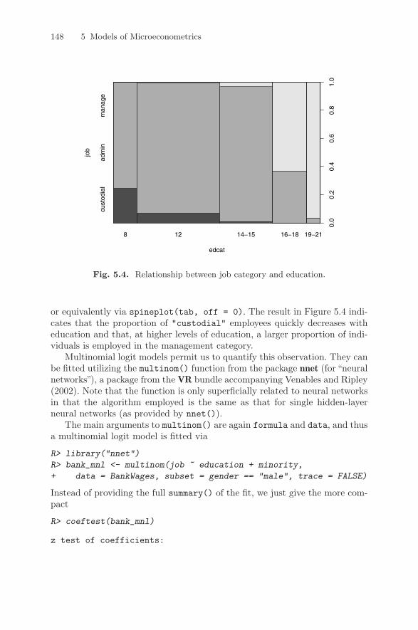
148 5 Models of Microeconometrics

Fig. 5.4. Relationship between job category and education.

or equivalently via spineplot(tab, off = 0). The result in Figure 5.4 indi-cates that the proportion of "custodial" employees quickly decreases witheducation and that, at higher levels of education, a larger proportion of indi-viduals is employed in the management category.

Multinomial logit models permit us to quantify this observation. They canbe fitted utilizing the multinom() function from the package nnet (for “neuralnetworks”), a package from the VR bundle accompanying Venables and Ripley(2002). Note that the function is only superficially related to neural networksin that the algorithm employed is the same as that for single hidden-layerneural networks (as provided by nnet()).

The main arguments to multinom() are again formula and data, and thusa multinomial logit model is fitted via

R> library("nnet")

R> bank_mnl <- multinom(job ~ education + minority,

+ data = BankWages, subset = gender == "male", trace = FALSE)

Instead of providing the full summary() of the fit, we just give the more com-pact

R> coeftest(bank_mnl)

z test of coefficients:

edcat

job

8 12 14−15 16−18 19−21

cust

odia

lad

min

man

age

0.0

0.2

0.4

0.6

0.8

1.0

5.5 Extensions 149

Estimate Std. Error z value Pr(>|z|)admin:(Intercept) -4.761 1.173 -4.06 4.9e-05admin:education 0.553 0.099 5.59 2.3e-08admin:minorityyes -0.427 0.503 -0.85 0.3957manage:(Intercept) -30.775 4.479 -6.87 6.4e-12manage:education 2.187 0.295 7.42 1.2e-13manage:minorityyes -2.536 0.934 -2.71 0.0066

This confirms that the proportions of "admin" and "manage" job categories(as compared with the reference category, here "custodial") increase witheducation and decrease for minority. Both effects seem to be stronger forthe "manage" category.

We add that, in contrast to multinom(), the recent package mlogit (Crois-sant 2008) also fits multinomial logit models containing “choice-specific” (i.e.,outcome-specific) attributes.

Ordinal responses

The dependent variable job in the preceding example can be considered anordered response, with "custodial" < "admin" < "manage". This suggeststhat an ordered logit or probit regression may be worth exploring; here weconsider the former. In the statistical literature, this is often called propor-tional odds logistic regression; hence the name polr() for the fitting functionfrom the MASS package (which, despite its name, can also fit ordered probitmodels upon setting method="probit"). Here, this yields

R> library("MASS")

R> bank_polr <- polr(job ~ education + minority,

+ data = BankWages, subset = gender == "male", Hess = TRUE)

R> coeftest(bank_polr)

z test of coefficients:

Estimate Std. Error z value Pr(>|z|)education 0.8700 0.0931 9.35 < 2e-16minorityyes -1.0564 0.4120 -2.56 0.010custodial|admin 7.9514 1.0769 7.38 1.5e-13admin|manage 14.1721 0.0941 150.65 < 2e-16

using again the more concise output of coeftest() rather than summary().The ordered logit model just estimates different intercepts for the different jobcategories but a common set of regression coefficients. The results are similarto those for the multinomial model, but the different education and minorityeffects for the different job categories are, of course, lost. This appears todeteriorate the model fit as the AIC increases:

R> AIC(bank_mnl)

150 5 Models of Microeconometrics

[1] 249.5

R> AIC(bank_polr)

[1] 268.6

5.6 Exercises

1. For the SwissLabor data, plotting participation versus education (seeFigure 5.1) suggests a nonlinear effect of education. Fit a model utilizingeducation squared in addition to the regressors considered in Section 5.2.Does the new model result in an improvement?

2. The PSID1976 data originating from Mroz (1987) are used in many econo-metrics texts, including Greene (2003) and Wooldridge (2002). FollowingGreene (2003, p. 681):(a) Fit a probit model for labor force participation using the regressors

age, age squared, family income, education, and a factor indicatingthe presence of children. (The factor needs to be constructed from theavailable information.)

(b) Reestimate the model assuming that different equations apply towomen with and without children.

(c) Perform a likelihood ratio test to check whether the more generalmodel is really needed.

3. Analyze the DoctorVisits data, taken from Cameron and Trivedi (1998),using a Poisson regression for the number of visits. Is the Possion modelsatisfactory? If not, where are the problems and what could be done aboutthem?

4. As mentioned above, the Affairs data are perhaps better analyzed uti-lizing models for count data rather than a tobit model as we did here.Explore a Poisson regression and some of its variants, and be sure tocheck whether the models accommodate the many zeros present in thesedata.

5. Using the PSID1976 data, run a tobit regression of hours worked on non-wife income (to be constructed from the available information), age, ex-perience, experience squared, education, and the numbers of younger andolder children.

6

Time Series

Time series arise in many fields of economics, especially in macroeconomicsand financial economics. Here, we denote a time series (univariate or multi-variate) as yt, t = 1, . . . , n. This chapter first provides a brief overview ofR’s time series classes and “naive” methods such as the classical decomposi-tion into a trend, a seasonal component, and a remainder term, as well asexponential smoothing and related techniques. It then moves on to autore-gressive moving average (ARMA) models and extensions. We discuss classicalBox-Jenkins style analysis based on the autocorrelation and partial autocor-relation functions (ACF and PACF) as well as model selection via informationcriteria.

Many time series in economics are nonstationary. Nonstationarity oftencomes in one of two forms: the time series can be reduced to stationarity bydifferencing or detrending, or it contains structural breaks and is thereforeonly piecewise stationary. The third section therefore shows how to performthe standard unit-root and stationarity tests as well as cointegration tests.The fourth section discusses the analysis of structural change, where R offersa particularly rich set of tools for testing as well as dating breaks. The finalsection briefly discusses structural time series models and volatility models.

Due to space constraints, we confine ourselves to time domain methods.However, all the standard tools for analysis in the frequency domain, notablyestimates of the spectral density by several techniques, are available as well.In fact, some of these methods have already been used, albeit implicitly, inconnection with HAC covariance estimation in Chapter 4.

6.1 Infrastructure and “Naive” Methods

Classes for time series data

In the previous chapters, we already worked with different data structuresthat can hold rectangular data matrices, most notably “data.frame” for

C. Kleiber, A. Zeileis, Applied Econometrics with R,DOI: 10.1007/978-0-387-77318-6 6, © Springer Science+Business Media, LLC 2008

152 6 Time Series

cross-sectional data. Dealing with time series data poses slightly different chal-lenges. While we also need a rectangular, typically numeric, data matrix, inaddition, some way of storing the associated time points of the series is re-quired. R offers several classes for holding such data. Here, we discuss the twomost important (closely related) classes, “ts” and “zoo”.

R ships with the basic class “ts” for representing time series data; it isaimed at regular series, in particular at annual, quarterly, and monthly data.Objects of class “ts” are either a numeric vector (for univariate series) ora numeric matrix (for multivariate series) containing the data, along with a"tsp" attribute reflecting the time series properties. This is a vector of lengththree containing the start and end times (in time units) and the frequency.Time series objects of class “ts” can easily be created with the function ts()by supplying the data (a numeric vector or matrix), along with the argumentsstart, end, and frequency. Methods for standard generic functions such asplot(), lines(), str(), and summary() are provided as well as various time-series-specific methods, such as lag() or diff(). As an example, we loadand plot the univariate time series UKNonDurables, containing the quarterlyconsumption of non-durables in the United Kingdom (taken from Franses1998).

R> data("UKNonDurables")

R> plot(UKNonDurables)

The resulting time series plot is shown in the left panel of Figure 6.1. Thetime series properties

R> tsp(UKNonDurables)

[1] 1955.00 1988.75 4.00

reveal that this is a quarterly series starting in 1955(1) and ending in 1988(4).If the series of all time points is needed, it can be extracted via time(); e.g.,time(UKNonDurables). Subsets can be chosen using the function window();e.g.,

R> window(UKNonDurables, end = c(1956, 4))

Qtr1 Qtr2 Qtr3 Qtr41955 24030 25620 26209 271671956 24620 25972 26285 27659

Single observations can be extracted by setting start and end to the samevalue.

The “ts” class is well suited for annual, quarterly, and monthly time se-ries. However, it has two drawbacks that make it difficult to use in someapplications: (1) it can only deal with numeric time stamps (and not withmore general date/time classes); (2) internal missing values cannot be omit-ted (because then the start/end/frequency triple is no longer sufficient for

6.1 Infrastructure and “Naive” Methods 153

Fig. 6.1. Quarterly time series of consumption of non-durables in the UnitedKingdom (left) and monthly number of car drivers killed or seriously injured in theUnited Kingdom (right, with filtered version).

reconstructing all time stamps). Both are major nuisances when working withirregular series (e.g., with many financial time series). Consequently, vari-ous implementations for irregular time series have emerged in contributed Rpackages, the most flexible of which is “zoo”, provided by the zoo1 package(Zeileis and Grothendieck 2005). It can have time stamps of arbitrary typeand is designed to be as similar as possible to “ts”. Specifically, the series areessentially also numeric vectors or matrices but with an "index" attributecontaining the full vector of indexes (or time stamps) rather than only the"tsp" attribute with start/end/frequency. Therefore, “zoo” series can be seenas a generalization of“ts”series. Most methods that work for“ts”objects alsowork for “zoo” objects, some have extended functionality, and some new onesare provided. Regular series can be coerced back and forth between the classeswithout loss of information using the functions as.zoo() and as.ts(). Hence,it does not make much difference which of these two classes is used for annual,quarterly, or monthly data—whereas “zoo” is much more convenient for dailydata (e.g., coupled with an index of class “Date”) or intraday data (e.g., with“POSIXct” or “chron” time stamps). See Zeileis and Grothendieck (2005) forfurther details on “zoo” series and Grothendieck and Petzoldt (2004) for moreon date/time classes in R.

Throughout this book, we mainly rely on the “ts” class; only in very fewillustrations where additional flexibility is required do we switch to “zoo”.1 zoo stands for Z’s ordered observations, named after the author who started the

development of the package.

Time

UK

Non

Dur

able

s

1955 1965 1975 1985

3000

050

000

Time

UK

Driv

erD

eath

s

1970 1975 1980 1985

1000

1500

2000

2500

154 6 Time Series

(Linear) filtering

One of the most basic tools for transforming time series (e.g., for eliminatingseasonality) is linear filtering (see Brockwell and Davis 1991, 1996). An im-portant class of linear filters are finite moving averages, transformations thatreplace the raw data yt by a weighted sum

yt =s∑

j=−r

ajyt+j , t = r + 1, . . . , n− s.

If r equals s, the filter is called symmetric. In R, the function filter() permitsthe use of fairly general filters; its argument filter takes a vector containingthe coefficients aj . Apart from moving averages (default, see above), filter()can also apply recursive linear filters, another important class of filters.

As an example, we consider the monthly time series UKDriverDeaths con-taining the well-known data from Harvey and Durbin (1986) on car driverskilled or seriously injured in the United Kingdom from 1969(1) through1984(12). These are also known as the “seatbelt data”, as they were usedby Harvey and Durbin (1986) for evaluating the effectiveness of compulsorywearing of seatbelts introduced on 1983-01-31. The following code loads andplots the series along with a filtered version utilizing the simple symmetricmoving average of length 13 with coefficients (1/24, 1/12, . . . , 1/12, 1/24)>.

R> data("UKDriverDeaths")

R> plot(UKDriverDeaths)

R> lines(filter(UKDriverDeaths, c(1/2, rep(1, 11), 1/2)/12),

+ col = 2)

The resulting plot is depicted in the right panel of Figure 6.1, illustrating thatthe filter eliminates seasonality. Other classical filters, such as the Hendersonor Spencer filters (Brockwell and Davis 1991), can be applied analogously.

Another function that can be used for evaluating linear and nonlinearfunctions on moving data windows is rollapply() (for rolling apply). Thiscan be used for computing running means via rollapply(UKDriverDeaths,12, mean), yielding a result similar to that for the symmetric filter above, orrunning standard deviations

R> plot(rollapply(UKDriverDeaths, 12, sd))

shown in the right panel of Figure 6.2, revealing increased variation aroundthe time of the policy intervention.

As mentioned above, filter() also provides autoregressive (recursive)filtering. This can be exploited for simple simulations; e.g., from AR(1) models.The code

R> set.seed(1234)

R> x <- filter(rnorm(100), 0.9, method = "recursive")

6.1 Infrastructure and “Naive” Methods 155

Fig. 6.2. UK driver deaths: trends from two season-trend decompositions (left)and running standard deviations (right).

generates 100 observations from an AR(1) process with parameter 0.9 andstandard normal innovations. A more elaborate tool for simulating from gen-eral ARIMA models is provided by arima.sim().

Decomposition

Filtering with moving averages can also be used for an additive or multi-plicative decomposition into seasonal, trend, and irregular components. Theclassical approach to this task, implemented in the function decompose(), isto take a simple symmetric filter as illustrated above for extracting the trendand derive the seasonal component by averaging the trend-adjusted observa-tions from corresponding periods. A more sophisticated approach that alsoaccommodates time-varying seasonal components is seasonal decompositionvia loess smoothing (Cleveland, Cleveland, McRae, and Terpenning 1990). Itis available in the function stl() and iteratively finds the seasonal and trendcomponents by loess smoothing of the observations in moving data windowsof a certain size. Both methods are easily applied in R using (in keeping withthe original publication, we employ logarithms)

R> dd_dec <- decompose(log(UKDriverDeaths))

R> dd_stl <- stl(log(UKDriverDeaths), s.window = 13)

where the resulting objects dd_dec and dd_stl hold the trend, seasonal, andirregular components in slightly different formats (a list for the“decomposed.ts” and a multivariate time series for the “stl” object). Bothclasses have plotting methods drawing time series plots of the componentswith a common time axis. The result of plot(dd_stl) is provided inFigure 6.3, and the result of plot(dd_dec) looks rather similar. (The bars

Time

tren

d

1970 1975 1980 1985

7.2

7.3

7.4

7.5

7.6

Time

rolla

pply

(UK

Driv

erD

eath

s, 1

2, s

d)

1970 1975 1980 1985

150

200

250

300

350

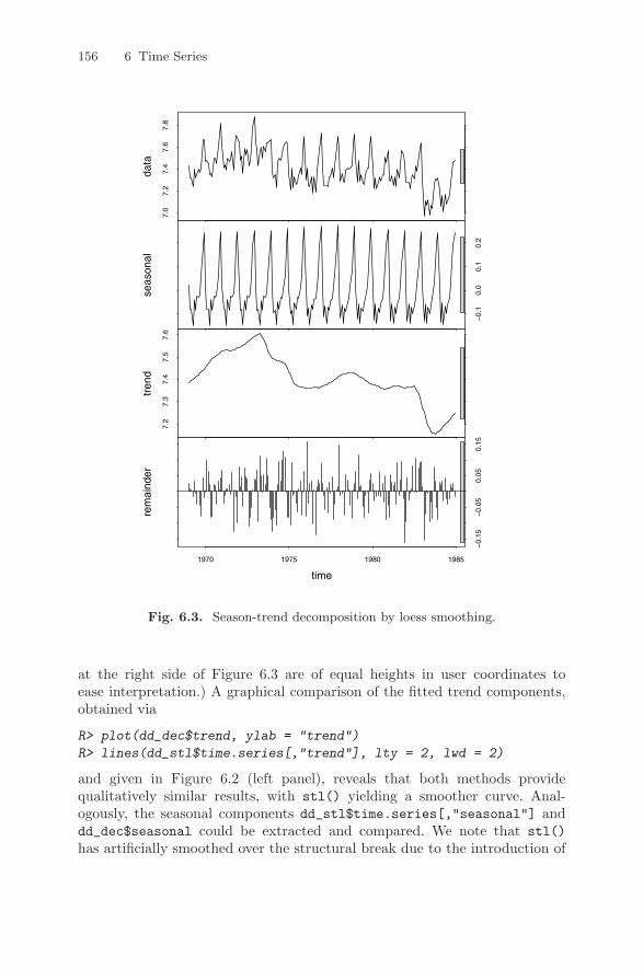
156 6 Time Series

Fig. 6.3. Season-trend decomposition by loess smoothing.

at the right side of Figure 6.3 are of equal heights in user coordinates toease interpretation.) A graphical comparison of the fitted trend components,obtained via

R> plot(dd_dec$trend, ylab = "trend")

R> lines(dd_stl$time.series[,"trend"], lty = 2, lwd = 2)

and given in Figure 6.2 (left panel), reveals that both methods providequalitatively similar results, with stl() yielding a smoother curve. Anal-ogously, the seasonal components dd_stl$time.series[,"seasonal"] anddd_dec$seasonal could be extracted and compared. We note that stl()has artificially smoothed over the structural break due to the introduction of

7.0

7.2

7.4

7.6

7.8

data

−0.

10.

00.

10.

2

seas

onal

7.2

7.3

7.4

7.5

7.6

tren

d

−0.

15−

0.05

0.05

0.15

1970 1975 1980 1985

rem

aind

er

time

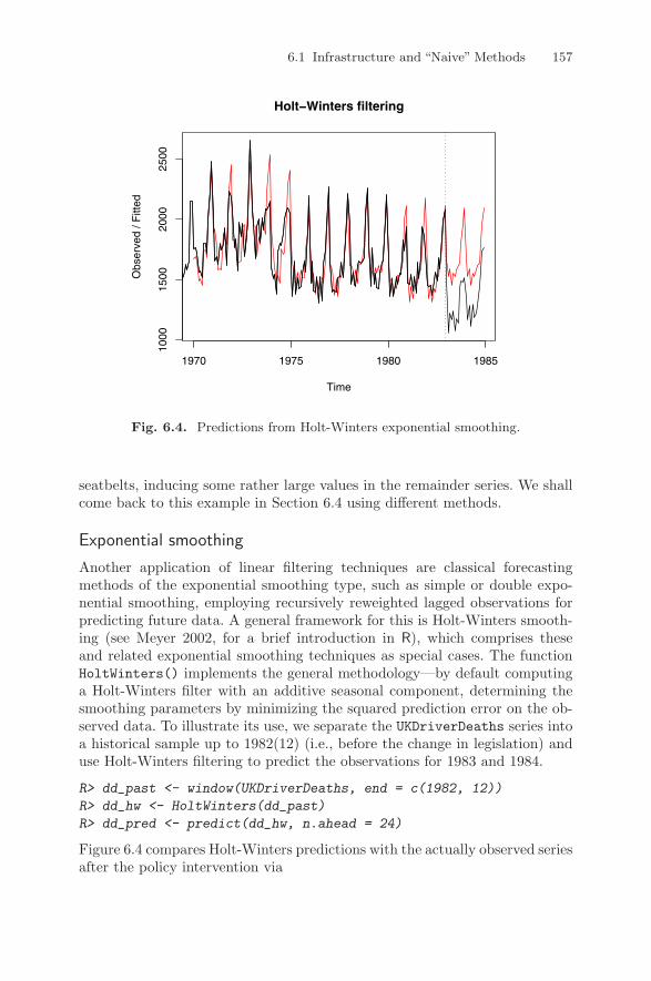
6.1 Infrastructure and “Naive” Methods 157

Fig. 6.4. Predictions from Holt-Winters exponential smoothing.

seatbelts, inducing some rather large values in the remainder series. We shallcome back to this example in Section 6.4 using different methods.

Exponential smoothing

Another application of linear filtering techniques are classical forecastingmethods of the exponential smoothing type, such as simple or double expo-nential smoothing, employing recursively reweighted lagged observations forpredicting future data. A general framework for this is Holt-Winters smooth-ing (see Meyer 2002, for a brief introduction in R), which comprises theseand related exponential smoothing techniques as special cases. The functionHoltWinters() implements the general methodology—by default computinga Holt-Winters filter with an additive seasonal component, determining thesmoothing parameters by minimizing the squared prediction error on the ob-served data. To illustrate its use, we separate the UKDriverDeaths series intoa historical sample up to 1982(12) (i.e., before the change in legislation) anduse Holt-Winters filtering to predict the observations for 1983 and 1984.

R> dd_past <- window(UKDriverDeaths, end = c(1982, 12))

R> dd_hw <- HoltWinters(dd_past)

R> dd_pred <- predict(dd_hw, n.ahead = 24)

Figure 6.4 compares Holt-Winters predictions with the actually observed seriesafter the policy intervention via

Holt−Winters filtering

Time

Obs

erve

d / F

itted

1970 1975 1980 1985

1000

1500

2000

2500

158 6 Time Series

R> plot(dd_hw, dd_pred, ylim = range(UKDriverDeaths))

R> lines(UKDriverDeaths)

showing that the number of road casualties clearly dropped after the intro-duction of mandatory wearing of seatbelts.

We conclude by noting that a more sophisticated function for exponen-tial smoothing algorithms, named ets(), is available in the package forecast(Hyndman and Khandakar 2008).

6.2 Classical Model-Based Analysis

The classical approach to parametric modeling and forecasting is to employan autoregressive integrated moving average (ARIMA) model for capturingthe dependence structure in a time series (Brockwell and Davis 1991; Box andJenkins 1970; Hamilton 1994). To fix the notation, ARIMA(p, d, q) models aredefined by the equation

φ(L)(1− L)dyt = θ(L)εt, (6.1)

where the autoregressive (AR) part is given by the pth-order polynomialφ(L) = 1− φ1L− . . .− φpL

p in the lag operator L, the moving average (MA)part is given by the qth-order polynomial θ(L) = 1+θ1L+ . . .+θqL

q, and d isthe order of differencing. (Note the sign convention for the MA polynomial.)

For ease of reference, Table 6.1 provides a partial list of time series fittingfunctions (with StructTS() being discussed in Section 6.5).

Fig. 6.5. (Partial) autocorrelation function.

0 5 10 15 20

−0.

20.

20.

61.

0

Lag

AC

F

Series x

5 10 15 20

−0.

20.

20.

61.

0

Lag

Par

tial A

CF

Series x

6.2 Classical Model-Based Analysis 159

Table 6.1. Time series fitting functions in R.

Function Package Description

ar() stats Fits univariate autoregressions via Yule-Walker, OLS,ML, or Burg’s method and unrestricted VARs by Yule-Walker, OLS, or Burg’s method. Order selection by AICpossible.

arima() stats Fits univariate ARIMA models, including seasonal(SARIMA) models, models with covariates (ARIMAX),and subset ARIMA models, by unconditional ML or byCSS.

arma() tseries Fits ARMA models by CSS. Starting values via Hannan-Rissanen. Note: Parameterization of intercept differentfrom arima().

auto.arima() forecast Order selection via AIC, BIC, or AICC within a user-defined set of models. Fitting is done via arima().

StructTS() stats Fits structural time series models: local level, local trend,and basic structural model.

Before fitting an ARIMA model to a series, it is helpful to first take anexploratory look at the empirical ACF and PACF. In R, these are available inthe functions acf() and pacf(), respectively. For the artificial AR(1) processx from the previous section, they are computed and plotted by

R> acf(x)

R> pacf(x)

and shown in Figure 6.5. Here, the maximum number of lags defaults to10 log10(n), but it can be changed by the argument lag.max. Plotting canbe suppressed by setting plot = FALSE. This is useful when the (P)ACF isneeded for further computations.

The empirical ACF for series x decays only slowly, while the PACF ex-ceeds the individual confidence limits only for lag 1, reflecting clearly how theseries was generated. Next we try to recover the true structure by fitting anautoregression to x via the function ar():

R> ar(x)

Call:ar(x = x)

Coefficients:1

0.928

160 6 Time Series

Order selected 1 sigma^2 estimated as 1.29

This agrees rather well with the true autocorrelation of 0.9. By default, ar()fits AR models up to lag p = 10 log10(n) and selects the minimum AIC model.This is usually a good starting point for model selection, even though the de-fault estimator is the Yule-Walker estimator, which is considered a preliminaryestimator. ML is also available in addition to OLS and Burg estimation; see?ar for further details.

For a real-world example, we return to the UKNonDurables series, aimingat establishing a model for the (log-transformed) observations up to 1970(4)for predicting the remaining series.

R> nd <- window(log(UKNonDurables), end = c(1970, 4))

The corresponding time series plot (see Figure 6.1) suggests rather clearlythat differencing is appropriate; hence the first row of Figure 6.6 depicts theempirical ACF and PACF of the differenced series. As both exhibit a strongseasonal pattern (already visible in the original series), the second row ofFigure 6.6 also shows the empirical ACF and PACF after double differencing(at the seasonal lag 4 and at lag 1) as generated by

R> acf(diff(nd), ylim = c(-1, 1))

R> pacf(diff(nd), ylim = c(-1, 1))

R> acf(diff(diff(nd, 4)), ylim = c(-1, 1))

R> pacf(diff(diff(nd, 4)), ylim = c(-1, 1))

For this series, a model more general than a simple AR model is needed:arima() fits general ARIMA models, including seasonal ARIMA (SARIMA)models and models containing further regressors (utilizing the argumentxreg), either via ML or minimization of the conditional sum of squares (CSS).The default is to use CSS to obtain starting values and then ML for refine-ment. As the model space is much more complex than in the AR(p) case,where only the order p has to be chosen, base R does not offer an automaticmodel selection method for general ARIMA models based on information cri-teria. Therefore, we use the preliminary results from the exploratory analy-sis above and R’s general tools to set up a model search for an appropriateSARIMA(p, d, q)(P,D,Q)4 model,

Φ(L4)φ(L)(1− L4)D(1− L)dyt = θ(L)Θ(L4)εt, (6.2)

which amends the standard ARIMA model (6.1) by additional polynomialsoperating on the seasonal frequency.

The graphical analysis clearly suggests double differencing of the originalseries (d = 1, D = 1), some AR and MA effects (we allow p = 0, 1, 2 andq = 0, 1, 2), and low-order seasonal AR and MA parts (we use P = 0, 1 andQ = 0, 1), giving a total of 36 parameter combinations to consider. Of course,higher values for p, q, P , and Q could also be assessed. We refrain from doing so

6.2 Classical Model-Based Analysis 161

Fig. 6.6. (Partial) autocorrelation functions for UK non-durables data.

to save computation time in this example—however, we encourage readers topursue this issue for higher-order models as well. We also note that the packageforecast (Hyndman and Khandakar 2008) contains a function auto.arima()that performs a search over a user-defined set of models, just as we do heremanually. To choose from the 36 possible models, we set up all parametercombinations via expand.grid(), fit each of the associated SARIMA modelsusing arima() in a for() loop, and store the resulting BIC extracted fromthe model (obtained via AIC() upon setting k = log(length(nd))).

R> nd_pars <- expand.grid(ar = 0:2, diff = 1, ma = 0:2,

+ sar = 0:1, sdiff = 1, sma = 0:1)

R> nd_aic <- rep(0, nrow(nd_pars))

R> for(i in seq(along = nd_aic)) nd_aic[i] <- AIC(arima(nd,

0 1 2 3 4

−1.

0−

0.5

0.0

0.5

1.0

Lag

AC

F

Series diff(nd)

1 2 3 4

−1.

0−

0.5

0.0

0.5

1.0

Lag

Par

tial A

CF

Series diff(nd)

0 1 2 3 4

−1.

0−

0.5

0.0

0.5

1.0

Lag

AC

F

Series diff(diff(nd, 4))

1 2 3 4

−1.

0−

0.5

0.0

0.5

1.0

Lag

Par

tial A

CF

Series diff(diff(nd, 4))

162 6 Time Series

+ unlist(nd_pars[i, 1:3]), unlist(nd_pars[i, 4:6])),

+ k = log(length(nd)))

R> nd_pars[which.min(nd_aic),]

ar diff ma sar sdiff sma22 0 1 1 0 1 1

These computations reveal that a SARIMA(0, 1, 1)(0, 1, 1)4 model is best interms of BIC, conforming well with the exploratory analysis. This model isalso famously known as the airline model due to its application to a series ofairline passengers in the classical text by Box and Jenkins (1970). It is refittedto nd via

R> nd_arima <- arima(nd, order = c(0,1,1), seasonal = c(0,1,1))

R> nd_arima

Call:arima(x = nd, order = c(0, 1, 1), seasonal = c(0, 1, 1))

Coefficients:ma1 sma1

-0.353 -0.583s.e. 0.143 0.138

sigma^2 estimated as 9.65e-05: log likelihood = 188.14,aic = -370.27

showing that both moving average coefficients are negative and significant. Toassess whether this model appropriately captures the dependence structure ofthe series, tsdiag() produces several diagnostic plots

R> tsdiag(nd_arima)

shown in Figure 6.7. In the first panel, the standardized residuals are plotted.They do not exhibit any obvious pattern. Their empirical ACF in the secondpanel shows no (individually) significant autocorrelation at lags > 1. Finally,the p values for the Ljung-Box statistic in the third panel all clearly exceed5% for all orders, indicating that there is no significant departure from whitenoise for the residuals.

As there are no obvious deficiencies in our model, it is now used for pre-dicting the remaining 18 years in the sample:

R> nd_pred <- predict(nd_arima, n.ahead = 18 * 4)

The object nd_pred contains the predictions along with their associated stan-dard errors and can be compared graphically with the observed series via

R> plot(log(UKNonDurables))

R> lines(nd_pred$pred, col = 2)

6.2 Classical Model-Based Analysis 163

Fig. 6.7. Diagnostics for SARIMA(0, 1, 1)(0, 1, 1)4 model.

Figure 6.8 shows that the general trend is captured reasonably well. However,the model systematically overpredicts for certain parts of the sample in the1980s.

We conclude by adding that there exist, apart from generic functions suchas coef(), logLik(), predict(), print(), and vcov(), which also work onobjects of class “Arima” (the class of objects returned by arima()), severalfurther convenience functions for exploring ARMA models and their repre-sentations. These are listed in Table 6.2.

Standardized Residuals

Time

1955 1960 1965 1970

−3

−2

−1

01

2

0 1 2 3 4

−0.

20.

20.

61.

0

Lag

AC

F

ACF of Residuals

2 4 6 8 10

0.0

0.2

0.4

0.6

0.8

1.0

p values for Ljung−Box statistic

lag

p va

lue

164 6 Time Series

Fig. 6.8. Predictions from SARIMA(0, 1, 1)(0, 1, 1)4 model.

Table 6.2. Convenience functions for ARMA models.

Function Package Description

acf2AR() stats Computes an AR process exactly fitting a given autocor-relation function.

arima.sim() stats Simulation of ARIMA models.

ARMAacf() stats Computes theoretical (P)ACF for a given ARMA model.

ARMAtoMA() stats Computes MA(∞) representation for a given ARMAmodel.

6.3 Stationarity, Unit Roots, and Cointegration

Many time series in macroeconomics and finance are nonstationary, the pre-cise form of the nonstationarity having caused a hot debate some 25 yearsago. Nelson and Plosser (1982) argued that macroeconomic time series oftenare more appropriately described by unit-root nonstationarity than by de-terministic time trends. We refer to Hamilton (1994) for an overview of themethodology. The Nelson and Plosser data (or rather an extended versionending in 1988) are available in R in the package tseries (Trapletti 2008), andwe shall use them for an exercise at the end of this chapter.

Time

log(

UK

Non

Dur

able

s)

1955 1960 1965 1970 1975 1980 1985 1990

10.2

10.4

10.6

10.8

11.0

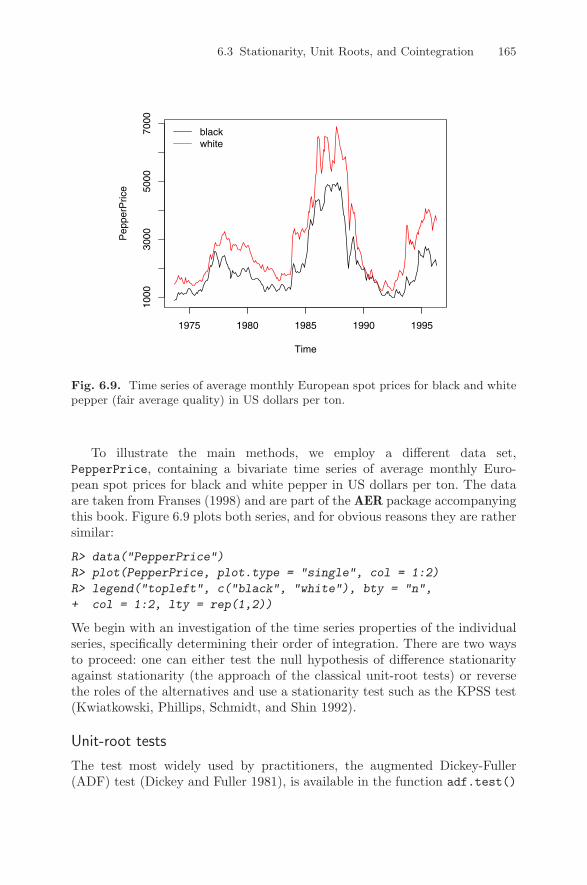
6.3 Stationarity, Unit Roots, and Cointegration 165

Fig. 6.9. Time series of average monthly European spot prices for black and whitepepper (fair average quality) in US dollars per ton.

To illustrate the main methods, we employ a different data set,PepperPrice, containing a bivariate time series of average monthly Euro-pean spot prices for black and white pepper in US dollars per ton. The dataare taken from Franses (1998) and are part of the AER package accompanyingthis book. Figure 6.9 plots both series, and for obvious reasons they are rathersimilar:

R> data("PepperPrice")

R> plot(PepperPrice, plot.type = "single", col = 1:2)

R> legend("topleft", c("black", "white"), bty = "n",

+ col = 1:2, lty = rep(1,2))

We begin with an investigation of the time series properties of the individualseries, specifically determining their order of integration. There are two waysto proceed: one can either test the null hypothesis of difference stationarityagainst stationarity (the approach of the classical unit-root tests) or reversethe roles of the alternatives and use a stationarity test such as the KPSS test(Kwiatkowski, Phillips, Schmidt, and Shin 1992).

Unit-root tests

The test most widely used by practitioners, the augmented Dickey-Fuller(ADF) test (Dickey and Fuller 1981), is available in the function adf.test()

Time

Pep

perP

rice

1975 1980 1985 1990 1995

1000

3000

5000

7000

blackwhite

166 6 Time Series

from the package tseries (Trapletti 2008). This function implements the t testof H0 : % = 0 in the regression

∆yt = α + δt + %yt−1 +k∑

j=1

φj∆yt−j + εt. (6.3)

The number of lags k defaults to b(n−1)1/3c but may be changed by the user.For the series corresponding to the price of white pepper, the test yields

R> library("tseries")

R> adf.test(log(PepperPrice[, "white"]))

Augmented Dickey-Fuller Test

data: log(PepperPrice[, "white"])Dickey-Fuller = -1.744, Lag order = 6, p-value = 0.6838alternative hypothesis: stationary

while, for the series of first differences, we obtain

R> adf.test(diff(log(PepperPrice[, "white"])))

Augmented Dickey-Fuller Test

data: diff(log(PepperPrice[, "white"]))Dickey-Fuller = -5.336, Lag order = 6, p-value = 0.01alternative hypothesis: stationary

Warning message:In adf.test(diff(log(PepperPrice[, "white"]))) :p-value smaller than printed p-value

Note that a warning is issued because the p value is only interpolated froma few tabulated critical values, and hence no p values outside the interval[0.01, 0.1] can be provided.

Alternatively, the Phillips-Perron test (Phillips and Perron 1988) with itsnonparametric correction for autocorrelation (essentially employing a HACestimate of the long-run variance in a Dickey-Fuller-type test (6.3) insteadof parametric decorrelation) can be used. It is available in the functionpp.test() from the package tseries (there also exists a function PP.test()in base R, but it has fewer options). Using the default options to the Phillips-Perron t test in the equation with a time trend, we obtain

R> pp.test(log(PepperPrice[, "white"]), type = "Z(t_alpha)")

Phillips-Perron Unit Root Test

data: log(PepperPrice[, "white"])

6.3 Stationarity, Unit Roots, and Cointegration 167

Dickey-Fuller Z(t_alpha) = -1.6439, Truncation lagparameter = 5, p-value = 0.726alternative hypothesis: stationary

Thus, all tests suggest that the null hypothesis of a unit root cannot be rejectedhere. Alternative implementations of the preceding methods with somewhatdifferent interfaces are available in the package urca (Pfaff 2006). That packagealso offers a function ur.ers() implementing the test of Elliott, Rothenberg,and Stock (1996), which utilizes GLS detrending.

Stationarity tests

Kwiatkowski et al. (1992) proceed by testing for the presence of a randomwalk component rt in the regression

yt = dt + rt + εt,

where dt denotes a deterministic component and εt is a stationary—moreprecisely, I(0)—error process. This test is also available in the functionkpss.test() in the package tseries. The deterministic component is eithera constant or a linear time trend, the former being the default. Setting theargument null = "Trend" yields the second version. Here, we obtain

R> kpss.test(log(PepperPrice[, "white"]))

KPSS Test for Level Stationarity

data: log(PepperPrice[, "white"])KPSS Level = 0.9129, Truncation lag parameter = 3,p-value = 0.01

Hence the KPSS test also points to nonstationarity of the pepper price series.(Again, a warning is issued, as the p value is interpolated from the four criticalvalues provided by Kwiatkowski et al. 1992, it is suppressed here.)

Readers may want to check that the series pertaining to black pepperyields similar results when tested for unit roots or stationarity.

Cointegration

The very nature of the two pepper series already suggests that they possesscommon features. Having evidence for nonstationarity, it is of interest to testfor a common nonstationary component by means of a cointegration test.

A simple method to test for cointegration is the two-step method proposedby Engle and Granger (1987). It regresses one series on the other and performsa unit root test on the residuals. This test, often named after Phillips andOuliaris (1990), who provided the asymptotic theory, is available in the func-tion po.test() from the package tseries. Specifically, po.test() performs a

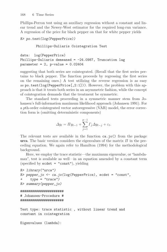
168 6 Time Series

Phillips-Perron test using an auxiliary regression without a constant and lin-ear trend and the Newey-West estimator for the required long-run variance.A regression of the price for black pepper on that for white pepper yields

R> po.test(log(PepperPrice))

Phillips-Ouliaris Cointegration Test

data: log(PepperPrice)Phillips-Ouliaris demeaned = -24.0987, Truncation lagparameter = 2, p-value = 0.02404

suggesting that both series are cointegrated. (Recall that the first series per-tains to black pepper. The function proceeds by regressing the first serieson the remaining ones.) A test utilizing the reverse regression is as easyas po.test(log(PepperPrice[,2:1])). However, the problem with this ap-proach is that it treats both series in an asymmetric fashion, while the conceptof cointegration demands that the treatment be symmetric.

The standard tests proceeding in a symmetric manner stem from Jo-hansen’s full-information maximum likelihood approach (Johansen 1991). Fora pth-order cointegrated vector autoregressive (VAR) model, the error correc-tion form is (omitting deterministic components)

∆yt = Πyt−1 +p−1∑j=1

Γj∆yt−j + εt.

The relevant tests are available in the function ca.jo() from the packageurca. The basic version considers the eigenvalues of the matrix Π in the pre-ceding equation. We again refer to Hamilton (1994) for the methodologicalbackground.

Here, we employ the trace statistic—the maximum eigenvalue, or“lambda-max”, test is available as well—in an equation amended by a constant term(specified by ecdet = "const"), yielding

R> library("urca")

R> pepper_jo <- ca.jo(log(PepperPrice), ecdet = "const",

+ type = "trace")

R> summary(pepper_jo)

####################### Johansen-Procedure #######################

Test type: trace statistic , without linear trend andconstant in cointegration

Eigenvalues (lambda):

6.4 Time Series Regression and Structural Change 169

[1] 4.93195e-02 1.35081e-02 1.38778e-17

Values of teststatistic and critical values of test:

test 10pct 5pct 1pctr <= 1 | 3.66 7.52 9.24 12.97r = 0 | 17.26 17.85 19.96 24.60

Eigenvectors, normalised to first column:(These are the cointegration relations)

black.l2 white.l2 constantblack.l2 1.000000 1.00000 1.00000white.l2 -0.889231 -5.09942 2.28091constant -0.556994 33.02742 -20.03244

Weights W:(This is the loading matrix)

black.l2 white.l2 constantblack.d -0.0747230 0.00245321 3.86752e-17white.d 0.0201561 0.00353701 4.03196e-18

The null hypothesis of no cointegration is rejected; hence the Johansen testconfirms the results from the initial two-step approach.

6.4 Time Series Regression and Structural Change

More on fitting dynamic regression models

As already discussed in Chapter 3, there are various ways of fitting dynamiclinear regression models by OLS in R. Here, we present two approaches inmore detail: (1) setting up lagged and differenced regressors “by hand” andcalling lm(); (2) using the convenience interface dynlm() from the packagedynlm (Zeileis 2008). We illustrate both approaches using a model for theUKDriverDeaths series: the log-casualties are regressed on their lags 1 and12, essentially corresponding to the multiplicative SARIMA(1, 0, 0)(1, 0, 0)12model

yt = β1 + β2 yt−1 + β3 yt−12 + εt, t = 13, . . . , 192.

For using lm() directly, we set up a multivariate time series containing theoriginal log-casualties along with two further variables holding the lagged ob-servations. The lagged variables are created with lag(). Note that its secondargument, the number of lags, must be negative to shift back the observations.For “ts” series, this just amounts to changing the "tsp" attribute (leaving the

170 6 Time Series

observations unchanged), whereas for “zoo” series k observations have to beomitted for computation of the kth lag. For creating unions or intersectionsof several “ts” series, ts.union() and ts.intersect() can be used, respec-tively. For “zoo” series, both operations are provided by the merge() method.Here, we use ts.intersect() to combine the original and lagged series, as-suring that leading and trailing NAs are omitted before the model fitting. Thefinal call to lm() works just as in the preceding sections because lm() does notneed to know that the underlying observations are from a single time series.

R> dd <- log(UKDriverDeaths)

R> dd_dat <- ts.intersect(dd, dd1 = lag(dd, k = -1),

+ dd12 = lag(dd, k = -12))

R> lm(dd ~ dd1 + dd12, data = dd_dat)

Call:lm(formula = dd ~ dd1 + dd12, data = dd_dat)

Coefficients:(Intercept) dd1 dd12

0.421 0.431 0.511

The disadvantage is that lm() cannot preserve time series properties of thedata unless further effort is made (specifically, setting dframe = TRUE ints.intersect() and na.action = NULL in lm(); see ?lm for details). Eventhen, various nuisances remain, such as using different na.actions, print out-put formatting, or subset selection.

The function dynlm() addresses these issues. It provides an extendedmodel language in which differences and lags can be directly specified viad() and L() (using the opposite sign of lag() for the second argument),respectively. Thus

R> library("dynlm")

R> dynlm(dd ~ L(dd) + L(dd, 12))

Time series regression with "ts" data:Start = 1970(1), End = 1984(12)

Call:dynlm(formula = dd ~ L(dd) + L(dd, 12))

Coefficients:(Intercept) L(dd) L(dd, 12)

0.421 0.431 0.511

yields the same results as above, but the object returned is a “dynlm” objectinheriting from “lm” and provides additional information on the underlyingtime stamps. The same model could be written somewhat more concisely as

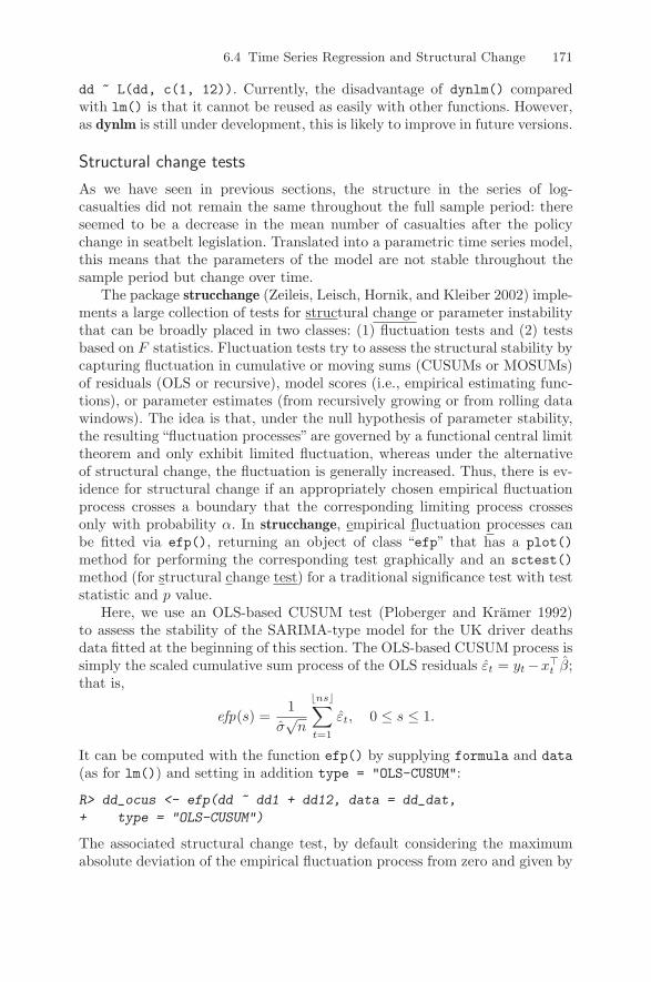
6.4 Time Series Regression and Structural Change 171

dd ~ L(dd, c(1, 12)). Currently, the disadvantage of dynlm() comparedwith lm() is that it cannot be reused as easily with other functions. However,as dynlm is still under development, this is likely to improve in future versions.

Structural change tests

As we have seen in previous sections, the structure in the series of log-casualties did not remain the same throughout the full sample period: thereseemed to be a decrease in the mean number of casualties after the policychange in seatbelt legislation. Translated into a parametric time series model,this means that the parameters of the model are not stable throughout thesample period but change over time.

The package strucchange (Zeileis, Leisch, Hornik, and Kleiber 2002) imple-ments a large collection of tests for structural change or parameter instabilitythat can be broadly placed in two classes: (1) fluctuation tests and (2) testsbased on F statistics. Fluctuation tests try to assess the structural stability bycapturing fluctuation in cumulative or moving sums (CUSUMs or MOSUMs)of residuals (OLS or recursive), model scores (i.e., empirical estimating func-tions), or parameter estimates (from recursively growing or from rolling datawindows). The idea is that, under the null hypothesis of parameter stability,the resulting “fluctuation processes” are governed by a functional central limittheorem and only exhibit limited fluctuation, whereas under the alternativeof structural change, the fluctuation is generally increased. Thus, there is ev-idence for structural change if an appropriately chosen empirical fluctuationprocess crosses a boundary that the corresponding limiting process crossesonly with probability α. In strucchange, empirical fluctuation processes canbe fitted via efp(), returning an object of class “efp” that has a plot()method for performing the corresponding test graphically and an sctest()method (for structural change test) for a traditional significance test with teststatistic and p value.

Here, we use an OLS-based CUSUM test (Ploberger and Kramer 1992)to assess the stability of the SARIMA-type model for the UK driver deathsdata fitted at the beginning of this section. The OLS-based CUSUM process issimply the scaled cumulative sum process of the OLS residuals εt = yt−x>t β;that is,

efp(s) =1

σ√

n

bnsc∑t=1

εt, 0 ≤ s ≤ 1.

It can be computed with the function efp() by supplying formula and data(as for lm()) and setting in addition type = "OLS-CUSUM":

R> dd_ocus <- efp(dd ~ dd1 + dd12, data = dd_dat,

+ type = "OLS-CUSUM")

The associated structural change test, by default considering the maximumabsolute deviation of the empirical fluctuation process from zero and given by

172 6 Time Series

R> sctest(dd_ocus)

OLS-based CUSUM test

data: dd_ocusS0 = 1.4866, p-value = 0.02407

is significant at the default 5% level, signaling that the model parameters arenot stable throughout the entire sample period. The plot in the left panel ofFigure 6.10 results from

R> plot(dd_ocus)

and yields some further insights. In addition to the excessive fluctuation (con-veyed by the boundary crossing), it can be seen from the peak in the processthat an abrupt change seems to have taken place in about 1973(10), match-ing the timing of the first oil crisis. A smaller second peak in the process,associated with the change of seatbelt legislation in 1983(1), is also visible.

Tests based on F statistics, the second class of tests in strucchange, aredesigned to have good power for single-shift alternatives (of unknown tim-ing). The basic idea is to compute an F statistic (or Chow statistic) for eachconceivable breakpoint in a certain interval and reject the null hypothesis ofstructural stability if any of these statistics (or some other functional suchas the mean) exceeds a certain critical value (Andrews 1993; Andrews andPloberger 1994). Processes of F statistics can be fitted with Fstats(), em-ploying an interface similar to efp(). The resulting “Fstats” objects canagain be assessed by the corresponding sctest() method or graphically bythe plot() method. The code chunk

R> dd_fs <- Fstats(dd ~ dd1 + dd12, data = dd_dat, from = 0.1)

R> plot(dd_fs)

R> sctest(dd_fs)

supF test

data: dd_fssup.F = 19.3331, p-value = 0.006721

uses the supF test of Andrews (1993) for the SARIMA-type model with atrimming of 10%; i.e., an F statistic is computed for each potential break-point between 1971(6) and 1983(6), omitting the leading and trailing 10% ofobservations. The resulting process of F statistics is shown in the right panelof Figure 6.10, revealing two clear peaks in 1973(10) and 1983(1). Both theboundary crossing and the tiny p value show that there is significant departurefrom the null hypothesis of structural stability. The two peaks in the F pro-cess also demonstrate that although designed for single-shift alternatives, thesupF test has power against multiple-shift alternatives. In this case, it bringsout the two breaks even more clearly than the OLS-based CUSUM test.

6.4 Time Series Regression and Structural Change 173

Fig. 6.10. OLS-based CUSUM process (left) and process of F statistics (right) forthe UK driver deaths model.

Many further tests for structural change are available in strucchange. Aunified and more flexible approach is implemented in gefp() (Zeileis 2005,2006a). In practice, this multitude of tests is often a curse rather than ablessing. Unfortunately, no test is superior to any other test for all conceivablepatterns of structural change. Hence, the choice of a suitable test can befacilitated if there is some prior knowledge about which types of changes arelikely to occur and which parameters are affected by it (see Zeileis 2005, forsome discussion of this).

To further illustrate the wide variety of structural change tests, we considera second example. Lutkepohl, Terasvirta, and Wolters (1999) establish anerror correction model (ECM) for German M1 money demand, reanalyzed byZeileis, Leisch, Kleiber, and Hornik (2005) in a structural change setting. Thedata frame GermanM1 contains data from 1961(1) to 1995(4) on per capitaM1, price index, per capita GNP (all in logs) and an interest rate. It can beloaded along with the model used by Lutkepohl et al. (1999) via

R> data("GermanM1")

R> LTW <- dm ~ dy2 + dR + dR1 + dp + m1 + y1 + R1 + season

involving the differenced and lagged series as well as a factor season thatcodes the quarter of the year. To test whether a stable model can be fitted forthis ECM, particularly in view of the German monetary unification on 1990-06-01, a recursive estimates (RE) test (the “fluctuation test” of Ploberger,Kramer, and Kontrus 1989), is employed using

R> m1_re <- efp(LTW, data = GermanM1, type = "RE")

R> plot(m1_re)

OLS−based CUSUM test

Time

Em

piric

al fl

uctu

atio

n pr

oces

s

1970 1975 1980 1985

−1.

00.

01.

0supF test

Time

F s

tatis

tics

1972 1976 1980

05

1015

20

174 6 Time Series

Fig. 6.11. Recursive estimates fluctuation process for German M1 model.

The boundary crossing of the RE process shown in Figure 6.11 signals againthat there is a deviation from structural stability (at the default 5% level), andthe clear peak conveys that this is due to an abrupt change in 1990, matchingthe timing of the German monetary unification.

Dating structural changes

Given that there is evidence for structural change in a certain model, a naturalstrategy is to find a model that incorporates the changes. When the changesare abrupt, this amounts to segmenting the original data and fitting the modelon each subset. In the framework of the linear regression model, the setup is

yt = x>t β(j) + εt, t = nj−1 + 1, . . . , nj , j = 1, . . . ,m + 1, (6.4)

where j = 1, . . . ,m is the segment index and β(j) is the segment-specific setof regression coefficients. The indices n1, . . . , nm denote the set of unknownbreakpoints, and by convention n0 = 0 and nm+1 = n.

Estimating the breakpoints is also called dating structural changes. Forthe two models considered above, visual inspection already provides informa-tion on the locations of the breakpoints. However, a more formal procedurefor determining the number and location of breakpoints is desirable. Bai andPerron (1998, 2003) established a general methodology for estimating break-points and their associated confidence intervals in OLS regression, and their

RE test (recursive estimates test)

Time

Em

piric

al fl

uctu

atio

n pr

oces

s

1965 1970 1975 1980 1985 1990 1995

0.0

0.5

1.0

1.5

2.0

6.4 Time Series Regression and Structural Change 175

method is implemented in the function breakpoints() by Zeileis, Kleiber,Kramer, and Hornik (2003). The dating procedure of Bai and Perron (2003)employs a dynamic programming algorithm based on the Bellman principlefor finding those m breakpoints that minimize the residual sum of squares(RSS) of a model with m + 1 segments, given some minimal segment size ofh ·n observations. Here, h is a bandwidth parameter to be chosen by the user.Similar to the choice of trimming for the F statistics-based tests, the minimalproportion of observations in each segment is typically chosen to be 10% or15%. Given h and m, the breakpoints minimizing the RSS can be determined;however, typically the number of breakpoints m is not known in advance. Onepossibility is to compute the optimal breakpoints for m = 0, 1, . . . breaks andchoose the model that minimizes some information criterion such as the BIC.This model selection strategy is also directly available within breakpoints().

Returning to the UKDriverDeaths series, we estimate the breakpoints fora SARIMA-type model with a minimal segment size of 10% using

R> dd_bp <- breakpoints(dd ~ dd1 + dd12, data = dd_dat, h = 0.1)

The RSS and BIC as displayed by plot(dd_bp) are shown in the left panelof Figure 6.12. Although the RSS drops clearly up to m = 3 breaks, the BICis minimal for m = 0 breaks. This is not very satisfactory, as the structuralchange tests clearly showed that the model parameters are not stable. As theBIC was found to be somewhat unreliable for autoregressive models by Baiand Perron (2003), we rely on the interpretation from the visualization of thestructural change tests and use the model with m = 2 breaks. Its coefficientscan be extracted via

R> coef(dd_bp, breaks = 2)

(Intercept) dd1 dd121970(1) - 1973(10) 1.45776 0.117323 0.6944801973(11) - 1983(1) 1.53421 0.218214 0.5723301983(2) - 1984(12) 1.68690 0.548609 0.214166

reflecting that particularly the period after the change in seatbelt legislationin 1983(1) is different from the observations before. The other breakpointis in 1973(10), again matching the timing of the oil crisis and confirmingthe interpretation from the structural change tests. The observed and fittedseries, along with confidence intervals for the breakpoints, are shown in theright panel of Figure 6.12 as generated by

R> plot(dd)

R> lines(fitted(dd_bp, breaks = 2), col = 4)

R> lines(confint(dd_bp, breaks = 2))

Readers are asked to estimate breakpoints for the GermanM1 example in anexercise.

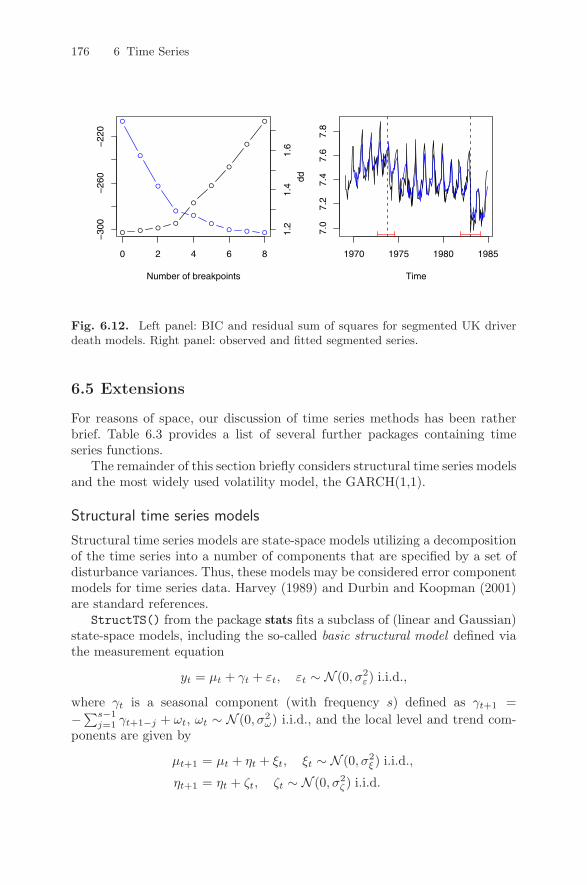
176 6 Time Series

Fig. 6.12. Left panel: BIC and residual sum of squares for segmented UK driverdeath models. Right panel: observed and fitted segmented series.

6.5 Extensions

For reasons of space, our discussion of time series methods has been ratherbrief. Table 6.3 provides a list of several further packages containing timeseries functions.

The remainder of this section briefly considers structural time series modelsand the most widely used volatility model, the GARCH(1,1).

Structural time series models

Structural time series models are state-space models utilizing a decompositionof the time series into a number of components that are specified by a set ofdisturbance variances. Thus, these models may be considered error componentmodels for time series data. Harvey (1989) and Durbin and Koopman (2001)are standard references.

StructTS() from the package stats fits a subclass of (linear and Gaussian)state-space models, including the so-called basic structural model defined viathe measurement equation

yt = µt + γt + εt, εt ∼ N (0, σ2ε) i.i.d.,

where γt is a seasonal component (with frequency s) defined as γt+1 =−

∑s−1j=1 γt+1−j + ωt, ωt ∼ N (0, σ2

ω) i.i.d., and the local level and trend com-ponents are given by

µt+1 = µt + ηt + ξt, ξt ∼ N (0, σ2ξ ) i.i.d.,

ηt+1 = ηt + ζt, ζt ∼ N (0, σ2ζ ) i.i.d.

0 2 4 6 8

−30

0−

260

−22

0

Number of breakpoints

1.

21.

41.

6Time

dd

1970 1975 1980 1985

7.0

7.2

7.4

7.6

7.8

6.5 Extensions 177

Table 6.3. Further packages for time series analysis.

Package Description

dse Multivariate time series modeling with state-space andvector ARMA (VARMA) models (Gilbert 2007).

FinTS R companion to Tsay (2005) with data sets, functions,and script files to work some of the examples (Graves2008).

forecast Univariate time series forecasting, including exponentialsmoothing, state space, and ARIMA models. Part of theforecasting bundle (Hyndman and Khandakar 2008).

fracdiff ML estimation of fractionally integrated ARMA(ARFIMA) models and semiparametric estimation ofthe fractional differencing parameter (Fraley, Leisch, andMaechler 2006).

longmemo Convenience functions for long-memory models; also con-tains several data sets (Beran, Whitcher, and Maechler2007).

mFilter Miscellaneous time series filters, including Baxter-King,Butterworth, and Hodrick-Prescott (Balcilar 2007).

Rmetrics Suite of some 20 packages for financial engineering andcomputational finance (Wuertz 2008), including GARCHmodeling in the package fGarch.

tsDyn Nonlinear time series models: STAR, ESTAR, LSTAR(Di Narzo and Aznarte 2008).

vars (Structural) vector autoregressive (VAR) models (Pfaff2008).

All error terms are assumed to be mutually independent. Special cases are thelocal linear trend model, where γt is absent, and the local linear model, wherein addition σ2

ζ = 0.In total, there are four parameters, σ2

ξ , σ2η, σ2

ω, and σ2ε , some (but not all)

of which may be absent (and often are in practical applications).It should be noted that, for example, the reduced form of the local trend

model is ARIMA(0,2,2), but with restrictions on the parameter set. Propo-nents of structural time series models argue that the implied restrictions oftenare meaningful in practical terms and thus lead to models that are easier tointerpret than results from unrestricted ARIMA fits.

Here, we fit the basic structural model to the UKDriverDeaths data using

R> dd_struct <- StructTS(log(UKDriverDeaths))

178 6 Time Series

Fig. 6.13. The basic structural model for the UK driver deaths.

The resulting components

R> plot(cbind(fitted(dd_struct), residuals(dd_struct)))

are shown in Figure 6.13. This approach also clearly brings out the drop inthe number of accidents in connection with the change in legislation.

More information on structural time series models in R is provided byRipley (2002) and Venables and Ripley (2002).

GARCH models

Many financial time series exhibit volatility clustering. Figure 6.14 provides atypical example, a series of 1974 DEM/GBP exchange rate returns for the

7.1

7.3

7.5

7.7

leve

l

−0.

006

−0.

002

0.00

2

slop

e

−0.

2−

0.1

0.0

0.1

0.2

seas

on

−3

−2

−1

01

23

1970 1975 1980 1985

resi

dual

s

Time

6.5 Extensions 179

Fig. 6.14. DEM/GBP exchange rate returns.

period 1984-01-03 through 1991-12-31, taken from Bollerslev and Ghysels(1996). This data set has recently become a benchmark in the GARCH litera-ture, and it is also used in Greene (2003, Chapter 11). A Ljung-Box test of theMarkPound series suggests that it is white noise (note that this is not withoutproblems since this test assumes i.i.d. data under the null hypothesis), whilea test of the squares is highly significant. Thus, a GARCH model might beappropriate.

The package tseries provides a function garch() for the fitting ofGARCH(p, q) models with Gaussian innovations, defaulting to the popularGARCH(1, 1)

yt = σtνt, νt ∼ N (0, 1) i.i.d.,σ2

t = ω + αy2t−1 + βσ2

t−1, ω > 0, α > 0, β ≥ 0.

For the exchange rate data, we obtain

R> mp <- garch(MarkPound, grad = "numerical", trace = FALSE)

R> summary(mp)

Call:garch(x = MarkPound, grad = "numerical", trace = FALSE)

Model:GARCH(1,1)

Time

Mar

kPou

nd

0 500 1000 1500 2000

−2

−1

01

23

180 6 Time Series

Residuals:Min 1Q Median 3Q Max

-6.79739 -0.53703 -0.00264 0.55233 5.24867

Coefficient(s):Estimate Std. Error t value Pr(>|t|)

a0 0.0109 0.0013 8.38 <2e-16a1 0.1546 0.0139 11.14 <2e-16b1 0.8044 0.0160 50.13 <2e-16

Diagnostic Tests:Jarque Bera Test

data: ResidualsX-squared = 1060.01, df = 2, p-value < 2.2e-16

Box-Ljung test

data: Squared.ResidualsX-squared = 2.4776, df = 1, p-value = 0.1155

which gives ML estimates along with outer-product-of-gradients (OPG) stan-dard errors and also reports diagnostic tests of the residuals for normality (re-jected) and independence (not rejected). Numerical (rather than the defaultanalytical) gradients are employed in the garch() call because the resultingmaximized log-likelihood is slightly larger. For brevity, trace = FALSE sup-presses convergence diagnostics, but we encourage readers to reenable thisoption in applications.

More elaborate tools for volatility modeling are available in the Rmetricscollection of packages (Wuertz 2008). We mention the function garchFit()from the package fGarch, which includes, among other features, a wider se-lection of innovation distributions in GARCH specifications.

6.6 Exercises

1. Decompose the UKNonDurables data. Filter these data using the Holt-Winters technique.

2. Repeat Exercise 1 for the DutchSales data. Compare a decomposition viadecompose() with a decomposition via stl().

3. Using the AirPassengers series,• filter the data using Holt-Winters smoothing,• fit the airline model, and

6.6 Exercises 181

• fit the basic structural model.Compare the results.

4. Reread Nelson and Plosser (1982) and test a selection of the extendedNelson-Plosser data, available as NelPlo in the package tseries, for unitroots. Also fit ARIMA models to these series. (You may need the xregargument to arima() for series that appear to be trend stationary.)

5. Compute and plot the coefficients of the implied MA(∞) representations(i.e., the impulse response functions) for (the stationary part of) the mod-els fitted in the preceding exercise.Hint: Use ARMAtoMA().

6. Stock and Watson (2007) consider an autoregressive distributed lag modelfor the change in the US inflation rate using the USMacroSW data. Specif-ically, the model is

∆inft = β0 +4∑

i=1

βi∆inft−i +4∑

j=1

γjunempt−j + εt.

Plot the sequence of F statistics for a single structural break for thisADL(4, 4) model using Fstats() and test for structural changes with thesupF test.

7. Apply the Bai and Perron (2003) dating algorithm to the German M1data. Do the results correspond to the German monetary reunion?

8. Fit the basic structural model to the UKNonDurables data. Compare thiswith the ARIMA model fitted in Section 6.2.

7

Programming Your Own Analysis

Data analysis, both in academic and in corporate environments, typicallyinvolves, in some form or other, the following three components: (a) usingor writing software that can perform the desired analysis, (b) a sequenceof commands or instructions that apply the software to the data set underinvestigation, and (c) documentation of the commands and their output.

R comes with a rich suite of tools that help implement all these steps whilemaking the analysis reproducible and applicable to new data. So far, we havemostly been concerned with providing short examples of existing functionality.In this chapter, we try to enrich this picture by illustrating how further aspectsof the tasks above can be performed:

(a) In the simplest case, a function that performs exactly the analysis desired isalready available. This is the case for many standard models, as discussedin the preceding chapters. In the worst case, no infrastructure is availableyet, and a new function has to be written from scratch. In most cases,however, something in between is required: a (set of) new function(s) thatreuse(s) existing functionality. This can range from simple convenienceinterfaces to extensions built on top of existing functions. In any case,the resulting software is most easily applicable if the functions reflect theconceptual steps in the analysis.

(b) As R is mostly used via its command-line interface, assembling scripts withR commands is straightforward (and the history() from an R sessionis often a good starting point). To make the results reproducible, it isimportant to keep track of the entire analysis, from data preprocessingover model fitting to evaluation and generation of output and graphics.

(c) For documenting results obtained from an analysis in R, many environ-ments are available, ranging from word processors to markup languagessuch as HTML or LATEX. For all of these it is possible to produce Routput—numerical and/or graphical—and to include this “by hand” in thedocumentation (e.g., by “copy and paste”). However, this can be tediousand, more importantly, make replication or application to a different data

C. Kleiber, A. Zeileis, Applied Econometrics with R,DOI: 10.1007/978-0-387-77318-6 7, © Springer Science+Business Media, LLC 2008

184 7 Programming Your Own Analysis

set much more cumbersome. Therefore, R ships with support for tightlybundling R scripts (as discussed in (b)) and the documentation of theiroutput so that R first runs the analysis and then includes the results in thedocumentation. Base R provides the function Sweave() (in package utils),which by default supports “weaving” of R code with LATEX documentationbut also allows other documentation formats to be plugged in.

In the following, we provide examples for a few typical tasks in econo-metric analysis—simulation of power curves, bootstrapping a regression, andmaximizing a likelihood. In doing so, we go beyond using off-the-shelf softwareand in each case require some of the steps discussed above.

7.1 Simulations

A simulation study is one of the most typical programming tasks when eval-uating some algorithm; e.g., a test procedure or an estimator. It usually in-volves (at least) three steps: (1) simulating data from some data-generatingprocess (DGP); (2) evaluating the quantities of interest (e.g., rejection prob-abilities, parameter estimates, model predictions); and (3) iterating the firsttwo steps over a number of different scenarios. Here, we exemplify how toaccomplish such a task in R by comparing the power of two well-known testsfor autocorrelation—the Durbin-Watson and the Breusch-Godfrey test—intwo different specifications of a linear regression. In the following, we first setup three functions that capture the steps above before we actually run thesimulation and summarize the results both numerically and graphically.

Data-generating process

We consider the Durbin-Watson and Breusch-Godfrey tests for two differentlinear regression models: a trend model with regressor xi = i and a modelwith a lagged dependent variable xi = yi−1. Recall that the Durbin-Watsontest is not valid in the presence of lagged dependent variables.

More specifically, the model equations are

trend: yi = β1 + β2 · i + εi,

dynamic: yi = β1 + β2 · yi−1 + εi,

where the regression coefficients are in both cases β = (0.25,−0.75)>, andεi, i = 1, . . . , n, is a stationary AR(1) series, derived from standard normalinnovations and with lag 1 autocorrelation %. All starting values, both for yand ε, are chosen as 0.

We want to analyze the power properties of the two tests (for size α = 0.05)on the two DGPs for autocorrelations % = 0, 0.2, 0.4, 0.6, 0.8, 0.9, 0.95, 0.99 andsample sizes n = 15, 30, 50.

To carry out such a simulation in R, we first define a function dgp() thatimplements the DGP above:

7.1 Simulations 185

R> dgp <- function(nobs = 15, model = c("trend", "dynamic"),

+ corr = 0, coef = c(0.25, -0.75), sd = 1)

+

+ model <- match.arg(model)

+ coef <- rep(coef, length.out = 2)

+

+ err <- as.vector(filter(rnorm(nobs, sd = sd), corr,

+ method = "recursive"))

+ if(model == "trend")

+ x <- 1:nobs

+ y <- coef[1] + coef[2] * x + err

+ else

+ y <- rep(NA, nobs)

+ y[1] <- coef[1] + err[1]

+ for(i in 2:nobs)

+ y[i] <- coef[1] + coef[2] * y[i-1] + err[i]

+ x <- c(0, y[1:(nobs-1)])

+

+ return(data.frame(y = y, x = x))

+

The arguments to dgp() are nobs (corresponding to n with default 15), model(specifying the equation used, by default "trend"), corr (the autocorrelation%, by default 0), coef (corresponding to β), and sd (the standard deviationof the innovation series). The latter two are held constant in the following.After assuring that model and coef are of the form required, dgp() sets upthe regressor and dependent variable and returns both in a “data.frame”comprising the variables y and x.

Evaluation for a single scenario

Based on this implementation of the DGP, we can now easily simulate thepower of both tests for a given combination of parameters. In simpower(), wejust iterate through a for() loop (by default with nrep = 100 iterations) inwhich we simulate a data set, apply both dwtest() (the Durbin-Watson testfrom lmtest) and bgtest() (the Breusch-Godfrey test from lmtest) to it, andstore the associated p values. After completing the for() loop, we return theproportion of significant p values (by default at size = 0.05).

R> simpower <- function(nrep = 100, size = 0.05, ...)

+

+ pval <- matrix(rep(NA, 2 * nrep), ncol = 2)

+ colnames(pval) <- c("dwtest", "bgtest")

+ for(i in 1:nrep)

+ dat <- dgp(...)

+ pval[i,1] <- dwtest(y ~ x, data = dat,

186 7 Programming Your Own Analysis

+ alternative = "two.sided")$p.value

+ pval[i,2] <- bgtest(y ~ x, data = dat)$p.value

+

+ return(colMeans(pval < size))

+

The remaining argument ... is a simple mechanism for passing on furtherarguments to other functions. Here, any argument beyond nrep and sizeis passed to dgp(). For example, we could easily modify the correlation em-ployed via simpower(corr = 0.9), which would then internally call dgp(corr= 0.9), all other defaults remaining unchanged.

Iterated evaluation over all scenarios

Given these two building blocks, the DGP and the power simulator, we cannow set up the main simulation routine in which we compute the power fordifferent combinations of autocorrelation, sample size, and regression model:

R> simulation <- function(corr = c(0, 0.2, 0.4, 0.6, 0.8,

+ 0.9, 0.95, 0.99), nobs = c(15, 30, 50),

+ model = c("trend", "dynamic"), ...)

+

+ prs <- expand.grid(corr = corr, nobs = nobs, model = model)

+ nprs <- nrow(prs)

+

+ pow <- matrix(rep(NA, 2 * nprs), ncol = 2)

+ for(i in 1:nprs) pow[i,] <- simpower(corr = prs[i,1],

+ nobs = prs[i,2], model = as.character(prs[i,3]), ...)

+

+ rval <- rbind(prs, prs)

+ rval$test <- factor(rep(1:2, c(nprs, nprs)),

+ labels = c("dwtest", "bgtest"))

+ rval$power <- c(pow[,1], pow[,2])

+ rval$nobs <- factor(rval$nobs)

+ return(rval)

+

This function simply sets up all parameter combinations in a “data.frame”using expand.grid() and subsequently simulates both power values for eachof the parameter combinations in a for() loop. Finally, the results are slightlyrearranged and returned in a “data.frame”.

Of course, it would have been possible to code all the preceding steps in asingle function; however, such functions tend to be rather monolithic and notvery intelligible. Encapsulating logical steps in computational building blockshelps to make simulation code readable and facilitates reuse outside a largesimulation. This is particularly helpful during the setup phase, where sanitychecking of the building blocks is possible independently.

7.1 Simulations 187

Simulation and summary

Now, all that is required to run the simulation is to set a random seed(so that the simulation results can always be exactly reproduced) and callsimulation():

R> set.seed(123)

R> psim <- simulation()

Using the default settings, this takes less than a minute on a standard PC;however, the precision from only 100 replications is certainly not sufficient forprofessional applications.

To inspect the simulation results, the most standard and simple format istables with numerical output. Using xtabs(), we can turn the “data.frame”into a “table” that classifies the power outcome by the four design variables.For printing the resulting four-way table, we create a “flat” two-way table.This can be achieved using ftable() (for flat table). Placing the values for %in the columns and nesting all other variables in the rows, we obtain

R> tab <- xtabs(power ~ corr + test + model + nobs, data = psim)

R> ftable(tab, row.vars = c("model", "nobs", "test"),

+ col.vars = "corr")

corr 0 0.2 0.4 0.6 0.8 0.9 0.95 0.99model nobs testtrend 15 dwtest 0.05 0.10 0.21 0.36 0.55 0.65 0.66 0.62

bgtest 0.07 0.05 0.05 0.10 0.30 0.40 0.41 0.3130 dwtest 0.09 0.20 0.57 0.80 0.96 1.00 0.96 0.98

bgtest 0.09 0.09 0.37 0.69 0.93 0.99 0.94 0.9350 dwtest 0.03 0.31 0.76 0.99 1.00 1.00 1.00 1.00

bgtest 0.05 0.23 0.63 0.95 1.00 1.00 1.00 1.00dynamic 15 dwtest 0.02 0.01 0.00 0.00 0.01 0.03 0.01 0.00

bgtest 0.07 0.04 0.01 0.09 0.14 0.21 0.17 0.2630 dwtest 0.00 0.01 0.01 0.06 0.00 0.03 0.03 0.19

bgtest 0.05 0.05 0.18 0.39 0.52 0.63 0.64 0.7450 dwtest 0.02 0.02 0.01 0.03 0.03 0.15 0.39 0.56

bgtest 0.05 0.10 0.36 0.72 0.91 0.90 0.93 0.91

By supplying the test as the last row variable, the table is aimed at comparingthe power curves (i.e., the rejection probabilities for increasing %) between thetwo tests under investigation. It can be seen that the Durbin-Watson testperforms somewhat better in the trend model, although the advantage overthe Breusch-Godfrey test diminishes with increasing % and n. As expected, forthe dynamic model, the Durbin-Watson test has almost no power except forvery high correlations whereas the Breusch-Godfrey test performs acceptably.

This difference becomes even more apparent when the comparison is car-ried out graphically. Instead of the standard R graphics, we prefer to useso-called trellis graphics for this task. R provides the package lattice (Sarkar

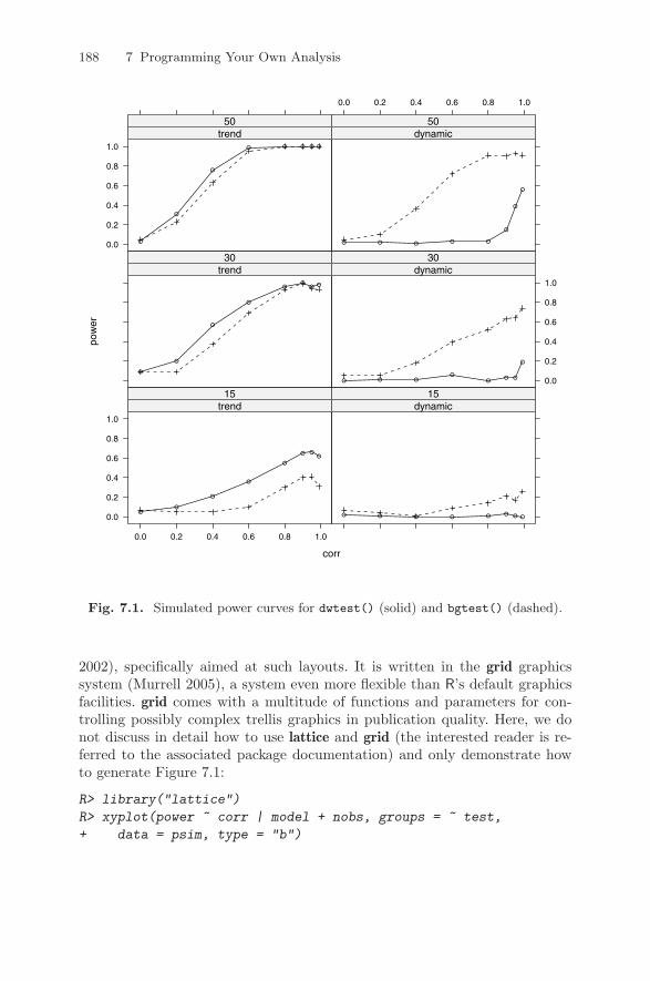
188 7 Programming Your Own Analysis

Fig. 7.1. Simulated power curves for dwtest() (solid) and bgtest() (dashed).

2002), specifically aimed at such layouts. It is written in the grid graphicssystem (Murrell 2005), a system even more flexible than R’s default graphicsfacilities. grid comes with a multitude of functions and parameters for con-trolling possibly complex trellis graphics in publication quality. Here, we donot discuss in detail how to use lattice and grid (the interested reader is re-ferred to the associated package documentation) and only demonstrate howto generate Figure 7.1:

R> library("lattice")

R> xyplot(power ~ corr | model + nobs, groups = ~ test,

+ data = psim, type = "b")

corr

pow

er

0.0

0.2

0.4

0.6

0.8

1.0

0.0 0.2 0.4 0.6 0.8 1.0

trend15

dynamic15

trend30

0.0

0.2

0.4

0.6

0.8

1.0

dynamic30

0.0

0.2

0.4

0.6

0.8

1.0

trend50

0.0 0.2 0.4 0.6 0.8 1.0

dynamic50

7.2 Bootstrapping a Linear Regression 189

Using xyplot(), a trellis scatterplot is generated for power ~ corr condi-tional on the combinations of model and nobs. Within each panel, the obser-vations are grouped by test. All data are taken from the simulation resultspsim, and the plotting type is "b", indicating both (i.e., lines and points). Forfurther control options, see ?xyplot.

In Figure 7.1, rows correspond to varying sample sizes and columns to theunderlying model, and each panel shows the power curves as functions of %for both tests. The interpretation is much easier compared to the numericaltable: power clearly increases with n and %, and autocorrelation is easier todetect in the trend than in the dynamic model. While the Durbin-Watson testperforms slightly better in the trend model for small sample sizes, its powerbreaks down almost completely in the dynamic model.

7.2 Bootstrapping a Linear Regression

Conventional regression output relies on asymptotic approximations to thedistributions of test statistics, which are often not very reliable in small sam-ples or models with substantial nonlinearities. A possible remedy is to employbootstrap methodology.

In R, a basic recommended package is boot (Canty and Ripley 2008), whichprovides functions and data sets from Davison and Hinkley (1997). Specifi-cally, the function boot() implements the classical nonparametric bootstrap(sampling with replacement), among other resampling techniques.

Since there is no such thing as “the” bootstrap, the first question is to de-termine a resampling strategy appropriate for the problem at hand. In econo-metrics and the social sciences, experimental data are rare, and hence it isappropriate to consider regressors as well as responses as random variables.This suggests employing the pairs bootstrap (i.e., to resample observations),a method that should give reliable standard errors even in the presence of(conditional) heteroskedasticity.

As an illustration, we revisit an example from Chapter 3, the Journalsdata taken from Stock and Watson (2007). The goal is to compute bootstrapstandard errors and confidence intervals by case-based resampling. For easeof reference, we reproduce the basic regression

R> data("Journals")

R> journals <- Journals[, c("subs", "price")]

R> journals$citeprice <- Journals$price/Journals$citations

R> jour_lm <- lm(log(subs) ~ log(citeprice), data = journals)

The function boot() takes several arguments, of which data, statistic, andR are required. Here, data is simply the data set and R signifies the numberof bootstrap replicates. The second argument, statistic, is a function thatreturns the statistic to be bootstrapped, where the function itself must take

190 7 Programming Your Own Analysis

the data set and an index vector providing the indices of the observationsincluded in the current bootstrap sample.

This is best understood by considering an example. In our case, the re-quired statistic is given by the convenience function

R> refit <- function(data, i)

+ coef(lm(log(subs) ~ log(citeprice), data = data[i,]))

Now we are ready to call boot():

R> library("boot")

R> set.seed(123)

R> jour_boot <- boot(journals, refit, R = 999)

This yields

R> jour_boot

ORDINARY NONPARAMETRIC BOOTSTRAP

Call:boot(data = journals, statistic = refit, R = 999)

Bootstrap Statistics :original bias std. error

t1* 4.7662 -0.0010560 0.05545t2* -0.5331 -0.0001606 0.03304

A comparison with the standard regression output

R> coeftest(jour_lm)

t test of coefficients:

Estimate Std. Error t value Pr(>|t|)(Intercept) 4.7662 0.0559 85.2 <2e-16log(citeprice) -0.5331 0.0356 -15.0 <2e-16

reveals only minor differences, suggesting that the conventional version is fairlyreliable in this application.

We can also compare bootstrap and conventional confidence intervals. Asthe bootstrap standard errors were quite similar to the conventional ones,confidence intervals will be expected to be quite similar as well in this exam-ple. To save space, we confine ourselves to those of the slope coefficient. Thebootstrap provides the interval

R> boot.ci(jour_boot, index = 2, type = "basic")

7.3 Maximizing a Likelihood 191

BOOTSTRAP CONFIDENCE INTERVAL CALCULATIONSBased on 999 bootstrap replicates

CALL :boot.ci(boot.out = jour_boot, type = "basic", index = 2)

Intervals :Level Basic95% (-0.5952, -0.4665 )Calculations and Intervals on Original Scale

while its classical counterpart is

R> confint(jour_lm, parm = 2)

2.5 % 97.5 %log(citeprice) -0.6033 -0.4628

This underlines that both approaches yield essentially identical results here.Note that boot.ci() provides several further methods for computing boot-strap intervals.

The bootstrap is particularly helpful in situations going beyond least-squares regression; thus readers are asked to explore bootstrap standard errorsin connection with robust regression techniques in an exercise.

Finally, it should be noted that boot contains many further functions forresampling, among them tsboot() for block resampling from time series (forblocks of both fixed and random lengths). Similar functionality is providedby the function tsbootstrap() in the package tseries. In addition, a ratherdifferent approach, the maximum entropy bootstrap (Vinod 2006), is availablein the package meboot.

7.3 Maximizing a Likelihood

Transformations of dependent variables are a popular means to improve theperformance of models and are also helpful in the interpretation of results.Zellner and Revankar (1969), in a search for a generalized production functionthat allows returns to scale to vary with the level of output, introduced (amongmore general specifications) the generalized Cobb-Douglas form

YieθYi = eβ1Kβ2

i Lβ3i ,

where Y is output, K is capital, and L is labor. From a statistical point ofview, this can be seen as a transformation applied to the dependent variableencompassing the level (for θ = 0, which in this application yields the clas-sical Cobb-Douglas function). Introducing a multiplicative error leads to thelogarithmic form

192 7 Programming Your Own Analysis

log Yi + θYi = β1 + β2 log Ki + β3 log Li + εi. (7.1)

However, this model is nonlinear in the parameters, and only for known θcan it be estimated by OLS. Following Zellner and Ryu (1998) and Greene(2003, Chapter 17), using the Equipment data on transportation equipmentmanufacturing, we attempt to simultaneously estimate the regression coeffi-cients and the transformation parameter using maximum likelihood assumingεi ∼ N (0, σ2) i.i.d.

The likelihood of the model is

L =n∏

i=1

φ(εi/σ) · 1 + θYi

Yi

,

where εi = log Yi + θYi − β1 − β2 log Ki − β3 log Li and φ(·) is the probabilitydensity function of the standard normal distribution. Note that ∂εi/∂Yi =(1 + θYi)/Yi.

This gives the log-likelihood

` =n∑

i=1

log(1 + θYi)− log Yi −n∑

i=1

log φ(εi/σ).

The task is to write a function maximizing this log-likelihood with respectto the parameter vector (β1, β2, β3, θ, σ

2). This decomposes naturally into thefollowing three steps: (1) code the objective function, (2) obtain starting valuesfor an iterative optimization, and (3) optimize the objective function using thestarting values.

Step 1: We begin by coding the log-likelihood. However, since the functionoptim() used below by default performs minimization, we have to slightlymodify the natural approach in that we need to minimize the negative of thelog-likelihood.

R> data("Equipment", package = "AER")

R> nlogL <- function(par)

+ beta <- par[1:3]

+ theta <- par[4]

+ sigma2 <- par[5]

+

+ Y <- with(Equipment, valueadded/firms)

+ K <- with(Equipment, capital/firms)

+ L <- with(Equipment, labor/firms)

+

+ rhs <- beta[1] + beta[2] * log(K) + beta[3] * log(L)

+ lhs <- log(Y) + theta * Y

+

+ rval <- sum(log(1 + theta * Y) - log(Y) +

+ dnorm(lhs, mean = rhs, sd = sqrt(sigma2), log = TRUE))

7.3 Maximizing a Likelihood 193

+ return(-rval)

+

The function nlogL() is a function of a vector parameter par comprising fiveelements; for convenience, these are labeled as in Equation (7.1). Variables aretransformed as needed, after which both sides of Equation (7.1) are set up.These ingredients are then used in the objective function rval, the negative ofwhich is finally returned. Note that R comes with functions for the logarithmsof the standard distributions, including the normal density dnorm(..., log= TRUE).

Step 2: optim() proceeds iteratively, and thus (good) starting values areneeded. These can be obtained from fitting the classical Cobb-Douglas formby OLS:

R> fm0 <- lm(log(valueadded/firms) ~ log(capital/firms) +

+ log(labor/firms), data = Equipment)

The resulting vector of coefficients, coef(fm0), is now amended by 0, ourstarting value for θ, and the mean of the squared residuals from the Cobb-Douglas fit, the starting value for the disturbance variance:

R> par0 <- as.vector(c(coef(fm0), 0, mean(residuals(fm0)^2)))

Step 3: We are now ready to search for the optimum. The new vector par0containing all the starting values is used in the call to optim():

R> opt <- optim(par0, nlogL, hessian = TRUE)

By default, optim() uses the Nelder-Mead method, but there are furtheralgorithms available. We set hessian = TRUE in order to obtain standarderrors. Parameter estimates, standard errors, and the value of the objectivefunction at the estimates can now be extracted via

R> opt$par

[1] 2.91469 0.34998 1.09232 0.10666 0.04275

R> sqrt(diag(solve(opt$hessian)))[1:4]

[1] 0.36055 0.09671 0.14079 0.05850

R> -opt$value

[1] -8.939

In spite of the small sample, these results suggest that θ is greater than 0.We add that for practical purposes the solution above needs to be verified;

specifically, several sets of starting values must be examined in order to confirmthat the algorithm did not terminate in a local optimum. McCullough (2004)offers further advice on nonlinear estimation.

Note also that the function presented above is specialized to the dataset under investigation. If a reusable function is needed, a proper function

194 7 Programming Your Own Analysis

GCobbDouglas(formula, data, ...) should be coded and preferably madeavailable in a package (R Development Core Team 2008g), typically the bestmeans of sharing collections of functions.

7.4 Reproducible Econometrics Using Sweave()

As noted above, reproducibility of analyses is crucial, both in academic andcorporate environments (Leisch and Rossini 2003). See McCullough and Vinod(2003), Zeileis and Kleiber (2005), and Koenker and Zeileis (2007) for threerecent examples of partially successful replications in an academic setting. Sev-eral features make R an ideal environment for reproducible research. Firstly, Ris mostly platform independent and runs on Windows, the Mac family of op-erating systems, and various flavors of Unix. Secondly, its open-source naturenot only makes the (binary) system available to everyone but also enables in-spection of the full underlying source code if necessary. Moreover, R supportsliterate programming: Sweave() (Leisch 2002, 2003a) allows for mixing R andLATEX code, making the code and documentation a tightly coupled bundle.

In fact, this book has been entirely written using Sweave() functionality.For compiling a new version of the book, first the whole source code is ex-ecuted, its output (text and graphics) is “weaved” with the LATEX text, andthen pdfLATEX is run to produce the final book in PDF (portable documentformat). Therefore, it is assured that the input and output displayed are al-ways in sync with the versions of the data, code, packages, and R itself. Thewhole process is platform independent—incidentally, the authors simultane-ously used Microsoft Windows, Mac OS X, and Debian GNU/Linux duringthe course of writing this book.

In the following, we illustrate a fairly simple example for mixing R codeand LATEX documentation. We start out from the file Sweave-journals.Rnwdisplayed in Table 7.1.1 It mainly looks like a LATEX file, but it contains R codechunks beginning with <<...>>= and ending in @. This file can be processedby R upon calling

R> Sweave("Sweave-journals.Rnw")

which replaces the original R code by valid LATEX code and weaves it intothe file Sweave-journals.tex shown in Table 7.2. In place of the R chunks,this contains verbatim LATEX chunks with the input and output of the Rcommands and/or an \includegraphics statement for the inclusion offigures generated along the way. The additional environments, such as Sinput,Soutput, and Schunk, are defined in the style file Sweave.sty, a file that ispart of the local R installation. It is included automatically with a system-dependent path. The file Sweave-journals.tex can then be processed asusual by LATEX, producing the final document as shown in Table 7.3.1 The suffix .Rnw is conventionally used to abbreviate “R noweb”. Noweb is a simple

literate-programming tool whose syntax is reused in Sweave().

7.4 Reproducible Econometrics Using Sweave() 195

Table 7.1. A simple Sweave file: Sweave-journals.Rnw.

\documentclass[a4paper]article

\begindocument

We fit a linear regression for the economic journals demand model.

<<>>=

data("Journals", package = "AER")

journals_lm <- lm(log(subs) ~ log(price/citations), data = Journals)

journals_lm

@

A scatter plot with the fitted regression line is shown below.

\begincenter

<<fig=TRUE, echo=FALSE>>=

plot(log(subs) ~ log(price/citations), data = Journals)

abline(journals_lm)

@

\endcenter

\enddocument

In addition to “weaving”, there is a second basic operation for literate-programming documents, called “tangling”, which here amounts to extractingthe included R code. Invoking Stangle() via

R> Stangle("Sweave-journals.Rnw")

produces a file Sweave-journals.R that simply contains the R code from thetwo R chunks.

The basic weaving procedure illustrated above can be refined in manyways. In the starting lines of an R chunk <<...>>=, control options can be in-serted (together with an optional name for the chunk). Above, we already useecho=FALSE (which suppresses the display of the code input) and fig=TRUE(which signals that figures should be produced). By default, both EPS (en-capsulated PostScript) and PDF files are generated so that the associatedLATEX sources can be compiled either with plain LATEX (for DVI documents)or pdfLATEX (for PDF documents). Similarly, many other options can be set,such as height/width for graphics; see ?RweaveLatex for a full list. For run-ning LATEX, the user can, of course, employ any means he or she is accustomedto. However, if desired, running LATEX is also possible from within R by using

196 7 Programming Your Own Analysis

Table 7.2. LATEX file Sweave-journals.tex obtained fromSweave("Sweave-journals.Rnw").

\documentclass[a4paper]article

\usepackage/usr/share/R/share/texmf/Sweave

\begindocument

We fit a linear regression for the economic journals demand model.

\beginSchunk

\beginSinput

R> data("Journals", package = "AER")

R> journals_lm <- lm(log(subs) ~ log(price/citations),

+ data = Journals)

R> journals_lm

\endSinput

\beginSoutput

Call:

lm(formula = log(subs) ~ log(price/citations), data = Journals)

Coefficients:

(Intercept) log(price/citations)

4.766 -0.533

\endSoutput

\endSchunk

A scatter plot with the fitted regression line is shown below.

\begincenter

\includegraphicsSweave-journals-002

\endcenter

\enddocument

the function texi2dvi() from the package tools 2. PDF output can then begenerated by

R> texi2dvi("Sweave-journals.tex", pdf = TRUE)

The source code for the example above is also contained in a so-called vi-gnette (Leisch 2003b) in the folder ~/AER/inst/doc of the AER package. Theassociated PDF document can be viewed by calling2 If texi2dvi() does not work out of the box, it might be necessary to set the"texi2dvi" option, see ?texi2dvi for details.

7.4 Reproducible Econometrics Using Sweave() 197

Table 7.3. Final document created by running LATEX on Sweave-journals.tex.

We fit a linear regression for the economic journals demand model.

R> data("Journals", package = "AER")

R> journals_lm <- lm(log(subs) ~ log(price/citations),

+ data = Journals)

R> journals_lm

Call:

lm(formula = log(subs) ~ log(price/citations), data = Journals)

Coefficients:

(Intercept) log(price/citations)

4.766 -0.533

A scatter plot with the fitted regression line is shown below.

−4 −2 0 2

12

34

56

7

log(price/citations)

log(

subs

)

198 7 Programming Your Own Analysis

R> vignette("Sweave-journals", package = "AER")

This document makes it obvious that it was generated from R because itincludes verbatim R input and output.

For generating reports or papers, one often wants to avoid verbatimsections and use LATEX formulas and equations instead. This is also easilyachieved using Sweave(), while maintaining the dynamic character of thedocument. Two simple ways are to include the output of R expressions di-rectly in the text via \Sexpr or to produce full LATEX code in an R chunk.We use the former for displaying a formula for the journals regression alongwith the estimated coefficients. The LATEX code for this is

\[\log(\textrmsubscriptions) \quad = \quad\Sexprround(coef(journals_lm)[1], digits = 2)\Sexprif(coef(journals_lm)[2] < 0) "-" else "+"\Sexprabs(round(coef(journals_lm)[2], digits = 2))\cdot \log(\textrmprice per citation)

\]

containing three \Sexpr statements: the first and third simply extract andround the coefficients of the fitted“lm”model, and the second one dynamicallychooses the right sign for the slope. The output in the processed document is

log(subscriptions) = 4.77− 0.53 · log(price per citation)

This is very handy for including small text fragments, typically numbers orshort sequences of text. For producing more complex text structures (e.g.,tables), it is often simpler to use the rich text processing functionality (seeChapter 2 and ?paste) and put together the full LATEX code within R.

Here, we produce the usual table of coefficients for a regression model.The code below sets up a table in LATEX, the core of which is filled by theoutput of an R chunk whose output is treated as LATEX code by setting theoption results=tex. It extracts the coefficients table from the summary() ofthe “lm” object, rounds the numbers and coerces them to characters, prettifiesthe p values, and then pastes everything into a LATEX table. The resultingdocument is shown in Table 7.4.

Table 7.4. Regression summary

Estimate Std. error t statistic p value

(Intercept) 4.766 0.056 85.249 < 0.001log(price/citations) -0.533 0.036 -14.968 < 0.001

7.4 Reproducible Econometrics Using Sweave() 199

\begintable\centering\captionRegression summary\begintabularrrrrr\hline& Estimate & Std.~error & $t$ statistic & $p$ value \\\hline<<echo=FALSE, results=tex>>=x <- summary(journals_lm)$coefficientsx[] <- as.character(round(x, digits = 3))x[,4] <- ifelse(as.numeric(x[,4]) < 0.001, "$<$ 0.001", x[,4])cat(paste(rownames(x), "&",apply(x, 1, paste, collapse = " & "), "\\\\ \n"))

@\hline\endtabular\endtable

The last command in the R chunk is somewhat more complex; hence werecommend that readers simply try to put it together step by step. Notethat the backslash \ has to be escaped because it is the escape character.Therefore, to produce a double backslash \\ in cat(), both backslashes haveto be escaped.

Instead of hand-crafting the LATEX summary, similar code could have beengenerated using the xtable package (Dahl 2007), which can export tables forseveral standard R objects to LATEX or HTML.

Although base R just supports weaving of R code and LATEX documenta-tion, Sweave() is written in such a way that it can be extended to other doc-umentation formats as well. The package R2HTML (Lecoutre 2003) providesthe function RweaveHTML(), which allows mixing R code with HTML documen-tation. Similarly, the package odfWeave (Kuhn 2008) contains infrastructurefor embedding R code and output into word-processor files. Specifically, thefunction RweaveOdf() and its wrapper odfWeave() can weave R and text inopen document format (ODF). This is a word-processor format supported byvarious programs, most notably the OpenOffice.org suite, from which ODFfiles can be exported into many other formats, including Microsoft Word doc-uments and rich text format (RTF). See Koenker and Zeileis (2007) for furtherinformation.

200 7 Programming Your Own Analysis

7.5 Exercises

1. Empirical macroeconomics has seen revived interest in filtering techniques.Write a function implementing the filter known as the Hodrick-Prescottfilter among economists, including an estimate of its smoothing parameter.Schlicht (2005) is a good starting point.

2. Our analysis of the OECDGrowth data in Chapter 4 used highly nonlinearrobust regression techniques; in addition, the data set is rather small.(a) Compute bootstrap standard errors as an alternative to the conven-

tional asymptotic approximations.(b) Compare the results in (a) with the standard errors obtained in Chap-

ter 4.3. Zellner and Ryu (1998) also use the Equipment data while discussing a

wider set of functional forms.(a) (optional) Do not use the AER version of the data set. Instead, down-

load these data from the data archive of the Journal of Applied Econo-metrics, where they are ordered by variable. Use the scan() functionto generate a data.frame.

(b) Estimate some of the generalized functional forms considered by Zell-ner and Ryu (1998) via maximum likelihood following the approachoutlined in Section 7.3.

References

Andrews DWK (1991). “Heteroskedasticity and Autocorrelation ConsistentCovariance Matrix Estimation.” Econometrica, 59, 817–858.

Andrews DWK (1993). “Tests for Parameter Instability and StructuralChange with Unknown Change Point.” Econometrica, 61, 821–856.

Andrews DWK, Monahan JC (1992). “An Improved Heteroskedasticity andAutocorrelation Consistent Covariance Matrix Estimator.” Econometrica,60(4), 953–966.

Andrews DWK, Ploberger W (1994). “Optimal Tests When a NuisanceParameter Is Present Only Under the Alternative.” Econometrica, 62,1383–1414.

Anglin PM, Gencay R (1996). “Semiparametric Estimation of a Hedonic PriceFunction.” Journal of Applied Econometrics, 11, 633–648.

Arellano M, Bond S (1991). “Some Tests of Specification for Panel Data:Monte Carlo Evidence and an Application to Employment Equations.” Re-view of Economic Studies, 58, 277–297.

Bai J, Perron P (1998). “Estimating and Testing Linear Models with MultipleStructural Changes.” Econometrica, 66, 47–78.

Bai J, Perron P (2003). “Computation and Analysis of Multiple StructuralChange Models.” Journal of Applied Econometrics, 18, 1–22.

Balcilar M (2007). mFilter: Miscellaneous Time-Series Filters. R packageversion 0.1-3, URL http://CRAN.R-project.org/package=mFilter.

Baltagi BH (2002). Econometrics. 3rd edition. Springer-Verlag, NewYork. URL http://www.springeronline.com/sgw/cda/frontpage/0,10735,4-165-2-107420-0,00.html.

Baltagi BH (2005). Econometric Analysis of Panel Data. 3rd edition.John Wiley & Sons, Hoboken, NJ. URL http://www.wiley.com/legacy/wileychi/baltagi3e/.

Baltagi BH, Khanti-Akom S (1990). “On Efficient Estimation with Panel Data:An Empirical Comparison of Instrumental Variables Estimators.” Journalof Applied Econometrics, 5, 401–406.

202 References

Bates D (2008). lme4: Linear Mixed-Effects Models Using S4 Classes. R pack-age version 0.99875-9, URL http://CRAN.R-project.org/package=lme4.

Becker RA, Chambers JM (1984). S: An Interactive Environment for DataAnalysis and Graphics. Wadsworth and Brooks/Cole, Monterey, CA.

Becker RA, Chambers JM, Wilks AR (1988). The New S Language. Chapman& Hall, London.

Belsley DA, Kuh E, Welsch RE (1980). Regression Diagnostics: IdentifyingInfluential Data and Sources of Collinearity. John Wiley & Sons, New York.

Beran J, Whitcher B, Maechler M (2007). longmemo: Statistics forLong-Memory Processes. R package version 0.9-5, URL http://CRAN.R-project.org/package=longmemo.

Bergstrom TC (2001). “Free Labor for Costly Journals?” Journal of EconomicPerspectives, 15, 183–198.

Berndt ER (1991). The Practice of Econometrics. Addison-Wesley, Reading,MA.

Bierens H, Ginther DK (2001). “Integrated Conditional Moment Testing ofQuantile Regression Models.” Empirical Economics, 26, 307–324.

Bollerslev T, Ghysels E (1996). “Periodic Autoregressive Conditional Het-eroskedasticity.” Journal of Business & Economic Statistics, 14, 139–151.

Box GEP, Jenkins G (1970). Time Series Analysis: Forecasting and Control.Holden-Day, San Francisco.

Box GEP, Pierce DA (1970). “Distribution of Residual Correlations inAutoregressive-Integrated Moving Average Time Series Models.” Journalof the American Statistical Association, 65, 1509–1526.

Breusch TS (1979). “Testing for Autocorrelation in Dynamic Linear Models.”Australian Economic Papers, 17, 334–355.

Breusch TS, Pagan AR (1979). “A Simple Test for Heteroscedasticity andRandom Coefficient Variation.” Econometrica, 47, 1287–1294.

Brockwell PJ, Davis RA (1991). Time Series: Theory and Methods. 2ndedition. Springer-Verlag, New York.

Brockwell PJ, Davis RA (1996). Introduction to Time Series and Forecasting.Springer-Verlag, New York.

Brown RL, Durbin J, Evans JM (1975). “Techniques for Testing the Constancyof Regression Relationships over Time.” Journal of the Royal StatisticalSociety, Series B, 37, 149–163.

Cameron AC, Trivedi PK (1990). “Regression-Based Tests for Overdispersionin the Poisson Model.” Journal of Econometrics, 46, 347–364.

Cameron AC, Trivedi PK (1998). Regression Analysis of Count Data. Cam-bridge University Press, Cambridge.

Canty A, Ripley BD (2008). boot: Functions and Datasets for Bootstrapping.R package version 1.2-33, URL http://CRAN.R-project.org/package=boot.

Chambers JM (1998). Programming with Data. Springer-Verlag, New York.Chambers JM, Hastie TJ (eds.) (1992). Statistical Models in S. Chapman &

Hall, London.

References 203

Cleveland RB, Cleveland WS, McRae J, Terpenning I (1990). “STL: ASeasonal-Trend Decomposition Procedure Based on Loess.” Journal of Of-ficial Statistics, 6, 3–73.

Cleveland WS (1993). Visualizing Data. Hobart Press, Summit, NJ.Cornwell C, Rupert P (1988). “Efficient Estimation with Panel Data: An

Empirical Comparison of Instrumental Variables Estimators.” Journal ofApplied Econometrics, 3, 149–155.

Cribari-Neto F (2004). “Asymptotic Inference Under Heteroskedasticity ofUnknown Form.” Computational Statistics & Data Analysis, 45, 215–233.

Cribari-Neto F, Zarkos SG (1999). “R: Yet Another Econometric ProgrammingEnvironment.” Journal of Applied Econometrics, 14, 319–329.

Croissant Y (2008). mlogit: Multinomial Logit Models with Choice-SpecificVariables. R package version 0.1-0, URL http://CRAN.R-project.org/package=mlogit.

Croissant Y, Millo G (2008). “plm: Linear Models for Panel Data.” Journalof Statistical Software. Forthcoming.

Dahl DB (2007). xtable: Export Tables to LATEX or HTML. R package ver-sion 1.5-2, URL http://CRAN.R-project.org/package=xtable.

Dalgaard P (2002). Introductory Statistics with R. Springer-Verlag, New York.Davidson R, MacKinnon JG (1981). “Several Tests for Model Specification in

the Presence of Alternative Hypotheses.” Econometrica, 49, 781–793.Davidson R, MacKinnon JG (2004). Econometric Theory and Methods. Ox-

ford University Press, Oxford.Davison AC, Hinkley DV (1997). Bootstrap Methods and Their Applications.

Cambridge University Press, Cambridge.Di Narzo AF, Aznarte JL (2008). tsDyn: Time Series Analysis Based on

Dynamical Systems Theory. R package version 0.6-0, URL http://CRAN.R-project.org/package=tsDyn.

Dickey D, Fuller W (1981). “Likelihood Ratio Tests for Autoregressive TimeSeries with a Unit Root.” Econometrica, 49, 1057–1072.

Durbin J, Koopman SJ (2001). Time Series Analysis by State Space Methods.Oxford University Press, Oxford.

Durbin J, Watson GS (1950). “Testing for Serial Correlation in Least SquaresRegression I.” Biometrika, 37, 409–428.

Eicker F (1963). “Asymptotic Normality and Consistency of the Least SquaresEstimator for Families of Linear Regressions.” Annals of MathematicalStatistics, 34, 447–456.

Elliott G, Rothenberg TJ, Stock JH (1996). “Efficient Tests for an Autore-gressive Unit Root.” Econometrica, 64, 813–836.

Engle RF, Granger CWJ (1987). “Co-integration and Error Correction: Rep-resentation, Estimation, and Testing.” Econometrica, 55, 251–276.

Fair RC (1978). “A Theory of Extramarital Affairs.” Journal of PoliticalEconomy, 86, 45–61.

Faraway JJ (2005). Linear Models with R. Chapman & Hall/CRC, BocaRaton, FL.

204 References

Fox J (2002). An R and S-PLUS Companion to Applied Regression. SagePublications, Thousand Oaks, CA.

Fox J (2003). “Effect Displays in R for Generalised Linear Models.” Journalof Statistical Software, 8(15), 1–18. URL http://www.jstatsoft.org/v8/i15/.

Fraley C, Leisch F, Maechler M (2006). fracdiff: Fractionally DifferencedARIMA Models. R package version 1.3-1, URL http://CRAN.R-project.org/package=fracdiff.

Franses PH (1998). Time Series Models for Business and Economic Forecast-ing. Cambridge University Press, Cambridge. URL http://www.few.eur.nl/few/people/franses/research/book2.htm.

Freedman DA (2006). “On the So-Called ‘Huber Sandwich Estimator’ and‘Robust Standard Errors’.” The American Statistician, 60(4), 299–302.

Friendly M (1994). “Mosaic Displays for Multi-Way Contingency Tables.”Journal of the American Statistical Association, 89, 190–200.

Gerfin M (1996). “Parametric and Semi-Parametric Estimation of the Bi-nary Response Model of Labour Market Participation.” Journal of AppliedEconometrics, 11, 321–339.

Gilbert P (2007). dse: Dynamic Systems Estimation. R bundle with pack-ages dse1 and dse2, version 2007.11-1, URL http://CRAN.R-project.org/package=dse.

Godfrey LG (1978). “Testing Against General Autoregressive and Moving Av-erage Error Models when the Regressors Include Lagged Dependent Vari-ables.” Econometrica, 46, 1293–1302.

Goldberg D (1991). “What Every Computer Scientist Should Know AboutFloating-Point Arithmetic.” ACM Computing Surveys, 23, 5–48.

Goldfeld SM, Quandt RE (1965). “Some Tests for Homoskedasticity.” Journalof the American Statistical Association, 60, 539–547.

Graves S (2008). FinTS: Companion to Tsay’s ‘Analysis of Financial TimeSeries’. R package version 0.3-1, URL http://CRAN.R-project.org/package=FinTS.

Greene WH (1993). Econometric Analysis. 2nd edition. Macmillan PublishingCompany, New York.

Greene WH (2003). Econometric Analysis. 5th edition. Prentice Hall, UpperSaddle River, NJ. URL http://pages.stern.nyu.edu/~wgreene/Text/econometricanalysis.htm.

Grothendieck G (2005). dyn: Time Series Regression. R package version 0.2-6,URL http://CRAN.R-project.org/package=dyn.

Grothendieck G, Petzoldt T (2004). “R Help Desk: Date and Time Classes inR.” R News, 4(1), 29–32. URL http://CRAN.R-project.org/doc/Rnews/.

Grunfeld Y (1958). “The Determinants of Corporate Investment.” Unpub-lished Ph.D. dissertation, Department of Economics, University of Chicago.

Gurmu S, Trivedi PK (1996). “Excess Zeros in Count Models for RecreationalTrips.” Journal of Business & Economic Statistics, 14, 469–477.

References 205

Hamilton JD (1994). Time Series Analysis. Princeton University Press,Princeton, NJ.

Hartigan JA, Kleiner B (1981). “Mosaics for Contingency Tables.” In W Eddy(ed.),“Computer Science and Statistics: Proceedings of the 13th Symposiumon the Interface,” pp. 268–273. Springer-Verlag, New York.

Harvey AC (1989). Forecasting, Structural Time Series Models and theKalman Filter. Cambridge University Press, Cambridge.

Harvey AC, Collier P (1977). “Testing for Functional Misspecification in Re-gression Analysis.” Journal of Econometrics, 6, 103–119.

Harvey AC, Durbin J (1986). “The Effects of Seat Belt Legislation on BritishRoad Casualties: A Case Study in Structural Time Series Modelling.” Jour-nal of the Royal Statistical Society, Series A, 149, 187–227. With discussion.

Hastie T (2006). gam: Generalized Additive Models. R package version 0.98,URL http://CRAN.R-project.org/package=gam.

Hastie T, Tibshirani R, Friedman J (2001). The Elements of Statistical Learn-ing. Springer-Verlag, New York.

Hausman JA, Taylor WE (1981). “Panel Data and Unobservable IndividualEffects.” Econometrica, 49, 1377–1398.

Hayfield T, Racine JS (2008). “Nonparametric Econometrics: The np Pack-age.” Journal of Statistical Software. Forthcoming.

Heij C, de Boer PMC, Franses PH, Kloek T, van Dijk HK (2004). EconometricMethods with Applications in Business and Economics. Oxford UniversityPress, Oxford.

Henningsen A (2008). “Demand Analysis with the Almost Ideal Demand Sys-tem in R: Package micEcon.” Journal of Statistical Software. Forthcoming.

Henningsen A, Hamann JD (2007). “systemfit: A Package for EstimatingSystems of Simultaneous Equations in R.” Journal of Statistical Software,23(4), 1–40. URL http://www.jstatsoft.org/v23/i04/.

Honda Y (1985). “Testing the Error Components Model with Non-normalDisturbances.” Review of Economic Studies, 52, 681–690.

Hyndman RJ, Khandakar Y (2008). “Automatic Time-Series Forecasting: Theforecast Package for R.” Journal of Statistical Software. Forthcoming.

Ihaka R, Gentleman R (1996). “R: A Language for Data Analysis and Graph-ics.” Journal of Computational and Graphical Statistics, 5, 299–314.

Johansen S (1991). “Estimation and Hypothesis Testing of CointegrationVectors in Gaussian Vector Autoregressive Models.” Econometrica, 59,1551–1580.

Klein RW, Spady RH (1993). “An Efficient Semiparametric Estimator forBinary Response Models.” Econometrica, 61, 387–421.

Koenker R (1981). “A Note on Studentizing a Test for Heteroscedasticity.”Journal of Econometrics, 17, 107–112.

Koenker R (2005). Quantile Regression. Cambridge University Press,Cambridge.

Koenker R (2008). quantreg: Quantile Regression. R package version 4.17,URL http://CRAN.R-project.org/package=quantreg.

206 References

Koenker R, Hallock KF (2001). “Quantile Regression.” Journal of EconomicPerspectives, 15(4), 143–156.

Koenker R, Zeileis A (2007). “Reproducible Econometric Research (A CriticalReview of the State of the Art).” Report 60, Department of Statistics andMathematics, Wirtschaftsuniversitat Wien, Research Report Series. URLhttp://epub.wu-wien.ac.at/.

Kramer W, Sonnberger H (1986). The Linear Regression Model Under Test.Physica-Verlag, Heidelberg.

Kuhn M (2008). odfWeave: Sweave Processing of Open Document Format(ODF) Files. R package version 0.7.5, URL http://CRAN.R-project.org/package=odfWeave.

Kwiatkowski D, Phillips PCB, Schmidt P, Shin Y (1992). “Testing the NullHypothesis of Stationarity against the Alternative of a Unit Root.” Journalof Econometrics, 54, 159–178.

Lambert D (1992). “Zero-Inflated Poisson Regression, with an Application toDefects in Manufacturing.” Technometrics, 34, 1–14.

Lecoutre E (2003). “The R2HTML Package.” R News, 3(3), 33–36. URLhttp://CRAN.R-project.org/doc/Rnews/.

Leisch F (2002). “Dynamic Generation of Statistical Reports Using LiterateData Analysis.” In W Hardle, B Ronz (eds.), “COMPSTAT 2002 – Proceed-ings in Computational Statistics,” pp. 575–580. Physica Verlag, Heidelberg.

Leisch F (2003a). “Sweave and Beyond: Computations on Text Docu-ments.” In K Hornik, F Leisch, A Zeileis (eds.), “Proceedings of the3rd International Workshop on Distributed Statistical Computing, Vi-enna, Austria,” ISSN 1609-395X, URL http://www.ci.tuwien.ac.at/Conferences/DSC-2003/Proceedings/.

Leisch F (2003b). “Sweave, Part II: Package Vignettes.” R News, 3(2), 21–24.URL http://CRAN.R-project.org/doc/Rnews/.

Leisch F, Rossini AJ (2003). “Reproducible Statistical Research.” Chance,16(2), 46–50.

Li Q, Racine JS (2007). Nonparametric Econometrics. Theory and Practice.Princeton University Press, Princeton, NJ.

Ligges U (2007). Programmieren in R. 2nd edition. Springer-Verlag, Berlin.Ljung GM, Box GEP (1978). “On a Measure of Lack of Fit in Time Series

Models.” Biometrika, 65, 553–564.Long JS, Ervin LH (2000). “Using Heteroscedasticity Consistent Standard

Errors in the Linear Regression Model.” The American Statistician, 54,217–224.

Lumley T, Heagerty P (1999). “Weighted Empirical Adaptive Variance Es-timators for Correlated Data Regression.” Journal of the Royal StatisticalSociety, Series B, 61, 459–477.

Lutkepohl H, Terasvirta T, Wolters J (1999). “Investigating Stability andLinearity of a German M1 Money Demand Function.” Journal of AppliedEconometrics, 14, 511–525.

References 207

MacKinnon JG, White H (1985). “Some Heteroskedasticity-Consistent Covari-ance Matrix Estimators with Improved Finite Sample Properties.” Journalof Econometrics, 29, 305–325.

Maddala GS (2001). Introduction to Econometrics. 3rd edition. John Wiley& Sons, New York.

Maechler M, Rousseeuw P, Croux C, Todorov V, Ruckstuhl A, Salibian-Barrera M (2007). robustbase: Basic Robust Statistics. R package ver-sion 0.2-8, URL http://CRAN.R-project.org/package=robustbase.

Mankiw NG, Romer D, Weil DN (1992). “A Contribution to the Empirics ofEconomic Growth.” Quarterly Journal of Economics, 107, 407–437.

McCullagh P, Nelder JA (1989). Generalized Linear Models. 2nd edition.Chapman & Hall, London.

McCullough BD (2004). “Some Details of Nonlinear Estimation.” In M Alt-man, J Gill, MP McDonald (eds.), “Numerical Issues in Statistical Com-puting for the Social Scientist,” pp. 199–218. John Wiley & Sons, Hoboken,NJ.

McCullough BD, Vinod HD (2003). “Verifying the Solution from a NonlinearSolver: A Case Study.” American Economic Review, 93, 873–892.

Meyer D (2002). “Naive Time Series Forecasting Methods.” R News, 2(2),7–10. URL http://CRAN.R-project.org/doc/Rnews/.

Mroz TA (1987). “The Sensitivity of an Empirical Model of Married Women’sHours of Work to Economic and Statistical Assumptions.” Econometrica,55, 765–799.

Mullahy J (1986). “Specification and Testing of Some Modified Count DataModels.” Journal of Econometrics, 33, 341–365.

Murrell P (2005). R Graphics. Chapman & Hall/CRC, Boca Raton, FL.Murrell P, Ihaka R (2000). “An Approach to Providing Mathematical Anno-

tation in Plots.” Journal of Computational and Graphical Statistics, 9(3),582–599.

Nelder JA, Wedderburn RWM (1972). “Generalized Linear Models.” Journalof the Royal Statistical Society, Series A, 135, 370–384.

Nelson CR, Plosser CI (1982). “Trends and Random Walks in Economic TimeSeries: Some Evidence and Implications.” Journal of Monetary Economics,10, 139–162.

Newey WK, West KD (1987). “A Simple, Positive-Definite, Heteroskedastic-ity and Autocorrelation Consistent Covariance Matrix.” Econometrica, 55,703–708.

Newey WK, West KD (1994). “Automatic Lag Selection in Covariance MatrixEstimation.” Review of Economic Studies, 61, 631–653.

Nonneman W, Vanhoudt P (1996). “A Further Augmentation of the SolowModel and the Empirics of Economic Growth for OECD Countries.” Quar-terly Journal of Economics, 111, 943–953.

Ozuna T, Gomez I (1995). “Specification and Testing of Count Data Recre-ation Demand Functions.” Empirical Economics, 20, 543–550.

208 References

Pfaff B (2006). Analysis of Integrated and Cointegrated Time Series with R.Springer-Verlag, New York.

Pfaff B (2008). “VAR, SVAR and SVEC Models: Implementation Within RPackage vars.” Journal of Statistical Software. Forthcoming.

Phillips PCB, Ouliaris S (1990). “Asymptotic Properties of Residual BasedTests for Cointegration.” Econometrica, 58, 165–193.

Phillips PCB, Perron P (1988). “Trends and Random Walks in MacroeconomicTime Series.” Biometrika, 75, 335–346.

Ploberger W, Kramer W (1992). “The CUSUM Test with OLS Residuals.”Econometrica, 60(2), 271–285.

Ploberger W, Kramer W, Kontrus K (1989). “A New Test for StructuralStability in the Linear Regression Model.” Journal of Econometrics, 40,307–318.

Racine J, Hyndman RJ (2002). “Using R to Teach Econometrics.” Journal ofApplied Econometrics, 17, 175–189.

Ramsey JB (1969). “Tests for Specification Error in Classical Linear LeastSquares Regression Analysis.” Journal of the Royal Statistical Society, Se-ries B, 31, 350–371.

R Development Core Team (2008a). An Introduction to R. R Foundation forStatistical Computing, Vienna, Austria. ISBN 3-900051-12-7, URL http://www.R-project.org/.

R Development Core Team (2008b). R: A Language and Environment forStatistical Computing. R Foundation for Statistical Computing, Vienna,Austria. ISBN 3-900051-07-0, URL http://www.R-project.org/.

R Development Core Team (2008c). R Data Import/Export. R Foundation forStatistical Computing, Vienna, Austria. ISBN 3-900051-10-0, URL http://www.R-project.org/.

R Development Core Team (2008d). R Installation and Administration. RFoundation for Statistical Computing, Vienna, Austria. ISBN 3-900051-09-7, URL http://www.R-project.org/.

R Development Core Team (2008e). R Internals. R Foundation for Sta-tistical Computing, Vienna, Austria. ISBN 3-900051-14-3, URL http://www.R-project.org/.

R Development Core Team (2008f). R Language Definition. R Foundation forStatistical Computing, Vienna, Austria. ISBN 3-900051-13-5, URL http://www.R-project.org/.

R Development Core Team (2008g). Writing R Extensions. R Foundation forStatistical Computing, Vienna, Austria. ISBN 3-900051-11-9, URL http://www.R-project.org/.

Ripley BD (2002). “Time Series in R 1.5.0.” R News, 2(2), 2–7. URL http://CRAN.R-project.org/doc/Rnews/.

Rousseeuw PJ (1984). “Least Median of Squares Regression.” Journal of theAmerican Statistical Association, 79, 871–880.

Sarkar D (2002). “lattice: An Implementation of Trellis Graphics in R.” RNews, 2(2), 19–23. URL http://CRAN.R-project.org/doc/Rnews/.

References 209

Schlicht E (2005). “Estimating the Smoothing Parameter in the So-CalledHodrick-Prescott Filter.” Journal of the Japan Statistical Society, 35,99–119.

Sing T, Sander O, Beerenwinkel N, Lengauer T (2005). “ROCR: VisualizingClassifier Performance in R.” Bioinformatics, 21(20), 3940–3941.

Steel GL, Sussman GJ (1975). “Scheme: An Interpreter for the ExtendedLambda Calculus.” Memo 349, MIT Artificial Intelligence Laboratory.

Stock JH, Watson MW (2007). Introduction to Econometrics. 2nd edition.Addison-Wesley, Reading, MA.

Stokes H (2004). “On the Advantage of Using Two or More EconometricSoftware Systems to Solve the Same Problem.” Journal of Economic andSocial Measurement, 29, 307–320.

Therneau TM, Grambsch PM (2000). Modeling Survival Data. Springer-Verlag, New York.

Tobin J (1958). “Estimation of Relationships for Limited Dependent Vari-ables.” Econometrica, 26, 24–36.

Toomet O, Henningsen A (2008). “Sample Selection Models in R: PackagesampleSelection.” Journal of Statistical Software. Forthcoming.

Trapletti A (2008). tseries: Time Series Analysis and Computational Fi-nance. R package version 0.10-15, URL http://CRAN.R-project.org/package=tseries.

Tsay RS (2005). Analysis of Financial Time Series. 2nd edition. John Wiley& Sons, Hoboken, NJ.

Utts JM (1982). “The Rainbow Test for Lack of Fit in Regression.” Commu-nications in Statistics – Theory and Methods, 11, 1801–1815.

Venables WN, Ripley BD (2000). S Programming. Springer-Verlag, New York.Venables WN, Ripley BD (2002). Modern Applied Statistics with S. 4th

edition. Springer-Verlag, New York.Verbeek M (2004). A Guide to Modern Econometrics. 2nd edition. John Wiley

& Sons, Hoboken, NJ.Vinod HD (2006). “Maximum Entropy Ensembles for Time Series Inference

in Economics.” Journal of Asian Economics, 17(6), 955–978.White H (1980). “A Heteroskedasticity-Consistent Covariance Matrix Estima-

tor and a Direct Test for Heteroskedasticity.” Econometrica, 48, 817–838.Wilkinson GN, Rogers CE (1973). “Symbolic Description of Factorial Models

for Analysis of Variance.” Applied Statistics, 22, 392–399.Wood SN (2006). Generalized Additive Models: An Introduction with R. Chap-

man & Hall/CRC, Boca Raton, FL.Wooldridge JM (2002). Econometric Analysis of Cross-Section and Panel

Data. MIT Press, Cambridge, MA.Wuertz D (2008). Rmetrics: An Environment and Software Collection for

Teaching Financial Engineering and Computational Finance. R packagesfArma, fAsianOptions, fAssets, fBasics, fCalendar, fCopulae, fEcofin, fEx-oticOptions, fExtremes, fGarch, fImport, fMultivar, fNonlinear, fOptions,

210 References

fPortfolio, fRegression, fSeries, fTrading, fUnitRoots, fUtilities, URL http://CRAN.R-project.org/package=Rmetrics.

Zaman A, Rousseeuw PJ, Orhan M (2001). “Econometric Applications ofHigh-Breakdown Robust Regression Techniques.” Economics Letters, 71,1–8.

Zeileis A (2004). “Econometric Computing with HC and HAC CovarianceMatrix Estimators.” Journal of Statistical Software, 11(10), 1–17. URLhttp://www.jstatsoft.org/v11/i10/.

Zeileis A (2005). “A Unified Approach to Structural Change Tests Based onML Scores, F Statistics, and OLS Residuals.” Econometric Reviews, 24(4),445–466.

Zeileis A (2006a). “Implementing a Class of Structural Change Tests: AnEconometric Computing Approach.”Computational Statistics & Data Anal-ysis, 50, 2987–3008.

Zeileis A (2006b). “Object-oriented Computation of Sandwich Estimators.”Journal of Statistical Software, 16(9), 1–16. URL http://www.jstatsoft.org/v16/i09/.

Zeileis A (2008). dynlm: Dynamic Linear Regression. R package version 0.2-0,URL http://CRAN.R-project.org/package=dynlm.

Zeileis A, Grothendieck G (2005). “zoo: S3 Infrastructure for Regular andIrregular Time Series.” Journal of Statistical Software, 14(6), 1–27. URLhttp://www.jstatsoft.org/v14/i06/.

Zeileis A, Hothorn T (2002). “Diagnostic Checking in Regression Relation-ships.” R News, 2(3), 7–10. URL http://CRAN.R-project.org/doc/Rnews/.

Zeileis A, Kleiber C (2005). “Validating Multiple Structural Change Models– A Case Study.” Journal of Applied Econometrics, 20, 685–690.

Zeileis A, Kleiber C, Jackman S (2008). “Regression Models for Count Datain R.” Journal of Statistical Software. Forthcoming.

Zeileis A, Kleiber C, Kramer W, Hornik K (2003). “Testing and Dating ofStructural Changes in Practice.” Computational Statistics & Data Analysis,44(1–2), 109–123.

Zeileis A, Leisch F, Hornik K, Kleiber C (2002). “strucchange: An R Packagefor Testing for Structural Change in Linear Regression Models.” Journalof Statistical Software, 7(2), 1–38. URL http://www.jstatsoft.org/v07/i02/.

Zeileis A, Leisch F, Kleiber C, Hornik K (2005). “Monitoring StructuralChange in Dynamic Econometric Models.” Journal of Applied Economet-rics, 20, 99–121.

Zellner A (1962). “An Efficient Method of Estimating Seemingly UnrelatedRegressions and Tests for Aggregation Bias.” Journal of the American Sta-tistical Association, 57, 348–368.

Zellner A, Revankar N (1969). “Generalized Production Functions.” Reviewof Economic Studies, 36, 241–250.

References 211

Zellner A, Ryu H (1998). “Alternative Functional Forms for Production, Costand Returns to Scale Functions.” Journal of Applied Econometrics, 13,101–127.

Index

abline(), 2, 57

abs(), 17

accuracy, 128

ACF, see autocorrelation

acf(), 158

acf2AR(), 164

acos(), 17

ADF test, see Dickey-Fuller test,augmented

adf.test(), 165

ADL, see distributed lag

AER, see packages

Affairs, see data sets

AIC, see information criteria

AIC(), 59, 161

airline model, 162

AirPassengers, see data sets

all(), 26

all.equal(), 26

alpha blending, 71

analysis of deviance, 130

analysis of variance, 60, 68

ANOVA, see analysis of variance

anova(), 59, 61, 65, 68, 69, 83, 106, 107,109, 116, 130

any(), 26

apply(), 31, 32

apropos(), 12, 13

ar(), 158–160

AR(1) disturbances, 92

Arellano-Bond estimator, 87

arima(), 159–161, 163, 181

ARIMA model, 157

fitting, 160prediction, 162regression terms, 160seasonal, 160, 161, 169, 171, 175selection, 160simulation, 155

arima.sim(), 155, 164arithmetic, 17

vector arithmetic, 18arma(), 159ARMAacf(), 164ARMAtoMA(), 164, 181as.character(), 27as.data.frame(), 27as.matrix(), 27as.numeric(), 27as.ts(), 153as.vector(), 127as.zoo(), 82, 153asin(), 17atan(), 17attach(), 34auto.arima(), 159, 161autocorrelation, 104, 184

autocorrelation function, 158partial autocorrelation function, 158

BankWages, see data setsbarplot(), 44, 49base, see packagesbasic structural model, see structural

time series modelBernoulli distribution, 123

214 Index

beta(), 18bgtest(), 106, 185, 189BIC, see information criteriabinary response model, 123

semiparametric, 144bkde2D(), 6boot(), 188–190boot, see packagesboot.ci(), 191bootstrap, 188Box-Pierce test, 105Box.test(), 105boxcox(), 91boxplot(), 44, 52bptest(), 102breakpoints(), 174, 175Breusch-Godfrey test, 105, 184Breusch-Pagan test, 101bs(), 70

c(), 18, 22ca.jo(), 168canonical parameter, 122car, see packagescat(), 37, 199cbind(), 22censored dependent variables, 141chol(), 21CigarettesB, see data setsclass(), 11, 38, 39cmeans(), 30, 31Cobb-Douglas function, 191coef(), 59, 61, 163coefficients(), 59coeftest(), 73, 107, 110, 130, 149coercion, 27cointegration, 167colMeans(), 30, 31confidence interval, 61

bootstrap, 189confint(), 59, 61confusion matrix, 128, 146contingency table, 50contour(), 7contrast coding, 67contrasts(), 67, 75cooks.distance(), 99cor(), 51correlation coefficient, 51

Pearson, 51Spearman, 51

cos(), 17count data, 132cov.rob(), 113covariance matrix estimation

Bartlett kernel, 110bootstrap covariance matrix

estimation, 189HAC estimator, 109, 166HC estimator, 107Huber-White estimator, 136Newey-West kernel, 110OPG estimator, 137quadratic spectral kernel, 110robust covariance matrix estimation,

136sandwich estimator, 130, 144

covratio(), 99Cox test, see nonnested modelscoxtest(), 91CPS1985, see data setsCPS1988, see data setsCRAN, 8crossprod(), 21CSS, see least-squares methods,

conditional sum of squarescurve(), 45

d(), 170data(), 36, 46data management, 33

foreign binary formats, 36import and export, 35

data setsAffairs, 141–144, 150AirPassengers, 180BankWages, 147–149CigarettesB, 117CPS1985, 3–7, 46–53CPS1988, 54, 65–75, 115–117, 119DoctorVisits, 150DutchSales, 180EmplUK, 87–89Equipment, 192–194, 200GermanM1, 173–175Grunfeld, 84–87, 89–90, 92HousePrices, 91

Index 215

Journals, 1–3, 36, 41–42, 56–65,101–104, 107–108, 188–191

MarkPound, 179MurderRates, 130–132NelPlo, 181OECDGrowth, 111–114, 118, 199Parade2005, 54PepperPrice, 165PSID1976, 150PSID1982, 91, 92PublicSchools, 94–100, 108–110, 118RecreationDemand, 132–141SwissLabor, 124–130, 144–147, 150UKDriverDeaths, 154–156, 169–175,

177UKNonDurables, 152–163, 180, 181USConsump1993, 92USMacroG, 79–83, 104–106, 110USMacroSW, 181

data-generating process, 184decompose(), 155, 180demo(), 13density(), 48, 54det(), 21dev.copy(), 44dev.off(), 44dev.print(), 44development model, 14deviance(), 59, 125dfbeta(), 99dfbetas(), 99dffit(), 99dffits(), 99DGP, see data-generating processdiag(), 22diagnostic plot, 62, 94diagnostic tests, 101Dickey-Fuller test

augmented, 165diff(), 152dim(), 20dir(), 12, 37dispersion parameter, 122, 125dispersiontest(), 134distributed lag, 79

autoregressive, 79, 83dnorm(), 45DoctorVisits, see data setsdse, see packages

dummy variable, 65, 67dump(), 37Durbin-Watson test, 104, 184DutchSales, see data setsdwtest(), 105, 185, 189dyn, see packagesdynamic programming, 175dynamic regression model, 79, 169dynlm(), 79, 169, 170dynlm, see packages

effects, 125average marginal, 125

effects, see packagesefp(), 171, 172eigen(), 21empirical fluctuation process, see

structural changeemployment equation, 88EmplUK, see data setsencompassing test, see nonnested

modelsencomptest(), 83Engle-Granger two-step method, 167Equipment, see data setserror correction model, 168, 173ets(), 156example(), 12exp(), 17expand.grid(), 161, 186exploratory data analysis, 46exponential family, 122, 135exponential smoothing, 155expression(), 45

factor(), 37, 38, 49, 71false positive rate, 128FAQ, 13fGarch, see packagesFGLS, see least-squares methodsfile(), 37file.copy(), 37file.remove(), 37filter, 154

linear, 154moving average, 154recursive, 154

filter(), 154FinTS, see packages

216 Index

Fisher scoring, 123fitted(), 59fitted.values(), 59five-number summary, 48fivenum(), 48fixed effects, 84fixef(), 85flow control, 28fluctuation test, see structural changefor(), 29, 161, 185, 186forecast, see packagesforecasting, see packagesforeign, see packagesformula, 32, 33fracdiff, see packagesFstats(), 172, 181ftable(), 187function, 9, 11

generic, 11, 38functional form, 103

test for, 103

gam, see packagesgamma(), 18garch(), 179, 180GARCH model, 178garchFit(), 180gefp(), 172generalized linear model, 121, 122, 133geometric distribution, 135GermanM1, see data setsgetwd(), 12GLM, see generalized linear modelglm(), 121, 123, 124, 131, 138glm.nb(), 135GLS, see least-squares methodsgls(), 92Goldfeld-Quandt test, 102gqtest(), 102graphics, 41

colors, 44graphical parameters, 42graphics devices, 44mathematical annotation, 44plotting symbols, 44trellis graphics, 41, 187

gray(), 71grep(), 37grid, see packages

growth regression, 111Grunfeld, see data setsgsub(), 37

HAC estimator, see covariance matrixestimation

Harvey-Collier test, 104harvtest(), 104hat matrix, 97hatvalues(), 97Hausman test, 87Hausman-Taylor model, 87, 92HC estimator, see covariance matrix

estimationhead(), 47heatmap, 6hedonic regression, 91help(), 12, 13help.search(), 12, 13heteroskedasticity, 75, 101hist(), 44histogram, 48history(), 183HoltWinters(), 156HousePrices, see data setshurdle(), 140hurdle model, 139

I(), 66, 68, 91identical(), 26ifelse(), 29image(), 7influence.measures(), 99, 118information criteria

AIC, 149, 160BIC, 162, 175

install.packages(), 9installation, 8instrumental variable, 92interaction, 72, 73is.character(), 27is.na(), 38is.numeric(), 27ivreg(), 92IWLS, see least-squares methods

J test, see nonnested modelsjitter, 71Johansen test, 169

Index 217

Journals, see data setsjtest(), 91

kernel density estimation, 5, 48kernHAC(), 110KernSmooth, see packagesKlein-Spady estimator, 144KPSS test, see stationarity test, KPSSkpss.test(), 167kronecker(), 21

L(), 170labor force participation, 124LAD regression, see quantile regressionlag(), 152, 169, 170lapply(), 32, 70LATEX, 183, 194lattice, see packagesleast absolute deviation regression, see

quantile regressionleast-squares methods

conditional sum of squares, 160feasible generalized least squares

(FGLS), 76generalized least squares (GLS), 76iterated FGLS, 77iterative weighted least squares

(IWLS), 123, 131ordinary least squares (OLS), 2, 4, 11,

55–60, 78–82, 84, 85, 160, 169–171two-stage least squares, 90weighted least squares (WLS), 75–78

legend(), 43length(), 18leverage, 97library(), 8license, 8, 15likelihood, 127, 132, 136, 139–141, 144,

191linear hypothesis, 63linear regression, 2, 3, 55–60, 78–82,

169–171model diagnostics, 94model fitting, 2, 11, 57ordinary least squares (OLS), see

least-squares methodsresiduals, see residuals

linear.hypothesis(), 63–65, 130lines(), 43, 48, 62, 152

link function, 122canonical link function, 122, 133

list(), 24literate programming, 194Ljung-Box test, 105, 162lm(), 2, 4, 6, 33, 55–58, 62, 66, 70, 74,

75, 78, 79, 91, 123, 142, 169–171lme4, see packagesLMS regression, see resistant regressionlmtest, see packagesload(), 12, 36loess smoothing, 155log(), 11, 17, 18log10(), 18log2(), 18logical comparisons, 25logit model, 124, 130logLik(), 59, 127, 163longmemo, see packagesloop, 28, 30lower.tri(), 22lqs(), 112, 113ls(), 10LTS regression, see resistant regression

mahalanobis(), 113main effect, 72MarkPound, see data setsMASS, see packagesmathematical functions, 17matrix operations, 20max(), 17, 48maximum likelihood, 123, 144, 160, 191

nonexistence of estimator, 132MCD, see minimum covariance

determinantmean(), 31meboot, see packagesmerge(), 81, 170methods(), 38, 40mFilter, see packagesmgcv, see packagesmicEcon, see packagesmin(), 17, 48minimum covariance determinant

(MCD) estimator, 113minimum volume ellipsoid (MVE)

estimator, 113missing values, 38

218 Index

ML, see maximum likelihoodmlogit, see packagesmode, 23model comparison, 68money demand, 173mosaic plot, 50multinom(), 148, 149multinomial logit model, 147, 148multinomial response, 147MurderRates, see data setsMVE, see minimum volume ellipsoid

NA, see missing valuesna.omit(), 94ncol(), 20negative binomial distribution, 135negative binomial regression, 134, 135negative.binomial(), 135NelPlo, see data setsnested coding, 72Newey-West estimator, see covariance

matrix estimationNeweyWest(), 110nlme, see packagesnlogL(), 193nnet(), 148nnet, see packagesnonnested models, 82

Cox test, 82encompassing test, 82J test, 82

np, see packagesnpindex(), 146npindexbw(), 145nrow(), 20

object, 9object orientation, 38, 39objects(), 10, 11odfWeave(), 199odfWeave, see packagesOECDGrowth, see data setsOLS, see least-squares methodsoptim(), 192, 193optimization, 191options(), 12ordered probit model, 149ordinal response, 149overdispersion, 133, 135, 136

PACF, see autocorrelationpacf(), 158packages, 8

AER, vi, vii, 1, 4, 9, 36, 38, 41, 64,69, 70, 84, 92, 106, 111, 134, 141,165, 196, 200

base, 10, 12boot, 188, 191car, 63dse, 177dyn, 79dynlm, 79, 169, 171effects, 127fGarch, 177, 180FinTS, 177forecast, 156, 159, 161, 177forecasting, 177foreign, 36fracdiff, 177gam, 145grid, 41, 188KernSmooth, 6lattice, 41, 187, 188lme4, 145lmtest, 69, 83, 91, 101, 105, 107, 185longmemo, 177MASS, 91, 112, 113, 135, 149meboot, 191mFilter, 177mgcv, 145micEcon, 145mlogit, 145, 149nlme, 92nnet, 148np, 71, 144, 147odfWeave, 199plm, 84, 87, 92pscl, 138, 140quantreg, 4, 115–117R2HTML, 199Rmetrics, 177, 180robustbase, 145ROCR, 128sampleSelection, 145sandwich, 94, 106, 110, 136splines, 70stats, 105, 159, 164, 176strucchange, 13, 171, 172survival, 141

Index 219

systemfit, 89, 90tools, 196tsDyn, 177tseries, 159, 164, 166, 167, 179, 181,

191urca, 167, 168utils, 184vars, 177VR, 148xtable, 199zoo, 82, 153

panel data, 84panel regression

dynamic, 87static, 84

par(), 42, 43, 62Parade2005, see data setspartially linear model, 69paste(), 37pdf(), 44, 71PepperPrice, see data setspFtest(), 85pgmm(), 88Phillips-Perron test, 166phtest(), 87pie(), 44, 49pie chart, 44, 49plm(), 84plm, see packagesplm.data(), 84, 89plmtest(), 87plot(), 11, 41–44, 59, 62, 79, 82, 95,

117, 152, 171, 172po.test(), 167points(), 43Poisson distribution, 122, 133, 135Poisson regression, 133polr(), 149power curve, 187, 188PP.test(), 166pp.test(), 166predict(), 4, 56, 59, 61, 127, 139, 163prediction, 61, 127prediction(), 128prediction interval, 61print(), 41, 59, 163probit model, 124, 125, 146production function, 191prop.table(), 49

proportional odds logistic regression,149

pscl, see packagespseudo-R2, 127PSID1976, see data setsPSID1982, see data setsPublicSchools, see data sets

q(), 12QQ plot, 52, 62, 95qqplot(), 44qr(), 21quantile(), 48quantile regression, 4, 115

LAD regression, 115quantreg, see packagesquartz(), 71quasi-Poisson model, 134

R2HTML, see packagesrainbow test, 103raintest(), 103random effects, 85random number generation, 27random seed, 27, 187rbind(), 22read.csv(), 35read.csv2(), 35read.dta(), 36read.table(), 35, 36receiver operating characteristic, 128,

129RecreationDemand, see data setsrecursive estimates test, see structural

changereference category, 67, 75regression diagnostics, 94regression quantiles, see quantile

regressionrelevel(), 75remove(), 10reproducibility, 194reserved words, 32RESET, 103resettest(), 103resid(), 59residuals, 59, 94, 95, 129

deviance, 129Pearson, 129

220 Index

recursive, 104standardized, 97studentized, 99

residuals(), 56, 59, 129resistant regression

LMS regression, 111LTS regression, 111

rgb(), 71RGB color model, 71rm(), 10Rmetrics, see packagesrnorm(), 24, 27, 28, 40robust regression, see resistant

regressionrobustbase, see packagesROC, see receiver operating character-

isticROCR, see packagesrollapply(), 154rq(), 4, 6, 115, 116rstandard(), 97rstudent(), 99rug(), 42RweaveHTML(), 199RweaveOdf(), 199

sample(), 28sampleSelection, see packagessandwich(), 136sandwich, see packagessandwich estimator, see covariance

matrix estimationsapply(), 32SARIMA, see ARIMA, seasonalsave(), 12scale-location plot, 63, 95scan(), 35, 200scatterplot, 41, 51, 94sctest(), 171, 172seemingly unrelated regressions, 89separation, (quasi-)complete, 130–132set.seed(), 27setwd(), 12sign(), 17simulation, 184, 187sin(), 17single-index model, 144sink(), 37skedastic function, 76

Solow model, 111solve(), 21spine plot, 50, 125, 147spinogram, 125spline, 70

B spline, 70cubic spline, 70

splines, see packagessprintf(), 37sqrt(), 17standard errors, see covariance matrix

estimationStangle(), 195stationarity test

KPSS, 167stats, see packagesstl(), 155, 180str(), 41, 46, 47, 152string manipulation, 36strsplit(), 37strucchange, see packagesStructTS(), 158, 159, 176structural change

Chow test, 172CUSUM test, 171, 172dating, 174empirical fluctuation process, 171fluctuation test, 173recursive estimates test, 173supF test, 172tests for structural change, 171

structural time series model, 176basic structural model, 177

structure(), 70subset(), 35subsetting, 19, 24Subversion, 14summary(), 4, 11, 38–41, 47, 56, 58, 59,

63, 73, 74, 85, 90, 106–108, 117,133, 148, 149, 152, 199

summary.default(), 39, 40summary.factor(), 40supF test, see structural changeSUR, see seemingly unrelated regressionsurvival, see packagessurvreg(), 141svd(), 21Sweave(), vi, 184, 194, 198, 199SwissLabor, see data sets

Index 221

system(), 37system.time(), 30systemfit(), 89, 90systemfit, see packages

table(), 50tail(), 47tan(), 17tapply(), 32, 52task view, 9texi2dvi(), 196text(), 43, 45time(), 152time series, 78, 151

classes, 151decompositions, 155diagnostics, 162

tobit(), 141–143tobit model, 141tools, see packagestrue positive rate, 128ts(), 152ts.intersect(), 170ts.union(), 170tsboot(), 191tsbootstrap(), 191tsdiag(), 162tsDyn, see packagestseries, see packagestwo-stage least squares, see least-squares

methods

UKDriverDeaths, see data setsUKNonDurables, see data setsunderdispersion, 134unique(), 113unit root, 165

tests, 165, 166update(), 69, 127upper.tri(), 22ur.ers(), 167urca, see packagesUSConsump1993, see data setsUseMethod(), 39USMacroG, see data setsUSMacroSW, see data setsutils, see packages

VAR, see vector autoregressive modelvariance function

linear, 134NB1, 134NB2, 134quadratic, 134

vars, see packagesvcov(), 59, 107, 137, 163vcovHAC(), 106, 110vcovHC(), 106, 107vector, 23

character, 23logical, 23mode, 23

vector autoregressive model, 168vectorized calculations, 31version control, 14vignette(), 13volatility model, 178VR, see packages

wage equation, 3, 65, 115waldtest(), 69, 83, 107, 109, 110, 130weave(), 110which(), 26which.max(), 26which.min(), 26while(), 29Wilkinson-Rogers notation, 58, 67window(), 152windows(), 71with(), 35WLS, see least-squares methodsword processor, 183write.csv(), 35write.csv2(), 35write.dta(), 36write.table(), 35, 36writeLines(), 37writing functions, 29

xtable, see packagesxtabs(), 50, 187xyplot(), 188

Yule-Walker estimator, 160

zero-inflation model, 137ZINB, 138ZIP, 138

zeroinfl(), 138zoo, see packages

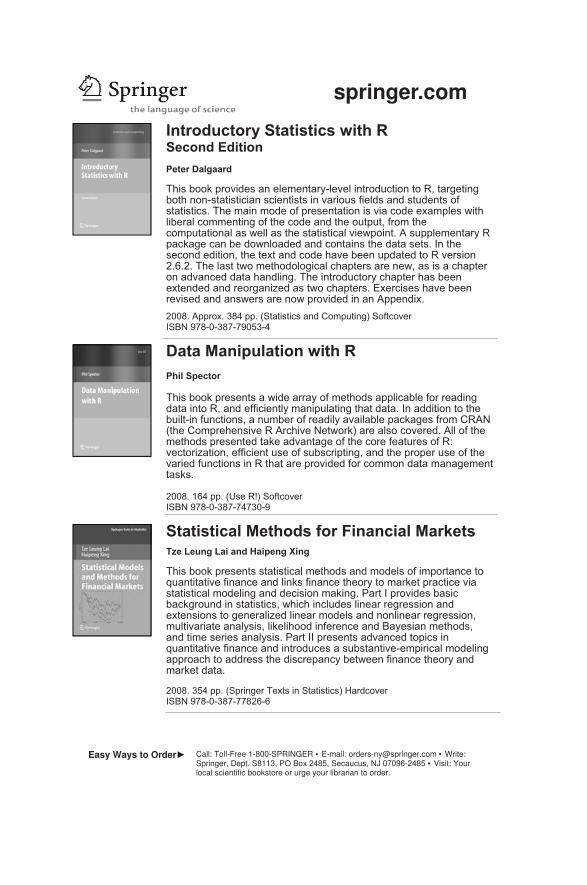
springer.com

Introductory Statistics with R Second Edition Peter Dalgaard This book provides an elementary-level introduction to R, targeting both non-statistician scientists in various fields and students of statistics. The main mode of presentation is via code examples with liberal commenting of the code and the output, from the computational as well as the statistical viewpoint. A supplementary R package can be downloaded and contains the data sets. In the second edition, the text and code have been updated to R version 2.6.2. The last two methodological chapters are new, as is a chapter on advanced data handling. The introductory chapter has been extended and reorganized as two chapters. Exercises have been revised and answers are now provided in an Appendix.

2008. Approx. 384 pp. (Statistics and Computing) Softcover ISBN 978-0-387-79053-4

Data Manipulation with R Phil Spector This book presents a wide array of methods applicable for reading data into R, and efficiently manipulating that data. In addition to the built-in functions, a number of readily available packages from CRAN (the Comprehensive R Archive Network) are also covered. All of the methods presented take advantage of the core features of R: vectorization, efficient use of subscripting, and the proper use of the varied functions in R that are provided for common data management tasks. 2008. 164 pp. (Use R!) Softcover ISBN 978-0-387-74730-9

Statistical Methods for Financial Markets

Tze Leung Lai and Haipeng Xing This book presents statistical methods and models of importance to quantitative finance and links finance theory to market practice via statistical modeling and decision making. Part I provides basic background in statistics, which includes linear regression and extensions to generalized linear models and nonlinear regression, multivariate analysis, likelihood inference and Bayesian methods, and time series analysis. Part II presents advanced topics in quantitative finance and introduces a substantive-empirical modeling approach to address the discrepancy between finance theory and market data. 2008. 354 pp. (Springer Texts in Statistics) Hardcover ISBN 978-0-387-77826-6

Easy Ways to Order Call: Toll-Free 1-800-SPRINGER E-mail: orders-ny@springer.com Write: Springer, Dept. S8113, PO Box 2485, Secaucus, NJ 07096-2485 Visit: Your local scientific bookstore or urge your librarian to order.