user manual m2 mining minima software for host … · user manual m2 mining minima software for...

USER MANUALM2 Mining Minima Software for Host-Guest

BindingVersion 2.A.2 (beta)

Sarvin [email protected]

andMichael K. Gilson

[email protected]

Center for Advanced Research in BiotechnologyUniversity of Maryland Biotechnology Institute

Rockville, MD 20850

c©University of Maryland Biotechnology Institute. August 24, 2009

Contents

Contents i

1 Introduction 1

2 Overview 2

3 Installation 6

3.1 System preparation . . . . . . . . . . . . . . . . . . . . . . . . . . . . 6

3.2 Installation of third party packages . . . . . . . . . . . . . . . . . . . 6

3.3 Installation of M2 codes . . . . . . . . . . . . . . . . . . . . . . . . . 8

4 Tutorial: A Sample M2 Calculation 11

4.1 Procedure . . . . . . . . . . . . . . . . . . . . . . . . . . . . . . . . . 11

5 User Interface Components - M2 Steps 17

5.1 Shared GUI components . . . . . . . . . . . . . . . . . . . . . . . . . 18

5.2 Energy minimization . . . . . . . . . . . . . . . . . . . . . . . . . . . 20

5.3 Tork conformational search . . . . . . . . . . . . . . . . . . . . . . . . 22

5.4 Conformational filtering . . . . . . . . . . . . . . . . . . . . . . . . . 25

5.5 Free energy calculation . . . . . . . . . . . . . . . . . . . . . . . . . . 27

5.6 Free energy correction . . . . . . . . . . . . . . . . . . . . . . . . . . 29

6 User Interface Components - Tools 32

7 M2 Files: Contents and Format 36

i

ii CONTENTS

8 Compilation and Automation 38

9 Tips and Troubleshooting 40

List of Figures

5.1 Main M2 window, with cucurbituril-guest complex. . . . . . . . . . . 17

5.2 Dialog box to load a single molecule or a complex. . . . . . . . . . . . . 18

5.3 Dialog box to set energy minimization parameters. . . . . . . . . . . . . 21

5.4 Dialog box to set Generalized Born parameters. . . . . . . . . . . . . . . 21

5.5 User interface for the Tork conformational search step. . . . . . . . . . . 22

5.6 Dialog box to set Tork conformational search parameters. . . . . . . . . 22

5.7 User interface for conformational filtering. . . . . . . . . . . . . . . . . 25

5.8 User interface for free energy calculation step. . . . . . . . . . . . . . . . 27

5.9 Dialog box to set parameters for free energy calculation step. . . . . . . . 27

5.10 User interface to correct free energies with PB/SA solvation model. . . . . 29

5.11 Dialog box to set parameters for Poisson-Boltzmann solvation calculations. 29

5.12 Dialog box to set parameters for nonpolar solvation component. . . . . . . 30

6.1 User interface for manual docking of guest into host binding site. . . . . . 33

iii

Chapter 1

Introduction

The second-generation version of Mining Minima, M2, provides a systematicmethod for calculating the binding affinities of host-guest systems by computing thestandard chemical potentials of the free host, the free guest, and their complex, andtaking the difference to obtain the standard free energy of binding. M2 relies onthe predominant states approximation (1; 2) to estimate the configuration integralof a molecule or complex as a sum of contributions from its local energy minima;i.e., its low energy conformations. The potential energies of the host and guest areestimated with an empirical force field. In order to reduce the number of degrees offreedom, and hence of local energy minima, the solvation free energy is estimatedwith an implicit solvent model. The free energy of each energy well is estimatedwith the harmonic approximation (HA), adjusted for potential anharmonicities bythe Mode Scanning approach (3).

Chapter 2 of this manual summarizes the theory underlying the method. Chap-ter 3 presents the instructions for installing the components required for running M2.Chapter 4 goes through the steps for computing the binding affinity of a host-guestsystem with sample files provided along with the software. Chapters 5 and 6 providegreater detail regarding the user interface components of the M2 software. Chap-ter 8 provides detailed information about compiling the source code, and Chapter 9provides tips for avoiding pitfalls and getting meaningful results from M2 calcula-tions.

1

Chapter 2

Overview

The M2 method computes the free energy of host-guest binding as

(2.1) ∆G◦ = µocomplex − µo

host − µoguest,

where µocomplex, µo

host, and µoguest are the standard chemical potentials of the com-

plex, host, and guest molecules, respectively. The standard chemical potential of amolecule in solution is approximated as a sum over M local energy minima:

(2.2) µo ≈ −RT ln

(8π2

Co

)−RT ln

M∑i

zi,

where

(2.3) zi =

∫

i

e−E(r)/RT dr,

and R, T , Co, E(r), and zi are, respectively, the gas constant, the absolute tempera-ture, the standard concentration, the energy as a function of the internal coordinatesr, and the configuration integral over internal coordinates in energy well i. (Factorsthat will cancel in the final free energy difference have been omitted.) Local energyminima are identified with the Tork search algorithm (4) (carried out by executableM2 1win.exe or M2 1.exe), and local configuration integrals are computed withthe Harmonic Approximation/Mode Scanning (HA/MS) method (3) (M2 2win.exe

or M2 2.exe). Because the Tork search can arrive at the same conformation morethan once, duplicate conformations are eliminated with a symmetry-aware algorithmto prevent double-counting (5) (chkconf1c-win.exe or chkconf1c-win.exe).

For a molecule or complex with N atoms, the HA/MS method works by di-agonalizing the Cartesian Hessian matrix of the energy at a local energy minimum

2

3

to obtain 3N − 6 Cartesian modes, each comprising an eigenvalue and an eigen-vector. The modes can then be used to approximate the Boltzmann distributionin the energy well as a multidimensional Gaussian with principal axes equal to theeigenvectors and standard deviations along these axes directly related to the corre-sponding eigenvalues. The free energy of the well is then estimated as sum of 3N−6contributions from the respective modes (3). The software starts by projecting theeigenvectors onto Bond-Angle-Torsion coordinates (3). It then estimates the free en-ergy of the well by integrating the Boltzmann distribution along each mode, limitingthe domain of the integral to the lesser of ± 3 standard deviations of the Gaussianalong the mode or that distance which causes any torsion angle to change by morethan 60◦ (6). A number of modes (defined by the user - See Section 5.5) with thelowest force constants are also “scanned” to check and correct for anharmonicity,as follows. For each scanned mode, the scan starts at the local energy minimum,and distorts the molecule along the Bond-Angle-Torsion eigenvector in small stepsuntil the integration limits described above are reached. At each step, the energyand Boltzmann factor are calculated. This scan is done in the positive and negativedirection along the mode. The trapezoid rule is then used to estimate the integralof the Boltzmann factor along the mode, and this scanned integral is compared withthe harmonic one already obtained (above). If the absolute value of the difference isgreater than a cutoff value of 0.5 kcal/mol, then the scanned value is used in place ofthe harmonic value. The free of the energy well j is thus estimated as a sum of con-tributions from each mode, where most modes end up being treated harmonically,while a few that prove to be anharmonic, based on their mode scans, are treatedby the scanning method. Note that this empirical approach does not account forany anharmonicity that may be associated with distortions along combinations ofmodes.

The energy E(r) can be decomposed into the sum of the potential energy,U(r), and the solvation energy, W (r), both functions of the conformation r (7; 8).M2 approximates the potential energy with an empirical force field which, in thepresent implementation, must follow the same widely used functional form found incurrent versions of, for example, CHARMM (9; 10; 11; 12) and AMBER (13; 14).During conformational search and HA/MS calculations, a generalized Born model(15; 16) is used for the solvation energy. Solvation energies are subsequently cor-rected toward the Poisson-Boltzmann/Surface Area model (17; 18), based uponone finite-difference solution of the linearized Poisson-Boltzmann equation and onesurface area calculation for each energy minimum i, as previously described (19)(m2uhbd-win.exe or m2uhbd.exe, obtainable from Prof. James Briggs, U. of Hous-ton).

The M2 calculations also yield an estimate of the change in the Boltzmann-averaged sum of the potential and the solvation energies on binding, ∆〈U + W 〉.

4 CHAPTER 2. OVERVIEW

For this purpose, each energy is considered to be purely harmonic in form, so thatequipartition applies. Thus, if the energy at the base of energy well i is Ui + Wi,then the mean energy in the well is approximated as

(2.4) 〈U + W 〉i = Ui + Wi +3N − 6

2RT

where the third term is the equipartition contribution, Eeq. The mean across all Menergy wells then is

(2.5) 〈U + W 〉 =

∑Mi zi(Ui + Wi)∑M

i zi

+3N − 6

2RT

Applying this expression to the host, the guest, and their complex, yields that

(2.6) ∆〈U + W 〉 = ∆

[∑Mi zi(Ui + Wi)∑M

i zi

]+ 3RT

where ∆ implies the difference between the complex and free species. The 3RTcorrection usually is small in relation to the other quantities and is often neglected.

The estimated change in mean energy provided by Equation 2.6 can be com-bined with the change in binding free energy to yield the change in configurationalentropy (7), which accounts for changes in the mobility of the host and guest onbinding, ∆S◦config:

(2.7) − T∆S◦config = ∆G◦ −∆〈U + W 〉.

It is important to be aware that the change in configurational entropy includeschanges in the rotational, translational, conformational, and vibrational entropy ofthe host and guest molecules upon binding, but it does not include the change insolvent entropy. The change in mean energy on binding can also be decomposedinto Boltzmann-averaged terms plus the equipartition contribution:

(2.8) ∆〈U + W 〉 = ∆〈UvdW 〉+ ∆〈UCoul〉+ ∆〈Uval〉+ ∆〈Welec〉+ ∆〈Wnp〉+ Eeq

representing, respectively, the changes in mean van der Waals energy, Coulombicenergy, valence energy (comprising bond stretches, angle bends, and dihedral rota-tions), electrostatic solvation free energy from the PB model, nonpolar solvation freeenergy from the surface area-based approximation, and the equipartion contribution.The change in van der Waals energy, for example, is computed as

(2.9) ∆〈UvdW 〉 = ∆

∑Mi zi(UvdW,i)∑M

i zi

5

where UvdW,i is the van der Waals energy at the local energy minimum i.

For a full M2 calculation, we recommend carrying out multiple iterative cyclesof Tork search and HA/MS free energy calculations, where each successive cyclestarts with the most stable conformations found so far, and continuing this processuntil the cumulative free energy stabilizes. Sample scripts for carrying out thisprocess under Linux are included with the present distribution; see Chapter 9.

Chapter 3

Installation

This section contains instructions for installing the components required forrunning Mining Minima on a computer with the Windows XP Professional operatingsystem. The installation is divided into three parts.

3.1 System preparation

You should be logged in with administrator permissions. Before continuing with thecurrent installation, please be sure to uninstall any Python-related software using theADD/REMOVE PROGRAMS function found under CONTROL PANEL. MiningMinima version 2.A.2 may not perform properly if the required versions of thirdparty software (including Python and Python-related software) are not installed.

3.2 Installation of third party packages

The following third party software packages should be included with this distributionof Mining Minima version 2.A.2. If any or all of these programs are missing, pleasecontact the Gilson Group for replacement copies. The directory THIRD PARTYshould contain the following files:

• blt.4u-for-8.3.exe

• bsddb3-3.4.0.win32-py2.2.exe

• glut32.dll

• Numeric-22.0.win32-py2.2.exe

• OpenGL 2.0.1.03 install.rar

6

3.2. INSTALLATION OF THIRD PARTY PACKAGES 7

• plink.exe

• Pmw.1.1.tar.gz

• PmwBlt.py

• psftp.exe

• Python-2.2.2.exe

• win32all-148.exe

In order to extract some of the third party software extensions, you will need extrac-tion utilities that can extract .zip files as well as .tar and .tar.gz files. Such soft-ware can be found on-line (http://www.winzip.com and http://www.rarlab.com/download.htm,for example).

1. Double click on the Python-2.2.2.exe icon and follow all accompanying in-stallation instructions to install Python 2.2.2. MAKE SURE TO NOT USEANY OTHER VERSION OF PYTHON. While you may not choose to installall of the components of Python 2.2.2, you must install the Python interpreterand libraries, the Tcl/Tk components, and the Python utility scripts. Note:the default repository directory (c:\Python22) is acceptable.

2. Install all win32 extensions for Python 2.2.2 by double clicking the win32all-148.exeicon and following all accompanying installation instructions.

3. Install the Numeric extensions for Python 2.2.2 by double clicking theNumeric-22.0.win32-py2.2.exe icon and following all accompanying instal-lation instructions.

4. Double click the bsddb3-3.4.0.win32-py2.2.exe icon and follow all accom-panying installation instructions to install the BSD database extension.

5. Using an appropriate extraction utility, open the Pmw.1.1.tar.gz file. Extractthe files into the site-packages repository located in the newly built Python2.2.2 path (for example: c:\Python22\Lib\site-packages).

6. Using an appropriate extraction utility, open the OpenGL 2.0.1.03 install.rarfile. Extract the files into the site-packages repository located in the Python2.2.2 path (see Step 8).Now rename the directory calledc:\Python22\Lib\site-packages\OpenGL 2.0.1.03 install toc:\Python22\Lib\site-packages\OpenGL

7. Copy the file glut32.dll to the c:\WINDOWS\SYSTEM32 directory.

8. Copy the file PmwBlt.py to the c:\Python22\Lib\site-packages\Pmw\Pmw 1 1\libdirectory. You must overwrite the copy currently in that directory.

8 CHAPTER 3. INSTALLATION

9. Double click on the blt2.4u-for-8.3.exe icon to install the BLT packages.The installation directory does not matter; the default directory (c:\ProgramFiles\tcl) is acceptable. After installing the BLT packages, locate the bin sub-directory of the BLT installation directory. Copy the file BLT24.dll from thebin directory into the directory c:\Python22\DLLs.

10. Copy the file psftp.exe into the c:\Python22 directory.

11. Copy the file plink.exe into the c:\Python22 directory.

12. Finally, the newly created Python22 directory must be added to the PATHenvironment variable. To accomplish this,

• Click START:SETTINGS:CONTROL PANEL.

• Double Click SYSTEM.

• Select the ADVANCED tab.

• Select the ENVIRONMENT VARIABLES button.

• Highlight the PATH variable from the list of SYSTEM VARIABLES(found near the bottom).

• Click the EDIT button.

• Scroll to the end of the line and add ”;c:\Python22” (without the quota-tion marks).

• Click OKAY three times to close the SYSTEM window.

• Close the CONTROL PANEL window.

At this point, the installation of required third party software is complete.

3.3 Installation of M2 codes

This final section provides instructions for installing the Mining Minima version2.A.2 software. The following files should be included with this distribution ofMining Minima version 2.A.2. If any or all of these programs are missing, pleasecontact the Gilson Group for replacement copies. The provided directory M2 FILEScontains the following files and directories:

• figures (dir)

+ mmlogo.gif

+ title umda.gif

3.3. INSTALLATION OF M2 CODES 9

• parameters (dir)

+ atomTypes.dat

+ bonds.dat

+ angles.dat

+ dihedrals.dat

+ impropers.dat

+ LJones.dat

• Python Files

+ freeEnergy.pyc

+ getAngParam.pyc

+ getAtParam.pyc

+ getBondParam.pyc

+ getDihedParam.pyc

+ getImpropParam.pyc

+ getPSFAtType.pyc

+ M2.py

+ numeric tools.pyc

+ numericTools.pyc

+ order.pyc

+ ProgressBar.pyc

+ psf2top.pyc

+ ssh.pyc

+ telnet.pyc

+ togl opengl 1.pyc

+ toolBox.pyc

• Executable Files

+ calrmsd.exe - Executable to calculate RMSD between conformations.

+ chkconf1c-win.exe - Executable to filter duplicate conformations. Notethat the maximum number of bonds to a single atom can not exceed 8bonds.

+ M2 1win.exe - Main executable to run energy minimization and Tork con-formational search.

10 CHAPTER 3. INSTALLATION

+ M2 2win.exe - Main executable to run HA/MS free energy calculation.

+ m2uhbd-win.exe - Executable to run Poisson-Boltzmann calculation. m2uhbdis a version of the program UHBD (20) with our minor modifications forcompatibility with M2. The m2uhbd software is available for free non-commercial use from the University of Houston. To obtain it, please emailDr. James Briggs, [email protected], stating your interest in obtaining them2uhbd software.

+ Vcharge.exe - The executable to calculate Vcharge conformation-independentcharges. This can be obtained without charge for noncommercial use fromwww.verachem.com and the license file (vcharge.lic should be obtainedaccordingly.

Create a repository directory (folder) to contain all of the files associated withMining Minima version 2.A.2. An example is “c:\Program Files\M2 2.A.2\”. Donot use a directory whose pathname includes spaces; for example, do not use asubfolder of the Windows “Documents and Settings” folder. At this point, theinstallation of Mining Minima version 2.A.2 is complete and you can now try runningMining Minima version 2.A.2 by double-clicking the M2.py icon found in your MiningMinima repository directory. This should activate the M2 GUI.

Chapter 4

Tutorial: A Sample M2Calculation

This section details the steps to be followed in order to carry out a one-cycle M2calculation for a sample host-guest system. (A full calculation should normallyinclude multiple cycles, as noted at the end of Chapter 2.) This involves calculatingthe chemical potential of the free host, the free guest, and their bound complex, andtaking the difference to obtain the standard free energy of binding:

(4.1) G◦bind = µ◦B5complex − µ◦CB − µ◦B5

The example provided with this software consists of cucurbit[7]uril (CB) and 1,4-bis(methylamine)bicyclo[2.2.2]octane (B5). A single cycle of M2 calculation yields abinding free energy of about -22 kcal/mol. All the required input files can be foundin the “Sample” folder provided with this software distribution. Section 7 describesthe various input and output files resulting from this process.

4.1 Procedure

1. Prepare the molecules. Here, you will read in a .psf file generated by theprogram Quanta (Accelrys, San Diego, CA) for each molecule, assign forcefield parameters to it, and save the resulting topology (.top) file for futureuse.

• Run M2 by double-clicking M2.pyc in the corresponding folder.

• From the Tools menu, select Make TOP file.

• Choose PSF Converter, then browse for and open file CB.psf.

11

12 CHAPTER 4. TUTORIAL: A SAMPLE M2 CALCULATION

• By default, the filename CB.top should appear in the box labeled Inputthe name of the Topology file to be written. Click the Convert button andafter the execution, which should be very quick, click the Return to M2button, and you will be back in the main M2 window.

• Repeat procedure for the guest, starting with file B5.psf.

2. Energy minimize the starting conformations and write the outputs to .trj

files. This step is done because M2 needs to start from a local energy minimum.

• Select Minimization under the Steps menu option, which is the defaultstarting window of the M2.

• Click the Load button and the System Loading window will appear onthe screen.

• Click Load Molecule. Leave the pull-down menu on Single Molecule. Youare prompted to browse for the TOP and CRD files of CB moleculesequentially.

• Click on the Parameters button and the Minimization Parameters win-dow will open. The default values for the minimization parameters appearon the top section of the window. These values can be used without anychange, or may optionally be changed by the user. The user is also al-lowed to choose which components of the vacuum energy will be takeninto account, where, by default, all the energy components are selected.GB is selected by default as the solvation method, but the user may des-elect the GB option by un-checking the corresponding box at the bottomsection of the window, in which case no solvation model will be used.

• If GB is selected, the user may click on the GB Parameters button and theParameters for GB Solvation window will open. Again, there are somedefault values assigned for the GB calculation unless the user prefers torevise them.

• Click OK and you will return to Minimization Parameters window.

• Click OK in the Minimization Parameters window.

• Click the Run button and the Save Trajectory window will open.

• Enter a name in the File name box and click the Save button. Forsimplicity, let’s call the file CB.trj.

• Click the Run button. The GUI will write input file CB-em.inp to diskand will invoke M2 1win.exe to carry out the minimization specified inthis input file. The calculation will generate file CB.trj, containing theenergy-minimized conformation, and CB-em.out, which is the log of therun. (See Section 7 for details regarding these files.)

4.1. PROCEDURE 13

• Repeat the same procedure to energy-minimize the guest molecule, start-ing with B5.psf to generate files B5-em.inp, B5-em.out, and B5.trj inyour folder.

• For the CB-B5 complex (B5complex), after clicking the Load button inthe Minimization window, use the pull-down to select the Complex op-tion under the Select a system type and you will be prompted to loadthe TOP and CRD files of CB (using Load Host button) and B5 (us-ing Load Guest button), sequentially. You will see that the guest liesoutside the host, and we need a starting conformation with the guest atleast approximately docked into the host. You can address this in one oftwo ways. The first way is to generate a suitable starting conformationwith a separate program and write it as a PDB-format .trj file; thiscan be loaded now via the Load Trajectory option provided in the Sys-tem Loading window. The second way is to use Manual Docking methodavailable in the Tools menu. (Note, however, the docking tool is far froma polished product.) Either way, once a suitable starting conformationis loaded for the complex, the minimization can proceed. In the presentexample, we used the Manual Docking to generate the conformation inB5complex ManualDocking.trj. This file should now be loaded with theLoad Trajectory option.

3. Conformational search with the Tork algorithm. Normal-mode analysis inBond-Angle-Torsion coordinates is used to define natural distortions of themolecule or complex. These are projected onto a key subset of torsionalcoordinates (drivers) selected by the user. Cycles of distortion and energy-minimization are used to discover new local energy minima.

• Select the Tork option under the Steps menu and the Tork window willopen. For simplicity, here we present instructions for the CB host, butcorresponding files for the B5 guest and the complex cases can be find inthe Sample folder.

• If you just energy-minimized a molecule or complex (above), it is alreadyloaded and available for this next step. If not, start by loading yourmolecule and energy-minimized trajectory by using the Load button asabove. If you are working on the tutorial and you have the CB.trj

conformation loaded in you system, then as soon as you select the Torkoption, you will be prompted with Load selected bonds window, and themessage A list of selected bonds exists for this structure. Load them?and if you click the OK button, the list of selected bonds exists for CBstructure will be loaded and you will see all the selected bonds highlighted.These are the driver torsions mentioned above. However, if this is the


first time running Tork on a new structure, you will need to follow thenext step (in parentheses) for selecting the key drivers.

• (Choose the bonds that you believe need to be rotated as drivers byTork in order to generate a good conformational search. This is doneby simply clicking on the bonds; your selections will be highlighted. Tounselect all and start over, double-click on the background of the graph-ics window. Completing this process causes the M2 GUI to write twoadditional files to disk so that your selections will be saved and availablefor subsequent calculations. These two files have -bondlist.out and-fingerPrint.out extensions and here are named CB-bondlist.out andCB-fingerPrint.out.)

• Click on the Tork Parameters button and the Parameters for Tork win-dow will open. The default values for the Tork conformational searchparameters appear, and may be changed if you wish. GB is selectedas the solvation method by default and can be removed by un-checkingthe corresponding box at the bottom section of the window. Then clickOK. The Other Parameters button provides access to the same set ofparameters as in the Minimization step (above).

• Click the Run button.

• You are prompted to enter the name of an output .trj file to store theconformations found by Tork. Here, call it CB tork.trj and click Save.

• After the job is finished, you will have additional input and outputfiles in your folder. Here, CB tork-tork.inp is the input file read byM2 1win.exe and CB tork-tork.out and CB tork.trj are the log andconformational trajectory files. The conformational trajectory file in-cludes the Cartesian coordinates of all the conformations generated bythe Tork search, in PDB format. You will also be able to choose and viewthe various conformations by using the small left and right arrows underthe Conformation viewer box, or by typing in the desired conformationnumbers into the text box. Note that the conformations are sorted bytheir potential energy, where the first conformation has the lowest poten-tial energy and so forth.

4. Remove duplicate conformations (filtering).

• Select Filtering option under the Steps menu option and the Filteringwindow will open.

• The trajectory obtained in the prior Tork step should be available at thispoint, unless you closed and reopened the GUI before this step. In thiscase, load the Tork trajectory output file by choosing the Load button and

4.1. PROCEDURE 15

choosing the CB.crd, CB.top files and also the Tork trajectory output fileCB tork.trj).

• The default values for the conformation overlap checking and filteringare shown and can be modified in the main Filtering window (See Sec-tion 5.4).

• Click Run and you are prompted to enter a name for the filtered trajectoryfile, for example, CB filter.trj.

• When the filtering process is finished, the number of conformations willhave decreased because duplicates will have been removed. As before,the file CB filter-opt.inp includes the input parameters to the filter-ing algorithm and file CB filter-opt.out is the output log file. The fileCB filter.trj includes the Cartesian coordinates of the filtered confor-mations in PDB format.

5. Calculate the chemical potentials and overall free energy of the filtered con-formations.

• Select Free Energy under the Steps menu option and the Free Energywindow will open.

• If you just finished the Filtering step (above), the filtered trajectoryshould already be loaded and available for the free energy calculations.Otherwise, load your structure (.top and .crd) and your filtered confor-mations (.trj) with the Load button, as above.

• The FE Parameters show the default parameters for use in free energycalculations. Automatically, the Number of minima box should show thenumber of filtered conformations. The Number of modes by quadraturemay be adjusted by the user, but it defaults to 10 based on our experience.This means that the 10 modes with the lowest eigenvalues will be scannedand potentially corrected for anharmonicity, while all higher modes willbe treated harmonically.

• The Other Parameters button provides access to the same set of param-eters as in the Minimization and Tork steps.

• Click Run and you will be prompted for the name of an output file (e.g,CB fe.out). After the calculation is finished, you will have CB fe-im.inp

which includes the input parameters read by M2 2win.exe and the CB fe.out

output file includes the free energy of the filtered conformations.

6. Adjust the solvation free energies. This step involves reading in the filteredtrajectory file a second time, computing the Poisson-Boltzmann (PB)/surfacearea nonpolar (NP) solvation free energy for each conformation, and using thisto adjust the free energies of the minima computed in the prior step.


• Select the Free Energy Correction option under the Steps menu optionand the Free Energy Correction window will open.

• If you just calculated the free energy of the conformations obtained fol-lowing the Filtering step, the structures are loaded and available for thisstep. If not, start by loading your structures by using the Load buttonas above.

• PB Parameters and NP Parameters windows show the default parametersfor use in PB and NP calculations. GB Parameters are also shown,because the correction step requires computing and subtracting off theGB solvation energy before adding the PB and NP terms. It is a goodidea to use the same GB parameters in this Free Energy Correction stepas in the prior steps.

• Click Run and you will be prompted to load the file of free energies ob-tained in previous step, CB fe.out. The calculation then generates sev-eral intermediate output files, CB fe-gb.out, CB fe-np.out, and CB fe-pb.out,which include, respectively the bond, angle, dihedral, improper, vdW,Coulombic, Generalized Born (GB), Non Polar Cavity (NP), and Poisson-Boltzmann (PB) solvation energies of the filtered conformations. You willalso see a file whose name ends -new-final.out (here CB filter-new-final.out)which has all the energy components of the individual conformations, andends with a summary of overall average energy, entropy and free energy.

7. Repeat the steps described above for the guest (B5) and B5complex (CB·B5)cases and you will have the corresponding output and trajectory files. The fi-nal free energy and Boltzmann-averaged energy components for all the 3 cases(CB, B5, and B5complex) can be found on the last block of CB filter-new-final.out,B5 filter-new-final.out, and B5complex filter-new-final.out files. Toobtain the binding free energy, changes in the mean potential plus solvationenergy (∆〈U + W 〉), and changes in Boltzmann-averaged energy components,you need to subtract the corresponding values for the host and guest cases fromthe complex values. Given the usual standard concentration of 1 mol/liter, anadditional contribution of 7.03 kcal/mol must finally be added to the differ-ence in chemical potential, according to Equation 2.2. The configurationalentropy change, ∆S◦config, is then calculated using Equation 2.7; thus, this en-tropy change includes the 7.03 kcal/mol standard state adjustment (21). Inthe present example, the computed binding free energy should be close to -22kcal/mol.

Chapter 5

User Interface Components - M2Steps

Figure 5.1: Main M2 window, with cucurbituril-guest complex.

Figure 5.1 shows the first window that is displayed upon executing the M2program. The interface has two menu options, Steps and Tools. The Steps optionprovides the user with the standard series of computational tasks used to completean M2 calculation:

• Minimization: Starting conformation is subjected to an initial energy mini-

17

18 CHAPTER 5. USER INTERFACE COMPONENTS - M2 STEPS

mization.

• Tork: Tork algorithm is used to discover new low-energy conformations.

• Filtering: Duplicate conformations are eliminated.

• Free Energy: Free energies of conformations are calculated.

• Free Energy Correction: Free energies are corrected with a more detailed sol-vent model.

Typically, a complete analysis consists of successive execution of all processing tasksavailable under the Steps option on a loaded system. The breakdown of the wholeprocess into separate tasks allows the user to skip one or more tasks if desired, andmakes it possible for us to provide a set of GUI controls tailored for each task. Thischapter details the Steps options. The Tools menu provides a number of additionalcapabilities to support the main M2 calculation. These are explained in Chapter 6.

5.1 Shared GUI components

Figure 5.2: Dialog boxto load a single moleculeor a complex.

Several controls will always be provided in the left-handpane of the main M2 window, irrespective of the chosentask. These are the Load, Run, and Stop buttons, alongwith the molecular graphics options. At any step, a struc-ture to be studied can always be read into the programusing the Load button, which brings up a new window ti-tled System Loading (Figure 5.2). The Select a system typemenu allows the user to load either a Single Molecule, thehost or guest; or a Complex comprising both host and guest.You will be prompted for topology (TOP) and initial co-ordinate (CRD) files for each molecule to be loaded. Notethat, for a complex, two TOP and two CRD files are needed.These files are loaded using the Load button of the SystemLoading dialog. A trajectory file with additional conforma-tions of the molecule or complex can also be loaded withthe Load Trajectory button of the System Loading dialog,as explained below. Note that the trajectory file for a complex includes coordinatesof both molecules, even though M2 needs separate .top and .crd files for them.

In general, clicking the Run button starts the calculation for the chosen Step,and then loads the results into the GUI. Clicking Run causes the GUI to gener-

5.1. SHARED GUI COMPONENTS 19

ate an input file (.inp) and to invoke the appropriate Fortran executable, such asM2 1win.exe. This in turn reads the .inp file and any needed molecular data filesand carries out the calculation. The results are written to files with .out and/or.trj extensions, where the .out file provides information specific to the type of anal-ysis selected from the Steps menu, and the .trj file provides Cartesian coordinatesof any conformation(s) that were generated or selected by the run, in a PDB-styleformat. The Stop button can be used to terminate the calculation without savingthe results. Note that the .inp and molecular data files can also be copied to aLinux system and processed there by appropriately compiled versions of the chiefM2 Fortran codes, M2 1.exe (energy minimization and Tork) and M2 2.exe (freeenergy calculations).

The lower section of the left pane of the main window provides options for themolecular graphics.

• Display: Each atom’s name, number, type, partial charge, formal charge, andvdW radius can be shown on the screen, as can the distance, angle, anddihedral between any two, three or four atoms, respectively.

• For: If Selected Atoms is displayed, use the left-mouse button to select atoms.Alternatively, use the pull-down menu to choose all atoms. Double-click onthe graphics background to deselect all atoms.

• In: This pull-down allows the display option to apply to the first loaded struc-ture, or all the existing structures.

• Conformation viewer: Use the small arrows to step through conformations, orenter the index of one or more conformations into the text window to displaythem, or type * in the text window to show all. (See the Tools menu formethods of computing RMSDs and superposing different conformations.)

• Color By: Color atoms according to the selected rules.


5.2 Energy minimization

The initial window of M2 (Figure 5.1) is by default in Minimization mode. Mini-mization mode can also be selected with the Steps menu. Energy minimization iscurrently carried out in a two-step process. The first step uses the Conjugate Gra-dient (CG) method and the second uses the truncated Newton (TN) method. TheCG method is better at handling the highly distorted conformations generated inthe Tork procedure, while TN is better at reaching a true local energy minimum.

The Parameters button bring up the Minimization Parameters window (Figure 5.3),which allows changes to the default procedural and energy parameters which are de-fined as:

• TN Minimization Steps: Maximum number of TN iterations to carry out.

• TN Tolerance: Termination criterion based on root mean square (RMS) gra-dient of the energy.

• TN Frequency of Output: Number of TN steps between updates to the .out

file.

The parameters set by default here are considered reasonable choices, but theymay be changed. One can select the potential energy terms (bond, angle, dihedral,improper, Coulombic, and vdW) to be included. The Generalized-Born (GB) sol-vation model is selected by default and if it is used, its parameters can be adjustedby clicking on the GB Parameters button and using the GB Parameters window(Figure 5.4). The GB options are as follows:

• Fixed Dielectric Constant For Solute: The interior dielectric constant of themolecule (default=1).

• Fixed Dielectric Constant For Solvent: The solvent dielectric constant (default80, for water at 298K).

• Use ideal geometry in radii calculations: Refers to an older implementationof GB in which the bond-lengths used in calculating the GB cavity radii werealways kept at their ideal values, based on the force field.

• Output details of GB calculations: Provides greater detail regarding GB cal-culations in the output screen.

• Atom radii are averaged with probe radius: A method of setting initial atomiccavity radii in which the van der Waals radius of the atom was averaged withthe probe radius.

5.2. ENERGY MINIMIZATION 21

Figure 5.3: Dialog box to set energy minimiza-tion parameters.

Figure 5.4: Dialog box to set Generalized Bornparameters.

Note that the energy minimiza-tion will process whatever structure iscurrently loaded. If no structure isloaded, you will need to load one asdescribed above. If only a .top and.crd file are read in, then the startingconformation will be that in the .crd

file. However, a different initial con-formation can, optionally, be read infrom a .trj file (above). Note that,although providing an initial trajec-tory file is optional, if the confor-mation in the .crd file is pathologi-cal, minimization may yield a strainedand unrealistic conformation.


5.3 Tork conformational search

Figure 5.5: User interface for the Tork conformational search step.

Selection of the Tork option under the Steps menu will change the menu onthe left pane of the main window to that in Figure 5.5. By default, the Tork searchstep uses whatever molecular conformation is already loaded as starting point for itsconformational search. However, the user can load other conformations in the formof a trajectory file and the Tork algorithm uses all conformations that are loaded asstarting points.

Figure 5.6: Dialog box to set Tork conforma-tional search parameters.

The Tork method involves re-peated cycles of conformational dis-tortion and energy minimization,where the distortions focus on normal-mode guided changes in a user-selected set of key torsion an-gles. These key torsional bondsmust be selected by clicking thecorresponding bonds in the chemi-cal structure of the system shownin the graphical Tork conforma-tion search window, the right-handpane of the M2 GUI. Each se-

5.3. TORK CONFORMATIONAL SEARCH 23

lected bond will be highlighted andwill also be listed in the Select ro-tatable bonds box in the left-handpane.

The Tork Parameters button bringsup the Parameters for Tork window(Figure 5.6), which provides access to the main parameters of the Tork conforma-tional search procedure, as follows:

• Energy threshold (kcal/mol): A Tork distortion continues until the energyrises above this threshold relative to the starting conformation; then energyminimization begins.

• Number of probes: Number of different initial local energy minima from whicha Tork search will be initiated.

• Number of energy thresholds: If value is greater than 1, then the Tork dis-tortion will continue past the first crossing of the energy threshold until thedesired number of multiples has been passed; a new minimization will bestarted at each crossing.

• Torsion angle for overlap checking: two conformations generated by Tork areconsidered distinct if any of their freely rotating dihedrals differ by more thanthis value. Eliminating repeat conformations in this way during the Torksearch reduces the amount of redundant searching.

• Number of steps: Maximum number of distortion steps along each distortionmode.

• Energy cutoff (kcal/mol): When the rise in potential energy exceeds this value,the search will stop.

• Step size: Size of each small distortion step.

• Sampling type: Tork distortions can be carried out along single, pure distortionmodes along with random combinations of pairs of modes (Type 1); or randomcombinations of pairs of modes only (Type 2). You may want to vary theseheuristic options in a series of Tork searches to make sure you find the verylowest-energy conformations possible.

• Random seed: If the total number of requested distortion directions is largethen a smaller, tractable number of combined distortions is selected randomly.


This parameter is the random number seed used in selecting the conformations.Changing this seed is a way to generate a new Tork run that may turn up newlocal energy minima.

• Minimization type: Minimization type, where 1 refers to CG+TN. This optionis just a place-holder, as no other types are available in this version of M2.

• Use GB as the implicit solvent model; uncheck to use vacuum.

The Other Parameters button provides access to the same energy-minimizationand energy parameters offered by the Parameters button in the Minimization step(above).

5.4. CONFORMATIONAL FILTERING 25

5.4 Conformational filtering

Figure 5.7: User interface for conformational filtering.

The Filtering step (Figure 5.7) uses a symmetry-aware algorithm (5) to identifyand delete duplicate and high-energy conformations generated by the Tork search,in order to avoid overcounting any conformations in the subsequent free energy cal-culations. (Note that the current filtering code fails if any atom has more than 8bonds.) Key parameters for filtering are the Energy threshold, Angle tolerance, andRMSD, whose default values are 100 kcal/mol, 15.0 degrees, and 0.1A, respectively.The filter deletes all conformations whose energy after Tork search is above theenergy threshold relative to the lowest-energy conformation found. The angle tol-erance is a criterion needed for the identification of 3-dimensional symmetries (22).For every pair of conformations whose symmetry-corrected RMSD is less than theRMSD limit, the higher-energy conformation will be deleted. By default, only po-lar hydrogens are included in this symmetry-based conformational filtering, becausediscarding nonpolar hydrogens saves computer time and does not appear to degrade


the results. Nonetheless, the option is provided to include all hydrogens.

Clicking the Run button causes the interface to prompt for the name of anoutput .trj file, which will contain the coordinates of the conformations that survivethe filtering step.

5.5. FREE ENERGY CALCULATION 27

Figure 5.8: User interface for free energy calculation step.

5.5 Free energy calculation

Figure 5.9: Dialog box to setparameters for free energy cal-culation step.

In the Free Energy step, each of the filtered setof conformations (above) are processed with theHA/MS method (Chapter 2) to provide an estimateof its free energy (chemical potential). The result-ing free energies are also combined to provide thefull free energy of the molecule or complex. Thecalculation will process whatever conformations arecurrently loaded into the M2 GUI. These might havejust been selected in the Filtering step (above). Al-ternatively, the user can load a .trj file with con-formations to be processed.

The interface for the Free Energy step (Fig-ure 5.8) provides access to many of the same parameters that appear in other M2steps, as described above; choosing the FE Parameters button provides access to the


parameters unique to the free energy step through the Parameters for Free Energywindow (Figure 5.9) as:

• Number of minima: Number of filtered conformations to be processed withHA/MS calculations.

• Number of lowest modes to scan: Number of modes with low force constantsto be scanned for anharmonicity and integrated numerically if they prove suf-ficiently anharmonic (see Chapter 4.1). All remaining modes will be treatedharmonically.

• Minimization type: Minimization type where 1 refers to CG+TN. There areno other types available in this version of M2.

• Temperature: Temperature in Kelvin.

• Sampling width in std dev: Each mode will be integrated, either by HA orMS, out to the lesser of this number of standard deviations and a 60◦ changeof any torsion angle.

• Mintest value (kcal/mol): Occasionally mode scanning along a mode yieldsan energy lower than that of the initial nominal energy minimum. This im-plies that the starting conformation was not fully energy minimized, and thiscondition can lead to large errors in the M2 results. If the energy changes bymore than this tolerance during mode scanning, the scan is terminated and awarning is output.

• Use GB as the implicit solvent model: GB is used by default.

Clicking the Run button causes the GUI to ask for a name for the output file,then generates an input file for M2 2win.exe and invokes this program to processthe conformations. The results are displayed in the Calculation Results box in theleft-hand pane of the GUI, and also in the selected output file.

5.6. FREE ENERGY CORRECTION 29

Figure 5.10: User interface to correct free energies with PB/SA solvation model.

5.6 Free energy correction

Figure 5.11: Dialog box toset parameters for Poisson-Boltzmann solvation calcula-tions.

The final step, Free Energy Correction, involvesadjusting the free energies from the HA/MSmethod by subtracting out the GB solvation en-ergy computed at the base of each energy welland adding back the solvation energy computedwith the PB/SA solvation model. This esti-mates the solvation free energy as an electrostaticpart computed with the PB continuum model,and a nonpolar part estimated as proportional tomolecular surface area with an empirical coeffi-cient.


The M2 interface for this step (Figure 5.10) pro-vides access to the parameters of the GB, PB andNP solvation terms, via the corresponding buttons.The PB Parameters and NP Parameters windows are shown in Figures 5.11 and5.12, respectively and the GB parameters window is described above. Note that theGB parameters used here must match those used in the free energy calculations, orelse the solvation energy correction will be done incorrectly.

The version of UHBD modified for use with M2, called m2uhbd, automaticallyuses the maximal allocated finite-difference grid dimensions. It looks at the length(x-axis), width (y-axis) and height (z-axis) of the molecule or complex, and scalesa rectangular grid box to fit, such that the molecule occupies 0.7 of each linear dimen-sion of the grid. See the UHBD manual (http://adrik.bchs.uh.edu/uhbd/index.html)and publications (20) for details regarding the PB parameters. In brief,

• Convergence: Fractional convergence criterion for the finite difference solver.

• Ionic strength of solvent (mM).

• Maximal number of iterations allowed in finite difference solver.

• Probe radius: Radius (A) of solvent probe used to define dielectric boundarymolecular surface.

• Radius of ions: radius (A) of the dissolved ions making up the ion atmosphere;otherwise known as thickness of the Stern Layer.

• Boundary cond: 0- Zero boundary potential; 1- Molecule is single DH sphereof radius; 2- Sum of atoms as independent DH sphere (default); 3- Uniformapplied electric field.

• Number of surface points: number of points on each atom sphere used indefining the dielectric boundary molecular surface (Default=500).

Figure 5.12: Dialog box to setparameters for nonpolar solva-tion component.

The nonpolar surface energy is estimated asWNP = C1A + C2, where A is the solvent accessiblesurface area and C1 and C2 are empirical parame-ters based on experimental solvation data. The NPParameters window allows the following parametersto be set:

• Solvent radius: Solvent probe radius (A) usedin computing solvent accessible surface area.

5.6. FREE ENERGY CORRECTION 31

• Coefficient: Coefficient for surface energy, C1

(default=0.006 kcal/mol/A).

• Intercept: Intercept for surface energy, C2 (de-fault=0 kcal/mol).

• Number of points: Number of points peratomic sphere used in the numerical calcula-tion of the surface area (default=500).

Clicking the Run button causes the GUI to ask for the name of a free energy file fromthe Free Energy step (above), which must correspond to the loaded conformations.It will output a file with -new-final.out extension with the corrected free energies.

Chapter 6

User Interface Components - Tools

The Tools menu provides access to a number of tools that support execution andanalysis of M2 results.

• Manual Docking: This tool (Figure 6.1) is designed to help set up a reasonableinitial conformation of a host-guest complex, which will then be energy min-imized and subjected to a thorough Tork conformational search. The basicgoal here is to put the guest into the host’s binding cleft. The procedure is asfollows:

1. use the Load system button to load Topology (.top) and initial coordinate(.crd) files for the ligand and receptor.

2. Make sure the “Frame” button is selected so that the docking box is vis-ible, and make sure the “Box” button is selected instead of the “Ligand”button so that the Translate and Rotate controls act on the box ratherthan the ligand.

3. Adjust the box size, position and orientation so that it covers the targetedbinding site of the receptor.

4. Click the “Run Docking” button and wait while the software builds a po-tential grid in the docking box, checks the energy of various positions andorientations of the ligand within the box, and then displays the lowest-energy conformation found.

5. If you want to further adjust the bound conformation, click the “Ligand”button and use the Translate and Rotate controls to move the ligandaround.

6. If you want to adjust a dihedral angle, click “Show atom numbers”, typethe numbers of the 4 atoms defining the angle of interest into the text

32

33

Figure 6.1: User interface for manual docking of guest into host binding site.

boxes below “Rotate torsion”, hit “Enter” to visibly highlight the atoms,and use the arrows or text box to change the angle.

7. Repeat above procedures as desired

8. Finally, click the Save button to write a trajectory file with the displayedcoordinates of the complex.

• RMSD: Once a set of conformations has been loaded into M2, this tool allowscalculation of a simple root mean square deviation (RMSD) between any twoconformations. Upon selection of the RMSD option under the Tools menu, themessage “Please select TWO structures to calculate the RMSD” will appear.The conformations should then be selected by typing their numbers into theConformation viewer box; their RMSD in A will appear near the top of thescreen.

34 CHAPTER 6. USER INTERFACE COMPONENTS - TOOLS

• RMSD by symmetry: Same as RMSD, except that the result will be correctedfor molecular symmetries, resulting in equal or lower RMSD values.

• Superimpose: Any number of loaded conformations can be superimposed witheither of two methods, “principal axis” and “anchor atom”. The conformationsto be superimposed are chosen by typing their numbers on the Conformationviewer box. Selecting the Superimpose option under the Tools menu bringsup the Superposition method selection box, which allows the desired methodto be chosen. Clicking the OK button causes the superposition to be carriedout. The principal axes method compute the center of mass and principalmoments of inertia of each molecule and aligns them. The anchor atom methodtranslates and rotates the molecules to optimally superimpose the selectedatoms.

• De-superimpose: Undoes a conformational superposition (above).

• Read MDL: Reads in the chemical structure of a molecule in MDL Molfileformat, in order to enable calculation of partial atomic charges (below).

• Partial Charges: If the Vcharge program (23) has been obtained from Ver-aChem by the user (free for noncommercial use at www.verachem.com), thiscommand allows calculation of Vcharge conformation-independent, “ab initio-like” partial atomic charges for an MDL Molfile. Once the Molfile is loaded(above), choose the Partial Charge option under the Tools menu to bring upthe Partial Charge window, and click Run button. The charges will be calcu-lated and written into a new file with extension vcharge.mol. The Calculateand Smooth options here are briefly described in the tooltips visible by hov-ering the mouse over these buttons. If desired, the user can manually replacethe existing charges in a TOP file with the new charges generated via Vcharge.

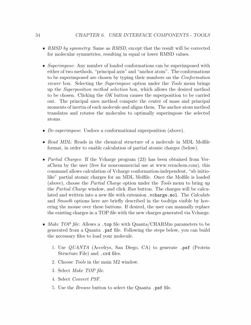
• Make TOP file: Allows a .top file with Quanta/CHARMm parameters to begenerated from a Quanta .psf file. Following the steps below, you can buildthe necessary files to load your molecule.

1. Use QUANTA (Accelrys, San Diego, CA) to generate .psf (ProteinStructure File) and .crd files.

2. Choose Tools in the main M2 window.

3. Select Make TOP file.

4. Select Convert PSF.

5. Use the Browse button to select the Quanta .psf file.

35

6. The .top file name should appear automatically in the same locationwith the same name as the .psf file, except with the .top extension.However, you may change the name or location here.

7. Press the Convert button. This will generate the files.

8. Select the Return to M2 button and you will have the corresponding TOPfile.

• TRJ → CRD: This allows a CHARMM format .crd file to be generated froma conformation displayed in the M2 graphics window.

• CRD → TRJ: Reverse of the previous option.

• Link files: Allows multiple .trj files to be linked into a single .trj file. Thiscan be useful, for example, when multiple Tork outputs need to be combinedinto a single .trj file for conformational filtering. Note that M2 does notallow multiple .trj files to be loaded at the same time, so linking them beforeloading is the only option. Save target file allows the user to specify the desiredname of the output .trj file. Then the File Selection Dialog allows the user tochoose the .trj files to be linked. Once the output .trj file has been written,it can be loaded with the Load button for further work.

• Export TRJ: Writes out a .trj file for the molecular conformations currentlydisplayed in the M2 graphics window.

• Clear window: Unload all molecules for a new calculation.

Chapter 7

M2 Files: Contents and Format

1. .psf - Protein structure file, a basic data file format used by the programCHARMM.

2. .top - M2 molecular topology file with the following contents:

• ATOM BLOCK: Atom index, CHARMM atom type, mass, charge (au),Lennard-Jones parameters (kcal/mol and A), and alternate Lennard-Jones parameters for 1-4 interactions.

• BOND BLOCK: Indices of the bonded atoms, force constant (kcal/mol/A),and equilibrium bond-length (A).

• ANGLE BLOCK: Indices of the atoms forming each angle, force constant(kcal/mol/radian2), and equilibrium value of the harmonic angle term.

• PROPER DIHEDRALS: Indices of the atoms forming the dihedral angle,the coefficient of the sinusoidal torsional energy term (kcal/mol), themultiplicity of the torsion, and phase of the torsion (radians).

• IMPROPER DIHEDRALS: Indices of the atoms forming the dihedral an-gle, the harmonic force constant (kcal/mol/radian2), and the equilibriumvalue of the angle.

• NBFIX BLOCK: Special Lennard-Jones parameters (kcal/mol A), whichoverride the standard combination rules for the specified atom-type pairs.

• NFINAL: numbers of atoms, bonds, angles, proper dihedrals and im-proper dihedrals. (The final integer can be ignored.)

3. .crd - CHARMM coordinate file

4. .trj - M2 trajectory file, which holds Cartesian coordinates of the outputconformations in a stacked PDB format. (For further information on thisformat, please see the source code that generates it, wtrjlm new.f.

36

37

5. .inp - An input file written by the GUI for one of the M2 executables. Thelines should be reasonable self-explanatory, based on the parameters visible inthe GUI windows and discussed in this manual.

6. .out - An output file from one of the M2 steps. The final output file (*-new-final.out)contains the chemical potential (free energy) and energy components for allthe filtered and sorted conformations, along with the corresponding cumulativeresults.

Chapter 8

Compilation and Automation

The source code for M2 1win.exe and M2 2win.exe is provided in the files M2 1.zip

and M2 2.zip, respectively. The code is written in FORTRAN 90 and was devel-oped and compiled on Windows XP with Compaq Visual Fortran. We have alsosuccessfully compiled both executables with the Intel(R) Fortran compiler underthe Windows XP and Linux operating systems. The IntelWindows and VisualFor-tranWindows folders contain the source code and workspaces for the correspondingcompilers. (You may need to modify the paths in the workspaces to match yourusage in order to use these.) The following notes provide additional information forcompiling and running the M2 codes.

• If you work on a large system, you may need to increase the sizes of somearrays. This can be done by modifying the file parameters.inc:

+ maxatm: maximum number of atoms.

+ maxbnd: maximum number of bonds.

+ maxang: maximum number of angles.

+ maxdih: maximum number of dihedrals.

+ maxnb: maximum size of the nonbonded pairlist

• The default compilation settings only need to be supplemented with the flags/fpp (to enable preprocessing) and /stack:0x1dcd6500 (to increase the stacksize).

• To port the code to the Linux environment and compile with the Intel ifortcompiler:

38

39

+ Place all the source code files provided in the VisualFortranWindows (sic)folder in a single directory on the Linux system, along with the providedMakefile.

+ Type “make all” at the Linux prompt to build the program.

+ M2 1.exe and M2 2.exe should be run at the command prompt with thenames of the desired input and output files on the command line; e.g.,“M2 1.exe B5 tork-tork.inp B5 tork-tork.out”.

+ You may use the input files generated with the Windows GUI as modelsfor your Linux runs.

• The Scripts folder provided with this distribution includes a collection of an-cillary scripts that automate the process of iterating the Tork/free energycalculation cycle to convergence. Please refer to the ReadMe file in the Scriptsfolder for information.

Chapter 9

Tips and Troubleshooting

• If the graphics window does not display a molecular system when you firstload it, use the right mouse button to rescale the display and the molecule(s)should show up.

• Starting with a poor conformation can lead to trouble. In particular, make surethat the initial bound conformation of your complex looks basically reasonable.Be aware that a conformation can be energy minimized to a local energyminimum yet be incorrect due, for example, to damaged stereochemistry, acovalent bond thrust through a phenyl ring, a ligand outside the receptor, etc.

• Tork is an aggressive search algorithm and sometimes generates abnormal con-formations, especially of macrocyclic hosts. Be sure to view the conformationsbefore computing the free energy. If there are abnormal conformations, youcan simply use a text editor to excise them from the .trj file to be used inthe free energy calculations.

• If the Tork calculations for the bound complex generate conformations withthe guest outside the binding site, it is usually a good idea to delete theseconformations before proceeding.

• Be aware that the free energy results depend upon the force field you use.Whereas the force field parameters for amino acids have been pretty highlyoptimized over the years, this is not the case for the varied atom types thatappear in host-guest chemistry. If your results are unsatisfactory, it is a goodidea to take a critical look at the force field parameters, or try using a differentset.

• Especially when working with a new system, it is a good idea to get a sensefor the convergence by doing several Tork runs with different random number

40

41

seeds.

• The present default parameters are based on our experiences with the M2software, but it is not a bad idea to experiment with variations, if only to geta sense for what they all do.

• Occasionally, Tork will not fully energy-minimize a conformation. In this case,the Mode Scan that occurs during the HA/MS free energy calculation mayscan into a lower-energy conformation. The way this plays out in the mathis that the conformation in question will be reported to have an abnormallylarge (favorable) entropy. Therefore, if you come across a conformation witha surprisingly large entropy, it is a good idea to try re-minimizing the energyand recalculating its free energy, just to be sure it is all right. The code doestry to catch these problems in advance: if the energy decreases more than“mintest” during Mode Scanning (Section 5.5), the scan is terminated and awarning message is written to the console.

• The version of UHBD that we adapted for M2 automatically scales the finitedifference grid to fit the molecule or complex you are studying. However, ifyour system is too large, the finite difference grid spacing may become toocoarse to yield good PB results. (A grid spacing of 0.3 Angstroms or smalleris best.) It is a good idea to check * fe-pb.out to make sure that UHBD isusing a sufficiently fine grid.

• When comparing with experiment, always take a careful look at the experi-mental methods to make sure they are appropriate and that you match themas closely as possible. For example, if the experiments use cyclodextrins athigh concentration, then the binding measurements may reflect not only 1:1host-guest binding, but also the formation of higher-order complexes, such asa 2:1 cyclodextrin:guest complex. Or, if the solvent is a mixture of water andmethanol, it may be hard to settle on appropriate solvation parameters for usein M2.

• In order to avoid file-format problems, it is safest to generate all input files viathe M2 GUI. You can use a text editor to revise them, but be sure to maintainan identical format.

• Remember to add the contribution of −RT ln(

8π2

C◦

)= 7.03 kcal/mol to the

computed binding free energy. See Equation 2.2 and Section 4.1.

• Filtering may crash when there is a large number of conformations. If thishappens, divide the trj file into several separate trj files with fewer conforma-tions, filter them separately, merge the filtered files, and then filter the mergedfile to get the final filtered trj file.

42 CHAPTER 9. TIPS AND TROUBLESHOOTING

• Remember that the present conformational filtering program will fail if anatom has more than 8 bonds. This can happen in the case of some metalloor-ganic complexes. You have the option of using a third-party filtering programand then loading the filtered conformations back into M2 for the free energycalculations.

• CRD and TOP files should follow the same format as the CRD and TOP filesin the Sample folder. Neither of the files should contain any header title atthe beginning or any other comment in between or at the end of the files.

• It is important that the pathnames associated with the M2 repository or anyof your working directories do not contain any blank space character or be toolong.

• When you generate a TOP file using the “Make TOP File” option under theTools menu, check that all the parameters are defined and your TOP file doesnot include any “n/a” flags. This flag, if present, means that a parameterrequired by the PSF file is not present in the parameter data files. You willneed to provide such parameters yourself by manually editing the TOP file.For example, the “ NX CT NX” angle set is not defined in our CB-original.topfile (see Sample folder) and a reasonable value has been manually inserted inCB.top.

Bibliography

[1] Gilson, M. K. Prot. Struct. Func. Gen., 1993, 15, 266–282.

[2] Gilson, M. K.; Given, J. A.; Head, M. S. Chem. & Biol., 1997, 4, 87–92.

[3] Chang, C.-E.; Potter, M. J.; Gilson, M. K. J. Phys. Chem. B, 2003, 107,1048–1055.

[4] Chang, C.-E.; Gilson, M. K. J. Comput. Chem., 2003, 24, 1987–1998.

[5] Chen, W.; Huang, J.; Gilson, M. K. J. Chem. Inf. Comput. Sci., 2004, 44,1301–1313.

[6] Kolossvary, I. J. Phys. Chem. A, 1997, 101, 9900–9905.

[7] Chang, C.-E.; Chen, W.; Gilson, M. K. Proc. Natl. Acad. Sci. USA, 2007, 104,1534–1539.

[8] Head, M. S.; Given, J. A.; Gilson, M. K. J. Phys. Chem., 1997, 101, 1609–1618.

[9] Polar hydrogen parameter set for CHARMm, Molecular Simulations Inc.Waltham, MA.

[10] Brooks, B. R.; Bruccoleri, R. E.; Olafson, B. D.; States, D. J.; Swaminathan,S.; Karplus, M. J. Comput. Chem., 1983, 4, 187–217.

[11] MacKerell, A.; Bashford, D.; Bellott, M.; Dunbrack, R.; Evanseck, J.; Field,M.; Fischer, S.; Gao, J.; Guo, H.; Ha, S.; Joseph-McCarthy, D.; Kuchnir, L.;Kuczera, K.; Lau, F.; Mattos, C.; Michnick, S.; Ngo, T.; Nguyen, D.; Prodhom,B.; Reiher, W.; Roux, B.; Schlenkrich, M.; Smith, J.; Stote, R.; Straub, J.;Watanabe, M.; Wiorkiewicz-Kuczera, J.; Yin, D.; Karplus, M. J. Phys. Chem.B, 1998, 102, 3586–3616.

[12] MacKerell, A. D. Jr.; Wiokiewicz-Kuczera, J.; Karplus, M. J. Am. Chem. Soc.,1995, 117, 11946–11975.

43

44 BIBLIOGRAPHY

[13] Weiner, S. J.; Kollman, P. A.; Case, D. A.; Singh, U. C.; Ghio, C.; Alagona,G.; Profeta, S.; Weiner, P. J. Am. Chem. Soc., 1984, 106, 765–784.

[14] Cornell, W. D.; Cieplak, P.; Bayly, C. I.; Kollman, P. A. J. Am. Chem. Soc.,1993, 115, 9620–9631.

[15] Gilson, M. K.; Honig, B. J. Comput. Aided. Mol. Des., 1991, 5, 5–20.

[16] Qiu, D.; Shenkin, P. S.; Hollinger, F. P.; Still, W. C. J. Phys. Chem., 1997,101, 3005–3014.

[17] Gilson, M. K.; Honig, B. Prot. Struct. Func. Gen., 1988, 4, 7–18.

[18] Sitkoff, D.; Sharp, K. A.; Honig, B. J. Phys. Chem., 1994, 98, 1978–1988.

[19] Chang, C.-E.; Gilson, M. K. J. Am. Chem. Soc., 2004, 126, 13156–13164.

[20] Davis, M. E.; Madura, J. D.; Luty, B. A.; McCammon, J. A. Comput. Phys.Commun., 1991, 62, 187–197.

[21] Zhou, H.; Gilson, M. K. Chem. Rev., 2009, Articles ASAP July 9, 2009.

[22] Chen, W.; Huang, J.; Gilson, M. K. J. Chem. Inf. Sci., 2004, 44, 1301–1313.

[23] Gilson, M. K.; Gilson, H. S. R.; Potter, M. J. J. Chem. Inf. Comput. Sci.,2003, 43, 1982–1997.