USER’S GUIDE TO MODEL VIEWER, A PROGRAM FOR THREE-DIMENSIONAL VISUALIZATION OF GROUND-WATER MODEL RESULTS

Open-File Report 02-106

U.S. Department of the InteriorU.S. Geological Survey

USER’S GUIDE TO MODEL VIEWER, A PROGRAM FOR THREE-DIMENSIONAL VISUALIZATION OF GROUND-WATER MODEL RESULTS

By Paul A. Hsieh and Richard B. Winston

U.S. GEOLOGICAL SURVEY

Open File Report 02-106

Menlo Park, California2002

U.S. DEPARTMENT OF THE INTERIORGALE A. NORTON, Secretary

U.S. GEOLOGICAL SURVEYCharles G. Groat, Director

The use of trade, product, industry, or firm names is for descriptive purposes only and does not imply endorsement by the U.S. Government.

For additional information write to:

Chief, Branch of Regional ResearchU.S. Geological Survey345 Middlefield Road, MS 472Menlo Park, CA 94025

CONTENTS

Abstract .................................................................................................................................... 1

Introduction.............................................................................................................................. 1Purpose and Scope ............................................................................................................. 1Computer Requirements .................................................................................................... 2Model Data Requirements ................................................................................................. 2Acknowledgments ............................................................................................................. 2

General Strategy for Three-dimensional Visualization............................................................ 2Scalar Data ......................................................................................................................... 3

Color Bar...................................................................................................................... 3Solid Representation .................................................................................................... 4Isosurface Representation ............................................................................................ 5Thresholding ................................................................................................................ 6Cropping ...................................................................................................................... 7

Vector Data ........................................................................................................................ 8Pathlines............................................................................................................................. 9Model Features and Auxiliary Graphic Objects .............................................................. 10

Zooming, Rotation, and Panning ............................................................................................11

User Interface......................................................................................................................... 12“File” Menu ..................................................................................................................... 12“Show” Menu .................................................................................................................. 14“Action” Menu................................................................................................................. 14“Toolbox” Menu .............................................................................................................. 15“Help” Menu.................................................................................................................... 18

References.............................................................................................................................. 18

iii

FIGURES

Figure 1. (a) Linear color bar. (b) Logarithmic color bar......................................................... 3

Figure 2. Solid representation using (a) “blocky” coloring scheme, (b) “smooth” coloring scheme, (c) “banded” coloring scheme............................................................................................ 4

Figure 3. Display of scalar data as a set of isosurfaces............................................................ 5

Figure 4. Thresholding a solid that is displayed in (a) blocky coloring scheme, (b) smooth coloring scheme, and (c) banded coloring scheme. ........................................................... 6

Figure 5. Use of the pair of y cropping planes at normalized coordinate of 0.3 and 0.7 as measured along the bounding box edge that is parallel to the y axis. ................................................ 7

Figure 6. Vectors in the top layer of a model grid. Small cubes indicate the starting points of the vector. The vector length is proportional to the vector magnitude. ................................... 8

Figure 7. Pathlines displayed as (a) lines and (b) narrow tubes. Color along pathlines indicates travel time, with blue indicating early time and red indicating late time. ......................... 9

Figure 8. Examples of auxiliary graphic objects displayed by Model Viewer. The x-y-z axes are respectively indicated by red, green and blue. The purple cells indicate cells containing wells. The gray cells are cells of specified head. ....................................................................... 10

Figure 9. The Model Viewer program window, showing menus and commands.................. 12

iv

User’s Guide To Model Viewer, A Program For Three-Dimensional Visualization Of Ground-water Model Results

By Paul A. Hsieh and Richard B. Winston

ABSTRACT

Model Viewer is a computer program that displays the results of three-dimensional ground-water models. Scalar data (such as hydraulic head or solute concentration) may be displayed as a solid or a set of isosurfaces, using a red-to-blue color spectrum to represent a range of scalar values. Vector data (such as velocity or specific discharge) are represented by lines oriented to the vector direction and scaled to the vector magnitude. Model Viewer can also display pathlines, cells or nodes that represent model features such as streams and wells, and auxiliary graphic objects such as grid lines and coordinate axes. Users may crop the model grid in different orientations to examine the interior structure of the data. For transient simulations, Model Viewer can animate the time evolution of the simulated quantities. The current version (1.0) of Model Viewer runs on Microsoft Windows 95, 98, NT and 2000 operating systems, and supports the following models: MODFLOW-2000, MODFLOW-2000 with the Ground-Water Transport Process, MODFLOW-96, MOC3D (Version 3.5), MODPATH, MT3DMS, and SUTRA (Version 2D3D.1). Model Viewer is designed to directly read input and output files from these models, thus minimizing the need for additional postprocessing. This report provides an overview of Model Viewer. Complete instructions on how to use the software are provided in the on-line help pages.

INTRODUCTION

A requirement for efficient use of numerical models is the ability of the modeler to visualize model results. This requirement is particularly important for three-dimensional ground-water models, which may involve complex geologic structures and tortuous pathlines. To meet this need, the computer program Model Viewer was developed to display the results of three-dimensional ground-water models.

Purpose and Scope

This report provides an overview of Model Viewer. Complete instructions on how to use the software can be found in the on-line help pages. The current version (1.0) of Model Viewer supports the following models: MODFLOW-2000 (Harbaugh and others, 2000), MODFLOW-2000 with the Ground-Water Transport Process (see Konikow and others, 1996, and update notes in program distribution package), MODFLOW 96 (Harbaugh and McDonald, 1996), MOC3D version 3.5 (Konikow and others, 1996), MODPATH (Pollock, 1994), MT3DMS (Zheng and Wang, 1999; Zheng and others, 2001), and SUTRA version 2D3D.1 (see Voss, 1984, and update notes in program distribution package). Model Viewer is designed to directly read input and output files of these models, thus minimizing the need for additional postprocessing.

1

Computer Requirements

Model Viewer is designed to run on the Microsoft Windows 95, 98, NT, and 2000 operating systems. The computer hardware requirements are as follows:• A minimum processor speed of 300 Megahertz. • A minimum of 64 Megabytes of Random Access Memory (RAM). Memory requirement

depends on the model size. A large model may require several hundred Megabytes.• A monitor with at least 16-bit color depth. 24-bit color is recommended.• The responsiveness of the program to user interaction increases with the speed of the graphics

board. A graphics board with OpenGL acceleration is highly recommended.• The program requires 9 Megabytes of hard disk space.

Model Data Requirements

Before using Model Viewer, the user must first run a model to generate simulation results. Model input files should be prepared according to instructions in the model documentation or user's guide. However, a few additional requirements are necessary to visualize results in Model Viewer. The additional requirements, and the procedure for loading model data files, vary from one model to another. Complete details are given in the on-line help pages. As a general rule, Model Viewer should be used only after a model run has been successfully executed. After the model data are successfully loaded, the methods described in this report can be used to explore the model data.

Acknowledgments

The authors are grateful to Will Schroeder, Ken Martin, and Bill Lorensen for creating the Visualization ToolKit (VTK), without which Model Viewer could not have been developed. VTK is an open source, freely available software system for three-dimensional computer graphics, image processing, and visualization (Schroeder and others, 1997). The authors of VTK has granted permission to use, copy, and distribute VTK while retaining their copyright.

GENERAL STRATEGY FOR THREE-DIMENSIONAL VISUALIZATION

Model Viewer displays three types of model simulation results: scalar data (such as hydraulic head or solute concentration), vector data (such as fluid velocity or specific discharge), and pathlines. In addition, Model Viewer displays cells or nodes that represent model features (such as streams, wells, or boundary conditions) and auxiliary graphic objects (such as grid lines, coordinate axes, and bounding box).

Because Model Viewer supports multiple models, differences in terminology might cause confusion in a general discussion. For example, the terms “grid” and “cell” are typically associated with finite-difference models, whereas the analogous terms “mesh” and “element” are typically associated with finite-element models. For the sake of uniformity in this report, the term

2

“grid” is understood to mean “mesh” when the discussion applies to finite-element models. Similarly, the term “cell” is understood to mean “element.”

For all models supported by Model Viewer, scalar data are computed at the nodes of the model grid. However, the position of a node within the grid depends on the particular model. For example, in a finite-difference model (such as MODFLOW), nodes are positioned at cell centers. By contrast, in a finite-element model (such as SUTRA), nodes are positioned at cell (element) vertices. The difference in node location affects certain display options, which may be available for finite-difference models but not for finite-element models, and vice versa.

Scalar Data

The general approach to visualizing the three-dimensional distribution of scalar values is to use a color spectrum (called a color bar) to represent a range of scalar values. The scalar data may be displayed as a solid or a set of isosurfaces. The interior details of the scalar data may be explored by cropping and thresholding, which are discussed below.

Color Bar

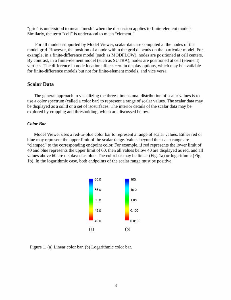
Model Viewer uses a red-to-blue color bar to represent a range of scalar values. Either red or blue may represent the upper limit of the scalar range. Values beyond the scalar range are “clamped” to the corresponding endpoint color. For example, if red represents the lower limit of 40 and blue represents the upper limit of 60, then all values below 40 are displayed as red, and all values above 60 are displayed as blue. The color bar may be linear (Fig. 1a) or logarithmic (Fig. 1b). In the logarithmic case, both endpoints of the scalar range must be positive.

Figure 1. (a) Linear color bar. (b) Logarithmic color bar.

(a) (b)

3

Solid Representation

In solid representation, all active cells in the grid are colored by mapping nodal values to the color bar. Inactive cells, if present in the grid, are excluded. Because the solid is rendered as opaque, only the exterior surface is visible. The interior of the solid can be examined by two methods: thresholding and cropping. These methods are discussed below.

Model Viewer provides three coloring schemes for solid representation. In the “blocky” coloring scheme, each cell has a uniform color according to the nodal value for that cell (Fig. 2a). The “blocky” coloring scheme is available only for finite-difference models (such as MODFLOW) but not for finite-element models (such as SUTRA). In the “smooth” coloring scheme, nodal values are interpolated to yield scalar values that vary smoothly from one node to another. Consequently, the colors vary smoothly through the solid (Fig. 2b). In the “banded” coloring scheme, solid is divided by isosurfaces into a discrete number of bands. Each band has a uniform color (Fig. 2c).

Figure 2. Solid representation using (a) “blocky” coloring scheme, (b) “smooth” coloring scheme, (c) “banded” coloring scheme.

(a) (b)

(c)

4

Isosurface Representation

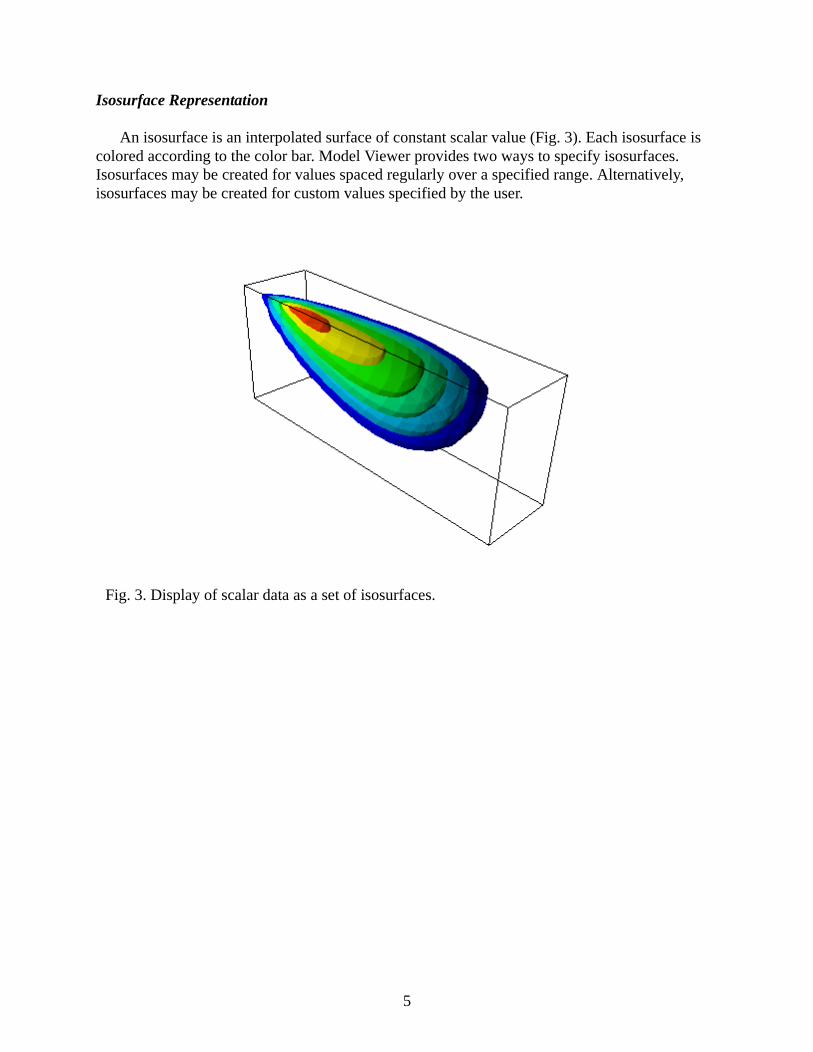
An isosurface is an interpolated surface of constant scalar value (Fig. 3). Each isosurface is colored according to the color bar. Model Viewer provides two ways to specify isosurfaces. Isosurfaces may be created for values spaced regularly over a specified range. Alternatively, isosurfaces may be created for custom values specified by the user.

Fig. 3. Display of scalar data as a set of isosurfaces.

5

Thresholding

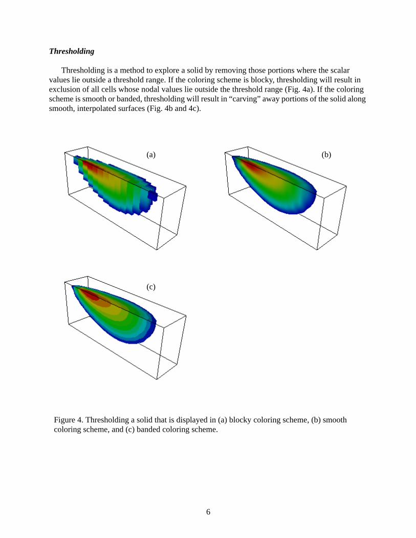
Thresholding is a method to explore a solid by removing those portions where the scalar values lie outside a threshold range. If the coloring scheme is blocky, thresholding will result in exclusion of all cells whose nodal values lie outside the threshold range (Fig. 4a). If the coloring scheme is smooth or banded, thresholding will result in “carving” away portions of the solid along smooth, interpolated surfaces (Fig. 4b and 4c).

Figure 4. Thresholding a solid that is displayed in (a) blocky coloring scheme, (b) smooth coloring scheme, and (c) banded coloring scheme.

(a) (b)

(c)

6

Cropping

Cropping is a method for exploring a solid or a set of isosurfaces by showing only the portion that lies on one side of a cropping plane. Model Viewer implements three pairs of cropping planes, denoted as the x, y, and z cropping planes. By default, the pair of x cropping planes is perpendicular to the x axis, and similarly for the y and z cropping planes. However, the x and y cropping planes may also be rotated. When cropping is enabled, only that portion of the solid between a pair of cropping planes is displayed.

The location of a cropping plane is defined by the normalized coordinate along the edge of the bounding box, which encloses the grid and is aligned with the x-y-z coordinate axes. The normalized coordinate is 0 at one terminus of the edge and 1 at the other terminus. For example, Fig. 5 illustrates the use of the y cropping planes at normalized coordinate of 0.3 and 0.7.

Figure 5. Use of the pair of y cropping planes at normalized coordinate of 0.3 and 0.7 as measured along the bounding box edge that is parallel to the y axis.

xy

z0.3

0.7

0

1

y cropping planebounding

box

7

Vector Data

Model Viewer displays a vector as a line oriented in the direction of the vector (Fig. 6). The length of the vector is proportional to the vector magnitude. The starting point of the vector is the node at which the vector is defined. A small cube (called the “base”) may be displayed at the starting point. Showing all vectors in the grid may result in a very cluttered picture. To avoid this, vectors can be displayed for a selected range of i, j, and k indices of the grid. In addition, the vector data may be “subsampled” by showing every n-th vector (n > 1) along the i, j, and k directions. Thresholding may be applied to display only those vectors having magnitudes in a specified range.

Figure 6. Vectors in the top layer of a model grid. Small cubes indicate the starting points of the vector. The vector length is proportional to the vector magnitude.

8

Pathlines

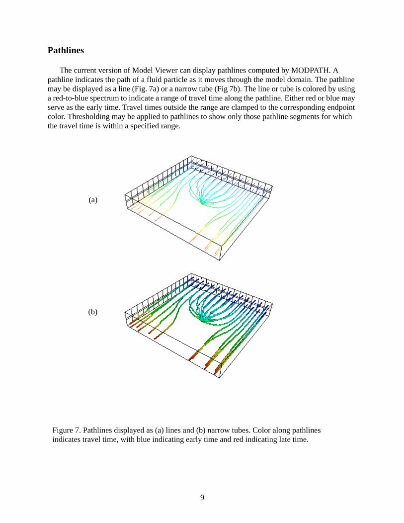
The current version of Model Viewer can display pathlines computed by MODPATH. A pathline indicates the path of a fluid particle as it moves through the model domain. The pathline may be displayed as a line (Fig. 7a) or a narrow tube (Fig 7b). The line or tube is colored by using a red-to-blue spectrum to indicate a range of travel time along the pathline. Either red or blue may serve as the early time. Travel times outside the range are clamped to the corresponding endpoint color. Thresholding may be applied to pathlines to show only those pathline segments for which the travel time is within a specified range.

Figure 7. Pathlines displayed as (a) lines and (b) narrow tubes. Color along pathlines indicates travel time, with blue indicating early time and red indicating late time.

(a)

(b)

9

Model Features and Auxiliary Graphic Objects

For finite-difference models, Model Viewer can also display cells that represent model features such as streams, wells, or boundary conditions. For finite-element models, model features are indicated by small colored cubes at appropriate nodes. Model Viewer can also display a number of auxiliary graphic objects to provide spatial reference and orientation. These objects include: a bounding box, grid lines, an axes symbol indicating the orientation of the x-y-z axis system, and a transparent “shell” indicating the outer surface of the active grid. Fig. 8 illustrates these auxiliary graphic objects.

Figure 8. Examples of auxiliary graphic objects displayed by Model Viewer. The x-y-z axes are respectively indicated by red, green and blue. The purple cells indicate cells containing wells. The gray cells are cells of specified head.

bounding box grid shell

axes

grid line

symbol

10

ZOOMING, ROTATION, AND PANNING

Model Viewer displays an object as viewed from a particular viewpoint. Zooming, rotation, and panning are different ways to interact with the object by changing the viewpoint:• Zooming in moves the viewpoint closer to the object being viewed, causing the object to appear

bigger.• Zooming out moves the viewpoint away from the object being viewed, causing the object to

appear smaller.• Rotation moves the viewpoint in an angular direction so that the viewed object appears to rotate.• Panning moves the viewpoint laterally so that the viewed object appears to move sideways.

Zooming, rotation, and panning are performed using the mouse. Two types of mouse interactions are provided: trackball-mode interaction, and joystick-mode interaction. Trackball-mode interaction is the default. However, the user may change the mouse interaction from one mode to another, using the Preferences command under the File menu (see section on “User Interface”).

The trackball-mode interaction works as follows. First, the cursor must be inside the program window. Then:• To zoom in, press and hold the right mouse button, and drag the cursor upward.• To zoom out, press and hold the right mouse button, and drag the cursor downward.• To rotate, press and hold the left mouse button, and drag the cursor in the direction of rotation.• To rotate around an axis perpendicular to the screen, hold down the Ctrl key, press and hold the

left mouse button, and drag the cursor in the direction of rotation. • To pan, hold down the Shift key, press and hold the left mouse button, and drag the cursor in the

direction of panning.

In joystick-mode interaction, the speed and direction of zooming, rotation, and panning are determined by the position of the cursor relative to the center of the program window. When the cursor is far from the center of the window, interaction is faster. When the cursor is near the center of the window, interaction is slower. Joystick-mode interaction works as follows:• To zoom in, place the cursor on the upper half of the window, and hold down the right mouse

button. To end zooming, release the button.• To zoom out, place the cursor on the lower half of the window, then press and hold the right

mouse button. To end zooming, release the button.• To rotate, place the cursor such that its position relative to the window center indicates the

direction of rotation, then press and hold the left mouse button. To end rotation, release the button.

• To rotate around an axis perpendicular to the screen, place the cursor such that its position relative to the window center indicates the direction of rotation, then press and hold the Ctrl key and left mouse button. To end rotation, release the button.

• To pan, place the cursor such that its position relative to the window center indicates the direction of panning, hold down the Shift key, then press and hold the left mouse button. To end panning, release the button.

11

USER INTERFACE

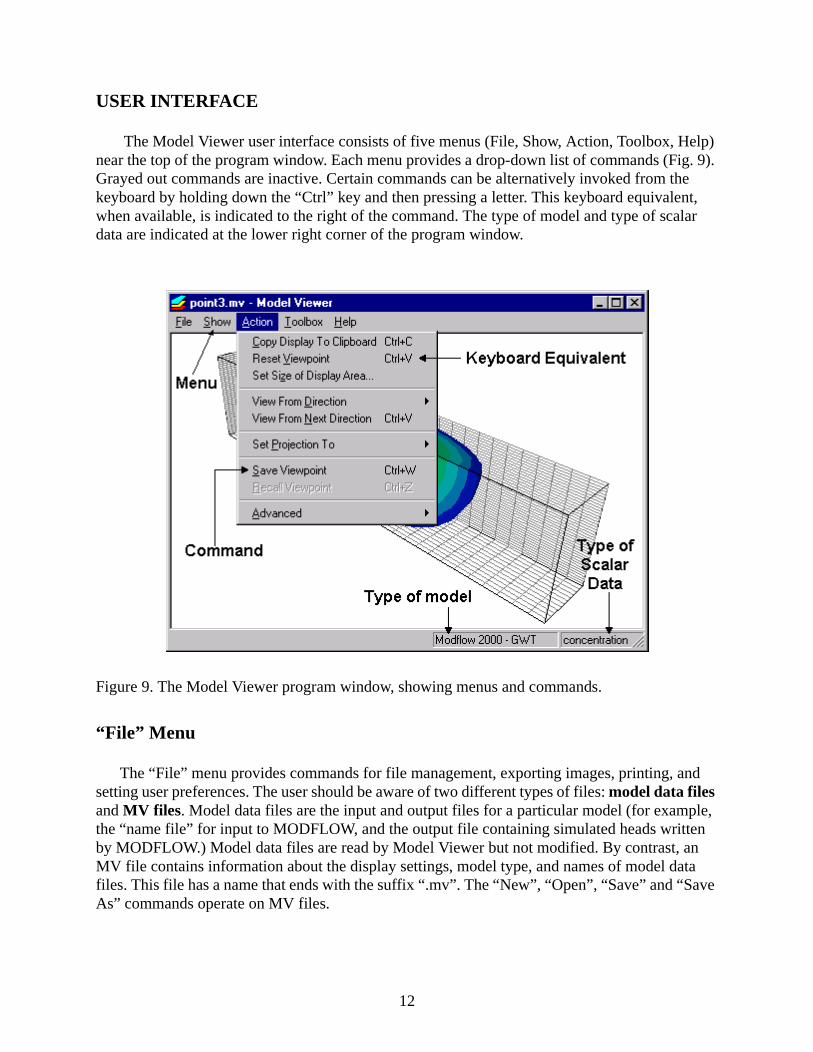
The Model Viewer user interface consists of five menus (File, Show, Action, Toolbox, Help) near the top of the program window. Each menu provides a drop-down list of commands (Fig. 9). Grayed out commands are inactive. Certain commands can be alternatively invoked from the keyboard by holding down the “Ctrl” key and then pressing a letter. This keyboard equivalent, when available, is indicated to the right of the command. The type of model and type of scalar data are indicated at the lower right corner of the program window.

Figure 9. The Model Viewer program window, showing menus and commands.

“File” Menu

The “File” menu provides commands for file management, exporting images, printing, and setting user preferences. The user should be aware of two different types of files: model data files and MV files. Model data files are the input and output files for a particular model (for example, the “name file” for input to MODFLOW, and the output file containing simulated heads written by MODFLOW.) Model data files are read by Model Viewer but not modified. By contrast, an MV file contains information about the display settings, model type, and names of model data files. This file has a name that ends with the suffix “.mv”. The “New”, “Open”, “Save” and “Save As” commands operate on MV files.

12

Every time the user changes a display setting (for example, the color bar limits), the current MV file is considered to have been changed. If the MV file was not saved after the changes, and the user tries to (a) create a new MV file, or (b) close the current MV file, or (c) exit Model Viewer, the user will be prompted to save the MV file before continuing.

The “New” command begins the process of creating a new MV file. A “Model Selection” dialog box is displayed for the user to select the type of model. Next, a “Data File” dialog box is displayed for the user to specify model data files. The procedure for loading data depends on the selected model and is given in the on-line help pages.

The “Open” command displays a dialog box for the user to specify the MV file to open. Because the MV file contains the names of model data files, Model Viewer will read data from these files. The data are then displayed using the settings saved in the MV file.

The “Close” command closes the current display of data. The program window becomes blank. The Close command is useful during repeated cycles of running a model and viewing the results. While model results are being displayed in Model Viewer, those model data files cannot be over-written by another program. Invoking the Close command releases the model data files so that the model can run to generate a new set of results.

The “Save” command saves the current display settings (for example, number of isosurfaces) to the current MV file. If the MV file was newly created, a dialog box is displayed for the user the specify the name of the MV file.

The “Save As” command saves the current display settings to an MV file of a different name.

The “Export as Bmp” commands exports the current display (in the program window) to a Windows bitmap file having a color depth of 24 bits per pixel or a maximum of about 16 million colors. A dialog box is displayed for resolution and size specification. Selecting “screen” resolution will export a bitmap image that is suitable for screen display. Selecting 150 or 300 ppi (pixels per inch) will generate a higher resolution bitmap image suitable for printing. For these two options, the user must specify either the width or the height (in inches) of the bitmap image. If the user specifies the width, then the height will be automatically determined so that the aspect ratio of the bitmap matches that of the window. If the user specifies the height, then the width will be automatically determined. For example, if the user specifies 300 ppi and a width of 4 inches, the bitmap will have 1200 pixels in the x dimension. When such a bitmap is imported into an application that recognizes bitmap resolution, the bitmap will be displayed as a picture with the specified width and height in inches.

The “Export as VRML” command exports a current display to a file containing VRML (Virtual Reality Modeling Language) data. A dialog box is displayed for the user to specify the file name, which should terminate with the suffix “.wrl”. A VRML file may be opened and viewed in a VRML viewing application.

The “Export Animation” command exports a sequence of Windows bitmap files, one for each time when model results are saved. These files may be used to create an animation (for

13

example, mpg, animated gif) using an application that creates animations. A dialog box is displayed for the user to specify the starting and ending times, the amount by which the viewpoint is rotated and/or elevated between successive times, and the naming convention for the bitmap files. The naming convention consists of a “file prefix” and a “start number”. For example, if the file prefix is sim and the start number is 001, then files will be named sim001.bmp, sim002.bmp, sim003.bmp, and so on. The “Preview” button displays the sequence of images to be exported without actually writing the files. The “Export” button begins the exporting process. Note that the bitmap files are not compressed and might occupy a significant amount of disk space. To conserve disk space, resize the window to a relatively small size before exporting.

The “Print” command prints the current display to a single page on a printer. The display is always scaled so that it will fit on one page. The printed page may be previewed with the “Print Preview” command. Printing options (for example, portrait versus landscape orientation) can be specified with the “Print Setup” command.

The “Preferences” command displays a dialog box for the user to set preferences. The current version of Model Viewer allows the user to set the mouse interaction to either “trackball mode” or “joystick mode.” These modes are explained in the section “Rotation, Zooming, and Panning.”

The “Exit” command terminates the Model Viewer program.

“Show” Menu

The “Show” menu provides commands to show or hide different types of graphic objects. The first three commands (Solid, Isosurface, None) respectively control the display of scalar data. The user may select one of the three command to display a solid, a set of isosurfaces, or to hide the scalar data. The remaining nine commands (Vectors, Pathlines, Model Features, Grid Shell, Grid Lines, Axes Symbol, Bounding box, Time, and Color Bar) alternately show and hide the corresponding graphic objects. A check mark next to a command indicates that the corresponding graphic object is shown. Selecting this command will hide the graphic object. The absence of a check mark next to a command indicates that the corresponding graphic object is hidden. Selecting the command will toggle the check mark and thus either show or hide the graphic object.

“Action” Menu

The “Action” menu provides commands to control the overall aspects of the display, such as display size, view direction, projection mode.

The “Copy to Clipboard” command copies the current display into the computer’s clipboard. The clipboard content may be pasted to another application that accepts graphic images.

The “Reset Viewpoint” changes the viewpoint so that all visible graphic objects can be seen in the program window.

14

The “Set Display Size” command displays a dialog box for the user to set the display (the area inside the window frame) to a specific size (in pixels). This command is useful for exporting a bitmap of a specific size.

The “View From Direction” command sets the viewpoint so that the display is viewed from one of six preset directions provided by the sub-commands to the right. The sub-command “+x” means viewing from the positive x direction to the negative x direction. The sub-command “-x” means viewing from the negative x direction to the positive x direction. Analogous definitions apply to the sub-commands “+y”, “-y”, “+z” and “-z”.

The “View From Next Direction” command changes the viewpoint from one preset direction to another. The order of view directions are: +x, +y, -z, +z, -x, -y.

The “Set Projection to” commands sets the projection mode to “perspective” or “parallel”. In perspective mode, parallel lines appear to converge to a point at infinity. This is the default projection mode. In parallel mode, parallel lines appear to remain parallel to each other as they extend to infinity. Parallel projection is of limited usefulness in three-dimensional visualization, but can be used to align grid nodes or to compare vector lengths.

The “Save Viewpoint” command saves the current viewpoint. The saved viewpoint may be restored by using the “Restore Viewpoint” command. Note that the viewpoint is saved only temporarily and is discarded when the program terminates.

The “Advanced” command has a single sub-command “Assume All Active Cells”. If all cells in the model grid are active, invoking this command can speed up calculations required for graphical rendering. If the model grid contains inactive cells, this sub-command should not be invoked. Otherwise, inactive cells will not be excluded from the display.

“Toolbox” Menu

The “Toolbox” menu provides commands to show or hide small dialog boxes (called toolboxes) for controlling specific aspects of the display. A check mark next to a command indicates that the corresponding toolbox is shown. Selecting this command will hide the toolbox. The absence of a check mark next to a command indicates that the corresponding toolbox is hidden. Selecting this command will show the toolbox. Each toolbox may be closed by clicking the “Done” button. Note that toolboxes do not have to be closed for the program to continue. Except for text entries, all controls on toolboxes will take effect immediately when changed. For text entries, the user must click the "Apply" button to apply the change.

Certain toolboxes refer to the coordinate axis variables x, y, z, and grid index variables i, j, and k. The meaning of these variables depends on the model. For a finite-difference model, the x-y-z axis system is not explicitly defined. Model Viewer uses the following convention. The x axis and the index i run along a row. The y axis and the index j run along a column. The z axis is perpendicular to the x and y axes, and points upward. The index k runs along the z axis and typically indicates layers, with k = 1 indicating the bottom layer. (Note that this is opposite to the

15

MODFLOW convention where k = 1 indicates the top layer.) For a finite-element model, the x-y-z axis system and the i-j-k indexing scheme are the same as those defined in the model.

The “Data” toolbox contains three tab panels. The “Scalar” tab provides a drop-down list box for the user to select the type of scalar data to display, and also shows the maximum and minimum scalar value at the current time. The “Vector” tab shows the maximum and minimum vector magnitude in the current time. The “Pathline” tab shows the maximum and minimum travel time.

The “Color Bar” toolbox controls the properties of the color bar. The “Limits” tab provides text boxes to set the scalar values at the red and blue limits. The default color bar uses a linear scale, but a logarithmic scale can be used by checking the “logarithmic scale” option box. The “Reverse” button reverses the red and blue limits. The “Size” tab provides text boxes to set the color bar width and height (in pixels) and the offset from the right side of the window. The “Labels” tab provide text boxes to set the label font size, the number of labels, and numerical precision (number of significant digits). User may also set the font color as black, gray, or white. Clicking the “Default” button at the bottom of the toolbox sets default values to all options in the selected tab.

The “Lighting” toolbox allows fine adjustment of how the graphic objects are illuminated. The default lighting is a “headlight” illuminating the graphic objects from the direction of the viewpoint. This setting is usually adequate for most cases. However, for fine adjustments, the headlight intensity may be decreased or completely turned off (under the “Lights” tab). In addition, the user may turn on an “auxiliary light” for illumination from a direction specified by a vector whose x-y-z components may vary from -1 to 1. For example, if x=1, y=0, z=0, the auxiliary light will shine from the positive x axis towards the negative x axis. The “Surface” tab provides controls over the surface parameters of the graphic objects. These parameters include: • Diffuse: This parameters is currently not adjustable and is set to 1.0. • Ambient: Increasing this parameter above 0 gives surfaces a "washed out" appearance and

reduces the shading. Setting this parameter to the maximum value of 1 causes surfaces to appear white.

• Specular: The amount of reflected light,• Specular Power: The surface shininess.

The “Background” tab enables the user to specify the background color by setting the red, green, and blue components.

The “Grid” toolbox contains three tab panels. The “Lines” tab controls three sets of gridlines displayed respectively at the i, j, and k grid index positions. Each set of grid lines may be activated (shown) or inactivated (hidden). The user may also set the grid line color to black, gray, or white. The “Shell” tab controls the color and opacity of the grid shell (see Fig. 8). The “Subgrid” tab enables the user to show a subset of the grid as defined by minimum and maximum values for the i, j, and k indices.

The “Geometry” toolbox contains three tab panels. The “Scale” tab controls the exaggeration (or stretch) factor in the x, y and z directions. The “Axes Symbol” tab controls the size and position of the axes symbol. The “Bounding Box” tab controls the color of the bounding box.

16

The “Solid” toolbox enables the user to select the between the smooth, blocky, or banded coloring schemes. If the banded coloring scheme is selected, the number of color bands must be specified (between 2 and 50). The user may also apply thresholding by setting a maximum and minimum value.

The “Isosurface” toolbox contains two tab panels. The “Regular” tab enables the user to set a number of isosurfaces uniformly spaced between a maximum and a minimum value. The “Custom” tab enables the user to specify a custom value for each isosurface. To specify a custom value, enter the value in the text box on the left and click the “Add” button. To remove a custom value, select the value in the list box on the right and click the “Delete” button.

The “Vector” toolbox controls the display of vectors. The “Controls” tab enables the user to selectively display vectors by setting the range of i, j, and k indices. The vector data may be “subsampled” by setting the “rate” to be greater than 1. For example, if the minimum and maximum i indices are 3 and 20 and “rate” is set at 4, vectors will be displayed at i values of 3, 7, 11, 15 and 19. Under the “Appearance” tab, the user may increase or decrease the vector length by changing the scale factor. The user may also show or hide the vector bases, control their sizes, and specify the vector color. The “Threshold” tab enables the user to display only those vectors having magnitudes that fall within a specified range.

The “Pathlines” toolbox controls the display of pathlines. The “Appearance” tab provides the options to show the pathlines as lines or as tubes of specified diameter (in pixels). The “Color” tab provides text boxes to set the travel times at the red and blue endpoints. The “Threshold” tab provides three threshold options: no threshold: (complete pathlines are shown), threshold by simulation time (pathline segments are shown for travel times from the start of the simulation to the current time), and threshold by time range (pathline segments are shown for the specified travel time range).

The “Model Features” toolbox contains two lists--the “Show” list on the left and the “Hide” list on the right. Model features in the Show list are visible; those in the “Hide” list are invisible. To hide a model feature in the Show list, select the item and click the “Hide” button. To show an model feature in the Hide list, select the item and click the “Show” button. To change the color of a model feature, select the item and click the “Color” button. If several model features occupy the same cell or node, the uppermost item in the Show list will be displayed. The order of the Show list may be rearranged by clicking an item and then clicking the “Top”, “Up”, “Down” or “Bottom” button.

The “Crop” toolbox controls cropping a solid or a set of isosurfaces. As illustrated in Fig. 5, the cropping planes are defined by normalized coordinate along the x, y, and z edges of the bounding box. These normalized coordinates are entered into the boxes under “Min” and “Max” (under the “Controls” tab). Clicking the up or down arrowheads increases or decreases the Max or Min value by the amount in the “Delta” box. Checking the “Max = Min” option sets the Max value equal to the Min value to display a two-dimensional slice. The “Options” tab provides the option to display the outer shell of the cropped-away solid or the cropped-away isosurfaces. The four sliders can be used to set the color and opacity of the cropped-away pieces.

17

The “Animation” toolbox controls the display of model results at successive times. In the “Controls” tab, the “Advance” button advances to the next time. The “Run” button displays successive times until the end of the data set. To set the display to a particular time, select that time from the “Set to time” drop-list box, and then click “Set”. In the “Options” tab, the user may reduce the animation speed by introducing a delay (in seconds) between successive times. To animate at the fastest speed, enter 0 in the Delay box. The viewpoint can also be rotated (horizontally) or elevated (vertically) by a specified angular increment between successive times. For a stationary viewpoint during animation, enter 0 in the Rotate and Elevate boxes.

“Help” Menu

The help menu provides two commands. The “Contents” command displays the on-line help pages. The “About Model Viewer” command displays the program version number, notice to the user, disclaimer, and credits.

REFERENCES

Harbaugh, A.W., Banta, E.R., Hill, M.C., and McDonald, M.G., 2000, MODFLOW-2000, the U.S. Geological Survey modular ground-water model--user guide to modularization concepts and the ground-water flow process: U.S. Geological Survey Open-File Report 00-92, 121 p.

Harbaugh, A.W., and McDonald, M.G., 1996, User's documentation for MODFLOW-96, an update to the U.S. Geological Survey modular finite-difference ground-water flow model: U.S. Geological Survey Open-File Report 96-485, 56 p.

Konikow, L.F., Goode, D.J., and Hornberger, G.Z., 1996, A three-dimensional method-of-characteristics solute-transport model (MOC3D): U.S. Geological Survey Water-Resources Investigations Report 96-4267, 87 p.

Pollock, D.W., 1994, User's Guide for MODPATH/MODPATH-PLOT, Version 3: A particle tracking post-processing package for MODFLOW, the U.S. Geological Survey finite-difference ground-water flow model: U.S. Geological Survey Open-File Report 94-464, 6 ch.

Schroeder, Will, Martin, Ken, and Lorensen, Bill, 1997, The Visualization Toolkit: An Object-Oriented Approach to 3D Graphics, 2nd Edition: Upper Saddle River, New Jersey, Prentice Hall PTR, 672 p.

Voss, C.I., 1984, A finite-element simulation model for saturated-unsaturated, fluid-density-dependent ground-water flow with energy transport or chemically-reactive single-species solute transport: U.S. Geological Survey Water-Resources Investigations Report 84-4369, 409 p.

Zheng, Chunmiao, Hill, M.C., and Hsieh, P.A., 2001, MODFLOW-2000, the U.S. Geological Survey modular ground-water model--User guide to the LMT6 package, the linkage with MT3DMS for multi-species mass transport modeling: U.S. Geological Survey Open-File Report 01-82, 43 p.

Zheng, Chunmiao, and Wang, P.P., 1999, MT3DMS, A modular three-dimensional multi-species transport model for simulation of advection, dispersion and chemical reactions of contaminants in groundwater systems; documentation and user’s guide: U.S. Army Engineer Research and Development Center Contract Report SERDP-99-1, Vicksburg, MS, 202 p.

18