usgs · pdf fileshkied-ftiicf b«e frm 1:250.000^c»lc difal qevttoi modd; b...

Simulated Effects of Potential ^ Withdrawals from Wells Near , Yucca Mountain, Nevada

U.S. GEOLOGICAL SURVEY

Water-Resources Investigations Report 99-4166

Prepared in cooperation with the U.S. DEPARTMENT OF ENERGY

USGSscience for a changing world

Simulated Effects of Potential Withdrawals from Wells Near Yucca Mountain, Nevada

By Patrick Tucci and Claudia C. Faunt


Water-Resources Investigations Report 99-4166

Prepared in cooperation with theU.S. DEPARTMENT OF ENERGYunder Interagency Agreement DE-AI08-97NV12033

Denver, Colorado 1999

U.S. DEPARTMENT OF THE INTERIOR BRUCE BABBITT, Secretary


Charles G. Groat, Director

The use of firm, trade, and brand names in this report is for identification purposes only and does not constitute endorsement by the U.S. Geological Survey.

For additional information write to:

Chief, Earth Science Investigations ProgramYucca Mountain Project BranchU.S. Geological SurveyBox 25046, Mail Stop 421Denver Federal CenterDenver, CO 80225-0046

Copies of this report can be purchased from:

U.S. Geological Survey Information Services Box 25286 Federal Center Denver, CO 80225

CONTENTS

Abstract ......................................................................... 1Introduction ...............................................................................................................^^^ 1

Purpose and Scope I.................................................................................................................................................. 3Summary of Hydrogeologic Conditions................................................................................................................... 3Previous Modeb'ng .................................................................................i................................................................. 3Description of Wells J-12, M3,andUE-25c#3...................................................................................................... 5

Simulated Effects of Potential Withdrawals ......................................................................................................................... 6Description of the 1997 Regional Flow Model....................................................................................................... 6Modification to the 1997 Regional Flow Model ...................................................................................................... 8Baseline Simulation..........................................................................^ 8Simulation of Increased Withdrawals ...................................................................................................................... 10

Model Limitations and Discussion ....................................................................................................................................... 10Summary ..................................................................... 13References Cited .................................................................................................................................................................. 14

FIGURES

1-5. Maps showing:1. Location of regional flow-model boundary and selected hydrographic areas of the Death Valley region ............... 22. Location of selected wells and model grid cells near Yucca Mountain ................................................................... 43. Simulated potentiometric surface in 1997 regional flow model, upper layer, near Yucca Mountain....................... 74. Simulated water-level declines for the baseline simulation, upper model layer ...................................................... 95. Simulated water-level declines for the predictive simulation, upper model layer ...:............................................... 11

TABLES

1. Summary of average annual pumping rates for wells J-12 and J-13,1983-97......................................................... 52. Summary of model simulations................................................................................................................................ 8

CONVERSION FACTORS AND VERTICAL DATUM___________________________________

Multiply By To obtain

kilometer (km) 0.6214 milemeter (m) 3.2808 foot

square meter per day (m2/d) 10.7649 square foot per daysquare kilometer (km2) 0.3861 square mile

cubic meters per day (m3/d) 0.1835 gallon per minutecubic meters per day (m3/d) 0.2961 acre-foot per year (ac-ft/yr)

Sea level: In this report "sea level" refers to the National Geodetic Vertical Datum of 1929 (NGVD of 1929)~a geodetic datum derived from a general adjustment of the first-order level nets of both the United States and Canada, formerly called Sea Level Datum of 1929.

CONTENTS III

SIMULATED EFFECTS OF POTENTIAL WITHDRAWALS FROM WELLS NEAR YUCCA MOUNTAIN, NEVADABy Patrick Tucci and Ciaudia C. Faunt

Abstract

The effects of potential future withdrawals from wells J-12, J-13, and UE-25c #3 on the ground-water flow system in the area surrounding Yucca Mountain, Nevada, were simulated by using an existing (1997) three-dimensional regional ground-water flow model. The 1997 regional model was modified only to include changes at the pumped wells. Two steady-state simulations (baseline and predictive) were conducted to estimate changes in water level and changes in ground-water outflow from Jackass Flats, where the pumped wells are located, south to the Amargosa Desert.

The baseline simulation included 1983-97 average pumping from wells J-12 and J-13, which was not included in the 1997 regional flow model. Water levels at a site near the town of Amargosa Valley were 0.4 meters lower in the baseline simulation than the simulated levels for the 1997 model. Simulated water-level declines at model cells that contain the pumped wells were some what larger than those near Amargosa Valley, but the declines generally were less than 1 meter within a few kilometers of the pumped wells. Ground-water outflow from Jackass Flats to the Amargosa Desert in the baseline simulation was 200 cubic meters per day less than that of the 1997 regional model.

The predictive simulation included poten tial pumping at wells J-12, J-13, and UE-25c #3 at a rate of 569 cubic meters per day for each well, an increase of 1,090 cubic meters per day over the

total baseline simulation rates. Water levels at a site near the town of Amargosa Valley were 1.1 meters lower in the predictive simulation than the levels for the baseline simulation. Simulated water-level declines at model cells that contain the pumped wells were also somewhat larger than those near Amargosa Valley, but the declines generally were less than 2 meters within a few kilometers of the pumped wells. Ground-water outflow from Jackass Flats to the Amargosa Desert in the predictive simulation was 500 cubic meters per day less than that of the baseline simu lation.

Some small errors in the simulated effects of potential increased withdrawals are present in this analysis, particularly the simulated water- level changes estimated for the pumped wells and the immediate vicinity of those wells, due to numerical constraints, violations of model assumptions, possible differences in simulated and actual transmissivity values, and the coarse model discretization. The errors in simulated effects are probably somewhat less due to those causes at cells a few kilometers from the pumped wells, such as those near the town of Amargosa Valley.

INTRODUCTION

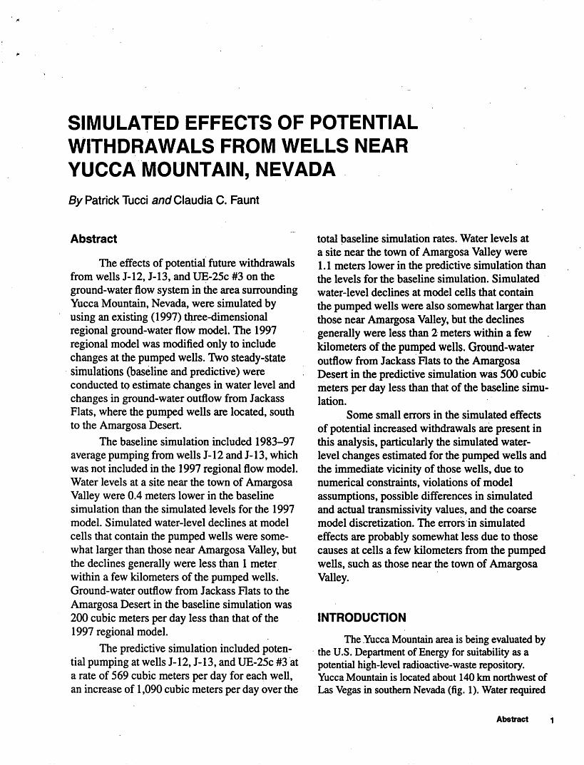
The Yucca Mountain area is being evaluated by the U.S. Department of Energy for suitability as a potential high-level radioactive-waste repository. Yucca Mountain is located about 140 km northwest of Las Vegas in southern Nevada (fig. 1). Water required

Abstract

p*%,

*f.;UmnculTiShKied-ftiicf b«e frm 1:250.000^c»lc Difal Qevttoi Modd; B ilhimii»tiao fron ooftfaeMt n 30 <k|n«« above baciaB

25 0 25

25 25

50 KILOMETERS

SO MILES

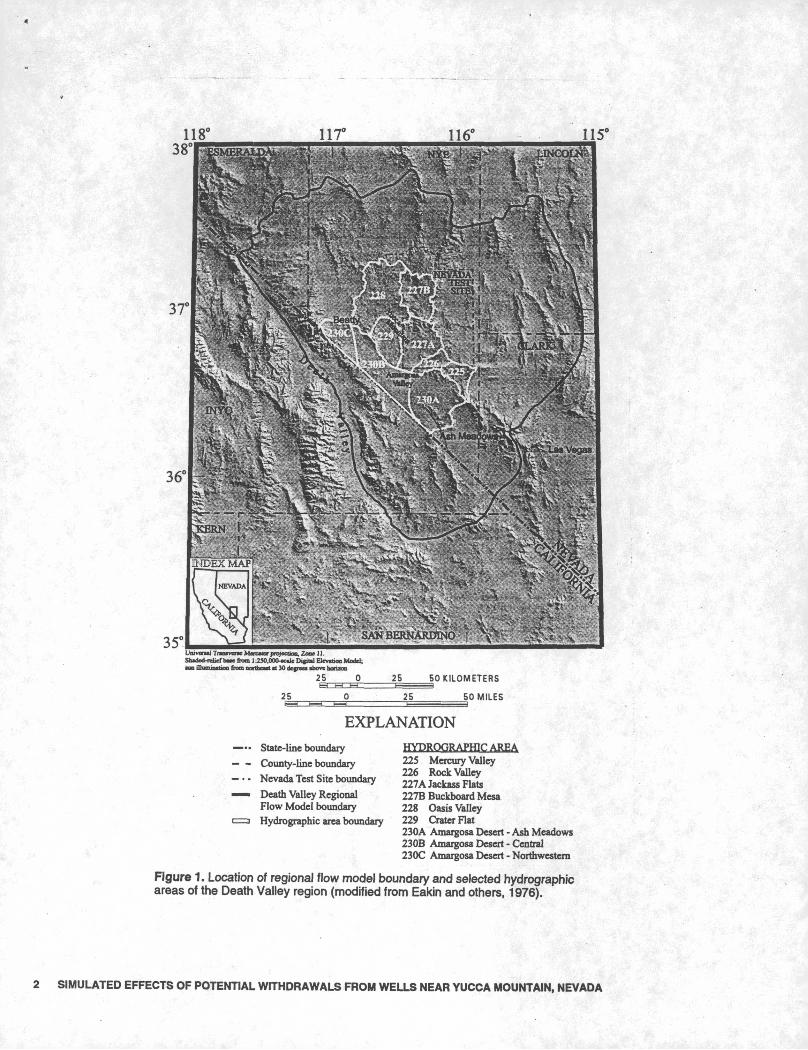
EXPLANATION State-line boundary

- County-line boundary Nevada Test Site boundary Death Valley Regional

Flow Model boundary

HYDROGRAPHIC AREA225 Mercury Valley226 Rock Valley 227A Jackass Flats 227B Buckboard Mesa 228 Oasis Valley

, i i Hydrographic area boundary 229 Crater Flat --." ,. 230A Amargosa Desert - Ash Meadows

230B Amargosa Desert - Central - - ' 230C Amargosa Desert - Northwestern

Figure 1. Location of regional flow model boundary and selected hydrographic areas of the Death Valley region (modified from Eakin and others, 1976).

'*. J..

2 SIMULATED EFFECTS OF POTENTIAL WITHDRAWALS FROM WELLS NEAR YUCCA MOUNTAIN, NEVADA

for the construction and operation of a potential repos itory may be provided by three existing wells J-12, J-13, and UE-25c #3 (fig. 2). The U.S. Department of Energy (DOE) filed applications with the Nevada State Engineer in 1997 to appropriate water to replace existing DOE water-right permits that were issued for site-characterization work. The effects of potential ground-water withdrawals associated with these permits on the ground-water resources of the Amar- gosa Desert south of Yucca Mountain may be of concern to residents of the area and to DOE. The U.S. Geological Survey, in cooperation with DOE under Interagency Agreement DE-AI08-97NV12033, assessed the potential impacts of withdrawals from these wells on the ground-water flow system.

Purpose and Scope

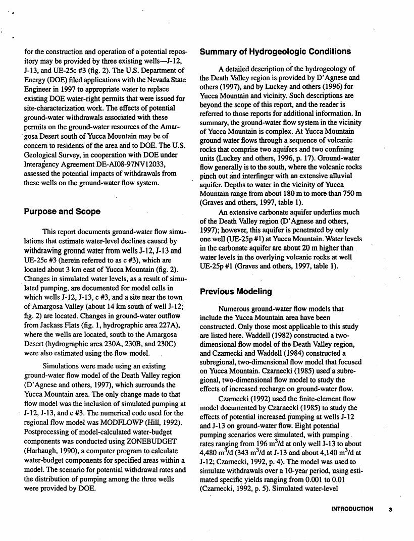
This report documents ground-water flow simu lations that estimate water-level declines caused by withdrawing ground water from wells J-12, J-13 and UE-25c #3 (herein referred to as c #3), which are located about 3 km east of Yucca Mountain (fig. 2). Changes in simulated water levels, as a result of simu lated pumping, are documented for model cells in which wells J-12, J-13, c #3, and a site near the town of Amargosa Valley (about 14 km south of well J-12; fig. 2) are located. Changes in ground-water outflow from Jackass Flats (fig. 1, hydrographic area 227A), where the wells are located, south to the Amargosa Desert (hydrographic area 230A, 230B, and 230C) were also estimated using the flow model.

Simulations were made using an existing ground-water flow model of the Death Valley region (D'Agnese and others, 1997), which surrounds the Yucca Mountain area. The only change made to that flow model was the inclusion of simulated pumping at J-12, J-13, and c #3. The numerical code used for the regional flow model was MODFLOWP (Hill, 1992). Postprocessing of model-calculated water-budget components was conducted using ZONEBUDGET (Harbaugh, 1990), a computer program to calculate water-budget components for specified areas within a model. The scenario for potential withdrawal rates and the distribution of pumping among the three wells were provided by DOE.

Summary of Hydrogeologic Conditions

A detailed description of the hydrogeology of the Death Valley region is provided by D'Agnese and others (1997), and by Luckey and others (1996) for Yucca Mountain and vicinity. Such descriptions are beyond the scope of this report, and the reader is referred to those reports for additional information. In summary, the ground-water flow system in the vicinity of Yucca Mountain is complex. At Yucca Mountain ground water flows through a sequence of volcanic rocks that comprise two aquifers and two confining units (Luckey and others, 1996, p. 17). Ground-water flow generally is to the south, where the volcanic rocks pinch out and interfinger with an extensive alluvial aquifer. Depths to water in the vicinity of Yucca Mountain range from about 180 m to more than 750 m (Graves and others, 1997, table 1).

An extensive carbonate aquifer underlies much of the Death Valley region (D'Agnese and others, 1997); however, this aquifer is penetrated by only one well (UE-25p #1) at Yucca Mountain. Water levels in the carbonate aquifer are about 20 m higher than water levels in the overlying volcanic rocks at well UE-25p #1 (Graves and others, 1997, table 1).

Previous Modeling

Numerous ground-water flow models that include the Yucca Mountain area have been constructed. Only those most applicable to this study are listed here. Waddell (1982) constructed a two- dimensional flow model of the Death Valley region, and Czamecki and Waddell (1984) constructed a subregional, two-dimensional flow model that focused on Yucca Mountain. Czarnecki (1985) used a subre gional, two-dimensional flow model to study the effects of increased recharge on ground-water flow.

Czarnecki (1992) used the finite-element flow model documented by Czarnecki (1985) to study the effects of potential increased pumping at wells J-12 and J-13 on ground-water flow. Eight potential pumping scenarios were simulated, with pumping rates ranging from 196 m3/d at only well J-13 to about 4,480 n//d (343 m3/d at J-13 and about 4,140 m3/d at J-12; Czarnecki, 1992, p. 4). The model was used to simulate withdrawals over a 10-year period, using esti mated specific yields ranging from 0.001 to 0.01 (Czarnecki, 1992, p. 5). Simulated water-level

INTRODUCTION

11T.QJ 3T07'30"

3TOO'

116°45' 116*30' . 116°00'55

60

"'65

.'

115

50 55 60 65 70 75 80 85 90 95ItavaMlTnuMww Mentorpn>fectiai,Zaie 11- . j-isvr TTHOTkT Sb«Joi-rcl.rfb..f from lJJO,000-«»lcDiJit»IEJcv«x» Maid, L-LJL/UIV1INcm ilhnnmaliGB feco Mrthcut at 30 defreei tborc haraaa

0 4 8 12 16 20 KILOMETERS > "" I > H h ' H i i

0 4 8 12 16 20 MILES

.;- ..*^-,;,' %-, , -X '\.-; '-'.' ' . . EXPLANATION :,;. . :- --.,... ' «.. " _( - ".' .. " '

" ! f . --- Nevada Test Site Boundary

"'. - " State-line Boundary c

* ° Observation or pumped well

Figure 2. Location of selected wells and model grid cells near Yucca Mountain.; * :,.* -?: ,

INTRODUCTION

declines after 10 years, using a specific yield of 0.01 and the maximum simulated pumping rates at J-12 and J-13, were 3.5 m at J-13,3.4 m at J-12, and 2.4 m at a site about 2 km northwest of Amargosa Valley.

D'Agnese and others (1997) constructed a three-dimensional ground-water flow model of the Death Valley region, which is used in this study. That model (herein referred to as the 1997 regional flow model) is briefly described in a subsequent section of this report.

Description of Wells J-12, J-13, and UE-25C #3

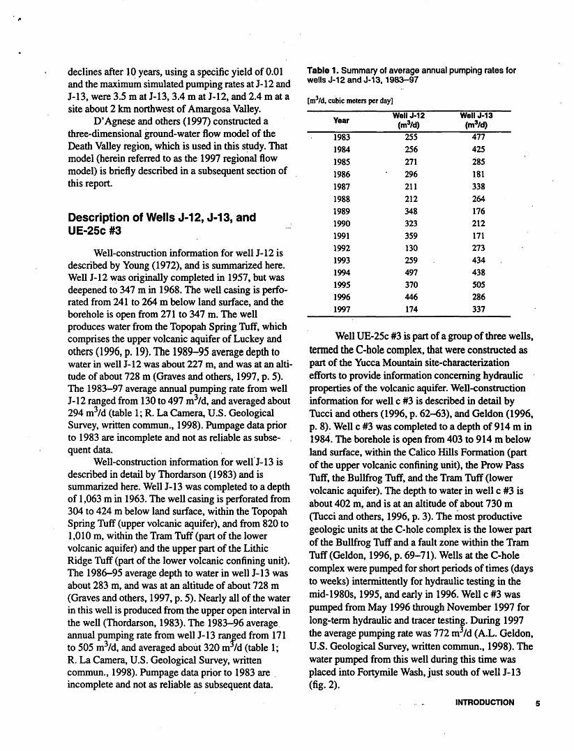
Well-construction information for well J-12 is described by Young (1972), and is summarized here. Well J-12 was originally completed in 1957, but was deepened to 347 m in 1968. The well casing is perfo rated from 241 to 264 m below land surface, and the borehole is open from 271 to 347 m. The well produces water from the Topopah Spring Tliff, which comprises the upper volcanic aquifer of Luckey and others (1996, p. 19). The 1989-95 average depth to water in well J-12 was about 227 m, and was at an alti tude of about 728 m (Graves and others, 1997, p. 5). The 1983-97 average annual pumping rate from well J-12 ranged from 130 to 497 m3/d, and averaged about 294 m3/d (table 1; R. La Camera, U.S. Geological Survey, written commun., 1998). Pumpage data prior to 1983 are incomplete and not as reliable as subse- . quent data.

Well-construction information for weir J-13 is described in detail by Thordarson (1983) and is summarized here. Well J-13 was completed to a depth of 1,063 m in 1963. The well casing is perforated from 304 to 424 m below land surface, within the Topopah Spring Tuff (upper volcanic aquifer), and from 820 to 1,010 m, within the Tram Tuff (part of the lower volcanic aquifer) and the upper part of the Lithic Ridge Tuff (part of the lower volcanic confining unit). The 1986-95 average depth to water in well J-13 was about 283 m, and was at an altitude of about 728 m (Graves and others, 1997, p. 5). Nearly all of the water in this well is produced from the upper open interval in the well (Thordarson, 1983). The 1983-96 average annual pumping rate from well J-13 ranged from 171 to 505 m3/d, and averaged about 320 rn^d (table 1; R. La Camera, U.S. Geological Survey, written commun., 1998). Pumpage data prior to 1983 are incomplete and not as reliable as subsequent data.

Table 1. Summary of average annual pumping rates for wells J-12 and J-13,1983-97

[m3/d, cubic meters per day]

Year

198319841985198619871988198919901991199219931994199519961997

Well J-12 (m3/d)255256271296211212348323359130259497370446174

Well J-13 (m3/d)477425285181338264176212171273434438505286337

Well UE-25c #3 is part of a group of three wells, termed the C-hole complex, that were constructed as part of the Yucca Mountain site-characterization efforts to provide information concerning hydraulic properties of the volcanic aquifer. Well-construction information for well c #3 is described in detail by TAicci and others (1996, p. 62-63), and Geldon (1996, p. 8). Well c #3 was completed to a depth of 914 m in 1984. The borehole is open from 403 to 914 m below land surface, within the Calico Hills Formation (part of the upper volcanic confining unit), the Prow Pass Tuff, the Bullfrog TAiff, and the Tram 1\iff (lower volcanic aquifer). The depth to water in well c #3 is about 402 m, and is at an altitude of about 730 m (Tucci and others, 1996, p. 3). The most productive geologic units at the C-hole complex is the lower part of the Bullfrog 1\iff and a fault zone within the Tram Tuff (Geldon, 1996, p. 69-71). Wells at the C-hole complex were pumped for short periods of times (days to weeks) intermittently for hydraulic testing in the mid-1980s, 1995, and early in 1996. Well c #3 was pumped from May 1996 through November 1997 for long-term hydraulic and tracer testing. During 1997 the average pumping rate was 772 m3/d (A.L. Geldon, U.S. Geological Survey, written commun., 1998). The water pumped from this well during this time was placed into Fortymile Wash, just south of well J-13 (fig. 2).

INTRODUCTION

SIMULATED EFFECTS OF POTENTIAL WITHDRAWALS

The effects of potential withdrawals on the ground-water flow system in the vicinity of Yucca Mountain were simulated using the 1997 regional flow model, described in detail by D'Agnese and others (1997). The simulation strategy was to update that model by inclusion of long-term (1983-97), average pumping at wells J-12 and J-13 and to use that modi- fled model as a baseline to estimate the effects of potential changes in withdrawals at Yucca Mountain. The following sections provide a summary description of the 1997 regional model, describe modifications made to that model for this study, and describe the results of two simulations.

Description of the 1997 Regional Flow Model

The 1997 Death Valley regional ground-water flow model was constructed to provide a better under standing of the regional flow system and to provide boundary information for a smaller, site-scale flow model. A detailed description of the regional flow model is provided by D'Agnese and others (1997), and a summary of model geometry, boundary conditions, and model calibration is presented in the following paragraphs.

The numerical code used for the 1997 regional flow model was MODFLOWP (Hill, 1992). MODFLOWP is an adaptation of the U.S. Geological Survey finite-difference, modular ground-water flow model, MODFLOW (McDonald and Harbaugh, 1988) in which nonlinear regression is used to estimate flow- model parameters that result in the best fit to measured hydraulic heads and flows (Hill, 1992). MODFLOWP is a block-centered finite-difference code that views a three-dimensional flow system as a sequence of porous-material layers.

The 1997 regional model consists of a finite- difference grid of 163 rows, 153 columns, and 3 layers. The grid is oriented north-south and the cells are of uniform size in both N-S and E-W directions, with dimensions of 1,500 m. The layers represent conditions at 0-500 m (upper layer), 500-1,250 m (middle layer), and 1,250-2,750. m (lower layer) below the estimated regional potentiometric surface. The upper and middle layers simulate local and subregional ground-water flow within valley-fill alluvium,

volcanic rocks, and shallow carbonate rocks. The lower layer simulates deep, regional ground-water flow in volcanic, carbonate, and clastic rocks.

All lateral boundaries in the upper layer were designated as no-flow, except along the western side of the model in Death Valley where constant-head values were designated. No ground water is believed to enter or exit the Death Valley regional flow system at inter mediate depths, so that all lateral boundaries in the middle layer were set to no-flow. In the lower layer, the lateral boundaries were designated as no-flow except at four locations along the northern and eastern limits of the model, where they were designated as constant-head boundaries because the conceptual model suggests interconnections with adjacent systems along buried zones of higher permeability. The upper boundary of the flow model is the estimated regional potentiometric surface. The lower boundary is set at a depth of 2,750 m below the estimated regional potentiometric surface and is designated as no-flow because few fractures are believed to be open to allow significant amounts of ground-water flow. Internal boundary conditions include areally distrib uted recharge from precipitation, evapotranspiration, spring flow, and pumping from wells. Pumping from wells J-12, J-13, and c #3, however, was not included in the 1997 flow model, because reliable pumpage data were not available for those wells at the time model construction began (F.A. D'Agnese, U.S. Geological Survey, oral commun., 1998).

Two important assumptions are incorporated in the model: (1) Flow through the mostly fractured-rock aquifers can be adequately simulated as a porous- medium equivalent, and (2) the long-term average hydrologic conditions can be simulated as steady-state conditions. D'Agnese and others (1997, p. 72) discuss these assumptions in detail.

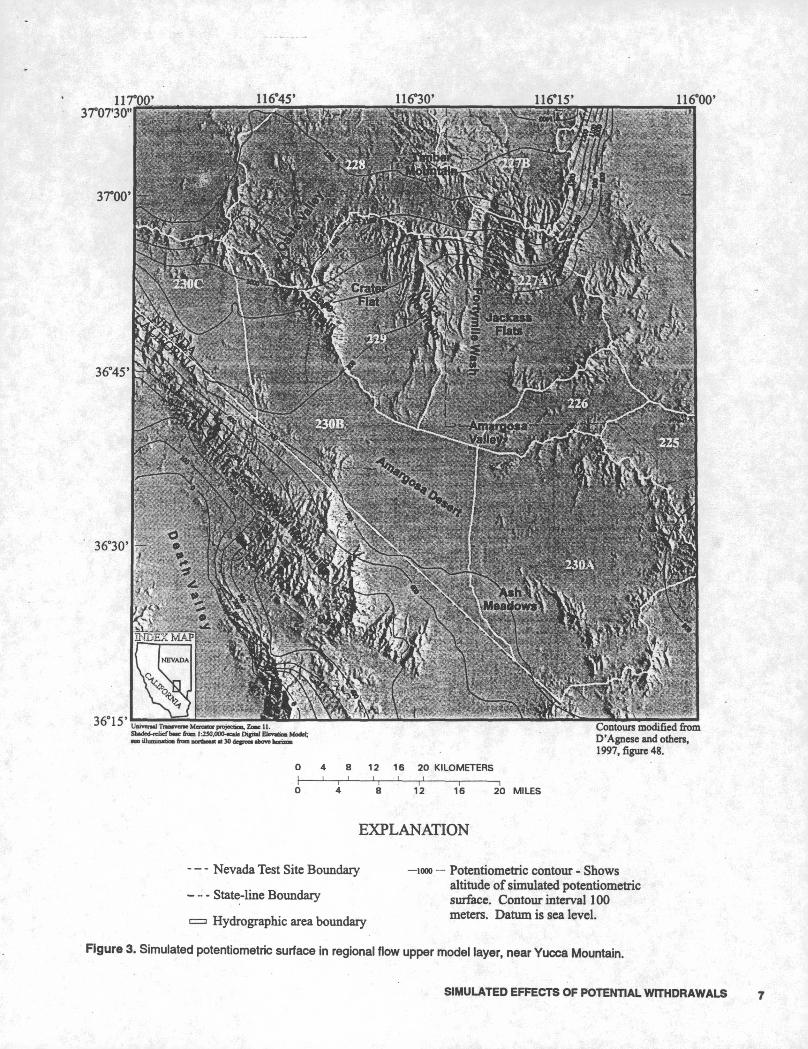
The model was calibrated to observed water levels at 500 wells and to measured or estimated flow at 63 springs. The calibrated model depicts major features of the observed or estimated head distribution, such as areas of large and small hydraulic gradients, reasonably well (fig. 3). Residuals between observed and simulated water levels were smallest in areas of small hydraulic gradients. Residuals at wells J-12 and J-13 were -18.2 m and -18.8 m, respectively. Resid uals in other parts of Jackass Rats and in the northern part of the Amargosa Desert generally ranged from about -4 to -30 m. These negative residuals indicate that simulated water levels are higher than observed levels.


11 TOO 3T07'30"116°45' 116°30' He'15' new

3TOO

Univvml Tnwcne Manor projection. Zooe 11. Sk^fe)-rebrfb«tfrooi I^SO.OOO-KakDlfinlEJcyMiaiM mo iUumuulxai froa ncflfaaut tt 30 degreei *bow horizon

Contours modified from D'Agnese and others, 1997, figure 48.

0 4 8 12 16 20 KILOMETERS

8 12 16 20 MILES

EXPLANATION

---Nevada Test Site Boundary

k _... State-line Boundary

a Hydrographic area boundary

Figure 3. Simulated potentiometric surface in regional flow upper model layer, near Yucca Mountain.

looo Potentiometric contour - Showsaltitude of simulated potentiometric surface. Contour interval 100 meters. Datum is sea level. ,»,,.,


The simulated rate of ground-water outflow through all model layers from Jackass Flats to the Amargosa Desert in the 1997 model was about 18,300 m3/d. Of this total, outflow through the upper model layer was 223 m3/d> outflow from the middle layer was 1,400 m3/d, and outflow from the lower layer was about 16,700 m3/d.

Modification to the 1997 Regional Flow Model

The only change made to the 1997 regional model for this study was the addition of simulated pumping from model cells that contain wells J-12, J-13, and c #3. Simulated pumping was assigned to the upper model layer for each of the wells, at the rate appropriate for the simulation (table 2). Although well J-13 is completed to a depth corresponding to layer 2 of the regional model, no pumping was simulated from that layer because nearly all of the production from the well is from the upper open interval (Thordarson, 1983). No additional calibration of the 1997 regional model was attempted with the addition of the pumped wells.

Baseline Simulation

The first (baseline) simulation included 1983- 97 average pumping at wells J-12 and J-13, which was not included in the 1997 regional flow model. Pumping from well c #3 was not included in this simu lation because of the intermittent nature and relatively small volume of water pumped in relation to long-term pumping at wells J-12 and J-13. Simulated pumping rates were 294 m3/d for well J-12 and 320 m3/d for well J-13 (table 2). Because inclusion of the long-term average pumping at wells J-12 and J-13 in the baseline simulation is probably more representative of existing ground-water conditions than those in the 1997 regional flow model, output from the baseline simula tion (water levels and water-budget components) was used as a starting point for the subsequent predictive simulation.

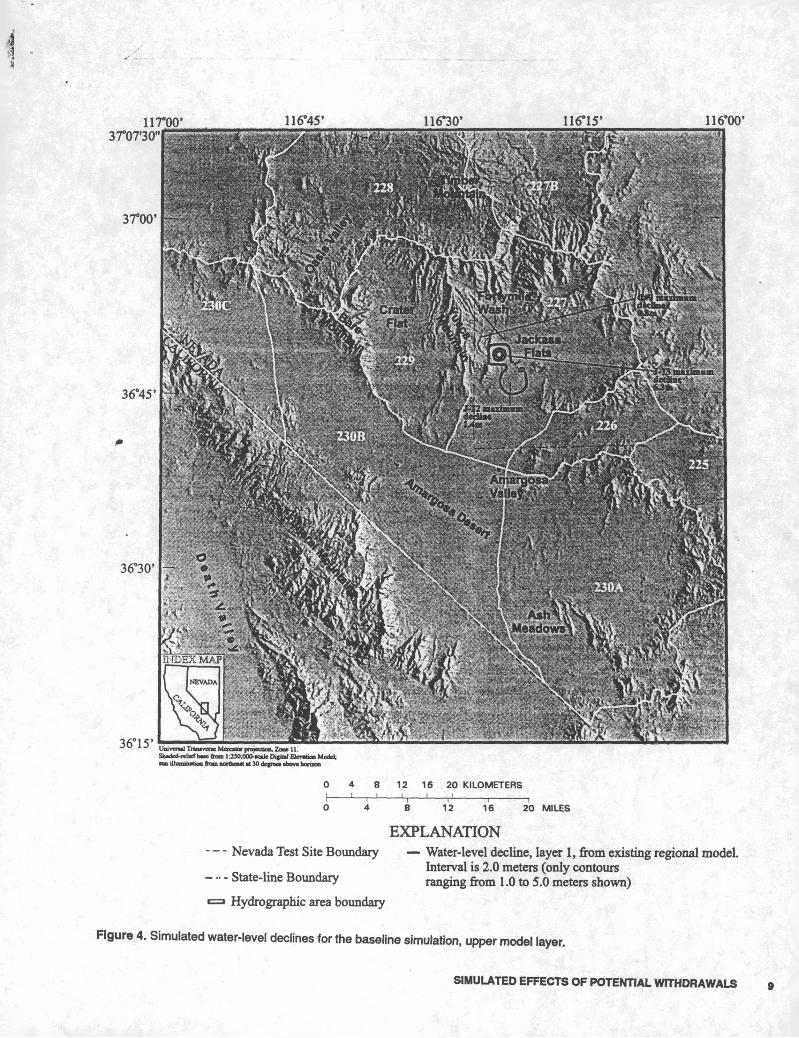
Differences in simulated water-levels from those of the 1997 regional model were largest in the vicinity of wells J-12 and J-13, and were generally less than 1 m within a few kilometers of the simulated wells (fig. 4). Simulated water-level differences at a model cell (row 90, column 76; fig. 2) near the town of Amar gosa Valley was -0.4 m in each of the model layers (table 2). Simulated water-level differences from the 1997 regional flow model were greater in the cells

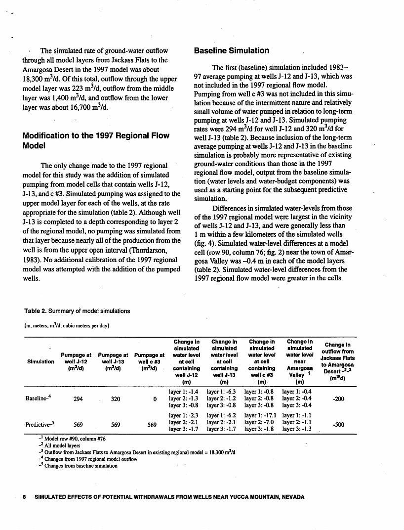
Table 2. Summary of model simulations

[m, meters; m3/d, cubic meters per day]

Simulation

Baseline-4

Predictive-5

Pumpage at wellJ-12

(m3/d)

294

569

Pumpage at well J-13

(m3/d)

320

569

Pumpage at well c #3

(m3/d)

0

569

Change in simulated

water level at cell

containing well J-12

(m)

layer 1:-1.4 layer 2: -1.3 layer 3: -0.8

layer 1: -2.3 layer 2: -2.1 layer 3: -1.7

Change In simulated

water level at cell

containing well J-13

(m)



Change In simulated

water level at cell

containing well c #3

(m)



Change In simulated

water level near

Amargosa Valley-1

(m)



Change In outflow from Jackass Flats to Amargosa Desert-2-3

(m^d)

-200

-500

-1 Model row #90, column #76-2 All model layers-3 Outflow from Jackass Flats to Amargosa Desert in existing regional model = 18,300 m3/d-4 Changes from 1997 regional model outflow-5 Changes from baseline simulation


iiroo*3TOT30"

116°45' 116*30' lie-is- 116°00'

3TOO'

36°15 Untvml TMmne Kbnttoc prejocooo, Zmc 11. Sludal-relitf b«e from 1:250.00fr«cik DiJittI EtoM» Mold; »ilhnmoMia ten Donhaut u 30 derm ibovi korani

0 4 B 12 16 20 KILOMETERS

8 12 16 20 MILES

;';. ; ' EXPLANATION *'-: -m^ & . *--- Nevada Test Site Boundary Water-level decline, layer 1, from existing regional model.

Interval is 2.0 meters (only contours- -State-line Boundary ranging from 1 .0 to 5.0 meters shown) -^

.: "" ' ' .- _. "-^ -,_,/,-.'; -*$. . ^ ' .

J f,-- «=» Hydrographic area boundary ,^ t^ ^ ?"'*-*- ''"*' > . ,.>^ -r* ,, ; ,':f ̂ '; fE:A fe:;'Figure 4. Simulated water-level declines for the baseline simulation, upper model layer. "* ' *! ^^ ?

' '.' ' . '-'I' '">-.!" ": 5 . ..'.-: 'i? '- .'**


containing the pumped wells (-6.3 m for J-13 and -1.4 m for J-12, in the upper layer; table 2); however, the differences for the pumped-well cells are probably underestimated by the model, as discussed in more detail in the Model Limitations and Discussion section.

Simulated ground-water outflow from Jackass Flats to the Amargosa Desert was 18,100 m3/d, a reduction of 200 m3/d from the simulated outflow in the 1997 model (table 2). Most of this reduction occurred in the lower model layer.

Inclusion of the long-term average pumping at these wells in the baseline simulation resulted in a slight improvement in the regional model, in that residuals between simulated and measured water levels were reduced. In the 1997 regional model resid uals at J-12 and J-13 were -18.2 m and -18.8 m, respectively; however, residuals for the baseline simu lation were -16.8 m at J-12 and -15.1 m at J-13.

Simulation of Increased Withdrawals

The second simulation (herein termed the predictive simulation) increased the pumping rate at wells J-12, J-13, and c #3 to 569 m3/d from each well. The total pumping rate from these wells for this simu lation is, therefore, about 1,710 m /d. This amount represents the change in pumping rates requested by DOE for water appropriation (1,450 m3/d) plus an amount (255 m3/d) assumed by DOE to represent ground-water withdrawals not under existing permits for the Nevada Test Site. This total amount of pumping is about 1,090 m3/d greater than the total 1983-97 average pumping rate at wells J-12 and J-13. Water levels and flow components from the predictive simulation were compared to those of the baseline simulation, which is considered to be representative of existing hydrologic conditions.

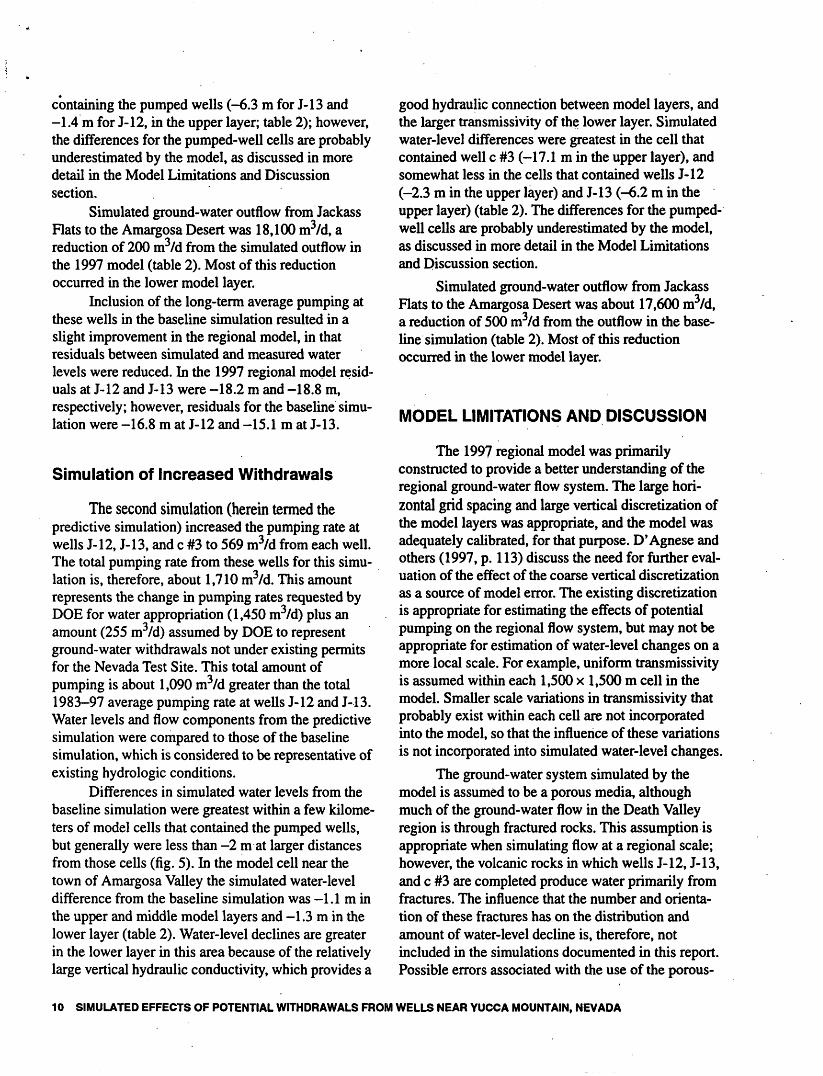
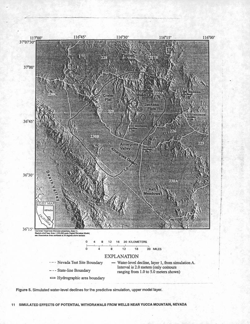
Differences in simulated water levels from the baseline simulation were greatest within a few kilome ters of model cells that contained the pumped wells, but generally were less than -2 m at larger distances from those cells (fig. 5). In the model cell near the town of Amargosa Valley the simulated water-level difference from the baseline simulation was -1.1 m in the upper and middle model layers and -1.3 m in the lower layer (table 2). Water-level declines are greater in the lower layer in this area because of the relatively large vertical hydraulic conductivity, which provides a

good hydraulic connection between model layers, and the larger transmissivity of the lower layer. Simulated water-level differences were greatest in the cell that contained well c #3 (-17.1 m in the upper layer), and somewhat less in the cells that contained wells J-12 (-2.3 m in the upper layer) and J-13 (-6.2 m in the upper layer) (table 2). The differences for the pumped- well cells are probably underestimated by the model, as discussed in more detail in the Model Limitations and Discussion section.

Simulated ground-water outflow from Jackass Flats to the Amargosa Desert was about 17,600 m3/d, a reduction of 500 m3/d from the outflow in the base line simulation (table 2). Most of this reduction occurred in the lower model layer.

MODEL LIMITATIONS AND DISCUSSION

The 1997 regional model was primarily constructed to provide a better understanding of the regional ground-water flow system. The large hori zontal grid spacing and large vertical discretization of the model layers was appropriate, and the model was adequately calibrated, for that purpose. D'Agnese and others (1997, p. 113) discuss the need for further eval uation of the effect of the coarse vertical discretization as a source of model error. The existing discretization is appropriate for estimating the effects of potential pumping on the regional flow system, but may not be appropriate for estimation of water-level changes on a more local scale. For example, uniform transmissivity is assumed within each 1,500 x 1,500 m cell in the model. Smaller scale variations in transmissivity that probably exist within each cell are not incorporated into the model, so that the influence of these variations is not incorporated into simulated water-level changes.

The ground-water system simulated by the model is assumed to be a porous media, although much of the ground-water flow in the Death Valley region is through fractured rocks. This assumption is appropriate when simulating flow at a regional scale; however, the volcanic rocks in which wells J-12, J-13, and c #3 are completed produce water primarily from fractures. The influence that the number and orienta tion of these fractures has on the distribution and amount of water-level decline is, therefore, not included in the simulations documented in this report. Possible errors associated with the use of the porous-


11 TOO' STOT'SO"

116*45' 116*30' 116*15' 116*00'

sroo1

36°45'

36°30'

36"15'UmverwU Traotvcnc Mercaior pnjjocaon. Loot 11. Sbadod-rebef bne frwn 1.250,000-KaJe Dtfitxl Elcvvbon Model,

t 30 <te|na *bovc harnoa

»^ 0 4 8 12 16 20 KILOMETERS

: "' ' "" I > H h ' H i ,0 4 8 12 16 20 MILES

* '* ' EXPLANATION r *

Nevada Test Site Boundary Water-level decline, layer 1, from simulation A.

State-line Boundary

Hydrographic area boundary

Interval is 2.0 meters (only contoursranging from 1.0 to 5.0 meters shown) , ;

Figure 5. Simulated water-level declines for the predictive simulation, upper model layer.

11 SIMULATED EFFECTS OF POTENTIAL WrTHDRAWALS FROM WELLS NEAR YUCCA MOUNTAIN, NEVADA

''4-

media assumption are probably greatest within a few kilometers of the simulated pumped wells.

The steady-state assumption used in the model may be another source of error. D'Agnese and others (1997, p. 72) discuss four possible conditions that may violate this assumption; however, for the purpose of the 1997 regional model, errors associated with these conditions are believed to be acceptable. Steady-state conditions were also simulated in this study, so that the effects of aquifer storage and time-variant hydrologic conditions (such as climate variations or changes in regional pumping) are not included in the water- level change estimated by the model.

In the baseline simulation, the 1983-97 average pumping rates for wells J-12 and J-13 are assumed to be representative of steady-state conditions. If this assumption is not valid, then the difference in water- levels between the 1997 model and the baseline simu lation could be overestimated. Likewise, if the poten tial increased pumping represented in the predictive simulation would be terminated before steady-state conditions were reached, then the differences in water levels between that simulation and the baseline simu lation will also be overestimated. Use of the steady- state assumption will, therefore, tend to provide conservative estimates of water-level declines due to potential pumping-rate increases. The steady-state assumption is considered to be appropriate for this study because the requested water appropriation by DOE is for a long-term water right.

Transmissivity values used in the 1997 regional flow model were not changed for this study. Transmis sivity values in the upper layer of the model are about 3 m2/d in the vicinity of J-12, J-13, and c #3. Hydraulic tests conducted during 1996-97 at the C-hole complex, however, indicate transmissivity values ranging from 2,140 to 2,600 m2/d for the sequence of volcanic rocks present in that area (A.L. Geldon, U.S. Geological Survey, written commun., 1997). Thordarson (1983) estimated the transmissivity of the rocks corresponding to the upper model layer at well J-13 to be about 120 m2/d. Hydraulic tests conducted at well JF-3, which is about 1,200 m south of J-12 (fig. 2), resulted in transmissivity estimates for the volcanic rocks at that site that range from about 13,000 to 14,900 m2/d (Plume and La Camera, 1996, p. 17). Because the transmissivity values used in the model are much smaller than other estimates of trans missivity for this area, simulated steady-state water- level declines due to potential pumping probably are

overestimated, particularly near the pumped wells. Drawdowns measured during hydraulic tests conducted at the C-well complex in 1996-97 may support this conclusion. Drawdown at the pumped well (c #3) after 18 months of pumping at an average rate of 772 m3/d was about 6 m and was less than 1 m within a kilometer of the pumped well (A.L. Geldon, U.S. Geological Survey, written commun., 1997). Simulated steady-state drawdowns for the predictive simulation, in which well c #3 was pumped at a lower rate (569 m3/d) were much greater (-17.1 m) than those observed during the 18-month hydraulic tests.

Uniform transmissivity values within a cell are assumed in the model code. Features that are smaller scale than the model grid cell cannot accurately be represented by the model. For example, a large percentage of the water pumped from well c #3 is produced from a fault zone in the Tram Tuff near the bottom of the well (Geldon, 1996). This highly transmissive feature is not represented in the model; however, applying the large transmissivity associated with this small-scale feature over the entire 1.13 x 109 m3 grid cell would also not be appropriate. The actual transmissivity of the aquifer, represented by this model cell, is probably less than the values obtained from the aquifer tests.

In MODFLOWP, a pumped well is assumed to fully penetrate the aquifer and to be open to the aquifer throughout the entire saturated interval; however, such conditions do not exist at wells J-12, J-13, and c #3. Because these wells may not access all of the water- producing zones within the volcanic rock aquifer, actual water-level declines at and in the immediate vicinity of the pumped well will be greater than simu lated declines.

Additionally, the finite-difference method used in the model does not accurately calculate water- level declines at the pumped wells, because the grid dimensions are much larger than the well diameter (Anderson and Woessner, 1992, p. 147; Planert, 1997, p. 2). This inaccuracy is because the finite-difference approximation applies the pumping to the entire grid cell, rather than to a well at the center of the cell. Simulated water-level gradients within the cell are much smaller than the actual gradients, which can be quite large close to the pumped well. The model also does not take into account well-bore losses, which can increase the drawdown within a pumped well. In summary, the simulated water-level declines in the cells containing the pumped wells will be underesti-


mated due to numerical constraints in the model code, however, water-levels at grid cells at some distance from the pumped wells will be simulated more accu rately (Anderson and Woessner, 1992, p. 147).

Another source of error in the simulated water- level changes is the location of the pumped well within a model grid cell. The well is assumed to be at the center of the cell; however, the actual location of wells J-12, J-13, and c #3 are not at the centers of the cells in which they are simulated. The positions of contours of simulated water-level change, shown in figures 4 and 5, could be as much as 750 m (half the grid-cell dimension) in error due to this difference in pumped well location.

Direct comparison of water-level changes simu lated by Czarnecki (1992) to those of this study is not appropriate. Water-level declines estimated by Czar necki (1992, p. 19) were for a 10-year simulation period, rather than for steady-state conditions. Pumping rates simulated by Czarnecki (1992, p. 4) also were different from those used in this study, and no pumping was simulated from c #3 in his analysis.

In summary, some small errors in the simulated effects of potential increased withdrawals are present in this analysis, particularly the simulated water-level changes estimated for the pumped wells and in the immediate vicinity of those wells, due to numerical constraints, violations of model assumptions, possible differences in simulated and actual transmissivity values, and the coarse model discretization. The errors in simulated effects are probably somewhat less due to those causes at cells a few kilometers from the pumped wells, such as those near the town of Amar- gosa Valley. Within the limitations discussed in this section, the modified regional flow model probably provides a reasonable estimate of the effects of poten tial increased ground-water withdrawals at Yucca Mountain, particularly at large distances from the pumped wells in the Amargosa Desert.

SUMMARY

The U.S. Department of Energy filed an applica tion with the State of Nevada in 1997 to appropriate water by pumping three existing wells in the vicinity of Yucca Mountain, Nevada. The effects of potential withdrawals from wells J-12, J-13, and UE-25c #3 on the ground-water flow system in the area surrounding and south of Yucca Mountain were simulated by using

an existing (1997) three-dimensional regional flow model.

The 1997 model was originally constructed to provide a better understanding of the Death Valley regional ground-water flow system and to provide boundary information for a smaller, site-scale flow model. The model is made up of grid cells that are 1,500 m on a side, and three layers that represent ground-water conditions at 0-500 m, 500-1,250 m, and 1,250-2,750 m below the estimated regional potentiometric surface. Steady-state ground-water conditions are assumed in the 1997 model, and the model was calibrated to observed water levels at 500 wells and to measured or estimated flow at 63 springs in the region.

The only change made to the 1997 flow model for this study was the addition of wells, not included in the 1997 model, to simulate pumping from wells J-12, J-13, and c #3. Changes in simulated water level were evaluated at the pumped wells and at a site about 14 km south of wells J-12, near the town of Amargosa Valley. Changes in simulated water levels and ground- water outflow from Jackass Flats to the Amargosa Desert were evaluated in two (baseline and predictive) model simulations.

The baseline simulation included long-term average pumping from wells J-12 and J-13, which was believed to better represent existing hydrogeologic conditions than the 1997 regional model. Water levels at a site near the town of Amargosa Valley were 0.4 m lower in the baseline simulation than the simulated levels for the 1997 model as a result of the addition of pumping at J-12 and J-13. Simulated water-level declines at model cells that contain the pumped wells were somewhat larger than those near Amargosa Valley, but the declines generally were less than 1 m within a few kilometers of the pumped wells. Simu lated declines generally were greater in the upper model layer than in the middle and lower model layers. Ground-water outflow from Jackass Flats to the Amargosa Desert in the baseline simulation was 200 m3/d less than that of the 1997 regional model.

The predictive simulation included potential pumping at wells J-12, J-13, and UE-25c #3 at a rate of 569 m3/d for each well, an increase of 1,090 m3/d over the total baseline simulation rates. Water levels at a site near the town of Amargosa Valley were l.lm lower in the predictive simulation than the levels for the baseline simulation as a result of the increased pumping rate at J-12, J-13, and c #3. Simulated water-

SUMMARY 13

level declines at model cells that contain the pumped wells were also larger than those near Amargosa Valley, but the declines generally were less than 2 m within a few kilometers of the pumped wells. Simu lated declines generally were greater in the upper model layer than in the middle and lower model layers. Ground-water outflow from Jackass Flats to the Amargosa Desert in the predictive simulation was 500 m3/d less than that of the baseline simulation.

Some small errors in the simulated effects of potential increased withdrawals are present in this analysis, particularly the simulated water-level changes estimated for the pumped wells and in the immediate vicinity of those wells, due to numerical constraints, violations of model assumptions, possible differences in simulated and actual transmissivity values, and the coarse model discretization. The errors in simulated effects are probably somewhat less due to those causes at cells a few kilometers from the pumped wells, such as those near the town of Amar gosa Valley. Within the limitations discussed in the report, the modified regional flow model probably provides a reasonable estimate of the effects of poten tial increased ground-water withdrawals at Yucca Mountain, particularly at large distances from the pumped wells in the Amargosa Desert.

REFERENCES CITED

Anderson, M.R, and Woessner, W.W., 1992, Applied . groundwater modeling, simulation of flow and advec-

tive transport: Academic Press, San Diego, California, 381 p.

Czarnecki, J.B., 1985, Simulated effects of increased recharge on the ground-water flow system of Yucca Mountain and vicinity, Nevada-California: U.S. Geological Survey Water-Resources Investigations Report 84-4344, 33 p.

Czarnecki, J.B., 1992, Simulated water-level declines caused by withdrawals from wells J-13 and J-12 near Yucca Mountain, Nevada: U.S. Geological Survey Open-File Report 91-478,20 p.

Czarnecki, J.B., and Waddell, R.K., 1984, Finite-element simulation of ground-water flow in the vicinity of Yucca Mountain, Nevada-California: U.S. Geolog ical Survey Water-Resources Investigations Report 84-^349, 38 p.

D'Agnese, F.A., Faunt, C.C., Turner, A.K., and Hill, M.C., 1997, Hydrogeologic evaluation and numerical simula tion of the Death Valley regional ground-water flow system, Nevada and California: U.S. Geological Survey Water-Resources Investigations Report 96-^300,124 p.

Eakin, T.E., Price, Don, and Harrill, J.R., 1976, Summary appraisals of the Nation's ground-water resources Great Basin region: U.S. Geological Survey Profes sional Paper 813-Gj, 37 p.

Geldon, A.L., 1996, Results and interpretation of prelimi nary aquifer tests in boreholes UE-25c #1, UE-25c #2, and UE-25c #3, Yucca Mountain, Nye County, Nevada: U.S. Geological Survey Water-Resources Investigations Report 94-4177,119 p.

Graves, R.P., Tucci, Patrick, and O'Brien, G.M., 1997, Analysis of water-level data in the Yucca Mountain area, Nevada, 1985-95: U.S. Geological Survey Water-Resources Investigations Report 96-4256, 140 p.

Harbaugh, A.W., 1990, A computer program for calculating subregional water budgets using the U.S. Geological Survey modular three-dimensional finite-difference ground-water flow model: U.S. Geological Survey Open-File Report 90-392,46 p.

Hill, M.C., 1992, A computer program (MQDFLOWP) for estimating parameters of a transient, three-dimen sional, ground-water flow model using nonlinear regression: U.S. Geological Survey Open-File Report 91-484, 358 p.

Luckey, R.R., Tucci, Patrick, Faunt, C.C., Ervin, E.M., Steinkampf, W.C., D'Agnese, F.A., and Patterson, G.L., 1996, Status of understanding of the saturated- zone ground-water flow system at Yucca Mountain, Nevada, as of 1995: U.S. Geological Survey Water- Resources Investigations Report 96-4077, 71 p.

McDonald, M.G., and Harbaugh, A.W., 1988, A modular three-dimensional finite-difference ground-water flow model: U.S. Geological Survey Techniques of Water- Resources Investigations, Book 6, Chap. Al, 576 p.

Planert, Michael, 1997, Documentation of a computer program to estimate the head in a well of finite radius using the U.S. Geological Survey modular finite differ ence ground-water flow model: U.S. Geological Survey Open-File Report 96-651 A, lip.

Plume, R.W., and La Camera, R.J., 1996, Hydrogeology of rocks penetrated by test well JF-3, Jackass Flats, Nye County, Nevada: U.S. Geological Survey Water- Resources Investigations Report 95-4245,21 p.


Thordarson, William, 1983, Geohydrologic data and test results from well J-13, Nevada Test Site, Nye county, Nevada: U.S. Geological Survey Water-Resources Investigations Report 83-4171,57 p.

1\icci, Patrick, O'Brien, G.M., and Burkhardt, D.J., 1996, Water levels in the Yucca Mountain area, 1990-91: U.S. Geological Survey Open-File Report 94-111, 107 p.

Waddell, R.K., 1982, Two-dimensional, steady-state model of ground-water flow, Nevada Test Site and vicinity, Nevada-California: U.S. Geological Survey Water- Resources Investigations Report 82 4085,72 p.

Young, R.A., 1972, Water supply for the nuclear rocket development station at the U.S. Atomic Energy Commission's Nevada Test Site: U.S. Geological Survey Water-Supply Paper 1938,19 p.

REFERENCES CITED 15

usgs · pdf fileshkied-ftiicf b«e frm 1:250.000^c»lc difal qevttoi modd; b...

Documents