USING A LOGISTIC PHENOLOGY MODEL WITH IMPROVED DEGREE-DAYACCUMULATORS TO FORECAST EMERGENCE OF PEST GRASSHOPPERS

PAUL MICHAEL IRVINEB. Sc. Mathematics, University of Lethbridge, 2003

A ThesisSubmitted to the School of Graduate Studies

of the University of Lethbridgein Partial Fulfillment of the

Requirements for the Degree

MASTER OF SCIENCE

Department of Mathematics and Computer ScienceUniversity of Lethbridge

LETHBRIDGE, ALBERTA, CANADA

c© Paul Irvine, 2011

Dedication

This thesis is dedicated first and foremost to my twin nephews, Benny and Alex, whom I

love very much and who inspire me to be a better person and help make the world a better

place for them to live in. Irvine family motto: Sub Sole Sub Umbra Virens

This thesis is also dedicated to my family, my friends, my love, and all people who have

disabilities (mental and physical) that challenge them on a daily basis. This is dedicated

also to people who rise up in the face of adversity, and thrive anyways.

This thesis is also dedicated to the memory of Patrick Chan, with whom I worked

closely and whom I have many fond memories of. Also this thesis is dedicated to Dr. Jim

(Jiping) Liu, who was an excellent mentor, professor, and friend.

iii

Abstract

Many organisms, especially animals like insects, which depend on the environment for

body heat, have growth stages and life cycles that are highly dependent on temperature.

To better understand and model how insect life history events progress, for example in the

emergence and initial growth of the biogeographical research subjects, we must first under-

stand the relationship between temperature, heat accumulation, and subsequent develop-

ment. The measure of the integration of heat over time, usually referred to as degree-days,

is a widely used science-based method of forecasting, that quantifies heat accumulation

based on measured ambient temperature. Some popular methods for calculation of degree-

days are the traditional sinusoidal method and the average method. The average method

uses only the average of the daily maximum and minimum temperature, and has the ad-

vantage that it is very easy to use. However, this simplest method can underestimate the

amount of degree-day accumulation that is occurring in the environment of interest, and

thus has a greater potential to reduce the accuracy of forecasting insect pest emergence.

The sinusoidal method was popularized by Allen (1976, [1]), and gives a better approxi-

mation to the actual accumulation of degree-days. Both of these degree-day accumulators

are independent of typical heating and cooling patterns during a typical day cycle. To

address possible non-symmetrical effect, it was deemed prudent to construct degree-day

accumulators to take into account phenomena like sunrise, sunset, and solar noon. Con-

sideration of these temporal factors eliminated the assumption that heating and cooling in

a typical day during the growth season is symmetric. In some tested cases, these newer

degree-day integrators are more accurate than the traditional sinusoidal method, and in all

tested cases, these integrators are more accurate than the average method. After developing

the newer degree-day accumulators, we chose to investigate use of a logistic phenology

model similar to one used by Onsager and Kemp (1986, [54]) when studying grasshopper

iv

development. One reason for studying this model is that it has parameters that are important

when considering pest management tactics, such as the required degree-day accumulations

needed for insects in immature stages (instars) to be completed, as well as a parameter re-

lated to the variability of the grasshopper population. Onsager and Kemp used a nonlinear

regression algorithm to find parameters for the model. I constructed a simplex algorithm

and studied the effectiveness when searching for parameters for a multi-stage insect popu-

lation model. While investigating the simplex algorithm, it was found that initial values of

parameters for constructing the simplex played a crucial role in obtaining realistic and bio-

logically meaningful parameters from the nonlinear regression. Also, while analyzing this

downhill simplex method for finding parameters, it was found there is the potential for the

simplex to get trapped in many local minima, and thus produce extraneous or incorrectly

fitted parameter estimates, although Onsager and Kemp did not mention this problem.

In tests of my methods of fitting, I used an example of daily weather data from Onefour,

AB, with a development threshold of 12 ◦C and a biofix day of April 1st, as an example.

The method could be applied to larger, more extensive datasets that include grasshopper

population data on numbers per stage, by date, linked to degree accumulations based on

the non-symmetrical method, to determine whether it would offer significant improvement

in forecasting accuracy of spring insect pest events, over the long term.

v

Acknowledgments

I would like to thank my supervisors Dan Johnson and David Kaminski for taking me on

as a graduate student. Thank you both for believing in me, even when I had my moments

of self doubt. I will be forever grateful for your constant encouragement, patience and

optimism. Also I would like to thank you both for taking time to help me put together this

thesis by reviewing the many drafts it went through and consistently giving me great advice

on matters regarding my research and thesis work.

I would also like to thank the following people:

Dr. John Sheriff- for being a member of my supervisory committee, editing my thesis,

and helping me get through my first T.A. position for his statistics course.

Dr. Danny Le Roy- for also being a member of my supervisory committee and his

helpful comments regarding the structuring of my thesis, as well as giving me the advice to

start my thesis work early.

Dr. Brad Hagen and Bill Peifer- for giving me great advice about life and how to

approach various circumstances. Also for helping me to maintain a healthy balance of

work and play in my life.

Dr. Scott Irvine and Dr. Angela Irvine- for listening to my complaints about being a

graduate student and giving me advice for surviving academia and the challenges brought

forth by a graduate degree. Also for giving me two amazing nephews for whom this thesis

is dedicated.

The late Patrick Chan- for making my days in the office happy ones and for his constant

positive attitude.

Dana Andrei- for helping with printing out stuff when I needed it, and for having some-

one to chat with in the water sciences building.

Craig Weibe, David Zhang, Brittany Turcotte, and Alexis Kaminski- for helping me

vi

gather and organize data for degree-day accumulations and other research and thesis related

work.

Guy Duke- for putting together the grasshopper forecast maps based on our degree-day

calculations.

I am especially grateful for the financial support received from Pulse Canda, Saskatchewan

Pulse Growers and the University of Lethbridge. Without their funding this thesis and re-

search would not have been possible.

vii

Contents

Approval/Signature Page ii

Dedication iii

Abstract iv

Acknowledgments vi

Table of Contents viii

List of Tables x

List of Figures xi

1 Introduction 11.1 Overview . . . . . . . . . . . . . . . . . . . . . . . . . . . . . . . . . . . 11.2 Insect pest activity and timing . . . . . . . . . . . . . . . . . . . . . . . . 2

1.2.1 A brief description of the grasshopper life cycle . . . . . . . . . . . 71.3 Insect development models and methods . . . . . . . . . . . . . . . . . . . 7

1.3.1 Earlier rate models . . . . . . . . . . . . . . . . . . . . . . . . . . 71.3.2 More contemporary models . . . . . . . . . . . . . . . . . . . . . 91.3.3 A stochastic model of insect phenology . . . . . . . . . . . . . . . 13

1.4 Choosing a model . . . . . . . . . . . . . . . . . . . . . . . . . . . . . . . 141.5 Thesis outline . . . . . . . . . . . . . . . . . . . . . . . . . . . . . . . . . 15

2 Degree-days 162.1 Chapter overview . . . . . . . . . . . . . . . . . . . . . . . . . . . . . . . 162.2 Physiological time and degree-days . . . . . . . . . . . . . . . . . . . . . 162.3 Methods for calculating degree-days . . . . . . . . . . . . . . . . . . . . . 182.4 Degree-day accumulators used in the model . . . . . . . . . . . . . . . . . 20

2.4.1 Linear heating and cooling . . . . . . . . . . . . . . . . . . . . . . 212.4.2 Sinusoidal heating and cooling . . . . . . . . . . . . . . . . . . . . 252.4.3 Sinusoidal heating and linear cooling . . . . . . . . . . . . . . . . 302.4.4 Traditional sinusoidal method . . . . . . . . . . . . . . . . . . . . 31

2.5 Comparison of accumulators . . . . . . . . . . . . . . . . . . . . . . . . . 34

3 Model traits and considerations 393.1 Chapter overview . . . . . . . . . . . . . . . . . . . . . . . . . . . . . . . 393.2 The logistic equation . . . . . . . . . . . . . . . . . . . . . . . . . . . . . 39

3.2.1 More traits of the logistic equation . . . . . . . . . . . . . . . . . . 413.2.2 Taking a difference of logistic equations . . . . . . . . . . . . . . . 43

viii

3.2.3 Futher manipulation of the logistic equation . . . . . . . . . . . . . 463.3 Traits of the logistic phenology model . . . . . . . . . . . . . . . . . . . . 49

4 Fitting the model 584.1 Chapter overview . . . . . . . . . . . . . . . . . . . . . . . . . . . . . . . 584.2 Introduction to nonlinear regression . . . . . . . . . . . . . . . . . . . . . 58

4.2.1 Initial regression attempts . . . . . . . . . . . . . . . . . . . . . . 594.3 Numerical methods . . . . . . . . . . . . . . . . . . . . . . . . . . . . . . 61

4.3.1 A downhill simplex method . . . . . . . . . . . . . . . . . . . . . 624.3.2 Problems associated with nonlinear regression . . . . . . . . . . . 66

4.4 Constructing the simplex . . . . . . . . . . . . . . . . . . . . . . . . . . . 664.5 Analyzing related miniature models . . . . . . . . . . . . . . . . . . . . . 68

4.5.1 A miniature optimization problem . . . . . . . . . . . . . . . . . . 694.5.2 Another miniature optimization . . . . . . . . . . . . . . . . . . . 70

4.6 SSE for the full model . . . . . . . . . . . . . . . . . . . . . . . . . . . . 74

5 Results and conclusions 775.1 Chapter overview . . . . . . . . . . . . . . . . . . . . . . . . . . . . . . . 775.2 Running the logistic phenology model with real data . . . . . . . . . . . . 775.3 Comparisons to other studies . . . . . . . . . . . . . . . . . . . . . . . . . 78

5.3.1 Problems with comparing data . . . . . . . . . . . . . . . . . . . . 805.4 Improvements and future work . . . . . . . . . . . . . . . . . . . . . . . . 81

Appendix A 84

Appendix B 88

Bibliography 100

ix

List of Tables

1.1 A partial list of pest insects that occur in Utah and their upper and lowertemperature development thresholds. . . . . . . . . . . . . . . . . . . . . . 6

1.2 A partial list of degree-day (DD) accumulations for selected landscapepests that occur in Utah. DD Min is the earliest time for appearance andDD Max is the latest time for appearance. . . . . . . . . . . . . . . . . . . 6

2.1 Degree-day accumulations at the University of Lethbridge, at a height of10cm, in the autumn of 2008. . . . . . . . . . . . . . . . . . . . . . . . . . 36

2.2 Degree-day accumulations at the University of Lethbridge at a depth of5cm, in the autumn of 2008. . . . . . . . . . . . . . . . . . . . . . . . . . 36

2.3 Degree-day accumulation at the Onefour weather station for the year 2000. 36

5.1 Parameters estimates for M. sanguinipes at Onefour for the year 2000. . . . 775.2 Grasshopper counts (M. sanguinipes) at Onefour for the year 2000, for six

different dates. . . . . . . . . . . . . . . . . . . . . . . . . . . . . . . . . 785.3 Parameter estimates for M. sanguinipes for the years 1975 and 1976 near

Roundup, Montana. . . . . . . . . . . . . . . . . . . . . . . . . . . . . . . 795.4 Parameter estimates for M. sanguinipes at Onefour for the year 2000, using

a threshold of 17.8 ◦C. . . . . . . . . . . . . . . . . . . . . . . . . . . . . 80B-1 Degree-day accumulations for Lethbridge, Alberta, for specific days in 1970. 89B-2 Degree-day accumulations for Lethbridge, Alberta, from 1970 to 2006. . . 90B-3 Degree-day accumulations for Medicine Hat, Alberta, from 1970 to 2006. . 91B-4 Degree-day accumulations for Calgary, Alberta, from 1970 to 2006. . . . . 92B-5 Degree-day accumulations for Edmonton, Alberta, from 1970 to 2006. . . . 93B-6 Degree-day accumulations for Saskatoon, Saskatchewan, from 1970 to 2006. 94B-7 Degree-day accumulations for Estevan, Saskatchewan, from 1970 to 2006. . 95B-8 Degree-day accumulations for Swift Current, Saskatchewan, from 1970 to

2006. . . . . . . . . . . . . . . . . . . . . . . . . . . . . . . . . . . . . . 96B-9 Degree-day accumulations for Dauphin, Manitoba, from 1970 to 2006. . . . 97B-10 Degree-day accumulations for Winnipeg, Manitoba, from 1970 to 2006. . . 98B-11 Degree-day accumulations for Thompson, Manitoba, from 1970 to 2006. . . 99

x

List of Figures

1.1 A curve showing the “U” shape that occurs when development time versustemperature is plotted. . . . . . . . . . . . . . . . . . . . . . . . . . . . . 5

1.2 The solid line represents the situation where b1 6= b2 whereas the dashedline shows a symmetric inverted catenary. These curves are plotted withcontrived parameters for illustrative purposes and do not relate to any spe-cific insect. . . . . . . . . . . . . . . . . . . . . . . . . . . . . . . . . . . 8

1.3 A plot comparing the Lactin model with the Logan growth model. . . . . . 11

2.1 The black area represents the degree-day accumulation. The figure is takenfrom the site located in the bibliography [79]. . . . . . . . . . . . . . . . . 17

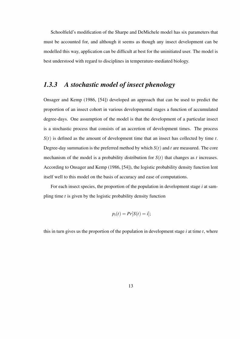
2.2 This is a graph of linear heating and cooling, with the horizontal solid linerepresenting the threshold, and the saw-tooth lines representing the temper-ature, where the area between the two lines, above the threshold, representsthe degree-day accumulation. Here the temperature is measured in ◦C. . . . 22

2.3 An illustration of how the degree-days are calculated with a linear coolingand sinusoidal heating profile. The shaded area represents the degree-dayaccumulation of the current day (or day of interest). The program we usesplits the calculation of degree-days into three sections. The horizontal lineat 12 ◦C represents the development threshold. . . . . . . . . . . . . . . . 23

2.4 This is a graph of sinusoidal heating and cooling, again with the solid linerepresenting the threshold, and the curved dashed line representing the tem-perature. The degree-day accumulation is as it was represented in Fig. 2.2 . 26

2.5 An illustration of degree-day accumulation with a traditional sinusoidalheating and cooling profile. The straight line above the time axis repre-sents the temperature development threshold. The shaded area under thesinusoidal curve and above the threshold represents the degree-day accu-mulation. . . . . . . . . . . . . . . . . . . . . . . . . . . . . . . . . . . . 30

2.6 This figure shows the mixture with sinusoidal heating and linear cooling;the representation of the dashed lines and degree-day accumulations are thesame as those in Figs. 2.2 and 2.4. . . . . . . . . . . . . . . . . . . . . . . 31

2.7 This figure represents traditional sinusoidal heating and cooling when onlythe minimum and maximum are used to construct the sine wave; this figurerepresents the situation where the sine wave is above the threshold at thebeginning of the day. . . . . . . . . . . . . . . . . . . . . . . . . . . . . . 33

2.8 This is the same as Fig. 2.7 with the exception that the sine wave is belowthe threshold when the day begins . . . . . . . . . . . . . . . . . . . . . . 34

2.9 Comparison of degree-day accumulation and estimates for temperaturesrecorded 10 cm above the ground. . . . . . . . . . . . . . . . . . . . . . . 38

3.1 A plot of a simple version of the logistic equation. . . . . . . . . . . . . . . 403.2 A plot of a Richard’s equation, or the generalized logistic function. . . . . . 41

xi

3.3 Comparison of two different forms of the logistic equation. . . . . . . . . . 423.4 Comparison of two logistic equations with different translations in regards

to the x-axis. These are the set of equations in Eq. (3.5). . . . . . . . . . . . 453.5 The plot of G(x), H(x) and their difference, I(x). . . . . . . . . . . . . . . 463.6 A logistic curve to model insects moving into their last life stage. . . . . . . 473.7 A plot of a(x), b(x) and c(x) of equations (3.8). . . . . . . . . . . . . . . . 493.8 The logistic phenology model, exhibiting the different instar proportions.

Note that p1(t) contains the proportion of grasshoppers in instar one andbelow (Dennis and Kemp (1988, [10])). . . . . . . . . . . . . . . . . . . . 50

3.9 Plots of p1(t) when v is varied. . . . . . . . . . . . . . . . . . . . . . . . . 523.10 Plots of the intermediate stage p2(t), as v changes. . . . . . . . . . . . . . . 533.11 Plots of p5(t) as v varies. . . . . . . . . . . . . . . . . . . . . . . . . . . . 543.12 Holding v constant and increasing the a1 and a2 values for the intermediate

probability p2(t). . . . . . . . . . . . . . . . . . . . . . . . . . . . . . . . 553.13 A plot illustrating what happens when v and a1 are held constant and a2 is

allowed to vary. . . . . . . . . . . . . . . . . . . . . . . . . . . . . . . . . 56

4.1 An example of a reflection, where the old simplex is comprised of thepoints xh, xs, and xl . The new simplex is composed of the points xr, xs,and xl . . . . . . . . . . . . . . . . . . . . . . . . . . . . . . . . . . . . . . 62

4.2 An example of an expansion of the simplex. The old simplex is as in Fig.4.1 and the new simplex is xh, xs, and xc. . . . . . . . . . . . . . . . . . . . 63

4.3 An outside contraction of the simplex. The old simplex is as in Fig. 4.1and the new simplex is xh, xs, and xc. . . . . . . . . . . . . . . . . . . . . . 63

4.4 An inside contraction of the simplex. The new simplex and old simplex arethe same as those in the last figure. . . . . . . . . . . . . . . . . . . . . . . 64

4.5 Shrinking of the simplex. The old simplex is the larger of the two triangles. 654.6 A look at the SSE from a vantage point outward from the origin and the

v-axis. The unlabeled axis is the value for the SSE. . . . . . . . . . . . . . 714.7 The surface of an SSE with only three data points, from our mini-model

with parameters a1, and a2 varying with v=1. . . . . . . . . . . . . . . . . 734.8 The surface of an SSE with six data points, again allowing a1 and a2 to

vary while keeping v=1. The surface seems generally more complex thanin Fig. 4.7. The a1 axis is the left axis in this illustration whereas the a2axis is the right axis. The vertical axis is the value of the SSE. . . . . . . . 74

4.9 Here v = 1 and we can see that there are peaks and valleys occurring. . . . . 754.10 In this figure v = 0.5, and we are looking at the surface of SSE. The un-

labeled axis is the value of the SSE. The peaks and valleys seem morepronounced here than in Fig. 4.9. . . . . . . . . . . . . . . . . . . . . . . . 76

xii

Chapter 1

Introduction

1.1 Overview

This chapter gives a discussion of the need for numerical models that allow forecasting of

the timing of insect activity, and a description of some models that have been used. Some

of these are currently being used to predict development rates of insects, or by extension

proportions of a population of insects that are in a particular age class. The rationale for

choosing the logistic phenology model for predicting the occurrence of peak instars for

insect populations is described. The models are then applied to the problem of predicting

age class progression in populations of grasshoppers on the Canadian Prairies. This insect

was chosen because of the very significant damage that can result from its appearance in a

wide range of crops, including recent interest in reducing losses in production of lentils, a

high-value crop in Canada with considerable benefits for economics and health.

This thesis has the objective of producing a model that can improve upon forecasting

methods of pest insects. Also, this thesis strives to provide insights into using a logistic

phenology model when modeling growth of pest insects, especially grasshoppers. By im-

proving upon forecasting methods for pest insects, insecticide usage will be reduced. A

reduction in pesticide usage will produce economic and environmental benefits (Smith and

Holmes (1977, [71],) Gage et al. ( 1982, [16]), [84]).

According to a May 2008 Statistics Canada report, in the last ten years Canadian farm-

ers have harvested an average of 579,400 hectares of lentils per year with an average yield

of 1.51 MT per hectare. This represents an average total production of 710,200 MT of

lentils grown per annum, totalling farm cash receipts of nearly 194 million dollars (CDN)

[73], [13]. This underscores the economic importance of the thesis objective of improving

1

upon forecasting methods of pest insects that influence the development of these crops.

1.2 Insect pest activity and timing

Economic losses caused by herbivorous insect pests in agriculture and forestry are gener-

ally dependent on the timing of insect pest emergence, and subsequent rates of growth and

feeding. Crops have stages that are particularly susceptible to insect attack, and pest con-

trol actions to reduce the activities or abundance of insects must also be timed carefully in

order to be effective and efficient. This is particularly true for vegetation or crop plants that

are susceptible in numerous parts of the cycle of plant growth and development. Lentils

are a good example. The young lentils can be severely damaged by grasshopper feeding,

and in some cases this may result in a need for reseeding, with losses caused by delayed

germination and growth. When the plants begin to mature, grasshoppers may feed on the

reproductive tissue that will produce harvestable yield. Olfert and Slinkard (1999, [56])

found that two-striped grasshoppers (Melanoplus bivitattus) feeding on flowers and devel-

oping pods of lentils in Saskatchewan caused severe losses at very low levels of infestation.

Populations of only 2-3 per meter squared (about one-fifth of the density that is typically

damaging to other crops) resulted in losses of 23% of the pods and 47% of the flowers and

immature pods. Grasshoppers can also degrade the final product by their presence in the

harvested crop, when dead insect parts reduce the quality and value [84]. In the case of

lentils, anticipating the timing and stage of development of the grasshoppers is crucial to

directing control efforts that are effective, and use as little insecticide as possible to reduce

the risk to acceptable levels. Previously, the timing of age class and related damage risk as-

sociated with grasshoppers have been predicted with various approaches to heat summation

(Berry et al.(1995, [3]), Regiert (1968, [65]), Gage et al. (1976, [15]), Mukerji et al. (1976,

[50]), Mukerji et al.(1977, [51]), Lockwood and Lockwood (1991, [43]), Lactin and John-

2

son (1996, [38]), Lactin and Johnson (1996, [39], Lactin and Johnson (1995, [36])). An

understanding of insect timing and developmental progression is key to pest management

strategies, and therefore refinement of predictive models offers benefits for the economics

of pest control, for the environment, and for the quality of the resulting food product. Such

predictive tools would benefit many farmers who grow pulse crops, especially farmers in

Saskatchewan, since they account for 67 percent of lentils produced globally [17].

Insects are dependent on heat from the external environment to emerge from quiescent

stages, and complete their life cycles. Therefore, methods for forecasting insect life his-

tory events and related economic losses have relied mainly on weather data for estimates

of probable insect body temperature and timing. Temperature-based models have become

central to pest management (Randell and Mukerji (1974, [63]), Preuss (1983, [60]),Fisher

(1994, [14]), Hilbert (1995, [22]), Lactin and Johnson (1998, [40], [41]), also see Appendix

A), particularly in temperate zones, because the methods allow more precise anticipation

of the calendar dates and expected magnitude of risk (the probable levels of damage to

crops, in terms of losses in quantity and quality). As noted, such refinements in the power

of prediction are more environmentally sustainable, because pest managers can reduce in-

secticide use if they have access to better information on the timing and geography of the

appearance of susceptible or damaging insect stages. Information is the keystone of sus-

tainable integrated pest management, and this includes general information on pest life

cycles and natural enemies, as well as current information on pest life cycle events, such as

emergence and maturation.

Insect survival, growth and development can occur only over a limited temperature

range. When insect development times (meaning time required to pass from one stage to

the next) are measured at temperature intervals, a “U”-shaped curve of time versus tem-

perature results. This “U”-shaped curve can be seen in Fig. 1.1. If the reciprocals of the

development times are plotted as rates versus temperature, the relationship appears as a

3

curve, shown in Fig 1.3. Empirical and biophysical models describe either the time versus

temperature or the rate versus temperature numerical relationship of insect development.

The rate versus temperature relationship is widely used in models designed to model and/or

predict insect development. The rationale for using the rate versus the temperature relation-

ship to predict insect development times is that the mean daily or total growth rates can be

accumulated under fluctuating temperature environments. Once the accumulation of the

development rates reaches 1.0, the development of the instar (the name for an insect in a

particular immature age class) is complete, and the model can be adapted to predict what

portion of the development of the population cohort is complete. For this reason, models of

development time versus temperature curves are usually used as descriptive tools; however,

they can easily be converted to rate versus temperature models by taking the reciprocal of

development times to yield development rates.

Typically, a measure of heat accumulation known as degree-days is used to gauge de-

velopment rates in pest insects. The concept of degree-days is explained in greater detail

in Chapter 2 of this thesis. It is important to have accurate tools to measure the amount

of degree-days that are “experienced” by the insect and accumulated as successful physi-

ological activity and development. Accurate tools to measure heat accumulation support

better predictions of pest insect development and emergence, and thereby also support more

effective and sustainable pest management. If estimates for heat accumulation and subse-

quently pest emergence are incorrect, even by a few days, for example, it can result in

additional and very significant damage to crops, and may enhance future risk as undetected

pest infestations increase in density or number of locations.

Prediction of heat accumulation (degree-days) may be imprecise, because of sampling

error, for example because of the heterogeneity of the soil and crop environment, or it

may be inaccurate, providing false information of early emergence of a pest problem, or

providing warning too late. Greater accuracy in predicting degree-days is one aim of the

4

Figure 1.1: A curve showing the “U” shape that occurs when development time versustemperature is plotted.

model refinement undertaken in this thesis. With better calculation of degree-days, min-

imization of financial losses incurred by pest managers can be realized, and inefficient

use of pesticide can be prevented. Currently, the “average method”, Eqn. (2.1) described

in Chapter 2 is widely used as a tool to predict insect emergence, including in Alberta

(e.g., Broatch et al. (2006, [4]), Eizenberg et al, (2005, [11])). Degree-days are used

in many places in the US and Canada for pest forecasting and monitoring. For exam-

ple, in Utah, Table 1.1 and Table 1.2 are supplied so farmers can make their own cal-

culations [80]. On the Canadian Prairies, the Insect Pest Monitoring Network (IPMN,

http://www.westernforum.org/IPMNMain.html) uses degree-days as a tool to keep the agri-

culture industry informed of possible risk to crops due to pest insects. This organization

also works with users to conserve natural enemies of these pest species. ( A list of example

5

cases and locations where degree-days are provides and used is listed in appendix A.)

Target Insect Lower Threshold (◦F) Upper Threshold (◦F)Alfalfa weevil 50 87

Armyworm 50 84Codling moth 50 88

Peach twig borer 50 88Peach psylia 41 -

Table 1.1: A partial list of pest insects that occur in Utah and their upper and lower temper-ature development thresholds.

Target Insect DD Min DD MaxBlack pineleaf scale 1068 -

Cankerworm 148 290Lilac root weevil 500 950

Locust borer 2271 2805

Table 1.2: A partial list of degree-day (DD) accumulations for selected landscape pests thatoccur in Utah. DD Min is the earliest time for appearance and DD Max is the latest timefor appearance.

The average method tends to underestimate the amount of degree-days that are actually

accumulated. Better or improved degree-day accumulators, coupled with a suitable in-

sect life cycle model, are likely to achieve greater accuracy and precision when predicting

grasshopper pest emergence, and therefore support more informed efficient pest manage-

ment( Johnson (1989, [30]), Logan (1988, [45]), Pannell (1991, [58]), Quinn et al. (1993,

[62]), Onsager (2000, [55]). tactics.

6

1.2.1 A brief description of the grasshopper life cycle

During the two weeks following mating, the female grasshopper hunts for an appropriate

site to deposit her eggs. Once she selects a site she bores a hole and deposits eggs. She

then deposits a foamy secretion over the eggs that hardens them to form an egg pod.

Once the eggs are laid embryological development beings and continues until environ-

mental conditions become unfavourable in the fall and will resume in the spring as the soil

temperature rises. Newly hatched grasshoppers, or nymphs, are approximately 5 mm (0.2

of an inch) in length. Nymph are similar in appearance to adults, however nymphs are

smaller than adults and also do not have wings.

It will take approximately 35 to 50 days for the nymphs to go through the 5 nymphal

or instar (immature grasshopper) stages before becoming a mature grasshopper. Generally

the adult females are slightly larger than the males (Johnson (2008, [29]), [18]).

1.3 Insect development models and methods

1.3.1 Earlier rate models

Finding an appropriate model to utilize the improved degree-day accumulators is important

to devise optimal pest management strategies. Here I outline some historical models as

background for the choice of approach used in this thesis.

Janisch’s (1925, 1932, [27, 28]) inverted symmetric and inverted asymmetric catenaries

are empirical models [83] used to describe development time as a function of temperature.

The catenaries are inverted to give development in units per day. Looking at Eqn. (1.1), the

inverted catenary will be symmetric if b1 = b2; otherwise the function will be asymmetric,

as seen in Fig. 1.2. The following equation is the generalized inverted cantenary of Janisch

7

:1τ

=2a

b(T−Tm)1 +b(Tm−T )

2

. (1.1)

Here 1τ is the development rate at temperature T (in ◦C). Tm is the temperature where τ is a

Figure 1.2: The solid line represents the situation where b1 6= b2 whereas the dashed lineshows a symmetric inverted catenary. These curves are plotted with contrived parametersfor illustrative purposes and do not relate to any specific insect.

minimum (and development rate is maximal, so in that sense Tm is optimum). Also a is the

measured rate at Tm, and b expresses the rate of decline in growth as T diverges from Tm.

Janisch’s equation has been used with some degree of success (Rathjen (1939, [64]),

Huffaker (1944, [23]), and Quednav (1957, [61])). Some problems associated with it are

that it can result in improper fits to data, and can run into computational difficulties (Mes-

senger and Flitters (1958, [48])). The resulting incorrect fitted values can result from bias or

from incorrect parameter estimates given by software that calculates the parameters based

8

on nonlinear regression.

Another equation that describes development rates as a function of temperature is the

logistic equation. The logistic equation as used by Davidson (1944, [8]) is

1y

=K

1+ e(a−bx) , (1.2)

where 1/y represents the reciprocal of the time required for complete development to be

achieved at a given temperature x. K, a and b are constants. Davidson’s paper (1942, [7])

does not attribute any biological meaning to these constants.

Davidson (1942, [7]) was one of the first to use a logistic equation to describe insect

development rates as a function of temperature. Davidson’s treatment with the logistic

equation has been widely used (Guppy and Mukerji (1974, [19]), Taylor and Harcourt

(1978, [75]), Thomas (1980, [77]), Lamb and Laschiavo (1981, [42])), and Davidson used

this logistic equation as early as the 1940s.

1.3.2 More contemporary models

A modified sigmoid equation was used by Stinner et al. (1974, [74]) to describe the effects

of temperature on insect development rates. The result of Stinner’s work led to a develop-

ment curve similar to that of the logistic equation, however the fitted development rate in

Stinner’s treatment would drop off after the optimum temperature had been reached [74].

Logan et al. (1976, [44]) were able to improve upon Stinner’s sigmoid curve by creating

a combination of two exponential equations to describe intermediate and high tempera-

ture influences on development rates. An additional advantage of Logan’s model is that its

9

parameters have biological meaning. Logan’s model equation is:

r(T ) = Ψ(eρT − e(ρTmax− (Tmax−T )∆ )). (1.3)

The parameters of Logan’s model have the following meanings: Ψ is a directly measurable

rate of a temperature-dependent physiological process at some base temperature; ρ can be

interpreted as a composite Q101 value for critical enzyme-catalyzed biochemical reactions;

Tmax is the thermal maximum (the temperature at which life processes can no longer be

sustained except for short durations of time); and ∆ is the temperature range at which

thermally induced breakdown becomes the overriding factor.

The Logan model cannot estimate a low temperature developmental threshold because

the design of the Logan equation will not allow the rate curve to intersect the temperature

axis (or the abscissa) at suboptimal temperatures. The low temperature asymptote of the

Logan model is 0. Lactin et al. (1995, [37]) produced a modified version of the Logan

model which eliminates one parameter and introduces another. Their model is exhibited

below:

r(T ) = eρT − e(ρTmax− (Tmax−T )∆ ) +λ. (1.4)

The difference between the Lactin and Johnson model and Logan’s model is that Ψ

is removed and now there is a new parameter, λ, which allows the development curve to

intersect the temperature axis at suboptimal temperatures and thus allows estimation of a

lower developmental threshold. Thus, this model can take into account intermediate and

high temperatures, and also accounts for growth at lower temperatures. A comparison of

the Logan model and Lactin and Johnson model can be seen in Fig. (1.3).

1The temperature coefficient Q10 represents the factor by which the rate of a reaction increases for every10-degree rise in temperature (◦C).

10

Figure 1.3: A plot comparing the Lactin model with the Logan growth model.

A widely cited growth model was developed by Sharpe and DeMichele (1977, [68]) that

describes reaction kinetics of poikilotherm2 development. Sharpe and DeMichele (1977,

[68]) were able to develop a model based on work done by Eyring (1935, [12]), Johnson

and Lewis (1946, [31]), and Hultin (1955, [25]). The model that resulted is a complex

biophysical model, and has the ability to illustrate nonlinear responses in development rates

at both high and low temperatures, along with the standard linear response at intermediate

temperatures. The complexity of the model can hinder users who are not familiar with the

pitfalls of nonlinear parameter estimation. This makes the model somewhat inaccessible to

the general user. Schoolfield at al.(1981, [67]) modified the form of the original equation in

order to make the model more accessible to the general user. The Schoolfield modification

2A poikilotherm is a plant or animal whose internal temperature varies along with that of the ambientenvironmental temperature.

11

to the Sharpe and DeMichele model is listed as follows3:

A =RHO25298.15

expHA ·T −HA ·298.15

R ·298.15 ·T (1.5)

B = 1+ expHL ·T −HL ·T H

R ·T L ·T + expHH ·T −HH ·T H

R ·T H ·T (1.6)

r(T ) =AB

(1.7)

The following list explains the variables of the prior equations:

r(T )= the mean development rate (per day) at temperature T (degrees Kelvin);

R= the universal gas constant (8.314472 J K−1 mol−1);

RHO25 = the development rate at 25 degrees Celsius assuming no enzyme activation;

HA= enthalpy of activation of the reaction that is catalyzed by a rate-controlling

enzyme;

T L= the temperature at which the rate controlling enzyme is half active and half low

temperature inactive;

HL= change in enthalpy associated with low temperature inactivation of the enzyme

(in degrees Kelvin);

T H= the temperature at which the rate-controlling enzyme is half active and half

high temperature inactive (in degrees Kelvin);

HH= change in the enthalpy associated with the high temperature inactivation of the

enzyme.

3Note that the equations for A and B represent the numerator and denominator for the rate equation,respectively.

12

Schoolfield’s modification of the Sharpe and DeMichele model has six parameters that

must be accounted for, and although it seems as though any insect development can be

modelled this way, application can be difficult at best for the uninitiated user. The model is

best understood with regard to disciplines in temperature-mediated biology.

1.3.3 A stochastic model of insect phenology

Onsager and Kemp (1986, [54]) developed an approach that can be used to predict the

proportion of an insect cohort in various developmental stages a function of accumulated

degree-days. One assumption of the model is that the development of a particular insect

is a stochastic process that consists of an accretion of development times. The process

S(t) is defined as the amount of development time that an insect has collected by time t.

Degree-day summation is the preferred method by which S(t) and t are measured. The core

mechanism of the model is a probability distribution for S(t) that changes as t increases.

According to Onsager and Kemp (1986, [54]), the logistic probability density function lent

itself well to this model on the basis of accuracy and ease of computations.

For each insect species, the proportion of the population in development stage i at sam-

pling time t is given by the logistic probability density function

pi(t) = Pr[S(t) = i];

this in turn gives us the proportion of the population in development stage i at time t, where

13

the values for i = 1, . . . ,r.

p1(t) =[

1+ exp(−(a1− t)√

vt

)]−1

, i = 1;

pi(t) =[

1+ exp(−(ai− t)√

vt

)]−1

−[

1+ exp(−(ai−1− t)√

vt

)]−1

, i = 2, . . . ,r−1;

pr(t) = 1−[

1+ exp(−(ar−1− t)√

vt

)]−1

, i = r, (1.8)

where t is the degree-day accumulation at a particular collection date, ai is the amount of

development needed to complete the ith phenology stage, v is a positive constant, r is the

final phenological stage, and S(t) is the amount of development an insect has accumulated

at t. This model has attributes that will be discussed further in this thesis since it will be

the model that I am primarily working with.

1.4 Choosing a model

After consideration of the attributes of the various models described above, the model that

we chose to work with was the stochastic phenology model presented by Onsager and

Kemp (1986, [54]). One factor weighing in this decision was the availability of field data

as it pertains to instar counts for different geographic locations for different days throughout

a particular year, for different years, and for different species [85]. Another reason for this

choice is the ease of constructing degree-day integrators to take in large amounts of weather

data and calculate degree-day accumulations for various sites for particular days on which

grasshopper population data was taken. Grasshopper counts and accumulated degree-days

provide enough information to solve for the parameters of the logistic density function

proposed by Onager and Kemp (1986, [54]).

The existence of a basis for valid comparison is another reason we chose the stochastic

14

phenology model. Onsager and Kemp (1986, [54]) calculated parameters for six different

species of grasshoppers in the Montana area for years 1975 and 1976. We have additional

exemplar data and methodologies for solving the six parameters in the logistic density

distribution, for our region and nearby regions. Onsager and Kemp (1986, [54]) use a non-

linear optimization technique known as the Nelder-Mead simplex algorithm. This method

is used to find the parameters of the stochastic phenology model they propose, and can also

be used to fit these parameters to sets of data that are available.

1.5 Thesis outline

This thesis examines the use of a stochastic phenology model as a tool for better predicting

the emergence and timing of grasshopper life cycles. Chapter 2 discusses the concept of

a degree-day and methodologies used to calculate degree-days. Chapter 3 introduces the

setup for finding the parameters of the logistic probability distribution. Chapter 4 discusses

the fit and validation of the nonlinear regression that we are applying and some mathemat-

ical aspects of our optimization problem. Chapter 5 presents field validation, application,

and future work and prospects that can be accomplished with this model.

15

Chapter 2

Degree-days

2.1 Chapter overview

This chapter looks at some historical methods of calculating degree-days, and explains how

some of these methods are imprecise. Also, within this chapter I explain the degree-day

accumulation methods that I have developed that take into account temporal aspects of

heating and cooling that are occurring within a day. At the end of this chapter there is a

comparison of how my accumulators compare with each other, and how they compare to

“true degree-day accumulation”.

Another aim of this chapter is to familiarize the reader with the concepts of degree-days

and accumulated degree-day, since subsequent chapters and their analyses of the logistic

phenology model require and understanding of these concepts.

2.2 Physiological time and degree-days

The main component that drives developmental rates of many exothermic organisms is

environmental temperature. These temperature-dependent organisms require adequate heat

to develop from one point in their life stage to another. Physiological time is the measure of

the time passage adjusted for the amount of heat available for the organism to complete life

stages. Theoretically, physiological time provides a common reference for the development

of organisms. If organisms were completely temperature-dependent, then physiological

time would remain a constant for a particular temperature. However, organisms are not

completely temperature-dependent, but a large component of their development is based

on heat accumulation; thus, estimates for approximate development times can be made.

16

These approximations of physiological time are often expressed in units called degree-days

(Baskerville and Emin (1969, [2]), Higley et al. (1986, [21]), [79]).

Figure 2.1: The black area represents the degree-day accumulation. The figure is takenfrom the site located in the bibliography [79].

Sometimes called heat units, degree-days are the accumulated product of time and tem-

perature above a particular developmental threshold and below a maximum threshold for an

organism. The lower developmental threshold for an organism is the temperature at which

development stops. Estimates of upper developmental thresholds also exist for organisms;

however, in our treatment of calculating degree-day accumulations for grasshoppers on the

Canadian Prairies, these upper thresholds are not met and therefore excluded from our dis-

cussion. One degree-day is one day (24 hours) with the temperature one degree above the

lower developmental threshold. For example, if our developmental threshold is 12 ◦C and

our temperature remains at 13 ◦C for 24 hours, then one degree-day is accumulated.

17

2.3 Methods for calculating degree-days

There are several methods for calculating degree-days. One of the most rudimentary forms

for calculating degree-days is done using averages:

DD = max(

0,Tmax +Tmin

2−Tbase

). (2.1)

Here DD is the degree-days accumulation for the day, Tmax is the maximum temperature for

that day, Tmin is the minimum temperature for that day, and Tbase is the lower developmental

threshold. If Tmax+Tmin2 −Tbase is negative, then the accumulation for that particular day is

simply set to zero, as a negative accumulation of degree-days would incorrectly imply that

growth could be reversed, which is biologically impossible.

This method can have problems with its accuracy of calculating degree-days. It does not

take into account the length of heating and cooling periods throughout a day. This method

can theoretically overestimate degree-day accumulations when there is a day that has a

long period of cool temperatures. For instance, if the temperature is high at the beginning

of the day and begins to fall rapidly to a lower temperature that is maintained for the bulk

of the day, then degree-days will be overestimated. This method can underestimate degree-

day accumulation as well. If there is a particular day where the temperature increases

rapidly from a low temperature and maintains a relatively high temperature, the degree day

accumulation will be underestimated. In all the cases we tested, this method underestimates

the degree-day accumulation.

Depending on the temperature data available, one can use a variety of methods for

increasing the precision of calculating degree-days. For example, if a researcher had tem-

perature data recorded every minute, then a rectangular method for calculating degree days

would be entirely appropriate. In the rectangular method1, the recorded temperature minus

1The rectangular method is just a Riemann sum. In this case, we take the height of the rectangle to be the

18

the temperature threshold is the height of the rectangle we are using to calculate the degree-

days. If the temperature is below the threshold, the area of the rectangle is zero. The length

of the rectangle is the amount of time we are measuring this temperature for. In order to

get the amount of heat accumulated in degree-days, we need to divide the rectangle by the

fraction of a day that the time occupies. In such a case the degree-day accumulation for

one minute would be

DD = max(

0,T −Tbase

1440

). (2.2)

Any differences of T −Tbase that are negative would be set to zero, and the total degree-

days accumulated for the particular day would be the sum of the degree-days for the 1440

observations (minutes per day). It is not typical or necessary that a researcher would have

1-minute temperature intervals available for a multitude of locations, so this method is

somewhat impractical. More realistically, a researcher would have most major locations

with hourly temperature observations, and the rest of the sites with just daily maximum

and minimum temperatures available.

Another popular method of calculating degree-days is to fit a sine wave to a particular

day. This method was popularized by Allen (1976, [1]) and only requires that a daily

temperature maximum and minimum be supplied. From the particular day’s maximum

and minimum, a sine wave is constructed to fit these two points (see Figs. 2.6 and 2.7).

The degree-day accumulation using Allen’s modified sine wave is simply the area above

the development threshold and the area below the fitted sinusoidal wave. This area can be

easily computed by integrating the sine wave and finding the area underneath it, and then

subtracting the area below the developmental threshold. This method will be explained in

greater detail as it is one of the methods employed in our model for finding degree-day

accumulations. This method is widely used (Lysyk (2007), [46]).

recorded temperature minus the temperature threshold. Since this measure of height occurs at the start of therectangle being constructed, we have a left Riemann sum.

19

Some other methods for finding degree-day accumulation are the linear heating and

cooling model (Fig. 2.2), the sinusoidal heating and cooling model (Fig. 2.4), and the si-

nusoidal heating mixed with the linear cooling model (Fig. 2.6). With these three models

we require the the prior day’s maximum, the current day’s minimum and maximum respec-

tively, and the next day’s projected minimum (or recorded minimum if we are using prior

data).

2.4 Degree-day accumulators used in the model

The degree-day accumulators that end-users have a choice of utilizing in our constructed

model are the traditional sinusoidal method, the linear heating and linear cooling method,

the sinusoidal heating and cooling method, and the linear cooling and sinusoidal heating

method. The traditional sinusoidal method only requires the maximum and minimum tem-

peratures respectively to estimate the degree-day accumulation for a particular day. The

other three accumulators have a temporal aspect that must be accounted for, because they

not only require specific temperature information, but also require when these temperatures

are occurring.

To capture the temporal aspect of the three time-dependent integrators, a subroutine

called SRLOCAT [26] was employed. This subroutine requires the end user to input the

particular latitude and longitude for their region of interest. SRLOCAT calculates the sun-

rise and sunset for a particular day of a year, at that location. The sunrise and sunset give

us an idea of how heating and cooling are occurring throughout a day at a specific location.

For our purposes, we chose the heating portion of a particular day to begin at sunrise. The

beginning of the cooling period is taken as two hours after solar noon [5]. As for solar

noon, it was estimated as the midpoint of the time of sunrise and the time of sunset.

20

2.4.1 Linear heating and cooling

When estimating linear heating and cooling for a particular day, the start of that particular

day is taken to be 0:00 hrs and the end of the day is 24:00 hrs. Once the boundaries of time

for the day are established, the process for calculating the degree-day accumulation for

that day begins. In the program for calculating linear heating and cooling, there are some

assumptions to consider: cooling takes place from yesterday’s maximum until today’s min-

imum; heating takes place from today’s minimum to today’s maximum, and cooling takes

place from today’s maximum to tomorrow’s minimum. Given these three asssumptions the

degree-day calculation can be split into three sections. The first and the last sections deal

with the cooling that takes place during the day, and the second or middle section deals

with the heating that takes place for that particular day.

When calculating the degree-day accumulation for the first section (the first cooling

section) we have to consider different scenarios. The first and simplest scenario is the

temperature profile line falls below the threshold line at the beginning of the day. If this

is the case, the degree-day accumulation for that particular portion of the day is zero. The

second case occurs when the temperature at the beginning of the day is above the threshold,

and the temperature profile cools to a value below the threshold temperature. In this case

the degree-day accumulation is

DD1 =(x1)(b−Ta)

48. (2.3)

In the above equation, DD1 is the amount of degree-day accumulation, x1 is where the

temperature profile intersects the threshold, b is where the temperature profile intersects

the temperature axis at the beginning of the day, and Ta is the temperature below which

21

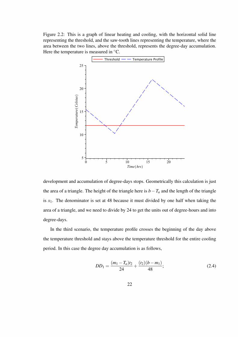
Figure 2.2: This is a graph of linear heating and cooling, with the horizontal solid linerepresenting the threshold, and the saw-tooth lines representing the temperature, where thearea between the two lines, above the threshold, represents the degree-day accumulation.Here the temperature is measured in ◦C.

development and accumulation of degree-days stops. Geometrically this calculation is just

the area of a triangle. The height of the triangle here is b−Ta and the length of the triangle

is x1. The denominator is set at 48 because it must divided by one half when taking the

area of a triangle, and we need to divide by 24 to get the units out of degree-hours and into

degree-days.

In the third scenario, the temperature profile crosses the beginning of the day above

the temperature threshold and stays above the temperature threshold for the entire cooling

period. In this case the degree day accumulation is as follows,

DD1 =(m1−Ta)t2

24+

(t2)(b−m1)48

; (2.4)

22

Figure 2.3: An illustration of how the degree-days are calculated with a linear cooling andsinusoidal heating profile. The shaded area represents the degree-day accumulation of thecurrent day (or day of interest). The program we use splits the calculation of degree-daysinto three sections. The horizontal line at 12 ◦C represents the development threshold.

where m1 is the minimum temperature that occurs at time t2. Also, b, Ta and DD1 are as

previously defined. In this case we have a triangle as before, which has a height of b−m1

and a length of t2. We also have an additional rectangle that needs to be accounted for and

the dimensions of this particular rectangle are m1−Ta, which is the height of the rectangle,

and t2, the length of the rectangle. Again, in this scenario, we must divide the area of the

rectangle by 24 to get out of degree-hour units and into degree-day units.

In the second section of the computation of our degree-days, for one day we are dealing

with the temperature profile where heating is occurring. Much like in the first section we

have different scenarios. In the first scenario, if the maximum for the particular day is less

than the threshold, there will be no degree-day accumulations for either section 2 or 3,

because we are under the assumption that the third section of the temperature profile is a

cooling section. Thus, if our maximum for this day is lower than our threshold, then the

minimum for the next day will also be below the threshold as the temperature profile cools

23

from today’s maximum until tomorrow’s minimum. Thus the whole temperature profile for

sections 2 and 3 lies below the threshold and therefore no degree-day accumulation occurs.

In another scenario for the second section of the temperature profile, we have today’s

maximum temperature higher than the threshold, and today’s minimum less than the thresh-

old. In this case we have our degree-day accumulation as

DD2 =(M2−Ta)(r2− x2)

48, (2.5)

where DD2 is the amount of degree-day accumulation that occurs in the heating section

of the day, r2 is the period of time over which the heating period extends, x2 is where

the temperature profile intersects the threshold line, M2 is the maximum temperature for

the day and Ta is defined as it was previously. Geometrically we are again calculating the

area of a triangle where M2−Ta is the height of our particular triangle. The length of this

triangle is r2− x2. We calculate the area of this triangle and divide by 24 to give us our

associated degree-days for section two.

In the third scenario, both the daily maximum and minimum temperature lie above the

threshold. Here the degree day accumulation for section two is:

DD2 =r2(m1−Ta)

24+

(M2−m1)r2

48. (2.6)

Here all the variables are as previously defined, for the scenario is much like the one en-

countered in section one, where the degree-day accumulation is equal to the area of a

rectangle plus that of a triangle. Here our rectangle has a height of m1−Ta and the length

of the rectangle is r2. The triangle has a height of M2−m1 and a length of r2.

In the third section, our temperature profile is in another cooling phase. We have already

covered the scenario where no accumulation occurs. One of the other scenarios is where

24

the temperature profile does not intersect the threshold before the end of the day. The

degree-day accumulation is

DD3 =(M2−b1)r4

48+

(b1−Ta)r4

24, (2.7)

where DD3 is the accumulation for the third section of the FORTRAN program. Here, r4 is

the amount of time contained in the final cooling period for the day, b1 is the temperature at

the end of the day, and all other variables are as previously defined. r4 is the length of both

the triangle and rectangle, M2−b1 is the height of the triangle, and b1−Ta is the height of

the rectangle. The accumulated degree-days are again the area of the rectangle and triangle.

In the final scenario, our temperature profile crosses the threshold before the day is

complete. The associated degree-day accumulation for this final section is computed as

DD3 =(M2−Ta)x3

48. (2.8)

The variables are all defined as before and the only new variable is x3, which is the time

at which the temperature profile crosses the threshold. This equation is just the area of a

triangle with height M2−Ta and the length x3. Again the area must be divided by 24 in

order to get the proper units of degree-days, and the other factor of 2 in the denominator

comes as the result of finding the area of a triangle.

2.4.2 Sinusoidal heating and cooling

In this section we explore in detail how the degree-day accumulation works when our tem-

perature profile is simulated by sinusoidal curves, rather than lines, as was the case in the

previous subsection of this chapter. In this case, we again have three assumptions about the

25

heating and cooling sections of a day. Here we assume that the temperatures decrease from

yesterday’s maximum until today’s minimum, and this is the first section of cooling in our

day, as well as the first section where degree-day accumulation is computed in our FOR-

TRAN program. In the second section, where the day’s heating is occurring, we assume

that the temperature rises from today’s minimum temperature until today’s maximum tem-

perature. Finally, in the third section we assume that the temperature profile shows cooling

from today’s maximum temperature until tomorrow’s minimum temperature.

Figure 2.4: This is a graph of sinusoidal heating and cooling, again with the solid linerepresenting the threshold, and the curved dashed line representing the temperature. Thedegree-day accumulation is as it was represented in Fig. 2.2

In the first section, if yesterday’s maximum temperature is below the threshold, then

the degree-day accumulation for the first section is set to zero and the program proceeds.

If yesterday’s maximum temperature is above the threshold, then we have two possible

situations.

26

In the first situation the temperature profile will intersect the threshold before the day’s

temperature minimum is reached. In this case the degree-day accumulation will be

DD1 =1

24

(Z t1

0

(Asin

((t + s1)(2π)

p1− 3π

2

)+B

)dt

)− Ta · t1

24. (2.9)

In this equation the variable t1 is the time at which the temperature profile intersects the

temperature threshold, A is the amplitude of the sine wave, s1 is the amount of time that

elapsed from yesterday’s maximum until the beginning of today, p1 is the period of the

sine wave, Ta is the temperature threshold, DD1 is the amount of degree-day accumulation

for this portion of the day, and B is the average of yesterday’s maximum temperature and

today’s minimum temperature. Also note that we are integrating over t (time), hence the

differential dt. Also, we are subtracting a rectangular area which is the area below the

threshold that is encapsulated by the integral. Notice as well that we are dividing the whole

expression by 24 in order to translate the units of degree-hours into degree-days. This is

done for Eqs. 2.9 through 2.14.

In the previous scenario, the temperature profile does not intersect the temperature

threshold; in this case, the integral is the same as the above with the exception that t1 is

now t2, the time at which today’s minimum occurs. The formula for the degree-day accu-

mulation is as follows:

DD1 =1

24

(Z t2

0

(Asin

((t + s1)(2π)

p1− 3π

2

)+B

)dt

)− Ta · t2

24. (2.10)

In sections two and three of the code, we will get zero degree-day accumulation if

today’s maximum falls below the threshold temperature. This is analogous to the situation

that occurred when the temperature profile was modelled by linear heating and cooling.

With that knowledge, there are two other scenarios that can occur in section two.

27

One particular scenario occurs when our temperature profile is initially below the tem-

perature threshold and then crosses the temperature threshold before the day’s maximum

temperature is reached. In this case, the degree-day accumulation is calculated as

DD2 =1

24

(Z t3

x2

(A2 sin

((t− t2)(2π)

p2− π

2

)+B2

)dt

)− Ta · (t3− x2)

24. (2.11)

The only new variables here are DD2, which is the degree-day accumulation for the second

section of the day. x2 is the time at which the temperature profile intersects the temperature

threshold, t3 is when today’s maximum occurs, A2 is the amplitude of our sine wave for

this particular temperature profile, p2 is the period of the sine wave for this section of the

day, and B2 is the average of today’s minimum and maximum temperatures. Here, t2 shifts

the profile in order to have the sine wave in the proper position. Again we are integrating

with respect to t, which represents time.

In the other scenario for section two, we can have the temperature profile completely

above the temperature threshold, which changes the limits of integration, and subsequently

changes how we calculate the degree-day accumulations for this section of the day. The

integral for this case is:

DD2 =1

24

(Z t3

t2

(A2 sin

((t− t2)(2π)

p2− π

2

)+B2

)dt

)− Ta · (t3− t2)

24. (2.12)

The only change from the prior equation is the lower limit of the integral is now t2

rather than x2.

In the final section for the day, we again have two scenarios other than the scenario

where there is no degree-day accumulation. If the temperature profile does not cross the

28

threshold by the end of the day, our calculation for degree-days is:

DD3 =1

24

(Z 24

t3

(A3 sin

((t− t3)(2π)

p3+

π2

)+B3

)dt

)− Ta · (24− t3)

24. (2.13)

The variable DD3 is the amount of degree-day accumulation for this section of the day,

A3 is the amplitude of the sine wave for this portion of the temperature profile, B3 is the

average of today’s maximum with tomorrow’s minimum, p3 is the period of the sine wave

constructed for this portion of the day, and t3 is the time at which today’s maximum occurs

and is also the amount the sine wave is shifted in order for it to be in its proper location.

The upper limit of the integral is 24, which is the amount of time accumulated at the end of

the day in hours. Notice here the rectangular region which we are subtracting has a length

of 24− t3 and a height of Ta.

The final scenario for the final section is when the temperature profile intersects the

temperature threshold before the end of the day. The only difference between this calcu-

lation for degree-days and the other scenario in this final section is that the the upper limit

of the integration is x3, the time at which the temperature profile intersects the temperature

threshold. The corresponding calculation for the accumulated degree-days for this section

is:

DD3 =1

24

(Z x3

t3

(A3 sin

((t− t3)(2π)

p3+

π2

)+B3

)dt

)− Ta · (x3− t3)

24. (2.14)

29

Figure 2.5: An illustration of degree-day accumulation with a traditional sinusoidal heatingand cooling profile. The straight line above the time axis represents the temperature devel-opment threshold. The shaded area under the sinusoidal curve and above the thresholdrepresents the degree-day accumulation.

2.4.3 Sinusoidal heating and linear cooling

In the sinusoidal heating and linear cooling model of daily temperature, we have a mixture

of the all-linear temperature profile and the all-sinusoidal temperature profile. This method

is basically a cut-and-paste version of the other two methods. Sections 1 and 3 of the linear

cooling are exactly the same as those used in the linear heating and cooling subroutine for

finding degree-day accumulations. Also in section 2 of the subroutine, the methodology

for finding the accumulated degree-days is exactly the same as in section 2 of the purely

sinusoidal temperature profile model. Thus the details are exactly as those found above and

therefore omitted from discussion. Figure 2.4 shows what the temperature profile would

30

look like for a sinusoidal heating and linear cooling model.

Figure 2.6: This figure shows the mixture with sinusoidal heating and linear cooling; therepresentation of the dashed lines and degree-day accumulations are the same as those inFigs. 2.2 and 2.4.

2.4.4 Traditional sinusoidal method

In this model of the temperature profile, there is no temporal dependence, so all that is

required is the maximum temperature and the minimum temperature of the day in order to

construct the sinusoidal wave.

In this case the calculations for the degree-day accumulations are fairly straightforward.

There are four cases that can occur when calculating the degree-day accumulation. The first

case is where the maximum for the day is less than the temperature threshold, in which case

the degree-day accumulation for the day is zero. Another case is where the whole sine wave

31

is above the threshold, and the degree day accumulation in this case is:

DD1 =Z 1

0(Asin(2πt)+B)dt−Ta. (2.15)

Here A is the amplitude of the sine wave, B is the average of the minimum and maximum

of the sine wave, and Ta is the temperature threshold at which growth stops. Notice that

in this case there is no denominator as in other cases, because the units here are already

in degree-days whereas in other subroutines the accumulations were in degree-hours based

on the temporal variation taken into account.

Another case that occurs can be viewed in Fig. 2.7, where the minimum temperature

falls below the threshold during the day, but does so after the start of the day. The degree-

day accumulation is as below:

DD1 =Z t1

0(Asin(2πt)+B)dt +

Z 1

t2(Asin(2πt)+B)dt−Ta · t1−Ta · (1− t2). (2.16)

All the variables are the same as in Eqn. (2.15) and the new variables are t1 and t2. Here,

t1 is where the temperature profile crosses the threshold the first time; subsequently, t2 is

where the profile crosses the threshold the second time.

The final method for calculating the degree-day accumulation for the traditional sinu-

soidal wave occurs when we get a temperature profile as in Fig. 2.8. The integration for the

degree day accumulation is

DD1 = 2Z 1

4

t1(Asin(2πt)+B)dt−2Ta · (1

4− t1). (2.17)

In this case, we use the fact that the sinusoidal wave is symmetric around its peak, which

occurs at 14 day, or π

2 days if the day has the length of 2π. In order to get the degree-day

accumulation, we integrate from when the temperature profile first crosses the threshold

32

(t1) to where the maximum of the sine wave occurs (14), and multiply the whole integral by

two in order to capture all of the area under the curve. In order to remove the area caught

by the integral that is below the threshold, we must subtract 2Ta · (14 − t1), which is the area

of rectangle.

Figure 2.7: This figure represents traditional sinusoidal heating and cooling when onlythe minimum and maximum are used to construct the sine wave; this figure represents thesituation where the sine wave is above the threshold at the beginning of the day.

33

Figure 2.8: This is the same as Fig. 2.7 with the exception that the sine wave is below thethreshold when the day begins

2.5 Comparison of accumulators

For the month of October and up to and including November 6th, 2008, temperatures were

recorded at the University of Lethbridge. One of the temperature recording devices was

positioned in the soil at a depth of 5cm. The other temperature recording device was posi-

tioned 10cm above the ground. Both devices recorded temperature in 10-minute intervals.

Such short intervals of measurement allowed observation of temperature fluctuation at this

specific time of year, and also allowed us to calculate degree-days with a better precision

as discussed earlier in this chapter.

Turning attention to Fig. 2.9, the plot linheat is the degree-day accumulation for the

34

linear heating and linear cooling accumulator, linsin is the degree-day accumulation for

the sinusoidal heating and linear cooling model, sineheat is accumulations produced by

sinusoidal heating and cooling that has a temporal dependence, and the traditional sine fit

is the accumulator that models temperature based purely on the maximum and minimum

temperatures for a day. As a general rule, the linear heating and cooling method always has

the lowest accumulation, followed by the mixture of linear heating and cooling, whereas

the traditional sinusoidal fit and sineheat have the highest degree-day accumulations and

are very close in the values that they produce for the total degree-day accumulations.

To test the general rule above, heat accumulation was tracked at Onefour for the year

2000. The temperature was measured at 2 meters above the ground, as is consistent with

most Canadian weather stations. The degree-day accumulation estimated by each accu-

mulator is listed in the table below. These values are tested against a rectangular method

of calculating degree-days for each hour, since hourly weather data was available for the

Onefour site. The subsequent relative error was then calculated for each degree-day accu-

mulator compared to the rectangular accumulation method. The rectangular method was

used as basis for the measured accumulation or “true degree-days.” Tables for the Univer-

sity of Lethbridge sites and the Onefour site are below.

35

air 10 cm Degree-days (◦C) relative error (percent)measured accumulation 39.24 -

linheat 35.17 −10.36sineheat 41.24 5.1

linsin 37.55 −4.30traditional fit sine wave 40.25 2.57

Table 2.1: Degree-day accumulations at the University of Lethbridge, at a height of 10cm,in the autumn of 2008.

soil 5 cm Degree-days (◦C) relative error (percent)measured accumulation 14.42 −

linheat 15.34 6.09sineheat 17.228 19.47

linsin 16.4497 14.08traditional fit sine wave 17.561 21.78

Table 2.2: Degree-day accumulations at the University of Lethbridge at a depth of 5cm, inthe autumn of 2008.

Air 2 m Degree-days (◦C) relative error (percent)measured accumulation 912.65 −

linheat 889.29 −2.56sineheat 957.18 4.88

linsin 909.40 −0.36traditional fit sine wave 967.67 6.02

Table 2.3: Degree-day accumulation at the Onefour weather station for the year 2000.

36

The relative error of the accumulators is much lower in general for the Onefour data sets

than those taken at the University of Lethbridge. One reason for the lower relative error in

the Onefour data set is that every day during that year was sampled, and therefore we had a

relatively large denominator when comparing relative errors as opposed to having smaller

denominators for relative error in the University of Lethbridge sample data. Also, with

more sampling points for the Onefour data, extreme fluctuations in accumulation or non-

accumulation ought to average out, giving a smaller variance of relative errors for the larger

data set. The relative error can also be a function of the time of the year at which we were

observing the degree-day accumulations. Over the summer months, Onefour would have

long periods of stable weather. October, by contrast, can have large fluctuations in degree-

day accumulation as the temperature profiles are transitioning from summer to winter.

The range of the relative errors for the Onefour data is from -2.56 percent to 6.02

percent; therefore any degree-day accumulator chosen in the model should give a good

approximation of the heat accumulation that is occurring in a specific region. As more in-

formation about grasshopper locations becomes available, the model will be adjustable by

the end users’ requirements for heat accumulation. For example, a user of the model may

wish to use linear heating and cooling, because it may better model what is going on in a

certain type of soil or terrain. Also, users of the program may opt to go with the sinusoidal

heating and cooling model degree-day accumulator or the traditional sinusoidal accumula-

tor. Both of these accumulators tend to overestimate the degree-day accumulation, but this

can be beneficial in some scenarios, such as in cases where a particular grasshopper species

is able to bask, and thereby increase the amount of heat they are accumulating.

37

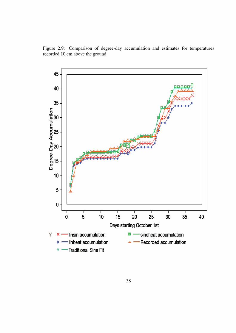
Figure 2.9: Comparison of degree-day accumulation and estimates for temperaturesrecorded 10 cm above the ground.

38

Chapter 3

Model traits and considerations

3.1 Chapter overview

One of the aims of this chapter is to familiarize the reader with how Eqn. (1.8) was de-

veloped. Also this chapter investigates various manipulations of parameters in Eqn. (1.8)

and how those manipulations effect the logistic phenology model. The constraints for the

model are also outlined in this chapter, as the constraints of this model are an important

factor in determining initial values for our minimization algorithm (Chapter 4).

3.2 The logistic equation

A logistic equation or logistic curve is a sigmoid curve, thus named by Pierre Verhulst.

Verhulst studied the logistic function in its relation to population growth (1838, [81]). Sup-

posing that we had some population P, Verhulst argues that the growth of the population

may be modelled by a logistic curve, which has an “S” shape. The initial growth of the

population is approximately exponential, then, as the population becomes saturated, growth

slows, and eventually the population reaches an upper limit known as the population’s car-

rying capacity. A simplified version of a logistic equation would be

P(x) =1

1+ exp(−x). (3.1)

In this equation P is the population and x is time. As x→−∞ then P→ 0, also as x→+∞

then P→ 1, or increases to the carrying capacity.

The simplified logistic equation used here is what most mathematicians associate with

39

Figure 3.1: A plot of a simple version of the logistic equation.

the logistic equation. However, there are variants of the logistic equation or logistic func-

tion available. For example, when considering Eqn. (1.8) from the first chapter, the authors

who used this model referred to these sets of equations as logistic equations or logistic

curves.

Another example of a logistic equation is the “generalized logistic function,” and is

sometimes known as Richards’ curve (Richards (1959, [66])). Richard’s curve is an exten-

sion of the logistic curve and is also a sigmoid function used in modelling growth:

y(t) = A+K−A

[1+Qexp(−B(t−M))]1/v. (3.2)

The variable y can measure weight, height, population, etc. This function has six parame-

ters: A is the lower asymptote; K is the upper asymptote and the carrying capacity if A = 0;

40

B is the growth rate; v > 0 affects where maximum growth occurs, Q depends on the value

of y(t0) = y0, where Q =−1+(

Ky0

)v; and M is the time of maximum growth if Q = v. As

an illustration, a plot of Richard’s curve is given in Fig. 3.2 where A = 0, K = 1, B = 1,

Q = v = 0.5, M = 0.5. As can be seen in Figs. 3.1 and 3.2, the plot of Richard’s curve is

similar to the plot of the simple logistic equation.

Figure 3.2: A plot of a Richard’s equation, or the generalized logistic function.

3.2.1 More traits of the logistic equation

When considering the logistic equation in Eq. (3.1), the equation is augmented to have a

form of:

P(x) =1

1+ exp(x). (3.3)

41

Changing the sign of the x alters the the logistic curve quite substantially. The curve for

this equation is the same as the curve for Eq. (3.1), however, the curve is reflected in the

y-axis. This is shown in Fig. 3.3.

Figure 3.3: Comparison of two different forms of the logistic equation.

One of the reasons that Eq. (3.3) may be useful is that it is decaying. In biological

modelling, this can be useful in showing a population drop to an extinction over time. It

is also useful when modelling seasonal insects, as in our case. Seasonal insects have a life

stage in which they begin and graduate to successive life stages. This graduation from their

beginning life stage to the next life stage is captured when the logistic equation is similar

to Eq. (3.3).

When considering the first part of Eq. (1.8), we do have a logistic equation similar

in form to Eq. (3.3). The first part of Eq. (1.8) does produce a curve where all of the

grasshoppers are in the initial life stage and then move along to the next life stage. A plot

42

of the initial life stage p1(t) is contained in the first figure of the next section of this chapter,

along with plots of the intermediate and final life stages of the grasshopper.

3.2.2 Taking a difference of logistic equations

The intermediate life stages reflected in Eq. (1.8) are a difference of logistic equations.

Therefore, an examination of the curves produced by logistic equations and their differ-

ences seems prudent at this time. First let us consider the following equations:

g(x) =1

1+ exp(−(x−10));

h(x) =1

1+ exp(−(x−15)). (3.4)

For a basis of comparison to our model, the equations should be manipulated so that we

have 10−x and 15−x in the equations above giving us G(x) and H(x) rather than the above

form:

G(x) =1

1+ exp(−(10− x));

H(x) =1

1+ exp(−(15− x)). (3.5)

Plotting these two equations gives us Fig. 3.4. In Fig. 3.4 we can see that the value of

H(x) ≥ G(x),∀ x. Also note that the curve for H(x) is translated farther to the right than

G(x) in Fig. 3.4. With the use of inequalities we can show that H(x)≥ G(x),∀ x. If we let

a = 15 and b = 10, we can show that ∀ a,b,x with a > b > 0 and x > 0. It follows that

43

H(x)≥ G(x),∀ x. The set of inequalities below gives the desired result:

a > b

exp(−(a− x)) > exp(−(b− x))

11+ exp(−(a− x))

>1

1+ exp(−(b− x))

In Fig. 3.5, we have a plot of G(x), H(x), and their difference, I(x).

I(x) =1

1+ exp(−(15− x))− 1

1+ exp(−(10− x))(3.6)

The difference of the two logistic equations yields a curve that starts off at zero, rises to a

definite peak and then again decreases to zero. The shape of this curve is the same as the

shape of the intermediate stages of the logistic probability model, and can be compared to

Fig. 3.8 in §3.2. This type of curve is useful in modelling insects in that the insect popu-

lation that has already been through its first life stage will begin to increase in successive

life stages, reach a peak for the percentage of the insect populations in that stage, and then

decline as the insect population moves on to later development stages.

44

Figure 3.4: Comparison of two logistic equations with different translations in regards tothe x-axis. These are the set of equations in Eq. (3.5).

Another form of the logistic equation we want to consider is one similar to that of the

final stage of insect development in Eq. (1.8). In this case we would obtain a logistic curve

of the form:

P(x) = 1− 11+ exp(−(15− x))

(3.7)

Fig. 3.6 illustrates this curve. Here, as our time variable, x, moves ahead, the amount of

insects in the population at this stage begin to increase until all insects in the population

reach this final life stage. In this case y is the proportion of the population in the final life

stage and eventually all the insects in the population graduate to this final life stage within

a certain time frame. This is similar to what happens in general for seasonal insects: by

the time the growth season is nearing its end for insects, the particular insect population is

comprised of the adult form of those insects [24]. As shown, the logistic curve of Fig. 3.6

45

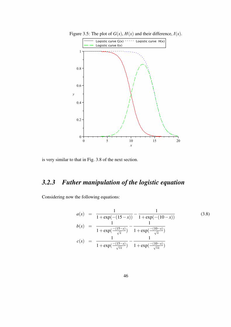
Figure 3.5: The plot of G(x), H(x) and their difference, I(x).

is very similar to that in Fig. 3.8 of the next section.

3.2.3 Futher manipulation of the logistic equation

Considering now the following equations:

a(x) =1

1+ exp(−(15− x))− 1

1+ exp(−(10− x))(3.8)

b(x) =1

1+ exp(−(15−x)√x )

− 1

1+ exp(−(10−x)√x )

c(x) =1

1+ exp(−(15−x)√vx )

− 1

1+ exp(−(10−x)√vx )

46

Figure 3.6: A logistic curve to model insects moving into their last life stage.

Here a(x) is the logistic equation we have seen thus far. In the formulas for b(x) and c(x),

some extra manipulations are made in order to get a form of the logistic equation that

appears in Eq. (1.8) of Chapter 1. In b(x) we introduce a division in the exponential by

a factor of√

x. Furthermore, in c(x) we introduce a division in the exponential of√

vx.

Now we have in c(x) the fully constructed logistic equation for the intermediate stages of

the logistic model of Eq. (1.8). A plot of the three variants of the logistic equations reveals

that as the denominator in the exponential increases, the peak of the intermediate values

decreases, and the spread over which insects can occupy a certain life stage also increases.

Treatment of the effect of changes in the denominator for the beginning and final life stages

of the model are considered in the next section.

It is clear that b(x) is just a special case of c(x) with v = 1. Thus, for comparison

purposes we need only compare a(x) with c(x). First, we should note that a(x) > 0,∀x,

47

while c(x) > 0,x > 0 since c(x) is undefined when x ≤ 0. Another crucial quality of c(x)

is c(x)→ 0 as x → 0+, whereas a(x)→ 0 as x →−∞. This means that c(x) will reach a

value in finite time, and a(x) would require infinite time to reach a minimum of zero. This

is imporatant biologically because we cannot use infinite time in that regard. This point

also lends more credibility to the model with c(x), since it is more realistic than a(x) in a

biological sense.

48

Figure 3.7: A plot of a(x), b(x) and c(x) of equations (3.8).

3.3 Traits of the logistic phenology model

A further examination of the traits of the logistic phenology model in Eq. (1.8) of Ch. 1

may be of interest to certain audiences. For example, one may be interested in how the

parameters affect the shape or the location of the distribution on a graph. Also, one may be

interested in what constraints the model has.

Some of the constraints of the parameters are illustrated here. The values of the ai’s

ought to be consecutive. Otherwise, if we had a case where a4 < a3, then completion of the

third instar would occur after completion of the fourth instar. This does not make biological

sense, and therefore each successive ai should be greater than ai−1. More precisely, we

ought to have the constraint 0 < a1 < a2 < a3 < a4 < a5. Note that we have the constraint

49

that 0 < a1.

The other parameter v has to be greater than zero. Within Eq. (1.8) we see that v is

housed in a square root, and we must have the constraint that v > 0 to obtain biologically

meaningful results. Once all of these traits are satisfied, we get a population distribution

that appears in Fig. 3.8.

Figure 3.8: The logistic phenology model, exhibiting the different instar proportions. Notethat p1(t) contains the proportion of grasshoppers in instar one and below (Dennis andKemp (1988, [10])).

50

The way that this logistic probability function is defined, we get the condition that

6

∑i=1

pi(t) = 1, ∀t. (3.9)

We get a result of unity when we sum all of the proportions because the sum of the propor-

tions is a telescoping sum.

When analyzing the parameter v, it was found that this parameter controls the variance

of the proportions of the grasshoppers in different instars. When analyzing the effect of v

on the distributions, three different values of v were taken. In Figs. 3.9, 3.10, and 3.11, we

have v = 0.4 corresponding to the green graph, which is the dashed-dotted graph. The red

graph, which is the dotted graph, pertains to the situation where v = 4.0; and finally, the

blue-solid graph pertains to the case where v = 40. In Fig. 3.9 we have the first portion of

the logistic probability distribution plotted, or p1(t). When the value of v is low, as in the

green dashed-dotted line, we get a function that rapidly drops off from a proportion of one

to a proportion that approaches zero. For the highest value of v the rate that the function

drops from a proportion of one to a proportion of zero has a much greater spread than that

of the function with lower values of v. Notice that all the graphs in Fig. 3.9 cross at the

same point, at t = a1, which is the point at which the population of grasshoppers in instar

one is fifty percent [9] .

In the intermediate stages of the phenology, we can see that we get a greater variance

over which the model extends as v increases. Also note that the function has a higher peak

when the value of v is decreased. When considering p6(t), we get the situation that occurs

in Figure 3.10. This situation is analogous to that of p1(t) except the function with a lower

value for v will increase from a proportion of zero to a proportion of one very quickly. Also

note here that all three curves intersect at the same point, which is a5, the point where the

grasshopper population is at fifty percent adulthood.

51

Figure 3.9: Plots of p1(t) when v is varied.

52

Figure 3.10: Plots of the intermediate stage p2(t), as v changes.

53

Figure 3.11: Plots of p5(t) as v varies.

When analyzing how the ais affect the phenology model it is easy to see that when

the ais have higher values, the logistic probability curves will be shifted to the right. As

an example, Fig. 3.12 illustrates how increasing the ais will shift the curves further and

further to the right. In the graph of the dotted red line, a2 = 200 and a1 = 100; a2 = 300

and a1 = 200 in the solid blue curve; and a2 = 400 and a1 = 300 for the green dashed

dotted curve. All other things being equal, when we increase the value of the ais we get

curves that are further to the right on a graph of proportion versus degree-days. Also notice

that as the curves are shifted further to the right, the peaks of the curves decline.

Another thing to note is the effect of the spread of the different ais. By inspection,

Fig. 3.13, all of the curves have an a2 = 300, whereas in the red dotted, blue solid, and

the green dashed-dotted curves the a1s are 100, 200, and 275, respectively. In these cases,

the red dotted curve has the highest peak, but this peak occurs at the lowest value in terms

54

Figure 3.12: Holding v constant and increasing the a1 and a2 values for the intermediateprobability p2(t).

of degree-days. The trend in Fig. 3.13 is that as the distance between a2 and a1 is de-

creased, with a2 being held constant, the curves have a smaller peak for the proportion

of the grasshopper population, and those peaks occur at a higher degree-day value. Also,

when observing these graphs, it appears that the peak of these curves occurs approximately

around the average of a2 and a1.

It is worth mentioning whether or not it is always the case that pi(t)≥ 0,∀t. It is clearly

the case for p1(t) = [1 + exp(−(a1−t)√

vt

)]−1. We know that the numerator is always 1, and

the denominator will always be 1 or greater since the exponential will always be positive,

and will only vanish as t →+∞. Therefore, the denominator 1 + exp(−(a1−t)√

vt

)≥ 1, ∀t,

giving the required condition p1(t)≥ 0, ∀t.

For the intermediate stages, we know that [1 + exp(−(ai−t)√

vt

)]−1 ≥ 0 ∀i, t and we also

55

Figure 3.13: A plot illustrating what happens when v and a1 are held constant and a2 isallowed to vary.

know that ai > ai−1. Thus, all we need to verify is whether the first term is greater than the

term being subtracted. Using inequalities, we get:

ai > ai−1 (3.10)

−(ai− t) < −(ai−1− t)

exp(−(ai− t)√

vt) < exp(

(ai−1− t)√vt

)

1

1+ exp(−(ai−t)√vt )

>1

1+ exp( (ai−1−t)√vt )

In the last line of the inequalities of (3.10) we get the desired result, which implies that

pi(t)≥ 0,∀t in the intermediate cases of the logistic model.

For the final stage of the model we know that the term being subtracted, [1+exp(−(a5−t)√

vt

)]−1

56

is always greater than or equal to zero. Also, it is apparent that exp(−(a5−t)√

vt

)> 0, which

implies that [1+exp(−(a5−t)√

vt

)]−1 < 1. Therefore, subtracting this term from 1 will give us

the desired result, pi(t)≥ 0,∀t. Thus the inequality pi(t)≥ 0,∀t holds for all stages of the

logistic model.

57

Chapter 4

Fitting the model

4.1 Chapter overview

In this chapter, a general description of nonlinear regression is given, as is a description of

the optimization algorithm that my logistic phenology model uses. This chapter analyzes

and highlights some of the problems with choosing initial values for parameter estimation

within my model. Also, possible solutions to the problem of choosing initial values and

solving for the model’s parameters are explained.

4.2 Introduction to nonlinear regression

Regression is a mechanism for fitting data to any selected equation. As is the case with a

simple linear regression, the goal of nonlinear regression is to find values for parameters

that minimize the sum of the squares of the distances of the data points to the curve (Mo-

tulsky and Ransas (1987, [49])). If the value for each observation is yi, and the predicted

value for the function is yi, the goal is to minimize the sum of squared errors (SSE), with i

observations:

SSE =n

∑i=1

(yi − yi)2. (4.1)

This method of optimization is known as the least squares method, because the sum of

squares of the distances between the observations and predictions is being minimized.

58

4.2.1 Initial regression attempts

Consider the first part of Eq. (1.8) of Chapter 1:

p1(t) = (1+ exp(−(a1− t)√

vt))−1 (4.2)

Regression can be used to determine the values for v and a1. First, it would be prudent

to perform some transformations in order to make the regression more manageable. The

transforms are as follows:

q1(t) =1

p1(t)= 1+ exp

(−(a1− t)√vt

)

r1(t) = q1(t)−1 = exp(−(a1− t)√

vt

)

s1(t) = ln(r1(t)) =t−a1√

vt(4.3)

Now if we let u =√

t and β = 1√vt we get the following formula:

α1(u) = βu− βa1

u(4.4)

Where αi = predicted value (function value) and αi = the observed value with u = u1,u2, ...,un

and α = α1,α2, ....,αn. In this case our SSE1 becomes:

SSE1 =n

∑i=1

(αi− αi)2 (4.5)

59

By expanding the SSE1 term we get:

SSE1 =n

∑i=1

(αi− αi)2=

(n

∑i=1

α2i −2β

n

∑i=1

αiui+

2a1βn

∑i=1

αi/ui +β2n

∑i=1

u2i +a2

1β2n

∑i=1

1/u2i −2β2a1n

) (4.6)

Now taking partial derivatives of the SSE with respect to a1 and β, and setting the partial

derivatives to zero, we obtain the so-called normal equations:

∂SSE1

∂a1= −nβ2 +a1β

n

∑i=1

1u2

i+

n

∑i=1

αi

ui= 0 (4.7)

∂SSE1

∂β= −

n

∑i=1

αiui +a1

n

∑i=1

αi

ui+β

n

∑i=1

u2i −2na1β+βa2

1

n

∑i=1

1u2

i= 0

When the above pair of equations with two unknowns are solved, we obtain the following

for solutions for β and a1:

a1 =nβ−∑n

i=1αiui

β∑ni=1

1u2

i

β =∑n

i=1 αiui ∑ni=1

1u2

i−n∑n

i=1αiui

∑ni=1

1u2

i∑n

i=1 u2i +n2

(4.8)

Let us continue to use regression to solve for the parameters in the full SSE. We know

a1 and v from our first regression. Now a second SSE (SSE2) can be set up.

SSE2 =j

∑i=1

(p2i(ti)− (1+ exp(

−(a2− ti)√vti

))−1 (4.9)

+(1+ exp(−(a1− ti)√

vti))−1

)2

Here, p2i(ti) is the observed values of the proportion of the population in the second instar

60

at time ti.

At first glance, SSE2 seems like it may be a good candidate for a regression in order to

solve for a2. Since we know the values of a1 and v from the first regression, SSE2 is just

a function of a2. If we let x =(

1+ exp(−(a2−ti)√bti

))−1

and y =(

1+ exp(−(a1−ti)√bti

))−1

, and

take the partial derivative of SSE2 with respect to a2, we get

∂SSE2

∂a2=

j

∑i=1

2(p2i(ti)− x+ y)x−1

y2√

bti= 0. (4.10)

This is obviously a cumbersome equation to solve, so looking at a numerical method for

solving a2 and successive ai values seems like a logical option.

4.3 Numerical methods

Most fitting of nonlinear equations to data cannot be solved in one step, unlike the fitting of

linear or polynomial equations to data. Fitting nonlinear equations to data must typically

be done iteratively. To begin the iterative process, the user of a nonlinear fitting algorithm

must supply initial values or guesses for the parameters in the particular equation that is

being fitted. The nonlinear regression procedure then adjusts these initial values to improve

the fit of the function to the data. The parameters continue to be adjusted to keep improving

the fit of the equation to the data. Iterations will continue in the algorithm until negligible

improvement of the fit occurs. A tolerance or threshold for improvement is established at

the outset of the curve fitting procedure. Once the amount of improvement in the fit of the

data falls below the tolerance, the iterations of the procedure are halted, and values for the

parameters at last iteration are selected.

61

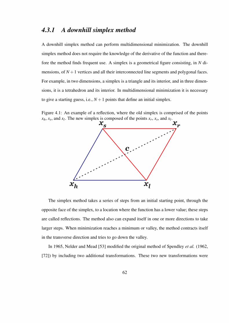
4.3.1 A downhill simplex method

A downhill simplex method can perform multidimensional minimization. The downhill

simplex method does not require the knowledge of the derivative of the function and there-

fore the method finds frequent use. A simplex is a geometrical figure consisting, in N di-

mensions, of N +1 vertices and all their interconnected line segments and polygonal faces.

For example, in two dimensions, a simplex is a triangle and its interior, and in three dimen-

sions, it is a tetrahedron and its interior. In multidimensional minimization it is necessary

to give a starting guess, i.e., N +1 points that define an initial simplex.

Figure 4.1: An example of a reflection, where the old simplex is comprised of the pointsxh, xs, and xl . The new simplex is composed of the points xr, xs, and xl .

The simplex method takes a series of steps from an initial starting point, through the

opposite face of the simplex, to a location where the function has a lower value; these steps

are called reflections. The method also can expand itself in one or more directions to take

larger steps. When minimization reaches a minimum or valley, the method contracts itself

in the transverse direction and tries to go down the valley.

In 1965, Nelder and Mead [53] modified the original method of Spendley et al. (1962,

[72]) by including two additional transformations. These two new transformations were

62

Figure 4.2: An example of an expansion of the simplex. The old simplex is as in Fig. 4.1and the new simplex is xh, xs, and xc.

Figure 4.3: An outside contraction of the simplex. The old simplex is as in Fig. 4.1 and thenew simplex is xh, xs, and xc.

expansion and contraction, that allow the working simplex to change not only its size, but

also its shape. By doing so the simplex could adapt itself to the local landscape, elongating

down long inclined planes, changing direction on encountering a valley at an angle, and

contracting in the neighbourhood of a minimum.

To better illustrate the movements of the simplex, consider a simplex in two dimen-

sional space. In this case, the algorithm first orders the vertices based on the value they

produce for the function being minimized. For our example the indices h, s and l refer to

63

Figure 4.4: An inside contraction of the simplex. The new simplex and old simplex are thesame as those in the last figure.

the worst vertex, second worst vertex, and best vertex respectively. The term worst here

means that the vertex produces the largest value for the function being minimized, for all

the vertices. The vertices associated with these indices are xh, xs, and xl . These vertices in

turn produce function values fh, fs, and fl , which correspond to the highest function value,

the second function value, and the lowest function value, respectively.

The algorithm now calculates the centroid, c, of the best side. The best side is the one

opposite the worst vertex xh. After the centroid is calculated, the simplex goes through a

series of transformations. First a reflection point xr is calculated and its associated function

value fr. The vertex xr is accepted if fl ≤ fr < fs, and the iteration is terminated. The

reflection can be seen in Fig. 4.1.

If fr < fl an expansion vertex, xe, is computed along with the function value, fe, asso-

ciated with that vertex. If fe < fl then the vertex xe is accepted and the iteration is halted.

If fe ≥ fr then xr is accepted and the iteration is terminated. The expansion transformation

is illustrated in Fig. 4.2.

When the reflections do not work, the simplex will either perform contractions or it will

shrink. If fr ≥ fs then a contraction point, xc, is calculated. The contraction can be either

64

Figure 4.5: Shrinking of the simplex. The old simplex is the larger of the two triangles.

an inside contraction or an outside contraction. If fs ≤ fr < fh, an outside contraction is

computed; and if fc ≤ fr is accepted then the iteration is terminated. An inside contraction

is computed if fr ≥ fh, then if fc < fh the inside contraction is accepted and the iteration is

terminated. The outside contraction is in Fig. 4.3 and the inside contraction is in Fig 4.4. If

either of the contraction points is not accepted then a shrinking of the simplex occurs. The

shrink transformation is seen in Fig. 4.5.

Like all minimization algorithms, the convergence criteria can be complicated. Further-

more, since there is more than one variable, it is possible to define different tolerances for

each variable, but that was not the method employed in our simplex algorithm. Our method

of checking for convergence is to determine when the maximum distance between vertices

is lower than some predetermined value (Nelder and Mead (1965, [52]), Olsson and Nelson

(1975, [57]), Price et al. (2002. [59]), Singer and Singer (2004, [70]), [47] ).

65

4.3.2 Problems associated with nonlinear regression

There can be many problems associated with a simplex method when choosing the initial

values of the starting simplex, just as there can be some problems associated with choosing

initial values for parameters in other numerical recipes for nonlinear optimization. Poor

selection of initial values may have some of the following consequences:

1. In a well-behaved system, the amount of computer time required to reach a solution

will be increased.

2. Poor choice of initial values may lead the nonlinear regression program to go off in

the wrong direction and never converge to a solution.

3. It is also possible that selection of certain initial values can cause the nonlinear pro-

gram to get trapped in a local minimum which provides incorrect values for parame-

ters.

4.4 Constructing the simplex

When constructing the simplex, values must be chosen for the different vertices of the sim-

plex. Our optimization problem contains six parameters that must be solved for; therefore,

we need seven unique vertices for our simplex in order for the algorithm to work correctly.

When choosing initial values for the simplex one must be careful to follow the con-

straints that each successive ai is larger than the prior one. We must also have the constraint

that all of our parameters are greater than zero.

Implementing initial values of the parameters that do not abide by the constraints 0 <

a1 < a2 < a3 < a4 < a5 and v > 0 can lead to a variety of situations.

When investigating ways to come up with initial values for the vertices of the starting

66

simplex, a few methods were examined. In one method we tried to do successive regres-

sions on the pi(t)s. In a sense, we tried to bootstrap our way up through the expressions

for the different proportions for the instars and along the way pick off values for v and

the subsequent ais. Starting off with p1(t), equations for a1 and v presented themselves.

Utilizing the observed instar counts and degree-days accumulated on a certain date for a

certain region, we were able to solve for the parameters a1 and v.

Although the methods for solving a1 and v are sound, some other problems presented

themselves when solving for other parameters. One of the less-than-ideal results that this

type of bootstrapping led to was a violation of the constraint ai−1 < ai, which is not biolog-

ically feasible. Trying to fix the violation of the constraint involved decisions on what data

was useful and what data should be discarded. These decisions made the method impracti-

cal and convoluted, even for an experienced user; therefore, a more pragmatic approach to

the initial value problem for the simplex was needed.

When looking for ways to find a range of the degree-days over which our model is

forecasting grasshopper development, one could use the method of moments like approach.

For example, we know that parameters a1 and a5 correspond to the times when half the

grasshopper population is occupied by first instar grasshoppers and adult grasshoppers,

respectively. Thus one could find the average of the observed proportions of grasshoppers

in these stages, which would be precisely the parameters a1 and a5. This method also has

some shortcomings with regards to its applicability to timing pest control solutions. One of

the disadvantages of this method is that we cannot estimate the parameters for intermediate

stages (a2, a3, and a4), nor can we estimate the parameter v. For practical use, there is

to be no value added to this model in forecasting a5 in this manner, since it will occur

after the pests are well into adulthood, and the vast majority of damage to crops is done.

However, this method can be useful when analyzing historical data in that it would help

put a range on starting dates and ending dates during which the majority of pest activity is

67

taking place, both in Julian and degree-days. Also, the method of moments coupled with

historical data could give better indications as to how future grasshopper forecasts might

unfold with respect to results typified by certain climatic conditions. Still a simpler method

of approximating parameters was needed.

A heuristic method that was tried was an evaluation of a range of degree-days for which

some of the instars’ populations were peaking in terms of the observations for that day. For

example, if we know all of the proportions for our observations, and all of the degree-day

accumulations of all the days on which the observations were taken, we could hypothesize

about when instar peaks are occurring, or when phenological stages are completing. The

advantage of this method is that it allows us to keep the constraints of our parameters intact,

since we know the biological meanings of our parameters. We know that ai is the amount

of time required for a grasshopper to complete the ith phenological stage for intermediate

instars where 1 < i < 5. Also, we know that a1 and a5 indicate where fifty percent of the

grasshopper population is in that instar. Knowing when the molting from one phenological

stage to another, or when the instars may be peaking, would then give us a range over

which to choose the subsequent ais for the initial values of the simplex. Even knowing how

much heat is required for a grasshopper to graduate from one instar to the next would also

allow us to hypothesize a range for the ais. Based on how fast heat is accumulating for

a particular year in which the data is gathered, we could estimate how fast a grasshopper

would move through a life stage, which would in turn give us an idea of how the variability

of each life stage may look, modelled by the parameter v.

4.5 Analyzing related miniature models

When performing any type of nonlinear regression there is always a chance that the al-

gorithm can converge to a wrong (wrong in terms of the parameters not abiding by their

68

constraints) local minimum. Knowing that this is a distinct possibility, it may be worth

investigating an SSE in order to answer such questions as: Is there one global minimum,

and if so, does it abide by the constraints? How many local minima could there possibly

be? How should we construct our simplex so we get into a local minimum that gives a

feasible or workable solution?

Since we cannot visualize beyond 3-dimensional space, the best way to analyze our

6-dimensional SSE is to look at smaller versions of the optimization problem. This would

entail reducing the number of parameters in our model to deal only with a1 and v, or a1,

a2 and v. The latter case would be ideal since salient features such as the constraints for

successive instars would be retained.

4.5.1 A miniature optimization problem

Before starting the analysis of the full SSE, it is prudent to start first with a very simplistic

view of a smaller optimization problem. The first case one could conceivably look at is the

case where there are only two parameters, a1 and v. Biologically, most insects, with a few

exceptions, develop from an egg and then have stages where molting occurs [86, 78]. Even

though this is a purely biological concern, it can be put aside in the interest of looking at the

mathematics, mechanics and features of putting together a model that is a simpler version

of our 6-dimensional model. This most miniature version of the full model may enlighten

us as to how the larger model is behaving.

Fig. 4.6, is an illustration of what the SSE looks like for the mini-model. The particular

SSE for this illustration contains three contrived data points. In Fig. 4.6 we get an idea

of how the SSE is shaped. The unlabeled axis is the value of the SSE. In this simplistic

model we can see that the SSE is smooth and only appears to have one local minimum.

69

The particular contrived SSE that gives Fig. 4.6 is

SSE(a1,v) =((

1+ exp(−(a1−50)√50v

))−1

−0.85)2

+((

1−1+ exp(−(a1−50)√50v

))−1

−0.15)2

+((

1+ exp(−(a1−100)√100v

))−1

−0.7)2

+(

1−(

1+ exp(−(a1−100)√100v

))−1

−0.3)2

+((

1+ exp(−(a1−200)√200v

))−1

−0.2)2

+(

1−(

1+ exp(−(a1−200)√200v

))−1

−0.8)2

. (4.11)

The degree-days contrived here are 50, 100 and 200 degree-days respectively. The corre-

sponding p1s for those respective degree-days are 0.85, 0.7 and 0.2. Also the corresponding

p2s are 0.15, 0.3 and 0.8. Also note that in this model the insect being modelled can only

be in one life stage, hence the population is always in the first instar. Not much insight can

be gathered from this mini-model; thus, considering a model with more parameters would

be the next option. With larger optimization models, as the value of v gets smaller, there

are more local minima where a simplex might get trapped.

4.5.2 Another miniature optimization

The next logical step is to look at a model with parameters a1, a2 and v. Also, in this

model the constraints a2 > a1 and v > 0 can both be imposed. With this model, we can

contrive data, create different situations, and study the SSE for local minima. Also, by

holding one parameter constant, we can look at other parameters and 3-dimensional plots

of parameters that are allowed to vary, and see what happens to the shape of the SSE. Even

with the 3-dimensional plot, we can only surmise how the surface of the SSE may look

in four dimensions. Since we cannot view 4-dimensional space, there may be occurrences

when the simplex gets trapped in local minimum with an improper solution, with respect

70

Figure 4.6: A look at the SSE from a vantage point outward from the origin and the v-axis.The unlabeled axis is the value for the SSE.

to the parameters and their constraints. However, this analysis may provide information

regarding a suitable region to construct the simplex in.

When investigating the SSE below, a1 and a2 were allowed to vary while keeping v

constant at 20 initially. This yielded illustrations where the surface of the SSE is very

smooth. However, when we change the value of v to v = 1, situations arise where there are

many minima as in Figs. 4.7 and 4.8. In these figures we can see that there are many more

peaks and valleys. In this instance, a simplex could easily get trapped in different minima,

depending on where the simplex starts, and could subsequently give extraneous solutions

71

for the parameters. The SSE in Eq. 4.12 is a function of a1 and a2 with v = 1 and is

SSE(a1,a2) =((

1+ exp(−(a1−50)√50

))−1

−0.85)2

+(

1−(

1+ exp(−(a2−50)√50

))−1

−0.04)2

+((

1+ exp(−(a2−50)√50

))−1

−(

1+ exp(−(a1−50)√50

))−1

−0.11)2

(4.12)

+((

1+ exp(−(a1−100)√100

))−1

−0.7)2

+((

1+ exp(−(a2−100)√100

))−1

−(

1+ exp(−(a1−100)√100

))−1

−0.2)2

+(

1−(

1+ exp(−(a2−100)√100

))−1

−0.1)2

+((

1+ exp(−(a1−200)√200

))−1

−0.1)2

+((

1+ exp(−(a2−200)√200

))−1

−(

1+ exp(−(a1−200)√200

))−1

−0.5)2

+(

1−(

1+ exp(−(a2−200)√200

))−1

−0.4)2

Inspection of the SSE shows that the three data points have degree-day values of 50, 100,

ad 200 respectively. The corresponding p1s for these degree days are 0.85, 0.7, and 0.1

respectively. The p2s are 0.11, 0.2 and 0.5 while the p3s are 0.04, 0.1 and 0.4.

Noting that valleys become more prevalent as the value of v gets very small, one les-

son we could take away from looking at the miniature model is to have initial guesses for

the parameter v starting away from relatively low values such as v ≤ 1. Some researcher

(Onsanger and Kemp (1986, [54]), and Dennis et al. (1986, [9])) have found v with lower

bounds of at least 4 for some species of grasshoppers, which lends some plausibility to con-

structing a simplex away from lower values of v. In the next chapter, there will be a further

discussion of parameters that we obtained compared to parameters that other researchers

72

have obtained.

Another variable that affects the complexity of the SSE is the number of data points

sampled. The SSE surface will generally get more complex as more data points are taken

into consideration. For example, we can compare and contrast Fig. 4.7 and Fig. 4.8. In

Fig. 4.7 we have the SSE with three data points that was already listed for this miniature

model. In Fig. 4.8 note that there are a total of six data points. The surface of the SSE

in Fig. (4.10) is more complex in the sense that the surface seems crumpled and has more

distinct valleys in which a simplex might be caught.

Figure 4.7: The surface of an SSE with only three data points, from our mini-model withparameters a1, and a2 varying with v=1.

73

Figure 4.8: The surface of an SSE with six data points, again allowing a1 and a2 to varywhile keeping v=1. The surface seems generally more complex than in Fig. 4.7. The a1axis is the left axis in this illustration whereas the a2 axis is the right axis. The vertical axisis the value of the SSE.

4.6 SSE for the full model

In the full model, there is a total of six parameters. The parameters a1 through a5 are

measures of phenological growth of the grasshoppers, and v is related to the duration that

a grasshopper can occupy a certain phenological stage in terms of degree-days. Again,

we cannot visualize what the surface of the SSE would look like in 6-dimensional space;

however, the SSE can be viewed while holding four parameters constant and allowing the

other two parameters to vary.

When looking at the SSE, there was interest to see how it would react if v was varied.

By inspecting the 3-dimensional figures for the SSE, it became clear that as v decreased in

value, there was an increase in the number of local minima that were occurring.

74

Figure 4.9: Here v = 1 and we can see that there are peaks and valleys occurring.

In Figs. 4.9 and 4.10, we are allowing a3 and a4 to vary while having v = 1 and v = 0.5,

respectively. These two cases have more than one local minimum as compared to the case

where v = 20. Also as v decreases from 1 to 0.5, the minima are more pronounced; that is,

the valley floors contain steeper walls. This conclusion is apparent in comparing Figs. 4.9

and 4.10. Also note that in this full model, the SSE is comprised of six data points, but the

equation for the particular SSE is not listed because it is very large.

The same conclusion can be made from analysing both the miniature model and the full

model. When constructing a simplex, the values corresponding to the parameter v ought

to be away from lower values. Having v start further away from lower values in turn helps

the simplex to avoid the region where the SSE surface has many local minima. In our case

we should not begin with simplex values of v close to 1, but further out, such as v = 5 or

greater in order to maintain an SSE that has a surface with possibly fewer local minima.

75

Figure 4.10: In this figure v = 0.5, and we are looking at the surface of SSE. The unlabeledaxis is the value of the SSE. The peaks and valleys seem more pronounced here than in Fig.4.9.

76

Chapter 5

Results and conclusions

5.1 Chapter overview

The final model uses the improved degree-day accumulators developed in Chapter 2, and

analysis of Eqn. (1.8) that was done in Chapter 3. Also, while developing and testing the

final model, Chapter 4 was necessary in order to inform readers of the process and some

of the problems encountered when using the final model. Chapter 5 explains some of the

data that was used when running our logistic phenology model, and some prior work done

using this model. Also this chapter gives some suggestions that researchers may want to

take into account when using this model in the future.

5.2 Running the logistic phenology model with real data

One species of grasshopper with available data was Melanoplus sanguinipes. This species

was observed in the vicinity of the town of Onefour, located in southwestern Alberta. The

observations were made between June and September 2000, for six particular dates. When

running our simplex method for finding the six different parameters, we used a development

threshold of 12 ◦C. The results obtained for each of the different degree-day accumulators

are listed below in Table 5.1.

Table 5.1: Parameters estimates for M. sanguinipes at Onefour for the year 2000.Degree-day method a1 a2 a3 a4 a5 v

Linear heating and cooling 105.33 197.95 355.71 473.92 549.94 27.83Traditional sine 110.12 203.69 358.75 491.67 575.38 27.56

Sine heating and linear cooling 108.65 200.71 357.32 481.53 565.49 28.78Sine heating and cooling 111.21 203.02 357.43 495.28 578.46 26.93

77

The values of the ai parameters are fairly consistent throughout the analysis, with the

biggest gap of ≈ 28 degree-days between the a5 values when comparing the linear heating

and cooling accumulator and the sinusoidal heating and cooling accumulator. The differ-

ence in the highest and lowest values for the parameter v was 1.85.

5.3 Comparisons to other studies

The species M. sanguinipes was also studied by Onsanger and Kemp (1986, [54]) using the

same model. The collection of their grasshopper data was done in approximately weekly

intervals during the summer months of 1975 and 1976 near Roundup, Montana. In the

year 1975, grasshoppers were collected for 22 weeks, and in 1976, grasshoppers were col-

lected for 19 weeks. Thus, Onsanger and Kemp have 22 and 19 observations respectively,

compared with our six observations for the year 2000 at Onefour, Alberta. Also, there

is a geographical difference in that Roundup, Montana, is located approximately 415 km

southwest of Onefour, Alberta.

Table 5.2: Grasshopper counts (M. sanguinipes) at Onefour for the year 2000, for six dif-ferent dates.

Date Instar 1 Instar 2 Instar 3 Instar 5 Instar 5 Adult TotalJune 22nd 34 59 118 17 1 0 229

July 6th 20 26 39 22 9 1 117July 18th 8 59 74 27 31 24 223

August 1st 0 9 32 24 17 35 117August 15th 0 0 3 17 23 89 132

September 9th 0 0 0 0 1 39 40

There were several other differences in methodology of collecting data that can account

for differences in the parameters obtained from our model and that of Onsanger and Kemp.

One of these was that Onsanger and Kemp recorded air temperature at 5cm above ground,

whereas our temperature was obtained 2m above ground. Also, Onsanger and Kemp used

78

only the traditional sine wave method for calculating degree-day accumulations, with a

developmental threshold of 17.8 ◦C. Our model contains four methods for calculating the

degree-day accumulation, with a threshold of 12 ◦C. Another difference is that they started

their accumulation of degree-days on May 6th of each year. Our model can take into ac-

count degree-day accumulation for the whole year, but typically degree-day accumulations

begin on April 1st of the year. Also, the traditional sine wave method for degree-day ac-

cumulation does not take into account the geographic location of the grasshopper observa-

tions, nor the daily temporal aspect of heating and cooling that occurs during the day. Dif-

ferences in biofix dates and temperature thresholds come from difference in preferences,

location, and laboratory results that different researchers use (Hewitt (1979, [20]), Kemp

(1987, 1989, [32], [34]), Kemp and Dennis (1991, [35]).

The parameters for Onsanger and Kemp’s work are in Table 5.2. As shown, the ai val-

Table 5.3: Parameter estimates for M. sanguinipes for the years 1975 and 1976 nearRoundup, Montana.

Year a1 a2 a3 a4 a5 v1975 54.66 111.85 148.45 199.89 287.99 5.191976 80.76 124.96 168.86 283.54 391.61 9.99

ues obtained by Onsanger and Kemp are much lower than our ai values. This is likely due

to Onsanger and Kemp using such a high threshold of 17.8◦C. By using a lower thresh-

old like 12 ◦C, Onsanger and Kemp would have gotten higher ais (since more degree-day

accumulation would occur), and consequently it would imply that the grasshoppers were

spending more time (in terms of degree-days) in a certain phenological stage. This would,

in effect, increase the spread of the logistic curves, and subsequently, Onsanger and Kemp

would have obtained a higher v value, with a lower developmental threshold.

One comparison is to take a developmental threshold of 17.8◦C and run the model

using our degree-day accumulators. To do this, the initial values for our simplex must

79

be augmented to take into account a higher threshold resulting in lower accumulations

occurring when compared to a threshold of 12 ◦C. Here again we are using the same data

for Onefour from the year 2000. We obtain the following:

Table 5.4: Parameter estimates for M. sanguinipes at Onefour for the year 2000, using athreshold of 17.8 ◦C.

Degree-day method a1 a2 a3 a4 a5 vLinear heating and cooling 1.29 76.79 138.87 159.84 161.32 2.03

Traditional sine 5.28 91.29 137.39 213.97 246.77 1.59Sine heating and linear cooling 13.26 67.24 132.45 188.92 193.15 1.57

Sine heating and cooling 13.41 99.30 151.73 187.91 225.33 1.70

Comparing this table with Table 5.2, we can see that the v values are lower than those

achieved by Onsanger and Kemp. Here we can also see that the parameter a1 has low

values, and it seems implausible to have such small values for the first phenological stage.

However, the comparison for this parameter can be problematic, since we are at a different

geographic location during a different year. Also, the other parameters in table 5.3 have

lower values than Onsager and Kemp’s work.

5.3.1 Problems with comparing data

There are many potential differences in the ways the data was collected between our model

and the Onsanger and Kemp model, our comparison relates only to the basic differences in

the temperature and values of the parameters. Also, the grasshopper counts and temperature

data that Onsanger and Kemp used are not available. Moreover, there is no information

readily available on what they used for initial values for their simplex in the Nelder-Mead

algorithm. Thus, we are not in a position to either refute or confirm their results.

Although authors like Onsanger, Kemp, and Dennis derived this logistic phenological

model, they do not mention some of the difficulties involved with using the Nelder-Mead

80

algorithm that this thesis discusses. For reasons unknown, these authors do not give a

rigorous mathematical treatment of the model. For example, their papers on this model do

not mention the pitfalls of a simplex falling into a local minimum that may give extraneous

parameters. Although the constraints for the parameters might be implied in their papers,

they are never directly expressed.

5.4 Improvements and future work

One possible way to improve upon this model is to reduce the number of parameters in the

model, thus making the SSE less cumbersome. The duration that a typical pest grasshopper

spends in the first instar is very short (Johnson 2008, [29]); thus, we could pool the first

and second instar grasshoppers into one category, thereby combining a1 and a2 into one

category. By doing this, we would reduce the complexity of the SSE and perhaps get a

more accurate range over which the first and second instars may be occurring.

Other intermediate stages could be pooled together, depending on the researcher’s

needs, which may benefit his or her work. For example, a researcher may want to group

the first and second instar together, and the third and fourth instar together, thereby reduc-

ing the minimization problem from six parameters to four parameters. This may add value

to those researchers who are concerned with pest management strategies and schedules, in

that they may lump together instars in which the grasshopper is most voracious, thus giving

a better time frame in which to apply pesticides.

Pooling of instars ought to be used with caution, however. The parameter v is a measure

of dispersion of the instars that remains constant throughout the use of the model. Obvi-

ously, when two or more instars are pooled, it increases the amount of the time that the

grasshoppers will be spending in the hybrid instar, thereby changing v for the whole model.

Thus, one ought to take caution when attempting to pool instars, since such changes will

81

affect the resulting parameters.

Because information is the prime driver for the majority of models and confidence is

created by replication, another way to improve this model would be to gather more data

from different locations during different years and run the model against this new data in

order to make more comparisons. Also, by gathering more historical data and running

the model with said data, we can test what the model is predicting versus what actually

happened in the field. By doing so, the model can be refined in order to become more

robust and precise.

The task of collecting grasshoppers and properly identifying them is a time-consuming

and laborious task, and could be a potential barrier for any kind of model involving the

phenological stages of the grasshopper. Moreover, gathering all the weather data for the

corresponding collection of grasshopper data is also very time-intensive. The cost and

manpower needed to accomplish these things could hinder improvements to the model, in

terms of gathering more data. One way to reduce the manpower needed to do this task

would be to take roadside survey counts (Johnson (1989, [30])).

Another potential hurdle to this model is that a general user may not be familiar with

the constraints necessary when determining the values for the initial simplex. By having

experts put into place hard coded data for different scenarios, the problem of selecting

the initial values for the simplex could be overcome. However, this comes at the price of

gathering more data, more comparisons and more manpower.

Improvements in gathering temperature data could also contribute improvements for

this model. For example, if temperatures are taken not only at 2m but at 5cm above the

ground, researchers would have a better estimate of what is going on in the micro-climate

in which the grasshoppers live.

Other future work that this model could produce is a stochastic phenology model for

other insects that have temperature as their primary driver for growth. The code for this

82

model is very general, and we used data for grasshoppers; however, it can be used to model

other organisms that have temperature-driven growth and activities.

Working with this model first hand, I observed that it has limitations in that it can be

very time intensive to model even one set of data point for one location. This results from

time devoted to choosing initial values for parameters in the simplex, and also requiring

the acquistion of data from the field. Acquistion of field data for a large variety of habitats,

and for a variety of dates would also be time consuming. The conversion of temperature to

degree-days is also time consuming in that the temperature data must be formatted properly

to be used in conjunction with our program.

To overcome these hurdles future researchers could use the Lactin and Johnson model

since it only relies on temperature, and four parameters for each life stage [37]. The beauty

of this model is that once the paramters are determined, whether it be in the laboratory or

field, they do not need to be recalculated. With the logistic phenology model, the param-

eters must be calculated evertime the model is run. Thus, the Lactic and Johnson model

has the potential to expedite the modeling process since it would not require calculating

initial cvalues for a simplex, nor would it require a conversion to degree-days. One lengthy

component of modeling that would remain the same would be the collection of the weather

data from available sources.

83

Appendix A

Widespread use of degree-days

United States:

Alabama:

Hendricks, Harlan J., and M. L. Williams. 1992. Life history of Melanaspis obscura

(Homoptera: Diaspididae) infesting Pine Oak in Alabama. Entomological Society of Amer-

ica. 85(4): 452-457.

Connecticut:

Kingsolver, J. G. 1989. Weather and the population dynamics of insects: integrating

physiological and population ecology. Physiological Zoology. 6(2): 314-334.

http://www.jstor.org/stable/30156173

Hawaii:

Vargas, R. I., W. A. Walsh, E. B. Jang, J. W. Armstrong, and D. T. Kanehisa. 1996.

Survival and development of immature stages of four Hawaiian fruit flies (Diptera: Tephri-

tidae) reared at five constant temperatures. Entomological Society of America. 89(1): 64-

69.

Illinois:

Gu, W. D. and R. J. Novak. 2006. Statistical estimation of degree days of mosquito

development under fluctuating temperatures in the field. Journal of Vector Ecology. 31(1):

107-112.

Changnon, D., M. Sandstrom, and J. Astolfi. 2010. Using climatology to predict the

first major summer corn earworm (Lepidoptera: Noctuidae) catch in north central Illinois.

Meteorological Applications. 17(3): 321-328.

84

Kansas:

Charlet, L. D. 1987. Emergence of the sunflower stem weevil, Cylindrocopturus adsper-

sus (Coleoptera: Curculiondae), relative to calendar date and degree-days in the Northern

Great-Plains. Journal of the Kansas Entomological Society. 60: 426-432.

Kentucky:

University of Kentucky summary of insect degree day models:

http://www.ca.uky.edu/agc/pubs/id/id93/app.pdf

Nebraska: Stilwell, A. R., R. J. Wright, T. E. Hunt. 2010. Degree-day requirements

for alfalfa weevil (Coleoptera: Curculionidae) development in eastern Nebraska. Environ-

mental Entomology. 39(1): 202-209.

New Hampshire:

Use of growing degree-days for insect management:

http://extension.unh.edu/agric/GDDays/Docs/growch

Ohio:

Insect degree-day websites used in Ohio:

http://www.entomology.umn.edu/cues/Web/049DegreeDays.pdf

http://www.ipm.msu.edu/landscapeipm/gddarticle.htm

http://extension.entm.purdue.edu/publications/B504.pdf

Oregon:

Insect degree-day websites used in Oregon:

http://climate.usurf.usu.edu/includes/pestFactSheets/degree-days08.pdf

http://www.fs.fed.us/pnw/pubs/pnwrn482.pdf

Pennsylvania:

Georgian, T. and B. Wallace. 1983. Seasonal production dynamics in a guild of

periphyton-grazing insects in a southern Appalachian stream. Ecology. 64: 1236-1248.

85

Utah:

Using degree days to time treatments for insect pests. Utah State University website:

http://climate.usurf.usu.edu/includes/pestFactSheets/degree-days08.pdf

Washington:

Olsen, K. N., W. W. Cone, and L. C. Wright. 1998. Influence of temperature on grape

leafhoppers in south central Washington. Environmental Entomology. 27: 401-405.

West Virginia:

Rock, G. C., R. E. Stinner, J. E. Bacheler. 1993. Predicting geographical and within-

season variation in male flights of 4 fruit pests. Environmental Entomology. 22: 716-725.

Wisconsin: Insect degree-day website used in Wisconsin:

http://www.entomology.wisc.edu/cullenlab/insects/degreedays.html

Wyoming:

Brewer, M. J., and K. M. Hoff. 2002. Degree-day accumulation to time initiation of

sampling for alfalfa weevil using on-site, near-site, and regional temperature data. Journal

of Agricultural and Urban Entomology. 19: 141-149.

86

Canada:

Ontario:

Laing, J. E. and J. M. Heraty. 1984. The use of degree-days to predict emergence

of the apple maggot, Rhagoletis pomonella (Diptera: Tephritidae), in Ontario. Canadian

Entomologist. 116: 1123-1129.

Laing, J. E. and J. A. K. Reid. 1976. Developmental threshold and degree-days to

adult emergence for overwintering pupae of apple maggot Rhagoletis pomonella (Walsh)

collected in Ontario.Proceedings of the Entomological Society of Ontario. 107: 19-22.

Quebec:

Boivin, G. and D. L. Benoit. 1987. Predicting onion maggot (Diptera: Anthomyiidae)

flights in southwestern Quebec using degree-days and common weeds. Phytoprotection.

68: 65-70.

Alberta, Saskatchewan, Manitoba:

Insect Pest Monitoring Network (IPMN)

http://www.westernforum.org/IPMNMain.html

International cases:

Brazil:

Neves, A.D., M. D. Haddad, N. G. Zerio. 2010. Temperature requirements and genera-

tion number estimates of croton mealybug reared in Rangpur lime. Pesquisa Agropecuaria

Brasileira. 45: 791-796.

87

Appendix B

A comparison of degree-day accumulation methods for var-

ious years on the Canadian Prairies.

The following is a list of cities across the Canadian Prairies, and a comparison of three dif-

ferent types of degree-day accumulators and the total degree-day accumulation that occured

for each year. The three accumulators are the temporal sine method which was constructed

for the logistic phenology model outlined for this thesis. The other accumulators are the

traditional sinusoidal accumulator, and the average method for degree-day accumulation.

As can be seen, the average method consistently underestimated the amount of degree-day

accumulation when compared with the other two degree-day accumulators. The threshold

used for these accumulations in 12 ◦C. The first table is an example of the degree-day accu-

mulations for specific days in Lethbridge, Alberta for 1970. Note that this specific data was

collected for each of these days, for the years 1970 through 2006 for all the cities which

have yearly summaries, but was excluded from this appendix due to the magnitude of the

data. Also note that when information was not available for a year, a dash appears in the

tables that follow.

88

Table B-1: Degree-day accumulations for Lethbridge, Alberta, for specific days in 1970.Day Temporal sine method Traditional sine method Average method

April 1 0.0 0.0 0.0April 15 3.3 0.0 0.0

May 1 3.4 0.0 0.0May 15 28.4 25.2 91.1June 1 81.1 79.0 42.1

June 15 171.4 171.9 122.5July 1 279.5 289.9 233.8

July 15 384.0 400.0 338.3August 1 526.0 547.0 477.2

August 15 634.0 658.6 580.5September 1 769.0 790.0 631.5

December 31 922.0 947.0 800.4

89

Table B-2: Degree-day accumulations for Lethbridge, Alberta, from 1970 to 2006.Year Temporal sine method Traditional sine method Average method1970 922.0 947.0 800.41971 871.7 878.0 703.91972 751.0 750.0 590.21973 650.2 848.7 680.11974 800.0 800.0 610.61975 707.2 715.3 564.71976 828.8 807.3 615.31977 708.2 702.0 503.11978 723.0 728.8 558.71979 860.0 859.9 961.21980 790.8 784.4 584.01981 806.4 809.2 619.61982 744.0 750.4 577.91983 826.7 837.9 656.01984 829.2 839.1 689.71985 752.0 748.7 554.11986 785.1 784.8 607.41987 871.1 863.8 622.41988 973.0 977.5 767.91989 778.7 776.8 599.21990 840.5 849.8 674.21991 822.8 824.9 647.81992 781.0 780.0 575.01993 576.7 563.3 370.11994 851.1 839.2 615.81995 649.7 634.3 428.11996 838.1 842.6 661.11997 825.0 819.1 624.71998 930.9 929.2 721.11999 731.7 709.5 458.52000 848.7 834.6 610.72001 948.9 940.0 711.82002 675.0 674.3 525.62003 937.9 934.6 733.32004 727.7 713.6 468.22005 681.7 660.5 417.72006 866.0 862.6 675.0

90

Table B-3: Degree-day accumulations for Medicine Hat, Alberta, from 1970 to 2006.Year Temporal sine method Traditional sine method Average method1970 1010.4 1032.9 882.81971 981.6 989.9 802.81972 907.2 916.8 740.81973 950.1 948.3 742.31974 911.1 916.0 717.01975 801.8 811.1 646.01976 1009.5 1018.0 822.31977 884.3 882.1 684.81978 871.8 888.2 710.01979 1002.3 1012.2 859.91980 969.0 977.1 794.41981 1000.9 1006.7 832.01982 854.2 871.4 706.71983 980.6 998.7 833.71984 961.4 972.3 819.71985 874.3 882.3 706.21986 890.0 895.0 746.31987 991.6 993.4 769.81988 1160.8 1171.8 965.51989 942.0 955.0 777.81990 1026.1 1036.8 868.51991 949.2 963.0 796.61992 862.1 860.4 681.31993 688.1 681.2 489.11994 1011.8 1020.7 844.31995 812.9 811.1 649.81996 873.7 883.9 736.61997 957.6 967.3 819.71998 1112.1 1125.8 955.91999 855.8 857.4 640.72000 993.2 1008.1 815.52001 1148.6 1172.0 988.12002 814.0 829.7 711.32003 1091.5 1112.7 944.02004 837.1 844.0 637.72005 847.6 842.0 631.92006 1062.8 1085.2 944.1

91

Table B-4: Degree-day accumulations for Calgary, Alberta, from 1970 to 2006.Year Temporal sine method Traditional sine method Average method1970 679.2 667.5 510.31971 670.2 656.5 475.11972 550.8 532.3 374.41973 575.7 559.2 407.51974 571.8 556.8 380.11975 558.3 542.6 366.11976 625.3 599.9 398.91977 552.1 489.3 289.91978 546.1 530.4 363.51979 646.5 621.4 332.11980 600.5 573.6 356.11981 611.6 597.7 416.21982 555.6 544.8 377.21983 652.6 640.9 472.31984 644.2 635.9 481.71985 581.4 561.6 391.91986 577.4 565.0 407.31987 698.3 675.2 447.21988 691.6 677.0 494.51989 596.4 583.0 418.71990 621.0 614.7 447.21991 619.5 606.1 431.71992 560.1 544.4 374.31993 438.2 413.6 239.31994 665.1 648.6 456.41995 491.1 478.3 316.01996 552.3 539.3 384.51997 601.7 587.5 410.51998 710.6 693.5 494.91999 503.3 484.8 292.92000 573.3 550.4 343.22001 690.5 670.0 483.92002 587.3 577.2 422.72003 707.9 699.9 527.42004 559.6 539.4 356.72005 499.2 484.9 285.02006 689.2 684.2 527.3

92

Table B-5: Degree-day accumulations for Edmonton, Alberta, from 1970 to 2006.Year Temporal sine method Traditional sine method Average method1970 617.3 601.7 434.81971 585.2 567.2 386.41972 500.9 480.4 326.61973 512.5 498.9 351.81974 474.2 445.9 259.11975 490.4 463.3 253.91976 584.9 552.7 325.61977 493.6 455.3 220.31978 544.0 519.0 353.61979 546.5 529.2 360.91980 538.2 506.2 314.51981 632.9 610.4 426.11982 554.9 529.5 351.91983 581.2 561.2 400.01984 596.7 583.3 422.21985 533.2 573.6 410.31986 586.8 573.6 410.31987 599.7 576.1 371.61988 639.5 625.0 442.21989 572.9 560.9 403.11990 614.6 608.5 473.11991 633.8 620.7 459.71992 568.6 549.8 372.11993 501.5 471.2 290.31994 628.6 612.8 448.01995 490.0 479.0 316.41996 470.4 462.1 352.31997 609.1 609.2 498.81998 718.2 698.7 514.51999 506.4 481.2 302.52000 495.4 470.7 284.72001 596.4 566.9 351.82002 587.4 571.6 400.52003 632.1 606.5 422.62004 503.7 472.1 262.72005 480.7 451.3 258.82006 674.5 658.3 478.2

93

Table B-6: Degree-day accumulations for Saskatoon, Saskatchewan, from 1970 to 2006.Year Temporal sine method Traditional sine method Average method1970 770.5 777.3 645.71971 735.1 730.0 574.91972 699.2 698.7 547.91973 717.1 719.7 582.51974 612.9 611.8 466.01975 665.7 664.3 502.91976 836.3 840.9 869.11977 686.0 680.9 514.61978 747.8 751.3 600.31979 764.8 777.5 648.11980 849.9 859.0 694.41981 882.9 889.0 750.71982 674.0 676.2 542.11983 805.4 825.9 700.21984 886.5 898.9 772.31985 623.9 620.2 483.81986 717.5 718.5 585.01987 834.6 835.1 644.61988 962.2 971.6 824.11989 800.1 809.6 679.21990 787.3 795.8 661.01991 863.4 876.3 749.01992 631.0 632.4 493.91993 551.7 536.2 356.61994 715.2 713.0 549.21995 681.7 673.1 516.81996 664.1 660.2 540.71997 791.1 794.5 646.31998 896.0 890.8 717.51999 633.0 628.0 459.72000 719.0 709.9 513.52001 927.9 925.3 739.02002 789.1 800.5 672.02003 928.5 928.6 762.72004 559.0 545.4 364.52005 603.4 590.5 422.82006 828.6 837.0 693.0

94

Table B-7: Degree-day accumulations for Estevan, Saskatchewan, from 1970 to 2006.Year Temporal sine method Traditional sine method Average method1970 913.2 937.3 817.11971 860.4 863.3 699.31972 766.9 772.8 662.91973 892.3 906.4 762.11974 812.9 801.0 620.41975 793.7 805.3 675.61976 952.6 963.4 812.81977 905.8 902.1 734.51978 877.0 882.6 743.41979 858.2 878.3 746.71980 981.6 991.0 828.01981 - - -1982 815.6 806.3 671.81983 1016.4 1037.5 887.71984 1029.8 1040.1 890.21985 769.1 777.1 620.81986 840.3 849.2 699.81987 1017.7 1026.5 848.71988 1214.7 1233.7 1068.11989 1006.4 1017.2 838.71990 890.7 899.3 739.11991 930.6 945.2 809.51992 710.8 707.7 509.41993 603.6 590.3 408.51994 803.5 801.0 634.71995 794.8 797.9 672.71996 764.6 772.4 645.91997 921.8 936.6 775.11998 942.3 951.2 779.21999 742.9 749.4 616.72000 803.4 800.5 616.52001 906.7 896.7 720.82002 803.1 809.7 684.62003 621.1 611.8 421.12004 820.1 827.5 664.12005 819.3 827.5 664.12006 945.8 946.2 775.1

95

Table B-8: Degree-day accumulations for Swift Current, Saskatchewan, from 1970 to 2006.Year Temporal sine method Traditional sine method Average method1970 779.3 790.2 661.21971 788.0 788.6 627.41972 714.4 709.2 554.91973 789.7 786.4 619.81974 666.6 673.0 517.51975 645.1 643.2 490.01976 799.8 798.1 611.51977 684.8 675.6 483.21978 771.1 773.3 613.11979 774.2 785.5 653.21980 794.2 794.6 620.41981 784.5 787.1 615.91982 610.7 613.5 462.31983 812.4 825.1 672.81984 835.5 846.1 698.91985 674.6 674.6 514.31986 697.6 699.1 550.31987 789.7 788.8 590.71988 970.3 979.3 824.51989 729.5 732.7 592.51990 785.3 783.7 637.81991 788.5 794.1 637.81992 640.5 636.5 482.91993 539.9 523.0 342.91994 772.3 774.0 662.41995 - - -1996 - - -1997 - - -1998 - - -1999 - - -2000 - - -2001 - - -2002 772.3 774.0 603.72003 925.9 941.8 791.22004 581.5 581.7 405.42005 684.7 678.6 520.92006 683.7 678.6 800.7

96

Table B-9: Degree-day accumulations for Dauphin, Manitoba, from 1970 to 2006.Year Temporal sine method Traditional sine method Average method1970 800.6 815.3 694.71971 715.4 712.2 556.91972 709.3 699.3 552.31973 729.4 729.5 594.51974 674.1 670.7 542.51975 715.4 715.8 575.61976 843.8 843.4 688.71977 737.6 742.7 594.41978 739.7 742.7 594.41979 725.2 730.3 596.61980 835.7 840.8 685.71981 801.1 802.8 662.41982 699.3 698.5 547.21983 848.8 856.6 730.91984 828.9 833.2 690.21985 580.9 566.3 398.11986 717.6 710.5 558.21987 825.0 831.6 635.41988 944.9 952.4 831.01989 893.4 906.0 743.11990 759.0 757.0 631.71991 854.4 848.4 728.61992 561.3 546.5 395.11993 560.3 547.8 400.01994 - - -1995 - - -1996 559.9 547.8 591.11997 - - -1998 844.2 847.5 700.61999 686.2 685.5 551.22000 703.0 700.7 529.02001 818.7 812.5 663.62002 818.3 812.5 684.12003 912.7 918.0 759.22004 554.2 548.8 394.02005 739.6 732.9 594.42006 740.0 732.9 738.8

97

Table B-10: Degree-day accumulations for Winnipeg, Manitoba, from 1970 to 2006.Year Temporal sine method Traditional sine method Average method1970 881.4 899.6 796.21971 756.0 759.1 615.11972 835.4 849.1 699.81973 792.4 805.1 677.71974 769.9 784.4 663.01975 832.8 847.4 696.11976 947.7 966.4 824.91977 847.9 861.0 712.71978 859.7 869.8 740.61979 724.0 739.5 621.31980 952.6 977.4 834.91981 863.8 882.4 735.31982 769.6 783.6 634.51983 999.2 1007.8 903.41984 906.1 918.7 781.41985 681.3 983.6 531.81986 811.4 826.3 694.31987 970.8 988.9 835.01988 1132.4 1156.8 1031.91989 1003.7 1026.1 888.31990 918.4 939.8 827.11991 1013.9 1038.1 952.21992 623.1 623.2 504.71993 649.4 663.3 541.51994 799.3 806.6 677.01995 948.9 970.9 964.91996 822.1 845.3 742.81997 847.2 868.0 752.31998 926.5 931.9 784.61999 773.0 784.2 662.12000 784.9 789.2 613.52001 911.8 916.7 777.42002 870.6 889.7 785.62003 981.8 998.1 839.42004 608.0 607.2 466.82005 863.5 875.8 757.12006 1025.0 1046.2 912.6

98

Table B-11: Degree-day accumulations for Thompson, Manitoba, from 1970 to 2006.Year Temporal sine method Traditional sine method Average method1970 459.4 453.4 394.31971 399.4 390.0 244.11972 437.2 426.2 292.11973 483.2 470.8 340.11974 395.2 388.7 296.31975 410.8 408.2 291.51976 517.0 512.9 367.61977 437.6 414.9 264.31978 291.1 283.1 165.71979 357.2 352.9 229.81980 427.9 415.6 244.81981 519.7 522.4 402.81982 375.3 371.0 241.71983 528.3 532.6 435.31984 546.8 550.0 437.91985 361.1 341.2 179.01986 396.3 395.6 265.81987 439.2 430.6 266.51988 548.0 543.2 407.01989 521.3 517.3 932.21990 486.4 478.4 321.11991 522.0 523.1 396.41992 338.0 323.1 180.51993 369.1 358.8 246.91994 473.6 463.7 304.11995 463.9 455.6 300.41996 508.5 506.8 366.21997 471.9 463.9 329.91998 551.8 544.5 397.11999 486.4 482.3 326.92000 421.5 416.6 283.72001 532.6 519.3 346.22002 469.7 467.6 351.92003 597.6 588.3 429.12004 344.8 330.2 194.32005 431.3 422.6 283.02006 525.9 516.2 368.2

99

Bibliography

[1] Allen, J. C. 1976. A modified sine wave method for calculating degree days. Envi-ronmental Entomology. 5: 388-396.

[2] Baskerville, G. L. and P. Emin. 1969. Rapid estimation of heat accumulation frommaximum and minimum temperatures. Ecology. 50: 514-517.

[3] Berry, J. S., W. P. Kemp, J. A. Onsager. 1995. Within-year dynamics and forage de-struction model for rangeland grasshoppers (Orthoptera: Acrididae). EnvironmentalEntomology. 24(2): 212-225

[4] Broatch, J. S., L. M. Dosdall, G. W. Clayton, K. N. Harker, and R. Yang. 2006. Usingdegree-day and logistic models to predict emergence patterns and seasonal flights ofthe cabbage maggot and the seed corn maggot (Diptera: Anthomyiidae) in Canola.Environmental Entomology. 35: 1166-1177.

[5] Campbell, G. S., and J. M. Norman. An Introduction to Environmental Biophysics(Springer, New York, 1997).

[6] Church, N. S. and R. W. Salt. 1952. Some effects of temperature on development anddiapause in eggs of Melanoplus bivitattus (Say) (Orthoptera: Acrididae). CanadianJournal of Zoology. 30: 173-184.

[7] Davidson, J. 1942. On the speed of development of insect eggs at constant temper-atures. Australian Journal of Experimental Biology and Medical Science. 20: 233-239.

[8] Davidson, J. 1944. On the relationship between temperature and rate of developmentof insects at constant temperatures. Journal of Animal Ecology. 13: 26-38.

[9] Dennis, B., W. P. Kemp, and R. C. Beckwith. 1986. A stochastic model of insectphenology: estimation and testing. Environmental Entomology. 15: 540-546.

[10] Dennis, B., and W. P. Kemp. 1988. Further statistical inference methods for astochastic model of insect phenology. Environmental Entomology. 17: 887-893.

[11] Eizenberg, H., J. Colquhon, and C. Mallory-Smith. 2005. A predicitve degree-daymodel for small broomrape (Orobanche minor) parasitism in red clover in Oregon.Weed Science. 53: 37-40.

[12] Eyring, H. 1935. The activated complex in chemical reactions. Journal of ChemicalPhysics 3: 107-115.

[13] FNA foods. (n.d). Lentils. Retrieved May 20th, 2011 fromhttps://fnafoods.com/200910/lentils-15.html.

100

[14] Fisher, J. R. 1994. Temperature effect on post-diapause development and survivalof embryos of three species of Melanoplus (Orthoptera: Acrididae). Annals of theEntomological Society of America 87: 604-608.

[15] Gage, S. H., M. K. Mukerji, and R. L. Randell. 1976. A predicti ve model for sea-sonal occurrence of three grasshopper species in Saskatchewan (Orthoptera: Acridi-dae). Canadian Entomologist. 108: 245-253.

[16] Gage, S. H., M. E. Whalon, and D. J. Miller. 1982. Pest event scheduling systems forbiological monitoring and pest management. Environmental Entomology 11: 1127-1133.

[17] Government of Saskatchewan. 2006. Saskatchewan Agriculture and Food Lentil. Re-trieved May 18th, 2011 from http://www.agriculture.gov.sk.ca.

[18] Governement of Saskatchewan. (n.d). Retrieved May 20th, 2011 fromhttp://www.agriculture.gov.sk.ca/Default.aspx?DN=626d78ef-2444-4fae-98fc-95e05d88e759.

[19] Guppy J. C., and M. K. Mukerji. 1974. Effects of temperature on the immaturestages of the alfalfa weevil, Hypera postica (Coleoptera:Chrysomelidae). CanadianEntomologist. 106: 93-100.

[20] Hewitt, G. B. 1979. Hatching and development of rangeland grasshoppers in relationto forage growth, temperature, and precipitation. Environmental Entomology. 8: 24-29.

[21] Higley, G. L., L. P. Pegido, and K. R. Ostlie. 1986. DEGDAY: A program for calcu-lating degree-days, and assumptions behind the degree-day approach. EnvironmentalEntomology. 15: 999-1018.

[22] Hilbert, D. W. 1995. Growth-based approach to modeling the development rate ofarthropods. Environmental Entomology. 24: 771-778.

[23] Huffaker, C. B. 1944. The temperature relations of the immature stages of the malar-ial mosquito, Anopheles quadrimaculatus Say, with a comparison of the develomen-tal power of constant and variable temperature in insect metabolism. Annals of theEntomological Society of America. 37: 1-27.

[24] Huffaker, C. B. and A. P. Gutierrez. Ecological Entomology (John Wiley and SonsInc., New York, 1999).

[25] Hultin, E. 1955. The influence of temperature on the rate of enzymic process. ActaChemica Scandinavica. 9: 1700-1710.

[26] Insolation at specific locations (n.d). Retrieved August 26, 2010 fromhttp://aom.giss.nasa.gov/srlocat.html.

101

[27] Janisch, E. 1925. Uber die Temperaturabhangigkeit biologischer Vorgange and ihreKurvenmassige Analyse. Pfluger’s Archive. Ges. Physiol. 209: 414-436.

[28] Janisch, E. 1932. The influence of temperature on the life-history of insects. Trans-actions of the Royal Entomological Society of London. 80: 137-168.

[29] Johnson, D.L. 2008. Grasshopper identification and control methods to protect cropsand the environment. Published by the Saskatchewan Pulse Growers, and Agricul-ture and Agri-Food Canada, Pesticide Risk Reduction Program, Pest ManagementCentre, Ottawa. 42 pp.

[30] Johnson, D. L. 1989. Spatial autocorrelation, spatial modeling, and improvements ingrasshopper survey methodology. Canadian Entomologist. 121: 579-588.

[31] Johnson, F. H., and L. Lewis. 1946. The growth rate of E. coli in relation to temper-ature, quinine and coenzyme. Journal of Cellular and Comparative Physiology. 28:47-75.

[32] Kemp, W. P. and N. E. Sanchez. 1987. Differences in post-diapause thermal re-quirements for eggs of two rangeland grasshoppers. Canadian Entomologist. 119:653-661.

[33] Kemp, W. P., T. M. Kalarik, and W. F. Quimby. 1989. Rangeland grasshopper (Or-thoptera: Acrididae) spatial variability: Macroscale population assessment. Environ-mental Entomology. 82: 1270-1276.

[34] Kemp, W. P. and B. Dennis. 1989. Development of two rangeland grasshoppers atconstant temperatures: Development thresholds revisited. Canadian Entomologist.121: 363-371.

[35] Kemp, W. P. and B. Dennis. 1991. Toward a general model of rangeland grasshop-pers (Othoptera: Acrididae) phenology in the steppe region of Montana. Environ-mental Entomology. 20: 1504-1515.

[36] Lactin, D. J., and D. L. Johnson. 1995. Temperature-dependent feeding ofMelanoplus sanguinipes (Orthoptera: Acrididae) nymphs in laboratory trials. En-vironmental Entomology 24: 1291-1296.

[37] Lactin, D. J., N. J. Holliday, D. L. Johnson, and R. Craigen. 1995. Improved ratemodel of temperature-dependent development by arthropods. Environmental Ento-mology. 24(1): 68-79.

[38] Lactin, D. J., and D. L. Johnson. 1996. Behavioural optimization of body temper-ature by nymphal grasshoppers (Melanoplus sanguinipes, Orthoptera: Acrididae)in temperature gradients established using incandescent bulbs. Journal of ThermalBiology. 21: 231-238.

102

[39] Lactin, D. J., and D. L. Johnson. 1996. Effects of insolation and body orientation oninternal thoracic temperature of nymphal Melanoplus packardii (Orthoptera: Acri-didae). Environmental Entomology. 25: 423-429.

[40] Lactin, D. J., and D. L. Johnson. 1998. Environmental, physical, and behaviouraldeterminants of body temperature in grasshopper nymphs (Orthoperta: Acrididae).Canadian Entomologist. 130: 551-577.

[41] Lactin, D. J., and D. L. Johnson. 1998. Convective heat loss and change in bodytemperature of grasshoppers and locust nymphs: Relative importance of wind speed,insect size and insect orientation. Journal of Thermal Biology. 23: 5-13.

[42] Lamb, J. R., and S. R. Laschiavo. 1981. Diet, temperature, and the logistic model ofdevelopmental rate for Tribolium confusum (Coleoptera: Tenebrionidae). CanadianEntomologist. 113: 813-818.

[43] Lockwood, J. A. and D. R. Lockwood. 1991. Rangeland grasshoppers (Orthoptera:Acrididae) population dynamics: insights from catastrophe theory. EnvironmentalEntomology. 20(4): 970-980.

[44] Logan, J. A., D. J. Wollkind, S. C. Hoyt, and L. K. Tanigoshi. 1976. An analyticmodel for description of temperature development rate phenomena in arthrodpods.Environmental Entomology. 5: 1133-1140.

[45] Logan, J. A. 1988. Toward an expert system for development of pest simulationmodels. Environmental Entomology. 17: 350-376.

[46] Lysyk T. J. 2007. Seasonal abundance, parity, and survival ofadult Culicoidessonorensis (Diptera: Ceratopogonidae) in Southern Alberta, Canada. Journal ofMedical Entomology 44(6): 959-969.

[47] Matthews, J. H. Numerical Methods for Mathematics, Science and Engineering.(Prentice Hall, Eaglewood Cliff, New Jersey, 1992).

[48] Messenger, P. S., and N. E. Flitters. 1958. Effect of constant temperature environ-ments on the egg stage of three species of Hawaiian fruit flies. Annals of the Ento-mological Society America. 51: 109-119.

[49] Motulsky, H. J., and L. A. Ransas. 1987. Fitting curves to data using nonlinear re-gression: a practical and nonmathematical review.The Journal of the Federation ofAmerican Societies of Experimental Biology. 1: 365-374.

[50] Mukerji, M. J., S. H. Gage, and R. L. Randell. 1976. A quantitative evaluation ofgrasshopper (Orthoptera: Acrididae) damage and its effects on spring wheat. Cana-dian Entomologist. 108: 255-270.

103

[51] Mukerji, M. J., S. H. Gage, and R. L. Randell. 1977. Influence of embryonic devel-opment and heat on population trend of three grasshopper species in Saskatchewan(Othoptera: Acrididae). Canadian Entomologist. 109: 229-36.

[52] Nelder, J. A., and R. Mead. 1965. A simplex method for function minimization.Computer Journal. 7: 308-313.

[53] Nelder-Mead algorithm. 2009. Retrieved July 15, 2010 fromhttp://www.scholarpedia.org/article/Nelder-Mead-algorithm.

[54] Onsager, J. A., and W. P. Kemp. 1986. Rangeland grasshoppers (Orthoptera: Acri-didae) modeling phenology of natural populations of six species. Environmental En-tomology. 15: 924-930.

[55] Onsager, J. A. 2000. Action window for optimum control of rangeland grasshoppers(Orthoptera: Acrididae). J. Economic Entomology. 98: 308-314.

[56] Olfert, O. and A Slinkard. 1999. Grasshopper (Orthoptera: Acrididae) damage toflowers and pods of lentil Lens culinaris L. Crop Protection. 18: 527-530.

[57] Olsson, D. M. and L. S. Nelson. 1975. The Nelder-Mead simplex procedure forfunction minimization. Technometrics 17: 45-51.

[58] Pannell, D. J. 1991. Pests and pesticides, risk and risk aversion. Agricultural Eco-nomics. 5: 361-383.

[59] Price, C. J., I. D. Coope, D. Byatt. 2002. A convergent variant of the Nelder-Meadalgortihm. Journal of Optimization Theory and Applications. 113: 5-19.

[60] Pruess, K. 1983. Day-degree methods for pest management. Environmental Ento-mology. 12: 613-619.

[61] Quednav, W. 1957. Uber den Einfluss von Temperatur und Luftfeuchtigkeit aufden Eiparasiten Trichogramma cacoeciae Marchal. Mitt. Biol. Bundesanstalt LandForstwirtsch. Berlin 90: 1-63.

[62] Quinn, M. A., R. L. Kepner, D. D. Wagenbach, R. N. Foster, R. A. Bohls, P. D.Pooler, K. C. Reuter, and J. L. Swain. 1993. Grasshopper stages of development asindicators of nontarget athropod activity: Implications for grasshopper programs onmixed-grass rangeland. Environmental Entomology. 22: 532-540.

[63] Randell, R. L. and M. K. Mukerji. 1974. A technique for estimating hatching of nat-ural egg populations of Melanoplus sanguinipes (Orthoptera: Acrididae). CanadianEntomologist. 106: 801-812.

[64] Rathjen, W. 1939. Experimentelle untersuchugen zur Biologie und Okologie vonenoicyla pusilla Burm. Z. Morph. Oekol. Tiere. 35: 14-83.

104

[65] Riegert, P. W. 1968. A history of grasshopper abundance surveys and forecasts ofoutbreaks in Saskatchewan. Memoirs of the Entomological Society of Canada. 52:5-12.

[66] Richards, F. J. 1959. A flexible growth function for empirical use. Journal of Exper-imental Botany. 10: 290-300.

[67] Schoolfield, R. M., P. J. H. Sharpe, and C. E. Magnuson. 1981. Nonlinear regressionof biological temperature-dependent rate models based on absolute reaction-rate the-ory. Journal of Theoretical Biology. 88: 719-731.

[68] Sharpe, P. J. H., and D. W. DeMichele. 1977. Reaction kinetics of poikilothermdevelopment. Journal of Theoretical Biology. 64: 649-670.

[69] Sharpe, P. J. H., G. L. Curry, D. W. Demichele, and C. L. Cole. 1977. Distributionmodel of organism development times. Journal of Theoretical Biology. 66: 21-38.

[70] Singer, S and Sanja Singer. 2004. Efficient implementation of the Nelder-Meadsearch algorithm. Applied Numerical Analysis and Computational Mathematics. 1:524-534.

[71] Smith, D. S. and N. D. Holmes. 1977. The distribution and abundance of grasshop-pers (Acrididae) in crops in Alberta, 1918-1975. Canadian Entomologist. 109: 575-592.

[72] Spendley, W., G. R. Hext, and F.R. Himsworth. 1962. Sequential application of sim-plex designs in optimisation and evolutionary operation. Technometrics. 4: 441-446.

[73] Statistics Canada. 2009, Seeding Intentions Survey. Retrieved May 20th, 2011 fromhttp://www.agriculture.gov.sk.ca/SeedingIntentions2009

[74] Stinner, R. E., A. P. Gutierrez, and G. D. Butler, Jr. 1974. An algorithm fortemperature-dependent growth rate simulation. Canadian Entomologist. 106: 519-524.

[75] Taylor, R. G., and D.G. Harcourt. 1978. Effect of temperature on development ratesof the immature stages of Crioceris asparagi (Cleoptera: Chrysomelidae).CanadianEntomologist. 110: 57-62.

[76] Telescoping sums. (n.d). Retreived June 5, 2010 fromhttp://planetmath.org/encyclopedia/Telescope.html.

[77] Thomas, P. A. 1980. Life-cycle studies on Paulinia acuminata (DeGreer) (Othoptera:Paulinniidae) with the particular reference to the effects of constant temperature.Bulletin Entomological Research. 70: 381-389.

105

[78] Types of insect metamorphosis (n.d) Retrieved July 12, 2010 fromhttp://insects.about.com/od/growthmetamorphosis1.

[79] University of California. 2003. Degree-days. Retrieved May 15, 2010 fromhttp://www.ipm.ucdavis.edu/WEATHER/ddconcepts.html.

[80] Utah State University. (n.d). Using degree-day treatments for insect pests. RetrievedFeb. 8th, 2011 from http://climate.usurf,usu.edu/includes/pestFactSheets/degree-days08.pdf.

[81] Verhulst, Pierre-Francois. 1838. Notice sur la loi que la population poursuit dans sonaccroissement. Correspondance mathematique et physique. 10: 113-121.

[82] Vickery, V. R. 1979. Notes on some Canadian Acrididae (Orthoptera). CanadianEntomologist. 111: 699-702.

[83] Wagner, T. L., H. Wu, P. J. H. Sharpe, R. M. Schoolfield, and R. N. Coulson. 1984.Modeling insect development rates: A literature review and application of a bio-physical model. Annals of the Entomological Society America. 77: 208-225.

[84] M. Goodwin. Pulse Canada. Personal communication.

[85] D. Johnson. Personal communication 1.

[86] D. Johnson. Personal communication 2.

106