Using ACCPM in a simplicial decompositionalgorithm for the traffic assignment problem

Dulce Rosas, Jordi Castro and Lıdia MonteroDepartment of Statistics and Operations Research

Universitat Politecnica de CatalunyaJordi Girona 1–3, 08034, Barcelona, Catalonia

{dulce.rosas,jordi.castro,lidia.montero}@upc.eduDR 2002-04

April 2002 (revised August 2003, July 2004, October 2007)

Report available from http://www-eio.upc.es/~jcastro

Using ACCPM in a simplicial decomposition

algorithm for the traffic assignment problem 1

Dulce Rosas 2 3 , Jordi Castro 4 5 and Lıdia Montero 4 6

Abstract

The purpose of the traffic assignment problem is to obtain a traffic flow pattern given a set of origin-destination travel demands and flow dependent link performance functions of a road network. In thegeneral case, the traffic assignment problem can be formulated as a variational inequality, and severalalgorithms have been devised for its efficient solution. In this work we propose a new approach thatcombines two existing procedures: the master problem of a simplicial decomposition algorithm is solvedthrough the analytic center cutting plane method. Four variants are considered for solving the masterproblem. The third and fourth ones, which heuristically compute an appropriate initial point, providedthe best results. The computational experience reported in the solution of real large-scale diagonaland difficult asymmetric problems—including a subset of the transportation networks of Madrid andBarcelona—show the effectiveness of the approach.

Key words. Traffic assignment problem, variational inequalities, simplicial decomposition, analyticcenter cutting plane method

1 Introduction

The purpose of the traffic assignment problem is to find the distribution of the traffic flow throughout anetwork of routes. It is possible to formulate the problem by means of a network model that represents thephysical infrastructure and to compute the flows of one or more commodities on the links of the network,each commodity being related to the flows for a particular origin-destination node pair.

Whenever congestion phenomena are present, the cost functional associated with the links of the networkmodel are nonlinear and strictly increasing with link flows. In most applications a monotone cost functionalis considered, since monotonicity is required for the existence of solutions, and for the equivalence betweensolutions and weak solutions [31] (see Section 2). When interactions between network links are present,the problem becomes non-separable, since link costs depend on the flow of other network links. If the costfunctional is a gradient mapping then an equivalent mathematical program exists, otherwise the problemis known as the asymmetric traffic assignment problem and it can be formulated as a variational inequalityproblem [6, 40].

The traffic assignment problem has received a lot of attention; partly because of its practical importance,partly because the size of real life problems makes it a challenge for algorithmic development. Manyspecialized strategies have been developed since [24], where an adaptation of the Frank-Wolfe method [12]

1The authors are indebted to J. Barcelo for his encouragement in the initial stages of this work; to M. Denault and J.-L.Goffin for providing us with a MATLAB prototype of their ACCPM algorithm for variational inequalities; to the referees forsuggesting the fourth solution variant of the paper, the inclusion of difficult asymmetric problems and the comparison withthe origin-based algorithm; and to H. Bar-Gera who provided and assisted us with an implementation of his origin-basedalgorithm.

2CENIT, Universitat Politecnica de Catalunya, Jordi Girona 29, 08034 Barcelona (Spain), e-mail: dulce.rosas@upc.edu3Author supported by a grant from the Universidad Nacional Autonoma de Mexico4Dept. of Statistics and Operations Research, Universitat Politecnica de Catalunya, Jordi Girona 1–3, 08034 Barcelona

(Spain), e-mails: {jordi.castro,lidia.montero}@upc.edu5Author supported by Spanish MEC grant MTM2006-055506Author supported by Spanish CICYT grant BFM2002-04548-C03-01

1

was applied to its optimization formulation. Projection algorithms in the space of arc flows [7] and pathflows [5] have also been applied. Another projection strategy was developed in [13]. Alternative strategies,i.e., diagonalization and linearization, were, respectively, explored in [11] and [1]. Dual cutting planemethods were proposed in [34], and applied in [25] and [26] using a gap-descent approach. A dual variationalinequality formulation for traffic equilibrium problems with asymmetric cost was proposed in [14]. Newton-type algorithms for solving the nonlinear minimum cost network flow problem were proposed in [20]. Theselast algorithms belong to the class of feasible descent methods. A projection-type method for solving thevariational inequality problem was proposed in [41], when the function is monotone.

Some of the most successful approaches were the simplicial and restricted simplicial decompositionalgorithms (SD, RSD) introduced, respectively, in [22] and [23], and implemented in the RSDVI code forlarge-scale networks [29, 30], where the link flow formulation and a variable metric projection method isused in the master problem. On the other hand, the analytic center cutting plane method (ACCPM) forvariational inequalities —which belongs to the class of interior-point methods—was only applied in [8] tovery small traffic assignment problems. This approach was shown to be computationally prohibitive in [37]for large and real instances, even exploiting the multicommodity structure of the problem. In the currentwork we show that ACCPM can be a practical alternative when used within a RSD scheme.

The algorithm developed in this work combines the above two methods: it is based on the RSD schemeimplemented in RSDVI, but the resulting master problem is solved through ACCPM. Our main goal is tosolve real large-scale traffic assignment instances. For this purpose, four solution variants were consideredfor the master problem. The third and fourth, which heuristically compute an initial point for ACCPM,have shown to outperform the first two variants in some large-scale instances. The method compares wellagainst the efficient RSDVI solver [29, 30], and it turned out to be a fairly robust approach when theasymmetry of the problem was increased.

The structure of the paper is as follows. Section 2 shows the formulation of the traffic assignment as avariational inequality problem. Section 3 outlines the ACCPM for variational inequalities. In Section 4 wedevelop an algorithm for the traffic assignment problem based on ACCPM and the SD. Section 5 reportssome computational experience with an implementation of this algorithm. Finally Section 6 presents ourconclusions.

2 Traffic assignment as a variational inequality problem

The modelling assumption considered in the traffic assignment problem was stated by Wardrop [43]. Itpostulates that the journey times on all the routes actually used are equal or less than those which wouldbe experienced by a single vehicle on any unused route. The implication of this principle is that the routesare shortest with respect to the current flow-dependent delays. The traffic flows that satisfy this principleare usually referred to as “user optimized flows”, since each user chooses the route that he perceives thebest. In contrast “system optimized flows” are characterized by Wardrop’s second principle which statesthat the total travel time is minimum [10,34].

Beckmann [4] was the first to consider an optimization formulation of the traffic equilibrium problemand to present the necessary conditions for the existence and uniqueness of equilibria. The optimizationformulation exists if the partial derivatives of the link cost functions form a symmetric Jacobian. Theoptimization formulation of the traffic equilibrium problem is known as the symmetric traffic assignment.However, cost functions often become nonseparable and asymmetric and a solution to the Wardrop con-ditions can then not be formulated as an optimization problem; instead, Wardrop conditions are statedas variational inequality or complementarity models. This is the problem considered in this work, usu-ally referred to as the asymmetric traffic assignment problem. We will focus on its variational inequalityformulation. An excellent reference on variational inequalities can be found in [9].

We will consider an arc-path formulation on a transportation network G = (V, A), V and A being a setof n nodes and m links, respectively. The nodes represent origins, destinations and intersections of links.The links represent the transportation infrastructure. The set of origin-destination (OD) node pairs will bedenoted as P .

2

For each OD pair p ∈ P there is a known demand dp > 0 representing the traffic entering the networkat the origin and exiting at the destination. The demand dp is to be distributed among a given collectionKp of simple directed paths joining the pair p.

Each directed link a ∈ A is associated with a positive travel time, or transportation cost Fa(y) : IRm →IR, where y ∈ IRm is the vector of link flows over the entire network. The function F (y) = (Fa(y))a∈A :IRm → IRm models the time delay for the journey on each arc a and is called the volume-delay function. Fis assumed in most applications to be monotone—i.e., it satisfies

[F (y′) − F (y′′)]T (y′ − y′′) ≥ 0, y′, y′′ ∈ Y,

Y being the feasible set—, and to be continuous and differentiable.We denote by ya the flow of trips on a link a. Clearly ya =

∑p∈P

∑k∈Kp

δakhk for all a ∈ A, where hk

is the flow carried by the path k and

δak =

{1 if link a belongs to path k0 otherwise.

The set of feasible flows can thus be written as

Y =

{y = (ya) | ∃ h = (hk) ≥ 0 with ya =

∑p∈P

∑k∈Kp

δakhk, ∀a ∈ A

and∑

k∈Kphk = dp, ∀p ∈ P

}. (1)

The set Y accepts the following alternative node-arc formulation

Y ={

y =∑

p∈P yp |yp = (ypa)a∈A ∈ IRm, Nyp = dp, yp ≥ 0

}. (2)

(2) are the equations of a multicommodity network flow model, where N ∈ IRn×m denotes the node-arcnetwork matrix, yp ∈ IRm the flows for commodity p, and dp ∈ IRn the demand vector for OD pair p (i.e.,dp

O = dp, dpD = −dp and dp

v = 0 for the remaining nodes).The traffic assignment problem can be formulated as the following variational inequality VI(F,Y):

Find y∗ ∈ Y such that F (y∗)T (y − y∗) ≥ 0, ∀y ∈ Y, (3)

F being a continuous, monotone cost function and Y the nonempty, closed, convex subset of IRm definedin (1) or (2). The primal gap function g associated with VI(F,Y) is used to measure the progress and as astopping criterion:

g(y) = infz∈Y

F (y)T (z − y), y ∈ Y. (4)

A set of flow constraints defines a set which is closed and convex, but not bounded in general. Fornetworks that contain a cycle any feasible flow on a particular cycle can be increased without limit and stillmaintain feasibility. However, for the traffic assignment problem F is usually positive for all feasible flows,and an optimal solution cannot include cycles. Hence, one needs to consider only acyclic flows and thus, Ymay be assumed bounded, and therefore compact [33]. Thus, in the gap function (4), “inf”can be replacedby a “min”, and g(y) can be evaluated by solving a linear optimization problem. In general g(y) ≤ 0 and inparticular y∗ is a solution of VI(F,Y) if and only if g(y∗) = 0. The point y is considered an ǫg-approximatesolution if y ∈ Y and g(y) ≥ −ǫg for a given ǫg tolerance. It must be noted that (4) is equivalent to thesolution of |P | shortest-path problems

minzp

F (y)T zp subject to Nzp = bp, zp ≥ 0. (5)

The optimal point of (4) can be computed as z =∑

p∈P zp.In practice we can group all the OD pairs with the same origin in a single commodity, obtaining the

alternative set P ′ of commodities. That reduces the problem dimension and permits the efficient solutionof large-scale instances. The above discussion and formulation are still valid, replacing P by P ′.

3

3 ACCPM for variational inequalities

ACCPM, initially developed as a nondifferentiable optimization algorithm [16], permits the solution ofgeneralized monotone variational inequalities [17]. The key idea is that under the assumptions that F isa monotone and continuous mapping and that Y is a closed, convex and nonempty set, VI(F,Y) can beformulated as a convex feasibility problem:

Find a point y∗ ∈ Y ∗,

where Y ∗ is a closed, convex and bounded set. The above result comes from the following definition andtheorem [2,31], originally due to Minty [28]:

Definition 3.1 Let F be a mapping. Let Y be a nonempty convex subset of IRm. Then a weak solution tothe VI(F,Y) problem, is a point y∗ such that

F (y)T (y − y∗) ≥ 0 ∀y ∈ Y. (6)

Theorem 3.1 Let Y be a nonempty, closed, convex subset of IRm, and let F be a single-valued and contin-uous monotone mapping with domain dom(F ). If int(Y ) ⊆ dom(F ) ⊆ Y then, for the variational inequalityproblem VI(F,Y), any weak solution is a solution and any solution is a weak solution.

The theorem above justifies the formulation of the solution set Y ∗ as the intersection of an infinitenumber of half-spaces:

Y ∗ = {y∗ ∈ Y | F (y)T (y − y∗) ≥ 0, ∀y ∈ Y } (7)

which eventually might consist of a unique point. In other words, there is a convex feasibility formulationof VI(F,Y), with the feasible set Y ∗ implicitly defined by the infinite family of cutting planes (6). Y ∗ ⊂ Yensures that Y ∗ is bounded, while (6) ensures both the convexity and closedness of Y ∗.

3.1 Analytic centers

Analytic centers, formally introduced by Sonnevend [42], are defined as centers of polyhedra. Given a set

Y = {y | AT y ≤ c, By = d} (8)

and the associated dual potential function

ϕD(y) =∑

i

ln(ci − ATi y),

where the index i refers to the components of c and the rows of AT , the analytic center yc of Y is definedas the point maximizing the dual potential function over the interior of Y

yc = arg maxy∈int(Y )

ϕD(y). (9)

Note that the feasible set for the traffic assignment problem as defined in (1) or (2) matches (8) usingappropriate A and B matrices.

Problem (9) can be solved through the equivalent mathematical program

maxy,s

∑

i

ln si

subject to AT y + s = cBy = ds > 0.

(10)

The first-order KKT optimality conditions of (10) are

4

Ax + BT µ = 0 (11)

AT y + s = c (12)

By = d (13)

Xs = e (14)

x, s > 0 (15)

where x and µ are, respectively, the Lagrange multipliers associated with constraints AT y+s = c and By =d, (11) impose primal feasibility, (12) and (13) impose dual feasibility, (14) are the centrality conditions,(15) are the bounds of the variables, and e denotes a vector of ones of appropriate dimension. According tothis notation, the analytic center lies in the dual space. As usual in interior-point methods, system (11–15)can be solved using a damped Newton method. In practice, the nonlinear complementarity conditions (14)are usually relaxed, obtaining an approximate analytic center that satisfies ‖e−Xs‖ ≤ η < 1 for a given ηtolerance. More details about the solution of (11–15) can be found in [8].

3.2 An ACCPM algorithm for variational inequalities

The algorithm outlined in this subsection was fully described in [17] and [8]. The method generates asequence of shrinking sets Yk that converge to the solution set (7) of VI(F,Y):

Y0 ⊃ Y1 ⊃ ... ⊃ Yk ⊃ Yk+1 ⊃ Y ∗.

Each new set is obtained by adding a cutting plane to the current set. This cutting plane is computed fromthe analytic center of the current set, and it is used to remove a region that does not contain any solution.Algorithm 3.1 shows the main steps of this procedure.

Algorithm 3.1 ACCPM for VI(F,Y).

step 0: Initialization

Find an initial interior point and set k = 0, Y0 = Ystep 1: Analytic center

Find an approximate analytic center yk of Yk

step 2: New cut

Yk+1 := Yk

⋂{y | F (yk)T y ≤ F (yk)T yk}

step 3: Termination Criterion

Compute gap g(yk)if g(yk) ≥ −ǫg then

stop: yk is a solution of VI(F,Y)else

k := k + 1 and return to step 1

A comprehensive explanation of the above procedure and its convergence properties can be found in[8, 17, 32].

4 ACCPM in a simplicial decomposition algorithm for variational

inequalities

There are two possible approaches for solving (3) using ACCPM. The first one is to apply Algorithm 3.1to (3), considering the node-arc formulation (2) of the feasible set. This procedure was studied by theauthors in [37]. The second approach uses ACCPM within a SD algorithm for (3). This was the approachadopted in this work. We solved (3) through a SD algorithm for variational inequalities, using ACCPM in

5

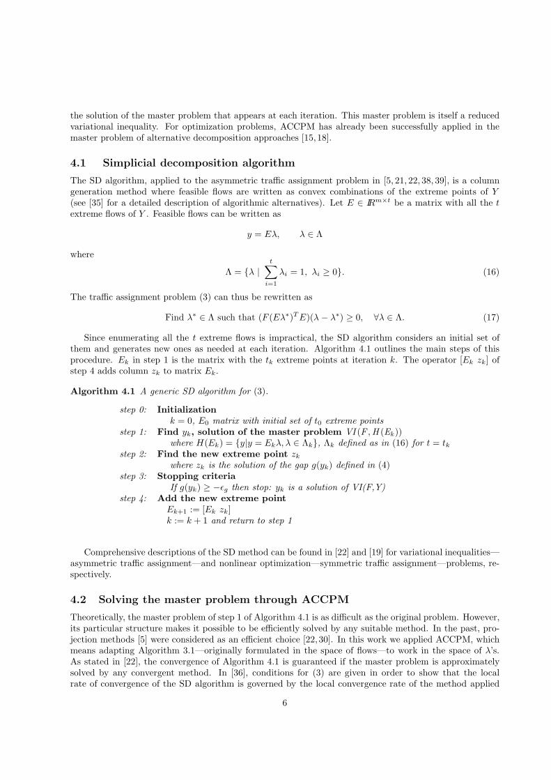
the solution of the master problem that appears at each iteration. This master problem is itself a reducedvariational inequality. For optimization problems, ACCPM has already been successfully applied in themaster problem of alternative decomposition approaches [15, 18].

4.1 Simplicial decomposition algorithm

The SD algorithm, applied to the asymmetric traffic assignment problem in [5, 21, 22, 38, 39], is a columngeneration method where feasible flows are written as convex combinations of the extreme points of Y(see [35] for a detailed description of algorithmic alternatives). Let E ∈ IRm×t be a matrix with all the textreme flows of Y . Feasible flows can be written as

y = Eλ, λ ∈ Λ

where

Λ = {λ |

t∑

i=1

λi = 1, λi ≥ 0}. (16)

The traffic assignment problem (3) can thus be rewritten as

Find λ∗ ∈ Λ such that (F (Eλ∗)T E)(λ − λ∗) ≥ 0, ∀λ ∈ Λ. (17)

Since enumerating all the t extreme flows is impractical, the SD algorithm considers an initial set ofthem and generates new ones as needed at each iteration. Algorithm 4.1 outlines the main steps of thisprocedure. Ek in step 1 is the matrix with the tk extreme points at iteration k. The operator [Ek zk] ofstep 4 adds column zk to matrix Ek.

Algorithm 4.1 A generic SD algorithm for (3).

step 0: Initialization

k = 0, E0 matrix with initial set of t0 extreme pointsstep 1: Find yk, solution of the master problem VI (F ,H (Ek ))

where H(Ek) = {y|y = Ekλ, λ ∈ Λk}, Λk defined as in (16) for t = tkstep 2: Find the new extreme point zk

where zk is the solution of the gap g(yk) defined in (4)step 3: Stopping criteria

If g(yk) ≥ −ǫg then stop: yk is a solution of VI(F,Y)step 4: Add the new extreme point

Ek+1 := [Ek zk]k := k + 1 and return to step 1

Comprehensive descriptions of the SD method can be found in [22] and [19] for variational inequalities—asymmetric traffic assignment—and nonlinear optimization—symmetric traffic assignment—problems, re-spectively.

4.2 Solving the master problem through ACCPM

Theoretically, the master problem of step 1 of Algorithm 4.1 is as difficult as the original problem. However,its particular structure makes it possible to be efficiently solved by any suitable method. In the past, pro-jection methods [5] were considered as an efficient choice [22, 30]. In this work we applied ACCPM, whichmeans adapting Algorithm 3.1—originally formulated in the space of flows—to work in the space of λ’s.As stated in [22], the convergence of Algorithm 4.1 is guaranteed if the master problem is approximatelysolved by any convergent method. In [36], conditions for (3) are given in order to show that the localrate of convergence of the SD algorithm is governed by the local convergence rate of the method applied

6

for approximate master problem resolution. ACCPM has proved to be convergent for variational inequal-ities under some monotonicity assumptions (e.g., pseudo-co-coercivity [8] and pseudo-monotonicity [17]).Therefore the procedure here described combining SD and ACCPM converges to a solution

The master problem to be solved through ACCPM at iteration k of Algorithm 4.1, denoted as VI (F ,Λk ),can thus be stated as

find λ∗ such that F (λ∗)(λ − λ∗) ≥ 0 ∀ λ ∈ Λk, where F (λ) = (F (Ekλ)T Ek), (18)

and we define yk = Ekλ∗. Algorithm 4.2 details the main steps to be performed:

Algorithm 4.2 Detail of step 1 of Algorithm 4.1 solved through ACCPM

step 1: Find yk, solution of the master problem VI (F ,H (Ek )) through (18)(i) Initialization

Find an initial interior point and set j = 0, Λ0 = Λk

(ii) Analytic center

Find an approximate analytic center λj of Λj

(iii) New cut

Λj+1 := Λj

⋂{λ | F (λj)

T λ ≤ F (λj)T λj}

(iv) Termination criterion

Compute gap g(λj) = minz∈Λk

F (λj)T (z − λj)

if g(λj) ≥ −ǫg thenyk = Ekλj and go to step 2 of Algorithm 4.1

elsej := j + 1 and return to step (ii)

Iterations of Algorithm 4.1 are named in this work “major iterations”, whereas those of Algorithm 4.2 arereferred to as “minor iterations”.

Four variants of Algorithm 4.2 will be presented for solving (18). The first two variants are not efficientand could be omitted. However, we think it is worth to give details of them to see their main differences withthe successful approaches. The first variant starts at step (i) for j = 0 from the center of the simplex whichis also the analytic center, whereas the second variant starts at step (i) for j = 0 from an infeasible point.The first and the second variants also differ in the representation of the feasible set Λk. The third variantconsiders the same representation of the feasible set as the second variant, but heuristically computes aninitial feasible point at step (i) for j = 0. The fourth variant projects the λ computed by the third variantonto the feasible set (16), which guarantees a feasible link-flow solution. For all four variants and j > 0,the last center λj−1 was used as a warm start at step (ii), performing additional primal-dual Newton stepsto recover both feasibility and centrality [8].

4.2.1 First variant

In the first variant the initial feasible set Λk, defined as in (16) considering t = tk, is represented as

Λk ={λ | AT λ ≤ c, Bλ = 1

}, (19)

where AT = −Itk∈ IRtk×tk is the minus identity matrix, c ∈ IRtk is a zero vector, and B ∈ IR1×tk is a row

vector of ones. The new inequalities computed at step (iii) of Algorithm 4.2 will be successively added tomatrix AT

j (initially AT0 = AT ). At iteration j the dimension of AT

j is (tk + j) × tk.This representation of the feasible set clearly matches (8), replacing y by λ. It can be shown (see [8]

for details) that if we solve the optimality conditions (11–15) of (10), each Newton iteration involves linearsystems with

∆ = AjS−1XAT

j and H = B∆−1BT , (20)

where S and X are diagonal positive definite matrices derived from s and x. ∆ has dimension tk × tk,independent of the number of cuts generated. The solution of the linear systems is performed by dense

7

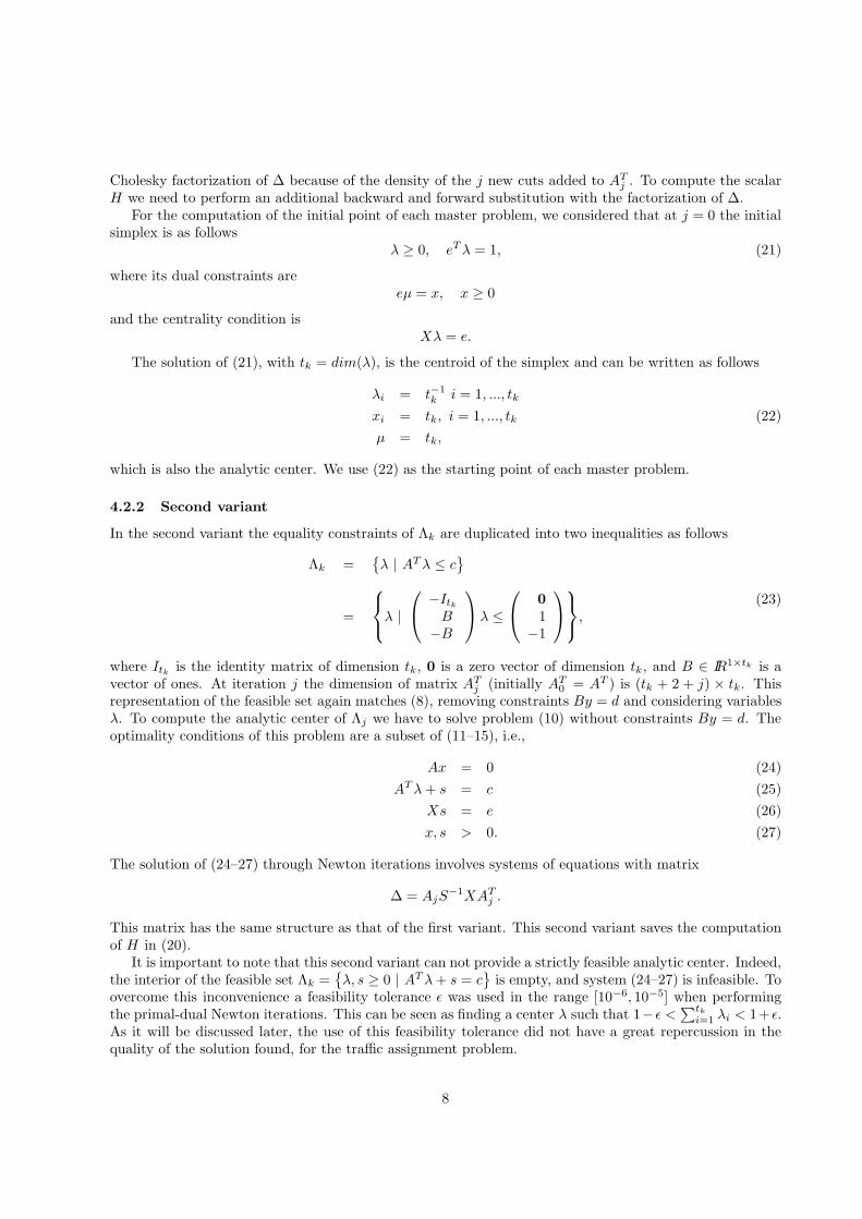
Cholesky factorization of ∆ because of the density of the j new cuts added to ATj . To compute the scalar

H we need to perform an additional backward and forward substitution with the factorization of ∆.For the computation of the initial point of each master problem, we considered that at j = 0 the initial

simplex is as followsλ ≥ 0, eT λ = 1, (21)

where its dual constraints areeµ = x, x ≥ 0

and the centrality condition isXλ = e.

The solution of (21), with tk = dim(λ), is the centroid of the simplex and can be written as follows

λi = t−1k i = 1, ..., tk

xi = tk, i = 1, ..., tk (22)

µ = tk,

which is also the analytic center. We use (22) as the starting point of each master problem.

4.2.2 Second variant

In the second variant the equality constraints of Λk are duplicated into two inequalities as follows

Λk ={λ | AT λ ≤ c

}

=

λ |

−Itk

B−B

λ ≤

0

1−1

,(23)

where Itkis the identity matrix of dimension tk, 0 is a zero vector of dimension tk, and B ∈ IR1×tk is a

vector of ones. At iteration j the dimension of matrix ATj (initially AT

0 = AT ) is (tk + 2 + j) × tk. Thisrepresentation of the feasible set again matches (8), removing constraints By = d and considering variablesλ. To compute the analytic center of Λj we have to solve problem (10) without constraints By = d. Theoptimality conditions of this problem are a subset of (11–15), i.e.,

Ax = 0 (24)

AT λ + s = c (25)

Xs = e (26)

x, s > 0. (27)

The solution of (24–27) through Newton iterations involves systems of equations with matrix

∆ = AjS−1XAT

j .

This matrix has the same structure as that of the first variant. This second variant saves the computationof H in (20).

It is important to note that this second variant can not provide a strictly feasible analytic center. Indeed,the interior of the feasible set Λk =

{λ, s ≥ 0 | AT λ + s = c

}is empty, and system (24–27) is infeasible. To

overcome this inconvenience a feasibility tolerance ǫ was used in the range [10−6, 10−5] when performingthe primal-dual Newton iterations. This can be seen as finding a center λ such that 1− ǫ <

∑tk

i=1 λi < 1+ ǫ.As it will be discussed later, the use of this feasibility tolerance did not have a great repercussion in thequality of the solution found, for the traffic assignment problem.

8

4.2.3 Third variant

The third variant also represents the feasible set by (23) and the optimality conditions of its analytic centerare (24–27). However, unlike the second variant, the starting point is heuristically obtained as

λi = 1/tk i = 1, . . . , tksi = 1/tk i = 1, . . . , tkxi = tk i = 1, . . . , tksi = ǫ i = tk + 1, tk + 2xi = 1/ǫ i = tk + 1, tk + 2,

(28)

for a fixed ǫ > 0 tolerance, where tk is the master problem dimension in the simplicial space. The abovepoint satisfies

Ax = tkeAT λ + s = c + ǫ(0T , 1, 1)T

Xs = ex, s > 0,

(29)

where 0 and e are vectors of dimension tk of, respectively, zeros and ones. Considering a feasibility toleranceof ǫ, this point satisfies the dual feasibility optimality condition (25), and it can be considered a dual ǫ-feasible starting point.

Equations (29) are approximately the optimality conditions (24–27), but for the primal feasibility.Indeed, it can be easily proved that (29)—setting ǫ = 0—are the optimality conditions of the perturbedanalytic center problem

maxλ,s

tk+2∑

i=1

ln si + tkeT λ

subject to AT λ + s = cs > 0.

(30)

(28) can thus be considered a fairly good approximation to the analytic center. In practice this variantprovided by far the best computational results.

Through the ǫ feasibility parameter of the starting point it is possible to perform a trade-off betweenthe quality of the solution and the computation time. Small values (e.g., ǫ = 10−7) provide (almost) theexact solution of (18) but large execution times. Values about 10−2 have empirically shown to provide goodenough approximate solutions very efficiently for some instances. Such large feasibility tolerances were notappropriate for the previous second variant: execution times were not reduced, even some numerical insta-bilities were found. However, in combination with the heuristically computed initial point, they providedthe fastest execution times.

The use of this ǫ feasibility parameter means that the master problem provides solutions such that∑tk

i=1 λi 6= 1 (indeed, the constraints impose 1− ǫ <∑tk

i=1 λi < 1+ ǫ). Therefore, the point yk computed inAlgorithm 4.1—which eventually will be reported as the solution of the traffic assignment problem—onlysatisfies approximately the demands for the different OD pairs. It is not difficult to bound the infeasibilitiesdue to this ǫ value by induction. Indeed, yk is computed as yk =

∑tk

i=1 λizi, zi being the solutions(extreme flows) obtained at previous iterations when computing the gaps. The extreme flows zi, i = 1, . . . , t0considered at the beginning of the algorithm are feasible, and thus NP zi = d (NP being the multicommoditynetwork matrix and d the demand vector, for all the OD pairs). Assuming that at iteration k we can boundNP zi for all extreme flow i = 1, . . . , tk computed in previous iteration by d(1− ǫ)k−1 < NP zi < d(1+ ǫ)k−1,then, since NP yk =

∑tk

i=1 λiNP zi, we have d(1 − ǫ)k < NP yk < d(1 + ǫ)k. From the computational resultsof Section 5, the number of major iterations k is in general not very large. Relative perturbations canthen be made arbitrarily small (e.g, ǫ = 10−7 will provide in practice a feasible solution). The ǫ valuecan thus be viewed as a relative feasibility tolerance. In this sense, we can state that we are solving atraffic assignment problem with slightly perturbed demands at the OD pairs. Moreover, in practice ODdemands are approximations of real unknown values, the error in the data likely being higher that theinfeasibilities incurred by the ǫ value considered in this algorithm. In addition, we empirically observed

9

that the patterns of flows of the approximate solution for such a large value as ǫ = 10−2 are similar to thosereported as optimal in Section 5 using, for asymmetric problems, a very small value —ǫ = 10−7— with thisthird variant, and the code of references [29, 30]; and for symmetric problems, in addition to previous twoapproaches, the Bar-Gera origin based algorithm [3]. This third variant can thus be seen as a fast methodfor computing approximations of the main patterns of flows in the traffic assignment problem. Moreover,the balance between the quality of the solution and the performance through the ǫ feasibility parametermakes the method a versatile tool. As a drawback, while departing from a primal feasible scheme, the primalgap function can theoretically not be computed, since it is defined from a current feasible point that it isnot available in this third version. A pseudo-gap has to be introduced (computed from the current slightlyinfeasible point) in order to present computational results. The monitoring of the global SD algorithm isalso affected and hence the computational results when using the third ACCPM variant and comparing itto the other variants or the original RSDVI implementation should be considered with caution, if a largeǫ value is used. For small ǫ values, the results obtained with this third version are comparable to those ofother approaches.

4.2.4 Fourth variant

In this variant the solution obtained by the third one is projected onto the feasible set (16). The newprojected point is used for the calculation of a pattern of feasible link-flows.

Let λ be the solution obtained in the third variant, and consider the projection matrix onto the feasibleset (16)

P =

(I −

eet

n

).

The fourth variant returns as solution of the master problem the feasible point λ = P λ + e/n:

λ = λ + e

(1 − etλ

n

).

The feasible link-flows used at step 2 of Algorithm 4.1, which eventually will be reported as the solution, arecomputed through the above point. Observe that it is possible to use other projection operators, like thatobtained with the norm weighted by the diagonal of the Jacobian matrix at the current point. In this work,only a two-norm projection has been tested, but the good results make a subject of future development thestudy of adapted projection norms to recover feasibility.

This fourth variant leads to a competitive approach for the global asymmetric traffic equilibrium prob-lem (3) in a SD scheme. Since SD is a primal feasible algorithm, theoretically, the overall procedurebecomes consistent and the primal gap function can be fully applied to monitor the progress and eventualconvergence. It solves the main drawback of the third variant, while still being competitive.

5 Computational experience

The four ACCPM variants of the previous Section have been implemented in C and included in the Fortrancode RSDVI for large-scale general traffic assignment problems. Implementation details of RSDVI can befound in [29, 30], and its general trends were originally proposed in [5, 22]. That code customizes severalvariants of a restricted version of the SD algorithm. It solves the master problem through several particularprojection methods allowing the use of variable metric, which for separable problems is roughly equivalent toa second order approximation. To avoid possible convergence problems in the RSD scheme for asymmetricproblems [22], an unrestricted strategy is set for all the computational tests, i.e., no extreme flow of Ygenerated by Algorithm 4.1 is discarded for matrix E; in addition, a variable metric is considered, whichuses at each linear approximation a symmetrization of the Jacobian matrix at the current point projectedinto the current simplicial space (defined by the current working set).

10

5.1 Test problems

We considered the model for transportation networks of Sioux Falls, Winnipeg, Barcelona and Madrid.Table 1 reports the dimensions of these networks, e.g., number of nodes, links and OD node pairs. Col-umn “centroids” gives the number of nodes with nonzero demands/supplies (i.e., transport zones in theunderlying network model).

Problem Nodes Centroids Links OD pairs

Sioux Falls 48 24 124 528Barcelona 930 110 2522 7922Winnipeg 1017 154 2976 4345Madrid 2776 490 6871 26037

Table 1: Test networks dimensions

For each network of Table 1 we developed two different categories of traffic assignment instances (using aslightly improved version of the specialized routines of [30]): diagonal and asymmetric problems. Diagonalproblems involve separable cost functions (e.g., the Jacobian of the travel cost function F (y) is diagonal).The asymmetric problems were artificially built by including additional link interactions among incominglinks at junctions. The Jacobian of F (y) is asymmetric. Neither modal networks, nor modal interactionswere considered.

We used a general form of the standard BPR (Bureau of Public Roads) cost function. It provides thejourney time for each link of the network. For a diagonal problem, it can be written as

Fa(ya) = t0

(1 + α

(ya

ca

)β)

, (31)

where ca is the capacity of link a, and t0 is the travel time through this link when it is empty (zero flow).Parameters α and β were set to the standard values of, respectively, 0.15 and 4.

For real world instances, the estimation of exact asymmetric cost functions is a difficult task. We there-fore generated asymmetric problems by adding interactions between incoming links at junctions throughthe term

∑b∈Ia

wabyb. For each link a we considered the following asymmetric cost function:

Fa(y) = t0

(1 + α

(∑b∈Ia

wabyb

ca

)β)

, (32)

where Ia is the set of links interacting with link a, and wab are the weight interaction factors between links aand b, with waa = 1. Let γ =

∑b6=a wab be the asymmetry/nonmonotonicity coefficient. If γ < 1, then the

diagonal dominance of the Jacobian matrix of F is guaranteed at any point, and thus, it is positive definiteand the F mapping is strictly monotone. If γ = 0 then a symmetric and diagonal instance of the trafficassignment problem holds. For γ > 1 a nondiagonal dominant matrix is obtained and thus monotonicity ofF is not guaranteed. In general, the pattern of interactions used in the computational tests of this work ledto sparse Jacobian matrices whose asymmetric level, as defined by some authors [27], can be very high [29].

The wab weights for flows on links b interacting with the current link a are equal and proportionallycomputed in order to satisfy a preselected γ value. This versatile family of F mappings, together with otherpatterns of interactions available in the RSDVI program, were proposed and widely discussed in [29]. Thatimplementation was slightly improved in this work for the generation of the asymmetric functions.

5.2 Computational results

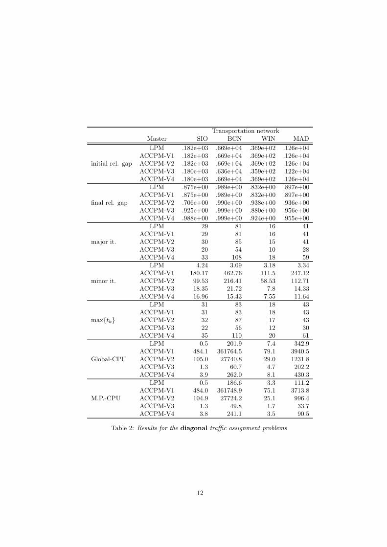
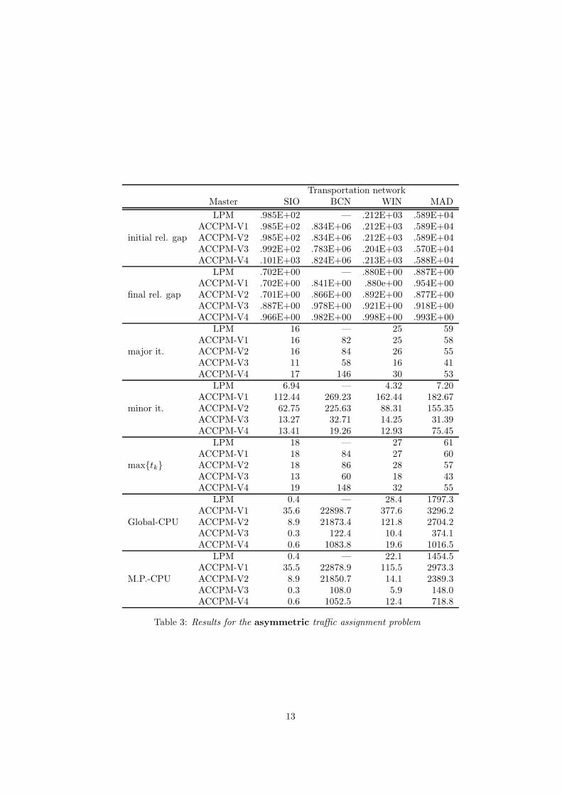
Tables 2–3 report the results obtained, respectively for, diagonal and asymmetric instances. For the asym-metric instances the asymmetric coefficient γ was set to .95. Columns “SIO”, “BCN”, “WIN” and “MAD”

11

Transportation networkMaster SIO BCN WIN MAD

LPM .182e+03 .669e+04 .369e+02 .126e+04ACCPM-V1 .182e+03 .669e+04 .369e+02 .126e+04

initial rel. gap ACCPM-V2 .182e+03 .669e+04 .369e+02 .126e+04ACCPM-V3 .180e+03 .636e+04 .359e+02 .122e+04ACCPM-V4 .180e+03 .669e+04 .369e+02 .126e+04

LPM .875e+00 .989e+00 .832e+00 .897e+00ACCPM-V1 .875e+00 .989e+00 .832e+00 .897e+00

final rel. gap ACCPM-V2 .706e+00 .990e+00 .938e+00 .936e+00ACCPM-V3 .925e+00 .999e+00 .880e+00 .956e+00ACCPM-V4 .988e+00 .999e+00 .924e+00 .955e+00

LPM 29 81 16 41ACCPM-V1 29 81 16 41

major it. ACCPM-V2 30 85 15 41ACCPM-V3 20 54 10 28ACCPM-V4 33 108 18 59

LPM 4.24 3.09 3.18 3.34ACCPM-V1 180.17 462.76 111.5 247.12

minor it. ACCPM-V2 99.53 216.41 58.53 112.71ACCPM-V3 18.35 21.72 7.8 14.33ACCPM-V4 16.96 15.43 7.55 11.64

LPM 31 83 18 43ACCPM-V1 31 83 18 43

max{tk} ACCPM-V2 32 87 17 43ACCPM-V3 22 56 12 30ACCPM-V4 35 110 20 61

LPM 0.5 201.9 7.4 342.9ACCPM-V1 484.1 361764.5 79.1 3940.5

Global-CPU ACCPM-V2 105.0 27740.8 29.0 1231.8ACCPM-V3 1.3 60.7 4.7 202.2ACCPM-V4 3.9 262.0 8.1 430.3

LPM 0.5 186.6 3.3 111.2ACCPM-V1 484.0 361748.9 75.1 3713.8

M.P.-CPU ACCPM-V2 104.9 27724.2 25.1 996.4ACCPM-V3 1.3 49.8 1.7 33.7ACCPM-V4 3.8 241.1 3.5 90.5

Table 2: Results for the diagonal traffic assignment problems

12

Transportation networkMaster SIO BCN WIN MAD

LPM .985E+02 — .212E+03 .589E+04ACCPM-V1 .985E+02 .834E+06 .212E+03 .589E+04

initial rel. gap ACCPM-V2 .985E+02 .834E+06 .212E+03 .589E+04ACCPM-V3 .992E+02 .783E+06 .204E+03 .570E+04ACCPM-V4 .101E+03 .824E+06 .213E+03 .588E+04

LPM .702E+00 — .880E+00 .887E+00ACCPM-V1 .702E+00 .841E+00 .880e+00 .954E+00

final rel. gap ACCPM-V2 .701E+00 .866E+00 .892E+00 .877E+00ACCPM-V3 .887E+00 .978E+00 .921E+00 .918E+00ACCPM-V4 .966E+00 .982E+00 .998E+00 .993E+00

LPM 16 — 25 59ACCPM-V1 16 82 25 58

major it. ACCPM-V2 16 84 26 55ACCPM-V3 11 58 16 41ACCPM-V4 17 146 30 53

LPM 6.94 — 4.32 7.20ACCPM-V1 112.44 269.23 162.44 182.67

minor it. ACCPM-V2 62.75 225.63 88.31 155.35ACCPM-V3 13.27 32.71 14.25 31.39ACCPM-V4 13.41 19.26 12.93 75.45

LPM 18 — 27 61ACCPM-V1 18 84 27 60

max{tk} ACCPM-V2 18 86 28 57ACCPM-V3 13 60 18 43ACCPM-V4 19 148 32 55

LPM 0.4 — 28.4 1797.3ACCPM-V1 35.6 22898.7 377.6 3296.2

Global-CPU ACCPM-V2 8.9 21873.4 121.8 2704.2ACCPM-V3 0.3 122.4 10.4 374.1ACCPM-V4 0.6 1083.8 19.6 1016.5

LPM 0.4 — 22.1 1454.5ACCPM-V1 35.5 22878.9 115.5 2973.3

M.P.-CPU ACCPM-V2 8.9 21850.7 14.1 2389.3ACCPM-V3 0.3 108.0 5.9 148.0ACCPM-V4 0.6 1052.5 12.4 718.8

Table 3: Results for the asymmetric traffic assignment problem

13

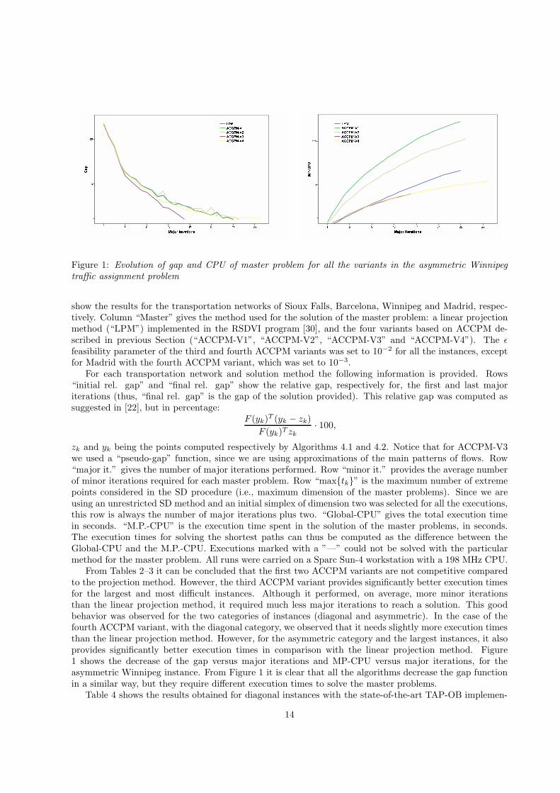
Figure 1: Evolution of gap and CPU of master problem for all the variants in the asymmetric Winnipegtraffic assignment problem

show the results for the transportation networks of Sioux Falls, Barcelona, Winnipeg and Madrid, respec-tively. Column “Master” gives the method used for the solution of the master problem: a linear projectionmethod (“LPM”) implemented in the RSDVI program [30], and the four variants based on ACCPM de-scribed in previous Section (“ACCPM-V1”, “ACCPM-V2”, “ACCPM-V3” and “ACCPM-V4”). The ǫfeasibility parameter of the third and fourth ACCPM variants was set to 10−2 for all the instances, exceptfor Madrid with the fourth ACCPM variant, which was set to 10−3.

For each transportation network and solution method the following information is provided. Rows“initial rel. gap” and “final rel. gap” show the relative gap, respectively for, the first and last majoriterations (thus, “final rel. gap” is the gap of the solution provided). This relative gap was computed assuggested in [22], but in percentage:

F (yk)T (yk − zk)

F (yk)T zk

· 100,

zk and yk being the points computed respectively by Algorithms 4.1 and 4.2. Notice that for ACCPM-V3we used a “pseudo-gap” function, since we are using approximations of the main patterns of flows. Row“major it.” gives the number of major iterations performed. Row “minor it.” provides the average numberof minor iterations required for each master problem. Row “max{tk}” is the maximum number of extremepoints considered in the SD procedure (i.e., maximum dimension of the master problems). Since we areusing an unrestricted SD method and an initial simplex of dimension two was selected for all the executions,this row is always the number of major iterations plus two. “Global-CPU” gives the total execution timein seconds. “M.P.-CPU” is the execution time spent in the solution of the master problems, in seconds.The execution times for solving the shortest paths can thus be computed as the difference between theGlobal-CPU and the M.P.-CPU. Executions marked with a ”—” could not be solved with the particularmethod for the master problem. All runs were carried on a Sparc Sun-4 workstation with a 198 MHz CPU.

From Tables 2–3 it can be concluded that the first two ACCPM variants are not competitive comparedto the projection method. However, the third ACCPM variant provides significantly better execution timesfor the largest and most difficult instances. Although it performed, on average, more minor iterationsthan the linear projection method, it required much less major iterations to reach a solution. This goodbehavior was observed for the two categories of instances (diagonal and asymmetric). In the case of thefourth ACCPM variant, with the diagonal category, we observed that it needs slightly more execution timesthan the linear projection method. However, for the asymmetric category and the largest instances, it alsoprovides significantly better execution times in comparison with the linear projection method. Figure1 shows the decrease of the gap versus major iterations and MP-CPU versus major iterations, for theasymmetric Winnipeg instance. From Figure 1 it is clear that all the algorithms decrease the gap functionin a similar way, but they require different execution times to solve the master problems.

Table 4 shows the results obtained for diagonal instances with the state-of-the-art TAP-OB implemen-

14

Instance Iterations Minor iterations final gap Obj. Global-CPU∗

Sioux Falls 12 501 1.4E-07 4231335.28 0.53 · 35 = 18.6Barcelona 77 5135 2.7E-06 3807082.05 541.6 · 35 = 18956.0Winnipeg 27 570 4.3E-08 702010.60 46.6 · 35 = 1631.0∗ original CPU time times 35, the ratio between the workstations used for executions in Tables 2 and 4

Table 4: Results for the symmetric traffic assignment problem using the origin-based algorithm

tation of Bar-Gera origin-based algorithm [3]. The particular input format of our implementation could beconverted to TAP-OB format for all the instances but for Madrid. For each instance, Table 4 reports thenumber of main and minor iterations required by TAP-OB, the final gap obtained, the optimal objectivefunction, and the CPU time required. These executions were performed on a PC with one AMD Athlon4400+ 64 bits dual core processor, which is roughly 35 times faster than the Sun-4 workstation used for theother runs. CPU times of Table 4 are affected by this ratio for the purpose of comparison. It is worth notingthat the origin-based algorithm solves the optimization problem associated to a diagonal traffic assignmentproblem, whereas our approach solves the variational inequality formulation. Therefore, although TAP-OBconsistently provides solutions with smaller final gaps, these are not directly comparable with those of Table2 because of the different formulations. For instance, for Barcelona, TAP-OB reported a solution with afinal gap of 2.7 · 10−6 while the final relative gap for ACCPM-V4 was 9.9 · 10−3 (the value in Table 2 hasbeen divided by 100 because it is a percentage). The optimization formulation of the origin-based algorithmalso explains column “Obj.” in Table 4. Indeed, it is possible to compare the objective function providedby TAP-OB and the other codes using the results of Table 5 of next Subsection for Winnipeg instance:TAP-OB obtains a solution with objective 702010.60, whereas ACCPM-V3, ACCPM-V4 and LPM reportrespectively 705277.2, 705287.0 and 705277.2 in a fraction of the time needed by TAP-OB. TAP-OB requires8 · 35 = 280 seconds to reach an objective value below 706000.0. ACCPM-V3 and ACCPM-V4 are thuscompetitive against TAP-OB to obtain approximate solutions, although, relying on a SD scheme, they cannot provide very accurate ones. Since the origin-based algorithm is based on the optimization formulation,asymmetric instances of Table 3 could not be solved with TAP-OB.

5.2.1 Analysis of the third and fourth ACCPM variant

The approximate solutions of the equilibrium problem provided by the global SD scheme while using thethird ACCPM variant and those provided under the linear projection method show similar flow patterns.In general, the discrepancies on the solutions in the link flows tend to decrease as the link flows increase.

As stated before, the ǫ feasibility parameter of the third ACCPM variant can be used to balanceefficiency and accuracy. To show this fact, we solved the diagonal Winnipeg problem for several valuesof ǫ, in order to compare solutions according to the objective function in the equivalent optimizationformulation of the equilibrium problem. Table 5 reports the results obtained, for the third ACCPM variantwith different ǫ values (columns“ACCPM-V3”), for the fourth ACCPM variant with ǫ = 10−4 and forthe linear projection method (column “LPM”). Row “Obj(y∗)” provides the objective function value ofthe equivalent optimization problem formulation. The objective value of column “LPM” is assumed tobe that of the optimal solution. Row “final rel. gap” is the gap of the solution provided. Rows “majorit.” and “minor it.” show the major and average minor iterations, respectively. Row “Global-CPU”gives the overall execution time. Clearly, the smaller the ǫ, the better the objective cost of the solutionsprovided by ACCPM-V3. On the other hand, execution times tend to considerably increase for small values.However, for ǫ = 10−2 a solution with a good enough objective value was already obtained—the relativeerror is 1.5 ·10−3—in a fraction of the time required by the fourth variant and the linear projection method.However, it is worth noting that for ACCPM-V3 and large ǫ values the objective function is being evaluatedat slightly infeasible points. For ACCPM-V4 the objective function is always evaluated at feasible points,because of the projection onto the feasible set by this fourth variant. If a feasible link-flows solution isrequired we are forced to use either the third variant with a small ǫ or the fourth variant. Although for

15

diagonal problems these feasible ACCPM variants may be outperformed by alternative procedures, theyare competitive for asymmetric instances, as shown in Table 3 and Subsection 5.2.2.

ACCPM-V3 ACCPM-V4 LPMǫ = 10−2 ǫ = 10−4 ǫ = 10−6 ǫ = 10−7 ǫ = 10−4

final rel. gap .880 .732 .832 .832 .757 .832major it. 10 16 16 16 16 16minor it. 7.8 42.87 79.18 96.5 42.75 3.18Global-CPU 4.7 22.2 46.1 61.8 22.1 7.4Obj(y∗) 704207.8 705252.4 705277.1 705277.2 705287.0 705277.2

Table 5: accuracy vs. efficiency for the diagonal Winnipeg instance

It could be argued that the good behavior of the third ACCPM variant shown in Table 5 is merely dueto the use of a greater feasibility and optimality tolerances than the linear projection method. However,the linear projection method did not perform better when such tolerances were relaxed.

5.2.2 Using different levels of asymmetry

Asymmetric instances with different levels of asymmetry were obtained by considering the cost function(32) with different weight interaction factors between links. For those instances we only compared the thirdand fourth ACCPM variants with the linear projection method.

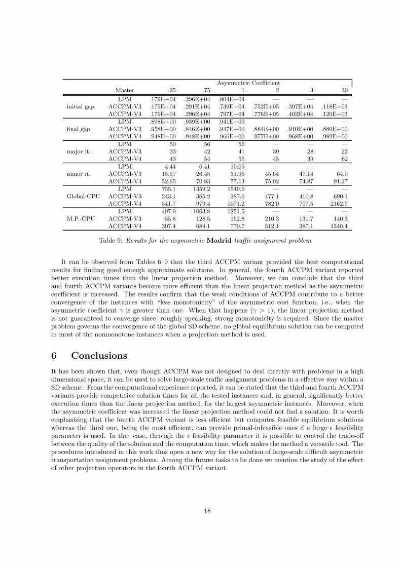
Tables 6–9 report the results obtained for, respectively, Sioux Falls, Barcelona, Winnipeg and Madridasymmetric instances. Column “Master” gives the method used for the solution of the master problem. Theǫ feasibility parameter of the third and fourth ACCPM variants was set to 10−2 for all the instances, exceptfor Madrid with the fourth ACCPM variant, which was set to 10−3, and for Winnipeg using the fourthACCPM variant, with γ = 2, 3, 10, which was set to 10−3. Columns “Asymmetric Coefficient” provide thedifferent levels of asymmetry that were tested. The information provided by the rows has the same meaningas in Tables 2 and 3.

Asymmetric CoefficientMaster .25 .75 1 2 3 10

LPM .686E+02 .109E+03 .965E+02 — — —initial gap ACCPM-V3 .676E+02 .108E+03 .964E+02 .654E+02 .468E+02 .350E+02

ACCPM-V4 .679E+02 .110E+03 .980E+02 .661E+02 .473E+02 .355E+02LPM .768E+00 .928E+00 .956E+00 — — —

final gap ACCPM-V3 .956E+00 .983E+00 .709E+00 .641E+00 .664E+00 .306E+00ACCPM-V4 .991E+00 .972E+00 .979E+00 .992E+00 .932E+00 .686+E00

LPM 20 16 15 — — —major it. ACCPM-V3 15 12 12 12 12 18

ACCPM-V4 26 20 17 17 14 21LPM 4.85 6.17 6.33 — — —

minor it. ACCPM-V3 14.8 13.25 13.75 14.25 16.58 39.61ACCPM-V4 13.53 13.1 13.58 13.7 32.5 56.0

LPM 0.5 0.4 0.4 — — —Global-CPU ACCPM-V3 0.5 0.4 0.3 0.4 0.5 4.6

ACCPM-V4 1.5 0.8 0.6 0.7 1.7 13.1LPM 0.4 0.3 0.3 — — —

M.P.-CPU ACCPM-V3 0.5 0.3 0.3 0.3 0.4 4.5ACCPM-V4 1.4 0.8 0.6 0.7 1.7 13.0

Table 6: Results for the asymmetric Sioux Falls traffic assignment problem

16

Asymmetric CoefficientMaster .25 .75 1 2 3 10

LPM .140E+05 — .110E+07 — — —initial gap ACCPM-V3 .132E+05 .733E+04 .104E+07 .827E+06 .112E+10 .138E+09

ACCPM-V4 .141E+05 .765E+04 .109e+07 .945E+06 .113E+10 .148E+09

LPM .980E+00 — .982E+00 — — —final gap ACCPM-V3 .980E+00 .982E+00 .954E+00 .808E+00 .495E+01 .969E+05

ACCPM-V4 .994E+00 .969E+00 .998e+00 .985E+00 .898E+01 .197E+05

LPM 84 — 81 — — —major it. ACCPM-V3 52 52 56 64 188 278

ACCPM-V4 105 107 127 268 241 258

LPM 4.77 — 10.82 — — —minor it. ACCPM-V3 20.17 23.55 29.03 58.7 67.2 50.1

ACCPM-V4 14.17 16 21 32.04 47.9 98.2

LPM 587.5 — 908.4 — — —Global-CPU ACCPM-V3 60.8 67.9 100.7 372.6 28655.7 121140.3

ACCPM-V4 247.0 297.8 691.3 38429.3 63413.2 212104.4

LPM 570.4 — 890.4 — — —M.P.-CPU ACCPM-V3 46.5 52.7 84.2 352.7 28609.5 121069.3

ACCPM-V4 225.2 274.7 663.5 38370.5 63356.9 212037.8

Table 7: Results for the asymmetric Barcelona traffic assignment problem

Asymmetric CoefficientMaster .25 .75 1 2 3 10

LPM .604E+02 .180E+03 .206E+03 .224E+04 — —initial gap ACCPM-V3 .581E+02 .173E+03 .198E+03 .218E+04 .401E+04 .975E+04

ACCPM-V4 .604E+02 .179E+03 .206E+03 .224E+04 .410E+04 .973E+04

LPM .725E+00 .845E+00 .926E+00 .951E+00 — —final gap ACCPM-V3 .751E+00 .879E+00 .806E+00 .916E+00 .814E+00 .999E+01

ACCPM-V4 .978E+00 .987E+00 .984E+00 .950E+00 .948E+00 .998E+02

LPM 20 23 23 41 — —major it. ACCPM-V3 13 16 18 30 53 221

ACCPM-V4 20 27 28 38 73 209

LPM 3.45 4.08 4.29 5.85 — —minor it. ACCPM-V3 8.76 12.5 13.68 27.97 57.92 76.2

ACCPM-V4 8.45 11.62 13.62 63.45 89.63 98.1

LPM 15.8 22.7 24.5 124.4 — —Global-CPU ACCPM-V3 6.9 9.8 11.8 37.7 255.9 50774.5

ACCPM-V4 10.2 16.1 18.6 151.2 1234.4 86870.6

LPM 10.7 17.2 19.0 114.7 — —M.P.-CPU ACCPM-V3 3.0 5.4 7.0 30.1 239.8 50687.8

ACCPM-V4 4.8 9.6 12.1 141.8 1213.6 86769.9

Table 8: Results for the asymmetric Winnipeg traffic assignment problem

17

Asymmetric CoefficientMaster .25 .75 1 2 3 10

LPM .179E+04 .296E+04 .804E+04 — — —initial gap ACCPM-V3 .175E+04 .291E+04 .739E+04 .752E+05 .397E+04 .118E+03

ACCPM-V4 .179E+04 .296E+04 .797E+04 .776E+05 .402E+04 .120E+03

LPM .898E+00 .939E+00 .941E+00 — — —final gap ACCPM-V3 .958E+00 .846E+00 .947E+00 .884E+00 .910E+00 .880E+00

ACCPM-V4 .948E+00 .948E+00 .966E+00 .977E+00 .968E+00 .982E+00

LPM 50 56 56 — — —major it. ACCPM-V3 33 42 41 39 28 22

ACCPM-V4 43 54 55 45 39 62

LPM 4.44 6.41 10.05 — — —minor it. ACCPM-V3 15.57 26.45 31.95 45.64 47.14 64.0

ACCPM-V4 52.65 70.83 77.13 75.02 74.87 91.27

LPM 755.1 1359.2 1549.6 — — —Global-CPU ACCPM-V3 243.1 365.2 387.0 477.1 410.8 690.1

ACCPM-V4 541.7 979.4 1071.2 782.0 707.5 2162.9

LPM 497.9 1063.8 1251.5 — — —M.P.-CPU ACCPM-V3 55.8 128.5 152.8 210.3 131.7 140.3

ACCPM-V4 307.4 684.1 770.7 512.1 387.1 1340.4

Table 9: Results for the asymmetric Madrid traffic assignment problem

It can be observed from Tables 6–9 that the third ACCPM variant provided the best computationalresults for finding good enough approximate solutions. In general, the fourth ACCPM variant reportedbetter execution times than the linear projection method. Moreover, we can conclude that the thirdand fourth ACCPM variants become more efficient than the linear projection method as the asymmetriccoefficient is increased. The results confirm that the weak conditions of ACCPM contribute to a betterconvergence of the instances with “less monotonicity” of the asymmetric cost function, i.e., when theasymmetric coefficient γ is greater than one. When that happens (γ > 1), the linear projection methodis not guaranteed to converge since, roughly speaking, strong monotonicity is required. Since the masterproblem governs the convergence of the global SD scheme, no global equilibrium solution can be computedin most of the nonmonotone instances when a projection method is used.

6 Conclusions

It has been shown that, even though ACCPM was not designed to deal directly with problems in a highdimensional space, it can be used to solve large-scale traffic assignment problems in a effective way within aSD scheme. From the computational experience reported, it can be stated that the third and fourth ACCPMvariants provide competitive solution times for all the tested instances and, in general, significantly betterexecution times than the linear projection method, for the largest asymmetric instances. Moreover, whenthe asymmetric coefficient was increased the linear projection method could not find a solution. It is worthemphasizing that the fourth ACCPM variant is less efficient but computes feasible equilibrium solutionswhereas the third one, being the most efficient, can provide primal-infeasible ones if a large ǫ feasibilityparameter is used. In that case, through the ǫ feasibility parameter it is possible to control the trade-offbetween the quality of the solution and the computation time, which makes the method a versatile tool. Theprocedures introduced in this work thus open a new way for the solution of large-scale difficult asymmetrictransportation assignment problems. Among the future tasks to be done we mention the study of the effectof other projection operators in the fourth ACCPM variant.

18

References

[1] H. Z. Aashtiani and T. L. Magnanti, “A linearization and decomposition algorithm for computingurban traffic equilibria,” in Proceedings of the IEEE Large Scale Systems Symposium, 1982, pp. 8–19.

[2] A. Auslender, Optimization. Metodes numeriques, Masson: Paris, 1976.

[3] H. Bar-Gera, “Origin-based algorithm for the traffic assignment problem,” Transportation Science,vol. 36(4), pp. 398–417, 2002.

[4] M. J. Beckmann, C. McGuire and C. Wisten, Studies in the economics of transportation, 1956.

[5] D. P. Bertsekas and E. M. Gafni, “Projection methods for variational inequalities with application tothe traffic assignment problem,” Mathematical Programming Study, vol. 17, pp. 139–159, 1982.

[6] S. Dafermos, “Traffic equilibrium and variational inequalities,” Transportation Science, vol. 14, pp. 42–54, 1980.

[7] S. Dafermos, “Relaxation algorithms for the general asymmetric traffic equilibrium problem,” Trans-portation Science, vol. 16, pp. 231–240, 1982.

[8] M. Denault and J. L. Goffin, “On a primal-dual analytic center cutting plan method for variationalinequalities,” Computational Optimization and Applications, vol. 12, pp. 127–156, 1999.

[9] F. Facchinei and J.S. Pang, Finite-Dimensional Variational Inequalities and Complementarity Prob-lems, vol. I–II, Springer:New York, 2003.

[10] M. Florian, “Nonlinear cost network models in transportation analysis,” Mathematical ProgrammingStudy, vol. 26, pp. 167–196, 1986.

[11] M. Florian and H. Spiess, “The convergence of diagonalization algorithms for asymmetric networkequilibrium problems,” Transportation Research, vol. 16B, pp. 477–483, 1982.

[12] M. Frank and P. Wolfe, “An algorithm for quadratic programming,” Naval Research Logistics Quar-terly, vol. 3, pp. 95–110, 1956.

[13] M. Fukushima, “A relaxed projection method for variational inequalities,” Mathematical Program-ming, vol. 35, pp. 58–70, 1986.

[14] M. Fukushima and T. Itoh, “A dual approach to asymmetric traffic equilibrium problems,” Mathe-matica Japonica, vol. 32, no. 5, pp. 701–721, 1987.

[15] J.-L. Goffin, J. Gondzio, R. Sarkissian and J.-P. Vial, “Solving nonlinear multicommodity problems bythe analytic center cutting plane method,” Mathematical Programming, vol. 76, pp. 131–154, 1997.

[16] J.-L. Goffin, A. Haurie and J.-P. Vial, “Decomposition and nondifferentiable optimization with theprojective algorithm,” Management Science, vol. 38-2, pp. 284–302, 1992.

[17] J.-L. Goffin, P. Marcotte and D. Zhu, “An analytic cutting plane method for pseudo-monotone varia-tional inequalities,” Operations Research Letters, vol. 20, pp. 1–6, 1997.

[18] J.-L. Goffin, R. Sarkissian and J.-P. Vial, “Using an interior point method for the master problem ina decomposition approach,” European Journal of Operational Research, vol. 101, pp. 577–587, 1997.

[19] D. W. Hearn, S. Lawphongpanich and J. A. Ventura, “Restricted simplicial decomposition: computa-tion and extensions,” Mathematical Programming Study, vol. 31, pp. 99–118, 1987.

[20] R. Katsura, M. Fukushima and T. Ibaraki, “Interior methods for nonlinear minimum cost network flowproblems,” Journal of the Operations Research Society of Japan, vol. 32, no. 2, pp. 174–199, 1989.

19

[21] T. Larsson and M. Patriksson, “Simplicial decomposition with disaggregated representation for thetraffic assignment problem,” Transportation Science , vol. 26, pp. 4–17, 1992.

[22] S. Lawphongpanich and D. W. Hearn, “Simplicial decomposition of the asymmetric traffic assignmentproblem,” Transportation Research, vol. 18B, pp. 123–133, 1984.

[23] S. Lawphongpanich and D. W. Hearn, “Restricted simplicial decomposition with application to thetraffic assignment problem,” Ricerca Operativa, vol. 38, pp. 97–120, 1986.

[24] L. J. LeBlanc, E. K. Morlok and W. P. Pierskalla, “An efficient approach to solving the road networkequilibrium traffic assignment problem,” Transportation Research, vol. 9, pp. 309–318, 1975.

[25] P. Marcotte, “A new algorithm for solving the variational inequalities with application to the trafficassignment problem,” Mathematical Programming Study, vol. 33, pp. 339–351, 1985.

[26] P. Marcotte and J.-P. Dussault, “A modified newton method for solving variational inequalities,” inProceedings of the 24th IEEE conference on Decision and Control, 1985, vol. 33, pp. 1433–1436.

[27] P. Marcotte and J. Guelat, “Adaptation of a modified newton method for solving the asymmetrictraffic equilibrium problem,” Transportation Science, vol. 22, no. 2, pp. 112–124, 1988.

[28] G.J. Minty, “On the generalization of a direct method of the calculus of variations”, Bulletin of theAmerican Mathematical Society, vol. 73, pp. 315–321, 1967.

[29] L. Montero, A Simplicial Decomposition Approach for Solving the Variational Inequality Formulation ofthe General Traffic Assignment Problem for Large Scale Networks,. PhD thesis, Universitat Politecnicade Catalunya, Barcelona, Spain, 1992.

[30] L. Montero and J. Barcelo, “A simplicial decomposition algorithm for solving the variational inequalityformulation of the general traffic assignment problem for large scale networks,” TOP, vol. 4, no. 2,pp. 225–256, 1996.

[31] Y. Nesterov and A. Nemirovskii, Interior-Point Polynomial Algorithms in Convex Programming, SIAM:Philadelphia, 1994.

[32] Y. Nesterov and J.-P. Vial, Homogeneous Analytic Center Cutting Plane Methods for Convex Problemsand Variational Inequalities, Tech. Rep. 4, Logilab, 1997.

[33] G. Newell, Traffic flow on transportation networks, MIT Press: Cambridge, 1980.

[34] S. Nguyen and C. Dupuis, “An efficient method for computing traffic equilibria in networks withasymmetric transportation costs,” Transportation Science, vol. 18, pp. 185–202, 1984.

[35] M. Patriksson, The traffic assignment problem: Models and methods, VSP B.V.: Zeist, The Nether-lands, 1994.

[36] M. Patriksson, Nonlinear programming and variational inequality problems—a unified approach,Kluwer: Dordrecht, 1998.

[37] D. Rosas, J. Castro and L. Montero, Solving the traffic assignment problem using ACCPM, Tech. Rep.DR 2002-18, Statistics and Operation Research Department: Universitat Politecnica de Catalunya,Barcelona, Spain, 2002.

[38] M. J. Smith, “The existence and calculation of traffic equilibria,” Transportation Research, vol. 17B,pp. 291–303, 1983.

[39] M. J. Smith, “An algorithm for solving asymmetric equilibrium problems with a continuous cost-flowfunction,” Transportation Research , vol. 17B, pp. 365–371, 1983.

20

[40] M. J. Smith, “Existence, uniqueness and stability of traffic equilibria,” Transportation Research,vol. 13B, pp. 295–304, 1979.

[41] M. Solodov and P. Tseng, “Modified projection-type methods for monotone variational inequalities,”SIAM Journal on Control and Optimization, vol. 34, no. 5, pp. 1814–1830, 1996.

[42] G. Sonnevend, “New algorithms in convex programming based on a notion of “centre”(for systems ofanalytic inequalities) and on rational extrapolation,” Trends in Mathematical Optimization, pp. 311–326, 1988.

[43] J. G. Wardrop, “Some theoretical aspects of road traffic research,” in Proceedings of the Institute ofCivil Engineers, Part II, 1952, vol. 1, pp. 325–378.

21