Using H2O Driverless AI

Patrick Hall, Megan Kurka & Angela Bartz

http://docs.h2o.ai

June 2020: Version 1.8.7

Using H2O Driverless AIby Patrick Hall, Megan Kurka & Angela Bartz

Published by H2O.ai, Inc.2307 Leghorn St.Mountain View, CA 94043

©2017-2020 H2O.ai, Inc. All rights reserved.

June 2020: Version 1.8.7

Photos by ©H2O.ai, Inc.

All copyrights belong to their respective owners.While every precaution has been taken in thepreparation of this book, the publisher andauthors assume no responsibility for errors oromissions, or for damages resulting from theuse of the information contained herein.

Printed in the United States of America.

Contents

1 Overview 61.1 Citation . . . . . . . . . . . . . . . . . . . . . . . . . . . . . 61.2 Have Questions? . . . . . . . . . . . . . . . . . . . . . . . . . 6

2 Why Driverless AI? 7

3 Key Features 8

4 Supported Algorithms 10

5 Installing and Upgrading Driverless AI 12

6 Launching Driverless AI 136.1 Messages . . . . . . . . . . . . . . . . . . . . . . . . . . . . . 14

7 The Datasets Page 147.1 Adding Datasets . . . . . . . . . . . . . . . . . . . . . . . . . 157.2 Dataset Details . . . . . . . . . . . . . . . . . . . . . . . . . 17

7.2.1 Dataset Details Page . . . . . . . . . . . . . . . . . . 177.2.2 Dataset Rows Page . . . . . . . . . . . . . . . . . . . 197.2.3 Modify by Recipe . . . . . . . . . . . . . . . . . . . . 197.2.4 Downloading Datasets . . . . . . . . . . . . . . . . . 20

7.3 Splitting Datasets . . . . . . . . . . . . . . . . . . . . . . . . 217.4 Visualizing Datasets . . . . . . . . . . . . . . . . . . . . . . . 22

7.4.1 The Visualization Page . . . . . . . . . . . . . . . . . 22

8 Running an Experiment 268.1 Before You Begin . . . . . . . . . . . . . . . . . . . . . . . . 268.2 New Experiment . . . . . . . . . . . . . . . . . . . . . . . . . 268.3 Completed Experiment . . . . . . . . . . . . . . . . . . . . . 308.4 Model Scores . . . . . . . . . . . . . . . . . . . . . . . . . . 31

8.4.1 Experiment Summary . . . . . . . . . . . . . . . . . . 338.5 Viewing Experiments . . . . . . . . . . . . . . . . . . . . . . 36

8.5.1 Checkpointing, Rerunning, and Retraining . . . . . . . 368.5.2 Deleting Experiments . . . . . . . . . . . . . . . . . . 39

9 Diagnosing a Model 39

10 Project Workspace 4110.1 Linking Datasets . . . . . . . . . . . . . . . . . . . . . . . . . 42

10.1.1 Selecting Datasets . . . . . . . . . . . . . . . . . . . . 4210.2 Linking Experiments . . . . . . . . . . . . . . . . . . . . . . . 43

4 | CONTENTS

10.2.1 New Experiments . . . . . . . . . . . . . . . . . . . . 4310.2.2 Checkpointing Experiments . . . . . . . . . . . . . . . 44

10.3 The Experiments Leaderboard . . . . . . . . . . . . . . . . . 4410.3.1 Leaderboard Scoring . . . . . . . . . . . . . . . . . . . 4510.3.2 Comparing Experiments . . . . . . . . . . . . . . . . . 46

10.4 Unlinking Data on a Projects Page . . . . . . . . . . . . . . . 4810.5 Deleting Projects . . . . . . . . . . . . . . . . . . . . . . . . 48

11 Interpreting a Model 4811.1 Interpret this Model button - Regular Experiments . . . . . . . 4911.2 Interpret this Model button - Time-Series Experiments . . . . 50

11.2.1 Multi-Group Time Series MLI . . . . . . . . . . . . . . 5011.2.2 Single Time Series MLI . . . . . . . . . . . . . . . . . 52

11.3 Model Interpretation - Driverless AI Models . . . . . . . . . . 5411.4 Model Interpretation - External Models . . . . . . . . . . . . . 5711.5 Understanding the Model Interpretation Page . . . . . . . . . 59

11.5.1 Summary Page . . . . . . . . . . . . . . . . . . . . . 6111.5.2 DAI Model Dropdown . . . . . . . . . . . . . . . . . . 6111.5.3 Random Forest Dropdown . . . . . . . . . . . . . . . 7711.5.4 Dashboard Page . . . . . . . . . . . . . . . . . . . . . 80

11.6 General Considerations . . . . . . . . . . . . . . . . . . . . . 8111.6.1 Machine Learning and Approximate Explanations . . . 8111.6.2 The Multiplicity of Good Models in Machine Learning . 8211.6.3 Expectations for Consistency Between Explanatory Tech-

niques . . . . . . . . . . . . . . . . . . . . . . . . . . 82

12 Viewing Explanations 83

13 Score on Another Dataset 86

14 Transform Another Dataset 86

15 The Driverless AI Scoring Pipelines 8815.1 Visualize the Scoring Pipeline . . . . . . . . . . . . . . . . . . 8815.2 Which Pipeline Should I Use? . . . . . . . . . . . . . . . . . . 9015.3 Driverless AI Standalone Python Scoring Pipeline . . . . . . . 91

15.3.1 Python Scoring Pipeline Files . . . . . . . . . . . . . . 9115.3.2 Quick Start - Recommended Method . . . . . . . . . . 9215.3.3 Quick Start - Alternative Method . . . . . . . . . . . . 9315.3.4 The Python Scoring Module . . . . . . . . . . . . . . 9615.3.5 The Scoring Service . . . . . . . . . . . . . . . . . . . 9615.3.6 Python Scoring Pipeline FAQ . . . . . . . . . . . . . . 9915.3.7 Troubleshooting Python Environment Issues . . . . . . 99

15.4 Driverless AI MLI Standalone Scoring Package . . . . . . . . . 100

CONTENTS | 5

15.4.1 MLI Python Scoring Package Files . . . . . . . . . . . 10115.4.2 Quick Start - Recommended Method . . . . . . . . . . 10215.4.3 Quick Start - Alternative Method . . . . . . . . . . . . 10215.4.4 Prerequisites . . . . . . . . . . . . . . . . . . . . . . . 10215.4.5 MLI Python Scoring Module . . . . . . . . . . . . . . 10415.4.6 K-LIME vs Shapley Reason Codes . . . . . . . . . . . 10515.4.7 MLI Scoring Service Overview . . . . . . . . . . . . . 105

15.5 Driverless AI MOJO Scoring Pipeline . . . . . . . . . . . . . . 10815.5.1 Prerequisites . . . . . . . . . . . . . . . . . . . . . . . 10815.5.2 MOJO Scoring Pipeline Files . . . . . . . . . . . . . . 10915.5.3 Quickstart . . . . . . . . . . . . . . . . . . . . . . . . 10915.5.4 Execute the MOJO from Java . . . . . . . . . . . . . 11015.5.5 MOJO Scoring Pipeline - C++ Solution . . . . . . . . 112

15.5.5.1 Downloading the Scoring Pipeline Runtimes . 112

16 Deployment 11516.1 Additional Resources . . . . . . . . . . . . . . . . . . . . . . 11616.2 Deployments Overview Page . . . . . . . . . . . . . . . . . . 11616.3 AWS Lambda Deployment . . . . . . . . . . . . . . . . . . . 116

16.3.1 Driverless AI Prerequisites . . . . . . . . . . . . . . . 11616.3.2 AWS Access Permissions Prerequisites . . . . . . . . . 11616.3.3 Deploying the Lambda . . . . . . . . . . . . . . . . . 11816.3.4 Testing the Lambda Deployment . . . . . . . . . . . . 11916.3.5 AWS Deployment Issues . . . . . . . . . . . . . . . . . 120

16.4 REST Server Deployment . . . . . . . . . . . . . . . . . . . . 12116.4.1 Prerequisites . . . . . . . . . . . . . . . . . . . . . . . 12116.4.2 Deploying on REST Server . . . . . . . . . . . . . . . 12216.4.3 Testing the REST Server Deployment . . . . . . . . . 12316.4.4 REST Server Deployment Issues . . . . . . . . . . . . 125

17 About Driverless AI Transformations 12517.1 Numeric Transformers . . . . . . . . . . . . . . . . . . . . . . 12517.2 Time Series Experiments Transformers . . . . . . . . . . . . . 12717.3 Categorical Transformers (String) . . . . . . . . . . . . . . . . 12717.4 Text Transformers (String) . . . . . . . . . . . . . . . . . . . 12917.5 Time Transformers (Date, Time) . . . . . . . . . . . . . . . . 129

18 Logs 13018.1 Sending Logs to H2O . . . . . . . . . . . . . . . . . . . . . . 133

19 References 133

20 Authors 135

6 | Overview

1 Overview

H2O Driverless AI is an artificial intelligence (AI) platform for automaticmachine learning. Driverless AI automates some of the most difficult datascience and machine learning workflows such as feature engineering, modelvalidation, model tuning, model selection and model deployment. It aims toachieve highest predictive accuracy, comparable to expert data scientists, but inmuch shorter time thanks to end-to-end automation. Driverless AI also offersautomatic visualizations and machine learning interpretability (MLI). Especiallyin regulated industries, model transparency and explanation are just as importantas predictive performance. Modeling pipelines (feature engineering and models)are exported (in full fidelity, without approximations) both as Python modulesand as pure Java standalone scoring artifacts.

Driverless AI runs on commodity hardware. It was also specifically designedto take advantage of graphical processing units (GPUs), including multi-GPUworkstations and servers such as IBM’s Power9-GPU AC922 server and theNVIDIA DGX-1 for order-of-magnitude faster training.

This document describes how to use H2O Driverless AI UI and is updatedperiodically. To view the latest Driverless AI User Guide, please go to http://docs.h2o.ai. To view an example for running the Driverless AI PythonClient, please refer to Appendix A: The Python Client in the Driverless AI UserGuide.

For more information about Driverless AI, please see https://www.h2o.ai/driverless-ai/. For a third-party review, please see https://www.infoworld.com/article/3236048/machine-learning/review-h2oai-automates-machine-learning.html.

1.1 Citation

To cite this booklet, use the following: Hall, P., Kurka, M., and Bartz, A. (Sept2018). Using H2O Driverless AI. http://docs.h2o.ai

1.2 Have Questions?

If you have questions about using Driverless AI, we recommend reviewingthe FAQ in the Driverless AI User Guide. If after reviewing the FAQ youhave additional questions, then you can post them on Stack Overflow us-ing the driverless-ai tag at http://stackoverflow.com/questions/tagged/driverless-ai.

Why Driverless AI? | 7

2 Why Driverless AI?

Over the last several years, machine learning has become an integral part ofmany organizations’ decision-making processes at various levels. With notenough data scientists to fill the increasing demand for data-driven businessprocesses, H2O.ai offers Driverless AI, which automates several time consumingaspects of a typical data science workflow, including data visualization, featureengineering, predictive modeling, and model explanation.

H2O Driverless AI is a high-performance, GPU-enabled computing platformfor automatic development and rapid deployment of state-of-the-art predictiveanalytics models. It reads tabular data from plain text sources, Hadoop, orS3 buckets and automates data visualization and building predictive models.Driverless AI targets business applications such as loss-given-default, probabilityof default, customer churn, campaign response, fraud detection, anti-money-laundering, demand forecasting, and predictive asset maintenance models. (Orin machine learning parlance: common regression, binomial classification, andmultinomial classification problems.)

How do you frame business problems in a data set for Driverless AI?

The data that is read into Driverless AI must contain one entity per row, likea customer, patient, piece of equipment, or financial transaction. That rowmust also contain information about what you will be trying to predict usingsimilar data in the future, like whether that customer in the row of data used apromotion, whether that patient was readmitted to the hospital within thirtydays of being released, whether that piece of equipment required maintenance,or whether that financial transaction was fraudulent. (In data science speak,Driverless AI requires ”labeled” data.) Driverless AI runs through your datamany, many times looking for interactions, insights, and business drivers of thephenomenon described by the provided dataset. Driverless AI can handle simpledata quality problems, but it currently requires all data for a single predictivemodel to be in the same dataset, and that dataset must have already undergonestandard ETL, cleaning, and normalization routines before being loaded intoDriverless AI.

How do you use Driverless AI results to create commercial value?

Commercial value is generated by Driverless AI in a few ways.

• Driverless AI empowers data scientists or data analysts to work on projectsfaster and more efficiently by using automation and state-of-the-artcomputing power to accomplish tasks in just minutes or hours instead ofthe weeks or months that it can take humans.

8 | Key Features

• Like in many other industries, automation leads to standardization ofbusiness processes, enforces best practices, and eventually drives downthe cost of delivering the final product - in this case a predictive model.

• Driverless AI makes deploying predictive models easy - typically a difficultstep in the data science process. In large organizations, value frompredictive modeling is typically realized when a predictive model is movedfrom a data analyst’s or data scientist’s development environment into aproduction deployment setting. In this setting, the model is running onlive data and making quick and automatic decisions that make or savemoney. Driverless AI provides both Java- and Python-based technologiesto make production deployment simpler.

Moreover, the system was designed with interpretability and transparency inmind. Every prediction made by a Driverless AI model can be explained tobusiness users, so the system is viable even for regulated industries.

Visit https://www.h2o.ai/products/h2o-driverless-ai/ to download your free21-day evaluation copy.

3 Key Features

Below are some of the key features available in Driverless AI.

Flexibility of Data and Deployment: Driverless AI works across a variety ofdata sources including Hadoop HDFS, Amazon S3, and more. Driverless AI canbe deployed everywhere including all clouds (Microsoft Azure, AWS, GoogleCloud) and on premises on any system, but it is ideally suited for systems withGPUs, including IBM Power 9 with GPUs built in.

NVIDIA GPU Acceleration: Driverless AI is optimized to take advantage ofGPU acceleration to achieve up to 40X speedups for automatic machine learning.It includes multi-GPU algorithms for XGBoost, GLM, K-Means, and more. GPUsallow for thousands of iterations of model features and optimizations.

Automatic Data Visualization (Autovis): For datasets, Driverless AI auto-matically selects data plots based on the most relevant data statistics, generatesvisualizations, and creates data plots that are most relevant from a statisticalperspective based on the most relevant data statistics. These visualizationshelp users get a quick understanding of their data prior to starting the modelbuilding process. They are also useful for understanding the composition ofvery large datasets and for seeing trends or even possible issues, such as largenumbers of missing values or significant outliers that could impact modelingresults.

Key Features | 9

Automatic Feature Engineering: Feature engineering is the secret weaponthat advanced data scientists use to extract the most accurate results fromalgorithms. H2O Driverless AI employs a library of algorithms and featuretransformations to automatically engineer new, high value features for a givendataset. Included in the interface is an easy-to-read variable importance chartthat shows the significance of original and newly engineered features.

Automatic Model Documentation: To explain models to business usersand regulators, data scientists and data engineers must document the data,algorithms, and processes used to create machine learning models. DriverlessAI provides an Autoreport (Autodoc) for each experiment, relieving the userfrom the time-consuming task of documenting and summarizing their workflowused when building machine learning models. The Autoreport includes detailsabout the data used, the validation schema selected, model and feature tuning,and the final model created. With this capability in Driverless AI, practitionerscan focus more on drawing actionable insights from the models and save weeksor even months in development, validation, and deployment process. DriverlessAI also provides a number of autodoc configuration options, giving userseven more control over output of the Autoreport.

Time Series Forecasting: Time series forecasting is one of the biggest chal-lenges for data scientists. These models address key use cases, including demandforecasting, infrastructure monitoring, and predictive maintenance. DriverlessAI delivers superior time series capabilities to optimize for almost any predictiontime window. Driverless AI incorporates data from numerous predictors, handlesstructured character data and high-cardinality categorical variables, and handlesgaps in time series data and other missing values.

NLP with TensorFlow: Text data can contain critical information to informbetter predictions. Driverless AI automatically converts short text strings intofeatures using powerful techniques like TFIDF. With TensorFlow, Driverless AIcan also process larger text blocks and build models using all available data tosolve business problems like sentiment analysis, document classification, andcontent tagging.

Automatic Scoring Pipelines: For completed experiments, Driverless AI au-tomatically generates both Python scoring pipelines and new ultra-low latencyautomatic scoring pipelines. The new automatic scoring pipeline is a uniquetechnology that deploys all feature engineering and the winning machine learningmodel in a highly optimized, low-latency, production-ready Java code that canbe deployed anywhere.

Machine Learning Interpretability (MLI): Driverless AI provides robust in-terpretability of machine learning models to explain modeling results in ahuman-readable format. In the MLI view, Driverless AI employs a host of differ-ent techniques and methodologies for interpreting and explaining the results of

10 | Supported Algorithms

its models. A number of charts are generated automatically, including K-LIME,Shapley, Variable Importance, Decision Tree Surrogate, Partial Dependence,Individual Conditional Expectation (ICE) and more. Additionally, you candownload a CSV of LIME and Shapley reasons codes from this view.

Automatic Reason Codes: In regulated industries, an explanation is oftenrequired for significant decisions relating to customers (for example, creditdenial). Reason codes show the key positive and negative factors in a model’sscoring decision in a simple language. Reasons codes are also useful in otherindustries, such as healthcare, because they can provide insights into modeldecisions that can drive additional testing or investigation.

Custom Recipe Support: Driverless AI allows you to import custom recipes forMLI algorithms, feature engineering (transformers), scorers, and configuration.You can use your custom recipes in combination with or instead of all built-in recipes. This allows you to have greater influence over the Driverless AIAutomatic ML pipeline and gives you control over the optimization choices thatDriverless AI makes.

4 Supported AlgorithmsConstant Model

A Constant Model predicts the same constant value for any input data. Theconstant value is computed by optimizing the given scorer. For example, forMSE/RMSE, the constant is the (weighted) mean of the target column. ForMAE, it is the (weighted) median. For other scorers like MAPE or customscorers, the constant is found with an optimization process. For classificationproblems, the constant probabilities are the observed priors.

A constant model is meant as a baseline reference model. If it ends up beingused in the final pipeline, a warning will be issued because that would indicate aproblem in the dataset or target column (e.g., when trying to predict a randomoutcome).

Decision Tree

A Decision Tree is a single (binary) tree model that splits the training datapopulation into sub-groups (leaf nodes) with similar outcomes. No row orcolumn sampling is performed, and the tree depth and method of growth(depth-wise or loss-guided) is controlled by hyper-parameters.

FTRL

Follow the Regularized Leader (FTRL) is a DataTable implementation ([13]) ofthe FTRL-Proximal online learning algorithm proposed in ”Ad click prediction:

Supported Algorithms | 11

a view from the trenches” ([10]). This implementation uses a hashing trickand Hogwild approach ([11]) for parallelization. FTRL can do binomial andmultinomial classification, binomial and multinomial regressions, as well asregression for continuous targets.

GLM

Generalized Linear Models (GLM) estimate regression models for outcomesfollowing exponential distributions. GLMs are an extension of traditional linearmodels. They have gained popularity in statistical data analysis due to:

• the flexibility of the model structure unifying the typical regression methods(such as linear regression and logistic regression for binary classification)

• the recent availability of model-fitting software

• the ability to scale well with large datasets

Isolation Forest

Isolation Forest is useful for identifying anomalies or outliers in data. IsolationForest isolates observations by randomly selecting a feature and then randomlyselecting a split value between the maximum and minimum values of thatselected feature. This split depends on how long it takes to separate the points.Random partitioning produces noticeably shorter paths for anomalies. When aforest of random trees collectively produces shorter path lengths for particularsamples, they are highly likely to be anomalies.

LightGBM

LightGBM is a gradient boosting framework developed by Microsoft that usestree based learning algorithms. It was specifically designed for lower memoryusage and faster training speed and higher efficiency. Similar to XGBoost, it isone of the best gradient boosting implementations available. It is also used forfitting Random Forest models inside of Driverless AI.

RuleFit

The RuleFit ([3]) algorithm creates an optimal set of decision rules by firstfitting a tree model, and then fitting a Lasso (L1-regularized) GLM model tocreate a linear model consisting of the most important tree leaves (rules).

TensorFlow

TensorFlow is an open source software library for performing high performancenumerical computation. Driverless AI includes a TensorFlow NLP recipe basedon CNN Deeplearning models.

XGBoost

12 | Installing and Upgrading Driverless AI

XGBoost is a supervised learning algorithm that implements a process calledboosting to yield accurate models. Boosting refers to the ensemble learningtechnique of building many models sequentially, with each new model attemptingto correct for the deficiencies in the previous model. In tree boosting, eachnew model that is added to the ensemble is a decision tree. XGBoost providesparallel tree boosting (also known as GBDT, GBM) that solves many datascience problems in a fast and accurate way. For many problems, XGBoost isone of the best gradient boosting machine (GBM) frameworks today.

5 Installing and Upgrading Driverless AIInstallation and upgrade steps are provided in the Driverless AI User Guide. Theinstallation steps vary based on your platform and require a license key. Contactsales@h2o.ai for information on how to purchase a Driverless AI license. Or visithttps://www.h2o.ai/download/ to obtain a free 21-day trial license.

For the best (and intended-as-designed) experience, install Driverless AI onmodern data center hardware with GPUs and CUDA support. Use Pascal orVolta GPUs with maximum GPU memory for best results. (Note the older K80and M60 GPUs available in EC2 are supported and very convenient, but not asfast.)

To simplify cloud installation, Driverless AI is provided as an AMI. To simplifylocal installation, Driverless AI is provided as a Docker image. For the best per-formance, including GPU support, use nvidia-docker. For a lower-performanceexperience without GPUs, use regular docker (with the same docker image).RPM and Tar.sh options are available for native Driverless AI installations onRedHat 7, CentOS 7, and SLES 12 operating systems. And finally, a DEBinstallation is available for Ubuntu 16.04 environments and on Windows 10using Windows Subsystem for Linux (WSL).

For native installs (rpm, deb, tar.sh), Driverless AI requires a minimum of 5GB of system memory in order to start experiments and a minimum of 5 GB ofdisk space in order to run a small experiment. Note that these limits can bechanged in the config.toml file. We recommend that you have lots of systemCPU memory (64 GB or more) and 1 TB of free disk space available.

For Docker installs, we recommend 1TB of free disk space. Driverless AI usesapproximately 38 GB. In addition, the unpacking/temp files require space onthe same Linux mount /var during installation. Once DAI runs, the mountsfrom the Docker container can point to other file system mount points.

If you are running Driverless AI with GPUs, be sure that your GPU has computecapability of at least 3.5 and at least 4GB of RAM. If these requirements arenot met, then Driverless AI will switch to CPU-only mode.

Launching Driverless AI | 13

Driverless AI supports unvalidated, none, local, Client Certificate, LDAP, mTLS,OpenID, and PAM authentication. Authentication can be configured by settingenvironment variables or via a config.toml file. Refer to the Setting EnvironmentVariables section in the User Guide.

Driverless AI also supports HDFS, S3, Azure Blob Store, BlueData DataTap,Google Cloud Storage, Google Big Query, JDBC, KDB+, Minio, and Snowflakeaccess. Support for these data sources can be configured by setting environmentvariables for the data connectors or via a config.toml file. Refer to the DataConnectors section in the User Guide for more information.

6 Launching Driverless AI

Driverless AI is tested most extensively on Chrome and Firefox. For the bestuser experience, we recommend using the latest version of Chrome. You mayencounter issues if you use other browsers or earlier versions of Chrome and/orFirefox.

1. After Driverless AI is installed and started, open a browser and navigateto <driverless-ai-host-machine>:12345.

2. The first time you log in to Driverless AI, you will be prompted to readand accept the Evaluation Agreement. You must accept the terms beforecontinuing. Review the agreement, then click I agree to these termsto continue.

3. Log in by entering unique credentials. For example:

Username: h2oaiPassword: h2oai

Note that these credentials do not restrict access to Driverless AI; they areused to tie experiments to users. If you log in with different credentials,for example, then you will not see any previously run experiments.

4. As with accepting the Evaluation Agreement, the first time you log in,you will be prompted to enter your License Key. Paste the License Keyinto the License Key entry field, and then click Save to continue. Thislicense key will be saved in the host machine’s /license folder.

Note: Contact sales@h2o.ai for information on how to purchase a Driver-less AI license.

Upon successful completion, you will be ready to add datasets and run experi-ments.

14 | The Datasets Page

6.1 Messages

A Messages menu option is available when you launch Driverless AI. Click thisto view news and upcoming events regarding Driverless AI.

7 The Datasets Page

The Datasets Overview page is the Driverless AI Home page. This shows alldatasets that have been imported. Note that the first time you log in, this listwill be empty.

The Datasets Page | 15

7.1 Adding Datasets

Driverless AI supports the following dataset file formats: arff, bin, bz2, csv, dat,feather, gz, jay, orc, parquet, pkl, tgz, tsv, txt, xls, xlsx, xz, and zip (see notesfor csv, jay, orc, and parquet below).

Notes

• CSV in UTF-16 encoding is only supported when implemented with abyte order mark (BOM). If a BOM is not present, the dataset is read asUTF-8.

• For Parquet file formats, if you select to import multiple Parquet files,those files will be imported as multiple datasets. If you select a folderof Parquet files, the folder will be imported as a single dataset. Toolslike Spark/Hive export data as multiple Parquet files that are stored in adirectory with a user-defined name. For example, if you export with SparkdataFrame.write.parquet("/data/big parquet dataset"),Spark creates a folder /data/big parquet dataset, which will containmultiple ORC or Parquet files (depending on the number of partitions inthe input dataset) and metadata. Exporting ORC files produces a similarresult.

• For ORC and Parquet file formats, you may receive a ”Failed to ingestbinary file with ORC / Parquet: lists with structs are not supported” errorwhen ingesting an ORC or Parquet file that has a struct as an elementof an array. This is because PyArrow cannot handle a struct that’s anelement of an array.

• A workaround to flatten Parquet files is provided in Sparkling Water.Refer to our Sparkling Water solution for more information.

• You can create new datasets from Python script files (custom recipes)by selecting Data Recipe URL or Upload Data Recipe from the AddDataset (or Drag & Drop) dropdown menu. If you select the DataRecipe URL option, the URL must point to either a raw file, a GitHubrepository or tree, or a local file. In addition, you can create a newdataset by modifying an existing dataset with a custom recipe. Refer tothe Modify by Recipe section below for more information. Note thatdatasets created or added from recipes will be saved as .jay files.

You can add datasets using one of the following methods:

• Drag and drop files from your local machine directly onto this page. Notethat this method currently works for files that are less than 10 GB.

or

16 | The Datasets Page

1. Click the Add Dataset or Drag and Drop button to upload or add adataset.

Notes:

• Upload File, File System, HDFS, S3, Data Recipe URL, and UploadData Recipe are enabled by default. These can be disabled byremoving them from the enabled file systems setting in theconfig.toml file.

• If File System is disabled, Driverless AI will open a local filebrowserby default.

• If Driverless AI was started with data connectors enabled for AzureBlob Store, BlueData Datatap, Google Big Query, Google CloudStorage, KDB+, Minio, Snowflake, Hive, or JDBC, then these op-tions will appear in the Add Dataset (or Drag & Drop) dropdownmenu Refer to the Data Connectors section in the Driverless AI UserGuide for more information.

• When specifying to add a dataset using Data Recipe URL, theURL must point to either a raw file, a GitHub repository or tree,or a local file. When adding or uploading datasets via recipes, thedataset will be saved as a .jay file.

Notes:

• Datasets must be in delimited text format.

The Datasets Page | 17

• Driverless AI can detect the following separators: ,l;t

• When importing a folder, the entire folder and all of its contents areread into Driverless AI as a single file.

• When importing a folder, all of the files in the folder must have thesame columns.

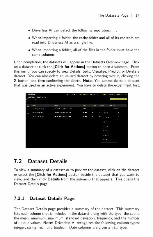
Upon completion, the datasets will appear in the Datasets Overview page. Clickon a dataset or click the [Click for Actions] button to open a submenu. Fromthis menu, you can specify to view Details, Split, Visualize, Predict, or Delete adataset. You can also delete an unused dataset by hovering over it, clicking theX button, and then confirming the delete. Note: You cannot delete a datasetthat was used in an active experiment. You have to delete the experiment first.

7.2 Dataset Details

To view a summary of a dataset or to preview the dataset, click on the datasetor select the [Click for Actions] button beside the dataset that you want toview, and then click Details from the submenu that appears. This opens theDataset Details page.

7.2.1 Dataset Details Page

The Dataset Details page provides a summary of the dataset. This summarylists each column that is included in the dataset along with the type, the count,the mean, minimum, maximum, standard deviation, frequency, and the numberof unique values. Note: Driverless AI recognizes the following column types:integer, string, real, and boolean. Date columns are given a str type.

18 | The Datasets Page

Hover over the top of a column to view a summary of the first 20 rows of thatcolumn.

To view information for a specific column, type the column name in the fieldabove the graph.

Changing a Column Type

Driverless AI also allows you to change a column type. If a column’s data typeor distribution does not match the manner in which you want the column to behandled during an experiment, changing the Logical Type can help to makethe column fit better. For example, an integer zip code can be changed into acategorical so that it is only used with categorical-related feature engineering.For Date and Datetime columns, use the Format option. To change the LogicalType or Format of a column, click on the group of square icons located to theright of the words Auto-detect. (The squares light up when you hover overthem with your cursor.) Then select the new column type for that column.

The Datasets Page | 19

7.2.2 Dataset Rows Page

To switch the view and preview the dataset, click the Dataset Rows button inthe top right portion of the UI. Then click the Dataset Overview button toreturn to the original view.

7.2.3 Modify by Recipe

The option to create a new dataset by modifying an existing dataset withcustom recipes is also available from this page. Scoring pipelines can be createdon the new dataset by building an experiment. This feature is useful when youwant to make changes to the training data that you would not need to makeon the new data you are predicting on. For example, you can change the targetcolumn from regression to classification, add a weight column to mark specifictraining rows as being more important, or remove outliers that you do not wantto model on.

20 | The Datasets Page

Click the Modify by Recipe button in the top right portion of the UI andselect from the following options:

• Data Recipe URL: Load a custom recipe from a URL to use to modifythe dataset. The URL must point to either a raw file, a GitHub repositoryor tree, or a local file.

• Upload Data Recipe: If you have a custom recipe available on yourlocal system, click this button to upload that recipe.

• Live Code: Manually enter custom recipe code to use to modify thedataset. Click the Get Preview button to preview the codes effect onthe dataset, then click Save to create a new dataset.

Notes:

• These options are enabled by default. You can disable them by removingrecipe file and recipe url from the enabled file systemsconfiguration option.

• Modifying a dataset with a recipe will not overwrite the original dataset.The dataset that is selected for modification will remain in the list ofavailable datasets in its original form, and the modified dataset will appearin this list as a new dataset.

• Changes made to the original dataset through this feature will not beapplied to new data that is scored.

7.2.4 Downloading Datasets

In Driverless AI, you can download datasets from the Datasets Overview page.

To download a dataset, click on the dataset or select the [Click for Actions]button beside the dataset that you want to download, and then select Downloadfrom the submenu that appears.

Note: The option to download datasets will not be available if the enable dataset downloadingoption is set to false when starting Driverless AI. This option can be specifiedin the config.toml file.

The Datasets Page | 21

7.3 Splitting Datasets

In Driverless AI, you can split a training dataset into test and validation datasets.

Perform the following steps to split a dataset.

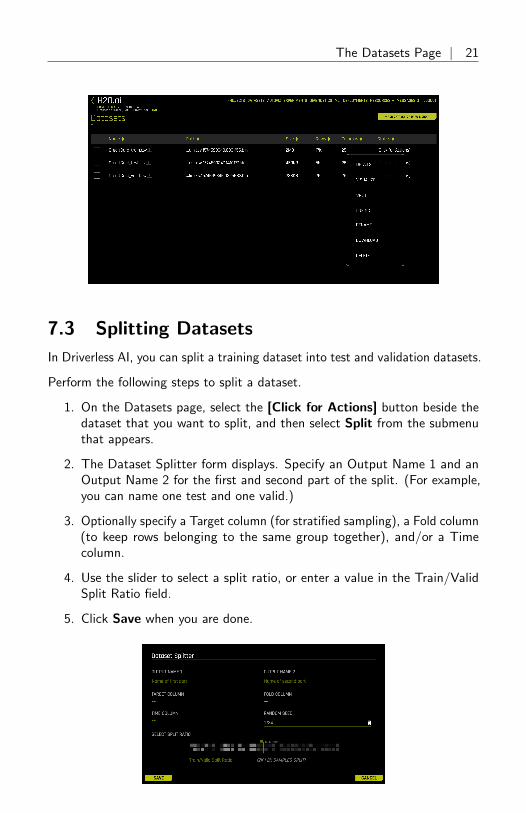
1. On the Datasets page, select the [Click for Actions] button beside thedataset that you want to split, and then select Split from the submenuthat appears.

2. The Dataset Splitter form displays. Specify an Output Name 1 and anOutput Name 2 for the first and second part of the split. (For example,you can name one test and one valid.)

3. Optionally specify a Target column (for stratified sampling), a Fold column(to keep rows belonging to the same group together), and/or a Timecolumn.

4. Use the slider to select a split ratio, or enter a value in the Train/ValidSplit Ratio field.

5. Click Save when you are done.

22 | The Datasets Page

Upon completion, the split datasets will be available on the Datasets page.

7.4 Visualizing Datasets

Perform one of the following steps to visualize a dataset:

• On the Datasets page, select the [Click for Actions] button beside thedataset that you want to view, and then click Visualize from the submenuthat appears.

• Click the Autoviz top menu link to go to the Visualizations list page,click the New Visualization button, then select or import the datasetthat you want to visualize.

7.4.1 The Visualization Page

The Visualization page shows all available graphs for the selected dataset. Notethat the graphs on the Visualization page can vary based on the information inyour dataset. You can also view and download logs that were generated duringthe visualization.

The following is a complete list of available graphs.

• Correlated Scatterplots: Correlated scatterplots are 2D plots with largevalues of the squared Pearson correlation coefficient. All possible scatter-plots based on pairs of features (variables) are examined for correlations.The displayed plots are ranked according to the correlation. Some ofthese plots may not look like textbook examples of correlation. The onlycriterion is that they have a large value of squared Pearson’s r (greaterthan .95). When modeling with these variables, you may want to leaveout variables that are perfectly correlated with others.

Note that points in the scatterplot can have different sizes. BecauseDriverless AI aggregates the data and does not display all points, the

The Datasets Page | 23

bigger the point is, the bigger number of exemplars (aggregated points)the plot covers.

• Spikey Histograms: Spikey histograms are histograms with huge spikes.This often indicates an inordinate number of single values (usually zeros)or highly similar values. The measure of ”spikeyness” is a bin frequencythat is ten times the average frequency of all the bins. You shouldbe careful when modeling (particularly regression models) with spikeyvariables.

• Skewed Histograms: Skewed histograms are ones with especially largeskewness (asymmetry). The robust measure of skewness is derived fromGroeneveld, R.A. and Meeden, G. (1984), ”Measuring Skewness andKurtosis.” The Statistician, 33, 391-399 ([6]). Highly skewed variablesare often candidates for a transformation (e.g., logging) before use inmodeling. The histograms in the output are sorted in descending orderof skewness.

• Varying Boxplots: Varying boxplots reveal unusual variability in a featureacross the categories of a categorical variable. The measure of variabil-ity is computed from a robust one-way analysis of variance (ANOVA).Sufficiently diverse variables are flagged in the ANOVA. A boxplot isa graphical display of the fractiles of a distribution. The center of thebox denotes the median, the edges of a box denote the lower and upperquartiles, and the ends of the ”whiskers” denote that range of values.Sometimes outliers occur, in which case the adjacent whisker is shortenedto the next lower or upper value. For variables (features) having only a fewvalues, the boxes can be compressed, sometimes into a single horizontalline at the median.

• Heteroscedastic Boxplots: Heteroscedastic boxplots reveal unusualvariability in a feature across the categories of a categorical variable.Heteroscedasticity is calculated with a Brown-Forsythe test: Brown, M.B. and Forsythe, A. B. (1974), ”Robust tests for equality of variances.”Journal of the American Statistical Association, 69, 364-367. Plotsare ranked according to their heteroscedasticity values. A boxplot is agraphical display of the fractiles of a distribution. The center of thebox denotes the median, the edges of a box denote the lower and upperquartiles, and the ends of the ”whiskers” denote that range of values.Sometimes outliers occur, in which case the adjacent whisker is shortenedto the next lower or upper value. For variables (features) having only a fewvalues, the boxes can be compressed, sometimes into a single horizontalline at the median.

• Biplots: A Biplot is an enhanced scatterplot that uses both points andvectors to represent structure simultaneously for rows and columns of a

24 | The Datasets Page

data matrix. Rows are represented as points (scores), and columns arerepresented as vectors (loadings). The plot is computed from the first twoprincipal components of the correlation matrix of the variables (features).You should look for unusual (non-elliptical) shapes in the points thatmight reveal outliers or non-normal distributions. And you should look forpurple vectors that are well-separated. Overlapping vectors can indicatea high degree of correlation between variables.

• Outliers: Variables with anomalous or outlying values are displayed asred points in a dot plot. Dot plots are constructed using an algorithmin Wilkinson, L. (1999). ”Dot plots.” The American Statistician, 53,276–281 ([15]). Not all anomalous points are outliers. Sometimes thealgorithm will flag points that lie in an empty region (i.e., they are notnear any other points). You should inspect outliers to see if they aremiscodings or if they are due to some other mistake. Outliers shouldordinarily be eliminated from models only when there is a reasonableexplanation for their occurrence.

• Correlation Graph: The correlation network graph is constructed from allpairwise squared correlations between variables (features). For continuous-continuous variable pairs, the statistic used is the squared Pearson corre-lation. For continuous-categorical variable pairs, the statistic is based onthe squared intraclass correlation (ICC). This statistic is computed fromthe mean squares from a one-way analysis of variance (ANOVA). Theformula is (MSbetween - MSwithin)/(MSbetween + (k - 1)MSwithin),where k is the number of categories in the categorical variable. Forcategorical-categorical pairs, the statistic is computed from Cramer’s Vsquared. If the first variable has k1 categories and the second variable hask2 categories, then a k1 x k2 table is created from the joint frequenciesof values. From this table, we compute a chi-square statistic. Cramer’sV squared statistic is then (chi-square / n) / min(k1,k2), where n is thetotal of the joint frequencies in the table. Variables with large values ofthese respective statistics appear near each other in the network diagram.The color scale used for the connecting edges runs from low (blue) tohigh (red). Variables connected by short red edges tend to be highlycorrelated.

• Parallel Coordinates Plot: A Parallel Coordinates Plot is a graph usedfor comparing multiple variables. Each variable has its own vertical axisin the plot. Each profile connects the values on the axes for a singleobservation. If the data contain clusters, these profiles will be colored bytheir cluster number.

• Radar Plot: A Radar Plot is a two-dimensional graph that is used forcomparing multiple variables. Each variable has its own axis that starts

The Datasets Page | 25

from the center of the graph. The data are standardized on each variablebetween 0 and 1 so that values can be compared across variables. Eachprofile, which usually appears in the form of a star, connects the valueson the axes for a single observation. Multivariate outliers are representedby red profiles. The Radar Plot is the polar version of the popular ParallelCoordinates plot. The polar layout enables us to represent more variablesin a single plot.

• Data Heatmap: The heatmap graphic is constructed from the transposeddata matrix. Rows of the heatmap represent variables, and columnsrepresent cases (instances). The data are standardized before displayso that small values are yellow and large values are red. The rows andcolumns are permuted via a singular value decomposition (SVD) of thedata matrix so that similar rows and similar columns are near each other.

• Recommendations: The recommendations graphic implements theTukey ladder of powers collection of log, square root, and inverse datatransformations, as well as extensions of these three transformers thathandle negative values (Yeo-Johnson). For each transformer, transforma-tions are selected by comparing the robust skewness of the transformedcolumn with the robust skewness of the original raw column. When atransformation leads to a relatively low value of skewness, it is recom-mended.

• Missing Values Heatmap: The missing values heatmap graphic isconstructed from the transposed data matrix. Rows of the heatmaprepresent variables and columns represent cases (instances). The data arecoded into the values 0 (missing) and 1 (nonmissing). Missing values arecolored red and nonmissing values are left blank (white). The rows andcolumns are permuted via a singular value decomposition (SVD) of thedata matrix so that similar rows and similar columns are near each other.

• Gaps Histogram: The gaps index is computed using an algorithm ofWainer and Schacht based on work by John Tukey. (Wainer, H. andSchacht, Psychometrika, 43, 2, 203-12.) Histograms with gaps canindicate a mixture of two or more distributions based on possible subgroupsnot necessarily characterized in the dataset.

The images on this page are thumbnails. You can click on any of the graphs toview and download a full-scale image.

26 | Running an Experiment

8 Running an Experiment

8.1 Before You Begin

This section describes how to run an experiment using the Driverless AI UI.Before you begin, it is best that you understand the available options that youcan specify. Note that only a dataset and a target column are required to bespecified, but Driverless AI provides a variety of experiment and expert settingsthat you can use to build your models. Hover over each option in the UI, orreview the Experiments section in the Driverless AI User Guide for informationabout these options.

After you have a comfortable working knowledge of these options, you are readyto start your own experiment.

8.2 New Experiment

1. Run an experiment by selecting [Click for Actions] button beside thedataset that you want to use. Click Predict to begin an experiment.

2. The Experiment Settings form displays and auto-fills with the selecteddataset. Optionally enter a custom name for this experiment. If you donot add a name, Driverless AI will create one for you.

3. Optionally specify a validation dataset and/or a test dataset.

• The validation set is used to tune parameters (models, features, etc.).If a validation dataset is not provided, the training data is used (with

Running an Experiment | 27

holdout splits). If a validation dataset is provided, training data is notused for parameter tuning - only for training. A validation datasetcan help to improve the generalization performance on shifting datadistributions.

• The test dataset is used for the final stage scoring and is thedataset for which model metrics will be computed against. Testset predictions will be available at the end of the experiment. Thisdataset is not used during training of the modeling pipeline.

These datasets must have the same number of columns as the trainingdataset. Also note that if provided, the validation set is not sampleddown, so it can lead to large memory usage, even if accuracy=1 (whichreduces the train size).

4. Specify the target (response) column. Note that not all explanatoryfunctionality will be available for multinomial classification scenarios(scenarios with more than two outcomes). When the target column isselected, Driverless AI automatically provides the target column typeand the number of rows. If this is a classification problem, then the UIshows unique and frequency statistics for numerical columns. If this is aregression problem, then the UI shows the dataset mean and standarddeviation values.

Notes Regarding Frequency:

• For data imported in versions <= 1.0.19, TARGET FREQ andMOST FREQ both represent the count of the least frequent classfor numeric target columns and the count of the most frequent classfor categorical target columns.

• For data imported in versions 1.0.20-1.0.22, TARGET FREQ andMOST FREQ both represent the frequency of the target class(second class in lexicographic order) for binomial target columns;the count of the most frequent class for categorical multinomialtarget columns; and the count of the least frequent class for numericmultinomial target columns.

• For data imported in version 1.0.23 (and later), TARGET FREQis the frequency of the target class for binomial target columns,and MOST FREQ is the most frequent class for multinomial targetcolumns.

5. The next step is to set the parameters and settings for the experiment.(Hover over each option and/or refer to the Experiment Settings section inthe Driverless AI User Guide for detailed information about these settings.)You can set the parameters individually, or you can let Driverless AI infer

28 | Running an Experiment

the parameters and then override any that you disagree with. Note thatDriverless AI will automatically infer the best settings for Accuracy, Time,and Interpretability and provide you with an experiment preview based onthose suggestions. If you adjust these knobs, the experiment preview willautomatically update based on the new settings.

Expert settings (optional):

Optionally specify additional expert settings for the experiment. Refer tothe Expert Settings section in the Driverless AI User Guide for detailedinformation about these settings. Note that the default values for theseoptions are derived from the environment variables in the config.toml file.

Additional settings (optional):

• Classification or Regression button. Driverless AI automaticallydetermines the problem type based on the response column. Thoughnot recommended, you can override this setting by clicking thisbutton.

• Reproducible: Click this button to build this with a random seed.

• Enable GPUs: Specify whether to enable GPUs. (Note that thisoption is ignored on CPU-only systems.)

6. Click Launch Experiment to start the experiment.

The experiment launches with a randomly generated experiment name.You can change this name at anytime during or after the experiment.Mouse over the name of the experiment to view an edit icon, then typein the desired name.

As the experiment runs, a running status displays in the upper middle por-tion of the UI. First Driverless AI figures out the backend and determines

Running an Experiment | 29

whether GPUs are running. Then it starts parameter tuning, followed byfeature engineering. Finally, Driverless AI builds the scoring pipeline.

In addition to the status, the UI also displays:

• Details about the dataset.

• The iteration data (internal validation) for each cross validation foldalong with the specified scorer value. Click on a specific iterationor drag to view a range of iterations. Double click in the graph toreset the view.

• The variable importance values. To view variable importance fora specific iteration, just select that iteration in the Iteration Datagraph. The Variable Importance list will automatically update toshow variable importance information for that iteration. Hover overan entry to view more info. Note: When hovering over an entry,you may notice the term ”Internal[...] specification.” This label isused for features that do not need to be translated/explained andensures that all features are uniquely identified.

• CPU/Memory information including Notifications, Logs, and Traceinfo. (Note that Trace is used for development/debugging and toshow what the system is doing at that moment.)

For classification problems, the lower right section includes a togglebetween an ROC curve, Precision-Recall graph, Lift chart, Gains chart,Kolmogorov-Smirnov chart, and GPU Usage information (if GPUs areavailable). For regression problems, the lower right section includes atoggle between a Residuals chart, an Actual vs. Predicted chart, andGPU Usage information (if GPUs are available). Refer to the ExperimentGraphs section in the User Guide for more information about these graphs.

Upon completion, an Experiment Summary section will populate in thelower right section.

You can stop experiments that are currently running. Click the Finishbutton to stop the experiment. This jumps the experiment to the endand completes the ensembling and the deployment package. You canalso click Abort to terminate the experiment. (You will be prompted toconfirm the abort.) Aborted experiments will display on the Experimentspage as Failed. You can restart aborted experiments by clicking the rightside of the experiment, then selecting Restart from Last Checkpoint.This will start a new experiment based on the aborted one. Alternatively,you can started a new experiment based on the aborted one by selectingNew Model with Same Params.

30 | Running an Experiment

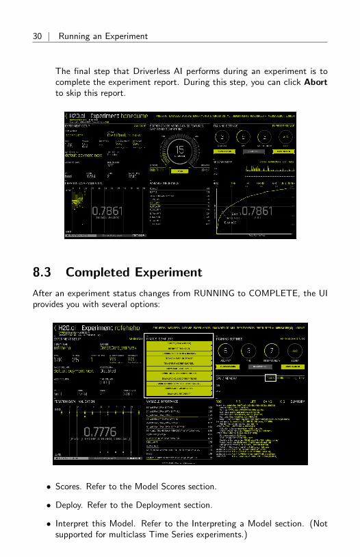
The final step that Driverless AI performs during an experiment is tocomplete the experiment report. During this step, you can click Abortto skip this report.

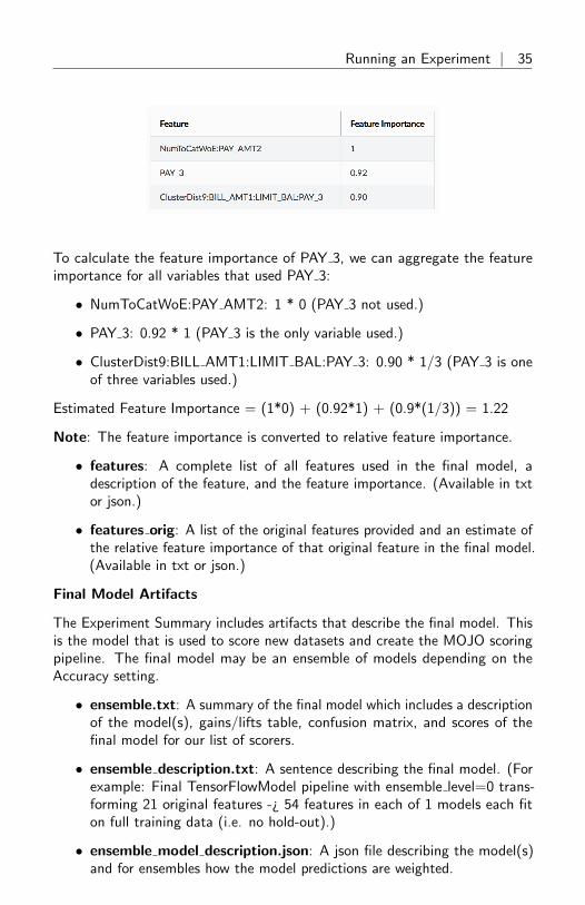
8.3 Completed Experiment

After an experiment status changes from RUNNING to COMPLETE, the UIprovides you with several options:

• Scores. Refer to the Model Scores section.

• Deploy. Refer to the Deployment section.

• Interpret this Model. Refer to the Interpreting a Model section. (Notsupported for multiclass Time Series experiments.)

Running an Experiment | 31

• Diagnose Model on New Dataset. Refer to the Diagnosing a Modelsection.

• Score on Another Dataset. Refer to the Score on Another Dataset section.

• Transform Another Dataset. Refer to the Transform Another Datasetsection. (Not available for time series experiments.)

• Download Predictions dropdown:

– Training Holdout Predictions. In csv format, available if a validationset was NOT used.

– Validation Set Predictions. In csv format, available if a validationset was used.

– Test Set Predictions. In csv format, available if a test dataset isused.

• Download Python Scoring Pipeline. A standalone Python scoring pipelinefor H2O Driverless AI.

• Build MOJO Scoring Pipeline. A standalone Model Object, Optimizedscoring pipeline. (Not available for TensorFlow, RuleFit, or FTRL models.)

• Download Experiment Summary. A zip file containing the following:

– A summary of the experiment

– The experiment features along with their relative importance

– Ensemble information

– An experiment preview

– Word version of an auto-generated report for the experiment

– A target transformations tuning leaderboard

– A tuning leaderboard

• Download Logs

8.4 Model Scores

You can view detailed information about model scores after an experiment iscomplete by clicking on the Scores option.

32 | Running an Experiment

The Model Scores page that opens includes the following tables:

• Model and feature tuning leaderboard: This leaderboard shows scoringinformation based on the scorer that was selected in the experiment. Thisinformation is also available in the tuning leaderboard.json file of theexperiment summary. You can download that file directly from the bottomof this table.

• Final pipeline scores across cross-validation folds and models: Thistable shows the final pipeline scores across cross-validation folds andmodels. Note that if Constant Model was enabled (default), then thatmodel is added in this table as a baseline (reference) only and willbe dropped in most cases. This information is also included in theensemble base learner fold scores.json file of the experiment summary.You can download that file directly from a link at the bottom of thistable.

Running an Experiment | 33

• Pipeline Description: This shows how the final Stacked Ensemblepipeline was calculated. This information is also included in the en-semble model description.json file of the experiment summary. Youcan download that file directly from a link at the bottom of this table.

• Final Ensemble Scores: This shows the final scores for each scorer in DAI.If a custom scorer was used in the experiment, that scorer will also appearhere. This information is also included in the ensemble scores.json fileof the experiment summary. You can download that file directly from alink at the bottom of this table.

8.4.1 Experiment Summary

An experiment summary is available for each completed experiment. Click theDownload Experiment Summary button to download theh2oai experiment summary <experiment>.zip file.

The files within the experiment summary zip provide textual explanations of thegraphical representations that are shown on the Driverless AI UI. For example,the preview.txt file provides the same information that was included on theUI before starting the experiment; the summary.txt file provides the samesummary that appears in the lower-right portion of the UI for the experiment;the features.txt file provides the relative importance values and descriptionsfor the top features.

34 | Running an Experiment

Experiment Report

A report file is included in the experiment summary. This report provides insightinto the training data and any detected shifts in distribution, the validationschema selected, model parameter tuning, feature evolution and the final set offeatures chosen during the experiment.

• report.docx: The report available in Word format

Experiment Overview Artifacts

The Experiment Summary contains artifacts that provide overviews of theexperiment.

• preview.txt: Provides a preview of the experiment. (This is the sameinformation that was included on the UI before starting the experiment.)

• summary.txt: Provides the same summary that appears in the lower-rightportion of the UI for the experiment.

Tuning Artifacts

During the Driverless AI experiment, model tuning is performed to determinedthe optimal algorithm and parameter settings for the provided dataset. Forregression problems, target tuning is also performed to determine the bestway to represent the target column (i.e. does taking the log of the targetcolumn improve results). The results from these tuning steps are available inthe Experiment Summary.

• tuning leaderboard: A table of the model tuning performed along withthe score generated from the model and training time. (Available in txtor json.)

• target transform tuning leaderboard.txt: A table of the transformsapplied to the target column along with the score generated from themodel and training time. (This will be empty for binary and multiclassuse cases.)

Features Artifacts

Driverless AI performs feature engineering on the dataset to determine theoptimal representation of the data. The top features used in the final modelcan be seen in the GUI. The complete list of features used in the final model isavailable in the Experiment Summary artifacts.

The Experiment Summary also provides a list of the original features and theirestimated feature importance. For example, given the features in the finalDriverless AI model, we can estimate the feature importance of the originalfeatures.

Running an Experiment | 35

To calculate the feature importance of PAY 3, we can aggregate the featureimportance for all variables that used PAY 3:

• NumToCatWoE:PAY AMT2: 1 * 0 (PAY 3 not used.)

• PAY 3: 0.92 * 1 (PAY 3 is the only variable used.)

• ClusterDist9:BILL AMT1:LIMIT BAL:PAY 3: 0.90 * 1/3 (PAY 3 is oneof three variables used.)

Estimated Feature Importance = (1*0) + (0.92*1) + (0.9*(1/3)) = 1.22

Note: The feature importance is converted to relative feature importance.

• features: A complete list of all features used in the final model, adescription of the feature, and the feature importance. (Available in txtor json.)

• features orig: A list of the original features provided and an estimate ofthe relative feature importance of that original feature in the final model.(Available in txt or json.)

Final Model Artifacts

The Experiment Summary includes artifacts that describe the final model. Thisis the model that is used to score new datasets and create the MOJO scoringpipeline. The final model may be an ensemble of models depending on theAccuracy setting.

• ensemble.txt: A summary of the final model which includes a descriptionof the model(s), gains/lifts table, confusion matrix, and scores of thefinal model for our list of scorers.

• ensemble description.txt: A sentence describing the final model. (Forexample: Final TensorFlowModel pipeline with ensemble level=0 trans-forming 21 original features -¿ 54 features in each of 1 models each fiton full training data (i.e. no hold-out).)

• ensemble model description.json: A json file describing the model(s)and for ensembles how the model predictions are weighted.

36 | Running an Experiment

• ensemble model params.json: A json file decribing the parameters ofthe model(s).

• ensemble scores.json: The scores of the final model for our list ofscorers.

• ensemble confusion matrix: The confusion matrix for the internal vali-dation and test data if test data is provided.

• ensemble confusion matrix stats test.json: Confusion matrix statis-tics on the test data. (Only available if test data provided)

• ensemble gains: The lift and gains table for the internal validation andtest data if test data is provided. (Visualization of lift and gains can beseen in the UI.)

8.5 Viewing Experiments

The upper-right corner of the Driverless AI UI includes an Experiments link.

Click this link to open the Experiments page. From this page, you can renamean experiment, view previous experiments, begin a new experiment, rerun anexperiment, and delete an experiment.

8.5.1 Checkpointing, Rerunning, and Retraining

In Driverless AI, you can retry an experiment from the last checkpoint, youcan run a new experiment using an existing experiment’s settings, and you canretrain an experiment’s final pipeline.

Running an Experiment | 37

Checkpointing Experiments

In real-world scenarios, data can change. For example, you may have a modelcurrently in production that was built using 1 million records. At a later date,you may receive several hundred thousand more records. Rather than buildinga new model from scratch, Driverless AI includes H2O.ai Brain, which enablescaching and smart re-use of prior models to generate features for new models.

You can configure one of the following Brain levels in the experiment’s ExpertSettings.

• Level -1: Dont use any brain cache

• Level 0: Dont use any brain cache but still write to cache

• Level 1: Smart checkpoint if an old experiment id is passed in (for example,via running resume one like this in the GUI)

• Level 2: Smart checkpoint if the experiment matches all column names,column types, classes, class labels, and time series options identically.(default)

• Level 3: Smart checkpoint like level 1, but for the entire population. Tuneonly if the brain population is of insufficient size.

• Level 4: Smart checkpoint like level 2, but for the entire population. Tuneonly if the brain population is of insufficient size.

• Level 5: Smart checkpoint like level 4, but will scan over the entire braincache of populations (starting from resumed experiment if chosen) inorder to get the best scored individuals.

If you chooses Level 2 (default), then Level 1 is also done when appropriate.

38 | Running an Experiment

To make use of smart checkpointing, be sure that the new data has:

• The same data column names as the old experiment

• The same data types for each column as the old experiment. (This won’tmatch if, e.g,. a column was all int and then had one string row.)

• The same target as the old experiment

• The same target classes (if classification) as the old experiment

• For time series, all choices for intervals and gaps must be the same

When the above conditions are met, then you can:

• Start the same kind of experiment, just rerun for longer.

• Use a smaller or larger data set (i.e. fewer or more rows).

• Effectively do a final ensemble re-fit by varying the data rows and startingan experiment with a new accuracy, time=1, and interpretability. Checkthe experiment preview for what the ensemble will be.

• Restart/Resume a cancelled, aborted, or completed experiment

To run smart checkpointing on an existing experiment, click the right side of theexperiment that you want to retry, then select Restart from Last Checkpoint.The experiment settings page opens. Specify the new dataset. If desired, youcan also change experiment settings, though the target column must be thesame. Click Launch Experiment to resume the experiment from the lastcheckpoint and build a new experiment.

The smart checkpointing continues by adding a prior model as another modelused during tuning. If that prior model is better (which is likely if it was run formore iterations), then that smart checkpoint model will be used during featureevolution iterations and final ensemble.

Notes:

• Driverless AI does not guarantee exact continuation, only smart continua-tion from any last point.

• The directory where the H2O.ai Brain meta model files are stored istmp/H2O.ai brain. In addition, the default maximum brain size is20GB. Both the directory and the maximum size can be changed in theconfig.toml file.

Rerunning Experiments

To run a new experiment using an existing experiment’s settings, click theright side of the experiment that you want to use as the basis for the newexperiment, then select New Model with Same Params. This opens the

Diagnosing a Model | 39

experiment settings page. From this page, you can rerun the experiment usingthe original settings, or you can specify to use new data and/or specify differentexperiment settings. Click Launch Experiment to create a new experimentwith the same options.

Retrain Final Pipeline

To retrain an experiment’s final pipeline, click the right side of the experimentthat you want to use as the basis for the new experiment, then select RetrainFinal Pipeline. This opens the experiment settings page with the same settingsas the original experiment except that Time is set to 0. This retrain mode isequivalent to setting feature brain level 3 with time 0 (no tuning or featureevolution iterations).

8.5.2 Deleting Experiments

To delete an experiment, hover over the experiment that you want to delete.An ”X” option displays. Click this to delete the experiment. A confirmationmessage will display asking you to confirm the delete. Click OK to delete theexperiment or Cancel to return to the experiments page without deleting.

9 Diagnosing a Model

The Diagnosing Model on New Dataset option allows you to view modelperformance for multiple scorers based on existing model and dataset.

On the completed experiment page, click the Diagnose Model on NewDataset button.

Notes:

• You can also diagnose a model by selecting Diagnostic from the topmenu, then selecting an experiment and test dataset.

• The Model Diagnostics page also automatically populates with any ex-periments that were scored from the Project Leaderboard on the Projectspage.

40 | Diagnosing a Model

Select a dataset to use when diagnosing this experiment. At this point, DriverlessAI will begin calculating all available scores for the experiment.

When the diagnosis is complete, it will be available on the Model Diagnosticspage. Click on the new diagnosis. From this page, you can download predictions.You can also view scores and metric plots. The plots are interactive. Click agraph to enlarge. In the enlarged view, you can hover over the graph to viewdetails for a specific point. You can also download the graph.

Classification metric plots include the following graphs:

• ROC Curve

• Precision-Recall Curve

• Cumulative Gains

• Lift Chart

• Kolmogorov-Smirnov Chart

• Confusion Matrix

Regression metric plots include the following graphs:

• Actual vs Predicted

Project Workspace | 41

• Residual Plot with LOESS curve

• Residual Histogram

10 Project Workspace

Driverless AI provides a Project Workspace for managing datasets and exper-iments related to a specific business problem or use case. Whether you aretrying to detect fraud or predict user retention, datasets and experiments canbe stored and saved in the individual projects. A Leaderboard on the Projectspage allows you to easily compare performance and results and identify the bestsolution for your problem.

To create a Project Workspace:

1. Click the Projects option on the top menu.

2. Click New Project.

3. Specify a name for the project and provide a description.

4. Click Create Project. This creates an empty Project page.

From the Projects page, you can link datasets and/or experiments, and you canrun new experiments. When you link an existing experiment to a Project, thedatasets used for the experiment will automatically be linked to this project (ifnot already linked).

42 | Project Workspace

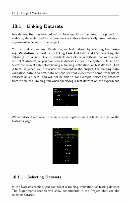
10.1 Linking Datasets

Any dataset that has been added to Driverless AI can be linked to a project. Inaddition, datasets used for experiments are also automatically linked when anexperiment is linked to the project.

You can link a Training, Validation, or Test dataset by selecting the Train-ing, Validation, or Test tab, clicking Link Dataset, and then selecting thedataset(s) to include. The list available datasets include those that were addedon :ref:‘Datasets‘, or you can browse datasets in your file system. Be sure toselect the correct tab before linking a training, validation, or test dataset. Thisis because, when you run a new experiment in the project, the training data,validation data, and test data options for that experiment come from list ofdatasets linked here. You will not be able to, for example, select any datasetsfrom within the Training tab when specifying a test dataset on the experiment.

When datasets are linked, the same menu options are available here as on theDatasets page.

10.1.1 Selecting Datasets

In the Datasets section, you can select a training, validation, or testing dataset.The Experiments section will show experiments in the Project that use theselected dataset.

Project Workspace | 43

10.2 Linking Experiments

Existing experiments can be selected and linked to a Project. Additionally, youcan run a new experiment or checkpointing an existing experiment from thispage, and those experiments will automatically be linked to this Project.

Link an existing experiment to the project by clicking Link Experiment andthen selecting the experiment(s) to include. When you link experiments, thedatasets used to create the experiments are also automatically linked.

10.2.1 New Experiments

When experiments are run from within a Project, only linked datasets can beused.

1. Click the New Experiment link to begin a new experiment.

2. Select your training data and optionally your validation and/or testingdata.

3. Specify your desired experiment settings, and then click Launch Experi-ment.

As the experiment is running, it will be listed at the top of the ExperimentsLeaderboard until it is completed. It will also be available on the Experimentspage.

44 | Project Workspace

10.2.2 Checkpointing Experiments

When experiments are linked to a Project, the same checkpointing options forexperiments are available here as on the Experiments page.

10.3 The Experiments Leaderboard

When attempting to solve a business problem, a normal workflow will includerunning multiple experiments, either with different/new data or with a varietyof settings, and the optimal solution can vary for different users and/or businessproblems. For some users, the model with the highest accuracy for validationand test data could be the most optimum one. Other users might be willingto make an acceptable compromise on the accuracy of the model for a modelwith greater performance (faster prediction). For some, it could also mean howquickly the model could be trained with acceptable levels of accuracy. TheExperiments Leaderboard makes it easy for you to find the best solution foryour business problem.

The Leaderboard is organized by showing running experiments first, then com-pleted experiments (sorted by validation score by default), then canceled experi-ments. You can change the sorting of completed experiments by selecting thesort dropdown menu.

Hover over experiments in the Leaderboard to view additional information aboutthe experiment, including the problem type, datasets used, and the targetcolumn.

Project Workspace | 45

10.3.1 Leaderboard Scoring

The Leaderboard allows you to view scoring information for a variety of scorers.You can change the scorer used by clicking the Scorer link and then selectinga scorer.

Experiments linked to projects do not automatically include a test score. Toview Test Scores in the Leaderboard, you must first complete the scoring step fora particular dataset and experiment combination. Without the scoring step, noscoring data is available to populate in the Test Score and Score Time columnsof the Leaderboard. Experiments that do not include a test score or that havean invalid scorer (for example, if the R2 scorer is selected for classificationexperiments) show N/A in the Leaderboard. Also, if None is selected for thescorer, then all experiments will show N/A.

To score the experiment:

1. Click Select Scoring Dataset at the top of the Experiments list andselect a linked Test Dataset or a test dataset available on the file system.

2. Select the model or models that you want to score.

3. Click the Select Scorer button at the top of the Experiments list andselect a scorer.

46 | Project Workspace

4. Click the Score n Items button.

Notes:

• If an experiment has already scored a dataset, it will not score it again.The scoring step is deterministic, so for a particular scorer dataset andexperiment combination, the score will be same regardless of how manytimes you repeat it.

• The scorer dataset absolutely needs to have all the columns that areexpected by the various experiments you are scoring it on. However, thecolumns of the scorer dataset need not be exactly the same as inputfeatures expected by the experiment. There can be additional columnsin the scorer dataset. If these columns were not used for training, theywill be ignored. This feature gives you the ability to train experimentson different training datasets (i.e., having different features), and if youhave an ”uber test dataset” that includes all these feature columns, thenyou can use the same dataset to score these experiments.

• You will notice a Score Time in the Experiments Leaderboard. Thisvalues shows the total time (in seconds) that it took for calculating theexperiment scores for all applicable scorers for the experiment type. Thisis valuable to users who need to estimate the runtime performance of anexperiment.

10.3.2 Comparing Experiments

You can compare two or three experiments and view side-by-side detailedinformation about each.

1. Click the Select button at the top of the Leaderboard and select eithertwo or three experiments that you want to compare. You cannot comparemore than three experiments.

2. Click the Compare n Items button.

Project Workspace | 47

This opens the Compare Experiments page. This page includes theexperiment summary for each experiment as well as metric plots. Themetric plots vary depending on whether this is a classification or regressionexperiment.

For classification experiments, this page includes:

• Variable Importance list

• Confusion Matrix

• ROC Curve

• Precision Recall Curve

• Lift Chart

• Gains Chart

• Kolmogorov-Smirnov Chart

For regression experiments, this page includes:

• Variable Importance list

• Actual vs. Predicted Graph

48 | Interpreting a Model

10.4 Unlinking Data on a Projects Page

Unlinking datasets and/or experiments does not delete that data from DriverlessAI. The datasets and experiments will still be available on the Datasets andExperiments pages.

• Unlink a dataset by clicking on the dataset and selecting Unlink fromthe menu. textbfNote: You cannot unlink datasets that are tied toexperiments in the same project.

• Unlink an experiment by clicking on the experiment and selecting Unlinkfrom the menu. Note that this will not automatically unlink datasets thatwere tied to the experiment.

10.5 Deleting Projects

To delete a project, click the Projects option on the top menu to open themain Projects page. Hover over the project that you want to delete and clickthe red X button.

Note that deleting projects does not delete datasets and experiments fromDriverless AI. Any datasets and experiments from deleted projects will still beavailable on the Datasets and Experiments pages.

11 Interpreting a ModelDriverless AI provides robust interpretability of machine learning models toexplain modeling results in a human-readable format. In the Machine LearningInterpetability (MLI) view, Driverless AI employs a host of different techniquesand methodologies for interpreting and explaining the results of its models.A number of charts are generated automatically, including K-LIME, Shapley,Variable Importance, Decision Tree Surrogate, Partial Dependence, IndividualConditional Expectation, and more. Additionally, you can download a CSV ofLIME and Shapley reasons codes from this view.

Interpreting a Model | 49

This chapter describes Machine Learning Interpretability (MLI) in Driverless AIfor both regular and time-series experiments. There are two methods you canuse for interpreting models:

• Using the Interpret this Model button on a completed experiment pageto interpret a Driverless AI model on original and transformed features.

• Using the MLI link in the upper right corner of the UI to interpret eithera Driverless AI model or an external model.

Notes:

• This release deprecates experiments and MLI models from 1.7.0 andearlier.

• MLI does not require an Internet connection to run on current models.

• MLI is not available for multiclass Time Series experiments.

• For time series experiments, when the test set contains actuals, you willsee the time series metric plot and the group metrics table. If there areno actuals, MLI will run, but you will see only the prediction value timeseries and a Shapley table.

11.1 Interpret this Model button - Regular Ex-periments

Clicking the Interpret this Model button on a completed experiment pagelaunches the Model Interpretation for that experiment. Python and Java logscan be viewed while the interpretation is running.

For regular experiments, this page provides several visual explanations of thetrained Driverless AI model and its results. More information about this page isavailable in the Understanding the Model Interpretation Page section later inthis chapter.

50 | Interpreting a Model

11.2 Interpret this Model button - Time-SeriesExperiments

Driverless AI allows you to run MLI for multi-group and single-group time seriesexperiments.

11.2.1 Multi-Group Time Series MLI

This section describes how to run MLI on time series data for multiple groups.

1. Click the Interpret this Model button on a completed time series ex-periment to launch Model Interpretation for that experiment. This pageincludes the following:

• A Help panel describing how to read and use this page. Click theHide Help Button to hide this text.

• If a test set is provided and the test set includes actuals, then a panelwill display showing a time series plot and the top and bottom groupmatrix tables based on the scorer that was used in the experiment.The metric plot will show the metric of interest per time pointfor holdout predictions and the test set. Likewise, the actual vs.predicted plot will show actuals vs. predicted values per time pointfor the holdout set and the test set. Note that this panel can beresized if necessary.

• If a test set is not provided, then internal validation predictions willbe used. The metric plot will only show the metric of interest pertime point for holdout predictions. Likewise, the actual vs. predicted

Interpreting a Model | 51

plot will only show actuals vs. predicted values per time point forthe holdout set.

• A Download Logs button for retrieving logs that were generatedwhen this interpretation was built.

• A Download Group Metrics button for retrieving the averages ofeach group’s scorer, as well as each group’s sample size.

• A Show Summary button that provide details about the experimentsettings that were used.

• A Group Search entry field for selecting the groups to view.

• Use the zoom feature to magnify any portion of a graph by clickingthe Enable Zoom icon near the top-right corner of a graph. Whilethis icon is selected, click and drag to draw a box over the portionof the graph you want to magnify. Click the Disable Zoom icon toreturn to the default view.

2. Scroll to the bottom of the panel and select a grouping in the GroupSearch field to view a graph of Actual vs. Predicted values for the group.The outputted graph can be downloaded to your local machine.

52 | Interpreting a Model

3. Click on a prediction point in the plot (white line) to view Shapley valuesfor that prediction point. The Shapley values plot can also be downloadedto your local machine.

4. Click Add Panel to add a new MLI Time Series panel. This allows you tocompare different groups in the same model and also provides the flexibility todo a ”side-by-side” comparison between different models.

11.2.2 Single Time Series MLI

Time Series MLI can also be run when only one group is available.

1. Click the Interpret this Model button on a completed time series ex-periment to launch Model Interpretation for that experiment. This pageincludes the following:

• A Help panel describing how to read and use this page. Click theHide Help Button to hide this text.

• If a test set is provided and the test set includes actuals, then a panelwill display showing a time series plot and the top and bottom groupmatrix tables based on the scorer that was used in the experiment.The metric plot will show the metric of interest per time pointfor holdout predictions and the test set. Likewise, the actual vs.predicted plot will show actuals vs. predicted values per time pointfor the holdout set and the test set. Note that this panel can beresized if necessary.

• If a test set is not provided, then internal validation predictions willbe used. The metric plot will only show the metric of interest pertime point for holdout predictions. Likewise, the actual vs. predictedplot will only show actuals vs. predicted values per time point forthe holdout set.

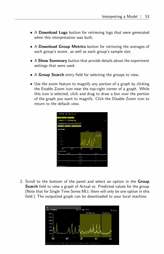
Interpreting a Model | 53

• A Download Logs button for retrieving logs that were generatedwhen this interpretation was built.

• A Download Group Metrics button for retrieving the averages ofeach group’s scorer, as well as each group’s sample size.

• A Show Summary button that provide details about the experimentsettings that were used.

• A Group Search entry field for selecting the groups to view.

• Use the zoom feature to magnify any portion of a graph by clickingthe Enable Zoom icon near the top-right corner of a graph. Whilethis icon is selected, click and drag to draw a box over the portionof the graph you want to magnify. Click the Disable Zoom icon toreturn to the default view.

2. Scroll to the bottom of the panel and select an option in the GroupSearch field to view a graph of Actual vs. Predicted values for the group.(Note that for Single Time Series MLI, there will only be one option in thisfield.) The outputted graph can be downloaded to your local machine.

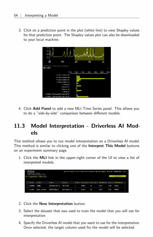
54 | Interpreting a Model

3. Click on a prediction point in the plot (white line) to view Shapley valuesfor that prediction point. The Shapley values plot can also be downloadedto your local machine.

4. Click Add Panel to add a new MLI Time Series panel. This allows youto do a ”side-by-side” comparison between different models.

11.3 Model Interpretation - Driverless AI Mod-els

This method allows you to run model interpretation on a Driverless AI model.This method is similar to clicking one of the Interpret This Model buttonson an experiment summary page.

1. Click the MLI link in the upper-right corner of the UI to view a list ofinterpreted models.

2. Click the New Interpretation button.

3. Select the dataset that was used to train the model that you will use forinterpretation.

4. Specify the Driverless AI model that you want to use for the interpretation.Once selected, the target column used fro the model will be selected.

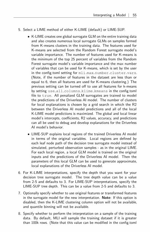
Interpreting a Model | 55

5. Select a LIME method of either K-LIME (default) or LIME-SUP.

• K-LIME creates one global surrogate GLM on the entire training dataand also creates numerous local surrogate GLMs on samples formedfrom K-means clusters in the training data. The features used forK-means are selected from the Random Forest surrogate model’svariable importance. The number of features used for K-means isthe minimum of the top 25 percent of variables from the RandomForest surrogate model’s variable importance and the max numberof variables that can be used for K-means, which is set by the userin the config.toml setting for mli max number cluster vars.(Note, if the number of features in the dataset are less than orequal to 6, then all features are used for K-means clustering.) Theprevious setting can be turned off to use all features for k-meansby setting use all columns klime kmeans in the config.tomlfile to true. All penalized GLM surrogates are trained to modelthe predictions of the Driverless AI model. The number of clustersfor local explanations is chosen by a grid search in which the R2between the Driverless AI model predictions and all of the localK-LIME model predictions is maximized. The global and local linearmodel’s intercepts, coefficients, R2 values, accuracy, and predictionscan all be used to debug and develop explanations for the DriverlessAI model’s behavior.

• LIME-SUP explains local regions of the trained Driverless AI modelin terms of the original variables. Local regions are defined byeach leaf node path of the decision tree surrogate model instead ofsimulated, perturbed observation samples - as in the original LIME.For each local region, a local GLM model is trained on the originalinputs and the predictions of the Driverless AI model. Then theparameters of this local GLM can be used to generate approximate,local explanations of the Driverless AI model.

6. For K-LIME interpretations, specify the depth that you want for yourdecision tree surrogate model. The tree depth value can be a valuefrom 2-5 and defaults to 3. For LIME-SUP interpretations, specify theLIME-SUP tree depth. This can be a value from 2-5 and defaults to 3.

7. Optionally specify whether to use original features or transformed featuresin the surrogate model for the new interpretation. Note: If this option isdisabled, then the K-LIME clustering column option will not be available,and quantile binning will not be available.

8. Specify whether to perform the interpretation on a sample of the trainingdata. By default, MLI will sample the training dataset if it is greaterthan 100k rows. (Note that this value can be modified in the config.toml

56 | Interpreting a Model

setting for mli sample size.) Turn this toggle off to run MLI on theentire dataset.

9. Optionally specify weight and dropped columns.

10. For K-LIME interpretations, optionally specify a clustering column. Notethat this column should be categorical. Also note that this is only availablewhen K-LIME is used as the LIME method and when Use OriginalFeatures is enabled. If the LIME method is changed to LIME-SUP, thenthis option is no longer available.

11. Optionally specify the number of surrogate cross-validation folds to use(from 0 to 10). When running experiments, Driverless AI automaticallysplits the training data and uses the validation data to determine theperformance of the model parameter tuning and feature engineering steps.For a new interpretation, Driverless AI uses 3 cross-validation folds bydefault for the interpretation.

12. For K-LIME interpretations, optionally specify one or more columns togenerate decile bins (uniform distribution) to help with MLI accuracy.Columns selected are added to top n columns for quantile binning selection.If a column is not numeric or not in the dataset (transformed features),then the column will be skipped. Note: This option is only availablewhen Use Original Features is enabled.

13. For K-LIME interpretations, optionally specify the number of top variableimportance numeric columns to run decile binning to help with MLIaccuracy. (Note that variable importances are generated from a RandomForest model.) This defaults to 0, and the maximum value is 10. Note:This option is only available when Use Original Features is enabled.

14. Click the Launch MLI button.

Interpreting a Model | 57

11.4 Model Interpretation - External Models

Model Interpretation does not need to be run on a Driverless AI experiment. Youcan train an external model and run Model Interpretability on the predictions.

1. Click the MLI link in the upper-right corner of the UI to view a list ofinterpreted models.

2. Click the New Interpretation button.

3. Select the dataset that you want to use for the model interpretation. Thismust include a prediction column that was generated by the externalmodel. If the dataset does not have predictions, then you can join theexternal predictions. An example showing how to do this using Python isavailable in the Driverless AI User Guide.

Note: When running interpretations on an external model, leave theSelect Model option empty. That option is for selecting a Driverless AImodel.

4. Specify a Target Column (actuals) and the Prediction Column (scoresfrom the model).

5. Select a LIME method of either K-LIME (default) or LIME-SUP.

• K-LIME creates one global surrogate GLM on the entire training dataand also creates numerous local surrogate GLMs on samples formedfrom K-means clusters in the training data. The features used forK-means are selected from the Random Forest surrogate model’svariable importance. The number of features used for K-means isthe minimum of the top 25 percent of variables from the RandomForest surrogate model’s variable importance and the max numberof variables that can be used for K-means, which is set by the userin the config.toml setting for mli max number cluster vars.(Note, if the number of features in the dataset are less than orequal to 6, then all features are used for K-means clustering.) Theprevious setting can be turned off to use all features for k-meansby setting use all columns klime kmeans in the config.tomlfile to true. All penalized GLM surrogates are trained to modelthe predictions of the Driverless AI model. The number of clusters

58 | Interpreting a Model

for local explanations is chosen by a grid search in which the R2between the Driverless AI model predictions and all of the localK-LIME model predictions is maximized. The global and local linearmodel’s intercepts, coefficients, R2 values, accuracy, and predictionscan all be used to debug and develop explanations for the DriverlessAI model’s behavior.

• LIME-SUP explains local regions of the trained Driverless AI modelin terms of the original variables. Local regions are defined byeach leaf node path of the decision tree surrogate model instead ofsimulated, perturbed observation samples - as in the original LIME.For each local region, a local GLM model is trained on the originalinputs and the predictions of the Driverless AI model. Then theparameters of this local GLM can be used to generate approximate,local explanations of the Driverless AI model.

6. For K-LIME interpretations, specify the depth that you want for yourdecision tree surrogate model. The tree depth value can be a valuefrom 2-5 and defaults to 3. For LIME-SUP interpretations, specify theLIME-SUP tree depth. This can be a value from 2-5 and defaults to 3.

7. Specify whether to perform the interpretation on a sample of the trainingdata. By default, MLI will sample the training dataset if it is greaterthan 100k rows. (Note that this value can be modified in the config.tomlsetting for mli sample size.) Turn this toggle off to run MLI on theentire dataset.

8. Optionally specify weight and dropped columns.

9. For K-LIME interpretations, optionally specify a clustering column. Alsonote that this is only available when K-LIME is used as the LIME method.If the LIME method is changed to LIME-SUP, then this option is nolonger available.

10. Optionally specify the number of surrogate cross-validation folds to use(from 0 to 10). When running experiments, Driverless AI automaticallysplits the training data and uses the validation data to determine theperformance of the model parameter tuning and feature engineering steps.For a new interpretation, Driverless AI uses 3 cross-validation folds bydefault for the interpretation.

11. For K-LIME interpretations, optionally specify one or more columns togenerate decile bins (uniform distribution) to help with MLI accuracy.Columns selected are added to top n columns for quantile binning selection.If a column is not numeric or not in the dataset (transformed features),then the column will be skipped.

Interpreting a Model | 59

12. For K-LIME interpretations, optionally specify the number of top variableimportance numeric columns to run decile binning to help with MLIaccuracy. (Note that variable importances are generated from a RandomForest model.) This value is combined with any specific columns selectedfor quantile binning. This defaults to 0, and the maximum value is 10.

13. Click the Launch MLI button.

11.5 Understanding the Model Interpretation Page

The Model Interpretation page opens with a Summary of the interpretation.This page also provides left-hand navigation for viewing additional plots. Thisnavigation includes:

• Summary: Provides a summary of the MLI experiment. See the SummaryPage section for more information.

• DAI Model: See DAI Model Dropdown for more information.

– For binary classification and regression experiments, the DAI Modelmenu provides Feature Importance and Shapley plots for transformedfeatures; a Partial Dependence and ICE plot, Disparate Impact Analy-sis plot, and Sensitivity Analysis charts, NLP Tokens and NLP LOCOfor text experiments; and Permutation Feature Importance plots forexperiments started with autodoc include permutation feature importanceenabled.

– For multiclass classification experiments, the DAI Model menu pro-vides Feature Importance and Shapley plots for transformed features.

– Note: Shapley plots are not supported for RuleFit and TensorFlowmodels. Shapley plots are also not supported for BYOR models thatDO NOT implement the has pred contribs method and DOimplement pred contribs=True in predict.

60 | Interpreting a Model

• Surrogate Models: See Surrogate Models Dropdown for more informa-tion.

– For binary classification and regression experiments, the SurrogateModel menu provides KLIME and Decision Tree plots. This alsoincludes a Random Forest submenu, which includes Global andLocal Feature Importance plots for original features and a PartialDependence plot.

– For multiclass classification experiments, the Surrogate Model menuprovides a Random Forest submenu that includes a Global FeatureImportance plot for the Random Forest surrogate model.

• Dashboard: See the Dashboard Page section for more information.

– For binary classification and regression experiments, the Dashboardpage provides a single page with a Global Interpretable Model Expla-nations plot, a Feature Importance plot, a Decision Tree plot, and aPartial Dependence plot.

– The Dashboard page is not available for multinomial experiments.

• MLI Docs: A link to the Interpreting a Model section in the online help.

• Download MLI Logs: Downloads a zip file of the logs that were gener-ated during this interpretation.

• Experiment: Provides a link back to the experiment that generated thisinterpretation.

• Scoring Pipeline:

– For binomial experiments, Scoring Pipeline option downloads thescoring pipeline for this interpretation.

– The Scoring Pipeline option is not available for multinomial experi-ments.

• Download Reason Codes:

– For binomial experiments, download a CSV file of LIME and/orShapley reason codes.

– For multinomial experiments, download a CSV file of the Shapleyreason codes.

Interpreting a Model | 61

11.5.1 Summary Page

The Summary page is the first page that opens when you view an interpretation.This page provides an overview of the interpretation, including the dataset andDriverless AI experiment (if available) that were used for the interpretationalong with the feature space (original or transformed), target column, problemtype, and k-Lime information. If the interpretation was created from a DriverlessAI model, then a table with the Driverless AI model summary is also includedalong with the top variables for the model.

11.5.2 DAI Model Dropdown

This menu provides a Feature Importance plot and a Shapley plot (not supportedfor RuleFit and TensorFlow models) for transformed features as well as PartialDependence/ICE, Disparate Impact Analysis (DIA), Sensitivity Analysis, NLPTokens and NLP LOCO (for text experiments), and Permutation Feature Impor-tance (if the autodoc include permutation feature importanceconfiguration option is enabled) plots for Driverless AI models.

Feature Importance

This plot is available for all models for binary classification, multiclass classifica-tion, and regression experiments.

This plot shows the Driverless AI feature importance. Driverless AI featureimportance is a measure of the contribution of an input variable to the overallpredictions of the Driverless AI model. Global feature importance is calculated

62 | Interpreting a Model

by aggregating the improvement in splitting criterion caused by a single variableacross all of the decision trees in the Driverless AI model.

Shapley Plot

This plot is not available for RuleFit or TensorFlow models. For all othermodels, this plot is available for binary classification, multiclass classification,and regression experiments.

Shapley explanations are a technique with credible theoretical support thatpresents consistent global and local variable contributions. Local numericShapley values are calculated by tracing single rows of data through a trainedtree ensemble and aggregating the contribution of each input variable as therow of data moves through the trained ensemble. For regression tasks, Shapleyvalues sum to the prediction of the Driverless AI model. For classificationproblems, Shapely values sum to the prediction of the Driverless AI modelbefore applying the link function. Global Shapley values are the average of theabsolute Shapley values over every row of a data set.

More information is available at https://arxiv.org/abs/1706.06060.

You can view a Shapley explanations plot by selecting the Interpret this Modelon Transformed Features button in an experiment.

Interpreting a Model | 63

Partial Dependence and Individual Conditional Expectation (ICE)

Partial dependence is a measure of the average model prediction with respectto an input variable. Partial dependence plots display how machine-learnedresponse functions change based on the values of an input variable of interest,while taking nonlinearity into consideration and averaging out the effects of allother input variables. Partial dependence plots are well-known and described inthe Elements of Statistical Learning (Hastie et all, 2001 [4]). Partial dependenceplots enable increased transparency in Driverless AI models and the ability tovalidate and debug Driverless AI models by comparing a variable’s averagepredictions across its domain to known standards, domain knowledge, andreasonable expectations. The partial dependence plot is available for binaryclassification and regression models.

Individual conditional expectation (ICE) plots, a newer and less well-knownadaptation of partial dependence plots, can be used to create more localizedexplanations for a single individual using the same basic ideas as partial de-pendence plots. ICE Plots were described by Goldstein et al (2015 [5]). ICEvalues are simply disaggregated partial dependence, but ICE is also a type ofnonlinear sensitivity analysis in which the model predictions for a single roware measured while a variable of interest is varied over its domain. ICE plotsenable a user to determine whether the model’s treatment of an individual rowof data is outside one standard deviation from the average model behavior,whether the treatment of a specific row is valid in comparison to average modelbehavior, known standards, domain knowledge, and reasonable expectations,and how a model will behave in hypothetical situations where one variable in aselected row is varied across its domain. The ICE plot is available for binaryclassification and regression models.

Given the row of input data with its corresponding Driverless AI and K -LIMEpredictions:

64 | Interpreting a Model

Taking the Driverless AI model as F(X), assuming credit scores vary from 500to 800 in the training data, and that increments of 30 are used to plot the ICEcurve, ICE is calculated as follows:

ICEcredit score,500 = F (30, 500, 1000)

ICEcredit score,530 = F (30, 530, 1000)

ICEcredit score,560 = F (30, 560, 1000)

...

ICEcredit score,800 = F (30, 800, 1000)

The one-dimensional partial dependence plots displayed here do not take inter-actions into account. Large differences in partial dependence and ICE are anindication that strong variable interactions may be present. In this case partialdependence plots may be misleading because average model behavior may notaccurately reflect local behavior.

Overlaying ICE plots onto partial dependence plots allow the comparison ofthe Driverless AI model’s treatment of certain examples or individuals to themodel’s average predictions over the domain of an input variable of interest.

This plot shows the partial dependence when a variable is selected and the ICEvalues when a specific row is selected. Users may select a point on the graphto see the specific value at that point. Partial dependence (yellow) portrays theaverage prediction behavior of the Driverless AI model across the domain of aninput variable along with +/- 1 standard deviation bands. ICE (grey) displaysthe prediction behavior for an individual row of data when an input variableis toggled across its domain. Currently, partial dependence and ICE is onlyavailable for the top ten most important original input variables. Categoricalvariables with 20 or more unique values are never included in these plots.

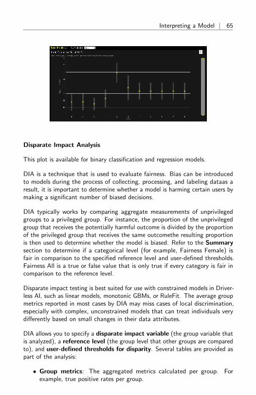
Interpreting a Model | 65

Disparate Impact Analysis

This plot is available for binary classification and regression models.

DIA is a technique that is used to evaluate fairness. Bias can be introducedto models during the process of collecting, processing, and labeling dataas aresult, it is important to determine whether a model is harming certain users bymaking a significant number of biased decisions.

DIA typically works by comparing aggregate measurements of unprivilegedgroups to a privileged group. For instance, the proportion of the unprivilegedgroup that receives the potentially harmful outcome is divided by the proportionof the privileged group that receives the same outcomethe resulting proportionis then used to determine whether the model is biased. Refer to the Summarysection to determine if a categorical level (for example, Fairness Female) isfair in comparison to the specified reference level and user-defined thresholds.Fairness All is a true or false value that is only true if every category is fair incomparison to the reference level.

Disparate impact testing is best suited for use with constrained models in Driver-less AI, such as linear models, monotonic GBMs, or RuleFit. The average groupmetrics reported in most cases by DIA may miss cases of local discrimination,especially with complex, unconstrained models that can treat individuals verydifferently based on small changes in their data attributes.

DIA allows you to specify a disparate impact variable (the group variable thatis analyzed), a reference level (the group level that other groups are comparedto), and user-defined thresholds for disparity. Several tables are provided aspart of the analysis:

• Group metrics: The aggregated metrics calculated per group. Forexample, true positive rates per group.

66 | Interpreting a Model

• Group disparity: This is calculated by dividing the metric for group bythe reference group metric. Disparity is observed if this value falls outsideof the user-defined thresholds.

• Group parity: This builds on Group disparity by converting the abovecalculation to a true or false value by applying the user-defined thresholdsto the disparity values.

In accordance with the established four-fifths rule, user-defined thresholds are setto 0.8 and 1.25 by default. These thresholds will generally detect if the model is(on average) treating the non-reference group 20% more or less favorably thanthe reference group. Users are encouraged to set the user-defined thresholds toalign with their organization’s guidance on fairness thresholds.

Notes:

• Although the process of DIA is the same for both classification and re-gression experiments, the returned information is dependent on the typeof experiment being interpreted. An analysis of a regression experimentreturns an actual vs. predicted plot, while an analysis of a binary clas-sification experiment returns confusion matrices. The above tables areprovided for both types of experiments.

• Users are encouraged to consider the explanation dashboard to understandand augment results from disparate impact analysis. In addition to itsestablished use as a fairness tool, users may want to consider disparateimpact for broader model debugging purposes. For example, users cananalyze the supplied confusion matrices and group metrics for important,non-demographic features in the Driverless AI model.

Classification Experiment

Interpreting a Model | 67

Regression Experiment

Sensitivity Analysis

Note: Sensitivity Analysis (SA) is not available for multiclass experiments.

Sensitivity Analysis (or ”What if?”) is a simple and powerful model debugging,explanation, fairness, and security tool. The idea behind SA is both directand simple: Score your trained model on a single row, on multiple rows, or onan entire dataset of potentially interesting simulated values and compare themodels new outcome to the predicted outcome on the original data.

Beyond traditional assessment practices, sensitivity analysis of machine learningmodel predictions is perhaps the most important validation technique for machinelearning models. Sensitivity analysis investigates whether model behavior andoutputs remain stable when data is intentionally perturbed or other changes aresimulated in the data. Machine learning models can make drastically differingpredictions for only minor changes in input variable values. For example, whenlooking at predictions that determine financial decisions, SA can be used tohelp you understand the impact of changing the most important input variablesand the impact of changing socially sensitive variables (such as Sex, Age, Race,etc.) in the model. If the model changes in reasonable and expected ways whenimportant variable values are changed, this can enhance trust in the model.Similarly, if the model changes to sensitive variables have minimal impact onthe model, then this is an indication of fairness in the model predictions.

This page utilizes the What If Tool for displaying the SA information.

The top portion of this page includes:

• A summary of the experiment

68 | Interpreting a Model

• Predictions for a specified column. Change the column on the Y axis toview predictions for that column.

• The current working score set. This updates each time you rescore.

The bottom portion of this page includes:

• A filter tool for filtering the analysis. Choose a different column, pre-dictions, or residuals. Set the filter type, then choose to filter by FalsePositive, False Negative, True Positive, or True Negative.

• Scoring chart. Click the Rescore button after applying a filter to updatethe scoring chart. This chart also allows you to add or remove variables,toggle the main chart aggregation, reset the data, and delete the globalhistory while resetting the data.

• The current history of actions taken on this page. You can delete individualactions by selecting the action and then clicking the Delete button thatappears.

Use Case 1: Using SA on a Single Row or on a Small Group of Rows

This section describes scenarios for using SA for explanation, debugging, security,or fairness when scoring a trained model on a single row or on a small group ofrows.

• Explanation: Change values for a variable, and then rescore the model.View the difference between the original prediction and the new model

Interpreting a Model | 69

prediction. If the change is big, then the changed variable is locallyimportant.

• Debugging: Change values for a variable, and then rescore the model.View the difference between the original prediction and the new modelprediction and determine whether the change to variable made the modelmore or less accurate.

• Security: Change values for a variable, and then rescore the model.View the difference between the original prediction and the new modelprediction. If the change is big, then the user can, for example, informtheir IT department that this variable can be used in an adversarial attackor inform the model makers that this variable should be more regularized.

• Fairness: Change values for a demographic variable, and then rescorethe model. View the difference between the original prediction and thenew model prediction. If change is big, then the user can consider usinga different model, regularizing the model more, or applying post-hoc biasremediation techniques.

• Random: Set variables to random values, and then rescore the model.This can help you look for things the you might not have thought of.

Use Case 2: Using SA on an Entire Dataset and Trained Model

This section describes scenarios for using SA for explanation, debugging, security,or fairness when scoring a trained model for an entire dataset and trainedpredictive model.

• Financial Stress Testing: Assume the user wants to see how their loandefault rates will change (according to their trained probability of defaultmodel) when they change an entire dataset to simulate that all theircustomers are under more financial stress (such as lower FICO scores,lower savings balances, higher unemployment, etc). Change the values ofthe variables in their entire dataset, and look at the Percentage Changein the average model score (default probability) on the original and newdata. They can then use this discovered information along with externalinformation and processes to understand whether their institution hasenough cash on hand to be prepared for the simulated crisis.

• Random: Set variables to random values, and then rescore the model.This allows the user to look for things the user might not have thoughtof.

Additional Resources

Sensitivity Analysis on a Driverless AI Model: This ipynb uses the UCI creditcard default data to perform sensitivity analysis and test model performance.

70 | Interpreting a Model

NLP Tokens

This plot is available for natural language processing (NLP) models.

This plot shows both the global and local importance values of each token ina corpus (a large and structured set of texts). The corpus is automaticallygenerated from text features used by Driverless AI models prior to the processof tokenization.

Local importance values are calculated by using the term frequencyinversedocument frequency (TFIDF) as a weighting factor for each token in each row.The TFIDF increases proportionally to the number of times a token appearsin a given document and is offset by the number of documents in the corpusthat contain the token. Specify the row that you want to view, then click theSearch button to see the local importance of each token in that row.

Global importance values are calculated by using the inverse document frequency(IDF), which measures how common or rare a given token is across all documents.(Default View)

Notes:

• MLI support for NLP is not available for multinomial experiments.

• MLI for NLP does not currently feature the option to remove stop words.

• By default, up to 10,000 tokens are created during the tokenizationprocess. This value can be changed in the configuration.

• By default, Driverless AI uses up to 10,000 documents to extract tokensfrom. This value can be changed with the config.mli nlp sample limitparameter. Downsampling is used for datasets that are larger than thedefault sample limit.

• Driverless AI does not currently generate a K-LIME scoring pipeline forMLI NLP problems.

Interpreting a Model | 71

NLP LOCO

This plot is available for natural language processing (NLP) models.

This plot applies a leave-one-covariate-out (LOCO) styled approach to NLPmodels by removing a specific token from all text features in a record andpredicting local importance without that token. The difference between theresulting score and the original score (token included) is useful when trying todetermine how specific changes to text features alter the predictions made bythe model.

Notes:

• MLI support for NLP is not available for multinomial experiments.

• Due to computational complexity, the global importance value is onlycalculated for :math:‘N‘ (20 by default) tokens. This value can be changedwith the mli nlp top n configuration option.

• A specific token selection method can be used by specifying one ofthe following options for the mli nlp min token mode configurationoption:

1. linspace: Selects N evenly spaced tokens according to their IDFscore (Default)

2. top: Selects top N tokens by IDF score

3. bottom: Selects bottom N tokens by IDF score

• Local values for NLP LOCO can take a significant amount of time tocalculate depending on the specifications of your hardware.

72 | Interpreting a Model

• Driverless AI does not currently generate a K-LIME scoring pipeline forMLI NLP problems.

Permutation Feature Importance

Note: The Permutation-based feature importance plot is only available if theautodoc include permutation feature importance configurationoption was enabled when starting Driverless AI or when starting the experiment.In addition, this plot is only available for binary classification and regressionexperiments.

Permutation-based feature importance shows how much a model’s performancewould change if a feature’s values were permuted. If the feature has littlepredictive power, shuffling its values should have little impact on the model’sperformance. If a feature is highly predictive, however, shuffling its valuesshould decrease the model’s performance. The difference between the model’sperformance before and after permuting the feature provides the feature’sabsolute permutation importance.

Interpreting a Model | 73

Surrogate Models Dropdown

The Surrogate Models dropdown includes K-LIME/LIME-SUP and DecisionTree plots as well as a Random Forest submenu, which includes Global andLocal Feature Importance plots for original features and a Partial Dependenceplot.

K-LIME and LIME-SUP

The MLI screen includes a K-LIME or LIME-SUP graph. A K-LIME graphis available by default when you interpret a model from the experiment page.When you create a new interpretation, you can instead choose to use LIME-SUPas the LIME method. Note that these graphs are essentially the same, but theK-LIME/LIME-SUP distinction provides insight into the LIME method that wasused during model interpretation.

The K-LIME Technique

This plot is available for binary classification and regression models.

K -LIME is a variant of the LIME technique proposed by Ribeiro at al [12].K -LIME generates global and local explanations that increase the transparencyof the Driverless AI model, and allow model behavior to be validated anddebugged by analyzing the provided plots, and comparing global and localexplanations to one-another, to known standards, to domain knowledge, and toreasonable expectations.

K-LIME creates one global surrogate GLM on the entire training data andalso creates numerous local surrogate GLMs on samples formed from K-meansclusters in the training data. The features used for K-means are selected fromthe Random Forest surrogate model’s variable importance. The number offeatures used for K-means is the minimum of the top 25 percent of variables

74 | Interpreting a Model

from the Random Forest surrogate model’s variable importance and the maxnumber of variables that can be used for K-means, which is set by the user inthe config.toml setting for mli max number cluster vars. (Note, if thenumber of features in the dataset are less than or equal to 6, then all featuresare used for K-means clustering.) The previous setting can be turned off to useall features for k-means by setting use all columns klime kmeans in theconfig.toml file to true. All penalized GLM surrogates are trained to modelthe predictions of the Driverless AI model. The number of clusters for localexplanations is chosen by a grid search in which the R2 between the DriverlessAI model predictions and all of the local K-LIME model predictions is maximized.The global and local linear model’s intercepts, coefficients, R2 values, accuracy,and predictions can all be used to debug and develop explanations for theDriverless AI model’s behavior.

LIME-SUP explains local regions of the trained Driverless AI model in termsof the original variables. Local regions are defined by each leaf node path ofthe decision tree surrogate model instead of simulated, perturbed observationsamples - as in the original LIME. For each local region, a local GLM model istrained on the original inputs and the predictions of the Driverless AI model.Then the parameters of this local GLM can be used to generate approximate,local explanations of the Driverless AI model.

The parameters of the global K -LIME model give an indication of overall linearfeature importance and the overall average direction in which an input variableinfluences the Driverless AI model predictions. The global model is also usedto generate explanations for very small clusters (N < 20) where fitting a locallinear model is inappropriate.

The in-cluster linear model parameters can be used to profile the local region,to give an average description of the important variables in the local region,and to understand the average direction in which an input variable affects theDriverless AI model predictions. For a point within a cluster, the sum of the locallinear model intercept and the products of each coefficient with their respectiveinput variable value are the K -LIME prediction. By disaggregating the K -LIMEpredictions into individual coefficient and input variable value products, thelocal linear impact of the variable can be determined. This product is sometimesreferred to as a reason code and is used to create explanations for the DriverlessAI model’s behavior.

In the following example, reason codes are created by evaluating and disaggre-gating a local linear model.

Given the row of input data with its corresponding Driverless AI and K -LIMEpredictions:

Interpreting a Model | 75

And the local linear model:

yK -LIME = 0.1 + 0.01 ∗ debt to income ratio + 0.0005 ∗ credit score + 0.0002 ∗ savings account balance

It can be seen that the local linear contributions for each variable are:

• debt to income ratio: 0.01 * 30 = 0.3

• credit score: 0.0005 * 600 = 0.3

• savings acct balance: 0.0002 * 1000 = 0.2

Each local contribution is positive and thus contributes positively to the Driver-less AI model’s prediction of 0.85 for H2OAI predicted default. By taking intoconsideration the value of each contribution, reason codes for the Driverless AIdecision can be derived. debt to income ratio and credit score would be thetwo largest negative reason codes, followed by savings acct balance.

The local linear model intercept and the products of each coefficient andcorresponding value sum to the K -LIME prediction. Moreover it can be seenthat these linear explanations are reasonably representative of the nonlinearmodel’s behavior for this individual because the K -LIME predictions are within5.5% of the Driverless AI model prediction. This information is encoded intoEnglish language rules which can be viewed by clicking the Explanations button.

Like all LIME explanations based on linear models, the local explanations arelinear in nature and are offsets from the baseline prediction, or intercept, whichrepresents the average of the penalized linear model residuals. Of course, linearapproximations to complex non-linear response functions will not always createsuitable explanations and users are urged to check the K -LIME plot, the localmodel R2, and the accuracy of the K -LIME prediction to understand the validityof the K -LIME local explanations. When K -LIME accuracy for a given pointor set of points is quite low, this can be an indication of extremely nonlinearbehavior or the presence of strong or high-degree interactions in this local regionof the Driverless AI response function. In cases where K -LIME linear modelsare not fitting the Driverless AI model well, nonlinear LOCO feature importancevalues may be a better explanatory tool for local model behavior. As K -LIMElocal explanations rely on the creation of k-means clusters, extremely wide inputdata or strong correlation between input variables may also degrade the qualityof K -LIME local explanations.

The LIME-SUP Technique

76 | Interpreting a Model

This plot is available for binary classification and regression models.

LIME-SUP explains local regions of the trained Driverless AI model in termsof the original variables. Local regions are defined by each leaf node path ofthe decision tree surrogate model instead of simulated, perturbed observationsamples - as in the original LIME. For each local region, a local GLM model istrained on the original inputs and the predictions of the Driverless AI model.Then the parameters of this local GLM can be used to generate approximate,local explanations of the Driverless AI model.

The Global Interpretable Model Explanation Plot

This plot shows Driverless AI model predictions and LIME model predictionsin sorted order by the Driverless AI model predictions. This graph is interac-tive. Hover over the Model Prediction, LIME Model Prediction, or ActualTarget radio buttons to magnify the selected predictions. Or click those radiobuttons to disable the view in the graph. You can also hover over any point inthe graph to view LIME reason codes for that value. By default, this plot showsinformation for the global LIME model, but you can change the plot view toshow local results from a specific cluster. The LIME plot also provides a visualindication of the linearity of the Driverless AI model and the trustworthinessof the LIME explanations. The closer the local linear model approximates theDriverless AI model predictions, the more linear the Driverless AI model andthe more accurate the explanation generated by the LIME local linear models.

Decision Tree

The decision tree surrogate model increases the transparency of the DriverlessAI model by displaying an approximate flowchart of the complex DriverlessAI model’s decision making process. The decision tree surrogate model alsodisplays the most important variables in the Driverless AI model and the mostimportant interactions in the Driverless AI model. The decision tree surrogatemodel can be used for visualizing, validating, and debugging the Driverless AI

Interpreting a Model | 77

model by comparing the displayed decision-process, important variables, andimportant interactions to known standards, domain knowledge, and reasonableexpectations.

A surrogate model is a data mining and engineering technique in which agenerally simpler model is used to explain another, usually more complex, modelor phenomenon. The decision tree surrogate is known to date back at leastto 1996 (Craven and Shavlik, [2]). The decision tree surrogate model hereis trained to predict the predictions of the more complex Driverless AI modelusing the of original model inputs. The trained surrogate model enables aheuristic understanding (i.e., not a mathematically precise understanding) ofthe mechanisms of the highly complex and nonlinear Driverless AI model.

In the decision tree plot, the highlighted row shows the path to the highestprobability leaf node and indicates the globally important variables and inter-actions that influence the Driverless AI model prediction for that row. Thedecision tree plot is available for binary classification and regression models.

11.5.3 Random Forest Dropdown

The Random Forest dropdown provides a submenu that includes a FeatureImportance plot, a Partial Dependence plot, and a LOCO plot. These plots arefor original features rather than transformed features.

Global Feature Importance vs Local Feature Importance

Global feature importance (yellow) is a measure of the contribution of an inputvariable to the overall predictions of the Driverless AI model. Global featureimportance is calculated by aggregating the improvement in splitting criterioncaused by a single variable across all of the decision trees in the Driverless AImodel. Local feature importance (grey) is a measure of the contribution of aninput variable to a single prediction of the Driverless AI model. Local featureimportance is calculated by removing the contribution of a variable from everydecision tree in the Driverless AI model and measuring the difference betweenthe prediction with and without the variable. Both global and local variableimportance are scaled so that the largest contributor has a value of 1.

78 | Interpreting a Model

Note: Engineered features are used for MLI when a time series experiment isbuilt. This is because munged time series features are more useful features forMLI compared to raw time series features.

LOCO

Local feature importance describes how the combination of the learned modelrules or parameters and an individual row’s attributes affect a model’s predictionfor that row while taking nonlinearity and interactions into effect. Local featureimportance values reported here are based on a variant of the leave-one-covariate-out (LOCO) method (Lei et al, 2017 [9]).

In the LOCO-variant method, each local feature importance is found by re-scoring the trained Driverless AI model for each feature in the row of interest,while removing the contribution to the model prediction of splitting rules thatcontain that feature throughout the ensemble. The original prediction is thensubtracted from this modified prediction to find the raw, signed importancefor the feature. All local feature importance values for the row are then scaledbetween 0 and 1 for direct comparison with global feature importance values.

Given the row of input data with its corresponding Driverless AI and K -LIMEpredictions:

Taking the Driverless AI model as F(X), LOCO-variant feature importancevalues are calculated as follows.

First, the modified predictions are calculated:

F debt to income ratio = F (NA, 600, 1000) = 0.99

Interpreting a Model | 79

F credit score = F (30, NA, 1000) = 0.73

F savings acct balance = F (30, 600, NA) = 0.82

Second, the original prediction is subtracted from each modified prediction togenerate the unscaled local feature importance values:

LOCOdebt to income ratio = F debt to income ratio − 0.85 = 0.99 −0.85 = 0.14

LOCOcredit score = F credit score − 0.85 = 0.73− 0.85 = −0.12

LOCOsavings acct balance = F savings acct balance − 0.85 = 0.82 −0.85 = −0.03

Finally LOCO values are scaled between 0 and 1 by dividing each value for therow by the maximum value for the row and taking the absolute magnitude ofthis quotient.

Scaled(LOCOdebt to income ratio) = Abs(LOCO debt to income ratio/0.14) =1

Scaled(LOCOcredit score) = Abs(LOCO credit score/0.14) = 0.86

Scaled(LOCOsavings acct balance) = Abs(LOCO savings acct balance/0.14) =0.21

One drawback to these LOCO-variant feature importance values is, unlikeK -LIME, it is difficult to generate a mathematical error rate to indicate whenLOCO values may be questionable.

Partial Dependence and Individual Conditional Expectation

A Partial Dependence and ICE plot is available for both Driverless AI andsurrogate models. Refer to the previous Partial Dependence and IndividualConditional Expectation section for more information about this plot.

80 | Interpreting a Model

NLP Surrogate Models

These plots are available for natural language processing (NLP) models.

For NLP surrogate models, Driverless AI creates a TFIDF matrix by tokenizingall text features. The resulting frame is appended to numerical or categoricalcolumns from the training dataset, and the original text columns are removed.This frame is then used for training surrogate models that have predictioncolumns consisting of tokens and the original numerical or categorical features.

Notes:

• MLI support for NLP is not available for multinomial experiments.

• Each row in the TFIDF matrix contains N columns, where N is the totalnumber of tokens in the corpus with values that are appropriate for thatrow (0 if absent).

• Driverless AI does not currently generate a K-LIME scoring pipeline forMLI NLP problems.

11.5.4 Dashboard Page

The Model Interpretation Dashboard includes the following information:

• Global interpretable model explanation plot

• Feature importance (Global for original features; LOCO for interpretationswith predictions and when interpreting on raw features)

• Decision tree surrogate model

• Partial dependence and individual conditional expectation plots

Interpreting a Model | 81

11.6 General Considerations

11.6.1 Machine Learning and Approximate Explanations

For years, common sense has deemed the complex, intricate formulas created bytraining machine learning algorithms to be uninterpretable. While great advanceshave been made in recent years to make these often nonlinear, non-monotonic,and non-continuous machine-learned response functions more understandable(Hall et al, 2017 [7]), it is likely that such functions will never be as directly oruniversally interpretable as more traditional linear models.

Why consider machine learning approaches for inferential purposes? In general,linear models focus on understanding and predicting average behavior, whereasmachine-learned response functions can often make accurate, but more difficultto explain, predictions for subtler aspects of modeled phenomenon. In a sense,linear models create very exact interpretations for approximate models. Theapproach here seeks to make approximate explanations for very exact models.It is quite possible that an approximate explanation of an exact model mayhave as much, or more, value and meaning than the exact interpretations ofan approximate model. Moreover, the use of machine learning techniques forinferential or predictive purposes does not preclude using linear models forinterpretation (Ribeiro et al, 2016 [12]).

82 | Interpreting a Model

11.6.2 The Multiplicity of Good Models in Machine Learn-ing

It is well understood that for the same set of input variables and predictiontargets, complex machine learning algorithms can produce multiple accuratemodels with very similar, but not exactly the same, internal architectures(Brieman, 2001 [1]). This alone is an obstacle to interpretation, but when usingthese types of algorithms as interpretation tools or with interpretation tools it isimportant to remember that details of explanations will change across multipleaccurate models.

11.6.3 Expectations for Consistency Between ExplanatoryTechniques

• The decision tree surrogate is a global, nonlinear description of theDriverless AI model behavior. Variables that appear in the tree shouldhave a direct relationship with variables that appear in the global featureimportance plot. For certain, more linear Driverless AI models, variablesthat appear in the decision tree surrogate model may also have largecoefficients in the global K -LIME model.

• K -LIME explanations are linear, do not consider interactions, and representoffsets from the local linear model intercept. LOCO importance valuesare nonlinear, do consider interactions, and do not explicitly considera linear intercept or offset. LIME explanations and LOCO importancevalues are not expected to have a direct relationship but can align roughlyas both are measures of a variable’s local impact on a model’s predictions,especially in more linear regions of the Driverless AI model’s learnedresponse function.

• ICE is a type of nonlinear sensitivity analysis which has a complex relation-ship to LOCO feature importance values. Comparing ICE to LOCO canonly be done at the value of the selected variable that actually appearsin the selected row of the training data. When comparing ICE to LOCOthe total value of the prediction for the row, the value of the variablein the selected row, and the distance of the ICE value from the averageprediction for the selected variable at the value in the selected row mustall be considered.

• ICE curves that are outside the standard deviation of partial dependencewould be expected to fall into less populated decision paths of the decisiontree surrogate; ICE curves that lie within the standard deviation of partialdependence would be expected to belong to more common decision paths.

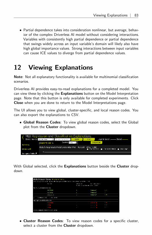
Viewing Explanations | 83

• Partial dependence takes into consideration nonlinear, but average, behav-ior of the complex Driverless AI model without considering interactions.Variables with consistently high partial dependence or partial dependencethat swings widely across an input variable’s domain will likely also havehigh global importance values. Strong interactions between input variablescan cause ICE values to diverge from partial dependence values.

12 Viewing ExplanationsNote: Not all explanatory functionality is available for multinomial classificationscenarios.

Driverless AI provides easy-to-read explanations for a completed model. Youcan view these by clicking the Explanations button on the Model Interpretationpage. Note that this button is only available for completed experiments. ClickClose when you are done to return to the Model Interpretations page.

The UI allows you to view global, cluster-specific, and local reason codes. Youcan also export the explanations to CSV.

• Global Reason Codes: To view global reason codes, select the Globalplot from the Cluster dropdown.

With Global selected, click the Explanations button beside the Cluster drop-down.

• Cluster Reason Codes: To view reason codes for a specific cluster,select a cluster from the Cluster dropdown.

84 | Viewing Explanations

With a cluster selected, click the Explanations button.

• Local Reason Codes by Row Number: To view local reason codes fora specific row, select a point on the graph or type a value in the Valuefield.

With a value selected, click the Explanations button in the upper-rightcorner.

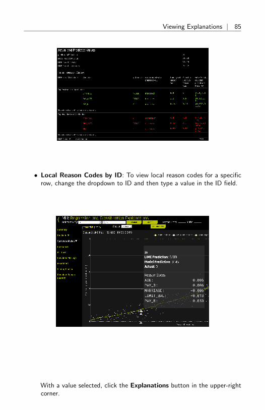
Viewing Explanations | 85

• Local Reason Codes by ID: To view local reason codes for a specificrow, change the dropdown to ID and then type a value in the ID field.

With a value selected, click the Explanations button in the upper-rightcorner.

86 | Transform Another Dataset

13 Score on Another Dataset

After you generate a model, you can use that model to make predictions onanother dataset.

1. Click the Experiments link in the top menu and select the experimentthat you want to use.

2. On the Experiments page, click the Score on Another Dataset button.

3. Locate the new dataset that you want to score on. Note that this newdataset must include the same columns as the dataset used in selectedexperiment.

4. Click Select at the top of the screen. This immediately starts the scoringprocess.

5. Click the Download Predictions button after scoring is complete.

14 Transform Another Dataset

When a training dataset is used in an experiment, Driverless AI transforms thedata into an improved, feature engineered dataset. (Refer to About DriverlessAI Transformations for more information about the transformations that areprovided in Driverless AI.) But what happens when new rows are added to yourdataset? In this case, you can specify to transform the new dataset after addingit to Driverless AI, and the same transformations that Driverless AI applied tothe original dataset will be applied to these new rows.

Follow these steps to transform another dataset. Note that this assumes thenew dataset has been added to Driverless AI already.

Transform Another Dataset | 87

Note: Transform Another Dataset is not available for Time Series experi-ments.

1. On the completed experiment page for the original dataset, click theTransform Another Dataset button.

2. Select the new training dataset that you want to transform. Note thatthis must have the same number columns as the original dataset.

3. In the Select drop down, specify a validation dataset to use with thisdataset, or specify to split the training data. If you specify to split thedata, then you also specify the split value (defaults to 25 percent) andthe seed (defaults to 1234). Note: To ensure the transformed datasetrespects the row order, choose a validation dataset instead of splittingthe training data. Splitting the training data will result in a shuffling ofthe row order.

4. Optionally specify a test dataset. If specified, then the output also includethe final test dataset for final scoring.

5. Click Launch Transformation.

The following datasets will be available for download upon successful completion:

• Training dataset (not for cross validation)

• Validation dataset for parameter tuning

• Test dataset for final scoring. This option is available if a test datasetwas used.

88 | The Driverless AI Scoring Pipelines

15 The Driverless AI Scoring Pipelines

Driverless AI provides several Scoring Pipelines for experiments and/or inter-preted models.

• A standalone Python Scoring Pipeline is available for experiments andinterpreted models.

• A low-latency, standalone MOJO Scoring Pipeline is available for experi-ments, with both Java and C++ backends.

The Python Scoring Pipeline is implemented as a Python whl file. Whilethis allows for a single process scoring engine, the scoring service is generallyimplemented as a client/server architecture and supports interfaces for TCPand HTTP.

The MOJO Scoring Pipeline provides a standalone scoring pipeline that convertsexperiments to MOJOs, which can be scored in real time. The MOJO ScoringPipeline is available as either a pure Java runtime or a C++ runtime. For theC++ runtime, both Python and R wrappers are provided.

15.1 Visualize the Scoring Pipeline

A visualization of the scoring pipeline is available for each completed experiment.Note: This pipeline is best viewed in the latest version of Chrome.

Click the Visualize Scoring Pipeline (Experimental) button on the completedexperiment page to view the visualization.

The Driverless AI Scoring Pipelines | 89

To view a visual representation of a specific model, click on the oval thatcorresponds with that model.

To change the orientation of the visualization, click the Transpose button inthe bottom right-hand corner of the screen.

90 | The Driverless AI Scoring Pipelines

15.2 Which Pipeline Should I Use?

Driverless AI provides a Python Scoring Pipeline, an MLI Standalone Scor-ing Pipeline, and a MOJO Scoring Pipeline. Consider the following whendetermining the scoring pipeline that you want to use.

• For all pipelines, the higher the accuracy, the slower the scoring.

• The Python Scoring Pipeline is slower but easier to use than the MOJOscoring pipeline.

• When running the Python Scoring Pipeline:

– HTTP is easy and is supported by virtually any language. HTTPsupports RESTful calls via curl, wget, or supported packages invarious scripting languages.

– TCP is a bit more complex, though faster. TCP also requires Thrift,which currently does not handle NAs.

• The MOJO Scoring Pipeline is flexible and is faster than the PythonScoring Pipeline, but it requires a bit more coding. The MOJO ScoringPipeline is available as either a pure Java runtime or a C++ runtime.

• The MLI Standalone Python Scoring Pipeline can be used to scoreinterpreted models but only supports k-LIME reason codes.

– For obtaining k-LIME reason codes from an MLI experiment, usethe MLI Standalone Python Scoring Pipeline. k-LIME reason codesare available for all models.

– For obtaining Shapley reason codes from an MLI experiment, use theDAI Standalone Python Scoring Pipeline. Shapley is only availablefor XGBoost and LightGBM models. Note that obtaining Shapleyreason codes through the Python Scoring Pipeline can be timeconsuming.

The Driverless AI Scoring Pipelines | 91

15.3 Driverless AI Standalone Python ScoringPipeline

As indicated earlier, a scoring pipeline is available after a successfully completedexperiment. This package contains an exported model and Python 3.6 sourcecode examples for productionizing models built using H2O Driverless AI.

The files in this package allow you to transform and score on new data in acouple of different ways:

• From Python 3.6, you can import a scoring module, and then use themodule to transform and score on new data.

• From other languages and platforms, you can use the TCP/HTTP scoringservice bundled with this package to call into the scoring pipeline modulethrough remote procedure calls (RPC).

Notes:

• Previous Python Scoring Pipeline wheel packages contain unconstrainedversions of dependencies that can break the scoring package. To avoidpotential errors, navigate to the environment that contains the scoringpackage and force the installation of upgraded versions of the outdateddependencies from the command line:

pip install --upgrade gitdb2==2.0.6 gitdb==0.6.4

• By default, if a custom recipe has been uploaded into Driverless AI but isnot used in the experiment, then the Python Scoring Pipeline still containsthe H2O recipe server. If this pipeline is then deployed in a container, theH2O recipe server causes the size of the pipeline to be much larger. Inaddition, Java has to be installed in the container, which further increasesthe runtime storage and memory requirements. A workaround is to setthe following environment variable before running the Python ScoringPipeline:

export dai_enable_custom_recipes=0

15.3.1 Python Scoring Pipeline Files

The scoring-pipeline folder includes the following notable files:

• example.py: An example Python script demonstrating how to importand score new records.

92 | The Driverless AI Scoring Pipelines

• run example.sh: Runs example.py (also sets up a virtualenv with pre-requisite libraries).

• tcp server.py: A standalone TCP server for hosting scoring services.

• http server.py: A standalone HTTP server for hosting scoring services.

• run tcp server.sh: Runs TCP scoring service (runs server.py).

• run http server.sh: Runs HTTP scoring service (runs server.py).

• example client.py: An example Python script demonstrating how tocommunicate with the scoring server.

• run tcp client.sh: Demonstrates how to communicate with the scoringservice via TCP (runs example client.py).

• run http client.sh: Demonstrates how to communicate with the scoringservice via HTTP (using curl).

15.3.2 Quick Start - Recommended Method

This is the recommended method for running the Python Scoring Pipeline. Usethis method if:

• You have an air gapped environment with no access to the Internet.

• You are running Power.

• You want an easy quick start approach.

Prerequisites

• A valid Driverless AI license key

• A completed Driverless AI experiment

• Downloaded Python Scoring Pipeline

Running the Python Scoring Pipeline - Recommended

1. On https://www.h2o.ai/download/, download the TAR SH version ofDriverless AI (for either Linux or IBM Power).

2. Use bash to execute the download. This creates a new dai-nnn folder.

3. Change directories into the new Driverless AI folder.

cd dai-nnn directory.

4. Run the following to install the Python Scoring Pipeline for your completedDriverless AI experiment:

The Driverless AI Scoring Pipelines | 93

./dai-env.sh pip install /path/to/your/scoring_experiment.whl

5. Run the following command to run the included scoring pipeline example:

DRIVERLESS_AI_LICENSE_KEY="pastekeyhere"SCORING_PIPELINE_INSTALL_DEPENDENCIES=0 ./dai-env.sh

15.3.3 Quick Start - Alternative Method

This section describes an alternative method for running the Python ScoringPipeline. This version requires Internet access. It is also not supported onPower machines.

Prerequisites

The following are required in order to run the downloaded scoring pipeline.

• The scoring module and scoring service are supported only on Linuxx86 64 with Python 3.6 and OpenBLAS.

• The scoring module and scoring service download additional packagesat install time and require Internet access. Depending on your networkenvironment, you might need to set up internet access via a proxy.

• Valid Driverless AI license. Driverless AI requires a license to be specifiedin order to run the Python Scoring Pipeline.

• Apache Thrift (to run the TCP scoring service)

• Linux x86 64 environment

• Python 3.6

• libopenblas-dev (required for H2O4GPU)

• Internet access to download and install packages. Note that dependingon your environment, you may also need to set up proxy.

• OpenCL

Examples of how to install these prerequisites are below:

Installing Python 3.6 and OpenBlas Ubuntu 16.10+

$ sudo apt install python3.6 python3.6-dev python3-pip python3-dev \python-virtualenv python3-virtualenv libopenblas-dev

Installing Python 3.6 and OpenBLAS on Ubuntu 16.4

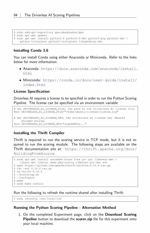
94 | The Driverless AI Scoring Pipelines

$ sudo add-apt-repository ppa:deadsnakes/ppa$ sudo apt-get update$ sudo apt-get install python3.6 python3.6-dev python3-pip python3-dev \

python-virtualenv python3-virtualenv libopenblas-dev

Installing Conda 3.6

You can install Conda using either Anaconda or Miniconda. Refer to the linksbelow for more information:

• Anaconda: https://docs.anaconda.com/anaconda/install.html

• Miniconda: https://conda.io/docs/user-guide/install/index.html

License Specification

Driverless AI requires a license to be specified in order to run the Python ScoringPipeline. The license can be specified via an environment variable:

# Set DRIVERLESS_AI_LICENSE_FILE, the path to the Driverless AI license file%env DRIVERLESS_AI_LICENSE_FILE="/home/ubuntu/license/license.sig"

# Set DRIVERLESS_AI_LICENSE_KEY, the Driverless AI license key (Base64encoded string)

%env DRIVERLESS_AI_LICENSE_KEY="oLqLZXMI0y..."

Installing the Thrift Compiler

Thrift is required to run the scoring service in TCP mode, but it is not re-quired to run the scoring module. The following steps are available on theThrift documentation site at: https://thrift.apache.org/docs/BuildingFromSource.

$ sudo apt-get install automake bison flex g++ git libevent-dev \libssl-dev libtool make pkg-config libboost-all-dev ant

$ wget https://github.com/apache/thrift/archive/0.10.0.tar.gz$ tar -xvf 0.10.0.tar.gz$ cd thrift-0.10.0$ ./bootstrap.sh$ ./configure$ make$ sudo make install

Run the following to refresh the runtime shared after installing Thrift:

$ sudo ldconfig /usr/local/lib

Running the Python Scoring Pipeline - Alternative Method

1. On the completed Experiment page, click on the Download ScoringPipeline button to download the scorer.zip file for this experiment ontoyour local machine.

The Driverless AI Scoring Pipelines | 95

2. Unzip the scoring pipeline.

After the pipeline is downloaded and unzipped, you will be able to run thescoring module and the scoring service.

Score from a Python Program

If you intend to score from a Python program, run the scoring module example.(Requires Linux x86 64 and Python 3.6.)

$ export DRIVERLESS_AI_LICENSE_FILE="/path/to/license.sig"$ bash run_example.sh

Score Using a Web Service

If you intend to score using a web service, run the HTTP scoring server example.(Requires Linux x86 64 and Python 3.6.)

$ export DRIVERLESS_AI_LICENSE_FILE="/path/to/license.sig"$ bash run_http_server.sh$ bash run_http_client.sh

Score Using a Thrift Service

If you intend to score using a Thrift service, run the TCP scoring server example.(Requires Linux x86 64, Python 3.6 and Thrift.)

$ export DRIVERLESS_AI_LICENSE_FILE="/path/to/license.sig"$ bash run_tcp_server.sh$ bash run_tcp_client.sh

Note: By default, the run *.sh scripts mentioned above create a virtualenvironment using virtualenv and pip, within which the Python code is executed.The scripts can also leverage Conda (Anaconda/Mininconda) to create Condavirtual environment and install required package dependencies. The packagemanager to use is provided as an argument to the script.

# to use conda package manager$ export DRIVERLESS_AI_LICENSE_FILE="/path/to/license.sig"$ bash run_example.sh --pm conda

# to use pip package manager$ export DRIVERLESS_AI_LICENSE_FILE="/path/to/license.sig"$ bash run_example.sh --pm pip

Note: If you experience errors while running any of the above scripts, pleasecheck to make sure your system has a properly installed and configured Python3.6 installation. Refer to the Troubleshooting Python Environment Issues sectionat the end of this chapter to see how to set up and test the scoring moduleusing a cleanroom Ubuntu 16.04 virtual machine.

96 | The Driverless AI Scoring Pipelines

15.3.4 The Python Scoring Module

The scoring module is a Python module bundled into a standalone wheel file(name scoring *.whl). All the prerequisites for the scoring module to workcorrectly are listed in the requirements.txt file. To use the scoring module, allyou have to do is create a Python virtualenv, install the prerequisites, and thenimport and use the scoring module as follows:

# See ’example.py’ for complete example.from scoring_487931_20170921174120_b4066 import Scorerscorer = Scorer() # Create instance.score = scorer.score([ # Call score()

7.416, # sepal_len3.562, # sepal_wid1.049, # petal_len2.388, # petal_wid

])

The scorer instance provides the following methods (and more):

• score(list): Score one row (list of values).

• score batch(df): Score a Pandas dataframe.

• fit transform batch(df): Transform a Pandas dataframe.

• get target labels(): Get target column labels (for classification problems).

The process of importing and using the scoring module is demonstrated by thebash script run example.sh, which effectively performs the following steps:

# See ’run_example.sh’ for complete example.$ virtualenv -p python3.6 env$ source env/bin/activate$ pip install -r requirements.txt$ export DRIVERLESS_AI_LICENSE_FILE="/path/to/license.sig"$ python example.py

15.3.5 The Scoring Service

The scoring service hosts the scoring module as an HTTP or TCP service.Doing this exposes all the functions of the scoring module through remoteprocedure calls (RPC). In effect, this mechanism allows you to invoke scoringfunctions from languages other than Python on the same computer or fromanother computer on a shared network or on the Internet.

The scoring service can be started in two ways:

• In TCP mode, the scoring service provides high-performance RPC callsvia Apache Thrift (https://thrift.apache.org/) using a binarywire protocol.

The Driverless AI Scoring Pipelines | 97

• In HTTP mode, the scoring service provides JSON-RPC 2.0 calls servedby Tornado (http://www.tornadoweb.org).

Scoring operations can be performed on individual rows (row-by-row) or inbatch mode (multiple rows at a time).

Scoring Service - TCP Mode (Thrift)

The TCP mode allows you to use the scoring service from any language supportedby Thrift, including C, C++, C#, Cocoa, D, Dart, Delphi, Go, Haxe, Java,Node.js, Lua, perl, PHP, Python, Ruby and Smalltalk.

To start the scoring service in TCP mode, you will need to generate the Thriftbindings once, then run the server:

# See ’run_tcp_server.sh’ for complete example.$ thrift --gen py scoring.thrift$ python tcp_server.py --port=9090

Note that the Thrift compiler is only required at build-time. It is not a run timedependency, i.e. once the scoring services are built and tested, you do not needto repeat this installation process on the machines where the scoring servicesare intended to be deployed.

To call the scoring service, simply generate the Thrift bindings for your languageof choice, then make RPC calls via TCP sockets using Thrift’s buffered transportin conjunction with its binary protocol.

# See ’run_tcp_client.sh’ for complete example.$ thrift --gen py scoring.thrift

# See ’example_client.py’ for complete example.socket = TSocket.TSocket(’localhost’, 9090)transport = TTransport.TBufferedTransport(socket)protocol = TBinaryProtocol.TBinaryProtocol(transport)client = ScoringService.Client(protocol)transport.open()row = Row()row.sepalLen = 7.416 # sepal_lenrow.sepalWid = 3.562 # sepal_widrow.petalLen = 1.049 # petal_lenrow.petalWid = 2.388 # petal_widscores = client.score(row)transport.close()

You can reproduce the exact same result from other languages, e.g. Java:

$ thrift --gen java scoring.thrift

// Dependencies:// commons-codec-1.9.jar// commons-logging-1.2.jar// httpclient-4.4.1.jar// httpcore-4.4.1.jar// libthrift-0.10.0.jar// slf4j-api-1.7.12.jar

98 | The Driverless AI Scoring Pipelines

import ai.h2o.scoring.Row;import ai.h2o.scoring.ScoringService;import org.apache.thrift.TException;import org.apache.thrift.protocol.TBinaryProtocol;import org.apache.thrift.transport.TSocket;import org.apache.thrift.transport.TTransport;import java.util.List;

public class Main {public static void main(String[] args) {try {TTransport transport = new TSocket("localhost", 9090);transport.open();

ScoringService.Client client = new ScoringService.Client(new TBinaryProtocol(transport));

Row row = new Row(7.642, 3.436, 6.721, 1.020);List<Double> scores = client.score(row);System.out.println(scores);

transport.close();} catch (TException ex) {ex.printStackTrace();

}}

}

Scoring Service - HTTP Mode (JSON-RPC 2.0)

The HTTP mode allows you to use the scoring service using plaintext JSON-RPC calls. This is usually less performant compared to Thrift, but has theadvantage of being usable from any HTTP client library in your language ofchoice, without any dependency on Thrift.

See http://www.jsonrpc.org/specification for JSON-RPC docu-mentation.

To start the scoring service in HTTP mode:

# See ’run_http_server.sh’ for complete example.$ export DRIVERLESS_AI_LICENSE_FILE="/path/to/license.sig"$ python http_server.py --port=9090

To invoke scoring methods, compose a JSON-RPC message and make a HTTPPOST request to http://host:port/rpc as follows:

# See ’run_http_client.sh’ for complete example.$ curl http://localhost:9090/rpc \--header "Content-Type: application/json" \--data @- <<EOF

{"id": 1,"method": "score","params": {"row": [ 7.486, 3.277, 4.755, 2.354 ]

}}

The Driverless AI Scoring Pipelines | 99

EOF

Similarly, you can use any HTTP client library to reproduce the above result.For example, from Python, you can use the requests module as follows:

import requestsrow = [7.486, 3.277, 4.755, 2.354]req = dict(id=1, method=’score’, params=dict(row=row))res = requests.post(’http://localhost:9090/rpc’, data=req)print(res.json()[’result’])

15.3.6 Python Scoring Pipeline FAQ

Why am I getting a ”TensorFlow is disabled” message when I run thePython Scoring Pipeline?

If you ran an experiment when TensorFlow was enabled and then attempt torun the Python Scoring Pipeline, you may receive a message similar to thefollowing:

TensorFlow is disabled. To enable, export DRIVERLESS_AI_ENABLE_TENSORFLOW=1or set enable_tensorflow=true in config.toml.

This can be fixed by enabling the DRIVERLESS AI ENABLE TENSORFLOWflag when running the Python Scoring Pipeline. For example:

$ export DRIVERLESS_AI_LICENSE_FILE="/path/to/license.sig"$ DRIVERLESS_AI_ENABLE_TENSORFLOW=1 bash run_example.sh

15.3.7 Troubleshooting Python Environment Issues

The following instructions describe how to set up a cleanroom Ubuntu 16.04virtual machine to test that this scoring pipeline works correctly.

Prerequisites:

• Install Virtualbox: sudo apt-get install virtualbox

• Install Vagrant: https://www.vagrantup.com/downloads.html

1. Create configuration files for Vagrant.

• bootstrap.sh: contains commands to set up Python 3.6 and Open-BLAS.

• Vagrantfile: contains virtual machine configuration instructions forVagrant and VirtualBox.

100 | The Driverless AI Scoring Pipelines

----- bootstrap.sh -----

#!/usr/bin/env bash

sudo apt-get -y updatesudo apt-get -y install apt-utils build-essential python-software-

properties software-properties-common zip libopenblas-devsudo add-apt-repository -y ppa:deadsnakes/ppasudo apt-get update -yqqsudo apt-get install -y python3.6 python3.6-dev python3-pip python3-dev

python-virtualenv python3-virtualenv

# end of bootstrap.sh

----- Vagrantfile -----

# -*- mode: ruby -*-# vi: set ft=ruby :

Vagrant.configure(2) do |config|config.vm.box = "ubuntu/xenial64"config.vm.provision :shell, path: "bootstrap.sh", privileged: falseconfig.vm.hostname = "h2o"config.vm.provider "virtualbox" do |vb|vb.memory = "4096"

endend

# end of Vagrantfile

2. Launch the VM and SSH into it. Note that we are also placing the scoringpipeline in the same directory so that we can access it later inside theVM.

cp /path/to/scorer.zip .vagrant upvagrant ssh

3. Test the scoring pipeline inside the virtual machine.

cp /vagrant/scorer.zip .unzip scorer.zipcd scoring-pipeline/export DRIVERLESS_AI_LICENSE_FILE="/path/to/license.sig"bash run_example.sh

At this point, you should see scores printed out on the terminal. If not, contactus at support@h2o.ai.

15.4 Driverless AI MLI Standalone Scoring Pack-age

This package contains an exported model and Python 3.6 source code examplesfor productionizing models built using H2O Driverless AI’s Machine Learning

The Driverless AI Scoring Pipelines | 101

Interpretability (MLI) tool. This is only available for interpreted models andcan be downloaded by clicking the Scoring Pipeline button on the InterpretedModels page.

The files in this package allow you to obtain reason codes for a given row ofdata in a couple of different ways:

• From Python 3.6, you can import a scoring module, and then use themodule to transform and score on new data.

• From other languages and platforms, you can use the TCP/HTTP scoringservice bundled with this package to call into the scoring pipeline modulethrough remote procedure calls (RPC).

15.4.1 MLI Python Scoring Package Files

The scoring-pipeline-mli folder includes the following notable files:

• example.py: An example Python script demonstrating how to importand interpret new records.

• run example.sh: Runs example.py (This also sets up a virtualenv withprerequisite libraries.)

• run example shapley.sh: Runs example shapley.py. This compares K-LIME and Driverless AI Shapley reason codes.

• tcp server.py: A standalone TCP server for hosting MLI services.

• http server.py: A standalone HTTP server for hosting MLI services.

• run tcp server.sh: Runs the TCP scoring service (specifically, tcp server.py).

• run http server.sh: Runs HTTP scoring service (runs http server.py).

• example client.py: An example Python script demonstrating how tocommunicate with the MLI server.

• example shapley.py: An example Python script demonstrating how tocompare K-LIME and Driverless AI Shapley reason codes.

• run tcp client.sh: Demonstrates how to communicate with the MLIservice via TCP (runs example client.py).

• run http client.sh: Demonstrates how to communicate with the MLIservice via HTTP (using curl).

102 | The Driverless AI Scoring Pipelines

15.4.2 Quick Start - Recommended Method

This is the recommended method for running the MLI Scoring Pipeline. Usethis method if:

• You have an air gapped environment with no access to the Internet.

• You are running Power.

• You want an easy quick start approach.

Prerequisites

• A valid Driverless AI license key.

• A completed Driverless AI experiment.

• Downloaded MLI Scoring Pipeline.

Running the MLI Scoring Pipeline - Recommended

1. Download the TAR SH version of Driverless AI from https://www.h2o.ai/download/(for either Linux or IBM Power).

2. Use bash to execute the download. This creates a new dai-nnn folder.

3. Change directories into the new Driverless AI folder.

4. Run the following to install the Python Scoring Pipeline for your completedDriverless AI experiment:

./dai-env.sh pip install /path/to/your/scoring_experiment.whl

5. Run the following command to run the included scoring pipeline example:

DRIVERLESS_AI_LICENSE_KEY="pastekeyhere"SCORING_PIPELINE_INSTALL_DEPENDENCIES=0 ./dai-env.sh /path/to/your/run_example.sh

15.4.3 Quick Start - Alternative Method

This section describes an alternative method for running the MLI StandaloneScoring Pipeline. This version requires Internet access. It is also not supportedon Power machines.

15.4.4 Prerequisites

• Valid Driverless AI license.

The Driverless AI Scoring Pipelines | 103

• The scoring module and scoring service are supported only on Linux withPython 3.6 and OpenBLAS.

• The scoring module and scoring service download additional packagesat install time and require internet access. Depending on your networkenvironment, you might need to set up internet access via a proxy.

• Apache Thrift (to run the scoring service in TCP mode)

Installing Python 3.6

# Installing Python 3.6 on Ubuntu 16.10+:$ sudo apt install python3.6 python3.6-dev python3-pip python3-dev \

python-virtualenv python3-virtualenv

# Installing Python3.6 on Ubuntu 16.04$ sudo add-apt-repository ppa:deadsnakes/ppa$ sudo apt-get update$ sudo apt-get install python3.6 python3.6-dev python3-pip python3-dev \

python-virtualenv python3-virtualenv

# Installing Conda 3.6You can install Conda using either Anaconda or Miniconda. Refer to the links

below for more information:- Anaconda - https://docs.anaconda.com/anaconda/install.html- Miniconda - https://conda.io/docs/user-guide/install/index.html

Installing the Thrift Compiler

Refer to Thrift documentation at https://thrift.apache.org/docs/BuildingFromSource for more information.

$ sudo apt-get install automake bison flex g++ git libevent-dev \libssl-dev libtool make pkg-config libboost-all-dev ant

$ wget https://github.com/apache/thrift/archive/0.10.0.tar.gz$ tar -xvf 0.10.0.tar.gz$ cd thrift-0.10.0$ ./bootstrap.sh$ ./configure$ make$ sudo make install

Run the following to refresh the runtime shared after installing Thrift.

$ sudo ldconfig /usr/local/lib

Running the MLI Scoring Pipeline - Alternative Method

Before running the quickstart examples, be sure that the MLI Scoring Packageis already downloaded and unzipped.

1. On the MLI page, click the Scoring Pipeline button.

2. Unzip the scoring pipeline, and run the following examples in the scoring-pipeline-mli folder.

104 | The Driverless AI Scoring Pipelines

Run the scoring module example. (This requires Linux x86 64 and Python 3.6.)

$ bash run_example.sh

Run the TCP scoring server example. Use two terminal windows. (This requiresLinux x86 64, Python 3.6 and Thrift.)

$ bash run_tcp_server.sh$ bash run_tcp_client.sh

Run the HTTP scoring server example. Use two terminal windows. (Thisrequires Linux x86 64, Python 3.6 and Thrift.)

$ bash run_http_server.sh$ bash run_http_client.sh

15.4.5 MLI Python Scoring Module

The MLI scoring module is a Python module bundled into a standalone wheelfile (name scoring *.whl). All the prerequisites for the scoring module to workcorrectly are listed in the requirements.txt file. To use the scoring module, allyou have to do is create a Python virtualenv, install the prerequisites, and thenimport and use the scoring module as follows:

----- See ’example.py’ for complete example. -----from scoring_487931_20170921174120_b4066 import Scorerscorer = KLimeScorer() # Create instance.score = scorer.score_reason_codes([ # Call score_reason_codes()

7.416, # sepal_len3.562, # sepal_wid1.049, # petal_len2.388, # petal_wid

])

The scorer instance provides the following methods:

• score reason codes(list): Get KLime reason codes for one row(list of values).

• score reason codes batch(dataframe): Takes and outputs aPandas Dataframe

• get column names(): Get the input column names

• get reason code column names(): Get the output column names

The process of importing and using the scoring module is demonstrated by thebash script run example.sh, which effectively performs the following steps:

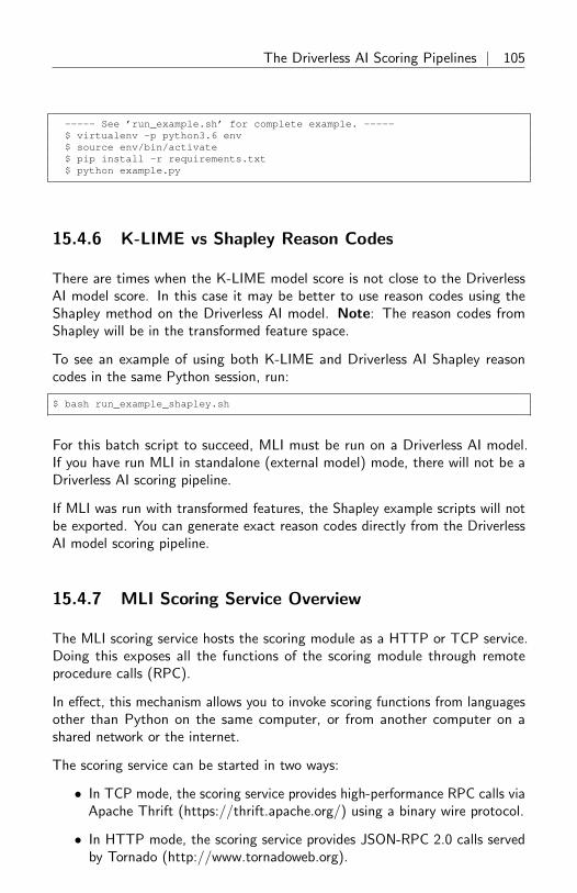
The Driverless AI Scoring Pipelines | 105

----- See ’run_example.sh’ for complete example. -----$ virtualenv -p python3.6 env$ source env/bin/activate$ pip install -r requirements.txt$ python example.py

15.4.6 K-LIME vs Shapley Reason Codes

There are times when the K-LIME model score is not close to the DriverlessAI model score. In this case it may be better to use reason codes using theShapley method on the Driverless AI model. Note: The reason codes fromShapley will be in the transformed feature space.

To see an example of using both K-LIME and Driverless AI Shapley reasoncodes in the same Python session, run:

$ bash run_example_shapley.sh

For this batch script to succeed, MLI must be run on a Driverless AI model.If you have run MLI in standalone (external model) mode, there will not be aDriverless AI scoring pipeline.

If MLI was run with transformed features, the Shapley example scripts will notbe exported. You can generate exact reason codes directly from the DriverlessAI model scoring pipeline.

15.4.7 MLI Scoring Service Overview

The MLI scoring service hosts the scoring module as a HTTP or TCP service.Doing this exposes all the functions of the scoring module through remoteprocedure calls (RPC).

In effect, this mechanism allows you to invoke scoring functions from languagesother than Python on the same computer, or from another computer on ashared network or the internet.

The scoring service can be started in two ways:

• In TCP mode, the scoring service provides high-performance RPC calls viaApache Thrift (https://thrift.apache.org/) using a binary wire protocol.

• In HTTP mode, the scoring service provides JSON-RPC 2.0 calls servedby Tornado (http://www.tornadoweb.org).

106 | The Driverless AI Scoring Pipelines

Scoring operations can be performed on individual rows (row-by-row) usingscore or in batch mode (multiple rows at a time) using score batch. Bothfunctions allow you to specify pred contribs=[True|False] to get MLIpredictions (KLime/Shapley) on a new dataset. See the example shapley.pyfile for more information.

MLI Scoring Service - TCP Mode (Thrift)

The TCP mode allows you to use the scoring service from any language supportedby Thrift, including C, C++, C#, Cocoa, D, Dart, Delphi, Go, Haxe, Java,Node.js, Lua, perl, PHP, Python, Ruby and Smalltalk.

To start the scoring service in TCP mode, you will need to generate the Thriftbindings once, then run the server:

----- See ’run_tcp_server.sh’ for complete example. -----$ thrift --gen py scoring.thrift$ python tcp_server.py --port=9090

Note that the Thrift compiler is only required at build-time. It is not a run timedependency, i.e. once the scoring services are built and tested, you do not needto repeat this installation process on the machines where the scoring servicesare intended to be deployed.

To call the scoring service, simply generate the Thrift bindings for your languageof choice, then make RPC calls via TCP sockets using Thrift’s buffered transportin conjunction with its binary protocol.

----- See ’run_tcp_client.sh’ for complete example. -----$ thrift --gen py scoring.thrift

----- See ’example_client.py’ for complete example. -----socket = TSocket.TSocket(’localhost’, 9090)transport = TTransport.TBufferedTransport(socket)protocol = TBinaryProtocol.TBinaryProtocol(transport)client = ScoringService.Client(protocol)transport.open()row = Row()row.sepalLen = 7.416 # sepal_lenrow.sepalWid = 3.562 # sepal_widrow.petalLen = 1.049 # petal_lenrow.petalWid = 2.388 # petal_widscores = client.score_reason_codes(row)transport.close()

You can reproduce the exact same result from other languages, e.g. Java:

$ thrift --gen java scoring.thrift

// Dependencies:// commons-codec-1.9.jar// commons-logging-1.2.jar// httpclient-4.4.1.jar// httpcore-4.4.1.jar

The Driverless AI Scoring Pipelines | 107

// libthrift-0.10.0.jar// slf4j-api-1.7.12.jar

import ai.h2o.scoring.Row;import ai.h2o.scoring.ScoringService;import org.apache.thrift.TException;import org.apache.thrift.protocol.TBinaryProtocol;import org.apache.thrift.transport.TSocket;import org.apache.thrift.transport.TTransport;import java.util.List;

public class Main {public static void main(String[] args) {try {TTransport transport = new TSocket("localhost", 9090);transport.open();

ScoringService.Client client = new ScoringService.Client(new TBinaryProtocol(transport));

Row row = new Row(7.642, 3.436, 6.721, 1.020);List<Double> scores = client.score_reason_codes(row);System.out.println(scores);

transport.close();} catch (TException ex) {ex.printStackTrace();

}}

}

Scoring Service - HTTP Mode (JSON-RPC 2.0)

The HTTP mode allows you to use the scoring service using plaintext JSON-RPC calls. This is usually less performant compared to Thrift, but has theadvantage of being usable from any HTTP client library in your language ofchoice, without any dependency on Thrift.

For JSON-RPC documentation, see http://www.jsonrpc.org/specification .

To start the scoring service in HTTP mode:

----- See ’run_http_server.sh’ for complete example. -----$ python http_server.py --port=9090

To invoke scoring methods, compose a JSON-RPC message and make a HTTPPOST request to http://host:port/rpc as follows:

----- See ’run_http_client.sh’ for complete example. -----$ curl http://localhost:9090/rpc \--header "Content-Type: application/json" \--data @- <<EOF{"id": 1,"method": "score_reason_codes","params": {"row": [ 7.486, 3.277, 4.755, 2.354 ]

}}

108 | The Driverless AI Scoring Pipelines

EOF

Similarly, you can use any HTTP client library to reproduce the above result.For example, from Python, you can use the requests module as follows:

import requestsrow = [7.486, 3.277, 4.755, 2.354]req = dict(id=1, method=’score_reason_codes’, params=dict(row=row))res = requests.post(’http://localhost:9090/rpc’, data=req)print(res.json()[’result’])

15.5 Driverless AI MOJO Scoring Pipeline

Note: MOJOs are currently not available for TensorFlow or RuleFit models.

For completed experiments, Driverless AI automatically converts models toMOJOs (Model Objects, Optimized), which can be deployed for scoring in realtime. A MOJO is a scoring engine that can be deployed in any Java environmentfor scoring in real time. The MOJO Scoring Pipeline is available as either apure Java solution or a C++-based solution.

Keep in mind that, similar to H2O-3, MOJOs are tied to experiments. Ex-periments and MOJOs are not automatically upgraded when Driverless AI isupgraded.

15.5.1 Prerequisites

The following are required in order to run the MOJO scoring pipeline.

• Java 7 runtime (JDK 1.7) or newer. NOTE: We recommend using Java11+ due to a bug in Java. (See https://bugs.openjdk.java.net/browse/JDK-8186464.)

• Valid Driverless AI license. You can download the license.sig filefrom the machine hosting Driverless AI (usually in the license folder).Copy the license file into the downloaded mojo-pipeline folder.

• mojo2-runtime.jar file. This is available from the top navigation menu inthe Driverless AI UI and in the downloaded mojo-pipeline.zip file for anexperiment.

License Specification

Driverless AI requires a license to be specified in order to run the MOJO ScoringPipeline. The license can be specified in one of the following ways:

• Via an environment variable:

The Driverless AI Scoring Pipelines | 109

– DRIVERLESS AI LICENSE FILE: Path to the Driverless AI li-cense file, or

– DRIVERLESS AI LICENSE KEY: The Driverless AI license key(Base64 encoded string)

• Via a system property of JVM (-D option):

– ai.h2o.mojos.runtime.license.file: Path to the Driver-less AI license file, or

– ai.h2o.mojos.runtime.license.key: The Driverless AIlicense key (Base64 encoded string)

• Via an application classpath:

– The license is loaded from a resource called /license.sig.

– The default resource name can be changed via the JVM systemproperty ai.h2o.mojos.runtime.license.filename.

For example:

# Specify the license via a temporary environment variableexport DRIVERLESS_AI_LICENSE_FILE="path/to/license.sig"

15.5.2 MOJO Scoring Pipeline Files

The mojo-pipeline folder includes the following files:

• run example.sh: A bash script to score a sample test set.

• pipeline.mojo: Standalone scoring pipeline in MOJO format.

• mojo2-runtime.jar: MOJO Java runtime.

• example.csv: Sample test set (synthetic, in the correct format).

• DOT files: Text files that can be rendered as graphs that provide a visualrepresentation of the MOJO scoring pipeline (can be edited to changethe appearance and structure of a rendered graph).

• PNG files: Image files that provide a visual representation of the MOJOscoring pipeline.

15.5.3 Quickstart

Before running the quickstart examples, be sure that the MOJO scoring pipelineis already downloaded and unzipped:

110 | The Driverless AI Scoring Pipelines

1. On the completed Experiment page, click on the Download ScoringPipeline button to download the scorer.zip file for this experiment ontoyour local machine.

Note: This button is Build MOJO Scoring Pipeline if the MOJOScoring Pipeline is disabled.

2. In the pop-up menu that appears, click on the Download MOJO Scor-ing Pipeline button once again to download the scorer.zip file for thisexperiment onto your local machine. Refer to the provided instructionsfor Java, Python, or R.

3. Run the following to score all rows in the sample test set with the filepaths to the test set (example.csv), MOJO pipeline (pipeline.mojo) andlicense (license.sig) stored in environment variables TEST SET FILE,MOJO PIPELINE FILE, DRIVERLESS AI LICENSE KEY:

$ bash run_example.sh

4. Run the following to score a specific test set (example.csv) with MOJOpipeline (pipeline.mojo) and the license file (license.sig):

$ bash run_example.sh pipeline.mojo example.csv license.sig

5. To run Java application for data transformation directly:

$ java -Dai.h2o.mojos.runtime.license.file=license.sig -cp mojo2-runtime.jar ai.h2o.mojos.ExecuteMojo pipeline.mojo example.csv

15.5.4 Execute the MOJO from Java

1. Open a new terminal window, create an experiment folder, and changedirectories to that new folder:

$ mkdir experiment && cd experiment

2. Create your main program in the experiment folder by creating a newfile called Main.java (for example, using vim Main.java). Includethe following contents.

import ai.h2o.mojos.runtime.MojoPipeline;import ai.h2o.mojos.runtime.frame.MojoFrame;import ai.h2o.mojos.runtime.frame.MojoFrameBuilder;import ai.h2o.mojos.runtime.frame.MojoRowBuilder;import ai.h2o.mojos.runtime.lic.LicenseException;

The Driverless AI Scoring Pipelines | 111

import ai.h2o.mojos.runtime.utils.CsvWritingBatchHandler;import com.opencsv.CSVWriter;import java.io.BufferedWriter;import java.io.IOException;import java.io.OutputStreamWriter;import java.io.Writer;

public class DocsExample {public static void main(String[] args) throws IOException,

LicenseException {// Load model and csvfinal MojoPipeline model = MojoPipeline.loadFrom("pipeline.

mojo");

// Get and fill the input columnsfinal MojoFrameBuilder frameBuilder = model.

getInputFrameBuilder();final MojoRowBuilder rowBuilder = frameBuilder.

getMojoRowBuilder();rowBuilder.setValue("AGE", "68");rowBuilder.setValue("RACE", "2");rowBuilder.setValue("DCAPS", "2");rowBuilder.setValue("VOL", "0");rowBuilder.setValue("GLEASON", "6");frameBuilder.addRow(rowBuilder);

// Create a frame which can be transformed by MOJO pipelinefinal MojoFrame iframe = frameBuilder.toMojoFrame();

// Transform input frame by MOJO pipelinefinal MojoFrame oframe = model.transform(iframe);// ‘MojoFrame.debug()‘ can be used to view the contents of

a Frame// oframe.debug();

// Output prediction as CSVfinal Writer writer = new BufferedWriter(new

OutputStreamWriter(System.out));final CSVWriter csvWriter = new CSVWriter(writer);CsvWritingBatchHandler.csvWriteFrame(csvWriter, oframe,

true);}

}

3. Compile the source code with the files of the MOJO runtime (mojo2-runtime.jar) and MOJO pipeline (pipeline.mojo) copied into the experi-ment:

$ javac -cp mojo2-runtime.jar -J-Xms2g -J-XX:MaxPermSize=128m Main.java

4. Run the MOJO example with the license (license.sig) copied into theexperiment:

# Linux and OS X users$ java -Dai.h2o.mojos.runtime.license.file=license.sig -cp .:mojo2-

runtime.jar Main# Windows users$ java -Dai.h2o.mojos.runtime.license.file=license.sig -cp .;mojo2-

runtime.jar Main

112 | The Driverless AI Scoring Pipelines

5. The following output is displayed:

CAPSULE.True0.5442205910902282

15.5.5 MOJO Scoring Pipeline - C++ Solution

The C++ Scoring Pipeline is provided as R and Python packages for theprotobuf-based MOJO2 protocol. The packages are self contained, so noadditional software is required. Simply build the MOJO Scoring Pipeline andbegin using your preferred method. To download the MOJO Scoring Pipelineonto your local machine, click the Download MOJO Scoring Pipeline button,then click the same button again in the pop-up menu that appears. Refer tothe provided instructions for Java, Python, or R.

Notes:

• These scoring pipelines are currently not available for RuleFit models.

• The Download MOJO Scoring Pipeline button appears as BuildMOJO Scoring Pipeline if the MOJO Scoring Pipeline is disabled.

15.5.5.1 Downloading the Scoring Pipeline Runtimes TheR and Python packages can be downloaded from within the Driverless AIapplication. To do this, click Resources, then click MOJO2 R Runtime andMOJO2 Py Runtime from the drop-down menu. In the pop-up menu thatappears, click the button that corresponds to the OS you are using. Choosefrom Linux, Mac OS X, and IBM PowerPC.

Examples

The following examples show how to use the R and Python APIs of the C++MOJO runtime.

R Example

Prerequisites

• Linux OS (x86 or PPC) or Mac OS X (10.9 or newer)

• Driverless AI License (either file or environment variable)

• Rcpp (≥1.0.0)

• data.table

# Install the R MOJO runtime using one of the methods below

# Install the R MOJO runtime on PPC Linux

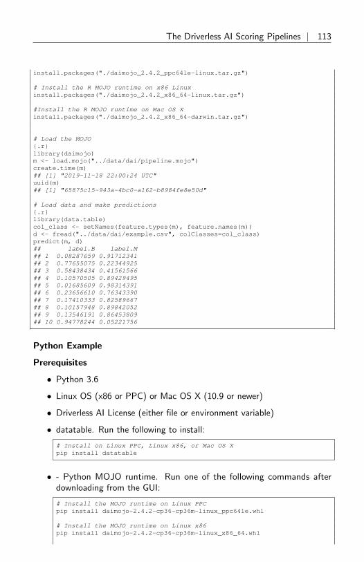
The Driverless AI Scoring Pipelines | 113

install.packages("./daimojo_2.4.2_ppc64le-linux.tar.gz")

# Install the R MOJO runtime on x86 Linuxinstall.packages("./daimojo_2.4.2_x86_64-linux.tar.gz")

#Install the R MOJO runtime on Mac OS Xinstall.packages("./daimojo_2.4.2_x86_64-darwin.tar.gz")

# Load the MOJO{.r}library(daimojo)m <- load.mojo("../data/dai/pipeline.mojo")create.time(m)## [1] "2019-11-18 22:00:24 UTC"uuid(m)## [1] "65875c15-943a-4bc0-a162-b8984fe8e50d"

# Load data and make predictions{.r}library(data.table)col_class <- setNames(feature.types(m), feature.names(m))d <- fread("../data/dai/example.csv", colClasses=col_class)predict(m, d)## label.B label.M## 1 0.08287659 0.91712341## 2 0.77655075 0.22344925## 3 0.58438434 0.41561566## 4 0.10570505 0.89429495## 5 0.01685609 0.98314391## 6 0.23656610 0.76343390## 7 0.17410333 0.82589667## 8 0.10157948 0.89842052## 9 0.13546191 0.86453809## 10 0.94778244 0.05221756

Python Example

Prerequisites

• Python 3.6

• Linux OS (x86 or PPC) or Mac OS X (10.9 or newer)

• Driverless AI License (either file or environment variable)

• datatable. Run the following to install:

# Install on Linux PPC, Linux x86, or Mac OS Xpip install datatable

• - Python MOJO runtime. Run one of the following commands afterdownloading from the GUI:

# Install the MOJO runtime on Linux PPCpip install daimojo-2.4.2-cp36-cp36m-linux_ppc64le.whl

# Install the MOJO runtime on Linux x86pip install daimojo-2.4.2-cp36-cp36m-linux_x86_64.whl

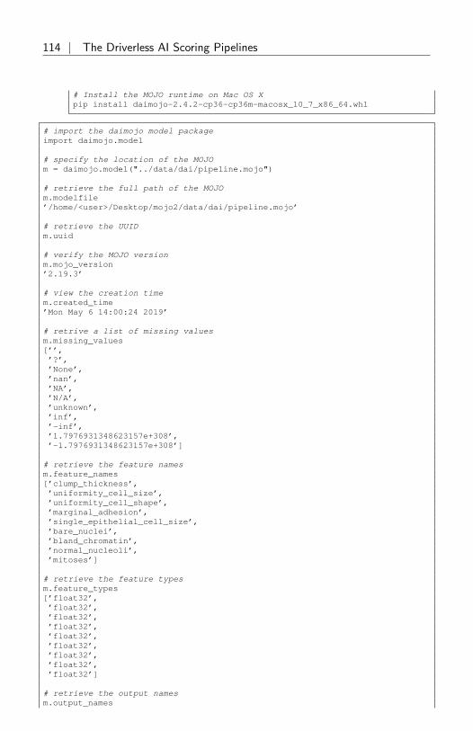
114 | The Driverless AI Scoring Pipelines

# Install the MOJO runtime on Mac OS Xpip install daimojo-2.4.2-cp36-cp36m-macosx_10_7_x86_64.whl

# import the daimojo model packageimport daimojo.model

# specify the location of the MOJOm = daimojo.model("../data/dai/pipeline.mojo")

# retrieve the full path of the MOJOm.modelfile’/home/<user>/Desktop/mojo2/data/dai/pipeline.mojo’

# retrieve the UUIDm.uuid

# verify the MOJO versionm.mojo_version’2.19.3’

# view the creation timem.created_time’Mon May 6 14:00:24 2019’

# retrive a list of missing valuesm.missing_values[’’,’?’,’None’,’nan’,’NA’,’N/A’,’unknown’,’inf’,’-inf’,’1.7976931348623157e+308’,’-1.7976931348623157e+308’]

# retrieve the feature namesm.feature_names[’clump_thickness’,’uniformity_cell_size’,’uniformity_cell_shape’,’marginal_adhesion’,’single_epithelial_cell_size’,’bare_nuclei’,’bland_chromatin’,’normal_nucleoli’,’mitoses’]

# retrieve the feature typesm.feature_types[’float32’,’float32’,’float32’,’float32’,’float32’,’float32’,’float32’,’float32’,’float32’]

# retrieve the output namesm.output_names

Deployment | 115

[’label.B’, ’label.M’]

# retrieve the output types[’float64’, ’float64’]

# import the datatable moduleimport datatable as dt

# parse the example.csv filepydt = dt.fread("../data/dai/example.csv", na_strings=m.missing_values)

# retrieve the column typespydt.stypes(stype.float64,stype.float64,stype.float64,stype.float64,stype.float64,stype.float64,stype.float64,stype.float64,stype.float64)

# make predictions on the example.csv fileres = m.predict(pydt)

# retrieve the predictionsres

label.B. label.M0 0.0828766 0.9171231 0.776551 0.2234492 0.584384 0.4156163 0.105705 0.8942954 0.0168561 0.9831445 0.236566 0.7634346 0.174103 0.8258977 0.101579 0.8984218 0.135462 0.8645389 0.947782 0.0522176

[10 rows by 2 columns]

# retrieve the prediction column namesres.names# (’label.B’, ’label.M’)

# retrieve the prediction column typesres.stypes(stype.float64, stype.float64)

# convert datatable results to common data types# res.to_pandas() # need pandas# res.to_numpy() # need numpyres.to_list()

16 DeploymentDriverless AI can deploy the MOJO scoring pipeline for you to test and/or tointegrate into a final product.

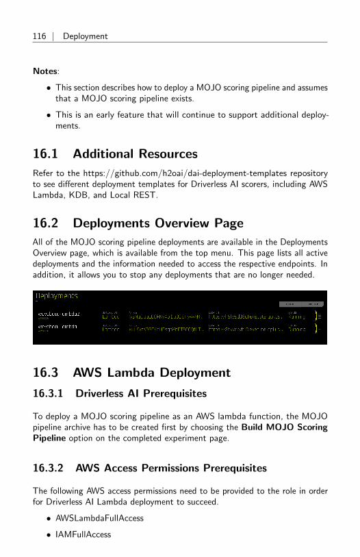
116 | Deployment

Notes:

• This section describes how to deploy a MOJO scoring pipeline and assumesthat a MOJO scoring pipeline exists.

• This is an early feature that will continue to support additional deploy-ments.

16.1 Additional Resources

Refer to the https://github.com/h2oai/dai-deployment-templates repositoryto see different deployment templates for Driverless AI scorers, including AWSLambda, KDB, and Local REST.

16.2 Deployments Overview Page

All of the MOJO scoring pipeline deployments are available in the DeploymentsOverview page, which is available from the top menu. This page lists all activedeployments and the information needed to access the respective endpoints. Inaddition, it allows you to stop any deployments that are no longer needed.

16.3 AWS Lambda Deployment

16.3.1 Driverless AI Prerequisites

To deploy a MOJO scoring pipeline as an AWS lambda function, the MOJOpipeline archive has to be created first by choosing the Build MOJO ScoringPipeline option on the completed experiment page.

16.3.2 AWS Access Permissions Prerequisites

The following AWS access permissions need to be provided to the role in orderfor Driverless AI Lambda deployment to succeed.

• AWSLambdaFullAccess

• IAMFullAccess

Deployment | 117

• AmazonAPIGatewayAdministrator

The policy can be further stripped down to restrict Lambda and S3 rights usingthe JSON policy definition as follows:

{"Version": "2012-10-17","Statement": [

{"Sid": "VisualEditor0","Effect": "Allow","Action": [

"iam:GetPolicyVersion","iam:DeletePolicy","iam:CreateRole","iam:AttachRolePolicy","iam:ListInstanceProfilesForRole","iam:PassRole","iam:DetachRolePolicy","iam:ListAttachedRolePolicies","iam:GetRole","iam:GetPolicy","iam:DeleteRole","iam:CreatePolicy","iam:ListPolicyVersions"

],"Resource": [

"arn:aws:iam::*:role/h2oai*","arn:aws:iam::*:policy/h2oai*"

]},{

"Sid": "VisualEditor1","Effect": "Allow","Action": "apigateway:*","Resource": "*"

},{

"Sid": "VisualEditor2","Effect": "Allow","Action": [

"lambda:CreateFunction","lambda:ListFunctions","lambda:InvokeFunction","lambda:GetFunction","lambda:UpdateFunctionConfiguration","lambda:DeleteFunctionConcurrency","lambda:RemovePermission","lambda:UpdateFunctionCode","lambda:AddPermission","lambda:ListVersionsByFunction",

118 | Deployment

"lambda:GetFunctionConfiguration","lambda:DeleteFunction","lambda:PutFunctionConcurrency","lambda:GetPolicy"

],"Resource": "arn:aws:lambda:*:*:function:h2oai*"

},{

"Sid": "VisualEditor3","Effect": "Allow","Action": "s3:*","Resource": [

"arn:aws:s3:::h2oai*/*","arn:aws:s3:::h2oai*"

]}

]}

16.3.3 Deploying the Lambda

Once the MOJO pipeline archive is ready, Driverless AI provides a Deployoption on the completed experiment page.

Note: This button is not available on PPC64LE environments.

This option opens a new dialog for setting the AWS account credentials (or usethose supplied in the Driverless AI configuration file or environment variables),AWS region, and the desired deployment name (which must be unique perDriverless AI user and AWS account used).

Amazon Lambda deployment parameters:

• Deployment Name: A unique name of the deployment. By default,Driverless AI offers a name based on the name of the experiment and thedeployment type. This has to be unique both for Driverless AI user andthe AWS account used.

• Region: The AWS region to deploy the MOJO scoring pipeline to. Itmakes sense to choose a region geographically close to any client codecalling the endpoint in order to minimize request latency. (See also AWSRegions and Availability Zones.)

Deployment | 119

• Use AWS environment variables: If enabled, the AWS credentials aretaken from the Driverless AI configuration file. This would usually beentered by the Driverless AI installation administrator.

• AWS Access Key ID and AWS Secret Access Key: Credentials toaccess the AWS account. This pair of secrets identifies the AWS userand the account and can be obtained from the AWS account console.

16.3.4 Testing the Lambda Deployment

On a successful deployment, all the information needed to access the newendpoint (URL and an API Key) is printed, and the same information is availablein the Deployments Overview Page after clicking on the deployment row.

Note that the actual scoring endpoint is located at the path /score. In addition,to prevent DDoS and other malicious activities, the resulting AWS lambda isprotected by an API Key, i.e., a secret that has to be passed in as a part of therequest using the x-api-key HTTP header.

The request is a JSON object containing attributes:

• fields: A list of input column names that should correspond to the trainingdata columns.

• rows: A list of rows that are in turn lists of cell values to predict thetarget values for.

• (optional) includeFieldsInOutput: A list of input columns that shouldbe included in the output.

An example request providing 2 columns on the input and asking to get onecolumn copied to the output looks as follows:

{"fields": ["age", "salary"

],"includeFieldsInOutput": ["salary"

120 | Deployment

],"rows": [["48.0", "15000.0"

],["35.0", "35000.0"

],["18.0", "22000.0"

]]

}

Assuming the request is stored locally in a file named test.json, the request tothe endpoint can be sent, e.g., using the curl utility, as follows:

$ URL={place the endpoint URL here}$ API_KEY={place the endpoint API key here}$ curl \

-X POST \-H "x-api-key: ${API_KEY}" \-d @test.json ${URL}/score

The response is a JSON object with a single attribute “score“, which containsthe list of rows with the optional copied input values and the predictions.

For the example above with a two class target field, the result is likely to looksomething like the following snippet. The particular values would of coursedepend on the scoring pipeline:

{"score": [["48.0","0.6240277982943945","0.045458571508101536",

],["35.0","0.7209441819603676","0.06299909138586585",

],["18.0","0.7209441819603676","0.06299909138586585",

]]

}

16.3.5 AWS Deployment Issues

We create a new S3 bucket per AWS Lambda deployment. The bucket nameshave to be unique throughout AWS S3, and one user can create a maximum

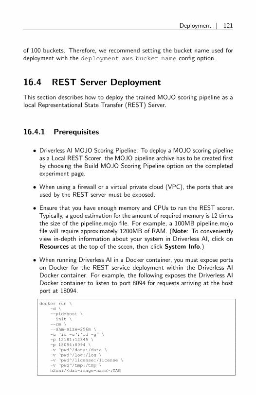
Deployment | 121

of 100 buckets. Therefore, we recommend setting the bucket name used fordeployment with the deployment aws bucket name config option.

16.4 REST Server Deployment

This section describes how to deploy the trained MOJO scoring pipeline as alocal Representational State Transfer (REST) Server.

16.4.1 Prerequisites

• Driverless AI MOJO Scoring Pipeline: To deploy a MOJO scoring pipelineas a Local REST Scorer, the MOJO pipeline archive has to be created firstby choosing the Build MOJO Scoring Pipeline option on the completedexperiment page.

• When using a firewall or a virtual private cloud (VPC), the ports that areused by the REST server must be exposed.

• Ensure that you have enough memory and CPUs to run the REST scorer.Typically, a good estimation for the amount of required memory is 12 timesthe size of the pipeline.mojo file. For example, a 100MB pipeline.mojofile will require approximately 1200MB of RAM. (Note: To convenientlyview in-depth information about your system in Driverless AI, click onResources at the top of the sceen, then click System Info.)

• When running Driverless AI in a Docker container, you must expose portson Docker for the REST service deployment within the Driverless AIDocker container. For example, the following exposes the Driverless AIDocker container to listen to port 8094 for requests arriving at the hostport at 18094.

docker run \-d \--pid=host \--init \--rm \--shm-size=256m \-u ‘id -u‘:‘id -g‘ \-p 12181:12345 \-p 18094:8094 \-v ‘pwd‘/data:/data \-v ‘pwd‘/log:/log \-v ‘pwd‘/license:/license \-v ‘pwd‘/tmp:/tmp \h2oai/<dai-image-name>:TAG

122 | Deployment

16.4.2 Deploying on REST Server

Once the MOJO pipeline archive is ready, Driverless AI provides a Deploy(Local & Cloud) option on the completed experiment page.

Notes: This button is only available after the MOJO Scoring Pipeline has beenbuilt.

This option opens a new dialog for setting the REST Server deployment name,port number, and maximum heap size (optional).

1. Specify a name for the REST scorer in order to help track the deployedREST scorers.

Deployment | 123

2. Provide a port number on which the REST scorer will run. For example,if port number 8081 is selected, the scorer will be available at http://my-ip-address:8081/models

3. Optionally specify the maximum heap size for the Java Virtual Machine(JVM) running the REST scorer. This can help constrain the REST scorerfrom overconsuming memory of the machine. Because the REST scoreris running on the same machine as Driverless AI, it may be helpful tolimit the amount of memory that is allocated to the REST scorer. Thisoption will limit the amount of memory the REST scorer can use, but itwill also produce an error if the memory allocated is not enough to runthe scorer. (The amount of memory required is mostly dependent on thesize of MOJO. See Prerequisites for more information.)

16.4.3 Testing the REST Server Deployment

The request is a JSON object containing attributes:

• fields: A list of input column names that should correspond to the trainingdata columns.

• rows: A list of rows that are in turn lists of cell values to predict thetarget values for.

• (optional) includeFieldsInOutput: A list of input columns that shouldbe included in the output.

An example request providing 2 columns on the input and asking to get onecolumn copied to the output looks as follows:

124 | Deployment

{"fields": ["age", "salary"

],"includeFieldsInOutput": ["salary"

],"rows": [["48.0", "15000.0"

],["35.0", "35000.0"

],["18.0", "22000.0"

]]

}

Assuming the request is stored locally in a file named test.json, the requestto the endpoint can be sent, e.g., using the curl utility, as follows:

URL={place the endpoint URL here}curl \-X POST \-d {"fields": [’age’, ’salary’, ’education’], "rows": [1, 2, 3], "

includeFieldsInOutput": ["education"]}\-H "Content-Type: application/json" \${URL}/score

The response is a JSON object with a single attribute score, which containsthe list of rows with the optional copied input values and the predictions.

For the example above with a two class target field, the result is likely to looksomething like the following snippet (the exact values depend on the scoringpipeline):

{"score": [["48.0","0.6240277982943945","0.045458571508101536",

],["35.0","0.7209441819603676","0.06299909138586585",

],["18.0","0.7209441819603676","0.06299909138586585",

]]

}

About Driverless AI Transformations | 125

16.4.4 REST Server Deployment Issues

• Local REST server deployments are useful for determining the behavioralcharacteristics of a MOJO that is intended for deployment. However, wedon’t recommend using the REST Server deployment as a production levelscoring service. The REST Server deployment runs in the same machine asthe core of Driverless AI, and therefore has to share system resources withall other Driverless AI processes. This can lead to unexpected scenarios inwhich competition for compute resources causes the REST Server to fail.

Additionally, given that the memory and CPU resource requirements forthe REST scorer and for scoring the MOJO are typically smaller thanthe requirements for training, it is typically much more cost effectiveto deploy the MOJO in a smaller instance/machine. Templates can beeasily found/built from the repository: https://github.com/h2oai/dai-deployment-templates.

• The REST Server will be shut down if Driverless AI is restarted.

17 About Driverless AI Transformations

Transformations in Driverless AI are applied to columns in the data. Thetransformers create the engineered features in experiments.

Driverless AI provides a number of transformers. The downloaded experimentlogs include the transformations that were applied to your experiment. Notethat you can exclude transformations in the config.toml file, and that list ofexcluded transformers will also be available in the experiment log.

The following transformers are available for classification (multiclass and binary)and regression experiments.

17.1 Numeric Transformers

• ClusterDist Transformer: The Cluster Distance Transformer clustersselected numeric columns and uses the distance to a specific cluster as anew feature.

• ClusterTE Transformer: The Cluster Target Encoding Transformerclusters selected numeric columns and calculates the mean of the responsecolumn for each cluster. The mean of the response is used as a newfeature. Cross Validation is used to calculate mean response to preventoverfitting.

126 | About Driverless AI Transformations

• Interactions Transformer: The Interactions Transformer adds, divides,multiplies, and subtracts two numeric columns in the data to create anew feature. This transformation uses a smart search to identify whichfeature pairs to transform. Only interactions that improve the baselinemodel score are kept.

• InteractionsSimple Transformer: The InteractionsSimple Transformeradds, divides, multiplies, and subtracts two numeric columns in the datato create a new feature. This transformation randomly selects pairs offeatures to transform.

• NumCatTE Transformer: The Numeric Categorical Target EncodingTransformer calculates the mean of the response column for severalselected columns. If one of the selected columns is numeric, it is firstconverted to categorical by binning. The mean of the response columnis used as a new feature. Cross Validation is used to calculate meanresponse to prevent overfitting.

• NumToCatTE Transformer: The Numeric to Categorical Target En-coding Transformer converts numeric columns to categoricals by binningand then calculates the mean of the response column for each group.The mean of the response for the bin is used as a new feature. CrossValidation is used to calculate mean response to prevent overfitting.

• NumToCatWoEMonotonic Transformer: The Numeric to CategoricalWeight of Evidence Transformer converts a numeric column to categoricalby binning and then calculates Weight of Evidence for each bin. TheWeight of Evidence is used as a new feature. Weight of Evidence measuresthe strength of a grouping for separating good and bad risk and iscalculated by taking the log of the ratio of distributions for a binaryresponse column.

• NumToCatWoE Transformer: The Numeric to Categorical Weight ofEvidence Transformer converts a numeric column to categorical by binningand then calculates Weight of Evidence for each bin. The Weight ofEvidence is used as a new feature. Weight of Evidence measures thestrength of a grouping for separating good and bad risk and is calculatedby taking the log of the ratio of distributions for a binary response column.

• Original Transformer: The Original Transformer applies an identitytransformation to a numeric column.

• TruncSVDNum Transformer: Truncated SVD Transformer trains aTruncated SVD model on selected numeric columns and uses the compo-nents of the truncated SVD matrix as new features.

About Driverless AI Transformations | 127

17.2 Time Series Experiments Transformers

• DateOriginal Transformer: The Date Original Transformer retrievesdate values such as year, quarter, month, day, day of the year, week, andweekday values.

• DateTimeOriginal Transformer: The Date Original Transformer re-trieves date values such as year, quarter, month, day, day of the year,week, and weekday values.

• EwmaLags Transformer: The Exponentially Weighted Moving Aver-age (EWMA) Transformer calculates the exponentially weighted movingaverage of target or feature lags.

• LagsAggregates Transformer: The Lags Aggregates Transformer cal-culates aggregations of target/feature lags like mean(lag7, lag14, lag21)with support for mean, min, max, median, sum, skew, kurtosis, std. Theaggregation is used as a new feature.

• LagsInteraction Transformer: The Lags Interaction Transformer createstarget/feature lags and calculates interactions between the lags (lag2 -lag1, for instance). The interaction is used as a new feature.

• Lags Transformer: The Lags Transformer creates target/feature lags,possibly over groups. Each lag is used as a new feature. Lag transformersmay apply to categorical (strings) features or binary/multiclass stringvalued targets after they have been internally numerically encoded.

• LinearLagsRegression Transformer: The Linear Lags Regression trans-former trains a linear model on the target or feature lags to predict thecurrent target or feature value. The linear model prediction is used as anew feature.

17.3 Categorical Transformers (String)

• Cat Transformer: The Cat Transformer sorts a categorical column inlexicographical order and uses the order index created as a new feature.

• CatOriginal Transformer: The Categorical Original Transformer appliesan identity transformation that leaves categorical features as they are.This transformer works with models that can handle non-numeric featurevalues.

• CVCatNumEncode Transformer: The Cross Validation Categorical toNumeric Encoding Transformer calculates an aggregation of a numericcolumn for each value in a categorical column (ex: calculate the meanTemperature for each City) and uses this aggregation as a new feature.

128 | About Driverless AI Transformations

• CVTargetEncode Transformer: The Cross Validation Target EncodingTransformer calculates the mean of the response column for each valuein a categorical column and uses this as a new feature. Cross Validationis used to calculate mean response to prevent overfitting.

• Frequent Transformer: The Frequent Transformer calculates the fre-quency for each value in categorical column(s) and uses this as a newfeature. This count can be either the raw count or the normalized count.

• LexiLabelEncoder Transformer: The Lexi Label Encoder sorts a cate-gorical column in lexicographical order and uses the order index createdas a new feature.

• NumCatTE Transformer: The Numeric Categorical Target EncodingTransformer calculates the mean of the response column for severalselected columns. If one of the selected columns is numeric, it is firstconverted to categorical by binning. The mean of the response columnis used as a new feature. Cross Validation is used to calculate meanresponse to prevent overfitting.

• OneHotEncoding Transformer: The One-hot Encoding transformerconverts a categorical column to a series of boolean features by performingone-hot encoding. The boolean features are used as new features.

• SortedLE Transformer: The Sorted Label Encoding Transformer sortsa categorical column by the response column and uses the order indexcreated as a new feature.

• WeightOfEvidence Transformer: The Weight of Evidence Transformercalculates Weight of Evidence for each value in categorical column(s).The Weight of Evidence is used as a new feature. Weight of Evidencemeasures the strength of a grouping for separating good and bad risk andis calculated by taking the log of the ratio of distributions for a binaryresponse column.

This only works with a binary target variable. The likelihood needs to becreated within a stratified kfold if a fit transform method is used. Moreinformation can be found here: http://ucanalytics.com/blogs/information-value-and-weight-of-evidencebanking-case/.

About Driverless AI Transformations | 129

17.4 Text Transformers (String)

• TextBiGRU Transformer: The Text Bidirectional GRU Transformertrains a bi-directional GRU TensorFlow model on word embeddings createdfrom a text feature to predict the response column. The GRU predictionis used as a new feature. Cross Validation is used when training the GRUmodel to prevent overfitting.

• TextCharCNN Transformer: The Text Character CNN Transformertrains a CNN TensorFlow model on character embeddings created from atext feature to predict the response column. The CNN prediction is usedas a new feature. Cross Validation is used when training the CNN modelto prevent overfitting.

• TextCNN Transformer: The Text CNN Transformer trains a CNNTensorFlow model on word embeddings created from a text feature topredict the response column. The CNN prediction is used as a new afeature. Cross Validation is used when training the CNN model to preventoverfitting.

• TextLinModel Transformer: The Text Linear Model Transformer trainsa linear model on a TF-IDF matrix created from a text feature to predictthe response column. The linear model prediction is used as a newfeature. Cross Validation is used when training the linear model toprevent overfitting.

• Text Transformer: The Text Transformer tokenizes a text column andcreates a TFIDF matrix (term frequency-inverse document frequency)or count (count of the word) matrix. This may be followed by dimen-sionality reduction using truncated SVD. Selected components of theTF-IDF/Count matrix are used as new features.

17.5 Time Transformers (Date, Time)

• Dates Transformer: The Dates Transformer retrieves any date values,including year, quarter, month, day, day of the year, week, weekday, hour,minute, and second values.

• IsHoliday Transformer: The Is Holiday Transformer determines if a datecolumn is a holiday. A boolean column indicating if the date is a holidayis added as a new feature. Creates a separate feature for holidays in theUnited States, United Kingdom, Germany, Mexico, and the EuropeanCentral Bank. Other countries available in the python Holiday packagecan be added via the configuration file.

130 | Logs

18 Logs

Driverless AI provides a number of logs that can be retrieved while visualizingdatasets, while an experiment is running, and after an experiment is completed.

While Visualizing Datasets

When running Autovisualization, you can access the Autoviz logs by clickingthe Display Logs button on the Visualize Datasets page.

This page presents logs created while the dataset visualization was beingperformed. You can download the vis-data-server.log file by clicking theDownload Logs button on this page. This file can be used to troubleshootany issues encountered during dataset visualization.

While an Experiment is Running

While the experiment is running, you can access the logs by clicking on theLog button on the experiment screen. The Log button can be found in theCPU/Memory section. Clicking on the Log button will present the experimentlogs in real time. You can download these logs by clicking on the DownloadLogs button in the upper right corner.

Logs | 131

Only the h2oai experiment.log will be downloaded while the experiment isrunning (for example: h2oai experiment tobosoru.log). It will have the sameinformation as the logs being presented in real time on the screen.

For troubleshooting purposes, view the complete h2oai experiment.log (orh2oai experiment anonymized.log). This will be available after the experi-ment finishes, as described in the next section.

After an Experiment has Finished

If the experiment has finished, you can download the logs by clicking on theDownload Summary and Logs button at the center of the experiment screen.

This will download a zip file which includes the following logs:

• h2oai experiment.log: This is the log corresponding to the experiment.

• h2oai experiment anonymized.log: This is the log corresponding tothe experiment where all data in the log is anonymized.

• h2oai server.log: Contains the logs for all experiments and all users.

• h2oai server anonymized.log: Contains the logs for all experimentsand all users where all data in the log is anonymized.

• h2o.log: This is the log corresponding to H2O-3. (H2O-3 is usedinternally for parts of Driverless AI.)

132 | Logs

For troubleshooting purposes, view the complete h2oai experiment.log or theh2oai experiment anonymized.log.

The following additional information about your particular experiment will alsobe included in the zip file:

• tuning leaderboard.txt: The results of the parameter tuning stage. Thiscontains the model parameters investigated and their performance.

• gene summary.txt: A summary of the feature transformations availablefor each gene over the feature engineering iterations

• features.txt: The features used in the final Driverless AI model alongwith feature importance and feature description

• details folder: Contains standard streams for each of the subprocessesperformed by Driverless A. This information is for debugging purposes

After Model Interpretation

You can view an MLI log for completed model interpretations by selecting theDownload MLI Logs link on the MLI page.

This will download a zip file which includes the following logs:

• h2oai experiment mli key.log: This is the log corresponding to the modelinterpretation.

• h2oai experiment mli key anonymized.log: This is the log correspondingto the model interpretation where all data in the log is anonymized.

This file can be used to view logging information for successful interpretations.If MLI fails, then those logs are in ./tmp/h2oai experiment mli key.log and./tmp/h2oai experiment mli key anonymized.log.

References | 133

18.1 Sending Logs to H2O

This section describes the logs to send in the event of failures when runningDriverless AI.

Dataset Failures

• Adding Datasets: If a dataset fails to import, a message on the screenshould provide the reason for the failure. The logs to send are availablein the Driverless AI ./tmp folder.

• Dataset Details: If a failure occurs when attempting to view DatasetDetails, the logs to send are available in the Driverless AI ./tmp folder.

• Autovisualization: If a failure occurs when attempting to VisualizeDatasets, a message on the screen should provide a reason for the failure.The logs to send are available in the Driverless AI ./tmp folder.

Experiments

• While Running an Experiment: As indicated previously, a Log buttonis available on the Experiment page. Clicking on the Log button willpresent the experiment logs in real time. You can download these logsby clicking on the Download Logs button in the upper right corner.You can also retrieve the h2oai experiment.log for the correspondingexperiment in the Driverless AI ./tmp folder.

MLI

• During Model Interpretation: If a failure occurs during model interpre-tation, then the logs to send are ./tmp/h2oai experiment mli key.logand ./tmp/h2oai experiment mli key anonymized.log.

19 References

1. L. Breiman. Statistical modeling: The two cultures (with commentsand a rejoinder by the author). Statistical Science, 16(3), 2001. URLhttps://projecteuclid.org/euclid.ss/1009213726

2. M. W. Craven and J. W. Shavlik. Extracting tree-structured represen-tations of trained networks. Advances in Neural Information Process-ing Systems, 1996. URL http://papers.nips.cc/paper/1152-extracting-tree-structured-representations-of-trained-networks.pdf

134 | References

3. J. Friedman. Predictive Learning via Rule Ensembles, October 2005.URL http://statweb.stanford.edu/˜jhf/ftp/RuleFit.pdf

4. J. Friedman, T. Hastie, and R. Tibshirani. The Elements of StatisticalLearning. Springer, New York, 2001. URL https://web.stanford.edu/˜hastie/ElemStatLearn/printings/ESLII_print12.pdf

5. A. Goldstein, A. Kapelner, J. Bleich, and E. Pitkin. Peeking inside the blackbox: Visualizing statistical learning with plots of individual conditionalexpectation. Journal of Computational and Graphical Statistics, 24(1),2015

6. R. A. Groeneveld and G. Meeden. Measuring Skewness and Kurtosis.Journal of the Royal Statistical Society. Series D (The Statistician), 33(4):391–399, December 1984

7. P. Hall, W. Phan, and S. S. Ambati. Ideas on interpreting machinelearning. O’Reilly Ideas, 2017. URL https://www.oreilly.com/ideas/ideas-on-interpreting-machine-learning

8. J. Hartigan and S. Mohanty. The RUNT test for Multimodality.Journal of Classification, 9(1):63–70, January 1992

9. J. Lei, M. G’Sell, A. Rinaldo, R. J. Tibshirani, and L. Wasserman.Distribution-free predictive inference for regression. Journal of the Amer-ican Statistical Association just-accepted, 2017. URL http://www.stat.cmu.edu/˜ryantibs/papers/conformal.pdf

10. H. B. McMahan, G. Holt, D. Sculley, M. Young, D. Ebner, J. Grady, L. Nie,T. Phillips, E. Davydov, D. Golovin, S. Chikkerur, D. Liu, M. Wattenberg,A. M. Hrafnkelsson, T. Boulos, and J. Kubica. Ad Click Prediction: AView from the Trenches. In Proceedings of the 19th ACM SIGKDDinternational conference on Knowledge discovery and data mining, 2013.URL https://research.google.com/pubs/archive/41159.pdf

11. F. Niu, B. Recht, C. Re, and S. J. Wright. Hogwild!: A Lock-FreeApproach to Parallelizing Stochastic Gradient Descent. In NIPS,2011. URL https://people.eecs.berkeley.edu/˜brecht/papers/hogwildTR.pdf

12. M. T. Ribeiro, S. Singh, and C. Guestrin. Why should I trust you?:Explaining the predictions of any classifier. In Proceedings of the 22ndACM SIGKDD International Conference on Knowledge Discovery andData Mining, pages 1135–1144. ACM, 2016. URL http://www.kdd.org/kdd2016/papers/files/rfp0573-ribeiroA.pdf

Authors | 135

13. J. W. Tukey. Exploratory Data Analysis. Addison-Wesley, Reading,MA, 1977

14. L. Wilkinson. Dot Plots. The American Statistician, 53(3):276–281,1999

15. L. Wilkinson, A. Anand, and R. Grossman. ”Graph-theoretic Scagnostics,”in Proceedings of the IEEE Information Visualization. INFOVIS ’05. IEEEComputer Society, Washington, DC, USA, 2005

16. I. Yeo and R. Johnson. A new family of power transformations to improvenormality or symmetry. Biometrika, 2000. URL https://www.jstor.org/stable/2673623?seq=1

17. H2O.ai Team. Datatable for python. URL https://github.com/h2oai/datatable

20 AuthorsPatrick Hall

Patrick Hall is senior director for data science products at H2O.ai where hefocuses mainly on model interpretability. Patrick is also currently an adjunctprofessor in the Department of Decision Sciences at George Washington Univer-sity, where he teaches graduate classes in data mining and machine learning.Prior to joining H2O.ai, Patrick held global customer facing roles and researchand development roles at SAS Institute.

Follow him on Twitter: @jpatrickhall

Megan Kurka

Megan is a customer data scientist at H2O.ai. Prior to working at H2O.ai,she worked as a data scientist building products driven by machine learning forB2B customers. Megan has experience working with customers across multipleindustries, identifying common problems, and designing robust and automatedsolutions.

Angela Bartz

Angela is the doc whisperer at H2O.ai. With extensive experience in technicalcommunication, she brings our products to life by documenting the features andfunctionality of the entire suite of H2O products. Having worked for companiesboth large and small, she is an expert at understanding her audience andtranslating complex ideas into consumable documents. Angela has a BA degreein English from the University of Detroit Mercy.