USING MICROCOMPUTERS AND P/G% TO PREDICTCOURT CASES

by

STUART S. NAGEL*

The purpose of this article is to analyze a microcomputer program thatcan process a set of (1) prior cases, (2) predictive criteria for distinguishingamong the cases, and (3) the relations between each prior case and eachcriterion in order to arrive at an accurate decision rule. Such a rule will enableall the prior cases to be predicted without inconsistencies, and thereby max-imize the likelihood of accurately predicting future cases. To illustrate the pro-gram, this article uses five substantive fields, including the predicting of casesdealing with religion in the public schools, legislative redistricting, housingdiscrimination, international law, and criminal law.!

THE GENERAL METHODOLOGY

The predictive methodology on which the computer program is based in-volves six key elements:

1. Listing the cases or casetypes which are to be analyzed.2. Listing the tentative criteria to aid in explaining why some cases were

decided one way and other cases were decided differently. That listingmight also involve indicating the relative importance of each criterion.

3. Listing how each case scores on each of those predictive criteria. Thatlisting can use whatever measurement units seem comfortable, such asa yes-no dichotomy, a 1-5 scale, years, dollars, apples, etc.

4. Summing the scores for each case across the criteria in order to giveeach case an overall score. Doing so might involve transforming theraw scores into dimensionless part/whole percentages.

5. Relating the set of summation scores for the cases to the actual orpresumed outcomes of those past cases or casetypes. One can therebydevelop a decision rule indicating the summation scores that areassociated with certain kinds of outcomes.

6. Doing a sensitivity analysis whereby one determines how the decisionrule, the presence of inconsistencies, or a litigation strategy might beaffected by changes in the cases, criteria, weights, relations, measure-ment units, or other inputs.

*Professor of Political Science, University of Illinois; member of the Illinois Bar. B.S., 1957, J.D., 1958,Ph.D., 1961, Northwestern University.'On traditional legal prediction, see H. JONES, J. KERNOCHAN & A. MURPHY, LEGAL METHOD (1980); K.LLEWELLYN, THE COMMON LAW TRADITION: DECIDING APPEALS (1960); W. STATSKY & J. WERNET, CASEANALYSIS AND FUNDAMENTALS OF LEGAL WRITING (1977); and E. THODE, L. LEBowITz & L. MAZOR, IN.TRODUCTION TO THE STUDY OF LAw (1970). On behavioral statistical prediction as applied to court cases, seeJ. GROSSMAN & J. TANENHAUS, FRONTIERS OF JUDICIAL RESEARCH (1969); G. SCHUBERT, JUDICAL BEHAVIOR:

541

AKRON LAW REVIEW

The program is called Policy/Goal Percentaging Analysis (PIG%) becauseit was originally designed to relate alternative legal policies to goals to beachieved. The program can be easily extended to relating prior cases to predic-tive criteria. The word "percentaging" is used in the title of the program,because the program uses part/whole percentages in order to handle the prob-lem of goals or predictive criteria being measured on different dimensions. Themeasurement units are converted into a system of percentages showing therelative position of each case on each criterion, rather than work with a systemof dollars, apples, years, miles, or other measurement scores.

Each set of substantive cases is designed to illustrate a different variationon the six key elements as follows:

1. The cases dealing with religion in the public schools involve casetypes,rather than actual cases. They also involve only one way of measuringthe predictive criteria, namely a simple yes-no dichotomy.

2. The legislative redistricting cases involve specific cases, rather thancasetypes. They especially illustrate resolving inconsistencies in howthe cases were decided.

3. The housing discrimination cases illustrate how the program dealswith multiple ways of measuring the predictive criteria.

4. The international law cases involve a continuum outcome like dam-ages, sentences, or probabilities, rather than just winning or losing.

5. The criminal cases deal with multiple weights for the predictivecriteria.

This article is designed to discuss a methodology that is helpful in arrivingat accurate predictions of court cases. Making accurate predictions, however,depends on a number of factors in addition to having a good predictivemethodology. Those factors include:

1. A knowledge of the subject matter.2. Previous prediction experiences.3. The Stimulus of having a lot at stake, depending on the accuracy of

the predictions.4. Requiring written analysis justifying one's predictions.5. Clarity as to what one is predicting.6. Being a positive thinker with regard to one's ability to predict.7. Being explicit about one's predictive criteria.8. Having a relevant set of cases on which to base one's predictions.9. Being accurate in how the cases are positioned on each of the predic-

tive criteria.10. Being capable of seeing relations and reasoning by analogy.

A READER IN THEORY AND RESEARCH (1964); H. SPAETH, SUPREME COURT POLICY MAKING: EXPLANATIONAND PREDICTION (1979); and S. ULMER, COURTS, LAW AND JUDICIAL PROCESS (1981).

[Vol. 18:4

USING MICROCOMPUTERS

11. Having a knowledge of predictive methodologies, such as P/G%,multiple regression, and staircase prediction, which are compared inthis article.2

CASETYPES, UNI-DIMENSIONALITY, AND RELIGION IN THE PUBLIC SCHOOLS

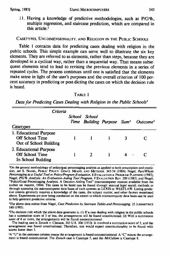
Table 1 contains data for predicting cases dealing with religion in thepublic schools. This simple example can serve well to illustrate the six keyelements. They are referred to as elements, rather than steps, because they aredeveloped in a cyclical way, rather than a sequential way. That means subse-quent elements tend to lead to revising the previous elements in a series ofrepeated cycles. The process continues until one is satisfied that the elementsmake sense in light of the user's purposes and the overall criterion of 100 per-cent accuracy in predicting or post-dicting the cases on which the decision ruleis based.

TABLE 1

Data for Predicting Cases Dealing with Religion in the Public Schools3

CriteriaSchool SchoolTime Building Purpose Sum' Outcome5

Casetypes

1. Educational PurposeOff School Time 1 1 1 3 COut of School Building

2. Educational PurposeOff School Time 1 2 1 4 CIn School Building

'On the general methodology of policy/goal percentaging analysis as applied to both prescription and predic-tion, see S. NAGEL, PUBLIC POLICY: GOALS, MEANS, AND METHODS. 343-54 (1984); Nagel, Part/WholePercentaging as a Useful Tool in Policy/Program Evaluation, 8 EVALUATION & PROGRAM PLANNING (1985);Nagel, P/G% Analysis: An Evaluation-Aiding Tool Program, 9 EVALUATION REV. 209 (1985); and Nagel,"Policy/Goal Percentaging Analysis: A Decision-Aiding Tool" (microcomputer manual available from theauthor on request, 1984). The cases to be listed can be found through manual legal search methods orthrough accessing the microcomputer data bases of such systems as LEXIS or WESTLAW. Listing predic-tive criteria generally requires a knowledge of the cases, the subject matter, and other factors mentionedabove. Experiments are now being conducted on the extent to which microcomputer data bases can be usedto help generate predictive criteria.'The above data comes from Nagel, Case Prediction by Staircase Tables and Percentaging. 25 JURIMETRICS168 (1985).'The decision rule which the above data generates is: (I) If a case dealing with religion in the public schoolshas a summation score of 5 or less, the arrangements will be found constitutional. (2) With a summationscore of 6 or more, the arrangements will be found unconstitutional.

The leading case is Zorach v. Clauson, 343 U.S. 306 (1952). It involved a summation score of 5, and thearrangement was found constitutional. Therefore, one would expect constitutionality to be found withscores lower than 5.'A "U" in the outcome column means the arrangement is found unconstitutional. A "C" means the arrange-ment is found constitutional. The Zorach case is Casetype 7, and the McCullom is Casetype 8.

Spring, 1985]

AKRON LAW REvIEW

TABLE 1 (Continued)

Data for Predicting Cases Dealing with Religion in the Public Schools

CriteriaSchool School

Time Building Purpose Sum OutcomeCasetypes

3. Educational PurposeOn School Time 2 1 1 4 COut of School Building

4. Religious IndoctrinationOff School Time 1 1 2 4 C6

Out of the School Building5. Educational Purpose

On School Time 2 2 1 5 CIn School Building

6. Religious IndoctrinationOff School Time 1 2 2 5 CIn the School Building

7. Religious IndoctrinationOn School Time 2 1 2 5 COut of the School Building

8. Religious IndoctrinationOn School Time 2 2 2 6 UIn the School Building

The cases listed on the rows of Table 1 are not specific cases, except forCase 7 which is Zorach v. Clauson7 , and Case 8 which is McCollum v. Boardof Education'. Instead the "cases" are casetypes formed by combining thecategories on the three predictive criteria. The first predictive criterion iswhether the religious activity was on school time. A "yes" scores 2, and a "no"scores 1. The second predictive criterion is whether the religious activity waswithin the school building, with a yes scoring 2 and a no scoring 1. The thirdcriterion is whether the purpose of the religious activity is for indoctrination(i.e., instilling or strengthening religious beliefs) (scored 2), or is for educationas in a course on comparative literature or cultural geography (scored 1). Ahigh score or a 2 on each predictive criterion indicates a score in the directionof unconstitutionality for these cases. Thus with three predictive criteria, each

'he Outcome of Case 4 is known from the case of McCullom v. Board of Educ., 333 U.S. 203 (1948).

'343 U.S. 306 (1952).

8333 U.S. 203 (1948).

[Vol. 18:4

of which is a yes-no dichotomy, there can be eight casetypes or possible com-binations of the categories. Those casetypes are listed in the first column in theorder of the summation scores for each casetype. Where two casetypes havethe same summation scores, they are listed alphabetically.

After clarifying the cases or casetypes and the predictive criteria, the thirdelement involves showing the relations between each case/casetype and eachpredictive criterion. That is easy here since the definition of each casetypeshows how it is positioned on each criterion. The fourth element involves sum-ming the relation scores in order to obtain an overall score for each case. Thatis also easy here since the raw scores can be summed, because all the predictivecriteria are measured on the same 1-2 scale. We therefore do not have a prob-lem of multi-dimensionality which is present when we try to add apples tooranges, years to dollars, or a 1-2 scale to a 1-5 scale.

The fifth element involves relating the summation scores to the outcomesin the form of a decision rule. Predictive decison rules in this context have theform, "If a case has a summation score of __ or more, then predict a decisionof __ ; and if a case has a summation score of __ or less, then predict an op-posite decision. To aid in developing decision rules, the computer program ar-ranges the casetypes in the order of their summation scores with ties brokenalphabetically. Before the computer calculates the summation scores, it asksthe user for (1) the labels for the casetypes or the names for the specific cases,(2) the labels for the predictive criteria, (3) an indication whether the criteriaare all measured the same way or differently, and (4) the relative importance orweights of the criteria. Here the criteria are weighted equally, meaning theyeach receive a weight of 1. Where differential weights are involved, thoseweights are used to multiply the relation scores in order to work with weightedrelation scores and thus weighted summation scores.

A sixth and especially important piece of information is the outcome foreach case or casetype. That is normally easy information to provide wherespecific cases are involved. Where casetypes are involved as here, deductivereasoning may be needed to indicate the outcomes for those casetypes that donot correspond to specific cases. For example, in Zorach,9 the Supreme Courtupheld religious indoctrination on school time although not in the schoolbuilding. The Court would then surely uphold religious indoctrination not onschool time and not in the school building which is Casetype 4. In other words,if a case wins with an unfavorable score on Criterion A and a favorable scoreon Criterion B, then it is even more likely to win with a favorable score onCriterion A if all other variables are held constant. This is known as afortiorireasoning. One can similarly deduce Casetype 1 where all three variables arefavorable, and Casetype 3 where two variables are favorable rather than justone, and the one unfavorable variable has not changed. Another form of afor-

9343 U.S. 306 (1952).

USING MICROCOMPUTERSSpring, 19851

AKRON LAW REVIEW

tiori reasoning which is not present here is to say if a case loses with afavorable score on Criterion A, then it will lose even more with an unfavorablescore on Criterion A if everything else is held constant.

Likewise, if the Court explicitly says or implies that being on or off schooltime and in or out of the school building are of approximately equal impor-tance, then one can deduce Casetype 2 and Casetype 6 since they interchangethe scores on those two variables as compared to the Zorach0 Casetype 7. Alsoif the Court explicitly says or implies that an educational purpose provides anexemption from unconstitutionality, then we can deduce that Casetype 5 willbe found constitutional, as well as Casetypes 1, 2, and 3. Casetype 8 does nothave to be deduced since it corresponds to the specific case of McCullom v.Board of Education." If that case had not been decided, one would predict un-constitutionality from language that implies being in an unfavorable positionon all three variables, crossing the threshold of unconstitutionality. When theoutcome column has been completed, one should have no trouble seeing thatthe data generates a decision rule saying that if a case has a summation scoreof 6 or more, then predict a decision of unconstitutionality; and if a case has asummation score of 5 or less, then predict a decision of constitutionality.

As an example of sensitivity analysis in this substantive context, onecould add a fourth variable such as whether or not the program is voluntary.We would then have 16 casetypes since we would have four dichotomousvariables which lend themselves to 2 x 2 x 2 x 2 or 16 casetypes. The relationswould still be determined by the definitions of the casetypes. Adding thatfourth variable brings in the concept of violating a constitutional constraint, inthe sense that all eight casetypes where the program is not voluntary would beunconstitutional. In other words, having a compulsory religious program isenough to generate an unconstitutionality decision, regardless of how thecasetype is scored on the other three variables, even if the program is educa-tional rather than doctrinal. A sensitivity analysis, however, is subject tochange when the new inputs actually occur in a future case. Those new casescan then become part of the dataset that is used to develop and revise the deci-sion rules.

SPECIFIC CASES, RESOLVING INCONSISTENCIES, AND LEGISLATIVE REDISTRICTING

A. Analyzing the Specific Cases

Table 2 contains data for predicting legislative redistricting cases. Thecases listed on the rows are all specific cases, rather than casetypes. They are

'od.

"333 U.S. 203 11948).

'2Cases dealing with religion in the public schools are discussed in N. DORSEN, P. BENDER, & B. NEUBOINE.POLITICAL AND CIVIL RIGHTS IN THE UNITED STATES, (1976), [hereinafter cited as N. DORSENJI, H. PRITCH-ETr, CONSTITUTIONAL CIVIL LIBERTIES 150-54 (1984). For further details on predicting civil liberties casesquantitatively, see Nagel, Predicting Court Cases Quantitively, 63 MICH. L. REV. 1411 (1965).

[Vol. 18:4

USING MICROCOMPUTERS

the most important legislative redistricting cases decided in the United Statesby various courts from Colegrove v. Green,3 through Baker v. Carr'. Thecases are arranged in the order of their summation scores. That happens to beroughly the same as the chronological order of the cases, which shows that thecases became more favorable toward ordering redistricting as one moved fromColegrove to Baker.

TABLE 2

Data for Predicting Redistricting Cases 5

Criteria'7

Equality State Equality Federal Sum" OutcomeRequirement Legislature Violation Court

Casetypes"s1. Colegrove9 1 1 1 2 5 D2. Grills'° 2 2 1 1 6 A3. Maryland2 1 2 2 1 6 D4. Schollen 1 2 2 1 6 D5. WMCA 23 1 2 1 2 6 D6. Asbury 4 2 2 2 1 7 A7. Dyer25 2 1 2 2 7 A8. Baker26 2 2 2 2 8 A9. Magraw27 2 2 2 2 8 A

3328 U.S. 549 (1946).14369 U.S. 186 (1962).

"5The above date comes from Nagel, Applying Correlation Analysis to Case Prediction, 42 TEx. L. REV.1006-17 (1964).

"The decision rule which the above data generates is: (1) If a redistricting case during the time periodcovered has a summation score of 7 or above, the attacker wins. (2) With a summation score of 6 or below,the defender wins. That decision rule generates one inconsistent case. The inconsistency can be eliminatedby: (1) Changing the decision rule to say a summation score of 6 leads to an unclear outcome. (2) Giving thefirst variable a weight of 2, which would be consistent with the importance of requiring equality. (3) Addinga fifth variable called "Decided After the Maryland Case." (4) Eliminating the Grills case, but that does notseem justifiable. (5) Changing the measurement on the first variable from no-yes to a 1-3 scale and givingGrills a score of 3. (6) Finding that Grills really deserves a 2 on the third or fourth variables.

"A one in columns one through four equals no. A two in columns one through four equals yes. An "A" inthe outcome column means the attacker wins. A "D" means the defender wins.

" When working with cases, rather than casetypes, inconsistencies are likely to occur that need resolving.

'gColegrove v. Green, 328 U.S. 549 (1946).

"Grills v. Anderson, 29 U.S.L.W. 2443 (Ind. 1961).2 Maryland Comm. for Fair Representation v. Towes, 377 U.S. 656 (1964).

"Scholle v. Hare, 360 Mich. I, 104 N.W.2d 63 (1960), vacated, 369 U.S. 429 (1962) reh'g denied, 370 U.S.906 (1962), on remand, 367 Mich. 176, 116 N.W.2d 350 (1962), cert denied, Beadle v. Scholle, 377 U.S. 990(1964).

'3W.M.C.A., Inc. v. Simon, 196 F. Supp. 758 (S.D.N.Y. 1961).

"Asbury Park Press v. Woolley, 33 N.J. 1, 161 A.2d 705 (1960).

"Dyer v. Abe, 138 F. Supp. 220 (D. Hawaii, 1956).

'Baker v. Carr, 369 U.S. 186 (1962).

"Magraw v. Donovan, 163 F. Supp. 184 (D. Minn. 1958).

Spring, 19851

AKRON LAW REVIEW

There are four predictive criteria. As with the cases dealing with religionin the public schools, all four criteria are measured using a yes-no dichotomy.The first variable asks whether the relevant constitution expressly requiresdistricts of equal population per representative. The Colegrove case, for exam-ple, involved Congressional redistricting.28 The federal Constitution does notexpressly require equality.29 On the contrary, it expressly requires that eachstate have at least one representative, no matter how small the state might be?0

Equality for Congressional districting has been read into the federal Constitu-tion by way of finding it implicit in the due process clause of the fifth amend-ment and the equal protection clause of the fourteenth amendment. The Bakercase, on the other hand, involved Tennessee state legislative-redistricting.31

The Tennessee Constitution does explicitly require equality, which had beenignored for years by the refusal of the state legislature to redistrict.32

The second variable asks whether a state or federal legislature is involved.A state legislature is scored 2, and the federal legislature is scored 1. Statelegislatures are more likely to be ordered to redistrict because the courts (atleast in those early years) seemed to show more respect for not upsetting Con-gress. Oliver Wendell Holmes had said the federal system could survive if Con-gress violated the Constitution, but not if the states did so. The third variablerefers to the degree of equality violation. If less than 35% of the state's popula-tion can choose more than 50% of the state legislature, then the equality viola-tion is high (scored 2). If more than 35% of the state's population is required tochoose more than 50% of the state legislature, then the equality violation isrelatively low (scored 1). The fourth variable asks whether a federal or statecourt is deciding the case. One would expect a federal court to be more likely todecide in favor of redistricting in view of the lifetime appointment of federaljudges, which makes them less susceptible to pressure from the dominantpolitical party.

With nine cases and four predictive criteria, there are 36 relations. Theyare shown in the cells of Table 2. Those relation scores can be objectivelydetermined, as are the relation scores in most court case prediction. The fourthkey element in the predictive analysis involves summing the relation scores foreach case and arranging the cases in the order of their summation scores. Theminimum summation score is 4 for a case that scores I on all four variables.There was no such case which is a further indication that we are dealing withactual cases, rather than casetypes. The Colegrove case comes closest with ascore of 5. The maximum score possible is 8 for a case that scores 2 on all fourvariables. Baker is an example of that casetype.

-328 U.S. 549 (1946).

"Id. at 551.

"Id. at 556.3-369 U.S. 186 (1962).

'Md. at 207-08.

[Vol. 18:4

USING MICROCOMPUTERS

With actual specific cases, the prior outcomes are generally easy to deter-mine. Of these nine cases, five were decided in favor of the party attacking theexisting apportionment, and four in favor of the party defending it. The deci-sion rule which the data generates is that if a redistricting case during the timeperiod covered has a summation score of 7 or above, the attacker wins. With asummation score of 6 or below, the defender wins. That decision rule, how-ever, results in at least one inconsistency. This is so because four cases receivedscores of 6 apiece, and one of the four resulted in a victory for the attackerwhen the other three were won by the defender of the existing redistricting.

B. Resolving the Inconsistencies

The P/G% system provides methods whereby the system can guarantee100% accuracy in predicting the past cases on which the decision rule is based.This is the equivalent in statistical regression analysis of guaranteeing therewill be no residuals or differences between predicted scores and actual scoreswhere one is predicting winning or losing. It is possible that there are some realinconsistencies across cases, judges, places, or time periods. The philosophy ofthe P/G% approach, however, assumes that the inconsistencies are only on thesurface, and that if one does a better analysis of the cases, criteria, relations,weights, measures, and other inputs, then the inconsistencies will disappear.The P/G% approach facilitates such an analysis by enabling the user to easilydetermine the effects of changes in those inputs and by allowing for variablesthat refer to when, where, and by whom the cases were decided.

There are at least six ways of resolving what otherwise would be inconsis-tencies or residuals. Taking them in random order as applied to Table 2, onecan change the decision rule to say a summation score of 7 or above leads tothe attacker winning; a summation score of 5 or below leads to the defenderwinning; and a summation score of 6 leads to an unclear result. There wouldthen be no inconsistencies since a summation score of 6 could then accommo-date both an A and a D for its outcome. That approach, is, however, unde-sirable, because it may declare too many cases to be unpredictable. In this ex-ample, an undesirable four out of the nine cases would become unpredictable.

A more meaningful approach is to give the first criterion a weight of 2.That would have the effect of doubling all the numbers in that column beforethe summing is done. Doing so would mean the new summation scores wouldbe 6, 8, 7, 7, 7, 9, 9, 10, and 10 respectively. The new decision rule would thenbe that a summation score of 8 or above leads to a redistricting order and asummation score of 7 or below leads to such an order being denied. In otherwords, each case that scored 1 on the equality requirement would move up oneextra point on the summation score, and each case that scored 2 on the equali-ty requirement would move up two extra points on the summation score. That

Spring, 19851

[Vol. 18:4AKRON LAW REVIEW

means the Grills33 case would move up from a 6 to an 8, and the other threecases that started at 6 would move up to a 7, because only Grills of the fourcases received a 2 on the equality requirement. Giving the requirement ofequality a weight of 2 when the other criteria receive a weight of 1 is substan-tively reasonable, since whether equality is required should be especially fun-damental in determining whether a redistricting is ordered for lack of equality.The other criteria are less fundamental in that sense.

Instead of or in addition to changing the weights of the criteria, one couldadd an additional criterion. For example, the inconsistency would be resolvedif we added a time variable which asks whether the case was decided after theMaryland case.34 There were only two cases decided after the Maryland case,namely Grills" and Baker.36 Thus they would be the only cases receiving a 2 onthis new variable. All the others would receive a 1. That would mean the newset of nine summation scores would be 6, 8, 7, 7, 7, 8, 8, 9, and 8. Unlike thedifferential weighting, however, adding that variable is not so substantivelyreasonable. That time point was not a watershed in any sense, but rather justan arbitrary way of separating Grills from the other three cases. That timevariable would have been more meaningful if there had been years rather thanmonths separating the Maryland case from the Grills case, or if the Marylandcase had established an important new precedent favoring redistricting whichwas applicable to Grills.

Another alternative might be to eliminate the Grills case. That does

eliminate the inconsistency. It would be justifiable if the Grills case really didnot belong by virtue of its being a foreign redistricting case, a redistricting of

fire stations rather than legislative districts, or some other substantively mean-

ingful reason. There is no such reason here. Any approach to eliminate incon-

sistencies must also be substantively meaningful. Approaches which do not

work with Table 2 might, however, work with other sets of cases.

Another approach is to change the measurement on one or more predic-

tive criteria. For example, perhaps the requirement of equality could be

measured in three categories, rather than just yes-no. The three categoriesmight be strongly yes, mildly yes, and no. If the constitution in the Grills casestrongly requires equality, then that case would receive a 3 on the firstvariable, and the other three cases would remain at 1. The new summationscores would then be 7, 6, 6, and 6 for those four cases, which would separateGrills from the other three cases without creating any new inconsistencies.Another example might involve noting that the equality violation is rathercrudely measured with a yes-no dichotomy. A more sophisticated measure-

33Grills v. Anderson, 29 U.S.L.W. 2443 (Ind. 1961).

-377 U.S. 656 (1964).

1129 U.S.L.W. 2443 (Ind. 1961).

"'369 U.S. 186 (1962).

USING MICROCOMPUTERS

ment might ask what is the minimum percentage of the population needed toelect 51 % of the legislature. The answer could range from a low of about 10%to a high of 51 %. The Grills case, however, would not receive a substantiallyhigher score on the degree of equality violation than those other three cases,since it received a no on the yes-no dichotomy when two of the other threereceived a yes.

Another alternative relates to finding an error in how the cases have beenscored on each criterion. If, for example, Grills really deserves a 2 on the thirdor fourth variables, then the inconsistency would be resolved. That approach ismore likely where there is more subjectivity in scoring the relations. An errorcould also occur in calculating the summation scores if they were calculated byhand or with a calculator. The microcomputer, however, is not likely to err insumming the relation scores even if they are multi-dimensional and weighted.The program also shows intermediate values between the raw scores and thesummation scores to enable the user to check that the summation was doneproperly. The intermediate scores show the corresponding part/whole percen-tages for each raw score to consider multi-dimensionality (which will bediscussed shortly), and weighted raw scores or weighted part/whole percentagescores to consider differential weighting.

All these changes are directed toward improving predictive decision rulesby (1) having them make more substantive sense and by (2) reducing incon-sistencies. The changes can be summarized in the form of a checklist in whicheach item refers to an input element that is subject to change as follows:

1. Cases or Casetypes(1) Adding or subtracting(2) Consolidating or subdividing(3) Specifying a maximum or minimum on a characteristic of a

casetype

2. Predictive Criteria(1) Adding or subtracting(2) Consolidating or subdividing(3) Specifying a maximum or a minimum on a predictive criterion

3. Relations between Cases and Criteria(1) More refined or less refined measurement(2) Alternative units of measurement(3) Different scoring for some of the relations

Spring, 1985]

AKRON LAW REVIEW

4. Drawing a Conclusion as to the Predictive Decision-Rule(1) Expanding or contracting the indeterminate area(2) Changing the upper or lower cut-off(3) Predicting degrees, rather than a dichotomy or vice versa(4) Predicting degrees with a non-linear, rather than a linear equation

or a different kind of non-linear equation(5) Recognizing a constraint such that if it is present, all cases will be

decided positively, or all cases will be decided negatively, regardlesshow they score on the predictive criteria.

C. Sensitivity Threshold Analysis

The computer program aids the user in determining which alternative isbest for eliminating inconsistencies. The program does so in various ways. Oneway is to inform the user what it would take to move the Grills case up to a tiewith the lowest scoring case in which the attacker won. That kind of thresholdanalysis shows how each of the four relation scores or their weights wouldhave to change. Another way is to inform the user what it would take to movethe other three cases down to a tie with the highest scoring case beneath themin which the defender won. Probably the best way in which the sensitivityaspects of the program are helpful here is by enabling one to experiment quick-ly and accurately with different weights, variables, sets of cases, measurementunits, and relation scores to see what their effects are in terms of new summa-tion scores and the elimination of previous inconsistencies without introducingnew ones.

A special form of sensitivity or threshold analysis in this substantive con-text could involve asking what would have enabled Colegrove to be decided infavor of the attacker the way Baker was. The answer is that it would havetaken a combination of changes great enough to make up the 3-point gap be-tween the score of 5 which Colegrove received and the score of 8 for Baker.The gap could be made up if Colegrove could receive a score of 4 on the equali-ty requirement or Baker a score of -1. Neither change, however, is possiblesince that criterion only provides for scores of 1 and 2. The same thing is trueof all the other criteria in that no change on any of them is possible that willmake up the 3-point gap. The threshold analysis also informs us that the gapcould be made up if any one of the first three criterion were to be given aweight of -2. Then Colegrove would receive weighted relation scores of-2+ I + 1 +2 which sum to +2, and Baker would receive scores of-4 + 2 + 2 + 2 adding to + 2 just like Colegrove. A -2 weight, however, makesno substantive sense for any of the first three variables. No weight will helpColegrove for the fourth variable. Both Colegrove and Baker receive the sameraw score on that variable, since they were both decided in federal courts.

[Vol. 18:4

TABLE 3

An Example of the Computer Display: Threshold Analysis37

Threshold Analysis Colegrove vs BakerEq. Requ Legis. S Eq. Viol Court Fe

Coleg 4.00 4.00 4.00 5.00Baker -1.00 -1.00 -1.00 -1.00Weight -2.000 -2.000 -2.000 ????

The threshold analysis is summarized in Table 3. The first row indicatesthe threshold values for the Colegrove case on each of the four variables. Thesecond row indicates the threshold values for the Baker case. The third row in-dicates the threshold weights for each of the four predictive criteria. Thisanalysis informs us that it would have been virtually impossible for Colegroveto have been decided any other way in view of the validity and meaning ofthese predictive variables, plus other variables that also disfavored Colegrove.

To apply the decision rule of Table 2, one needs a new case that is not in-cluded in the data set from which the decision rule was generated. If the nextcase after Baker involves no equality requirement, a state legislature, a severeequality violation, and a federal court, then the case would have 7 unweightedpoints. We would then predict victory for the attacker, since 6.5 is the cutoffsummation score. If we weight the equality requirement by 2, then the newcase would have a weighted summation score of 8. We would still predict vic-tory, since the cutoff score with the weights is 7.5. We could test the predictivepower of the methodology by predicting Case 3 from the first two, Case 4 fromthe first three, and so on. If we do that, we will predict accurately each time,provided that we use the weighting system whereby scores on the equality re-quirement are doubled, while the other scores remain unchanged.38

"The object here is to determine what it would take to bring Colegrove up to the same summation score as

Baker, or to bring Baker down to the same summation score as Colegrove.Each cell shows the threshold value of a relation or a weight. If an actual cell value in Table I were to

change to its above threshold value, then there would be a tie between Colegrove and Baker, assuming all

the other inputs are held constant.No one threshold value can equalize Colegrove and Baker given the four criteria. All the threshold values

are above or below the measurement range of 1-2. There is also no substantive sense for the weights of any

of those predictive variables to be negative rather than positive.3 The cases dealing with legislative redistricting are discussed in R. DIXON, DEMOCRATIC REPRESENTATION:

REAPPORTIONMENT IN LAW AND POLITICS (1968) and REAPPORTIONMENT IN THE 1970's (Polsby ed., 1971).For further detail on this predictive example, see Nagel, Applying Correlation Analysis to Case Prediction.

42 TEX. L. REV. 1006 (1964). Other variables that also disfavored Colegrove include (1) the intervening case

of Gomillion v. Lightfoot, 364 U.S. 339 (1960), which ordered redistricting where blacks were being

districted out of the city limits of Tuskegge, Alabama, (2) the partial reliance in the Colegrove case on the

clause that guarantees a republican form of government, rather than the equal protection clause, (3) the in-

creased public sensitivity to denials of equality between 1946 and 1962, (4) the increased malapportionment

between 1946 and 1962, especially as a result of increased urban and suburban growth with virtually no new

redistricting, and (5) the request in Colegrove for redistricting in time for the next congressional election

which was only a few months away. The threshold weight of -2 is calculated by the computer by solving for

USING MICROCOMPUTERSSpring, 19851

AKRON LAW REVIEW

MULTI-DIMENSIONALITY AND HOUSING DISCRIMINATION CASES

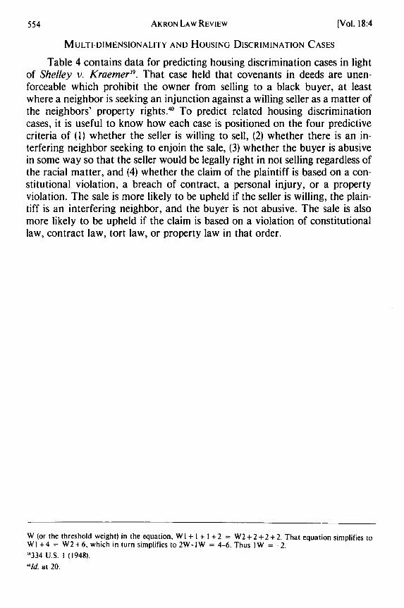
Table 4 contains data for predicting housing discrimination cases in lightof Shelley v. Kraemer 9. That case held that covenants in deeds are unen-forceable which prohibit the owner from selling to a black buyer, at leastwhere a neighbor is seeking an injunction against a willing seller as a matter ofthe neighbors' property rightsi ° To predict related housing discriminationcases, it is useful to know how each case is positioned on the four predictivecriteria of (1) whether the seller is willing to sell, (2) whether there is an in-terfering neighbor seeking to enjoin the sale, (3) whether the buyer is abusivein some way so that the seller would be legally right in not selling regardless ofthe racial matter, and (4) whether the claim of the plaintiff is based on a con-stitutional violation, a breach of contract, a personal injury, or a propertyviolation. The sale is more likely to be upheld if the seller is willing, the plain-tiff is an interfering neighbor, and the buyer is not abusive. The sale is alsomore likely to be upheld if the claim is based on a violation of constitutionallaw, contract law, tort law, or property law in that order.

W (or the threshold weight) in the equation, W I + I + I + 2 = W2 + 2 + 2 + 2. That equation simplifies to

WI +4 = W2+6, which in turn simplifies to 2W-IW = 4-6. Thus IW = -2.

"9334 U.S. 1 (1948).

Id. at 20.

[Vol. 18:4

Spring, 1985]

• - -

V

;5

USING MICROCOMPUTERS

'.0 -; '.0 c "r a,, 1cC cn cl) .~. I-z

00 In 00 el r- cC4 1--q fN- m- m- -

C-. c - C-* c.

C-C CC ~ ~C rC ~ '.0c-

- -I cn -d - "-- m ~. 0c--a

00 00 00 r- c - rL- -

. - C14 " '- C-4 1- c

"D 0 -E EC- C- €"- a ..

E%. E 2'L - E~ E m 2-5~~~~ E (u -'m.'z E 'rO 2

C0

C* 0 C 0- 3 )15(

.- c._ .C "5 n '. r- 00

w bo

1~0

o E~

~E

E >u

E .

iorUr

< Z

2., 0

0' .E

< cc

AKRON LAW REVIEW

To illustrate the problem of multi-dimensionality in predictive criteria,Table 4 only uses criteria 1 and 4 which relate to the willingness of the sellerand the nature of the claim. The multi-dimensionality problem involves thefact that the willingness of the seller is measured in terms of a yes-nodichotomy, whereas the nature of the claim is measured in terms of fourcategories. With two categories on one criterion and four on the other, thereare eight casetypes, as listed at the left of Table 4. Column 1 shows how theeight casetypes score on the willingness variable, and column 3 shows howthey score on the claim variable. Column 5 adds those raw relation-scorestogether to obtain an unweighted raw sum. Column 6 shows that the sale willbe allowed if the seller is willing. If the seller is unwilling, the outcome dependspartly on the other variables which are not included in Table 4.

Where the predictive variables are measured differently, merely summingthe raw scores produces distorted results. That would be more obvious if onepredictive criterion were measured in miles, and a second predictive criterionwere measured in pounds. The results are also distorted if a case receives 4points for being in the best category on the claim variable, while a case receivesonly 2 points for being in the best category on the willingness variable. That isdue to the coincidence that the claim variable has four categories, and the will-ingness variable has only two categories. Partly to remedy that situation, therelation scores are transformed into part/whole percentages which are not in-fluenced by whether a variable is measured in miles, pounds, a yes-nodichotomy, or a 1-4 scale.

To transform the relation scores on a given criterion or column, one mere-ly sums the numbers in the column to obtain a total or whole. For example,the sum of the first column is 12. One then divides each number or part in thecolumn by the whole in order to obtain a part/whole percentage for each rela-tion score. For example, the part/whole percentage corresponding to the firstrelation score in column 1 is 1/12 or 8%. Now instead of adding the raw scoresof column 1 to those of column 3 in order to obtain the unweighted raw sum ofcolumn 5, one adds the part/whole percentages of column 2 to the part/wholepercentages of column 4 to obtain the sum of the unweighted part/wholepercentages of column 7. For example, adding 8% in column 2 to 5% in col-umn 3 gives 13% in column 7.

Notice that by working with just the unweighted raw sum there are threeinconsistencies out of eight cases. The three inconsistencies are cases 2, 3, and4. They have unweighted sums that are as high as cases 5, 6, and 7. Cases 2, 3,and 4, however, have unclear outcomes, whereas cases 5, 6, and 7 resulted in

[Vol. 18:4

USING MICROCOMPUTERS

the sale being allowed. By working with the sum of the unweighted part/wholepercentages, there are only two inconsistencies. They are cases 3 and 4. Theyhave unweighted part/whole percentages larger than cases 5 and 6. Cases 3 and4, however, have unclear outcomes, whereas cases 5 and 6 resulted in the salebeing allowed. All the inconsistencies can be eliminated by recognizing thatthe willingness of the seller is more important than the nature of the claim. Ifwillingness is given a weight of 2, then the sum of the weighted p/w%'s for thefirst casetype is twice 8% plus 5% for a total of 21 %. If one does likewise foreach of the eight casetypes, one obtains the sums of weighted p/w%'s shown incolumn 8. The percents in that column are in perfect ascending order, suchthat there are no inconsistencies. If a casetype has a sum of weighted p/w%'sof .39 or higher, then the willing seller wins and the sale is allowed. If acasetype has a sum of weighted p/w%'s of .36 or lower, then the unwillingseller may be allowed to get out of the sale depending on whether or not thebuyer is abusive."

OUTCOME RANGES AND INTERNATIONAL LAW CASES

Table 5 contains data for predicting international law cases where theUnited States is a party. The object is to predict the probability that the UnitedStates will win from at least two predictive criteria. The predictive criteria arethe source of law and the industrial power of the U.S. opponent. They are twocriteria from a larger list of seven, which also includes (1) the international lawsubject matter and the U.S. position on it, (2) the decision-making tribunal, (3)the economic interests that may be involved and the U.S. position on them, (4)the civil liberty interests that may be involved and the U.S. position on them,and (5) the nature of the plaintiff as a legal entity.

"Cases dealing with housing discrimination are discussed in J. KUSHNER. FAIR HOUSING: DISCRIMINATION INREAL ESTATE. COMMUNITY DEVELOPMENT AND REVITALIZATION (1983); R. SCHWEMM. HOUSINGDISCRIMINATION LAW (1983), and N DORSEN. supra note 12, at 940-46. For further details on this predictiveexample, see Nagel, Case Prediction by Staircase Tables and Percentaging, 25 JURIMETRICS 168 (1985).

Spring, 1985]

TABLE 5

Data for Predicting International Law Cases with the US. as a Party45

CriteriaSource of Law U.S. Opponent Sum' Outcome"7

Casetypes1. Foreign Law and

Less Industrial Opponent 1 1 2 40%2. Foreign Law and

Non-Country Opponent 1 2 3 483. Treaty and

Less Industrial Opponent 2 1 3 514. Foreign Law and

Equal Opponent 1 3 4 625. International Law and

Less Industrial Opponent 3 1 4 566. Treaty and

Non-Country Opponent 2 2 4 587. International Law and

Non-Country Opponent 3 2 5 638. Treaty and

Equal Opponent 2 3 5 739. U.S. Law and

Less Industrial Opponent 4 1 5 7010. International Law and

Equal Opponent 3 3 6 7811. U.S. Law and

Non-Country Opponent 4 2 6 7812. U.S. Law and

Equal Opponent 4 3 7 925Table 5 only deals with two of the seven variables in the international law cases. The two are the main

source of law and the industrial power of the United States opponent. The source of law includes UnitedStates law, international law, a treaty, and foreign law. The United States opponent can be equal to theUnited States, not a country, or less than the United States in industrial power. Only two variables are usedin Table 4 rather than seven, partly because of the temporary limitation to 15 alternatives. One can handleall seven variables through multiple runs with 15 casetypes per run. The number of casetypes, however, is163,800 since the number of categories per variable of 4, 13, 6, 5, 5, 3, and 7 respectively. Under those cir-cumstances, one would not want to list all the casetypes. Instead, one would want to know what the proba-bility of United States victory is for any combination of seven categories. To estimate that, simply averagethe seven probabilities of United States victory. The above data comes from Nagel, Judicial PredictionAnalysis from Empirical Probability Tables, 41 IND. L. J. 403-19 (1966).

4The decision rule which the above data generates is Y = .20 + . 10(x), where Y is the probability of theUnited States winning and X is the summation score. The decision rule could also be expressed as a series ofif-then statements like (1) if X is 1, then Y is .30; (2) If X is 2, Y is .40; (3) If X is 3, Y is .50; (4) If X is 4, Y is.60; (5) If X is 5, Y is .70; (6) If X is 6, Y is .80; and (7) If X is 7, Y is .90. The above prediction equationcomes from observing the relation between the summation scores and the outcome probabilities in Table 5.One can determine the prediction equation more accurately by using a statistical calculation that can easilyarrive at such an equation for 12 pairs of inputs. One can also think in terms of six pairs of input for the sum-mation scores from 2 to 7. Thus a score of 4 had an average outcome of .57 since Casetype 6 had an outcomeof .56 and Casetype 8 had an outcome of .58.

"The outcome figures shown above come from averaging the two probabilities from the two variables usedfor each casetype. Thus, the combination of United States law and equal power has a .92 probability because

AKRON LAW REVIEW [Vol. 18:4

USING MICROCOMPUTERS

The source of the law refers to the four categories of (1) domestic law ofanother country (the U.S. is victorious in only 25% of such cases), (2) an inter-national treaty (47% victorious), (3) international law/custom (56%), and (4)U.S. domestic law (85%). The industrial power of the U.S. opponent refers tothe three categories of (1) less industrial power than the U.S. (the U.S. is vic-torious in only 56% of such cases), (2) non-countries (70% victorious), and (3)about the same in industrial power (100% victorious although that sub-sampleis small). The victory probabilities are based on an analysis of the 137 casescontained in four leading international law casebooks.

With four categories on one criterion and three categories on the secondcriterion, there are 12 casetypes, as shown at the left side of Table 5. The sum-mation column sums the raw scores for each casetype across the variables.Technically speaking, part/whole percentages should be used since the predic-tive variables are measured differently via a 1-4 scale and a 1-3 scale. Thescales, however, are close enough to justify working with raw scores at leastfor this methodological illustration.

Each probability in the outcome column is arrived at by averaging theprobabilities for the relevant categories on each predictive variable. Thus,Casetype 1 involves foreign law (25% U.S. victory rate) and a less industrialU.S. opponent (56% U.S. victory rate). The average between 25% and 56% is40% rounded to the nearest even number. There are more sophisticated waysof combining probabilities in accordance with Bayesian probability analysis.They are, however, highly complicated, especially when more than two predic-tive variables are involved. The information for a Bayesian analysis is almostnever available since it requires knowing various details on how the predictivevariables relate to each other. Simply averaging the basic probabilities shouldprovide a sufficient approximation to an overall probability, especially if eachpredictive criterion is worded in the direction of winning and does not greatlyoverlap the other criteria. Even if the criteria do overlap, the weights can takethat into consideration. Two duplicative criteria, for example, can each begiven about half the weight they would otherwise receive if the other criterionin the pair were not also being used.

After determining the criteria, casetypes, relations, summation scores,and outcomes, one should develop a decision rule indicating for various sum-mation scores what outcomes are likely to occur. This example, however, dif-fers from the previous examples in that the outcome is a range between 40%and 92% rather than just a dichotomy of winning versus losing. Having an

United States law has a .85 probability and equal power has a 1.00 probability. This gives an approximationto a Bayesian conditional, especially where we only have the main probabilities with which to work. Table 5provides a good illustration of an outcome that is not a dichotomy of win or lose but rather a continuumoutcome of 0 to 1.00.

Spring, 1985]

AKRON LAW REVIEW

outcome range is common in most court cases as well as a win-lose dichotomy.In damage cases, the dichotomous liability-decision is followed by a continuumdamages-decision when liability is established. Damages can range from a lowof $1 in some libel cases to millions of dollars in treble damage antitrust suits.In criminal cases, the conviction decision is followed by a sentencing decisionwhen there is a conviction. Sentences can range from a low of no jail time to

life imprisonment or the death penalty.

In Tables 1 through 5, one could bypass the summation score and for-

mulate a decision rule that specifies for each casetype or case what the out-

come is likely to be. That approach is likely to lead to inconsistencies, as was

shown with the redistricting cases and the housing discrimination cases. It is

also much more clumsy to have to specify how each case or casetype will be

decided, especially if there are many casetypes. With a win-lose dichotomy, the

decision rule simply specifies what summation score separates the winners

from the losers. In predicting a range outcome, there is no such threshold sum-

mation score. Instead, one would like to know the likely outcome at a base

summation score of 0 or 1, and how much the outcome is likely to increase for

each 1-unit increase or 1% increase in the summation score.

Looking at the last two columns of Table 5 tends to generate a decisionrule that Y = .20 + .10(X), where Y is the probability of the U.S. winning,and X is the summation score. One can see that the two casetypes with sum-mation scores of 3 average about a .50 probability; the three casetypes thatscore 4, average about .60; and the three casetypes that score 5 average about.70. Extending those relations downward implies or extrapolates that a sum-mation score of zero would have a probability of about .20. One cannot,however, score less than a 2 on the two predictive criteria together. At theother end, that eyeballing approach implies that a summation score of 8 wouldhave a probability of about 1.00. One cannot, however, score more than 7 onthe predictive criteria. Thus, the eyeballed or linear relation is not subject tothe criticism that it leads to probabilities below zero or above 1.00 since all thepossible summation scores lead to reasonable probabilities when using the deci-sion rule Y = .20 + .10(X).

Greater precision may sometimes be required than the eyeballing ap-proach provides. Under those circumstances, one can insert into a statisticalcalculator the 12 pairs of numbers, consisting of 2 and .40, 3 and .48, and soon. After keying in those 24 numbers, one can read out the value of the con-stant which is. 19 rather than .20, and the value of the slope which is slightlymore than. 10. The computer program will do that kind of statistical regressionanalysis directly when the PIG% program is further developed.

[Vol. 18:4

USING MICROCOMPUTERS

One can also obtain a decision rule which reflects diminishing returns ofthe form Y = .24(X)65 by inserting the same 24 numbers and asking fordiminishing returns output. With that equation, a summation score of 1predicts a probability of .24, and a summation score of 2 predicts a probabilityof .38. Each successive increment on the summation score increases the prob-ability, but at a diminishing rate. The .65 means that if the summation scoredoubles (i.e., increases by 100%), then the probability will increase by about65%. For example if the summation scores doubles from 1 to 2, then thepredicted probability goes up from .24 to .38. The .14 difference is about 65%of the .24 base. Diminishing returns is a fact of life in the relation betweenmost inputs and most outputs, but linear relations often give good enoughpredictability. With the aid of the microcomputer program, one can requesthow one wants the summation scores related to the range outcomes with equalease, regardless whether one chooses constant returns, diminishing returns, orother available options.48

MULTIPLE WEIGHTS FOR PREDICTIVE CRITERIA AND CRIMINAL CASES

Table 6 contains data for predicting criminal cases. The data is purelyhypothetical, unlike any of the previous five tables. For methodological pur-poses, however, hypothetical data should be just as usable as real data. Thisdata is not only hypothetical, it is also symbolic data, meaning the cases andcriteria only have letters not names. The advantage of such data is that itenables one to see the methodology more clearly without substance getting inthe way. Another advantage is that this particular set of hypothetical data isthe first court-case prediction problem with which this author dealt back in1960. This example thus illustrates some important changes over the past 25years in systematic quantitative judicial prediction.

'The international law casebooks which provide the data base for this example are W. BISHOP. INTERNA-

TIONAL LAW (1953); M. HUDSON, INTERNATIONAL LAW (1951); M. KATZ& K. BREWSTER, INTERNATIONALTRANSACTIONS & RELATIONS (1960); L. ORFIELD & E. RE, INTERNATIONAL LAW (1955). For further details onthis predictive example, see Nagel, Judicial Prediction and Analysis from Empirical Probability Tables, 41IND. L.J. 403 (1966). Working with probabilities of victory and average damages under various circum-stances can be facilitated by such loose-leaf services as those published by the Jury Verdict Research Service.

Spring, 19851

TABLE 6

Data for Predicting Hypothetical Criminal Cases9

Criteria"P Criterion Q Criterion R Criterion S Criterion Unweighted Weighted(W= +.75) (W= -. 67) (W= + 1.00) (W= +.67) Sum Outcome5 Sum52

Casetypes

1. A 1 2 1 1 5 P 1.09

2. C 2 2 1 1 6 P 2.09

3. B 2 2 2 2 8 D 3.50

4. D 2 1 2 1 6 D 3.50

5. E 2 i 2 2 7 D 4.16

There are five criminal cases called A, B, C, D, and E, although the data isgeneral enough to be any kind of case. There are four predictive criteria calledP, Q, R, and S. There are thus 20 relations. Each relation is a yes-no di-chotomy. The criteria are worded in such a way that a yes answer favors thedefense, and a no answer favors the prosecution. If one adds the unweightedraw relation scores across each case, one obtains unweighted sums of 5, 8, 6, 6,and 7 for cases A, B, C, D, and E, respectively. Those raw scores generate oneinconsistency out of five opportunities, since both case C and D have 6 points,but C was decided in favor of the prosecution and D in the favor of thedefense.

The best way to eliminate inconsistencies is generally by giving the predic-tive criteria different weights, rather than having the same weight for all thecriteria. The best way to determine those weights is generally in terms of therelative substantive importance of the variables as known to reasonablyknowledgeable people. That is what was once done (1) in the cases dealing withreligion in the public schools, in saying educational purpose is an exemptionvariable and compulsory participation is a constraint variable, (2) in theredistricting cases, in saying the presence of an equality requirement is more

"The above data comes from Nagel, Using Simple Calculations to Predict Judicial Decisions, 7 PRAC. LAW.68-74 (1961)."There are various ways in which one can assign weights to predictive criteria. The method used here is todetermine the correlation coefficient of each predictive variable with whether the prosecution or defendantwins. In other words, outcome can be considered a dichotomous Y variable to be correlated with the X I, X2,X3, and X4 predictive criteria.

This is a good example of the use of weights for the predictive variables."A "P" in the outcome column means the prosecution wins. A "D" means the defense wins."The decision rule which the above data generates is: (I) If the weighted summation score is 3.50 or above,the defendant wins. (2) With a summation score of 2.09 or below, the prosecution wins. (3) If the weightedsummation score is between 2.09 and 3.50 the result is unclear. The weighted summation scores arecalculated by multiplying the raw scores on each predictive criterion by the weight of the criterion. Thoseproducts are then added across each case. There is one inconsistency with the unweighted summationscores, but no inconsistencies with the weighted summation scores.

AKRON LAW REVIEW [Vol. 18:4

important than the other variables, and (3) in the housing discrimination cases,in saying the willingness of the seller is more important than the field of law.The best tests of how well the cases have been weighted are whether theweighting makes substantive sense, and whether the weighting results in aperfect separation of the winning cases from the losing cases.

An alternative weighting method is to weight the criteria in terms of theirassociation with the outcome that one is trying to predict. That is what is donein Table 7. That table shows how the weights for Table 6 were determined. Forexample, criterion P has a weight of + .75 because 75% of the cases that had Ppresent resulted in victory for the defense, whereas 0% of the cases that had Pabsent resulted in victory for the defense. By subtracting those two percen-tages, one obtains a constant of zero and a slope of .75 in an equation of theform Y = 0 + .75(X). Y is the case outcome (with 0 for P and 1 for D), and Xis the general predictive criterion (with 0 for absent and 1 for present). Thus ifthe predictive criterion moves from 0 to 1, the outcome then moves from aprobability of 0% for the defense winning on up to 75%. The other four sub-tables of Table 7 can be interpreted the same way to yield equations of theform Y = 1.00 - .67(Q); Y = 0 + 1.00(R); and Y = .33 + .67(S).

TABLE 7

Weighting Predictive Criteria by Association with Outcome53

P Criterion Q Criterion

No Yes No Yes

Defense DefenseWins Wins

0 3 2 1

0% 75% +.75 100% 33% -. 67

Prosecutor ProsecutorWins Wins

1 1 0 2

100% 25% 0% 67%

Totals 1 4 5 Totals 2 3 5100% 100% 100% 100%

"3There are always five cases regardless of the predictive variable that one is relating to outcome.Each sub-table shows how the five cases are positioned on absence or presence of the variable and

whether the defense or prosecution won.Each sub-table has four cells because there are two categories on each variable being related. It is purely

coincidental that there happen to be four variables.

USING MICROCOMPUTERSSpring, 19851

AKRON LAW REVIEW

TABLE 7 (Continued)Weighting Predictive Criteria by Association with Outcome

R Criterion S CriterionNo Yes No Yes

Defense DefenseWins Wins

0 3 1 2

0% 100% +1.00 33% 100% +.67

Prosecutor ProsecutorWins Wins

2 0 2 0

100% 0% 67% 0%

Totals 2 3 5 Totals 3 2 5100% 100% 100% 100%

Those four slopes or weights can be used to weight the predictive criteriaespecially if those variables are independent of each other. If their lack of in-dependence is great enough to produce inconsistencies, then the weights can beadjusted in light of the known overlap among the variables until the incon-sistencies are eliminated. The weights can also be adjusted in light of therelative substantive importance of the variables. Those weights may not havebeen adequately measured by the kind of relational analysis shown in Table 7due to problems of (1) reciprocal causation whereby prior case outcomes in-fluence what evidence variables are subsequently introduced, (2) spuriouscausation whereby both the case outcome and the presence of an evidencevariable are influenced by other common factors, and (3) multicolinearitywhereby the predictive criteria influence each other in terms of overlap, in-teraction, and interference.

Notice that with the weights from Table 7 introduced into Table 6, theweighted sums for the cases proceed in perfect ascending order. All the defensecases now have higher weighted summation scores than any of the prosecutioncases which was not so with the unweighted sums. The decision rule is that thedefendant wins with a weighted summation score of at least 3.50, and the pros-ecution wins with a weighted summation score of at most 2.09. Between 2.09and 3.50 is a gray area that requires more cases to resolve.5

'Cases dealing with criminal law prediction are discussed in W. LAFAVE & A. ScoTr, CRIMINAL LAW (1972).For the forerunner of this predictive example, see Nagel, Using Simple Calculations to Predict Judicial Deci-sions, 7 PRAC. LAW. 68 (1961).

[Vol. 18:4

USING MICROCOMPUTERS

Comparing Table 7 with Tables 1 through 6 indicates that there are twomajor ways of using a matrix for prediction purposes. One way is the essenceof P/G% prediction. It involves cases or casetypes on the rows and predictivecriteria on the columns. The other way is the essence of statistical prediction. Itinvolves categories of the outcome variable shown on the rows, and categoriesof one predictive criterion shown on the columns. The first kind of matrix is adata matrix, and the second kind is a cross-tabulation matrix. Cross-tabulationis generally preceded by the preparation of a data matrix. P/G% predictionuses a data matrix to make predictions without the matrix being preliminary toa subsequent matrix, although PIG% prediction may rearrange the cases toput them in the order of their summation scores in order to see more clearlythe optimum predictive decision-rule.

P/G% data-matrix prediction has advantages over cross-tabulationprediction. A data matrix can show any kind of measurement for the predic-tive criteria or the outcome variable. Cross tabulation tends to be confined todichotomies or a limited number of categories on each variable. Along relatedlines, a data matrix works with raw data that is not likely to have been sub-jected to distorting transformations. A data matrix can show any number ofpredictive variables, but a cross-tabulation table is generally confined to onlyone predictive variable. A data matrix in the PIG% context is a working toolfor suggesting predictive decision-rules and action strategies, whereas a cross-tabulation table tends to be a visual aid for showing results that have alreadybeen determined. One might note that some of the defects of a cross-tabulationtable are not present in statistical regression analysis, such as arbitrarycategorizing and being confined to one predictive variable at a time. Regres-sion analysis may, however, have other even more serious disadvantages towhich we now turn.

MULTIPLE REGRESSION, STAIRCASE PREDICTION, AND PIG% PREDICTION

One might ask why not do a multivariate regression analysis from thestart, instead of doing a set of bivariate regression analyses like those shown inTable 7, in order to obtain the weights for a PIG% prediction analysis. Such amultivariate analysis would have the form Y = a + bP + b2Q + b3R + bS.Each b represents a regression weight which statistically controls for multi-di-mensionality and overlap. The main advantage of that approach is its mechan-ical objectivity once the data table has been determined. Multiple regressionanalysis, however, is more complicated to do and present, although it hasrecently been made less complicated by the availability of microcomputer flop-py discs which can quickly process a set of data like that shown in Tables 1-6 inorder to generate the constant and the regression weights for the variables.

Spring, 1985]

AKRON LAW REVIEW

Disadvantages of a multiple regression approach are:

1. It cannot guarantee perfect prediction of the past cases on which theequation is based unless one uses the same substantive-reasoningmethods for eliminating inconsistencies as the methods associated withPIG% prediction.

2. The same above problems of invalidity occur with multivariate regres-sion as with bivariate regression (including reciprocal causation, spuri-ous causation, and multicolinearity) since both approaches use thesame relatively mechanical methods to arrive at weights, as contrastedto using knowledgeable insiders who can separate out those problems.

3. Regression analysis cannot meaningfully relate summation scores towinning or losing the way a threshold decision rule can, because aregression equation requires that as the predictor variable increases,the predicted variable must also change. A threshold decision rulerecognizes that the same low scores may all lead to losing, and thesame high scores may all lead to winning.

4. Weighting the predictive criteria substantively as was done withTables 1, 2, and 4 is much easier methodologically than arranging for amultivariate regression analysis. Likewise, the bivariate analysis ofTable 6 is much easier than a multivariate analysis even if the criteriaare not all measured in yes-no dichotomies. One can then determine abivariate regression weight with a statistical calculator, as mentionedin discussing Table 5, rather than with a four-cell cross-tabulationtable.

5. One could express the idea of summing the unweighted raw scores as aregression equation of the form Y = a + blP + b2Q + b3R + b4S,where "a" equals zero, and each "b" equals 1. That only complicatesthe summation rule, and provides no information as to what Y scoreleads to winning and what Y score leads to losing.

6. Regression analysis, like statistical techniques in general, requires a lotof random cases to be meaningful. That means at least 30 cases if onewants to have a representative sample randomly drawn from a largerdata set. Sample size is important because regression analysis involvesinductively arriving at generalizations. PIG% mainly involves deduc-tively reasoning that (1) if a certain case is decided positively, then itwould be decided even more positively with additional favorablevariables; (2) if a certain case is decided negatively, then it will be decid-ed even more negatively with fewer favorable variables; (3) if a certaincase is decided positively or negatively with variable X present, then itwill also be similarly decided with variable X2 substituted where X2 isanalogous or similar to Xi.

7. One cannot legitimately change the weights in regression analysis.They are locked in by the requirement that the weights must minimize

IV&l 18:4

USING MICROCOMPUTERS

the sum of the squared deviations of the predicted scores from the ac-tual scores. One can legitimately change the weights in PIG% predic-tion if doing so makes substantive sense and reduces inconsistencies.Making substantive sense and reducing inconsistencies is a more mean-ingful criterion than the least squares criterion.

8. Multivariate regression analysis may be the most sophisticated andwidely used statistical method for predicting incidents or cases fromvariables. In light of the five points above, however, the method is (1)too imperfect in its predictive power, (2) too invalid in its attempt todescribe empirical realities, (3) too irrelevant for predicting what isessentially a kinked or threshold relationship rather than a smoothstraight or curved line, (4) too complicated, (5) too incomplete in ex-pressing summation relations, (6) too demanding of large samples, and(7) too inflexible in not allowing one to change the predictive weights.

At the opposite extreme from the mechanical quantification ofmultivariate statistical regression analysis is the method of staircase prediction.It can be done with no quantification at all. It basically involves showing onepredictive criterion along the horizontal axis of a two-dimensional matrix, withits categories shown as columns in ascending order toward winning. A secondpredictive criteria is shown along the vertical axis, with its categories shown asrows also in ascending order toward winning. The actual or presumed out-comes are then shown in the cells for each combination of categories express-ing the outcomes in words or symbols, but not necessarily numbers. One canthen see that as one moves from the southwest corner of the matrix toward thenortheast, losing changes to winning. One can section off the losing cells fromthe winning cells with a thick kinked line that looks like a staircase.

That kind of staircase analysis, like P/G% prediction, does stimulate morecareful thinking than multivariate regression analysis about the order of thecategories on the variables and what the key variables are. It is also capable ofworking with a sample size of a few, one, or even no key cases by deducing out-comes for casetypes, as contrasted to multivariate regression analysis whichneeds many diverse cases with actual outcomes. Such an empirical sample mayoften be nonexistent. Staircase analysis is also a useful visual aid, like drawingindifference curves in economics or probability analysis.

On the other hand, staircase prediction is limited almost completely tosituations where there are only two predictive variables because it is virtuallyimpossible or at least quite difficult to use the two-dimensional matrix ap-proach when adding a third or fourth variable. The staircase approach is alsoincapable of handling the assigning of different weights to the variableswithout introducing quantitative methods, especially if the variables aremeasured on different scales.

Spring, 19851

AKRON LAW REVIEW

Multiple regression, staircase prediction, and PIG% prediction all have incommon that they are systematic approaches to arriving at predictive decision-rules from a set of cases, criteria for distinguishing the cases, and the relationsbetween the cases and the criteria. Those methods can be contrasted with un-systematic methods which involve relying on a holistic gestalt approach thatdoes not disaggregate the decision-rule components into specific cases criteria,and relations. A holistic approach tends to lack precision, validity, objectivityand transferability. Its main advantage is that it requires little thinking, andthe quality of results may therefore suffer substantially, although a combina-tion holistic and disaggregated approach may be better than either alone."

In conclusion, PIG% prediction can be considered more meaningful thanmultiple regression since P/G% has the advantages of quantitative regressionwithout the above disadvantages. It can also be considered more meaningfulthan staircase prediction since P/G% has the qualitative and verbal advan-tages of staircase prediction without its limiting disadvantages. In addition, theP/G% approach has the simplicity of being usable via the kind of analysisshown in this article, or via the readily available PIG% microcomputer pro-gram .S6

APPENDIX 1: FURTHER EXAMPLES OF P/G% PREDICTION

Data for Predicting Welfare Cases

CriteriaSubstance Procedural Sum OutcomeSeverity Severity

Casetypes1. Eligibility Denied and

No Attorney Appointed 1.00 0.99 1.99 L2. Benefits Reduced and

No Attorney Appointed 2.00 0.99 2.99 L3. Eligibility Denied

and No Hearing 1.00 2.00 3.00 L

"On multiple regression analysis at an introductory level, see A. EDWARDS, AN INTRODUCTION To LINEAR

REGRESSION AND CORRELATION (1976), and E. TUFTE, DATA ANALYSIS FOR POLITiCS AND POLICY (1974). On

staircase prediction, see Nagel, Case Prediction by Staircase Tables and Percentaging, 25 JURIMETRICS 168(1985).

6For additional examples and aspects of P/G% prediction and evaluation, see NAGEL, MICROCOM-PUTERS AS DECISION-MAKING AIDS IN LAW PRACTICE (1985). This book of materials will be used

in a course on that title, offered by the Committee on Continuing Professional Education of the American

Law Institute and the American Bar Association on May 10-1 I, 1985. The microcomputer program is

available from the author on request for $20 to cover the cost of an IBM floppy disk, the manual, postage,

and handling. The program was written with John Long of the University of Illinois.

[Vol. 18:4

APPENDIX 1: FURTHER EXAMPLES OF P/G% PREDICTION (Continued)

Data for Predicting Welfare Cases

CriteriaSubstance Procedural Sum OutcomeSeverity Severity

Casetypes4. Termination and

No Attorney Appointed 3.00 0.99 3.99 L5. Benefits Reduced

and No Hearing 2.00 2.00 4.00 ?6. Eligibility Denied

and No Reasons 1.00 3.01 4.01 W7. Criminal Prosecution and

No Attorney Appointed 4.00 0.99 4.99 W8. Termination and

No Hearing 3.00 2.00 5.00 W9. Benefits Reduced

and No Reasons 2.00 3.01 5.01 W10. Criminal Prosecution

and No Hearing 4.00 2.00 6.00 W11. Termination and

No Reasons 3.00 3.01 6.01 W12. Criminal Prosecution

and No Reasons 4.00 3.01 7.01 W

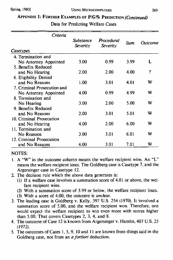
NOTES:1. A "W" in the outcome column means the welfare recipient wins. An "L"

means the welfare recipient loses. The Goldberg case is Casetype 7, and theArgersinger case in Casetype 12.

2. The decision rule which the above data generates is:(1) If a welfare case involves a summation score of 4.01 or above, the wel-

fare recipient wins.(2) With a summation score of 3.99 or below, the welfare recipient loses.(3) With a score of 4.00, the outcome is unclear.

3. The leading case is Goldberg v. Kelly, 397 U.S. 254 (1970). It involved asummation score of 5.00, and the welfare recipient won. Therefore, onewould expect the welfare recipient to win even more with scores higherthan 5.00. That covers Casetypes 2, 3, 4, and 8.

4. The outcome of Case 12 is known from Argersinger v. Hamlin, 407 U.S. 25(1972).

5. The outcomes of Cases 1, 5, 9, 10 and 11 are known from things said in theGoldberg case, not from an afortiori deduction.

Spring, 19851 USING MICROCOMPUTERS

AKRON LAW REVIEW

6. The above data comes from Nagel, Case Prediction by Staircase Tables andPercentaging, 25 JURIMETRICS 168 (1985).

Data for Predicting Equal Protection Cases

CriteriaScore On Score On Sum Outcome

Rights GroupsCasetypes

1. Consumers/Region 1 1 2 D2. Consumers/Economic Class 1 2 3 D3. Employment/Region 2 1 3 D4. Consumers/Sex 1 3 4 D5. Employment/Economic

Class 2 2 4 D6. Housing/Region 3 1 4 D7. Employment/Sex 2 3 5 D8. Housing/Economic Class 3 2 5 D9. Schools/Region 4 1 5 D

10. Housing/Sex 3 3 6 D11. Schools/Economic Class 4 2 6 D12. Consumers/Race 1 6 7 P13. Criminal Justice/Region 6 1 7 ?14. Schools/Sex 4 3 7 ?15. Criminal Justice/Economic

Class 6 2 8 P16. Employment/Race 2 6 8 P17. Voting/Region 7 1 8 P18. Criminal Justice/Sex 6 3 9 P19. Housing/Race 2 6 9 P20. Voting/Economic Class 7 2 9 P21. Schools/Race 4 6 10 P22. Voting/Sex 7 3 10 P23. Criminal Justice/Race 6 6 12 P24. Voting/Race 7 6 13 P

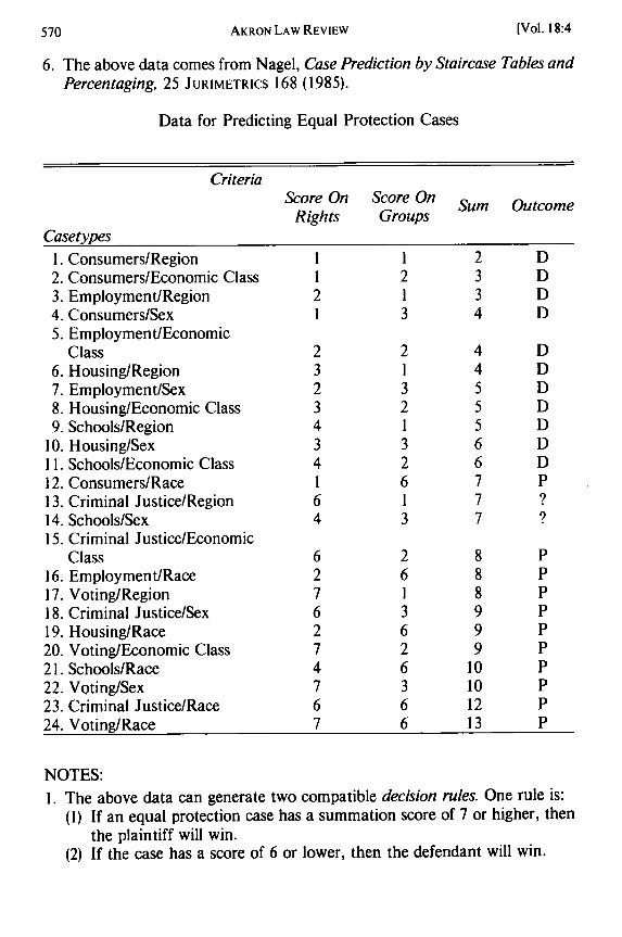
NOTES:1. The above data can generate two compatible decision rules. One rule is:

(1) If an equal protection case has a summation score of 7 or higher, thenthe plaintiff will win.

(2) If the case has a score of 6 or lower, then the defendant will win.

[Vol. 18:4

USING MICROCOMPUTERS

2. The alternative decision rule is:(1) If an equal protection case has a summation score greater than 7, then

the plaintiff will win.(2) If the case has a score of exactly 7, then the outcome is questionable.(3) If the case has a score of 6 or lower, then the defendant will win.

3. Each casetype is defined in terms of:(1) The rights that are allegedly being denied which can relate to voting,

criminal justice, schools, housing, employment, or consumer rights inthat order of importance.

(2) The group that is allegedly being given unequal treatment, which canrelate to race (which generally means being black), sex (which generallymeans being female), economic class (which generally means beingpoor), or region (which generally means being urban or inner city) inthat order of importance.

4. To determine the score of each casetype on the rights, the six rights are ar-ranged in rank order with the most important right receiving a score of 6.Slight adjustments are then made to recognize there is more distance be-tween the top two rights and the bottom four than there is between theother rights.

5. To determine the score of each casetype on the groups, the four groups arearranged in rank order with the most important group receiving a score of4. Slight adjustments are then made to recognize there is more distance be-tween the top group and the bottom three than there is between the othergroups.

6. The first decision rule implies that the court would decide in favor of theplaintiff if the state provided grossly unequal right to counsel from onecounty to another, or if women were denied admission to an all-male publicschool, although the court has not yet done so.

7. The second decision rule implies that being black scores slightly higher thana 6. That causes 12 to score slightly higher than 7, and thus to bedistinguishable from the questionable cases.

8. Landmark cases or Constitutional amendments that correspond to thecasetypes include Gomillio v. Lightfoot, 364 U.S. 339 (1960) (casetype 24);Powell v. Alabama, 287 U.S. 45 (1932) (casetype 23); U.S. CONST. amendXIX (casetype 22); Brown v. Bd. of Educ., 347 U.S. 483 (1954) (casetype21); Harper v. Virginia Bd. of Elections, 383 U.S. 663 (1966) (casetype 20);Shelley v. Kraemer, 334 U.S. 1 (1948) (casetype 19); Taylor v. Louisiana,419 U.S. 522 (1975) (casetype 18); Reynolds v. Sims, 377 U.S. 533 (1964)(casetype 17); Jones v. Alfred H. Mayer Co., 392 U.S. 409 (1968) (casetypes12 and 16); Gideon v. Wainwright, 372 U.S. 335 (1963) (casetype 15); andSan Antonio Ind. School Dist. v. Rodriguez, 411 U.S. 1 (1973), reh'gdenied, 411 U.S. 959 (1973).

9. The data for this table comes from Nagel, Case Prediction by StaircaseTables and Percentaging, 25 JURIMETRICS 168 (1985).

Spring, 19851

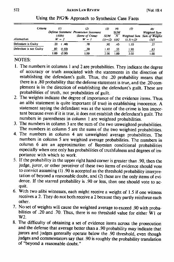
Using the PIG% Approach to Synthesize Case Facts

Criteria (I) (2) (3) (4) (5) (6)Defense Statement Prosecution Statement SUM Weighted Sum

(Alibi) (Scene of Crime) SUM N Weighted Sum Sum of WeightsAlternatives W = 2 W = I (l)+(2) (3Y2 (1.5)+(2) (5Y3Defendant is Guilty .20 ( .40) .70 .90 .45 1.10 .37Defendant is not Guilty .80 (1.60) .30 1.10 .55 1.90 .63

1.00 (2.00) 1.00 2.00 1.00 3.00 1.00

NOTES:1. The numbers in columns 1 and 2 are probabilities. They indicate the degree

of accuracy or truth associated with the statements in the direction ofestablishing the defendant's guilt. Thus, the .20 probability means thatthere is a .80 probability that the defense statement is true, and the .20 com-plement is in the direction of establishing the defendant's guilt. These areprobabilities of truth, not probabilities of guilt.

2. The weights indicate the degree of importance of the evidence items. Thusan alibi statement is quite important (if true) in establishing innocence. Astatement saying the defendant was at the scene of the crime is less impor-tant because even if it is true, it does not establish the defendant's guilt. Thenumbers in parentheses in column 1 are weighted probabilities.

3. The numbers in column 3 are the sum of the two unweighted probabilities.The numbers in column 5 are the sums of the two weighted probabilities.

4. The numbers in column 4 are unweighted average probabilities. Thenumbers in column 5 are weighted average probabilities. The numbers incolumn 6 are an approximation of Bayesian conditional probabilitiesespecially when one only has probabilities of truthfulness and degrees of im-portance with which to work.

5. If the probability in the upper right hand corner is greater than .90, then thejudge, juror, or other perceiver of these two items of evidence should voteto convict assuming (1) .90 is accepted as the threshold probability interpre-tation of beyond a reasonable doubt, and (2) these are the only items of evi-dence. If the starred probability is .90 or less, then one should vote to ac-quit.

6. With two alibi witnesses, each might receive a weight of 1.5 if one witnessreceives a 2. They do not both receive a 2 because they partly reinforce eachother.

7. No set of weights will cause the weighted average to exceed .90 with proba-bilities of .20 and .70. Thus, there is no threshold value for either W1 orW2.

8. The difficulty of obtaining a set of evidence items across the prosecutionand the defense that average better than a .90 probability may indicate thatjurors and judges generally operate below the .90 threshold, even thoughjudges and commentators say that .90 is roughly the probability translationof "beyond a reasonable doubt."

AKRON LAW REVIEW [Vol. 18:4

USING MICROCOMPUTERS

APPENDIX 2. THE COMPUTER OUTPUT FOR GOING FROM CASES, CRITERIA, ANDSCORES TO A PREDICTIVE CONCLUSION

The Nine Redistricting Cases and How They Were Decided

PreviousAlternative OutcomeI. Colegrove D Wins2. Grills A3. Maryland D4. Scholle D5. WMCA D6. Asbury A7. Dyer A8. Baker A9. Magraw A

NOTE:I. These are nine key cases on the subject of legislative redistricting decided between Colegrove v. Green,

328 U.S. 549 (1946) and Baker v. Carr, 369 U.S. 186 (1962).

The Four Predictive Criteria and How They Are Measured and Weighted

Criterion Meas. Unit Weight1. = Required Yes/2 No/I 1.002. State Legis. 1.003. = Violated 1.004. Fed. Court 1.00

NOTES:1. The first criterion is whether or not the relevant constitution required equal population per legislative

district.2. The second criterion is whether the legislature in question was a state legislature or the federal Congress.3. The third criterion is whether the degree of equality violation is great enough that less than 35% of the

state's population could choose more than 50% of the legislative body or congressional delegation.4. The fourth criterion is whether the court deciding the case was a federal or state court.5. All the criteria are worded so that a yes answer is favorable to a victory for the side attacking the prevail-

ing redistricting.

The Scores of the Cases on the Criteria

Alternative/Criteria Scoring= Requi State Le = Viola Fed. Cour

Colegrove 1.00 1.00 1.00 2.00Grills 2.00 2.00 1.00 1.00Maryland 1.00 2.00 2.00 1.00Scholle 1.00 2.00 2.00 1.00WMCA 1.00 2.00 1.00 2.00Asbury 2.00 2.00 2.00 1.00Dyer 2.00 1.00 2.00 2.00Baker 2.00 2.00 2.00 2.00Magraw 2.00 2.00 2.00 2.00

Spring, 1985]

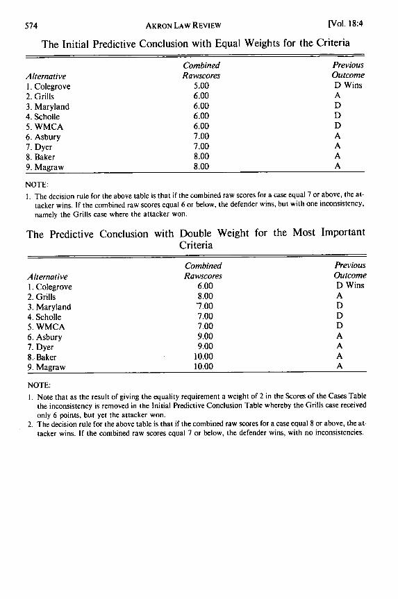
The Initial Predictive Conclusion with Equal Weights for the Criteria

Combined PreviousAlternative Rawscores Outcome

1. Colegrove 5.00 D Wins2. Grills 6.00 A3. Maryland 6.00 D4. Scholle 6.00 D5. WMCA 6.00 D6. Asbury 7.00 A7. Dyer 7.00 A8. Baker 8.00 A9. Magraw 8.00 A

NOTE:1. The decision rule for the above table is that if the combined raw scores for a case equal 7 or above, the at-

tacker wins. If the combined raw scores equal 6 or below, the defender wins, but with one inconsistency,namely the Grills case where the attacker won.

The Predictive Conclusion with Double Weight for the Most ImportantCriteria

Combined PreviousAlternative Rawscores OutcomeI. Colegrove 6.00 D Wins2. Grills 8.00 A3. Maryland 7.00 D4. Scholle 7.00 D5. WMCA 7.00 D

6. Asbury 9.00 A7. Dyer 9.00 A8. Baker 10.00 A9. Magraw 10.00 A

NOTE:

1. Note that as the result of giving the equality requirement a weight of 2 in the Scores of the Cases Tablethe inconsistency is removed in the Initial Predictive Conclusion Table whereby the Grills case receivedonly 6 points, but yet the attacker won.

2. The decision rule for the above table is that if the combined raw scores for a case equal 8 or above, the at-tacker wins. If the combined raw scores equal 7 or below, the defender wins, with no inconsistencies.

[Vol. 18:4AKRON LAW REVIEW