using passive acoustics to model blue whale habitat off...

Deep-Sea Research II 58 (2011) 1719–1728

Contents lists available at ScienceDirect

Deep-Sea Research II

0967-06

doi:10.1

n Corr

E-m

journal homepage: www.elsevier.com/locate/dsr2

Using passive acoustics to model blue whale habitat off the WesternAntarctic Peninsula

Ana Sirovic n, John A. Hildebrand

Scripps Institution of Oceanography, UCSD, 9500 Gilman Drive 0205, La Jolla, CA 92093-0205, USA

a r t i c l e i n f o

Article history:

Received 14 October 2008

Received in revised form

27 January 2010

Accepted 2 August 2010Available online 16 December 2010

Keywords:

Blue whales

Passive acoustics

Antarctica

Habitat modeling

SO GLOBEC

45/$ - see front matter & 2010 Elsevier Ltd. A

016/j.dsr2.2010.08.019

esponding author. Tel.: +1 8585348210.

ail address: [email protected] (A. Sirovic).

a b s t r a c t

Habitat preferences of calling blue whales were investigated using data from two multidisciplinary

oceanographic cruises conducted off the Western Antarctic Peninsula (WAP) during the austral falls of

2001 and 2002. Data were collected on depth, temperature, salinity, chlorophyll a (Chl-a) concentration,

krill biomass, zooplankton abundance, and blue whale call presence. In 2001, the study area was sea ice

free, high Chl-a concentrations occurred over a small area, krill biomass and zooplankton abundance were

high, and few blue whale calls were detected. In 2002 the sea ice covered the southern part of the survey

area, Chl-a was high over a large area, krill and zooplankton were low, and there were more blue whale

calls. Logistic regression analysis revealed blue whale calls were positively correlated with depth and SST,

and negatively correlated with the mean zooplankton abundance from 101 to 300 m and the mean krill

biomass in the top 100 m. The negative correlation between blue whale calls and zooplankton could occur

if feeding animals do not produce calls. Our survey area did not cover the full range of blue whale habitat

off the WAP, as blue whales probably follow the melting and freezing ice edge through this region. Passive

acoustics can provide insight to mesoscale habitat use by blue whales in the Southern Ocean where visual

sightings are rare, but the ability to localize on the calling animals would greatly improve the ability to

model at a finer scale.

& 2010 Elsevier Ltd. All rights reserved.

1. Introduction

The earliest scientific understanding of baleen whale habitatassociations came from the Discovery investigations of the 1930s,the goal of which was a systematic exploration of the SouthernOcean resources, particularly ones linked to the whaling industry.Well-known whaling grounds were associated with prominentatmospheric and physical features (Kellogg, 1929; Beklemishev,1960), as well as high abundance of krill (Marr, 1962) that are theprimary food source for baleen whales in the Southern Ocean(Mackintosh and Wheeler, 1929; Mackintosh, 1965; Kawamura,1994a).

Southern Ocean productivity is affected by circulation patterns andsea ice dynamics (Nicol et al., 2000; Constable et al., 2003). Off theAntarctic Peninsula, the Antarctic Circumpolar Current (ACC) bringsintrusions of oceanic, relatively warm (1.5–2 1C), and salty (34.6–34.7)water, Upper Circumpolar Deep Water (UCDW), on the shelf (Klincket al., 2004). The larger Marguerite Bay shelf area (Fig. 1) gets entirelycovered by the sea ice in the winter (Stammerjohn and Smith, 1996).These shelf regions generally have higher rates of primary productivitythan open waters off the shelf (Holm-Hansen et al., 1997; Constable

ll rights reserved.

et al., 2003) and feature relatively high krill biomass (Marr, 1962;Lascara et al., 1999; Atkinson et al., 2004) important for feeding whales(Kawamura, 1994b).

Blue whales (Balaenoptera musculus) are generally found in theSouthern Ocean in the spring and the summer and are thought tomigrate to lower latitudes in the fall (Mackintosh, 1965; Kasamatsuet al., 1988, 1996; Branch et al., 2007). While in the Antarctic, they mayundertake extensive circumpolar movement (Brown, 1954, 1962;Branch et al., 2007). Based on acoustic recordings, blue whales canbe heard in the Antarctic year-round (Sirovic et al., 2004, 2009).

Blue whales are relatively rarely sighted in the Southern Ocean(Branch and Butterworth, 2001; Thiele et al., 2004), but they can bereliably detected from their calls (Sirovic et al., 2004, 2006). Bluewhales in the Southern Ocean produce several call types (Ljungbladet al., 1998; Rankin et al., 2005). One type, the ‘‘28 Hz tonal’’, is up to18 s long, consists of a tone generally followed by down sweptsegments, and is often repeated at regular intervals (Sirovic et al.,2004; Rankin et al., 2005). Similar low frequency, repetitive calls(termed songs) produced by blue whales off California are attrib-uted to males and are presumed to function as mating displays(McDonald et al., 2001; Oleson et al., 2007a). Blue whales alsoproduce variable, frequency modulated ‘‘D calls’’ that last up to 4 sand sweep downward in frequency from approximately 100 to 40 Hz(Thompson et al., 1996; Rankin et al., 2005; Sirovic et al., 2006).D calls off California and in the Southern Ocean have been associated

www.elsevier.com/locate/dsr2

dx.doi.org/10.1016/j.dsr2.2010.08.019

mailto:[email protected]

mailto:[email protected]

dx.doi.org/10.1016/j.dsr2.2010.08.019

Fig. 1. Survey area of the US Southern Ocean GLOBEC cruises, with color from red to

violet indicating increasing depths, land is white. Approximate depths: orange

200 m, dark blue 3000 m. Stars represent locations of CTD survey stations (for

interpretation of the references to color in this figure legend, the reader is referred to

the web version of this article).

A. Sirovic, J.A. Hildebrand / Deep-Sea Research II 58 (2011) 1719–17281720

with feeding blue whales and are produced by both sexes (Rankinet al., 2005; Oleson et al., 2007a).

Recent integrative ecology work in the Southern Ocean has focusedon humpback (Megaptera novaeangliae) and Antarctic minke whales(Balaenoptera bonaerensis), which are more abundant there than bluewhales (Moore et al., 1999; Branch and Butterworth, 2001; Muraseet al., 2002; Thiele et al., 2004; Friedlaender et al., 2006, 2009). Thecontinental slope that coincides with the ice edge is an importantfeeding ground for minke whales, while humpback whales areassociated with the areas of high krill and chlorophyll a density(Nicol et al., 2000; Murase et al., 2002). In the WAP region, bothhumpback and minke whale distributions are influenced by zooplank-ton presence as measured by volume backscatter, distance to the iceedge, and bathymetry (Friedlaender et al., 2006). Spatially explicitanalytical techniques quantify relationships between cetacean speciesand their environment and generate predictive habitat models ofcetacean use (see Redfern et al. (2006) for a review of this topic).

The Southern Ocean Global Ocean Ecosystems Dynamics(SO GLOBEC) program was designed to test hypotheses about theinteractions between the Antarctic krill (Euphausia superba) and theirenvironment and predators, and provide a benchmark for futuremultidisciplinary research in the Antarctic (Hofmann et al., 2002). Thefield program consisted of multiple, multidisciplinary oceanographiccruises along the WAP. The goal of this study was to investigatethe possibility for using passive acoustics to study the mesoscale(10–100 km) habitat of blue whales. This scale corresponds with thetypical range of several tens of km expected for acoustic survey ofbaleen whales using sonobuoys (McDonald, 2004). We describe therelationship between the distributions of calling blue whales and thephysical and biological variables in the US Southern Ocean GLOBECstudy area on the WAP shelf in the austral falls of 2001 and 2002. Inparticular, the relationships with bathymetry, sea ice and sea surfacetemperature (SST), UCDW intrusions, surface chlorophyll a concen-trations, krill biomass and abundance of other zooplankton (e.g.copepods and siphonophores) and fish were investigated. Advantagesand limitations of using passive acoustics for whale habitat modelingare discussed.

2. Methods

Data were collected during two SO GLOBEC survey cruisesaboard the RVIB Nathaniel B. Palmer in the Western AntarcticPeninsula region near Marguerite Bay: from 23 April to 6 June 2001and from 9 April to 21 May 2002. The surveys were designed toprovide a broad-scale, synoptic look at an area approximately240 km�480 km (Fig. 1) by collecting data on the hydrography,nutrients, primary production, zooplankton, and top-predatordistribution characteristics. In these analyses, only the data fromthe southward pass through the survey grid were used to ensurecontemporaneous oceanographic and acoustic data during eachyear. In this paper, when referring to the survey year, it is implicitthat the periods discussed are the survey months of April and May,not the entire year.

2.1. Environmental data collection

Hydrographic data collected during the two surveys coveredmuch of the same area on the WAP shelf, north and south ofMarguerite Bay, as well as within the Bay. The survey started at thenorth end of the region and moved southward in both years.Thirteen cross-shelf transects were conducted perpendicular to thecoastline and the shelf break. Stations were mostly spaced at 40 kmintervals, with some stations at 10 km intervals to provide finerresolution of rapidly changing areas, such as the shelf break region(Klinck et al., 2004). The southbound survey consisted of 81hydrographic stations in 2001, and 92 stations in 2002. Tempera-ture and salinity measurements were made using a SeaBird911+Niskin/Rosette conductivity–temperature–density (CTD)sensor system. The Rosette system consisted of 24 10-liter Niskinbottles and water samples were taken at standardized depths.Chlorophyll a concentrations were measured from the watersamples using a Turner Designs Digital 10-AU-05 Fluorometer.In this study, sea surface temperature (SST) and surface chlorophylla (Chl-a) concentration were reported. Also, the temperaturemaximum below 200 m depth (Tmax200), and the salinity at 50 m(Sal50) were determined. Tmax20041.8 1C is representative of theACC waters, and the waters with Tmax200 between 1.5 and 1.8 1C areindicative of the UCDW (Klinck et al., 2004). Bathymetry data werecollected using a SeaBeam multibeam system mounted on the hullof the ship (Bolmer et al., 2004).

Acoustic backscatter and target strength data were collectedusing BIOMAPER-II, which was equipped with five pairs of trans-ducers with center frequencies at 43, 120, 200, 420 kHz, and 1 MHz(Lawson et al., 2004). BIOMAPER-II was ‘‘tow-yoed’’ up and downthrough the water column between 20 and 400 m depths, while theship was steaming between the hydrographic stations at speeds of4–6 kts. Acoustic methods were developed from measurements ofvolume backscatter and target strength at 43 and 120 kHz, yieldingestimates of krill biomass (Lawson, 2006; Lawson et al., 2007a).Krill were separated from the rest of the zooplankton because theyare the primary prey species for blue whales in the Southern Ocean(Kawamura, 1980; Kawamura, 1994a). The remainder of thevolume backscatter signal was used as a proxy for other zooplank-ton species with different target strengths, such as copepods andsiphonophores, and also included fish (Ashjian et al., 2004; Lawsonet al., 2004). Details on acoustic methods for estimation of krillbiomass and the limitations and uncertainties in the available dataare detailed in Lawson et al. (2004, 2007a) and Lawson (2006).Mean volume backscatter (dB) and krill biomass (g m�2) wereintegrated over 0–100 and 101–300 m and averaged over the20 km along-track intervals centered at the passive acousticreceiver (sonobuoy) deployment locations for which BIOMAPER-IIdata were available. This yielded 36 and 41 points with concurrent

A. Sirovic, J.A. Hildebrand / Deep-Sea Research II 58 (2011) 1719–1728 1721

active and passive acoustic data in 2001 and 2002 survey years,respectively, which were used for model development. Hydro-graphic data from CTD stations were used for estimation oftemperature, salinity, and chlorophyll a concentration at sonobuoydeployment locations as well, using the IDW interpolation methoddiscussed in Section 2.3.

2.2. Passive acoustic data collection and analysis

Blue whale calls were analyzed from sonobuoy recordings madeduring two survey cruises. Sonobuoys are expendable, radio-linkedunderwater listening devices that were deployed when whaleswere visually detected, before CTD stations, and sporadicallythroughout the cruises, to provide coverage of the entire surveyedarea. Both omnidirectional (AN/SSQ-57B) and directional sono-buoys (DIFAR, AN/SSQ-53D) were used. Omnidirectional sono-buoys have a broader frequency response than the directionalsonobuoys (10–20,000 and 10–2400 Hz, respectively), but thelatter type provide data on the sound source direction. A total of59 sonobuoys were deployed on the southbound pass of the 2001cruise: 2 omnidirectional and 57 DIFAR. During the southboundportion of the 2002 cruise, a total of 47 sonobuoys were deployed:44 omnidirectional and 3 DIFAR. A total of 4 omnidirectional and3 DIFAR sonobuoys failed upon deployment during these cruises,giving a failure rate of 9% and 5%, respectively.

Custom electronics and software were used to record and analyzesonobuoy data during and after the cruises. Two antennae wereavailable for the reception of the sonobuoy radio signal aboard theRVIB Nathaniel B. Palmer: a 162–173.5 MHz eight-element directionalYagi and a 138–174 MHz two dipole omnidirectional SRL-210-A2Sinclair antenna. The maximum range for the radio transmissionduring these cruises was 16 nmi for the Yagi, and 10 nmi for theSinclair, but the range was dependent on the weather conditions. Weused software controlled ICOM IC-PCR1000 scanner radio receiver,modified to provide improved low frequency response, for the recep-tion of the sonobuoy signal. Data were recorded continuously to digitalaudiotapes at 48 kHz sample rate using Sony PCM-300 and PCM-M1digital audio recorders during 2001 and 2002 cruises, respectively.Upon each deployment the following information was recorded: time,latitude, longitude, and bottom depth at deployment, sonobuoy typeand channel, reason for deployment (whale sighting, CTD station, etc.).Also, ship speed and course, and general weather and sea ice conditionswere noted. After deployment, the sonobuoys transmitted their radiosignal to the underway ship for a maximum of 8 h before scuttling andsinking. Duration of recording per sonobuoy varied depending on otheractivities occurring on the ship and ranged between 1 and 8 h.

After the cruise, data were digitized and converted into 35 minwav files by playing the audiotapes on a Sony PCM-M1 and re-digitizing the analog signal using the real-time signal recordingfeature in software program Ishmael (Mellinger, 2001). Since the

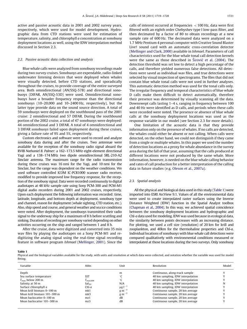
Table 1Physical and the biological variables available for the study, with units and resolution at

fitting.

Variable Abbr. Unit

Depth m

Sea surface temperature SST 1C

Tmax below 200 m Tmax200 1C

Salinity at 50 m Sal50 N/A

Surface chlorophyll a Chl-a mg l�1

Mean krill biomass 0–100 m mk1 g m�2

Mean krill biomass 101–300 m mk3 g m�2

Mean backscatter 0–100 m mz1 dB

Mean backscatter 101–300 m mz3 dB

calls of interest occurred at frequencies o100 Hz, data were firstfiltered with an eighth order Chebyshev type I low-pass filter, andthen decimated by a factor of 80 to obtain recordings at a newsample rate of 600 Hz. The decimated data were analyzed on a1.7 MHz Pentium 4 personal computer with Creative Sound BlasterLive! sound card with an automatic cross-correlation detector(Mellinger and Clark, 2000) available in Ishmael. Parameters of callcharacteristics used for the blue whale tonal call detection kernelswere the same as those described in Sirovic et al. (2004). Thedetection threshold was set low to detect a high percentage of thecalls, and therefore yielded numerous false detections. All detec-tions were saved as individual wav files, and true detections wereselected by visual inspection of spectrograms. The files that did notcontain blue whale tonal calls were not used in further analyses.This automatic detection method was used for the tonal calls only.The irregular frequency and temporal characteristics of blue whaleD calls make them difficult to detect automatically, thereforetheir presence was determined by visually scanning all the data.Downswept calls lasting 1–4 s, ranging in frequency between 100and 40 Hz were identified as D calls, and periods when these callswere recorded were noted. The presence or absence of blue whalecalls at the sonobuoy deployment locations was used as theresponse variable in our model (see Section 2.3 for more details).

One limitation of the acoustic data is that they provideinformation only on the presence of whales. If no calls are detected,the whales could either be absent or not calling. When calls weredetected, on the other hand, we could not distinguish if they camefrom a single or multiple whales. In this paper we used the numberof detection locations as a proxy for whale abundance in the surveyarea during the fall of that year, assuming that the calls produced atdifferent locations were not produced by the same whale. Moreinformation, however, is needed on the blue whale calling behaviorand rates of call production for a better interpretation of the callingdata in future studies (e.g. Oleson et al., 2007a).

2.3. Spatial analysis

All the physical and biological data used in this study (Table 1) wereimported into ESRI ArcView 9.1. Values of all the environmental datawere used to create interpolated raster surfaces using the InverseDistance Weighted (IDW) function in the Spatial Analyst toolbox(Chapman et al., 2004). In this way, we achieved spatial coincidencebetween the sonobuoy deployment locations and hydrographic andChl-a data used for modeling. IDW was used because in ecological data,the similarity between points decreases with an increasing distance.For plotting, we used a cell size (resolution) of 20 km for krill andzooplankton, and 40km for the thermohaline properties and Chl-a.Individual locations of sonobuoys with blue whale call detections werecompared qualitatively with environmental conditions measured orinterpolated at those locations during the two surveys. Only sonobuoy

which data were collected, and notation whether the variable was used for model

Resolution Model

Continuous, along-track sample Y

40 km sampling, IDW interpolation Y


40 km sampling, IDW interpolation N


Continuous sample, 20 km average Y





deployment locations that had concurrent active acoustic data andhydrographic data were used for modeling.

We used logistic regression to explore the quantitative nature of therelationship between whale call presence and the environmentalvariables. Due to the small number of blue whale detections in 2001and small number of locations with D calls in both years, data for thetwo years and different call types were pooled. Additionally, pooling ofdata across years allows for a development of a more robust model thatis not limited to conditions from one year. A null model was built basedonly on the presence of calling blue whales at each sonobuoy, with anassumed binomial error structure. Correlations between environmen-tal variables were calculated to check for colinearity and only variableswith correlation o0.7 were used in model fitting (Weisberg, 2005).A forward–backward stepwise selection process was used to find themodel with the best fit to the data from the available variables. The bestmodel fit was determined using Akaike’s Information Criterion (AIC) ateach step. The added contribution of each variable to the model fit wasevaluated from the change in the deviance by the addition of thatvariable. Since AIC has a tendency to over-fit the data, all the variableswere sequentially tested for significance (a¼0.05) using a w2-test forreduction of overall deviance (McCullagh and Nelder, 1989). Wecalculated the squared multiple correlation coefficient, R2, to estimatethe proportion of the variation in the presence or calling blue whalesexplained by the final model. The final model was checked forautocorrelation in the residuals and the regression coefficients werestandardized to the same units for easier inter-comparison (Selvin,1998). All the analyses were done using S-PLUS 6 for Windows.

3. Results

3.1. Qualitative comparison

The overall hydrographic and biological conditions were verydifferent between the two survey years. In 2001, the sea ice formedrelatively late (Perovich et al., 2004). Even though the 2001 cruisestarted two weeks later in the season than in 2002, no sea ice hadformed during the former, but by the time of the latter cruise, the sea icehad already covered the southern portion of the survey area. In the fallof 2002, the krill biomass was 0 mg m�2 across a large part of thesurvey area that had at least 6 mg m�2 in 2001 (Lawson et al., 2004,2007b). High zooplankton abundance occurred over a larger area in2001. The maximum observed values of Chl-a were similar betweenyears, but in 2002, high levels of Chl-a extended further south andcloser inshore. More blue whale calls were detected in 2002, but no

Fig. 2. Areas with high calling blue whale presence during the two survey years are shown

during that survey. Black areas represent land.

blue whales were sighted by experienced marine mammal visualobservers during either cruise (Thiele et al., 2004). During both yearsthe ACC was flowing just off the shelf break and there was evidence ofthe UCDW intrusions onto the shelf.

There were distinct differences in the distribution of calling bluewhales between the years. In 2001, blue whale calls were detected onjust three sonobuoys (Fig. 2). On one sonobuoy, deployed off the shelfbreak in the middle of the survey area, the calls were ‘‘28 Hz tonals’’ (forsimplicity referred to as ‘‘tonals’’ through the rest of the paper). D callswere detected on two different sonobuoys, deployed in the vicinity ofAlexander Island. In 2002, blue whale tonal calls were detected on 21sonobuoys, mostly in the northern and middle shelf areas. Also, D callswere detected on four of those sonobuoys. The sonobuoys on whichcalls were detected were deployed along Marguerite Trough, thetrough west of Alexander Island, and off the shelf break (Fig. 2).

In 2001, the survey area had SST 4�1.7 1C and was largely free ofthe sea ice (Fig. 3; Thiele et al., 2004; Friedlaender et al., 2006). SST waslower than �1.7 1C and the sea ice covered the southern part ofMarguerite Bay and much of the southwestern portion of the surveygrid in the fall of 2002 (Thiele et al., 2004). All the whale call detectionsoccurred in ice-free waters, but there were more detections in the yearwhen the sea ice was already forming. Fig. 4 shows the ACC(Tmax20041.8 1C) flowing just off the shelf break during both surveys,with a somewhat stronger signal in 2002. During both surveys, theUCDW intrusions onto the shelf occurred along Marguerite Trough,starting at the shelf break in the northwest end of the survey area, andextending into the Bay along the western side of Adelaide Island. Mostblue whale calls were associated with the regions of the ACC and theUCDW intrusions (Fig. 4).

The maximum surface Chl-a values were similar between thetwo years (2.01 and 2.16 mg l�1 in 2001 and 2002, respectively), butduring 2002, high Chl-a concentrations extended over a larger area(Fig. 5). In 2001, the blue whale call detections occurred outside theareas of high Chl-a. In 2002, blue whale call detections occurredboth in areas of high and low Chl-a concentrations.

Krill had higher biomass and zooplankton had higher abun-dance in 2001 than 2002 (Figs. 6–9). Generally, in both years,the highest concentrations occurred on the northwest side ofAlexander Island, along the west and north shores of Adelaide Island,and in south Marguerite Bay. Both the mean krill biomass and themean zooplankton abundance were higher in the 100–300 m depthrange than in the top 100 m. The highest krill biomass occurred offthe western Alexander and the northern Adelaide Islands in bothyears (Figs. 6 and 7). In 2002, the zooplankton abundance in the top100m was high in the southwestern parts of the survey area, with

with darker shading based on IDW. Pluses are locations of all sonobuoy deployments

Fig. 3. Sea surface temperature (sea ice cover proxy) during the two survey years, smoothed with IDW. Stars represent locations of CTD survey stations. Blue squares are

sonobuoy deployment locations on which blue whale tonals were detected and blue triangles are blue whale D call locations. Black areas represent land.

Fig. 4. Temperature maximum below 200 m (UCDW proxy) during the two survey years, smoothed with IDW. Symbols are the same as in Fig. 3.

Fig. 5. Surface chlorophyll a concentrations during the two survey years, smoothed with IDW. Symbols are the same as in Fig. 3.


Fig. 6. Mean krill biomass in the top 100 m during the two survey years, smoothed with IDW. Pluses represent center locations of the 20 km along-track intervals over which

the mean krill biomass was calculated. Blue squares are sonobuoy deployment locations where blue whale tonals were detected and blue triangles are blue whale D call

locations. Black areas represent land.

Fig. 7. Mean krill biomass at depth (101–300 m) during the two survey years, smoothed with IDW. Symbols are same as in Fig. 6.


the highest values at the southeastern end of Marguerite Bay(Fig. 8). In 2001, the zooplankton abundance at depth (101–300 m)was high in most of the survey region, peaking at the southern end(Fig. 9). In both years, small krill aggregations dominated numeri-cally, but the small numbers of very large aggregations contributedthe majority of the biomass (Lawson, 2006).

In 2001, blue whale D calls were detected twice in the area withthe highest krill biomass and zooplankton abundances, but the nextyear, D calls were detected in the areas of low krill biomass andzooplankton abundances. In 2002, the northwest shelf, where mostblue whale tonal calls were detected, had 0 g m�2 krill biomass. Allother regions where blue whale tonals and D calls were detectedthat year had low krill biomass, as well, both in the surface 100 mand in the 100–300 m depth range (Figs. 6 and 7).

3.2. Modeling results

Eight of the available nine environmental variables were used forthe model fitting (Table 1). Tmax200 and Sal50 had a correlation of 0.740,

indicating they are both related to the UCDW intrusions, so only Tmax200

was used in the model selection process. The variables that were foundto be significantly explanatory of the calling blue whale presence were:depth, the mean krill biomass in the 0–100 m range, the meanzooplankton abundance in the 101–300 m range, and the sea surfacetemperature (w2

¼49.179, df¼4, po0.0001; Table 2). Depth and thesea surface temperature were positively correlated with the presence ofthe calling blue whales, and krill and zooplankton were negativelycorrelated (Fig. 10; Table 2). This model explained almost 59% of theblue whale call presence data (R2

¼0.587).

4. Discussion

These results come from the first fall surveys in larger Marguer-ite Bay area that combined blue whale presence data with theenvironmental data since the Discovery expedition. They offered anuncommon opportunity to investigate distribution patterns bycalling blue whales in the Southern Ocean. While some mesoscale

Fig. 8. Mean zooplankton abundance in the top 100 m during the two survey years, smoothed with IDW. Symbols are the same as in Fig. 6.


use patterns can be gleaned from passive acoustic data for this typeof modeling, the interpretation of the data was limited by theconstraints imposed by the differences in scales at which differentdata were collected, which are fully addressed in Section 4.2.

These fall surveys showed a high degree of interannual varia-bility in this region of the Southern Ocean. One notable difference inthe conditions between the two years was the timing of the sea iceformation (Perovich et al., 2004). The sea ice cycle is an importantfeature that affects physical and biological processes (Nicol et al.,2000; Nicol, 2006) and the sea ice cover differences between thesurveys were broadly paralleled by the differences in the distribu-tion and abundance of Chl-a, krill, zooplankton and calling whales.Consistent between the years, however, high krill and zooplanktonabundances coincided with the areas of steep bathymetry, such asMarguerite Trough (Ashjian et al., 2004; Lawson et al., 2004).

The negative relationship we found between the calling bluewhales and the krill and zooplankton could indicate that the callingblue whales are not feeding. In addition to this negative relation-ship between the calling blue whales and the zooplankton, therewas also an apparent negative relationship between the zooplank-ton and Chl-a (Lawson, 2006). This may indicate a degree of top-down control in the area, with zooplankton depleting the Chl-a andblue whales depleting the zooplankton (Beklemishev, 1960;Carpenter et al., 1985). The linkage between Chl-a and the callingblue whales, however, was not significant.

Humpback and Antarctic minke whale habitat preferences wereanalyzed previously from the sighting data collected during thesame two surveys (Friedlaender et al., 2006). As for the blue whales,the distribution of humpback and minke whales was related to theice edge and bathymetry, but humpback and minke whales had apositive relationship with zooplankton. These analyses, however,were based on sighting data, not acoustic detections. Differentbaleen whale survey methods (visual versus acoustic) may sampleanimals in different behavioral states (Oleson et al., 2007b, 2007c),which could account for the differences in their zooplanktonlinkages.

4.1. Blue whale distribution

Correlations between the calling blue whale distribution and thebathymetry and the SST were also found in the North Pacific (Croll et al.,1998; Fiedler et al., 1998). The difference was that in temperate andtropical regions, the SST was negatively correlated with the blue whale

distribution. All the whale detections in this study occurred in thewarmer, ice-free waters. This difference in the direction of thecorrelation is likely due to the fact that in the polar region in the fall,a low surface temperature is not an expression of the upwelled,nutrient rich waters, but rather indicates sea ice formation. So eventhough the SST appears to be an important predictor of blue whalehabitat in a variety of environments, the underlying ecology differs.

A number of studies found that rorquals in different geographicregions are associated with their prey at various scales, ranging from afew km to thousands of km (Croll et al., 1998; Tynan, 1998; Nicol et al.,2000; Reid et al., 2000; Friedlaender et al., 2006). Positive correlations atfine scales are harder to demonstrate (Reid et al., 2000; Baumgartneret al., 2003), but the scale used in this study (10 s of km) should be largeenough to test the general relationships between the whales and thekrill. The negative correlation between the calling blue whales and krillbiomass and zooplankton abundance could be the result of severalfactors. In 2002, the krill biomass in much of the northern part of thesurvey area, where most blue whale calls were detected, was 0 g m�2.Although it is possible that existing krill patches were missed by thevery narrow BIOMAPER-II tracks, the consistent absence of krill overseveral track lines strengthens the idea there were no krill in this region.

Blue whales come to the Southern Ocean primarily to feed(Kawamura, 1994b), but they most likely do not spend all their timeforaging. Therefore, it is necessary to consider other behavioral contextsof whale presence in the WAP region. Evidence from California suggeststhat blue whales producing tonal, song-like calls may not be feeding,but are moving through the area (McDonald et al., 1995; Oleson et al.,2007a). Thus, we should not always expect to find calling blue whalesin areas with high krill biomass. Blue whales making D calls are morelikely to be feeding (Oleson et al., 2007a, 2007c). Rankin et al. (2005)recorded both tonal and D calls in the vicinity of apparently feedinganimals during the austral summer. During our surveys, two out of sixtimes blue whale D calls were detected, they were associated with highkrill biomass and zooplankton abundance. It has been found previouslythat blue whales are tightly linked to krill in the Antarctic during thespring and the summer (Hardy and Gunther, 1935), but it is possiblethat by the fall, the whales are well fed and, as the krill move into thecoastal regions (Lascara et al., 1999; Lawson, 2006), the whales startengaging more in other behaviors, such as tonal calling, which may alsobe linked to swimming or migration out of the area or pairing inpreparation for mating (McDonald et al., 1995; Oleson et al., 2007a).This shift in behavior could explain some of the seasonal differencesnoted in the long-term abundance of blue whale calls off the WAP

Fig. 9. Mean zooplankton abundance at depth (101–300 m) during the two survey years, smoothed with IDW. Symbols are the same as in Fig. 6.

Table 2Results of the stepwise linear regression modeling, showing all the significant

variables: mz3 is the mean backscatter in the 101–300 m depth range, mk1 is the

mean krill biomass from 0 to 100 m depth, and SST is sea surface temperature.

Model Coefficient df Deviance p-Value

Normal 76 83.743

+Depth 0.582 75 71.536 0.0005

+mz3 �2.481 74 58.051 0.0002

+mk1 �32.560 73 45.248 0.0003

+SST 1.458 72 34.564 0.0011


(Sirovic et al., 2004) and the lack of blue whale calls in December, whenwhales may be mostly feeding.

If we assume feeding and tonal calling are mutually exclusive, lowwhale call detections in 2001 could indicate the whales were stillfeeding at the time of the survey cruise. Alternatively, they could havebeen closer to the ice edge which they might be using as a reliablelocation of aggregated prey (Brierley et al., 2002; Nicol, 2006). Oursurvey certainly covered smaller area than the total area used by theforaging blue whales in the WAP region. The temporally bimodaldistribution of blue whale calls recorded on bottom-moored instru-ments in the larger WAP area (Sirovic et al., 2004) indicates that thewhales could be moving through our survey area with the retreatingand advancing ice edge. If the whales are simply swimming when theyproduce tonal calls, we would not expect to find any association withprey aggregations. The presence of a negative correlation, however,may imply that the production of blue whale tonal calls in the WAP inthe fall indicates the end of foraging.

4.2. Data limitations

There were several problems associated with the interpretationof acoustic volume backscatter data collected during these surveys.The 43 kHz transducer did not function properly in 2001 and,therefore, krill biomass data were not as reliable as in 2002(Lawson, 2006). Also, while it is clear that E. superba is the primaryprey species of blue whales in the Southern Ocean (Kawamura,1994a), it is unclear which krill species were observed with activeacoustics. Size estimates from the acoustic data, as well as net towsand Video Plankton Recorder data, indicate that deep, dense, costal

patches, that dominate biomass estimates, are likely E. superba

(Ashjian et al., 2004; G. Lawson, pers. comm.), but some aggrega-tions off Alexander Island could have been E. crystallorophias

(Ashjian et al., 2004). Information on zooplankton species compo-sition would be useful for a more accurate interpretation of thenegative relationships between the calling whales and krill andother zooplankton.

There was a mismatch between the scales over which BIOMAPER-IIand hydrographic data were collected, and the ranges over which bluewhales could be detected. Temperature, salinity and Chl-a data werecollected mostly at 40 km intervals. BIOMAPER-II data were collectedcontinuously along transects, but they were subsequently averagedover 20 km, centered at the sonobuoy deployment locations. Bluewhale calls in the Southern Ocean propagate over long distances (up to100 km, Sirovic et al., 2007) and the sonobuoy monitoring range in thisstudy extended over tens of km (McDonald, 2004). The relationshipbetween the sonobuoy locations and the environmental parameters,therefore, does not necessarily reflect the exact relationship betweenthe whales and the environment, which makes it more challenging touse acoustic data for habitat modeling. No blue whales were sightedduring these surveys (Thiele et al., 2004), so passive acoustics were theonly method available to investigate these relationships. Passiveacoustics without localizations, however, should be used only formesoscale comparisons between whales and their environment, andsmall-scale linkages should be attempted only if localization of callingwhales is possible.

Physical and biological variables are autocorrelated over dif-ferent spatial scales. Thermohaline properties tend to autocorrelateover large spatial scales and krill abundance, for example, can varyover very small scales (Haury et al., 1978; Dickey, 1990). To userelevant scales when modeling whale habitat, it is important toknow the operational scale of the response variable (Baumgartneret al., 2003). If acoustic signals are the response variable, this isfurther complicated by the fact that the exact location of the callinganimal may be unknown and could, in fact, be tens of km away(Sirovic et al., 2007; Stafford et al., 2007). The primary goals of theSO GLOBEC program were not focused on the ecology of baleenwhales, so the sampling strategy was not optimized for thesepurposes. In future studies of blue whale habitat associations, itwould be important to know the scales over which whale distribu-tions change, so that adequate sampling protocols can be adopted,with the minimum sampling resolution corresponding to thewhale’s integration scales.

Fig. 10. The mean-adjusted partial fits (straight line) for all the significant predictor variables of the linear regression model of blue whale call presence. Circles are partial

residues mz3 is the mean backscatter in the 101–300 m depth range, mk1 is the mean krill biomass from 0 to 100 m depth, and SST is sea surface temperature.


These surveys provided a static look at fall conditions during twoyears. Ecological processes in the Southern Ocean are dynamic andtherefore these results should be considered only in the context of theseindividual cases. The differing ice conditions between the yearsprovided some insight into the system variability and show itsimportance in the system. Habitat relationships, however, would haveto be followed over many years to conclude what parameters areimportant in describing and predicting blue whale distributions (Hardyand Gunther, 1935). Passive acoustics can provide insight to distribu-tion and mesoscale habitat use by blue whales in the Southern Oceanwhere visual sightings are rare, but the ability to localize on the callinganimals would greatly improve the ability to model at a finer scale.However, while habitat modeling may provide some insights into thepossible behavioral context of calling in these animals, more directstudies of calling behaviors are needed.

Acknowledgments

This work was supported by the National Science Foundation—

Office of Polar Programs grants number OPP 99-10007 and OPP05-23349. Logistic support was provided by Raytheon Polar Services.We thank the Masters and crews of NBP0103 and NBP0202, as well asthe support and science staff aboard those cruises. C.L. Berchokcollected the passive acoustic data during the 2001 fall cruise. Thanksto G.L. Lawson and P.H. Wiebe for providing the BIOMAPER-II data andcomments on this manuscript. CTD and chlorophyll a data were

collected and processed by J.M. Klinck and M. Vernet, respectively,and are available on the US SO GLOBEC website. This work was part ofthe doctoral dissertation of A.S. under the direction of her doctoralcommittee: J.A.H., J. Barlow, C.D. Winant, M. Vernet, D. Stramski, and R.Lande. Mention of trade names does not constitute endorsementfor use. This is U.S. GLOBEC contribution number 693.

References

Ashjian, C.J., Rosenwaks, G.A., Wiebe, P.H., Davis, C.S., Gallager, S.M., Copley, N.J.,Lawson, G.L., Alatalo, P., 2004. Distribution of zooplankton on the continentalshelf off Marguerite Bay, Antarctic Peninsula, during austral fall and winter2001. Deep-Sea Res. II 51, 2073–2089.

Atkinson, A., Siegel, V., Pakhomov, E., Rothery, P., 2004. Long-term decline inkrill stock and increase in salps within the Southern Ocean. Nature 432,100–103.

Baumgartner, M.F., Cole, T.V.N., Clapham, P.J., Mate, B.R., 2003. North Atlantic rightwhales habitat in the lower Bay of Fundy and on the SW Scotia Shelf during1999–2001. Mar. Ecol. Prog. Ser. 264, 137–154.

Beklemishev, C.W., 1960. Southern atmospheric cyclones and the whale feedinggrounds of the Antarctic. Nature 187, 530–531.

Bolmer, S.T., Beardsley, R.C., Pudsey, C., Morris, P., Wiebe, P.H., Hofmann, E.E.,Anderson, J., Maldonado, A., 2004. High-resolution Bathymetry Map for theMarguerite Bay and Adjacent West Antarctic Peninsula Shelf for the SouthernOcean GLOBEC Program. Woods Hole Oceanographic Institution, Woods Hole,MA.

Branch, T.A., Butterworth, D.S., 2001. Estimates of abundance south of 601S forcetacean species sighted frequently on the 1978/79–1997/98 IWC/IDCR-SOWERsighting surveys. J. Cetacean Res. Manage. 3, 251–270.

Branch, T.A., Stafford, K.M., Palacios, D.M., Allison, C., Bannister, J.L., Burton, C.L.K.,Cabrera, E., Carlson, C.A., Galletti Vernazzani, B., Gill, P.C., Hucke-Gaete, R.,Jenner, K.C.S., Jenner, M.-N.M., Matsuoka, K., Mikhalev, Y.A., Miyashita, T.,


Morrice, W.C., Nishiwaki, S., Sturrock, V.J., Tormosov, D., Anderson, R.C., Baker,A.N., Best, P.B., Borsa, P., Brownell Jr., R.L., Childerhouse, S., Findlay, K.P.,Gerrodette, T., Ilangakoon, A.D., Joergensen, M., Kahn, B., Ljungblad, D.K.,Maughan, B., McCauley, R.D., McKay, S., Norris, T.F., Whale, Oman, DolphinResearch Group, Rankin, S., Samaran, F., Thiele, D., Van Waerebeek, K., Warneke,R.M., 2007. Past and present distribution, densities and movements of bluewhales Balaenoptera musculus in the Southern Hemisphere and northern IndianOcean. Mammal Rev. 37, 116–175.

Brierley, A.S., Fernandes, P.G., Brandon, M.A., Armstrong, F., Millard, N.W., McPhail,S.D., Stevenson, P., Pebody, M., Perrett, J., Squires, M., Bone, D.G., Griffiths, G.,2002. Antarctic krill under sea ice: elevated abundance in a narrow band justsouth of ice edge. Science 295, 1890–1892.

Brown, S.G., 1954. Dispersal in blue and fin whales. Discovery Rep. 26, 355–384.Brown, S.G., 1962. The movements of fin and blue whales within the Antarctic zone.

Discovery Rep. 33, 1–54.Carpenter, S.R., Kitchell, J.F., Hodgson, J.R., 1985. Cascading trophic interactions and

lake productivity. BioScience 35, 634–639.Chapman, E.W., Ribic, C.A., Fraser, W.R., 2004. The distribution of seabirds and

pinnipeds in Marguerite Bay and their relationship to physical features duringaustral winter 2001. Deep-Sea Res. II 51, 2261–2278.

Constable, A.J., Nicol, S., Strutton, P.G., 2003. Southern Ocean productivity in relationto spatial and temporal variation in the physical environment. J. Geophys. Res.108, 8079–8100.

Croll, D.A., Tershy, B.R., Hewitt, R.P., Demer, D.A., Fiedler, P.C., Smith, S.E., Armstrong,W., Popp, J.M., Kiekhefer, T., Lopez, V.R., Urban, J., Gendron, D., 1998. Anintegrated approach to the foraging ecology of marine birds and mammals.Deep-Sea Res. II 45, 1353–1371.

Dickey, T.D., 1990. Physical–optical–biological scales relevant to recruitment inlarge marine ecosystems. In: Gold, B.D. (Ed.), Large Marine Ecosystems: Patterns,Processes and Yields. American Association for the Advancement of Science,Washington, DC, pp. 82–98.

Fiedler, P.C., Reilly, S.B., Hewitt, R.P., Demer, D., Philbrick, V.A., Smith, S., Armstrong,W., Croll, D.A., Tershy, B.R., Mate, B.R., 1998. Blue whale habitat and prey in theCalifornia Channel Islands. Deep-Sea Res. II 45, 1781–1801.

Friedlaender, A.S., Halpin, P.N., Qian, S.S., Lawson, G.L., Wiebe, P.H., Thiele, D., Read,A.J., 2006. Whale distribution in relation to prey abundance and oceanographicprocesses in shelf waters of the Western Antarctic Peninsula. Mar. Ecol. Prog.Ser. 317, 297–310.

Friedlaender, A.S., Lawson, G.L., Halpin, P.N., 2009. Evidence of resource partitioningbetween humpback and minke whales around the Western Antarctica Penin-sula. Mar. Mamm. Sci. 25, 402–415.

Hardy, A.C., Gunther, E.R., 1935. The plankton of the South Georgia whaling groundsand adjacent waters, 1926–1927. Discovery Rep. 11, 1–456.

Haury, L.R., McGowan, J.A., Wiebe, P.H., 1978. Patterns and processes in the time–space scales of plankton distributions. In: Steele, J.H. (Ed.), Spatial Patterns inPlankton Communities. Plenum Press, New York, NY, pp. 277–327.

Hofmann, E.E., Klinck, J.M., Costa, D.P., Daly, K.L., Torres, J.J., Fraser, W.R., 2002. USSouthern Ocean Global Ocean Ecosystem Dynamics program. Oceanography 15,64–74.

Holm-Hansen, O., Hewes, C.D., Villafane, V.E., Helbling, E.W., Silva, N., Amos, T., 1997.Distribution of phytoplankton and nutrients in relation to differentwater masses in the area around Elephant Island, Antarctica. Polar Biol. 18,145–153.

Kasamatsu, F., Hembree, D., Joyce, G., Tsunoda, L., Rowlett, R., Nakano, T., 1988.Distribution of cetacean sightings in the Antarctic: results obtained from theIWC/IDCR minke whale assessment cruises, 1978/79–1983/84. Rep. Int. Whal-ing Comm. 38, 449–486.

Kasamatsu, F., Joyce, G.G., Ensor, P., Mermoz, J., 1996. Current occurrence of baleenwhales in Antarctic waters. Rep. Int. Whaling Comm. 46, 293–304.

Kawamura, A., 1980. A review of food of Balaenopterid whales. Scientific Reports ofthe Whales Research Institute 32, 155–197.

Kawamura, A., 1994a. A review of food of balaenopterid whales. Sci. Rep. WhalesRes. Inst. 32, 155–197.

Kawamura, A., 1994b. A review of baleen whale feeding in the Southern Ocean. Rep.Int. Whaling Comm. 44, 261–271.

Kellogg, R., 1929. What is known of the migrations of some of the whalebone whales.Smithson Inst. Annu. Rep. 1928, 467–496.

Klinck, J.M., Hofmann, E.E., Beardsley, R.C., Salihoglu, B., Howard, S., 2004. Water-mass properties and circulation on the west Antarctic Peninsula continentalshelf in austral fall and winter 2001. Deep-Sea Res. II 51, 1925–1946.

Lascara, C.M., Hofmann, E.E., Ross, R.M., Quentin, L.B., 1999. Seasonal variability inthe distribution of Antarctic krill, Euphausia superba, west of the AntarcticPeninsula. Deep-Sea Res. I 46, 951–984.

Lawson, G.L., Wiebe, P.H., Ashjian, C., Gallager, S.M., Davis, C.S., Warren, J.D., 2004.Acoustically-inferred zooplankton distribution in relation to hydrography westof the Antarctic Peninsula. Deep-Sea Res. II 51, 2041–2072.

Lawson, G.L., 2006. Distribution, patchiness, and behavior of Antarctic zooplanktonassessed using multi-frequency acoustic techniques. Ph.D. Dissertation, Mas-sachusetts Institute of Technology, Boston, MA.

Lawson, G.L., Wiebe, P.H., Stanton, T.K., Ashjian, C.J., 2007a. Euphausiid distributionalong the Western Antarctic Peninsula—(A) Development of robustmulti-frequency acoustic techniques to identify Euphausiid aggregationsand quantify Euphausiid size, abundance, and biomass. Deep-Sea Res. II 55,412–431.

Lawson, G.L., Wiebe, P.H., Ashjian, C.J., Stanton, T.K., 2007b. Euphausiid distributionalong the Western Antarctic Peninsula—(B) Distribution of Euphausiid

aggregations and biomass, and associations with environmental features.Deep-Sea Res. II 55, 432–454.

Ljungblad, D., Clark, C.W., Shimada, H., 1998. A comparison of sounds attri-buted to pygmy blue whales (Balaenoptera musculus brevicauda) recorded southof the Madagascar Plateau and those attributed to ‘true’ blue whales (Balaenopteramusculus) recorded off Antarctica. Rep. Int. Whaling Comm. 49, 439–442.

Mackintosh, N.A., Wheeler, J.F.G., 1929. Southern blue and fin whales. Discovery Rep.1, 257–540.

Mackintosh, N.A., 1965. The Stocks of Whales. Fishing News (Books) Ltd., London.Marr, J.W.S., 1962. The natural history and geography of Antarctic krill (Euphausia

superba Dana). Discovery Rep. 32, 33–464.McCullagh, P., Nelder, J.A., 1989. Generalized Linear Models. Chapman & Hall/CRC

Press, Boca Raton, FL.McDonald, M.A., Hildebrand, J.A., Webb, S.C., 1995. Blue and fin whales observed on

a seafloor array in the Northeast Pacific. J. Acoust. Soc. Am. 98, 1–10.McDonald, M.A., Calambokidis, J., Teranishi, A.M., Hildebrand, J.A., 2001. The

acoustic calls of blue whales off California with gender data. J. Acoust. Soc.Am. 109, 1728–1735.

McDonald, M.A., 2004. DIFAR hydrophone usage in whale research. Can. Acoust. 32,155–160.

Mellinger, D.K., Clark, C.W., 2000. Recognizing transient low-frequency whalesounds by spectrogram correlation. J. Acoust. Soc. Am. 107, 3518–3529.

Mellinger, D.K., 2001. Ishmael 1.0 User’s Guide, NOAA Technical Memorandum OARPMEL-120. [Available from: NOAA/PMEL, 7600 Sand Point Way NE, Seattle, WA98115-6349].

Moore, M.J., Berrow, S.D., Jensen, B.A., Carr, P., Sears, R., Rowntree, V.J., Payne, R.,Hamilton, P.K., 1999. Relative abundance of large whales around South Georgia(1979–1998). Mar. Mamm. Sci. 15, 1287–1302.

Murase, H., Matsuoka, K., Ichii, T., Nishiwaki, S., 2002. Relationship between thedistribution of euphausiids and baleen whales in the Antarctic (351E–1451W).Polar Biol. 25, 135–145.

Nicol, S., Pauly, T., Bindoff, N.L., Wright, S., Thiele, D., Hosie, G.W., Strutton, P.G.,Woehler, E., 2000. Ocean circulation off east Antarctica affects ecosystemstructure and sea-ice extent. Nature 406, 504–507.

Nicol, S., 2006. Krill, currents, and sea ice: Euphausia superba and its changingenvironment. BioScience 56, 111–120.

Oleson, E.M., Calambokidis, J., Burgess, W.C., McDonald, M.A., LeDuc, C.A., Hildeb-rand, J.A., 2007a. Behavioral context of Northeast Pacific blue whale callproduction. Mar. Ecol. Prog. Ser. 300, 269–284.

Oleson, E.M., Calambokidis, J., Barlow, J., Hildebrand, J.A., 2007b. Blue whale visualand acoustic encounter rates in the southern California Bight. Mar. Mamm. Sci.23, 574–597.

Oleson, E.M., Wiggins, S.M., Hildebrand, J.A., 2007c. Temporal separation of blue whalecall types on a southern California feeding ground. Anim. Behav. 74, 881–894.

Perovich, D.K., Elder, B.C., Claffey, K.J., Stammerjohn, S.E., Smith, R.C., Ackley, S.F.,Krouse, H.R., Gow, A.J., 2004. Winter sea-ice properties in Marguerite Bay,Antarctica. Deep-Sea Res. II 51, 2023–2039.

Rankin, S., Ljungblad, D., Clark, C.W., Kato, H., 2005. Vocalizations of Antarctic bluewhales, Balaenoptera musculus intermedia, recorded during the 2001–2002 and2002–2003 IWC-SOWER circumpolar cruises, Area V, Antarctica. J. Cetacean Res.Manage. 7, 13–20.

Redfern, J.V., Ferguson, M.C., Becker, E.A., Hyrenbach, K.D., Good, C., Barlow, J.,Kaschner, K., Baumgartner, M.F., Forney, K.A., Ballance, L.T., Fauchald, P., Halpin,P.N., Hamazaki, T., Pershing, A.J., Qian, S.S., Read, A.J., Reilly, S.B., Torres, L.,Werner, F., 2006. Techniques for cetacean-habitat modeling. Mar. Ecol. Prog. Ser.310, 271–295.

Reid, K., Brierley, A.S., Nevitt, G.A., 2000. An initial examination of relationshipsbetween the distribution of whales and Antarctic krill Euphausia superba atSouth Georgia. J. Cetacean Res. Manage. 2, 143–149.

Selvin, S., 1998. Modern Applied Biostatistical Methods Using S-plus. OxfordUniversity Press, New York, NY.

Sirovic, A., Hildebrand, J.A., Wiggins, S.M., McDonald, M.A., Moore, S.E., Thiele, D.,2004. Seasonality of blue and fin whale calls and the influence of sea ice in theWestern Antarctic Peninsula. Deep-Sea Res. II 51, 2327–2344.

Sirovic, A., Hildebrand, J.A., Thiele, D., 2006. Baleen whales in the Scotia Sea inJanuary and February 2003. J. Cetacean Res. Manage. 8, 161–171.

Sirovic, A., Wiggins, S.M., Hildebrand, J.A., 2007. Blue and fin whale call source levels andpropagation range in the Southern Ocean. J. Acoust. Soc. Am. 122, 1208–1215.

Sirovic, A., Hildebrand, J.A., Wiggins, S.M., Thiele, D., 2009. Blue and fin whaleacoustic presence around Antarctica in 2003 and 2004. Mar. Mamm. Sci. 25,121–136.

Stafford, K.M., Mellinger, D.K., Moore, S.E., Fox, C.G., 2007. Seasonal variability anddetection range modeling of baleen whale calls in the Gulf of Alaska, 1999–2002.J. Acoust. Soc. Am. 122, 3378–3390.

Stammerjohn, S.E., Smith, R.C., 1996. Spatial and temporal variability of westernAntarctic Peninsula sea ice coverage. In: Ross, R.M., Hofmann, E.E., Quentin, L.B.(Eds.), Foundations for Ecological Research West of the Antarctic Peninsula, vol.70. American Geophysical Union, Washington, DC, pp. 81–104.

Thiele, D., Chester, E.T., Moore, S.E., Sirovic, A., Hildebrand, J.A., Friedlaender, A.,2004. Seasonal variability in whale encounters in the Western AntarcticPeninsula. Deep-Sea Res. II 51, 2311–2325.

Thompson, P., Findley, L.T., Cummings, W.C., 1996. Underwater sounds of blue whales,Balaenoptera musculus, in the Gulf of California, Mexico. Mar. Mamm. Sci. 12, 288–293.

Tynan, C.T., 1998. Ecological importance of the southern boundary of the AntarcticCircumpolar Current. Nature 392, 708–710.

Weisberg, S., 2005. Applied Linear Regression. Wiley-Interscience, Hoboken, NJ.

using passive acoustics to model blue whale habitat off...

Documents