Using R for Spatial Shift-Share Analysis

Gian Pietro Zaccomer Luca Grassettizaccomer@dss.uniud.it grassetti@dss.uniud.it

Department of StatisticsUniversity of Udine

13 august 2008

The R User Conference 2008 - 12–14 august 2008, Technische Universitat Dortmund, Germany 1/ 38

Talk Outline

The spatial shift-share analysis

Our specific decomposition

Some code-lines

Results

Concluding remarks and ongoing

The R User Conference 2008 - 12–14 august 2008, Technische Universitat Dortmund, Germany 2/ 38

Talk Outline

The spatial shift-share analysis

Our specific decomposition

Some code-lines

Results

Concluding remarks and ongoing

The R User Conference 2008 - 12–14 august 2008, Technische Universitat Dortmund, Germany 3/ 38

Talk Outline

The spatial shift-share analysis

Our specific decomposition

Some code-lines

Results

Concluding remarks and ongoing

The R User Conference 2008 - 12–14 august 2008, Technische Universitat Dortmund, Germany 4/ 38

Talk Outline

The spatial shift-share analysis

Our specific decomposition

Some code-lines

Results

Concluding remarks and ongoing

The R User Conference 2008 - 12–14 august 2008, Technische Universitat Dortmund, Germany 5/ 38

Talk Outline

The spatial shift-share analysis

Our specific decomposition

Some code-lines

Results

Concluding remarks and ongoing

The R User Conference 2008 - 12–14 august 2008, Technische Universitat Dortmund, Germany 6/ 38

The main purpose

The study we are presenting is about the development of a spatialshift-share decomposition model in R.

The presented application is about the spatial shift-share analysisof the labor data collected in the Italian Statistical Register ofActive Enterprises (called ASIA) for the Friuli Venezia Giulia.

In particular, we concentrate on the occupation growth rate (g) ofthe manufacturing sector.

The R User Conference 2008 - 12–14 august 2008, Technische Universitat Dortmund, Germany 7/ 38

The “traditional” model

The classical model formulation (with 3 components) is generallyreferred to Dunn (1960). The growth rate in a ∆t can be writtenas:

gr. =∆xr.xr.

= g.. +I∑i=1

(g.i − g..)xrixr.

+I∑i=1

(gri − g.i)xrixr.

where:

X the variable investigated (economic phenomenon)

r the territorial unit (NUTS-5 classification) r = 1, . . . , Ri the economic activity (NACE classification) i = 1, . . . , I

The R User Conference 2008 - 12–14 august 2008, Technische Universitat Dortmund, Germany 8/ 38

The NH spatial model

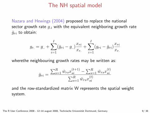
Nazara and Hewings (2004) proposed to replace the nationalsector growth rate g.i with the equivalent neighboring growth rategri to obtain:

gr. = g.. +I∑i=1

(gri − g..)xrixr.

+I∑i=1

(gri − gri)xrixr.

wherethe neighbouring growth rates may be written as:

gri =∑R

s=1 wrsx(t+1)si −

∑Rs=1 wrsx

(t)si∑R

s=1 wrsx(t)si

and the row-standardized matrix W represents the spatial weightsystem.

The R User Conference 2008 - 12–14 august 2008, Technische Universitat Dortmund, Germany 9/ 38

The spatial model for the Italian Register ofBusinesses

The model proposed by Zaccomer (2006, 2007a) for the IRB datauses two decomposition factors: economic activity and enterpriselegal status. This model is based on 6 components:

gr.. = g... + (gr.. − g...) +∑F

f=1(gr.f − gr..)xr.f

xr..

+∑I

i=1(gri. − gr..)xri.xr..

+ Cr +∑I

i=1

∑Ff=1(grif − grif )xrif

xr..

where f identifies the enterprises’ legal status, the component Cris due to the presence of association between the twodecomposition factors and can be written as:

Cr =I∑i=1

F∑f=1

(grif − δrif )xrifxr..

with δrif = gri. + gr.f − gr..The R User Conference 2008 - 12–14 august 2008, Technische Universitat Dortmund, Germany 10/ 38

The components of the IRB model

The growth rate gr.. is then decomposed in

• (1) National component NAZ: the same in the classical model

• (2) Component CFR is related to the gap between theselected unit’s neighbourhood and the national growth rate

• Intra-neighbourhood components: (3) by economic activity;(4) by legal status; (5) Cr (is null in presence of independencebetween industry mix and firm’s legal status).

• (6) National (or regional) component LOC: based on thedifference between unit and neighbouring rates, as in the NHmodel.

The R User Conference 2008 - 12–14 august 2008, Technische Universitat Dortmund, Germany 11/ 38

Spatial weight systems W

There are many methods to construct a spatial weight system. Inthis work, we classify them into three main groups:

G1 based on the physical contiguity of any order (usually thefirst);

G2 distance-based matrices;

G3 based on a territorial reorganization (or “economiccontiguity”).

The R User Conference 2008 - 12–14 august 2008, Technische Universitat Dortmund, Germany 12/ 38

G1: contiguity matrices

The contiguity matrix is a symmetric square binary matrix definedby

wrs ={

1 if s ∈ V (r)0 if s /∈ V (r)

where V (r) is the neighborhood of r-spatial unit. theneighborhood is built on two choices: the first is related to thecriterion (i.g. rook or queen criterion) while the second to thespatial contiguity order.

The R User Conference 2008 - 12–14 august 2008, Technische Universitat Dortmund, Germany 13/ 38

G2: distance-based matrices (1)

• binary matrices with threshold

wrs ={

1 if drs ≤ Dm

0 if drs > Dm

• simple inverse distance

wrs =1dαrs

= d−αrs

• Cliff and Ord (1981) weights

wrs =pβrsdαrs

• negative exponential (with threshold, Stetzer, 1982)

wrs =1

exp(αdrs)= exp(−αdrs)

and

wrs ={

exp(−αdrs) if drs ≤ Dm

0 if drs > DmThe R User Conference 2008 - 12–14 august 2008, Technische Universitat Dortmund, Germany 14/ 38

G2: distance-based matrices (2)

• “economic distances” of Case, Rosen and Hines (1993) andBoarnet (1998) where E is an economic variable (e.g. export)

wrs =1

|Er − Es|and wrs =

1|Er−Es|∑Rs=1

1|Er−Es|

• Molho (1995) and Mitchell, Bill and Juniper (2005)

wrs =Es exp(−αdrs)∑Rh6=r Eh exp(−αdrh)

and

wrs =

{Es exp(−αdrs)PR

h 6=r Eh exp(−αdrh)if drs ≤ Dm

0 if drs > Dm

The R User Conference 2008 - 12–14 august 2008, Technische Universitat Dortmund, Germany 15/ 38

G3: “Economic contiguity”-based W

Zaccomer (2006) proposes a new criterion to build theneighbourhood on a well-known spatial reorganization of themacro-area. This reorganization must be related to the economicphenomenon investigated. For example:

Industrial Districts: neighbourhood ≡ quasi-IDLabour Local Systems: neighbourhood ≡ quasi-LLS

“Quasi” means that the study is based on the usual principle (forW based on the physical contiguity or distance) that a singleterritorial unit is not incorporated in its neighbourhood. Thisimplies that all diagonal elements are wrr = 0.

The R User Conference 2008 - 12–14 august 2008, Technische Universitat Dortmund, Germany 16/ 38

R implementation

The software used to carry out all decompositions, plots and printsfunctions is R.

Firsts steps were developed in Zaccomer and Mason (2007), butnow the R program takes all information directly from the GISsystem and it is not necessary to use the software GeoDa (L.Anselin) for building W matrices.

By now each kind of spatial weight system can be constructed bythis program (i.g. Cliff and Ord).

Finally, physical distances are now calculated on geographiccoordinates of the town hall, and not on the simple polygoncentroid.

The R User Conference 2008 - 12–14 august 2008, Technische Universitat Dortmund, Germany 17/ 38

The code structure

The procedure presents a hierarchical structure of nested microfunctions. The use of the produced routine results is a sequence ofpreliminary actions, the call for the decomposition algorithm and asequence of plot functions.

The R User Conference 2008 - 12–14 august 2008, Technische Universitat Dortmund, Germany 18/ 38

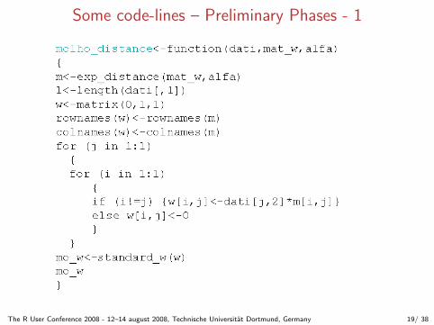
Some code-lines – Preliminary Phases - 1

The R User Conference 2008 - 12–14 august 2008, Technische Universitat Dortmund, Germany 19/ 38

Some code-lines – Preliminary Phases - 2

The R User Conference 2008 - 12–14 august 2008, Technische Universitat Dortmund, Germany 20/ 38

Some code-lines – The SSS Decomposition - 1

The R User Conference 2008 - 12–14 august 2008, Technische Universitat Dortmund, Germany 21/ 38

Some code-lines – The SSS Decomposition - 2

The R User Conference 2008 - 12–14 august 2008, Technische Universitat Dortmund, Germany 22/ 38

Some code-lines – The SSS Decomposition - 3

The R User Conference 2008 - 12–14 august 2008, Technische Universitat Dortmund, Germany 23/ 38

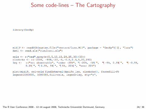
Some code-lines – The Cartography

The R User Conference 2008 - 12–14 august 2008, Technische Universitat Dortmund, Germany 24/ 38

Empirical results

The application was carried out on regional industrial employmentdata for 2001-04. These refer to the Italian Business StatisticalRegister (ASIA) for 214 municipalities (LAU2 level) and 5municipalities are omitted because they do not present anymanufacturing enterprise.

The dataset structure counts:

• 12 LLS of the FVG (NUTS2 level)

• 10 manufacturing sectors are obtained from NACE Rev. 1.1[The enterprises entering sector D are grouped in 10 clusters.]

• 3 legal statusI soleI limitedI unlimited

The R User Conference 2008 - 12–14 august 2008, Technische Universitat Dortmund, Germany 25/ 38

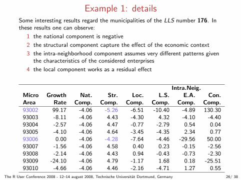
Example 1: detailsSome interesting results regard the municipalities of the LLS number 176. Inthese results one can observe:

1 the national component is negative

2 the structural component capture the effect of the economic context

3 the intra-neighborhood component assumes very different patterns giventhe characteristics of the considered enterprises

4 the local component works as a residual effect

Intra.Neig.Micro Growth Nat. Str. Loc. L.S. E.A. Con.Area Rate Comp. Comp. Comp. Comp. Comp. Comp.93002 99.17 -4.06 -5.26 -6.51 -10.40 -4.89 130.3093003 -8.11 -4.06 4.43 -4.30 4.32 -4.10 -4.4093004 -2.57 -4.06 4.47 -0.77 -2.79 0.54 0.0493005 -4.10 -4.06 4.64 -3.45 -4.35 2.34 0.7793006 0.00 -4.06 -4.28 -7.64 -4.46 -29.56 50.0093007 -1.56 -4.06 4.58 0.40 0.23 -0.15 -2.5693008 -2.14 -4.06 4.43 0.94 -0.43 -0.73 -2.3093009 -24.10 -4.06 4.79 -1.17 1.68 0.18 -25.5193010 -4.66 -4.06 4.46 -2.16 -4.71 1.27 0.55

The R User Conference 2008 - 12–14 august 2008, Technische Universitat Dortmund, Germany 26/ 38

Example 1: cartography - growth rates

not observableover 20%[5%, 20%][0.5%, 5%[[−0.5%, 0.5%[[−5%, −0.5%[[−20%, −5%[under −20%

N

10 km

The R User Conference 2008 - 12–14 august 2008, Technische Universitat Dortmund, Germany 27/ 38

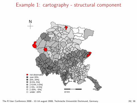
Example 1: cartography - structural component

not observableover 20%[5%, 20%][0.5%, 5%[[−0.5%, 0.5%[[−5%, −0.5%[[−20%, −5%[under −20%

N

10 km

The R User Conference 2008 - 12–14 august 2008, Technische Universitat Dortmund, Germany 28/ 38

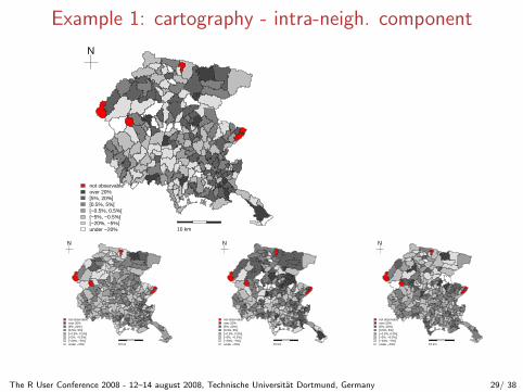
Example 1: cartography - intra-neigh. component

not observableover 20%[5%, 20%][0.5%, 5%[[−0.5%, 0.5%[[−5%, −0.5%[[−20%, −5%[under −20%

N

10 km

not observableover 20%[5%, 20%][0.5%, 5%[[−0.5%, 0.5%[[−5%, −0.5%[[−20%, −5%[under −20%

N

10 km

not observableover 20%[5%, 20%][0.5%, 5%[[−0.5%, 0.5%[[−5%, −0.5%[[−20%, −5%[under −20%

N

10 km

not observableover 20%[5%, 20%][0.5%, 5%[[−0.5%, 0.5%[[−5%, −0.5%[[−20%, −5%[under −20%

N

10 km

The R User Conference 2008 - 12–14 august 2008, Technische Universitat Dortmund, Germany 29/ 38

Example 1: cartography - local component

not observableover 20%[5%, 20%][0.5%, 5%[[−0.5%, 0.5%[[−5%, −0.5%[[−20%, −5%[under −20%

N

10 km

The R User Conference 2008 - 12–14 august 2008, Technische Universitat Dortmund, Germany 30/ 38

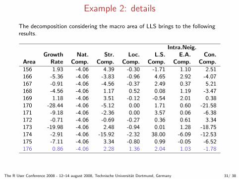
Example 2: details

The decomposition considering the macro area of LLS brings to the followingresults.

Intra.Neig.Growth Nat. Str. Loc. L.S. E.A. Con.

Area Rate Comp. Comp. Comp. Comp. Comp. Comp.156 1.93 -4.06 4.39 -0.30 -1.71 1.10 2.51166 -5.36 -4.06 -3.83 -0.96 4.65 2.92 -4.07167 -0.91 -4.06 -4.56 -0.37 2.49 0.37 5.21168 -4.56 -4.06 1.17 0.52 0.08 1.19 -3.47169 1.18 -4.06 3.51 -0.12 -0.54 2.01 0.38170 -28.44 -4.06 -5.12 0.00 1.71 0.60 -21.58171 -9.18 -4.06 -2.36 0.00 3.57 0.06 -6.38172 -0.71 -4.06 -0.69 -0.27 0.36 0.61 3.34173 -19.98 -4.06 2.48 -0.94 0.01 1.28 -18.75174 -2.91 -4.06 -15.92 -2.32 38.00 -6.09 -12.53175 -7.11 -4.06 3.34 -0.80 0.99 -0.05 -6.52176 0.86 -4.06 2.28 1.36 2.04 1.03 -1.78

The R User Conference 2008 - 12–14 august 2008, Technische Universitat Dortmund, Germany 31/ 38

Detailed cartography - growth rates

not observableover 20%[5%, 20%][0.5%, 5%[[−0.5%, 0.5%[[−5%, −0.5%[[−20%, −5%[under −20%

The R User Conference 2008 - 12–14 august 2008, Technische Universitat Dortmund, Germany 32/ 38

Detailed cartography - structural component

not observableover 20%[5%, 20%][0.5%, 5%[[−0.5%, 0.5%[[−5%, −0.5%[[−20%, −5%[under −20%

The R User Conference 2008 - 12–14 august 2008, Technische Universitat Dortmund, Germany 33/ 38

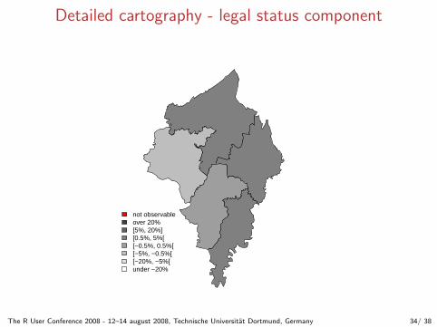
Detailed cartography - legal status component

not observableover 20%[5%, 20%][0.5%, 5%[[−0.5%, 0.5%[[−5%, −0.5%[[−20%, −5%[under −20%

The R User Conference 2008 - 12–14 august 2008, Technische Universitat Dortmund, Germany 34/ 38

Detailed cartography - econ.act. component

not observableover 20%[5%, 20%][0.5%, 5%[[−0.5%, 0.5%[[−5%, −0.5%[[−20%, −5%[under −20%

The R User Conference 2008 - 12–14 august 2008, Technische Universitat Dortmund, Germany 35/ 38

Detailed cartography - connection component

not observableover 20%[5%, 20%][0.5%, 5%[[−0.5%, 0.5%[[−5%, −0.5%[[−20%, −5%[under −20%

The R User Conference 2008 - 12–14 august 2008, Technische Universitat Dortmund, Germany 36/ 38

Detailed cartography - local component

not observableover 20%[5%, 20%][0.5%, 5%[[−0.5%, 0.5%[[−5%, −0.5%[[−20%, −5%[under −20%

The R User Conference 2008 - 12–14 august 2008, Technische Universitat Dortmund, Germany 37/ 38

Concluding remarks and ongoing

Till now we developed

• a full 6 component shift-share decomposition

• the code for data reorganization and preliminary analysis

• the distance calculation (considering all possible distances)

• an integrated cartography adopting the package “GeoXp” andall correlated packages.

And now its time for

• some necessary code refinement

The R User Conference 2008 - 12–14 august 2008, Technische Universitat Dortmund, Germany 38/ 38