Utility of stochastic decadal simulations in water resource planning

Arthur M. Greene, Lisa Goddard, Paula Gonzalez

International Research Institute for Climate and Society (IRI)

Columbia University, New York, NY USA

GloDecH, May 11, 2011

•  Skillful decadal forecasts, particularly at regional scales (and over land), still lie in the future.

•  A potentially useful alternative: Synthetic data sequences, conditioned by observations and including a regional climate change component.

•  Some considerations in simulation design. •  Case Study: Berg River, Western Cape

province, South Africa.

In a nutshell…

State-of-the-art initialized precipitation forecasts

Data courtesy Doug Smith (see Smith et al., Science 2007)

r

RMSE

Verification: Average of 2-5 yr lead forecasts for annual mean precipitation, using GPCC.

No improvement over unitialized forecasts in southernmost Africa.

Case study: Berg river watershed, W. Cape Province, S. Africa

• Length: ~300km

• Catchment: 7715 km2

• Headwaters in the Drakenstein Mts., ~1000 m.a.s.l.

• precip, temperature gradients with elevation

• Principal H2O source for Cape Town, including commercial, industrial

• Economically significant agricultural resource

• Extant hydrology, economic models

• Availability of data, models provides an excellent testbed

•  Projection of regional climate change –  Estimation of regional response –  Implicit role for IPCC models

•  Identification of systematic signal components –  Here, meaning “significantly different from AR(1)” –  A key decision: How to represent? One option: “WARM”

•  Stationarity assumptions –  Second moments –  Serial autocorrelation ( AR(1) variability) –  Seasonal cycle, daily statistics –  Local/regional covariation – spatial scale of decadal “footprint”

•  Description of uncertainty –  Arises at many levels: intermodel, scenario, estimation… –  Not solely a matter of amplitude, but also temporal behavior

•  Multivariate model –  May be required by downstream modeling framework –  Best if training data conforms…

Simulation design issues

Simulation schematic

Green arrows: Operator judgment required. Cannot be a “black box.”

•  p-value for rejecting H0: Residuals are not lag-1 autocorrelated.

•  Regression is on the MMM global mean temperature.

•  Annual mean precip (top), temperature (below).

•  NOT screened for filled data…

Where is redness?

•  Multivariate setting: pr, Tmax, Tmin •  Obs: 50 yr of daily data (1950-1999) for 171 quinary

catchments in the Berg (mostly) and Breede WMAs. •  Forced trends from IPCC (A1B)

- For Tmax, Tmin, via 20C regression - For pr, via 21C regression

•  No evidence for systematic low-frequency variation: Incorporate trend + stochastic components only.

•  Precipitation essentially white; temperature exhibits some lag-1 autocorrelation.

•  Low-frequency (annual–multidecadal) variability simulated with VAR(1) model.

•  Subannual variations generated by “block resampling” of observations.

Simulation overview

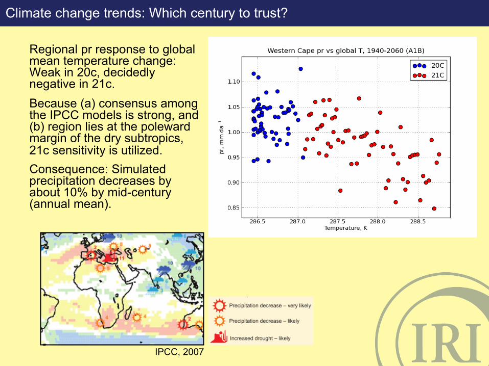
Regional pr response to global mean temperature change: Weak in 20c, decidedly negative in 21c. Because (a) consensus among the IPCC models is strong, and (b) region lies at the poleward margin of the dry subtropics, 21c sensitivity is utilized. Consequence: Simulated precipitation decreases by about 10% by mid-century (annual mean).

Climate change trends: Which century to trust?

IPCC, 2007

•  A regular oscillation with 18-yr period has been reported for precipitation in Southern Africa. Wavelet analysis of the 171-catchment mean (right) does not indicate the presence of such a signal. The catchment mean is used here as the simulation target.

•  Simulations will then comprise just two components: Climate change trend and stochastic variations. These elements are treated independently, then combined.

What’s the frequency, Kenneth?

Vector autoregressive (VAR) model in brief

Formally, , where yt is a three-component vector (pr, Tmax, Tmin) at time t,

A is a (3 x 3) matrix of coefficients,

yt-1 is the same vector one time step (year) previous,

et is a white-noise process with covariance matrix , which may have nonzero off-diagonal elements.

•  Historically, VAR models have been associated more with econometrics than climate, where “linear inverse models” (LIMs) have seen considerable deployment. Structurally, VAR(1) and LIM appear to be identical.

•  For our purposes, two data characteristics are of primary concern: Intervariable correlation, and serial autocorrelation in the individual variables.

Σ

yt=Ay

t!1 + et

Intervariable correlation

Observations pr Tmax Tmin pr 1.000 Tmax -0.447 1.000 Tmin 0.068 0.733 1.000 Simulation pr Tmax Tmin pr 1.000 Tmax -0.445 1.000 Tmin 0.068 0.733 1.000

VAR and simulation statistics

Annualized data (171-station means)

Serial autocorrelation

pr Tmax Tmin

Obs 0.004 0.168 0.297 Sim -0.008 0.176 0.303 Tmin significant at 0.05, Tmax not quite…

•  Individual station records are well-correlated with the “regional” signal: Catchment behaves coherently (top).

•  Downscaled to station level via linear regression.

•  Subannual variations taken from randomly resampled sequence of years in the observations, providing spatial coherence.

•  Simulation can be propagated to a single station (bottom), a subset or the entire catchment, in the latter case producing a distributed streamflow scenario.

•  Large ensemble of simulations permits precise specification of desired characteristics, useful for well-defined follow-on model experiments.

Propagation of simulations to the local level Station correlations with regional signal

Station-level simulation; T trends are local

Some concluding thoughts…

•  Method can be thought of as a “decadal weather generator” incorporating a climate change component.

•  For the random component a VAR(1) model is utilized; Given the potential variety of regional behaviors and available data, other models may also prove relevant.

•  Changepoints, “abrupt” behavior not evident in the observational record; no provision made for these in simulations.

•  Uncertainty owing to differences in model formulation not treated. •  Relevant paleodata can augment the instrumental record. •  Simulations are presently being run in the first “downstream” (hydrology) model: Agricultural Catchments Research Unit (ACRU), University of Natal. Stay tuned!

-~- The End -~- amg@iri.columbia.edu