utilizing shadow prices in the ontario electricity market · pdf fileutilizing shadow prices...

Utilizing Shadow Prices In the Ontario Electricity Market


July 20, 2007

Contents Introduction ................................................................................................................................................... 1

Background ................................................................................................................................................... 2

Bids and Offers ............................................................................................................................................. 3

Maximizing the Gain from Trade ................................................................................................................. 4

Market Prices vs. Shadow Prices .................................................................................................................. 5

Joint Optimization ......................................................................................................................................... 7

Ramp-Rate Constraints ............................................................................................................................... 10

Reserve Loading Point ................................................................................................................................ 13

Resource Dispatch Filter ............................................................................................................................. 13

Steps in Reverse-Engineering Shadow Prices ............................................................................................ 14

Reverse-Engineering Step 1 – Constrained Dispatch Calculations ..................................................... 15

Reverse-Engineering Step 2 – Market Schedule Calculations ............................................................ 16

Reverse-Engineering Step 3 – Settlements and CMSC Calculations .................................................. 17

Sygration Generation Market Simulator ..................................................................................................... 18

Author ......................................................................................................................................................... 21

References ................................................................................................................................................... 21

Introduction

Shadow prices are generated by the Independent Electricity System Operator (IESO) market systems for

most nodes on the Ontario transmission system. They are published for energy and three classes of

operating reserve for every 5-minute interval. However, since they are not used for any settlements

calculations their value to dispatchable participants is often overlooked.

This document focuses on a generator’s role in the electricity market, and explains how energy offers,

operating reserve offers and shadow prices can be used to determine a generator’s dispatch instructions.

This would be useful to new generators wishing to develop a first-time bidding strategy, or to existing

generators wishing to fine-tune their offers in order to improve their operational efficiencies through more

desirable dispatches. It can also be used by non-dispatchable generators that are considering becoming


dispatchable in order to have their production coincide better with higher energy prices and to enter the

operating reserve market. A technique is shown that uses joint optimization to determine dispatch

quantities, market schedules and settlements credits using the historical shadow price data. Finally, the

Sygration Generation Market Simulator service is introduced as a commercial alternative to parties

considering implementing these techniques in-house.

This document is intended for readers that are familiar with the Ontario electricity market and have

dispatchable generators, or are considering becoming dispatchable.

Background

The Ontario wholesale electricity market uses a uniform market price for wholesale purchases and sales

of electricity. The wholesale price to distributors and participants that are not dispatched by the IESO is

based on the average Hourly Ontario energy price (HOEP), while the price to generators and large

industrial customers that are dispatched by the IESO is the 5-minute Market Clearing Price (MCP) 1. In

both cases, this wholesale market price is always the same for all locations throughout the province and

does not truly reflect the effects of such things as transmission losses, congestion and actual generator

ramping limitations. This was the intention of the original designers of the Ontario electricity market and

they used the postage stamp analogy where everyone pays the same price to send a letter anywhere in the

country. It is referred to as the Unconstrained Market Model, and is used to determine the market prices

by ignoring many real-life transmission system constraints or inflating unit ramping capabilities.

System constraints cannot be ignored when it comes to operating the electricity system, including the

dispatch of generators or large industrial loads (dispatchable). Not only does this result in a safer

operation of the transmission system (by keeping transmission flows within safe limits), it also results in a

more efficient energy exchange by factoring in transmission losses. The dispatch of electricity is based

on the Constrained Model that recognizes the impact of:

Transmission losses

Transmission operating limits

Resource ramping capabilities

Limits placed on how much operating reserve can come from specific areas of the grid

Multi-interval optimization that looks ahead at changes in supply and demand

Of course, both the Constrained Model and Unconstrained Market Model operate on the bids and offers

for energy and operating reserve that are submitted by generators and dispatchable consumers. Every five

minutes, the IESO’s Dispatch Scheduler and Optimizer balances these bids and offers along with the

current and forecast demand to arrive at individual market schedules (using the Unconstrained Market

Model) and dispatch instructions (using the Constrained Model). The constrained model runs first and

uses the most recent demand predictions in determining the dispatches for the interval, while the

unconstrained run actually runs after the interval and uses actual demand and supply values sample during

the interval. The end of both processes is the creation of a single set of market prices for the entire

province and the 13 intertie zones, as well as individual shadow prices for most major connections

(“nodes”) to the system.

1 The final price for energy may actually regulated for some users, or include global adjustments, uplifts and tariffs. All of these

are beyond the scope of this document.


Market prices are important because they are used as the basis of energy and operating reserve

settlements. However, the shadow prices tell where there is a greater or lesser need for energy, as well as

how generators and consumers are being dispatched throughout the province. Shadow prices can also be

used to work backwards from trial bids and offers to determine how a unit would have been dispatched

had these bids been used for real.

Bids and Offers

Dispatchable participants submit bids to buy or offers to sell energy to the IESO for every hour of the day.

If they are capable (and authorized) to sell operating reserve, they may optionally submit offers for

operating reserve2 for the same hours. For generators, these offers are assumed to represent their cost to

produce energy, or in the case of operating reserve their cost to be on stand-by to provide energy upon

short notice. The Ontario market employs a Dispatch Scheduler and Optimizer (DSO) which evaluates all

of the bids and offers for both energy and the three classes of operating reserve simultaneously in a

process called Joint Optimization. The market schedules and dispatches produced by the DSO balances

the demand and supply for both energy and operating reserve, with the objective of maximizing the

economic gain to both individual generators and consumers.

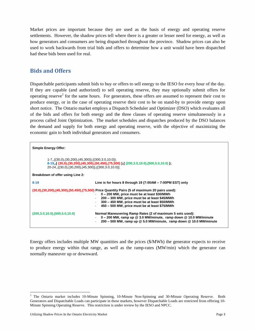
Simple Energy Offer:

1-7,,{(30,0),(30,200),(45,300)},{(300,3.0,10.0)}; 8-19,,{ (30,0),(30,200),(45,300),(50,450),(75,500) },{ (200,3.0,10.0),(500,5.0,10.0) }; 20-24,,{(30,0),(30,200),(45,300)},{(300,3.0,10.0)};

Breakdown of offer using Line 2: 8-19 Line is for hours 8 through 19 (7:00AM – 7:00PM EST) only (30,0),(30,200),(45,300),(50,450),(75,500) Price Quantity Pairs (5 of maximum 20 pairs used):

- 0 – 200 MW, price must be at least $30/MWh - 200 – 300 MW, price must be at least $45/MWh - 300 – 450 MW, price must be at least $50/MWh - 450 – 500 MW, price must be at least $75/MWh

(200,3.0,10.0),(500,5.0,10.0) Normal Maneuvering Ramp Rates (2 of maximum 5 sets used):

- 0 – 200 MW, ramp up @ 3.0 MW/minute, ramp down @ 10.0 MW/minute

- 200 – 500 MW, ramp up @ 5.0 MW/minute, ramp down @ 10.0 MW/minute

Energy offers includes multiple MW quantities and the prices ($/MWh) the generator expects to receive

to produce energy within that range, as well as the ramp-rates (MW/min) which the generator can

normally maneuver up or downward.

2 The Ontario market includes 10-Minute Spinning, 10-Minute Non-Spinning and 30-Minute Operating Reserve. Both

Generators and Dispatchable Loads can participate in these markets, however Dispatchable Loads are restricted from offering 10-

Minute Spinning Operating Reserve. This restriction is under review by the IESO and NPCC.


Maximizing the Gain from Trade

In balancing the supply and demand for electricity every 5 minutes the DSO selects the quantities of

energy and operating reserve from each bid and offer in such a way that the cost to the market is optimal

– the prices are just enough and not any more or less than they need to be to satisfy both buyers and

sellers. This is said to result in a maximizing the economic gain from trade, where the common price for

electricity allows generators to produce and consumers to consume with an optimal operating profit.

To a generator, this operating profit is determined by their electricity revenue (Market Price x MWh) less

their production costs. Since their energy and operating reserve offers are assumed to represent their

production costs, the operating profit can be calculated as the area between the price and their offer, up to

the scheduled quantity. See examples 1 through 3 for an illustration of this. In the simple case where a

generator is only offering energy, the quantity scheduled by the DSO would only include offered

quantities at or below the market price. At that market price, if a lesser quantity was scheduled it would

not be optimal to the generator as it was willing to sell more energy for a greater profit. It would also be

non-optimal to the market since it would be holding back energy from loads that were willing to consume

more at that price. A key concept here is that such optimization occurs at both the market level and at the

individual resource level. While dispatch quantities and prices are the consequence of the joint

optimization process, these historical prices can also be applied against the offers to determine the

expected dispatch quantities.

Calculating Economic Gain:

The price-quantity pairs of the generator’s offer can be shown as laminations on a bar chart. Since these offers represent the cost

of energy production for generators, the economic gain or operating profit is the difference between the market price and the

offer prices up to the scheduled quantity.

Example 1: Market Price = $47.00

Using the simple energy offer above for hours 8-19: an energy price of $47 would result in a schedule of 300MW and an

operating profit of $3,600/MWh (yellow area). Any quantity higher or lower than 300MW would result in a reduction of

operating profit (not maximized). This leaves an additional 200MW of energy unscheduled.

0 200 300 450 500 MW

$75

$50

$45

$30

Market Price $47.00

Operating Profit = $3,600 / MWh

($47 - $30) x 200 +

($47 - $45) x 100

Market Schedule: 300 MW


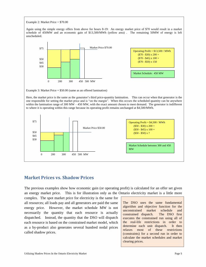
Example 2: Market Price = $70.00

Again using the simple energy offers from above for hours 8-19: An energy market price of $70 would result in a market

schedule of 450MW and an economic gain of $13,500/MWh (yellow area) . The remaining 50MW of energy is left

unscheduled.

Example 3: Market Price = $50.00 (same as an offered lamination)

Here, the market price is the same as the generator’s third price-quantity lamination. This can occur when that generator is the

one responsible for setting the market price and is “on the margin”. When this occurs the scheduled quantity can be anywhere

within the lamination range of 300 MW – 450 MW, with the exact amount chosen to meet demand. The generator is indifferent

to where it is operating within this range because its operating profit remains unchanged at $4,500/MWh.

Market Prices vs. Shadow Prices

The previous examples show how economic gain (or operating profit) is calculated for an offer set given

an energy market price. This is for illustration only as the Ontario electricity market is a little more

complex. The spot market price for electricity is the same for

all resources; all loads pay and all generators are paid the same

energy price. However, the market schedule MW is not

necessarily the quantity that each resource is actually

dispatched. Instead, the quantity that the DSO will dispatch

each resource is based on the constrained market model, which

as a by-product also generates several hundred nodal prices

called shadow prices.

The DSO uses the same fundamental

algorithm and objective function for the

unconstrained market schedule and

constrained dispatch. The DSO first

executes the constrained run using all of

the real-life restrictions in order to

determine each unit dispatch. It then

relaxes most of these restrictions

(constraints) for a second run in order to

calculate the market schedules and market

clearing prices.

0 200 300 450 500 MW

$75

$50

$45

$30

Market Price $70.00


($70 - $30) x 200 +

($70 - $45) x 100 +

($70 - $50) x 150

Market Schedule: 450 MW


($50 - $30) x 200 +

($50 - $45) x 100 +

($50 - $50) x ?

Market Schedule between 300 and 450

MW

0 200 300 450 500 MW

$75

$50

$45

$30

Market Price $50.00


The shadow prices at each node are consistent with the actual dispatch quantity of any resource at that

node. That is to say, given a set of offers and a set of shadow prices you can determine the dispatch

quantity in the same manner as in examples 1 – 3. The calculation of operating profit using shadow

prices is still valid in establishing the dispatch quantities, however, it is not used directly in any

settlements calculations. No payments are based on shadow prices. Instead, the market price is used on

three occasions to determine three operating profit calculations based on 1) the market schedule quantity,

2) the constrained dispatch quantity and 3) the quantity that was actually provided (using revenue

metering data). A Congestion Management Settlement Credit (CMSC) is an adjustment calculated by the

IESO Settlements system to ensure the operating profit for each interval is kept true to the operating profit

that would have been received based on the market schedule.

CMSC = OP Market Schedule – MAX(OP Dispatch Quantity , OP Actual Quantity)

Since the adjustment uses the maximum of the Operating Profits based on Dispatch Quantity and Actual

Quantity, this effectively claws-back any Operating Profit the participant might have received by over-

generating. The CMSC is effectively a constrained-on or constrained-off payment, and is an incentive to

the participant to follow the constrained dispatch instructions. It is calculated separately for Energy and

each class of Operating Reserve and can be a negative value.

CMSC Calculation:

The energy offer is shown twice, first with the Market Price and then with the Shadow Price. Each price would result in a

different energy quantity for the market schedule and the constrained dispatch. The energy Shadow Price is lower than the

Market Price, indicating that there may be an oversupply of energy in the area resulting in the need to constrain down generation

or constrain up loads.

Market Price $70.00

0 200 300 450 500 MW

$75

$50

$45

$30

Market Schedule 450 MW

0 200 300 450 500 MW

$75

$50

$45

$30

Shadow Price $48.00

Constrained Dispatch 300 MW


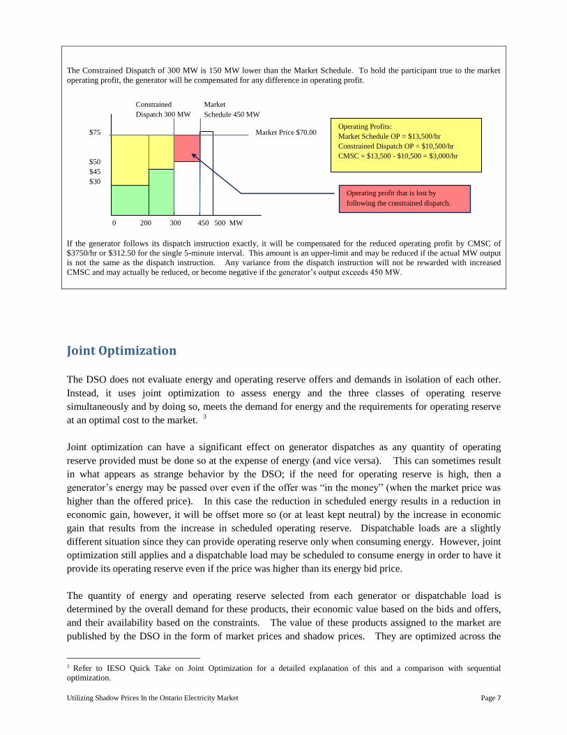
The Constrained Dispatch of 300 MW is 150 MW lower than the Market Schedule. To hold the participant true to the market

operating profit, the generator will be compensated for any difference in operating profit.

If the generator follows its dispatch instruction exactly, it will be compensated for the reduced operating profit by CMSC of

$3750/hr or $312.50 for the single 5-minute interval. This amount is an upper-limit and may be reduced if the actual MW output

is not the same as the dispatch instruction. Any variance from the dispatch instruction will not be rewarded with increased

CMSC and may actually be reduced, or become negative if the generator’s output exceeds 450 MW.

Joint Optimization

The DSO does not evaluate energy and operating reserve offers and demands in isolation of each other.

Instead, it uses joint optimization to assess energy and the three classes of operating reserve

simultaneously and by doing so, meets the demand for energy and the requirements for operating reserve

at an optimal cost to the market. 3

Joint optimization can have a significant effect on generator dispatches as any quantity of operating

reserve provided must be done so at the expense of energy (and vice versa). This can sometimes result

in what appears as strange behavior by the DSO; if the need for operating reserve is high, then a

generator’s energy may be passed over even if the offer was “in the money” (when the market price was

higher than the offered price). In this case the reduction in scheduled energy results in a reduction in

economic gain, however, it will be offset more so (or at least kept neutral) by the increase in economic

gain that results from the increase in scheduled operating reserve. Dispatchable loads are a slightly

different situation since they can provide operating reserve only when consuming energy. However, joint

optimization still applies and a dispatchable load may be scheduled to consume energy in order to have it

provide its operating reserve even if the price was higher than its energy bid price.

The quantity of energy and operating reserve selected from each generator or dispatchable load is

determined by the overall demand for these products, their economic value based on the bids and offers,

and their availability based on the constraints. The value of these products assigned to the market are

published by the DSO in the form of market prices and shadow prices. They are optimized across the

3 Refer to IESO Quick Take on Joint Optimization for a detailed explanation of this and a comparison with sequential

optimization.

Operating Profits:

Market Schedule OP = $13,500/hr

Constrained Dispatch OP = $10,500/hr

CMSC = $13,500 - $10,500 = $3,000/hr

0 200 300 450 500 MW

$75

$50

$45

$30

Market

Schedule 450 MW

Constrained

Dispatch 300 MW

Market Price $70.00

Operating profit that is lost by

following the constrained dispatch.


market as a whole, meaning the price is not unnecessarily high or low in order to meet the supply and

demand for energy and operating reserve. They are also optimized across each individual unit’s offer set,

meaning the MW quantities scheduled or dispatched for a generator will result in the maximum quantity

at that price considering the economic gain of both energy and operating reserve.

Example 4A shows how Joint Optimization is applied using an energy offer and operating reserve offer.

You can see in the example that the energy market price was higher than the generator’s energy offer

price for a significant portion, yet the quantity was still not scheduled. It might appear at first glance that

the DSO made an error by passing over the quantity of energy that had a positive economic gain. A

closer look shows that it did this so it could schedule some operating reserve and the overall selection

resulted in an even higher economic gain. Example 4B shows how these quantities were assessed and

chosen.

Example 4A: Joint Optimization

Market Prices: Energy $55/MWh, 10-Min Non-Spin OR $20/MWh, 30-Min OR $5/MWh

The earlier energy offer for hours 8-19 is used here. However, additional offers for 10-Minute Non-Spinning Operating Reserve

and 30-Minute Operating Reserve have also been submitted. Even though individual offer quantities appear to be “in the money”,

not all quantities are scheduled. Instead, the joint optimization finds that maximum economic gain occurs through scheduling a

mix of energy and operating reserve:

Energy: 300 MW Scheduled

10-Minute Spinning OR: 100 MW Scheduled

30-Minute OR: 100 MW Scheduled

Energy Offer / Schedule

10-Minute Non-Spinning Operating Reserve

Market Price $55.00. Scheduled Quantity 300 MW

Market Price $15.00 Scheduled Quantity 100 MW

Economic Gain:

0 – 200 MW $25.00/MWh √ scheduled


300 – 450 MW $5.00/MWh X not scheduled

450 – 500 MW -$20.00/MWh X not scheduled

Economic Gain:


100– 300 MW $6.50/MWh X not scheduled


0 200 300 450 500 MW

simple energy offer above for hours 8-19:

an energy price of $47 would result in a

schedule of 300MW and an economic gain

of $3,600/MWh (yellow area). This leaves

an additional 200MW of energy

unscheduled.

500 MW

$75

$50

$45

$30

The energy offer of range 300 – 450MW @ $50/MWh

appeared “in the money” but was not chosen because

its economic gain would be less than either operating

reserve offers.

0 100 300 500 MW

simple energy offer above for hours 8-

19: an energy price of $47 would result

in a schedule of 300MW and an

economic gain of $3,600/MWh (yellow

area). This leaves an additional

$20.00

$8.50

$5.50


30-Minute Operating Reserve

3

To show how the various quantities of energy and operating reserve were scheduled, determine how much

operating profit each lamination quantity would contribute. These operating profit laminations can then

be sorted from highest to lowest $/MWh to establish their economic priority. Sum up the total quantities

from left to right that 1) result in an increase in operating profit as the laminations are positive, and 2) are

at or below the maximum energy offered within the hour.

Example 4B: Operating Profit Laminations

Using the offers and prices shown in Example 4A, we can order the Operating Profit laminations from highest to lowest to

determine what quantities from energy and operating reserve would result in the greatest operating profit.

0 100 200 300 500 MW

simple energy offer above for hours 8-19: an

energy price of $47 would result in a schedule

of 300MW and an economic gain of

$3,600/MWh (yellow area). This leaves an

additional 200MW of energy unscheduled.

500 MW

Market Price $7.00 Scheduled Quantity 100 MW

$10.00

$3.00

$1.00

$0.00

Economic Gain:


100– 200 MW $6.00/MWh X not scheduled

200 – 300 MW $4.00/MWh X not scheduled


Scheduled Not Scheduled

(Beyond Max Energy)

Not Scheduled

(Decreasing Benefit)

$25

$20

$15

$10

$5

$0

-$5

-$10

-$15

-$20

ENERGY

OR 10 NON-SPIN

OR 30 MINUTE

The total scheduled quantity of energy and operating

reserve must never exceed the maximum energy

offered during the hour. While economic laminations

may still remain, only the quantities up to 500 MW

will be scheduled.

Operating Profit Lamination Legend:

100 200 300 400 500 600 700 800 900 1000 1200 1400 1500

simple energy offer above for hours 8-19: an energy price of $47 would result in a schedule

of 300MW and an economic gain of $3,600/MWh (yellow area). This leaves an additional

200MW of energy unscheduled.

500 MW


Ramp-Rate Constraints

Ramp-rates are submitted by participants within their energy offers and tell the IESO how each resource

can maneuver under normal operating conditions. Dispatch instructions sent to the participant will follow

these ramp-rates to ensure the technical operating limits of the units are respected. A separate operating

reserve ramp-rate is also submitted by the participant to indicate how quickly a unit can increase its

energy under short notice in response to unexpected outages, demand or other contingencies. The

previous examples ignored the effect of ramp rates on the joint optimization and assumed that all energy

and operating reserve was available for the interval. In reality, the DSO constantly tracks where the

resource is currently operating and factors in the ramp-rates to establish upper and lower energy

boundaries for the next 5-minute interval. Similarly, the operating reserve ramp-rate (provided separately

in the energy bid/offer) is used to establish a maximum upper boundary for 10-minute and 30-minute

operating reserve. Regardless of how much of the offer is in the money, a unit’s next dispatch will

always be within this range.

Submitted Ramp Rates: (200,3.0,10.0),(500,5.0,10.0)

Current Output 200MW

Minimum Constrained Dispatch = 200 MW – 3.0 MW/min x 5 minutes = 185 MW

Maximum Dispatch = 200 MW + 10.0 MW/min x 5 minutes = 250 MW

The DSO handles energy ramp rates differently for the constrained dispatch and market schedule. While

the constrained dispatch respects the ramp rates at face value, the market schedule currently uses a

multiplier of 12 times ramp-rate4 when calculating the upper and lower energy boundaries. In this

example the market schedule would be ramp-rate limited between 20 MW (200 – 3 x 5 x 12) and 800

MW (200 + 10 x 5 x 12) for the next 5-minute interval.

If a resource will be participating in the operating reserve market, a separate operating reserve ramp rate

is also provided (within the energy bid body) for use with all operating reserve offers. This ramp-rate

indicates the MW/minute rate a unit can increase its energy output should operating reserve be activated.

4 In early 2007, the IESO Board of Directors proposed changing the 12-times ramp rate in the market schedule to 3-times. This

was challenged by the Association of Major Power Consumers of Ontario (AMPCO) to the Ontario Energy Board, but was

denied. AMPCO has since filed an appeal in the Superior Court of Justice, Divisional Court [Source: Stikeman Elliott LLP].

Next dispatch interval is ramp-rate constrained to between 185 MW and 250 MW

0 200 300 450 500 MW

$75

$50

$45

$30

Current output

200MW


For establishing the maximum operating reserve allowed, the DSO multiplies this ramp-rate by either 10

minutes (for 10-Minute spinning and non-spinning operating reserve) or 30 minutes (for 30-minute

operating reserve). Unlike the energy ramp-rates, the DSO does not implement any multiplier in

determining the maximum operating reserve for the unconstrained market schedule.

In example 4B, the operating profit laminations for energy and operating reserve were determined then

sorted from highest to lowest $/MWh. It treated each of these laminations as being optional where the

quantities would be chosen if they resulted in a positive additional operating profit, up the maximum

energy offered. Because of the ramp-rates, two things happen for each interval. First, portions of the

laminations may have to be discarded if the energy or operating reserve cannot be reached during the

target timeframe (5-minute energy, 10-minute OR or 30-minute OR). Second, portions of the energy

laminations may be mandatory and must be scheduled regardless if they result in positive or negative

operating profit, if the unit cannot ramp down energy quickly enough to achieve 0 MW output.

The trajectory calculations above assume that a unit has been following its dispatch instructions to get to

its current output. In spring 2004 the IESO implemented a feature of their Multi-Interval Optimization

project to continually track how well certain units (some non-quick start generators) were following their

dispatch instructions. Logic was added to the DSO to accelerate the ramp-rate when a unit is falls behind

their dispatch instructions when loading up. This was done in order to reduce or eliminate the “Stutter

Step” by allowing these units to catch up to their target output levels when they momentarily fall behind.

Refer to IESO Quick Take Issue 13 for a full explanation.

Energy Offer Laminations evaluated for Constrained Dispatch:

Current Output 200 MW. Ramp-rates limit next interval to between 185 MW and 250 MW

0-185 MW lamination becomes mandatory. 185-250 MW will be assessed on merit. Above 250 MW must be discarded.

0 200 300 450 500 MW

Mandatory Discard

Assessed on Merit

$75

$50

$45

$30

Current output

200MW


Example 4C: Including Ramp-Rate Constraints

Current Energy Output: 200 MW

Operating Reserve Ramp-Rate: 10 MW/minute

As a result of energy and operating reserve ramp-rate constraints on the next 5-minute interval, the first 185MW of energy

becomes mandatory. Energy laminations above 250MW becomes discarded, as does 10-Minute Spinning OR above 100MW and

30-Minute OR above 300 MW. Remaining laminations are shifted to the left for further consideration.

Totaling up the laminations, the final dispatch will be Energy 250MW, OR 10-Minute Non-Spin 100 MW and OR 30-Minute

150 MW.

Hourly Pre-dispatch Shadow Prices

Pre-dispatch Shadow Prices for each delivery point are also published hourly with data also on an hourly granularity, not 5-

minute. You can apply most of the steps described in this document for determining your generator’s dispatch instructions.

However, the pre-dispatch data is hourly data and each run is always a best effort forecast which may not actually occur. The

shadow prices are based on peak energy requirements expected within the hour and not the average energy requirements, and

will tend to reflect a higher price for energy than in the dispatch intervals. Ramp-rates should continue to be factored in,

however, values should be multiplied by 12 to establish the hourly ramp rate.

Discarded Laminations:

Some energy and operating reserve

laminations are discarded as their ramp-

rates prevent them from being

considered.

$25

$20

$15

$10

$5

$0

Scheduled

ENERGY: Total 250MW

OR 10 NON-SPIN: Total 100 MW

OR 30 MINUTE: Total 150 MW

Operating Profit Lamination Legend:

100 200 300 400 500 600 700 800 900 1000

simple energy offer above for hours 8-19: an energy price of $47 would result in a schedule

of 300MW and an economic gain of $3,600/MWh (yellow area). This leaves an additional

200MW of energy unscheduled.

500 MW

The 200 MW energy lamination is split

up into two, with the first 185 MW

being mandatory – even if it was

negative operating profit.


Reserve Loading Point

The reserve loading point is another MW value provided by resources that participate in the operating

reserve market, and is included in the operating reserve offer. Separate values are provided within each

offer and they must meet certain validation rules defined by the IESO. It was intended to allow the

generator to reliably achieve a minimum output before having to worry about the possibility of being

activated to supply operating reserve energy for system contingencies. In reality, the DSO implements a

linear algorithm which restricts (but does not entirely prevent) the amount of operating reserve scheduled

unless the dispatched energy will also be beyond the reserve loading point.

Resource Dispatch Filter

The Resource Dispatch (RD) Filter is used by the IESO to block numerous small changes to the dispatch

instructions that would otherwise result in units constantly moving up or down by small increments. It is

set to block any energy dispatches where the change from the previous dispatch instruction is less than

2% of the maximum generation offer up to a maximum of 10MW. The RD Filter is turned off for the 1st

and 7th interval to ensure these dispatch instructions are allowed to be issued on the hour and half-hour.

The IESO Market Manual5 states the RD Filter also does not filter dispatches when that dispatch is

attempting to bring a unit to its low operating limit or its high operating limit. These limits may be

different than the minimum and maximum offered quantities (i.e. they are maintained in the IESO

Participant Life Cycle system). As a result, it is understood that the RD filter will allow all new

dispatches through when they are within 2% or 10 MW (whichever is less) of these limits and if the new

dispatch is directing the unit towards the limit.

The RD Filter is applied to the energy dispatch and only after the DSO has applied its optimization.

Operating Reserve schedules may still be dispatched. As a result, there may be times when the total

energy and operating reserve slightly exceed the total energy offered, or leave small amounts of operating

reserve unscheduled even if it was economic.

5 Market Manual 4.3 Real Time Scheduling and Physical Markets, Section 1.8.1


Steps in Reverse-Engineering Shadow Prices

Maximizing the economic gain from trade is the objective function which the DSO attempts to optimize

across the market. Understanding this and knowing that it also applies to each resource is key in working

backwards from the shadow prices in determining the energy and operating reserve dispatches. Similarly,

individual market schedules can be determined by applying the market prices against each offer set.

While market schedules are not intended to be followed as the dispatch instructions are, determining

them is still important as they are used in the calculation of CMSC, which can be very significant

payments to a dispatchable resource.

To start the reverse-engineering process, two similar sets of calculations are first required to determine

how the historical prices would result in the Constrained Dispatch and the Market Schedule. This must

be done using the 5-minute shadow price and 5-minute market price data published by the IESO and not

the hourly data (average shadow prices or HOEP). Any

simulation should use the shadow prices that are at or close

to the location of the generator as these reflect the physical

constraints that would occur in normal operations.

A third step is required to calculate the dispatch operating

profit (based on the constrained dispatch using the market

prices) and CMSC payment for the interval.

Note: These steps are not to be confused with those taken by the DSO for determining the Constrained

Dispatch and Market Schedules. Instead, we are working backwards starting with the results of the

DSO output (Shadow Prices and Market Prices) to determine how these would apply to trial bids and

offers. This also assumes that the new or revised offers would have no impact on the final DSO results,

which in reality may not be the case.

The IESO publishes Shadow Prices for over 280

delivery points, which are nodes on the IESO

controlled grid. Prices are given for energy and

each of the three operating reserve markets. The

dispatch data is in 5-minute resolution and

bundled into hourly data files, published shortly

after the hour.


Reverse-Engineering Step 1 – Constrained Dispatch Calculations

Using the ramp-rates, establish the floor (minimum) and ceiling

(maximum) energy that the next dispatch must be within. Energy

quantities below the minimum level become mandatory, so the next

dispatch must include at-least this much energy. Discard the offer

quantities to exclude any MW beyond the ceiling level. You will

likely need to split the offer laminations to separate mandatory and

discarded quantities.

Regardless of how economic the offers for energy or operating

reserve may be, the next 5-minute dispatch will always depend on

the unit’s current energy output. If you are running a simulation that

assumes you will follow the dispatch quantity, your current output

will be the final constrained dispatch from the previous 5-minute

interval.

Determine the operating reserve

ramp-rate ceilings for 10-minutes

and 30-minutes

Calculate Operating Profit laminations for

energy and each operating reserve.

With the 5-minute shadow prices for energy and the three operating

reserves, calculate the operating profit laminations ($/MWh) using

the energy and operating reserve offers and the Shadow Prices for

each of these.

Sort the operating profit laminations by

$/MWh from largest to smallest.

Place the Mandatory Energy lamination(s) first, followed by the

remaining sorted laminations. Discard any operating profit

laminations beyond the maximum energy offered for that hour.

Discard any remaining laminations that have a negative operating

profit.

Determine Preliminary

Dispatch Quantities.

Using the remaining operating profit laminations, sum up the MW

quantities for each energy and operating reserve products.

Using the operating reserve ramp-rate (not the energy ramp rates),

calculate how much maximum operating reserve can be scheduled

within 10-minute and 30-minute timeframes. Discard any operating

reserve offer laminations (or portions) that are beyond the maximum

amounts.

Determine the energy ramp-rate

trajectories at the current output.

Establish mandatory energy.

Establish current

Output (MW).

Apply Resource Dispatch

(RD) Filter against Energy

The RD Filter blocks any energy dispatches where the change from

the previous dispatch is less than 2% of the maximum generation

offer up to a maximum of 10MW. The RD Filter is not applied on

the 1st and 7th interval in each hour.

Constrained Dispatch


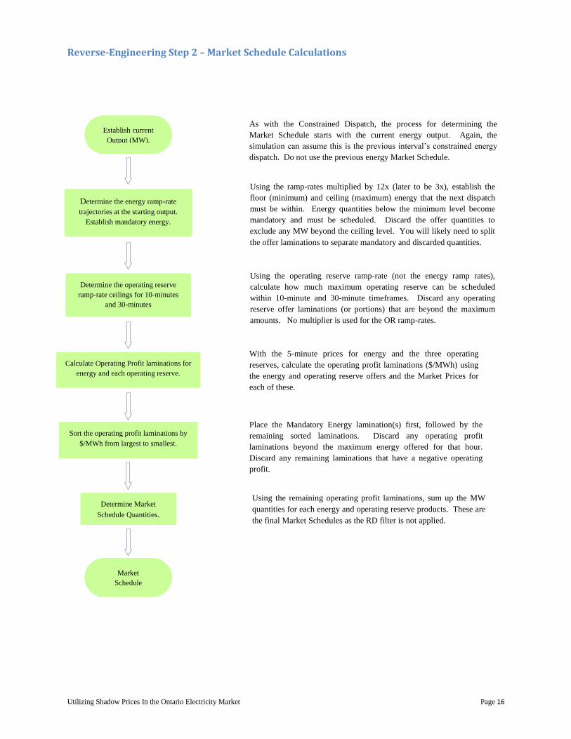
Reverse-Engineering Step 2 – Market Schedule Calculations

Using the ramp-rates multiplied by 12x (later to be 3x), establish the

floor (minimum) and ceiling (maximum) energy that the next dispatch

must be within. Energy quantities below the minimum level become

mandatory and must be scheduled. Discard the offer quantities to

exclude any MW beyond the ceiling level. You will likely need to split

the offer laminations to separate mandatory and discarded quantities.

As with the Constrained Dispatch, the process for determining the

Market Schedule starts with the current energy output. Again, the

simulation can assume this is the previous interval’s constrained energy

dispatch. Do not use the previous energy Market Schedule.

Determine the energy ramp-rate

trajectories at the starting output.

Establish mandatory energy.

Establish current

Output (MW).

Calculate Operating Profit laminations for

energy and each operating reserve.

With the 5-minute prices for energy and the three operating

reserves, calculate the operating profit laminations ($/MWh) using

the energy and operating reserve offers and the Market Prices for

each of these.

Sort the operating profit laminations by

$/MWh from largest to smallest.

Place the Mandatory Energy lamination(s) first, followed by the

remaining sorted laminations. Discard any operating profit

laminations beyond the maximum energy offered for that hour.

Discard any remaining laminations that have a negative operating

profit.

Determine Market

Schedule Quantities.

Using the remaining operating profit laminations, sum up the MW

quantities for each energy and operating reserve products. These are

the final Market Schedules as the RD filter is not applied.

Market

Schedule

Determine the operating reserve

ramp-rate ceilings for 10-minutes

and 30-minutes

Using the operating reserve ramp-rate (not the energy ramp rates),

calculate how much maximum operating reserve can be scheduled

within 10-minute and 30-minute timeframes. Discard any operating

reserve offer laminations (or portions) that are beyond the maximum

amounts. No multiplier is used for the OR ramp-rates.


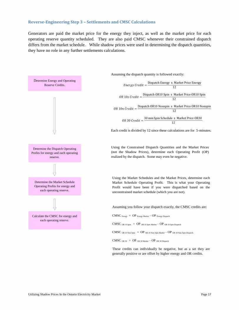
Reverse-Engineering Step 3 – Settlements and CMSC Calculations

Generators are paid the market price for the energy they inject, as well as the market price for each

operating reserve quantity scheduled. They are also paid CMSC whenever their constrained dispatch

differs from the market schedule. While shadow prices were used in determining the dispatch quantities,

they have no role in any further settlements calculations.

Assuming the dispatch quantity is followed exactly:

Each credit is divided by 12 since these calculations are for 5-minutes.

Determine Energy and Operating

Reserve Credits.

Determine the Dispatch Operating

Profits for energy and each operating

reserve.

Using the Constrained Dispatch Quantities and the Market Prices

(not the Shadow Prices), determine each Operating Profit (OP)

realized by the dispatch. Some may even be negative.

Determine the Market Schedule

Operating Profits for energy and

each operating reserve.

Using the Market Schedules and the Market Prices, determine each

Market Schedule Operating Profit. This is what your Operating

Profit would have been if you were dispatched based on the

unconstrained market schedule (which you are not).

Calculate the CMSC for energy and

each operating reserve.

Assuming you follow your dispatch exactly, the CMSC credits are:

CMSC Energy = OP Energy Market – OP Energy Dispatch

CMSC OR 10 Spin = OP OR 10 Spin Market – OP OR 10 Spin Dispatch

CMSC OR 10 Non-Spin = OP OR 10 Non-Spin Market – OP OR 10 Non-Spin Dispatch

CMSC OR 30 = OP OR 30 Market – OP OR 30 Dispatch

These credits can individually be negative, but as a set they are

generally positive or are offset by higher energy and OR credits.


Sygration Generation Market Simulator

The Sygration Generation Market Simulator is a subscription-based service based on the design described

above. It validates the submitted energy and operating reserve offers just as the IESO system does, then

processes every 5-minutes of historical data to generate dispatch and settlements reports. The service

allows market participants to test various bid strategies or fine-tune their offers using the historical

analysis. The user selects the delivery point and timeframe of interest, and submits offers for energy and

each of the three classes of operating reserve just as they would for the IESO.

The simulator has implemented the algorithm described earlier6, along with some additional rules for

marginal bids and indifferent market choices (when incremental operating profit is the same for energy

and operating reserve). The service accesses a large database of historical shadow and market prices and

6 The Reserve Loading Point is not implemented exactly as in the DSO. Instead, it is applied as the minimum generation level

that must be scheduled in the prior interval before operating reserve can be scheduled in the next interval. Low and high

operating limits, used in the RD filter, have also not been implemented.


calculates the dispatch quantities, market schedules, settlements credits and CMSC as if the offers had

been used for real.

Calculations are always based on the 5-minute historical pricing data. However, the output can be

summarized to show the hourly average and totals (as shown above) or daily average and totals. In

addition, a Monthly Summary and Hourly Profile report is generated.

Timestamps

(Hourly summary selected)

Market Prices

Energy & OR

Constrained

Dispatch (MW)

Settlement Credits

including CMSC


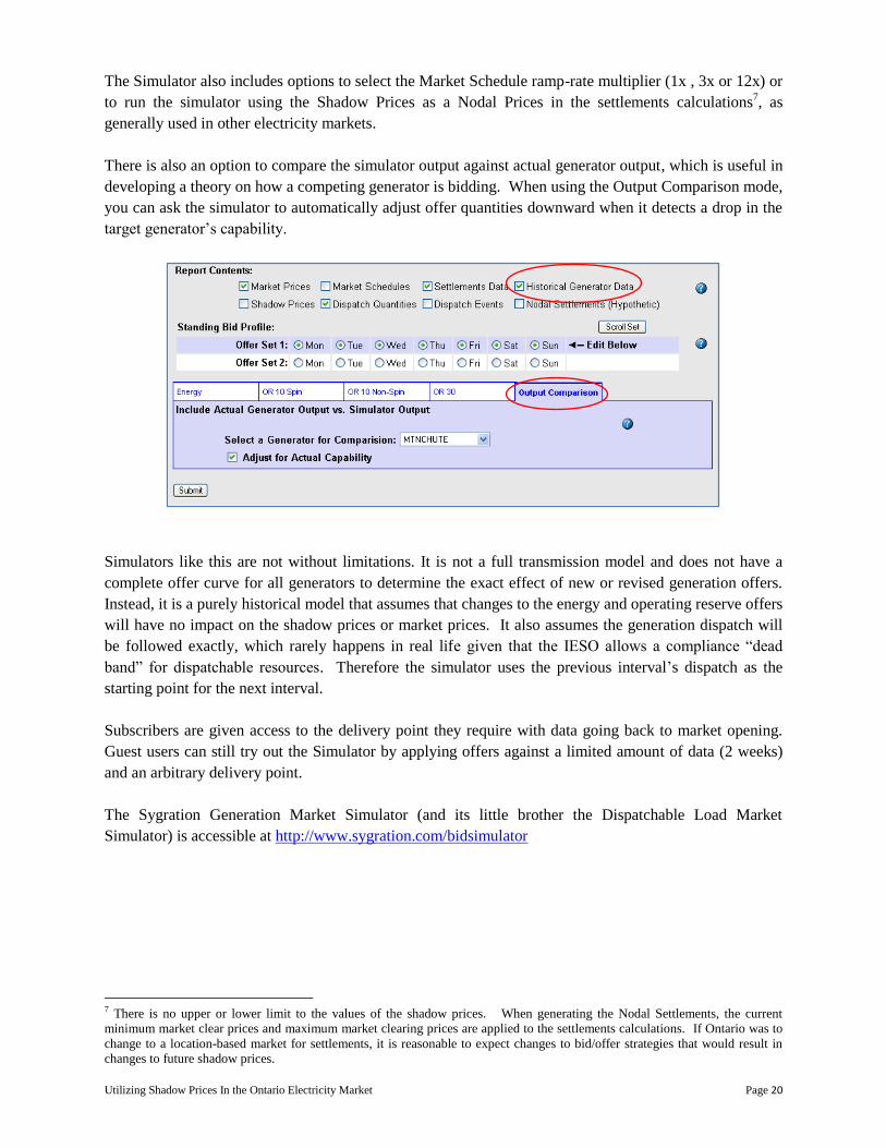
The Simulator also includes options to select the Market Schedule ramp-rate multiplier (1x , 3x or 12x) or

to run the simulator using the Shadow Prices as a Nodal Prices in the settlements calculations7, as

generally used in other electricity markets.

There is also an option to compare the simulator output against actual generator output, which is useful in

developing a theory on how a competing generator is bidding. When using the Output Comparison mode,

you can ask the simulator to automatically adjust offer quantities downward when it detects a drop in the

target generator’s capability.

Simulators like this are not without limitations. It is not a full transmission model and does not have a

complete offer curve for all generators to determine the exact effect of new or revised generation offers.

Instead, it is a purely historical model that assumes that changes to the energy and operating reserve offers

will have no impact on the shadow prices or market prices. It also assumes the generation dispatch will

be followed exactly, which rarely happens in real life given that the IESO allows a compliance “dead

band” for dispatchable resources. Therefore the simulator uses the previous interval’s dispatch as the

starting point for the next interval.

Subscribers are given access to the delivery point they require with data going back to market opening.

Guest users can still try out the Simulator by applying offers against a limited amount of data (2 weeks)

and an arbitrary delivery point.

The Sygration Generation Market Simulator (and its little brother the Dispatchable Load Market

Simulator) is accessible at http://www.sygration.com/bidsimulator

7 There is no upper or lower limit to the values of the shadow prices. When generating the Nodal Settlements, the current

minimum market clear prices and maximum market clearing prices are applied to the settlements calculations. If Ontario was to

change to a location-based market for settlements, it is reasonable to expect changes to bid/offer strategies that would result in

changes to future shadow prices.

http://www.sygration.com/bidsimulator


Author

Tom Hilbig, B.E.Sc., P.Eng

Sygration

905-593-1416

www.sygration.com

References

Introduction to Ontario’s Physical Markets, IESO

http://www.ieso.ca/imoweb/pubs/training/IntroOntarioPhysicalMarkets.pdf

Congested Management Settlement Credits – Recorded Presentation, IESO

http://www.ieso.ca/imoweb/marketplaceTraining/cmsc_presentation.asp

Day Ahead Market Project – How the DSO Calculates Nodal Prices, IESO

http://www.ieso.com/imoweb/pubs/consult/mep/DAM_WG_2003Oct20_DSONodal.ppt

Market Operating System. Validation Rules/Messages and Abbreviations, IESO

http://www.ieso.ca/imoweb/pubs/ti/MP_Submissions/ValidationRulesMsgAndAbbrev.rtf

Market Manual 4: Market Operations, Part 4.3 Real-Time Scheduling of the Physical Markets, IESO

http://www.ieso.ca/imoweb/pubs/marketOps/mo_RealTimeScheduling.pdf

Ontario Market Rules Chapter 7 System Operations and Physical Markets, IESO

http://www.ieso.ca/imoweb/pubs/marketRules/mr_chapter7.pdf

Ontario Market Rules Appendix 7.5 The Market Clearing and Pricing Process, IESO

http://www.ieso.ca/imoweb/pubs/marketRules/mr_chapter7appx.pdf

Ontario Market Rules Chapter 9, Settlements and Billing, IESO


Quick Take 20 - Joint Optimization of Energy and Operating Reserve, IESO

http://www.ieso.ca/imoweb/pubs/training/QT20_JointOptimization.pdf

Real-time Energy Market Dispatch Shadow Prices Report Specification, IESO

http://www.ieso.ca/imoweb/pubs/ti/Market_Results/MR_DispRTEMConstShdwPrcRpt.pdf

Sygration Generation Market Simulator Design Reference, Sygration

http://www.sygration.com/bidsimulator/gsdesign.html

Board Denies Review of Ramp Rate Amendment, Stikeman Elliott

http://www.stikeman.com/cps/rde/xchg/se-en/hs.xsl/9005.htm#9012

Copyright © 2007 Sygration

http://www.ieso.ca/imoweb/pubs/training/IntroOntarioPhysicalMarkets.pdf

http://www.ieso.ca/imoweb/marketplaceTraining/cmsc_presentation.asp

http://www.ieso.com/imoweb/pubs/consult/mep/DAM_WG_2003Oct20_DSONodal.ppt

http://www.ieso.ca/imoweb/pubs/ti/MP_Submissions/ValidationRulesMsgAndAbbrev.rtf

http://www.ieso.ca/imoweb/pubs/marketOps/mo_RealTimeScheduling.pdf


http://www.ieso.ca/imoweb/pubs/marketRules/mr_chapter7appx.pdf


http://www.ieso.ca/imoweb/pubs/training/QT20_JointOptimization.pdf

http://www.ieso.ca/imoweb/pubs/ti/Market_Results/MR_DispRTEMConstShdwPrcRpt.pdf

http://www.sygration.com/bidsimulator/gsdesign.html

http://www.stikeman.com/cps/rde/xchg/se-en/hs.xsl/9005.htm#9012

utilizing shadow prices in the ontario electricity market · pdf fileutilizing shadow prices...

Documents