Dedicated to my parents

List of papers

This thesis consists of the following papers, which will be referred to in the text by their Roman numerals:

I Linde, N., and L. B. Pedersen (2004), Characterization of a fractured granite using radio magnetotelluric (RMT) data, Geophysics, 69, 1155-1165.

II Linde, N., and L. B. Pedersen (2004), Evidence of electrical anisotropy in limestone formations using the RMT technique, Geophysics, 69,909-916.

III Linde, N., S. Finsterle, and S. Hubbard, Inversion of tracer test data us-ing tomographic constraints, Submitted to Water Resources Reseach, in revision.

IV Linde, N., J. Chen, M. B. Kowalsky, and S. Hubbard, Hydrogeophysi-cal parameter estimation approaches for field scale characterization, tobe published in Applied Hydrogeophysics, edited by H. Veerecken et al., Springer.

V Linde, N., A. Binley, A. Tryggvason, and L. B. Pedersen, Joint inver-sion of electrical resistance and GPR traveltime data applied to unsatu-rated sandstone, Manuscript.

The Society of Exploration Geophysics (papers I and II) kindly gave per-mission to reprint the papers. Additional papers written during my PhD stud-ies but not included in this thesis:

Beylich, A. A., E. Kolstrup, N. Linde, L. B. Pedersen, T. Thyrsted, D. Gintz, and L. Dynesius (2003), Assessment of chemical denudation rates using hydrological measurements, water chemistry analysis and electromagnetic geophysical data, Permafrost and Periglacial Proc-esses, 14, 387-397.

Beylich, A. A., E. Kolstrup, T. Thyrsted, N. Linde, L. B. Pedersen, and L. Dynesius (2004), Chemical denudation in arctic-alpine Latnjavagge

(Swedish Lapland) in relation to regolith as assessed by radio magneto-telluric-geophysical profiles, Geomorphology, 57, 303-319.

Contents

1 Introduction .........................................................................................11

2 Petrophysical basis...............................................................................132.1 Hydrogeological properties ........................................................132.2 Electrical properties....................................................................152.3 Petrophysical relationships between electrical and hydrogeological properties .......................................................................17

2.3.1 Electrical conductivity ...........................................................172.3.2 Permittivity ............................................................................18

3 A brief review of selected electromagnetic methods...........................203.1 Radio magnetotellurics...............................................................203.2 Ground penetrating radar............................................................223.3 Electrical resistance tomography................................................24

4 A few remarks on inverse theory.........................................................264.1 What is an inverse problem? ......................................................264.2 Objective functions.....................................................................27

5 Summary of papers ..............................................................................305.1 Paper I.........................................................................................30

5.1.1 Summary................................................................................305.1.2 Conclusions............................................................................33

5.2 Paper II .......................................................................................345.2.1 Summary................................................................................345.2.2 Conclusions............................................................................38

5.3 Paper III ......................................................................................385.3.1 Summary................................................................................385.3.2 Conclusions............................................................................41

5.4 Paper IV......................................................................................415.4.1 Summary................................................................................425.4.2 Conclusions............................................................................43

5.5 Paper V.......................................................................................435.5.1 Summary................................................................................435.5.2 Conclusions............................................................................46

6 Discussion and conclusions .................................................................48

6.1 Radio magnetotellurics in hydrogeophysics...............................486.2 Tracer test data in hydrogeophysics ...........................................496.3 Parameter estimation in hydrogeophysics ..................................496.4 Joint inversion and regularization ..............................................50

7 The future of hydrogeophysics ............................................................51

8 Summary in Swedish ...........................................................................55

9 Acknowledgements..............................................................................57

10 References ...........................................................................................59

Abbreviations

1D One-dimensional 2D Two-dimensional 3D Three-dimensional CSAMT Controlled Source Audio Magneto-

telluricsCRIM Complex Refractive Index Model EM Electromagnetic ERT Electrical Resistance Tomography GPR Ground Penetrating Radar MOG Multiple-Offset Gather MT Magnetotellurics RMT Radio Magnetotellurics ZOP Zero-Offset Profile

11

1 Introduction

Our society’s obsession with economical development and its preference for technological solutions will without any doubt continue to create environ-mental problems of increasing complexity. My PhD work focused on the hydrogeological characterization effort that often is a prerequisite for the understanding and solution of environmental problems. In particular, the focus was on the use of electromagnetic (EM) geophysical methods and their strengths and limitations in characterization of hydrogeological media.

Parameterization of spatially variable rock properties is needed in many environmental and engineering applications. Hydrogeological studies often suffer from too few hydrogeological measurements in relation to the vari-ability of hydraulic conductivity (e.g., McLaughlin and Townley, 1996); it is not uncommon that 106 hydraulic conductivity values are used in 3D simula-tions of contaminant transport.

Hydrogeophysics is an emerging research field with practitioners from both hydrogeology and geophysics where its practitioners try to improve our understanding of hydrogeological systems by the use of geophysical tech-niques (e.g., Hubbard and Rubin, 2005). The interface with neighboring research fields that have been termed near-surface geophysics, applied geo-physics, or environmental geophysics is rather fuzzy. I think that what most clearly distinguishes hydrogeophysics from neighboring research fields is that hydrogeophysicists generally focus on the hydrogeological processes and see geophysics as a potential tool to advance hydrogeology. Throughout this thesis, I refer to hydrogeophysics as all geophysical applications that provide qualitative or quantitative information about hydrogeological prop-erties or hydrogeological processes regardless of if the geophysical data are integrated with hydrogeological data and process knowledge.

Hydrogeophysics is best categorized in terms of spatial scale, method, and application.

In spatial scale, I distinguish between the drill core and borehole scale, the crosshole scale, the surface based scale, the airborne scale, and the continen-tal scale. In this work, I have only considered the crosshole (5-10m in my applications) and surface based scale (100-1000m in my applications).

In terms of method, I focused on EM methods. By EM methods, I refer to direct current (DC) methods in the zero-frequency limit (e.g., Daily et al., 1992; Zhang et al., 1995) and ground penetrating radar (GPR) in the high frequency limit (e.g., Davis and Annan, 1989; Annan, 2005), in addition to

12

methods that are classically grouped as EM methods, such as the radio mag-netotelluric (RMT) technique (e.g., Turberg et al., 1994; Bastani, 2001). Other methods not treated in this work, such as seismics (e.g., Steeples, 2005; Pride, 2005), self-potential (e.g., Sill, 1983, Revil et al., 1999), in-duced polarization (e.g., Marshall and Madden, 1959; Slater and Lesmes, 2002), gravity (e.g., Rodell et al., 2004), and Nuclear Magnetic Resonance (e.g., Shushakov, 1996; Legchenko and Shushakov, 1998) have been shown to be useful hydrogeophysical tools in some circumstances.

In terms of application, I have mainly focused on the saturated zone and my primary focus was on estimating hydraulic conductivity, either qualita-tively by delineating fracture zones or fracture anisotropy, or quantitatively by inversion of geophysical and hydrogeological data. Other hydrogeophysi-cal applications that have received considerable attention are, for example, moisture content monitoring (e.g., Huisman, 2003), delineation of hydro-geological units where the hydrogeological properties are approximately constant, so called hydrofacies (e.g., McKenna and Poeter, 1995; Hyndman and Gorelick, 1996), and monitoring of contaminant transport (e.g., Brewster et al., 1995).

My dissertation is based on five papers. In paper I, we applied the tensor RMT technique to study fracture zones on an island with bedrock dominated by highly resistive granite. In paper II, we developed an inversion method and applied the tensor RMT technique to study the electrical anisotropy of a limestone formation. In paper III, we developed a sequential inversion method to determine the hydraulic conductivity field by inversion of tracer test data with regularization defined by crosshole GPR velocity tomograms. In paper IV, we reviewed the choices that must be made in any hydrogeo-physical parameter estimation effort and discussed the value and limitations of three different approaches to hydrogeophysical parameter estimation. In paper V, we defined a methodology to jointly invert crosshole electrical re-sistance tomography (ERT) and GPR traveltime data. In addition, we evalu-ated an alternative regularization operator defined by the model covariance matrix, which we inferred from EM conductivity logs.

13

2 Petrophysical basis

2.1 Hydrogeological properties The governing equation describing fully saturated, transient, and anisotropic groundwater flow is

,qthSh sK (1)

where K (m/s) is the hydraulic conductivity tensor

,

zzzyzx

yzyyyx

xzxyxx

KKKKKKKKK

K (2)

and Ss is specific water storage, h (m) is hydraulic head, q (m3/s) is sinks and sources, x (m), y (m), z (m) are spatial co-ordinates that form a right-handed system with z increasing with depth, and t (s) is time.

Permeability is the fundamental rock property that quantifies the capacity of a porous media to transmit a fluid, whereas hydraulic conductivity is also dependent on the properties of the pore fluid. The relationship between hy-draulic conductivity and permeability is for saturated, homogeneous, and isotropic materials

,sw gkK (3)

where w (kg/m3) is the density of the pore water, g (m/s2) is the gravitational constant, ks (m2) is the permeability, and (Ns/m2) is the fluid dynamic vis-cosity. Water is the only liquid treated in this work and w, g, and are as-sumed to be constant.

14

Hydraulic conductivity of saturated media varies over several orders of magnitude even in fairly homogeneous aquifers (see Table 1); whereas the variability in porosity is much lower (see Table 2).

Table 1. Representative values of hydraulic conductivity for various rock types (adopted from Domenico and Schwartz, 1997, Table 3.2).

Material Hydraulic conductivity (m/s)

SEDIMENTARY Gravel 3 10-4-3 10-2

Coarse sand 9 10-7-6 10-3

Medium sand 9 10-7-5 10-4

Fine sand 2 10-7-2 10-4

Silt, loess 1 10-9-2 10-5

Till 1 10-12-2 10-6

Clay 1 10-11-4.7 10-9

Unweathered marine clay 8 10-13-2 10-9

SEDIMENTARY ROCKS Karst and reef limestone 1 10-6-2 10-2

Limestone, dolomite 1 10-9-6 10-6

Sandstone 3 10-10-6 10-6

Siltstone 1 10-11-1.4 10-8

Shale 3 10-13-2 10-9

CRYSTALLINE ROCKS Permeable basalt 4 10-7-2 10-2

Fractured igneous and metamorphic rock 8 10-9-3 10-4

Weathered granite 3.3 10-6-5.2 10-5

Unfractured igneous and metamorphic rocks 3 10-14-2 10-10

15

Table 2. Range in values of porosity (adopted from Domenico and Schwartz, 1997, Table 2.1).

Material Porosity (%)

SEDIMENTARY Gravel, coarse 24-36 Gravel, fine 25-38 Sand, coarse 31-46 Sand, fine 26-53 Silt 34-61 Clay 34-60 SEDIMENTARY ROCKS Sandstone 5-30 Siltstone 21-41 Limestone, dolomite 0-40 Karst limestone 0-40 Shale 0-10 CRYSTALLINE ROCKS Fractured crystalline rocks 0-10 Dense crystalline rocks 0-5 Basalt 3-35 Weathered granite 42-45

Based on the variability in hydraulic conductivity (see Table 1), its key role in groundwater flow (see equation 1), and the costs and intrusiveness of direct measurements of hydraulic conductivity it is not surprising that hy-drogeologists look for new data sources to estimate hydraulic conductivity in hydrogeological models (e.g., McLaughlin and Townley, 1996).

2.2 Electrical properties The electrical properties of crustal rocks are typically dominated by the wa-ter content and not by the electrical properties of the mineral constituents (e.g., Keller, 1987). Ground water is an electrolyte where the electrical con-ductivity is dependent on the mobility and number of ions in the solution. The electrical properties of a rock can be described by introducing a com-plex electrical conductivity ( *), a complex resistivity ( *), or a complex permittivity ( *) and they are related as

*,*

1* i (4)

where is the angular frequency ( =2 f ) and i= 1 (e.g., Lesmes and Friedman, 2005). The underlying physical properties are electrical conduc-tivity, (S/m), and permittivity, (F/m). The complex quantities in equa-

16

tion 4 describe both the conductive and capacitive properties of a rock. Elec-trical properties of rocks are often treated as isotropic, but are tensor quanti-ties.

Relative permittivity, , defined as

,0

(5)

where 0 is the permittivity of vacuum, 8.89 10-12 F/m, is more commonly used in GPR studies than permittivity.

The electrical resistivity/conductivity is often only weakly dependent on frequency at low frequencies (e.g., Lesmes and Friedman, 2005) and is as-sumed to be frequency independent in ERT and RMT applications.

The relative permittivity may, in the presence of clays, change signifi-cantly in the frequency range of interest in GPR applications (50 MHz to 1 GHz) because of interfacial polarization. Laboratory measurements per-formed by West et al. (2003) showed that Ottowa sand had no frequency dispersion, whereas a sample with 5% clay content had a relative permittiv-ity of 30 at 100 MHz and a relative permittivity of less than 5 at 950 MHz.

Electrical conductivities of rocks are extremely variable and there is sig-nificant variability within the same rock type, as well as overlaps in the re-sistivity values between different rock types (see Figure 1).

0.01 100100.1 1 1000 10 000 100 000

100 0.010.110 1 0.001 0.0001 0.00001

Resistivity (ohm-m)

Conductivity (S/m)

ShieldUnweathered rocks

Weathered layer

Glacial sediments

Sedimentary rocks

Water, Aquifers

Massive sulfides

GraphiteIgneous and

metamorphic rocks

Clays Gravel and sand

TillsShales Sandstone Conglomerate

Salt water Fresh water Permafrost

Sea Ice

Lignite, Coal Dolomite, Limestone

Mafic Felsic)Mottled zone

Duricrust

(Metamorphic rocks)

(Igneous rocks:Saprolite{

Figure 1. Typical ranges of resistivities of earth materials (adopted from Palacky, 1987, Figure 2).

17

2.3 Petrophysical relationships between electrical and hydrogeological properties

2.3.1 Electrical conductivity Archie’s law (Archie, 1942) and its derivatives are the most commonly used relationships to tie electrical conductivity of porous media to porosity and water saturation. Archie’s law has also been applied to fractured crystalline rock (e.g., Pedersen et al., 1992). A generalized formulation of Archie’s law is

,surfacemn

wSa (6)

where is the overall conductivity of the rock, w is the conductivity of the pore water, S is the water saturation, is the porosity, surface is the surface conductivity, and a, n, and m are fitting parameters. Table 3 shows typical values of a and m for different rock types.

Table 3. Forms of Archie’s law which can be used when lithology of a rock is known (after Keller, 1987, Table 10; Pedersen et al., 1992).

Description of rock a m

Weakly-cemented detrital rocks, such as sand, sandstone, and some limestones, with a porosity range from 25 to 45%. 0.88 1.37 Moderately well cemented sedimentary rocks, including sandstones and lime-stones, with a porosity range from 18 to 35%. 0.62 1.72 Well-cemented sedimentary rocks with a porosity range from 5 to 25%. 0.62 1.95 Rocks with less than 4% porosity, including dense igneous rocks and metamor-phosed sedimentary rocks.

1.4 1.58

Granite from the Gravberg-1 borehole, Siljan impact structure, Sweden. 2.0 1.45

Archie’s law can be useful in estimating porosity and the electrical con-ductivity of the pore water, but what about hydraulic conductivity? No gen-eral petrophysical relationship between electrical conductivity and hydraulic conductivity exists, which is not either too simplified to be useful or doesn’t assume unrealistic details in the available information about the rocks (e.g., Lesmes and Friedman, 2005).

Empirical relationships between electrical and hydraulic conductivity fall into two groups: one for clay-free media where it is often found that electri-cal and hydraulic conductivity are positively correlated because they both increase with increasing porosity; and one for clay-rich media where electri-cal and hydraulic conductivity often are negatively correlated. Purvance and Andricevic (2000) quoted results from field studies showing positive rela-tionships between the logarithm of electrical conductivity and the logarithm of hydraulic conductivity with correlation coefficients between 0.45 and 0.9,

18

and negative relationships between the logarithm of electrical conductivity and the logarithm of hydraulic conductivity with correlation coefficients between -0.27 and -0.88 at sites with fine sediments and low electrical con-ductivity of the pore water. However, evidence of correlations at specific sites tells us little about the predictive power of using electrical conductivity to estimate hydraulic conductivity at other sites.

The only feasible approach is to estimate site-specific relationships using borehole logs or to estimate the relationship as a part of the inversion. These are topics that are discussed in papers III and IV; otherwise, geological un-derstanding might help us to estimate zones of higher hydraulic conductivity (paper I) or possible directions of electrical anisotropy (paper II).

Better estimations of hydraulic conductivity can be obtained if induced polarization measurements are included, because the specific surface area (i.e., the ratio of surface area to pore volume) can be estimated (e.g., Slater and Lesmes, 2002).

2.3.2 PermittivityDielectrical properties are often interpreted using the complex refractive index model (CRIM) (e.g., Alharthi and Lange, 1987; Roth et al., 1990) or the Topp’s (Topp et al., 1988) formula.

The CRIM for unsaturated media is

,1 saweff (7)

where eff is the relative permittivity of the rock, is water content, w is the relative permittivity of water ( w 80), a is the relative permittivity of air ( a=1), and s is the relative permittivity of the rock matrix ( s=4-8, but sig-nificantly higher in clay mixtures). The CRIM is based on the assumption that the EM waves travel through the different rock constituents in series. It is possible to correct for the decrease in w with increasing temperature and salinity (e.g., Lesmes and Friedman, 2005).

The Topp’s formula is a widely used empirical formula defined as

.7.761463.903.3 32eff (8)

More advanced relationships exist but the CRIM and Topp’s formula work well in most applications and it is often other error sources that deter-mine the accuracy of the estimated water content (see section 3.2).

There are no reliable relationships between hydraulic conductivity and relative permittivity and site-specific relationships must be established (e.g., Hubbard et al., 2001). However, time-lapse GPR data can be used to esti-

19

mate hydraulic conductivity (e.g., Kowalsky et al., 2004a; Kowalsky et al., 2004b). Time-lapse measurements have not been used in my work, and its potential is not further discussed.

20

3 A brief review of selected electromagnetic methods

3.1 Radio magnetotellurics Tensor RMT data was used in both papers and II of this thesis. Radio mag-netotellurics is not one of the common geophysical methods. A search using ISI Web of Science (http://www.isiknowledge.com/) revealed twelve articles where RMT data have been used (Turberg et al., 1994; Tezkan et al., 1996; Beamish et al., 2000; Tezkan et al., 2000; Persson and Pedersen, 2002; Bey-lich et al., 2003; Newman et al., 2003; Beylich et al., 2004; Linde and Peder-sen, 2004a; Linde and Pedersen, 2004b; Tezkan et al., 2005; Pedersen et al., 2005). I believe there are two major reasons why RMT are not used that much: first, multi-electrode resistivity equipment (e.g., Dahlin, 1993) has revolutionized the resistivity method making it possible to do much faster and more detailed resistivity imaging (e.g., Loke and Barker, 1996) com-pared with what was possible a decade ago, the second reason is that there are no satisfying commercial tensor RMT systems.

The tensor RMT method makes use of the electric and magnetic fields generated by induction of currents in the ground caused by distant radio transmitters (10-250 kHz). The EM waves can be treated as plane because the scale length of the external field is large compared with the penetration depth. Plane-wave conditions prevail in a homogeneous half-space when the source-receiver separation is greater than about four skin depths (see equa-tion 12) (Goldstein and Strangway, 1975; Zonge and Hughes, 1991), whereas a separation of up to 20 skin depths is necessary for conductive sediments over resistive basement (Wannamaker, 1997). The radio transmit-ters are typically hundreds to thousands of skin depths away.

Under plane-wave conditions there exists a unique linear transfer function (i.e., the impedance tensor Z) between the horizontal electric, Eh, and hori-zontal magnetic, Hh, fields for a given angular frequency, , (Cantwell, 1960)

21

,y

x

yyyx

yxxx

y

x

HH

ZZZZ

EE

(9)

where the subscripts x and y denote north and east, respectively. The appar-ent resistivity, app

jk , and phase, jk, of an impedance element, Zjk (where jk is xy or yx; the first subscript indicates the measurement direction of the elec-tric field and the second subscript indicates the measurement direction of the magnetic field), can be determined with the well-known formulae

,Z1 2

jk0

appjk (10)

where 0 is the permeability of vacuum (4 ·10-7 Vs/Am), and

,tan 1rjk

ijk

jk ZZ

(11)

where superscripts i and r denote the imaginary and real part of the imped-ance element, respectively. The phases provide information about the rela-tive changes in conductivity. For a 1D earth, phases below 45 indicate a resistor at depth and phases above 45 indicate a conductor at depth (e.g., Vozoff, 1991). The skin depth, , which is the depth at which the amplitude decayed to 37% of the amplitude at the surface, increases with resistivity and decreases with frequency according to

.500f

ppjk (12)

For example, the skin depth is 500m if the resistivity is 16 000 ohm-m, and the frequency used is 16 kHz.

The measured apparent resistivities are often affected by static shifts. Static shifts are caused by small-scale inhomogeneities near the surface (i.e., with dimensions much less than the skin depth at the highest recorded fre-quency). These inhomogeneities cause surface charges that lead to a shift in the apparent resistivity curve such that the shifted curve is parallel to the undistorted curve on a log apparent resistivity versus log frequency plot (e.g., Zhang et al., 1987; Bahr, 1988; Groom and Bailey, 1989). The electri-cal distortion is typically parameterized as

,0PZZ (13)

22

where Z0 is the undistorted impedance tensor and P is a 2x2 real tensor de-fined as

.2221

1211

PPPP

P (14)

The static shifts by definition do not affect the measured phases. The geomagnetic transfer function (i.e., the tipper vector T), defined in

equation 15, gives qualitative indications of lateral changes in the resistivity structure of the earth. One-dimensional conditions are indicated if the tipper values are close to zero. The tipper is defined as

,T

HH

HH

BAHy

x

y

xz T (15)

where superscript T denotes transposition. The real and imaginary parts of the tipper form induction arrows. The real induction arrow points away from conductive anomalies (Parkinson, 1962).

The RMT data used in papers I and II were collected with the newly de-veloped tensor RMT system, EnviroMT (Bastani, 2001). All electromagneticsignals between 10-250 kHz with a signal-to-noise ratio above 12 dB in the magnetic field are identified and stacked (typically 100 times). The electric and the magnetic noise levels are defined as the median filtered horizontal fields, where the width of the filter is defined by the user. The signal-to-noise ratio is then defined as the ratio between the horizontal power and the estimated noise (Pedersen et al., 1994). Transfer functions are estimated at nine frequencies (two for each octave) from 14-226 kHz following Bastani and Pedersen (2001). The standard deviations are estimated based on the signal-to-noise ratios of the signals from the identified transmitters.

3.2 Ground penetrating radar Multiple offset gather (MOG) ground penetrating radar (GPR) data were used in papers III, V, and in two of the case studies presented in paper IV. An introduction to GPR methods in hydrogeology is provided by Annan (2005).

There are two survey modes used in crosshole GPR. In the zero-offset profile (ZOP), the GPR antennae are kept in their respective wells at equal depths, and a single measurement is made at each depth as the antennae are simultaneously lowered, yielding a data set that can be collected quickly but that does not contain as much information as if collected for 2D tomographic

23

reconstruction. In the multiple-offset gather (MOG), the antennae are varied such that a large number of rays pass the volume between the boreholes at different angles. Tomography is needed to interpret MOG data.

In contrast to the diffusive nature of RMT signals, GPR signals are gov-erned by the wave equation, making it possible to use many of the process-ing techniques and inversion methods developed in seismics (e.g., Bregman et al., 1989). In most crosshole applications it is assumed that the GPR wave travels as an infinitely thin ray from the antennae to the receiver. The ray-approximation is not justified in crosshole applications if we try to image objects smaller than half of the wave length (e.g., Williamson, 1991; Wil-liamson and Worthington, 1993; Spetzler and Snieder, 2004). Surveys are also limited by the angular aperture, which in the top and bottom of the to-mogram might be a larger limitation than the ray-approximation (Rector and Washbourne, 1994). The travel time is

,R

dlruT (16)

where T is the travel time, u(r) is the slowness (i.e., inverse of velocity), at a coordinate in space r and dl is the incremental distance along the ray-path with total length R. In practice, equation 16 is calculated through discretiza-tion

,1

N

ikiik lut (17)

where tk is the travel time of the kth raypath, ui is the slowness estimate of the ith cell, lki is the length of the kth raypath in the ith cell, and N is the total number of cells.

A common assumption is that the wave travels along a straight ray-path, which is a reasonable assumption if the velocity contrasts are smaller than 10-20 % (Peterson et al., 1985), which is typical for semi- to unconsolidated sediments common in environmental applications.

The inverse problem can be solved in different ways. In paper III, the al-gebraic reconstruction technique (ART) (Peterson et al., 1985) was used and in paper V, a regularized least-squares problem using curvi-linear ray-paths (Podvin and Lecomte, 1991; Hole, 1992) was solved. The keys to obtaining successful inversion results are correct zero times (i.e., the time of signal initiation), which tend to drift (e.g., Peterson, 2001), accurate locations of transmitters and receivers (e.g., Dyer and Worthington, 1988; Peterson, 2001), and a large angular aperture (e.g., Rector and Washbourne, 1994). The quality of the resulting tomogram is mainly determined by the data and

24

survey design, not by the inversion method (J. Peterson, personal communi-cation, 2004).

The relation between relative permittivity, , and radar velocity, v, for low-loss material is (Davis and Annan, 1989)

,2

2

vc (18)

where c is the velocity of electromagnetic waves through air ( 3 108 m/s). Thus, it is possible to relate radar velocity to porosity (see equation 7) and water saturation (see Equation 8).

It is also possible to invert for electromagnetic wave attenuation, but this aspect of GPR is not discussed further (see e.g., Maurer and Musil, 2004). Attenuation limits the scale of GPR surveys to less than 10m in most appli-cations, but the scale can be much larger in crystalline rocks. Probably the most commonly used GPR frequency in hydrogeophysical studies is 100 MHz (e.g., Binley et al., 2001a; Hubbard et al., 2001).

3.3 Electrical resistance tomography In paper V, electrical resistance tomography (ERT) data was used in addition to MOG GPR data. Crosshole ERT uses most often four electrodes for each measurement; two current and two potential electrodes at different locations in two boreholes or at the surface in vicinity of the boreholes. The main ad-vantage of crosshole ERT compared with surface deployed ERT is that the resolution does not decrease with depth. One of the first hydrogeophysical applications of crosshole ERT was to study vadose zone (i.e., the unsaturated zone) dynamics (Daily et al., 1992). General aspects of dc resistivity are well covered in the literature (e.g., Ward and Hohmann, 1987; Binley and Kemna, 2005).

The 3D, isotropic electrical conductivity distribution, (r), the electrical potential, V(r), at a point r due to a single current electrode, idealized as a point source at the origin with strength I, are related by

,rIV (19)

with the Dirac delta function. The boundary conditions are

0nV (20)

25

at the ground surface, where n is the outward normal, and

0V (21)

at other, infinite boundaries (e.g., Binley and Kemna, 2005). The superposi-tion principle can be applied to calculate the resulting electrical potential field from any pair of current electrodes.

There must be galvanic contact between the electrodes and the surround-ings. Therefore it is necessary to backfill the boreholes to ensure good con-tact in vadose zone studies (e.g., Binley et al., 2001a). The best noise esti-mates in ERT surveys are obtained by comparing reciprocal data points, i.e., with current and potential electrodes interchanged (e.g., LaBrecque et al., 1996). Error sources not captured in such estimates are the misplacement of electrodes and coarse discretization, e.g., relative errors of 5% are possible if only two finite elements are placed between the electrodes (LaBrecque et al., 1996).

26

4 A few remarks on inverse theory

4.1 What is an inverse problem? Menke (1984), Tarantola (1987), and Parker (1994) reviewed general geo-physical inverse theory; McLaughlin and Townley (1996) provided an excel-lent review of hydrogeological applications.

The forward problem is to calculate the response of a system for a given model, initial-, and boundary conditions. Often, the forward problem is non-linear and involves partial differential equations. In 2D or 3D studies the forward problem is solved using finite differences or finite element methods. The forward problem is

,dmF (22)

where F is a N×M data kernel that is dependent of the model vector, m, of size M×1. The response of F(m) is a data vector, d, of size N×1.

The inverse problem is for a set of finite and noisy data, dobs, to infer one or several models, mest, which honors the data within the estimated data er-rors and any additional constraints. Geophysical inverse problems are often under-determined or mixed-determined making it necessary to regularize the problem (e.g., Menke, 1984). Regularization imposes constraints on the model, for example, by penalizing model roughness yielding models with a strong spatial correlation (Constable et al., 1987), or deviations from an a priori model (Marquardt, 1970). Alternative ways to achieve regularization are through model discretization (e.g., Smith et al., 1999), by estimating approximate inverses, e.g., by using truncated singular value decomposition (TSVD) (e.g., Golub and van Loan, 1996; Friedel, 2003) or by early termina-tion of iterative solution methods, such as LSQR (e.g., Paige and Saunders, 1982; Jacobsen et al., 2003).

27

4.2 Objective functions In this section, common objective functions and Occam’s inversion are in-troduced.

The data fit between the model response and the empirical data is often defined as

),-(- T2 mFdCmFd -1d)(d (23)

where 1dC is the inverse of the data covariance matrix. It is commonly as-

sumed that the entries in d are uncorrelated, rendering -1dC a diagonal matrix

that contains the inverses of the estimated variances of the observation er-rors; thus, more reliable data carry larger weight. The data covariance matrix can either be estimated or assumed to take certain values if the method does not allow an error estimate. There is an implicit assumption of Gaussian errors in this formulation of data fit.

A general description of the model norm assuming that the model pa-rameters can be regarded as random variables with a Gaussian distribution is

),-()-( T20

-1m0 mmCmmm (24)

where m0 is an a priori model of size M 1; and -1mC is the inverse of the

model covariance matrix, which characterizes the expected variability and spatial correlation of model parameters. However, the model covariance matrix is often unknown and it might be restrictive to damp the model to be close to an initial model, if no good initial model exists. Therefore, other model norms are typically defined using different measures of roughness (e.g., Constable et al., 1987), for example, the first derivatives of the model

),()( T mm1R (25)

where is an N N matrix given for 1D models by

.

110......

0110

(26)

A weighted least-squares objective function (equation 23) is used when no a priori information is available and when the inverse problem is well-posed without a regularization term. However, this is typically not the case and a priori information or regularization must be imposed, justified or not.

28

The corresponding objective function corresponds with the maximum a pos-teriori (MAP) estimate (e.g., Tarantola, 1987)

.)-()-()-( TT mFdCmFdmmCmm -1d0

-1m0 )( -MAPW (27)

This is a weighting of a priori assumptions and data. As mentioned above, we do not always have a good estimate of the model

covariance and the data errors. Furthermore, the inverse problem may still not have a unique solution if the spatial correlation length is short compared with the scale of the study. This is the reason why Occam’s inversion is so popular in geophysical applications. We briefly review Occam’s inversion (Constable et al., 1987), which was originally developed for magnetotelluric (MT) data, but has been applied to diverse problems, including ERT, e.g., the commercial software RES2DINV of Loke (1997). The goal of Occam’s inversion is to minimize R1 (see equation 25) (or any other measure of model roughness) subject to ,2

*2d where 2

* is the desired level of data misfit. Constable et al. (1987) solved this problem by minimizing the penalty func-tional W (m)

,-()-+)()(=)( T-1T mFdCmFmmm -1ddW (28)

where -1 acts as a trade-off parameter between the smooth well-conditioned problem defined by a heavy penalty of model roughness (i.e., is large) and the ill-conditioned problem defined by the data fit (i.e., is small). For each iteration, a line search is carried out for the that minimize 2

d if 2*

2d

or else for the maximum for which 2*

2d is satisfied.

Models based on Occam’s inversion fit the data to the level of the esti-mated data errors with the smoothest possible model. As mentioned above, Occam’s inversion was developed for interpretation of MT data, which is a technique that provides estimates of data errors and where we, due to the large depth of investigation, often have limited a priori information. Therefore, it is sensible to be as conservative as possible. However, Occam’s inversion provides only a single model that might have little useful relations to the earth that gave rise to the observed data (Ellis and Oldenburg, 1994). For example, it might be of little value to try to infer the spatial correlation structure of a physical property from models derived by Occam’s inversion. In short, Occam’s inversion of real data provides models that are smoother than the true structure. Ellis and Oldenburg (1994) argued that alternative approaches that emphasize the prior information and include the observed data, as a supplementary constraint, should be constructed. Please note that any a priori model or model covariance matrix could in principle be included in Occam’s inversion if the objective function to minimize is defined as (e.g., Siripunvaraporn and Egbert, 2000)

29

,)-()-()-()(W T-1T mFdCmFdmmCmmm -1d0

-1m0 )( - (29)

which is identical to the MAP estimate (see equation 27) if 2*

2d is

reached for =1. The objective function defined in equation 29 was used in papers I and II for the inversion of RMT data, as well as in the individual inversions of crosshole ERT and GPR data in paper V.

30

5 Summary of papers

5.1 Paper I Characterization of a fractured granite using radio magnetotelluric (RMT) data My first project as a PhD student was to evaluate a newly developed tensor RMT method, EnviroMT (Bastani, 2001), for characterization of fracture zones and electrical anisotropy. The site chosen for the first experiments was Ävrö, a small island (1.6 1.2 km2) in south-eastern Sweden. The highly resistive granite and the surrounding sea complicated the inversion and the interpretation of the inversion results.

5.1.1 Summary

Paper I focuses on the interpretation of a 950m long profile of RMT data using a station spacing of ten meters. The data were collected starting from the central part of Ävrö extending to approximately 20m from the eastern coast. The profile coincided with a seismic reflection profile (Juhlin and Palm, 1999) and a deep borehole in the central part of the profile where hy-draulic conductivity, electrical resistivity, and fracture density have been measured (Gentzschein et al., 1987).

The impedance tensors (see equation 9) and tipper vectors (see equation 15) were estimated following Bastani and Pedersen (2001). The apparent resistivities, phases, and the real induction arrows are shown in Figure 2. The apparent resistivities are above 10 000 ohm-m for several stations making displacement currents non-negligible (e.g., Persson and Pedersen, 2002).

One-dimensional inversions with and without displacement currents in-cluded confirmed that neglecting displacement currents give a false conduc-tor in the upper few meters and that the resistivity of the basement is se-verely over-estimated.

31

4.24.65.05.4

a)

Log1

0f (

Hz)

b)

4.24.65.05.4

c)

Log1

0f (

Hz)

d)

4.24.65.05.4

e)

Log1

0f (

Hz)

2..5 3 3..5 4 4..5

f)

0º 20º 40º 60º

y (m)

Log1

0f(

Hz)

Log10 (ohm-m)

5.24.94.64.3

200 400 600 800

00.250.5

g)ρ

200 400 600 800y (m)

0 200 400 600 8000y (m)

0

Figure 2. Estimated (a) apparent resistivities and (b) phases for the determinant data (Pedersen and Engels, 2005), followed by (c,d) the xy-data and (e,f) the yx-impedances. (g) The real induction arrows.

We calculated a rotationally invariant measure of phase differences (Bahr, 1991) and skew (Swift, 1967) in order to determine the dimensionality of the electrical conductivity structure along the profile. These analyses showed that the first 200m of the profile are 3D (this can also be seen on the induc-tion arrows in Figure 2g), the central part of the profile is essentially 1D, and the last part of the profile is approximately 2D.

Strike analysis following Zhang et al. (1987) did not reveal any consistent strike along the profile. We assumed a strike direction to the north (i.e., the x-direction) because it coincided with reflector C, the seashore, and was supported by the induction arrows (see Figure 2g). Thus, the Zxy data corre-spond to the TE-mode where current flow is parallel to the strike direction

32

and the Zyx data correspond to the TM-mode where current flow is perpen-dicular to the strike direction.

Unfortunately, there are no 2D inversion codes that include displacement currents and 3D inversions were computationally too intensive. The effects of the displacement currents decrease with frequency, which is seen by studying the condition under which displacement currents are negligible ( / <<1). Therefore, 2D inversions were performed for lower frequencies (14-56 kHz) only. We carried out 2D inverse modeling using Rebocc (Siri-punvaraporn and Egbert, 2000) and included the sea at the end of the profile as a priori information. The resulting models are shown in Figure 3. The 2D models contain a fracture zone in the beginning of the profile, increased conductivity below 300m, and a conductor dipping inland at the end of the profile.

400300200100

0a)

z (m

)

b)

0 200 400 600 800400300200100

0c)

y (m)

z (m

)

0 200 400 600 800

d)

y (m)

2 3 4 5Log10 (ohm-m)

C

C

C

C

D D

D D

ρ

Figure 3. Two-dimensional models based upon low-frequency data (14-56 kHz). (a) The TE mode, (b) the TM-mode, (c) the TE+TM mode, and (d) the determinant mode models are shown. Displacement currents were neglected. The labels C and D indicate seismic reflectors (Juhlin and Palm, 1999).

The 3D feature in the first 200m is related to seismic reflector C, see Fig-ure 3 (Juhlin and Palm, 1999), but is the conductor found at depth (see e.g., Figure 3c) a real conductor or only an effect of the surrounding sea? Fur-thermore, is the 2D feature at the end of the profile related to a fracture zone or is it only an artifact from the surrounding sea?

We performed 3D forward modeling with displacement currents included using the X3D code (Avdeev et al., 2002) to evaluate if the conductor dip-ping inland from the sea is a true conductor and to model the conductor in the beginning of the profile in 3D. The preferred 3D model, which ade-quately fitted the data at 20 and 56 kHz, is shown in Figure 4.

33

2250 m

1 800 m

10

8

4

36

105

5

4

5 10

3

5 m

The profile

3000ohm-m

1000ohm-m

500ohm-m

3000ohm-m1000

ohm-m

40 m

160 m

100 m

100 m

Other island

Mainland

Mainland

Ävrö

The sea

The sea

150 m

a) b)

3000 ohm-m

30 000 ohm-m

700 ohm-m

x

yy

z

3000 ohm-m

The sea0.8 ohm-mThe sea

30 000 ohm-m

700 ohm-m

1000 ohm-m

100ohm-m

3000ohm-m

Gra

dual

dec

reas

e in

resi

stiv

ities

The influence of this conductor is tested

The profile

The

fract

ure

zone

Figure 4. (a) Bird’s-eye view of the 3D model of Ävrö, its 3D fracture zone, and the surroundings (island, mainland, and sea). The depth of the sea is indicated at various places. A 10-m discretization was applied in the horizontal directions. (b) Cross-section in the y-z plane that follows the profile. The sea was modeled as a 5-m-thick layer with varying resistivities in order to model the correct conductance for the 3-10-m-deep sea.

5.1.2 ConclusionsA densely sampled profile of tensor RMT data was measured on an island where the bedrock is mainly composed of highly resistive granite. The elec-trical conductivity structure along the profile was studied using 1D and 2D inversions, as well as 3D forward modeling.

A comparison of 1D inversions, with and without displacement currents, illustrated that if displacement currents were not considered, a conductive layer that was too conductive at the top and a too resistive basement were modeled. These results demonstrated that a 2D inversion algorithm that in-clude displacement currents should be developed because it would facilitate and significantly improve the interpretation of RMT data measured over resistive formations.

The apparent resistivities and phases (14-56 kHz) was inverted assuming a strike direction to the north using Rebocc (Siripunvaraporn and Egbert, 2000), a 2D inversion code that does not include displacement currents. The resulting model based on the TE+TM data contains a weathered upper layer (20-40m depth) overlying a more intact granite. The granite is highly resis-tive—in many cases close to 100 000 ohm-m, indicating a very low concen-tration of wet fractures in the central part of the profile. The conductor in the beginning of the profile is probably associated with a seismic reflector (Juh-lin and Palm, 1999; see reflector C in Figure 3) and it is interpreted as a 150m wide saturated fracture zone.

34

Three-dimensional forward modeling supported the existence of a more conductive layer at about 300m depth of approximately 700 ohm-m. It is unlikely that pore fluid conductivities are higher than 1.5 S/m, which is the highest pore fluid conductivity found in the various boreholes drilled on the island (Gentzshein et al., 1987). We prefer an interpretation in terms of a massive fractured zone or a combination of several zones that are related to the fractured sections found in the borehole in the central part of the profile at 425-480m and 520-565m depth. A large number of shorter sub-horizontal reflectors observed on the coinciding reflection seismic section (see Figures 6 and 9 in Juhlin and Palm (1999)) in this depth interval support that inter-pretation.

5.2 Paper II Evidence of electrical anisotropy in limestone formations using the RMT techniqueThe second site chosen to evaluate EnviroMT was a limestone formation on the island of Gotland, Sweden. There were two objectives of this work: (1) to find a site where azimuthal electrical anisotropy was strong and unambi-guous; (2) to show that the tensor RMT method offers several advantages compared with the azimuthal resistivity method.

5.2.1 Summary Electrical anisotropy in a fractured rock formation may indicate that the rock formation is hydraulically anisotropic. Azimuthal resistivity surveys have, therefore, been applied in several groundwater studies (e.g., Taylor and Fleming, 1988; Ritzi and Andolsek, 1992; Lane et al., 1995) because azi-muthal resistivity surveys are non-invasive and relatively cheap compared with hydrological pump and tracer tests. Watson and Barker (1999) sug-gested that results presented in earlier work were unreliable because they used symmetric resistivity configurations and it is impossible to distinguish anisotropy from dipping layers or lateral changes in resistivity using sym-metrical configurations. Moreover, they illustrated that the offset Wenner technique could be used more reliably. However, all azimuthal resistivity configurations share inherent limitations, the most severe is that the configu-ration must be rotated in steps of 10 -20 making surveys slow, which in practice limits surveys to a few individual stations.

The tensor RMT method provides a fast and reliable method to study electrical anisotropy on a scale of 10 to 1000m. The tensor RMT measure-ments that are used to study electrical anisotropy are the same as in any ten-sor RMT survey and two persons can survey up to 100 stations a day. An analysis of electrical anisotropy is only carried out if the impedance tensor

35

(Equation 9) and tipper vector (Equation 15) indicate a 1D azimuthally ani-sotropic electrical conductivity structure.

We developed an inversion code to estimate, for each layer, the thickness of the layer (h (m)), the direction of anisotropy, and the electrical resistivity along the direction of anisotropy, as well as in the perpendicular direction. We based our forward code on the work by Yin (1999) and Yin and Maurer (2001). We solved the inverse problem by minimizing a least-squares objec-tive function to the estimated error levels in the data. Stability of the inver-sion was enforced using truncated singular value decomposition (Golub and van Loan, 1996) and Marquardt damping (Marquardt, 1963).

Tensor RMT profiles with a station spacing of ten meters were collected over a limestone formation at File-Hajdar on Gotland, Sweden. Figure 5 shows the apparent resistivities, phases, and the real part of the tippers for one of the collected profiles. A conductor is shown at the top, followed by a resistor and a conductor. Resistivity values, as well as the thickness of the resistive layer, increase in the northern part of the profile. The yx data (Fig-ure 5b and 5d) are clearly more resistive than the xy data (Figure 5a and 5c). Tippers (Figure 5e and 5f) do not reveal any major anomalies along the pro-file. A strike analysis following Zhang et al. (1987) showed together with the estimated transfer functions that the limestone formation is azimuthally ani-sotropic with a fairly consistent strike direction.

36

a) xy

f (kH

z)

b) yx

204080

160c) xy

f (kH

z)

30º

50º

60ºd) yx

0204080

160

x (m)

e) Ar

f (kH

z)

-0.1

0

0.1

0x (m)

200100 300 100 200 300

f) Br

40º

(ohm-m)

204080

160

400300200

app app NSNS

Figure 5. Apparent resistivity (a and b), phase (c and d), and real part of the tipper (e and f) for both xy and yx polarizations. The real part of the tipper, less than 0.15, indicates 1D conditions. Furthermore, the phase differences of the two polarizations are considerable and consistent, indicating azimuthal anisotropy.

The inverted model without static shifts is shown in Figure 6. We de-creased the effects of static shifts by taking the median of the impedance elements for the measured station and four neighboring stations. The lime-stone formation (layer 2) displays a distinct anisotropy (Figure 6a and 6b). The anisotropy factor in the limestone formation was estimated to be 3.7.

37

0 100 200 300

(oh

m-m

)

a)

0 100 200 300

(ohm

-m)

b)

0 100 200 300-180

-135

-90

-45

0

x (m)

Stri

ke (º

)

c) S trike dir. layer 2

0 100 200 30030

25

20

15

x (m)

z (m

)

d) Depth to layer 3

laye r 1laye r 2laye r 3

10

10

10

104

1

2

3

10

10

10

104

1

2

3

S N NS

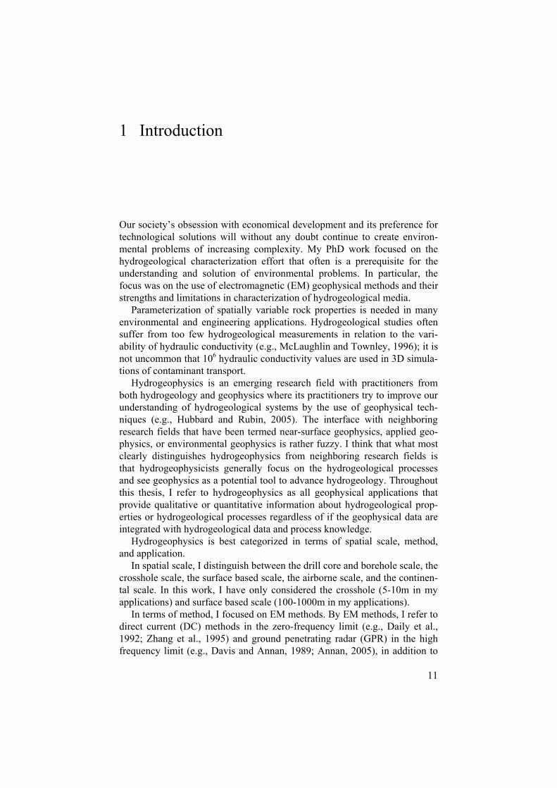
Figure 6. Three-layer azimuthal anisotropy model based on inversion of the median of five neighboring stations and without considering electrical distortion. Resistivity values in the strike direction (a) and the perpendicular direction (b) show that the second layer is anisotropic. The quantity, /h, not the resistivity, is presented for layer 1. The modeled strike directions in the second layer (c) do not change very much along the profile. The interface between the second and third layers (d) is modeled to increase from 17 m to 22 m.

The reliability of the presented model was assessed based on the results from 2D isotropic inversion of the determinant data (Pedersen and Engels, 2005) and from lithological logs in the vicinity of the profile.

The depths to the third layer coincided relatively well with the transition from a resistor to a conductor in the 2D isotropic model. Furthermore, the resistivities in the directions parallel and perpendicular to strike, for both layer 2 and 3, had values that are below and above the isotropic model, re-spectively. This was expected because the resistivity model based on deter-minant data corresponds to a mean resistivity.

The profile was in the vicinity of six lithological logs that show a rela-tively undisturbed limestone formation in the upper section. The lithological logs indicate a transition from the limestone formation to a shale formation with alternating layers; the clay content in the shale increases with depth. The interface between layer 2 and 3 (see Figure 6d) corresponds within 2m to the depth at which the clay content in the lithological logs increased to 25%. Models based on RMT data give a volume estimate, and cannot detect the thin clay layers embedded in the limestone formation. The data fit (RMS 1 for an error floor of 3%) gave further support to the validity of the results.

38

5.2.2 ConclusionsA 1D inversion code for tensor RMT data with an azimuthal electrical

anisotropy signature was developed and successfully applied to a densely sampled profile measured over limestone.

It is clear that the massive limestone at File-Hajdar is electrically anisot-ropic (see Figure 6). But why? Major fracture zones in the region have a strike at 340 to 350 north, and it is likely that fractures on a more local scale have the same dominant strike. The groundwater reservoir is generally full in early April when the fieldwork was performed. Therefore it can be assumed that all fractures in the limestone were water filled. The consistent strike in the second layer and the small changes in resistivity along the pro-file indicate that the aquifer system has an anisotropic hydraulic conductivity on a regional scale. However, pump tests would be necessary to confirm and quantify the hydraulic anisotropy.

The RMT technique is a good alternative to azimuthal resistivity surveys and the EM azimuthal resistivity method (Slater et al., 1998). A clear advan-tage of the presented method is that data are measured with a traditional survey and that no rotation of the electrode configuration is necessary. Fur-thermore, a number of transfer function estimates in the frequency range 10-250 kHz can easily be obtained and inverted.

5.3 Paper III Inversion of tracer test data using tomographic constraints Most of the work in hydrogeophysics has been carried out using crosshole methods. In crosshole methods, I saw an opportunity for quantitative estima-tion of hydraulic conductivity, something that cannot be achieved from the data available in papers I and II. The remaining papers (III, IV, and V) focus on crosshole data and how to use this information in hydrogeologically meaningful ways. Paper III describes a new methodology to estimate hy-draulic conductivity fields using radar tomograms and tracer test data. In addition, the results presented in paper III illustrate how different error sources influence the hydraulic conductivity estimates.

5.3.1 Summary Estimation of hydrogeological properties using geophysical data is often based on well-known petrophysical relationships between the geophysical and the hydrogeological property under interest (e.g., Binley et al., 2002; Alumbaugh et al., 2002) or by estimating an empirical relationship estab-lished from co-located geophysical and hydrogeological data, where the geophysical model is used to extrapolate the hydrogeological model to do-

39

mains insensitive to the hydrogeological data (e.g., Chen et al., 2001; Hub-bard et al., 2001). There is empirical evidence that geophysical data have improved estimates of hydrogeological properties compared with cases where only hydrogeological data were used (e.g., Hubbard et al., 2001; Scheibe and Chien, 2003). Unfortunately, the approaches to hydrogeophysi-cal parameter estimation mentioned above can be limited because petro-physical relationships may vary as a function of hydrogeological heterogene-ity (e.g., Prasad, 2003) and because the resolution of geophysical tomograms varies within the model and are dependent on survey design and data errors (e.g., Peterson, 2001; Day-Lewis and Lane, 2004), making it difficult to estimate the accuracy of the resulting models. An additional limitation is that petrophysical relationships in many applications are weak.

A number of studies have been performed where the geophysical data were used mainly to identify zones where geophysical and hydrogeological properties were assumed to be constant. The hydrogeological properties within these zones were estimated using tracer test data (e.g., Hyndman et al., 1994; McKenna and Poeter, 1995; Hyndman and Gorelick, 1996; Hynd-man et al., 2000). Paper III advances the use of tracer test and crosshole GPR travel time data to estimate hydraulic conductivity (crosshole seismics were used in the studies mentioned above), by assuming different petrophysical relationships in different zones of the tomogram, and by a detailed study of how different types of data acquisition errors affect the estimates.

In short, the methodology works as follows. First, an inversion of the MOG GPR travel time data is performed. Second, velocity zones within the tomogram are identified with a clustering algorithm. A zone is defined by a group of connected pixels where all pixels are either above or below the median velocity. Third, the misfit between observed and simulated tracer test data are minimized by estimating linear relationships between radar velocity and hydraulic conductivity for each zone (the non-stationary inversion) or by estimating one relationship for the whole study area (the stationary inver-sion).

The inversion methodology is based on two major assumptions: Major spatial variations in hydraulic conductivity are associated with spatial varia-tions in the radar tomogram; unknown, stationary, and linear petrophysical relationships are valid within specific zones of the tomogram.

The methodology was tested for 2D synthetic examples where a 9.3m line source using a slug injection of 280 g bromide was injected in one borehole and synthetically sampled with multilevel samplers every 0.9m in depth at another vertical borehole every 18 hours over 19 days. For each example, a hypothetical MOG GPR survey that consisted of 628 travel times was col-lected between the two boreholes and subsequently inverted using different acquisition errors (i.e., incorrect zero-times; random errors in the horizontal position of the sources and receivers; offset errors in the horizontal and ver-

40

tical separation between boreholes; and dipping boreholes that are assumed to be vertical).

The flow and transport simulations were calculated with TOUGH2 (Pruess et al., 1999), the GPR data were inverted using the algebraic recon-struction technique (Peterson et al., 1985), and the hydrogeophysical inver-sion was performed using a modified version of iTOUGH2 (Finsterle, 1999).

Figure 7 shows an example where one zone (approximately between 9 and 10m depth and 0-3m along the x-axis) has a different petrophysical rela-tionship between radar velocity and hydraulic conductivity compared to the other parts of the tomogram. The true radar velocity model (Figure 7a) was well resolved by the tomography (Figure 7b) because the hypothetical acqui-sition errors were very small for this example. The true hydraulic conductiv-ity field (Figure 7c) was accurately estimated by the non-stationary inversion (Figure 7d), whereas the stationary inversion (Figure 7e) images a false hy-draulically resistive zone, which is clearly indicated by the residuals of the true and the estimated fields (Figures 7f and 7g). Finally, scatter plots show that the correlation coefficient between the estimated and the true hydraulic conductivity model was higher for the non-stationary inversion (Figures 7h) compared with the stationary inversion (Figures 7i).

d) Non-stationary

e) Stationary

-5.0

-4.8

-4.6

-4.4

-4.2

-4.0

a) True velocity

58

60

62

64

Velo

city

(m/µ

s)

12

9

6

3

Dep

th (m

)

x (m)0 2 4

-0.5

0

0.5f) Nonstationary g) Stationary

Y(lg

(m/s

))^

Y-Y

(lg(m

/s))

^

−5 −4

−5

−4

12

9

6

3

Dep

th (m

)

b) Tomogram c) Y

h) Nonstationary i) Stationary

x (m)0 2 4

x (m)0 2 4

x (m)0 2 4

x (m)0 2 4

x (m)0 2 4

x (m)0 2 4

−5 −4Y (lg(m/s))

^

Y (lg(m/s))

Y(lg

(m/s

))

Figure 7. Results from the case where one zone has a different petrophysical rela-tionship compared with the others. (a) The true velocity model, (b) the tomogram, (c) the true hydraulic conductivity field, (d) hydraulic conductivity estimate from nonstationary inversion, (e) hydraulic conductivity estimate from stationary inver-sion, (f) residuals of true and estimated hydraulic conductivity field from stationary inversion, (h) scatter plot of true and estimated hydraulic conductivity field from nonstationary inversion, (i) scatter plot of true and estimated hydraulic conductivity field from stationary inversion.

41

5.3.2 ConclusionsAn inversion methodology aiming at estimating the hydraulic conductivity field by inverting tracer test data was developed and applied to synthetic 2D examples, where the regularization of the inverse problem was defined by radar velocity tomograms.

It was found that radar velocity tomograms improve models of hydraulic conductivity fields, compared with just using tracer data, if the correlation coefficient between radar velocity and hydraulic conductivity is above 0.5. Also, the non-stationary inversion performs better than the stationary inver-sion if the petrophysical relationship is spatially variable or if inversion arti-facts are present. Lastly, meticulous care in minimizing geophysical data errors is needed if the resulting tomograms are to be used for quantitative estimation of hydrogeological properties; inaccurate measurements of a few degrees about borehole deviations make the geophysical models essentially useless.

The methodology was recently generalized to 3D and applied to a site in Virginia (Linde et al., 2005), US, where the geology is composed of peat layers and clayey silts, in addition to sands and gravelly sands (e.g., Hubbard et al., 2001). The results were compared with estimates using flowmeter data and radar tomograms (Chen et al., 2001) and both hydraulic conductivity estimates yielded a positive relationship between radar velocity and the loga-rithm of hydraulic condctivity, even though the sensitivity to radar velocity was lower when tracer data was used, which might be attributed to the coarse grid discretization used in the flow modeling.

One of the limitations of this work was that we used a sequential inver-sion approach (i.e., first inverting MOG GPR travel time data and using the resulting models to constrain the inversion of tracer test data). The draw-backs of such an approach are discussed in paper IV and a possible frame-work for joint inversion is presented in paper V.

5.4 Paper IV Hydrogeophysical parameter estimation approaches for field scale characterization The hydrogeophysical terminology is largely based on terms introduced in hydrogeology, geostatistics, and geophysics. Terms are not always consis-tently used and sometimes several terms refer to the same thing. Being new to hydrogeophysics I found it difficult to compare the scientific content in different papers and to assess what aspects of the problem that were tackled and what aspects were ignored. Paper IV is an attempt to formalize the dif-ferent steps in hydrogeophysical parameter estimation and to discuss the

42

strengths and weaknesses of different approaches to hydrogeophysical pa-rameter estimation.

5.4.1 Summary The inter-disciplinarity of hydrogeophysics and the wide range of applica-tions make hydrogeophysics poor in offering black-box solutions to real problems.

In paper IV, we discussed how model parameterization influences the re-sulting model (e.g., Auken and Christensen, 2004). Three broad classes of model parameterizations were defined: zonation (e.g., Carrera and Neuman, 1986); geostatistical parameterization (e.g., Hoeksema and Kitanidis, 1984); and Tikkonov regularization (e.g., Constable et al., 1987). Petrophysical relationships were categorized as either physically or empirically based; intrinsic- or model-based; weak or strong. Additionally, solutions of inverse problems using classical optimization or Monte-Carlo methods as well as the most common objective functions were discussed.

Potentially, categorization of hydrogeophysical parameter estimation ap-proaches could be based on the characteristics defined above. Our choice was instead to base the categorization on what stage the geophysical and hydrogeological data are linked. Three broad categories were defined: (1) direct mapping; (2) integration methods; and (3) joint inversion methods. Five case studies were presented to highlight the differences between the approaches.

Direct mapping is defined as a transformation of a geophysical model into a hydrogeological model, where hydrogeological data are only used to de-velop a petrophysical relationship or to provide a qualitative understanding of the relationship between the geophysical and hydrogeological property under interest. Direct mapping was illustrated by water content estimation using crosshole GPR, an application where direct mapping works well be-cause the petrophysical link is strong (see equations 7 and 8).

Integration methods refer to cases where the geophysical inversion is per-formed independent of hydrogeological data, and vice versa. The task is to interpolate available data or inverse models given their uncertainties, petro-physical relationships, and a priori information. Integration methods were illustrated by geochemical characterization, where the site-specific mutual dependence of GPR attenuation and extractable Fe(II) and Fe(III) concentra-tion on lithofacies (developed using co-located GPR attenuation pixel values and soil sample measurements) was used (Chen et al., 2004).

Finally, joint inversion methods refer to cases where the geophysical or hydrogeological inversions also utilize hydrogeological or geophysical data, respectively. Joint inversion methods were illustrated with zonation of hy-draulic conductivity using seismic travel times and tracer test data (Hynd-man et al., 1994; Hyndman and Gorelick, 1996; Hyndman et al., 2000); with

43

vadose zone parameter estimation using time-lapse ZOP GPR travel time data (Kowalsky et al., 2004a); and fracture delineation using seismic travel times and flow meter data (Chen et al., 2003).

5.4.2 ConclusionsIn paper IV, the different steps in hydrogeophysical parameter estimation were reviewed and three different parameter estimation approaches were defined and exemplified by case studies. Approaches for hydrogeophysical parameter estimation are likely to develop in many directions and a unified estimation method is not in sight.

Careful survey design and surveying, together with a good conceptual un-derstanding of the problem, of the petrophysical relationships, and the domi-nant processes are probably the most important factors in successful hydro-geophysical parameter estimation. As hydrogeophysics evolves we must put more emphasis on minimizing, estimating, and parameterization of the errors in our measurements. We need to improve our understanding of the validity of petrophysical relationships and put more emphasis on methods that are more closely linked to groundwater flow and hydraulic conductivity, such as self-potential and induced polarization methods.

We believe that approaches that we termed joint inversion methods are well suited to improve error estimates, to increase our knowledge about the worth of different data types, and to design field campaigns that have the potential to provide the best characterization for a given budget. However, joint inversion methods are in their infancy and the solution to many prob-lems can be adequately addressed using direct mapping or integration meth-ods.

5.5 Paper V Joint inversion of electrical resistance and GPR traveltime data applied to unsaturated sandstone The objectives of paper V were to improve models obtained by inversion of crosshole ERT and GPR data: (1) by using EM conductivity logs to define stochastic regularization operators; and (2) by joint inversion of crosshole ERT and GPR data. Paper V considers geophysical data only, but I think that concepts from paper V could be applied to joint inversion of geophysical and hydrogeological data.

5.5.1 Summary The site chosen for this study is located near Eggborough, North York-

shire, UK, where crosshole ERT and MOG GPR data were available. The

44

Sherwood Sandstone is a fluvially derived deposit consisting mainly of me-dium- and fine grained sandstones with a small and variable amount of clay (0-5%), where the fine-grained sands are thin beds 0.1 to 0.3m thick, sepa-rated by much thicker (1-3m) medium-grained units (West et al., 2003).

An exponential covariance model describing the variance and spatial cor-relation structure of electrical conductivity was inferred from EM conductiv-ity logs. The integral scales in the vertical direction and horizontal directions were estimated to be 3.5m and 17.5m, respectively. Circulant embedding and fast Fourier transform of this geostatistical model (Dietrich and Newsam, 1997) was used to efficiently and with moderate memory require-ments calculate a stochastic regularization operator, ,-1/2

mC where Cm is the model covariance matrix. Such stochastic regularization operators constitute a combination of smoothness and damping operators (Maurer et al., 1998). We assumed an exponential covariance model of radar slowness with the same integral scales as in the ERT inversion. A variance of 10% of the mean slowness was used; the variance is not so important because it will scale with the trade-off parameter, , found in equation 29.

The 3D inversion method is based on a regularized least-squares algo-rithm closely related to Occam’s inversion (Constable et al., 1987), which we solve using LSQR (Paige and Saunders, 1982). The tomograms obtained by using smoothness constraints (Figures 8b and 8d) are in good agreement with earlier models based on 2D inversions using the same data set (Binley et al., 2001b). The tomograms based on the stochastic regularization (Figures 8a and 8c) are more layered and therefore geologically more reasonable. All models reached a weighted RMS target misfit of 1, where the errors in the traveltimes were assumed to be 2 ns and a constant error of 0.0001 ohm and a relative error of 5% were assumed for the electrical resistances.

45

0 1 2 3 4 5 615

14

13

12

11

10

9

8

7

6

5

4

3

0 1 2 3 4 5 6

0.09

0.1

0.11

0.12

0.08

Velo

city

(m/n

s)

Distance from R3 (m)Distance from R3 (m)

Dep

th (m

)

c) d)

58

119

244

501

28

Res

istiv

ity (o

hm-m

)

Dep

th (m

)

Distance from R3 (m)

0 1 2 3 4 5 615

14

13

12

11

10

9

8

7

6

5

4

3

Distance from R3 (m)

0 1 2 3 4 5 6

a) b)

Figure 8. Individual inversions: (a) ERT with stochastic regularization; (b) ERT inversion with smoothness regularization; (c) MOG GPR inversion with stochastic regularizations; and (d) MOG GPR inversion with smoothness regularization.

46

Crosshole ERT models have the best resolution close to the boreholes (e.g., Binley and Kemna, 2005); whereas models based on MOG GPR traveltimes have the highest resolution in the central area of the tomogram (e.g., Day-Lewis and Lane, 2004). Joint inversion of crosshole ERT and GPR data can, therefore, improve the resolution of both models.

Petrophysical relationships between geophysical properties are in many cases weak and unknown. Therefore performing joint inversion through a petrophysical relationship is often a too strong assumption, which might bias the resulting models. A structural approach to joint inversion is a more con-servative choice (Haber and Oldenburg, 1997). Gallardo and Meju (2003) defined the cross-gradient function, which quantifies structural similarity. By minimizing the cross-gradient function together with more classical terms, such as data misfit and model roughness, it is possible to estimate two geo-physical models where the gradients of the models have the same or opposite directions, but where the actual petrophysical relationship between the two model properties can be unknown, non-stationary, and non-linear. Addition-ally, inversion with the cross-gradient function allows petrophysical relation-ships to be evaluated a posteriori. The cross-gradient function has been used to jointly invert surface based data (seismic refraction, ERT, and controlled source audio magnetotelluric (CSAMT) data) (Gallardo and Meju, 2003; Gallardo and Meju, 2004; Gallardo and Meju, 2005; Gallardo and Meju, submitted).

We defined a joint 3D inverse problem where we in addition to data mis-fit and regularization operators also penalize deviations from structural simi-larity quantified by the cross-gradient function. We gave equal weights to the electrical resistance and the GPR travel time data by first performing separate inversions and setting a constant standard deviation of the data types for which solutions with a weighted RMS of 1 can be found.

Joint inversion results of the crosshole ERT and GPR data are presently not available. The inversion is slow due to ill-conditioning, but the conver-gence is good after three iterations. We estimate that approximately six itera-tions will be needed to estimate models with a weighted RMS of 1.

5.5.2 ConclusionsCrosshole ERT and GPR data collected in unsaturated sandstone close to Eggborough, UK, were inverted individually with a new stochastic regulari-zation operator, as well as with traditional smoothness constraints, and jointly by minimizing the cross-gradient function (Gallardo and Meju, 2003) in addition to data misfit and smoothness constraints.

The stochastic operator was tested on both crosshole ERT (see Figure 8a) and MOG GPR data (see Figure 8c) where the geostatistical model was in-

47

ferred from EM conductivity logs. The resulting models were, for a given error floor, more layered compared with models where the regularization was based on smoothness constraints (see Figures 8b and 8d). The models based on the stochastic regularization were preferred because the EM con-ductivity logs indicate a layered structure.

A joint inversion method of ERT and MOG GPR data based on the cross-gradient was formulated and implemented.

In the future, we will test the sensitivity to the geostatistical model, in-clude anisotropic smoothness operators, perform the inversion with data that have 3D coverage, test the influence of the weights given to the cross-gradient function, and compare the resulting petrophysical relationship with what can be predicted from known empirical petrophysical relationships (see equations 6-8).

48

6 Discussion and conclusions

6.1 Radio magnetotellurics in hydrogeophysics The tensor RMT method was successfully applied to map major fracture zones in a highly resistive 3D environment and to determine the direction and magnitude of electrical anisotropy of a limestone formation.

In paper I, a steeply dipping conductor at Ävrö, Sweden, was imaged and found to be correlated with a seismic reflector (Juhlin and Palm, 1999; see Figure 3). Furthermore, it was possible to resolve one or several sub-horizontal conductors below 300m depth, interpreted as fracture zones with highly conductive pore water, below the mostly intact granite. Results from 3D forward modeling (Avdeev et al., 2002; see Figure 4) indicated that a conductor dipping inland from the sea found in the 2D models (Siripunva-raporn and Egbert, 2000) could not be resolved. Additionally, 1D inverse modeling, with and without displacement currents included, demonstrated that 2D inversion codes that include displacement currents should be devel-oped to facilitate and improve the interpretation of RMT data collected over highly resistive formations.

In paper II, a 1D inversion code was developed for tensor RMT data that indicate azimuthally anisotropic electrical structures. Densely sampled pro-files of tensor RMT data (see Figure 5) were collected at File-Hajdar on Gotland, Sweden, where an approximately 20m thick limestone formation overlies shale. The inversion results from one of the profiles (see Figure 6) indicate a significant electrical anisotropy in the limestone formation, where the electrical conductivity at approximately 340 north are more than ten times as conductive than in the perpendicular direction. The modeled inter-face between the limestone and the shale corresponds well with lithological data and 2D isotropic inversion models (Siripunvaraporn and Egbert, 2000; Pedersen and Engels, 2005). It is likely that the electrically more conductive direction corresponds to a hydraulically more conductive direction (Taylor and Fleming, 1988; Ritzi and Andolsek, 1992). The RMT technique is a good alternative to azimuthal resistivity surveys and the EM azimuthal resis-tivity method (Slater et al., 1998). A clear advantage of the presented method is that data are measured with a traditional survey and that no rotation of the electrode configuration is necessary.

49

What are the potential application areas of RMT in other hydrogeological applications? RMT is useful to study spatial changes in lithology (Turberg, 1994), in landfill studies (Tezkan et al., 1996; Tezkan et al., 2000; Newman et al., 2003), and to map depth to bedrock (Beylich et al., 2003; Beylich et al., 2004). The RMT method can act as a complement to detailed crosshole investigations.

Future RMT research should concentrate on making a faster version of EnviroMT; on developing inversion codes with regularizations that are more appropriate for environmental applications (see paper V) and more flexible in including a priori information; on improving data processing of data col-lected in noisy environments.

6.2 Tracer test data in hydrogeophysics In paper III, an inversion methodology aiming at estimating the hydraulic conductivity field by inverting tracer test data was developed, where the regularization of the inverse problem is defined by radar tomograms.

Tracer test data provide the hydrogeophysicist with the possibility of de-termining petrophysical relationships as a part of the hydrogeological or joint hydrogeological and geophysical inversion (Hyndman et al., 2000). In paper III, it was shown that it is possible to estimate different petrophysical relationships in different parts of the study area. Furthermore, it was demon-strated that hydraulic conductivity fields could be accurately estimated by regularizing hydrogeological inverse problems with geophysical tomograms given that data errors are small and the underlying petrophysical relation-ships are strong.

However, a fundamental scaling problem exists. Hydrogeological flow patterns are often dominated by few individual fractures, macro pores, or disturbances around boreholes and such features cannot be resolved by geo-physical crosshole data. The difficulty to account for preferential flow is an inherent problem in hydrogeological inverse problems. One approach could be to use the geophysical tomograms to provide information about large scale trends and a stochastic description of small-scale variability.

6.3 Parameter estimation in hydrogeophysics In paper IV, the different steps in hydrogeophysical parameter estimation were analyzed and three different parameter estimation approaches were defined and exemplified by case studies.

The key problems that hydrogeophysicists face are how to improve, esti-mate, and deal with the accuracy of the data, the accuracy and resolution of the individual models, and how to use geophysical measurements to create

50

hydrogeological models. Better understanding of petrophysical relationships, higher quality of the data, faster surveys, improved computing power, new integration and joint inversion methods are the keys for continued develop-ments in hydrogeophysics.

6.4 Joint inversion and regularization Inverse problems should ideally be regularized such that the resulting

models have features similar to the ones expected beforehand and where all features in the model are needed to fit the data or to honor the a priori model. Furthermore, the resulting model should be consistent with other data and models from the site. Individual inversion using smoothness or damping constraints does not meet these criteria.

In paper V, a new method to estimate regularization operators in cross-hole inversion problems was developed. It was shown that regularization operators can be defined flexibly using a geostatistical description where variance, integral scales, and the type of covariance model (e.g., exponential, Gaussian) is defined based on borehole logs or geological understanding. An efficient method to calculate the regularization operator was developed, given a uniform discretization in each direction and the same covariance model in the whole model domain. The resulting models from inversion of crosshole ERT and GPR data gave were geologically more reasonable than models where the regularization was based on traditional smoothness con-straints.

A joint inverse problem of crosshole ERT and MOG GPR data was de-fined, where the coupling between the models was based on the cross-gradient function (Gallardo and Meju, 2003). Initial tests indicate that the joint inversion is working, but that that it is very slow due to ill-conditioning. In the future, we will develop a suitable pre-conditioner and test the joint inversion method.

51

7 The future of hydrogeophysics

In order to stimulate a discussion about future directions in hydrogeophysics, I end this work with a ten-point program on what I consider to be the most important set of priorities in hydrogeophysical research. Here, I refer to a much more narrow definition of hydrogeophysics: hydrogeological property estimation and hydrogeological process monitoring using geophysical data in combination with hydrogeological data or reliable petrophysical relation-ships tying geophysical and hydrogeological properties.

1. Studies at the catchment scale and the scale of the problem: Hydrogeophysical studies are often performed on a small scale and it might be good in proving a concept. However, in order to solve real problems we need 3D images of pollution plumes, land-fills, and hydrogeological systems. This can only be accomplished using surface based or airborne methods and the hydrogeophysical community should put more emphasis on such methods and find ways to integrate geophysical and hydrogeological measurements on different scales.

2. Fast and cheap surveying of relevant properties on a relevant scale: Surveys should be conducted as fast and cheaply as possible while meeting project objectives. Time and cost and its trade-off with resolution and accuracy are often overlooked. The hydrogeo-physics group at Aarhus University (http://www.hgg.au.dk/) pro-vides a good example. They have developed fast and efficient electromagnetic hydrogeophysical tools, which makes hydro-geological mapping on a catchment scale feasible.

3. Dynamic processes: Hydrogeological processes are by definition dynamic. There are needs for faster surveys. For example, vadose zone dynamics are often studied using ZOP GPR data (e.g., Kowalsky et al., 2004a) and not MOG GPR data because such data cannot be collected fast enough. Also, inversion codes should include the fourth dimension, i.e., time (e.g., Day-Lewis et al., 2003).

52

4. Petrophysical relationships and scaling laws: Petrophysical re-lationships between geophysical and hydrogeological properties are prerequisites for hydrogeophysics and new flexible methods to utilize petrophysical relationships should be developed. Detailed laboratory studies of petrophysical relationships together with ap-propriate scaling laws that take resolution and measurement errors into account is one step forward (e.g., Moysey et al., 2005). An-other approach to develop further is to down-weight the impor-tance of the petrophysical model, for example, by using geophys-ics to define the geometry of hydrofacies and use hydrogeological data to estimate the hydrogeological properties of these hydrofa-cies (e.g., Hyndman and Gorelick, 1996; paper III).

5. Survey design: Several methods, such as ERT and GPR provide large data sets and the number of possible measurements are enormous. It would be possible to make fewer measurements, get more information, and thereby speed up both computation times and improve the results if the surveys were designed with project objectives and the underlying processes in mind. Survey design must be done, at least partly, in an automated fashion in order to be effective. Stummer et al. (2004) showed for a landfill site that ERT models based on 5% of the comprehensive data set were equally informative as models based on the comprehensive data set. However, care must be taken in applying optimized survey de-sign because the optimal data set is dependent on the underlying structure, which is the target of the study.

6. Develop the under-utilized potential of certain geophysical methods: If you attend, for example, an Environmental Engineer-ing and Geophysical Society meeting you are overwhelmed by ERT surveys that have been interpreted with RES2DINV (Loke, 1997). Does this mean that ERT is the best method and that the best inversion code in most applications is RES2DINV? Gener-ally, I feel that there is an unjustified bias to certain methods, ap-plications, and approaches to inversion. For example, the potential of induced polarization and self-potential methods in hydrogeo-physics are great and there are many unanswered questions to try to solve. Still, there are comparatively few applications using these methods.

7. Develop inversion methods to hydrogeophysical problems: Far too often, hydrogeophysicists have to rely on inversion codes de-veloped for other applications and without having the source code available to accommodate modifications. Therefore, the regulari-

53

zation and model discretization is often sub-optimal. Take the im-aging of a pollution plume as an example. Instead of regularization that favors smoothness (e.g., Kemna et al., 2002), it could perhaps be more sensible to penalize the interfacial area of the plume and its surroundings. In addition, many codes provide insufficient pos-sibilities to incorporate a priori information.

8. Stochastic inversion: The most general way to integrate a priori information and data for non-linear problems is to develop sto-chastic inversion methods, where the model parameters are given a probability distribution before any data used in the subsequent inversion are considered and where the full posterior probability distribution is sampled. Furthermore, the posterior distribution of hyper-parameters (e.g., anisotropy factor) can be sampled (Malin-verno and Briggs, 2004). Therefore, if computation times are short, stochastic inversion should be considered. For example, Chen et al. (2004) provided a hydrogeophysical application using a Monte Carlo Markov Chain method for geochemical characteri-zation. However, computational time is often an issue and will continue to be so in many applications. Another complication is to define the a priori distributions of model parameters.

9. Joint inversion and data assimilation: A combination of several geophysical, hydrogeological, and geochemical techniques are of-ten used in hydrogeophysical applications. A case-by-case meth-odology or a non-formal integration of data lead to subjectivity, sub-optimal use of the data, and it poses constraints on the amount of data that can be used in a meaningful way. A flexible frame-work for joint inversion and data-assimilation should be devel-oped. For example, geostatistics (Deutsch and Journel, 1998) is a relatively mature field and new methods can build on earlier methods. There is no such set of tools accepted by hydrogeophysi-cists at large. I believe that joint inversion using the cross-gradient function (Gallardo and Meju, 2003; paper V) is one of the promis-ing approaches, because no petrophysical relationship needs to be assigned.

10. True inter-disciplinarity: The wide range of methods and appli-cation areas within hydrogeophysics make it difficult to develop new and truly useful methods and methodologies that will be picked up and used by other researchers and industry. Hydrogeo-physics should be conducted within large networks of researchers and generosity instead of protectionism should be the guiding principle. Convenors of meetings and editors should to a larger ex-

54

tent invite experts from other disciplines to present new methods and allow them to freely discuss how these methods might be use-ful in hydrogeophysics. Furthermore, web-sites with relevant lit-erature and discussion fora could be administered by the hydro-geophysics community. An example of a promising initiative in this direction is the National Center for Hydrological Synthesis (http://esd.lbl.gov/NCHS/) under development in Berkeley, Cali-fornia, which has the aim to promote true inter-disciplinarity within the hydrological sciences.

55

8 Summary in Swedish

I ett samhälle där ekonomiska argument styr privata, politiska, och företags-ekonomiska beslut, där kommer föroreningar och andra miljöproblem även fortsättningsvis att skapa stora behov av hydrogeofysik. Hydrogeofysik är en tillämpad vetenskaplig disciplin som samlar hydrogeologer och geofysiker för att förbättra beskrivningen av hydrogeologiska system och processer med hjälp av geofysiska metoder. Hydrogeologin måste utvecklas för att kunna möta samhällets behov av expertis om grundvatten och transport av förore-ningar, samt av billig och snabb karaktärisering av berg och jord. Traditio-nell hydrogeologi begränsas ofta av dyra och exploaterande karaktärise-ringsmetoder, medans geofysik kan användas för att relativt snabbt och bil-ligt skapa flerdimensionella modeller av fysikaliska egenskaper på olika skalor. De främsta utmaningarna inom hydrogeofysiken består i att bestäm-ma petrofysiska samband som relaterar fysikaliska och hydrogeologiska egenskaper, samt i att utveckla metodik för att integrera hydrogeologiska och geofysiska mätdata tillsammans med kunskap om hydrogeologiska proces-ser.

Mitt arbete har fokuserat på två huvudsakliga problem: Hur kan radio magnetotellurik (RMT) användas för att karaktärisera sprickzoner och elekt-risk anisotropi i sprickigt berg (artiklar I och II); och hur kan användningen av geofysiska mätningar i hydrogeologiska studier förbättras (artiklar III, IV, och V)?

Tensor RMT metoden använder elektriska och magnetiska fält som gene-reras genom induktion av strömmar i marken. Dessa strömmar härstammar från avlägsna radio stationer som sänder i frekvensområdet 10-250 kHz. Tensor RMT mätningar gör det möjligt att bestämma markens elektriska konduktivitetsfördelning. I artikel I analyserades tensor RMT data från Ävrö där berggrunden huvudsakligen består av högresistiv granit och i artikel II användes data från File-Hajdar på Gotland där berggrunden består av kalk-sten och skiffer. Dessa studier visar att tensor RMT metoden är en av de bästa geofysiska metoderna för att karaktärisera större sprickzoner (artikel I) och för att bestämma elektrisk anisotropi (artikel II) på en djupskala från de översta metrarna ner till flera hundra meters djup i resistiva bergformationer.

Geofysiska mätningar mellan borrhål används ofta i hydrogeofysiska un-dersökningar därför att modeller som baseras på dessa data ofta har en högre upplösning än modeller som baseras på data som uppmätts vid markytan. I artikel III beskrivs en ny metod för att estimera den hydrauliska konduktivi-

56

tetsfördelningen mellan borrhål genom att använda spårämnesdata och has-tighetsmodeller (s.k., tomogram) baserade på gångtider av djuppenetrerande radar (GPR) signaler. Principen bakom metoden är enkel, tomogramet delas upp i zoner och i varje zon bestäms automatiskt den petrofysiska relationen mellan hydraulisk konduktivitet och GPR hastighet som anpassar tillgängli-ga spårämnesdata. Metoden applicerades på ett syntetiskt 2D exempel för att studera hur känsliga modellerna är för fel i de geofysiska mätningarna. Känsligheten för små mätfel är relativt stor och positionering av sändare och mottagare måste göras med hög precision, särskilt känsliga är estimaten för fel i borrhålens riktningar. Vår metod förbättrar modeller av hydraulisk kon-duktivitet jämfört med inversion av endast spårämnesdata under förutsätt-ning att den linjära korrelationsfaktorn mellan radar hastighet och hydraulisk konduktivitet är över 0.5 och att mätdata samlas in med största möjliga nog-grannhet.

I artikel IV analyserades de val som måste göras när hydrogeofysiska me-toder för bestämning av hydrogeologiska egenskaper utvecklas. Vi argumen-terar för att gemensam inversion av alla tillgängliga data är att föredra fram-för integration av data och inversionsmodeller som inverterats separat. Gemensam inversion minskar subjektiviteten, ger högre resolution i de indi-viduella modellerna, och petrofysiska relationer kan hanteras mer flexibelt.

I artikel V utvecklades en metod för gemensam inversion av GPR och elektrisk resistans tomografi (ERT) data mellan borrhål. Den gemensamma inversionen byggde på en funktion som nyligen introducerats i geofysik, kross-gradient funktionen, vilken gör det möjligt att invertera olika data ty-per även om den petrofysiska relationen är okänd. Vår inversionsmetod kommer att testas på data från en mätplats nära Eggborough, England, där hydrogeologiska processer i den omättade zonen tidigare studerats. Dessut-om använde vi tillgängliga borrhåldata för att regularisera inversproblemet.

Hydrogeofysik är ett ungt forskningsområde med stor potential. Ett ge-nombrott inom hydrogeofysiken kräver att mer generella hydrogeofysiska metoder för estimering av hydrogeologiska egenskaper utvecklas där resolu-tion och mätfel hanteras mer explicit och där flera geofysiska och hydrogeo-logiska data integreras tillsammans med simuleringar av hydrologiska pro-cesser.

57

9 Acknowledgements

I would not have started a Ph.D. in geophysics, let alone finished it, without the strong support I have had from my supervisor Professor Laust B. Peder-sen. He has given me a lot of freedom during these years and his beliefs in my ability to work and to make my own decisions are deeply appreciated. He spent many constructive hours helping me to formulate my ideas and to interpret my results.

I have had many doubts about continuing with research or with work in the natural sciences and it was not until my visit at the Earth Sciences Divi-sion (ESD), at the Lawrence Berkeley National Laboratory, in my third year as a PhD student, that I realized that science could be both rewarding and a most interesting work. I am very thankful for this opportunity provided by ESD director Bo Bödvarsson. It was a pleasure and very rewarding to work with my two supervisors at ESD. Stefan Finsterle patiently answered my questions about his hydrogeological inverse code. He was always interested and enthusiastic about discussing my work and related topics with an open, yet analytical, mind. I also spent four months as a tenant in his house and we had many nice moments outside of work. The work by Susan Hubbard and her co-authors was the main reason for me to come to ESD in the first place. Her articles were a great help for me to understand the tasks and possibilities of hydrogeophysics during my first two years as a PhD student. I really ap-preciated her strong support of my work and the time she dedicated to me. During my visit at ESD, I had many good discussions and I received a con-siderable amount of help especially from John Peterson, Jinsong Chen, Mi-chael Kowalsky, Boris Faybishenko, and Torquil Smith. The administrative help from Marie Butson, Nina Lucido, Joyce Pfeiffer, and Maryann Villavert was efficient and very friendly.

I now return to the Geophysics Program at Uppsala University. Of my EM colleagues, I truly appreciated the help from Mehrdad Bastani for help-ing me to get started with EnviroMT, Martin Engels for generously sharing his deep theoretical knowledge about EM, and I was helped many times by Maxim Smirnov on different computer issues, Behrooz Ooskoi helped me to get started with different programs, and Lars Dynesius introduced me to the EnviroMT system. Of the senior researchers at the Geophysics Program, I have especially appreciated the discussions I have had with Dan Dyrelius, Reynir Bödvarsson, and Roland Roberts. I am also thankful for the help I received from Christopher Juhlin regarding his seismic work at Ävrö. Hans

58

Palm has helped me with computers and the GPS. Ari Tryggvason’s pres-ence at the department made the working days more enjoyable. My fellow graduate student Björn Bergman has helped me on numerous occasions with computer related questions. Siv Petterson is one of the most important per-sons in the Geophysics Program and I am really thankful for all the adminis-trative help she has provided. Naturally, I have benefited from everyone in the Geophysics Program and I want to thank all of you for your help and for many nice moments.

At the Department of Earth Sciences at Uppsala University, I want to thank Tomas Nord for computer support, Leif Nyberg for helping me with different practical problems, and Ingegerd Ohlsson for all issues regarding my employment. I also want to thank Auli Niemi for recommending me as a PhD student in the first place.

I want to thank Andrew Binley from Lancaster University for inviting me to Lancaster for a productive three-week stay in order to adopt his 3D ERT code to my needs. Furthermore, we had several interesting discussions about hydrogeophysics.

I want to thank all of my co-authors for fruitful and rewarding co-laborations and I hope we will get the chance to work together again. Even if I have been the lead author on the papers, it would have been impossible for me to write these papers without my co-authors expertise and support. Also, I want to thank the different reviewers and Associate Editors I have been in contact with for their critical and mostly insightful comments, which have significantly improved papers I, II, III, and IV compared with the original manuscripts.

The financial support from the Swedish Geological Survey under con-tracts 03-1138/2000 and 60-1307/2004 are fully appreciated.

Finally, I want to thank my friends and relatives for being who you are! I dedicate this work to my wonderful parents.

59

10 References

Alharthi, A. and J. Lange (1987), Soil-water saturation – dielectric determination, Water Resour. Res., 23, 591-595.

Alumbaugh, D., P. Chang, L. Paprocki, J. Brainard, R. J. Glass, and C. A. Rautman (2002), Estimating moisture contents in the vadose zone using cross-borehole ground penetrating radar: A study of accuracy and repeatability, Water Resour. Res., 38, 1309.

Annan, A. P. (2005), GPR methods for hydrogeological studies, in Hydrogeophys-ics, edited by Y. Rubin and S. S. Hubbard, Springer, 185-213.

Archie, G. E. (1942), The electrical resistivity log as an aid in determining some reservoir characteristics, Trans. AIME, 146, 54-62.

Auken, A., and A. V. Christiansen (2004), Layered and laterally constrained 2D inversion of resistivity data, Geophysics, 69, 752-761.

Avdeev, D. B., A. V. Kuvshinov, O. V. Pankratov, and G. A. Newman (2002), Three-dimensional induction logging problems, Part I: An integral equation so-lution and model comparisons, Geophysics, 67, 413-426.

Bahr, K. (1988), Interpretation of the magnetotelluric impedance tensor – regional induction and local telluric distortion, J. Geophys. Res., 62, 119-127.

Bahr, K. (1991), Geological noise in magnetotelluric data – a classification of distor-tion types, Phys. Earth Planet. Inter., 66, 24-38.

Bastani, M. (2001), EnviroMT—a new controlled source/radio magnetotelluric system, PhD dissertation, Uppsala Univ., Uppsala, Sweden.

Bastani, M., and Pedersen, L. B. (2001), Estimation of magnetotelluric transfer func-tions from radio transmitters, Geophysics, 66, 1038-1051.

Beamish, D. (2000), Quantitative 2D VLF data interpretation, J. Appl. Geophys., 45,33-47.

Beylich, A. A., E. Kolstrup, N. Linde, L. B. Pedersen, T. Thyrsted, D. Gintz, and L. Dynesius (2003), Assessment of chemical denudation rates using hydrological measurements, water chemistry analysis and electromagnetic geophysical data, Permafrost Periglac., 14, 387-397.

Beylich, A. A., E. Kolstrup, T. Thyrsted, N. Linde, L. B. Pedersen, and L. Dynesius (2004), Chemical denudation in arctic-alpine Latnjavagge (Swedish Lapland) in relation to regolith as assessed by radio magnetotelluric-geophysical profiles, Geomorphology, 57, 303-319.

Binley, A., P. Winship, R. Middleton, M. Pokar, and J. West (2001a), High-resolution characterization of vadose zone dynamics using cross-borehole data, Water Resour. Res., 37, 2639-2652.

Binley, A., P. Winship, and M. Pokar (2001b), Cross borehole radar and resistivity tomography: a comparison of techniques in unsaturated sandstone, paper pre-sented at Symposium on the Application of Geophysics to Engineering and En-vironmental Problems (SAGEEP), Environ. and Eng. Geophys. Soc., Denver, Colo.

60

Binley, A., P. Winship, L. J. West, M. Pokar, and R. Middleton (2002), Seasonal variation of moisture content in unsaturated sandstone inferred from borehole radar and resistivity profiles, J. Hydrol., 267, 160-172.

Binley, A., and A. Kemna (2005), DC resistivity and induced polarization, in Hy-drogeophysics, edited by Y. Rubin and S. S. Hubbard, Springer, 129-156.

Bregman, N. D., R. C. Bailey, and C. H. Chapman (1989), Crosshole seismic tomo-graphy, Geophysics, 54, 200-215.

Brewster, M. L., A. P. Annan, J. P. Greenhouse, B. H. Kueper, G. R. Olhoeft, J. D. Redman, and K. A. Sander (1995), Observed migration of a controlled DNAPL release by geophysical methods, Ground Water, 33, 977-987.

Cantwell, T. (1960), Detection and analysis of low frequency magnetotelluric sig-nals, PhD dissertation, Mass. Inst. Tech., Cambridge, Mass.

Carrera, J., and S. P. Neuman (1986), Estimation of aquifer properties under tran-sient and steady state conditions, 1, Maximum likelihood method incorporating prior information, Water Resour. Res., 22, 199-210.

Cassiani, G., and A. Binley (2005), Modeling unsaturated flow in a layered forma-tion under quasi-steady state conditions using geophysical data constraints, Adv. Water Resour., 28, 467-477

Chen, J., S. Hubbard, and Y. Rubin (2001), Estimating the hydraulic conductivity at the South Oyster Site from geophysical tomographic data using Bayesian tech-niques based on the normal linear regression model, Water Resour. Res., 37,1603-1613.

Chen, J., S. Hubbard, M. Fienen, T. Mehlhorn, and D. Watson (2003), Estimation of hydrogeological zonation at the NABIR Field Research Center using high-resolution geophysical data and Markov Chain Monte Carlo methods, EOSTrans., 84(46).

Chen, J., S. Hubbard, Y. Rubin, C. Murray, E. Roden, and E. Majer (2004), Geo-chemical characterization using geophysical data and Markov Chain Monte Carlo methods: A case study at the South Oyster Bacterial Transport Site in Vir-ginia, Water Resour. Res., 40, W12412.

Constable, S. C., R. L. Parker, and C. G. Constable (1987), Occam’s inversion - A practical algorithm for generating smooth models from electromagnetic sound-ing data, Geophysics, 52, 289-300.

Dahlin, T. (1993), On the automation of 2D resistivity surveying for engineering and environmental applications, PhD dissertation, Lund Univ., Lund, Sweden.

Daily, W., A. Ramirez, D. LaBrecque, and J. Niao (1992), Electrical resistivity to-mography of vadose water movement, Water Resour. Res., 29, 2813-2825.

Davis, J. L., and A. P. Annan (1989), Ground-penetrating radar for high-resolution mapping of soil and rock stratigraphy, Geophys. Prosp., 37, 531-551.

Day-Lewis, F. D., J. W. Lane, Jr., J. M. Harris, and S. M. Gorelick (2003), Time-lapse imaging of saline tracer tests using cross-borehole radar tomography, Wa-ter Resour. Res., 39, doi:10.1029/2002WR001722.

Day-Lewis, F. D., and J. W. Lane, Jr. (2004), Assessing the resolution-dependent utility of tomograms for geostatistics, Geophys. Res. Lett., 31, L07503, doi:10.1029/2004GL019617.

Deutsch, C. V., and A. G. Journel (1998), GSLIB: Geostatistical software library and user’s guide, Oxford Univ. Press, 2nd ed.

Dietrich, C. R., and G. N. Newsam (1997), Fast and exact simulation of stationary Gaussian processes through circulant embedding of the covariance matrix, SIAM J. Sci. Comput., 18, 1088-1107.

Domenico, P. A., and F. W. Schwartz (1997), Physical and chemical hydrogeology,John Wiley and Sons, 2nd ed.

61

Dyer, B. and M. H. Worthington (1988), Some sources of distortion in tomographic velocity images, Geophys. Prosp., 36, 209-222.

Ellis, R. G., and D. W. Oldenburg (1994), Applied geophysical inversion, Geophys. J. Int., 116, 5-11.

Finsterle, S. (1999), iTOUGH2 user’s guide, Report LBNL-40040, Lawrence Berke-ley Natl. Lab., Berkeley, Calif.

Friedel, S. (2003), Resolution, stability, and efficiency of resistivity tomography estimated from a generalized inverse approach, Geophys. J. Int., 153, 305-316.

Gallardo, L. A., and M. A. Meju, (2003), Characterization of heterogeneous near-surface materials by joint 2D inversion of dc resistivity and seismic data, Geo-phys. Res. Lett., 30, 1658.

Gallardo, L. A., and M. A. Meju (2004), Joint two-dimensional DC resistivity and seismic travel time inversion with cross-gradient constraints, J. Geophys. Res., 109, doi: 10.1029/2003JB002716.

Gallardo, L. A., M. A. Meju, M. A. Pérez-Flores (2005), A quadratic programming approach for joint image reconstruction: Mathematical and geophysical exam-ples, Inverse Problems, 21, 435-452.

Gentzshein, B., G. Nilsson, and L. Stenberg (1987), Preliminary investigations of fracture zones at Ävrö - results from investigations performed July 1986-May 1987, SKB Progress Report 25-87-16, Sweden.

Goldstein, M. A., and D. W. Strangway (1975), Audio-frequency magnetotellurics with a grounded electrical dipole source, Geophysics, 40, 669-683.

Golub, G. H., and C. F. Van Loan (1996), Matrix Computations, John Hopkins Univ. Press, 3rd ed.

Groom, R. W., and R. Bailey, (1989), Decomposition of magnetotelluric impedance tensors in the presence of local three-dimensional galvanic distortion, J. Geo-phys. Res., 94, 1913-1925.

Haber E, and D. Oldenburg (1997), Joint inversion: A structural approach, Inverse problems, 13, 63-77.

Hoeksema, R. J., and P. K. Kitanidis (1984), An application of the geostatistical approach to the inverse problem in two-dimensional groundwater modeling, Water Resour. Res., 20, 1003-1020.

Hole, J. A. (1992), Nonlinear high-resolution three-dimensional seismic travel time tomography, J. Geophys. Res., 97, 6553-6562.

Hubbard, S. S., J. Chen, J. Peterson, E. L. Majer, K. H. Williams, D. J. Swift, B. Mailloux, and Y. Rubin (2001), Hydrogeological characterization of the South Oyster Bacterial Transport Site using geophysical data, Water Resour. Res., 37,2431-2456.

Hubbard, S. and Y. Rubin (2005), Introduction to Hydrogeophysics, in Hydrogeo-physics, edited by Y. Rubin and S. S. Hubbard, Springer, 3-21.

Huisman, J. A., S. Hubbard, D. Redman, and P. Annan (2003), Monitoring soil water content with ground-penetrating radar: a review, Vadose Zone Journal, 2,476-491.

Hyndman, D. W., J. M. Harris, and S. M. Gorelick (1994), Coupled seismic and tracer test inversion for aquifer property characterization, Water Resour. Res., 30, 1965-1977.

Hyndman, D. W., and S. M. Gorelick (1996), Estimating lithological and transport properties in three dimensions using seismic and tracer data: The Kesterson aq-uifer, Water Resour. Res., 32, 2659-2670.

Hyndman, D. W., J. M. Harris, and S. M. Gorelick (2000), Inferring the relation between seismic slowness and hydraulic conductivity in heterogeneous aquifers, Water Resour. Res., 36, 2121-2132.

62

Jacobsen, M., P. C. Hansen, and M. A. Saunders (2003), Subspace preconditioned LSQR for discrete ill-posed problems, BIT, 43, 975-989.

Juhlin, C., and H. Palm (1999), 3-D structure below Ävrö island from high-resolution reflection seismic studies, south-eastern Sweden, Geophysics, 64,662-667.

Keller, G. V. (1987), Rock and mineral properties, in Electromagnetic methods in applied geophysics, Vol. 1 – theory, edited by M. N. Nabighian, SEG, Investiga-tions in geophysics, 3, 13-51.

Kemna, A., J. Vanderborght, B. Kulessa, and H. Vereecken (2002), Imaging and characterization of subsurface solute transport using electrical resistivity tomo-graphy (ERT) and equivalent transport models, J. Hydrol., 267, 125-146.

Kowalsky, M. B., S. Finsterle, and Y. Rubin (2004a), Estimating flow parameter distributions using ground-penetrating radar and hydrological measurements during transient flow in the vadose zone, Adv. Water Resour., 27, 583-599.

Kowalsky, M. B., S. Finsterle, J. Peterson, S. Hubbard, Y. Rubin, E. Majer, A. Ward, and G. Gee (2004b), Estimating field-scale soil hydraulic properties through joint inversion of cross-hole GPR travel times and hydrological meas-urements, GSA, Denver, Colo., Nov 8-11.

LaBrecque, D. J., M. Miletto, W. Daily, A. Ramirez, and E. Owen (1996), The ef-fects of noise on Occam’s inversion of resistivity tomography data, Geophysics, 61, 538-548.

Lane, J. W., Jr., F. P. Haeni, and W. M. Watson (1995), Use of square-array direct-current resistivity method to detect fractures in crystalline bedrock in New Hampshire, Ground Water, 33, 476-485.

Legchenko, A. V., and O. A. Shushakov (1998), Inversion of surface NMR data, Geophysics, 63, 75-84.

Lesmes, D. P., and S. P. Friedman (2005), Relationships between the electrical and hydrogeological properties of rocks and soils, in Hydrogeophysics, edited by Y. Rubin and S. S. Hubbard, Springer, 87-128.

Linde, N., and L. B. Pedersen (2004), Evidence of electrical anisotropy in limestone formations using the RMT technique, Geophysics, 69, 909-916.

Linde, N., and L. B. Pedersen (2004), Characterization of a fractured granite using radio magnetotelluric (RMT) data, Geophysics, 69, 1155-1165.

Linde, N., J. Chen, S. Hubbard, and S. Finsterle (2005), Inferring the relation be-tween radar velocity and permeability: a comparison between tracer test and flowmeter data, Geophys. Res. Abs., EGU05-A-02390.

Loke, M. H., and R. D. Barker (1996), Rapid least-squares inversion of apparent resistivity pseudosections by a quasi-Newton method, Geophys. Prosp., 44, 131-152.

Loke, M. H. (1997), Rapid 2D resistivity inversion using the least-squares method, RES2DINV Program manual, Penang, Malaysia, 1997.

Malinverno, A., and V. A. Briggs (2004), Expanded uncertainty quantification in inverse problems: Hierarchical Bayes and empirical Bayes, Geophysics, 69,1005-1016.

Marquardt, D. W. (1963), An algorithm for least squares estimation of nonlinear parameters, SIAM J. Appl. Math., 11, 431-441.

Marquardt, D. W. (1970), Generalized inverses, ridge regression, biased linear esti-mation, and non-linear estimation, Technometrics, 12, 591-612.

Marshall, D. J., and T. R. Madden (1959), Induced Polarization, a study of its causes, Geophysics, 24, 790-816.

Maurer, H., K. Holliger, and D. E. Boerner (1998), Stochastic regularization: Smoothness or similarity?, Geophys. Res. Lett., 25, 2889-2892.

63

Maurer, H. and M. Musil (2004), Effects and removal of systematic errors in cross-hole georadar attenuation tomography, J. Appl. Geophys., 55, 261-270.

McKenna, S. A., and E. P. Poeter (1995), Field example of data fusion in site char-acterization, Water Resour. Res., 31, 3229-3240.

McLaughlin, D., and L. R. Townley (1996), A reassessment of the groundwater inverse problem, Water Resour. Res., 32, 1131-1161.

Menke, W. (1984), Geophysical data analysis – discrete inverse theory, Academic Press.

Moysey, S., K. Singha, and R. Knight (2005), A framework for inferring field-scale rock physics relationships through numerical simulation, Geophys. Res. Lett., 32, L08304, doi:10.1029/2004GL022152.

Newman, G. A., S. Recher, B. Tezkan, and F. M. Neubauer (2003), 3D inversion of a scalar radio magnetotelluric field data set, Geophysics, 68, 791-802.

Paige, C. C., and M. A. Saunders (1982), LSQR: An algorithm for sparse linear equations and sparse least squares, ACM Trans. Math. Software, 8, 43-71.

Palacky, C. J. (1987), Resistivity characteristics of geological targets, in Electro-magnetic methods in applied geophysics, Vol. 1 - theory, edited by M. N. Nabighian, SEG, Investigations in geophysics, 3, 53-129.

Parker, R. L. (1994), Geophysical Inverse Theory, Princeton Univ. Press. Parkinson, W. D. (1962), The influence of continents and oceans on geomagnetic

variations, Geophys. J. Roy. Astr. Soc., 6, 441-449. Pedersen, L. B., C. Juhlin, and T. M. Rasmussen (1992), Electrical resistivity in the

Gravberg deep well, Sweden, J. Geophys. Res., 97, 9171-9182. Pedersen, L. B., W. Qian, L. Dynesius, and P. Zhang (1994), An airborne tensor

VLF system – from concept to realization, Geophys. Prosp., 42, 863-883. Pedersen, L. B., M. Bastani, and L. Dynesius (2005), Groundwater exploration using

combined controlled source and radiomagnetotelluric techniques, Geophysics, 70, G8-G15.

Pedersen, L. B., and M. Engels (2005), Routine 2D inversion of magnetotelluric data using the determinant of the impedance tensor, Geophysics, 70, G33-G41.

Persson, L., and L. B. Pedersen (2002), The importance of displacement currents in RMT measurements in high resistivity environments, J. Appl. Geophys., 51, 11-20.

Peterson, J. E., B. N. Paulsson, and T. V. McEvilly (1985), Applications of algebraic reconstruction techniques to crosshole seismic data, Geophysics, 50, 1566-1580.

Peterson J.E., Jr. (2001), Pre-inversion corrections and analysis of radar tomographic data. JEEG, 6, 1-18.

Podvin, P., and I. Lecomte (1991), Finite difference computation of travel times in very contrasted velocity models - a massively parallel approach and its associ-ated tools, Geophys. J. Int., 105, 271-284.

Prasad, M. (2003), Velocity-permeability relations within hydraulic units, Geophys-ics, 68 , 108-117.

Pride, S. R. (2005), Relationships between seismic and hydrological properties, in Hydrogeophysics, edited by Y. Rubin and S. S. Hubbard, Springer, 253-290.

Pruess, K., C. Oldenburg, and G. Moridis (1999), TOUGH2 user’s guide, version 2.0, Report LBNL-43134, Lawrence Berkeley Natl. Lab., Berkeley, Calif.

Purvance, D. T., and R. Andricevic (2000), On the electrical-hydraulic conductivity correlation in aquifers, Water Resour. Res., 36, 2905-2913.

Rector, J. W., III, and J. W. Washbourne 1994, Characterization of resolution and uniqueness in crosswell direct-arrival traveltime tomography using the Fourier projection slice theorem, Geophysics, 59, 1642-1649.

64

Revil, A., P. A. Pezard, P. W. J. Glover (1999), Streaming potential in prorous me-dia 1. Theory of the zeta potential, J. Geophys. Res. 104, 20031-20031.

Ritzi, R. W., and R. H. Andolsek (1992), Relation between anisotropic transmissiv-ity and azimuthal resistivity surveys in shallow fractured, carbonate flow sys-tems, Ground Water, 30, 774-780.

Rodell, M., J. S. Famiglietti, J. Chen, S. I. Seneviratne, P. Viterbo, S. Holl, and C. R. Wilson (2004), Basin scale estimates of evapotranspiration using GRACE and other observations, Geophys. Res. Lett., 31, L20504.

Roth, K. R., R. Schulin, H. Fluhler, and W. Attinger (1990), Calibration of time domain reflectometry for water content measurement using a composite dielec-tric approach, Water Resour. Res., 26, 2267-2273.

Scheibe, T. D., and Y. J. Chien (2003), An evaluation of conditioning data for solute transport prediction, Ground Water, 41, 128-141.

Shushakov, O. A. (1996), Groundwater NMR in conductive groundwater, Geophys-ics, 61, 998-1006.

Sill, W. R. (1983), Self-potential modelling from primary flows, Geophysics, 48, 76-86.

Siripunvaraporn, W., and G. Egbert (2000), An efficient data-subspace inversion method for 2-D magnetotelluric data, Geophysics, 65, 791-803.

Slater, L. D., S. K. Sandberg, and M. Jankowski (1998), Survey design procedures and data processing techniques applied to EM azimuthal resistivity method, JEEG, 3, 167-177.

Slater, L. D., and D. Lesmes (2002), IP interpretation in environmental investiga-tions, Geophysics, 67, 77-88.

Smith, T., M. Hoversten, E. Gasperikova, and F. Morrison (1999), Sharp boundary inversion of 2D magnetotelluric data, Geophys. Prosp., 47, 469-486.

Spetzler, J., and R. Snieder (2004), The Fresnel volume and transmitted waves, Geophysics, 69(3), 653-663.

Steeples, D. W. (2005), Shallow seismic methods, in Hydrogeophysics, edited by Y. Rubin and S. S. Hubbard, Springer, 215-251.

Stummer, P., H. Maurer, and A. G. Green (2004), Experimental design: Electrical resistivity data sets that provide optimum subsurface information, Geophysics, 69, 120-139.

Swift, C. M. (1967), A magnetotelluric investigation of an electrical conductivity anomaly in the southwestern United States, PhD dissertation, Mass. Inst. Tech., Cambridge, Mass.

Tarantola, A. (1987), Inverse Problem Theory, Elsevier Press. Taylor, R. W., and A. H. Fleming (1988), Characterising jointed systems by azi-

muthal resistivity surveys, Ground Water, 26, 464-474. Tezkan, B., M. Goldman, S. Greinwald, A. Hördt, I. Müller, F. M. Neubauer, and G.

Zacher (1996), A joint application of radiomagnetotellurics and transient elec-tromagnetics to the investigation of a waste deposit in Cologne (Germany), J.Appl. Geophys., 34, 199-212.

Tezkan, B., A. Hördt, and M. Gobashy (2000), Two-dimensional radiomagnetotellu-ric investigation of industrial and domestic waste sites in Germany, J. Appl. Geophys., 44, 237-256.

Tezkan, B., P. Georgescu, and U. Fauzi (2005), A radiomagnetotelluric survey on an oil-contaminated area near the Brazi Refinery, Romania, Geophys. Prosp., 53,311-323.

Topp, G. C., M. Yanuka, W. D. Zebchuk, and S. Zegelin (1988), Determination of electrical-conductivity using time domain reflectometry - soil and water experi-ments in coaxial lines, Water Resour. Res., 24, 945-952.

65

Turberg, P., I. Müller, and F. Flury (1994), Hydrogeological investigations of porous environments by radio magnetotelluric-resistivity (RMT-R 12-240 KHz), J.Appl. Geophys., 31, 133-143.

Vozoff, K. (1991), The magnetotelluric method, in Electromagnetic methods in applied geophysics, Vol. 2 – applications, edited by M. N. Nabighian, SEG, In-vestigations in geophysics, 3, 641-711.

Wannamaker, P. E. (1997), Tensor CSAMT survey over the sulphur springs thermal area, Valles Caldera, New Mexico, USA, 2, Implications for CSAMT method-ology, Geophysics, 62, 466-476.

Ward, S. H., and G. W. Hohmann (1987), Electromagnetic theory for geophysical applications, in Electromagnetic methods in applied geophysics, Vol. 1 – theory,edited by M. N. Nabighian, SEG, Investigations in geophysics, 3, 131-311.

Watson, K. A., and R. D. Barker (1999), Differentiating anisotropy and lateral ef-fects using azimuthal resistivity offset Wenner soundings, Geophysics, 64, 739-745.

West, L. J., K. Handley, Y. Huang, and M. Pokar (2003), Radar frequency dielectric dispersion in sandstone: Implications for determination of moisture and clay content, Water Resour. Res., 39, 1026, doi:10.1029/2001WR000923.

Williamson, P. R. (1991), A guide to the limits of resolution imposed by scattering in ray tomography, Geophysics, 56, 202-207.

Williamson, P. R., and M. H. Worthington (1993), Resolution limits in ray tomogra-phy due to wave behaviour - numerical experiments, Geophysics, 58, 727-735.

Yin, C. (1999), Electromagnetic induction in a layered conductor with arbitrary anisotropy, PhD dissertation, Technical University Carolo-Wilhelmina at Brunswick, Germany.

Yin, C., and H. M. Maurer (2001), Electromagnetic induction in a layered conductor with arbitrary anisotropy, Geophysics, 66, 1405-1416.

Zhang, J., R. L. Mackie, and T. R. Madden (1995), 3-D resistivity forward model-ling and inversion using conjugate gradients, Geophysics, 60, 1313-1325.

Zhang, P., R. G. Roberts, and L. B. Pedersen (1987), Magnetotelluric strike rules, Geophysics, 52, 267-278.

Zonge, K. L., and L. J. Hughes (1991), Controlled source audio-frequency magneto-tellurics, in Electromagnetic methods in applied geophysics, Vol. 2 – applica-tions, edited by M. N. Nabighian, SEG, Investigations in geophysics, 3, 713-809.