v. estupina-borrell et al. - hessd - recent · 2016-01-10 · ing. this methodology should provide...

HESSD3, 3397–3438, 2006

MARINE distributedmodel for flash flood

modeling

V. Estupina-Borrell et al.

Title Page

Abstract Introduction

Conclusions References

Tables Figures

J I

J I

Back Close

Full Screen / Esc

Printer-friendly Version

Interactive Discussion

EGU

Hydrol. Earth Syst. Sci. Discuss., 3, 3397–3438, 2006www.hydrol-earth-syst-sci-discuss.net/3/3397/2006/© Author(s) 2006. This work is licensedunder a Creative Commons License.

Hydrology andEarth System

SciencesDiscussions

Papers published in Hydrology and Earth System Sciences Discussions are underopen-access review for the journal Hydrology and Earth System Sciences

Flash flood modeling with the MARINEhydrological distributed modelV. Estupina-Borrell, D. Dartus, and R. Ababou

IMFT, Alle du Professeur Camille Soula, 31400 Toulouse, France

Received: 29 March 2006 – Accepted: 25 April 2006 – Published: 3 November 2006

Correspondence to: V. Estupina-Borrell([email protected])

3397

http://www.hydrol-earth-syst-sci-discuss.net

http://www.hydrol-earth-syst-sci-discuss.net/3/3397/2006/hessd-3-3397-2006-print.pdf

http://www.hydrol-earth-syst-sci-discuss.net/3/3397/2006/hessd-3-3397-2006-discussion.html

http://www.copernicus.org/EGU/EGU.html

HESSD3, 3397–3438, 2006


modeling


Title Page



Tables Figures

J I

J I

Back Close

Full Screen / Esc



EGU

Abstract

Flash floods are characterized by their violence and the rapidity of their occurrence.Because these events are rare and unpredictable, but also fast and intense, their an-ticipation with sufficient lead time for warning and broadcasting is a primary subject ofresearch. Because of the heterogeneities of the rain and of the behavior of the surface,5

spatially distributed hydrological models can lead to a better understanding of the pro-cesses and so on they can contribute to a better forecasting of flash flood. Our maingoal here is to develop an operational and robust methodology for flash flood forecast-ing. This methodology should provide relevant data (information) about flood evolutionon short time scales, and should be applicable even in locations where direct obser-10

vations are sparse (e.g. absence of historical and modern rainfalls and streamflows insmall mountainous watersheds). The flash flood forecast is obtained by the physicallybased, space-time distributed hydrological model “MARINE” (Model of Anticipation ofRunoff and INondations for Extreme events). This model is presented and tested in thispaper for a real flash flood event. The model consists in two steps, or two components:15

the first component is a “basin” flood module which generates flood runoff in the up-stream part of the watershed, and the second component is the “stream network” mod-ule, which propagates the flood in the main river and its subsidiaries. The basin flashflood generation model is a rainfall-runoff model that can integrate remotely senseddata. Surface hydraulics equations are solved with enough simplifying hypotheses to20

allow real time exploitation. The minimum data required by the model are: (i) the DigitalElevation Model, used to calculate slopes that generate runoff, it can be issued fromsatellite imagery (SPOT) or from French Geographical Institute (IGN); (ii) the rainfalldata from meteorological radar, observed or anticipated by the French MeteorologicalService (Meteo France); and (iii) the spatially distributed soil and other surface proper-25

ties viewed from space (land cover map from SPOT or LANDSAT, main rivers, . . . ). Thestream flood propagation model simulates flood propagation in main rivers by solving1D Saint Venant equations. The data required for this part of the model are the river

3398





HESSD3, 3397–3438, 2006


modeling


Title Page



Tables Figures

J I

J I

Back Close

Full Screen / Esc



EGU

morphology, topography and roughness. The MARINE model has already been usedpreviously for real time flash floods forecasting in the frame of the PACTES project on“forecasting and anticipation of floods with spatial techniques” (funded by the CNESand the French Ministry of Research) concerning the catastrophic 1999 flash flood thatoccurred in the South of France. The main advantages of MARINE are its ability to run5

on insufficiently gauged basins (with the help of satellite information) and to run in anoperational mode for real-time flood forecasting.

1 Introduction

Flash floods can be characterized as floods with a sudden and fast rise of stream flow,and a large peak flow in terms of specific discharge rate (liters/s/km2). Flash floods10

are linked to intense storm events and occur on small areas (cf. IAHS et al., 1974).Their socio-economic consequences are important, and their anticipation is an acutetechnical problem, of great socio-economic consequences, as demonstrated by thecatastrophic flash flood of November 1999 in southern France. Consider for this flashflood example (see application section further below), the storm lasted 2 days, the15

maximum estimated rainfall intensity was 552 mm/24 h at Lezignan Corbieres (usually700 to 800 mm/year are observed), the rising of the Orbieu river level reached 4.7 m in4 h and the resulting peak discharge rate was estimated at 3000 m3/s at Moussoulenson the Aude river (43 m3/s for the mean annual value in this region). The scientificstudy of these particular floods progresses slowly due to their complexity and their20

poor reliable observations, and the State services responsible for their assessment donot have tools performing enough for anticipation of these very particular floods.

Hydrologic models (based hydraulics) can be of precious help for analyzing and,most importantly, forecasting flash floods. The modeling approach is not unique, anddifferent model equations and solution methods are suggested in the literature. How-25

ever, most models are not necessary compatible with real time forecasting require-ments. Furthermore, the lack of accurate data characterizing flash floods is probably

3399





HESSD3, 3397–3438, 2006


modeling


Title Page



Tables Figures

J I

J I

Back Close

Full Screen / Esc



EGU

the major reason why their study is so delicate, and the validation of the models sodifficult to achieve.

1.1 Flash flood processes

Flash flood processes to be considered in our model are space-time distributed rain-fall, flood production and propagation on heterogeneous sloping terrains (watersheds,5

basins), and flood propagation in rivers and their tributaries (stream networks).For flash floods that occurred in southern France, the meteorological events that

produced them are meso scale convective systems with a V-shaped pattern. Suchsystems produce high intensity rainfall, and they can yield very large volumes of pre-cipitations on a (fixed) region of space, particularly when they are quasi-stationary.10

Datin (1998) or Cosandey et al. (2000) observe that the correct “spatialisation” ofrainfall can be of great importance. Here, “spatialisation” stands for spatial estimationof rainfall, e.g. interpolation and/or extrapolation, possibly followed by aggregation atthe desired mesh scales. Ground radar measurement of rainfall is the only type ofobservation giving access to the space (and time) variability of such convective me-15

teorological events. The resolution of the rainfall radar is typically ∆xRADAR=1 km inspace (for a snapshot map) and ∆tRADAR=6 min in time (at any fixed point×0). There-fore, radar data may be an essential requirement for space-time rainfall estimation asinput to flash flood simulation and forecasting models, particularly on (otherwise) un-gauged basins. But this data is not always available, even in France, when dealing with20

past events.The production of runoff in such intense storm events is an open subject. It seems

that both excess saturation and excess infiltration overland flow can be involved in themechanisms of the flash flood according to Albergel (2003). In general, both phe-nomena can occur at the same time, as Ababou et al. (2002) showed it by modeling25

infiltration on a vertical slab of partially saturated soil: depending on initial soil moistureand other conditions, infiltration in a coupled saturated-unsaturated system can lead toa process where the descending infiltration front meets the ascending water table, with

3400





HESSD3, 3397–3438, 2006


modeling


Title Page



Tables Figures

J I

J I

Back Close

Full Screen / Esc



EGU

a transient perched water body in between. In spite of this complexity, it seems thatbasin behavior during a flood will mainly match one of the two afore-mentioned phe-nomena. Specifically, the climate, the soil properties and the qualitative observationsof flash floods in southern France (described by Bousquet, 1997) let believe that the“hortonian” runoff generation will be more appropriate for these types of flash floods.5

Once, overland water has accumulated (pounded), it will run off over hill slopes:this process requires a spatially distributed (2-D) watershed/hill slope flood propaga-tion model. In the physically based hydrological model TOPAKI proposed by Liu etal. (2002), run off is modeled in pseudo 2-D based on the cinematic wave approxima-tion and assuming a constant water depth over the spatial unit of the model (supposed10

homogeneous mesh size). Its model supplies interesting results, so we are going touse this same run off model in the rest of the paper.

Furthermore the contribution of the underground water is neglected during theseshort and violent events.

Finally, evapotranspiration (ET) is approximated as a constant rate uptake of water15

during each storm/flood event. This is justified by the relatively short duration of atypical flash flood (less than 2 days) and the relatively slow nature of ET uptake (partic-ularly during a storm). Penman’s formula is used to estimate ET with event-averagedvariables (temperatures, wind speed, etc.). Similarly, interception of rainfall by plants isapproximated as a constant rate during each event.20

1.2 Review of some relevant flash flood models

The rareness of flash flood events makes the statistical analysis and the calibration ofdeterministic hydrological models difficult. Montz et al. (2002) asserts that, because ofthe complexity of the processes involved in flash flood generation and propagation, theforecast of flash flood cannot be (solely) described by a deterministic (and mechanistic)25

approach. To model the previously described flood processes, many different solutionshave been proposed in the literature. We only review here a selection of those ap-proaches that seem most relevant to our objectives (real time flash flood forecasting).

3401





HESSD3, 3397–3438, 2006


modeling


Title Page



Tables Figures

J I

J I

Back Close

Full Screen / Esc



EGU

Foody et al. (2004) presents flash flood predictions using a semi-distributed modelwith the empirical SCS concept on the hill slopes, and a Muskingum scheme (reservoirtype model) in the river. His model is driven from limited data, its key parameters arederived from topographic conventional data, field surveys, and land cover maps. Vieuxet al. (2004) prefers, for flood forecasting, a distributed model with the cinematic wave5

for runoff over hill slopes and Green and Ampt model for the infiltration, a channelrouting model is added. Chahinian et al. (2005), for Mediterranean flood more or lessstrong, builds a framework of models offering different methods of conceptualizationfor the infiltration process: Green and Ampt, Horton, Philip, SCS. Gaume et al. (2004)uses SCS concept for the simulation of the same flash flood as the one studied here.10

The results are quite interesting, but the value of the curve number needs a calibration,forbidding its use in real time forecasting without any more flash floods observations.

Because processes involved in flash flood phenomenon are very numerous and com-plex, Estupina-Borrell (2004) suggests to use the notion of model framework includingdifferent conceptualizations for each process involved in the flash floods generation15

and propagation. Each model can be a simplified hydrological physically based modeltaking into account the spatial variability of the different processes involved (includingthe rain) and the runoff process over hillslopes is supposed to be derived from the cine-matic wave approximation. The build model name is MARINE for Model of Anticipationof Runoff and INondations for Extrem events.20

It is now recognized that data resolution can have strong influence on simulation re-sults obtained with distributed model. The numerical solution conditions only guarantystability and convergence. A specific analyze of the spatial variability of the most sen-sible data field is necessary to be sure that the process model takes into account theappropriate data scale.25

The main objective of this paper is to bring some elements of reflection on flashfloods: the main processes involved in their generation and in their propagation, theway to model them and particularly to forecast them. It also focuses on the input datascale of distributed hydrologic model required to correctly traduce the spatial variability

3402





HESSD3, 3397–3438, 2006


modeling


Title Page



Tables Figures

J I

J I

Back Close

Full Screen / Esc



EGU

of observations fields and to respect the field of validity of the model equations.This paper is structured as follows. First provides a detailed presentation of the

distributed hydrologic model build and used to predict some flash floods. The partic-ular flash flood of November 1999 on the Orbieu basin upstream from Lagrasse (inthe southern France) is then described. Following the details of the calibration of the5

model, the results obtained are developed and discussed. They are also comparedwith previous studies available in the literature. The main conclusions concerning thiskind of hydrologic model and their ability to help in the decision support system of flashflood forecasting are developed.

2 General description of the MARINE model10

2.1 MARINE structure

MARINE is a distributed hydrological physically based model for flash floods forecast.It’s general flow-chart is presented on Fig. 1 and detailed by Estupina-Borrell (2004)and Estupina-Borrell et al. (2005).

MARINE is composed of two different modules. The first one describes the overland15

flow (hydrologic watershed module) and the second one describes the flood propaga-tion in the river (hydraulic stream flow module).

The first one module is a rainfall-runoff model which offers different ways to modelthe surface runoff and the infiltration. The surface runoff can be model:

– with a direct resolution of the cinematic wave equation (eulerian resolution)20

– or with the variable isochrones concept (lagrangian resolution)

The infiltration can be modeled (see paragraphs just below):

– with a constant rate of infiltration scheme,

3403





HESSD3, 3397–3438, 2006


modeling


Title Page



Tables Figures

J I

J I

Back Close

Full Screen / Esc



EGU

– or with the Hortonian concept,

– or with Green and Ampt model.

At less, the necessary data are the Digital Elevation Model (DEM), the landcover mapand the main river location and description. The real time data are the rainfall waterdepth (calculated from the radar images by the atmospheric only models developed by5

Meteo France). All these data can be remote sensed ones.Some physically based parameters are derived from measurements (pedology,

Strickler coefficient of the river, cross section of the main river. . . ), some of them canalso be adjusted with calibration on past events (hydraulic conductivity). This is alsothe methodology used for the estimation of the initial water content of the ground (vol-10

umetric soil water content) which is linked to the potential infiltrated volume of water.This first overland flow module supplies flood hydrographs of the effective tributaries

of the main river from the hill slopes. It constitutes the input of the following module.The second one module, which describes the flood propagation in the river, solves

the Saint Venant 1-D equations using standard code series such as MAGE (CEMA-15

GREF) proposed by Giraud et al. (1997) or HEC-RAS (US Army Corps of Engineers).At least, the necessary data is a representation of the minor and medium beds of theriver (longitudinal profile, cross sections, roughness). It supplies floods hydrographsall along the main river and in particular at the outlet of the basin. This 1-D modulecan be replaced by a 2-D river/floodplain module; however, we chose to use solely the20

above-described 1-D module for the real time flash flood simulations presented in thispaper.

Real time forecasting on flash floods imposes to realize a compromise between thecomplexities of the physical processes involved, the poor available data and the littlelead time for calculation before warning. Since for the floods of interest the surface25

runoff is the dominating process and, in front of their rapidity and of the volume ofwater they carry, we do not compute the following phenomenon: evapotranspirationis considered as constant over the event duration and is estimated with the Penman

3404





HESSD3, 3397–3438, 2006


modeling


Title Page



Tables Figures

J I

J I

Back Close

Full Screen / Esc



EGU

formula. It is traduced, with interception, through a less than 5% uncertainty over thevalue of the rainfall. Furthermore, lateral under ground transfers are characterized bytransfer times which are not of the same scale order than those of flash flood processesfor the basins of interest.

2.2 DEM treatments5

The DEM is the data which supplies the information on water trajectories over thesurface. This data should be able to determine the position of the permanent andtemporary tributaries of the main river of the basin. Like all DEMs, it contains holes andpeaks. The DEM treatment of MARINE proposed by Estupina et al. (2004) consistson first identifying them and then treating them with a procedure inspired from GIS10

techniques. The determination of the optimal water paths is done from the originalDEM, finding the steepest descent on an increasing neighborhood. According to therunoff resolution (eulerian or lagrangian) two different techniques are activated: eitherconsidering the whole neighborhood or only the four cardinal directions. The slopesare automatically corrected and the watershed delineation is obtained.15

The data scales definitions have consequences on the quality of the informationsupplied by the DEM. If resolution and so on accuracy of the original DEM is too coarse,then the DEM may not still contain the information needed for hydrological applications.

2.3 Relevant scales in the MARINE model

A perceptual model (focused on the main physical processes) can not pretend to ag-20

gregate from very local information to large and global scale. Some scale thresholdshave to be defined to fix a reasonable upscaling. Knowing the desired “outscale” ofthe model (the scale for which the model should supply flood hydrograph), the difficultyconsists on defining the appropriate scales of the local processes, in relation to theirdescriptive data (measurements).25

Estupina-Borrell (2004) studies the validity field of runoff equation and shows that

3405





HESSD3, 3397–3438, 2006


modeling


Title Page



Tables Figures

J I

J I

Back Close

Full Screen / Esc



EGU

a limited upscaling is allowed. Then, the analyze of the equations validity leads to afirst order of magnitude of the input pixel size. Furthermore, Sivapalan et al. (1998) andRodriguez-Iturbe et al. (1974) show that the analyze of the distributed data correlogramleads to the definition of a second order of magnitude of the maximal data pixel size,above which the natural variability of the data risks not to be captured.5

These two complementary analyzes, completed with a bibliographic review (Borgnietet al., 2003; Puech, 2000; Booij, 2002; Walsh et al., 2001; Meentemeyer, 1989) leadsto an estimation of the input pixel scale of MARINE. The acquisition of the data willpreferably have this resolution, if this resolution is not available, some sensitivity studieswill have to be done. Each equation is integrated on the pixel size of the model under10

homogeneous consideration.

2.4 Basin-Stream decomposition of computational domain

For purposes of computational efficiency, there is a need to distinguish, inside the wa-tershed, two sub-domains: the “basin” or “hill slopes” where the 2-D hydrological wa-tershed module of MARINE can be used, and the rivers or streams where the hydraulic15

stream flow module can be used. This decomposition is performed as a pre-processingof terrain data, taking into account the range of validity of the cinematic wave approxi-mation used in the watershed module, as explained below.

According to Moore et al. (1990), the runoff over a basin can be approximated bythe cinematic wave approximation since the following non dimensional numbers are20

important enough:

k = (I.L)/(F 2L .hL

)> 10

I.L/hL > 5(1)

where I is the slope, L is the length of the slope, hL is the water height at the bottom of

3406





HESSD3, 3397–3438, 2006


modeling


Title Page



Tables Figures

J I

J I

Back Close

Full Screen / Esc



EGU

the hill slopes and F L is the Froude number:

FL = uL/√ghL (2)

where uL is the water velocity down hill slopes (m/s), g is the value of the accelerationof gravity (m/s2) and hL is the water height at the bottom of the hill slopes (m).

“k” represents the number of cinematic flow. If its value is strong enough, than the5

cinematic wave equation is a good approximation of the flow behaviour (Fig. 2). Fur-thermore, Moore et al. (1990) shows that it is a good approximation when lateral flowsare important compared with the total amount flow.

These dimensionless numbers are calculated a priori using the spatially distributedcharacteristics of the basin (topography and land cover parameters) and the character-10

istics of the rain (very important for flash flood). The range of validity of the cinematicwave approximation excludes a sub-domain of the basin where runoff processes haveto be conceptualized with a less stringent approximation. It turns out that the lattersub-domain, computed from spatially distributed “k” and “F ” parameters, matches withthe main stream network of the basin for the major part (as observed from classical15

aerial photo maps and post analysis crisis studies). This computed stream networkis used as the sub-domain for solving the Saint Venant equations (second module ofMARINE). Overall, when considering the complete domain, the “basin” sub-domain,tends to be located upstream, and the stream network sub-domain is downstream.

3 Hydraulic flood propagation equations20

According to the previous discussion, we distinguish in the Marine model two types offlood hydraulics: watershed hydraulics (hillslopes), and stream hydraulics.

3407





HESSD3, 3397–3438, 2006


modeling


Title Page



Tables Figures

J I

J I

Back Close

Full Screen / Esc



EGU

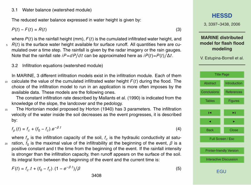
3.1 Water balance (watershed module)

The reduced water balance expressed in water height is given by:

P (t) − F (t) = R(t) (3)

where P (t) is the rainfall height (mm), F (t) is the cumulated infiltrated water height, andR(t) is the surface water height available for surface runoff. All quantities here are cu-5

mulated over a time step. The rainfall is given by the radar imagery or the rain gauges.Note that the rainfall rate iP=dP/dt can be approximated here as iP (t)=P (t)/∆t.

3.2 Infiltration equations (watershed module)

In MARINE, 3 different infiltration models exist in the infiltration module. Each of themcalculate the value of the cumulated infiltrated water height F (t) during the flood. The10

choice of the infiltration model to run in an application is more often imposes by theavailable data. These models are the following ones.

The constant infiltration rate described by Mallants et al. (1990) is indicated from theknowledge of the slope, the landcover and the pedology.

The Hortonian model proposed by Horton (1940) has 3 parameters. The infiltration15

velocity of the water inside the soil decreases as the event progresses, it is describedby:

fp (t) = fc + (f0 − fc).e−β.t (4)

where fp is the infiltration capacity of the soil, fc is the hydraulic conductivity at satu-ration, f0 is the maximal value of the infiltrability at the beginning of the event, β is a20

positive constant and t the time from the beginning of the event. If the rainfall intensityis stronger than the infiltration capacity, then runoff appears on the surface of the soil.Its integral form between the beginning of the event and the current time is:

F (t) = fc.t + (f0 − fc) .(1 − e−β.t)/β (5)

3408





HESSD3, 3397–3438, 2006


modeling


Title Page



Tables Figures

J I

J I

Back Close

Full Screen / Esc



EGU

where F (t) is the cumulated water height infiltrated. If the rainfall rate is smaller thanthe infiltration capacity (rate), then this infiltrated water height should be numericallycorrected with the introduction of an artificial equivalent time. The resolution of thisequation in MARINE is upstream time explicit.

In the Green and Ampt model, once the pounding time has been reached, the infil-5

tration capacity (rate) is modeled by:

fp(t) = K.[

1 +(θs − θi ).Sf

F (t)

](6)

where K is the hydraulic conductivity, Sf is the wetting front suction, θs is the saturatedwater content or porosity of the soil (also denoted Φ), θi the initial water content, and Fthe total water height infiltrated. The resolution of this equation in MARINE is upstream10

time explicit if the pounding time is neglected and implicit in the case of poundingprocess.

3.3 Runoff equations (watershed module)

Once the runoff water height is evaluated (R(t)), it is transferred all over the hill slopes,with one of the two proposed rooting methods presented bellow.15

The first one method consists on a direct resolution of the cinematic wave approx-imation. The water is supposed to be uniformly distributed over a pixel and its localvelocity (U) is approached by:

|U | =h

23n

n.√|I | (7)

Where U is the velocity (m/s), n is the Manning coefficient (m−1/3.s), hn is the uniform20

water height on the soil (m) and I is the local slope of the hill slope (m/m).The resolution is realized with an eulerian approach solving the mass balance for

each pixel of the model discretised over the grid of the DEM with an explicit upstream

3409





HESSD3, 3397–3438, 2006


modeling


Title Page



Tables Figures

J I

J I

Back Close

Full Screen / Esc



EGU

scheme:

∆mi +∑j=1,4

vj .nj

mj

dx∆t =R(t) × dx2 (8)

where i is the current pixel and j one of the 4 adjacent pixels, dx is the scale of thepixel and n is the outside direction of the pixel side. Recall that R(t) is the water heightavailable for runoff, accumulated over a time step ∆t, as defined in Eq. (3).5

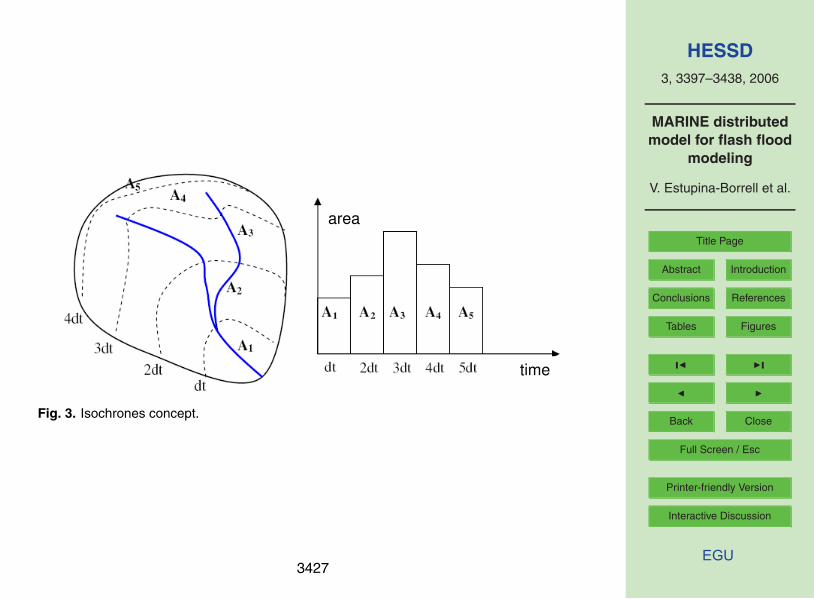
The second way of estimating surface runoff (in our model) is by using the conceptof variable isochrones (see Fig. 3).

The solution method is lagrangian, considering each one of the pixels of the DEMgrid.

Classically the hypothesis of the isochrones and unit hydrograph concepts are uni-10

form rain, global behavior of the basin and linear rainfall-runoff relation. In the method-ology developed here, some of them have been relaxed: heterogeneities of rain can betaken into account, heterogeneities of the topography and land cover are consideredand rainfall-runoff relation is based on cinematic wave velocity. Considering the mostcomplete resolution, the water depth over each pixel should be calculated at each time15

step, but the estimation of this last value is too much time consuming in calculationfor real time conditions. The optimal solution adopted here consists on making a bal-ance at the pixel scale to evaluate an equivalent potential local water depth (Fig. 4 andEq. 9).

hi j =

IP ij .Sssbvij .ni j√Ii j .li j

35

(9)

20

where hi j is the equivalent potential water depth on the pixel, IP ij is the rain intensity,Sssbvij is the area of the sub-basin upstream the pixel, ni j is the Manning coefficient,I i j is the local slope and l i j is the stream flow width. This expression is used in the

3410





HESSD3, 3397–3438, 2006


modeling


Title Page



Tables Figures

J I

J I

Back Close

Full Screen / Esc



EGU

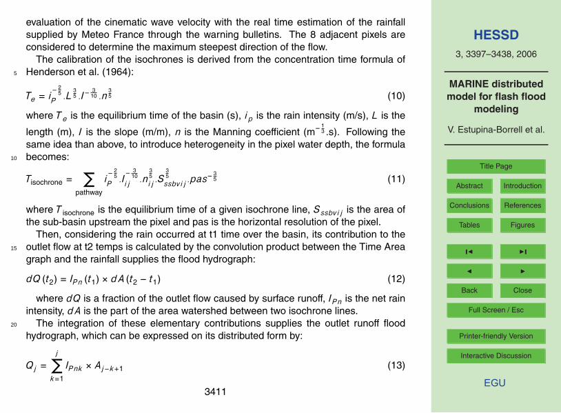
evaluation of the cinematic wave velocity with the real time estimation of the rainfallsupplied by Meteo France through the warning bulletins. The 8 adjacent pixels areconsidered to determine the maximum steepest direction of the flow.

The calibration of the isochrones is derived from the concentration time formula ofHenderson et al. (1964):5

Te = i− 2

5

P .L35 .I−

310 .n

35 (10)

where T e is the equilibrium time of the basin (s), ip is the rain intensity (m/s), L is the

length (m), I is the slope (m/m), n is the Manning coefficient (m− 13 .s). Following the

same idea than above, to introduce heterogeneity in the pixel water depth, the formulabecomes:10

Tisochrone =∑

pathway

i− 2

5

P .I− 3

10

i j .n35

i j .S35

ssbvij .pas− 3

5 (11)

where T isochrone is the equilibrium time of a given isochrone line, Sssbvij is the area ofthe sub-basin upstream the pixel and pas is the horizontal resolution of the pixel.

Then, considering the rain occurred at t1 time over the basin, its contribution to theoutlet flow at t2 temps is calculated by the convolution product between the Time Area15

graph and the rainfall supplies the flood hydrograph:

dQ (t2) = IP n (t1) × dA (t2 − t1) (12)

where dQ is a fraction of the outlet flow caused by surface runoff, IP n is the net rainintensity, dA is the part of the area watershed between two isochrone lines.

The integration of these elementary contributions supplies the outlet runoff flood20

hydrograph, which can be expressed on its distributed form by:

Qj =j∑

k=1

IP nk × Aj−k+1 (13)

3411





HESSD3, 3397–3438, 2006


modeling


Title Page



Tables Figures

J I

J I

Back Close

Full Screen / Esc



EGU

where Qj is the outlet flow at time j (coinciding with t2), Ipn is the net rain intensity,A is the watershed area between isochrone (j−k+1) and isochrone (j−k).

The use of the concept of variable isochrones, instead of the direct resolution of thecinematic wave approximation, leads us to consider that the infiltration is effective onlyat the rainfall location, and as a consequence, it leads us to neglect “re-infiltration”5

phenomena. According to Moore et al. (1990) and Carluer (1998), this approximationcan lead to an error of at most 10% on the rising curve of the flash flood hydrograph.

In both cases (concept of variable isochrones and direct resolution of the cinematicwave approximation), the 2-D basin runoff module supplies important flow data for thepixels that are outlets to the stream network, e.g. pixels coinciding with the outlet of10

temporary or permanent tributaries to the main river.

3.4 River propagation equations (stream network module)

The propagation inside the river is performed by solving the complete Saint Venantequations, which can be expressed as follow (taking into account a lateral input flow inthe continuity equation):15

∂S∂t + ∂Q

∂x = qlat∂Q∂t + ∂(Q2/S)

∂x + gS ∂H∂x = gS(I − J) + kqlat

QS

(14)

where S is the cross section of the river, qlat is the lateral flow from the tributaries ofthe main river (output of the hydrologic watershed module), supplied by the watershedmodule of MARINE, x is the coordinate along the river, Q is the river flow, t the time, Hthe water height of the river, I its topographic slope and J is energy slope.20

The solution of these equations is performed by the MAGE 1-D code (CEMAGREFsoftware, presented by Guiraudet al., 1997).

3412





HESSD3, 3397–3438, 2006


modeling


Title Page



Tables Figures

J I

J I

Back Close

Full Screen / Esc



EGU

4 Application and test of the model: the 1999 flash flood at Lagrasse (Aude,France)

MARINE has been tested for the flash flood of the Orbieu river basin on the 12 and 13of November 1999. The area of the basin is about 250 km2 upstream from Lagrassevillage. The sub-basin of interest (Orbieu) is part of the mediterranean Aude basin5

(4840 km2) in southern France. The Orbieu river is the main tributary of the Aude river,it drains the northern part of the Corbieres mountains. Fore more detailed informationon this flash flood, the reader is referred to Gaume et al. (2004).

4.1 Basin description and data

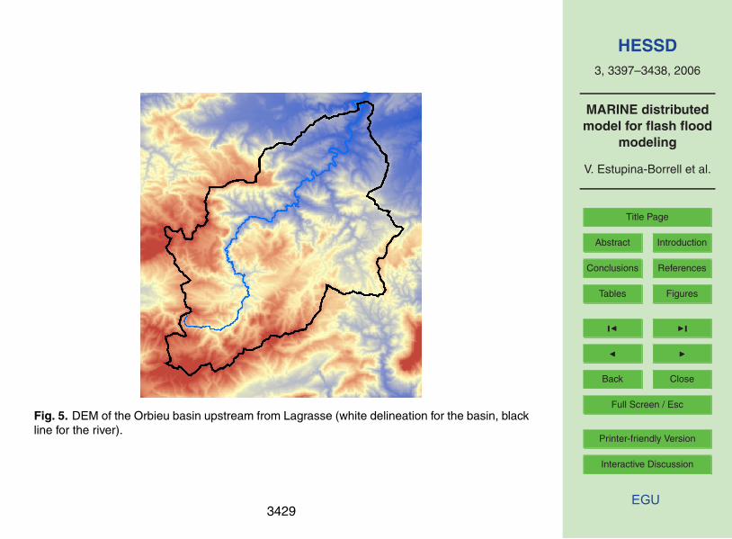
The Digital Elevation Model (DEM) is extracted from the BD IGN with a spatial resolu-10

tion of 50 m (Fig. 5) and the land cover map is interpreted from a LANDSAT TM image(Fig. 6). The soil is mainly sandy clay loam.

For this event, we have the data of three rain gauges located inside the basin (Fig. 7).The Thiessen repartition of the rain gauges was implemented. Maximal rainfall inten-sity is 60 mm/h, its duration is about 1.5 days and the cumulative rain on the basin is15

between 300 and 400 mm (Fig. 8). The cumulated rainfall observed with the meteoro-logical radar gives more information about the rainfall location (Fig. 9).

The river water elevation observed gives information on the flows that occurred atLagrasse (Fig. 10), but this indication is full of uncertainties because of the necessaryextrapolation of the stage discharge relationship and of the observations themselves20

(sediments, debris and instrumentation).

4.2 Optimal resolution of distributed (rainfall and DEM) data

In this section, we analyze the best possible choices concerning the resolution of dis-tributed space(-time) data, along with the chosen decomposition between the “basin”and “stream network” sub-domains. The spatially distributed data differ from the more25

3413





HESSD3, 3397–3438, 2006


modeling


Title Page



Tables Figures

J I

J I

Back Close

Full Screen / Esc



EGU

classical hydrologic observations (and from the needed inputs of the hydrological equa-tions) in theme, spatial and temporal resolutions and in precision. That’s why a specificwork has to be done concerning the resolution of the distributed field of data and theprocess to model.

Sensitivity tests realized on different DEM resolutions (∆xDEM) show that the maxi-5

mal resolution of DEM for hydrological applications with MARINE on the Orbieu basinis about 100 m (above this threshold, the precision of the information is not fine enoughto determine faithful runoff pathways).

The autocorrelogram study of the available DEM (the autocorrelation function sup-plies a common approach to investigating the effect of a nonlinear scalar transformation10

on a strongly stationary time series by representing the dependence between a pair ofvariables) confirms the hypothesis that a resolution between 100 m and 150 m couldbe enough (Fig. 11).

The minimal distributed data resolution is not defined by these methodologies, butthe equations used to characterize processes (cinematic wave approximation in this15

case) is validate for a maximum step between the input data resolution and the basinscale. Choosing very precise data will conduce to define a sub-model to treat them.

To conclude this part, for the watershed under study, the input pixel scale of MARINEis evaluated by 2 different methodologies and comforted by the literature between a fewten meters to about hundred meters. Since the available data have a 50 m resolution,20

this pixel size will be used for the study (the detailed study dealing with horizontalresolution and vertical accuracy is presented in Estupina-Borrell (2004).

The decomposition between the two modules of MARINE (hydrological runoff on hillslopes, and hydraulic flood propagation in the rivers) were defined by applying criteriato the spatially distributed dimensionless numbers “F ” and “k” presented earlier (Eqs. 125

and 2). In the specific case of the Orbieu basin, we obtain the decomposition in 2 sub-domains as shown in Fig. 11 below (white regions versus dark regions). To apply thecriteria, we used a rough a priori estimation of the water height over the basin based onthe rainfall rates forecasted in the official warning bulletins (30 mm/h in Eq. (11). The

3414





HESSD3, 3397–3438, 2006


modeling


Title Page



Tables Figures

J I

J I

Back Close

Full Screen / Esc



EGU

dark regions represent the pixels of the watershed where our criteria forbid the use ofthe cinematic wave approximation. One can observe that these computed dark pixelsactually match fairly well the main river and a few of its tributaries. The hydraulic streamflow module of Marine will be used for these pixels. Precise that there is no specifictreatment in this study, the only one treatment is the one realized on the DEM for the5

lagragian resolution presented part 2.2. The hydrographic network appears from theDEM and the spatial distribution of “F ” an “k” only (Fig. 12).

This delineation is obtained for a DEM pixel size of 50 m. In the case of a 100 mresolution, the delineation between watershed and stream flow modules would havealmost been the same.10

The data to get should have a resolution of about 50 m, but once the pretreatmentof MARINE done it is possible to define a data pixel size with a rougher resolution forMARINE resolution (until 1000 m).

4.3 Sensitivity of model with respect to initial water content

Different sensitivity tests on the initial soil water content condition for flash floods show15

that this initial condition is not as important as it is for other kind of floods (Fig. 13).They put in evidence that, in our context and in front of the existing uncertainties onthe observations and rainfall, it is acceptable to work on a discrete field of initial watercontent values: 0, 25, 50, 75, 100%.

For the Green and Ampt model, it can be explained by the fact that the pounding20

time is quite short because of the important rainfall intensities from the very start ofthe event. So the effective infiltration rate is the potential infiltrability of the soil. In thiscase, more the effective hydraulic conductivity is important, more the infiltrated volumerapidly increases and less the initial value of the soil humidity influences.

Even if the surface soil water content of the soil can be access from spatial tech-25

niques, it can not be faced to integrate this information in a real time context. Ourmethodology is based on a simplified assimilation technique. It consists in followingthe 5 possible hydrographs, each one with characteristic soil water content (0%, 25%,

3415





HESSD3, 3397–3438, 2006


modeling


Title Page



Tables Figures

J I

J I

Back Close

Full Screen / Esc



EGU

50%, 75%, 100%), and the real time observations of the outlet flow to choice the wellfitted initial condition between the 5 tested. This operation is done only on the firsttime steps of the floods during the rising curve until the level of alarm of the river isreached. Initial soil water content (or more generally the initial saturation state of thewatershed, including both soil water content and depth of shallow groundwater) is an5

open problem, still being explored. . . Moreover, the relatively slow evolutions of sub-surface moisture and water table may not be as important for the type of flash floodsinvestigated here, as they would be for slower types of floods.

4.4 Calibration and data assimilation

Vieux et al. (2004) demonstrates that physically based distributed models, which are10

formulated to make runoff predictions using parameters derived form physically water-shed properties, can be a priori calibrate with geospatial data only (terrain, soil, landcover). Even if this calibration would be improve using past rain and flow observations,a limited number of events could allow to converge towards an optimal calibration (in-cluding more events materially does not change the calibration).15

In this case, in front of the lack of past observed events, the parameters of MARINEare the geospatial derived one. They could be adjusted to counterbalance the hypoth-esis of homogeneity of the model pixel done for the upscaling or to take into accountthe different uncertainties on the data or approximations of the model, but this stagewould need other observations of flash floods on this watershed.20

The Manning coefficients on the hillslopes are interpreted thanks to its tabulatedvalues proposed by Chow (1959) from the land cover map. For example, as is the casehere for the Orbieu watershed, a vegetation cover comprising dense trees over 70% ofits area is represented, hydraulically, by a Manning coefficient n ≈0.1 SI.

The hydraulic roughness of the main channel was estimated, thanks to in situ ob-25

servations of the river bed, the Manning hydraulic roughness coefficient (“n”) of themain channel was between 0.05 to 0.1 SI (the equivalent Stikler hydraulic roughnesscoefficient was between 10 to 20 SI).

3416





HESSD3, 3397–3438, 2006


modeling


Title Page



Tables Figures

J I

J I

Back Close

Full Screen / Esc



EGU

The soil texture class is clay loam and sandy clay loam. The corresponding constantinfiltration rate is 0.5. The Horton parameters are fixed in accordance with a loamysoil and with the Holtan model (fo=4*fc) and β at 0.1 min–1. The matching Green andAmpt infiltration parameters are a porosity of 0.464 and 0.398, a wetting front soil of0.2088 m and 0.2185 m (these values are the ones proposed by Maidment (1993)).5

The calibrations of saturated hydraulic conductivity and of the initial water contentof the soil are realized step by step with the simplified data assimilation techniquepresented above during the first hours of the flood. For the Horton infiltration ratemodel, this procedure yields an infiltration rate capacity (fc) of 1.5 mm/h, and for theGreen and Ampt model, an initial soil water content of 0% and a saturated hydraulic10

conductivity of 1.5 mm/h.

4.5 Rainfall estimation and spatialisation

First, let us define “spatialisation”. Spatialisation can be understood here as estimation,interpolation, extrapolation of rainfall in (x,y) space; also the problem of aggregatingor disaggregating rainfall on the desired pixel sizes (e.g.: from ∆×RAIN to ∆×DEM);15

and finally, the problem of taking into account temporal resolution (particularly for non-stationary storms).

For instance, Tetzlaff et al. (2005) demonstrates the considerable importance of rain-fall spatialisation and its consequence on the basin response (hydrographs) dependingon the kind of storm/flood event being studied.20

In the case at hand, we have only 3 rain gauges and some cumulated rain radarimages, but nevertheless, some of our tests (not all described here) indicate that theyprovide a sufficiently reasonable (robust) representation of the space-time rainfall pat-tern. Furthermore, the temporal resolution used in this specific case for rainfall is quiteprecise (∆tRAIN=15 min). But the extremely heterogeneous character of rainfalls gen-25

erating such a flash flood may not be not correctly reproduced in the input data usedand so may generate some uncertainties.

3417





HESSD3, 3397–3438, 2006


modeling


Title Page



Tables Figures

J I

J I

Back Close

Full Screen / Esc



EGU

5 Application and test of the model: simulation results and discussion

5.1 Flash flood simulation results: flood hydrographs

The results of the simulations obtained with Marine for the Lagrasse flash flood ofNovember 1999 on the Orbieu basin, are presented and discussed in this section(Fig. 14).5

Gaume et al. (2004) explain that this specific flood is mainly due to fast respondinghydrological processes, the reactivity of the watershed to fluctuations in rainfall intensityis important. Indeed, the first observed hydrograph peak (about 550 m3/s) is producedby the pluviograph peak observed at Lagrasse. The third observed hydrograph peak(about 220 m3/s) is probably due to the pluviograph peak observed at Bouisse (11 h10

later than the one of Lagrasse plus the delay time due to the time routing of the waterbetween upstream and dowstream parts of the basin). But the second hydrograph peak(about 350 m3/s) can not find explanation within the rainfall data available. Furthermorethe very rapid decreasing and rising of the flow may reforce the thesis of errors on waterelevation measurements in the river bed or wrong interpretation of them (debris).15

The study of Gaume et al. (2004) of the same flood that occurred on a smallerneighborhood basin shows (among all) that the amount of losses by infiltration for thisflood is about 200 mm and occurred mainly at the beginning of the event. Furthermore,it supposes that the type of land cover of the basin is of second importance during thisevent.20

The present study confirms these points:

– The calibrated infiltration coefficient, regardless of the type of infiltration modelbeing used, shows that a considerable part of the rain was stored in the soilduring this flood (from 100 to 200 mm).

– The behavior of the woody watershed of this study seems to be equivalent in lots25

points of the watershed mainly occupied by vineyards and scrubs of the precedent

3418





HESSD3, 3397–3438, 2006


modeling


Title Page



Tables Figures

J I

J I

Back Close

Full Screen / Esc



EGU

study. This observation confirms the hypothesis as the type of land use seems tobe of second importance during this event.

5.2 Discussion of simulated vs. observed flood hydrographs

The results of the simulations realized with the different modules of MARINE are quitesimilar in their global form and timing, but their amplitude can be different.5

The rising curve of the first observed hydrograph peak (about 550 m3/s), the reces-sion curve of the second observed flood hydrograph peak (about 350 m3/s) and thethird observed hydrograph peak (about 220 m3/s) are comprised between the upperand the lower envelopes defined by the different simulations.

Two parts of the observed hydrograph: the second observed peak (about 350 m33/s)10

(probably wrong, see just below) and the end part of the recession curve of the hydro-graph (the recession curve of the third peak of about 220 m3/s). The second mismatchcan be explained by the observed rain data used for the simulation. The three precipi-tation gauges spatialised and corrected with a Thiessen repartition and with the radarmeteorological cumulated precipitation data do not supply very satisfactory precipita-15

tion field.One can observe that the infiltration module with the constant rate supplies quite

good results for real time forecasting. For the Horton concept, this can be explainedby the fact that in less than one hour, the value of the exponential term of the equationbecomes negligible compared to the value of the saturated hydraulic conductivity (fc).20

So this model quickly behaves like a constant one. For the Green and Ampt model, thebehavior of the simulated hydrograph is quite different. It first presents a delay in thestarting point of the rising curve compared with the constant rate model and the Hortonmodel, and than it presents a more rapid rising curve.

Admittedly, these results could have be improved by a direct calibration of the model25

on the observed flash flood hydrograph, but this methodology does not enter within theframework of our research.

3419





HESSD3, 3397–3438, 2006


modeling


Title Page



Tables Figures

J I

J I

Back Close

Full Screen / Esc



EGU

6 Conclusions

MARINE was formulated to make flash floods prediction caused by surface runoff pro-cess. In front of the rareness, violence and rapidity of flash floods, MARINE had tofind its necessary data for calibration outside the classical measurements and obser-vations.5

That is the reason why MARINE is a physically based hydrological distributed model.Its physically distributed character allows the a priori calibration of its most parameters.The remotely sensed data can be used for this goal. Some adaptations specific to thehydrology field have to be done and more particularly the scale of definition of theseimages has to be taken into account. Then spatial DEMs or land cover maps can be10

used as data for flash flood forecasting.Another important issue concerns the calibration (or data assimilation) of the model

with respect to the initial saturation state of the basin. In this case, we have adjustedthe initial conditions (initial water content in the soil) or other sensitive parameters (hy-draulic conductivity of the soil) with the first observed flow at the outlet of the basin15

(until the level of alert is reached). But, more generally, this issue is open and coupledwith the equifinality issue; some more investigations have to be realized to improve thistechnique (keeping in mind the necessary rapidity of the model to use).

Nevertheless the results obtained on the flash flood of November 1999 in the south-ern France indicate that this particular model is able to reproduce the hydraulic behavior20

of the watershed.Furthermore, the MARINE model was initially designed for real time forecasting,

implying the following constraints:

– Sufficiently short computational time (CPU time);

– Data requirements compatible with the type of data actually available in real time;25

– Model results (model outputs) formulated in accordance with the forecaster’sneeds.

3420





HESSD3, 3397–3438, 2006


modeling


Title Page



Tables Figures

J I

J I

Back Close

Full Screen / Esc



EGU

MARINE is the formulation of a relatively basic physical approach with adequate nu-merical method. This particularity makes this model conform to the objectives of fore-casting flash floods with a sufficient precision.

To test its applicability in real time conditions, MARINE was introduced inside thePACTES project by Alquier et al. (2002). PACTES started in January 2000 for a two5

years pre-operational application project. It was lead by the French Ministry of Re-search and the French Space Agency CNES. PACTES traduces the will to improve themanagement of the flooding risk over its different phases (prevention, early warning,crisis and post-crisis). It is a transverse and multi-disciplinary operation which asso-ciates the operational users (Civil Protection, Flood Warning Services, regional land10

planning services), the meteorological and hydrological researchers and the space in-dustry.

The objectives of this project are to integrate advanced modeling techniques, to usespace techniques, to combine different sources of information for decision support,and to allow the different actors to share information and to exchange it in real-time15

during alert and crisis phases. This project leads to development of a pre-operationaldemonstrator which is a distributed information system, based on GIS and Internettechnologies. It was applied on the French watershed of the Thore river, in the Tarndepartment. First back up from this experience show that MARINE is adapted to thereal time operational forecasting conditions.20

Acknowledgements. This research was carried out at the Institute of Fluid Mechanics ofToulouse (IMFT). The authors are particularly grateful for the help provided by the IMFT Sur-face Hydrology team. The authors would also like to thank C. Puech at the “Maison de laTeledetection” in Montpellier, J. M. Tanguy at the SCHAPI in Toulouse, the SCOT companyin Toulouse for their technical and financial support, and the DDE-11 who provided some of25

the data used in this study. Finally, the authors extend their thanks to every partner and dataprovider of the PACTES research project, namely: ADAGE Dvpt, Alcatel Space Industries, AS-TRIUM, BRGM, CEMAGREF, Civil Security, CNES, EADS S&DE, Flood Alert Services, FrenchMinistry of Research, French Ministry of Environment, IGN, IMFT, IRIT, Meteo France, SERTIT,SCOT and SPOT Image.30

3421





HESSD3, 3397–3438, 2006


modeling


Title Page



Tables Figures

J I

J I

Back Close

Full Screen / Esc



EGU

References

Ababou, R. and Tregarot, G., Coupled Modeling of Partially Saturated Flows: Macro-PorousMedia, Interfaces, and Variability. Proc. CMWR 2002: Comput. Methods in Water Resources(23–28 June 2002, Delft, The Netherlands), Comput. Mech. Publi, 8pp, 2002.

Albergel, J.: Le modele hortonien: genese des crues et des inondations, Ed. SHF, Paris, EN-5

GREF, 10–15, 2003.Alquier, M., Chorda, J., Dartus, D., Estupina Borrell, V., Llovel, C., and Maubourguet, M. M.:

PACTES: La chaıne de prevision du Thore, Research Contract, IMFT, Toulouse, 2002.Booij, M. J.: Appropriate modelling of climate change impacts on river flooding, Twente, 206pp,

2002.10

Borgniet, L., Estupina-Borrell, V., Dartus, D., and Puech., C.: Methodologies for analyzingintrinsic and required DEM accuracy for hydrological applications of flash floods. CanadianJournal of Remote Sensing. Special collection: Applications of remote sensing in hydrology,29(6), 734–740, 2003.

Bousquet, J. C.: Geologie du Languedoc Roussillon, Les presses du Languedoc, Editions du15

BRGM, 1997.Carluer, N.: Vers une modelisation hydrologique adaptee a l’evaluation des pollutions diffuses:

prise en compte du reseau anthropique, Pierre et Marie Curie, Lyon, 386pp, 1998.Chahinian, N., Moussa,, R., Andrieux, P., and Voltz. M.: Comparison of infiltration models to

simulate flood events at the field scale, J. Hydrol., 306(1–4), 191–214, 2005.20

Chow, V. T.: Open Channel Hydraulics edited by: Davis, H. E. (consulting Editor), 680pp, 1959.Cosandey, C. and Robinson, M.: Hydrologie continentale, Armand Colin, Paris, 360 p., 2000,Datin, R.: Outils operationnels pour la prevision des crues rapides: traitement des incerti-

tudes et integration des previsions meteorologiques, Developpements de TOPMODEL pourla prise en compte de la variabilite spatiale de la pluie. Application au bassin versant de25

l’Ardeche, These INPG, Grenoble, 266pp, 1998.Estupina-Borrell, V. and Dartus, D.: La telede-tection au service de la prevision operationnelle

des crues eclair, Bulletin de la Societe Francaise de Photogrametrie et de Teledetection, 4,31–39, 2003.

Estupina, V., Llovel, C., Maubourguet, M. M., Chorda, J., Dartus, D., Ababou, R., and Alquier,30

M.: Flash Flood Modeling for Prediction, Warning and Risk Assessment. In: Trends derWasserwirtschaft 33.IWASA Internat, Wasserbau-Symposium, Aachen 2003, RWTH Univ.

3422





HESSD3, 3397–3438, 2006


modeling


Title Page



Tables Figures

J I

J I

Back Close

Full Screen / Esc



EGU

Aachen, Institut Wasserbau & Wasserwirtschaft: Mitteilunge, Shaker Verlag, Aachen ISBN3-8322-3083-1, Germany, 175–223, 2004.

Estupina-Borrell, V.: Vers une Modelisation Hydrologique adaptee a la Prevision Operationnelledes Crues Eclair – Application a de Petits Bassins du Sud de la France, These INPT,Toulouse, , 241p, 2004.5

Estupina-Borrell, V., Chorda, J., and Dartus, D.: Flash floods anticipation / Prevision des crueseclair, Comptes rendus Geosci., 337, 13, 1109–1119, 2005.

Foody, G. M., Ghoneim, E. M., and Arnell, N. W.: Predicting locations sensitive to flash floodingin an arid environment, J. Hydrol., 292, 1–4, 48–58, 2004.

Gaume E., Livet, M., Desbordes, M., and Villeneuve., J. P.: Hydrological analysis of the rver10

Aude, France, flash flood on 12 and 13 Novembre 1999, J. Hydrol., 286, 1–4, 135–154, 2004.Giraud, F., Faure, J. B., Zimmer, D., Lefeuvre, J. C., and Skaggs, R. W.: Modelisation hy-

drologique d’une zone humide complexe, J. irrigation, 123(5), 1531–1540, 1997.Henderson, F. and Wooding, R.: Overland flow and groundwater from a steady rainfall of finite

duration, J. Geophys. Res., 69(8), 1531–13 540, 1964.15

Horton, R. E.: An approach toward a physical interpretation of infiltration-capacity, Soil Sc. Soc.Am., 5, 399–417, 1940

IAHS, UNESCO, WMO: Flash floods,Proceedings of the Paris symposium, edited by: IAHS-UNESCO-WMO, 112, 1974.

Liu, Z. and Todini, E.: Towards a comprehensive physically-based rainfall runoff model, Hydrol.20

Earth Syst. Sci., 6(5), 859–881, 2002.Maidment, D. R.: Handbook of Hydrology, Publisher: McGraw-Hill Professional, 1424, 1993,Mallants, D. and Feyen, J.: Quantitative and qualitative aspects of surface and groundwater

flow, 2, KUL, 96, 1990Meentemeyer, V.: Geographical perspectives of space, time and scale, Landscape Ecology., 3,25

163–173, 1989.Montz, B. E. and Gruntfest, E.: Flash flood mitigation: recommandations for research and

applications, Environ-mental Hazards, 1–15, 2002.Moore, I. D. and Foster, G. R.: Hydraulics and overland flow, Process studies in hillslope re-

search, edited by: Anderson, M. G. and Burt, T. P., John Wiley and sons, 215–254, 1990.30

Puech, C.: Utilisation de la teledetection et des modeles numeriques de terrain pour la connais-sance du fonctionnement des hydrosystemes, UMR35, CEMAGREF ENGREF, Montpellier,2000.

3423





HESSD3, 3397–3438, 2006


modeling


Title Page



Tables Figures

J I

J I

Back Close

Full Screen / Esc



EGU

Rodriguez-Iturbe, I., Mejia, J. M.: On the transformation from point rainfall to areal rainfall.Water Resour. Res., 10 (4), 729–735, 1974.

Sivapalan, M. and Bloschl, G.: Transformation of point rainfall to areal rainfall: Intensity-duration-frequency curves, J. Hydrol., 204(1–4), 150–167, 1998.

Tetzlaff, D. and Uhlenbrook, S.: Significance of spatial variability in precipitation for process-5

oriented modelling: results from two nested catchments using radar and ground station data,Hydrol. Earth Syst. Sci., 9, 29–41, 2005.

Vieux, B. E., Cui, Z., and Gaur, A.: Evaluation of a physics-based distributed hydrologic modelfor flood forecasting, J. Hydrol., 298, 1–4, 155–177, 2004.

Walsh, S. J., Crawford, T. W., Welsh, W. F., and Crews-Meyer, K. A.: A multiscale analysis of10

LULC and NDVI variation in Nang Rong district, northeast Thailand, Agriculture, Ecosyst.Environment., 85(1–3), 47–64, 2001.

3424





HESSD3, 3397–3438, 2006


modeling


Title Page



Tables Figures

J I

J I

Back Close

Full Screen / Esc



EGU

Page 7

under ground transfers are characterized by transfer times which are not of the same scale order than those

of flash flood processes for the basins of interest.

Figure 1. General flow-chart of the MARINE hydrological model

DEM treatments

The DEM is the data which supplies the information on water trajectories over the surface. This data should

be able to determine the position of the permanent and temporary tributaries of the main river of the basin.

Like all DEMs, it contains holes and peaks. The DEM treatment of MARINE proposed by Estupina and al.

(2004) consists on first identifying them and then treating them with a procedure inspired from GIS

techniques. The determination of the optimal water paths is done from the original DEM, finding the

steepest descent on an increasing neighborhood. According to the runoff resolution (eulerian or lagrangian)

Fig. 1. General flow-chart of the MARINE hydrological model.

3425





HESSD3, 3397–3438, 2006


modeling


Title Page



Tables Figures

J I

J I

Back Close

Full Screen / Esc



EGU

Diffusion

approximation

Kinematic

approximation

Saint Venant Equations

FL Froude Number

K N

um

ber

of

kin

em

ati

cfl

ow

Fig. 2. Validity of the cinematic wave approximation according to Moore et al. (1990).

3426





HESSD3, 3397–3438, 2006


modeling


Title Page



Tables Figures

J I

J I

Back Close

Full Screen / Esc



EGU

area

time

Fig. 3. Isochrones concept.

3427





HESSD3, 3397–3438, 2006


modeling


Title Page



Tables Figures

J I

J I

Back Close

Full Screen / Esc



EGU

h

lrigole

Sssbv

P

u

Fig. 4. Balance for the blue pixel size (Sssbv: area of the basin upstream the pixel, u: watervelocity on the pixel, lrigole: width of the “channel” draining water, h: water depth on the pixel).

3428





HESSD3, 3397–3438, 2006


modeling


Title Page



Tables Figures

J I

J I

Back Close

Full Screen / Esc



EGU

Fig. 5. DEM of the Orbieu basin upstream from Lagrasse (white delineation for the basin, blackline for the river).

3429





HESSD3, 3397–3438, 2006


modeling


Title Page



Tables Figures

J I

J I

Back Close

Full Screen / Esc



EGU

Fig. 6. Landcover map of the Orbieu basin upstream from Lagrasse (70% of wood (green),17% of grassland (ligth green), 12% of vigneyards (violet), others (1.2%)).

3430





HESSD3, 3397–3438, 2006


modeling


Title Page



Tables Figures

J I

J I

Back Close

Full Screen / Esc



EGU

Fig. 7. Location of the pluviographs: North: Lagrasse, East: Mouthoulet, West: Bouisse.

3431





HESSD3, 3397–3438, 2006


modeling


Title Page



Tables Figures

J I

J I

Back Close

Full Screen / Esc



EGU

Rainfall - Aude November 1999

0

10

20

30

40

50

60

1 11 21 31 41 51 61 71 81 91 101 111 121 131 141 151 161 171

time from the 12/11/99 at 00h (dt=15 min)rain

(m

m/h

)

Bouisse

Lagrasse

Mouthoumet

Fig. 8. Bouisse, Moutoumet and Lagrasse pluviographs (rain in mm/h).

3432





HESSD3, 3397–3438, 2006


modeling


Title Page



Tables Figures

J I

J I

Back Close

Full Screen / Esc



EGU

Fig. 9. Cumulated rainfall (mm) observed with the meteorological radar for the flash flood of1999.

3433





HESSD3, 3397–3438, 2006


modeling


Title Page



Tables Figures

J I

J I

Back Close

Full Screen / Esc



EGU

Flash flood of November 1999 at Lagrasse (Orbieu river) with MARINE

model

0

100

200

300

400

500

600

700

1 6 11 16 21 26 31 36 41 46 51 56 61 66

Time (h+1)

Flo

w (

m3

/s)

Fig. 10. Observed Flood Hydrograph at Lagrasse.

3434





HESSD3, 3397–3438, 2006


modeling


Title Page



Tables Figures

J I

J I

Back Close

Full Screen / Esc



EGU

Fig. 11. Maximum pixel size defined by the autocorrelogram method.

3435





HESSD3, 3397–3438, 2006


modeling


Title Page



Tables Figures

J I

J I

Back Close

Full Screen / Esc



EGU

Fig. 12. Validity field of the cinematic wave approximation for the studied basin with a DEMpixel size of 50 m (black thick line: delineation of the basin, black fine points: excluded pointsfrom the field of validity, white area: field of validity of the cinematic wave approximation).

3436





HESSD3, 3397–3438, 2006


modeling


Title Page



Tables Figures

J I

J I

Back Close

Full Screen / Esc



EGU

Floood hydrograph of the Orbieu river at Lagrasse

Sensitivity of the initial water content of the soil (for a sandy clay loam soil)

with the Green&Ampt model

0

100

200

300

400

500

600

700

800

0 10 20 30 40 50 60 70

Time (h)

Flo

w (

m3

/s)

sol1 hum=0.389

sol1 hum=0.3

sol1 hum=0.2

sol1 hum=0.1

sol1 hum=0.0

Fig. 13. Influence of the initial water content of the soil on a flash flood hydrograph with a Greenand Ampt infiltration model.

3437





HESSD3, 3397–3438, 2006


modeling


Title Page



Tables Figures

J I

J I

Back Close

Full Screen / Esc



EGU

Flood hydrographs at Lagrasse

0

100

200

300

400

500

600

5 10 15 20 25 30 35 40 45 50 55 60 65

Time (h)

Flo

w (

m3

/s)

MARINE isoch var / CR=0.5

observations

MARINE isoch var / Horton fc=1.5mm/h

MARINE isoch var / G&A 1

MARINE isoch var / G&A 2

Fig. 14. Flood hydrographs at Lagrasse obtained with different infiltration modules of MARINE.

3438





v. estupina-borrell et al. - hessd - recent · 2016-01-10 · ing. this methodology should provide...

Documents