vaex documentationvaex documentation, release 3.0.0-dev warning: it is recommended not to install...
TRANSCRIPT

vaex DocumentationRelease 3.0.0-dev
Maarten A. Breddels
May 01, 2020


Contents
1 Short version 3
2 Longer version 5
3 For developers 7
4 Tutorials 94.1 Vaex introduction in 11 minutes . . . . . . . . . . . . . . . . . . . . . . . . . . . . . . . . . . . . . 94.2 Machine Learning with vaex.ml . . . . . . . . . . . . . . . . . . . . . . . . . . . . . . . . . . . . . 44
5 Examples 595.1 Arrow . . . . . . . . . . . . . . . . . . . . . . . . . . . . . . . . . . . . . . . . . . . . . . . . . . . 595.2 Dask . . . . . . . . . . . . . . . . . . . . . . . . . . . . . . . . . . . . . . . . . . . . . . . . . . . 685.3 GraphQL . . . . . . . . . . . . . . . . . . . . . . . . . . . . . . . . . . . . . . . . . . . . . . . . . 705.4 I/O Kung-Fu: get your data in and out of Vaex . . . . . . . . . . . . . . . . . . . . . . . . . . . . . 725.5 Machine Learning (basic): the Iris dataset . . . . . . . . . . . . . . . . . . . . . . . . . . . . . . . . 825.6 Machine Learning (advanced): the Titanic dataset . . . . . . . . . . . . . . . . . . . . . . . . . . . 87
6 API documentation for vaex library 1116.1 Quick lists . . . . . . . . . . . . . . . . . . . . . . . . . . . . . . . . . . . . . . . . . . . . . . . . 1116.2 vaex-core . . . . . . . . . . . . . . . . . . . . . . . . . . . . . . . . . . . . . . . . . . . . . . . . . 1126.3 Extensions . . . . . . . . . . . . . . . . . . . . . . . . . . . . . . . . . . . . . . . . . . . . . . . . 1706.4 Machine learning with vaex.ml . . . . . . . . . . . . . . . . . . . . . . . . . . . . . . . . . . . . . 206
7 Datasets to download 2277.1 New york taxi dataset . . . . . . . . . . . . . . . . . . . . . . . . . . . . . . . . . . . . . . . . . . 2277.2 SDSS - dereddened . . . . . . . . . . . . . . . . . . . . . . . . . . . . . . . . . . . . . . . . . . . . 2287.3 Gaia . . . . . . . . . . . . . . . . . . . . . . . . . . . . . . . . . . . . . . . . . . . . . . . . . . . . 2297.4 Helmi & de Zeeuw 2000 . . . . . . . . . . . . . . . . . . . . . . . . . . . . . . . . . . . . . . . . . 229
8 Frequently Asked Questions 2318.1 I have a massive CSV file which I can not fit all into memory at one time. How do I convert it to HDF5?2318.2 Why can’t I open a HDF5 file that was exported from a pandas DataFrame using .to_hdf? . . . 231
9 What is Vaex? 2339.1 Why vaex . . . . . . . . . . . . . . . . . . . . . . . . . . . . . . . . . . . . . . . . . . . . . . . . . 233
10 Installation 235
i

10.1 Getting started . . . . . . . . . . . . . . . . . . . . . . . . . . . . . . . . . . . . . . . . . . . . . . 235
11 Continue 239
Python Module Index 241
Index 243
ii

vaex Documentation, Release 3.0.0-dev
Warning: It is recommended not to install directly into your operating system’s Python using sudo since it maybreak your system. Instead, you should install Anaconda, which is a Python distribution that makes installingPython packages much easier or use virtualenv or venv.
Contents 1

vaex Documentation, Release 3.0.0-dev
2 Contents

CHAPTER 1
Short version
• Anaconda users: conda install -c conda-forge vaex
• Regular Python users using virtualenv: pip install vaex
• Regular Python users (not recommended): pip install --user vaex
• System install (not recommended): sudo pip install vaex
3

vaex Documentation, Release 3.0.0-dev
4 Chapter 1. Short version

CHAPTER 2
Longer version
If you don’t want all packages installed, do not install the vaex package. The vaex package is a meta packagesthat depends on all other vaex packages so it will instal them all, but if you don’t need astronomy related parts(vaex-astro), or don’t care about distributed (vaex-distributed), you can leave out those packages. Copypaste the following lines and remove what you do not need:
• Regular Python users: pip install vaex-core vaex-viz vaex-jupyter vaex-arrowvaex-server vaex-ui vaex-hdf5 vaex-astro vaex-distributed
• Anaconda users: conda install -c conda-forge vaex-core vaex-viz vaex-jupytervaex-arrow vaex-server vaex-ui vaex-hdf5 vaex-astro vaex-distributed
When installing vaex-ui it does not install PyQt4, PyQt5 or PySide, you have to choose yourself and installing maybe tricky. If running pip install PyQt5 fails, you may want to try your favourite package manager (brew, macports) toinstall it instead. You can check if you have one of these packages by running:
• python -c "import PyQt4"
• python -c "import PyQt5"
• python -c "import PySide"
5

vaex Documentation, Release 3.0.0-dev
6 Chapter 2. Longer version

CHAPTER 3
For developers
If you want to work on vaex for a Pull Request from the source, use the following recipe:
• git clone --recursive https://github.com/vaexio/vaex # make sure you get the submod-ules
• cd vaex
• make sure the dev versions of pcre are installed (e.g. conda install -c conda-forge pcre)
• install using:
• pip install -e . (again, use (ana)conda or virtualenv/venv)
• If you want to do a PR
• git remote rename origin upstream
• (now fork on github)
• git remote add origin https://github.com/yourusername/vaex/
• . . . edit code . . . (or do this after the next step)
• git checkout -b feature_X
• git commit -a -m "new: some feature X"
• git push origin feature_X
• git checkout master
• Get your code in sync with upstream
• git checkout master
• git fetch upstream
• git merge upstream/master
7

vaex Documentation, Release 3.0.0-dev
8 Chapter 3. For developers

CHAPTER 4
Tutorials
4.1 Vaex introduction in 11 minutes
Because vaex goes up to 11
4.1.1 DataFrame
Central to Vaex is the DataFrame (similar, but more efficient than a Pandas DataFrame), and we often use the variabledf to represent it. A DataFrame is an efficient representation for a large tabular dataset, and has:
• A number of columns, say x, y and z, which are:
• Backed by a Numpy array;
• Wrapped by an expression system e.g. df.x, df['x'] or df.col.x is an Expression;
• Columns/expression can perform lazy computations, e.g. df.x * np.sin(df.y) does nothing, until theresult is needed.
• A set of virtual columns, columns that are backed by a (lazy) computation, e.g. df['r'] = df.x/df.y
• A set of selections, that can be used to explore the dataset, e.g. df.select(df.x < 0)
• Filtered DataFrames, that does not copy the data, df_negative = df[df.x < 0]
Lets start with an example dataset, which is included in Vaex.
[1]: import vaexdf = vaex.example()df # Since this is the last statement in a cell, it will print the DataFrame in a→˓nice HTML format.
[1]: # id x y z vx→˓ vy vz E L→˓ Lz FeH0 0 1.2318683862686157 -0.39692866802215576 -0.598057746887207 301.→˓1552734375 174.05947875976562 27.42754554748535 -149431.40625 407.→˓38897705078125 333.9555358886719 -1.0053852796554565
(continues on next page)
9

vaex Documentation, Release 3.0.0-dev
(continued from previous page)
1 23 -0.16370061039924622 3.654221296310425 -0.25490644574165344 -195.→˓00022888183594 170.47216796875 142.5302276611328 -124247.953125 890.→˓2411499023438 684.6676025390625 -1.70866703987121582 32 -2.120255947113037 3.326052665710449 1.7078403234481812 -48.→˓63423156738281 171.6472930908203 -2.079437255859375 -138500.546875 372.→˓2410888671875 -202.17617797851562 -1.83361411094665533 8 4.7155890464782715 4.5852508544921875 2.2515437602996826 -232.→˓42083740234375 -294.850830078125 62.85865020751953 -60037.0390625 1297.→˓63037109375 -324.6875 -1.47868824005126954 16 7.21718692779541 11.99471664428711 -1.064562201499939 -1.→˓6891745328903198 181.329345703125 -11.333610534667969 -83206.84375 1332.→˓7989501953125 1328.948974609375 -1.8570483922958374... ... ... ... ... ...→˓ ... ... ... ...→˓ ... ...329,995 21 1.9938701391220093 0.789276123046875 0.22205990552902222 -216.→˓92990112304688 16.124420166015625 -211.244384765625 -146457.4375 457.→˓72247314453125 203.36758422851562 -1.7451677322387695329,996 25 3.7180912494659424 0.721337616443634 1.6415337324142456 -185.→˓92160034179688 -117.25082397460938 -105.4986572265625 -126627.109375 335.→˓0025634765625 -301.8370056152344 -0.9822322130203247329,997 14 0.3688507676124573 13.029608726501465 -3.633934736251831 -53.→˓677146911621094 -145.15771484375 76.70909881591797 -84912.2578125 817.→˓1375732421875 645.8507080078125 -1.7645612955093384329,998 18 -0.11259264498949051 1.4529125690460205 2.168952703475952 179.→˓30865478515625 205.79710388183594 -68.75872802734375 -133498.46875 724.→˓000244140625 -283.6910400390625 -1.8808952569961548329,999 4 20.796220779418945 -3.331387758255005 12.18841552734375 42.→˓69000244140625 69.20479583740234 29.54275131225586 -65519.328125 1843.→˓07470703125 1581.4151611328125 -1.1231083869934082
Columns
The above preview shows that this dataset contains > 300, 000 rows, and columns named x ,y, z (positions), vx, vy,vz (velocities), E (energy), L (angular momentum), and an id (subgroup of samples). When we print out a columns,we can see that it is not a Numpy array, but an Expression.
[2]: df.x # df.col.x or df['x'] are equivalent, but df.x may be preferred because it is→˓more tab completion friendly or programming friendly respectively
[2]: Expression = xLength: 330,000 dtype: float32 (column)---------------------------------------
0 1.231871 -0.1637012 -2.120263 4.715594 7.21719
...329995 1.99387329996 3.71809329997 0.368851329998 -0.112593329999 20.7962
One can use the .values method to get an in-memory representation of an expression. The same method can be
10 Chapter 4. Tutorials

vaex Documentation, Release 3.0.0-dev
applied to a DataFrame as well.
[3]: df.x.values
[3]: array([ 1.2318684 , -0.16370061, -2.120256 , ..., 0.36885077,-0.11259264, 20.79622 ], dtype=float32)
Most Numpy functions (ufuncs) can be performed on expressions, and will not result in a direct result, but in a newexpression.
[4]: import numpy as npnp.sqrt(df.x**2 + df.y**2 + df.z**2)
[4]: Expression = sqrt((((x ** 2) + (y ** 2)) + (z ** 2)))Length: 330,000 dtype: float32 (expression)-------------------------------------------
0 1.425741 3.666762 4.298243 6.952034 14.039...
329995 2.15587329996 4.12785329997 13.5319329998 2.61304329999 24.3339
Virtual columns
Sometimes it is convenient to store an expression as a column. We call this a virtual column since it does not take upany memory, and is computed on the fly when needed. A virtual column is treated just as a normal column.
[5]: df['r'] = np.sqrt(df.x**2 + df.y**2 + df.z**2)df[['x', 'y', 'z', 'r']]
[5]: # x y z r0 1.2318683862686157 -0.39692866802215576 -0.598057746887207 1.→˓4257366657257081 -0.16370061039924622 3.654221296310425 -0.25490644574165344 3.→˓6667573451995852 -2.120255947113037 3.326052665710449 1.7078403234481812 4.→˓2982358932495123 4.7155890464782715 4.5852508544921875 2.2515437602996826 6.→˓9520325660705574 7.21718692779541 11.99471664428711 -1.064562201499939 14.→˓03902816772461... ... ... ... ...329,995 1.9938701391220093 0.789276123046875 0.22205990552902222 2.→˓155872344970703329,996 3.7180912494659424 0.721337616443634 1.6415337324142456 4.→˓127851963043213329,997 0.3688507676124573 13.029608726501465 -3.633934736251831 13.→˓531896591186523329,998 -0.11259264498949051 1.4529125690460205 2.168952703475952 2.→˓613041877746582329,999 20.796220779418945 -3.331387758255005 12.18841552734375 24.→˓333894729614258
4.1. Vaex introduction in 11 minutes 11

vaex Documentation, Release 3.0.0-dev
Selections and filtering
Vaex can be efficient when exploring subsets of the data, for instance to remove outliers or to inspect only a part of thedata. Instead of making copies, Vaex internally keeps track which rows are selected.
[6]: df.select(df.x < 0)df.evaluate(df.x, selection=True)
[6]: array([-0.16370061, -2.120256 , -7.7843747 , ..., -8.126636 ,-3.9477386 , -0.11259264], dtype=float32)
Selections are useful when you frequently modify the portion of the data you want to visualize, or when you want toefficiently compute statistics on several portions of the data effectively.
Alternatively, you can also create filtered datasets. This is similar to using Pandas, except that Vaex does not copy thedata.
[7]: df_negative = df[df.x < 0]df_negative[['x', 'y', 'z', 'r']]
[7]: # x y z r0 -0.16370061039924622 3.654221296310425 -0.25490644574165344 3.→˓6667573451995851 -2.120255947113037 3.326052665710449 1.7078403234481812 4.→˓2982358932495122 -7.784374713897705 5.989774703979492 -0.682695209980011 9.→˓8458099365234383 -3.5571861267089844 5.413629055023193 0.09171556681394577 6.→˓4783768653869634 -20.813940048217773 -3.294677495956421 13.486607551574707 25.→˓019264221191406... ... ... ... ...166,274 -2.5926425457000732 -2.871671676635742 -0.18048334121704102 3.→˓8730955123901367166,275 -0.7566012144088745 2.9830434322357178 -6.940553188323975 7.→˓592250823974609166,276 -8.126635551452637 1.1619765758514404 -1.6459038257598877 8.→˓372657775878906166,277 -3.9477386474609375 -3.0684902667999268 -1.5822702646255493 5.→˓244411468505859166,278 -0.11259264498949051 1.4529125690460205 2.168952703475952 2.→˓613041877746582
4.1.2 Statistics on N-d grids
A core feature of Vaex is the extremely efficient calculation of statistics on N-dimensional grids. The is rather usefulfor making visualisations of large datasets.
[8]: df.count(), df.mean(df.x), df.mean(df.x, selection=True)
[8]: (array(330000), array(-0.0632868), array(-5.18457762))
Similar to SQL’s groupby, Vaex uses the binby concept, which tells Vaex that a statistic should be calculated on aregular grid (for performance reasons)
[9]: counts_x = df.count(binby=df.x, limits=[-10, 10], shape=64)counts_x
12 Chapter 4. Tutorials

vaex Documentation, Release 3.0.0-dev
[9]: array([1374, 1350, 1459, 1618, 1706, 1762, 1852, 2007, 2240, 2340, 2610,2840, 3126, 3337, 3570, 3812, 4216, 4434, 4730, 4975, 5332, 5800,6162, 6540, 6805, 7261, 7478, 7642, 7839, 8336, 8736, 8279, 8269,8824, 8217, 7978, 7541, 7383, 7116, 6836, 6447, 6220, 5864, 5408,4881, 4681, 4337, 4015, 3799, 3531, 3320, 3040, 2866, 2629, 2488,2244, 1981, 1905, 1734, 1540, 1437, 1378, 1233, 1186])
This results in a Numpy array with the number counts in 64 bins distributed between x = -10, and x = 10. We canquickly visualize this using Matplotlib.
[10]: import matplotlib.pylab as pltplt.plot(np.linspace(-10, 10, 64), counts_x)plt.show()
We can do the same in 2D as well (this can be generalized to N-D actually!), and display it with Matplotlib.
[11]: xycounts = df.count(binby=[df.x, df.y], limits=[[-10, 10], [-10, 20]], shape=(64,→˓128))xycounts
[11]: array([[ 5, 2, 3, ..., 3, 3, 0],[ 8, 4, 2, ..., 5, 3, 2],[ 5, 11, 7, ..., 3, 3, 1],...,[ 4, 8, 5, ..., 2, 0, 2],[10, 6, 7, ..., 1, 1, 2],[ 6, 7, 9, ..., 2, 2, 2]])
[12]: plt.imshow(xycounts.T, origin='lower', extent=[-10, 10, -10, 20])plt.show()
4.1. Vaex introduction in 11 minutes 13

vaex Documentation, Release 3.0.0-dev
[13]: v = np.sqrt(df.vx**2 + df.vy**2 + df.vz**2)xy_mean_v = df.mean(v, binby=[df.x, df.y], limits=[[-10, 10], [-10, 20]], shape=(64,→˓128))xy_mean_v
[13]: array([[156.15283203, 226.0004425 , 206.95940653, ..., 90.0340627 ,152.08784485, nan],
[203.81366634, 133.01436043, 146.95962524, ..., 137.54756927,98.68717448, 141.06020737],
[150.59178772, 188.38820371, 137.46753802, ..., 155.96900177,148.91660563, 138.48191833],
...,[168.93819809, 187.75943136, 137.318647 , ..., 144.83927917,
nan, 107.7273407 ],[154.80492783, 140.55182203, 180.30700166, ..., 184.01670837,95.10913086, 131.18122864],
[166.06868235, 150.54079764, 125.84606828, ..., 130.56007385,121.04217911, 113.34659195]])
[14]: plt.imshow(xy_mean_v.T, origin='lower', extent=[-10, 10, -10, 20])plt.show()
14 Chapter 4. Tutorials

vaex Documentation, Release 3.0.0-dev
Other statistics can be computed, such as:
• DataFrame.count
• DataFrame.mean
• DataFrame.std
• DataFrame.var
• DataFrame.median_approx
• DataFrame.percentile_approx
• DataFrame.mode
• DataFrame.min
• DataFrame.max
• DataFrame.minmax
• DataFrame.mutual_information
• DataFrame.correlation
Or see the full list at the API docs.
4.1.3 Getting your data in
Before continuing with this tutorial, you may want to read in your own data. Ultimately, a Vaex DataFrame just wrapsa set of Numpy arrays. If you can access your data as a set of Numpy arrays, you can easily construct a DataFrameusing from_arrays.
[15]: import vaeximport numpy as npx = np.arange(5)y = x**2df = vaex.from_arrays(x=x, y=y)df
[15]: # x y0 0 01 1 12 2 43 3 94 4 16
Other quick ways to get your data in are:
• from_arrow_table: Arrow table support
• from_csv: Comma separated files
• from_ascii: Space/tab separated files
• from_pandas: Converts a pandas DataFrame
• from_astropy_table: Converts an astropy table
Exporting, or converting a DataFrame to a different datastructure is also quite easy:
• DataFrame.to_arrow_table
• DataFrame.to_dask_array
4.1. Vaex introduction in 11 minutes 15

vaex Documentation, Release 3.0.0-dev
• DataFrame.to_pandas_df
• DataFrame.export
• DataFrame.export_hdf5
• DataFrame.export_arrow
• DataFrame.export_fits
Nowadays, it is common to put data, especially larger dataset, on the cloud. Vaex can read data straight from S3, in alazy manner, meaning that only that data that is needed will be downloaded, and cached on disk.
[16]: # Read in the NYC Taxi dataset straight from S3nyctaxi = vaex.open('s3://vaex/taxi/yellow_taxi_2009_2015_f32.hdf5?anon=true')nyctaxi.head(5)
[16]: # vendor_id pickup_datetime dropoff_datetime→˓passenger_count payment_type trip_distance pickup_longitude pickup_→˓latitude rate_code store_and_fwd_flag dropoff_longitude dropoff_→˓latitude fare_amount surcharge mta_tax tip_amount tolls_amount→˓total_amount0 VTS 2009-01-04 02:52:00.000000000 2009-01-04 03:02:00.000000000
→˓ 1 CASH 2.63 -73.992 40.7216→˓ nan nan -73.9938 40.6959→˓ 8.9 0.5 nan 0 0 9.41 VTS 2009-01-04 03:31:00.000000000 2009-01-04 03:38:00.000000000
→˓ 3 Credit 4.55 -73.9821 40.7363→˓ nan nan -73.9558 40.768→˓ 12.1 0.5 nan 2 0 14.62 VTS 2009-01-03 15:43:00.000000000 2009-01-03 15:57:00.000000000
→˓ 5 Credit 10.35 -74.0026 40.7397→˓ nan nan -73.87 40.7702→˓ 23.7 0 nan 4.74 0 28.443 DDS 2009-01-01 20:52:58.000000000 2009-01-01 21:14:00.000000000
→˓ 1 CREDIT 5 -73.9743 40.791→˓ nan nan -73.9966 40.7318→˓ 14.9 0.5 nan 3.05 0 18.454 DDS 2009-01-24 16:18:23.000000000 2009-01-24 16:24:56.000000000
→˓ 1 CASH 0.4 -74.0016 40.7194→˓ nan nan -74.0084 40.7203→˓ 3.7 0 nan 0 0 3.7
4.1.4 Plotting
1-D and 2-D
Most visualizations are done in 1 or 2 dimensions, and Vaex nicely wraps Matplotlib to satisfy a variety of frequentuse cases.
[17]: import vaeximport numpy as npdf = vaex.example()
The simplest visualization is a 1-D plot using DataFrame.plot1d. When only given one argument, it will show ahistogram showing 99.7% of the data.
16 Chapter 4. Tutorials

vaex Documentation, Release 3.0.0-dev
[18]: df.plot1d(df.x, limits='99.7%');
A slighly more complication visualization, is to plot not the counts, but a different statistic for that bin. In mostcases, passing the what='<statistic>(<expression>) argument will do, where <statistic> is any ofthe statistics mentioned in the list above, or in the API docs.
[19]: df.plot1d(df.x, what='mean(E)', limits='99.7%');
An equivalent method is to use the vaex.stat.<statistic> functions, e.g. vaex.stat.mean.
[20]: df.plot1d(df.x, what=vaex.stat.mean(df.E), limits='99.7%');
4.1. Vaex introduction in 11 minutes 17

vaex Documentation, Release 3.0.0-dev
The vaex.stat.<statistic> objects are very similar to Vaex expressions, in that they represent an underlyingcalculation. Typical arithmetic and Numpy functions can be applied to these calulations. However, these objectscompute a single statistic, and do not return a column or expression.
[21]: np.log(vaex.stat.mean(df.x)/vaex.stat.std(df.x))
[21]: log((mean(x) / std(x)))
These statistical objects can be passed to the what argument. The advantage being that the data will only have to bepassed over once.
[22]: df.plot1d(df.x, what=np.clip(np.log(-vaex.stat.mean(df.E)), 11, 11.4), limits='99.7%→˓');
A similar result can be obtained by calculating the statistic ourselves, and passing it to plot1d’s grid argument. Carehas to be taken that the limits used for calculating the statistics and the plot are the same, otherwise the x axis may notcorrespond to the real data.
18 Chapter 4. Tutorials

vaex Documentation, Release 3.0.0-dev
[23]: limits = [-30, 30]shape = 64meanE = df.mean(df.E, binby=df.x, limits=limits, shape=shape)grid = np.clip(np.log(-meanE), 11, 11.4)df.plot1d(df.x, grid=grid, limits=limits, ylabel='clipped E');
The same applies for 2-D plotting.
[24]: df.plot(df.x, df.y, what=vaex.stat.mean(df.E)**2, limits='99.7%');
Selections for plotting
While filtering is useful for narrowing down the contents of a DataFrame (e.g. df_negative = df[df.x <0]) there are a few downsides to this. First, a practical issue is that when you filter 4 different ways, you will need tohave 4 different DataFrames polluting your namespace. More importantly, when Vaex executes a bunch of statisticalcomputations, it will do that per DataFrame, meaning that 4 passes over the data will be made, and even though all 4of those DataFrames point to the same underlying data.
4.1. Vaex introduction in 11 minutes 19

vaex Documentation, Release 3.0.0-dev
If instead we have 4 (named) selections in our DataFrame, we can calculate statistics in one single pass over the data,which can be significantly faster especially in the cases when your dataset is larger than your memory.
In the plot below we show three selection, which by default are blended together, requiring just one pass over the data.
[25]: df.plot(df.x, df.y, what=np.log(vaex.stat.count()+1), limits='99.7%',selection=[None, df.x < df.y, df.x < -10]);
/Users/jovan/PyLibrary/vaex/packages/vaex-core/vaex/image.py:113: FutureWarning:→˓Using a non-tuple sequence for multidimensional indexing is deprecated; use→˓`arr[tuple(seq)]` instead of `arr[seq]`. In the future this will be interpreted as→˓an array index, `arr[np.array(seq)]`, which will result either in an error or a→˓different result.rgba_dest[:, :, c][[mask]] = np.clip(result[[mask]], 0, 1)
Advanced Plotting
Lets say we would like to see two plots next to eachother. To achieve this we can pass a list of expression pairs.
[26]: df.plot([["x", "y"], ["x", "z"]], limits='99.7%',title="Face on and edge on", figsize=(10,4));
/Users/jovan/PyLibrary/vaex/packages/vaex-core/vaex/viz/mpl.py:779:→˓MatplotlibDeprecationWarning: Adding an axes using the same arguments as a previous→˓axes currently reuses the earlier instance. In a future version, a new instance→˓will always be created and returned. Meanwhile, this warning can be suppressed,→˓and the future behavior ensured, by passing a unique label to each axes instance.ax = pylab.subplot(gs[row_offset + row * row_scale:row_offset + (row + 1) * row_
→˓scale, column * column_scale:(column + 1) * column_scale])
20 Chapter 4. Tutorials

vaex Documentation, Release 3.0.0-dev
By default, if you have multiple plots, they are shown as columns, multiple selections are overplotted, and multiple‘whats’ (statistics) are shown as rows.
[27]: df.plot([["x", "y"], ["x", "z"]],limits='99.7%',what=[np.log(vaex.stat.count()+1), vaex.stat.mean(df.E)],selection=[None, df.x < df.y],title="Face on and edge on", figsize=(10,10));
4.1. Vaex introduction in 11 minutes 21

vaex Documentation, Release 3.0.0-dev
Note that the selection has no effect in the bottom rows.
However, this behaviour can be changed using the visual argument.
[28]: df.plot([["x", "y"], ["x", "z"]],limits='99.7%',what=vaex.stat.mean(df.E),selection=[None, df.Lz < 0],visual=dict(column='selection'),title="Face on and edge on", figsize=(10,10));
22 Chapter 4. Tutorials

vaex Documentation, Release 3.0.0-dev
Slices in a 3rd dimension
If a 3rd axis (z) is given, you can ‘slice’ through the data, displaying the z slices as rows. Note that here the rows arewrapped, which can be changed using the wrap_columns argument.
[29]: df.plot("Lz", "E",limits='99.7%',z="FeH:-2.5,-1,8", show=True, visual=dict(row="z"),figsize=(12,8), f="log", wrap_columns=3);
4.1. Vaex introduction in 11 minutes 23

vaex Documentation, Release 3.0.0-dev
Visualization of smaller datasets
Although Vaex focuses on large datasets, sometimes you end up with a fraction of the data (e.g. due to a selection)and you want to make a scatter plot. You can do so with the following approach:
[30]: import vaexdf = vaex.example()
[31]: import matplotlib.pylab as pltx = df.evaluate("x", selection=df.Lz < -2500)y = df.evaluate("y", selection=df.Lz < -2500)plt.scatter(x, y, c="red", alpha=0.5, s=4);
24 Chapter 4. Tutorials

vaex Documentation, Release 3.0.0-dev
[32]: df.scatter(df.x, df.y, selection=df.Lz < -2500, c="red", alpha=0.5, s=4)df.scatter(df.x, df.y, selection=df.Lz > 1500, c="green", alpha=0.5, s=4);
In control
While Vaex provides a wrapper for Matplotlib, there are situations where you want to use the DataFrame.plot method,but want to be in control of the plot. Vaex simply uses the current figure and axes objects, so that it is easy to do.
[33]: fig, (ax1, ax2) = plt.subplots(1, 2, figsize=(14,7))plt.sca(ax1)selection = df.Lz < -2500x = df[selection].x.evaluate()#selection=selection)y = df[selection].y.evaluate()#selection=selection)df.plot(df.x, df.y)plt.scatter(x, y)plt.xlabel('my own label $\gamma$')plt.xlim(-20, 20)plt.ylim(-20, 20)
(continues on next page)
4.1. Vaex introduction in 11 minutes 25

vaex Documentation, Release 3.0.0-dev
(continued from previous page)
plt.sca(ax2)df.plot1d(df.x, label='counts', n=True)x = np.linspace(-30, 30, 100)std = df.std(df.x.expression)y = np.exp(-(x**2/std**2/2)) / np.sqrt(2*np.pi) / stdplt.plot(x, y, label='gaussian fit')plt.legend()plt.show()
Healpix (Plotting)
Healpix plotting is supported via the healpy package. Vaex does not need special support for healpix, only for plotting,but some helper functions are introduced to make working with healpix easier.
In the following example we will use the TGAS astronomy dataset.
To understand healpix better, we will start from the beginning. If we want to make a density sky plot, we would like topass healpy a 1D Numpy array where each value represents the density at a location of the sphere, where the locationis determined by the array size (the healpix level) and the offset (the location). The TGAS (and Gaia) data includesthe healpix index encoded in the source_id. By diving the source_id by 34359738368 you get a healpix indexlevel 12, and diving it further will take you to lower levels.
[34]: import vaeximport healpy as hptgas = vaex.datasets.tgas.fetch()
We will start showing how you could manually do statistics on healpix bins using vaex.count. We will do a reallycourse healpix scheme (level 2).
[35]: level = 2factor = 34359738368 * (4**(12-level))nmax = hp.nside2npix(2**level)epsilon = 1e-16
(continues on next page)
26 Chapter 4. Tutorials

vaex Documentation, Release 3.0.0-dev
(continued from previous page)
counts = tgas.count(binby=tgas.source_id/factor, limits=[-epsilon, nmax-epsilon],→˓shape=nmax)counts
[35]: array([ 4021, 6171, 5318, 7114, 5755, 13420, 12711, 10193, 7782,14187, 12578, 22038, 17313, 13064, 17298, 11887, 3859, 3488,9036, 5533, 4007, 3899, 4884, 5664, 10741, 7678, 12092,
10182, 6652, 6793, 10117, 9614, 3727, 5849, 4028, 5505,8462, 10059, 6581, 8282, 4757, 5116, 4578, 5452, 6023,8340, 6440, 8623, 7308, 6197, 21271, 23176, 12975, 17138,
26783, 30575, 31931, 29697, 17986, 16987, 19802, 15632, 14273,10594, 4807, 4551, 4028, 4357, 4067, 4206, 3505, 4137,3311, 3582, 3586, 4218, 4529, 4360, 6767, 7579, 14462,
24291, 10638, 11250, 29619, 9678, 23322, 18205, 7625, 9891,5423, 5808, 14438, 17251, 7833, 15226, 7123, 3708, 6135,4110, 3587, 3222, 3074, 3941, 3846, 3402, 3564, 3425,4125, 4026, 3689, 4084, 16617, 13577, 6911, 4837, 13553,
10074, 9534, 20824, 4976, 6707, 5396, 8366, 13494, 19766,11012, 16130, 8521, 8245, 6871, 5977, 8789, 10016, 6517,8019, 6122, 5465, 5414, 4934, 5788, 6139, 4310, 4144,
11437, 30731, 13741, 27285, 40227, 16320, 23039, 10812, 14686,27690, 15155, 32701, 18780, 5895, 23348, 6081, 17050, 28498,35232, 26223, 22341, 15867, 17688, 8580, 24895, 13027, 11223,7880, 8386, 6988, 5815, 4717, 9088, 8283, 12059, 9161,6952, 4914, 6652, 4666, 12014, 10703, 16518, 10270, 6724,4553, 9282, 4981])
And using healpy’s mollview we can visualize this.
[36]: hp.mollview(counts, nest=True)
To simplify life, Vaex includes DataFrame.healpix_count to take care of this.
4.1. Vaex introduction in 11 minutes 27

vaex Documentation, Release 3.0.0-dev
[37]: counts = tgas.healpix_count(healpix_level=6)hp.mollview(counts, nest=True)
Or even simpler, use DataFrame.healpix_plot
[38]: tgas.healpix_plot(f="log1p", healpix_level=6, figsize=(10,8),healpix_output="ecliptic")
28 Chapter 4. Tutorials

vaex Documentation, Release 3.0.0-dev
4.1.5 xarray suppport
The df.count method can also return an xarray data array instead of a numpy array. This is easily done via thearray_type keyword. Building on top of numpy, xarray adds dimension labels, coordinates and attributes, thatmakes working with multi-dimensional arrays more convenient.
[39]: xarr = df.count(binby=[df.x, df.y], limits=[-10, 10], shape=64, array_type='xarray')xarr
[39]: <xarray.DataArray (x: 64, y: 64)>array([[ 6, 3, 7, ..., 15, 10, 11],
[10, 3, 7, ..., 10, 13, 11],[ 5, 15, 5, ..., 12, 18, 12],...,[ 7, 8, 10, ..., 6, 7, 7],[12, 10, 17, ..., 11, 8, 2],[ 7, 10, 13, ..., 6, 5, 7]])
Coordinates:
* x (x) float64 -9.844 -9.531 -9.219 -8.906 ... 8.906 9.219 9.531 9.844
* y (y) float64 -9.844 -9.531 -9.219 -8.906 ... 8.906 9.219 9.531 9.844
In addition, xarray also has a plotting method that can be quite convenient. Since the xarray object has informationabout the labels of each dimension, the plot axis will be automatially labeled.
[40]: xarr.plot();
Having xarray as output helps us to explore the contents of our data faster. In the following example we show howeasy it is to plot the 2D distribution of the positions of the samples (x, y), per id group.
Notice how xarray automatically adds the appropriate titles and axis labels to the figure.
[41]: df.categorize('id') # treat the id as a categorical column - automatically adjusts→˓limits and shapexarr = df.count(binby=['x', 'y', 'id'], limits='95%', array_type='xarray')np.log1p(xarr).plot(col='id', col_wrap=7);
4.1. Vaex introduction in 11 minutes 29

vaex Documentation, Release 3.0.0-dev
4.1.6 Interactive widgets
Note: The interactive widgets require a running Python kernel, if you are viewing this documentation online you canget a feeling for what the widgets can do, but computation will not be possible!
Using the vaex-jupyter package, we get access to interactive widgets.
[42]: import vaeximport vaex.jupyterimport numpy as npimport pylab as pltdf = vaex.example()
The simplest way to get a more interactive visualization (or even print out statistics) is to use the vaex.jupyter.interactive_selection decorator, which will execute the decorated function each time the selection ischanged.
[43]: df.select(df.x > 0)@vaex.jupyter.interactive_selection(df)def plot(*args, **kwargs):
(continues on next page)
30 Chapter 4. Tutorials

vaex Documentation, Release 3.0.0-dev
(continued from previous page)
print("Mean x for the selection is:", df.mean(df.x, selection=True))df.plot(df.x, df.y, what=np.log(vaex.stat.count()+1), selection=[None, True],
→˓limits='99.7%')plt.show()
Output()
After changing the selection programmatically, the visualization will update, as well as the print output.
[44]: df.select(df.x > df.y)
However, to get truly interactive visualization, we need to use widgets, such as the bqplot library. Again, if we makea selection here, the above visualization will also update, so lets select a square region.
One issue is that if you have installed ipywidget, bqplot, ipyvolume etc, it may not be enabled if you installed themfrom pip (installing from conda-forge will enable it automagically). To enable it, run the next cell, and refresh thenotebook if they were not enabled already. (Note that these commands will execute in the environment where thenotebook is running, not where the kernel is running)
[45]: import sys!jupyter nbextension enable --sys-prefix --py widgetsnbextension!jupyter nbextension enable --sys-prefix --py bqplot!jupyter nbextension enable --sys-prefix --py ipyvolume!jupyter nbextension enable --sys-prefix --py ipympl!jupyter nbextension enable --sys-prefix --py ipyleaflet
Enabling notebook extension jupyter-js-widgets/extension...- Validating: OK
Enabling notebook extension bqplot/extension...- Validating: OK
Enabling notebook extension ipyvolume/extension...- Validating: OK
Enabling notebook extension jupyter-matplotlib/extension...- Validating: OK
Enabling notebook extension jupyter-leaflet/extension...- Validating: OK
[46]: # the default backend is bqplot, but we pass it here explicitydf.plot_widget(df.x, df.y, f='log1p', backend='bqplot')
PlotTemplate(components={'main-widget':→˓VBox(children=(VBox(children=(Figure(axes=[Axis(color='#666', grid_col...
Plot2dDefault(w=None, what='count(*)', x='x', y='y', z=None)
4.1.7 Joining
Joining in Vaex is similar to Pandas, except the data will no be copied. Internally an index array is kept for each rowon the left DataFrame, pointing to the right DataFrame, requiring about 8GB for a billion row 109 dataset. Lets startwith 2 small DataFrames, df1 and df2:
[47]: a = np.array(['a', 'b', 'c'])x = np.arange(1,4)df1 = vaex.from_arrays(a=a, x=x)df1
4.1. Vaex introduction in 11 minutes 31

vaex Documentation, Release 3.0.0-dev
[47]: # a x0 a 11 b 22 c 3
[48]: b = np.array(['a', 'b', 'd'])y = x**2df2 = vaex.from_arrays(b=b, y=y)df2
[48]: # b y0 a 11 b 42 d 9
The default join, is a ‘left’ join, where all rows for the left DataFrame (df1) are kept, and matching rows of the rightDataFrame (df2) are added. We see that for the columns b and y, some values are missing, as expected.
[49]: df1.join(df2, left_on='a', right_on='b')
[49]: # a x b y0 a 1 a 11 b 2 b 42 c 3 -- --
A ‘right’ join, is basically the same, but now the roles of the left and right label swapped, so now we have some valuesfrom columns x and a missing.
[50]: df1.join(df2, left_on='a', right_on='b', how='right')
[50]: # b y a x0 a 1 a 11 b 4 b 22 d 9 -- --
We can also do ‘inner’ join, in which the output DataFrame has only the rows common between df1 and df2.
[51]: df1.join(df2, left_on='a', right_on='b', how='inner')
[51]: # a x b y0 a 1 a 11 b 2 b 4
Other joins (e.g. outer) are currently not supported. Feel free to open an issue on GitHub for this.
4.1.8 Group-by
With Vaex one can also do fast group-by aggregations. The output is Vaex DataFrame. Let us see few examples.
[52]: import vaexanimal = ['dog', 'dog', 'cat', 'guinea pig', 'guinea pig', 'dog']age = [2, 1, 5, 1, 3, 7]cuteness = [9, 10, 5, 8, 4, 8]df_pets = vaex.from_arrays(animal=animal, age=age, cuteness=cuteness)df_pets
32 Chapter 4. Tutorials

vaex Documentation, Release 3.0.0-dev
[52]: # animal age cuteness0 dog 2 91 dog 1 102 cat 5 53 guinea pig 1 84 guinea pig 3 45 dog 7 8
The syntax for doing group-by operations is virtually identical to that of Pandas. Note that when multiple aggregationsare passed to a single column or expression, the output colums are appropriately named.
[53]: df_pets.groupby(by='animal').agg({'age': 'mean','cuteness': ['mean', 'std']})
[53]: # animal age cuteness_mean cuteness_std0 dog 3.33333 9 0.8164971 cat 5 5 02 guinea pig 2 6 2
Vaex supports a number of aggregation functions:
• vaex.agg.count: Number of elements in a group
• vaex.agg.first: The first element in a group
• vaex.agg.max: The largest value in a group
• vaex.agg.min: The smallest value in a group
• vaex.agg.sum: The sum of a group
• vaex.agg.mean: The mean value of a group
• vaex.agg.std: The standard deviation of a group
• vaex.agg.var: The variance of a group
• vaex.agg.nunique: Number of unique elements in a group
In addition, we can specify the aggregation operations inside the groupby-method. Also we can name the resultingaggregate columns as we wish.
[54]: df_pets.groupby(by='animal',agg={'mean_age': vaex.agg.mean('age'),
'cuteness_unique_values': vaex.agg.nunique('cuteness'),'cuteness_unique_min': vaex.agg.min('cuteness')})
[54]: # animal mean_age cuteness_unique_values cuteness_unique_min0 dog 3.33333 3 81 cat 5 1 52 guinea pig 2 2 4
A powerful feature of the aggregation functions in Vaex is that they support selections. This gives us the flexibilityto make selections while aggregating. For example, let’s calculate the mean cuteness of the pets in this exampleDataFrame, but separated by age.
[55]: df_pets.groupby(by='animal',agg={'mean_cuteness_old': vaex.agg.mean('cuteness', selection='age>=5
→˓'),'mean_cuteness_young': vaex.agg.mean('cuteness', selection='~
→˓(age>=5)')})
4.1. Vaex introduction in 11 minutes 33

vaex Documentation, Release 3.0.0-dev
[55]: # animal mean_cuteness_old mean_cuteness_young0 dog 8 9.51 cat 5 nan2 guinea pig nan 6
Note that in the last example, the grouped DataFrame contains NaNs for the groups in which there are no samples.
4.1.9 String processing
String processing is similar to Pandas, except all operations are performed lazily, multithreaded, and faster (in C++).Check the API docs for more examples.
[56]: import vaextext = ['Something', 'very pretty', 'is coming', 'our', 'way.']df = vaex.from_arrays(text=text)df
[56]: # text0 Something1 very pretty2 is coming3 our4 way.
[57]: df.text.str.upper()
[57]: Expression = str_upper(text)Length: 5 dtype: str (expression)---------------------------------0 SOMETHING1 VERY PRETTY2 IS COMING3 OUR4 WAY.
[58]: df.text.str.title().str.replace('et', 'ET')
[58]: Expression = str_replace(str_title(text), 'et', 'ET')Length: 5 dtype: str (expression)---------------------------------0 SomEThing1 Very PrETty2 Is Coming3 Our4 Way.
[59]: df.text.str.contains('e')
[59]: Expression = str_contains(text, 'e')Length: 5 dtype: bool (expression)----------------------------------0 True1 True2 False3 False4 False
34 Chapter 4. Tutorials
vaex Documentation, Release 3.0.0-dev
[60]: df.text.str.count('e')
[60]: Expression = str_count(text, 'e')Length: 5 dtype: int64 (expression)-----------------------------------0 11 22 03 04 0
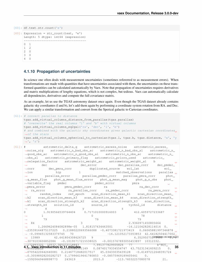
4.1.10 Propagation of uncertainties
In science one often deals with measurement uncertainties (sometimes refererred to as measurement errors). Whentransformations are made with quantities that have uncertainties associated with them, the uncertainties on these trans-formed quantities can be calculated automatically by Vaex. Note that propagation of uncertainties requires derivativesand matrix multiplications of lengthy equations, which is not complex, but tedious. Vaex can automatically calculateall dependencies, derivatives and compute the full covariance matrix.
As an example, let us use the TGAS astronomy dataset once again. Even though the TGAS dataset already containsgalactic sky coordiantes (l and b), let’s add them again by performing a coordinate system rotation from RA. and Dec.We can apply a similar transformation and convert from the Sperical galactic to Cartesian coordinates.
[61]: # convert parallas to distancetgas.add_virtual_columns_distance_from_parallax(tgas.parallax)# 'overwrite' the real columns 'l' and 'b' with virtual columnstgas.add_virtual_columns_eq2gal('ra', 'dec', 'l', 'b')# and combined with the galactic sky coordinates gives galactic cartesian coordinates→˓of the starstgas.add_virtual_columns_spherical_to_cartesian(tgas.l, tgas.b, tgas.distance, 'x', 'y→˓', 'z')
[61]: # astrometric_delta_q astrometric_excess_noise astrometric_excess_→˓noise_sig astrometric_n_bad_obs_ac astrometric_n_bad_obs_al astrometric_n_→˓good_obs_ac astrometric_n_good_obs_al astrometric_n_obs_ac astrometric_n_→˓obs_al astrometric_primary_flag astrometric_priors_used astrometric_→˓relegation_factor astrometric_weight_ac astrometric_weight_al b→˓ dec dec_error dec_parallax_corr dec_pmdec_→˓corr dec_pmra_corr duplicated_source ecl_lat ecl_→˓lon hip l matched_observations parallax→˓ parallax_error parallax_pmdec_corr parallax_pmra_corr phot_→˓g_mean_flux phot_g_mean_flux_error phot_g_mean_mag phot_g_n_obs phot_→˓variable_flag pmdec pmdec_error pmra→˓pmra_error pmra_pmdec_corr ra ra_dec_corr→˓ ra_error ra_parallax_corr ra_pmdec_corr ra_pmra_corr→˓ random_index ref_epoch scan_direction_mean_k1 scan_direction_mean_→˓k2 scan_direction_mean_k3 scan_direction_mean_k4 scan_direction_strength_→˓k1 scan_direction_strength_k2 scan_direction_strength_k3 scan_direction_→˓strength_k4 solution_id source_id tycho2_id distance→˓ x y z0 1.9190566539764404 0.7171010000916003 412.6059727233687→˓ 1 0 78→˓ 79 79 79→˓ 84 3 2.9360971450805664→˓ 1.2669624084082898e-05 1.818157434463501 -16.121042828114014 0.→˓23539164875137225 0.21880220693566088 -0.4073381721973419 0.06065881997346878→˓ -0.09945132583379745 70 -16.121052173353853 42.64182504417002→˓ 13989 42.641804308626725 9 6.35295075173405 0.→˓3079103606852086 -0.10195717215538025 -0.0015767893055453897 10312332.→˓172993332 10577.365273118843 7.991377829505826 77 b'NOT_→˓AVAILABLE' -7.641989988351149 0.08740179334554747 43.75231341609215 0.→˓07054220642640081 0.21467718482017517 45.03433035439128 -0.41497212648391724→˓0.30598928200282727 0.17996619641780853 -0.08575969189405441 0.→˓15920649468898773 243619 2015.0 -113.76032257080078 21.→˓39291763305664 -41.67839813232422 26.201841354370117 0.→˓3823484778404236 0.5382660627365112 0.3923785090446472→˓ 0.9163063168525696 1635378410781933568 7627862074752 b''→˓ 0.15740717016058217 0.11123604040005637 0.10243667003803988 -0.→˓04370685490397632
(continues on next page)
4.1. Vaex introduction in 11 minutes 35

vaex Documentation, Release 3.0.0-dev
(continued from previous page)
1 nan 0.2534628812968044 47.316290890180255→˓ 2 0 55→˓ 57 57 57→˓ 84 5 2.6523141860961914→˓ 3.1600175134371966e-05 12.861557006835938 -16.19302376369384 0.→˓2000676896877873 1.1977893944215496 0.8376259803771973 -0.9756439924240112→˓ 0.9725773334503174 70 -16.19303311057312 42.→˓761180489478576 -2147483648 42.76115974936648 8 3.→˓90032893506844 0.3234880030045522 -0.8537789583206177 0.8397389650344849→˓ 949564.6488279914 1140.173576223928 10.580958718900256 62→˓b'NOT_AVAILABLE' -55.10917285969142 2.522928801165149 10.03626300124532→˓ 4.611413518289133 -0.9963987469673157 45.1650067708984 -0.9959233403205872→˓ 2.583882288511597 -0.8609106540679932 0.9734798669815063 -0.→˓9724165201187134 487238 2015.0 -156.432861328125 22.→˓76607322692871 -36.23965835571289 22.890602111816406 0.→˓7110026478767395 0.9659702777862549 0.6461148858070374→˓ 0.8671600818634033 1635378410781933568 9277129363072 b'55-28-→˓1' 0.25638863199686845 0.1807701962996959 0.16716755815017084 -0.→˓071500169573954912 nan 0.3989006354041912 221.18496561724646→˓ 4 1 57→˓ 60 61 61→˓ 84 5 3.9934017658233643→˓ 2.5633918994572014e-05 5.767529487609863 -16.12335382439265 0.→˓24882543945301736 0.1803264123376257 -0.39189115166664124 -0.19325552880764008→˓ 0.08942046016454697 70 -16.123363170402296 42.69750168007008→˓ -2147483648 42.69748094193635 7 3.1553132200367373 0.→˓2734838183180671 -0.11855248361825943 -0.0418587327003479 817837.6000768564→˓ 1827.3836759985832 10.743102380434273 60 b'NOT_AVAILABLE'→˓ -1.602867102186794 1.0352589283446592 2.9322836829569003 1.908644426623371→˓ -0.9142706990242004 45.08615483797584 -0.1774432212114334 0.→˓2138361631952843 0.30772241950035095 -0.1848166137933731 0.04686680808663368→˓ 1948952 2015.0 -117.00751495361328 19.772153854370117→˓-43.108219146728516 26.7157039642334 0.4825277626514435 0.→˓4287584722042084 0.5241528153419495 0.9030616879463196→˓ 1635378410781933568 13297218905216 b'55-1191-1' 0.31692574722846595→˓0.22376103019475546 0.2064625216744117 -0.088012259182152053 nan 0.4224923646481251 179.98201436339852→˓ 1 0 51→˓ 52 52 52→˓ 84 5 4.215157985687256→˓ 2.8672602638835087e-05 5.3608622550964355 -16.118206879297034 0.→˓24821079122833972 0.20095844850181172 -0.33721715211868286 -0.22350119054317474→˓ 0.13181143999099731 70 -16.11821622503516 42.67779093546686→˓ -2147483648 42.67777019818556 7 2.292366835156796 0.→˓2809724206784257 -0.10920235514640808 -0.049440864473581314 602053.4754362862→˓ 905.8772856344845 11.075682394435745 61 b'NOT_AVAILABLE'→˓ -18.414912114825732 1.1298513589995536 3.661982345981763 2.065051873379775→˓ -0.9261773228645325 45.06654155758114 -0.36570677161216736 0.→˓2760390513575931 0.2028782218694687 -0.058928851038217545 -0.→˓050908856093883514 102321 2015.0 -132.42112731933594 22.→˓56928253173828 -38.95445251464844 25.878559112548828 0.→˓4946548640727997 0.6384561061859131 0.5090736746788025→˓ 0.8989177942276001 1635378410781933568 13469017597184 b'55-→˓624-1' 0.43623035574565916 0.30810014040531863 0.2840853806346911 -0.→˓121106247839861614 nan 0.3175001122010629 119.74837853832186→˓ 2 3 85→˓ 84 87 87→˓ 84 5 3.2356362342834473→˓ 2.22787512029754e-05 8.080779075622559 -16.055471830750374 0.→˓33504360351532875 0.1701298562030361 -0.43870800733566284 -0.27934885025024414→˓ 0.12179157137870789 70 -16.0554811777948 42.77336987816832→˓ -2147483648 42.77334913546197 11 1.582076960273368 0.→˓2615394689640736 -0.329196035861969 0.10031197965145111 1388122.242048847→˓ 2826.428866453177 10.168700781271088 96 b'NOT_AVAILABLE'→˓ -2.379387386351838 0.7106320061478508 0.34080233369502516 1.2204755227890713→˓ -0.8336043357849121 45.13603822322069 -0.049052558839321136 0.→˓17069695283376776 0.4714251756668091 -0.1563923954963684 -0.→˓15207625925540924 409284 2015.0 -106.85968017578125 4.→˓452099323272705 -47.8953971862793 26.755468368530273 0.→˓5206537842750549 0.23930974304676056 0.653376579284668→˓ 0.8633849024772644 1635378410781933568 15736760328576 b'55-→˓849-1' 0.6320805024726543 0.44587838095402044 0.41250283253756015 -0.→˓17481316927621393
(continues on next page)
36 Chapter 4. Tutorials

vaex Documentation, Release 3.0.0-dev
(continued from previous page)
... ... ... ...→˓ ... ... ...→˓ ... ... ...→˓ ... ... ...→˓ ... ... ... ...→˓ ... ... ... ...→˓ ... ... ...→˓... ... ... ... ...→˓ ... ... ...→˓... ... ... ...→˓... ... ... ...→˓... ... ... ...→˓ ... ... ... ...→˓ ... ... ... ...→˓ ... ... ...→˓ ... ... ...→˓ ... ... ... ...→˓ ... ...2,057,045 25.898868560791016 0.6508009723190962 172.3136755413185→˓ 0 0 54→˓ 54 54 54→˓ 84 3 6.386378765106201→˓ 1.8042501324089244e-05 2.2653496265411377 16.006806970347426 -0.→˓42319686025158043 0.24974147639642075 0.00821441039443016 0.2133195698261261→˓-0.000805279181804508 70 16.006807041815204 317.0782357688112→˓ 103561 -42.92178788756781 8 5.0743069397419776 0.→˓2840892420661878 -0.0308084636926651 -0.03397708386182785 4114975.455725508→˓ 3447.5776608146016 8.988851940956916 69 b'NOT_AVAILABLE'→˓ -4.440524133201202 0.04743297901782237 21.970772995655643 0.→˓07846893118669047 0.3920176327228546 314.74170043792924 0.08548042178153992→˓0.2773321068969684 0.2473779171705246 -0.0006040430744178593 0.→˓11652233451604843 1595738 2015.0 -18.078920364379883 -17.→˓731922149658203 38.27400588989258 27.63787269592285 0.→˓29217642545700073 0.11402469873428345 0.0404343381524086→˓ 0.937016487121582 1635378410781933568 6917488998546378368 b''→˓ 0.19707124773395138 0.13871698568448773 -0.12900211309069443 0.→˓0543427031363157842,057,046 nan 0.17407523451856974 28.886549102578012→˓ 0 2 54→˓ 52 54 54→˓ 84 5 1.9612410068511963→˓ 2.415467497485224e-05 24.774322509765625 16.12926993546893 -0.→˓32497534368232894 0.14823365569199975 0.8842677474021912 -0.9121489524841309→˓-0.8994856476783752 70 16.129270018016896 317.0105462544942→˓ -2147483648 -42.98947742356782 7 1.6983480817439922 0.→˓7410137777358506 -0.9793509840965271 -0.9959075450897217 1202425.→˓5197785893 871.2480333575235 10.324624601435723 59 b'NOT_→˓AVAILABLE' -10.401225111268962 1.4016954983272711 -1.2835612990841874 2.→˓7416807292293637 0.980453610420227 314.64381789311193 0.8981446623802185→˓0.3590974400544809 0.9818224906921387 -0.9802247881889343 -0.→˓9827051162719727 2019553 2015.0 -87.07184600830078 -31.→˓574886322021484 -36.37055206298828 29.130958557128906 0.→˓22651544213294983 0.07730517536401749 0.2675701975822449→˓ 0.9523505568504333 1635378410781933568 6917493705830041600 b'5179-→˓753-1' 0.5888074481016426 0.4137467499267554 -0.38568304807850484 0.→˓163573910786192462,057,047 nan 0.47235246463190794 92.12190417660749→˓ 2 0 34→˓ 36 36 36→˓ 84 5 4.68601131439209→˓ 2.138371200999245e-05 3.9279115200042725 15.92496896432183 -0.→˓34317732044320387 0.20902981533215972 -0.2000708132982254 0.31042322516441345→˓-0.3574342727661133 70 15.924968943694909 317.6408327998631→˓ -2147483648 -42.359190842094414 6 6.036938108863445 0.→˓39688014089787665 -0.7275367975234985 -0.25934046506881714 3268640.→˓5253614695 4918.5087736624755 9.238852161621992 51 b'NOT_→˓AVAILABLE' -27.852344752672245 1.2778575351686428 15.713555906870294 0.→˓9411842746983148 -0.1186852976679802 315.2828795933192 -0.47665935754776→˓0.4722647631556871 0.704002320766449 -0.77033931016922 0.→˓12704335153102875 788948 2015.0 -21.23501205444336 20.→˓132535934448242 33.55913162231445 26.732301712036133 0.→˓41511622071266174 0.5105549693107605 0.15976844727993011→˓ 0.9333845376968384 1635378410781933568 6917504975824469248 b'5192-→˓877-1' 0.16564688621402263 0.11770477437507047 -0.10732559074953243 0.→˓045449912782963474
(continues on next page)
4.1. Vaex introduction in 11 minutes 37

vaex Documentation, Release 3.0.0-dev
(continued from previous page)
2,057,048 nan 0.3086465263182493 76.66564461310193→˓ 1 2 52→˓ 51 53 53→˓ 84 5 3.154139280319214→˓ 1.9043474821955897e-05 9.627826690673828 16.193728871838935 -0.→˓22811360043544882 0.131650037775767 0.3082593083381653 -0.5279345512390137→˓-0.4065483510494232 70 16.193728933791913 317.1363617703344→˓ -2147483648 -42.86366191921117 7 1.484142306295484 0.→˓34860128377301614 -0.7272516489028931 -0.9375584125518799 4009408.→˓3172682906 1929.9834553649182 9.017069346445364 60 b'NOT_→˓AVAILABLE' 1.8471079057572073 0.7307171627866237 11.352888915160555 1.→˓219847308406543 0.7511345148086548 314.7406481637209 0.41397571563720703→˓0.19205296641778563 0.7539510726928711 -0.7239754796028137 -0.→˓7911394238471985 868066 2015.0 -89.73970794677734 -25.→˓196216583251953 -35.13546371459961 29.041872024536133 0.→˓21430812776088715 0.06784655898809433 0.2636755108833313→˓ 0.9523414969444275 1635378410781933568 6917517998165066624 b'5179-→˓1401-1' 0.6737898352187435 0.4742760432178817 -0.44016428945980135 0.→˓187910550949220772,057,049 nan 0.4329850465924866 60.789771079095715→˓ 0 0 26→˓ 26 26 26→˓ 84 5 4.3140177726745605→˓ 2.7940122890868224e-05 4.742301940917969 16.135962442685898 -0.→˓22130081624351935 0.2686748166142929 -0.46605369448661804 0.30018869042396545→˓-0.3290684223175049 70 16.13596246842634 317.3575812619557→˓ -2147483648 -42.642442417388324 5 2.680111343641743 0.→˓4507741964825321 -0.689416229724884 -0.1735922396183014 2074338.153903563→˓ 4136.498086035368 9.732571175024953 31 b'NOT_AVAILABLE'→˓ 3.15173423618292 1.4388911228835037 2.897878776243949 1.0354817855168323→˓ -0.21837876737117767 314.960730599014 -0.4467950165271759 0.→˓49182050944792216 0.7087226510047913 -0.8360105156898499 0.2156151533126831→˓ 1736132 2015.0 -63.01319885253906 18.303699493408203→˓-49.05630111694336 28.76698875427246 0.3929939866065979 0.→˓32352808117866516 0.24211134016513824 0.9409775733947754→˓ 1635378410781933568 6917521537218608640 b'5179-1719-1' 0.3731188267130712→˓0.2636519673685346 -0.24280110216486334 0.10369630532457579
Since RA. and Dec. are in degrees, while ra_error and dec_error are in miliarcseconds, we need put them on the samescale
[62]: tgas['ra_error'] = tgas.ra_error / 1000 / 3600tgas['dec_error'] = tgas.dec_error / 1000 / 3600
We now let Vaex sort out what the covariance matrix is for the Cartesian coordinates x, y, and z. Then take 50 samplesfrom the dataset for visualization.
[63]: tgas.propagate_uncertainties([tgas.x, tgas.y, tgas.z])tgas_50 = tgas.sample(50, random_state=42)
For this small subset of the dataset we can visualize the uncertainties, with and without the covariance.
[64]: tgas_50.scatter(tgas_50.x, tgas_50.y, xerr=tgas_50.x_uncertainty, yerr=tgas_50.y_→˓uncertainty)plt.xlim(-10, 10)plt.ylim(-10, 10)
(continues on next page)
38 Chapter 4. Tutorials

vaex Documentation, Release 3.0.0-dev
(continued from previous page)
plt.show()tgas_50.scatter(tgas_50.x, tgas_50.y, xerr=tgas_50.x_uncertainty, yerr=tgas_50.y_→˓uncertainty, cov=tgas_50.y_x_covariance)plt.xlim(-10, 10)plt.ylim(-10, 10)plt.show()
From the second plot, we see that showing error ellipses (so narrow that they appear as lines) instead of error barsreveal that the distance information dominates the uncertainty in this case.
4.1.11 Just-In-Time compilation
Let us start with a function that calculates the angular distance between two points on a surface of a sphere. The inputof the function is a pair of 2 angular coordinates, in radians.
[65]: import vaeximport numpy as np
(continues on next page)
4.1. Vaex introduction in 11 minutes 39

vaex Documentation, Release 3.0.0-dev
(continued from previous page)
# From http://pythonhosted.org/pythran/MANUAL.htmldef arc_distance(theta_1, phi_1, theta_2, phi_2):
"""Calculates the pairwise arc distancebetween all points in vector a and b."""temp = (np.sin((theta_2-2-theta_1)/2)**2
+ np.cos(theta_1)*np.cos(theta_2) * np.sin((phi_2-phi_1)/2)**2)distance_matrix = 2 * np.arctan2(np.sqrt(temp), np.sqrt(1-temp))return distance_matrix
Let us use the New York Taxi dataset of 2015, as can be downloaded in hdf5 format
[66]: # nytaxi = vaex.open('s3://vaex/taxi/yellow_taxi_2009_2015_f32.hdf5?anon=true')nytaxi = vaex.open('/Users/jovan/Work/vaex-work/vaex-taxi/data/yellow_taxi_2009_2015_→˓f32.hdf5')# lets use just 20% of the data, since we want to make sure it fits# into memory (so we don't measure just hdd/ssd speed)nytaxi.set_active_fraction(0.2)
Although the function above expects Numpy arrays, Vaex can pass in columns or expression, which will delay theexecution untill it is needed, and add the resulting expression as a virtual column.
[67]: nytaxi['arc_distance'] = arc_distance(nytaxi.pickup_longitude * np.pi/180,nytaxi.pickup_latitude * np.pi/180,nytaxi.dropoff_longitude * np.pi/180,nytaxi.dropoff_latitude * np.pi/180)
When we calculate the mean angular distance of a taxi trip, we encounter some invalid data, that will give warnings,which we can safely ignore for this demonstration.
[68]: %%timenytaxi.mean(nytaxi.arc_distance)
/Users/jovan/PyLibrary/vaex/packages/vaex-core/vaex/functions.py:121: RuntimeWarning:→˓invalid value encountered in sqrtreturn function(*args, **kwargs)
/Users/jovan/PyLibrary/vaex/packages/vaex-core/vaex/functions.py:121: RuntimeWarning:→˓invalid value encountered in sinreturn function(*args, **kwargs)
/Users/jovan/PyLibrary/vaex/packages/vaex-core/vaex/functions.py:121: RuntimeWarning:→˓invalid value encountered in cosreturn function(*args, **kwargs)
CPU times: user 44.5 s, sys: 5.03 s, total: 49.5 sWall time: 6.14 s
[68]: array(1.99993285)
This computation uses quite some heavy mathematical operations, and since it’s (internally) using Numpy arrays,also uses quite some temporary arrays. We can optimize this calculation by doing a Just-In-Time compilation, basedon numba, pythran, or if you happen to have an NVIDIA graphics card cuda. Choose whichever gives the bestperformance or is easiest to install.
[69]: nytaxi['arc_distance_jit'] = nytaxi.arc_distance.jit_numba()# nytaxi['arc_distance_jit'] = nytaxi.arc_distance.jit_pythran()# nytaxi['arc_distance_jit'] = nytaxi.arc_distance.jit_cuda()
40 Chapter 4. Tutorials

vaex Documentation, Release 3.0.0-dev
[70]: %%timenytaxi.mean(nytaxi.arc_distance_jit)
/Users/jovan/PyLibrary/vaex/packages/vaex-core/vaex/expression.py:1038:→˓RuntimeWarning: invalid value encountered in freturn self.f(*args, **kwargs)
CPU times: user 25.7 s, sys: 330 ms, total: 26 sWall time: 2.31 s
[70]: array(1.9999328)
We can get a significant speedup (∼ 3𝑥) in this case.
4.1.12 Parallel computations
As mentioned in the sections on selections, Vaex can do computations in parallel. Often this is taken care of, forinstance, when passing multiple selections to a method, or multiple arguments to one of the statistical functions.However, sometimes it is difficult or impossible to express a computation in one expression, and we need to resort todoing so called ‘delayed’ computation, similar as in joblib and dask.
[71]: import vaexdf = vaex.example()limits = [-10, 10]delayed_count = df.count(df.E, binby=df.x, limits=limits,
shape=4, delay=True)delayed_count
[71]: <vaex.promise.Promise at 0x7ffbd64072d0>
Note that now the returned value is now a promise (TODO: a more Pythonic way would be to return a Future). This maybe subject to change, and the best way to work with this is to use the delayed decorator. And call DataFrame.executewhen the result is needed.
In addition to the above delayed computation, we schedule more computation, such that both the count and mean areexecuted in parallel such that we only do a single pass over the data. We schedule the execution of two extra functionsusing the vaex.delayed decorator, and run the whole pipeline using df.execute().
[72]: delayed_sum = df.sum(df.E, binby=df.x, limits=limits,shape=4, delay=True)
@vaex.delayeddef calculate_mean(sums, counts):
print('calculating mean')return sums/counts
print('before calling mean')# since calculate_mean is decorated with vaex.delayed# this now also returns a 'delayed' object (a promise)delayed_mean = calculate_mean(delayed_sum, delayed_count)
# if we'd like to perform operations on that, we can again# use the same [email protected] print_mean(means):
print('means', means)print_mean(delayed_mean)
(continues on next page)
4.1. Vaex introduction in 11 minutes 41

vaex Documentation, Release 3.0.0-dev
(continued from previous page)
print('before calling execute')df.execute()
# Using the .get on the promise will also return the result# However, this will only work after execute, and may be# subject to changemeans = delayed_mean.get()print('same means', means)
before calling meanbefore calling executecalculating meanmeans [ -94323.68051598 -118749.23850834 -119119.46292653 -95021.66183457]same means [ -94323.68051598 -118749.23850834 -119119.46292653 -95021.66183457]
4.1.13 Extending Vaex
Vaex can be extended using several mechanisms.
Adding functions
Use the vaex.register_function decorator API to add new functions.
[73]: import vaeximport numpy as [email protected]_function()def add_one(ar):
return ar+1
The function can be invoked using the df.func accessor, to return a new expression. Each argument that is anexpresssion, will be replaced by a Numpy array on evaluations in any Vaex context.
[74]: df = vaex.from_arrays(x=np.arange(4))df.func.add_one(df.x)
[74]: Expression = add_one(x)Length: 4 dtype: int64 (expression)-----------------------------------0 11 22 33 4
By default (passing on_expression=True), the function is also available as a method on Expressions, where theexpression itself is automatically set as the first argument (since this is a quite common use case).
[75]: df.x.add_one()
[75]: Expression = add_one(x)Length: 4 dtype: int64 (expression)-----------------------------------0 11 2
(continues on next page)
42 Chapter 4. Tutorials

vaex Documentation, Release 3.0.0-dev
(continued from previous page)
2 33 4
In case the first argument is not an expression, pass on_expression=True, and use df.func.<funcname>,to build a new expression using the function:
[76]: @vaex.register_function(on_expression=False)def addmul(a, b, x, y):
return a*x + b * y
[77]: df = vaex.from_arrays(x=np.arange(4))df['y'] = df.x**2df.func.addmul(2, 3, df.x, df.y)
[77]: Expression = addmul(2, 3, x, y)Length: 4 dtype: int64 (expression)-----------------------------------0 01 52 163 33
These expressions can be added as virtual columns, as expected.
[78]: df = vaex.from_arrays(x=np.arange(4))df['y'] = df.x**2df['z'] = df.func.addmul(2, 3, df.x, df.y)df['w'] = df.x.add_one()df
[78]: # x y z w0 0 0 0 11 1 1 5 22 2 4 16 33 3 9 33 4
Adding DataFrame accessors
When adding methods that operate on Dataframes, it makes sense to group them together in a single namespace.
[79]: @vaex.register_dataframe_accessor('scale', override=True)class ScalingOps(object):
def __init__(self, df):self.df = df
def mul(self, a):df = self.df.copy()for col in df.get_column_names(strings=False):
if df[col].dtype:df[col] = df[col] * a
return df
def add(self, a):df = self.df.copy()for col in df.get_column_names(strings=False):
(continues on next page)
4.1. Vaex introduction in 11 minutes 43

vaex Documentation, Release 3.0.0-dev
(continued from previous page)
if df[col].dtype:df[col] = df[col] + a
return df
[80]: df.scale.add(1)
[80]: # x y z w0 1 1 1 21 2 2 6 32 3 5 17 43 4 10 34 5
[81]: df.scale.mul(2)
[81]: # x y z w0 0 0 0 21 2 2 10 42 4 8 32 63 6 18 66 8
<style> pre white-space: pre-wrap !important; .table-striped > tbody > tr:nth-of-type(odd) background-color: f9f9f9; .table-striped > tbody > tr:nth-of-type(even) background-color: white; .table-striped td,.table-striped th, .table-striped tr border: 1px solid black; border-collapse: collapse; margin: 1em 2em;.renderedℎ𝑡𝑚𝑙𝑡𝑑, .𝑟𝑒𝑛𝑑𝑒𝑟𝑒𝑑ℎ𝑡𝑚𝑙𝑡ℎ𝑡𝑒𝑥𝑡− 𝑎𝑙𝑖𝑔𝑛 : 𝑙𝑒𝑓𝑡; 𝑣𝑒𝑟𝑡𝑖𝑐𝑎𝑙 − 𝑎𝑙𝑖𝑔𝑛 : 𝑚𝑖𝑑𝑑𝑙𝑒; 𝑝𝑎𝑑𝑑𝑖𝑛𝑔 : 4𝑝𝑥; < /𝑠𝑡𝑦𝑙𝑒 >
4.2 Machine Learning with vaex.ml
The vaex.ml package brings some machine learning algorithms to vaex. If you installed the individual subpackages(vaex-core, vaex-hdf5, . . . ) instead of the vaex metapackage, you may need to install it by running pipinstall vaex-ml, or conda install -c conda-forge vaex-ml.
The API of vaex.ml stays close to that of scikit-learn, while providing better performance and the ability to ef-ficiently perform operations on data that is larger than the available RAM. This page is an overview and a briefintroduction to the capabilities offered by vaex.ml.
[1]: import vaeximport vaex.ml
import numpy as npimport pylab as plt
We will use the well known Iris flower and Titanic passenger list datasets, two classical datasets for machine learningdemonstrations.
[2]: df = vaex.ml.datasets.load_iris()df
[2]: # sepal_length sepal_width petal_length petal_width class_0 5.9 3.0 4.2 1.5 11 6.1 3.0 4.6 1.4 12 6.6 2.9 4.6 1.3 13 6.7 3.3 5.7 2.1 24 5.5 4.2 1.4 0.2 0... ... ... ... ... ...
(continues on next page)
44 Chapter 4. Tutorials

vaex Documentation, Release 3.0.0-dev
(continued from previous page)
145 5.2 3.4 1.4 0.2 0146 5.1 3.8 1.6 0.2 0147 5.8 2.6 4.0 1.2 1148 5.7 3.8 1.7 0.3 0149 6.2 2.9 4.3 1.3 1
[3]: df.scatter(df.petal_length, df.petal_width, c_expr=df.class_);
4.2.1 Preprocessing: Scaling of numerical features
vaex.ml packs the common numerical scalers:
• vaex.ml.StandardScaler - Scale features by removing their mean and dividing by their variance;
• vaex.ml.MinMaxScaler - Scale features to a given range;
• vaex.ml.RobustScaler - Scale features by removing their median and scaling them according to a givenpercentile range;
• vaex.ml.MaxAbsScaler - Scale features by their maximum absolute value.
The usage is quite similar to that of scikit-learn, in the sense that each transformer implements the .fit and.transform methods.
[4]: features = ['petal_length', 'petal_width', 'sepal_length', 'sepal_width']scaler = vaex.ml.StandardScaler(features=features, prefix='scaled_')scaler.fit(df)df_trans = scaler.transform(df)df_trans
[4]: # sepal_length sepal_width petal_length petal_width class_ scaled_→˓petal_length scaled_petal_width scaled_sepal_length scaled_sepal_width0 5.9 3.0 4.2 1.5 1 0.→˓25096730693923325 0.39617188299171285 0.06866179325140277 -0.→˓124957601171306071 6.1 3.0 4.6 1.4 1 0.→˓4784301228962429 0.26469891297233916 0.3109975341387059 -0.→˓12495760117130607
(continues on next page)
4.2. Machine Learning with vaex.ml 45

vaex Documentation, Release 3.0.0-dev
(continued from previous page)
2 6.6 2.9 4.6 1.3 1 0.→˓4784301228962429 0.13322594295296575 0.9168368863569659 -0.→˓35636056630335723 6.7 3.3 5.7 2.1 2 1.→˓1039528667780207 1.1850097031079545 1.0380047568006185 0.→˓56925129422484634 5.5 4.2 1.4 0.2 0 -1.→˓341272404759837 -1.3129767272601438 -0.4160096885232057 2.6518779804133055... ... ... ... ... ... ...→˓ ... ... ...145 5.2 3.4 1.4 0.2 0 -1.→˓341272404759837 -1.3129767272601438 -0.7795132998541615 0.8006542593568975146 5.1 3.8 1.6 0.2 0 -1.→˓2275409967813318 -1.3129767272601438 -0.9006811702978141 1.726266119885101147 5.8 2.6 4.0 1.2 1 0.→˓13723589896072813 0.0017529729335920385 -0.052506077192249874 -1.→˓0505694616995096148 5.7 3.8 1.7 0.3 0 -1.→˓1706752927920796 -1.18150375724077 -0.17367394763590144 1.726266119885101149 6.2 2.9 4.3 1.3 1 0.→˓30783301092848553 0.13322594295296575 0.4321654045823586 -0.→˓3563605663033572
The output of the .transform method of any vaex.ml transformer is a shallow copy of a DataFrame that containsthe resulting features of the transformations in addition to the original columns. A shallow copy means that this newDataFrame just references the original one, and no extra memory is used. In addition, the resulting features, in thiscase the scaled numerical features are virtual columns, which do not take any memory but are computed on the flywhen needed. This approach is ideal for working with very large datasets.
Preprocessing: Encoding of categorical features
vaex.ml contains several categorical encoders:
• vaex.ml.LabelEncoder - Encoding features with as many integers as categories, startinfg from 0;
• vaex.ml.OneHotEncoder - Encoding features according to the one-hot scheme;
• vaex.ml.FrequencyEncoder - Encode features by the frequency of their respective categories;
• vaex.ml.BayesianTargetEncoder - Encode categories with the mean of their target value;
• vaex.ml.WeightOfEvidenceEncoder - Encode categories their weight of evidence value.
The following is a quick example using the Titanic dataset.
[5]: df = vaex.ml.datasets.load_titanic()df.head(5)
[5]: # pclass survived name sex→˓ age sibsp parch ticket fare cabin embarked boat body→˓home_dest0 1 True Allen, Miss. Elisabeth Walton female
→˓29 0 0 24160 211.338 B5 S 2 nan→˓St Louis, MO1 1 True Allison, Master. Hudson Trevor male
→˓0.9167 1 2 113781 151.55 C22 C26 S 11 nan→˓Montreal, PQ / Chesterville, ON2 1 False Allison, Miss. Helen Loraine female
→˓2 1 2 113781 151.55 C22 C26 S None nan→˓Montreal, PQ / Chesterville, ON
(continues on next page)
46 Chapter 4. Tutorials

vaex Documentation, Release 3.0.0-dev
(continued from previous page)
3 1 False Allison, Mr. Hudson Joshua Creighton male→˓30 1 2 113781 151.55 C22 C26 S None 135→˓Montreal, PQ / Chesterville, ON4 1 False Allison, Mrs. Hudson J C (Bessie Waldo Daniels) female
→˓25 1 2 113781 151.55 C22 C26 S None nan→˓Montreal, PQ / Chesterville, ON
[6]: label_encoder = vaex.ml.LabelEncoder(features=['embarked'])one_hot_encoder = vaex.ml.OneHotEncoder(features=['pclass'])freq_encoder = vaex.ml.FrequencyEncoder(features=['home_dest'])
df = label_encoder.fit_transform(df)df = one_hot_encoder.fit_transform(df)df = freq_encoder.fit_transform(df)
df.head(5)
[6]: # pclass survived name sex→˓ age sibsp parch ticket fare cabin embarked boat body→˓home_dest label_encoded_embarked pclass_1 pclass_2→˓ pclass_3 frequency_encoded_home_dest0 1 True Allen, Miss. Elisabeth Walton female
→˓29 0 0 24160 211.338 B5 S 2 nan→˓St Louis, MO 1 1 0→˓ 0 0.003055771 1 True Allison, Master. Hudson Trevor male
→˓0.9167 1 2 113781 151.55 C22 C26 S 11 nan→˓Montreal, PQ / Chesterville, ON 1 1 0→˓ 0 0.003055772 1 False Allison, Miss. Helen Loraine female
→˓2 1 2 113781 151.55 C22 C26 S None nan→˓Montreal, PQ / Chesterville, ON 1 1 0→˓ 0 0.003055773 1 False Allison, Mr. Hudson Joshua Creighton male
→˓30 1 2 113781 151.55 C22 C26 S None 135→˓Montreal, PQ / Chesterville, ON 1 1 0→˓ 0 0.003055774 1 False Allison, Mrs. Hudson J C (Bessie Waldo Daniels) female
→˓25 1 2 113781 151.55 C22 C26 S None nan→˓Montreal, PQ / Chesterville, ON 1 1 0→˓ 0 0.00305577
Notice that the transformed features are all included in the resulting DataFrame and are appropriately named. This isexcellent for the construction of various diagnostic plots, and engineering of more complex features. The fact that theresulting (encoded) features take no memory, allows one to try out or combine a variety of preprocessing steps withoutspending any extra memory.
4.2.2 Dimensionality reduction
Principal Component Analysis
The PCA implemented in vaex.ml can scale to a very large number of samples, even if that data we want to transformdoes not fit into RAM. To demonstrate this, let us do a PCA transformation on the Iris dataset. For this example, wehave replicated this dataset thousands of times, such that it contains over 1 billion samples.
4.2. Machine Learning with vaex.ml 47

vaex Documentation, Release 3.0.0-dev
[7]: df = vaex.ml.datasets.load_iris_1e9()n_samples = len(df)print(f'Number of samples in DataFrame: {n_samples:,}')
Number of samples in DataFrame: 1,005,000,000
[8]: features = ['petal_length', 'petal_width', 'sepal_length', 'sepal_width']pca = vaex.ml.PCA(features=features, n_components=4, progress=True)pca.fit(df)
[########################################] 100.00% elapsed time : 25.39s = 0.4m→˓= 0.0h[########################################] 100.00% elapsed time : 21.16s = 0.4m→˓= 0.0h
The PCA transformer implemented in vaex.ml can be fit in well under a minute, even when the data comprises 4columns and 1 billion rows.
[9]: df_trans = pca.transform(df)df_trans
[9]: # sepal_length sepal_width petal_length petal_width class_→˓ PCA_0 PCA_1 PCA_2 PCA_30 5.9 3.0 4.2 1.5 1→˓ -0.5110980606779778 0.10228410712350186 0.1323278893222748 -0.→˓050100535092195681 6.1 3.0 4.6 1.4 1→˓ -0.8901604458458314 0.03381244392899576 -0.009768027251340669 0.→˓153448205958539722 6.6 2.9 4.6 1.3 1→˓ -1.0432977815146882 -0.22895691422385436 -0.4148145621997159 0.→˓037523552124690923 6.7 3.3 5.7 2.1 2→˓ -2.275853649499827 -0.33338651939283853 0.28467815929803336 0.→˓0622302805873101864 5.5 4.2 1.4 0.2 0→˓ 2.5971594761444177 -1.1000219272349778 0.1635819259153647 0.→˓09895807663018358... ... ... ... ... ...→˓ ... ... ... ...1,004,999,995 5.2 3.4 1.4 0.2 0→˓ 2.639821267772449 -0.31929007064114523 -0.13925337154239886 -0.→˓065141046610320821,004,999,996 5.1 3.8 1.6 0.2 0→˓ 2.537573370562511 -0.5103675440827672 0.17191840827679977 0.→˓192165949220465451,004,999,997 5.8 2.6 4.0 1.2 1→˓ -0.2288790500828927 0.402257616677128 -0.22736271123587368 -0.→˓0186204541690075661,004,999,998 5.7 3.8 1.7 0.3 0→˓ 2.199077960400875 -0.8792440918495404 -0.1145214537809282 -0.→˓0253269362528850961,004,999,999 6.2 2.9 4.3 1.3 1→˓ -0.6416902785957136 -0.019071179119340448 -0.20417287643043353 0.→˓02050967499165212
Recall that the transformed DataFrame, which includes the PCA components, takes no extra memory.
48 Chapter 4. Tutorials

vaex Documentation, Release 3.0.0-dev
4.2.3 Clustering
K-Means
vaex.ml implements a fast and scalable K-Means clustering algorithm. The usage is similar to that ofscikit-learn.
[10]: import vaex.ml.cluster
df = vaex.ml.datasets.load_iris()
features = ['petal_length', 'petal_width', 'sepal_length', 'sepal_width']kmeans = vaex.ml.cluster.KMeans(features=features, n_clusters=3, max_iter=100,→˓verbose=True, random_state=42)kmeans.fit(df)
df_trans = kmeans.transform(df)df_trans
Iteration 0, inertia 519.0500000000001Iteration 1, inertia 156.70447116074328Iteration 2, inertia 88.70688235734133Iteration 3, inertia 80.23054939305554Iteration 4, inertia 79.28654263977778Iteration 5, inertia 78.94084142614601Iteration 6, inertia 78.94084142614601
[10]: # sepal_length sepal_width petal_length petal_width class_→˓prediction_kmeans0 5.9 3.0 4.2 1.5 1 01 6.1 3.0 4.6 1.4 1 02 6.6 2.9 4.6 1.3 1 03 6.7 3.3 5.7 2.1 2 14 5.5 4.2 1.4 0.2 0 2... ... ... ... ... ... ...145 5.2 3.4 1.4 0.2 0 2146 5.1 3.8 1.6 0.2 0 2147 5.8 2.6 4.0 1.2 1 0148 5.7 3.8 1.7 0.3 0 2149 6.2 2.9 4.3 1.3 1 0
K-Means is an unsupervised algorithm, meaning that the predicted cluster labels in the transformed dataset do notnecessarily correspond to the class label. We can map the predicted cluster identifiers to match the class labels,making it easier to construct diagnostic plots.
[11]: df_trans['predicted_kmean_map'] = df_trans.prediction_kmeans.map(mapper={0: 1, 1: 2,→˓2: 0})df_trans
[11]: # sepal_length sepal_width petal_length petal_width class_→˓prediction_kmeans predicted_kmean_map0 5.9 3.0 4.2 1.5 1 0→˓ 11 6.1 3.0 4.6 1.4 1 0→˓ 12 6.6 2.9 4.6 1.3 1 0→˓ 13 6.7 3.3 5.7 2.1 2 1→˓ 2
(continues on next page)
4.2. Machine Learning with vaex.ml 49

vaex Documentation, Release 3.0.0-dev
(continued from previous page)
4 5.5 4.2 1.4 0.2 0 2→˓ 0... ... ... ... ... ... ...→˓ ...145 5.2 3.4 1.4 0.2 0 2→˓ 0146 5.1 3.8 1.6 0.2 0 2→˓ 0147 5.8 2.6 4.0 1.2 1 0→˓ 1148 5.7 3.8 1.7 0.3 0 2→˓ 0149 6.2 2.9 4.3 1.3 1 0→˓ 1
Now we can construct simple scatter plots, and see that in the case of the Iris dataset, K-Means does a pretty good jobsplitting the data into 3 classes.
[12]: fig = plt.figure(figsize=(12, 5))
plt.subplot(121)df_trans.scatter(df_trans.petal_length, df_trans.petal_width, c_expr=df_trans.class_)plt.title('Original classes')
plt.subplot(122)df_trans.scatter(df_trans.petal_length, df_trans.petal_width, c_expr=df_trans.→˓predicted_kmean_map)plt.title('Predicted classes')
plt.tight_layout()plt.show()
As with any algorithm implemented in vaex.ml, K-Means can be used on billions of samples. Fitting takes under 2minutes when applied on the oversampled Iris dataset, numbering over 1 billion samples.
[13]: df = vaex.ml.datasets.load_iris_1e9()n_samples = len(df)print(f'Number of samples in DataFrame: {n_samples:,}')
50 Chapter 4. Tutorials

vaex Documentation, Release 3.0.0-dev
Number of samples in DataFrame: 1,005,000,000
[14]: %%time
features = ['petal_length', 'petal_width', 'sepal_length', 'sepal_width']kmeans = vaex.ml.cluster.KMeans(features=features, n_clusters=3, max_iter=100,→˓verbose=True, random_state=31)kmeans.fit(df)
Iteration 0, inertia 838974000.003719Iteration 1, inertia 535903134.00030565Iteration 2, inertia 530190921.4848897Iteration 3, inertia 528931941.0337245Iteration 4, inertia 528931941.03372455CPU times: user 4min 7s, sys: 1min 33s, total: 5min 41sWall time: 1min 23s
4.2.4 Supervised learning
While vaex.ml does not yet implement any supervised machine learning models, it does provide wrappers to severalpopular libraries such as scikit-learn, XGBoost, LightGBM and CatBoost.
The main benefit of these wrappers is that they turn the models into vaex.ml transformers. This means the modelsbecome part of the DataFrame state and thus can be serialized, and their predictions can be returned as virtual columns.This is especially useful for creating various diagnostic plots and evaluating performance metrics at no memory cost,as well as building ensembles.
Scikit-Learn example
The vaex.ml.sklearn module provides convenient wrappers to the scikit-learn estimators. In fact, thesewrappers can be used with any library that follows the API convention established by scikit-learn, i.e. imple-ments the .fit and .transform methods.
Here is an example:
[15]: from vaex.ml.sklearn import Predictorfrom sklearn.ensemble import GradientBoostingClassifier
df = vaex.ml.datasets.load_iris()
features = ['petal_length', 'petal_width', 'sepal_length', 'sepal_width']target = 'class_'
model = GradientBoostingClassifier(random_state=42)vaex_model = Predictor(features=features, target=target, model=model, prediction_name=→˓'prediction')
vaex_model.fit(df=df)
df = vaex_model.transform(df)df
[15]: # sepal_length sepal_width petal_length petal_width class_→˓prediction0 5.9 3.0 4.2 1.5 1 1
(continues on next page)
4.2. Machine Learning with vaex.ml 51

vaex Documentation, Release 3.0.0-dev
(continued from previous page)
1 6.1 3.0 4.6 1.4 1 12 6.6 2.9 4.6 1.3 1 13 6.7 3.3 5.7 2.1 2 24 5.5 4.2 1.4 0.2 0 0... ... ... ... ... ... ...145 5.2 3.4 1.4 0.2 0 0146 5.1 3.8 1.6 0.2 0 0147 5.8 2.6 4.0 1.2 1 1148 5.7 3.8 1.7 0.3 0 0149 6.2 2.9 4.3 1.3 1 1
One can still train a predictive model on datasets that are too big to fit into memory by leveraging the on-line learnersprovided by scikit-learn. The vaex.ml.sklearn.IncrementalPredictor conveniently wraps theselearners and provides control on how the data is passed to them from a vaex DataFrame.
Let us train a model on the oversampled Iris dataset which comprises over 1 billion samples.
[16]: from vaex.ml.sklearn import IncrementalPredictorfrom sklearn.linear_model import SGDClassifier
df = vaex.ml.datasets.load_iris_1e9()
features = ['petal_length', 'petal_width', 'sepal_length', 'sepal_width']target = 'class_'
model = SGDClassifier(learning_rate='constant', eta0=0.0001, random_state=42)vaex_model = IncrementalPredictor(features=features, target=target, model=model,
batch_size=11_000_000, partial_fit_kwargs={'classes→˓':[0, 1, 2]})
vaex_model.fit(df=df, progress=True)
df = vaex_model.transform(df)df
[########################################] 100.00% elapsed time : 747.59s = 12.5m→˓= 0.2h
[16]: # sepal_length sepal_width petal_length petal_width class_→˓ prediction0 5.9 3.0 4.2 1.5 1→˓ 11 6.1 3.0 4.6 1.4 1→˓ 12 6.6 2.9 4.6 1.3 1→˓ 13 6.7 3.3 5.7 2.1 2→˓ 24 5.5 4.2 1.4 0.2 0→˓ 0... ... ... ... ... ...→˓ ...1,004,999,995 5.2 3.4 1.4 0.2 0→˓ 01,004,999,996 5.1 3.8 1.6 0.2 0→˓ 01,004,999,997 5.8 2.6 4.0 1.2 1→˓ 1 (continues on next page)
52 Chapter 4. Tutorials

vaex Documentation, Release 3.0.0-dev
(continued from previous page)
1,004,999,998 5.7 3.8 1.7 0.3 0→˓ 01,004,999,999 6.2 2.9 4.3 1.3 1→˓ 1
XGBoost example
Libraries such as XGBoost provide more options such as validation during training and early stopping for example.We provide wrappers that keeps close to the native API of these libraries, in addition to the scikit-learn API.
While the following example showcases the XGBoost wrapper, vaex.ml implements similar wrappers forLightGBM and CatBoost.
[17]: from vaex.ml.xgboost import XGBoostModel
df = vaex.ml.datasets.load_iris_1e5()df_train, df_test = df.ml.train_test_split(test_size=0.2, verbose=False)
features = ['petal_length', 'petal_width', 'sepal_length', 'sepal_width']target = 'class_'
params = {'learning_rate': 0.1,'max_depth': 3,'num_class': 3,'objective': 'multi:softmax','subsample': 1,'random_state': 42,'n_jobs': -1}
booster = XGBoostModel(features=features, target=target, num_boost_round=500,→˓params=params)booster.fit(df=df_train, evals=[(df_train, 'train'), (df_test, 'test')], early_→˓stopping_rounds=5)
df_test = booster.transform(df_train)df_test
[17]: # sepal_length sepal_width petal_length petal_width class_→˓xgboost_prediction0 5.9 3.0 4.2 1.5 1 1.01 6.1 3.0 4.6 1.4 1 1.02 6.6 2.9 4.6 1.3 1 1.03 6.7 3.3 5.7 2.1 2 2.04 5.5 4.2 1.4 0.2 0 0.0... ... ... ... ... ... ...80,395 5.2 3.4 1.4 0.2 0 0.080,396 5.1 3.8 1.6 0.2 0 0.080,397 5.8 2.6 4.0 1.2 1 1.080,398 5.7 3.8 1.7 0.3 0 0.080,399 6.2 2.9 4.3 1.3 1 1.0
4.2. Machine Learning with vaex.ml 53

vaex Documentation, Release 3.0.0-dev
4.2.5 State transfer - pipelines made easy
Each vaex DataFrame consists of two parts: data and state. The data is immutable, and any operation such asfiltering, adding new columns, or applying transformers or predictive models just modifies the state. This is extremelypowerful concept and can completely redefine how we imagine machine learning pipelines.
As an example, let us once again create a model based on the Iris dataset. Here, we will create a couple of new features,do a PCA transformation, and finally train a predictive model.
[18]: # Load data and split it in train and test setsdf = vaex.ml.datasets.load_iris()df_train, df_test = df.ml.train_test_split(test_size=0.2, verbose=False)
# Create new featuresdf_train['petal_ratio'] = df_train.petal_length / df_train.petal_widthdf_train['sepal_ratio'] = df_train.sepal_length / df_train.sepal_width
# Do a PCA transformationfeatures = ['petal_length', 'petal_width', 'sepal_length', 'sepal_width', 'petal_ratio→˓', 'sepal_ratio']pca = vaex.ml.PCA(features=features, n_components=6)df_train = pca.fit_transform(df_train)
# Display the training DataFrame at this stagedf_train
[18]: # sepal_length sepal_width petal_length petal_width class_ petal_→˓ratio sepal_ratio PCA_0 PCA_1 PCA_2→˓ PCA_3 PCA_4 PCA_50 5.4 3.0 4.5 1.5 1 3.0→˓ 1.8 -1.510547480171215 0.3611524321126822 -0.→˓4005106138591812 0.5491844107628985 0.21135370342329635 -0.→˓0095422432248543771 4.8 3.4 1.6 0.2 0 8.0→˓ 1.411764705882353 4.447550641536847 0.2799644730487585 -0.→˓04904458661276928 0.18719360579644695 0.10928493945448532 0.→˓0052289190100200942 6.9 3.1 4.9 1.5 1 3.→˓266666666666667 2.2258064516129035 -1.777649528149752 -0.6082889770845891 0.→˓48007833550651513 -0.37762011866831335 0.05174472701894024 -0.→˓046738164742209243 4.4 3.2 1.3 0.2 0 6.5→˓ 1.375 3.400548263702555 1.437036928591846 -0.→˓3662652846960042 0.23420836198441913 0.05750021481634099 -0.→˓0230550116532670664 5.6 2.8 4.9 2.0 2 2.45→˓ 2.0 -2.3245098766222094 0.14710673877401348 -0.→˓5150809942258257 0.5471824391426298 -0.12154714382375817 0.→˓0044686197532133876... ... ... ... ... ... ...→˓ ... ... ... ...→˓ ... ... ...115 5.2 3.4 1.4 0.2 0 6.→˓999999999999999 1.5294117647058825 3.623794583238953 0.8255759252729563 0.→˓23453320686724874 -0.17599408825208826 -0.04687036865354327 -0.→˓02424621891240747116 5.1 3.8 1.6 0.2 0 8.0→˓ 1.3421052631578947 4.42115266246093 0.22287505533663704 0.→˓4450642830179705 0.2184424557783562 0.14504752606375293 0.→˓07229123907677276 (continues on next page)
54 Chapter 4. Tutorials

vaex Documentation, Release 3.0.0-dev
(continued from previous page)
117 5.8 2.6 4.0 1.2 1 3.→˓3333333333333335 2.230769230769231 -1.069062832993727 0.3874258314654399 -0.→˓4471767749236783 -0.2956609879568117 -0.0010695982441835394 -0.→˓0065225306610744715118 5.7 3.8 1.7 0.3 0 5.→˓666666666666667 1.5000000000000002 2.2846521048417037 1.1920826609681359 0.→˓8273738848637026 -0.21048946462725737 0.03381892388998425 0.→˓018792165273013528119 6.2 2.9 4.3 1.3 1 3.→˓3076923076923075 2.137931034482759 -1.2988229958748452 0.06960434514054464 -0.→˓0012167985718341268 -0.24072255219180883 0.05282732890885841 -0.→˓032459999314411514
At this point, we are ready to train a predictive model. In this example, let’s use LightGBM with its scikit-learnAPI.
[19]: import lightgbm
features = df_train.get_column_names(regex='^PCA')
booster = lightgbm.LGBMClassifier()
vaex_model = Predictor(model=booster, features=features, target='class_')
vaex_model.fit(df=df_train)df_train = vaex_model.transform(df_train)
df_train
[19]: # sepal_length sepal_width petal_length petal_width class_ petal_→˓ratio sepal_ratio PCA_0 PCA_1 PCA_2→˓ PCA_3 PCA_4 PCA_5→˓ prediction0 5.4 3.0 4.5 1.5 1 3.0→˓ 1.8 -1.510547480171215 0.3611524321126822 -0.→˓4005106138591812 0.5491844107628985 0.21135370342329635 -0.→˓009542243224854377 11 4.8 3.4 1.6 0.2 0 8.0→˓ 1.411764705882353 4.447550641536847 0.2799644730487585 -0.→˓04904458661276928 0.18719360579644695 0.10928493945448532 0.→˓005228919010020094 02 6.9 3.1 4.9 1.5 1 3.→˓266666666666667 2.2258064516129035 -1.777649528149752 -0.6082889770845891 0.→˓48007833550651513 -0.37762011866831335 0.05174472701894024 -0.→˓04673816474220924 13 4.4 3.2 1.3 0.2 0 6.5→˓ 1.375 3.400548263702555 1.437036928591846 -0.→˓3662652846960042 0.23420836198441913 0.05750021481634099 -0.→˓023055011653267066 04 5.6 2.8 4.9 2.0 2 2.45→˓ 2.0 -2.3245098766222094 0.14710673877401348 -0.→˓5150809942258257 0.5471824391426298 -0.12154714382375817 0.→˓0044686197532133876 2... ... ... ... ... ... ...→˓ ... ... ... ...→˓ ... ... ...→˓...
(continues on next page)
4.2. Machine Learning with vaex.ml 55

vaex Documentation, Release 3.0.0-dev
(continued from previous page)
115 5.2 3.4 1.4 0.2 0 6.→˓999999999999999 1.5294117647058825 3.623794583238953 0.8255759252729563 0.→˓23453320686724874 -0.17599408825208826 -0.04687036865354327 -0.→˓02424621891240747 0116 5.1 3.8 1.6 0.2 0 8.0→˓ 1.3421052631578947 4.42115266246093 0.22287505533663704 0.→˓4450642830179705 0.2184424557783562 0.14504752606375293 0.→˓07229123907677276 0117 5.8 2.6 4.0 1.2 1 3.→˓3333333333333335 2.230769230769231 -1.069062832993727 0.3874258314654399 -0.→˓4471767749236783 -0.2956609879568117 -0.0010695982441835394 -0.→˓0065225306610744715 1118 5.7 3.8 1.7 0.3 0 5.→˓666666666666667 1.5000000000000002 2.2846521048417037 1.1920826609681359 0.→˓8273738848637026 -0.21048946462725737 0.03381892388998425 0.→˓018792165273013528 0119 6.2 2.9 4.3 1.3 1 3.→˓3076923076923075 2.137931034482759 -1.2988229958748452 0.06960434514054464 -0.→˓0012167985718341268 -0.24072255219180883 0.05282732890885841 -0.→˓032459999314411514 1
The final df_train DataFrame contains all the features we created, including the predictions right at the end. Now,we would like to apply the same transformations to the test set. All we need to do, is to simply extract the state fromdf_train and apply it to df_test. This will propagate all the changes that were made to the training set on thetest set.
[20]: state = df_train.state_get()
df_test.state_set(state)df_test
[20]: # sepal_length sepal_width petal_length petal_width class_ petal_→˓ratio sepal_ratio PCA_0 PCA_1 PCA_2→˓ PCA_3 PCA_4 PCA_5→˓prediction0 5.9 3.0 4.2 1.5 1 2.→˓8000000000000003 1.9666666666666668 -1.642627940409072 0.49931302910747727 -0.→˓06308800806664466 0.10842057110641677 -0.03924298664189224 -0.→˓027394439700272822 11 6.1 3.0 4.6 1.4 1 3.→˓2857142857142856 2.033333333333333 -1.445047446393471 -0.1019091578746504 -0.→˓01899012239493801 0.020980767646090408 0.1614215276667148 -0.02716639637934938→˓ 12 6.6 2.9 4.6 1.3 1 3.→˓538461538461538 2.2758620689655173 -1.330564613235537 -0.41978474749131267 0.→˓1759590589290671 -0.4631301992308477 0.08304243689815374 -0.→˓033351733677429274 13 6.7 3.3 5.7 2.1 2 2.→˓7142857142857144 2.0303030303030303 -2.6719170661531013 -0.9149428897499291 0.→˓4156162725009377 0.34633692661436644 0.03742964707590906 -0.→˓013254286196245774 24 5.5 4.2 1.4 0.2 0 6.→˓999999999999999 1.3095238095238095 3.6322930267831404 0.8198526437905096 1.→˓046277579362938 0.09738737839850209 0.09412658096734221 0.1329137026697501→˓ 0... ... ... ... ... ... ...→˓ ... ... ... ...→˓ ... ... ... ...(continues on next page)
56 Chapter 4. Tutorials

vaex Documentation, Release 3.0.0-dev
(continued from previous page)
25 5.5 2.5 4.0 1.3 1 3.→˓0769230769230766 2.2 -1.2523120088600896 0.5975071562677784 -0.→˓7019801415469216 -0.11489031841855571 -0.03615945782087869 0.005496321827264977→˓ 126 5.8 2.7 3.9 1.2 1 3.25→˓ 2.148148148148148 -1.0792352165904657 0.5236883751378523 -0.→˓34037717939532286 -0.23743695029955128 -0.00936891422024664 -0.02184110533380834→˓ 127 4.4 2.9 1.4 0.2 0 6.→˓999999999999999 1.517241379310345 3.7422969192506095 1.048460304741977 -0.→˓636475521315278 0.07623157913054074 0.004215355833312173 -0.06354157393133958→˓ 028 4.5 2.3 1.3 0.3 0 4.→˓333333333333334 1.956521739130435 1.4537380535696471 2.4197864889383505 -1.→˓0301500321688102 -0.5150263062576134 -0.2631218962099228 -0.06608059456656257→˓ 029 6.9 3.2 5.7 2.3 2 2.→˓4782608695652177 2.15625 -2.963110301521378 -0.924626055589704 0.→˓44833006106219797 0.20994670504662372 -0.2012725506779131 -0.→˓018900414287719353 2
And just like that df_test contains all the columns, transformations and the prediction we modelled on the trainingset. The state can be easily serialized to disk in a form of a JSON file. This makes deployment of a machine learningmodel as trivial as simply copying a JSON file from one environment to another.
[21]: df_train.state_write('./iris_model.json')
df_test.state_load('./iris_model.json')df_test
[21]: # sepal_length sepal_width petal_length petal_width class_ petal_→˓ratio sepal_ratio PCA_0 PCA_1 PCA_2→˓ PCA_3 PCA_4 PCA_5→˓prediction0 5.9 3.0 4.2 1.5 1 2.→˓8000000000000003 1.9666666666666668 -1.642627940409072 0.49931302910747727 -0.→˓06308800806664466 0.10842057110641677 -0.03924298664189224 -0.→˓027394439700272822 11 6.1 3.0 4.6 1.4 1 3.→˓2857142857142856 2.033333333333333 -1.445047446393471 -0.1019091578746504 -0.→˓01899012239493801 0.020980767646090408 0.1614215276667148 -0.02716639637934938→˓ 12 6.6 2.9 4.6 1.3 1 3.→˓538461538461538 2.2758620689655173 -1.330564613235537 -0.41978474749131267 0.→˓1759590589290671 -0.4631301992308477 0.08304243689815374 -0.→˓033351733677429274 13 6.7 3.3 5.7 2.1 2 2.→˓7142857142857144 2.0303030303030303 -2.6719170661531013 -0.9149428897499291 0.→˓4156162725009377 0.34633692661436644 0.03742964707590906 -0.→˓013254286196245774 24 5.5 4.2 1.4 0.2 0 6.→˓999999999999999 1.3095238095238095 3.6322930267831404 0.8198526437905096 1.→˓046277579362938 0.09738737839850209 0.09412658096734221 0.1329137026697501→˓ 0... ... ... ... ... ... ...→˓ ... ... ... ...→˓ ... ... ... ...
(continues on next page)
4.2. Machine Learning with vaex.ml 57

vaex Documentation, Release 3.0.0-dev
(continued from previous page)
25 5.5 2.5 4.0 1.3 1 3.→˓0769230769230766 2.2 -1.2523120088600896 0.5975071562677784 -0.→˓7019801415469216 -0.11489031841855571 -0.03615945782087869 0.005496321827264977→˓ 126 5.8 2.7 3.9 1.2 1 3.25→˓ 2.148148148148148 -1.0792352165904657 0.5236883751378523 -0.→˓34037717939532286 -0.23743695029955128 -0.00936891422024664 -0.02184110533380834→˓ 127 4.4 2.9 1.4 0.2 0 6.→˓999999999999999 1.517241379310345 3.7422969192506095 1.048460304741977 -0.→˓636475521315278 0.07623157913054074 0.004215355833312173 -0.06354157393133958→˓ 028 4.5 2.3 1.3 0.3 0 4.→˓333333333333334 1.956521739130435 1.4537380535696471 2.4197864889383505 -1.→˓0301500321688102 -0.5150263062576134 -0.2631218962099228 -0.06608059456656257→˓ 029 6.9 3.2 5.7 2.3 2 2.→˓4782608695652177 2.15625 -2.963110301521378 -0.924626055589704 0.→˓44833006106219797 0.20994670504662372 -0.2012725506779131 -0.→˓018900414287719353 2
58 Chapter 4. Tutorials

CHAPTER 5
Examples
5.1 Arrow
Vaex supports Arrow. We will demonstrate vaex+arrow by giving a quick look at a large dataset that does not fit intomemory. The NYC taxi dataset for the year 2015 contains about 150 million rows containing information about taxitrips in New York, and is about 23GB in size. You can download it here:
• https://docs.vaex.io/en/latest/datasets.html
In case you want to convert it to the arrow format, use the code below:
ds_hdf5 = vaex.open('/Users/maartenbreddels/datasets/nytaxi/nyc_taxi2015.hdf5')# this may take a while to exportds_hdf5.export('./nyc_taxi2015.arrow')
Also make sure you install vaex-arrow:
$ pip install vaex-arrow
[1]: !ls -alh /Users/maartenbreddels/datasets/nytaxi/nyc_taxi2015.arrow
-rw-r--r-- 1 maartenbreddels staff 23G Oct 31 18:56 /Users/maartenbreddels/→˓datasets/nytaxi/nyc_taxi2015.arrow
[3]: import vaex
5.1.1 Opens instantly
Opening the file goes instantly, since nothing is being copied to memory. The data is only memory mapped, a techniquethat will only read the data when needed.
[4]: %timedf = vaex.open('/Users/maartenbreddels/datasets/nytaxi/nyc_taxi2015.arrow')
59

vaex Documentation, Release 3.0.0-dev
CPU times: user 3 µs, sys: 1 µs, total: 4 µsWall time: 6.91 µs
[5]: df
<IPython.core.display.HTML object>
[5]: <vaex_arrow.dataset.DatasetArrow at 0x11d87e6a0>
5.1.2 Quick viz of 146 million rows
As can be seen, this dataset contains 146 million rows. Using plot, we can generate a quick overview what the datacontains. The pickup locations nicely outline Manhattan.
[6]: df.plot(df.pickup_longitude, df.pickup_latitude, f='log');
[7]: df.total_amount.minmax()
[7]: array([-4.9630000e+02, 3.9506116e+06])
5.1.3 Data cleansing: outliers
As can be seen from the total_amount columns (how much people payed), this dataset contains outliers. From a quick1d plot, we can see reasonable ways to filter the data
[8]: df.plot1d(df.total_amount, shape=100, limits=[0, 100])
[8]: [<matplotlib.lines.Line2D at 0x121d26320>]
60 Chapter 5. Examples

vaex Documentation, Release 3.0.0-dev
[9]: # filter the datasetdff = df[(df.total_amount >= 0) & (df.total_amount < 100)]
5.1.4 Shallow copies
This filtered dataset did not copy any data (otherwise it would have costed us about ~23GB of RAM). Shallow copiesof the data are made instead and a booleans mask tracks which rows should be used.
[10]: dff['ratio'] = dff.tip_amount/dff.total_amount
5.1.5 Virtual column
The new column ratio does not do any computation yet, it only stored the expression and does not waste anymemory. However, the new (virtual) column can be used in calculations as if it were a normal column.
[11]: dff.ratio.mean()
<string>:1: RuntimeWarning: invalid value encountered in true_divide
[11]: 0.09601926650107262
5.1.6 Result
Our final result, the percentage of the tip, can be easily calcualted for this large dataset, it did not require any excessiveamount of memory.
5.1.7 Interoperability
Since the data lives as Arrow arrays, we can pass them around to other libraries such as pandas, or even pass it to otherprocesses.
5.1. Arrow 61

vaex Documentation, Release 3.0.0-dev
[12]: arrow_table = df.to_arrow_table()arrow_table
[12]: pyarrow.TableVendorID: int64dropoff_dayofweek: doubledropoff_hour: doubledropoff_latitude: doubledropoff_longitude: doubleextra: doublefare_amount: doubleimprovement_surcharge: doublemta_tax: doublepassenger_count: int64payment_type: int64pickup_dayofweek: doublepickup_hour: doublepickup_latitude: doublepickup_longitude: doubletip_amount: doubletolls_amount: doubletotal_amount: doubletpep_dropoff_datetime: timestamp[ns]tpep_pickup_datetime: timestamp[ns]trip_distance: double
[13]: # Although you can 'convert' (pass the data) in to pandas,# some memory will be wasted (at least an index will be created by pandas)# here we just pass a subset of the datadf_pandas = df[:10000].to_pandas_df()df_pandas
[13]: VendorID dropoff_dayofweek dropoff_hour dropoff_latitude \0 2 3.0 19.0 40.7506181 1 5.0 20.0 40.7591092 1 5.0 20.0 40.8244133 1 5.0 20.0 40.7199864 1 5.0 20.0 40.7426535 1 5.0 20.0 40.7581946 1 5.0 20.0 40.7496347 1 5.0 20.0 40.7263268 1 5.0 21.0 40.7593579 1 5.0 20.0 40.75936510 1 5.0 20.0 40.72858411 1 5.0 20.0 40.75721712 1 5.0 20.0 40.70772613 1 5.0 21.0 40.73521014 1 5.0 20.0 40.73989515 2 3.0 19.0 40.75788916 2 3.0 19.0 40.78685817 2 3.0 19.0 40.78578218 2 3.0 19.0 40.78608319 2 3.0 19.0 40.71859020 2 3.0 19.0 40.71459621 2 3.0 19.0 40.73465022 2 3.0 19.0 40.73551223 2 3.0 19.0 40.70422024 2 3.0 19.0 40.761856
(continues on next page)
62 Chapter 5. Examples

vaex Documentation, Release 3.0.0-dev
(continued from previous page)
25 2 3.0 19.0 40.81108926 2 3.0 19.0 40.73489027 2 3.0 19.0 40.74353028 2 3.0 19.0 40.75772129 2 3.0 19.0 40.704689... ... ... ... ...9970 1 4.0 11.0 40.7199179971 1 4.0 10.0 40.7203989972 1 4.0 11.0 40.7554059973 2 1.0 19.0 40.7636269974 2 1.0 19.0 40.7723669975 2 1.0 19.0 40.7334299976 2 1.0 19.0 40.7747809977 2 1.0 19.0 40.7516989978 2 1.0 19.0 40.7529419979 2 1.0 19.0 40.7351309980 2 1.0 19.0 40.7455419981 2 1.0 19.0 40.7936719982 2 1.0 19.0 40.7546399983 2 1.0 18.0 40.7237219984 2 1.0 19.0 40.7745909985 2 1.0 19.0 40.7748729986 2 1.0 19.0 40.7879989987 2 1.0 19.0 40.7902189988 2 1.0 19.0 40.7394879989 2 1.0 19.0 40.7805489990 2 1.0 19.0 40.7615249991 2 1.0 19.0 40.7206469992 2 1.0 19.0 40.7958989993 2 1.0 18.0 40.7699399994 2 4.0 18.0 40.7735219995 2 4.0 18.0 40.7746709996 2 4.0 18.0 40.7581489997 2 4.0 18.0 40.7681319998 2 4.0 18.0 40.7591719999 2 4.0 18.0 40.752113
dropoff_longitude extra fare_amount improvement_surcharge mta_tax \0 -73.974785 1.0 12.0 0.3 0.51 -73.994415 0.5 14.5 0.3 0.52 -73.951820 0.5 9.5 0.3 0.53 -74.004326 0.5 3.5 0.3 0.54 -74.004181 0.5 15.0 0.3 0.55 -73.986977 0.5 27.0 0.3 0.56 -73.992470 0.5 14.0 0.3 0.57 -73.995010 0.5 7.0 0.3 0.58 -73.987595 0.0 52.0 0.3 0.59 -73.985916 0.5 6.5 0.3 0.510 -74.004395 0.5 7.0 0.3 0.511 -73.967407 0.5 7.5 0.3 0.512 -74.009773 0.5 3.0 0.3 0.513 -73.997345 0.5 19.0 0.3 0.514 -73.995216 0.5 6.0 0.3 0.515 -73.983978 1.0 16.5 0.3 0.516 -73.955124 1.0 12.5 0.3 0.517 -73.952713 1.0 26.0 0.3 0.518 -73.980850 1.0 11.5 0.3 0.5
(continues on next page)
5.1. Arrow 63

vaex Documentation, Release 3.0.0-dev
(continued from previous page)
19 -73.952377 1.0 21.5 0.3 0.520 -73.998924 1.0 17.5 0.3 0.521 -73.999939 1.0 5.5 0.3 0.522 -74.003563 1.0 5.5 0.3 0.523 -74.007919 1.0 6.5 0.3 0.524 -73.978172 1.0 11.5 0.3 0.525 -73.953339 1.0 7.5 0.3 0.526 -73.988609 1.0 9.0 0.3 0.527 -73.985603 0.0 52.0 0.3 0.528 -73.994514 1.0 10.0 0.3 0.529 -74.009079 1.0 17.5 0.3 0.5... ... ... ... ... ...9970 -73.955521 0.0 20.0 0.3 0.59971 -73.984940 1.0 6.5 0.3 0.59972 -74.002457 0.0 8.5 0.3 0.59973 -73.969666 1.0 24.5 0.3 0.59974 -73.960800 1.0 5.5 0.3 0.59975 -73.984154 1.0 9.0 0.3 0.59976 -73.957779 1.0 20.0 0.3 0.59977 -73.989746 1.0 8.5 0.3 0.59978 -73.977470 1.0 7.5 0.3 0.59979 -73.976120 1.0 8.5 0.3 0.59980 -73.984383 1.0 8.5 0.3 0.59981 -73.974327 1.0 5.0 0.3 0.59982 -73.986343 1.0 11.0 0.3 0.59983 -73.989494 1.0 4.5 0.3 0.59984 -73.963249 1.0 5.5 0.3 0.59985 -73.982613 1.0 7.0 0.3 0.59986 -73.953888 1.0 5.0 0.3 0.59987 -73.975128 1.0 11.5 0.3 0.59988 -73.989059 1.0 9.5 0.3 0.59989 -73.959030 1.0 8.5 0.3 0.59990 -73.960602 1.0 15.0 0.3 0.59991 -73.989716 1.0 8.0 0.3 0.59992 -73.972610 1.0 20.5 0.3 0.59993 -73.981316 1.0 4.5 0.3 0.59994 -73.955353 1.0 31.0 0.3 0.59995 -73.947845 1.0 11.5 0.3 0.59996 -73.985626 1.0 8.5 0.3 0.59997 -73.964516 1.0 10.5 0.3 0.59998 -73.975189 1.0 6.5 0.3 0.59999 -73.975189 1.0 5.0 0.3 0.5
passenger_count ... pickup_dayofweek pickup_hour \0 1 ... 3.0 19.01 1 ... 5.0 20.02 1 ... 5.0 20.03 1 ... 5.0 20.04 1 ... 5.0 20.05 1 ... 5.0 20.06 1 ... 5.0 20.07 3 ... 5.0 20.08 3 ... 5.0 20.09 2 ... 5.0 20.010 1 ... 5.0 20.011 1 ... 5.0 20.012 1 ... 5.0 20.0
(continues on next page)
64 Chapter 5. Examples

vaex Documentation, Release 3.0.0-dev
(continued from previous page)
13 1 ... 5.0 20.014 1 ... 5.0 20.015 1 ... 3.0 19.016 5 ... 3.0 19.017 5 ... 3.0 19.018 1 ... 3.0 19.019 2 ... 3.0 19.020 1 ... 3.0 19.021 1 ... 3.0 19.022 1 ... 3.0 19.023 2 ... 3.0 19.024 5 ... 3.0 19.025 5 ... 3.0 19.026 1 ... 3.0 19.027 1 ... 3.0 19.028 1 ... 3.0 19.029 6 ... 3.0 19.0... ... ... ... ...9970 1 ... 4.0 10.09971 1 ... 4.0 10.09972 2 ... 4.0 10.09973 1 ... 1.0 18.09974 5 ... 1.0 18.09975 1 ... 1.0 18.09976 3 ... 1.0 18.09977 2 ... 1.0 18.09978 1 ... 1.0 18.09979 1 ... 1.0 18.09980 1 ... 1.0 18.09981 2 ... 1.0 18.09982 1 ... 1.0 18.09983 1 ... 1.0 18.09984 5 ... 1.0 18.09985 1 ... 1.0 18.09986 2 ... 1.0 18.09987 1 ... 1.0 18.09988 1 ... 1.0 18.09989 1 ... 1.0 18.09990 1 ... 1.0 18.09991 1 ... 1.0 18.09992 1 ... 1.0 18.09993 1 ... 1.0 18.09994 1 ... 4.0 18.09995 1 ... 4.0 18.09996 2 ... 4.0 18.09997 1 ... 4.0 18.09998 3 ... 4.0 18.09999 1 ... 4.0 18.0
pickup_latitude pickup_longitude tip_amount tolls_amount \0 40.750111 -73.993896 3.25 0.001 40.724243 -74.001648 2.00 0.002 40.802788 -73.963341 0.00 0.003 40.713818 -74.009087 0.00 0.004 40.762428 -73.971176 0.00 0.005 40.774048 -73.874374 6.70 5.336 40.726009 -73.983276 0.00 0.00
(continues on next page)
5.1. Arrow 65

vaex Documentation, Release 3.0.0-dev
(continued from previous page)
7 40.734142 -74.002663 1.66 0.008 40.644356 -73.783043 0.00 5.339 40.767948 -73.985588 1.55 0.0010 40.723103 -73.988617 1.66 0.0011 40.751419 -73.993782 1.00 0.0012 40.704376 -74.008362 0.00 0.0013 40.760448 -73.973946 3.00 0.0014 40.731777 -74.006721 0.00 0.0015 40.739811 -73.976425 4.38 0.0016 40.754246 -73.968704 0.00 0.0017 40.769581 -73.863060 8.08 5.3318 40.779423 -73.945541 0.00 0.0019 40.774010 -73.874458 4.50 0.0020 40.751896 -73.976601 0.00 0.0021 40.745079 -73.994957 1.62 0.0022 40.747063 -74.000938 1.30 0.0023 40.717892 -74.002777 1.50 0.0024 40.736362 -73.997459 2.50 0.0025 40.823994 -73.952278 1.70 0.0026 40.750080 -73.991127 0.00 0.0027 40.644127 -73.786575 6.00 5.3328 40.741447 -73.993668 2.36 0.0029 40.744083 -73.985291 3.70 0.00... ... ... ... ...9970 40.725979 -74.009071 4.00 0.009971 40.732452 -73.985001 1.65 0.009972 40.751358 -73.990479 1.00 0.009973 40.708790 -74.017281 5.10 0.009974 40.780003 -73.954681 1.00 0.009975 40.749680 -73.991531 0.00 0.009976 40.751801 -74.002327 2.00 0.009977 40.768433 -73.986137 0.00 0.009978 40.745071 -73.987068 1.00 0.009979 40.751259 -73.977814 0.00 0.009980 40.731110 -74.001350 0.00 0.009981 40.791222 -73.965118 0.00 0.009982 40.764175 -73.968994 1.00 0.009983 40.714985 -73.992409 2.00 0.009984 40.764881 -73.968529 1.30 0.009985 40.762344 -73.985695 1.60 0.009986 40.779526 -73.957619 1.20 0.009987 40.762226 -73.985916 2.50 0.009988 40.725056 -73.984329 2.10 0.009989 40.778542 -73.981949 1.00 0.009990 40.746319 -74.001114 0.00 0.009991 40.738167 -73.987434 1.00 0.009992 40.740582 -73.989738 4.30 0.009993 40.772015 -73.979416 1.10 0.009994 40.713215 -74.013542 5.00 0.009995 40.773186 -73.978043 0.00 0.009996 40.752003 -73.973198 0.00 0.009997 40.740456 -73.986252 2.46 0.009998 40.770500 -73.981323 2.08 0.009999 40.761505 -73.968452 0.00 0.00
total_amount tpep_dropoff_datetime tpep_pickup_datetime trip_distance0 17.05 2015-01-15 19:23:42 2015-01-15 19:05:39 1.59
(continues on next page)
66 Chapter 5. Examples

vaex Documentation, Release 3.0.0-dev
(continued from previous page)
1 17.80 2015-01-10 20:53:28 2015-01-10 20:33:38 3.302 10.80 2015-01-10 20:43:41 2015-01-10 20:33:38 1.803 4.80 2015-01-10 20:35:31 2015-01-10 20:33:39 0.504 16.30 2015-01-10 20:52:58 2015-01-10 20:33:39 3.005 40.33 2015-01-10 20:53:52 2015-01-10 20:33:39 9.006 15.30 2015-01-10 20:58:31 2015-01-10 20:33:39 2.207 9.96 2015-01-10 20:42:20 2015-01-10 20:33:39 0.808 58.13 2015-01-10 21:11:35 2015-01-10 20:33:39 18.209 9.35 2015-01-10 20:40:44 2015-01-10 20:33:40 0.9010 9.96 2015-01-10 20:41:39 2015-01-10 20:33:40 0.9011 9.80 2015-01-10 20:43:26 2015-01-10 20:33:41 1.1012 4.30 2015-01-10 20:35:23 2015-01-10 20:33:41 0.3013 23.30 2015-01-10 21:03:04 2015-01-10 20:33:41 3.1014 7.30 2015-01-10 20:39:23 2015-01-10 20:33:41 1.1015 22.68 2015-01-15 19:32:00 2015-01-15 19:05:39 2.3816 14.30 2015-01-15 19:21:00 2015-01-15 19:05:40 2.8317 41.21 2015-01-15 19:28:18 2015-01-15 19:05:40 8.3318 13.30 2015-01-15 19:20:36 2015-01-15 19:05:41 2.3719 27.80 2015-01-15 19:20:22 2015-01-15 19:05:41 7.1320 19.30 2015-01-15 19:31:00 2015-01-15 19:05:41 3.6021 8.92 2015-01-15 19:10:22 2015-01-15 19:05:41 0.8922 8.60 2015-01-15 19:10:55 2015-01-15 19:05:41 0.9623 9.80 2015-01-15 19:12:36 2015-01-15 19:05:41 1.2524 15.80 2015-01-15 19:22:11 2015-01-15 19:05:41 2.1125 11.00 2015-01-15 19:14:05 2015-01-15 19:05:41 1.1526 10.80 2015-01-15 19:16:18 2015-01-15 19:05:42 1.5327 64.13 2015-01-15 19:49:07 2015-01-15 19:05:42 18.0628 14.16 2015-01-15 19:18:33 2015-01-15 19:05:42 1.7629 23.00 2015-01-15 19:21:40 2015-01-15 19:05:42 5.19... ... ... ... ...9970 24.80 2015-01-30 11:20:08 2015-01-30 10:51:40 3.709971 9.95 2015-01-30 10:58:58 2015-01-30 10:51:40 1.109972 10.30 2015-01-30 11:03:41 2015-01-30 10:51:41 0.709973 31.40 2015-01-13 19:22:18 2015-01-13 18:55:41 7.089974 8.30 2015-01-13 19:02:03 2015-01-13 18:55:41 0.649975 10.80 2015-01-13 19:06:56 2015-01-13 18:55:41 1.679976 23.80 2015-01-13 19:18:39 2015-01-13 18:55:42 5.289977 10.30 2015-01-13 19:06:38 2015-01-13 18:55:42 1.389978 10.30 2015-01-13 19:05:34 2015-01-13 18:55:42 0.889979 10.30 2015-01-13 19:05:41 2015-01-13 18:55:42 1.589980 10.30 2015-01-13 19:05:32 2015-01-13 18:55:42 1.589981 6.80 2015-01-13 19:00:05 2015-01-13 18:55:42 0.639982 13.80 2015-01-13 19:11:57 2015-01-13 18:55:43 1.639983 8.30 2015-01-13 18:59:19 2015-01-13 18:55:43 0.709984 8.60 2015-01-13 19:01:19 2015-01-13 18:55:44 0.949985 10.40 2015-01-13 19:03:54 2015-01-13 18:55:44 1.049986 8.00 2015-01-13 19:00:06 2015-01-13 18:55:44 0.749987 15.80 2015-01-13 19:10:46 2015-01-13 18:55:44 2.199988 13.40 2015-01-13 19:08:40 2015-01-13 18:55:44 1.489989 11.30 2015-01-13 19:04:44 2015-01-13 18:55:45 1.839990 16.80 2015-01-13 19:14:59 2015-01-13 18:55:45 3.279991 10.80 2015-01-13 19:04:58 2015-01-13 18:55:45 1.569992 26.60 2015-01-13 19:18:18 2015-01-13 18:55:45 5.409993 7.40 2015-01-13 18:59:40 2015-01-13 18:55:45 0.349994 37.80 2015-01-23 18:59:52 2015-01-23 18:22:55 9.059995 13.30 2015-01-23 18:37:44 2015-01-23 18:22:55 2.329996 10.30 2015-01-23 18:34:48 2015-01-23 18:22:56 0.92
(continues on next page)
5.1. Arrow 67
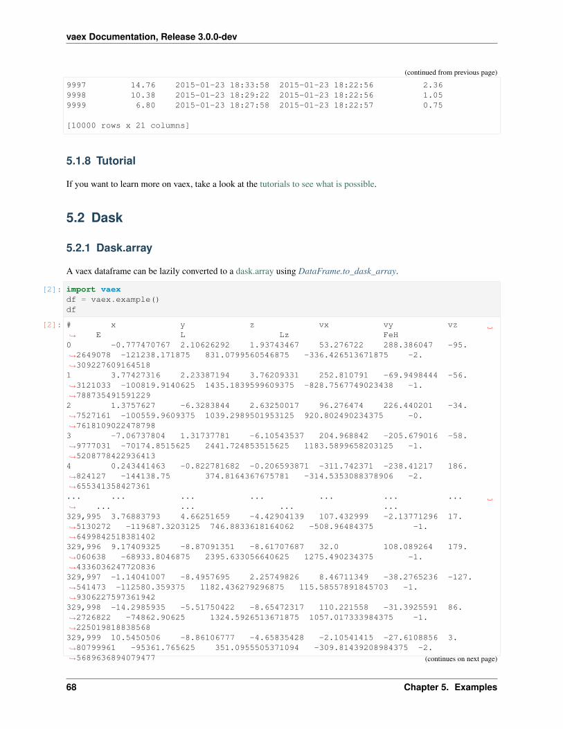
vaex Documentation, Release 3.0.0-dev
(continued from previous page)
9997 14.76 2015-01-23 18:33:58 2015-01-23 18:22:56 2.369998 10.38 2015-01-23 18:29:22 2015-01-23 18:22:56 1.059999 6.80 2015-01-23 18:27:58 2015-01-23 18:22:57 0.75
[10000 rows x 21 columns]
5.1.8 Tutorial
If you want to learn more on vaex, take a look at the tutorials to see what is possible.
5.2 Dask
5.2.1 Dask.array
A vaex dataframe can be lazily converted to a dask.array using DataFrame.to_dask_array.
[2]: import vaexdf = vaex.example()df
[2]: # x y z vx vy vz→˓ E L Lz FeH0 -0.777470767 2.10626292 1.93743467 53.276722 288.386047 -95.→˓2649078 -121238.171875 831.0799560546875 -336.426513671875 -2.→˓3092276091645181 3.77427316 2.23387194 3.76209331 252.810791 -69.9498444 -56.→˓3121033 -100819.9140625 1435.1839599609375 -828.7567749023438 -1.→˓7887354915912292 1.3757627 -6.3283844 2.63250017 96.276474 226.440201 -34.→˓7527161 -100559.9609375 1039.2989501953125 920.802490234375 -0.→˓76181090224787983 -7.06737804 1.31737781 -6.10543537 204.968842 -205.679016 -58.→˓9777031 -70174.8515625 2441.724853515625 1183.5899658203125 -1.→˓52087784229364134 0.243441463 -0.822781682 -0.206593871 -311.742371 -238.41217 186.→˓824127 -144138.75 374.8164367675781 -314.5353088378906 -2.→˓655341358427361... ... ... ... ... ... ...→˓ ... ... ... ...329,995 3.76883793 4.66251659 -4.42904139 107.432999 -2.13771296 17.→˓5130272 -119687.3203125 746.8833618164062 -508.96484375 -1.→˓6499842518381402329,996 9.17409325 -8.87091351 -8.61707687 32.0 108.089264 179.→˓060638 -68933.8046875 2395.633056640625 1275.490234375 -1.→˓4336036247720836329,997 -1.14041007 -8.4957695 2.25749826 8.46711349 -38.2765236 -127.→˓541473 -112580.359375 1182.436279296875 115.58557891845703 -1.→˓9306227597361942329,998 -14.2985935 -5.51750422 -8.65472317 110.221558 -31.3925591 86.→˓2726822 -74862.90625 1324.5926513671875 1057.017333984375 -1.→˓225019818838568329,999 10.5450506 -8.86106777 -4.65835428 -2.10541415 -27.6108856 3.→˓80799961 -95361.765625 351.0955505371094 -309.81439208984375 -2.→˓5689636894079477 (continues on next page)
68 Chapter 5. Examples

vaex Documentation, Release 3.0.0-dev
(continued from previous page)
[10]: # convert a set of columns in the dataframe to a 2d dask arrayA = df[['x', 'y', 'z']].to_dask_array()A
[10]: dask.array<vaex-df-d741baee-10eb-11ea-b19a, shape=(330000, 3), dtype=float64,→˓chunksize=(330000, 3), chunktype=numpy.ndarray>
[11]: import dask.array as da# lazily compute with daskr = da.sqrt(A[:,0]**2 + A[:,1]**2 + A[:,2]**2)r
[11]: dask.array<sqrt, shape=(330000,), dtype=float64, chunksize=(330000,), chunktype=numpy.→˓ndarray>
[12]: # materialize the datar_computed = r.compute()r_computed
[15]: # put it back in the dataframedf['r'] = r_computeddf
[15]: # x y z vx vy vz→˓ E L Lz FeH r0 -0.777470767 2.10626292 1.93743467 53.276722 288.386047 -95.→˓2649078 -121238.171875 831.0799560546875 -336.426513671875 -2.→˓309227609164518 2.96554503965535871 3.77427316 2.23387194 3.76209331 252.810791 -69.9498444 -56.→˓3121033 -100819.9140625 1435.1839599609375 -828.7567749023438 -1.→˓788735491591229 5.778292810490182 1.3757627 -6.3283844 2.63250017 96.276474 226.440201 -34.→˓7527161 -100559.9609375 1039.2989501953125 920.802490234375 -0.→˓7618109022478798 6.990796039502563 -7.06737804 1.31737781 -6.10543537 204.968842 -205.679016 -58.→˓9777031 -70174.8515625 2441.724853515625 1183.5899658203125 -1.→˓5208778422936413 9.4318427527075374 0.243441463 -0.822781682 -0.206593871 -311.742371 -238.41217 186.→˓824127 -144138.75 374.8164367675781 -314.5353088378906 -2.→˓655341358427361 0.8825613121347967... ... ... ... ... ... ...→˓ ... ... ... ...→˓...329,995 3.76883793 4.66251659 -4.42904139 107.432999 -2.13771296 17.→˓5130272 -119687.3203125 746.8833618164062 -508.96484375 -1.→˓6499842518381402 7.453831761514681329,996 9.17409325 -8.87091351 -8.61707687 32.0 108.089264 179.→˓060638 -68933.8046875 2395.633056640625 1275.490234375 -1.→˓4336036247720836 15.398412491068198329,997 -1.14041007 -8.4957695 2.25749826 8.46711349 -38.2765236 -127.→˓541473 -112580.359375 1182.436279296875 115.58557891845703 -1.→˓9306227597361942 8.864250273925633329,998 -14.2985935 -5.51750422 -8.65472317 110.221558 -31.3925591 86.→˓2726822 -74862.90625 1324.5926513671875 1057.017333984375 -1.→˓225019818838568 17.601047186042507
(continues on next page)
5.2. Dask 69
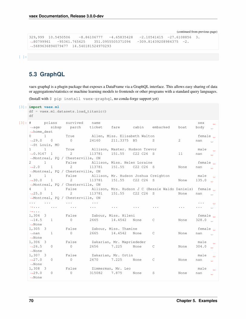
vaex Documentation, Release 3.0.0-dev
(continued from previous page)
329,999 10.5450506 -8.86106777 -4.65835428 -2.10541415 -27.6108856 3.→˓80799961 -95361.765625 351.0955505371094 -309.81439208984375 -2.→˓5689636894079477 14.540181524970293
[ ]:
5.3 GraphQL
vaex-graphql is a plugin package that exposes a DataFrame via a GraphQL interface. This allows easy sharing of dataor aggregations/statistics or machine learning models to frontends or other programs with a standard query languages.
(Install with $ pip install vaex-graphql, no conda-forge support yet)
[3]: import vaex.mldf = vaex.ml.datasets.load_titanic()df
[3]: # pclass survived name sex→˓age sibsp parch ticket fare cabin embarked boat body→˓home_dest0 1 True Allen, Miss. Elisabeth Walton female→˓29.0 0 0 24160 211.3375 B5 S 2 nan→˓St Louis, MO1 1 True Allison, Master. Hudson Trevor male→˓0.9167 1 2 113781 151.55 C22 C26 S 11 nan→˓Montreal, PQ / Chesterville, ON2 1 False Allison, Miss. Helen Loraine female→˓2.0 1 2 113781 151.55 C22 C26 S None nan→˓Montreal, PQ / Chesterville, ON3 1 False Allison, Mr. Hudson Joshua Creighton male→˓30.0 1 2 113781 151.55 C22 C26 S None 135.0→˓Montreal, PQ / Chesterville, ON4 1 False Allison, Mrs. Hudson J C (Bessie Waldo Daniels) female→˓25.0 1 2 113781 151.55 C22 C26 S None nan→˓Montreal, PQ / Chesterville, ON... ... ... ... ...→˓... ... ... ... ... ... ... ... ...→˓...1,304 3 False Zabour, Miss. Hileni female→˓14.5 1 0 2665 14.4542 None C None 328.0→˓None1,305 3 False Zabour, Miss. Thamine female→˓nan 1 0 2665 14.4542 None C None nan→˓None1,306 3 False Zakarian, Mr. Mapriededer male→˓26.5 0 0 2656 7.225 None C None 304.0→˓None1,307 3 False Zakarian, Mr. Ortin male→˓27.0 0 0 2670 7.225 None C None nan→˓None1,308 3 False Zimmerman, Mr. Leo male→˓29.0 0 0 315082 7.875 None S None nan→˓None
70 Chapter 5. Examples
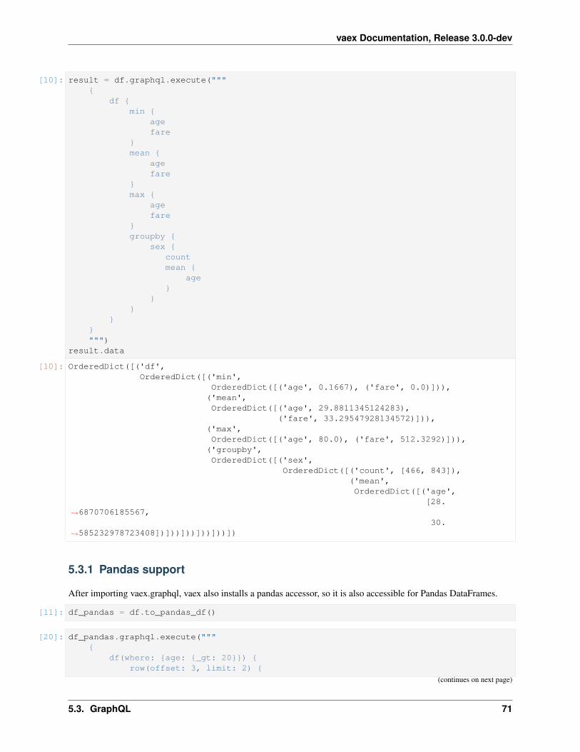
vaex Documentation, Release 3.0.0-dev
[10]: result = df.graphql.execute("""{
df {min {
agefare
}mean {
agefare
}max {
agefare
}groupby {
sex {countmean {
age}
}}
}}""")
result.data
[10]: OrderedDict([('df',OrderedDict([('min',
OrderedDict([('age', 0.1667), ('fare', 0.0)])),('mean',OrderedDict([('age', 29.8811345124283),
('fare', 33.29547928134572)])),('max',OrderedDict([('age', 80.0), ('fare', 512.3292)])),
('groupby',OrderedDict([('sex',
OrderedDict([('count', [466, 843]),('mean',OrderedDict([('age',
[28.→˓6870706185567,
30.→˓585232978723408])]))]))]))]))])
5.3.1 Pandas support
After importing vaex.graphql, vaex also installs a pandas accessor, so it is also accessible for Pandas DataFrames.
[11]: df_pandas = df.to_pandas_df()
[20]: df_pandas.graphql.execute("""{
df(where: {age: {_gt: 20}}) {row(offset: 3, limit: 2) {
(continues on next page)
5.3. GraphQL 71

vaex Documentation, Release 3.0.0-dev
(continued from previous page)
namesurvived
}}
}"""
).data
[20]: OrderedDict([('df',OrderedDict([('row',
[OrderedDict([('name', 'Anderson, Mr. Harry'),('survived', True)]),
OrderedDict([('name','Andrews, Miss. Kornelia Theodosia'),
('survived', True)])])]))])
5.3.2 Server
The easiest way to learn to use the GraphQL language/vaex interface is to launch a server, and play with the GraphiQLgraphical interface, its autocomplete, and the schema explorer.
We try to stay close to the Hasura API: https://docs.hasura.io/1.0/graphql/manual/api-reference/graphql-api/query.html
A server can be started from the command line:
$ python -m vaex.graphql myfile.hdf5
Or from within Python using df.graphql.serve
5.3.3 GraphiQL
See https://github.com/mariobuikhuizen/ipygraphql for a graphical widget, or a mybinder to try out a live example.
[ ]:
5.4 I/O Kung-Fu: get your data in and out of Vaex
5.4.1 Data input
Every project starts with reading in some data. Vaex supports several data sources:
• Binary file formats:
– HDF5
– Apache Arrow
– Apache Parquet
– FITS
• Text based file formats:
– CSV
72 Chapter 5. Examples

vaex Documentation, Release 3.0.0-dev
– ASCII
– JSON
• In-memory data representations:
– pandas DataFrames and everything that pandas can read
– Apache Arrow Tables
– numpy arrays
– Python dictionaries
– Single row DataFrames
The following examples show the best practices of getting your data in Vaex.
Binary file formats
If your data is already in one of the supported binary file formats (HDF5, Apache Arrow, Apache Parquet, FITS),opening it with Vaex rather simple:
[1]: import vaex
# Reading a HDF5 filedf_names = vaex.open('./data/io/sample_names_1.hdf5')df_names
[1]: # name age city0 John 17 Edinburgh1 Sally 33 Groningen
[2]: # Reading an arrow filedf_fruits = vaex.open('./data/io/sample_fruits.arrow')df_fruits
[2]: # fruit amount origin0 mango 5 Malaya1 banana 10 Ecuador2 orange 7 Spain
Opening such data is instantenous regardless of the file size on disk: Vaex will just memory-map the data instead ofreading it in memory. This is the optimal way of working with large datasets that are larger than available RAM.
If your data is contained within multiple files, one can open them all simultaneously like this:
[3]: df_names_all = vaex.open('./data/io/sample_names_*.hdf5')df_names_all
[3]: # name age city0 John 17 Edinburgh1 Sally 33 Groningen2 Maria 23 Caracas3 Monica 55 New York
Alternatively, one can use the open_many method to pass a list of files to open:
[4]: df_names_all = vaex.open_many(['./data/io/sample_names_1.hdf5','./data/io/sample_names_2.hdf5'])
df_names_all
5.4. I/O Kung-Fu: get your data in and out of Vaex 73

vaex Documentation, Release 3.0.0-dev
[4]: # name age city0 John 17 Edinburgh1 Sally 33 Groningen2 Maria 23 Caracas3 Monica 55 New York
The result will be a single DataFrame object containing all of the data coming from all files.
The data does not necessarily have to be local. With Vaex you can open a HDF5 file straight from Amazon’s S3:
[5]: df_from_s3 = vaex.open('s3://vaex/testing/xys.hdf5?anon=true')df_from_s3
[5]: # x y s0 1 3 51 2 4 6
In this case the data will be lazily downloaded and cached to the local machine. “Lazily downloaded” means that Vaexwill only download the portions of the data you really need. For example: imagine that we have a file hosted on S3 thathas 100 columns and 1 billion rows. Getting a preview of the DataFrame via print(df) for instance will downloadonly the first and last 5 rows. If we than proceed to make calculations or plots with only 5 columns, only the data fromthose columns will be downloaded and cached to the local machine.
By default, data that is streamed from S3 is cached at $HOME/.vaex/file-cache/s3, and thus successive accessis as fast as native disk access. One can also use the profile_name argument to use a specific S3 profile, whichwill than be passed to s3fs.core.S3FileSystem.
With Vaex one can also read-in parquet files:
[6]: # Reading a parquet filedf_cars = vaex.open('./data/io/sample_cars.parquet')df_cars
[6]: # car color year0 renault red 19961 audi black 20052 toyota blue 2000
Text based file formats
Datasets are still commonly stored in text-based file formats such as CSV. Since text-based file formats are notmemory-mappable, they have to be read in memory. If the contents of a CSV file fits into the available RAM, one cansimply do:
[7]: df_nba = vaex.from_csv('./data/io/sample_nba.csv', copy_index=False)df_nba
[7]: # city team player0 Indianopolis Pacers Reggie Miller1 Chicago Bulls Michael Jordan2 Boston Celtics Larry Bird
or alternatively:
[8]: df_nba = vaex.read_csv('./data/io/sample_nba_1.csv', copy_index=False)df_nba
74 Chapter 5. Examples

vaex Documentation, Release 3.0.0-dev
[8]: # city team player0 Indianopolis Pacers Reggie Miller1 Chicago Bulls Michael Jordan2 Boston Celtics Larry Bird
Vaex is using pandas for reading CSV files in the background, so one can pass any arguments to the vaex.from_csvor vaex.read_csv as one would pass to pandas.read_csv and specify for example separators, column namesand column types. The copy_index parameter specifies if the index column of the pandas DataFrame should beread as a regular column, or left out to save memory. In addition to this, if you specify the convert=True argument,the data will be automatically converted to an HDF5 file behind the scenes, thus freeing RAM and allowing you towork with your data in a memory-efficient, out-of-core manner.
If the CSV file is so large that it can not fit into RAM all at one time, one can convert the data to HDF5 simply by:
df = vaex.from_csv('./my_data/my_big_file.csv', convert=True, chunk_size=5_000_000)
When the above line is executed, Vaex will read the CSV in chunks, and convert each chunk to a temporary HDF5 fileon disk. All temporary files are then concatenated into a single HDF5 file, and the temporary files deleted. The size ofthe individual chunks to be read can be specified via the chunk_size argument. Note that this automatic conversionrequires free disk space of twice the final HDF5 file size.
It often happens that the data we need to analyse is spread over multiple CSV files. One can convert them to the HDF5file format like this:
[9]: list_of_files = ['./data/io/sample_nba_1.csv','./data/io/sample_nba_2.csv','./data/io/sample_nba_3.csv',]
# Convert each CSV file to HDF5for file in list_of_files:
df_tmp = vaex.from_csv(file, convert=True, copy_index=False)
The above code block converts in turn each CSV file to the HDF5 format. Note that the conversion will work regardlessof the file size of each individual CSV file, provided there is sufficient storage space.
Working with all of the data is now easy: just open all of the relevant HDF5 files as described above:
[10]: df = vaex.open('./data/io/sample_nba_*.csv.hdf5')df
[10]: # city team player0 Indianopolis Pacers Reggie Miller1 Chicago Bulls Michael Jordan2 Boston Celtics Larry Bird3 Los Angeles Lakers Kobe Bryant4 Toronto Raptors Vince Carter5 Philadelphia 76ers Allen Iverson6 San Antonio Spurs Tim Duncan
One can than additionally export this combined DataFrame to a single HDF5 file. This should lead to minor perfor-mance improvements.
[11]: df.export('./data/io/sample_nba_combined.hdf5')
It is also common the data to be stored in JSON files. To read such data in Vaex one can do:
5.4. I/O Kung-Fu: get your data in and out of Vaex 75

vaex Documentation, Release 3.0.0-dev
[12]: df_isles = vaex.from_json('./data/io/sample_isles.json', orient='table', copy_→˓index=False)df_isles
[12]: # isle size_sqkm0 Easter Island 163.61 Fiji 18.3332 Tortuga 178.7
This is a convenience method which simply wraps pandas.read_json, so the same arguments and file readingstrategy applies. If the data is distributed amongs multiple JSON files, one can apply a similar strategy as in the caseof multiple CSV files: read each JSON file with the vaex.from_json method, convert it to a HDF5 or Arrow fileformat. Than use vaex.open or vaex.open_many methods to open all the converted files as a single DataFrame.
To learn more about different options of exporting data with Vaex, please read the next section below.
In-memory data representations
One can construct a Vaex DataFrame from a variety of in-memory data representations. Such a common operationis converting a pandas into a Vaex DataFrame. Let us read in a CSV file with pandas and than convert it to a VaexDataFrame:
[13]: import pandas as pd
pandas_df = pd.read_csv('./data/io/sample_nba.csv')pandas_df
[13]: city team player0 Indianopolis Pacers Reggie Miller1 Chicago Bulls Michael Jordan2 Boston Celtics Larry Bird
[14]: df = vaex.from_pandas(df=pandas_df, copy_index=True)df
[14]: # city team player index0 Indianopolis Pacers Reggie Miller 01 Chicago Bulls Michael Jordan 12 Boston Celtics Larry Bird 2
The copy_index argument specifies whether the index column of a pandas DataFrame should be imported into theVaex DataFrame. Converting a pandas into a Vaex DataFrame is particularly useful since pandas can read data froma large variety of file formats. For instance, we can use pandas to read data from a database, and then pass it to Vaexlike so:
import vaeximport pandas as pdimport sqlalchemy
connection_string = 'postgresql://readonly:' + 'my_password' + '@server.company.com:→˓1234/database_name'engine = sqlalchemy.create_engine(connection_string)
pandas_df = pd.read_sql_query('SELECT * FROM MYTABLE', con=engine)df = vaex.from_pandas(pandas_df, copy_index=False)
Another example is using pandas to read in SAS files:
76 Chapter 5. Examples

vaex Documentation, Release 3.0.0-dev
[15]: pandas_df = pd.read_sas('./data/io/sample_airline.sas7bdat')df = vaex.from_pandas(pandas_df, copy_index=False)df
[15]: # YEAR Y W R L→˓ K0 1948.0 1.2139999866485596 0.24300000071525574 0.1454000025987625 1.→˓4149999618530273 0.61199998855590821 1949.0 1.3539999723434448 0.25999999046325684 0.21809999644756317 1.→˓3839999437332153 0.55900001525878912 1950.0 1.569000005722046 0.27799999713897705 0.3156999945640564 1.→˓3880000114440918 0.57300001382827763 1951.0 1.9479999542236328 0.296999990940094 0.39399999380111694 1.→˓5499999523162842 0.56400001049041754 1952.0 2.265000104904175 0.3100000023841858 0.35589998960494995 1.→˓8020000457763672 0.5740000009536743... ... ... ... ... ...→˓ ...27 1975.0 18.72100067138672 1.246999979019165 0.23010000586509705 5.→˓7220001220703125 9.06200027465820328 1976.0 19.25 1.375 0.3452000021934509 5.→˓76200008392334 8.2620000839233429 1977.0 20.64699935913086 1.5440000295639038 0.45080000162124634 5.→˓876999855041504 7.47399997711181630 1978.0 22.72599983215332 1.7029999494552612 0.5877000093460083 6.→˓107999801635742 7.10400009155273431 1979.0 23.618999481201172 1.7790000438690186 0.534600019454956 6.→˓8520002365112305 6.874000072479248
One can read in an arrow table as a Vaex DataFrame in a similar manner. Let us first use pyarrow to read in a CSV fileas an arrow table.
[16]: import pyarrow.csv
arrow_table = pyarrow.csv.read_csv('./data/io/sample_nba.csv')arrow_table
[16]: pyarrow.Tablecity: stringteam: stringplayer: string
Once we have the arrow table, converting it to a DataFrame is simple:
[17]: df = vaex.from_arrow_table(arrow_table)df
[17]: # city team player0 Indianopolis Pacers Reggie Miller1 Chicago Bulls Michael Jordan2 Boston Celtics Larry Bird
It also common to construct a Vaex DataFrame from numpy arrays. That can be done like this:
[18]: import numpy as np
x = np.arange(2)y = np.array([10, 20])z = np.array(['dog', 'cat'])
(continues on next page)
5.4. I/O Kung-Fu: get your data in and out of Vaex 77

vaex Documentation, Release 3.0.0-dev
(continued from previous page)
df_numpy = vaex.from_arrays(x=x, y=y, z=z)df_numpy
[18]: # x y z0 0 10 dog1 1 20 cat
Constructing a DataFrame from a Python dict is also straight-forward:
[19]: # Construct a DataFrame from Python dictionarydata_dict = dict(x=[2, 3], y=[30, 40], z=['cow', 'horse'])
df_dict = vaex.from_dict(data_dict)df_dict
[19]: # x y z0 2 30 cow1 3 40 horse
At times, one may need to create a single row DataFrame. Vaex has a convenience method which takes individualelements (scalars) and creates the DataFrame:
[20]: df_single_row = vaex.from_scalars(x=4, y=50, z='mouse')df_single_row
[20]: # x y z0 4 50 mouse
Finally, we can choose to concatenate different DataFrames, without any memory penalties like so:
[21]: df = vaex.concat([df_numpy, df_dict, df_single_row])df
[21]: # x y z0 0 10 dog1 1 20 cat2 2 30 cow3 3 40 horse4 4 50 mouse
5.4.2 Data export
One can export Vaex DataFrames to multiple file or in-memory data representations:
• Binary file formats:
– HDF5
– Apache Arrow
– Apache Parquet
– FITS
• Text based file formats:
– CSV
78 Chapter 5. Examples

vaex Documentation, Release 3.0.0-dev
– ASCII
• In-memory data representations:
– DataFrames:
* panads DataFrame
* Apache Arrow Table
* numpy arrays
* Dask arrays
* Python dictionaries
* Python items list ( a list of (‘column_name’, data) tuples)
– Expressions:
* panads Series
* numpy array
* Dask array
* Python list
Binary file formats
The most efficient way to store data on disk when you work with Vaex is to use binary file formats. Vaex can export aDataFrame to HDF5, Apache Arrow, Apache Parquet and FITS:
[22]: df.export_hdf5('./data/io/output_data.hdf5')df.export_arrow('./data/io/output_data.arrow')df.export_parquet('./data/io/output_data.parquet')
Alternatively, one can simply use:
[23]: df.export('./data/io/output_data.hdf5')df.export('./data/io/output_data.arrow')df.export('./data/io/output_data.parquet')
where Vaex will determine the file format of the based on the specified extension of the file name. If the extension isnot recognized, an exception will be raised.
If your data is large, i.e. larger than the available RAM, we recomment exporting to HDF5.
Text based file format
At times, it may be useful to export the data to disk in a text based file format such as CSV. In that case one can simplydo:
[24]: df.export_csv('./data/io/output_data.csv') # `chunk_size` has a default value of 1_→˓000_000
The df.export_csv method is using pandas_df.to_csv behind the scenes, and thus one can pass any argu-ment to df.export_csv as would to pandas_df.to_csv. The data is exported in chunks and the size of thosechunks can be specified by the chunk_size argument in df.export_csv. In this way, data that is too large to fitin RAM can be saved to disk.
5.4. I/O Kung-Fu: get your data in and out of Vaex 79
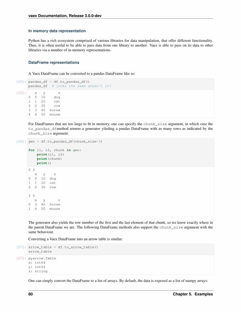
vaex Documentation, Release 3.0.0-dev
In memory data representation
Python has a rich ecosystem comprised of various libraries for data manipulation, that offer different functionality.Thus, it is often useful to be able to pass data from one library to another. Vaex is able to pass on its data to otherlibraries via a number of in-memory representations.
DataFrame representations
A Vaex DataFrame can be converted to a pandas DataFrame like so:
[25]: pandas_df = df.to_pandas_df()pandas_df # looks the same doesn't it?
[25]: x y z0 0 10 dog1 1 20 cat2 2 30 cow3 3 40 horse4 4 50 mouse
For DataFrames that are too large to fit in memory, one can specify the chunk_size argument, in which case theto_pandas_dfmethod returns a generator yileding a pandas DataFrame with as many rows as indicated by thechunk_size argument:
[26]: gen = df.to_pandas_df(chunk_size=3)
for i1, i2, chunk in gen:print(i1, i2)print(chunk)print()
0 3x y z
0 0 10 dog1 1 20 cat2 2 30 cow
3 5x y z
0 3 40 horse1 4 50 mouse
The generator also yields the row number of the first and the last element of that chunk, so we know exactly where inthe parent DataFrame we are. The following DataFrame methods also support the chunk_size argument with thesame behaviour.
Converting a Vaex DataFrame into an arrow table is similar:
[27]: arrow_table = df.to_arrow_table()arrow_table
[27]: pyarrow.Tablex: int64y: int64z: string
One can simply convert the DataFrame to a list of arrays. By default, the data is exposed as a list of numpy arrays:
80 Chapter 5. Examples

vaex Documentation, Release 3.0.0-dev
[28]: arrays = df.to_arrays()arrays
[28]: [array([0, 1, 2, 3, 4]),array([10, 20, 30, 40, 50]),array(['dog', 'cat', 'cow', 'horse', 'mouse'], dtype=object)]
By specifying the array_type argument, one can choose whether the data will be represented by numpy arrays,xarrays, or Python lists.
[29]: arrays = df.to_arrays(array_type='xarray')arrays # list of xarrays
[29]: [<xarray.DataArray (dim_0: 5)>array([0, 1, 2, 3, 4])Dimensions without coordinates: dim_0, <xarray.DataArray (dim_0: 5)>array([10, 20, 30, 40, 50])Dimensions without coordinates: dim_0, <xarray.DataArray (dim_0: 5)>array(['dog', 'cat', 'cow', 'horse', 'mouse'], dtype=object)Dimensions without coordinates: dim_0]
[30]: arrays = df.to_arrays(array_type='list')arrays # list of lists
[30]: [[0, 1, 2, 3, 4],[10, 20, 30, 40, 50],['dog', 'cat', 'cow', 'horse', 'mouse']]
Keeping it close to pure Python, one can export a Vaex DataFrame as a dictionary. The same array_type keywordargument applies here as well:
[31]: d_dict = df.to_dict(array_type='numpy')d_dict
[31]: {'x': array([0, 1, 2, 3, 4]),'y': array([10, 20, 30, 40, 50]),'z': array(['dog', 'cat', 'cow', 'horse', 'mouse'], dtype=object)}
Alternatively, one can also convert a DataFrame to a list of tuples, were the first element of the tuple is the columnname, while the second element is the array representation of the data.
[32]: # Get a single item listitems = df.to_items(array_type='list')items
[32]: [('x', [0, 1, 2, 3, 4]),('y', [10, 20, 30, 40, 50]),('z', ['dog', 'cat', 'cow', 'horse', 'mouse'])]
As mentioned earlier, with all of the above example, one can use the chunk_size argument which creates a gener-ator, yielding a portion of the DataFrame in the specified format. In the case of .to_dict method:
[33]: gen = df.to_dict(array_type='list', chunk_size=2)
for i1, i2, chunk in gen:print(i1, i2, chunk)
0 2 {'x': [0, 1], 'y': [10, 20], 'z': ['dog', 'cat']}2 4 {'x': [2, 3], 'y': [30, 40], 'z': ['cow', 'horse']}4 5 {'x': [4], 'y': [50], 'z': ['mouse']}
5.4. I/O Kung-Fu: get your data in and out of Vaex 81

vaex Documentation, Release 3.0.0-dev
Last but not least, a Vaex DataFrame can be lazily exposed as a Dask array:
[34]: dask_arrays = df[['x', 'y']].to_dask_array() # String support coming soondask_arrays
[34]: dask.array<vaex-df-899d5254-8abb-11ea-afee, shape=(5, 2), dtype=int64, chunksize=(5,→˓2), chunktype=numpy.ndarray>
Expression representations
A single Vaex Expression can be also converted to a variety of in-memory representations:
[35]: # pandas Seriesx_series = df.x.to_pandas_series()x_series
[35]: 0 01 12 23 34 4dtype: int64
[36]: # numpy arrayx_numpy = df.x.to_numpy()x_numpy
[36]: array([0, 1, 2, 3, 4])
[37]: # Python listx_list = df.x.tolist()x_list
[37]: [0, 1, 2, 3, 4]
[38]: # Dask arrayx_dask_array = df.x.to_dask_array()x_dask_array
[38]: dask.array<vaex-expression-89a70920-8abb-11ea-afee, shape=(5,), dtype=int64,→˓chunksize=(5,), chunktype=numpy.ndarray>
5.5 Machine Learning (basic): the Iris dataset
While vaex.ml does not yet implement predictive models, we provide wrappers to powerful libraries (e.g. Scikit-learn, xgboost) and make them work efficiently with vaex. vaex.ml does implement a variety of standard datatransformers (e.g. PCA, numerical scalers, categorical encoders) and a very efficient KMeans algorithm that take fulladvantage of vaex.
The following is a simple example on use of vaex.ml. We will be using the well known Iris dataset, and we will useit to build a model which distinguishes between the three Irish species (Iris setosa, Iris virginica and Iris versicolor).
Lets start by importing the common libraries, load and inspect the data.
82 Chapter 5. Examples

vaex Documentation, Release 3.0.0-dev
[1]: import vaeximport vaex.ml
import pylab as plt
df = vaex.ml.datasets.load_iris()df
[1]: # sepal_length sepal_width petal_length petal_width class_0 5.9 3.0 4.2 1.5 11 6.1 3.0 4.6 1.4 12 6.6 2.9 4.6 1.3 13 6.7 3.3 5.7 2.1 24 5.5 4.2 1.4 0.2 0... ... ... ... ... ...145 5.2 3.4 1.4 0.2 0146 5.1 3.8 1.6 0.2 0147 5.8 2.6 4.0 1.2 1148 5.7 3.8 1.7 0.3 0149 6.2 2.9 4.3 1.3 1
Splitting the data into train and test steps should be done immediately, before any manipulation is done on the data.vaex.ml contains a train_test_split method which creates shallow copies of the main DataFrame, meaningthat no extra memory is used when defining train and test sets. Note that the train_test_split method does anordered split of the main DataFrame to create the two sets. In some cases, one may need to shuffle the data.
If shuffling is required, we recommend the following:
df.export("shuffled", shuffle=True)df = vaex.open("shuffled.hdf5)df_train, df_test = df.ml.train_test_split(test_size=0.2)
In the present scenario, the dataset is already shuffled, so we can simply do the split right away.
[2]: # Orderd split in train and testdf_train, df_test = df.ml.train_test_split(test_size=0.2)
/Users/jovan/PyLibrary/vaex/packages/vaex-core/vaex/ml/__init__.py:209: UserWarning:→˓Make sure the DataFrame is shuffledwarnings.warn('Make sure the DataFrame is shuffled')
As this is a very simple tutorial, we will just use the columns already provided as features for training the model.
[3]: features = df_train.column_names[:4]features
[3]: ['sepal_length', 'sepal_width', 'petal_length', 'petal_width']
5.5.1 PCA
The vaex.ml module contains several classes for dataset transformations that are commonly used to pre-process dataprior to building a model. These include numerical feature scalers, category encoders, and PCA transformations. Wehave adopted the scikit-learn API, meaning that all transformers have the .fit and .transform methods.
Let’s use apply a PCA transformation on the training set. There is no need to scale the data beforehand, since the PCAalso normalizes the data.
5.5. Machine Learning (basic): the Iris dataset 83

vaex Documentation, Release 3.0.0-dev
[4]: pca = vaex.ml.PCA(features=features, n_components=4)df_train = pca.fit_transform(df_train)df_train
[4]: # sepal_length sepal_width petal_length petal_width class_ PCA_0→˓ PCA_1 PCA_2 PCA_30 5.4 3.0 4.5 1.5 1 -0.→˓5819340944906611 -0.5192084328455534 -0.4079706950207428 -0.228433256583780221 4.8 3.4 1.6 0.2 0 2.→˓628040487885542 -0.05578001049524599 -0.09961452867004605 -0.149605897563429352 6.9 3.1 4.9 1.5 1 -1.→˓438496521671396 0.5307778852279289 0.32322065776316616 -0.→˓00664789679919497443 4.4 3.2 1.3 0.2 0 3.→˓00633586736142 -0.41909744036887703 -0.17571839830952185 -0.054205415158371074 5.6 2.8 4.9 2.0 2 -1.→˓1948465297428466 -0.6200295372229213 -0.4751905348367903 0.08724845774327505... ... ... ... ... ... ...→˓ ... ... ...115 5.2 3.4 1.4 0.2 0 2.→˓6608856211270933 0.2619681501203415 0.12886483875694454 0.06429707648769989116 5.1 3.8 1.6 0.2 0 2.→˓561545765055359 0.4288927940763031 -0.18633294617759266 -0.20573646329612738117 5.8 2.6 4.0 1.2 1 -0.→˓22075578997244774 -0.40152336651555137 0.25417836518749715 0.04952191889168374118 5.7 3.8 1.7 0.3 0 2.→˓23068249078231 0.826166758833374 0.07863720599424912 0.→˓0004035597987264161119 6.2 2.9 4.3 1.3 1 -0.→˓6256358184862005 0.023930474333675168 0.21203674475657858 -0.→˓0077954052328795265
The result of pca .fit_transform method is a shallow copy of the DataFrame which contains the resultingcolumns of the transformation, in this case the PCA components, as virtual columns. This means that the trans-formed DataFrame takes no memory at all! So while this example is made with only 120 sample, this would work inthe same way even for millions or billions of samples.
5.5.2 Gradient boosting trees
Now let’s train a gradient boosting model. While vaex.ml does not currently include this type of models, wesupport the popular boosted trees libraries xgboost, lightgbm, and catboost. In this tutorial we will use the lightgbmclassifier.
[9]: import lightgbmimport vaex.ml.sklearn
# Features on which to train the modeltrain_features = df_train.get_column_names(regex='PCA_.*')# The target columntarget = 'class_'
# Instantiate the LightGBM Classifierbooster = lightgbm.sklearn.LGBMClassifier(num_leaves=5,
max_depth=5,n_estimators=100,random_state=42)
(continues on next page)
84 Chapter 5. Examples

vaex Documentation, Release 3.0.0-dev
(continued from previous page)
# Make it a vaex transformer (for the automagic pipeline and lazy predictions)model = vaex.ml.sklearn.SKLearnPredictor(features=train_features,
target=target,model=booster,prediction_name='prediction')
# Train and predictmodel.fit(df=df_train)df_train = model.transform(df=df_train)
df_train
[9]: # sepal_length sepal_width petal_length petal_width class_ PCA_0→˓ PCA_1 PCA_2 PCA_3→˓prediction0 5.4 3.0 4.5 1.5 1 -0.→˓5819340944906611 -0.5192084328455534 -0.4079706950207428 -0.22843325658378022→˓ 11 4.8 3.4 1.6 0.2 0 2.→˓628040487885542 -0.05578001049524599 -0.09961452867004605 -0.→˓14960589756342935 02 6.9 3.1 4.9 1.5 1 -1.→˓438496521671396 0.5307778852279289 0.32322065776316616 -0.→˓0066478967991949744 13 4.4 3.2 1.3 0.2 0 3.→˓00633586736142 -0.41909744036887703 -0.17571839830952185 -0.→˓05420541515837107 04 5.6 2.8 4.9 2.0 2 -1.→˓1948465297428466 -0.6200295372229213 -0.4751905348367903 0.08724845774327505→˓ 2... ... ... ... ... ... ...→˓ ... ... ... ...115 5.2 3.4 1.4 0.2 0 2.→˓6608856211270933 0.2619681501203415 0.12886483875694454 0.06429707648769989→˓ 0116 5.1 3.8 1.6 0.2 0 2.→˓561545765055359 0.4288927940763031 -0.18633294617759266 -0.→˓20573646329612738 0117 5.8 2.6 4.0 1.2 1 -0.→˓22075578997244774 -0.40152336651555137 0.25417836518749715 0.04952191889168374→˓ 1118 5.7 3.8 1.7 0.3 0 2.→˓23068249078231 0.826166758833374 0.07863720599424912 0.→˓0004035597987264161 0119 6.2 2.9 4.3 1.3 1 -0.→˓6256358184862005 0.023930474333675168 0.21203674475657858 -0.→˓0077954052328795265 1
Notice that after training the model, we use the .transform method to obtain a shallow copy of the DataFramewhich contains the prediction of the model, in a form of a virtual column. This makes it easy to evaluate the model,and easily create various diagnostic plots. If required, one can call the .predict method, which will result in anin-memory numpy.array housing the predictions.
5.5. Machine Learning (basic): the Iris dataset 85

vaex Documentation, Release 3.0.0-dev
5.5.3 Automatic pipelines
Assuming we are happy with the performance of the model, we can continue and apply our transformations andmodel to the test set. Unlike other libraries, we do not need to explicitly create a pipeline here in order to propagatethe transformations. In fact, with vaex and vaex.ml, a pipeline is automatically being created as one is doing theexploration of the data. Each vaex DataFrame contains a state, which is a (serializable) object containing informationof all transformations applied to the DataFrame (filtering, creation of new virtual columns, transformations).
Recall that the outputs of both the PCA transformation and the boosted model were in fact virtual columns, and thusare stored in the state of df_train. All we need to do, is to apply this state to another similar DataFrame (e.g. thetest set), and all the changes will be propagated.
[6]: state = df_train.state_get()df_test.state_set(state)
df_test
[6]: # sepal_length sepal_width petal_length petal_width class_ PCA_0→˓ PCA_1 PCA_2 PCA_3→˓prediction0 5.9 3.0 4.2 1.5 1 -0.→˓4978687101343986 -0.11289245880584761 -0.11962601206069637 0.0625954090178564→˓ 11 6.1 3.0 4.6 1.4 1 -0.→˓8754765898560835 -0.03902402119573594 0.022944044447894815 -0.14143773065379384→˓ 12 6.6 2.9 4.6 1.3 1 -1.→˓0228803632878913 0.2503709022470443 0.4130613754204865 -0.→˓030391911559003282 13 6.7 3.3 5.7 2.1 2 -2.→˓2544508624315838 0.3431374410700749 -0.28908707579214765 -0.07059175451207655→˓ 24 5.5 4.2 1.4 0.2 0 2.→˓632289228948536 1.020394958612415 -0.20769510079946696 -0.→˓13744144140286718 0... ... ... ... ... ... ...→˓ ... ... ... ...25 5.5 2.5 4.0 1.3 1 -0.→˓16189655085432594 -0.6871827581512436 0.09773053160021669 0.07093166682594204→˓ 126 5.8 2.7 3.9 1.2 1 -0.→˓12526327170089271 -0.3148233189949767 0.19720893202789733 0.060419826927667064→˓ 127 4.4 2.9 1.4 0.2 0 2.→˓8918941837640526 -0.6426744898497139 0.006171795874510444 0.→˓007700652884580328 028 4.5 2.3 1.3 0.3 0 2.→˓850207707200544 -0.9710397723109179 0.38501428492268475 0.377723418991853→˓ 029 6.9 3.2 5.7 2.3 2 -2.→˓405639277483925 0.4027072938482219 -0.22944817803540973 0.17443211711742812→˓ 2
5.5.4 Production
Now df_test contains all the transformations we applied on the training set (df_train), including the modelprediction. The transfer of state from one DataFrame to another can be extremely valuable for putting models in
86 Chapter 5. Examples

vaex Documentation, Release 3.0.0-dev
production.
5.5.5 Performance
Finally, let’s check the model performance.
[7]: from sklearn.metrics import accuracy_score
acc = accuracy_score(y_true=df_test.class_.values, y_pred=df_test.prediction.values)acc *= 100.print(f'Test set accuracy: {acc}%')
Test set accuracy: 100.0%
The model get perfect accuracy of 100%. This is not surprising as this problem is rather easy: doing a PCA transfor-mation on the features nicely separates the 3 flower species. Plotting the first two PCA axes, and colouring the samplesaccording to their class already shows an almost perfect separation.
[8]: plt.figure(figsize=(8, 4))df_test.scatter(df_test.PCA_0, df_test.PCA_1, c_expr=df_test.class_, s=50)plt.show()
5.6 Machine Learning (advanced): the Titanic dataset
In the following is a more involved machine learning example, in which we will use a larger variety of method inveax to do data cleaning, feature engineering, pre-processing and finally to train a couple of models. To do this, wewill use the well known Titanic dataset. Our task is to predict which passengers are more likely to have survived thedisaster.
Before we begin, thare there are two important notes to consider: - The following example is not to provide a compet-itive score for any competitions that might use the Titanic dataset. It’s primary goal is to show how various methodsprovided by vaex and vaex.ml can be used to clean data, create new features, and do general data manipulations ina machine learning context. - While the Titanic dataset is rather small in side, all the methods and operations presentedin the solution below will work on a dataset of arbitrary size, as long as it fits on the hard-drive of your machine.
Now, with that out of the way, let’s get started!
5.6. Machine Learning (advanced): the Titanic dataset 87

vaex Documentation, Release 3.0.0-dev
[1]: import vaeximport vaex.ml
import numpy as npimport pylab as plt
5.6.1 Adjusting matplotlib parmeters
Intermezzo: we modify some of the matplotlib default settings, just to make the plots a bit more legible.
[2]: SMALL_SIZE = 12MEDIUM_SIZE = 14BIGGER_SIZE = 16
plt.rc('font', size=SMALL_SIZE) # controls default text sizesplt.rc('axes', titlesize=SMALL_SIZE) # fontsize of the axes titleplt.rc('axes', labelsize=MEDIUM_SIZE) # fontsize of the x and y labelsplt.rc('xtick', labelsize=SMALL_SIZE) # fontsize of the tick labelsplt.rc('ytick', labelsize=SMALL_SIZE) # fontsize of the tick labelsplt.rc('legend', fontsize=SMALL_SIZE) # legend fontsizeplt.rc('figure', titlesize=BIGGER_SIZE) # fontsize of the figure title
5.6.2 Get the data
First of all we need to read in the data. Since the Titanic dataset is quite well known for trying out different classifi-cation algorithms, as well as commonly used as a teaching tool for aspiring data scientists, it ships (no pun intended)together with vaex.ml. So let’s read it in, see the description of its contents, and get a preview of the data.
[3]: # Load the titanic datasetdf = vaex.ml.datasets.load_titanic()
# See the descriptiondf.info()
<IPython.core.display.HTML object>
<IPython.core.display.HTML object>
Shuffling
From the preview of the DataFrame we notice that the data is sorted alphabetically by name and by passenger class.Thus we need to shuffle it before we split it into train and test sets.
[4]: # The dataset is ordered, so let's shuffle itdf = df.sample(frac=1, random_state=31)
Shuffling for large datasets
As mentioned in The ML introduction tutorial, shuffling large datasets in-memory is not a good idea. In case you workwith a large dataset, consider shuffling while exporting:
88 Chapter 5. Examples

vaex Documentation, Release 3.0.0-dev
df.export("shuffled", shuffle=True)df = vaex.open("shuffled.hdf5)df_train, df_test = df.ml.train_test_split(test_size=0.2)
Split into train and test
Once the data is shuffled, let’s split it into train and test sets. The test set will comprise 20% of the data. Note that wedo not shuffle the data for you, since vaex cannot assume your data fits into memory, you are responsible for eitherwriting it in shuffled order on disk, or shuffle it in memory (the previous step).
[5]: # Train and test split, no shuffling occursdf_train, df_test = df.ml.train_test_split(test_size=0.2, verbose=False)
Sanity checks
Before we move on to process the data, let’s verify that our train and test sets are “similar” enough. We will not bevery rigorous here, but just look at basic statistics of some of the key features.
For starters, let’s check that the fraction of survivals is similar between the train and test sets.
[6]: # Inspect the target variabletrain_survived_value_counts = df_train.survived.value_counts()test_survived_value_counts = df_test.survived.value_counts()
plt.figure(figsize=(12, 4))
plt.subplot(121)train_survived_value_counts.plot.bar()train_sex_ratio = train_survived_value_counts[True]/train_survived_value_counts[False]plt.title(f'Train set: survivied ratio: {train_sex_ratio:.2f}')plt.ylabel('Number of passengers')
plt.subplot(122)test_survived_value_counts.plot.bar()test_sex_ratio = test_survived_value_counts[True]/test_survived_value_counts[False]plt.title(f'Test set: surived ratio: {test_sex_ratio:.2f}')
plt.tight_layout()plt.show()
5.6. Machine Learning (advanced): the Titanic dataset 89

vaex Documentation, Release 3.0.0-dev
Next up, let’s check whether the ratio of male to female passengers is not too dissimilar between the two sets.
[7]: # Check the sex balancetrain_sex_value_counts = df_train.sex.value_counts()test_sex_value_counts = df_test.sex.value_counts()
plt.figure(figsize=(12, 4))
plt.subplot(121)train_sex_value_counts.plot.bar()train_sex_ratio = train_sex_value_counts['male']/train_sex_value_counts['female']plt.title(f'Train set: male vs female ratio: {train_sex_ratio:.2f}')plt.ylabel('Number of passengers')
plt.subplot(122)test_sex_value_counts.plot.bar()test_sex_ratio = test_sex_value_counts['male']/test_sex_value_counts['female']plt.title(f'Test set: male vs female ratio: {test_sex_ratio:.2f}')
plt.tight_layout()plt.show()
Finally, lets check that the relative number of passenger per class is similar between the train and test sets.
[8]: # Check the class balancetrain_pclass_value_counts = df_train.pclass.value_counts()test_pclass_value_counts = df_test.pclass.value_counts()
(continues on next page)
90 Chapter 5. Examples

vaex Documentation, Release 3.0.0-dev
(continued from previous page)
plt.figure(figsize=(12, 4))
plt.subplot(121)plt.title('Train set: passenger class')train_pclass_value_counts.plot.bar()
plt.subplot(122)plt.title('Test set: passenger class')test_pclass_value_counts.plot.bar()
plt.tight_layout()plt.show()
From the above diagnostics, we are satisfied that, at least in these few categories, the train and test are similar enough,and we can move forward.
5.6.3 Feature engineering
In this section we will use vaex to create meaningful features that will be used to train a classification model. To startwith, let’s get a high level overview of the training data.
[9]: df_train.describe()
[9]: pclass survived name sex age \dtype int64 bool str str float64count 1047 1047 1047 1047 841NA 0 0 0 0 206mean 2.3075453677172875 0.3744030563514804 -- -- 29.565299286563608std 0.833269 0.483968 -- -- 14.162min 1 False -- -- 0.1667max 3 True -- -- 80
sibsp parch ticket fare \dtype int64 int64 str float64count 1047 1047 1047 1046NA 0 0 0 1mean 0.5100286532951289 0.3982808022922636 -- 32.926091013384294std 1.07131 0.890852 -- 50.6783min 0 0 -- 0max 8 9 -- 512.329
(continues on next page)
5.6. Machine Learning (advanced): the Titanic dataset 91

vaex Documentation, Release 3.0.0-dev
(continued from previous page)
cabin embarked boat body home_destdtype str str str float64 strcount 233 1046 380 102 592NA 814 1 667 945 455mean -- -- -- 159.6764705882353 --std -- -- -- 96.2208 --min -- -- -- 1 --max -- -- -- 327 --
Imputing
We notice that there are 3 columns that have missing data, so our first task will be to impute the missing values withsuitable substitutes. This is our strategy:
• age: impute with the median age value
• fare: impute with the mean fare of the 5 most common values.
• cabin: impute with “M” for “Missing”
• Embarked: Impute with with the most common value.
[10]: # Handle missing values
# Age - just do the mean of the training set for nowmedian_age = df_train.percentile_approx(expression='age', percentage=50.0)df_train['age'] = df_train.age.fillna(value=median_age)
# Fare: the mean of the 5 most common ticket prices.fill_fares = df_train.fare.value_counts(dropna=True)fill_fare = fill_fares.iloc[:5].index.values.mean()df_train['fare'] = df_train.fare.fillna(value=fill_fare)
# Cabing: this is a string column so let's mark it as "M" for "Missing"df_train['cabin'] = df_train.cabin.fillna(value='M')
# Embarked: Similar as for Cabin, let's mark the missing values with "U" for unknownfill_embarked = df_train.embarked.value_counts(dropna=True).index[0]df_train['embarked'] = df_train.embarked.fillna(value=fill_embarked)
String processing
Next up, let’s engineer some new, more meaningful features out of the “raw” data that is present in the dataset. Startingwith the name of the passengers, we are going to extract the titles, as well as we are going to count the number ofwords a name contains. These features can be a loose proxy to the age and status of the passengers.
[11]: # Engineer features from the names
# Titlesdf_train['name_title'] = df_train['name'].str.replace('.* ([A-Z][a-z]+)\..*', "\\1",→˓regex=True)display(df_train['name_title'])
# Number of words in the name
(continues on next page)
92 Chapter 5. Examples

vaex Documentation, Release 3.0.0-dev
(continued from previous page)
df_train['name_num_words'] = df_train['name'].str.count("[ ]+", regex=True) + 1display(df_train['name_num_words'])
Expression = name_titleLength: 1,047 dtype: str (column)---------------------------------
0 Mr1 Mr2 Mrs3 Miss4 Mr...
1042 Master1043 Mrs1044 Master1045 Mr1046 Mr
Expression = name_num_wordsLength: 1,047 dtype: int64 (column)-----------------------------------
0 31 42 53 44 4...
1042 41043 61044 41045 41046 3
From the cabin colum, we will engineer 3 features: - “deck”: extacting the deck on which the cabin is located, whichis encoded in each cabin value; - “multi_cabin: a boolean feature indicating whether a passenger is allocated morethan one cabin - “has_cabin”: since there were plenty of values in the original cabin column that had missing values,we are just going to build a feature which tells us whether a passenger had an assigned cabin or not.
[12]: # Extract the deckdf_train['deck'] = df_train.cabin.str.slice(start=0, stop=1)display(df_train['deck'])
# Passengers under which name have several rooms booked, these are all for 1st class→˓passengersdf_train['multi_cabin'] = ((df_train.cabin.str.count(pat='[A-Z]', regex=True) > 1) &\
~(df_train.deck == 'F')).astype('int')display(df_train['multi_cabin'])
# Out of these, cabin has the most missing values, so let's create a feature tracking→˓if a passenger had a cabindf_train['has_cabin'] = df_train.cabin.notna().astype('int')display(df_train['has_cabin'])
Expression = deckLength: 1,047 dtype: str (column)---------------------------------
0 M1 B
(continues on next page)
5.6. Machine Learning (advanced): the Titanic dataset 93

vaex Documentation, Release 3.0.0-dev
(continued from previous page)
2 M3 M4 M...
1042 M1043 M1044 M1045 B1046 M
Expression = multi_cabinLength: 1,047 dtype: int64 (column)-----------------------------------
0 01 02 03 04 0...
1042 01043 01044 01045 11046 0
Expression = has_cabinLength: 1,047 dtype: int64 (column)-----------------------------------
0 11 12 13 14 1...
1042 11043 11044 11045 11046 1
More features
There are two features that give an indication whether a passenger is travelling alone, or with a famly. These are the“sibsp” and “parch” columns that tell us the number of siblinds or spouses and the number of parents or children eachpassenger has on-board respectively. We are going to use this information to build two columns: - “family_size” thesize of the family of each passenger; - “is_alone” an additional boolean feature which indicates whether a passengeris traveling without their family.
[13]: # Size of family that are on board: passenger + number of siblings, spouses, parents,→˓children.df_train['family_size'] = (df_train.sibsp + df_train.parch + 1)display(df_train['family_size'])
# Whether or not a passenger is alonedf_train['is_alone'] = (df_train.family_size == 0).astype('int')display(df_train['is_alone'])
94 Chapter 5. Examples

vaex Documentation, Release 3.0.0-dev
Expression = family_sizeLength: 1,047 dtype: int64 (column)-----------------------------------
0 11 12 33 44 1...
1042 81043 21044 31045 21046 1
Expression = is_aloneLength: 1,047 dtype: int64 (column)-----------------------------------
0 01 02 03 04 0...
1042 01043 01044 01045 01046 0
Finally, let’s create two new features: - age × class - fare per family member, i.e. fare / family_size
[14]: # Create new featuresdf_train['age_times_class'] = df_train.age * df_train.pclass
# fare per person in the familydf_train['fare_per_family_member'] = df_train.fare / df_train.family_size
5.6.4 Modeling (part 1): gradient boosted trees
Since this dataset contains a lot of categorical features, we will start with a tree based model. This we will gear thefollowing feature pre-processing towards the use of tree-based models.
Feature pre-processing for boosted tree models
The features “sex”, “embarked”, and “deck” can be simply label encoded. The feature “name_tite” contains certain alarger degree of cardinality, relative to the size of the training set, and in this case we will use the Frequency Encoder.
[15]: label_encoder = vaex.ml.LabelEncoder(features=['sex', 'embarked', 'deck'], allow_→˓unseen=True)df_train = label_encoder.fit_transform(df_train)
# While doing a transform, previously unseen values will be encoded as "zero".frequency_encoder = vaex.ml.FrequencyEncoder(features=['name_title'], unseen='zero')
(continues on next page)
5.6. Machine Learning (advanced): the Titanic dataset 95

vaex Documentation, Release 3.0.0-dev
(continued from previous page)
df_train = frequency_encoder.fit_transform(df_train)df_train
[15]: # pclass survived name sex→˓age sibsp parch ticket fare cabin embarked boat body→˓home_dest name_title name_num_words deck multi_→˓cabin has_cabin family_size is_alone age_times_class fare_per_family_→˓member label_encoded_sex label_encoded_embarked label_encoded_deck→˓frequency_encoded_name_title0 3 False Stoytcheff, Mr. Ilia male→˓19.0 0 0 349205 7.8958 M S None nan→˓None Mr 3 M 0→˓ 1 1 0 57.0 7.8958→˓ 0 0 0 0.→˓57879656160458451 1 False Payne, Mr. Vivian Ponsonby male→˓23.0 0 0 12749 93.5 B24 S None nan→˓Montreal, PQ Mr 4 B 0→˓ 1 1 0 23.0 93.5→˓ 0 0 1 0.→˓57879656160458452 3 True Abbott, Mrs. Stanton (Rosa Hunt) female→˓35.0 1 1 C.A. 2673 20.25 M S A nan→˓East Providence, RI Mrs 5 M 0→˓ 1 3 0 105.0 6.75→˓ 1 0 0 0.→˓14517669531996183 2 True Hocking, Miss. Ellen "Nellie" female→˓20.0 2 1 29105 23.0 M S 4 nan→˓Cornwall / Akron, OH Miss 4 M 0→˓ 1 4 0 40.0 5.75→˓ 1 0 0 0.→˓201528175740210124 3 False Nilsson, Mr. August Ferdinand male→˓21.0 0 0 350410 7.8542 M S None nan→˓None Mr 4 M 0→˓ 1 1 0 63.0 7.8542→˓ 0 0 0 0.→˓5787965616045845... ... ... ... ...→˓... ... ... ... ... ... ... ... ...→˓... ... ... ... ...→˓ ... ... ... ... ...→˓ ... ... ... ...1,042 3 False Goodwin, Master. Sidney Leonard male→˓1.0 5 2 CA 2144 46.9 M S None nan→˓Wiltshire, England Niagara Falls, NY Master 4 M 0→˓ 1 8 0 3.0 5.8625→˓ 0 0 0 0.→˓0458452722063037241,043 3 False Ahlin, Mrs. Johan (Johanna Persdotter Larsson) female→˓40.0 1 0 7546 9.475 M S None nan→˓Sweden Akeley, MN Mrs 6 M 0→˓ 1 2 0 120.0 4.7375→˓ 1 0 0 0.→˓14517669531996181,044 3 True Johnson, Master. Harold Theodor male→˓4.0 1 1 347742 11.1333 M S 15 nan→˓None Master 4 M 0→˓ 1 3 0 12.0 3.7111→˓ 0 0 0 0.→˓045845272206303724
(continues on next page)
96 Chapter 5. Examples

vaex Documentation, Release 3.0.0-dev
(continued from previous page)
1,045 1 False Baxter, Mr. Quigg Edmond male→˓24.0 0 1 PC 17558 247.5208 B58 B60 C None nan→˓Montreal, PQ Mr 4 B 1→˓ 1 2 0 24.0 123.7604→˓ 0 2 1 0.→˓57879656160458451,046 3 False Coleff, Mr. Satio male→˓24.0 0 0 349209 7.4958 M S None nan→˓None Mr 3 M 0→˓ 1 1 0 72.0 7.4958→˓ 0 0 0 0.→˓5787965616045845
Once all the categorical data is encoded, we can select the features we are going to use for training the model.
[16]: # features to use for the trainin of the boosting modelencoded_features = df_train.get_column_names(regex='^freque|^label')features = encoded_features + ['multi_cabin', 'name_num_words',
'has_cabin', 'is_alone','family_size', 'age_times_class','fare_per_family_member','age', 'fare']
# Preview the feature matrixdf_train[features].head(5)
[16]: # label_encoded_sex label_encoded_embarked label_encoded_deck frequency_→˓encoded_name_title multi_cabin name_num_words has_cabin is_alone→˓family_size age_times_class fare_per_family_member age fare0 0 0 0
→˓ 0.578797 0 3 1 0→˓ 1 57 7.8958 19 7.89581 0 0 1
→˓ 0.578797 0 4 1 0→˓ 1 23 93.5 23 93.52 1 0 0
→˓ 0.145177 0 5 1 0→˓ 3 105 6.75 35 20.253 1 0 0
→˓ 0.201528 0 4 1 0→˓ 4 40 5.75 20 234 0 0 0
→˓ 0.578797 0 4 1 0→˓ 1 63 7.8542 21 7.8542
Estimator: xgboost
Now let’s feed this data into an a tree based estimator. In this example we will use xgboost. In principle, any algorithmthat follows the scikit-learn API convention, i.e. it contains the .fit, .predict methods is compatable with vaex.However, the data will be materialized, i.e. will be read into memory before it is passed on to the estimators. We arehard at work trying to make at least some of the estimators from scikit-learn run out-of-core!
[17]: import xgboostimport vaex.ml.sklearn
(continues on next page)
5.6. Machine Learning (advanced): the Titanic dataset 97

vaex Documentation, Release 3.0.0-dev
(continued from previous page)
# Instantiate the xgboost model normally, using the scikit-learn APIxgb_model = xgboost.sklearn.XGBClassifier(max_depth=11,
learning_rate=0.1,n_estimators=500,subsample=0.75,colsample_bylevel=1,colsample_bytree=1,scale_pos_weight=1.5,reg_lambda=1.5,reg_alpha=5,n_jobs=-1,random_state=42,verbosity=0)
# Make it work with vaex (for the automagic pipeline and lazy predictions)vaex_xgb_model = vaex.ml.sklearn.Predictor(features=features,
target='survived',model=xgb_model,prediction_name='prediction_xgb')
# Train the modelvaex_xgb_model.fit(df_train)# Get the prediction of the model on the training datadf_train = vaex_xgb_model.transform(df_train)
# Preview the resulting train dataframe that contans the predictionsdf_train
[17]: # pclass survived name sex→˓age sibsp parch ticket fare cabin embarked boat body→˓home_dest name_title name_num_words deck multi_→˓cabin has_cabin family_size is_alone age_times_class fare_per_family_→˓member label_encoded_sex label_encoded_embarked label_encoded_deck→˓frequency_encoded_name_title prediction_xgb0 3 False Stoytcheff, Mr. Ilia male→˓19.0 0 0 349205 7.8958 M S None nan→˓None Mr 3 M 0→˓ 1 1 0 57.0 7.8958→˓ 0 0 0 0.→˓5787965616045845 False1 1 False Payne, Mr. Vivian Ponsonby male→˓23.0 0 0 12749 93.5 B24 S None nan→˓Montreal, PQ Mr 4 B 0→˓ 1 1 0 23.0 93.5→˓ 0 0 1 0.→˓5787965616045845 False2 3 True Abbott, Mrs. Stanton (Rosa Hunt) female→˓35.0 1 1 C.A. 2673 20.25 M S A nan→˓East Providence, RI Mrs 5 M 0→˓ 1 3 0 105.0 6.75→˓ 1 0 0 0.→˓1451766953199618 True3 2 True Hocking, Miss. Ellen "Nellie" female→˓20.0 2 1 29105 23.0 M S 4 nan→˓Cornwall / Akron, OH Miss 4 M 0→˓ 1 4 0 40.0 5.75→˓ 1 0 0 0.→˓20152817574021012 True
(continues on next page)
98 Chapter 5. Examples

vaex Documentation, Release 3.0.0-dev
(continued from previous page)
4 3 False Nilsson, Mr. August Ferdinand male→˓21.0 0 0 350410 7.8542 M S None nan→˓None Mr 4 M 0→˓ 1 1 0 63.0 7.8542→˓ 0 0 0 0.→˓5787965616045845 False... ... ... ... ...→˓... ... ... ... ... ... ... ... ...→˓... ... ... ... ...→˓ ... ... ... ... ...→˓ ... ... ... ...→˓ ...1,042 3 False Goodwin, Master. Sidney Leonard male→˓1.0 5 2 CA 2144 46.9 M S None nan→˓Wiltshire, England Niagara Falls, NY Master 4 M 0→˓ 1 8 0 3.0 5.8625→˓ 0 0 0 0.→˓045845272206303724 False1,043 3 False Ahlin, Mrs. Johan (Johanna Persdotter Larsson) female→˓40.0 1 0 7546 9.475 M S None nan→˓Sweden Akeley, MN Mrs 6 M 0→˓ 1 2 0 120.0 4.7375→˓ 1 0 0 0.→˓1451766953199618 False1,044 3 True Johnson, Master. Harold Theodor male→˓4.0 1 1 347742 11.1333 M S 15 nan→˓None Master 4 M 0→˓ 1 3 0 12.0 3.7111→˓ 0 0 0 0.→˓045845272206303724 True1,045 1 False Baxter, Mr. Quigg Edmond male→˓24.0 0 1 PC 17558 247.5208 B58 B60 C None nan→˓Montreal, PQ Mr 4 B 1→˓ 1 2 0 24.0 123.7604→˓ 0 2 1 0.→˓5787965616045845 False1,046 3 False Coleff, Mr. Satio male→˓24.0 0 0 349209 7.4958 M S None nan→˓None Mr 3 M 0→˓ 1 1 0 72.0 7.4958→˓ 0 0 0 0.→˓5787965616045845 False
Notice that in the above cell block, we call .transform on the vaex_xgb_model object. This adds the “predic-tion_xgb” column as virtual column in the output dataframe. This can be quite convenient when calculating variousmetrics and making diagnosic plots. Of course, one can call a .predict on the vaex_xgb_model object, whichreturns an in-memory numpy array object housing the predictions.
Performance on training set
Anyway, let’s see what the performance is of the model on the training set. First let’s create a convenience functionthat will help us get multiple metrics at once.
[18]: from sklearn.metrics import accuracy_score, f1_score, roc_auc_scoredef binary_metrics(y_true, y_pred):
(continues on next page)
5.6. Machine Learning (advanced): the Titanic dataset 99

vaex Documentation, Release 3.0.0-dev
(continued from previous page)
acc = accuracy_score(y_true=y_true, y_pred=y_pred)f1 = f1_score(y_true=y_true, y_pred=y_pred)roc = roc_auc_score(y_true=y_true, y_score=y_pred)print(f'Accuracy: {acc:.3f}')print(f'f1 score: {f1:.3f}')print(f'roc-auc: {roc:.3f}')
Now let’s check the performance of the model on the training set.
[19]: print('Metrics for the training set:')binary_metrics(y_true=df_train.survived.values, y_pred=df_train.prediction_xgb.values)
Metrics for the training set:Accuracy: 0.924f1 score: 0.896roc-auc: 0.914
Automatic pipelines
Now, let’s inspect the performance of the model on the test set. You probably noticed that, unlike when using otherlibraries, we did not bother to create a pipeline while doing all the cleaning, inputing, feature engineering and categorialencoding. Well, we did not explicitly create a pipeline. In fact veax keeps track of all the changes one applies to aDataFrame in something called a state. A state is the place which contains all the informations regarding, for instance,the virtual columns we’ve created, which includes the newly engineered features, the categorically encoded columns,and even the model prediction! So all we need to do, is to extract the state from the training DataFrame, and apply itto the test DataFrame.
[20]: # state transfer to the test setstate = df_train.state_get()df_test.state_set(state)
# Preview of the "transformed" test setdf_test.head(5)
[20]: # pclass survived name sex→˓age sibsp parch ticket fare cabin embarked boat→˓body home_dest name_title name_num_words deck multi_→˓cabin has_cabin family_size is_alone age_times_class fare_per_family_→˓member label_encoded_sex label_encoded_embarked label_encoded_deck→˓frequency_encoded_name_title prediction_xgb0 3 False O'Connor, Mr. Patrick male 28.
→˓032 0 0 366713 7.75 M Q None→˓nan None Mr 3 M→˓0 1 1 0 84.096 7.→˓75 0 1 0→˓ 0.578797 False1 3 False Canavan, Mr. Patrick male 21
→˓ 0 0 364858 7.75 M Q None nan→˓ Ireland Philadelphia, PA Mr 3 M 0→˓ 1 1 0 63 7.75→˓ 0 1 0→˓ 0.578797 False2 1 False Ovies y Rodriguez, Mr. Servando male 28.5
→˓ 0 0 PC 17562 27.7208 D43 C None 189→˓ ?Havana, Cuba Mr 5 D 0→˓ 1 1 0 28.5 27.7208→˓ 0 2 4→˓ 0.578797 True
(continues on next page)
100 Chapter 5. Examples
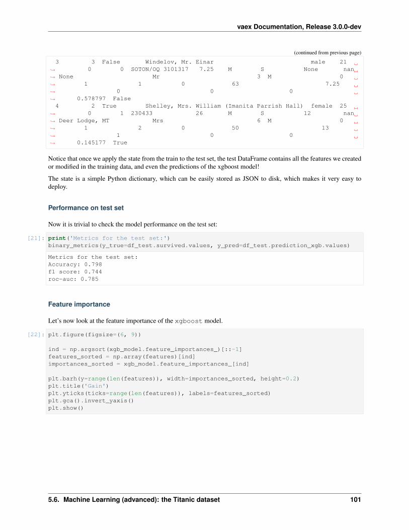
vaex Documentation, Release 3.0.0-dev
(continued from previous page)
3 3 False Windelov, Mr. Einar male 21→˓ 0 0 SOTON/OQ 3101317 7.25 M S None nan→˓ None Mr 3 M 0→˓ 1 1 0 63 7.25→˓ 0 0 0→˓ 0.578797 False4 2 True Shelley, Mrs. William (Imanita Parrish Hall) female 25
→˓ 0 1 230433 26 M S 12 nan→˓ Deer Lodge, MT Mrs 6 M 0→˓ 1 2 0 50 13→˓ 1 0 0→˓ 0.145177 True
Notice that once we apply the state from the train to the test set, the test DataFrame contains all the features we createdor modified in the training data, and even the predictions of the xgboost model!
The state is a simple Python dictionary, which can be easily stored as JSON to disk, which makes it very easy todeploy.
Performance on test set
Now it is trivial to check the model performance on the test set:
[21]: print('Metrics for the test set:')binary_metrics(y_true=df_test.survived.values, y_pred=df_test.prediction_xgb.values)
Metrics for the test set:Accuracy: 0.798f1 score: 0.744roc-auc: 0.785
Feature importance
Let’s now look at the feature importance of the xgboost model.
[22]: plt.figure(figsize=(6, 9))
ind = np.argsort(xgb_model.feature_importances_)[::-1]features_sorted = np.array(features)[ind]importances_sorted = xgb_model.feature_importances_[ind]
plt.barh(y=range(len(features)), width=importances_sorted, height=0.2)plt.title('Gain')plt.yticks(ticks=range(len(features)), labels=features_sorted)plt.gca().invert_yaxis()plt.show()
5.6. Machine Learning (advanced): the Titanic dataset 101
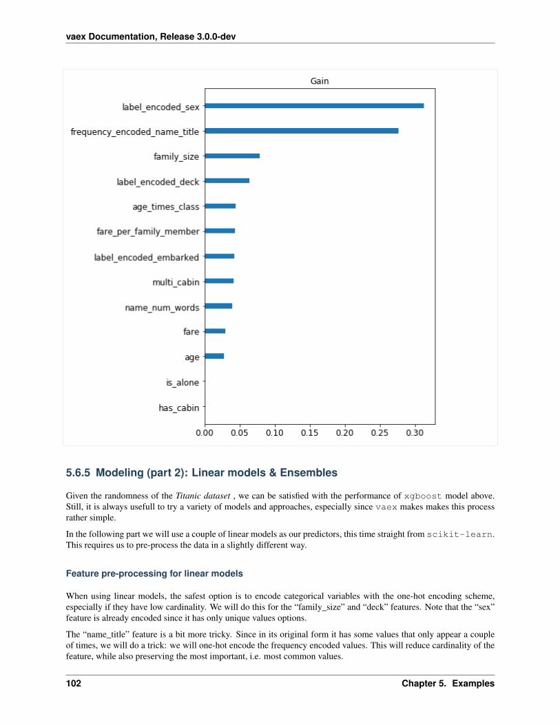
vaex Documentation, Release 3.0.0-dev
5.6.5 Modeling (part 2): Linear models & Ensembles
Given the randomness of the Titanic dataset , we can be satisfied with the performance of xgboost model above.Still, it is always usefull to try a variety of models and approaches, especially since vaex makes makes this processrather simple.
In the following part we will use a couple of linear models as our predictors, this time straight from scikit-learn.This requires us to pre-process the data in a slightly different way.
Feature pre-processing for linear models
When using linear models, the safest option is to encode categorical variables with the one-hot encoding scheme,especially if they have low cardinality. We will do this for the “family_size” and “deck” features. Note that the “sex”feature is already encoded since it has only unique values options.
The “name_title” feature is a bit more tricky. Since in its original form it has some values that only appear a coupleof times, we will do a trick: we will one-hot encode the frequency encoded values. This will reduce cardinality of thefeature, while also preserving the most important, i.e. most common values.
102 Chapter 5. Examples

vaex Documentation, Release 3.0.0-dev
Regarding the “age” and “fare”, to add some variance in the model, we will not convert them to categorical asbefore, but simply remove their mean and standard-deviations (standard-scaling). We will do the same to the“fare_per_family_member” feature.
Finally, we will drop out any other features.
[23]: # One-hot encode categorical featuresone_hot = vaex.ml.OneHotEncoder(features=['deck', 'family_size', 'frequency_encoded_→˓name_title'])df_train = one_hot.fit_transform(df_train)
[24]: # Standard scale numerical featuresstandard_scaler = vaex.ml.StandardScaler(features=['age', 'fare', 'fare_per_family_→˓member'])df_train = standard_scaler.fit_transform(df_train)
[25]: # Get the features for training a linear modelfeatures_linear = df_train.get_column_names(regex='^deck_|^family_size_|^frequency_→˓encoded_name_title_')features_linear += df_train.get_column_names(regex='^standard_scaled_')features_linear += ['label_encoded_sex']features_linear
[25]: ['deck_A','deck_B','deck_C','deck_D','deck_E','deck_F','deck_G','deck_M','family_size_1','family_size_2','family_size_3','family_size_4','family_size_5','family_size_6','family_size_7','family_size_8','family_size_11','frequency_encoded_name_title_0_0009551098376313276','frequency_encoded_name_title_0_0019102196752626551','frequency_encoded_name_title_0_0028653295128939827','frequency_encoded_name_title_0_0057306590257879654','frequency_encoded_name_title_0_007640878701050621','frequency_encoded_name_title_0_045845272206303724','frequency_encoded_name_title_0_1451766953199618','frequency_encoded_name_title_0_20152817574021012','frequency_encoded_name_title_0_5787965616045845','standard_scaled_age','standard_scaled_fare','standard_scaled_fare_per_family_member','label_encoded_sex']
5.6. Machine Learning (advanced): the Titanic dataset 103

vaex Documentation, Release 3.0.0-dev
Estimators: SVC and LogisticRegression
[26]: from sklearn.svm import SVCfrom sklearn.linear_model import LogisticRegression
[27]: # The Support Vector Classifiervaex_svc = vaex.ml.sklearn.Predictor(features=features_linear,
target='survived',model=SVC(max_iter=1000, random_state=42),prediction_name='prediction_svc')
# Logistic Regressionvaex_logistic = vaex.ml.sklearn.Predictor(features=features_linear,
target='survived',model=LogisticRegression(max_iter=1000,
→˓random_state=42),prediction_name='prediction_lr')
# Train the new models and apply the transformation to the train dataframefor model in [vaex_svc, vaex_logistic]:
model.fit(df_train)df_train = model.transform(df_train)
# Preview of the train DataFramedf_train.head(5)
[27]: # pclass survived name sex age sibsp→˓ parch ticket fare cabin embarked boat body home_dest→˓ name_title name_num_words deck multi_cabin has_cabin family_→˓size is_alone age_times_class fare_per_family_member label_encoded_sex→˓ label_encoded_embarked label_encoded_deck frequency_encoded_name_title→˓prediction_xgb deck_A deck_B deck_C deck_D deck_E deck_F→˓deck_G deck_M family_size_1 family_size_2 family_size_3 family_size_→˓4 family_size_5 family_size_6 family_size_7 family_size_8 family_→˓size_11 frequency_encoded_name_title_0_0009551098376313276 frequency_encoded_→˓name_title_0_0019102196752626551 frequency_encoded_name_title_0_→˓0028653295128939827 frequency_encoded_name_title_0_0057306590257879654→˓frequency_encoded_name_title_0_007640878701050621 frequency_encoded_name_title_0_→˓045845272206303724 frequency_encoded_name_title_0_1451766953199618 frequency_→˓encoded_name_title_0_20152817574021012 frequency_encoded_name_title_0_→˓5787965616045845 standard_scaled_age standard_scaled_fare standard_scaled_→˓fare_per_family_member prediction_svc prediction_lr prediction_final0 3 False Stoytcheff, Mr. Ilia male 19 0
→˓ 0 349205 7.8958 M S None nan None→˓ Mr 3 M 0 1→˓1 0 57 7.8958 0→˓ 0 0 0.578797 False→˓ 0 0 0 0 0 0 0→˓ 1 1 0 0 0→˓ 0 0 0 0 0→˓ 0→˓ 0 0→˓ 0→˓ 0 0→˓ 0 0→˓ 1 -0.807704→˓ -0.493719 -0.342804 False False→˓ False
(continues on next page)
104 Chapter 5. Examples

vaex Documentation, Release 3.0.0-dev
(continued from previous page)
1 1 False Payne, Mr. Vivian Ponsonby male 23 0→˓ 0 12749 93.5 B24 S None nan Montreal, PQ→˓ Mr 4 B 0 1→˓1 0 23 93.5 0→˓ 0 1 0.578797 False→˓ 0 1 0 0 0 0 0→˓ 0 1 0 0 0→˓ 0 0 0 0 0→˓ 0→˓ 0 0→˓ 0→˓ 0 0→˓ 0 0→˓ 1 -0.492921→˓ 1.19613 1.99718 False True→˓ False2 3 True Abbott, Mrs. Stanton (Rosa Hunt) female 35 1
→˓ 1 C.A. 2673 20.25 M S A nan East Providence,→˓RI Mrs 5 M 0 1→˓ 3 0 105 6.75 1→˓ 0 0 0.145177 True→˓ 0 0 0 0 0 0 0→˓ 1 0 0 1 0→˓ 0 0 0 0 0→˓ 0→˓ 0 0→˓ 0→˓ 0 0→˓ 1 0→˓ 0 0.45143→˓ -0.249845 -0.374124 True True→˓ True3 2 True Hocking, Miss. Ellen "Nellie" female 20 2
→˓ 1 29105 23 M S 4 nan Cornwall / Akron,→˓OH Miss 4 M 0 1→˓4 0 40 5.75 1→˓ 0 0 0.201528 True→˓ 0 0 0 0 0 0 0→˓ 1 0 0 0 1→˓ 0 0 0 0 0→˓ 0→˓ 0 0→˓ 0→˓ 0 0→˓ 0 1→˓ 0 -0.729008→˓ -0.195559 -0.401459 True True→˓ True4 3 False Nilsson, Mr. August Ferdinand male 21 0
→˓ 0 350410 7.8542 M S None nan None→˓ Mr 4 M 0 1→˓1 0 63 7.8542 0→˓ 0 0 0.578797 False→˓ 0 0 0 0 0 0 0→˓ 1 1 0 0 0→˓ 0 0 0 0 0→˓ 0→˓ 0 0→˓ 0→˓ 0 0→˓ 0 0→˓ 1 -0.650312→˓ -0.494541 -0.343941 False False→˓ False
(continues on next page)
5.6. Machine Learning (advanced): the Titanic dataset 105

vaex Documentation, Release 3.0.0-dev
(continued from previous page)
Ensemble
Just as before, the predictions from the SVC and the LogisticRegression classifiers are added as virtual columnsin the training dataset. This is quite powerful, since now we can easily use them to create an ensemble! For example,let’s do a weighted mean.
[28]: # Weighed mean of the classesprediction_final = (df_train.prediction_xgb.astype('int') * 0.3 +
df_train.prediction_svc.astype('int') * 0.5 +df_train.prediction_xgb.astype('int') * 0.2)
# Get the predicted classprediction_final = (prediction_final >= 0.5)# Add the expression to the train DataFramedf_train['prediction_final'] = prediction_final
# Previewdf_train[df_train.get_column_names(regex='^predict')]
[28]: # prediction_xgb prediction_svc prediction_lr prediction_final0 False False False False1 False False True False2 True True True True3 True True True True4 False False False False... ... ... ... ...1,042 False False False False1,043 False True True True1,044 True True True True1,045 False False True False1,046 False False False False
Performance (part 2)
Applying the ensembler to the test set is just as easy as before. We just need to get the new state of the trainingDataFrame, and transfer it to the test DataFrame.
[29]: # State transferstate_new = df_train.state_get()df_test.state_set(state_new)
# Previewdf_test.head(5)
106 Chapter 5. Examples

vaex Documentation, Release 3.0.0-dev
[29]: # pclass survived name sex→˓age sibsp parch ticket fare cabin embarked boat→˓body home_dest name_title name_num_words deck multi_→˓cabin has_cabin family_size is_alone age_times_class fare_per_family_→˓member label_encoded_sex label_encoded_embarked label_encoded_deck→˓frequency_encoded_name_title prediction_xgb deck_A deck_B deck_C→˓deck_D deck_E deck_F deck_G deck_M family_size_1 family_size_2→˓family_size_3 family_size_4 family_size_5 family_size_6 family_size_7→˓ family_size_8 family_size_11 frequency_encoded_name_title_0_→˓0009551098376313276 frequency_encoded_name_title_0_0019102196752626551→˓frequency_encoded_name_title_0_0028653295128939827 frequency_encoded_name_title_→˓0_0057306590257879654 frequency_encoded_name_title_0_007640878701050621→˓frequency_encoded_name_title_0_045845272206303724 frequency_encoded_name_title_0_→˓1451766953199618 frequency_encoded_name_title_0_20152817574021012 frequency_→˓encoded_name_title_0_5787965616045845 standard_scaled_age standard_scaled_→˓fare standard_scaled_fare_per_family_member prediction_svc prediction_lr→˓prediction_final0 3 False O'Connor, Mr. Patrick male 28.
→˓032 0 0 366713 7.75 M Q None→˓nan None Mr 3 M→˓0 1 1 0 84.096 7.→˓75 0 1 0→˓ 0.578797 False 0 0 0 0→˓ 0 0 0 1 1 0→˓ 0 0 0 0 0→˓ 0 0 0→˓ 0→˓ 0 0→˓ 0→˓ 0 0→˓ 0 1→˓ -0.096924 -0.496597 -0.346789→˓False False False1 3 False Canavan, Mr. Patrick male 21
→˓ 0 0 364858 7.75 M Q None nan→˓ Ireland Philadelphia, PA Mr 3 M 0→˓ 1 1 0 63 7.75→˓ 0 1 0→˓ 0.578797 False 0 0 0 0 0→˓ 0 0 1 1 0 0→˓ 0 0 0 0 0→˓ 0 0→˓ 0→˓ 0 0→˓ 0→˓0 0→˓ 0 1→˓-0.650312 -0.496597 -0.346789 False→˓ False False2 1 False Ovies y Rodriguez, Mr. Servando male 28.5
→˓ 0 0 PC 17562 27.7208 D43 C None 189→˓ ?Havana, Cuba Mr 5 D 0→˓ 1 1 0 28.5 27.7208→˓ 0 2 4→˓ 0.578797 True 0 0 0 1 0→˓ 0 0 0 1 0 0→˓ 0 0 0 0 0→˓ 0 0→˓ 0→˓ 0 0→˓ 0→˓0 0→˓ 0 1→˓-0.0600935 -0.102369 0.19911 False→˓ False True
(continues on next page)
5.6. Machine Learning (advanced): the Titanic dataset 107

vaex Documentation, Release 3.0.0-dev
(continued from previous page)
3 3 False Windelov, Mr. Einar male 21→˓ 0 0 SOTON/OQ 3101317 7.25 M S None nan→˓ None Mr 3 M 0→˓ 1 1 0 63 7.25→˓ 0 0 0→˓ 0.578797 False 0 0 0 0 0→˓ 0 0 1 1 0 0→˓ 0 0 0 0 0→˓ 0 0→˓ 0→˓ 0 0→˓ 0→˓0 0→˓ 0 1→˓-0.650312 -0.506468 -0.360456 False→˓ False False4 2 True Shelley, Mrs. William (Imanita Parrish Hall) female 25
→˓ 0 1 230433 26 M S 12 nan→˓ Deer Lodge, MT Mrs 6 M 0→˓ 1 2 0 50 13→˓ 1 0 0→˓ 0.145177 True 0 0 0 0 0→˓ 0 0 1 0 1 0→˓ 0 0 0 0 0→˓ 0 0→˓ 0→˓ 0 0→˓ 0→˓0 1→˓ 0 0→˓-0.335529 -0.136338 -0.203281 True→˓ True True
Finally, let’s check the performance of all the individual models as well as on the ensembler, on the test set.
[30]: pred_columns = df_train.get_column_names(regex='^prediction_')for i in pred_columns:
print(i)binary_metrics(y_true=df_test.survived.values, y_pred=df_test[i].values)print(' ')
prediction_xgbAccuracy: 0.798f1 score: 0.744roc-auc: 0.785
prediction_svcAccuracy: 0.813f1 score: 0.763roc-auc: 0.801
prediction_lrAccuracy: 0.794f1 score: 0.743roc-auc: 0.783
prediction_final
(continues on next page)
108 Chapter 5. Examples

vaex Documentation, Release 3.0.0-dev
(continued from previous page)
Accuracy: 0.832f1 score: 0.802roc-auc: 0.831
We see that our ensembler is doing a better job than any idividual model, as expected.
Thanks you for going over this example. Feel free to copy, modify, and in general play around with this notebook.
5.6. Machine Learning (advanced): the Titanic dataset 109

vaex Documentation, Release 3.0.0-dev
110 Chapter 5. Examples

CHAPTER 6
API documentation for vaex library
6.1 Quick lists
6.1.1 Opening/reading in your data.
vaex.open(path[, convert, shuffle, copy_index]) Open a DataFrame from file given by path.vaex.from_arrow_table(table) Creates a vaex DataFrame from an arrow Table.vaex.from_arrays(**arrays) Create an in memory DataFrame from numpy arrays.vaex.from_dict(data) Create an in memory dataset from a dict with column
names as keys and list/numpy-arrays as valuesvaex.from_csv(filename_or_buffer[, . . . ]) Read a CSV file as a DataFrame, and optionally convert
to an hdf5 file.vaex.from_ascii(path[, seperator, names, . . . ]) Create an in memory DataFrame from an ascii file
(whitespace seperated by default).vaex.from_pandas(df[, name, copy_index, . . . ]) Create an in memory DataFrame from a pandas
DataFrame.vaex.from_astropy_table(table) Create a vaex DataFrame from an Astropy Table.
6.1.2 Visualization.
vaex.dataframe.DataFrame.plot([x, y, z,. . . ])
Viz data in a 2d histogram/heatmap.
vaex.dataframe.DataFrame.plot1d([x,what, . . . ])
Viz data in 1d (histograms, running means etc)
vaex.dataframe.DataFrame.scatter(x, y[,. . . ])
Viz (small amounts) of data in 2d using a scatter plot
vaex.dataframe.DataFrame.plot_widget(x, y[, . . . ])
Viz 1d, 2d or 3d in a Jupyter notebook
Continued on next page
111

vaex Documentation, Release 3.0.0-dev
Table 2 – continued from previous pagevaex.dataframe.DataFrame.healpix_plot([. . . ])
Viz data in 2d using a healpix column.
6.1.3 Statistics.
vaex.dataframe.DataFrame.count([expression, . . . ])
Count the number of non-NaN values (or all, if expres-sion is None or “*”).
vaex.dataframe.DataFrame.mean(expression[, . . . ])
Calculate the mean for expression, possibly on a griddefined by binby.
vaex.dataframe.DataFrame.std(expression[,. . . ])
Calculate the standard deviation for the given expres-sion, possible on a grid defined by binby
vaex.dataframe.DataFrame.var(expression[,. . . ])
Calculate the sample variance for the given expression,possible on a grid defined by binby
vaex.dataframe.DataFrame.cov(x[, y, binby,. . . ])
Calculate the covariance matrix for x and y or more ex-pressions, possibly on a grid defined by binby.
vaex.dataframe.DataFrame.correlation(x[, y, . . . ])
Calculate the correlation coefficientcov[x,y]/(std[x]*std[y]) between x and y, possiblyon a grid defined by binby.
vaex.dataframe.DataFrame.median_approx(. . . )
Calculate the median, possibly on a grid defined bybinby.
vaex.dataframe.DataFrame.mode(expression[, . . . ])
Calculate/estimate the mode.
vaex.dataframe.DataFrame.min(expression[,. . . ])
Calculate the minimum for given expressions, possiblyon a grid defined by binby.
vaex.dataframe.DataFrame.max(expression[,. . . ])
Calculate the maximum for given expressions, possiblyon a grid defined by binby.
vaex.dataframe.DataFrame.minmax(expression)
Calculate the minimum and maximum for expressions,possibly on a grid defined by binby.
vaex.dataframe.DataFrame.mutual_information(x)
Estimate the mutual information between and x and yon a grid with shape mi_shape and mi_limits, possiblyon a grid defined by binby.
6.2 vaex-core
Vaex is a library for dealing with larger than memory DataFrames (out of core).
The most important class (datastructure) in vaex is the DataFrame. A DataFrame is obtained by either opening theexample dataset:
>>> import vaex>>> df = vaex.example()
Or using open() to open a file.
>>> df1 = vaex.open("somedata.hdf5")>>> df2 = vaex.open("somedata.fits")>>> df2 = vaex.open("somedata.arrow")>>> df4 = vaex.open("somedata.csv")
Or connecting to a remove server:
112 Chapter 6. API documentation for vaex library

vaex Documentation, Release 3.0.0-dev
>>> df_remote = vaex.open("http://try.vaex.io/nyc_taxi_2015")
A few strong features of vaex are:
• Performance: works with huge tabular data, process over a billion (> 109) rows/second.
• Expression system / Virtual columns: compute on the fly, without wasting ram.
• Memory efficient: no memory copies when doing filtering/selections/subsets.
• Visualization: directly supported, a one-liner is often enough.
• User friendly API: you will only need to deal with a DataFrame object, and tab completion + docstring will helpyou out: ds.mean<tab>, feels very similar to Pandas.
• Very fast statistics on N dimensional grids such as histograms, running mean, heatmaps.
Follow the tutorial at https://docs.vaex.io/en/latest/tutorial.html to learn how to use vaex.
vaex.open(path, convert=False, shuffle=False, copy_index=True, *args, **kwargs)Open a DataFrame from file given by path.
Example:
>>> df = vaex.open('sometable.hdf5')>>> df = vaex.open('somedata*.csv', convert='bigdata.hdf5')
Parameters
• or list path (str) – local or absolute path to file, or glob string, or list of paths
• convert – convert files to an hdf5 file for optimization, can also be a path
• shuffle (bool) – shuffle converted DataFrame or not
• args – extra arguments for file readers that need it
• kwargs – extra keyword arguments
• copy_index (bool) – copy index when source is read via pandas
Returns return a DataFrame on success, otherwise None
Return type DataFrame
S3 support:
Vaex supports streaming in hdf5 files from Amazon AWS object storage S3. Files are by default cached in$HOME/.vaex/file-cache/s3 such that successive access is as fast as native disk access. The following url pa-rameters control S3 options:
• anon: Use anonymous access or not (false by default). (Allowed values are: true,True,1,false,False,0)
• use_cache: Use the disk cache or not, only set to false if the data should be accessed once. (Allowed valuesare: true,True,1,false,False,0)
• profile_name and other arguments are passed to s3fs.core.S3FileSystem
All arguments can also be passed as kwargs, but then arguments such as anon can only be a boolean, not a string.
Examples:
6.2. vaex-core 113
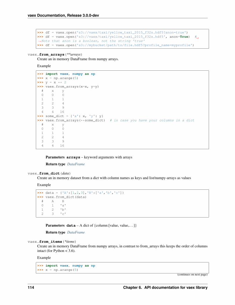
vaex Documentation, Release 3.0.0-dev
>>> df = vaex.open('s3://vaex/taxi/yellow_taxi_2015_f32s.hdf5?anon=true')>>> df = vaex.open('s3://vaex/taxi/yellow_taxi_2015_f32s.hdf5', anon=True) #→˓Note that anon is a boolean, not the string 'true'>>> df = vaex.open('s3://mybucket/path/to/file.hdf5?profile_name=myprofile')
vaex.from_arrays(**arrays)Create an in memory DataFrame from numpy arrays.
Example
>>> import vaex, numpy as np>>> x = np.arange(5)>>> y = x ** 2>>> vaex.from_arrays(x=x, y=y)# x y0 0 01 1 12 2 43 3 94 4 16
>>> some_dict = {'x': x, 'y': y}>>> vaex.from_arrays(**some_dict) # in case you have your columns in a dict# x y0 0 01 1 12 2 43 3 94 4 16
Parameters arrays – keyword arguments with arrays
Return type DataFrame
vaex.from_dict(data)Create an in memory dataset from a dict with column names as keys and list/numpy-arrays as values
Example
>>> data = {'A':[1,2,3],'B':['a','b','c']}>>> vaex.from_dict(data)# A B0 1 'a'1 2 'b'2 3 'c'
Parameters data – A dict of {column:[value, value,. . . ]}
Return type DataFrame
vaex.from_items(*items)Create an in memory DataFrame from numpy arrays, in contrast to from_arrays this keeps the order of columnsintact (for Python < 3.6).
Example
>>> import vaex, numpy as np>>> x = np.arange(5)
(continues on next page)
114 Chapter 6. API documentation for vaex library

vaex Documentation, Release 3.0.0-dev
(continued from previous page)
>>> y = x ** 2>>> vaex.from_items(('x', x), ('y', y))# x y0 0 01 1 12 2 43 3 94 4 16
Parameters items – list of [(name, numpy array), . . . ]
Return type DataFrame
vaex.from_arrow_table(table)Creates a vaex DataFrame from an arrow Table.
Return type DataFrame
vaex.from_csv(filename_or_buffer, copy_index=True, chunk_size=None, convert=False, **kwargs)Read a CSV file as a DataFrame, and optionally convert to an hdf5 file.
Parameters
• or file filename_or_buffer (str) – CSV file path or file-like
• copy_index (bool) – copy index when source is read via Pandas
• chunk_size (int) – if the CSV file is too big to fit in the memory this parameter can beused to read CSV file in chunks. For example:
>>> import vaex>>> for i, df in enumerate(vaex.from_csv('taxi.csv', chunk_→˓size=100_000)):>>> df = df[df.passenger_count < 6]>>> df.export_hdf5(f'taxi_{i:02}.hdf5')
• or str convert (bool) – convert files to an hdf5 file for optimization, can also be apath. The CSV file will be read in chunks: either using the provided chunk_size argument,or a default size. Each chunk will be saved as a separate hdf5 file, then all of them will becombined into one hdf5 file. So for a big CSV file you will need at least double of extraspace on the disk. Default chunk_size for converting is 5 million rows, which correspondsto around 1Gb memory on an example of NYC Taxi dataset.
• kwargs – extra keyword arguments, currently passed to Pandas read_csv function, but theimplementation might change in future versions.
Returns DataFrame
vaex.from_ascii(path, seperator=None, names=True, skip_lines=0, skip_after=0, **kwargs)Create an in memory DataFrame from an ascii file (whitespace seperated by default).
>>> ds = vx.from_ascii("table.asc")>>> ds = vx.from_ascii("table.csv", seperator=",", names=["x", "y", "z"])
Parameters
• path – file path
• seperator – value seperator, by default whitespace, use “,” for comma seperated values.
6.2. vaex-core 115

vaex Documentation, Release 3.0.0-dev
• names – If True, the first line is used for the column names, otherwise provide a list ofstrings with names
• skip_lines – skip lines at the start of the file
• skip_after – skip lines at the end of the file
• kwargs –
Return type DataFrame
vaex.from_pandas(df, name=’pandas’, copy_index=True, index_name=’index’)Create an in memory DataFrame from a pandas DataFrame.
Param pandas.DataFrame df: Pandas DataFrame
Param name: unique for the DataFrame
>>> import vaex, pandas as pd>>> df_pandas = pd.from_csv('test.csv')>>> df = vaex.from_pandas(df_pandas)
Return type DataFrame
vaex.from_astropy_table(table)Create a vaex DataFrame from an Astropy Table.
vaex.from_samp(username=None, password=None)Connect to a SAMP Hub and wait for a single table load event, disconnect, download the table and return theDataFrame.
Useful if you want to send a single table from say TOPCAT to vaex in a python console or notebook.
vaex.open_many(filenames)Open a list of filenames, and return a DataFrame with all DataFrames concatenated.
Parameters filenames (list[str]) – list of filenames/paths
Return type DataFrame
vaex.register_function(scope=None, as_property=False, name=None, on_expression=True,df_accessor=None)
Decorator to register a new function with vaex.
If on_expression is True, the function will be available as a method on an Expression, where the first argumentwill be the expression itself.
If df_accessor is given, it is added as a method to that dataframe accessor (see e.g. vaex/geo.py)
Example:
>>> import vaex>>> df = vaex.example()>>> @vaex.register_function()>>> def invert(x):>>> return 1/x>>> df.x.invert()
>>> import numpy as np>>> df = vaex.from_arrays(departure=np.arange('2015-01-01', '2015-12-05', dtype=→˓'datetime64'))
(continues on next page)
116 Chapter 6. API documentation for vaex library
vaex Documentation, Release 3.0.0-dev
(continued from previous page)
>>> @vaex.register_function(as_property=True, scope='dt')>>> def dt_relative_day(x):>>> return vaex.functions.dt_dayofyear(x)/365.>>> df.departure.dt.relative_day
vaex.example()Returns an example DataFrame which comes with vaex for testing/learning purposes.
Return type DataFrame
vaex.app(*args, **kwargs)Create a vaex app, the QApplication mainloop must be started.
In ipython notebook/jupyter do the following:
>>> import vaex.ui.main # this causes the qt api level to be set properly>>> import vaex
Next cell:
>>> %gui qt
Next cell:
>>> app = vaex.app()
From now on, you can run the app along with jupyter
vaex.delayed(f)Decorator to transparantly accept delayed computation.
Example:
>>> delayed_sum = ds.sum(ds.E, binby=ds.x, limits=limits,>>> shape=4, delay=True)>>> @vaex.delayed>>> def total_sum(sums):>>> return sums.sum()>>> sum_of_sums = total_sum(delayed_sum)>>> ds.execute()>>> sum_of_sums.get()See the tutorial for a more complete example https://docs.vaex.io/en/latest/→˓tutorial.html#Parallel-computations
6.2.1 DataFrame class
class vaex.dataframe.DataFrame(name, column_names, executor=None)Bases: object
All local or remote datasets are encapsulated in this class, which provides a pandas like API to your dataset.
Each DataFrame (df) has a number of columns, and a number of rows, the length of the DataFrame.
All DataFrames have multiple ‘selection’, and all calculations are done on the whole DataFrame (default) or forthe selection. The following example shows how to use the selection.
6.2. vaex-core 117

vaex Documentation, Release 3.0.0-dev
>>> df.select("x < 0")>>> df.sum(df.y, selection=True)>>> df.sum(df.y, selection=[df.x < 0, df.x > 0])
__delitem__(item)Removes a (virtual) column from the DataFrame.
Note: this does not check if the column is used in a virtual expression or in the filter and may lead to issues.It is safer to use drop().
__getitem__(item)Convenient way to get expressions, (shallow) copies of a few columns, or to apply filtering.
Example:
>>> df['Lz'] # the expression 'Lz>>> df['Lz/2'] # the expression 'Lz/2'>>> df[["Lz", "E"]] # a shallow copy with just two columns>>> df[df.Lz < 0] # a shallow copy with the filter Lz < 0 applied
__init__(name, column_names, executor=None)Initialize self. See help(type(self)) for accurate signature.
__iter__()Iterator over the column names.
__len__()Returns the number of rows in the DataFrame (filtering applied).
__repr__()Return repr(self).
__setitem__(name, value)Convenient way to add a virtual column / expression to this DataFrame.
Example:
>>> import vaex, numpy as np>>> df = vaex.example()>>> df['r'] = np.sqrt(df.x**2 + df.y**2 + df.z**2)>>> df.r<vaex.expression.Expression(expressions='r')> instance at 0x121687e80→˓values=[2.9655450396553587, 5.77829281049018, 6.99079603950256, 9.→˓431842752707537, 0.8825613121347967 ... (total 330000 values) ... 7.→˓453831761514681, 15.398412491068198, 8.864250273925633, 17.601047186042507,→˓14.540181524970293]
__str__()Return str(self).
__weakref__list of weak references to the object (if defined)
add_column(name, f_or_array, dtype=None)Add an in memory array as a column.
add_variable(name, expression, overwrite=True, unique=True)Add a variable to a DataFrame.
118 Chapter 6. API documentation for vaex library

vaex Documentation, Release 3.0.0-dev
A variable may refer to other variables, and virtual columns and expression may refer to variables.
Example
>>> df.add_variable('center', 0)>>> df.add_virtual_column('x_prime', 'x-center')>>> df.select('x_prime < 0')
Param str name: name of virtual varible
Param expression: expression for the variable
add_virtual_column(name, expression, unique=False)Add a virtual column to the DataFrame.
Example:
>>> df.add_virtual_column("r", "sqrt(x**2 + y**2 + z**2)")>>> df.select("r < 10")
Param str name: name of virtual column
Param expression: expression for the column
Parameters unique (str) – if name is already used, make it unique by adding a postfix, e.g._1, or _2
apply(f, arguments=None, dtype=None, delay=False, vectorize=False)Apply a function on a per row basis across the entire DataFrame.
Example:
>>> import vaex>>> df = vaex.example()>>> def func(x, y):... return (x+y)/(x-y)...>>> df.apply(func, arguments=[df.x, df.y])Expression = lambda_function(x, y)Length: 330,000 dtype: float64 (expression)-------------------------------------------
0 -0.4607891 3.900382 -0.6428513 0.6857684 -0.543357
Parameters
• f – The function to be applied
• arguments – List of arguments to be passed on to the function f.
Returns A function that is lazily evaluated.
byte_size(selection=False, virtual=False)Return the size in bytes the whole DataFrame requires (or the selection), respecting the active_fraction.
6.2. vaex-core 119

vaex Documentation, Release 3.0.0-dev
cat(i1, i2, format=’html’)Display the DataFrame from row i1 till i2
For format, see https://pypi.org/project/tabulate/
Parameters
• i1 (int) – Start row
• i2 (int) – End row.
• format (str) – Format to use, e.g. ‘html’, ‘plain’, ‘latex’
close_files()Close any possible open file handles, the DataFrame will not be in a usable state afterwards.
colGives direct access to the columns only (useful for tab completion).
Convenient when working with ipython in combination with small DataFrames, since this gives tab-completion.
Columns can be accessed by their names, which are attributes. The attributes are currently expressions, soyou can do computations with them.
Example
>>> ds = vaex.example()>>> df.plot(df.col.x, df.col.y)
column_count(hidden=False)Returns the number of columns (including virtual columns).
Parameters hidden (bool) – If True, include hidden columns in the tally
Returns Number of columns in the DataFrame
combinations(expressions_list=None, dimension=2, exclude=None, **kwargs)Generate a list of combinations for the possible expressions for the given dimension.
Parameters
• expressions_list – list of list of expressions, where the inner list defines the sub-space
• dimensions – if given, generates a subspace with all possible combinations for thatdimension
• exclude – list of
correlation(x, y=None, binby=[], limits=None, shape=128, sort=False, sort_key=<ufunc ’abso-lute’>, selection=False, delay=False, progress=None)
Calculate the correlation coefficient cov[x,y]/(std[x]*std[y]) between x and y, possibly on a grid definedby binby.
Example:
>>> df.correlation("x**2+y**2+z**2", "-log(-E+1)")array(0.6366637382215669)>>> df.correlation("x**2+y**2+z**2", "-log(-E+1)", binby="Lz", shape=4)array([ 0.40594394, 0.69868851, 0.61394099, 0.65266318])
Parameters
120 Chapter 6. API documentation for vaex library

vaex Documentation, Release 3.0.0-dev
• x – expression or list of expressions, e.g. df.x, ‘x’, or [‘x, ‘y’]
• y – expression or list of expressions, e.g. df.x, ‘x’, or [‘x, ‘y’]
• binby – List of expressions for constructing a binned grid
• limits – description for the min and max values for the expressions, e.g. ‘minmax’(default), ‘99.7%’, [0, 10], or a list of, e.g. [[0, 10], [0, 20], ‘minmax’]
• shape – shape for the array where the statistic is calculated on, if only an integer is given,it is used for all dimensions, e.g. shape=128, shape=[128, 256]
• selection – Name of selection to use (or True for the ‘default’), or all the data (whenselection is None or False), or a list of selections
• delay – Do not return the result, but a proxy for delayhronous calculations (currentlyonly for internal use)
• progress – A callable that takes one argument (a floating point value between 0 and 1)indicating the progress, calculations are cancelled when this callable returns False
Returns Numpy array with the given shape, or a scalar when no binby argument is given, withthe statistic
count(expression=None, binby=[], limits=None, shape=128, selection=False, delay=False,edges=False, progress=None, array_type=None)
Count the number of non-NaN values (or all, if expression is None or “*”).
Example:
>>> df.count()330000>>> df.count("*")330000.0>>> df.count("*", binby=["x"], shape=4)array([ 10925., 155427., 152007., 10748.])
Parameters
• expression – Expression or column for which to count non-missing values, or Noneor ‘*’ for counting the rows
• binby – List of expressions for constructing a binned grid
• limits – description for the min and max values for the expressions, e.g. ‘minmax’(default), ‘99.7%’, [0, 10], or a list of, e.g. [[0, 10], [0, 20], ‘minmax’]
• shape – shape for the array where the statistic is calculated on, if only an integer is given,it is used for all dimensions, e.g. shape=128, shape=[128, 256]
• selection – Name of selection to use (or True for the ‘default’), or all the data (whenselection is None or False), or a list of selections
• delay – Do not return the result, but a proxy for delayhronous calculations (currentlyonly for internal use)
• progress – A callable that takes one argument (a floating point value between 0 and 1)indicating the progress, calculations are cancelled when this callable returns False
• edges – Currently for internal use only (it includes nan’s and values outside the limits atborders, nan and 0, smaller than at 1, and larger at -1
6.2. vaex-core 121

vaex Documentation, Release 3.0.0-dev
• array_type – Type of output array, possible values are None/”numpy” (ndarray), “xar-ray” for a xarray.DataArray, or “list” for a Python list
Returns Numpy array with the given shape, or a scalar when no binby argument is given, withthe statistic
cov(x, y=None, binby=[], limits=None, shape=128, selection=False, delay=False, progress=None)Calculate the covariance matrix for x and y or more expressions, possibly on a grid defined by binby.
Either x and y are expressions, e.g.:
>>> df.cov("x", "y")
Or only the x argument is given with a list of expressions, e.g.:
>>> df.cov(["x, "y, "z"])
Example:
>>> df.cov("x", "y")array([[ 53.54521742, -3.8123135 ],[ -3.8123135 , 60.62257881]])>>> df.cov(["x", "y", "z"])array([[ 53.54521742, -3.8123135 , -0.98260511],[ -3.8123135 , 60.62257881, 1.21381057],[ -0.98260511, 1.21381057, 25.55517638]])
>>> df.cov("x", "y", binby="E", shape=2)array([[[ 9.74852878e+00, -3.02004780e-02],[ -3.02004780e-02, 9.99288215e+00]],[[ 8.43996546e+01, -6.51984181e+00],[ -6.51984181e+00, 9.68938284e+01]]])
Parameters
• x – expression or list of expressions, e.g. df.x, ‘x’, or [‘x, ‘y’]
• y – if previous argument is not a list, this argument should be given
• binby – List of expressions for constructing a binned grid
• limits – description for the min and max values for the expressions, e.g. ‘minmax’(default), ‘99.7%’, [0, 10], or a list of, e.g. [[0, 10], [0, 20], ‘minmax’]
• shape – shape for the array where the statistic is calculated on, if only an integer is given,it is used for all dimensions, e.g. shape=128, shape=[128, 256]
• selection – Name of selection to use (or True for the ‘default’), or all the data (whenselection is None or False), or a list of selections
• delay – Do not return the result, but a proxy for delayhronous calculations (currentlyonly for internal use)
Returns Numpy array with the given shape, or a scalar when no binby argument is given, withthe statistic, the last dimensions are of shape (2,2)
covar(x, y, binby=[], limits=None, shape=128, selection=False, delay=False, progress=None)Calculate the covariance cov[x,y] between x and y, possibly on a grid defined by binby.
Example:
122 Chapter 6. API documentation for vaex library

vaex Documentation, Release 3.0.0-dev
>>> df.covar("x**2+y**2+z**2", "-log(-E+1)")array(52.69461456005138)>>> df.covar("x**2+y**2+z**2", "-log(-E+1)")/(df.std("x**2+y**2+z**2") * df.→˓std("-log(-E+1)"))0.63666373822156686>>> df.covar("x**2+y**2+z**2", "-log(-E+1)", binby="Lz", shape=4)array([ 10.17387143, 51.94954078, 51.24902796, 20.2163929 ])
Parameters
• x – expression or list of expressions, e.g. df.x, ‘x’, or [‘x, ‘y’]
• y – expression or list of expressions, e.g. df.x, ‘x’, or [‘x, ‘y’]
• binby – List of expressions for constructing a binned grid
• limits – description for the min and max values for the expressions, e.g. ‘minmax’(default), ‘99.7%’, [0, 10], or a list of, e.g. [[0, 10], [0, 20], ‘minmax’]
• shape – shape for the array where the statistic is calculated on, if only an integer is given,it is used for all dimensions, e.g. shape=128, shape=[128, 256]
• selection – Name of selection to use (or True for the ‘default’), or all the data (whenselection is None or False), or a list of selections
• delay – Do not return the result, but a proxy for delayhronous calculations (currentlyonly for internal use)
• progress – A callable that takes one argument (a floating point value between 0 and 1)indicating the progress, calculations are cancelled when this callable returns False
Returns Numpy array with the given shape, or a scalar when no binby argument is given, withthe statistic
data_type(expression, internal=False)Return the numpy dtype for the given expression, if not a column, the first row will be evaluated to get thedtype.
delete_variable(name)Deletes a variable from a DataFrame.
delete_virtual_column(name)Deletes a virtual column from a DataFrame.
describe(strings=True, virtual=True, selection=None)Give a description of the DataFrame.
>>> import vaex>>> df = vaex.example()[['x', 'y', 'z']]>>> df.describe()
x y zdtype float64 float64 float64count 330000 330000 330000missing 0 0 0mean -0.0671315 -0.0535899 0.0169582std 7.31746 7.78605 5.05521min -128.294 -71.5524 -44.3342max 271.366 146.466 50.7185>>> df.describe(selection=df.x > 0)
x y z
(continues on next page)
6.2. vaex-core 123

vaex Documentation, Release 3.0.0-dev
(continued from previous page)
dtype float64 float64 float64count 164060 164060 164060missing 165940 165940 165940mean 5.13572 -0.486786 -0.0868073std 5.18701 7.61621 5.02831min 1.51635e-05 -71.5524 -44.3342max 271.366 78.0724 40.2191
Parameters
• strings (bool) – Describe string columns or not
• virtual (bool) – Describe virtual columns or not
• selection – Optional selection to use.
Returns Pandas dataframe
drop(columns, inplace=False, check=True)Drop columns (or a single column).
Parameters
• columns – List of columns or a single column name
• inplace – Make modifications to self or return a new DataFrame
• check – When true, it will check if the column is used in virtual columns or the filter,and hide it instead.
drop_filter(inplace=False)Removes all filters from the DataFrame
dropmissing(column_names=None)Create a shallow copy of a DataFrame, with filtering set using ismissing.
Parameters column_names – The columns to consider, default: all (real, non-virtual)columns
Return type DataFrame
dropna(column_names=None)Create a shallow copy of a DataFrame, with filtering set using isna.
Parameters column_names – The columns to consider, default: all (real, non-virtual)columns
Return type DataFrame
dropnan(column_names=None)Create a shallow copy of a DataFrame, with filtering set using isnan.
Parameters column_names – The columns to consider, default: all (real, non-virtual)columns
Return type DataFrame
dtypesGives a Pandas series object containing all numpy dtypes of all columns (except hidden).
evaluate(expression, i1=None, i2=None, out=None, selection=None, filtered=True, internal=None,parallel=True, chunk_size=None)
Evaluate an expression, and return a numpy array with the results for the full column or a part of it.
124 Chapter 6. API documentation for vaex library

vaex Documentation, Release 3.0.0-dev
Note that this is not how vaex should be used, since it means a copy of the data needs to fit in memory.
To get partial results, use i1 and i2
Parameters
• expression (str) – Name/expression to evaluate
• i1 (int) – Start row index, default is the start (0)
• i2 (int) – End row index, default is the length of the DataFrame
• out (ndarray) – Output array, to which the result may be written (may be used to reusean array, or write to a memory mapped array)
• selection – selection to apply
Returns
evaluate_iterator(expression, s1=None, s2=None, out=None, selection=None, filtered=True, in-ternal=None, parallel=True, chunk_size=None, prefetch=True)
Generator to efficiently evaluate expressions in chunks (number of rows).
See DataFrame.evaluate() for other arguments.
Example:
>>> import vaex>>> df = vaex.example()>>> for i1, i2, chunk in df.evaluate_iterator(df.x, chunk_size=100_000):... print(f"Total of {i1} to {i2} = {chunk.sum()}")...Total of 0 to 100000 = -7460.610158279056Total of 100000 to 200000 = -4964.85827154921Total of 200000 to 300000 = -7303.271340043915Total of 300000 to 330000 = -2424.65234724951
Parameters prefetch – Prefetch/compute the next chunk in parallel while the current valueis yielded/returned.
evaluate_variable(name)Evaluates the variable given by name.
execute()Execute all delayed jobs.
extract()Return a DataFrame containing only the filtered rows.
Note: Note that no copy of the underlying data is made, only a view/reference is made.
The resulting DataFrame may be more efficient to work with when the original DataFrame is heavilyfiltered (contains just a small number of rows).
If no filtering is applied, it returns a trimmed view. For the returned df, len(df) == df.length_original() ==df.length_unfiltered()
Return type DataFrame
fillna(value, column_names=None, prefix=’__original_’, inplace=False)Return a DataFrame, where missing values/NaN are filled with ‘value’.
6.2. vaex-core 125
vaex Documentation, Release 3.0.0-dev
The original columns will be renamed, and by default they will be hidden columns. No data is lost.
Note: Note that no copy of the underlying data is made, only a view/reference is made.
Note: Note that filtering will be ignored (since they may change), you may want to consider runningextract() first.
Example:
>>> import vaex>>> import numpy as np>>> x = np.array([3, 1, np.nan, 10, np.nan])>>> df = vaex.from_arrays(x=x)>>> df_filled = df.fillna(value=-1, column_names=['x'])>>> df_filled
# x0 31 12 -13 104 -1
Parameters
• value (float) – The value to use for filling nan or masked values.
• fill_na (bool) – If True, fill np.nan values with value.
• fill_masked (bool) – If True, fill masked values with values.
• column_names (list) – List of column names in which to fill missing values.
• prefix (str) – The prefix to give the original columns.
• inplace – Make modifications to self or return a new DataFrame
filter(expression, mode=’and’)General version of df[<boolean expression>] to modify the filter applied to the DataFrame.
See DataFrame.select() for usage of selection.
Note that using df = df[<boolean expression>], one can only narrow the filter (i.e. only less rows can beselected). Using the filter method, and a different boolean mode (e.g. “or”) one can actually cause morerows to be selected. This differs greatly from numpy and pandas for instance, which can only narrow thefilter.
Example:
>>> import vaex>>> import numpy as np>>> x = np.arange(10)>>> df = vaex.from_arrays(x=x, y=x**2)>>> df# x y0 0 01 1 12 2 4
(continues on next page)
126 Chapter 6. API documentation for vaex library

vaex Documentation, Release 3.0.0-dev
(continued from previous page)
3 3 94 4 165 5 256 6 367 7 498 8 649 9 81>>> dff = df[df.x<=2]>>> dff# x y0 0 01 1 12 2 4>>> dff = dff.filter(dff.x >=7, mode="or")>>> dff# x y0 0 01 1 12 2 43 7 494 8 645 9 81
first(expression, order_expression, binby=[], limits=None, shape=128, selection=False, delay=False,edges=False, progress=None, array_type=None)
Return the first element of a binned expression, where the values each bin are sorted by order_expression.
Example:
>>> import vaex>>> df = vaex.example()>>> df.first(df.x, df.y, shape=8)>>> df.first(df.x, df.y, shape=8, binby=[df.y])>>> df.first(df.x, df.y, shape=8, binby=[df.y])array([-4.81883764, 11.65378 , 9.70084476, -7.3025589 , 4.84954977,
8.47446537, -5.73602629, 10.18783 ])
Parameters
• expression – The value to be placed in the bin.
• order_expression – Order the values in the bins by this expression.
• binby – List of expressions for constructing a binned grid
• limits – description for the min and max values for the expressions, e.g. ‘minmax’(default), ‘99.7%’, [0, 10], or a list of, e.g. [[0, 10], [0, 20], ‘minmax’]
• shape – shape for the array where the statistic is calculated on, if only an integer is given,it is used for all dimensions, e.g. shape=128, shape=[128, 256]
• selection – Name of selection to use (or True for the ‘default’), or all the data (whenselection is None or False), or a list of selections
• delay – Do not return the result, but a proxy for delayhronous calculations (currentlyonly for internal use)
• progress – A callable that takes one argument (a floating point value between 0 and 1)indicating the progress, calculations are cancelled when this callable returns False
6.2. vaex-core 127

vaex Documentation, Release 3.0.0-dev
• edges – Currently for internal use only (it includes nan’s and values outside the limits atborders, nan and 0, smaller than at 1, and larger at -1
• array_type – Type of output array, possible values are None/”numpy” (ndarray), “xar-ray” for a xarray.DataArray, or “list” for a Python list
Returns Ndarray containing the first elements.
Return type numpy.array
get_active_fraction()Value in the range (0, 1], to work only with a subset of rows.
get_column_names(virtual=True, strings=True, hidden=False, regex=None, alias=True)Return a list of column names
Example:
>>> import vaex>>> df = vaex.from_scalars(x=1, x2=2, y=3, s='string')>>> df['r'] = (df.x**2 + df.y**2)**2>>> df.get_column_names()['x', 'x2', 'y', 's', 'r']>>> df.get_column_names(virtual=False)['x', 'x2', 'y', 's']>>> df.get_column_names(regex='x.*')['x', 'x2']
Parameters
• virtual – If False, skip virtual columns
• hidden – If False, skip hidden columns
• strings – If False, skip string columns
• regex – Only return column names matching the (optional) regular expression
• alias – Return the alias (True) or internal name (False).
Return type list of str
get_current_row()Individual rows can be ‘picked’, this is the index (integer) of the current row, or None there is nothingpicked.
get_names(hidden=False)Return a list of column names and variable names.
get_private_dir(create=False)Each DataFrame has a directory where files are stored for metadata etc.
Example
>>> import vaex>>> ds = vaex.example()>>> vaex.get_private_dir()'/Users/users/breddels/.vaex/dfs/_Users_users_breddels_vaex-testing_data_→˓helmi-dezeeuw-2000-10p.hdf5'
Parameters create (bool) – is True, it will create the directory if it does not exist
128 Chapter 6. API documentation for vaex library

vaex Documentation, Release 3.0.0-dev
get_selection(name=’default’)Get the current selection object (mostly for internal use atm).
get_variable(name)Returns the variable given by name, it will not evaluate it.
For evaluation, see DataFrame.evaluate_variable(), see also DataFrame.set_variable()
has_current_row()Returns True/False if there currently is a picked row.
has_selection(name=’default’)Returns True if there is a selection with the given name.
head(n=10)Return a shallow copy a DataFrame with the first n rows.
head_and_tail_print(n=5)Display the first and last n elements of a DataFrame.
healpix_count(expression=None, healpix_expression=None, healpix_max_level=12,healpix_level=8, binby=None, limits=None, shape=128, delay=False,progress=None, selection=None)
Count non missing value for expression on an array which represents healpix data.
Parameters
• expression – Expression or column for which to count non-missing values, or Noneor ‘*’ for counting the rows
• healpix_expression – {healpix_max_level}
• healpix_max_level – {healpix_max_level}
• healpix_level – {healpix_level}
• binby – {binby}, these dimension follow the first healpix dimension.
• limits – {limits}
• shape – {shape}
• selection – {selection}
• delay – {delay}
• progress – {progress}
Returns
healpix_plot(healpix_expression=’source_id/34359738368’, healpix_max_level=12,healpix_level=8, what=’count(*)’, selection=None, grid=None,healpix_input=’equatorial’, healpix_output=’galactic’, f=None, colormap=’afmhot’,grid_limits=None, image_size=800, nest=True, figsize=None, interactive=False,title=”, smooth=None, show=False, colorbar=True, rotation=(0, 0, 0), **kwargs)
Viz data in 2d using a healpix column.
Parameters
• healpix_expression – {healpix_max_level}
• healpix_max_level – {healpix_max_level}
• healpix_level – {healpix_level}
• what – {what}
6.2. vaex-core 129

vaex Documentation, Release 3.0.0-dev
• selection – {selection}
• grid – {grid}
• healpix_input – Specificy if the healpix index is in “equatorial”, “galactic” or “eclip-tic”.
• healpix_output – Plot in “equatorial”, “galactic” or “ecliptic”.
• f – function to apply to the data
• colormap – matplotlib colormap
• grid_limits – Optional sequence [minvalue, maxvalue] that determine the min andmax value that map to the colormap (values below and above these are clipped to the themin/max). (default is [min(f(grid)), max(f(grid)))
• image_size – size for the image that healpy uses for rendering
• nest – If the healpix data is in nested (True) or ring (False)
• figsize – If given, modify the matplotlib figure size. Example (14,9)
• interactive – (Experimental, uses healpy.mollzoom is True)
• title – Title of figure
• smooth – apply gaussian smoothing, in degrees
• show – Call matplotlib’s show (True) or not (False, defaut)
• rotation – Rotatate the plot, in format (lon, lat, psi) such that (lon, lat) is the center,and rotate on the screen by angle psi. All angles are degrees.
Returns
is_category(column)Returns true if column is a category.
is_local()Returns True if the DataFrame is local, False when a DataFrame is remote.
is_masked(column)Return if a column is a masked (numpy.ma) column.
length_original()the full length of the DataFrame, independent what active_fraction is, or filtering. This is the real lengthof the underlying ndarrays.
length_unfiltered()The length of the arrays that should be considered (respecting active range), but without filtering.
limits(expression, value=None, square=False, selection=None, delay=False, shape=None)Calculate the [min, max] range for expression, as described by value, which is ‘minmax’ by default.
If value is a list of the form [minvalue, maxvalue], it is simply returned, this is for convenience when usingmixed forms.
Example:
>>> import vaex>>> df = vaex.example()>>> df.limits("x")array([-128.293991, 271.365997])>>> df.limits("x", "99.7%")
(continues on next page)
130 Chapter 6. API documentation for vaex library

vaex Documentation, Release 3.0.0-dev
(continued from previous page)
array([-28.86381927, 28.9261226 ])>>> df.limits(["x", "y"])(array([-128.293991, 271.365997]), array([ -71.5523682, 146.465836 ]))>>> df.limits(["x", "y"], "99.7%")(array([-28.86381927, 28.9261226 ]), array([-28.60476934, 28.96535249]))>>> df.limits(["x", "y"], ["minmax", "90%"])(array([-128.293991, 271.365997]), array([-13.37438402, 13.4224423 ]))>>> df.limits(["x", "y"], ["minmax", [0, 10]])(array([-128.293991, 271.365997]), [0, 10])
Parameters
• expression – expression or list of expressions, e.g. df.x, ‘x’, or [‘x, ‘y’]
• value – description for the min and max values for the expressions, e.g. ‘minmax’(default), ‘99.7%’, [0, 10], or a list of, e.g. [[0, 10], [0, 20], ‘minmax’]
• selection – Name of selection to use (or True for the ‘default’), or all the data (whenselection is None or False), or a list of selections
• delay – Do not return the result, but a proxy for delayhronous calculations (currentlyonly for internal use)
Returns List in the form [[xmin, xmax], [ymin, ymax], . . . . ,[zmin, zmax]] or [xmin, xmax]when expression is not a list
limits_percentage(expression, percentage=99.73, square=False, delay=False)Calculate the [min, max] range for expression, containing approximately a percentage of the data as definedby percentage.
The range is symmetric around the median, i.e., for a percentage of 90, this gives the same results as:
Example:
>>> df.limits_percentage("x", 90)array([-12.35081376, 12.14858052]>>> df.percentile_approx("x", 5), df.percentile_approx("x", 95)(array([-12.36813152]), array([ 12.13275818]))
NOTE: this value is approximated by calculating the cumulative distribution on a grid. NOTE 2: Thevalues above are not exactly the same, since percentile and limits_percentage do not share the same code
Parameters
• expression – expression or list of expressions, e.g. df.x, ‘x’, or [‘x, ‘y’]
• percentage (float) – Value between 0 and 100
• delay – Do not return the result, but a proxy for delayhronous calculations (currentlyonly for internal use)
Returns List in the form [[xmin, xmax], [ymin, ymax], . . . . ,[zmin, zmax]] or [xmin, xmax]when expression is not a list
materialize(virtual_column, inplace=False)Returns a new DataFrame where the virtual column is turned into an in memory numpy array.
Example:
6.2. vaex-core 131

vaex Documentation, Release 3.0.0-dev
>>> x = np.arange(1,4)>>> y = np.arange(2,5)>>> df = vaex.from_arrays(x=x, y=y)>>> df['r'] = (df.x**2 + df.y**2)**0.5 # 'r' is a virtual column (computed on→˓the fly)>>> df = df.materialize('r') # now 'r' is a 'real' column (i.e. a numpy→˓array)
Parameters inplace – {inplace}
max(expression, binby=[], limits=None, shape=128, selection=False, delay=False, progress=None,edges=False, array_type=None)Calculate the maximum for given expressions, possibly on a grid defined by binby.
Example:
>>> df.max("x")array(271.365997)>>> df.max(["x", "y"])array([ 271.365997, 146.465836])>>> df.max("x", binby="x", shape=5, limits=[-10, 10])array([-6.00010443, -2.00002384, 1.99998057, 5.99983597, 9.99984646])
Parameters
• expression – expression or list of expressions, e.g. df.x, ‘x’, or [‘x, ‘y’]
• binby – List of expressions for constructing a binned grid
• limits – description for the min and max values for the expressions, e.g. ‘minmax’(default), ‘99.7%’, [0, 10], or a list of, e.g. [[0, 10], [0, 20], ‘minmax’]
• shape – shape for the array where the statistic is calculated on, if only an integer is given,it is used for all dimensions, e.g. shape=128, shape=[128, 256]
• selection – Name of selection to use (or True for the ‘default’), or all the data (whenselection is None or False), or a list of selections
• delay – Do not return the result, but a proxy for delayhronous calculations (currentlyonly for internal use)
• progress – A callable that takes one argument (a floating point value between 0 and 1)indicating the progress, calculations are cancelled when this callable returns False
• array_type – Type of output array, possible values are None/”numpy” (ndarray), “xar-ray” for a xarray.DataArray, or “list” for a Python list
Returns Numpy array with the given shape, or a scalar when no binby argument is given, withthe statistic, the last dimension is of shape (2)
mean(expression, binby=[], limits=None, shape=128, selection=False, delay=False, progress=None,edges=False, array_type=None)
Calculate the mean for expression, possibly on a grid defined by binby.
Example:
>>> df.mean("x")-0.067131491264005971>>> df.mean("(x**2+y**2)**0.5", binby="E", shape=4)array([ 2.43483742, 4.41840721, 8.26742458, 15.53846476])
132 Chapter 6. API documentation for vaex library

vaex Documentation, Release 3.0.0-dev
Parameters
• expression – expression or list of expressions, e.g. df.x, ‘x’, or [‘x, ‘y’]
• binby – List of expressions for constructing a binned grid
• limits – description for the min and max values for the expressions, e.g. ‘minmax’(default), ‘99.7%’, [0, 10], or a list of, e.g. [[0, 10], [0, 20], ‘minmax’]
• shape – shape for the array where the statistic is calculated on, if only an integer is given,it is used for all dimensions, e.g. shape=128, shape=[128, 256]
• selection – Name of selection to use (or True for the ‘default’), or all the data (whenselection is None or False), or a list of selections
• delay – Do not return the result, but a proxy for delayhronous calculations (currentlyonly for internal use)
• progress – A callable that takes one argument (a floating point value between 0 and 1)indicating the progress, calculations are cancelled when this callable returns False
• array_type – Type of output array, possible values are None/”numpy” (ndarray), “xar-ray” for a xarray.DataArray, or “list” for a Python list
Returns Numpy array with the given shape, or a scalar when no binby argument is given, withthe statistic
median_approx(expression, percentage=50.0, binby=[], limits=None, shape=128, per-centile_shape=256, percentile_limits=’minmax’, selection=False, delay=False)
Calculate the median, possibly on a grid defined by binby.
NOTE: this value is approximated by calculating the cumulative distribution on a grid defined by per-centile_shape and percentile_limits
Parameters
• expression – expression or list of expressions, e.g. df.x, ‘x’, or [‘x, ‘y’]
• binby – List of expressions for constructing a binned grid
• limits – description for the min and max values for the expressions, e.g. ‘minmax’(default), ‘99.7%’, [0, 10], or a list of, e.g. [[0, 10], [0, 20], ‘minmax’]
• shape – shape for the array where the statistic is calculated on, if only an integer is given,it is used for all dimensions, e.g. shape=128, shape=[128, 256]
• percentile_limits – description for the min and max values to use for the cumula-tive histogram, should currently only be ‘minmax’
• percentile_shape – shape for the array where the cumulative histogram is calculatedon, integer type
• selection – Name of selection to use (or True for the ‘default’), or all the data (whenselection is None or False), or a list of selections
• delay – Do not return the result, but a proxy for delayhronous calculations (currentlyonly for internal use)
Returns Numpy array with the given shape, or a scalar when no binby argument is given, withthe statistic
min(expression, binby=[], limits=None, shape=128, selection=False, delay=False, progress=None,edges=False, array_type=None)Calculate the minimum for given expressions, possibly on a grid defined by binby.
6.2. vaex-core 133

vaex Documentation, Release 3.0.0-dev
Example:
>>> df.min("x")array(-128.293991)>>> df.min(["x", "y"])array([-128.293991 , -71.5523682])>>> df.min("x", binby="x", shape=5, limits=[-10, 10])array([-9.99919128, -5.99972439, -1.99991322, 2.0000093 , 6.0004878 ])
Parameters
• expression – expression or list of expressions, e.g. df.x, ‘x’, or [‘x, ‘y’]
• binby – List of expressions for constructing a binned grid
• limits – description for the min and max values for the expressions, e.g. ‘minmax’(default), ‘99.7%’, [0, 10], or a list of, e.g. [[0, 10], [0, 20], ‘minmax’]
• shape – shape for the array where the statistic is calculated on, if only an integer is given,it is used for all dimensions, e.g. shape=128, shape=[128, 256]
• selection – Name of selection to use (or True for the ‘default’), or all the data (whenselection is None or False), or a list of selections
• delay – Do not return the result, but a proxy for delayhronous calculations (currentlyonly for internal use)
• progress – A callable that takes one argument (a floating point value between 0 and 1)indicating the progress, calculations are cancelled when this callable returns False
• array_type – Type of output array, possible values are None/”numpy” (ndarray), “xar-ray” for a xarray.DataArray, or “list” for a Python list
Returns Numpy array with the given shape, or a scalar when no binby argument is given, withthe statistic, the last dimension is of shape (2)
minmax(expression, binby=[], limits=None, shape=128, selection=False, delay=False,progress=None)
Calculate the minimum and maximum for expressions, possibly on a grid defined by binby.
Example:
>>> df.minmax("x")array([-128.293991, 271.365997])>>> df.minmax(["x", "y"])array([[-128.293991 , 271.365997 ],
[ -71.5523682, 146.465836 ]])>>> df.minmax("x", binby="x", shape=5, limits=[-10, 10])array([[-9.99919128, -6.00010443],
[-5.99972439, -2.00002384],[-1.99991322, 1.99998057],[ 2.0000093 , 5.99983597],[ 6.0004878 , 9.99984646]])
Parameters
• expression – expression or list of expressions, e.g. df.x, ‘x’, or [‘x, ‘y’]
• binby – List of expressions for constructing a binned grid
134 Chapter 6. API documentation for vaex library

vaex Documentation, Release 3.0.0-dev
• limits – description for the min and max values for the expressions, e.g. ‘minmax’(default), ‘99.7%’, [0, 10], or a list of, e.g. [[0, 10], [0, 20], ‘minmax’]
• shape – shape for the array where the statistic is calculated on, if only an integer is given,it is used for all dimensions, e.g. shape=128, shape=[128, 256]
• selection – Name of selection to use (or True for the ‘default’), or all the data (whenselection is None or False), or a list of selections
• delay – Do not return the result, but a proxy for delayhronous calculations (currentlyonly for internal use)
• progress – A callable that takes one argument (a floating point value between 0 and 1)indicating the progress, calculations are cancelled when this callable returns False
Returns Numpy array with the given shape, or a scalar when no binby argument is given, withthe statistic, the last dimension is of shape (2)
mode(expression, binby=[], limits=None, shape=256, mode_shape=64, mode_limits=None, progress-bar=False, selection=None)
Calculate/estimate the mode.
mutual_information(x, y=None, mi_limits=None, mi_shape=256, binby=[], limits=None,shape=128, sort=False, selection=False, delay=False)
Estimate the mutual information between and x and y on a grid with shape mi_shape and mi_limits,possibly on a grid defined by binby.
If sort is True, the mutual information is returned in sorted (descending) order and the list of expressionsis returned in the same order.
Example:
>>> df.mutual_information("x", "y")array(0.1511814526380327)>>> df.mutual_information([["x", "y"], ["x", "z"], ["E", "Lz"]])array([ 0.15118145, 0.18439181, 1.07067379])>>> df.mutual_information([["x", "y"], ["x", "z"], ["E", "Lz"]], sort=True)(array([ 1.07067379, 0.18439181, 0.15118145]),[['E', 'Lz'], ['x', 'z'], ['x', 'y']])
Parameters
• x – expression or list of expressions, e.g. df.x, ‘x’, or [‘x, ‘y’]
• y – expression or list of expressions, e.g. df.x, ‘x’, or [‘x, ‘y’]
• limits – description for the min and max values for the expressions, e.g. ‘minmax’(default), ‘99.7%’, [0, 10], or a list of, e.g. [[0, 10], [0, 20], ‘minmax’]
• shape – shape for the array where the statistic is calculated on, if only an integer is given,it is used for all dimensions, e.g. shape=128, shape=[128, 256]
• binby – List of expressions for constructing a binned grid
• limits – description for the min and max values for the expressions, e.g. ‘minmax’(default), ‘99.7%’, [0, 10], or a list of, e.g. [[0, 10], [0, 20], ‘minmax’]
• shape – shape for the array where the statistic is calculated on, if only an integer is given,it is used for all dimensions, e.g. shape=128, shape=[128, 256]
• sort – return mutual information in sorted (descending) order, and also return the corre-spond list of expressions when sorted is True
6.2. vaex-core 135

vaex Documentation, Release 3.0.0-dev
• selection – Name of selection to use (or True for the ‘default’), or all the data (whenselection is None or False), or a list of selections
• delay – Do not return the result, but a proxy for delayhronous calculations (currentlyonly for internal use)
Returns Numpy array with the given shape, or a scalar when no binby argument is given, withthe statistic,
nbytesAlias for df.byte_size(), see DataFrame.byte_size().
nop(expression, progress=False, delay=False)Evaluates expression, and drop the result, usefull for benchmarking, since vaex is usually lazy
percentile_approx(expression, percentage=50.0, binby=[], limits=None, shape=128, per-centile_shape=1024, percentile_limits=’minmax’, selection=False, de-lay=False)
Calculate the percentile given by percentage, possibly on a grid defined by binby.
NOTE: this value is approximated by calculating the cumulative distribution on a grid defined by per-centile_shape and percentile_limits.
Example:
>>> df.percentile_approx("x", 10), df.percentile_approx("x", 90)(array([-8.3220355]), array([ 7.92080358]))>>> df.percentile_approx("x", 50, binby="x", shape=5, limits=[-10, 10])array([[-7.56462982],
[-3.61036641],[-0.01296306],[ 3.56697863],[ 7.45838367]])
Parameters
• expression – expression or list of expressions, e.g. df.x, ‘x’, or [‘x, ‘y’]
• binby – List of expressions for constructing a binned grid
• limits – description for the min and max values for the expressions, e.g. ‘minmax’(default), ‘99.7%’, [0, 10], or a list of, e.g. [[0, 10], [0, 20], ‘minmax’]
• shape – shape for the array where the statistic is calculated on, if only an integer is given,it is used for all dimensions, e.g. shape=128, shape=[128, 256]
• percentile_limits – description for the min and max values to use for the cumula-tive histogram, should currently only be ‘minmax’
• percentile_shape – shape for the array where the cumulative histogram is calculatedon, integer type
• selection – Name of selection to use (or True for the ‘default’), or all the data (whenselection is None or False), or a list of selections
• delay – Do not return the result, but a proxy for delayhronous calculations (currentlyonly for internal use)
Returns Numpy array with the given shape, or a scalar when no binby argument is given, withthe statistic
136 Chapter 6. API documentation for vaex library

vaex Documentation, Release 3.0.0-dev
plot(x=None, y=None, z=None, what=’count(*)’, vwhat=None, reduce=[’colormap’], f=None,normalize=’normalize’, normalize_axis=’what’, vmin=None, vmax=None, shape=256,vshape=32, limits=None, grid=None, colormap=’afmhot’, figsize=None, xlabel=None,ylabel=None, aspect=’auto’, tight_layout=True, interpolation=’nearest’, show=False, col-orbar=True, colorbar_label=None, selection=None, selection_labels=None, title=None,background_color=’white’, pre_blend=False, background_alpha=1.0, visual={’column’: ’what’,’fade’: ’selection’, ’layer’: ’z’, ’row’: ’subspace’, ’x’: ’x’, ’y’: ’y’}, smooth_pre=None,smooth_post=None, wrap=True, wrap_columns=4, return_extra=False, hardcopy=None)
Viz data in a 2d histogram/heatmap.
Declarative plotting of statistical plots using matplotlib, supports subplots, selections, layers.
Instead of passing x and y, pass a list as x argument for multiple panels. Give what a list of options to havemultiple panels. When both are present then will be origanized in a column/row order.
This methods creates a 6 dimensional ‘grid’, where each dimension can map the a visual dimension. Thegrid dimensions are:
• x: shape determined by shape, content by x argument or the first dimension of each space
• y: „
• z: related to the z argument
• selection: shape equals length of selection argument
• what: shape equals length of what argument
• space: shape equals length of x argument if multiple values are given
By default, this its shape is (1, 1, 1, 1, shape, shape) (where x is the last dimension)
The visual dimensions are
• x: x coordinate on a plot / image (default maps to grid’s x)
• y: y „ (default maps to grid’s y)
• layer: each image in this dimension is blended togeher to one image (default maps to z)
• fade: each image is shown faded after the next image (default mapt to selection)
• row: rows of subplots (default maps to space)
• columns: columns of subplot (default maps to what)
All these mappings can be changes by the visual argument, some examples:
>>> df.plot('x', 'y', what=['mean(x)', 'correlation(vx, vy)'])
Will plot each ‘what’ as a column.
>>> df.plot('x', 'y', selection=['FeH < -3', '(FeH >= -3) & (FeH < -2)'],→˓visual=dict(column='selection'))
Will plot each selection as a column, instead of a faded on top of each other.
Parameters
• x – Expression to bin in the x direction (by default maps to x), or list of pairs, like [[‘x’,‘y’], [‘x’, ‘z’]], if multiple pairs are given, this dimension maps to rows by default
• y – y (by default maps to y)
• z – Expression to bin in the z direction, followed by a :start,end,shape signature, like‘FeH:-3,1:5’ will produce 5 layers between -10 and 10 (by default maps to layer)
6.2. vaex-core 137
vaex Documentation, Release 3.0.0-dev
• what – What to plot, count(*) will show a N-d histogram, mean(‘x’), the mean of thex column, sum(‘x’) the sum, std(‘x’) the standard deviation, correlation(‘vx’, ‘vy’) thecorrelation coefficient. Can also be a list of values, like [‘count(x)’, std(‘vx’)], (by defaultmaps to column)
• reduce –
• f – transform values by: ‘identity’ does nothing ‘log’ or ‘log10’ will show the log of thevalue
• normalize – normalization function, currently only ‘normalize’ is supported
• normalize_axis – which axes to normalize on, None means normalize by the globalmaximum.
• vmin – instead of automatic normalization, (using normalize and normalization_axis)scale the data between vmin and vmax to [0, 1]
• vmax – see vmin
• shape – shape/size of the n-D histogram grid
• limits – list of [[xmin, xmax], [ymin, ymax]], or a description such as ‘minmax’, ‘99%’
• grid – if the binning is done before by yourself, you can pass it
• colormap – matplotlib colormap to use
• figsize – (x, y) tuple passed to pylab.figure for setting the figure size
• xlabel –
• ylabel –
• aspect –
• tight_layout – call pylab.tight_layout or not
• colorbar – plot a colorbar or not
• interpolation – interpolation for imshow, possible options are: ‘nearest’, ‘bilinear’,‘bicubic’, see matplotlib for more
• return_extra –
Returns
plot1d(x=None, what=’count(*)’, grid=None, shape=64, facet=None, limits=None, figsize=None,f=’identity’, n=None, normalize_axis=None, xlabel=None, ylabel=None, label=None, selec-tion=None, show=False, tight_layout=True, hardcopy=None, progress=None, **kwargs)
Viz data in 1d (histograms, running means etc)
Example
>>> df.plot1d(df.x)>>> df.plot1d(df.x, limits=[0, 100], shape=100)>>> df.plot1d(df.x, what='mean(y)', limits=[0, 100], shape=100)
If you want to do a computation yourself, pass the grid argument, but you are responsible for passing thesame limits arguments:
>>> counts = df.mean(df.y, binby=df.x, limits=[0, 100], shape=100)/100.>>> df.plot1d(df.x, limits=[0, 100], shape=100, grid=means, label='mean(y)/100→˓')
138 Chapter 6. API documentation for vaex library

vaex Documentation, Release 3.0.0-dev
Parameters
• x – Expression to bin in the x direction
• what – What to plot, count(*) will show a N-d histogram, mean(‘x’), the mean of the xcolumn, sum(‘x’) the sum
• grid – If the binning is done before by yourself, you can pass it
• facet – Expression to produce facetted plots ( facet=’x:0,1,12’ will produce 12 plotswith x in a range between 0 and 1)
• limits – list of [xmin, xmax], or a description such as ‘minmax’, ‘99%’
• figsize – (x, y) tuple passed to pylab.figure for setting the figure size
• f – transform values by: ‘identity’ does nothing ‘log’ or ‘log10’ will show the log of thevalue
• n – normalization function, currently only ‘normalize’ is supported, or None for no nor-malization
• normalize_axis – which axes to normalize on, None means normalize by the globalmaximum.
• normalize_axis –
• xlabel – String for label on x axis (may contain latex)
• ylabel – Same for y axis
• kwargs – extra argument passed to pylab.plot
Param tight_layout: call pylab.tight_layout or not
Returns
plot2d_contour(x=None, y=None, what=’count(*)’, limits=None, shape=256, selection=None,f=’identity’, figsize=None, xlabel=None, ylabel=None, aspect=’auto’, lev-els=None, fill=False, colorbar=False, colorbar_label=None, colormap=None,colors=None, linewidths=None, linestyles=None, vmin=None, vmax=None,grid=None, show=None, **kwargs)
Plot conting contours on 2D grid.
Parameters
• x – {expression}
• y – {expression}
• what – What to plot, count(*) will show a N-d histogram, mean(‘x’), the mean of thex column, sum(‘x’) the sum, std(‘x’) the standard deviation, correlation(‘vx’, ‘vy’) thecorrelation coefficient. Can also be a list of values, like [‘count(x)’, std(‘vx’)], (by defaultmaps to column)
• limits – {limits}
• shape – {shape}
• selection – {selection}
• f – transform values by: ‘identity’ does nothing ‘log’ or ‘log10’ will show the log of thevalue
• figsize – (x, y) tuple passed to pylab.figure for setting the figure size
• xlabel – label of the x-axis (defaults to param x)
6.2. vaex-core 139

vaex Documentation, Release 3.0.0-dev
• ylabel – label of the y-axis (defaults to param y)
• aspect – the aspect ratio of the figure
• levels – the contour levels to be passed on pylab.contour or pylab.contourf
• colorbar – plot a colorbar or not
• colorbar_label – the label of the colourbar (defaults to param what)
• colormap – matplotlib colormap to pass on to pylab.contour or pylab.contourf
• colors – the colours of the contours
• linewidths – the widths of the contours
• linestyles – the style of the contour lines
• vmin – instead of automatic normalization, scale the data between vmin and vmax
• vmax – see vmin
• grid – {grid}
• show –
plot3d(x, y, z, vx=None, vy=None, vz=None, vwhat=None, limits=None, grid=None, what=’count(*)’,shape=128, selection=[None, True], f=None, vcount_limits=None, smooth_pre=None,smooth_post=None, grid_limits=None, normalize=’normalize’, colormap=’afmhot’, fig-ure_key=None, fig=None, lighting=True, level=[0.1, 0.5, 0.9], opacity=[0.01, 0.05, 0.1],level_width=0.1, show=True, **kwargs)
Use at own risk, requires ipyvolume
plot_bq(x, y, grid=None, shape=256, limits=None, what=’count(*)’, figsize=None, f=’identity’, fig-ure_key=None, fig=None, axes=None, xlabel=None, ylabel=None, title=None, show=True,selection=[None, True], colormap=’afmhot’, grid_limits=None, normalize=’normalize’,grid_before=None, what_kwargs={}, type=’default’, scales=None, tool_select=False,bq_cleanup=True, **kwargs)
Deprecated: use plot_widget
plot_widget(x, y, z=None, grid=None, shape=256, limits=None, what=’count(*)’, figsize=None,f=’identity’, figure_key=None, fig=None, axes=None, xlabel=None, ylabel=None, ti-tle=None, show=True, selection=[None, True], colormap=’afmhot’, grid_limits=None,normalize=’normalize’, grid_before=None, what_kwargs={}, type=’default’,scales=None, tool_select=False, bq_cleanup=True, backend=’bqplot’, **kwargs)
Viz 1d, 2d or 3d in a Jupyter notebook
Note: This API is not fully settled and may change in the future
Example:
>>> df.plot_widget(df.x, df.y, backend='bqplot')>>> df.plot_widget(df.pickup_longitude, df.pickup_latitude, backend=→˓'ipyleaflet')
Parameters backend – Widget backend to use: ‘bqplot’, ‘ipyleaflet’, ‘ipyvolume’, ‘mat-plotlib’
140 Chapter 6. API documentation for vaex library
vaex Documentation, Release 3.0.0-dev
propagate_uncertainties(columns, depending_variables=None, cov_matrix=’auto’,covariance_format=’{}_{}_covariance’, uncer-tainty_format=’{}_uncertainty’)
Propagates uncertainties (full covariance matrix) for a set of virtual columns.
Covariance matrix of the depending variables is guessed by finding columns prefixed by “e” or “e_” orpostfixed by “_error”, “_uncertainty”, “e” and “_e”. Off diagonals (covariance or correlation) by postfixeswith “_correlation” or “_corr” for correlation or “_covariance” or “_cov” for covariances. (Note thatx_y_cov = x_e * y_e * x_y_correlation.)
Example
>>> df = vaex.from_scalars(x=1, y=2, e_x=0.1, e_y=0.2)>>> df["u"] = df.x + df.y>>> df["v"] = np.log10(df.x)>>> df.propagate_uncertainties([df.u, df.v])>>> df.u_uncertainty, df.v_uncertainty
Parameters
• columns – list of columns for which to calculate the covariance matrix.
• depending_variables – If not given, it is found out automatically, otherwise a listof columns which have uncertainties.
• cov_matrix – List of list with expressions giving the covariance matrix, in the sameorder as depending_variables. If ‘full’ or ‘auto’, the covariance matrix for the depend-ing_variables will be guessed, where ‘full’ gives an error if an entry was not found.
remove_virtual_meta()Removes the file with the virtual column etc, it does not change the current virtual columns etc.
rename(name, new_name, unique=False)Renames a column or variable, and rewrite expressions such that they refer to the new name
sample(n=None, frac=None, replace=False, weights=None, random_state=None)Returns a DataFrame with a random set of rows
Note: Note that no copy of the underlying data is made, only a view/reference is made.
Provide either n or frac.
Example:
>>> import vaex, numpy as np>>> df = vaex.from_arrays(s=np.array(['a', 'b', 'c', 'd']), x=np.arange(1,5))>>> df
# s x0 a 11 b 22 c 33 d 4
>>> df.sample(n=2, random_state=42) # 2 random rows, fixed seed# s x0 b 21 d 4
>>> df.sample(frac=1, random_state=42) # 'shuffling'# s x
(continues on next page)
6.2. vaex-core 141

vaex Documentation, Release 3.0.0-dev
(continued from previous page)
0 c 31 a 12 d 43 b 2
>>> df.sample(frac=1, replace=True, random_state=42) # useful for bootstrap→˓(may contain repeated samples)# s x0 d 41 a 12 a 13 d 4
Parameters
• n (int) – number of samples to take (default 1 if frac is None)
• frac (float) – fractional number of takes to take
• replace (bool) – If true, a row may be drawn multiple times
• or expression weights (str) – (unnormalized) probability that a row can bedrawn
• or RandomState (int) – seed or RandomState for reproducability, when None a ran-dom seed it chosen
Returns Returns a new DataFrame with a shallow copy/view of the underlying data
Return type DataFrame
scatter(x, y, xerr=None, yerr=None, cov=None, corr=None, s_expr=None, c_expr=None, la-bels=None, selection=None, length_limit=50000, length_check=True, label=None, xla-bel=None, ylabel=None, errorbar_kwargs={}, ellipse_kwargs={}, **kwargs)
Viz (small amounts) of data in 2d using a scatter plot
Convenience wrapper around pylab.scatter when for working with small DataFrames or selections
Parameters
• x – Expression for x axis
• y – Idem for y
• s_expr – When given, use if for the s (size) argument of pylab.scatter
• c_expr – When given, use if for the c (color) argument of pylab.scatter
• labels – Annotate the points with these text values
• selection – Single selection expression, or None
• length_limit – maximum number of rows it will plot
• length_check – should we do the maximum row check or not?
• label – label for the legend
• xlabel – label for x axis, if None .label(x) is used
• ylabel – label for y axis, if None .label(y) is used
• errorbar_kwargs – extra dict with arguments passed to plt.errorbar
• kwargs – extra arguments passed to pylab.scatter
142 Chapter 6. API documentation for vaex library

vaex Documentation, Release 3.0.0-dev
Returns
select(boolean_expression, mode=’replace’, name=’default’, executor=None)Perform a selection, defined by the boolean expression, and combined with the previous selection usingthe given mode.
Selections are recorded in a history tree, per name, undo/redo can be done for them separately.
Parameters
• boolean_expression (str) – Any valid column expression, with comparison oper-ators
• mode (str) – Possible boolean operator: replace/and/or/xor/subtract
• name (str) – history tree or selection ‘slot’ to use
• executor –
Returns
select_box(spaces, limits, mode=’replace’, name=’default’)Select a n-dimensional rectangular box bounded by limits.
The following examples are equivalent:
>>> df.select_box(['x', 'y'], [(0, 10), (0, 1)])>>> df.select_rectangle('x', 'y', [(0, 10), (0, 1)])
Parameters
• spaces – list of expressions
• limits – sequence of shape [(x1, x2), (y1, y2)]
• mode –
• name –
Returns
select_circle(x, y, xc, yc, r, mode=’replace’, name=’default’, inclusive=True)Select a circular region centred on xc, yc, with a radius of r.
Example:
>>> df.select_circle('x','y',2,3,1)
Parameters
• x – expression for the x space
• y – expression for the y space
• xc – location of the centre of the circle in x
• yc – location of the centre of the circle in y
• r – the radius of the circle
• name – name of the selection
• mode –
Returns
6.2. vaex-core 143

vaex Documentation, Release 3.0.0-dev
select_ellipse(x, y, xc, yc, width, height, angle=0, mode=’replace’, name=’default’, radi-ans=False, inclusive=True)
Select an elliptical region centred on xc, yc, with a certain width, height and angle.
Example:
>>> df.select_ellipse('x','y', 2, -1, 5,1, 30, name='my_ellipse')
Parameters
• x – expression for the x space
• y – expression for the y space
• xc – location of the centre of the ellipse in x
• yc – location of the centre of the ellipse in y
• width – the width of the ellipse (diameter)
• height – the width of the ellipse (diameter)
• angle – (degrees) orientation of the ellipse, counter-clockwise measured from the y axis
• name – name of the selection
• mode –
Returns
select_inverse(name=’default’, executor=None)Invert the selection, i.e. what is selected will not be, and vice versa
Parameters
• name (str) –
• executor –
Returns
select_lasso(expression_x, expression_y, xsequence, ysequence, mode=’replace’, name=’default’,executor=None)
For performance reasons, a lasso selection is handled differently.
Parameters
• expression_x (str) – Name/expression for the x coordinate
• expression_y (str) – Name/expression for the y coordinate
• xsequence – list of x numbers defining the lasso, together with y
• ysequence –
• mode (str) – Possible boolean operator: replace/and/or/xor/subtract
• name (str) –
• executor –
Returns
select_non_missing(drop_nan=True, drop_masked=True, column_names=None,mode=’replace’, name=’default’)
Create a selection that selects rows having non missing values for all columns in column_names.
The name reflects Pandas, no rows are really dropped, but a mask is kept to keep track of the selection
144 Chapter 6. API documentation for vaex library

vaex Documentation, Release 3.0.0-dev
Parameters
• drop_nan – drop rows when there is a NaN in any of the columns (will only affect floatvalues)
• drop_masked – drop rows when there is a masked value in any of the columns
• column_names – The columns to consider, default: all (real, non-virtual) columns
• mode (str) – Possible boolean operator: replace/and/or/xor/subtract
• name (str) – history tree or selection ‘slot’ to use
Returns
select_nothing(name=’default’)Select nothing.
select_rectangle(x, y, limits, mode=’replace’, name=’default’)Select a 2d rectangular box in the space given by x and y, bounded by limits.
Example:
>>> df.select_box('x', 'y', [(0, 10), (0, 1)])
Parameters
• x – expression for the x space
• y – expression fo the y space
• limits – sequence of shape [(x1, x2), (y1, y2)]
• mode –
selected_length()Returns the number of rows that are selected.
selection_can_redo(name=’default’)Can selection name be redone?
selection_can_undo(name=’default’)Can selection name be undone?
selection_redo(name=’default’, executor=None)Redo selection, for the name.
selection_undo(name=’default’, executor=None)Undo selection, for the name.
set_active_fraction(value)Sets the active_fraction, set picked row to None, and remove selection.
TODO: we may be able to keep the selection, if we keep the expression, and also the picked row
set_active_range(i1, i2)Sets the active_fraction, set picked row to None, and remove selection.
TODO: we may be able to keep the selection, if we keep the expression, and also the picked row
set_current_row(value)Set the current row, and emit the signal signal_pick.
set_selection(selection, name=’default’, executor=None)Sets the selection object
6.2. vaex-core 145

vaex Documentation, Release 3.0.0-dev
Parameters
• selection – Selection object
• name – selection ‘slot’
• executor –
Returns
set_variable(name, expression_or_value, write=True)Set the variable to an expression or value defined by expression_or_value.
Example
>>> df.set_variable("a", 2.)>>> df.set_variable("b", "a**2")>>> df.get_variable("b")'a**2'>>> df.evaluate_variable("b")4.0
Parameters
• name – Name of the variable
• write – write variable to meta file
• expression – value or expression
sort(by, ascending=True, kind=’quicksort’)Return a sorted DataFrame, sorted by the expression ‘by’
The kind keyword is ignored if doing multi-key sorting.
Note: Note that no copy of the underlying data is made, only a view/reference is made.
Note: Note that filtering will be ignored (since they may change), you may want to consider runningextract() first.
Example:
>>> import vaex, numpy as np>>> df = vaex.from_arrays(s=np.array(['a', 'b', 'c', 'd']), x=np.arange(1,5))>>> df['y'] = (df.x-1.8)**2>>> df
# s x y0 a 1 0.641 b 2 0.042 c 3 1.443 d 4 4.84
>>> df.sort('y', ascending=False) # Note: passing '(x-1.8)**2' gives the→˓same result# s x y0 d 4 4.841 c 3 1.442 a 1 0.643 b 2 0.04
146 Chapter 6. API documentation for vaex library

vaex Documentation, Release 3.0.0-dev
Parameters
• or expression by (str) – expression to sort by
• ascending (bool) – ascending (default, True) or descending (False)
• kind (str) – kind of algorithm to use (passed to numpy.argsort)
split(frac)Returns a list containing ordered subsets of the DataFrame.
Note: Note that no copy of the underlying data is made, only a view/reference is made.
Example:
>>> import vaex>>> df = vaex.from_arrays(x = [0, 1, 2, 3, 4, 5, 6, 7, 8, 9])>>> for dfs in df.split(frac=0.3):... print(dfs.x.values)...[0 1 3][3 4 5 6 7 8 9]>>> for split in df.split(frac=[0.2, 0.3, 0.5]):... print(dfs.x.values)[0 1][2 3 4][5 6 7 8 9]
Parameters frac (int/list) – If int will split the DataFrame in two portions, the first ofwhich will have size as specified by this parameter. If list, the generator will generate asmany portions as elements in the list, where each element defines the relative fraction of thatportion.
Returns A list of DataFrames.
Return type list
split_random(frac, random_state=None)Returns a list containing random portions of the DataFrame.
Note: Note that no copy of the underlying data is made, only a view/reference is made.
Example:
>>> import vaex, import numpy as np>>> np.random.seed(111)>>> df = vaex.from_arrays(x = [0, 1, 2, 3, 4, 5, 6, 7, 8, 9])>>> for dfs in df.split_random(frac=0.3, random_state=42):... print(dfs.x.values)...[8 1 5][0 7 2 9 4 3 6]>>> for split in df.split_random(frac=[0.2, 0.3, 0.5], random_state=42):... print(dfs.x.values)[8 1]
(continues on next page)
6.2. vaex-core 147

vaex Documentation, Release 3.0.0-dev
(continued from previous page)
[5 0 7][2 9 4 3 6]
Parameters
• frac (int/list) – If int will split the DataFrame in two portions, the first of whichwill have size as specified by this parameter. If list, the generator will generate as manyportions as elements in the list, where each element defines the relative fraction of thatportion.
• random_state (int) – (default, None) Random number seed for reproducibility.
Returns A list of DataFrames.
Return type list
state_get()Return the internal state of the DataFrame in a dictionary
Example:
>>> import vaex>>> df = vaex.from_scalars(x=1, y=2)>>> df['r'] = (df.x**2 + df.y**2)**0.5>>> df.state_get(){'active_range': [0, 1],'column_names': ['x', 'y', 'r'],'description': None,'descriptions': {},'functions': {},'renamed_columns': [],'selections': {'__filter__': None},'ucds': {},'units': {},'variables': {},'virtual_columns': {'r': '(((x ** 2) + (y ** 2)) ** 0.5)'}}
state_load(f, use_active_range=False)Load a state previously stored by DataFrame.state_write(), see also DataFrame.state_set().
state_set(state, use_active_range=False, trusted=True)Sets the internal state of the df
Example:
>>> import vaex>>> df = vaex.from_scalars(x=1, y=2)>>> df
# x y r0 1 2 2.23607
>>> df['r'] = (df.x**2 + df.y**2)**0.5>>> state = df.state_get()>>> state{'active_range': [0, 1],'column_names': ['x', 'y', 'r'],'description': None,'descriptions': {},
(continues on next page)
148 Chapter 6. API documentation for vaex library

vaex Documentation, Release 3.0.0-dev
(continued from previous page)
'functions': {},'renamed_columns': [],'selections': {'__filter__': None},'ucds': {},'units': {},'variables': {},'virtual_columns': {'r': '(((x ** 2) + (y ** 2)) ** 0.5)'}}>>> df2 = vaex.from_scalars(x=3, y=4)>>> df2.state_set(state) # now the virtual functions are 'copied'>>> df2
# x y r0 3 4 5
Parameters
• state – dict as returned by DataFrame.state_get().
• use_active_range (bool) – Whether to use the active range or not.
state_write(f)Write the internal state to a json or yaml file (see DataFrame.state_get())
Example
>>> import vaex>>> df = vaex.from_scalars(x=1, y=2)>>> df['r'] = (df.x**2 + df.y**2)**0.5>>> df.state_write('state.json')>>> print(open('state.json').read()){"virtual_columns": {
"r": "(((x ** 2) + (y ** 2)) ** 0.5)"},"column_names": [
"x","y","r"
],"renamed_columns": [],"variables": {
"pi": 3.141592653589793,"e": 2.718281828459045,"km_in_au": 149597870.7,"seconds_per_year": 31557600
},"functions": {},"selections": {
"__filter__": null},"ucds": {},"units": {},"descriptions": {},"description": null,"active_range": [
0,1
]
(continues on next page)
6.2. vaex-core 149

vaex Documentation, Release 3.0.0-dev
(continued from previous page)
}>>> df.state_write('state.yaml')>>> print(open('state.yaml').read())active_range:- 0- 1column_names:- x- y- rdescription: nulldescriptions: {}functions: {}renamed_columns: []selections:__filter__: nullucds: {}units: {}variables:pi: 3.141592653589793e: 2.718281828459045km_in_au: 149597870.7seconds_per_year: 31557600virtual_columns:r: (((x ** 2) + (y ** 2)) ** 0.5)
Parameters f (str) – filename (ending in .json or .yaml)
std(expression, binby=[], limits=None, shape=128, selection=False, delay=False, progress=None, ar-ray_type=None)Calculate the standard deviation for the given expression, possible on a grid defined by binby
>>> df.std("vz")110.31773397535071>>> df.std("vz", binby=["(x**2+y**2)**0.5"], shape=4)array([ 123.57954851, 85.35190177, 61.14345748, 38.0740619 ])
Parameters
• expression – expression or list of expressions, e.g. df.x, ‘x’, or [‘x, ‘y’]
• binby – List of expressions for constructing a binned grid
• limits – description for the min and max values for the expressions, e.g. ‘minmax’(default), ‘99.7%’, [0, 10], or a list of, e.g. [[0, 10], [0, 20], ‘minmax’]
• shape – shape for the array where the statistic is calculated on, if only an integer is given,it is used for all dimensions, e.g. shape=128, shape=[128, 256]
• selection – Name of selection to use (or True for the ‘default’), or all the data (whenselection is None or False), or a list of selections
• delay – Do not return the result, but a proxy for delayhronous calculations (currentlyonly for internal use)
• progress – A callable that takes one argument (a floating point value between 0 and 1)indicating the progress, calculations are cancelled when this callable returns False
150 Chapter 6. API documentation for vaex library

vaex Documentation, Release 3.0.0-dev
• array_type – Type of output array, possible values are None/”numpy” (ndarray), “xar-ray” for a xarray.DataArray, or “list” for a Python list
Returns Numpy array with the given shape, or a scalar when no binby argument is given, withthe statistic
sum(expression, binby=[], limits=None, shape=128, selection=False, delay=False, progress=None,edges=False, array_type=None)Calculate the sum for the given expression, possible on a grid defined by binby
Example:
>>> df.sum("L")304054882.49378014>>> df.sum("L", binby="E", shape=4)array([ 8.83517994e+06, 5.92217598e+07, 9.55218726e+07,
1.40008776e+08])
Parameters
• expression – expression or list of expressions, e.g. df.x, ‘x’, or [‘x, ‘y’]
• binby – List of expressions for constructing a binned grid
• limits – description for the min and max values for the expressions, e.g. ‘minmax’(default), ‘99.7%’, [0, 10], or a list of, e.g. [[0, 10], [0, 20], ‘minmax’]
• shape – shape for the array where the statistic is calculated on, if only an integer is given,it is used for all dimensions, e.g. shape=128, shape=[128, 256]
• selection – Name of selection to use (or True for the ‘default’), or all the data (whenselection is None or False), or a list of selections
• delay – Do not return the result, but a proxy for delayhronous calculations (currentlyonly for internal use)
• progress – A callable that takes one argument (a floating point value between 0 and 1)indicating the progress, calculations are cancelled when this callable returns False
• array_type – Type of output array, possible values are None/”numpy” (ndarray), “xar-ray” for a xarray.DataArray, or “list” for a Python list
Returns Numpy array with the given shape, or a scalar when no binby argument is given, withthe statistic
tail(n=10)Return a shallow copy a DataFrame with the last n rows.
take(indices, filtered=True, dropfilter=True)Returns a DataFrame containing only rows indexed by indices
Note: Note that no copy of the underlying data is made, only a view/reference is made.
Example:
>>> import vaex, numpy as np>>> df = vaex.from_arrays(s=np.array(['a', 'b', 'c', 'd']), x=np.arange(1,5))>>> df.take([0,2])# s x
(continues on next page)
6.2. vaex-core 151

vaex Documentation, Release 3.0.0-dev
(continued from previous page)
0 a 11 c 3
Parameters
• indices – sequence (list or numpy array) with row numbers
• filtered – (for internal use) The indices refer to the filtered data.
• dropfilter – (for internal use) Drop the filter, set to False when indices refer to unfil-tered, but may contain rows that still need to be filtered out.
Returns DataFrame which is a shallow copy of the original data.
Return type DataFrame
to_arrays(column_names=None, selection=None, strings=True, virtual=True, parallel=True,chunk_size=None, array_type=None)
Return a list of ndarrays
Parameters
• column_names – list of column names, to export, when NoneDataFrame.get_column_names(strings=strings, virtual=virtual) is used
• selection – Name of selection to use (or True for the ‘default’), or all the data (whenselection is None or False), or a list of selections
• strings – argument passed to DataFrame.get_column_names when column_names isNone
• virtual – argument passed to DataFrame.get_column_names when column_names isNone
• parallel – Evaluate the (virtual) columns in parallel
• chunk_size – Return an iterator with cuts of the object in lenght of this size
• array_type – Type of output array, possible values are None/”numpy” (ndarray), “xar-ray” for a xarray.DataArray, or “list” for a Python list
Returns list of arrays
to_arrow_table(column_names=None, selection=None, strings=True, virtual=True, parallel=True,chunk_size=None)
Returns an arrow Table object containing the arrays corresponding to the evaluated data
Parameters
• column_names – list of column names, to export, when NoneDataFrame.get_column_names(strings=strings, virtual=virtual) is used
• selection – Name of selection to use (or True for the ‘default’), or all the data (whenselection is None or False), or a list of selections
• strings – argument passed to DataFrame.get_column_names when column_names isNone
• virtual – argument passed to DataFrame.get_column_names when column_names isNone
• parallel – Evaluate the (virtual) columns in parallel
• chunk_size – Return an iterator with cuts of the object in lenght of this size
152 Chapter 6. API documentation for vaex library

vaex Documentation, Release 3.0.0-dev
Returns pyarrow.Table object or iterator of
to_astropy_table(column_names=None, selection=None, strings=True, virtual=True, in-dex=None, parallel=True)
Returns a astropy table object containing the ndarrays corresponding to the evaluated data
Parameters
• column_names – list of column names, to export, when NoneDataFrame.get_column_names(strings=strings, virtual=virtual) is used
• selection – Name of selection to use (or True for the ‘default’), or all the data (whenselection is None or False), or a list of selections
• strings – argument passed to DataFrame.get_column_names when column_names isNone
• virtual – argument passed to DataFrame.get_column_names when column_names isNone
• index – if this column is given it is used for the index of the DataFrame
Returns astropy.table.Table object
to_copy(column_names=None, selection=None, strings=True, virtual=True, selections=True)Return a copy of the DataFrame, if selection is None, it does not copy the data, it just has a reference
Parameters
• column_names – list of column names, to copy, when NoneDataFrame.get_column_names(strings=strings, virtual=virtual) is used
• selection – Name of selection to use (or True for the ‘default’), or all the data (whenselection is None or False), or a list of selections
• strings – argument passed to DataFrame.get_column_names when column_names isNone
• virtual – argument passed to DataFrame.get_column_names when column_names isNone
• selections – copy selections to a new DataFrame
Returns dict
to_dask_array(chunks=’auto’)Lazily expose the DataFrame as a dask.array
Example
>>> df = vaex.example()>>> A = df[['x', 'y', 'z']].to_dask_array()>>> Adask.array<vaex-df-1f048b40-10ec-11ea-9553, shape=(330000, 3), dtype=float64,→˓chunksize=(330000, 3), chunktype=numpy.ndarray>>>> A+1dask.array<add, shape=(330000, 3), dtype=float64, chunksize=(330000, 3),→˓chunktype=numpy.ndarray>
Parameters chunks – How to chunk the array, similar to dask.array.from_array().
Returns dask.array.Array object.
6.2. vaex-core 153

vaex Documentation, Release 3.0.0-dev
to_dict(column_names=None, selection=None, strings=True, virtual=True, parallel=True,chunk_size=None, array_type=None)
Return a dict containing the ndarray corresponding to the evaluated data
Parameters
• column_names – list of column names, to export, when NoneDataFrame.get_column_names(strings=strings, virtual=virtual) is used
• selection – Name of selection to use (or True for the ‘default’), or all the data (whenselection is None or False), or a list of selections
• strings – argument passed to DataFrame.get_column_names when column_names isNone
• virtual – argument passed to DataFrame.get_column_names when column_names isNone
• parallel – Evaluate the (virtual) columns in parallel
• chunk_size – Return an iterator with cuts of the object in lenght of this size
• array_type – Type of output array, possible values are None/”numpy” (ndarray), “xar-ray” for a xarray.DataArray, or “list” for a Python list
Returns dict
to_items(column_names=None, selection=None, strings=True, virtual=True, parallel=True,chunk_size=None, array_type=None)
Return a list of [(column_name, ndarray), . . . )] pairs where the ndarray corresponds to the evaluated data
Parameters
• column_names – list of column names, to export, when NoneDataFrame.get_column_names(strings=strings, virtual=virtual) is used
• selection – Name of selection to use (or True for the ‘default’), or all the data (whenselection is None or False), or a list of selections
• strings – argument passed to DataFrame.get_column_names when column_names isNone
• virtual – argument passed to DataFrame.get_column_names when column_names isNone
• parallel – Evaluate the (virtual) columns in parallel
• chunk_size – Return an iterator with cuts of the object in lenght of this size
• array_type – Type of output array, possible values are None/”numpy” (ndarray), “xar-ray” for a xarray.DataArray, or “list” for a Python list
Returns list of (name, ndarray) pairs or iterator of
to_pandas_df(column_names=None, selection=None, strings=True, virtual=True, in-dex_name=None, parallel=True, chunk_size=None)
Return a pandas DataFrame containing the ndarray corresponding to the evaluated data
If index is given, that column is used for the index of the dataframe.
Example
>>> df_pandas = df.to_pandas_df(["x", "y", "z"])>>> df_copy = vaex.from_pandas(df_pandas)
154 Chapter 6. API documentation for vaex library

vaex Documentation, Release 3.0.0-dev
Parameters
• column_names – list of column names, to export, when NoneDataFrame.get_column_names(strings=strings, virtual=virtual) is used
• selection – Name of selection to use (or True for the ‘default’), or all the data (whenselection is None or False), or a list of selections
• strings – argument passed to DataFrame.get_column_names when column_names isNone
• virtual – argument passed to DataFrame.get_column_names when column_names isNone
• index_column – if this column is given it is used for the index of the DataFrame
• parallel – Evaluate the (virtual) columns in parallel
• chunk_size – Return an iterator with cuts of the object in lenght of this size
Returns pandas.DataFrame object or iterator of
trim(inplace=False)Return a DataFrame, where all columns are ‘trimmed’ by the active range.
For the returned DataFrame, df.get_active_range() returns (0, df.length_original()).
Note: Note that no copy of the underlying data is made, only a view/reference is made.
Parameters inplace – Make modifications to self or return a new DataFrame
Return type DataFrame
ucd_find(ucds, exclude=[])Find a set of columns (names) which have the ucd, or part of the ucd.
Prefixed with a ^, it will only match the first part of the ucd.
Example
>>> df.ucd_find('pos.eq.ra', 'pos.eq.dec')['RA', 'DEC']>>> df.ucd_find('pos.eq.ra', 'doesnotexist')>>> df.ucds[df.ucd_find('pos.eq.ra')]'pos.eq.ra;meta.main'>>> df.ucd_find('meta.main')]'dec'>>> df.ucd_find('^meta.main')]
unit(expression, default=None)Returns the unit (an astropy.unit.Units object) for the expression.
Example
>>> import vaex>>> ds = vaex.example()>>> df.unit("x")Unit("kpc")>>> df.unit("x*L")Unit("km kpc2 / s")
6.2. vaex-core 155

vaex Documentation, Release 3.0.0-dev
Parameters
• expression – Expression, which can be a column name
• default – if no unit is known, it will return this
Returns The resulting unit of the expression
Return type astropy.units.Unit
validate_expression(expression)Validate an expression (may throw Exceptions)
var(expression, binby=[], limits=None, shape=128, selection=False, delay=False, progress=None, ar-ray_type=None)Calculate the sample variance for the given expression, possible on a grid defined by binby
Example:
>>> df.var("vz")12170.002429456246>>> df.var("vz", binby=["(x**2+y**2)**0.5"], shape=4)array([ 15271.90481083, 7284.94713504, 3738.52239232, 1449.63418988])>>> df.var("vz", binby=["(x**2+y**2)**0.5"], shape=4)**0.5array([ 123.57954851, 85.35190177, 61.14345748, 38.0740619 ])>>> df.std("vz", binby=["(x**2+y**2)**0.5"], shape=4)array([ 123.57954851, 85.35190177, 61.14345748, 38.0740619 ])
Parameters
• expression – expression or list of expressions, e.g. df.x, ‘x’, or [‘x, ‘y’]
• binby – List of expressions for constructing a binned grid
• limits – description for the min and max values for the expressions, e.g. ‘minmax’(default), ‘99.7%’, [0, 10], or a list of, e.g. [[0, 10], [0, 20], ‘minmax’]
• shape – shape for the array where the statistic is calculated on, if only an integer is given,it is used for all dimensions, e.g. shape=128, shape=[128, 256]
• selection – Name of selection to use (or True for the ‘default’), or all the data (whenselection is None or False), or a list of selections
• delay – Do not return the result, but a proxy for delayhronous calculations (currentlyonly for internal use)
• progress – A callable that takes one argument (a floating point value between 0 and 1)indicating the progress, calculations are cancelled when this callable returns False
• array_type – Type of output array, possible values are None/”numpy” (ndarray), “xar-ray” for a xarray.DataArray, or “list” for a Python list
Returns Numpy array with the given shape, or a scalar when no binby argument is given, withthe statistic
6.2.2 DataFrameLocal class
class vaex.dataframe.DataFrameLocal(name, path, column_names)Bases: vaex.dataframe.DataFrame
Base class for DataFrames that work with local file/data
156 Chapter 6. API documentation for vaex library

vaex Documentation, Release 3.0.0-dev
__array__(dtype=None, parallel=True)Gives a full memory copy of the DataFrame into a 2d numpy array of shape (n_rows, n_columns). Notethat the memory order is fortran, so all values of 1 column are contiguous in memory for performancereasons.
Note this returns the same result as:
>>> np.array(ds)
If any of the columns contain masked arrays, the masks are ignored (i.e. the masked elements are returnedas well).
__call__(*expressions, **kwargs)The local implementation of DataFrame.__call__()
__init__(name, path, column_names)Initialize self. See help(type(self)) for accurate signature.
binby(by=None, agg=None)Return a BinBy or DataArray object when agg is not None
The binby operation does not return a ‘flat’ DataFrame, instead it returns an N-d grid in the form of anxarray.
Parameters list or agg agg (dict,) – Aggregate operation in the form of a string,vaex.agg object, a dictionary where the keys indicate the target column names, and the valuesthe operations, or the a list of aggregates. When not given, it will return the binby object.
Returns DataArray or BinBy object.
categorize(column, labels=None, check=True)Mark column as categorical, with given labels, assuming zero indexing
compare(other, report_missing=True, report_difference=False, show=10, orderby=None, col-umn_names=None)
Compare two DataFrames and report their difference, use with care for large DataFrames
concat(other)Concatenates two DataFrames, adding the rows of the other DataFrame to the current, returned in a newDataFrame.
No copy of the data is made.
Parameters other – The other DataFrame that is concatenated with this DataFrame
Returns New DataFrame with the rows concatenated
Return type DataFrameConcatenated
dataGives direct access to the data as numpy arrays.
Convenient when working with IPython in combination with small DataFrames, since this gives tab-completion. Only real columns (i.e. no virtual) columns can be accessed, for getting the data from virtualcolumns, use DataFrame.evaluate(. . . ).
Columns can be accessed by their names, which are attributes. The attributes are of type numpy.ndarray.
Example:
>>> df = vaex.example()>>> r = np.sqrt(df.data.x**2 + df.data.y**2)
6.2. vaex-core 157

vaex Documentation, Release 3.0.0-dev
export(path, column_names=None, byteorder=’=’, shuffle=False, selection=False, progress=None,virtual=True, sort=None, ascending=True)
Exports the DataFrame to a file written with arrow
Parameters
• df (DataFrameLocal) – DataFrame to export
• path (str) – path for file
• column_names (lis[str]) – list of column names to export or None for all columns
• byteorder (str) – = for native, < for little endian and > for big endian (not supportedfor fits)
• shuffle (bool) – export rows in random order
• selection (bool) – export selection or not
• progress – progress callback that gets a progress fraction as argument and should returnTrue to continue, or a default progress bar when progress=True
• sort (str) – expression used for sorting the output
• ascending (bool) – sort ascending (True) or descending
Param bool virtual: When True, export virtual columns
Returns
export_arrow(path, column_names=None, byteorder=’=’, shuffle=False, selection=False,progress=None, virtual=True, sort=None, ascending=True)
Exports the DataFrame to a file written with arrow
Parameters
• df (DataFrameLocal) – DataFrame to export
• path (str) – path for file
• column_names (lis[str]) – list of column names to export or None for all columns
• byteorder (str) – = for native, < for little endian and > for big endian
• shuffle (bool) – export rows in random order
• selection (bool) – export selection or not
• progress – progress callback that gets a progress fraction as argument and should returnTrue to continue, or a default progress bar when progress=True
• sort (str) – expression used for sorting the output
• ascending (bool) – sort ascending (True) or descending
Param bool virtual: When True, export virtual columns
Returns
export_csv(path, virtual=True, selection=False, progress=None, chunk_size=1000000, **kwargs)Exports the DataFrame to a CSV file.
Parameters
• path (str) – Path for file
• virtual (bool) – If True, export virtual columns as well
158 Chapter 6. API documentation for vaex library

vaex Documentation, Release 3.0.0-dev
• selection (bool) – Name of selection to use (or True for the ‘default’), or all the data(when selection is None or False)
• progress – A callable that takes one argument (a floating point value between 0 and 1)indicating the progress, calculations are cancelled when this callable returns False
• chunk_size (int) – Number of rows to be written to disk in a single iteration
• **kwargs – Extra keyword arguments to be passed on pandas.DataFrame.to_csv()
Returns
export_fits(path, column_names=None, shuffle=False, selection=False, progress=None, vir-tual=True, sort=None, ascending=True)
Exports the DataFrame to a fits file that is compatible with TOPCAT colfits format
Parameters
• df (DataFrameLocal) – DataFrame to export
• path (str) – path for file
• column_names (lis[str]) – list of column names to export or None for all columns
• shuffle (bool) – export rows in random order
• selection (bool) – export selection or not
• progress – progress callback that gets a progress fraction as argument and should returnTrue to continue, or a default progress bar when progress=True
• sort (str) – expression used for sorting the output
• ascending (bool) – sort ascending (True) or descending
Param bool virtual: When True, export virtual columns
Returns
export_hdf5(path, column_names=None, byteorder=’=’, shuffle=False, selection=False,progress=None, virtual=True, sort=None, ascending=True)
Exports the DataFrame to a vaex hdf5 file
Parameters
• df (DataFrameLocal) – DataFrame to export
• path (str) – path for file
• column_names (lis[str]) – list of column names to export or None for all columns
• byteorder (str) – = for native, < for little endian and > for big endian
• shuffle (bool) – export rows in random order
• selection (bool) – export selection or not
• progress – progress callback that gets a progress fraction as argument and should returnTrue to continue, or a default progress bar when progress=True
• sort (str) – expression used for sorting the output
• ascending (bool) – sort ascending (True) or descending
Param bool virtual: When True, export virtual columns
Returns
6.2. vaex-core 159

vaex Documentation, Release 3.0.0-dev
export_parquet(path, column_names=None, byteorder=’=’, shuffle=False, selection=False,progress=None, virtual=True, sort=None, ascending=True)
Exports the DataFrame to a parquet file
Parameters
• df (DataFrameLocal) – DataFrame to export
• path (str) – path for file
• column_names (lis[str]) – list of column names to export or None for all columns
• byteorder (str) – = for native, < for little endian and > for big endian
• shuffle (bool) – export rows in random order
• selection (bool) – export selection or not
• progress – progress callback that gets a progress fraction as argument and should returnTrue to continue, or a default progress bar when progress=True
• sort (str) – expression used for sorting the output
• ascending (bool) – sort ascending (True) or descending
Param bool virtual: When True, export virtual columns
Returns
groupby(by=None, agg=None)Return a GroupBy or DataFrame object when agg is not None
Examples:
>>> import vaex>>> import numpy as np>>> np.random.seed(42)>>> x = np.random.randint(1, 5, 10)>>> y = x**2>>> df = vaex.from_arrays(x=x, y=y)>>> df.groupby(df.x, agg='count')# x y_count0 3 41 4 22 1 33 2 1>>> df.groupby(df.x, agg=[vaex.agg.count('y'), vaex.agg.mean('y')])# x y_count y_mean0 3 4 91 4 2 162 1 3 13 2 1 4>>> df.groupby(df.x, agg={'z': [vaex.agg.count('y'), vaex.agg.mean('y')]})# x z_count z_mean0 3 4 91 4 2 162 1 3 13 2 1 4
Example using datetime:
>>> import vaex>>> import numpy as np
(continues on next page)
160 Chapter 6. API documentation for vaex library

vaex Documentation, Release 3.0.0-dev
(continued from previous page)
>>> t = np.arange('2015-01-01', '2015-02-01', dtype=np.datetime64)>>> y = np.arange(len(t))>>> df = vaex.from_arrays(t=t, y=y)>>> df.groupby(vaex.BinnerTime.per_week(df.t)).agg({'y' : 'sum'})# t y0 2015-01-01 00:00:00 211 2015-01-08 00:00:00 702 2015-01-15 00:00:00 1193 2015-01-22 00:00:00 1684 2015-01-29 00:00:00 87
Parameters list or agg agg (dict,) – Aggregate operation in the form of a string,vaex.agg object, a dictionary where the keys indicate the target column names, and the valuesthe operations, or the a list of aggregates. When not given, it will return the groupby object.
Returns DataFrame or GroupBy object.
is_local()The local implementation of DataFrame.evaluate(), always returns True.
join(other, on=None, left_on=None, right_on=None, lprefix=”, rprefix=”, lsuffix=”, rsuffix=”,how=’left’, allow_duplication=False, inplace=False)
Return a DataFrame joined with other DataFrames, matched by columns/expression on/left_on/right_on
If neither on/left_on/right_on is given, the join is done by simply adding the columns (i.e. on the implicitrow index).
Note: The filters will be ignored when joining, the full DataFrame will be joined (since filters maychange). If either DataFrame is heavily filtered (contains just a small number of rows) consider runningDataFrame.extract() first.
Example:
>>> a = np.array(['a', 'b', 'c'])>>> x = np.arange(1,4)>>> ds1 = vaex.from_arrays(a=a, x=x)>>> b = np.array(['a', 'b', 'd'])>>> y = x**2>>> ds2 = vaex.from_arrays(b=b, y=y)>>> ds1.join(ds2, left_on='a', right_on='b')
Parameters
• other – Other DataFrame to join with (the right side)
• on – default key for the left table (self)
• left_on – key for the left table (self), overrides on
• right_on – default key for the right table (other), overrides on
• lprefix – prefix to add to the left column names in case of a name collision
• rprefix – similar for the right
• lsuffix – suffix to add to the left column names in case of a name collision
• rsuffix – similar for the right
6.2. vaex-core 161

vaex Documentation, Release 3.0.0-dev
• how – how to join, ‘left’ keeps all rows on the left, and adds columns (with possiblemissing values) ‘right’ is similar with self and other swapped. ‘inner’ will only returnrows which overlap.
• allow_duplication (bool) – Allow duplication of rows when the joined columncontains non-unique values.
• inplace – Make modifications to self or return a new DataFrame
Returns
label_encode(column, values=None, inplace=False)Deprecated: use is_category
Encode column as ordinal values and mark it as categorical.
The existing column is renamed to a hidden column and replaced by a numerical columns withvalues between [0, len(values)-1].
length(selection=False)Get the length of the DataFrames, for the selection of the whole DataFrame.
If selection is False, it returns len(df).
TODO: Implement this in DataFrameRemote, and move the method up in DataFrame.length()
Parameters selection – When True, will return the number of selected rows
Returns
ordinal_encode(column, values=None, inplace=False)Deprecated: use is_category
Encode column as ordinal values and mark it as categorical.
The existing column is renamed to a hidden column and replaced by a numerical columns withvalues between [0, len(values)-1].
selected_length(selection=’default’)The local implementation of DataFrame.selected_length()
shallow_copy(virtual=True, variables=True)Creates a (shallow) copy of the DataFrame.
It will link to the same data, but will have its own state, e.g. virtual columns, variables, selection etc.
6.2.3 Expression class
class vaex.expression.Expression(ds, expression, ast=None)Bases: object
Expression class
__abs__()Returns the absolute value of the expression
__init__(ds, expression, ast=None)Initialize self. See help(type(self)) for accurate signature.
__repr__()Return repr(self).
__str__()Return str(self).
162 Chapter 6. API documentation for vaex library

vaex Documentation, Release 3.0.0-dev
__weakref__list of weak references to the object (if defined)
abs(**kwargs)Lazy wrapper around numpy.abs
apply(f)Apply a function along all values of an Expression.
Example:
>>> df = vaex.example()>>> df.xExpression = xLength: 330,000 dtype: float64 (column)---------------------------------------
0 -0.7774711 3.774272 1.375763 -7.067384 0.243441
>>> def func(x):... return x**2
>>> df.x.apply(func)Expression = lambda_function(x)Length: 330,000 dtype: float64 (expression)-------------------------------------------
0 0.6044611 14.24512 1.892723 49.94784 0.0592637
Parameters f – A function to be applied on the Expression values
Returns A function that is lazily evaluated when called.
arccos(**kwargs)Lazy wrapper around numpy.arccos
arccosh(**kwargs)Lazy wrapper around numpy.arccosh
arcsin(**kwargs)Lazy wrapper around numpy.arcsin
arcsinh(**kwargs)Lazy wrapper around numpy.arcsinh
arctan(**kwargs)Lazy wrapper around numpy.arctan
arctan2(**kwargs)Lazy wrapper around numpy.arctan2
arctanh(**kwargs)Lazy wrapper around numpy.arctanh
6.2. vaex-core 163

vaex Documentation, Release 3.0.0-dev
astReturns the abstract syntax tree (AST) of the expression
clip(**kwargs)Lazy wrapper around numpy.clip
copy(df=None)Efficiently copies an expression.
Expression objects have both a string and AST representation. Creating the AST representation involvesparsing the expression, which is expensive.
Using copy will deepcopy the AST when the expression was already parsed.
Parameters df – DataFrame for which the expression will be evaluated (self.df if None)
cos(**kwargs)Lazy wrapper around numpy.cos
cosh(**kwargs)Lazy wrapper around numpy.cosh
count(binby=[], limits=None, shape=128, selection=False, delay=False, edges=False,progress=None)
Shortcut for ds.count(expression, . . . ), see Dataset.count
countmissing()Returns the number of missing values in the expression.
countna()Returns the number of Not Availiable (N/A) values in the expression. This includes missing values andnp.nan values.
countnan()Returns the number of NaN values in the expression.
data_type()Alias to df.data_type(self.expression)
deg2rad(**kwargs)Lazy wrapper around numpy.deg2rad
digitize(**kwargs)Lazy wrapper around numpy.digitize
dtGives access to datetime operations via DateTime
exp(**kwargs)Lazy wrapper around numpy.exp
expand(stop=[])Expand the expression such that no virtual columns occurs, only normal columns.
Example:
>>> df = vaex.example()>>> r = np.sqrt(df.data.x**2 + df.data.y**2)>>> r.expand().expression'sqrt(((x ** 2) + (y ** 2)))'
expm1(**kwargs)Lazy wrapper around numpy.expm1
164 Chapter 6. API documentation for vaex library

vaex Documentation, Release 3.0.0-dev
fillmissing(value)Returns an array where missing values are replaced by value. See :ismissing for the definition of missingvalues.
fillna(value)Returns an array where NA values are replaced by value. See :isna for the definition of missing values.
fillnan(value)Returns an array where nan values are replaced by value. See :isnan for the definition of missing values.
format(format)Uses http://www.cplusplus.com/reference/string/to_string/ for formatting
isfinite(**kwargs)Lazy wrapper around numpy.isfinite
isin(values)Lazily tests if each value in the expression is present in values.
Parameters values – List/array of values to check
Returns Expression with the lazy expression.
ismissing()Returns True where there are missing values (masked arrays), missing strings or None
isna()Returns a boolean expression indicating if the values are Not Availiable (missing or NaN).
isnan()Returns an array where there are NaN values
log(**kwargs)Lazy wrapper around numpy.log
log10(**kwargs)Lazy wrapper around numpy.log10
log1p(**kwargs)Lazy wrapper around numpy.log1p
map(mapper, nan_value=None, missing_value=None, default_value=None, allow_missing=False)Map values of an expression or in memory column according to an input dictionary or a custom callablefunction.
Example:
>>> import vaex>>> df = vaex.from_arrays(color=['red', 'red', 'blue', 'red', 'green'])>>> mapper = {'red': 1, 'blue': 2, 'green': 3}>>> df['color_mapped'] = df.color.map(mapper)>>> df# color color_mapped0 red 11 red 12 blue 23 red 14 green 3>>> import numpy as np>>> df = vaex.from_arrays(type=[0, 1, 2, 2, 2, np.nan])>>> df['role'] = df['type'].map({0: 'admin', 1: 'maintainer', 2: 'user', np.→˓nan: 'unknown'})
(continues on next page)
6.2. vaex-core 165

vaex Documentation, Release 3.0.0-dev
(continued from previous page)
>>> df# type role0 0 admin1 1 maintainer2 2 user3 2 user4 2 user5 nan unknown>>> import vaex>>> import numpy as np>>> df = vaex.from_arrays(type=[0, 1, 2, 2, 2, 4])>>> df['role'] = df['type'].map({0: 'admin', 1: 'maintainer', 2: 'user'},→˓default_value='unknown')>>> df# type role0 0 admin1 1 maintainer2 2 user3 2 user4 2 user5 4 unknown:param mapper: dict like object used to map the values from keys to values:param nan_value: value to be used when a nan is present (and not in the→˓mapper):param missing_value: value to use used when there is a missing value:param default_value: value to be used when a value is not in the mapper→˓(like dict.get(key, default)):param allow_missing: used to signal that values in the mapper should map to→˓a masked array with missing values,
assumed True when default_value is not None.:return: A vaex expression:rtype: vaex.expression.Expression
maskedAlias to df.is_masked(expression)
max(binby=[], limits=None, shape=128, selection=False, delay=False, progress=None)Shortcut for ds.max(expression, . . . ), see Dataset.max
maximum(**kwargs)Lazy wrapper around numpy.maximum
mean(binby=[], limits=None, shape=128, selection=False, delay=False, progress=None)Shortcut for ds.mean(expression, . . . ), see Dataset.mean
min(binby=[], limits=None, shape=128, selection=False, delay=False, progress=None)Shortcut for ds.min(expression, . . . ), see Dataset.min
minimum(**kwargs)Lazy wrapper around numpy.minimum
minmax(binby=[], limits=None, shape=128, selection=False, delay=False, progress=None)Shortcut for ds.minmax(expression, . . . ), see Dataset.minmax
nop()Evaluates expression, and drop the result, usefull for benchmarking, since vaex is usually lazy
notna()Opposite of isna
166 Chapter 6. API documentation for vaex library

vaex Documentation, Release 3.0.0-dev
nunique(dropna=False, dropnan=False, dropmissing=False, selection=None, delay=False)Counts number of unique values, i.e. len(df.x.unique()) == df.x.nunique().
Parameters
• dropmissing – do not count missing values
• dropnan – do not count nan values
• dropna – short for any of the above, (see Expression.isna())
rad2deg(**kwargs)Lazy wrapper around numpy.rad2deg
searchsorted(**kwargs)Lazy wrapper around numpy.searchsorted
sin(**kwargs)Lazy wrapper around numpy.sin
sinc(**kwargs)Lazy wrapper around numpy.sinc
sinh(**kwargs)Lazy wrapper around numpy.sinh
sqrt(**kwargs)Lazy wrapper around numpy.sqrt
std(binby=[], limits=None, shape=128, selection=False, delay=False, progress=None)Shortcut for ds.std(expression, . . . ), see Dataset.std
strGives access to string operations via StringOperations
str_pandasGives access to string operations via StringOperationsPandas (using Pandas Series)
sum(binby=[], limits=None, shape=128, selection=False, delay=False, progress=None)Shortcut for ds.sum(expression, . . . ), see Dataset.sum
tan(**kwargs)Lazy wrapper around numpy.tan
tanh(**kwargs)Lazy wrapper around numpy.tanh
tdGives access to timedelta operations via TimeDelta
to_numpy()Return a numpy representation of the data
to_pandas_series()Return a pandas.Series representation of the expression.
Note: Pandas is likely to make a memory copy of the data.
tolist()Short for expr.evaluate().tolist()
transientIf this expression is not transient (e.g. on disk) optimizations can be made
6.2. vaex-core 167

vaex Documentation, Release 3.0.0-dev
unique(dropna=False, dropnan=False, dropmissing=False, selection=None, delay=False)Returns all unique values.
Parameters
• dropmissing – do not count missing values
• dropnan – do not count nan values
• dropna – short for any of the above, (see Expression.isna())
value_counts(dropna=False, dropnan=False, dropmissing=False, ascending=False,progress=False)
Computes counts of unique values.
WARNING:
• If the expression/column is not categorical, it will be converted on the fly
• dropna is False by default, it is True by default in pandas
Parameters
• dropna – when True, it will not report the NA (see Expression.isna())
• dropnan – when True, it will not report the nans(see Expression.isnan())
• dropmissing – when True, it will not report the missing values (see Expression.ismissing())
• ascending – when False (default) it will report the most frequent occuring item first
Returns Pandas series containing the counts
var(binby=[], limits=None, shape=128, selection=False, delay=False, progress=None)Shortcut for ds.std(expression, . . . ), see Dataset.var
variables(ourself=False, expand_virtual=True, include_virtual=True)Return a set of variables this expression depends on.
Example:
>>> df = vaex.example()>>> r = np.sqrt(df.data.x**2 + df.data.y**2)>>> r.variables(){'x', 'y'}
where(**kwargs)Lazy wrapper around numpy.where
6.2.4 Aggregation and statistics
class vaex.stat.ExpressionBases: object
Describes an expression for a statistic
calculate(ds, binby=[], shape=256, limits=None, selection=None)Calculate the statistic for a Dataset
vaex.stat.correlation(x, y)Creates a standard deviation statistic
168 Chapter 6. API documentation for vaex library

vaex Documentation, Release 3.0.0-dev
vaex.stat.count(expression=’*’)Creates a count statistic
vaex.stat.covar(x, y)Creates a standard deviation statistic
vaex.stat.mean(expression)Creates a mean statistic
vaex.stat.std(expression)Creates a standard deviation statistic
vaex.stat.sum(expression)Creates a sum statistic
class vaex.agg.AggregatorDescriptorMean(name, expression, short_name=’mean’, selec-tion=None, edges=False)
Bases: vaex.agg.AggregatorDescriptorMulti
class vaex.agg.AggregatorDescriptorMulti(name, expression, short_name, selection=None,edges=False)
Bases: vaex.agg.AggregatorDescriptor
Uses multiple operations/aggregation to calculate the final aggretation
class vaex.agg.AggregatorDescriptorStd(name, expression, short_name=’var’, ddof=0, selec-tion=None, edges=False)
Bases: vaex.agg.AggregatorDescriptorVar
class vaex.agg.AggregatorDescriptorVar(name, expression, short_name=’var’, ddof=0, selec-tion=None, edges=False)
Bases: vaex.agg.AggregatorDescriptorMulti
vaex.agg.count(expression=’*’, selection=None, edges=False)Creates a count aggregation
vaex.agg.first(expression, order_expression, selection=None, edges=False)Creates a max aggregation
vaex.agg.max(expression, selection=None, edges=False)Creates a max aggregation
vaex.agg.mean(expression, selection=None, edges=False)Creates a mean aggregation
vaex.agg.min(expression, selection=None, edges=False)Creates a min aggregation
vaex.agg.nunique(expression, dropna=False, dropnan=False, dropmissing=False, selection=None,edges=False)
Aggregator that calculates the number of unique items per bin.
Parameters
• expression – Expression for which to calculate the unique items
• dropmissing – do not count missing values
• dropnan – do not count nan values
• dropna – short for any of the above, (see Expression.isna())
vaex.agg.std(expression, ddof=0, selection=None, edges=False)Creates a standard deviation aggregation
6.2. vaex-core 169

vaex Documentation, Release 3.0.0-dev
vaex.agg.sum(expression, selection=None, edges=False)Creates a sum aggregation
vaex.agg.var(expression, ddof=0, selection=None, edges=False)Creates a variance aggregation
6.3 Extensions
6.3.1 String operations
class vaex.expression.StringOperations(expression)Bases: object
String operations.
Usually accessed using e.g. df.name.str.lower()
__init__(expression)Initialize self. See help(type(self)) for accurate signature.
__weakref__list of weak references to the object (if defined)
byte_length()Returns the number of bytes in a string sample.
Returns an expression contains the number of bytes in each sample of a string column.
Example:
>>> import vaex>>> text = ['Something', 'very pretty', 'is coming', 'our', 'way.']>>> df = vaex.from_arrays(text=text)>>> df
# text0 Something1 very pretty2 is coming3 our4 way.
>>> df.text.str.byte_length()Expression = str_byte_length(text)Length: 5 dtype: int64 (expression)-----------------------------------0 91 112 93 34 4
capitalize()Capitalize the first letter of a string sample.
Returns an expression containing the capitalized strings.
Example:
170 Chapter 6. API documentation for vaex library

vaex Documentation, Release 3.0.0-dev
>>> import vaex>>> text = ['Something', 'very pretty', 'is coming', 'our', 'way.']>>> df = vaex.from_arrays(text=text)>>> df
# text0 Something1 very pretty2 is coming3 our4 way.
>>> df.text.str.capitalize()Expression = str_capitalize(text)Length: 5 dtype: str (expression)---------------------------------0 Something1 Very pretty2 Is coming3 Our4 Way.
cat(other)Concatenate two string columns on a row-by-row basis.
Parameters other (expression) – The expression of the other column to be concatenated.
Returns an expression containing the concatenated columns.
Example:
>>> import vaex>>> text = ['Something', 'very pretty', 'is coming', 'our', 'way.']>>> df = vaex.from_arrays(text=text)>>> df
# text0 Something1 very pretty2 is coming3 our4 way.
>>> df.text.str.cat(df.text)Expression = str_cat(text, text)Length: 5 dtype: str (expression)---------------------------------0 SomethingSomething1 very prettyvery pretty2 is comingis coming3 ourour4 way.way.
center(width, fillchar=’ ’)Fills the left and right side of the strings with additional characters, such that the sample has a total ofwidth characters.
Parameters
• width (int) – The total number of characters of the resulting string sample.
6.3. Extensions 171

vaex Documentation, Release 3.0.0-dev
• fillchar (str) – The character used for filling.
Returns an expression containing the filled strings.
Example:
>>> import vaex>>> text = ['Something', 'very pretty', 'is coming', 'our', 'way.']>>> df = vaex.from_arrays(text=text)>>> df
# text0 Something1 very pretty2 is coming3 our4 way.
>>> df.text.str.center(width=11, fillchar='!')Expression = str_center(text, width=11, fillchar='!')Length: 5 dtype: str (expression)---------------------------------0 !Something!1 very pretty2 !is coming!3 !!!!our!!!!4 !!!!way.!!!
contains(pattern, regex=True)Check if a string pattern or regex is contained within a sample of a string column.
Parameters
• pattern (str) – A string or regex pattern
• regex (bool) – If True,
Returns an expression which is evaluated to True if the pattern is found in a given sample, andit is False otherwise.
Example:
>>> import vaex>>> text = ['Something', 'very pretty', 'is coming', 'our', 'way.']>>> df = vaex.from_arrays(text=text)>>> df
# text0 Something1 very pretty2 is coming3 our4 way.
>>> df.text.str.contains('very')Expression = str_contains(text, 'very')Length: 5 dtype: bool (expression)----------------------------------0 False1 True2 False
(continues on next page)
172 Chapter 6. API documentation for vaex library

vaex Documentation, Release 3.0.0-dev
(continued from previous page)
3 False4 False
count(pat, regex=False)Count the occurences of a pattern in sample of a string column.
Parameters
• pat (str) – A string or regex pattern
• regex (bool) – If True,
Returns an expression containing the number of times a pattern is found in each sample.
Example:
>>> import vaex>>> text = ['Something', 'very pretty', 'is coming', 'our', 'way.']>>> df = vaex.from_arrays(text=text)>>> df
# text0 Something1 very pretty2 is coming3 our4 way.
>>> df.text.str.count(pat="et", regex=False)Expression = str_count(text, pat='et', regex=False)Length: 5 dtype: int64 (expression)-----------------------------------0 11 12 03 04 0
endswith(pat)Check if the end of each string sample matches the specified pattern.
Parameters pat (str) – A string pattern or a regex
Returns an expression evaluated to True if the pattern is found at the end of a given sample,False otherwise.
Example:
>>> import vaex>>> text = ['Something', 'very pretty', 'is coming', 'our', 'way.']>>> df = vaex.from_arrays(text=text)>>> df
# text0 Something1 very pretty2 is coming3 our4 way.
6.3. Extensions 173

vaex Documentation, Release 3.0.0-dev
>>> df.text.str.endswith(pat="ing")Expression = str_endswith(text, pat='ing')Length: 5 dtype: bool (expression)----------------------------------0 True1 False2 True3 False4 False
equals(y)Tests if strings x and y are the same
Returns a boolean expression
Example:
>>> import vaex>>> text = ['Something', 'very pretty', 'is coming', 'our', 'way.']>>> df = vaex.from_arrays(text=text)>>> df
# text0 Something1 very pretty2 is coming3 our4 way.
>>> df.text.str.equals(df.text)Expression = str_equals(text, text)Length: 5 dtype: bool (expression)----------------------------------0 True1 True2 True3 True4 True
>>> df.text.str.equals('our')Expression = str_equals(text, 'our')Length: 5 dtype: bool (expression)----------------------------------0 False1 False2 False3 True4 False
find(sub, start=0, end=None)Returns the lowest indices in each string in a column, where the provided substring is fully containedbetween within a sample. If the substring is not found, -1 is returned.
Parameters
• sub (str) – A substring to be found in the samples
• start (int) –
• end (int) –
174 Chapter 6. API documentation for vaex library
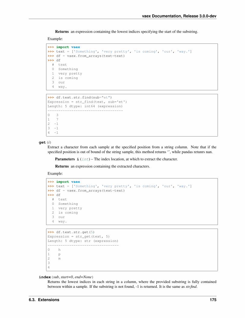
vaex Documentation, Release 3.0.0-dev
Returns an expression containing the lowest indices specifying the start of the substring.
Example:
>>> import vaex>>> text = ['Something', 'very pretty', 'is coming', 'our', 'way.']>>> df = vaex.from_arrays(text=text)>>> df
# text0 Something1 very pretty2 is coming3 our4 way.
>>> df.text.str.find(sub="et")Expression = str_find(text, sub='et')Length: 5 dtype: int64 (expression)-----------------------------------0 31 72 -13 -14 -1
get(i)Extract a character from each sample at the specified position from a string column. Note that if thespecified position is out of bound of the string sample, this method returns ‘’, while pandas retunrs nan.
Parameters i (int) – The index location, at which to extract the character.
Returns an expression containing the extracted characters.
Example:
>>> import vaex>>> text = ['Something', 'very pretty', 'is coming', 'our', 'way.']>>> df = vaex.from_arrays(text=text)>>> df
# text0 Something1 very pretty2 is coming3 our4 way.
>>> df.text.str.get(5)Expression = str_get(text, 5)Length: 5 dtype: str (expression)---------------------------------0 h1 p2 m34
index(sub, start=0, end=None)Returns the lowest indices in each string in a column, where the provided substring is fully containedbetween within a sample. If the substring is not found, -1 is returned. It is the same as str.find.
6.3. Extensions 175

vaex Documentation, Release 3.0.0-dev
Parameters
• sub (str) – A substring to be found in the samples
• start (int) –
• end (int) –
Returns an expression containing the lowest indices specifying the start of the substring.
Example:
>>> import vaex>>> text = ['Something', 'very pretty', 'is coming', 'our', 'way.']>>> df = vaex.from_arrays(text=text)>>> df
# text0 Something1 very pretty2 is coming3 our4 way.
>>> df.text.str.index(sub="et")Expression = str_find(text, sub='et')Length: 5 dtype: int64 (expression)-----------------------------------0 31 72 -13 -14 -1
isalnum()Check if all characters in a string sample are alphanumeric.
Returns an expression evaluated to True if a sample contains only alphanumeric characters,otherwise False.
Example:
>>> import vaex>>> text = ['Something', 'very pretty', 'is coming', 'our', 'way.']>>> df = vaex.from_arrays(text=text)>>> df
# text0 Something1 very pretty2 is coming3 our4 way.
>>> df.text.str.isalnum()Expression = str_isalnum(text)Length: 5 dtype: bool (expression)----------------------------------0 True1 False2 False
(continues on next page)
176 Chapter 6. API documentation for vaex library

vaex Documentation, Release 3.0.0-dev
(continued from previous page)
3 True4 False
isalpha()Check if all characters in a string sample are alphabetic.
Returns an expression evaluated to True if a sample contains only alphabetic characters, other-wise False.
Example:
>>> import vaex>>> text = ['Something', 'very pretty', 'is coming', 'our', 'way.']>>> df = vaex.from_arrays(text=text)>>> df
# text0 Something1 very pretty2 is coming3 our4 way.
>>> df.text.str.isalpha()Expression = str_isalpha(text)Length: 5 dtype: bool (expression)----------------------------------0 True1 False2 False3 True4 False
isdigit()Check if all characters in a string sample are digits.
Returns an expression evaluated to True if a sample contains only digits, otherwise False.
Example:
>>> import vaex>>> text = ['Something', 'very pretty', 'is coming', 'our', '6']>>> df = vaex.from_arrays(text=text)>>> df
# text0 Something1 very pretty2 is coming3 our4 6
>>> df.text.str.isdigit()Expression = str_isdigit(text)Length: 5 dtype: bool (expression)----------------------------------0 False1 False2 False
(continues on next page)
6.3. Extensions 177

vaex Documentation, Release 3.0.0-dev
(continued from previous page)
3 False4 True
islower()Check if all characters in a string sample are lowercase characters.
Returns an expression evaluated to True if a sample contains only lowercase characters, other-wise False.
Example:
>>> import vaex>>> text = ['Something', 'very pretty', 'is coming', 'our', 'way.']>>> df = vaex.from_arrays(text=text)>>> df
# text0 Something1 very pretty2 is coming3 our4 way.
>>> df.text.str.islower()Expression = str_islower(text)Length: 5 dtype: bool (expression)----------------------------------0 False1 True2 True3 True4 True
isspace()Check if all characters in a string sample are whitespaces.
Returns an expression evaluated to True if a sample contains only whitespaces, otherwise False.
Example:
>>> import vaex>>> text = ['Something', 'very pretty', 'is coming', ' ', ' ']>>> df = vaex.from_arrays(text=text)>>> df
# text0 Something1 very pretty2 is coming34
>>> df.text.str.isspace()Expression = str_isspace(text)Length: 5 dtype: bool (expression)----------------------------------0 False1 False2 False
(continues on next page)
178 Chapter 6. API documentation for vaex library

vaex Documentation, Release 3.0.0-dev
(continued from previous page)
3 True4 True
isupper()Check if all characters in a string sample are lowercase characters.
Returns an expression evaluated to True if a sample contains only lowercase characters, other-wise False.
Example:
>>> import vaex>>> text = ['SOMETHING', 'very pretty', 'is coming', 'our', 'way.']>>> df = vaex.from_arrays(text=text)>>> df
# text0 SOMETHING1 very pretty2 is coming3 our4 way.
>>> df.text.str.isupper()Expression = str_isupper(text)Length: 5 dtype: bool (expression)----------------------------------0 True1 False2 False3 False4 False
join(sep)Same as find (difference with pandas is that it does not raise a ValueError)
len()Returns the length of a string sample.
Returns an expression contains the length of each sample of a string column.
Example:
>>> import vaex>>> text = ['Something', 'very pretty', 'is coming', 'our', 'way.']>>> df = vaex.from_arrays(text=text)>>> df
# text0 Something1 very pretty2 is coming3 our4 way.
>>> df.text.str.len()Expression = str_len(text)Length: 5 dtype: int64 (expression)-----------------------------------
(continues on next page)
6.3. Extensions 179

vaex Documentation, Release 3.0.0-dev
(continued from previous page)
0 91 112 93 34 4
ljust(width, fillchar=’ ’)Fills the right side of string samples with a specified character such that the strings are right-hand justified.
Parameters
• width (int) – The minimal width of the strings.
• fillchar (str) – The character used for filling.
Returns an expression containing the filled strings.
Example:
>>> import vaex>>> text = ['Something', 'very pretty', 'is coming', 'our', 'way.']>>> df = vaex.from_arrays(text=text)>>> df
# text0 Something1 very pretty2 is coming3 our4 way.
>>> df.text.str.ljust(width=10, fillchar='!')Expression = str_ljust(text, width=10, fillchar='!')Length: 5 dtype: str (expression)---------------------------------0 Something!1 very pretty2 is coming!3 our!!!!!!!4 way.!!!!!!
lower()Converts string samples to lower case.
Returns an expression containing the converted strings.
Example:
>>> import vaex>>> text = ['Something', 'very pretty', 'is coming', 'our', 'way.']>>> df = vaex.from_arrays(text=text)>>> df
# text0 Something1 very pretty2 is coming3 our4 way.
180 Chapter 6. API documentation for vaex library

vaex Documentation, Release 3.0.0-dev
>>> df.text.str.lower()Expression = str_lower(text)Length: 5 dtype: str (expression)---------------------------------0 something1 very pretty2 is coming3 our4 way.
lstrip(to_strip=None)Remove leading characters from a string sample.
Parameters to_strip (str) – The string to be removed
Returns an expression containing the modified string column.
Example:
>>> import vaex>>> text = ['Something', 'very pretty', 'is coming', 'our', 'way.']>>> df = vaex.from_arrays(text=text)>>> df
# text0 Something1 very pretty2 is coming3 our4 way.
>>> df.text.str.lstrip(to_strip='very ')Expression = str_lstrip(text, to_strip='very ')Length: 5 dtype: str (expression)---------------------------------0 Something1 pretty2 is coming3 our4 way.
match(pattern)Check if a string sample matches a given regular expression.
Parameters pattern (str) – a string or regex to match to a string sample.
Returns an expression which is evaluated to True if a match is found, False otherwise.
Example:
>>> import vaex>>> text = ['Something', 'very pretty', 'is coming', 'our', 'way.']>>> df = vaex.from_arrays(text=text)>>> df
# text0 Something1 very pretty2 is coming3 our4 way.
6.3. Extensions 181

vaex Documentation, Release 3.0.0-dev
>>> df.text.str.match(pattern='our')Expression = str_match(text, pattern='our')Length: 5 dtype: bool (expression)----------------------------------0 False1 False2 False3 True4 False
pad(width, side=’left’, fillchar=’ ’)Pad strings in a given column.
Parameters
• width (int) – The total width of the string
• side (str) – If ‘left’ than pad on the left, if ‘right’ than pad on the right side the string.
• fillchar (str) – The character used for padding.
Returns an expression containing the padded strings.
Example:
>>> import vaex>>> text = ['Something', 'very pretty', 'is coming', 'our', 'way.']>>> df = vaex.from_arrays(text=text)>>> df
# text0 Something1 very pretty2 is coming3 our4 way.
>>> df.text.str.pad(width=10, side='left', fillchar='!')Expression = str_pad(text, width=10, side='left', fillchar='!')Length: 5 dtype: str (expression)---------------------------------0 !Something1 very pretty2 !is coming3 !!!!!!!our4 !!!!!!way.
repeat(repeats)Duplicate each string in a column.
Parameters repeats (int) – number of times each string sample is to be duplicated.
Returns an expression containing the duplicated strings
Example:
>>> import vaex>>> text = ['Something', 'very pretty', 'is coming', 'our', 'way.']>>> df = vaex.from_arrays(text=text)>>> df
# text
(continues on next page)
182 Chapter 6. API documentation for vaex library

vaex Documentation, Release 3.0.0-dev
(continued from previous page)
0 Something1 very pretty2 is coming3 our4 way.
>>> df.text.str.repeat(3)Expression = str_repeat(text, 3)Length: 5 dtype: str (expression)---------------------------------0 SomethingSomethingSomething1 very prettyvery prettyvery pretty2 is comingis comingis coming3 ourourour4 way.way.way.
replace(pat, repl, n=-1, flags=0, regex=False)Replace occurences of a pattern/regex in a column with some other string.
Parameters
• pattern (str) – string or a regex pattern
• replace (str) – a replacement string
• n (int) – number of replacements to be made from the start. If -1 make all replacements.
• flags (int) – ??
• regex (bool) – If True, . . . ?
Returns an expression containing the string replacements.
Example:
>>> import vaex>>> text = ['Something', 'very pretty', 'is coming', 'our', 'way.']>>> df = vaex.from_arrays(text=text)>>> df
# text0 Something1 very pretty2 is coming3 our4 way.
>>> df.text.str.replace(pat='et', repl='__')Expression = str_replace(text, pat='et', repl='__')Length: 5 dtype: str (expression)---------------------------------0 Som__hing1 very pr__ty2 is coming3 our4 way.
rfind(sub, start=0, end=None)Returns the highest indices in each string in a column, where the provided substring is fully containedbetween within a sample. If the substring is not found, -1 is returned.
6.3. Extensions 183

vaex Documentation, Release 3.0.0-dev
Parameters
• sub (str) – A substring to be found in the samples
• start (int) –
• end (int) –
Returns an expression containing the highest indices specifying the start of the substring.
Example:
>>> import vaex>>> text = ['Something', 'very pretty', 'is coming', 'our', 'way.']>>> df = vaex.from_arrays(text=text)>>> df
# text0 Something1 very pretty2 is coming3 our4 way.
>>> df.text.str.rfind(sub="et")Expression = str_rfind(text, sub='et')Length: 5 dtype: int64 (expression)-----------------------------------0 31 72 -13 -14 -1
rindex(sub, start=0, end=None)Returns the highest indices in each string in a column, where the provided substring is fully containedbetween within a sample. If the substring is not found, -1 is returned. Same as str.rfind.
Parameters
• sub (str) – A substring to be found in the samples
• start (int) –
• end (int) –
Returns an expression containing the highest indices specifying the start of the substring.
Example:
>>> import vaex>>> text = ['Something', 'very pretty', 'is coming', 'our', 'way.']>>> df = vaex.from_arrays(text=text)>>> df
# text0 Something1 very pretty2 is coming3 our4 way.
184 Chapter 6. API documentation for vaex library

vaex Documentation, Release 3.0.0-dev
>>> df.text.str.rindex(sub="et")Expression = str_rindex(text, sub='et')Length: 5 dtype: int64 (expression)-----------------------------------0 31 72 -13 -14 -1
rjust(width, fillchar=’ ’)Fills the left side of string samples with a specified character such that the strings are left-hand justified.
Parameters
• width (int) – The minimal width of the strings.
• fillchar (str) – The character used for filling.
Returns an expression containing the filled strings.
Example:
>>> import vaex>>> text = ['Something', 'very pretty', 'is coming', 'our', 'way.']>>> df = vaex.from_arrays(text=text)>>> df
# text0 Something1 very pretty2 is coming3 our4 way.
>>> df.text.str.rjust(width=10, fillchar='!')Expression = str_rjust(text, width=10, fillchar='!')Length: 5 dtype: str (expression)---------------------------------0 !Something1 very pretty2 !is coming3 !!!!!!!our4 !!!!!!way.
rstrip(to_strip=None)Remove trailing characters from a string sample.
Parameters to_strip (str) – The string to be removed
Returns an expression containing the modified string column.
Example:
>>> import vaex>>> text = ['Something', 'very pretty', 'is coming', 'our', 'way.']>>> df = vaex.from_arrays(text=text)>>> df
# text0 Something1 very pretty
(continues on next page)
6.3. Extensions 185

vaex Documentation, Release 3.0.0-dev
(continued from previous page)
2 is coming3 our4 way.
>>> df.text.str.rstrip(to_strip='ing')Expression = str_rstrip(text, to_strip='ing')Length: 5 dtype: str (expression)---------------------------------0 Someth1 very pretty2 is com3 our4 way.
slice(start=0, stop=None)Slice substrings from each string element in a column.
Parameters
• start (int) – The start position for the slice operation.
• end (int) – The stop position for the slice operation.
Returns an expression containing the sliced substrings.
Example:
>>> import vaex>>> text = ['Something', 'very pretty', 'is coming', 'our', 'way.']>>> df = vaex.from_arrays(text=text)>>> df
# text0 Something1 very pretty2 is coming3 our4 way.
>>> df.text.str.slice(start=2, stop=5)Expression = str_pandas_slice(text, start=2, stop=5)Length: 5 dtype: str (expression)---------------------------------0 met1 ry2 co3 r4 y.
startswith(pat)Check if a start of a string matches a pattern.
Parameters pat (str) – A string pattern. Regular expressions are not supported.
Returns an expression which is evaluated to True if the pattern is found at the start of a stringsample, False otherwise.
Example:
186 Chapter 6. API documentation for vaex library

vaex Documentation, Release 3.0.0-dev
>>> import vaex>>> text = ['Something', 'very pretty', 'is coming', 'our', 'way.']>>> df = vaex.from_arrays(text=text)>>> df
# text0 Something1 very pretty2 is coming3 our4 way.
>>> df.text.str.startswith(pat='is')Expression = str_startswith(text, pat='is')Length: 5 dtype: bool (expression)----------------------------------0 False1 False2 True3 False4 False
strip(to_strip=None)Removes leading and trailing characters.
Strips whitespaces (including new lines), or a set of specified characters from each string saple in a column,both from the left right sides.
Parameters
• to_strip (str) – The characters to be removed. All combinations of the characterswill be removed. If None, it removes whitespaces.
• returns – an expression containing the modified string samples.
Example:
>>> import vaex>>> text = ['Something', 'very pretty', 'is coming', 'our', 'way.']>>> df = vaex.from_arrays(text=text)>>> df
# text0 Something1 very pretty2 is coming3 our4 way.
>>> df.text.str.strip(to_strip='very')Expression = str_strip(text, to_strip='very')Length: 5 dtype: str (expression)---------------------------------0 Something1 prett2 is coming3 ou4 way.
title()Converts all string samples to titlecase.
6.3. Extensions 187

vaex Documentation, Release 3.0.0-dev
Returns an expression containing the converted strings.
Example:
>>> import vaex>>> text = ['Something', 'very pretty', 'is coming', 'our', 'way.']>>> df = vaex.from_arrays(text=text)>>> df
# text0 Something1 very pretty2 is coming3 our4 way.
>>> df.text.str.title()Expression = str_title(text)Length: 5 dtype: str (expression)---------------------------------0 Something1 Very Pretty2 Is Coming3 Our4 Way.
upper()Converts all strings in a column to uppercase.
Returns an expression containing the converted strings.
Example:
>>> import vaex>>> text = ['Something', 'very pretty', 'is coming', 'our', 'way.']>>> df = vaex.from_arrays(text=text)>>> df
# text0 Something1 very pretty2 is coming3 our4 way.
>>> df.text.str.upper()Expression = str_upper(text)Length: 5 dtype: str (expression)---------------------------------0 SOMETHING1 VERY PRETTY2 IS COMING3 OUR4 WAY.
zfill(width)Pad strings in a column by prepanding “0” characters.
Parameters width (int) – The minimum length of the resulting string. Strings shorter lessthan width will be prepended with zeros.
Returns an expression containing the modified strings.
188 Chapter 6. API documentation for vaex library

vaex Documentation, Release 3.0.0-dev
Example:
>>> import vaex>>> text = ['Something', 'very pretty', 'is coming', 'our', 'way.']>>> df = vaex.from_arrays(text=text)>>> df
# text0 Something1 very pretty2 is coming3 our4 way.
>>> df.text.str.zfill(width=12)Expression = str_zfill(text, width=12)Length: 5 dtype: str (expression)---------------------------------0 000Something1 0very pretty2 000is coming3 000000000our4 00000000way.
6.3.2 String (pandas) operations
class vaex.expression.StringOperationsPandas(expression)Bases: object
String operations using Pandas Series (much slower)
__init__(expression)Initialize self. See help(type(self)) for accurate signature.
__weakref__list of weak references to the object (if defined)
byte_length(**kwargs)Wrapper around pandas.Series.byte_length
capitalize(**kwargs)Wrapper around pandas.Series.capitalize
cat(**kwargs)Wrapper around pandas.Series.cat
center(**kwargs)Wrapper around pandas.Series.center
contains(**kwargs)Wrapper around pandas.Series.contains
count(**kwargs)Wrapper around pandas.Series.count
endswith(**kwargs)Wrapper around pandas.Series.endswith
equals(**kwargs)Wrapper around pandas.Series.equals
6.3. Extensions 189

vaex Documentation, Release 3.0.0-dev
find(**kwargs)Wrapper around pandas.Series.find
get(**kwargs)Wrapper around pandas.Series.get
index(**kwargs)Wrapper around pandas.Series.index
isalnum(**kwargs)Wrapper around pandas.Series.isalnum
isalpha(**kwargs)Wrapper around pandas.Series.isalpha
isdigit(**kwargs)Wrapper around pandas.Series.isdigit
islower(**kwargs)Wrapper around pandas.Series.islower
isspace(**kwargs)Wrapper around pandas.Series.isspace
isupper(**kwargs)Wrapper around pandas.Series.isupper
join(**kwargs)Wrapper around pandas.Series.join
len(**kwargs)Wrapper around pandas.Series.len
ljust(**kwargs)Wrapper around pandas.Series.ljust
lower(**kwargs)Wrapper around pandas.Series.lower
lstrip(**kwargs)Wrapper around pandas.Series.lstrip
match(**kwargs)Wrapper around pandas.Series.match
pad(**kwargs)Wrapper around pandas.Series.pad
repeat(**kwargs)Wrapper around pandas.Series.repeat
replace(**kwargs)Wrapper around pandas.Series.replace
rfind(**kwargs)Wrapper around pandas.Series.rfind
rindex(**kwargs)Wrapper around pandas.Series.rindex
rjust(**kwargs)Wrapper around pandas.Series.rjust
190 Chapter 6. API documentation for vaex library

vaex Documentation, Release 3.0.0-dev
rstrip(**kwargs)Wrapper around pandas.Series.rstrip
slice(**kwargs)Wrapper around pandas.Series.slice
split(**kwargs)Wrapper around pandas.Series.split
startswith(**kwargs)Wrapper around pandas.Series.startswith
strip(**kwargs)Wrapper around pandas.Series.strip
title(**kwargs)Wrapper around pandas.Series.title
upper(**kwargs)Wrapper around pandas.Series.upper
zfill(**kwargs)Wrapper around pandas.Series.zfill
6.3.3 Date/time operations
class vaex.expression.DateTime(expression)Bases: object
DateTime operations
Usually accessed using e.g. df.birthday.dt.dayofweek
__init__(expression)Initialize self. See help(type(self)) for accurate signature.
__weakref__list of weak references to the object (if defined)
dayExtracts the day from a datetime sample.
Returns an expression containing the day extracted from a datetime column.
Example:
>>> import vaex>>> import numpy as np>>> date = np.array(['2009-10-12T03:31:00', '2016-02-11T10:17:34', '2015-11-→˓12T11:34:22'], dtype=np.datetime64)>>> df = vaex.from_arrays(date=date)>>> df
# date0 2009-10-12 03:31:001 2016-02-11 10:17:342 2015-11-12 11:34:22
>>> df.date.dt.dayExpression = dt_day(date)Length: 3 dtype: int64 (expression)
(continues on next page)
6.3. Extensions 191

vaex Documentation, Release 3.0.0-dev
(continued from previous page)
-----------------------------------0 121 112 12
day_nameReturns the day names of a datetime sample in English.
Returns an expression containing the day names extracted from a datetime column.
Example:
>>> import vaex>>> import numpy as np>>> date = np.array(['2009-10-12T03:31:00', '2016-02-11T10:17:34', '2015-11-→˓12T11:34:22'], dtype=np.datetime64)>>> df = vaex.from_arrays(date=date)>>> df
# date0 2009-10-12 03:31:001 2016-02-11 10:17:342 2015-11-12 11:34:22
>>> df.date.dt.day_nameExpression = dt_day_name(date)Length: 3 dtype: str (expression)---------------------------------0 Monday1 Thursday2 Thursday
dayofweekObtain the day of the week with Monday=0 and Sunday=6
Returns an expression containing the day of week.
Example:
>>> import vaex>>> import numpy as np>>> date = np.array(['2009-10-12T03:31:00', '2016-02-11T10:17:34', '2015-11-→˓12T11:34:22'], dtype=np.datetime64)>>> df = vaex.from_arrays(date=date)>>> df
# date0 2009-10-12 03:31:001 2016-02-11 10:17:342 2015-11-12 11:34:22
>>> df.date.dt.dayofweekExpression = dt_dayofweek(date)Length: 3 dtype: int64 (expression)-----------------------------------0 01 32 3
192 Chapter 6. API documentation for vaex library
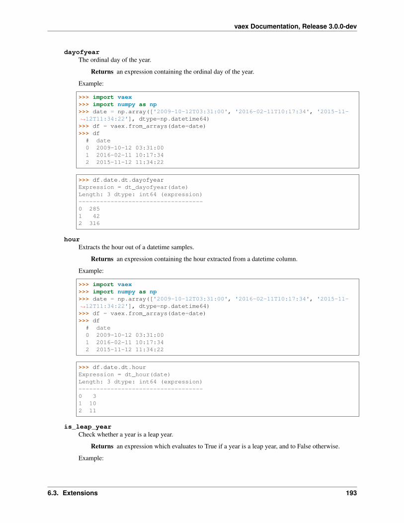
vaex Documentation, Release 3.0.0-dev
dayofyearThe ordinal day of the year.
Returns an expression containing the ordinal day of the year.
Example:
>>> import vaex>>> import numpy as np>>> date = np.array(['2009-10-12T03:31:00', '2016-02-11T10:17:34', '2015-11-→˓12T11:34:22'], dtype=np.datetime64)>>> df = vaex.from_arrays(date=date)>>> df
# date0 2009-10-12 03:31:001 2016-02-11 10:17:342 2015-11-12 11:34:22
>>> df.date.dt.dayofyearExpression = dt_dayofyear(date)Length: 3 dtype: int64 (expression)-----------------------------------0 2851 422 316
hourExtracts the hour out of a datetime samples.
Returns an expression containing the hour extracted from a datetime column.
Example:
>>> import vaex>>> import numpy as np>>> date = np.array(['2009-10-12T03:31:00', '2016-02-11T10:17:34', '2015-11-→˓12T11:34:22'], dtype=np.datetime64)>>> df = vaex.from_arrays(date=date)>>> df
# date0 2009-10-12 03:31:001 2016-02-11 10:17:342 2015-11-12 11:34:22
>>> df.date.dt.hourExpression = dt_hour(date)Length: 3 dtype: int64 (expression)-----------------------------------0 31 102 11
is_leap_yearCheck whether a year is a leap year.
Returns an expression which evaluates to True if a year is a leap year, and to False otherwise.
Example:
6.3. Extensions 193
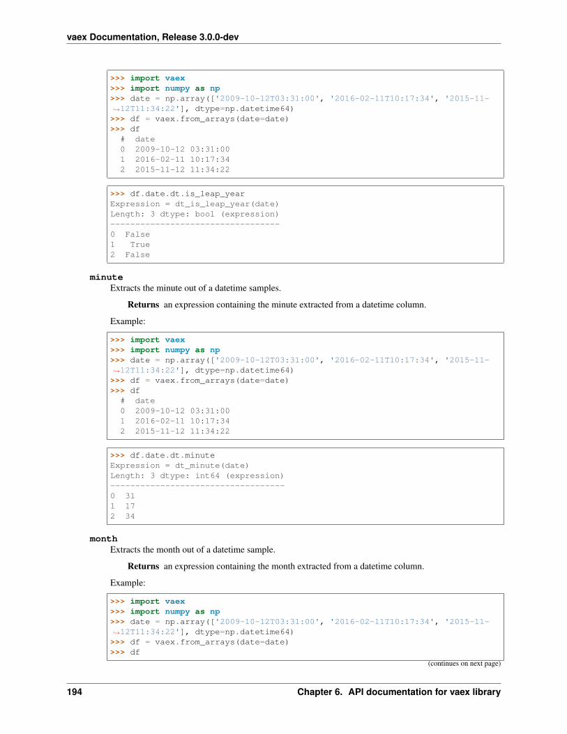
vaex Documentation, Release 3.0.0-dev
>>> import vaex>>> import numpy as np>>> date = np.array(['2009-10-12T03:31:00', '2016-02-11T10:17:34', '2015-11-→˓12T11:34:22'], dtype=np.datetime64)>>> df = vaex.from_arrays(date=date)>>> df
# date0 2009-10-12 03:31:001 2016-02-11 10:17:342 2015-11-12 11:34:22
>>> df.date.dt.is_leap_yearExpression = dt_is_leap_year(date)Length: 3 dtype: bool (expression)----------------------------------0 False1 True2 False
minuteExtracts the minute out of a datetime samples.
Returns an expression containing the minute extracted from a datetime column.
Example:
>>> import vaex>>> import numpy as np>>> date = np.array(['2009-10-12T03:31:00', '2016-02-11T10:17:34', '2015-11-→˓12T11:34:22'], dtype=np.datetime64)>>> df = vaex.from_arrays(date=date)>>> df
# date0 2009-10-12 03:31:001 2016-02-11 10:17:342 2015-11-12 11:34:22
>>> df.date.dt.minuteExpression = dt_minute(date)Length: 3 dtype: int64 (expression)-----------------------------------0 311 172 34
monthExtracts the month out of a datetime sample.
Returns an expression containing the month extracted from a datetime column.
Example:
>>> import vaex>>> import numpy as np>>> date = np.array(['2009-10-12T03:31:00', '2016-02-11T10:17:34', '2015-11-→˓12T11:34:22'], dtype=np.datetime64)>>> df = vaex.from_arrays(date=date)>>> df
(continues on next page)
194 Chapter 6. API documentation for vaex library

vaex Documentation, Release 3.0.0-dev
(continued from previous page)
# date0 2009-10-12 03:31:001 2016-02-11 10:17:342 2015-11-12 11:34:22
>>> df.date.dt.monthExpression = dt_month(date)Length: 3 dtype: int64 (expression)-----------------------------------0 101 22 11
month_nameReturns the month names of a datetime sample in English.
Returns an expression containing the month names extracted from a datetime column.
Example:
>>> import vaex>>> import numpy as np>>> date = np.array(['2009-10-12T03:31:00', '2016-02-11T10:17:34', '2015-11-→˓12T11:34:22'], dtype=np.datetime64)>>> df = vaex.from_arrays(date=date)>>> df
# date0 2009-10-12 03:31:001 2016-02-11 10:17:342 2015-11-12 11:34:22
>>> df.date.dt.month_nameExpression = dt_month_name(date)Length: 3 dtype: str (expression)---------------------------------0 October1 February2 November
quarterExtracts the quarter from a datetime sample.
Returns an expression containing the number of the quarter extracted from a datetime column.
Example:
>>> import vaex>>> import numpy as np>>> date = np.array(['2009-10-12T03:31:00', '2016-02-11T10:17:34', '2015-11-→˓12T11:34:22'], dtype=np.datetime64)>>> df = vaex.from_arrays(date=date)>>> df
# date0 2009-10-12 03:31:001 2016-02-11 10:17:342 2015-11-12 11:34:22
6.3. Extensions 195

vaex Documentation, Release 3.0.0-dev
>>> df.date.dt.quarterExpression = dt_quarter(date)Length: 3 dtype: int64 (expression)-----------------------------------0 41 12 4
secondExtracts the second out of a datetime samples.
Returns an expression containing the second extracted from a datetime column.
Example:
>>> import vaex>>> import numpy as np>>> date = np.array(['2009-10-12T03:31:00', '2016-02-11T10:17:34', '2015-11-→˓12T11:34:22'], dtype=np.datetime64)>>> df = vaex.from_arrays(date=date)>>> df
# date0 2009-10-12 03:31:001 2016-02-11 10:17:342 2015-11-12 11:34:22
>>> df.date.dt.secondExpression = dt_second(date)Length: 3 dtype: int64 (expression)-----------------------------------0 01 342 22
strftime(date_format)Returns a formatted string from a datetime sample.
Returns an expression containing a formatted string extracted from a datetime column.
Example:
>>> import vaex>>> import numpy as np>>> date = np.array(['2009-10-12T03:31:00', '2016-02-11T10:17:34', '2015-11-→˓12T11:34:22'], dtype=np.datetime64)>>> df = vaex.from_arrays(date=date)>>> df
# date0 2009-10-12 03:31:001 2016-02-11 10:17:342 2015-11-12 11:34:22
>>> df.date.dt.strftime("%Y-%m")Expression = dt_strftime(date, '%Y-%m')Length: 3 dtype: object (expression)------------------------------------0 2009-10
(continues on next page)
196 Chapter 6. API documentation for vaex library

vaex Documentation, Release 3.0.0-dev
(continued from previous page)
1 2016-022 2015-11
weekofyearReturns the week ordinal of the year.
Returns an expression containing the week ordinal of the year, extracted from a datetime col-umn.
Example:
>>> import vaex>>> import numpy as np>>> date = np.array(['2009-10-12T03:31:00', '2016-02-11T10:17:34', '2015-11-→˓12T11:34:22'], dtype=np.datetime64)>>> df = vaex.from_arrays(date=date)>>> df
# date0 2009-10-12 03:31:001 2016-02-11 10:17:342 2015-11-12 11:34:22
>>> df.date.dt.weekofyearExpression = dt_weekofyear(date)Length: 3 dtype: int64 (expression)-----------------------------------0 421 62 46
yearExtracts the year out of a datetime sample.
Returns an expression containing the year extracted from a datetime column.
Example:
>>> import vaex>>> import numpy as np>>> date = np.array(['2009-10-12T03:31:00', '2016-02-11T10:17:34', '2015-11-→˓12T11:34:22'], dtype=np.datetime64)>>> df = vaex.from_arrays(date=date)>>> df
# date0 2009-10-12 03:31:001 2016-02-11 10:17:342 2015-11-12 11:34:22
>>> df.date.dt.yearExpression = dt_year(date)Length: 3 dtype: int64 (expression)-----------------------------------0 20091 20162 2015
6.3. Extensions 197

vaex Documentation, Release 3.0.0-dev
6.3.4 Timedelta operations
class vaex.expression.TimeDelta(expression)Bases: object
TimeDelta operations
Usually accessed using e.g. df.delay.td.days
__init__(expression)Initialize self. See help(type(self)) for accurate signature.
__weakref__list of weak references to the object (if defined)
daysNumber of days in each timedelta sample.
Returns an expression containing the number of days in a timedelta sample.
Example:
>>> import vaex>>> import numpy as np>>> delta = np.array([17658720110, 11047049384039, 40712636304958, -→˓18161254954], dtype='timedelta64[s]')>>> df = vaex.from_arrays(delta=delta)>>> df
# delta0 204 days +9:12:001 1 days +6:41:102 471 days +5:03:563 -22 days +23:31:15
>>> df.delta.td.daysExpression = td_days(delta)Length: 4 dtype: int64 (expression)-----------------------------------0 2041 12 4713 -22
microsecondsNumber of microseconds (>= 0 and less than 1 second) in each timedelta sample.
Returns an expression containing the number of microseconds in a timedelta sample.
Example:
>>> import vaex>>> import numpy as np>>> delta = np.array([17658720110, 11047049384039, 40712636304958, -→˓18161254954], dtype='timedelta64[s]')>>> df = vaex.from_arrays(delta=delta)>>> df
# delta0 204 days +9:12:001 1 days +6:41:102 471 days +5:03:563 -22 days +23:31:15
198 Chapter 6. API documentation for vaex library

vaex Documentation, Release 3.0.0-dev
>>> df.delta.td.microsecondsExpression = td_microseconds(delta)Length: 4 dtype: int64 (expression)-----------------------------------0 2904481 9785822 195833 709551
nanosecondsNumber of nanoseconds (>= 0 and less than 1 microsecond) in each timedelta sample.
Returns an expression containing the number of nanoseconds in a timedelta sample.
Example:
>>> import vaex>>> import numpy as np>>> delta = np.array([17658720110, 11047049384039, 40712636304958, -→˓18161254954], dtype='timedelta64[s]')>>> df = vaex.from_arrays(delta=delta)>>> df
# delta0 204 days +9:12:001 1 days +6:41:102 471 days +5:03:563 -22 days +23:31:15
>>> df.delta.td.nanosecondsExpression = td_nanoseconds(delta)Length: 4 dtype: int64 (expression)-----------------------------------0 3841 162 4883 616
secondsNumber of seconds (>= 0 and less than 1 day) in each timedelta sample.
Returns an expression containing the number of seconds in a timedelta sample.
Example:
>>> import vaex>>> import numpy as np>>> delta = np.array([17658720110, 11047049384039, 40712636304958, -→˓18161254954], dtype='timedelta64[s]')>>> df = vaex.from_arrays(delta=delta)>>> df
# delta0 204 days +9:12:001 1 days +6:41:102 471 days +5:03:563 -22 days +23:31:15
>>> df.delta.td.secondsExpression = td_seconds(delta)
(continues on next page)
6.3. Extensions 199

vaex Documentation, Release 3.0.0-dev
(continued from previous page)
Length: 4 dtype: int64 (expression)-----------------------------------0 304361 390862 286813 23519
total_seconds()Total duration of each timedelta sample expressed in seconds.
Returns an expression containing the total number of seconds in a timedelta sample.
Example: >>> import vaex >>> import numpy as np >>> delta = np.array([17658720110,11047049384039, 40712636304958, -18161254954], dtype=’timedelta64[s]’) >>> df =vaex.from_arrays(delta=delta) >>> df
# delta 0 204 days +9:12:00 1 1 days +6:41:10 2 471 days +5:03:56 3 -22 days +23:31:15
>>> df.delta.td.total_seconds()Expression = td_total_seconds(delta)Length: 4 dtype: float64 (expression)-------------------------------------0 -7.88024e+081 -2.55032e+092 6.72134e+083 2.85489e+08
6.3.5 Geo operations
class vaex.geo.DataFrameAccessorGeo(df)Bases: object
Geometry/geographic helper methods
Example:
>>> df_xyz = df.geo.spherical2cartesian(df.longitude, df.latitude, df.distance)>>> df_xyz.x.mean()
__init__(df)Initialize self. See help(type(self)) for accurate signature.
__weakref__list of weak references to the object (if defined)
bearing(lon1, lat1, lon2, lat2, bearing=’bearing’, inplace=False)Calculates a bearing, based on http://www.movable-type.co.uk/scripts/latlong.html
cartesian2spherical(x=’x’, y=’y’, z=’z’, alpha=’l’, delta=’b’, distance=’distance’, radi-ans=False, center=None, center_name=’solar_position’, inplace=False)
Convert cartesian to spherical coordinates.
Parameters
• x –
• y –
• z –
200 Chapter 6. API documentation for vaex library
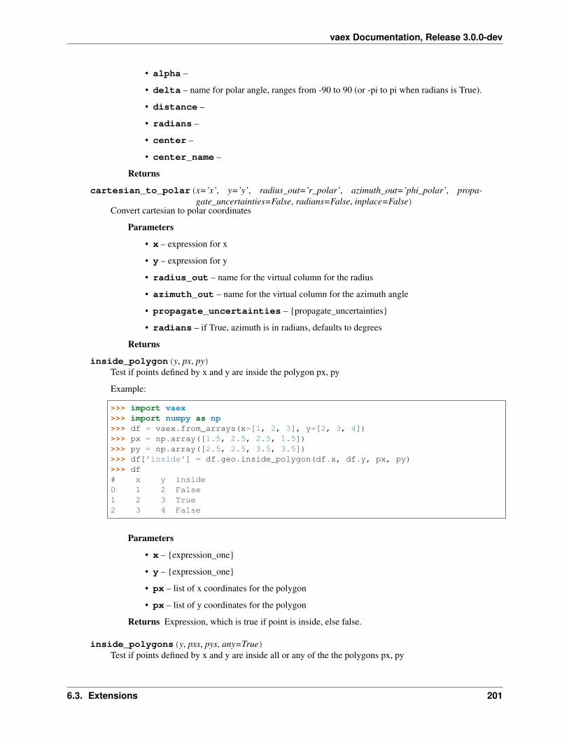
vaex Documentation, Release 3.0.0-dev
• alpha –
• delta – name for polar angle, ranges from -90 to 90 (or -pi to pi when radians is True).
• distance –
• radians –
• center –
• center_name –
Returns
cartesian_to_polar(x=’x’, y=’y’, radius_out=’r_polar’, azimuth_out=’phi_polar’, propa-gate_uncertainties=False, radians=False, inplace=False)
Convert cartesian to polar coordinates
Parameters
• x – expression for x
• y – expression for y
• radius_out – name for the virtual column for the radius
• azimuth_out – name for the virtual column for the azimuth angle
• propagate_uncertainties – {propagate_uncertainties}
• radians – if True, azimuth is in radians, defaults to degrees
Returns
inside_polygon(y, px, py)Test if points defined by x and y are inside the polygon px, py
Example:
>>> import vaex>>> import numpy as np>>> df = vaex.from_arrays(x=[1, 2, 3], y=[2, 3, 4])>>> px = np.array([1.5, 2.5, 2.5, 1.5])>>> py = np.array([2.5, 2.5, 3.5, 3.5])>>> df['inside'] = df.geo.inside_polygon(df.x, df.y, px, py)>>> df# x y inside0 1 2 False1 2 3 True2 3 4 False
Parameters
• x – {expression_one}
• y – {expression_one}
• px – list of x coordinates for the polygon
• px – list of y coordinates for the polygon
Returns Expression, which is true if point is inside, else false.
inside_polygons(y, pxs, pys, any=True)Test if points defined by x and y are inside all or any of the the polygons px, py
6.3. Extensions 201

vaex Documentation, Release 3.0.0-dev
Example:
>>> import vaex>>> import numpy as np>>> df = vaex.from_arrays(x=[1, 2, 3], y=[2, 3, 4])>>> px = np.array([1.5, 2.5, 2.5, 1.5])>>> py = np.array([2.5, 2.5, 3.5, 3.5])>>> df['inside'] = df.geo.inside_polygons(df.x, df.y, [px, px + 1], [py, py +→˓1], any=True)>>> df# x y inside0 1 2 False1 2 3 True2 3 4 True
Parameters
• x – {expression_one}
• y – {expression_one}
• pxs – list of N ndarrays with x coordinates for the polygon, N is the number of polygons
• pxs – list of N ndarrays with y coordinates for the polygon
• any – return true if in any polygon, or all polygons
Returns Expression , which is true if point is inside, else false.
inside_which_polygon(y, pxs, pys)Find in which polygon (0 based index) a point resides
Example:
>>> import vaex>>> import numpy as np>>> df = vaex.from_arrays(x=[1, 2, 3], y=[2, 3, 4])>>> px = np.array([1.5, 2.5, 2.5, 1.5])>>> py = np.array([2.5, 2.5, 3.5, 3.5])>>> df['polygon_index'] = df.geo.inside_which_polygon(df.x, df.y, [px, px +→˓1], [py, py + 1])>>> df# x y polygon_index0 1 2 --1 2 3 02 3 4 1
Parameters
• x – {expression_one}
• y – {expression_one}
• px – list of N ndarrays with x coordinates for the polygon, N is the number of polygons
• px – list of N ndarrays with y coordinates for the polygon
Returns Expression, 0 based index to which polygon the point belongs (or missing/maskedvalue)
202 Chapter 6. API documentation for vaex library

vaex Documentation, Release 3.0.0-dev
inside_which_polygons(x, y, pxss, pyss=None, any=True)Find in which set of polygons (0 based index) a point resides.
If any=True, it will be the first matching polygon set index, if any=False, it will be the first index thatmatches all polygons in the set.
>>> import vaex>>> import numpy as np>>> df = vaex.from_arrays(x=[1, 2, 3], y=[2, 3, 4])>>> px = np.array([1.5, 2.5, 2.5, 1.5])>>> py = np.array([2.5, 2.5, 3.5, 3.5])>>> polygonA = [px, py]>>> polygonB = [px + 1, py + 1]>>> pxs = [[polygonA, polygonB], [polygonA]]>>> df['polygon_index'] = df.geo.inside_which_polygons(df.x, df.y, pxs,→˓any=True)>>> df# x y polygon_index0 1 2 --1 2 3 02 3 4 0>>> df['polygon_index'] = df.geo.inside_which_polygons(df.x, df.y, pxs,→˓any=False)>>> df# x y polygon_index0 1 2 --1 2 3 12 3 4 --
Parameters
• x – expression in the form of a string, e.g. ‘x’ or ‘x+y’ or vaex expression object, e.g. df.xor df.x+df.y
• y – expression in the form of a string, e.g. ‘x’ or ‘x+y’ or vaex expression object, e.g. df.xor df.x+df.y
• px – list of N ndarrays with x coordinates for the polygon, N is the number of polygons
• px – list of N ndarrays with y coordinates for the polygon, if None, the shape of thendarrays of the last dimention of the x arrays should be 2 (i.e. have the x and y coordinates)
• any – test if point it in any polygon (logically or), or all polygons (logically and)
Returns Expression, 0 based index to which polygon the point belongs (or missing/maskedvalue)
project_aitoff(alpha, delta, x, y, radians=True, inplace=False)Add aitoff (https://en.wikipedia.org/wiki/Aitoff_projection) projection
Parameters
• alpha – azimuth angle
• delta – polar angle
• x – output name for x coordinate
• y – output name for y coordinate
• radians – input and output in radians (True), or degrees (False)
6.3. Extensions 203
vaex Documentation, Release 3.0.0-dev
Returns
project_gnomic(alpha, delta, alpha0=0, delta0=0, x=’x’, y=’y’, radians=False, postfix=”, in-place=False)
Adds a gnomic projection to the DataFrame
rotation_2d(x, y, xnew, ynew, angle_degrees, propagate_uncertainties=False, inplace=False)Rotation in 2d.
Parameters
• x (str) – Name/expression of x column
• y (str) – idem for y
• xnew (str) – name of transformed x column
• ynew (str) –
• angle_degrees (float) – rotation in degrees, anti clockwise
Returns
spherical2cartesian(alpha, delta, distance, xname=’x’, yname=’y’, zname=’z’, propa-gate_uncertainties=False, center=[0, 0, 0], radians=False, inplace=False)
Convert spherical to cartesian coordinates.
Parameters
• alpha –
• delta – polar angle, ranging from the -90 (south pole) to 90 (north pole)
• distance – radial distance, determines the units of x, y and z
• xname –
• yname –
• zname –
• propagate_uncertainties – If true, will propagate errors for the new virtualcolumns, see propagate_uncertainties() for details
• center –
• radians –
Returns New dataframe (in inplace is False) with new x,y,z columns
velocity_cartesian2polar(x=’x’, y=’y’, vx=’vx’, radius_polar=None, vy=’vy’,vr_out=’vr_polar’, vazimuth_out=’vphi_polar’, propa-gate_uncertainties=False, inplace=False)
Convert cartesian to polar velocities.
Parameters
• x –
• y –
• vx –
• radius_polar – Optional expression for the radius, may lead to a better performancewhen given.
• vy –
• vr_out –
204 Chapter 6. API documentation for vaex library

vaex Documentation, Release 3.0.0-dev
• vazimuth_out –
• propagate_uncertainties – If true, will propagate errors for the new virtualcolumns, see propagate_uncertainties() for details
Returns
velocity_cartesian2spherical(x=’x’, y=’y’, z=’z’, vx=’vx’, vy=’vy’, vz=’vz’, vr=’vr’,vlong=’vlong’, vlat=’vlat’, distance=None, inplace=False)
Convert velocities from a cartesian to a spherical coordinate system
TODO: uncertainty propagation
Parameters
• x – name of x column (input)
• y – y
• z – z
• vx – vx
• vy – vy
• vz – vz
• vr – name of the column for the radial velocity in the r direction (output)
• vlong – name of the column for the velocity component in the longitude direction (out-put)
• vlat – name of the column for the velocity component in the latitude direction, positivepoints to the north pole (output)
• distance – Expression for distance, if not given defaults to sqrt(x**2+y**2+z**2), butif this column already exists, passing this expression may lead to a better performance
Returns
velocity_polar2cartesian(x=’x’, y=’y’, azimuth=None, vr=’vr_polar’, vaz-imuth=’vphi_polar’, vx_out=’vx’, vy_out=’vy’, propa-gate_uncertainties=False, inplace=False)
Convert cylindrical polar velocities to Cartesian.
Parameters
• x –
• y –
• azimuth – Optional expression for the azimuth in degrees , may lead to a better perfor-mance when given.
• vr –
• vazimuth –
• vx_out –
• vy_out –
• propagate_uncertainties – If true, will propagate errors for the new virtualcolumns, see propagate_uncertainties() for details
6.3. Extensions 205

vaex Documentation, Release 3.0.0-dev
6.3.6 GraphQL operations
class vaex.graphql.DataFrameAccessorGraphQL(df)Bases: object
Exposes a GraphQL layer to a DataFrame
See the GraphQL example for more usage.
The easiest way to learn to use the GraphQL language/vaex interface is to launch a server, and play with theGraphiQL graphical interface, its autocomplete, and the schema explorer.
We try to stay close to the Hasura API: https://docs.hasura.io/1.0/graphql/manual/api-reference/graphql-api/query.html
__init__(df)Initialize self. See help(type(self)) for accurate signature.
__weakref__list of weak references to the object (if defined)
execute(*args, **kwargs)Creates a schema, and execute the query (first argument)
query(name=’df’)Creates a graphene query object exposing this DataFrame named name
schema(name=’df’, auto_camelcase=False, **kwargs)Creates a graphene schema for this DataFrame
serve(port=9001, address=”, name=’df’, verbose=True)Serve the DataFrame via a http server
6.4 Machine learning with vaex.ml
See the ML tutorial an introduction, and the ML examples for more advanced usage.
6.4.1 Scikit-learn
vaex.ml.sklearn.IncrementalPredictor([. . . ])
This class wraps any scikit-learn estimator (a.k.a predic-tions) that has a .partial_fit method, and makes it a vaexpipeline object.
vaex.ml.sklearn.Predictor([features, model,. . . ])
This class wraps any scikit-learn estimator (a.k.a predic-tor) making it a vaex pipeline object.
class vaex.ml.sklearn.IncrementalPredictor(batch_size=1000000, fea-tures=traitlets.Undefined,model=None, num_epochs=1, par-tial_fit_kwargs=traitlets.Undefined, pre-diction_name=’prediction’, shuffle=False,target=”)
Bases: vaex.ml.state.HasState
This class wraps any scikit-learn estimator (a.k.a predictions) that has a .partial_fit method, and makes it a vaexpipeline object.
206 Chapter 6. API documentation for vaex library

vaex Documentation, Release 3.0.0-dev
By wrapping “on-line” scikit-learn estimators with this class, they become a vaex pipeline object. Thus, theycan take full advantage of the serialization and pipeline system of vaex. While the underlying estimator need tocall the .partial_fit method, this class contains the standard .fit method, and the rest happens behind the scenes.One can also iterate over the data multiple times (epochs), and optionally shuffle each batch before it is sent tothe estimator. The predict method returns a numpy array, while the transform method adds the prediction as avirtual column to a vaex DataFrame.
Note: the .fit method will use as much memory as needed to copy one batch of data, while the .predict methodwill require as much memory as needed to output the predictions as a numpy array. The transform method isevaluated lazily, and no memory copies are made.
Note: we are using normal sklearn without modifications here.
Example:
>>> import vaex>>> import vaex.ml>>> from vaex.ml.sklearn import IncrementalPredictor>>> from sklearn.linear_model import SGDRegressor>>>>>> df = vaex.example()>>>>>> features = df.column_names[:6]>>> target = 'FeH'>>>>>> standard_scaler = vaex.ml.StandardScaler(features=features)>>> df = standard_scaler.fit_transform(df)>>>>>> features = df.get_column_names(regex='^standard')>>> model = SGDRegressor(learning_rate='constant', eta0=0.01, random_state=42)>>>>>> incremental = IncrementalPredictor(model=model,... features=features,... target=target,... batch_size=10_000,... num_epochs=3,... shuffle=True,... prediction_name='pred_FeH')>>> incremental.fit(df=df)>>> df = incremental.transform(df)>>> df.head(5)[['FeH', 'pred_FeH']]# FeH pred_FeH0 -2.30923 -1.662261 -1.78874 -1.682182 -0.761811 -1.595623 -1.52088 -1.622254 -2.65534 -1.61991
Parameters
• batch_size – Number of samples to be sent to the model in each batch.
• features – List of features to use.
• model – A scikit-learn estimator with a .fit_predict method.
• num_epochs – Number of times each batch is sent to the model.
• partial_fit_kwargs – A dictionary of key word arguments to be passed on to thefit_predict method of the model.
6.4. Machine learning with vaex.ml 207

vaex Documentation, Release 3.0.0-dev
• prediction_name – The name of the virtual column housing the predictions.
• shuffle – If True, shuffle the samples before sending them to the model.
• target – The name of the target column.
batch_sizeAn int trait.
featuresAn instance of a Python list.
fit(df, progress=None)Fit the IncrementalPredictor to the DataFrame.
Parameters
• df – A vaex DataFrame containing the features and target on which to train the model.
• progress – If True, display a progressbar which tracks the training progress.
modelA trait which allows any value.
num_epochsAn int trait.
partial_fit_kwargsAn instance of a Python dict.
predict(df)Get an in-memory numpy array with the predictions of the SKLearnPredictor.self
Parameters df – A vaex DataFrame, containing the input features.
Returns A in-memory numpy array containing the SKLearnPredictor predictions.
Return type numpy.array
prediction_nameA trait for unicode strings.
shuffleA boolean (True, False) trait.
targetA trait for unicode strings.
transform(df)Transform a DataFrame such that it contains the predictions of the IncrementalPredictor. in form of avirtual column.
Parameters df – A vaex DataFrame.
Return copy A shallow copy of the DataFrame that includes the IncrementalPredictor predictionas a virtual column.
Return type DataFrame
class vaex.ml.sklearn.Predictor(features=traitlets.Undefined, model=None, predic-tion_name=’prediction’, target=”)
Bases: vaex.ml.state.HasState
This class wraps any scikit-learn estimator (a.k.a predictor) making it a vaex pipeline object.
208 Chapter 6. API documentation for vaex library

vaex Documentation, Release 3.0.0-dev
By wrapping any scikit-learn estimators with this class, it becomes a vaex pipeline object. Thus, it can take fulladvantage of the serialization and pipeline system of vaex. One can use the predict method to get a numpy arrayas an output of a fitted estimator, or the transform method do add such a prediction to a vaex DataFrame as avirtual column.
Note that a full memory copy of the data used is created when the fit and predict are called. The transformmethod is evaluated lazily.
The scikit-learn estimators themselves are not modified at all, they are taken from your local installation ofscikit-learn.
Example:
>>> import vaex.ml>>> from vaex.ml.sklearn import Predictor>>> from sklearn.linear_model import LinearRegression>>> df = vaex.ml.datasets.load_iris()>>> features = ['sepal_width', 'petal_length', 'sepal_length']>>> df_train, df_test = df.ml.train_test_split()>>> model = Predictor(model=LinearRegression(), features=features, target='petal_→˓width', prediction_name='pred')>>> model.fit(df_train)>>> df_train = model.transform(df_train)>>> df_train.head(3)# sepal_length sepal_width petal_length petal_width class_→˓pred0 5.4 3 4.5 1.5 1 1.→˓647011 4.8 3.4 1.6 0.2 0 0.→˓3522362 6.9 3.1 4.9 1.5 1 1.→˓59336>>> df_test = model.transform(df_test)>>> df_test.head(3)# sepal_length sepal_width petal_length petal_width class_→˓pred0 5.9 3 4.2 1.5 1 1.→˓394371 6.1 3 4.6 1.4 1 1.→˓564692 6.6 2.9 4.6 1.3 1 1.→˓44276
Parameters
• features – List of features to use.
• model – A scikit-learn estimator.
• prediction_name – The name of the virtual column housing the predictions.
• target – The name of the target column.
featuresAn instance of a Python list.
fit(df, **kwargs)Fit the SKLearnPredictor to the DataFrame.
Parameters df – A vaex DataFrame containing the features and target on which to train themodel.
6.4. Machine learning with vaex.ml 209

vaex Documentation, Release 3.0.0-dev
modelA trait which allows any value.
predict(df)Get an in-memory numpy array with the predictions of the SKLearnPredictor.self
Parameters df – A vaex DataFrame, containing the input features.
Returns A in-memory numpy array containing the SKLearnPredictor predictions.
Return type numpy.array
prediction_nameA trait for unicode strings.
targetA trait for unicode strings.
transform(df)Transform a DataFrame such that it contains the predictions of the SKLearnPredictor. in form of a virtualcolumn.
Parameters df – A vaex DataFrame.
Return copy A shallow copy of the DataFrame that includes the SKLearnPredictor predictionas a virtual column.
Return type DataFrame
class vaex.ml.sklearn.SKLearnPredictor(features=traitlets.Undefined, model=None, predic-tion_name=’prediction’, target=”)
Bases: vaex.ml.sklearn.Predictor
Parameters
• features – List of features to use.
• model – A scikit-learn estimator.
• prediction_name – The name of the virtual column housing the predictions.
• target – The name of the target column.
6.4.2 Clustering
vaex.ml.cluster.KMeans([cluster_centers, . . . ]) The KMeans clustering algorithm.
class vaex.ml.cluster.KMeans(cluster_centers=traitlets.Undefined, features=traitlets.Undefined,inertia=None, init=’random’, max_iter=300, n_clusters=2,n_init=1, prediction_label=’prediction_kmeans’, ran-dom_state=None, verbose=False)
Bases: vaex.ml.state.HasState
The KMeans clustering algorithm.
Example:
>>> import vaex.ml>>> import vaex.ml.cluster>>> df = vaex.ml.datasets.load_iris()>>> features = ['sepal_width', 'petal_length', 'sepal_length', 'petal_width']
(continues on next page)
210 Chapter 6. API documentation for vaex library

vaex Documentation, Release 3.0.0-dev
(continued from previous page)
>>> cls = vaex.ml.cluster.KMeans(n_clusters=3, features=features, init='random',→˓max_iter=10)>>> cls.fit(df)>>> df = cls.transform(df)>>> df.head(5)# sepal_width petal_length sepal_length petal_width class_→˓prediction_kmeans0 3 4.2 5.9 1.5 1→˓ 21 3 4.6 6.1 1.4 1→˓ 22 2.9 4.6 6.6 1.3 1→˓ 23 3.3 5.7 6.7 2.1 2→˓ 04 4.2 1.4 5.5 0.2 0→˓ 1
Parameters
• cluster_centers – Coordinates of cluster centers.
• features – List of features to cluster.
• inertia – Sum of squared distances of samples to their closest cluster center.
• init – Method for initializing the centroids.
• max_iter – Maximum number of iterations of the KMeans algorithm for a single run.
• n_clusters – Number of clusters to form.
• n_init – Number of centroid initializations. The KMeans algorithm will be run for eachinitialization, and the final results will be the best output of the n_init consecutive runs interms of inertia.
• prediction_label – The name of the virtual column that houses the cluster labels foreach point.
• random_state – Random number generation for centroid initialization. If an int is spec-ified, the randomness becomes deterministic.
• verbose – If True, enable verbosity mode.
fit(dataframe)Fit the KMeans model to the dataframe.
Parameters dataframe – A vaex DataFrame.
transform(dataframe)Label a DataFrame with a fitted KMeans model.
Parameters dataframe – A vaex DataFrame.
Returns copy A shallow copy of the DataFrame that includes the cluster labels.
Return type DataFrame
6.4. Machine learning with vaex.ml 211

vaex Documentation, Release 3.0.0-dev
6.4.3 Transformers/encoders
vaex.ml.transformations.FrequencyEncoder([. . . ])
Encode categorical columns by the frequency of theirrespective samples.
vaex.ml.transformations.LabelEncoder([. . . ])
Encode categorical columns with integer values be-tween 0 and num_classes-1.
vaex.ml.transformations.MaxAbsScaler([. . . ])
Scale features by their maximum absolute value.
vaex.ml.transformations.MinMaxScaler([. . . ])
Will scale a set of features to a given range.
vaex.ml.transformations.OneHotEncoder([. . . ])
Encode categorical columns according ot the One-Hotscheme.
vaex.ml.transformations.PCA([features,. . . ])
Transform a set of features using a Principal ComponentAnalysis.
vaex.ml.transformations.RobustScaler([. . . ])
The RobustScaler removes the median and scales thedata according to a given percentile range.
vaex.ml.transformations.StandardScaler([. . . ])
Standardize features by removing thir mean and scalingthem to unit variance.
vaex.ml.transformations.CycleTransformer([. . . ])
A strategy for transforming cyclical features (e.g.
vaex.ml.transformations.BayesianTargetEncoder(. . . )
Encode categorical variables with a Bayesian Target En-coder.
vaex.ml.transformations.WeightOfEvidenceEncoder(. . . )
Encode categorical variables with a Weight of EvidenceEncoder.
class vaex.ml.transformations.FrequencyEncoder(features=traitlets.Undefined, map-pings_=traitlets.Undefined, pre-fix=’frequency_encoded_’, un-seen=’nan’)
Bases: vaex.ml.transformations.Transformer
Encode categorical columns by the frequency of their respective samples.
Example:
>>> import vaex>>> df = vaex.from_arrays(color=['red', 'green', 'green', 'blue', 'red', 'green'])>>> df# color0 red1 green2 green3 blue4 red>>> encoder = vaex.ml.FrequencyEncoder(features=['color'])>>> encoder.fit_transform(df)# color frequency_encoded_color0 red 0.3333331 green 0.52 green 0.53 blue 0.1666674 red 0.3333335 green 0.5
Parameters
212 Chapter 6. API documentation for vaex library

vaex Documentation, Release 3.0.0-dev
• features – List of features to transform.
• prefix – Prefix for the names of the transformed features.
• unseen – Strategy to deal with unseen values.
fit(df)Fit FrequencyEncoder to the DataFrame.
Parameters df – A vaex DataFrame.
transform(df)Transform a DataFrame with a fitted FrequencyEncoder.
Parameters df – A vaex DataFrame.
Returns A shallow copy of the DataFrame that includes the encodings.
Return type DataFrame
class vaex.ml.transformations.LabelEncoder(allow_unseen=False, fea-tures=traitlets.Undefined, pre-fix=’label_encoded_’)
Bases: vaex.ml.transformations.Transformer
Encode categorical columns with integer values between 0 and num_classes-1.
Example:
>>> import vaex>>> df = vaex.from_arrays(color=['red', 'green', 'green', 'blue', 'red'])>>> df# color0 red1 green2 green3 blue4 red>>> encoder = vaex.ml.LabelEncoder(features=['color'])>>> encoder.fit_transform(df)# color label_encoded_color0 red 21 green 12 green 13 blue 04 red 2
Parameters
• allow_unseen – If True, unseen values will be encoded with -1, otherwise an error israised
• features – List of features to transform.
• prefix – Prefix for the names of the transformed features.
fit(df)Fit LabelEncoder to the DataFrame.
Parameters df – A vaex DataFrame.
transform(df)Transform a DataFrame with a fitted LabelEncoder.
6.4. Machine learning with vaex.ml 213

vaex Documentation, Release 3.0.0-dev
Parameters df – A vaex DataFrame.
Returns: :return copy: A shallow copy of the DataFrame that includes the encodings. :rtype: DataFrame
class vaex.ml.transformations.MaxAbsScaler(features=traitlets.Undefined, pre-fix=’absmax_scaled_’)
Bases: vaex.ml.transformations.Transformer
Scale features by their maximum absolute value.
Example:
>>> import vaex>>> df = vaex.from_arrays(x=[2,5,7,2,15], y=[-2,3,0,0,10])>>> df# x y0 2 -21 5 32 7 03 2 04 15 10>>> scaler = vaex.ml.MaxAbsScaler(features=['x', 'y'])>>> scaler.fit_transform(df)# x y absmax_scaled_x absmax_scaled_y0 2 -2 0.133333 -0.21 5 3 0.333333 0.32 7 0 0.466667 03 2 0 0.133333 04 15 10 1 1
Parameters
• features – List of features to transform.
• prefix – Prefix for the names of the transformed features.
fit(df)Fit MinMaxScaler to the DataFrame.
Parameters df – A vaex DataFrame.
transform(df)Transform a DataFrame with a fitted MaxAbsScaler.
Parameters df – A vaex DataFrame.
Return copy a shallow copy of the DataFrame that includes the scaled features.
Return type DataFrame
class vaex.ml.transformations.MinMaxScaler(feature_range=traitlets.Undefined,features=traitlets.Undefined, pre-fix=’minmax_scaled_’)
Bases: vaex.ml.transformations.Transformer
Will scale a set of features to a given range.
Example:
>>> import vaex>>> df = vaex.from_arrays(x=[2,5,7,2,15], y=[-2,3,0,0,10])>>> df
(continues on next page)
214 Chapter 6. API documentation for vaex library

vaex Documentation, Release 3.0.0-dev
(continued from previous page)
# x y0 2 -21 5 32 7 03 2 04 15 10>>> scaler = vaex.ml.MinMaxScaler(features=['x', 'y'])>>> scaler.fit_transform(df)# x y minmax_scaled_x minmax_scaled_y0 2 -2 0 01 5 3 0.230769 0.4166672 7 0 0.384615 0.1666673 2 0 0 0.1666674 15 10 1 1
Parameters
• feature_range – The range the features are scaled to.
• features – List of features to transform.
• prefix – Prefix for the names of the transformed features.
fit(df)Fit MinMaxScaler to the DataFrame.
Parameters df – A vaex DataFrame.
transform(df)Transform a DataFrame with a fitted MinMaxScaler.
Parameters df – A vaex DataFrame.
Return copy a shallow copy of the DataFrame that includes the scaled features.
Return type DataFrame
class vaex.ml.transformations.OneHotEncoder(features=traitlets.Undefined, one=1, pre-fix=”, zero=0)
Bases: vaex.ml.transformations.Transformer
Encode categorical columns according ot the One-Hot scheme.
Example:
>>> import vaex>>> df = vaex.from_arrays(color=['red', 'green', 'green', 'blue', 'red'])>>> df# color0 red1 green2 green3 blue4 red>>> encoder = vaex.ml.OneHotEncoder(features=['color'])>>> encoder.fit_transform(df)# color color_blue color_green color_red0 red 0 0 11 green 0 1 02 green 0 1 0
(continues on next page)
6.4. Machine learning with vaex.ml 215

vaex Documentation, Release 3.0.0-dev
(continued from previous page)
3 blue 1 0 04 red 0 0 1
Parameters
• features – List of features to transform.
• one – Value to encode when a category is present.
• prefix – Prefix for the names of the transformed features.
• zero – Value to encode when category is absent.
fit(df)Fit OneHotEncoder to the DataFrame.
Parameters df – A vaex DataFrame.
transform(df)Transform a DataFrame with a fitted OneHotEncoder.
Parameters df – A vaex DataFrame.
Returns A shallow copy of the DataFrame that includes the encodings.
Return type DataFrame
class vaex.ml.transformations.PCA(features=traitlets.Undefined, n_components=0, pre-fix=’PCA_’, progress=False)
Bases: vaex.ml.transformations.Transformer
Transform a set of features using a Principal Component Analysis.
Example:
>>> import vaex>>> df = vaex.from_arrays(x=[2,5,7,2,15], y=[-2,3,0,0,10])>>> df# x y0 2 -21 5 32 7 03 2 04 15 10>>> pca = vaex.ml.PCA(n_components=2, features=['x', 'y'])>>> pca.fit_transform(df)# x y PCA_0 PCA_10 2 -2 5.92532 0.4130111 5 3 0.380494 -1.391122 7 0 0.840049 2.185023 2 0 4.61287 -1.096124 15 10 -11.7587 -0.110794
Parameters
• features – List of features to transform.
• n_components – Number of components to retain. If None, all the components will beretained.
• prefix – Prefix for the names of the transformed features.
216 Chapter 6. API documentation for vaex library

vaex Documentation, Release 3.0.0-dev
• progress – If True, display a progressbar of the PCA fitting process.
fit(df)Fit the PCA model to the DataFrame.
Parameters df – A vaex DataFrame.
transform(df, n_components=None)Apply the PCA transformation to the DataFrame.
Parameters
• df – A vaex DataFrame.
• n_components – The number of PCA components to retain.
Return copy A shallow copy of the DataFrame that includes the PCA components.
Return type DataFrame
class vaex.ml.transformations.RobustScaler(features=traitlets.Undefined, per-centile_range=traitlets.Undefined, pre-fix=’robust_scaled_’, with_centering=True,with_scaling=True)
Bases: vaex.ml.transformations.Transformer
The RobustScaler removes the median and scales the data according to a given percentile range. By default, thescaling is done between the 25th and the 75th percentile. Centering and scaling happens independently for eachfeature (column).
Example:
>>> import vaex>>> df = vaex.from_arrays(x=[2,5,7,2,15], y=[-2,3,0,0,10])>>> df# x y0 2 -21 5 32 7 03 2 04 15 10>>> scaler = vaex.ml.MaxAbsScaler(features=['x', 'y'])>>> scaler.fit_transform(df)# x y robust_scaled_x robust_scaled_y0 2 -2 -0.333686 -0.2663021 5 3 -0.000596934 0.3994532 7 0 0.221462 03 2 0 -0.333686 04 15 10 1.1097 1.33151
Parameters
• features – List of features to transform.
• percentile_range – The percentile range to which to scale each feature to.
• prefix – Prefix for the names of the transformed features.
• with_centering – If True, remove the median.
• with_scaling – If True, scale each feature between the specified percentile range.
6.4. Machine learning with vaex.ml 217

vaex Documentation, Release 3.0.0-dev
fit(df)Fit RobustScaler to the DataFrame.
Parameters df – A vaex DataFrame.
transform(df)Transform a DataFrame with a fitted RobustScaler.
Parameters df – A vaex DataFrame.
Returns copy a shallow copy of the DataFrame that includes the scaled features.
Return type DataFrame
class vaex.ml.transformations.StandardScaler(features=traitlets.Undefined, pre-fix=’standard_scaled_’, with_mean=True,with_std=True)
Bases: vaex.ml.transformations.Transformer
Standardize features by removing thir mean and scaling them to unit variance.
Example:
>>> import vaex>>> df = vaex.from_arrays(x=[2,5,7,2,15], y=[-2,3,0,0,10])>>> df# x y0 2 -21 5 32 7 03 2 04 15 10>>> scaler = vaex.ml.StandardScaler(features=['x', 'y'])>>> scaler.fit_transform(df)# x y standard_scaled_x standard_scaled_y0 2 -2 -0.876523 -0.9966161 5 3 -0.250435 0.1898322 7 0 0.166957 -0.5220373 2 0 -0.876523 -0.5220374 15 10 1.83652 1.85086
Parameters
• features – List of features to transform.
• prefix – Prefix for the names of the transformed features.
• with_mean – If True, remove the mean from each feature.
• with_std – If True, scale each feature to unit variance.
fit(df)Fit StandardScaler to the DataFrame.
Parameters df – A vaex DataFrame.
transform(df)Transform a DataFrame with a fitted StandardScaler.
Parameters df – A vaex DataFrame.
Returns copy a shallow copy of the DataFrame that includes the scaled features.
Return type DataFrame
218 Chapter 6. API documentation for vaex library

vaex Documentation, Release 3.0.0-dev
class vaex.ml.transformations.CycleTransformer(features=traitlets.Undefined, n=0, pre-fix_x=”, prefix_y=”, suffix_x=’_x’, suf-fix_y=’_y’)
Bases: vaex.ml.transformations.Transformer
A strategy for transforming cyclical features (e.g. angles, time).
Think of each feature as an angle of a unit circle in polar coordinates, and then and then obtaining the x and ycoordinate projections, or the cos and sin components respectively.
Suitable for a variaty of machine learning tasks. It preserves the cyclical continuity of the feature. Inspired by:http://blog.davidkaleko.com/feature-engineering-cyclical-features.html
Example:
>>> import vaex>>> import vaex.ml>>> df = vaex.from_arrays(days=[0, 1, 2, 3, 4, 5, 6])>>> cyctrans = vaex.ml.CycleTransformer(n=7, features=['days'])>>> cyctrans.fit_transform(df)# days days_x days_y0 0 1 01 1 0.62349 0.7818312 2 -0.222521 0.9749283 3 -0.900969 0.4338844 4 -0.900969 -0.4338845 5 -0.222521 -0.9749286 6 0.62349 -0.781831
Parameters
• features – List of features to transform.
• n – The number of elements in one cycle.
• prefix_x – Prefix for the x-component of the transformed features.
• prefix_y – Prefix for the y-component of the transformed features.
• suffix_x – Suffix for the x-component of the transformed features.
• suffix_y – Suffix for the y-component of the transformed features.
fit(df)Fit a CycleTransformer to the DataFrame.
This is a dummy method, as it is not needed for the transformation to be applied.
Parameters df – A vaex DataFrame.
transform(df)Transform a DataFrame with a CycleTransformer.
Parameters df – A vaex DataFrame.
class vaex.ml.transformations.BayesianTargetEncoder(*args, **kwargs)Bases: vaex.ml.transformations.Transformer
Encode categorical variables with a Bayesian Target Encoder.
The categories are encoded by the mean of their target value, which is adjusted by the global mean value of thetarget variable using a Bayesian schema. For a larger weight value, the target encodings are smoothed towardthe global mean, while for a weight of 0, the encodings are just the mean target value per class.
6.4. Machine learning with vaex.ml 219

vaex Documentation, Release 3.0.0-dev
Reference: https://www.wikiwand.com/en/Bayes_estimator#/Practical_example_of_Bayes_estimators
Example:
>>> import vaex>>> import vaex.ml>>> df = vaex.from_arrays(x=['a', 'a', 'a', 'a', 'b', 'b', 'b', 'b'],... y=[1, 1, 1, 0, 0, 0, 0, 1])>>> target_encoder = vaex.ml.BayesianTargetEncoder(features=['x'], weight=4)>>> target_encoder.fit_transform(df, 'y')# x y mean_encoded_x0 a 1 0.6251 a 1 0.6252 a 1 0.6253 a 0 0.6254 b 0 0.3755 b 0 0.3756 b 0 0.3757 b 1 0.375
fit(df)Fit a BayesianTargetEncoder to the DataFrame.
Parameters df – A vaex DataFrame
transform(df)Transform a DataFrame with a fitted BayesianTargetEncoder.
Parameters df – A vaex DataFrame.
Returns A shallow copy of the DataFrame that includes the encodings.
Return type DataFrame
class vaex.ml.transformations.WeightOfEvidenceEncoder(*args, **kwargs)Bases: vaex.ml.transformations.Transformer
Encode categorical variables with a Weight of Evidence Encoder.
Weight of Evidence measures how well a particular feature supports the given hypothesis (i.e. the target vari-able). With this encoder, each category in a categorical feature is encoded by its “strength” i.e. Weight ofEvidence value. The target feature can be a boolean or numerical column, where True/1 is seen as ‘Good’, andFalse/0 is seen as ‘Bad’
Reference: https://www.listendata.com/2015/03/weight-of-evidence-woe-and-information.html
Example:
>>> import vaex>>> import vaex.ml>>> df = vaex.from_arrays(x=['a', 'a', 'b', 'b', 'b', 'c', 'c'],... y=[1, 1, 0, 0, 1, 1, 0])>>> woe_encoder = vaex.ml.WeightOfEvidenceEncoder(target='y', features=['x'])>>> woe_encoder.fit_transform(df)# x y mean_encoded_x0 a 1 13.81551 a 1 13.81552 b 0 -0.6931473 b 0 -0.6931474 b 1 -0.6931475 c 1 06 c 0 0
220 Chapter 6. API documentation for vaex library

vaex Documentation, Release 3.0.0-dev
fit(df)Fit a WeightOfEvidenceEncoder to the DataFrame.
Parameters df – A vaex DataFrame
transform(df)Transform a DataFrame with a fitted WeightOfEvidenceEncoder.
Parameters df – A vaex DataFrame.
Returns A shallow copy of the DataFrame that includes the encodings.
Return type DataFrame
6.4.4 Boosted trees
vaex.ml.lightgbm.LightGBMModel([features,. . . ])
The LightGBM algorithm.
vaex.ml.xgboost.XGBoostModel([features,. . . ])
The XGBoost algorithm.
class vaex.ml.lightgbm.LightGBMModel(features=traitlets.Undefined, num_boost_round=0,params=traitlets.Undefined, predic-tion_name=’lightgbm_prediction’, target=”)
Bases: vaex.ml.state.HasState
The LightGBM algorithm.
This class provides an interface to the LightGBM algorithm, with some optimizations for better memory effi-ciency when training large datasets. The algorithm itself is not modified at all.
LightGBM is a fast gradient boosting algorithm based on decision trees and is mainly used for classification,regression and ranking tasks. It is under the umbrella of the Distributed Machine Learning Toolkit (DMTK)project of Microsoft. For more information, please visit https://github.com/Microsoft/LightGBM/.
Example:
>>> import vaex.ml>>> import vaex.ml.lightgbm>>> df = vaex.ml.datasets.load_iris()>>> features = ['sepal_width', 'petal_length', 'sepal_length', 'petal_width']>>> df_train, df_test = df.ml.train_test_split()>>> params = {
'boosting': 'gbdt','max_depth': 5,'learning_rate': 0.1,'application': 'multiclass','num_class': 3,'subsample': 0.80,'colsample_bytree': 0.80}
>>> booster = vaex.ml.lightgbm.LightGBMModel(features=features, target='class_',→˓num_boost_round=100, params=params)>>> booster.fit(df_train)>>> df_train = booster.transform(df_train)>>> df_train.head(3)# sepal_width petal_length sepal_length petal_width class_→˓lightgbm_prediction0 3 4.5 5.4 1.5 1 [0.→˓00165619 0.98097899 0.01736482] (continues on next page)
6.4. Machine learning with vaex.ml 221
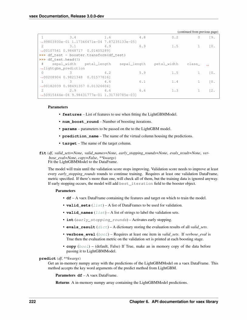
vaex Documentation, Release 3.0.0-dev
(continued from previous page)
1 3.4 1.6 4.8 0.2 0 [9.→˓99803930e-01 1.17346471e-04 7.87235133e-05]2 3.1 4.9 6.9 1.5 1 [0.→˓00107541 0.9848717 0.01405289]>>> df_test = booster.transform(df_test)>>> df_test.head(3)# sepal_width petal_length sepal_length petal_width class_→˓lightgbm_prediction0 3 4.2 5.9 1.5 1 [0.→˓00208904 0.9821348 0.01577616]1 3 4.6 6.1 1.4 1 [0.→˓00182039 0.98491357 0.01326604]2 2.9 4.6 6.6 1.3 1 [2.→˓50915444e-04 9.98431777e-01 1.31730785e-03]
Parameters
• features – List of features to use when fitting the LightGBMModel.
• num_boost_round – Number of boosting iterations.
• params – parameters to be passed on the to the LightGBM model.
• prediction_name – The name of the virtual column housing the predictions.
• target – The name of the target column.
fit(df, valid_sets=None, valid_names=None, early_stopping_rounds=None, evals_result=None, ver-bose_eval=None, copy=False, **kwargs)Fit the LightGBMModel to the DataFrame.
The model will train until the validation score stops improving. Validation score needs to improve at leastevery early_stopping_rounds rounds to continue training. Requires at least one validation DataFrame,metric specified. If there’s more than one, will check all of them, but the training data is ignored anyway.If early stopping occurs, the model will add best_iteration field to the booster object.
Parameters
• df – A vaex DataFrame containing the features and target on which to train the model.
• valid_sets (list) – A list of DataFrames to be used for validation.
• valid_names (list) – A list of strings to label the validation sets.
• int (early_stopping_rounds) – Activates early stopping.
• evals_result (dict) – A dictionary storing the evaluation results of all valid_sets.
• verbose_eval (bool) – Requires at least one item in valid_sets. If verbose_eval isTrue then the evaluation metric on the validation set is printed at each boosting stage.
• copy (bool) – (default, False) If True, make an in memory copy of the data beforepassing it to LightGBMModel.
predict(df, **kwargs)Get an in-memory numpy array with the predictions of the LightGBMModel on a vaex DataFrame. Thismethod accepts the key word arguments of the predict method from LightGBM.
Parameters df – A vaex DataFrame.
Returns A in-memory numpy array containing the LightGBMModel predictions.
222 Chapter 6. API documentation for vaex library

vaex Documentation, Release 3.0.0-dev
Return type numpy.array
transform(df)Transform a DataFrame such that it contains the predictions of the LightGBMModel in form of a virtualcolumn.
Parameters df – A vaex DataFrame.
Return copy A shallow copy of the DataFrame that includes the LightGBMModel prediction asa virtual column.
Return type DataFrame
class vaex.ml.xgboost.XGBoostModel(features=traitlets.Undefined, num_boost_round=0,params=traitlets.Undefined, predic-tion_name=’xgboost_prediction’, target=”)
Bases: vaex.ml.state.HasState
The XGBoost algorithm.
XGBoost is an optimized distributed gradient boosting library designed to be highly efficient, flexible andportable. It implements machine learning algorithms under the Gradient Boosting framework. XGBoost pro-vides a parallel tree boosting (also known as GBDT, GBM) that solves many data science problems in a fast andaccurate way. (https://github.com/dmlc/xgboost)
Example:
>>> import vaex>>> import vaex.ml.xgboost>>> df = vaex.ml.datasets.load_iris()>>> features = ['sepal_width', 'petal_length', 'sepal_length', 'petal_width']>>> df_train, df_test = df.ml.train_test_split()>>> params = {
'max_depth': 5,'learning_rate': 0.1,'objective': 'multi:softmax','num_class': 3,'subsample': 0.80,'colsample_bytree': 0.80,'silent': 1}
>>> booster = vaex.ml.xgboost.XGBoostModel(features=features, target='class_',→˓num_boost_round=100, params=params)>>> booster.fit(df_train)>>> df_train = booster.transform(df_train)>>> df_train.head(3)# sepal_length sepal_width petal_length petal_width class_→˓xgboost_prediction0 5.4 3 4.5 1.5 1→˓ 11 4.8 3.4 1.6 0.2 0→˓ 02 6.9 3.1 4.9 1.5 1→˓ 1>>> df_test = booster.transform(df_test)>>> df_test.head(3)# sepal_length sepal_width petal_length petal_width class_→˓xgboost_prediction0 5.9 3 4.2 1.5 1→˓ 11 6.1 3 4.6 1.4 1→˓ 1
(continues on next page)
6.4. Machine learning with vaex.ml 223

vaex Documentation, Release 3.0.0-dev
(continued from previous page)
2 6.6 2.9 4.6 1.3 1→˓ 1
Parameters
• features – List of features to use when fitting the XGBoostModel.
• num_boost_round – Number of boosting iterations.
• params – A dictionary of parameters to be passed on to the XGBoost model.
• prediction_name – The name of the virtual column housing the predictions.
• target – The name of the target column.
fit(df, evals=(), early_stopping_rounds=None, evals_result=None, verbose_eval=False, **kwargs)Fit the XGBoost model given a DataFrame.
This method accepts all key word arguments for the xgboost.train method.
Parameters
• df – A vaex DataFrame containing the features and target on which to train the model.
• evals – A list of pairs (DataFrame, string). List of items to be evaluated during training,this allows user to watch performance on the validation set.
• early_stopping_rounds (int) – Activates early stopping. Validation error needsto decrease at least every early_stopping_rounds round(s) to continue training. Requiresat least one item in evals. If there’s more than one, will use the last. Returns the modelfrom the last iteration (not the best one).
• evals_result (dict) – A dictionary storing the evaluation results of all the items inevals.
• verbose_eval (bool) – Requires at least one item in evals. If verbose_eval is Truethen the evaluation metric on the validation set is printed at each boosting stage.
predict(df, **kwargs)Provided a vaex DataFrame, get an in-memory numpy array with the predictions from the XGBoost model.This method accepts the key word arguments of the predict method from XGBoost.
Returns A in-memory numpy array containing the XGBoostModel predictions.
Return type numpy.array
transform(df)Transform a DataFrame such that it contains the predictions of the XGBoostModel in form of a virtualcolumn.
Parameters df – A vaex DataFrame. It should have the same columns as the DataFrame usedto train the model.
Return copy A shallow copy of the DataFrame that includes the XGBoostModel prediction asa virtual column.
Return type DataFrame
224 Chapter 6. API documentation for vaex library

vaex Documentation, Release 3.0.0-dev
6.4.5 Incubator/experimental
These models are in the incubator phase and may disappear in the future
class vaex.ml.incubator.annoy.ANNOYModel(features=traitlets.Undefined, metric=’euclidean’,n_neighbours=10, n_trees=10, predci-tion_name=’annoy_prediction’, predic-tion_name=’annoy_prediction’, search_k=-1)
Bases: vaex.ml.state.HasState
Parameters
• features – List of features to use.
• metric – Metric to use for distance calculations
• n_neighbours – Now many neighbours
• n_trees – Number of trees to build.
• predcition_name – Output column name for the neighbours when transforming aDataFrame
• prediction_name – Output column name for the neighbours when transforming aDataFrame
• search_k – Jovan?
6.4. Machine learning with vaex.ml 225

vaex Documentation, Release 3.0.0-dev
226 Chapter 6. API documentation for vaex library

CHAPTER 7
Datasets to download
Here we list a few datasets, that might be interesting to explore with vaex
7.1 New york taxi dataset
See for instance Analyzing 1.1 Billion NYC Taxi and Uber Trips, with a Vengeance for some ideas.
• Year: 2015 - 146 million rows - 23GB
• Year 2009-2015 - 1 billion rows - 135GB
[2]: import vaex
[12]: df = vaex.open("/Users/users/breddels/.vaex/data/nyc_taxi/nyc_taxi2015.hdf5")df.plot(df.col.pickup_longitude, df.col.pickup_latitude, f="log1p", show=True, limits=→˓"96%");
227

vaex Documentation, Release 3.0.0-dev
7.2 SDSS - dereddened
Only: ra, dec, g, r, g_r (deredenned using Schlegel maps).
The original query at SDSS archive was (although split in small parts):
SELECT ra, dec, g, r from PhotoObjAll WHERE type = 6 and clean = 1 and r>=10.0 and r→˓<23.5;
• 162 million rows - 10GB
[22]: sdss = vaex.open("/Users/maartenbreddels/vaex/data/sdss/sdss_dereddened.hdf5")sdss.healpix_plot(sdss.col.healpix, show=True, f="log", healpix_max_level=9, healpix_→˓level=9,
healpix_input='galactic', healpix_output='galactic', rotation=(0,45))
228 Chapter 7. Datasets to download
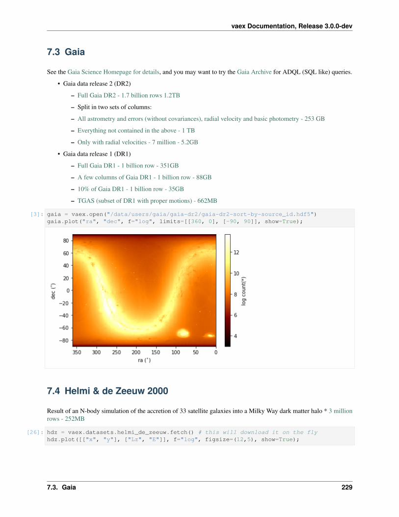
vaex Documentation, Release 3.0.0-dev
7.3 Gaia
See the Gaia Science Homepage for details, and you may want to try the Gaia Archive for ADQL (SQL like) queries.
• Gaia data release 2 (DR2)
– Full Gaia DR2 - 1.7 billion rows 1.2TB
– Split in two sets of columns:
– All astrometry and errors (without covariances), radial velocity and basic photometry - 253 GB
– Everything not contained in the above - 1 TB
– Only with radial velocities - 7 million - 5.2GB
• Gaia data release 1 (DR1)
– Full Gaia DR1 - 1 billion row - 351GB
– A few columns of Gaia DR1 - 1 billion row - 88GB
– 10% of Gaia DR1 - 1 billion row - 35GB
– TGAS (subset of DR1 with proper motions) - 662MB
[3]: gaia = vaex.open("/data/users/gaia/gaia-dr2/gaia-dr2-sort-by-source_id.hdf5")gaia.plot("ra", "dec", f="log", limits=[[360, 0], [-90, 90]], show=True);
7.4 Helmi & de Zeeuw 2000
Result of an N-body simulation of the accretion of 33 satellite galaxies into a Milky Way dark matter halo * 3 millionrows - 252MB
[26]: hdz = vaex.datasets.helmi_de_zeeuw.fetch() # this will download it on the flyhdz.plot([["x", "y"], ["Lz", "E"]], f="log", figsize=(12,5), show=True);
7.3. Gaia 229

vaex Documentation, Release 3.0.0-dev
230 Chapter 7. Datasets to download

CHAPTER 8
Frequently Asked Questions
8.1 I have a massive CSV file which I can not fit all into memory atone time. How do I convert it to HDF5?
Such an operation is a one-liner in Vaex:
df = vaex.from_csv('./my_data/my_big_file.csv', convert=True, chunk_size=5_000_000)
When the above line is executed, Vaex will read the CSV in chunks, and convert each chunk to a temporary HDF5 fileon disk. All temporary will files are then concatenated into a single HDF5, and the temporary files deleted. The sizeof the individual chunks to be read can be specified via the chunk_size argument.
For more information on importing and exporting data with Vaex, please refer to please refer to the I/O example page.
8.2 Why can’t I open a HDF5 file that was exported from a pandasDataFrame using .to_hdf?
When one uses the pandas .to_hdf method, the output HDF5 file has a row based format. Vaex on the otherhand expects column based HDF5 files. This allows for more efficient reading of data columns, which is much morecommonly required for data science applications.
One can easily export a pandas DataFrame to a vaex friendly HDF5 file:
vaex_df = vaex.from_pandas(pandas_df, copy_index=False)vaex_df.export_hdf5('my_data.hdf5')
231

vaex Documentation, Release 3.0.0-dev
232 Chapter 8. Frequently Asked Questions

CHAPTER 9
What is Vaex?
Vaex is a python library for lazy Out-of-Core DataFrames (similar to Pandas), to visualize and explore big tabulardatasets. It can calculate statistics such as mean, sum, count, standard deviation etc, on an N-dimensional grid upto a billion (109) objects/rows per second. Visualization is done using histograms, density plots and 3d volumerendering, allowing interactive exploration of big data. Vaex uses memory mapping, a zero memory copy policy, andlazy computations for best performance (no memory wasted).
9.1 Why vaex
• Performance: works with huge tabular data, processes 109 rows/second
• Lazy / Virtual columns: compute on the fly, without wasting ram
• Memory efficient no memory copies when doing filtering/selections/subsets.
• Visualization: directly supported, a one-liner is often enough.
• User friendly API: you will only need to deal with the DataFrame object, and tab completion + docstring willhelp you out: ds.mean<tab>, feels very similar to Pandas.
• Lean: separated into multiple packages
– vaex-core: DataFrame and core algorithms, takes numpy arrays as input columns.
– vaex-hdf5: Provides memory mapped numpy arrays to a DataFrame.
– vaex-arrow: Arrow support for cross language data sharing.
– vaex-viz: Visualization based on matplotlib.
– vaex-jupyter: Interactive visualization based on Jupyter widgets / ipywidgets, bqplot, ipyvolume andipyleaflet.
– vaex-astro: Astronomy related transformations and FITS file support.
– vaex-server: Provides a server to access a DataFrame remotely.
233

vaex Documentation, Release 3.0.0-dev
– vaex-distributed: (Proof of concept) combined multiple servers / cluster into a single DataFramefor distributed computations.
– vaex-qt: Program written using Qt GUI.
– vaex: Meta package that installs all of the above.
– vaex-ml: Machine learning
• Jupyter integration: vaex-jupyter will give you interactive visualization and selection in the Jupyter notebookand Jupyter lab.
234 Chapter 9. What is Vaex?

CHAPTER 10
Installation
Using conda:
• conda install -c conda-forge vaex
Using pip:
• pip install --upgrade vaex
Or read the detailed instructions
10.1 Getting started
We assume that you have installed vaex, and are running a Jupyter notebook server. We start by importing vaex andasking it to give us an example dataset.
[1]: import vaexdf = vaex.example() # open the example dataset provided with vaex
Instead, you can download some larger datasets, or read in your csv file.
[2]: df # will pretty print the DataFrame
[2]: # x y z vx vy vz→˓ E L Lz FeH0 -0.777470767 2.10626292 1.93743467 53.276722 288.386047 -95.→˓2649078 -121238.171875 831.0799560546875 -336.426513671875 -2.→˓3092276091645181 3.77427316 2.23387194 3.76209331 252.810791 -69.9498444 -56.→˓3121033 -100819.9140625 1435.1839599609375 -828.7567749023438 -1.→˓7887354915912292 1.3757627 -6.3283844 2.63250017 96.276474 226.440201 -34.→˓7527161 -100559.9609375 1039.2989501953125 920.802490234375 -0.→˓76181090224787983 -7.06737804 1.31737781 -6.10543537 204.968842 -205.679016 -58.→˓9777031 -70174.8515625 2441.724853515625 1183.5899658203125 -1.→˓5208778422936413
(continues on next page)
235

vaex Documentation, Release 3.0.0-dev
(continued from previous page)
4 0.243441463 -0.822781682 -0.206593871 -311.742371 -238.41217 186.→˓824127 -144138.75 374.8164367675781 -314.5353088378906 -2.→˓655341358427361... ... ... ... ... ... ...→˓ ... ... ... ...329,995 3.76883793 4.66251659 -4.42904139 107.432999 -2.13771296 17.→˓5130272 -119687.3203125 746.8833618164062 -508.96484375 -1.→˓6499842518381402329,996 9.17409325 -8.87091351 -8.61707687 32.0 108.089264 179.→˓060638 -68933.8046875 2395.633056640625 1275.490234375 -1.→˓4336036247720836329,997 -1.14041007 -8.4957695 2.25749826 8.46711349 -38.2765236 -127.→˓541473 -112580.359375 1182.436279296875 115.58557891845703 -1.→˓9306227597361942329,998 -14.2985935 -5.51750422 -8.65472317 110.221558 -31.3925591 86.→˓2726822 -74862.90625 1324.5926513671875 1057.017333984375 -1.→˓225019818838568329,999 10.5450506 -8.86106777 -4.65835428 -2.10541415 -27.6108856 3.→˓80799961 -95361.765625 351.0955505371094 -309.81439208984375 -2.→˓5689636894079477
Using ‘square brackets[] <api.rst#vaex.dataframe.DataFrame.__getitem__>‘__, we can easily filter or get differ-ent views on the DataFrame.
[3]: df_negative = df[df.x < 0] # easily filter your DataFrame, without making a copydf_negative[:5][['x', 'y']] # take the first five rows, and only the 'x' and 'y'→˓column (no memory copy!)
[3]: # x y0 -0.777471 2.106261 -7.06738 1.317382 -5.17174 7.829153 -15.9539 5.771264 -12.3995 13.9182
When dealing with huge datasets, say a billion rows (109), computations with the data can waste memory, up to 8GB for a new column. Instead, vaex uses lazy computation, storing only a representation of the computation, andcomputations are done on the fly when needed. You can just use many of the numpy functions, as if it was a normalarray.
[4]: import numpy as np# creates an expression (nothing is computed)some_expression = df.x + df.zsome_expression # for convenience, we print out some values
[4]: <vaex.expression.Expression(expressions='(x + z)')> instance at 0x118f71550 values=[1.→˓159963903, 7.53636647, 4.00826287, -13.17281341, 0.036847591999999985 ... (total→˓330000 values) ... -0.66020346, 0.5570163800000003, 1.1170881900000003, -22.→˓95331667, 5.8866963199999995]
These expressions can be added to a DataFrame, creating what we call a virtual column. These virtual columns aresimilar to normal columns, except they do not waste memory.
[5]: df['r'] = some_expression # add a (virtual) column that will be computed on the flydf.mean(df.x), df.mean(df.r) # calculate statistics on normal and virtual columns
[5]: (-0.06713149126400597, -0.0501732470530304)
236 Chapter 10. Installation
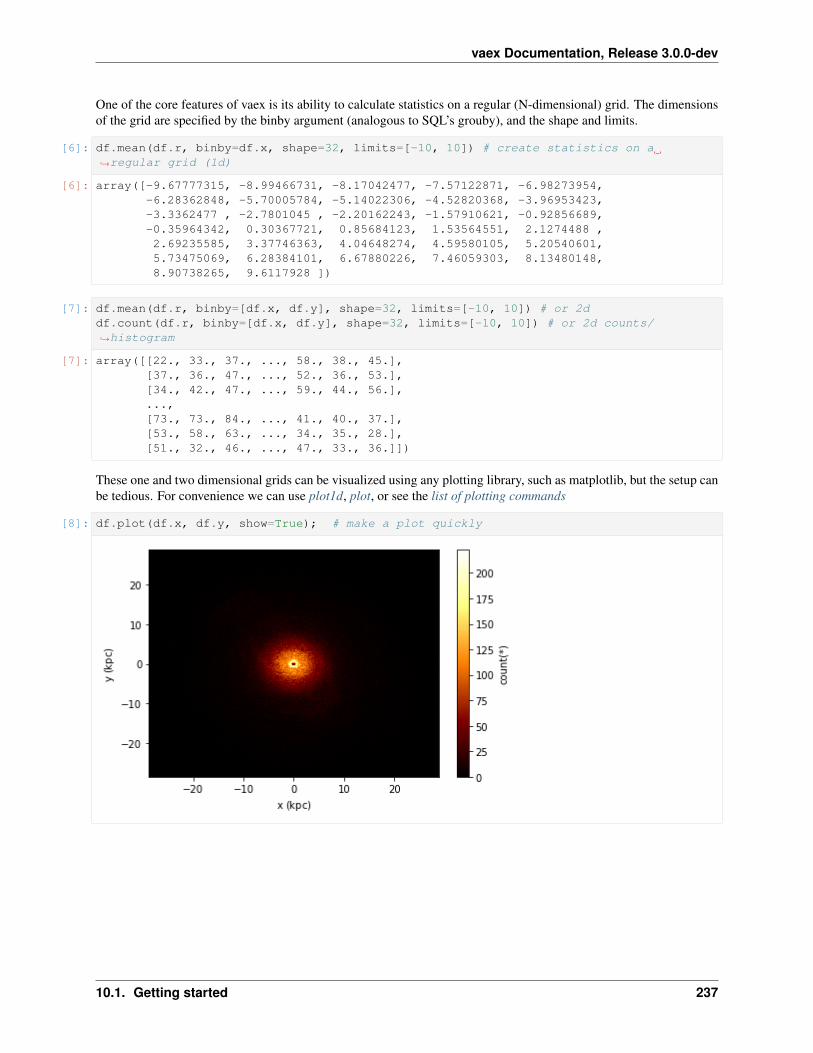
vaex Documentation, Release 3.0.0-dev
One of the core features of vaex is its ability to calculate statistics on a regular (N-dimensional) grid. The dimensionsof the grid are specified by the binby argument (analogous to SQL’s grouby), and the shape and limits.
[6]: df.mean(df.r, binby=df.x, shape=32, limits=[-10, 10]) # create statistics on a→˓regular grid (1d)
[6]: array([-9.67777315, -8.99466731, -8.17042477, -7.57122871, -6.98273954,-6.28362848, -5.70005784, -5.14022306, -4.52820368, -3.96953423,-3.3362477 , -2.7801045 , -2.20162243, -1.57910621, -0.92856689,-0.35964342, 0.30367721, 0.85684123, 1.53564551, 2.1274488 ,2.69235585, 3.37746363, 4.04648274, 4.59580105, 5.20540601,5.73475069, 6.28384101, 6.67880226, 7.46059303, 8.13480148,8.90738265, 9.6117928 ])
[7]: df.mean(df.r, binby=[df.x, df.y], shape=32, limits=[-10, 10]) # or 2ddf.count(df.r, binby=[df.x, df.y], shape=32, limits=[-10, 10]) # or 2d counts/→˓histogram
[7]: array([[22., 33., 37., ..., 58., 38., 45.],[37., 36., 47., ..., 52., 36., 53.],[34., 42., 47., ..., 59., 44., 56.],...,[73., 73., 84., ..., 41., 40., 37.],[53., 58., 63., ..., 34., 35., 28.],[51., 32., 46., ..., 47., 33., 36.]])
These one and two dimensional grids can be visualized using any plotting library, such as matplotlib, but the setup canbe tedious. For convenience we can use plot1d, plot, or see the list of plotting commands
[8]: df.plot(df.x, df.y, show=True); # make a plot quickly
10.1. Getting started 237

vaex Documentation, Release 3.0.0-dev
238 Chapter 10. Installation

CHAPTER 11
Continue
Continue the tutorial here or check the examples
239

vaex Documentation, Release 3.0.0-dev
240 Chapter 11. Continue

Python Module Index
vvaex, 112vaex.agg, 169vaex.ml.sklearn, 206vaex.stat, 168
241

vaex Documentation, Release 3.0.0-dev
242 Python Module Index

Index
Symbols__abs__() (vaex.expression.Expression method), 162__array__() (vaex.dataframe.DataFrameLocal
method), 156__call__() (vaex.dataframe.DataFrameLocal
method), 157__delitem__() (vaex.dataframe.DataFrame
method), 118__getitem__() (vaex.dataframe.DataFrame
method), 118__init__() (vaex.dataframe.DataFrame method), 118__init__() (vaex.dataframe.DataFrameLocal
method), 157__init__() (vaex.expression.DateTime method), 191__init__() (vaex.expression.Expression method), 162__init__() (vaex.expression.StringOperations
method), 170__init__() (vaex.expression.StringOperationsPandas
method), 189__init__() (vaex.expression.TimeDelta method), 198__init__() (vaex.geo.DataFrameAccessorGeo
method), 200__init__() (vaex.graphql.DataFrameAccessorGraphQL
method), 206__iter__() (vaex.dataframe.DataFrame method), 118__len__() (vaex.dataframe.DataFrame method), 118__repr__() (vaex.dataframe.DataFrame method), 118__repr__() (vaex.expression.Expression method), 162__setitem__() (vaex.dataframe.DataFrame
method), 118__str__() (vaex.dataframe.DataFrame method), 118__str__() (vaex.expression.Expression method), 162__weakref__ (vaex.dataframe.DataFrame attribute),
118__weakref__ (vaex.expression.DateTime attribute),
191__weakref__ (vaex.expression.Expression attribute),
163__weakref__ (vaex.expression.StringOperations at-
tribute), 170__weakref__ (vaex.expression.StringOperationsPandas
attribute), 189__weakref__ (vaex.expression.TimeDelta attribute),
198__weakref__ (vaex.geo.DataFrameAccessorGeo at-
tribute), 200__weakref__ (vaex.graphql.DataFrameAccessorGraphQL
attribute), 206
Aabs() (vaex.expression.Expression method), 163add_column() (vaex.dataframe.DataFrame method),
118add_variable() (vaex.dataframe.DataFrame
method), 118add_virtual_column()
(vaex.dataframe.DataFrame method), 119AggregatorDescriptorMean (class in vaex.agg),
169AggregatorDescriptorMulti (class in vaex.agg),
169AggregatorDescriptorStd (class in vaex.agg),
169AggregatorDescriptorVar (class in vaex.agg),
169ANNOYModel (class in vaex.ml.incubator.annoy), 225app() (in module vaex), 117apply() (vaex.dataframe.DataFrame method), 119apply() (vaex.expression.Expression method), 163arccos() (vaex.expression.Expression method), 163arccosh() (vaex.expression.Expression method), 163arcsin() (vaex.expression.Expression method), 163arcsinh() (vaex.expression.Expression method), 163arctan() (vaex.expression.Expression method), 163arctan2() (vaex.expression.Expression method), 163arctanh() (vaex.expression.Expression method), 163ast (vaex.expression.Expression attribute), 163
243

vaex Documentation, Release 3.0.0-dev
Bbatch_size (vaex.ml.sklearn.IncrementalPredictor at-
tribute), 208BayesianTargetEncoder (class in
vaex.ml.transformations), 219bearing() (vaex.geo.DataFrameAccessorGeo
method), 200binby() (vaex.dataframe.DataFrameLocal method),
157byte_length() (vaex.expression.StringOperations
method), 170byte_length() (vaex.expression.StringOperationsPandas
method), 189byte_size() (vaex.dataframe.DataFrame method),
119
Ccalculate() (vaex.stat.Expression method), 168capitalize() (vaex.expression.StringOperations
method), 170capitalize() (vaex.expression.StringOperationsPandas
method), 189cartesian2spherical()
(vaex.geo.DataFrameAccessorGeo method),200
cartesian_to_polar()(vaex.geo.DataFrameAccessorGeo method),201
cat() (vaex.dataframe.DataFrame method), 119cat() (vaex.expression.StringOperations method), 171cat() (vaex.expression.StringOperationsPandas
method), 189categorize() (vaex.dataframe.DataFrameLocal
method), 157center() (vaex.expression.StringOperations method),
171center() (vaex.expression.StringOperationsPandas
method), 189clip() (vaex.expression.Expression method), 164close_files() (vaex.dataframe.DataFrame
method), 120col (vaex.dataframe.DataFrame attribute), 120column_count() (vaex.dataframe.DataFrame
method), 120combinations() (vaex.dataframe.DataFrame
method), 120compare() (vaex.dataframe.DataFrameLocal method),
157concat() (vaex.dataframe.DataFrameLocal method),
157contains() (vaex.expression.StringOperations
method), 172contains() (vaex.expression.StringOperationsPandas
method), 189
copy() (vaex.expression.Expression method), 164correlation() (in module vaex.stat), 168correlation() (vaex.dataframe.DataFrame
method), 120cos() (vaex.expression.Expression method), 164cosh() (vaex.expression.Expression method), 164count() (in module vaex.agg), 169count() (in module vaex.stat), 168count() (vaex.dataframe.DataFrame method), 121count() (vaex.expression.Expression method), 164count() (vaex.expression.StringOperations method),
173count() (vaex.expression.StringOperationsPandas
method), 189countmissing() (vaex.expression.Expression
method), 164countna() (vaex.expression.Expression method), 164countnan() (vaex.expression.Expression method), 164cov() (vaex.dataframe.DataFrame method), 122covar() (in module vaex.stat), 169covar() (vaex.dataframe.DataFrame method), 122CycleTransformer (class in
vaex.ml.transformations), 218
Ddata (vaex.dataframe.DataFrameLocal attribute), 157data_type() (vaex.dataframe.DataFrame method),
123data_type() (vaex.expression.Expression method),
164DataFrame (class in vaex.dataframe), 117DataFrameAccessorGeo (class in vaex.geo), 200DataFrameAccessorGraphQL (class in
vaex.graphql), 206DataFrameLocal (class in vaex.dataframe), 156DateTime (class in vaex.expression), 191day (vaex.expression.DateTime attribute), 191day_name (vaex.expression.DateTime attribute), 192dayofweek (vaex.expression.DateTime attribute), 192dayofyear (vaex.expression.DateTime attribute), 192days (vaex.expression.TimeDelta attribute), 198deg2rad() (vaex.expression.Expression method), 164delayed() (in module vaex), 117delete_variable() (vaex.dataframe.DataFrame
method), 123delete_virtual_column()
(vaex.dataframe.DataFrame method), 123describe() (vaex.dataframe.DataFrame method), 123digitize() (vaex.expression.Expression method), 164drop() (vaex.dataframe.DataFrame method), 124drop_filter() (vaex.dataframe.DataFrame
method), 124dropmissing() (vaex.dataframe.DataFrame
method), 124
244 Index

vaex Documentation, Release 3.0.0-dev
dropna() (vaex.dataframe.DataFrame method), 124dropnan() (vaex.dataframe.DataFrame method), 124dt (vaex.expression.Expression attribute), 164dtypes (vaex.dataframe.DataFrame attribute), 124
Eendswith() (vaex.expression.StringOperations
method), 173endswith() (vaex.expression.StringOperationsPandas
method), 189equals() (vaex.expression.StringOperations method),
174equals() (vaex.expression.StringOperationsPandas
method), 189evaluate() (vaex.dataframe.DataFrame method), 124evaluate_iterator() (vaex.dataframe.DataFrame
method), 125evaluate_variable() (vaex.dataframe.DataFrame
method), 125example() (in module vaex), 117execute() (vaex.dataframe.DataFrame method), 125execute() (vaex.graphql.DataFrameAccessorGraphQL
method), 206exp() (vaex.expression.Expression method), 164expand() (vaex.expression.Expression method), 164expm1() (vaex.expression.Expression method), 164export() (vaex.dataframe.DataFrameLocal method),
157export_arrow() (vaex.dataframe.DataFrameLocal
method), 158export_csv() (vaex.dataframe.DataFrameLocal
method), 158export_fits() (vaex.dataframe.DataFrameLocal
method), 159export_hdf5() (vaex.dataframe.DataFrameLocal
method), 159export_parquet() (vaex.dataframe.DataFrameLocal
method), 159Expression (class in vaex.expression), 162Expression (class in vaex.stat), 168extract() (vaex.dataframe.DataFrame method), 125
Ffeatures (vaex.ml.sklearn.IncrementalPredictor at-
tribute), 208features (vaex.ml.sklearn.Predictor attribute), 209fillmissing() (vaex.expression.Expression
method), 164fillna() (vaex.dataframe.DataFrame method), 125fillna() (vaex.expression.Expression method), 165fillnan() (vaex.expression.Expression method), 165filter() (vaex.dataframe.DataFrame method), 126find() (vaex.expression.StringOperations method),
174
find() (vaex.expression.StringOperationsPandasmethod), 189
first() (in module vaex.agg), 169first() (vaex.dataframe.DataFrame method), 127fit() (vaex.ml.cluster.KMeans method), 211fit() (vaex.ml.lightgbm.LightGBMModel method), 222fit() (vaex.ml.sklearn.IncrementalPredictor method),
208fit() (vaex.ml.sklearn.Predictor method), 209fit() (vaex.ml.transformations.BayesianTargetEncoder
method), 220fit() (vaex.ml.transformations.CycleTransformer
method), 219fit() (vaex.ml.transformations.FrequencyEncoder
method), 213fit() (vaex.ml.transformations.LabelEncoder method),
213fit() (vaex.ml.transformations.MaxAbsScaler
method), 214fit() (vaex.ml.transformations.MinMaxScaler
method), 215fit() (vaex.ml.transformations.OneHotEncoder
method), 216fit() (vaex.ml.transformations.PCA method), 217fit() (vaex.ml.transformations.RobustScaler method),
217fit() (vaex.ml.transformations.StandardScaler
method), 218fit() (vaex.ml.transformations.WeightOfEvidenceEncoder
method), 220fit() (vaex.ml.xgboost.XGBoostModel method), 224format() (vaex.expression.Expression method), 165FrequencyEncoder (class in
vaex.ml.transformations), 212from_arrays() (in module vaex), 114from_arrow_table() (in module vaex), 115from_ascii() (in module vaex), 115from_astropy_table() (in module vaex), 116from_csv() (in module vaex), 115from_dict() (in module vaex), 114from_items() (in module vaex), 114from_pandas() (in module vaex), 116from_samp() (in module vaex), 116
Gget() (vaex.expression.StringOperations method), 175get() (vaex.expression.StringOperationsPandas
method), 190get_active_fraction()
(vaex.dataframe.DataFrame method), 128get_column_names() (vaex.dataframe.DataFrame
method), 128get_current_row() (vaex.dataframe.DataFrame
method), 128
Index 245

vaex Documentation, Release 3.0.0-dev
get_names() (vaex.dataframe.DataFrame method),128
get_private_dir() (vaex.dataframe.DataFramemethod), 128
get_selection() (vaex.dataframe.DataFramemethod), 128
get_variable() (vaex.dataframe.DataFramemethod), 129
groupby() (vaex.dataframe.DataFrameLocal method),160
Hhas_current_row() (vaex.dataframe.DataFrame
method), 129has_selection() (vaex.dataframe.DataFrame
method), 129head() (vaex.dataframe.DataFrame method), 129head_and_tail_print()
(vaex.dataframe.DataFrame method), 129healpix_count() (vaex.dataframe.DataFrame
method), 129healpix_plot() (vaex.dataframe.DataFrame
method), 129hour (vaex.expression.DateTime attribute), 193
IIncrementalPredictor (class in vaex.ml.sklearn),
206index() (vaex.expression.StringOperations method),
175index() (vaex.expression.StringOperationsPandas
method), 190inside_polygon() (vaex.geo.DataFrameAccessorGeo
method), 201inside_polygons()
(vaex.geo.DataFrameAccessorGeo method),201
inside_which_polygon()(vaex.geo.DataFrameAccessorGeo method),202
inside_which_polygons()(vaex.geo.DataFrameAccessorGeo method),202
is_category() (vaex.dataframe.DataFramemethod), 130
is_leap_year (vaex.expression.DateTime attribute),193
is_local() (vaex.dataframe.DataFrame method), 130is_local() (vaex.dataframe.DataFrameLocal
method), 161is_masked() (vaex.dataframe.DataFrame method),
130isalnum() (vaex.expression.StringOperations
method), 176
isalnum() (vaex.expression.StringOperationsPandasmethod), 190
isalpha() (vaex.expression.StringOperationsmethod), 177
isalpha() (vaex.expression.StringOperationsPandasmethod), 190
isdigit() (vaex.expression.StringOperationsmethod), 177
isdigit() (vaex.expression.StringOperationsPandasmethod), 190
isfinite() (vaex.expression.Expression method), 165isin() (vaex.expression.Expression method), 165islower() (vaex.expression.StringOperations
method), 178islower() (vaex.expression.StringOperationsPandas
method), 190ismissing() (vaex.expression.Expression method),
165isna() (vaex.expression.Expression method), 165isnan() (vaex.expression.Expression method), 165isspace() (vaex.expression.StringOperations
method), 178isspace() (vaex.expression.StringOperationsPandas
method), 190isupper() (vaex.expression.StringOperations
method), 179isupper() (vaex.expression.StringOperationsPandas
method), 190
Jjoin() (vaex.dataframe.DataFrameLocal method), 161join() (vaex.expression.StringOperations method),
179join() (vaex.expression.StringOperationsPandas
method), 190
KKMeans (class in vaex.ml.cluster), 210
Llabel_encode() (vaex.dataframe.DataFrameLocal
method), 162LabelEncoder (class in vaex.ml.transformations), 213len() (vaex.expression.StringOperations method), 179len() (vaex.expression.StringOperationsPandas
method), 190length() (vaex.dataframe.DataFrameLocal method),
162length_original() (vaex.dataframe.DataFrame
method), 130length_unfiltered() (vaex.dataframe.DataFrame
method), 130LightGBMModel (class in vaex.ml.lightgbm), 221limits() (vaex.dataframe.DataFrame method), 130
246 Index

vaex Documentation, Release 3.0.0-dev
limits_percentage() (vaex.dataframe.DataFramemethod), 131
ljust() (vaex.expression.StringOperations method),180
ljust() (vaex.expression.StringOperationsPandasmethod), 190
log() (vaex.expression.Expression method), 165log10() (vaex.expression.Expression method), 165log1p() (vaex.expression.Expression method), 165lower() (vaex.expression.StringOperations method),
180lower() (vaex.expression.StringOperationsPandas
method), 190lstrip() (vaex.expression.StringOperations method),
181lstrip() (vaex.expression.StringOperationsPandas
method), 190
Mmap() (vaex.expression.Expression method), 165masked (vaex.expression.Expression attribute), 166match() (vaex.expression.StringOperations method),
181match() (vaex.expression.StringOperationsPandas
method), 190materialize() (vaex.dataframe.DataFrame
method), 131max() (in module vaex.agg), 169max() (vaex.dataframe.DataFrame method), 132max() (vaex.expression.Expression method), 166MaxAbsScaler (class in vaex.ml.transformations), 214maximum() (vaex.expression.Expression method), 166mean() (in module vaex.agg), 169mean() (in module vaex.stat), 169mean() (vaex.dataframe.DataFrame method), 132mean() (vaex.expression.Expression method), 166median_approx() (vaex.dataframe.DataFrame
method), 133microseconds (vaex.expression.TimeDelta attribute),
198min() (in module vaex.agg), 169min() (vaex.dataframe.DataFrame method), 133min() (vaex.expression.Expression method), 166minimum() (vaex.expression.Expression method), 166minmax() (vaex.dataframe.DataFrame method), 134minmax() (vaex.expression.Expression method), 166MinMaxScaler (class in vaex.ml.transformations), 214minute (vaex.expression.DateTime attribute), 194mode() (vaex.dataframe.DataFrame method), 135model (vaex.ml.sklearn.IncrementalPredictor attribute),
208model (vaex.ml.sklearn.Predictor attribute), 210month (vaex.expression.DateTime attribute), 194month_name (vaex.expression.DateTime attribute), 195
mutual_information()(vaex.dataframe.DataFrame method), 135
Nnanoseconds (vaex.expression.TimeDelta attribute),
199nbytes (vaex.dataframe.DataFrame attribute), 136nop() (vaex.dataframe.DataFrame method), 136nop() (vaex.expression.Expression method), 166notna() (vaex.expression.Expression method), 166num_epochs (vaex.ml.sklearn.IncrementalPredictor at-
tribute), 208nunique() (in module vaex.agg), 169nunique() (vaex.expression.Expression method), 166
OOneHotEncoder (class in vaex.ml.transformations),
215open() (in module vaex), 113open_many() (in module vaex), 116ordinal_encode() (vaex.dataframe.DataFrameLocal
method), 162
Ppad() (vaex.expression.StringOperations method), 182pad() (vaex.expression.StringOperationsPandas
method), 190partial_fit_kwargs
(vaex.ml.sklearn.IncrementalPredictor at-tribute), 208
PCA (class in vaex.ml.transformations), 216percentile_approx() (vaex.dataframe.DataFrame
method), 136plot() (vaex.dataframe.DataFrame method), 136plot1d() (vaex.dataframe.DataFrame method), 138plot2d_contour() (vaex.dataframe.DataFrame
method), 139plot3d() (vaex.dataframe.DataFrame method), 140plot_bq() (vaex.dataframe.DataFrame method), 140plot_widget() (vaex.dataframe.DataFrame
method), 140predict() (vaex.ml.lightgbm.LightGBMModel
method), 222predict() (vaex.ml.sklearn.IncrementalPredictor
method), 208predict() (vaex.ml.sklearn.Predictor method), 210predict() (vaex.ml.xgboost.XGBoostModel method),
224prediction_name (vaex.ml.sklearn.IncrementalPredictor
attribute), 208prediction_name (vaex.ml.sklearn.Predictor at-
tribute), 210Predictor (class in vaex.ml.sklearn), 208
Index 247

vaex Documentation, Release 3.0.0-dev
project_aitoff() (vaex.geo.DataFrameAccessorGeomethod), 203
project_gnomic() (vaex.geo.DataFrameAccessorGeomethod), 204
propagate_uncertainties()(vaex.dataframe.DataFrame method), 140
Qquarter (vaex.expression.DateTime attribute), 195query() (vaex.graphql.DataFrameAccessorGraphQL
method), 206
Rrad2deg() (vaex.expression.Expression method), 167register_function() (in module vaex), 116remove_virtual_meta()
(vaex.dataframe.DataFrame method), 141rename() (vaex.dataframe.DataFrame method), 141repeat() (vaex.expression.StringOperations method),
182repeat() (vaex.expression.StringOperationsPandas
method), 190replace() (vaex.expression.StringOperations
method), 183replace() (vaex.expression.StringOperationsPandas
method), 190rfind() (vaex.expression.StringOperations method),
183rfind() (vaex.expression.StringOperationsPandas
method), 190rindex() (vaex.expression.StringOperations method),
184rindex() (vaex.expression.StringOperationsPandas
method), 190rjust() (vaex.expression.StringOperations method),
185rjust() (vaex.expression.StringOperationsPandas
method), 190RobustScaler (class in vaex.ml.transformations), 217rotation_2d() (vaex.geo.DataFrameAccessorGeo
method), 204rstrip() (vaex.expression.StringOperations method),
185rstrip() (vaex.expression.StringOperationsPandas
method), 190
Ssample() (vaex.dataframe.DataFrame method), 141scatter() (vaex.dataframe.DataFrame method), 142schema() (vaex.graphql.DataFrameAccessorGraphQL
method), 206searchsorted() (vaex.expression.Expression
method), 167second (vaex.expression.DateTime attribute), 196
seconds (vaex.expression.TimeDelta attribute), 199select() (vaex.dataframe.DataFrame method), 143select_box() (vaex.dataframe.DataFrame method),
143select_circle() (vaex.dataframe.DataFrame
method), 143select_ellipse() (vaex.dataframe.DataFrame
method), 143select_inverse() (vaex.dataframe.DataFrame
method), 144select_lasso() (vaex.dataframe.DataFrame
method), 144select_non_missing()
(vaex.dataframe.DataFrame method), 144select_nothing() (vaex.dataframe.DataFrame
method), 145select_rectangle() (vaex.dataframe.DataFrame
method), 145selected_length() (vaex.dataframe.DataFrame
method), 145selected_length()
(vaex.dataframe.DataFrameLocal method),162
selection_can_redo()(vaex.dataframe.DataFrame method), 145
selection_can_undo()(vaex.dataframe.DataFrame method), 145
selection_redo() (vaex.dataframe.DataFramemethod), 145
selection_undo() (vaex.dataframe.DataFramemethod), 145
serve() (vaex.graphql.DataFrameAccessorGraphQLmethod), 206
set_active_fraction()(vaex.dataframe.DataFrame method), 145
set_active_range() (vaex.dataframe.DataFramemethod), 145
set_current_row() (vaex.dataframe.DataFramemethod), 145
set_selection() (vaex.dataframe.DataFramemethod), 145
set_variable() (vaex.dataframe.DataFramemethod), 146
shallow_copy() (vaex.dataframe.DataFrameLocalmethod), 162
shuffle (vaex.ml.sklearn.IncrementalPredictor at-tribute), 208
sin() (vaex.expression.Expression method), 167sinc() (vaex.expression.Expression method), 167sinh() (vaex.expression.Expression method), 167SKLearnPredictor (class in vaex.ml.sklearn), 210slice() (vaex.expression.StringOperations method),
186slice() (vaex.expression.StringOperationsPandas
248 Index

vaex Documentation, Release 3.0.0-dev
method), 191sort() (vaex.dataframe.DataFrame method), 146spherical2cartesian()
(vaex.geo.DataFrameAccessorGeo method),204
split() (vaex.dataframe.DataFrame method), 147split() (vaex.expression.StringOperationsPandas
method), 191split_random() (vaex.dataframe.DataFrame
method), 147sqrt() (vaex.expression.Expression method), 167StandardScaler (class in vaex.ml.transformations),
218startswith() (vaex.expression.StringOperations
method), 186startswith() (vaex.expression.StringOperationsPandas
method), 191state_get() (vaex.dataframe.DataFrame method),
148state_load() (vaex.dataframe.DataFrame method),
148state_set() (vaex.dataframe.DataFrame method),
148state_write() (vaex.dataframe.DataFrame
method), 149std() (in module vaex.agg), 169std() (in module vaex.stat), 169std() (vaex.dataframe.DataFrame method), 150std() (vaex.expression.Expression method), 167str (vaex.expression.Expression attribute), 167str_pandas (vaex.expression.Expression attribute),
167strftime() (vaex.expression.DateTime method), 196StringOperations (class in vaex.expression), 170StringOperationsPandas (class in
vaex.expression), 189strip() (vaex.expression.StringOperations method),
187strip() (vaex.expression.StringOperationsPandas
method), 191sum() (in module vaex.agg), 169sum() (in module vaex.stat), 169sum() (vaex.dataframe.DataFrame method), 151sum() (vaex.expression.Expression method), 167
Ttail() (vaex.dataframe.DataFrame method), 151take() (vaex.dataframe.DataFrame method), 151tan() (vaex.expression.Expression method), 167tanh() (vaex.expression.Expression method), 167target (vaex.ml.sklearn.IncrementalPredictor at-
tribute), 208target (vaex.ml.sklearn.Predictor attribute), 210td (vaex.expression.Expression attribute), 167
TimeDelta (class in vaex.expression), 198title() (vaex.expression.StringOperations method),
187title() (vaex.expression.StringOperationsPandas
method), 191to_arrays() (vaex.dataframe.DataFrame method),
152to_arrow_table() (vaex.dataframe.DataFrame
method), 152to_astropy_table() (vaex.dataframe.DataFrame
method), 153to_copy() (vaex.dataframe.DataFrame method), 153to_dask_array() (vaex.dataframe.DataFrame
method), 153to_dict() (vaex.dataframe.DataFrame method), 153to_items() (vaex.dataframe.DataFrame method), 154to_numpy() (vaex.expression.Expression method), 167to_pandas_df() (vaex.dataframe.DataFrame
method), 154to_pandas_series() (vaex.expression.Expression
method), 167tolist() (vaex.expression.Expression method), 167total_seconds() (vaex.expression.TimeDelta
method), 200transform() (vaex.ml.cluster.KMeans method), 211transform() (vaex.ml.lightgbm.LightGBMModel
method), 223transform() (vaex.ml.sklearn.IncrementalPredictor
method), 208transform() (vaex.ml.sklearn.Predictor method), 210transform() (vaex.ml.transformations.BayesianTargetEncoder
method), 220transform() (vaex.ml.transformations.CycleTransformer
method), 219transform() (vaex.ml.transformations.FrequencyEncoder
method), 213transform() (vaex.ml.transformations.LabelEncoder
method), 213transform() (vaex.ml.transformations.MaxAbsScaler
method), 214transform() (vaex.ml.transformations.MinMaxScaler
method), 215transform() (vaex.ml.transformations.OneHotEncoder
method), 216transform() (vaex.ml.transformations.PCA method),
217transform() (vaex.ml.transformations.RobustScaler
method), 218transform() (vaex.ml.transformations.StandardScaler
method), 218transform() (vaex.ml.transformations.WeightOfEvidenceEncoder
method), 221transform() (vaex.ml.xgboost.XGBoostModel
method), 224
Index 249
vaex Documentation, Release 3.0.0-dev
transient (vaex.expression.Expression attribute), 167trim() (vaex.dataframe.DataFrame method), 155
Uucd_find() (vaex.dataframe.DataFrame method), 155unique() (vaex.expression.Expression method), 167unit() (vaex.dataframe.DataFrame method), 155upper() (vaex.expression.StringOperations method),
188upper() (vaex.expression.StringOperationsPandas
method), 191
Vvaex (module), 112vaex.agg (module), 169vaex.ml.sklearn (module), 206vaex.stat (module), 168validate_expression()
(vaex.dataframe.DataFrame method), 156value_counts() (vaex.expression.Expression
method), 168var() (in module vaex.agg), 170var() (vaex.dataframe.DataFrame method), 156var() (vaex.expression.Expression method), 168variables() (vaex.expression.Expression method),
168velocity_cartesian2polar()
(vaex.geo.DataFrameAccessorGeo method),204
velocity_cartesian2spherical()(vaex.geo.DataFrameAccessorGeo method),205
velocity_polar2cartesian()(vaex.geo.DataFrameAccessorGeo method),205
Wweekofyear (vaex.expression.DateTime attribute), 197WeightOfEvidenceEncoder (class in
vaex.ml.transformations), 220where() (vaex.expression.Expression method), 168
XXGBoostModel (class in vaex.ml.xgboost), 223
Yyear (vaex.expression.DateTime attribute), 197
Zzfill() (vaex.expression.StringOperations method),
188zfill() (vaex.expression.StringOperationsPandas
method), 191
250 Index