validating bayesian inference algorithms with simulation … procedure can be sped up further by...

Validating Bayesian InferenceAlgorithms with Simulation-BasedCalibrationSean Talts, Michael Betancourt, Daniel Simpson, Aki Vehtari, AndrewGelman

Abstract. Verifying the correctness of Bayesian computation is challeng-ing. This is especially true for complex models that are common in prac-tice, as these require sophisticated model implementations and algo-rithms. In this paper we introduce simulation-based calibration (SBC),a general procedure for validating inferences from Bayesian algorithmscapable of generating posterior samples. This procedure not only iden-tifies inaccurate computation and inconsistencies in model implemen-tations but also provides graphical summaries that can indicate thenature of the problems that arise. We argue that SBC is a critical partof a robust Bayesian workflow, as well as being a useful tool for thosedeveloping computational algorithms and statistical software.

1. INTRODUCTION

Powerful algorithms and computational resources are facilitating Bayesian modelingin an increasing range of applications. Conceptually, constructing a Bayesian analysis isstraightforward. We first define a joint distribution over the parameters, θ, and measure-ments, y, with the specification of a prior distribution and likelihood,

π(y, θ) = π(y | θ)π(θ).

Conditioning this joint distribution on an observation, y, yields a posterior distribution,

π(θ | y) ∝ π(y, θ),

ISERP, Columbia University, New York. (e-mail: [email protected]).Symplectomorphic LLC., New York. (e-mail: [email protected]). Department ofStatistical Sciences, University of Toronto, Toronto. (e-mail:[email protected]). Helsinki Institute for Information Technology HIIT,Department of Computer Science, Aalto University, Finland. (e-mail:[email protected]). Department of Statistics and Department of Political Science,Columbia University, New York. (e-mail: [email protected]).

1

arX

iv:1

804.

0678

8v1

[st

at.M

E]

18

Apr

201

8

mailto:[email protected]





2 S. TALTS ET AL.

that encodes information about the system being analyzed.Implementing this Bayesian inference in practice, however, can be computationally chal-

lenging when applied to large and structured datasets. We must make our model richenough to capture the relevant structure of the system being studied while simultaneouslybeing able to accurately work with the resulting posterior distribution. Unfortunately, everyalgorithm in computational statistics requires that the posterior distribution possesses cer-tain favorable properties in order to be successful. Consequently the overall performanceof an algorithm is sensitive to the details of the model and the observed data, and analgorithm that works well in one analysis can fail spectacularly in another.

As we move towards creating sophisticated, bespoke models with each analysis, we stressthe algorithms in our statistical toolbox. Moreover, the complexity of these models providesabundant opportunity for mistakes in their specification. We must verify both that ourcode is implementing the model we think it is and that our inference algorithm is able toperform the necessary computations accurately. While we always get some result from agiven algorithm, we have no idea how good it might be without some form of validation.

Fortunately, the structure of the Bayesian joint distribution allows for the validationof any Bayesian computational method capable of producing samples from the posteriordistribution, or an approximation thereof. This includes not only Monte Carlo methodsbut also deterministic methods that yield approximate posterior distributions amenable toexact sampling, such as integrated nested Laplace approximation (INLA) (Rue, Martinoand Chopin, 2009; Rue et al., 2017) and automatic differentiation variational inference(ADVI) (Kucukelbir et al., 2017). In this paper we introduce Simulation-Based Calibration(SBC), a generic and straightforward procedure for validating these algorithms within thescope of a given Bayesian joint distribution.

We begin with a discussion the natural self-consistency of samples from the Bayesianjoint distribution and previous validation methods that have exploited this behavior. Nextwe introduce the simulation-based calibration framework and examine the qualitative in-terpretation of the SBC output, how it identifies how the algorithm being validated mightbe failing, and how it can be incorporated into a robust Bayesian workflow. Finally, we con-sider some useful extensions of SBC before demonstrating the application of the procedureover a range of analyses.

2. SELF-CONSISTENCY OF THE BAYESIAN JOINT DISTRIBUTION

The most straightforward way to validate a computed posterior distribution is to com-pare computed expectations with the exact values. An immediate problem with this, how-ever, is that we know the true posterior expectation values for only the simplest models.These simple models, moreover, typically have a different structure to the models of interestin applications. This motivates us to construct a validation procedure that does not requireaccess to the exact expectations, or any other property of the true posterior distribution.

A popular alternative to comparing the computed and true expectation values directlyis to define a ground truth θ, simulate data from that ground truth, y ∼ π(y | θ), and

SIMULATION-BASED CALIBRATION 3

then quantify how well the computed posterior recovers the ground truth in some way.Unfortunately this approach is flawed, as demonstarted in a simple example.

Consider the model

y | µ ∼ N(µ, 12)

µ ∼ N(0, 12)

and an attempt at verification that utilizes the single ground truth value µ = 0. If wesimulate from this model and draw the plausible, but extreme, data value y = 2.1, thenthe true posterior will be µ | y ∼ N(1.05, 0.52). As µ is more than two posterior standarddeviations from the posterior mean, we might be tempted to say that recovery has notbeen successful. On the other hand, imagine that we accidentally used code that exactlyfits an identical model but with the variance for both the likelihood and prior set to 10instead of 1. In this case, the incorrectly computed posterior would be N(1.05, 52) and wemight conclude that the code correctly recovered the posterior.

Consequently, the behavior of the algorithm in any individual simulation will not char-acterize the ability of the inference algorithm to fit that particular model in any meaningfulway. In the example above, it might lead us to conclude that the incorrectly coded analysisworked as desired, while the correctly coded analysis failed. In order to properly charac-terize an analysis we need to at the very least consider multiple ground truths.

Which ground truths, however, should we consider? An algorithm might be able to re-cover a posterior constructed from data generated from some parts of the parameter spacewhile faring poorly on data generated from other parts of parameter space. In Bayesianinference a proper prior distribution quantifies exactly which parameter values are relevantand hence should be considered when evaluating an analysis. This immediately suggeststhat we consider the performance of an algorithm over the entire Bayesian joint distri-bution, first sampling a ground truth from the prior, θ ∼ π(θ), and then data from thecorresponding data generating process, y ∼ π(y | θ). We can then build inferences foreach simulated observation y and then compare the recovered posterior distribution to thesampled parameter θ.

Advantageously, this procedure also defines a natural condition for quantifying the faith-fulness of the computed posterior distributions, regardless of the structure of the modelitself. Integrating the exact posteriors over the Bayesian joint distribution returns the priordistribution,

(1) π(θ) =

∫dy dθ π(θ | y)π(y | θ)π(θ).

In other words, for any model the average of any exact posterior expectation with respectto data generated from the Bayesian joint distribution reduces to the corresponding priorexpectation.

Consequently, any discrepancy between the data averaged posterior (1) and the priordistribution indicates some error in the Bayesian analysis. This error can come either from

4 S. TALTS ET AL.

inaccurate computation of the posterior or a mis-implementation of the model itself. Well-defined comparisons of these two distributions then provides a generic means of validatingthe analysis, at least within the scope of the modeling assumptions.

3. EXISTING VALIDATION METHODS EXPLOITING THE BAYESIAN JOINTDISTRIBUTION

The self-consistency of the data-averaged posterior (1) and the prior is not a novelobservation. This behavior has been exploited in at least two earlier methods for validatingBayesian computational algorithms.

Geweke (2004) proposed a Gibbs sampler targeting the Bayesian joint distribution thatalternatively samples from the posterior, π(θ | y), and the likelihood, π(y | θ). If an algo-rithm can generate accurate posterior samples, then this Gibbs sampler will produce accu-rate samples from the Bayesian joint distribution, and the marginal parameter samples willbe indistinguishable from any sample of the prior distribution. The author recommendedquantifying the consistency of the marginal parameter samples and a prior sample withz-scores of each parameter mean, with large z-scores indicating a failure of the algorithmto produce accurate posterior samples.

The main challenge with this method is that the diagnostic z-scores will be meaningfulonly once the Gibbs sampler has converged. Unfortunately, the data and the parameterswill be strongly correlated in a generative model and the convergence of this Gibbs samplerwill be slow, making it challenging to identify when the diagnostics can be considered.

Cook, Gelman and Rubin (2006) avoided the auxiliary Gibbs sampler entirely by con-sidering quantiles of the simulated posterior distributions. They noted that if θ ∼ π(θ) andy ∼ π(y | θ) then the exact posterior quantiles for each parameter,

q(θ) =

∫dθ π(θ | y) I[θ < θ],

will be uniformly distributed provided that the posteriors are absolutely continuous. Con-sequently any deviation from the uniformity of the computed posterior quantiles indicatesa failure in the implementation of the analysis.

The authors suggest quantifying the uniformity of a quantile sample by transformingthem into z-scores with an application of the inverse normal cumulative distribution func-tion. The absolute value of the z-scores can then be visualized to identify deviations fromnormality of, and hence uniformity of the quantiles. At the same time these deviations canbe quantified with a χ2 test.

This procedure works well in certain examples, as demonstrated by Cook, Gelman andRubin (2006), but it can run into problems with algorithms that utilize samples, as theempirical quantiles only asymptotically approach the true quantiles. Markov chain MonteCarlo samples present additional challenges when autocorrelations are high and effectivesample sizes are low, or when a central limit theorem does not hold at all. This makes it


0 0.2 0.4 0.6 0.8 1

Quantile

Fig 1. The procedure of Cook, Gelman and Ru-bin (2006) applied to a linear regression analysiswith Stan indicates significant problems despitethe analysis itself being correct. In particular, thehistogram of empirical quantiles (red) exhibitsstrong systematic deviations from the variationexpected of a uniform histogram (gray).

0 20 40 60 80 100

Rank Statistic

Fig 2. SBC Algorithm 2 applied to a linear re-gression analysis indicates no issues as the em-pirical rank statistics (red) are consistent withthe variation expected of a uniform histogram(gray).

difficult to determine whether a deviation from normality is due to pre-asymptotic behavioror biases in the posterior computations.

In particular, because there are only L + 1 positions in a posterior sample of size L inbetween which the prior sample θ can fall, an empirical quantile is fundamentally discrete,taking one of L + 1 evenly spaced values on [0, 1]. This discretization causes artifactswhen visualizing the quantiles and it requires some continuity corrections for the finiteinstances where the empirical quantile equals 0 or 1. At the same time, autocorrelation inthe simulations creates dependence in the quantiles and modifies the distributions of teststatistics that were worked out implicitly assuming independence, a point recognized inthe recent correction (Gelman, 2017).

To demonstrate these issues, we run the Cook, Gelman and Rubin (2006) procedurefor a straightforward linear regression model (Listings 1 and 2 in the Appendix) in Stan2.17.1 (Carpenter et al., 2017). Although Stan is known to be extremely accurate forthis analysis, a histogram of the empirical quantiles demonstrates strong deviations fromuniformity (Figure 1) that immediately suggests algorithmic problems that aren’t there.Moreover, a numerical quantification with the proposed inverse Normal CDF followed by aχ2 test quantifying the resulting normality would immediately fail due to the large numberof empirical quantiles exactly equaling 0 or 1. We also see evidence of autocorrelation inthe posterior samples manifesting in the histogram, an issue we consider more thoroughlyin Section 5.1.

6 S. TALTS ET AL.

4. SIMULATION-BASED CALIBRATION

We can work around the discretization artifacts of Cook, Gelman and Rubin (2006),however, by considering a similar consistency criterion that is immediately compatiblewith sampling-based algorithms. In this section we introduce simulation-based calibration(SBC), a procedure that builds histograms of rank statistics that will follow a discreteuniform distribution if the analysis has been correctly implemented.

SBC requires just one assumption: that we have a generative model for our data. Givensuch a model, we can run any given algorithm over many simulated observations and theself consistency condition (1) provides a target to verify that the algorithm is accurate overthat ensemble, and hence sufficiently calibrated for the assumed model. This calibrationensures that certain one dimensional test statistics are correctly distributed under theassumed model and is similar to checking the coverage of a credible interval under theassumed model.

Importantly, this calibration is limited exclusively to the computational aspect of ouranalysis. It offers no guarantee that the posterior will cover the ground truth for any singleobservation or that the model will be rich enough to capture the truth at all. Understandingthe range of posterior behaviors for a given observation requires a more careful sensitivityanalysis while validating the model assumptions themselves requires a study of predictiveperformance, such as posterior predictive checks (PPCs, e.g., Gelman et al. (2014), chapter6). Where SBC uses draws from the joint prior distribution π(θ, y), PPCs use the posteriorpredictive distribution for predicting new data y, π(y|y). We view both of these checks asa vital part of a robust Bayesian workflow.

In this section we first demonstrate the expected behavior of rank statistics under aproper analysis and construct the SBC procedure to exploit this behavior. We then demon-strate how deviations from the expected behavior are interpretable and help identify theexact nature of implementation error.

4.1 Validating Consistency With Rank Statistics

Consider the sequence of samples from the Bayesian joint distribution and resultingposteriors,

θ ∼ π(θ)

y ∼ π(y | θ){θ1, . . . , θL} ∼ π(θ | y).(2)

The relationship (1) implies that the prior sample, θ, and an exact posterior sample,{θ1, . . . , θL}, will be distributed according to the the same distribution. Consequently, forany one-dimensional random variable, f : Θ → R the rank statistic of the prior sample


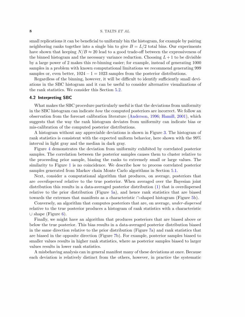
Algorithm 1 SBC generates a histogram from an ensemble of rank statistics of priorsamples relative to corresponding posterior samples. Any deviation from uniformity of thishistogram indicates that the posterior samples are inconsistent with the prior samples. Fora multidimensional problem the procedure is repeated for each parameter or quantity ofinterest to give multiple histograms.

Initialize a histogram with bins centered around 0, . . . , L.

for n in N doDraw a prior sample, θ ∼ π(θ)Draw a simulated data set, y ∼ π(y | θ)Draw posterior samples {θ1, . . . , θL} ∼ π(θ | y)for each one-dimensional random variable, f do

Compute the rank statistic r({f(θ1), . . . , f(θL)}, f(θ)) as defined in (4.1)Increment the histogram with r({f(θ1), . . . , f(θL)}, | f(θ))

Analyze the histogram for uniformity.

relative to the posterior sample,

r({f(θ1), . . . , f(θL)}, f(θ)) =L∑l=1

I[f(θl) < f(θ)] ∈ [0, L],

will be uniformly distributed across the integers [0, L].

Theorem 1. Let θ ∼ π(θ), y ∼ π(y | θ), and {θ1, . . . , θL} ∼ π(θ | y) for any jointdistribution π(y, θ). The rank statistic of any one-dimensional random variable over θ isuniformly distributed over the integers [0, L].

The proof is given in Appendix B.There are many ways of testing the uniformity of the rank statistics, but the SBC

procedure, outlined in Algorithm 1, exploits a histogram of rank statistics for a givenrandom variable to enable visual inspection of uniformity (Figure 3). We first sample Ndraws from the Bayesian joint distribution. For each replicated generated dataset we thensample L exact draws from the posterior distribution and compute the corresponding rankstatistic. We then bin the L rank statistics in a histogram spanning the L + 1 possiblevalues, {0, . . . , L}. If only correlated posteriors samples can be drawn then the procedurecan be modified as discussed in Section 5.1.

In order to help identify deviations, each histogram is complemented with a gray bandindicating 99% of the variation expected from a uniform histogram. Formally, the ver-tical extent of the band extends from the 0.005 quantile to the 0.995 quantile of theBinomial(N, (L+ 1)−1) distribution so that under uniformity we expect that, on average,the counts in only one bin a hundred will deviate outside this band.

In complex problems computational resources often limit the number of replications, N ,and hence the sensitivity of the resulting SBC histogram. In order to reduce the noise from

8 S. TALTS ET AL.

small replications it can be beneficial to uniformly bin the histogram, for example by pairingneighboring ranks together into a single bin to give B = L/2 total bins. Our experimentshave shown that keeping N/B ≈ 20 lead to a good trade-off between the expressiveness ofthe binned histogram and the necessary variance reduction. Choosing L+ 1 to be divisibleby a large power of 2 makes this re-binning easier; for example, instead of generating 1000samples in a problem with known computational limitations we recommend generating 999samples or, even better, 1024− 1 = 1023 samples from the posterior distributions.

Regardless of the binning, however, it will be difficult to identify sufficiently small devi-ations in the SBC histogram and it can be useful to consider alternative visualizations ofthe rank statistics. We consider this Section 5.2.

4.2 Interpreting SBC

What makes the SBC procedure particularly useful is that the deviations from uniformityin the SBC histogram can indicate how the computed posteriors are incorrect. We follow anobservation from the forecast calibration literature (Anderson, 1996; Hamill, 2001), whichsuggests that the way the rank histogram deviates from uniformity can indicate bias ormis-calibration of the computed posterior distributions.

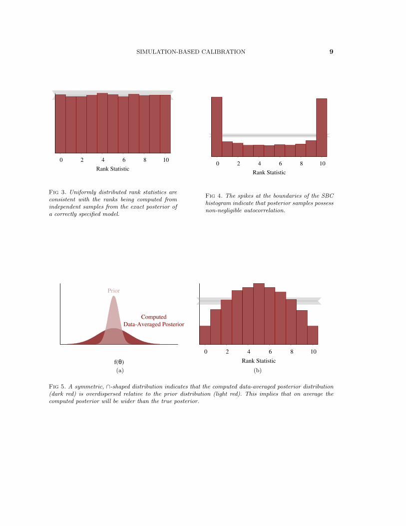
A histogram without any appreciable deviations is shown in Figure 3. The histogram ofrank statistics is consistent with the expected uniform behavior, here shown with the 99%interval in light gray and the median in dark gray.

Figure 4 demonstrates the deviation from uniformity exhibited by correlated posteriorsamples. The correlation between the posterior samples causes them to cluster relative tothe proceeding prior sample, biasing the ranks to extremely small or large values. Thesimilarity to Figure 1 is no coincidence. We describe how to process correlated posteriorsamples generated from Markov chain Monte Carlo algorithms in Section 5.1.

Next, consider a computational algorithm that produces, on average, posteriors thatare overdispersed relative to the true posterior. When averaged over the Bayesian jointdistribution this results in a data-averaged posterior distribution (1) that is overdispersedrelative to the prior distribution (Figure 5a), and hence rank statistics that are biasedtowards the extremes that manifests as a characteristic ∩-shaped histogram (Figure 5b).

Conversely, an algorithm that computes posteriors that are, on average, under-dispersedrelative to the true posterior produces a histogram of rank statistics with a characteristic∪ shape (Figure 6).

Finally, we might have an algorithm that produces posteriors that are biased above orbelow the true posterior. This bias results in a data-averaged posterior distribution biasedin the same direction relative to the prior distribution (Figure 7a) and rank statistics thatare biased in the opposite direction (Figure 7b). For example, posterior samples biased tosmaller values results in higher rank statistics, where as posterior samples biased to largervalues results in lower rank statistics.

A misbehaving analysis can in general manifest many of these deviations at once. Becauseeach deviation is relatively distinct from the others, however, in practice the systematic


0 2 4 6 8 10

Rank Statistic

Fig 3. Uniformly distributed rank statistics areconsistent with the ranks being computed fromindependent samples from the exact posterior ofa correctly specified model.

0 2 4 6 8 10

Rank Statistic

Fig 4. The spikes at the boundaries of the SBChistogram indicate that posterior samples possessnon-negligible autocorrelation.

Prior

ComputedData-Averaged Posterior

f(θ)

(a)

0 2 4 6 8 10

Rank Statistic

(b)

Fig 5. A symmetric, ∩-shaped distribution indicates that the computed data-averaged posterior distribution(dark red) is overdispersed relative to the prior distribution (light red). This implies that on average thecomputed posterior will be wider than the true posterior.

10 S. TALTS ET AL.

Prior

ComputedData-Averaged Posterior

f(θ)

(a)

0 2 4 6 8 10

Rank Statistic

(b)

Fig 6. A symmetric ∪ shape indicates that the computed data-averaged posterior distribution (dark red)is under-dispersed relative to the prior distribution (light red). This implies that on average the computedposterior will be narrower than the true posterior.

PriorComputed

Data-Averaged Posterior

f(θ)

(a)

0 2 4 6 8 10

Rank Statistic

(b)

Fig 7. Asymmetry in the rank histogram indicates that the computed data-averaged posterior distribution(dark red) will be biased in the opposite direction relative to the prior distribution (light red). This impliesthat on average the computed posterior will be biased in the same opposite direction.


deviations are readily separated into the different behaviors if they are large enough.

4.3 Simulation-Based Calibration Plays a Vital Role in a Robust Bayesian Workflow

SBC is one of the few tools for evaluating the critical but frequently unexamined choiceof computational method made in any Bayesian analysis. We have already argued thatperformance on a single simulated observation is, at best, a blunt instrument. Moreover,while most theoretical results only provide asymptotic comfort, SBC adapts to the specificmodel design under consideration.

Furthermore, because SBC validates accuracy through one-dimensional random variableswe can use carefully chosen random variables to make targeted assessments of an analysisbased on our inferential needs and priorities. As these needs and priorities change we canrun SBC again to verify the analysis anew.

The downside of using SBC in practice is that it is expensive; instead of fitting a singleobservation we have to fit N simulated observations before even considering the measureddata. These fits, however, are embarrassingly parallel, which makes it possible to lever-age access to computational resources through multicore personal computers, computingclusters, and cloud computing. For example, all of the examples in Section 6 were run onclusters and took, at most, a few hours.

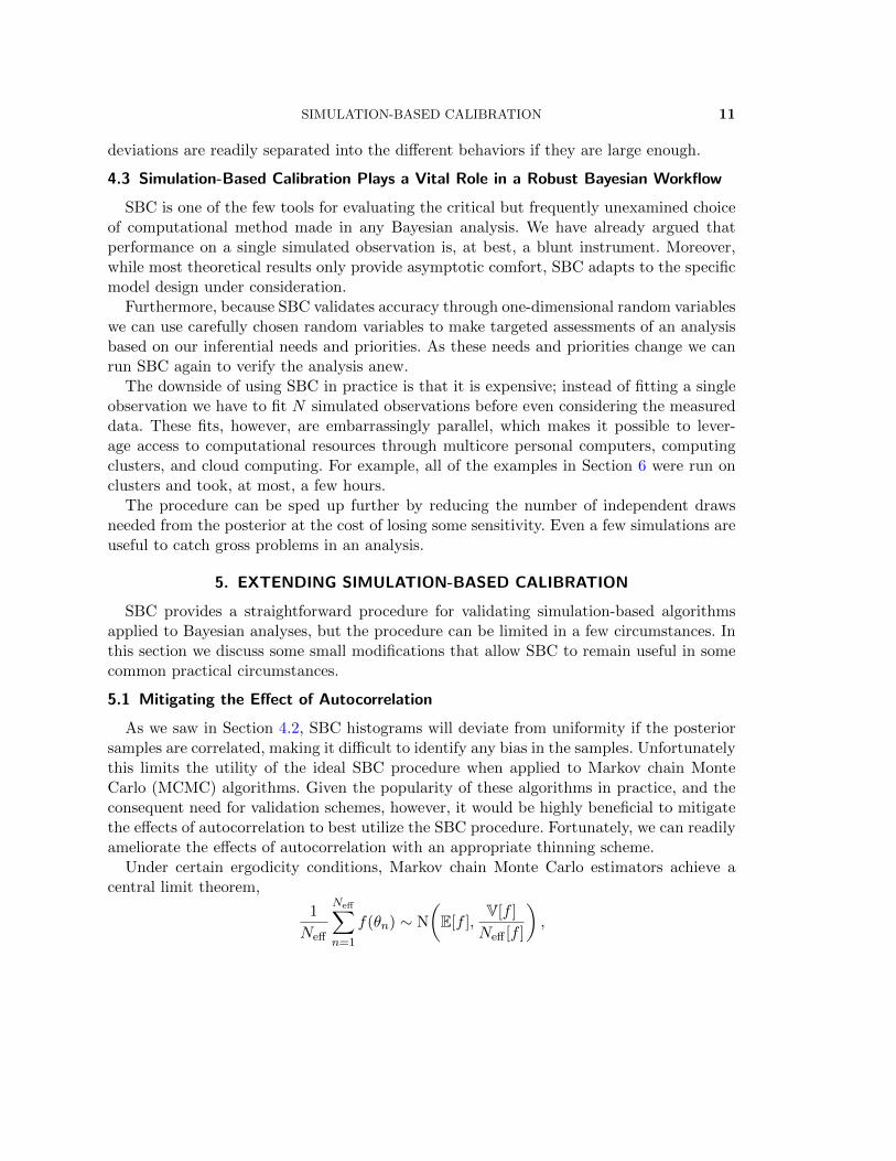
The procedure can be sped up further by reducing the number of independent drawsneeded from the posterior at the cost of losing some sensitivity. Even a few simulations areuseful to catch gross problems in an analysis.

5. EXTENDING SIMULATION-BASED CALIBRATION

SBC provides a straightforward procedure for validating simulation-based algorithmsapplied to Bayesian analyses, but the procedure can be limited in a few circumstances. Inthis section we discuss some small modifications that allow SBC to remain useful in somecommon practical circumstances.

5.1 Mitigating the Effect of Autocorrelation

As we saw in Section 4.2, SBC histograms will deviate from uniformity if the posteriorsamples are correlated, making it difficult to identify any bias in the samples. Unfortunatelythis limits the utility of the ideal SBC procedure when applied to Markov chain MonteCarlo (MCMC) algorithms. Given the popularity of these algorithms in practice, and theconsequent need for validation schemes, however, it would be highly beneficial to mitigatethe effects of autocorrelation to best utilize the SBC procedure. Fortunately, we can readilyameliorate the effects of autocorrelation with an appropriate thinning scheme.

Under certain ergodicity conditions, Markov chain Monte Carlo estimators achieve acentral limit theorem,

1

Neff

Neff∑n=1

f(θn) ∼ N

(E[f ],

V[f ]

Neff [f ]

),

12 S. TALTS ET AL.

where E[f ] is the posterior expectation of a function f , V[f ] is the variance of f , and Neff [f ]is the effective sample size for f ,

Neff [f ] =Nsamp

1 + 2∑∞

m=0 ρm[f ],

with ρm[f ] the lag-m autocorrelation of f , which we estimate from the realized Markovchain (Gelman et al., 2014, Ch. 11). In words, Nsamp correlated samples contains roughlythe same information as Neff exact samples when estimating the expectation of f .

This suggests that thinning a Markov chain by keeping only every Nsamp/Neff [f ] statesshould yield a sample with negligible autocorrelation that is well-suited for the SBC proce-dure with f , giving us (Algorithm 2). By carefully thinning the autocorrelated samples weshould be able to significantly reduce the ∪ shape demonstrated in Figure 4 and maximizethe sensitivity to any remaining issues with the model or algorithm. When running theSBC procedure over multiple quantities of interest we suggest thinning the chain using theminimum Neff [f ].

Algorithm 2 Simulation-based calibration can be applied to the correlated posterior sam-ples generated by a Markov chain provided that the Markov chain can be thinned to Leffective samples at each iteration.

Initialize a histogram with bins centered around 0, . . . , L.

for n in N dodraw a prior sample θ ∼ π(θ)draw a simulated data set y ∼ π(y | θ)run a Markov chain for L′ iterations to generate the correlated posterior samples,{θ1, . . . , θL′} ∼ π(θ | y)

compute the effective sample size, Neff [f ] of {θ1, . . . , θL′} for the function fif Neff [f ] < L then

rerun the Markov for L′ · L/Neff [f ] iterations

uniformly thin the correlated sample to L states and truncate any leftover draws at Lcompute the rank statistic r({f(θ1), . . . , f(θL)}, f(θ)) as defined in (4.1)increment the histogram with r({f(θ1), . . . , f(θL)}, f(θ))

Analyze the histogram for uniformity.

Although some autocorrelation will remain in a sample that has been thinned by ef-fective sample size, our experience has been that this strategy is sufficient to remove theautocorrelation artifacts from the SBC histogram. If desired, more conservative thinningstrategies, such as the truncation rules of Geyer (1992) can remove autocorrelation com-pletely from the sample. A sample thinned with these rules is typically much smaller thanthe sample achieved by thinning based on the effective sample size, and we have not seenany significant benefit for SBC from the increased computation time needed for these moreelaborate thinning methods to date.

Deviations that cannot be mitigated by thinning provide strong evidence that the Markovchain Monte Carlo estimators do not follow a central limit theorem and the Markov chains


are not adequately exploring the target parameter space. This is particularly useful giventhat establishing central limit theorems for particular Markov chains and particular targetdistributions is a notoriously challenging problem even in relatively simple circumstances.

5.2 Simulation-Based Calibration for Small Deviations

The SBC histogram provides a general and interpretable means of identifying deviationsfrom uniformity of the rank statistics and hence inaccuracies in our posterior computa-tion, at least when the inaccuracies are large enough. For small deviations, however, theSBC histogram may not be sensitive enough for the deviations to be evident and othervisualization strategies may be advantageous.

One option is to bin the SBC histogram multiple times to see if any deviation persistsregardless of the binning. This approach, however, is ungainly to implement when thereare many parameters and can be difficult to interpret. In particular, considering multiplehistograms introduces a vulnerability to multiple testing biases.

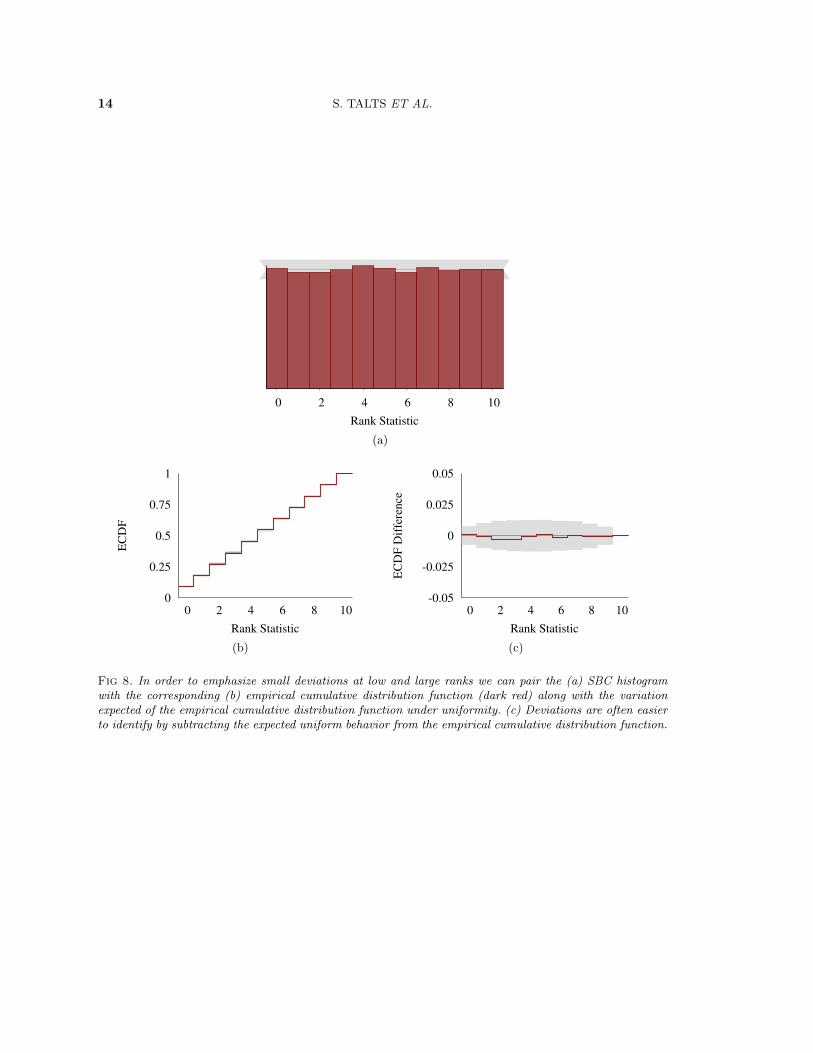
Another approach is to pair the SBC histogram with the empirical cumulative distribu-tion function (ECDF) which reduces variation at small and large ranks, making it easier toidentify deviations around those values (Figure 8b). The deviation of the empirical CDFaway from the expected uniform behavior is especially useful for identifying these smalldeviations (Figure 8c).

More subtle deviations can be isolated by considering more particular summary statistics,such as ranks quantiles or averages. While these have the potential to identify small biasesthey can also be harder to interpret and not as sensitive to the systematic deviations thatmanifest in the SBC histogram. Identifying a robust suite of diagnostic statistics is an openarea of research and at present we recommend using the SBC histogram whenever possible.

6. EXPERIMENTS

In this section we consider the application of SBC on a series of examples that demon-strates the utility of the procedure for identifying and correcting incorrectly implementedanalyses. For each example we implement the SBC procedure using posterior samplesL = 100 so that, if the algorithm is properly calibrated, then the rank statistics will followa U [0, 100] discrete uniform distribution. The experiments in Section 6.1 through Section6.3 used N = 10, 000 replicated observations while the experiment in Section 6.4 usedN = 1000 replicated observations.

6.1 Misspecified Prior

Let’s first consider the case where we build our posterior using a different prior thanthat which we use to generate prior samples. This is not an uncommon mistake, even whenmodels are specified in probabilistic programming languages.

Consider the linear regression model that we used before (Listing 2 in the Appendix)but with the prior on β modified to N(0, 12). With the prior samples still drawn accordingto N(0, 102), we expect that the posterior for β will be under-dispersed relative to the prior

14 S. TALTS ET AL.

0 2 4 6 8 10

Rank Statistic

(a)

0

0.25

0.5

0.75

1

0 2 4 6 8 10

EC

DF

Rank Statistic

(b)

-0.05

-0.025

0

0.025

0.05

0 2 4 6 8 10

EC

DF

Dif

fere

nce

Rank Statistic

(c)

Fig 8. In order to emphasize small deviations at low and large ranks we can pair the (a) SBC histogramwith the corresponding (b) empirical cumulative distribution function (dark red) along with the variationexpected of the empirical cumulative distribution function under uniformity. (c) Deviations are often easierto identify by subtracting the expected uniform behavior from the empirical cumulative distribution function.


0 20 40 60 80 100

Rank Statistic

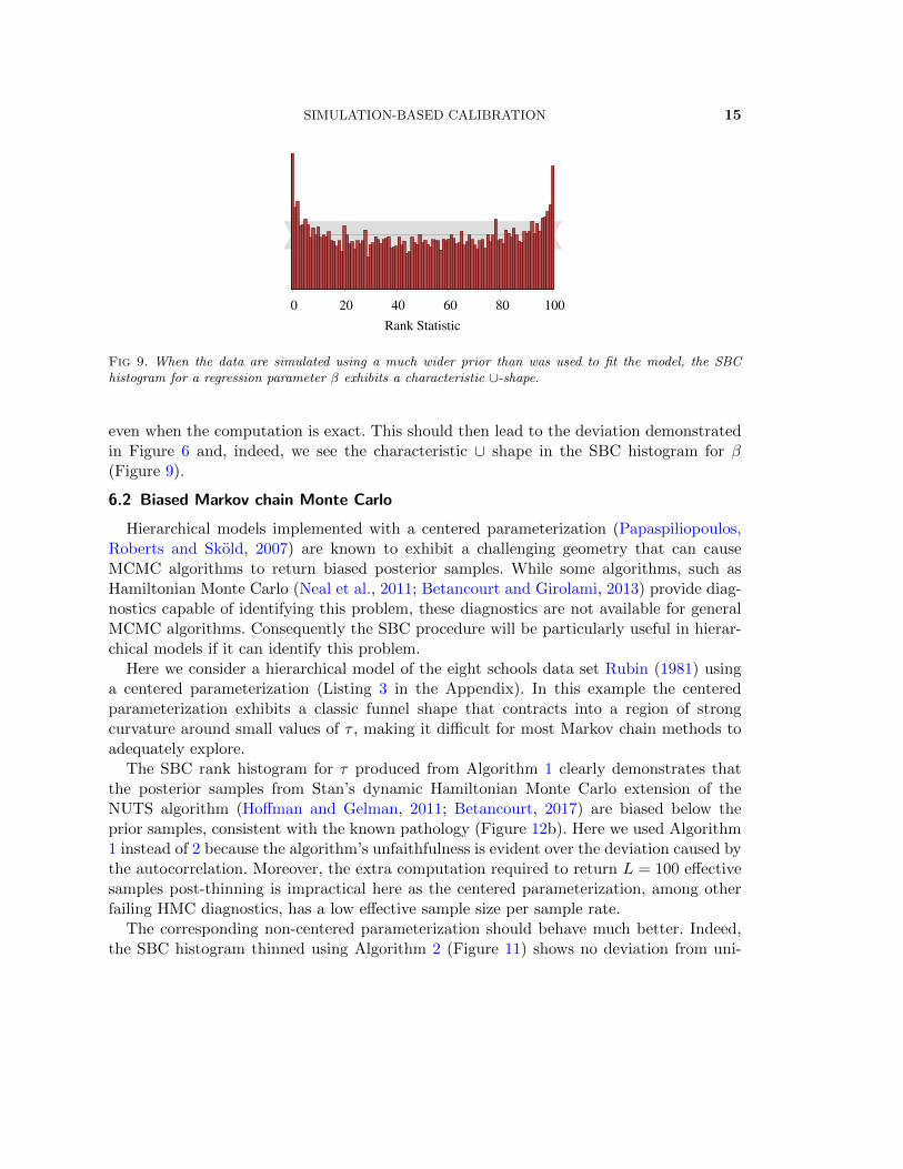
Fig 9. When the data are simulated using a much wider prior than was used to fit the model, the SBChistogram for a regression parameter β exhibits a characteristic ∪-shape.

even when the computation is exact. This should then lead to the deviation demonstratedin Figure 6 and, indeed, we see the characteristic ∪ shape in the SBC histogram for β(Figure 9).

6.2 Biased Markov chain Monte Carlo

Hierarchical models implemented with a centered parameterization (Papaspiliopoulos,Roberts and Skold, 2007) are known to exhibit a challenging geometry that can causeMCMC algorithms to return biased posterior samples. While some algorithms, such asHamiltonian Monte Carlo (Neal et al., 2011; Betancourt and Girolami, 2013) provide diag-nostics capable of identifying this problem, these diagnostics are not available for generalMCMC algorithms. Consequently the SBC procedure will be particularly useful in hierar-chical models if it can identify this problem.

Here we consider a hierarchical model of the eight schools data set Rubin (1981) usinga centered parameterization (Listing 3 in the Appendix). In this example the centeredparameterization exhibits a classic funnel shape that contracts into a region of strongcurvature around small values of τ , making it difficult for most Markov chain methods toadequately explore.

The SBC rank histogram for τ produced from Algorithm 1 clearly demonstrates thatthe posterior samples from Stan’s dynamic Hamiltonian Monte Carlo extension of theNUTS algorithm (Hoffman and Gelman, 2011; Betancourt, 2017) are biased below theprior samples, consistent with the known pathology (Figure 12b). Here we used Algorithm1 instead of 2 because the algorithm’s unfaithfulness is evident over the deviation caused bythe autocorrelation. Moreover, the extra computation required to return L = 100 effectivesamples post-thinning is impractical here as the centered parameterization, among otherfailing HMC diagnostics, has a low effective sample size per sample rate.

The corresponding non-centered parameterization should behave much better. Indeed,the SBC histogram thinned using Algorithm 2 (Figure 11) shows no deviation from uni-

16 S. TALTS ET AL.

0 20 40 60 80 100

Rank Statistic

(a)

0 20 40 60 80 100

Rank Statistic

(b)

Fig 10. Even without thinning, the underlying Markov chains, the SBC histograms for θ[1] and τ in the 8schools centered parameterization of Section 6.2 demonstrate that Hamiltonian Monte Carlo yields samplesthat are biased towards larger values of τ than were used to generate the data.

0 20 40 60 80 100

Rank Statistic

(a)

0 20 40 60 80 100

Rank Statistic

(b)

Fig 11. Once thinned, the SBC histogram for θ[1] and τ from the 8 schools non-centered parameterizationin Section 6.2 show no evidence of bias.


0 20 40 60 80 100

Rank Statistic

(a)

0 20 40 60 80 100

Rank Statistic

(b)

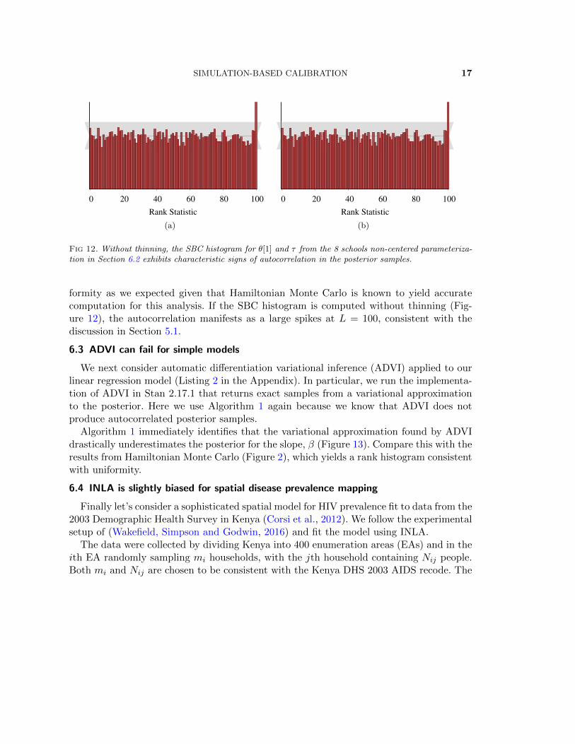
Fig 12. Without thinning, the SBC histogram for θ[1] and τ from the 8 schools non-centered parameteriza-tion in Section 6.2 exhibits characteristic signs of autocorrelation in the posterior samples.

formity as we expected given that Hamiltonian Monte Carlo is known to yield accuratecomputation for this analysis. If the SBC histogram is computed without thinning (Fig-ure 12), the autocorrelation manifests as a large spikes at L = 100, consistent with thediscussion in Section 5.1.

6.3 ADVI can fail for simple models

We next consider automatic differentiation variational inference (ADVI) applied to ourlinear regression model (Listing 2 in the Appendix). In particular, we run the implementa-tion of ADVI in Stan 2.17.1 that returns exact samples from a variational approximationto the posterior. Here we use Algorithm 1 again because we know that ADVI does notproduce autocorrelated posterior samples.

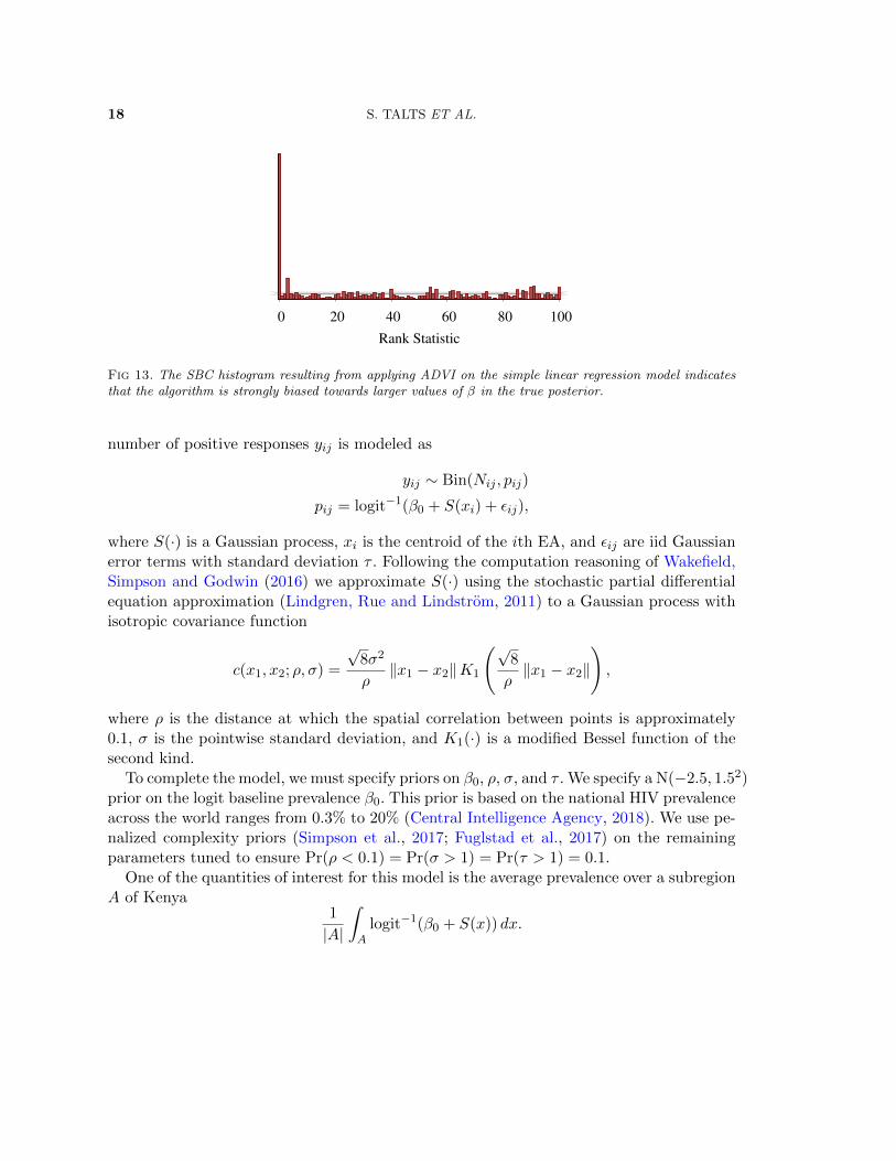
Algorithm 1 immediately identifies that the variational approximation found by ADVIdrastically underestimates the posterior for the slope, β (Figure 13). Compare this with theresults from Hamiltonian Monte Carlo (Figure 2), which yields a rank histogram consistentwith uniformity.

6.4 INLA is slightly biased for spatial disease prevalence mapping

Finally let’s consider a sophisticated spatial model for HIV prevalence fit to data from the2003 Demographic Health Survey in Kenya (Corsi et al., 2012). We follow the experimentalsetup of (Wakefield, Simpson and Godwin, 2016) and fit the model using INLA.

The data were collected by dividing Kenya into 400 enumeration areas (EAs) and in theith EA randomly sampling mi households, with the jth household containing Nij people.Both mi and Nij are chosen to be consistent with the Kenya DHS 2003 AIDS recode. The

18 S. TALTS ET AL.

0 20 40 60 80 100

Rank Statistic

Fig 13. The SBC histogram resulting from applying ADVI on the simple linear regression model indicatesthat the algorithm is strongly biased towards larger values of β in the true posterior.

number of positive responses yij is modeled as

yij ∼ Bin(Nij , pij)

pij = logit−1(β0 + S(xi) + εij),

where S(·) is a Gaussian process, xi is the centroid of the ith EA, and εij are iid Gaussianerror terms with standard deviation τ . Following the computation reasoning of Wakefield,Simpson and Godwin (2016) we approximate S(·) using the stochastic partial differentialequation approximation (Lindgren, Rue and Lindstrom, 2011) to a Gaussian process withisotropic covariance function

c(x1, x2; ρ, σ) =

√8σ2

ρ‖x1 − x2‖K1

(√8

ρ‖x1 − x2‖

),

where ρ is the distance at which the spatial correlation between points is approximately0.1, σ is the pointwise standard deviation, and K1(·) is a modified Bessel function of thesecond kind.

To complete the model, we must specify priors on β0, ρ, σ, and τ . We specify a N(−2.5, 1.52)prior on the logit baseline prevalence β0. This prior is based on the national HIV prevalenceacross the world ranges from 0.3% to 20% (Central Intelligence Agency, 2018). We use pe-nalized complexity priors (Simpson et al., 2017; Fuglstad et al., 2017) on the remainingparameters tuned to ensure Pr(ρ < 0.1) = Pr(σ > 1) = Pr(τ > 1) = 0.1.

One of the quantities of interest for this model is the average prevalence over a subregionA of Kenya

1

|A|

∫A

logit−1(β0 + S(x)) dx.


0 20 40 60 80 100

Rank Statistic

(a)

0

0.25

0.5

0.75

1

0 20 40 60 80 100

EC

DF

Rank Statistic

(b)

-0.05

-0.025

0

0.025

0.05

0 20 40 60 80 100

EC

DF

Dif

fere

nce

Rank Statistic

(c)

Fig 14. (a) The SBC histogram for the average prevalence of a spatial model doesn’t exhibit any obviousdeviations, although the large span of the expected variation (gray) suggests that the SBC histogram may beunderpowered. (b) The empirical cumulative distribution function (dark red), however, shows that there isa small deviation at low ranks beyond the variation expected from a uniform distribution (gray). (c) Thedeviation is more evident by looking at the difference between the empirical cumulative distribution functionand the stepwise-linear behavior expected of a discrete uniform distribution.

Wakefield, Simpson and Godwin (2016) suggested fitting this model using the R-INLA pack-age to speed up the computation. As the quantity of interest is a non-linear transformationof a number of parameters, we need to use the R-INLA’s approximate posterior sampler,which is a relatively recent feature (Seppa et al., 2017).

Figure 14a shows the SBC histogram for N = 1000 replications to which are limitedgiven the relatively high cost to run INLA in this model. The histogram shows that all ofthe ranks fall within the gray bars, but the large span of the bars indicates that the visualdiagnostic may be underpowered. In our tests, we saw that it’s common for deviationsfrom a uniform distribution to be sufficiently severe that this histogram will still exhibitthe signs of a poorly fitting procedure. Hence for a more fine-scale view of the fit we followthe recommendation in Section 5.2 and consider the ECDF (Figure 14b, c). Here we see

20 S. TALTS ET AL.

that low ranks are seen slightly more often in the computed ranks than we would expectfrom a uniform distribution.

It is not surprising that INLA exhibits some bias in this example. Binomial data withlow expected counts does not contain much information, which poses some problems for theLaplace approximation. Even though this feature is only present when the observed valuesof yij/Nij are close to zero, the SBC procedure is a sufficiently sensitive instrument toidentify the problem. Overall, we would view INLA as a good approximation in a countrylike Kenya where the national prevalence is around 5.4%, while it would be inappropriate inAustralia where the prevalence is 0.1% (Central Intelligence Agency, 2018). If we repeatedthis type of survey in a country with only 0.1% prevalence, however, then we would endup with too many zero observations for the method to be useful.

7. CONCLUSION

In this paper, we introduce SBC, a readily-implemented procedure that can identifysources of poorly implemented analyses, including biased computational algorithms or in-correct model specifications. The visualizations produced by the procedure allow us to notonly identify that a problem exists but also learn how the problem will affect resultinginferences. The ability to both identify and interpret these issues makes SBC an importantstep in a robust Bayesian workflow.

Our reliance on interpreting the SBC diagnostic through visualization, however, can bea limitation in practice, especially when dealing with models featuring a large numberof parameters. One immediate direction for future work is to develop reliable numericalsummaries that quantify deviations from uniformity of each SBC histogram and provideautomated diagnostics that can flag certain parameters for closer inspection.

Global summaries, such as a χ2 goodness-of-fit test of the SBC histogram with respectto a uniform response, are natural options, but we have found that they do not performparticularly well for this problem. The reason for this is that the deviation from uniformitytends to occur in only a few systematic ways, as discussed in Section 4.2, whereas thesetests consider only global behavior and hence do not exploit these known failure modes. Apotential alternative is to report a number of summaries that are designed to be sensitiveto the specific types of deviation from uniformity we might expect to see.

Another future direction is deriving the expected behavior of the SBC histograms in thepresence of autocorrelation and dropping the thinning requirement of SBC. This could evenbe done empirically, using the output of chains with known autocorrelations to calibratethe deviations in the rank histograms. These calibrated deviations could be used to definea sense of effective sample size for any algorithm capable of generating samples, not justMarkov chain Monte Carlo.

Finally, the SBC histograms are only able to assess the calibration of one-dimensionalposterior summaries. This is a limitation, especially in situations where the quantities ofinterest are naturally multivariate. An interesting extension of this methodology would be


to incorporate some of the advances in multivariate calibration of probabilistic forecasts(Gneiting et al., 2008; Thorarinsdottir, Scheuerer and Heinz, 2013).

Acknowledgements. We thank Bob Carpenter, Chris Ferro, and Mitzi Morris for theirhelpful comments. The plot in Figure 14(c) shares the same derivation as the inla.ks.plot()function written by Finn Lindgren and found in the R-INLA package. We thank Academyof Finland (grant 313122), Sloan Foundation (grant G-2015-13987), U.S. National Sci-ence Foundation (grant CNS-1730414), Office of Naval Research (grants N00014-15-1-2541and N00014-16-P-2039), and Defense Advanced Research Projects Agency (grant DARPABAA-16-32) for partial support of this research.

REFERENCES

Central Intelligence Agency (2018). COUNTRY COMPARISON :: HIV/AIDS - ADULTPREVALENCE RATE. The World Factbook. https://www.cia.gov/library/publications/the-world-factbook/rankorder/2155rank.html. Accessed: 2018-04-04.

Anderson, J. L. (1996). A method for producing and evaluating probabilistic forecasts from ensemblemodel integrations. Journal of Climate 9 1518–1530.

Betancourt, M. (2017). A conceptual introduction to Hamiltonian Monte Carlo. arXiv preprintarXiv:1701.02434.

Betancourt, M. J. and Girolami, M. (2013). Hamiltonian Monte Carlo for Hierarchical Models.Carpenter, B., Gelman, A., Hoffman, M., Lee, D., Goodrich, B., Betancourt, M., Brubaker, M.,

Guo, J., Li, P. and Riddell, A. (2017). Stan: A Probabilistic Programming Language. Journal ofStatistical Software, Articles 76 1–32.

Cook, S. R., Gelman, A. and Rubin, D. B. (2006). Validation of Software for Bayesian Models UsingPosterior Quantiles. J. Comput. Graph. Stat. 15 675–692.

Corsi, D. J., Neuman, M., Finlay, J. E. and Subramanian, S. (2012). Demographic and health surveys:a profile. International journal of epidemiology 41 1602–1613.

Fuglstad, G.-A., Simpson, D., Lindgren, F. and Rue, H. (2017). Constructing priors that penalize thecomplexity of Gaussian random fields. Journal of the American Statistical Association Accepted.

Gelman, A. (2017). Correction to Cook, Gelman, and Rubin (2006). J. Comput. Graph. Stat. 26 940.Gelman, A., Carlin, J. B., Stern, H. S., Dunson, D. B., Vehtari, A. and Rubin, D. B. (2014).

Bayesian Data Analysis, third edition. CRC Press.Geweke, J. (2004). Getting it right: Joint distribution tests of posterior simulators. J. Am. Stat. Assoc.Geyer, C. J. (1992). Practical Markov chain Monte Carlo. Statistical science 473–483.Gneiting, T., Stanberry, L. I., Grimit, E. P., Held, L. and Johnson, N. A. (2008). Assessing proba-

bilistic forecasts of multivariate quantities, with an application to ensemble predictions of surface winds.Test 17 211.

Hamill, T. M. (2001). Interpretation of rank histograms for verifying ensemble forecasts. Monthly WeatherReview 129 550–560.

Hoffman, M. D. and Gelman, A. (2011). The No-U-Turn Sampler: Adaptively Setting Path Lengths inHamiltonian Monte Carlo.

Kucukelbir, A., Tran, D., Ranganath, R., Gelman, A. and Blei, D. M. (2017). Automatic differen-tiation variational inference. The Journal of Machine Learning Research 18 430–474.

Lindgren, F., Rue, H. and Lindstrom, J. (2011). An explicit link between Gaussian fields and Gaus-sian Markov random fields: the stochastic partial differential equation approach. Journal of the RoyalStatistical Society: Series B (Statistical Methodology) 73 423–498.

Neal, R. M. et al. (2011). MCMC using Hamiltonian dynamics. Handbook of Markov Chain Monte Carlo2.

22 S. TALTS ET AL.

Papaspiliopoulos, O., Roberts, G. O. and Skold, M. (2007). A general framework for the parametriza-tion of hierarchical models. Statistical Science 59–73.

Rubin, D. B. (1981). Estimation in Parallel Randomized Experiments. Journal of Educational Statistics 6377-401.

Rue, H., Martino, S. and Chopin, N. (2009). Approximate Bayesian inference for latent Gaussian modelsby using integrated nested Laplace approximations. Journal of the royal statistical society: Series b(statistical methodology) 71 319–392.

Rue, H., Riebler, A., Sørbye, S. H., Illian, J. B., Simpson, D. P. and Lindgren, F. K. (2017).Bayesian computing with INLA: a review. Annual Review of Statistics and Its Application 4 395–421.

Seppa, K., Rue, H., Hakulinen, T., Laara, E., Sillanpaa, M. J. and Pitkniemi, J. (2017). Estimat-ing multilevel regional variation in excess mortality of cancer patients using integrated nested Laplaceapproximation. Submitted.

Simpson, D., Rue, H., Riebler, A., Martins, T. G., Sørbye, S. H. et al. (2017). Penalising modelcomponent complexity: A principled, practical approach to constructing priors. Statistical science 321–28.

Thorarinsdottir, T. L., Scheuerer, M. and Heinz, C. (2013). Assessing the calibration of high-dimensional ensemble forecasts using rank histograms. Journal of Computational and Graphical Statistics25 105–122.

Wakefield, J., Simpson, D. and Godwin, J. (2016). Comment: Getting into Space with a Weight Problem.Journal of the American Statistical Association 111 1111–1118.


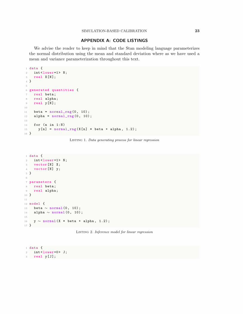
APPENDIX A: CODE LISTINGS

We advise the reader to keep in mind that the Stan modeling language parameterizesthe normal distribution using the mean and standard deviation where as we have used amean and variance parameterization throughout this text.

1 data {

2 int <lower=1> N;

3 real X[N];

4 }

5

6 generated quantities {

7 real beta;

8 real alpha;

9 real y[N];

10

11 beta = normal_rng (0, 10);

12 alpha = normal_rng (0, 10);

13

14 for (n in 1:N)

15 y[n] = normal_rng(X[n] * beta + alpha , 1.2);

16 }

Listing 1. Data generating process for linear regression

1 data {

2 int <lower=1> N;

3 vector[N] X;

4 vector[N] y;

5 }

6

7 parameters {

8 real beta;

9 real alpha;

10 }

11

12 model {

13 beta ∼ normal(0, 10);

14 alpha ∼ normal(0, 10);

15

16 y ∼ normal(X * beta + alpha , 1.2);

17 }

Listing 2. Inference model for linear regression

1 data {

2 int <lower=0> J;

3 real y[J];

24 S. TALTS ET AL.

4 real <lower=0> sigma[J];

5 }

6

7 parameters {

8 real mu;

9 real <lower=0> tau;

10 real theta[J];

11 }

12

13 model {

14 mu ∼ normal(0, 5);

15 tau ∼ normal(0, 5);

16 theta ∼ normal(mu, tau);

17 y ∼ normal(theta , sigma);

18 }

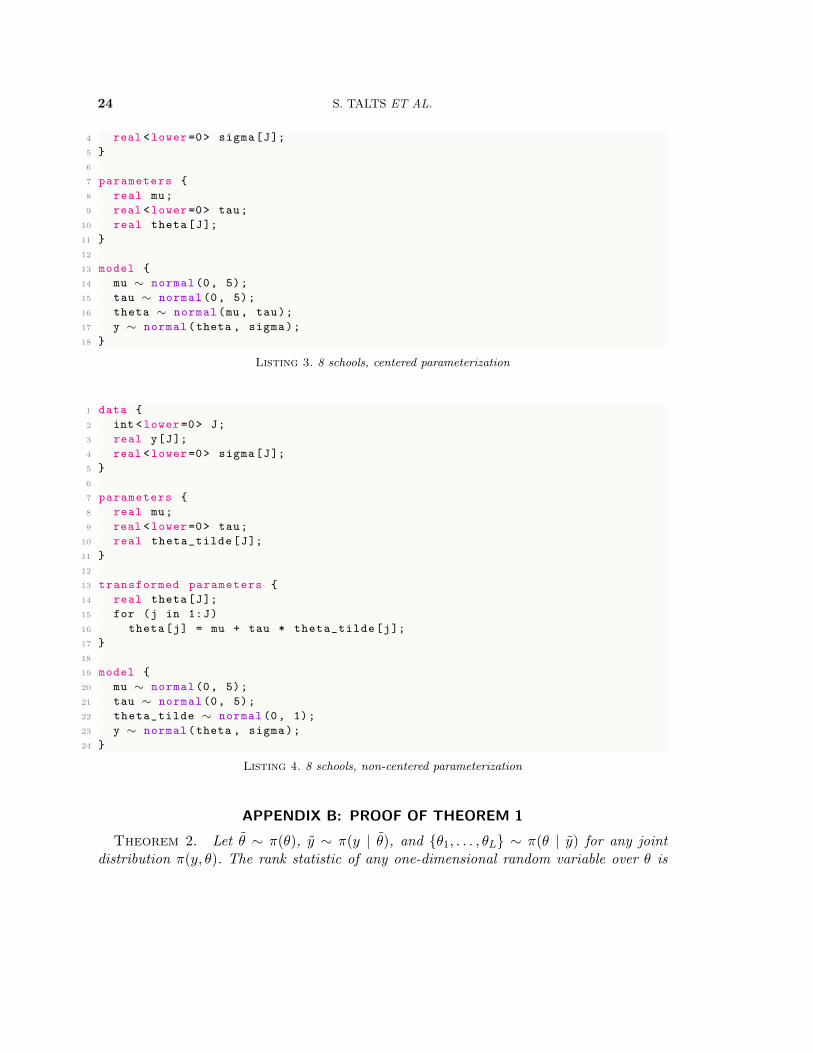
Listing 3. 8 schools, centered parameterization

1 data {

2 int <lower=0> J;

3 real y[J];

4 real <lower=0> sigma[J];

5 }

6

7 parameters {

8 real mu;

9 real <lower=0> tau;

10 real theta_tilde[J];

11 }

12

13 transformed parameters {

14 real theta[J];

15 for (j in 1:J)

16 theta[j] = mu + tau * theta_tilde[j];

17 }

18

19 model {

20 mu ∼ normal(0, 5);

21 tau ∼ normal(0, 5);

22 theta_tilde ∼ normal(0, 1);

23 y ∼ normal(theta , sigma);

24 }

Listing 4. 8 schools, non-centered parameterization

APPENDIX B: PROOF OF THEOREM 1

Theorem 2. Let θ ∼ π(θ), y ∼ π(y | θ), and {θ1, . . . , θL} ∼ π(θ | y) for any jointdistribution π(y, θ). The rank statistic of any one-dimensional random variable over θ is


uniformly distributed over the integers [0, L].

Proof. Consider the one-dimensional random variable f : Θ→ R and let f = f(θ) bethe evaluation of the random variable with respect to the prior sample with fn = f(θn)the evaluation of the random variable with respect to the posterior sample.

Without loss of generality, relabel the elements of the posterior sample such that theyare ordered with respect to the random variable,

f1 ≤ f2 ≤ . . . ≤ fL−1 ≤ fL.

We can then write the probability mass function of the rank statistic r({f1, . . . , fL}, f) as

ρ(r | f) = P[{f1, . . . , fr} < f ≤ {fr+1, . . . , fL}]

=L!

r! (L− r)!

r∏l=1

P[fl < f ]×L∏

l=r+1

P[f ≤ fl],

=L!

r! (L− r)!

r∏l=1

P (f)×L∏

l=r+1

(1− P (f)

),

where the symmetry factor accounts for the possible orderings of the elements below andabove the cutoff f .

Because the posterior samples are identically and independently distributed this imme-diately reduces to a Binomial distribution,

ρ(r | f) =L!

r! (L− r)!

r∏l=1

P (f)×L∏

l=r+1

(1− P (f)

)=

L!

r! (L− r)!

(P (f)

)r×(

1− P (f))L−r

= Binomial(r | L,P (f)).

Marginalizing over the possible values of f then gives

ρ(r) =

∫df π(f) ρ(r | f)

=

∫df π(f) Binomial(k | N,P (f)).

Changing variables to p(f) =∫ f

0 df ′π(f ′) yields

ρ(r) =

∫ 1

0dpBinomial(k | N,P (f(p))),

26 S. TALTS ET AL.

but because the prior sample is identically distributed to the posterior samples we haveP (f(p)) = p and the probability mass function becomes

ρ(r) =

∫ 1

0dpBinomial(r | L, p)

=L!

r! (L− r)!

∫ 1

0dp pr(1− p)L−r

=L!

r! (L− r)!r! (L− r)!(L+ 1)!

=1

L+ 1.

Consequently the rank statistic is uniformly distributed across its L + 1 possible integervalues, [0, . . . , L].

validating bayesian inference algorithms with simulation … procedure can be sped up further by...

Documents