validation of bim components by photogrammetric

VALIDATION OF BIM COMPONENTS BY PHOTOGRAMMETRIC POINT CLOUDSFOR CONSTRUCTION SITE MONITORING

S. Tuttasa, ∗, A. Braunb, A. Borrmannb, U. Stillaa

a Photogrammetry & Remote Sensing, TU Munchen, 80290 Munchen, Germany - (sebastian.tuttas, stilla)@tum.deb Computational Modeling and Simulation, TU Munchen, 80290 Munchen, Germany -

(alex.braun, andre.borrmann)@tum.de

Commission III, WG III/4

KEY WORDS: photogrammetric point cloud, construction site monitoring, 3D building model, BIM

ABSTRACT:

Construction progress monitoring is a primarily manual and time consuming process which is usually based on 2D plans and thereforehas a need for an increased automation. In this paper an approach is introduced for comparing a planned state of a building (as-planned)derived from a Building Information Model (BIM) to a photogrammetric point cloud (as-built). In order to accomplish the comparisona triangle-based representation of the building model is used. The approach has two main processing steps. First, visibility checks areperformed to determine whether or not elements of the building are potentially built. The remaining parts can be either categorized asfree areas, which are definitely not built, or as unknown areas, which are not visible. In the second step it is determined if the potentiallybuilt parts can be confirmed by the surrounding points. This process begins by splitting each triangle into small raster cells. For eachraster cell a measure is calculated using three criteria: the mean distance of the points, their standard deviation and the deviation froma local plane fit. A triangle is confirmed if a sufficient number of raster cells yield a high rating by the measure. The approach istested based on a real case inner city scenario. Only triangles showing unambiguous results are labeled with their statuses, because it isintended to use these results to infer additional statements based on dependencies modeled in the BIM. It is shown that the label builtis reliable and can be used for further analysis. As a drawback this comes with a high percentage of ambiguously classified elements,for which the acquired data is not sufficient (in terms of coverage and/or accuracy) for validation.

1. INTRODUCTION

1.1 Motivation

A Building Information Model (BIM) contains the 3D geometryof a building, as well as the process information of the construc-tion what makes the 3D to a 4D building model. For progressmonitoring, the planned states (as-planned) of the constructionhave to be validated against the actual state (as-built) at a cer-tain time step. Today this is a primarily manual process whichis usually based on 2D plans. Because of the dynamic processsequences of construction projects, it has to be assumed that theactual execution of the construction work differs strongly fromthe planning at the beginning of the project. Reasons for this gapare, among others, delivery delays, delays in construction and thestrong dependencies between the single processes. For detect-ing deviations from the schedule as quickly as possible, allow-ing a prompt response, an automatic construction progress mon-itoring system is desirable, which works directly with the BIM.The detected deviations lead to modifications of the schedule andthe following processes modeled in the BIM. Difficulties on con-struction sites for the monitoring arise because of occlusions, theoccurrence of various temporal objects or the limited accessibilityof acquisition positions. The goal is to derive a statement aboutthe status of a certain building element at a certain time step basedon the obtainable data. Therefore a measure which can cope withocclusions and noisy sections of the point cloud is needed.

1.2 Related Work

The basic acquisition techniques for construction site monitoringare laser scanning and image-based/photogrammetric methods.

∗Corresponding author

The following approaches are based on one or both of theses tech-niques. In (Bosche and Haas, 2008) and (Bosche, 2010) a systemfor as-built as-planned comparison based on laser scanning data isintroduced. The co-registration of point cloud and model is per-formed by an adapted Iterative-Closest-Point-Algorithm (ICP).Within this system, the as-planned model is converted to a simu-lated point cloud by using the known positions of the laser scan-ner. The percentage of simulated points which are verified by thelaser scan is used as verification measure. (Turkan et al., 2012),(Turkan et al., 2013) and (Turkan et al., 2014) use and extend thissystem for progress tracking using schedule information, for es-timating the progress in terms of earned value, and for detectionof secondary objects. (Kim et al., 2013b) detect specific com-ponent types using a supervised classification based on Lalondefeatures derived from the as-built point cloud. If the object typeobtained from the classification coincides with the type in themodel, the object is regarded as verified. As in the method above,the model has to be sampled into a point representation. A differ-ent method to decide if a building element is present is introducedby (Zhang and Arditi, 2013). Four different cases can be distin-guished (point cloud represents a completed object, a partiallycompleted object, a different object or the object is not in place)by analyzing the relationship of points within the boundaries ofthe object to the boundaries of a shrunk object. The authors testtheir approach in a simplified test environment, which does notinclude any problems occurring on a real construction site.The usage of cameras as acquisition device comes with the dis-advantage of a lower geometric accuracy compared to the laserscanning point clouds. However, cameras have the advantagethat they can be used in a more flexible manner and their costsare lower. Therefore, other processing strategies are need if im-age data instead of laser scanning is used. An overview andcomparison of image-based approaches for construction progress

ISPRS Annals of the Photogrammetry, Remote Sensing and Spatial Information Sciences, Volume II-3/W4, 2015 PIA15+HRIGI15 – Joint ISPRS conference 2015, 25–27 March 2015, Munich, Germany

This contribution has been peer-reviewed. The double-blind peer-review was conducted on the basis of the full paper. doi:10.5194/isprsannals-II-3-W4-231-2015

231

monitoring is given by (Rankohi and Waugh, 2014). (Ibrahimet al., 2009) introduce an approach with a single, fixed camera.They analyze the changes of consecutive images acquired every15 minutes. The building elements are projected to the image andstrong changes within these regions are used as detection criteria.This approach suffers from the fact that often changes occur dueto different reasons than the completion of a building element.(Kim et al., 2013a) also use a fixed camera and image processingtechniques for the detection of new construction elements. Theresults are used to update the construction schedule. Since manyfixed cameras would be necessary to cover a whole constructionsite, more approaches, like the following and the one presentedin this paper, rely on images from hand-held cameras to cover thecomplete construction site.In contrast to a point cloud received from a laser scan a scale hasto be introduced to a photogrammetric point cloud. A possibilityis to use a stereo-camera system, as done in (Son and Kim, 2010),(Brilakis et al., 2011) or (Fathi and Brilakis, 2011). (Rashidiet al., 2014) propose to use a colored cube with known size astarget, which can be automatically measured to determine thescale. In (Golparvar-Fard et al., 2011a) image-based approachesare compared with laser-scanning results. The artificial test datais strongly simplified and the real data experiments are limitedto a very small part of a construction site. In this case no scalewas introduced to the photogrammetric measurements leading toaccuracy measures which are only relative. (Golparvar-Fard etal., 2011b) and (Golparvar-Fard et al., 2012) use unstructuredimages of a construction site to create a point cloud. The im-ages are oriented using a Structure-from-Motion process (SfM).Subsequently, dense point clouds are calculated. For the as-builtas-planned comparison, the scene is discretized into a voxel grid.The construction progress is determined by a probabilistic ap-proach. The thresholds for the detection parameters are calcu-lated by supervised learning. In this framework, occlusions aretaken into account. The approach relies on the discretization ofthe space by the voxel grid with a cube size of a few centimeters.Although, a grid is also used in our approach, the deviation ofthe point cloud to the building model is calculated exactly andused within a weighting function for the validation of buildingelements. In contrast to most of the discussed publications, wepresent a test site which presents extra challenges for progressmonitoring due to the existence of a large number of disturbingobjects, such as scaffolding.

1.3 Contribution and structure of the paper

In this paper we explain the method described in (Tuttas et al.,2014a) in more detail and add a more comprehensive evaluationof the results. In previous publications only a very small test areacould be used for evaluation. Now, the model of the completebuilding is used. Additionally the effects using a triangle meshand not rectangular shaped objects are investigated and discussed.With the triangle mesh also curved parts are considered, leadingto very small triangles at some parts of the building. The imageorientation process, the generation of the dense 3D point cloudand the co-registration are described in (Tuttas et al., 2014a),(Tuttas et al., 2014b) and (Braun et al., 2014). The method for theas-built as-planned comparison is described in Chapter 2. It con-sists of one part using visibility constraints (Section 2.2) and an-other part using points extracted in the surrounding of the modelplanes (Section 2.3). Results for two time steps of a construc-tion site are shown in Chapter 3, followed by a discussion and anoutlook in Chapter 4.

2. METHODS

2.1 Overview of the as-built as-planned comparison process

For the as-built as-planned comparison process, two different kindof grids are used. For checking visibility constraints, meaning tocheck which building elements are visible based on the rays fromthe cameras to the reconstructed points, a voxel grid with cells ofsize o is created. This grid is generated for the whole construc-tion site area. Additionally every triangle-plane of the as-plannedmodel is split into quadratic raster cells of size r. Both gridsare depicted in Figure 1 together with a building element’s sur-face which is split into two triangles. The voxel grid is shownin orange, the raster cells are shown in green. The voxel grid istypically not aligned orthogonally to the model planes (as it is forsimplicity here in the figure), but to the coordinate system axes ofthe model. The center point shown in the figure is used as a ref-erence coordinate for the raster cells. The bounding box aroundeach raster cell is used to extract points in front and behind themodel plane with the maximum distance b.

Figure 1. Main components for the as-built as-planned compar-ison. The black rectangle represents a surface of a building ele-ment split into two triangles. The orange octree cells are used forvisibility checks. The green raster cells split each triangle intosmaller elements. For each raster cell a measure is calculatedbased on the points extracted by the bounding box.

2.2 Visibility checks

Based on the known positions of the points and the cameras, ray-casting is used to determine the probability for the voxel grid cellsto be free or occupied. All other grid cells can be marked with thestate unknown. This is shown schematically in Figure 2 with theaid of a cross section through the voxel grid. A simplified ex-ample of how building elements can be classified with respectto their visibility is shown in this image. The rays pierce throughbuilding element 1, which means that it cannot exist. The surfacesof building element 2 and 3 which face the camera are withinoccupied voxels. These elements can be marked as potentiallybuilt. Whether these elements are really built has to be proved bya further measure, which is introduced in the next section. Build-ing element 4 is occluded by the object in front of it and showsonly cells with state unknown. In this case no statement aboutthe building element can be derived. Eventually, relationships be-tween building elements modeled in the BIM can add informationof the state of this building element. For example, if building ele-ment 2 can be unambiguously classified as built, it can be inferredthat building element 4 has already been built since element 2 is



232

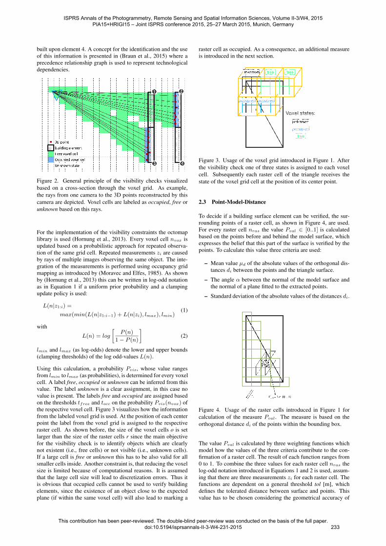
built upon element 4. A concept for the identification and the useof this information is presented in (Braun et al., 2015) where aprecedence relationship graph is used to represent technologicaldependencies.

Figure 2. General principle of the visibility checks visualizedbased on a cross-section through the voxel grid. As example,the rays from one camera to the 3D points reconstructed by thiscamera are depicted. Voxel cells are labeled as occupied, free orunknown based on this rays.

For the implementation of the visibility constraints the octomaplibrary is used (Hornung et al., 2013). Every voxel cell nvox isupdated based on a probabilistic approach for repeated observa-tion of the same grid cell. Repeated measurements zi are causedby rays of multiple images observing the same object. The inte-gration of the measurements is performed using occupancy gridmapping as introduced by (Moravec and Elfes, 1985). As shownby (Hornung et al., 2013) this can be written in log-odd notationas in Equation 1 if a uniform prior probability and a clampingupdate policy is used:

L(n|z1:i) =max(min(L(n|z1:i−1) + L(n|zi), lmax), lmin)

(1)

with

L(n) = log

[P (n)

1− P (n)

](2)

lmin and lmax (as log-odds) denote the lower and upper bounds(clamping thresholds) of the log odd-values L(n).

Using this calculation, a probability Pvis, whose value rangesfrom lmin to lmax (as probabilities), is determined for every voxelcell. A label free, occupied or unknown can be inferred from thisvalue. The label unknown is a clear assignment, in this case novalue is present. The labels free and occupied are assigned basedon the thresholds tfree and tocc on the probability Pvis(nvox) ofthe respective voxel cell. Figure 3 visualizes how the informationfrom the labeled voxel grid is used. At the position of each centerpoint the label from the voxel grid is assigned to the respectiveraster cell. As shown before, the size of the voxel cells o is setlarger than the size of the raster cells r since the main objectivefor the visibility check is to identify objects which are clearlynot existent (i.e., free cells) or not visible (i.e., unknown cells).If a large cell is free or unknown this has to be also valid for allsmaller cells inside. Another constraint is, that reducing the voxelsize is limited because of computational reasons. It is assumedthat the large cell size will lead to discretization errors. Thus itis obvious that occupied cells cannot be used to verify buildingelements, since the existence of an object close to the expectedplane (if within the same voxel cell) will also lead to marking a

raster cell as occupied. As a consequence, an additional measureis introduced in the next section.

Figure 3. Usage of the voxel grid introduced in Figure 1. Afterthe visibility check one of three states is assigned to each voxelcell. Subsequently each raster cell of the triangle receives thestate of the voxel grid cell at the position of its center point.

2.3 Point-Model-Distance

To decide if a building surface element can be verified, the sur-rounding points of a raster cell, as shown in Figure 4, are used.For every raster cell nras the value Pval ∈ [0..1] is calculatedbased on the points before and behind the model surface, whichexpresses the belief that this part of the surface is verified by thepoints. To calculate this value three criteria are used:

– Mean value µd of the absolute values of the orthogonal dis-tances di between the points and the triangle surface.

– The angle α between the normal of the model surface andthe normal of a plane fitted to the extracted points.

– Standard deviation of the absolute values of the distances di.

Figure 4. Usage of the raster cells introduced in Figure 1 forcalculation of the measure Pval. The measure is based on theorthogonal distance di of the points within the bounding box.

The value Pval is calculated by three weighting functions whichmodel how the values of the three criteria contribute to the con-firmation of a raster cell. The result of each function ranges from0 to 1. To combine the three values for each raster cell nras thelog-odd notation introduced in Equations 1 and 2 is used, assum-ing that there are three measurements zi for each raster cell. Thefunctions are dependent on a general threshold tol [m], whichdefines the tolerated distance between surface and points. Thisvalue has to be chosen considering the geometrical accuracy of



233

the points and the co-registration accuracy. For the evaluationof the angle deviation, the tolerance threshold tolα [◦] has to beintroduced to define the maximum allowable deviation that cancontribute to the verification of the raster cell. Deviations largerthan tolα,max receive the minimum value lmin as probability.The parameters lmin and lmax are the clamping thresholds (asused in Equation 1) and also define the maximum and minimumprobability for all three cases.Equation 3 models the weighting based on the mean value µd. Asmall mean value is necessary to confirm the surface. If the meanvalue is smaller than half of the threshold tol, it contributes withthe maximum probability. From this position the probability de-creases linearly to the minimum probability value at the positionof 1.5 tol:

P (nras|z1) =

P (µd) =

lmax if: µd < 0.5 · tolp1(µd) if: 0.5 · tol < µd < 1.5 · tollmin if: µd > 1.5 · tol

(3)

with

p1(µd) =lmin − lmax

tol· µd + 1.5 · lmax − 0.5 · lmin (4)

Equation 5 models the weighting considering the angle deviationα. Since only planar surfaces are examined if a triangle meshis used, a planar object with the same orientation is necessaryto confirm the triangle. Consequently α only contributes to con-firm the object if its value is smaller than tolα. The probabilitydecreases linearly from 0 degree to tolα, starting with the proba-bility 3/4 lmax for no deviation (cf. Equation 6).

P (nras|z2) =

P (α) =

p2a(α) if: α < tolα

p2b(α) if: tolα < α < tolα,max

lmin if: α > tolα,max

(5)

with

p2a(α) =0.5− 3

4lmax

tolα· α+

3

4lmax (6)

p2b(α) =lmin − 0.5

tolα,max − tolα· (α+ tolα) + 0.5 (7)

Finally, Equation 8 models the weighting considering the stan-dard deviation of the distances. Since a small standard deviationdoes not proof the existence of the correct object a small stan-dard deviation leads to a neutral weighting (= 0.5), but for largestandard deviations probabilities smaller than 0.5 are introduced.

P (nras|z3) =

P (σd) =

0.5 if: σd < tol

p3(σd) if: tol < σd < 2 · tollmin if: σd > 2 · tol

(8)

withp3(σd) =

lmin − 0.5

tol· σd + 1− lmin (9)

3. EXPERIMENT

3.1 Data

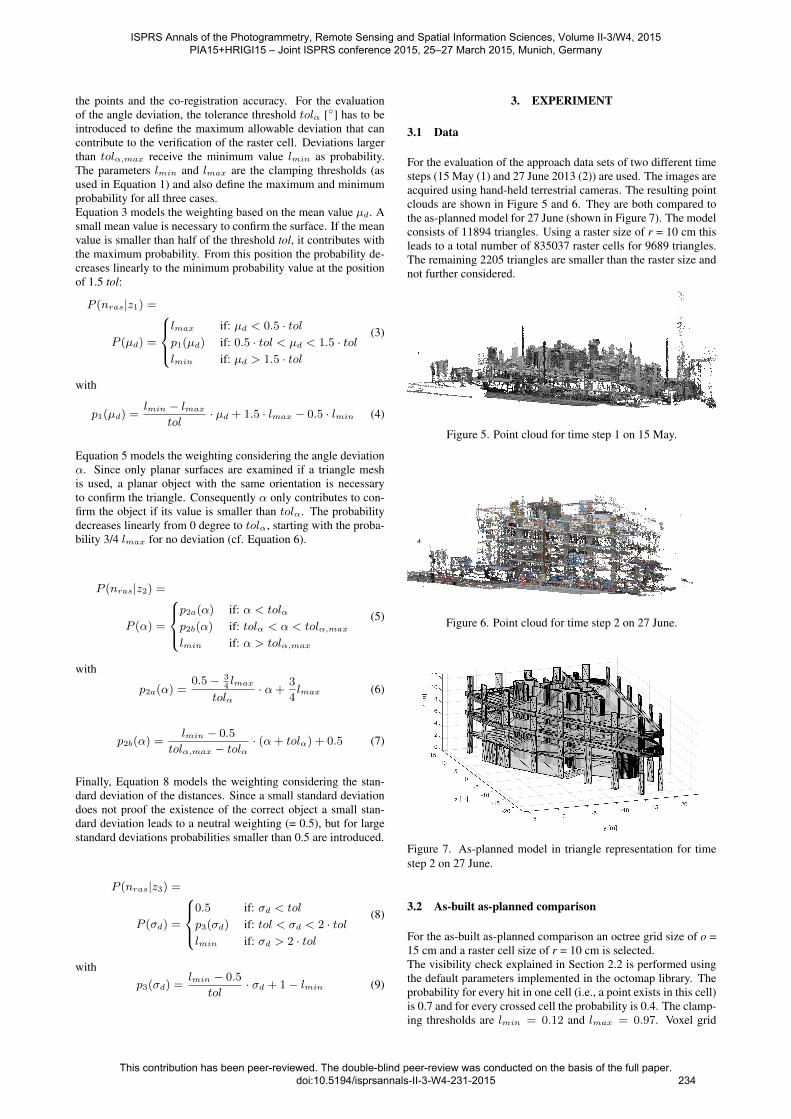
For the evaluation of the approach data sets of two different timesteps (15 May (1) and 27 June 2013 (2)) are used. The images areacquired using hand-held terrestrial cameras. The resulting pointclouds are shown in Figure 5 and 6. They are both compared tothe as-planned model for 27 June (shown in Figure 7). The modelconsists of 11894 triangles. Using a raster size of r = 10 cm thisleads to a total number of 835037 raster cells for 9689 triangles.The remaining 2205 triangles are smaller than the raster size andnot further considered.

Figure 5. Point cloud for time step 1 on 15 May.

Figure 6. Point cloud for time step 2 on 27 June.

Figure 7. As-planned model in triangle representation for timestep 2 on 27 June.

3.2 As-built as-planned comparison

For the as-built as-planned comparison an octree grid size of o =15 cm and a raster cell size of r = 10 cm is selected.The visibility check explained in Section 2.2 is performed usingthe default parameters implemented in the octomap library. Theprobability for every hit in one cell (i.e., a point exists in this cell)is 0.7 and for every crossed cell the probability is 0.4. The clamp-ing thresholds are lmin = 0.12 and lmax = 0.97. Voxel grid



234

cells having a probability Pvis smaller than tfree = 0.2 are la-beled as free and cells having a probability larger than tocc = 0.8are labeled as occupied. These thresholds are selected to ensurereliable labels what is motivated in the results section (3.3).As a result of the visibility check, building elements are extractedwhich can be clearly classified as not built or as not visible andwhich can be classified as potentially built. A building elementis regarded as not built if 90% of its raster cells are labeled asfree. A building element is regarded as not visible if 90% of itsraster cells are labeled as unknown. Finally a building elementis regarded as potentially built if at least 33% of the raster cellsare labeled as occupied. The elements classified as potentiallybuilt are further analyzed using the approach described in Section2.3 to calculate the value Pval for every raster cell. Therefore, abounding box size of b = 5 cm is used. The tolerance tol has to besmaller than the distance for the extraction of the points and is setto 2.5 cm. This value is inferred from the typical depth accuracywhich can be achieved with the selected acquisition geometry. Aloose threshold for the angle deviation tolα = 45◦ is selected dueto the fact that a plane is fitted to a small patch of the point cloud(10x10x10 cm). In combination with noisy points this may resultin large deviations even if the plane exists. The minimum andmaximum values for the probability are selected closely to zeroand one with lmin = 0.01 and lmax = 0.99 (consider that thesetwo values can be chosen differently for the visibility checks andthe calculation of Pval).A raster cell is accepted as verified if Pval > 0.5. Then the verifi-cation rate VR (Equation 10) can be calculated, which is the ratioof the verified raster cells to all raster cells of one triangle. Rastercells having the label unknown are excluded from that calcula-tion, so that only the visible elements of the triangles are takeninto account.

V R =

∑nras,verified∑

nras −∑nras,unknown

(10)

Finally, a threshold can be applied to decide if a building elementtriangle is verified as being built, or the verification rate can beassigned to every triangle. In the results shown in the next sec-tion every triangle is given the state built if the verification rate islarger than 50%. A summary of all states and their dependenciesis given in Table 1.

Table 1. Dependencies of states.

3.3 Results

In Figures 8 and 9 the results for the visibility checks are shown.All triangles marked in blue are labeled as not visible, the red tri-angles are labeled as not built and the green triangles are labeledas potentially built. In Table 2, the number of triangles for eachlabel are given. Triangles not classified as one of the states are inthe group rest and are not shown in the figures. The number oftriangles in this group is relatively large because the thresholdsare strict for the labels unknown and free. The strict threshold isused to ensure a reliable labeling for these two states. Since thethreshold on the percentage of occupied cells for the label poten-tially built is rather loose, the group rest is composed of triangles

which are built but not visible and which are not built. In the re-sults for time step 1 there is a large area marked as free since theas-planned state for the second time step is used. To be able tomark areas as free, points have to be reconstructed behind the pre-dicted planes, otherwise no rays pass through these planes. Thisexplains that the upper part in Figure 8 is labeled as unknown. Inboth cases the most triangles are labeled as unknown, what canmainly be ascribed to three reasons:

– The acquisition geometry only allows to see the triangleswhich face the cameras, all surfaces on the back are oc-cluded.

– Occlusions due to temporary and non modeled objects likeconstruction site fences or trailers, or the scaffolding.

– Objects inside the building cannot be seen due to two rea-son: (1) occlusion due to other objects, which have alreadybeen built; (2) not reconstructed areas because of the miss-ing illumination inside the building.

Figure 8. Result of the visibility checks for the point cloud oftime step 1 (Figure 5). Green triangles are labeled as potentiallybuilt, blue triangles are labeled as not visible and red triangles arelabeled as not built.

Figure 9. Result of the visibility checks for the point cloud oftime step 2 (Figure 6). Green triangles are labeled as potentiallybuilt, blue triangles are labeled as unknown and red triangles arelabeled as not built.

15 May 27 June

not built (red) 1281 13.2% 157 1.6%not visible (blue) 3360 34.7% 6742 69.6%pot. built (green) 871 9.0% 493 5.1%

rest 4177 43.1% 2297 23.7%

Table 2. Numerical results for the visibility checks: the numberof triangles for each class are given

For all triangles labeled as potentially built the verification rateis calculated and the label is changed to built if it is higher then50%. In Figure 10 the results for both time steps is depicted.All triangles labeled as potentially built in one of the both datasets (i.e., all green triangles from Figure 8 and 9) are shown, thecolored triangles are the one which are verified. The green tri-angles indicate the elements confirmed by the point cloud from



235

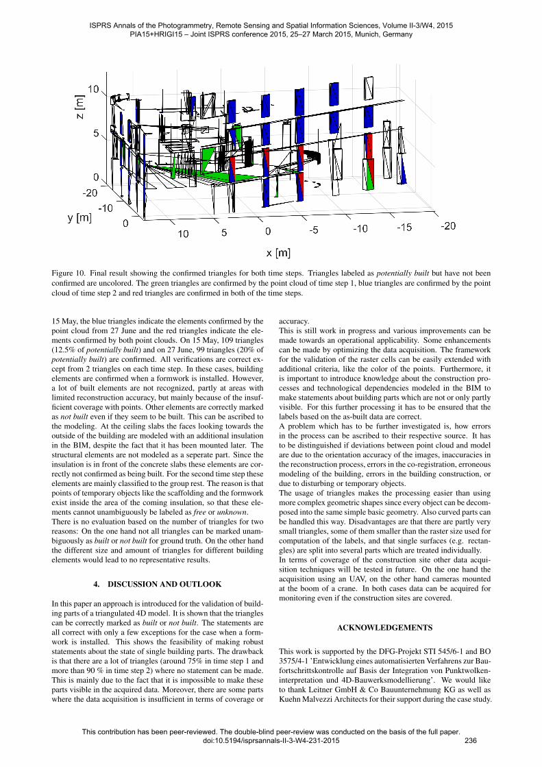
Figure 10. Final result showing the confirmed triangles for both time steps. Triangles labeled as potentially built but have not beenconfirmed are uncolored. The green triangles are confirmed by the point cloud of time step 1, blue triangles are confirmed by the pointcloud of time step 2 and red triangles are confirmed in both of the time steps.

15 May, the blue triangles indicate the elements confirmed by thepoint cloud from 27 June and the red triangles indicate the ele-ments confirmed by both point clouds. On 15 May, 109 triangles(12.5% of potentially built) and on 27 June, 99 triangles (20% ofpotentially built) are confirmed. All verifications are correct ex-cept from 2 triangles on each time step. In these cases, buildingelements are confirmed when a formwork is installed. However,a lot of built elements are not recognized, partly at areas withlimited reconstruction accuracy, but mainly because of the insuf-ficient coverage with points. Other elements are correctly markedas not built even if they seem to be built. This can be ascribed tothe modeling. At the ceiling slabs the faces looking towards theoutside of the building are modeled with an additional insulationin the BIM, despite the fact that it has been mounted later. Thestructural elements are not modeled as a seperate part. Since theinsulation is in front of the concrete slabs these elements are cor-rectly not confirmed as being built. For the second time step theseelements are mainly classified to the group rest. The reason is thatpoints of temporary objects like the scaffolding and the formworkexist inside the area of the coming insulation, so that these ele-ments cannot unambiguously be labeled as free or unknown.There is no evaluation based on the number of triangles for tworeasons: On the one hand not all triangles can be marked unam-biguously as built or not built for ground truth. On the other handthe different size and amount of triangles for different buildingelements would lead to no representative results.

4. DISCUSSION AND OUTLOOK

In this paper an approach is introduced for the validation of build-ing parts of a triangulated 4D model. It is shown that the trianglescan be correctly marked as built or not built. The statements areall correct with only a few exceptions for the case when a form-work is installed. This shows the feasibility of making robuststatements about the state of single building parts. The drawbackis that there are a lot of triangles (around 75% in time step 1 andmore than 90 % in time step 2) where no statement can be made.This is mainly due to the fact that it is impossible to make theseparts visible in the acquired data. Moreover, there are some partswhere the data acquisition is insufficient in terms of coverage or

accuracy.This is still work in progress and various improvements can bemade towards an operational applicability. Some enhancementscan be made by optimizing the data acquisition. The frameworkfor the validation of the raster cells can be easily extended withadditional criteria, like the color of the points. Furthermore, itis important to introduce knowledge about the construction pro-cesses and technological dependencies modeled in the BIM tomake statements about building parts which are not or only partlyvisible. For this further processing it has to be ensured that thelabels based on the as-built data are correct.A problem which has to be further investigated is, how errorsin the process can be ascribed to their respective source. It hasto be distinguished if deviations between point cloud and modelare due to the orientation accuracy of the images, inaccuracies inthe reconstruction process, errors in the co-registration, erroneousmodeling of the building, errors in the building construction, ordue to disturbing or temporary objects.The usage of triangles makes the processing easier than usingmore complex geometric shapes since every object can be decom-posed into the same simple basic geometry. Also curved parts canbe handled this way. Disadvantages are that there are partly verysmall triangles, some of them smaller than the raster size used forcomputation of the labels, and that single surfaces (e.g. rectan-gles) are split into several parts which are treated individually.In terms of coverage of the construction site other data acqui-sition techniques will be tested in future. On the one hand theacquisition using an UAV, on the other hand cameras mountedat the boom of a crane. In both cases data can be acquired formonitoring even if the construction sites are covered.

ACKNOWLEDGEMENTS

This work is supported by the DFG-Projekt STI 545/6-1 and BO3575/4-1 ’Entwicklung eines automatisierten Verfahrens zur Bau-fortschrittskontrolle auf Basis der Integration von Punktwolken-interpretation und 4D-Bauwerksmodellierung’. We would liketo thank Leitner GmbH & Co Bauunternehmung KG as well asKuehn Malvezzi Architects for their support during the case study.



236

We also would like to thank Konrad Eder for his support duringthe data acquisition.

REFERENCES

Bosche, F., 2010. Automated recognition of 3d cad model objectsin laser scans and calculation of as-built dimensions for dimen-sional compliance control in construction. Advanced EngineeringInformatics 24(1), pp. 107–118.

Bosche, F. and Haas, C. T., 2008. Automated retrieval of 3dcad model objects in construction range images. Automation inConstruction 17(4), pp. 499–512.

Braun, A., Borrmann, A., Tuttas, S. and Stilla, U., 2014. To-wards automated construction progress monitoring using bim-based point cloud processing. In: A. Mahdavi, B. Martens andR. Scherer (eds), ECPPM 2014, CRC Press, pp. 101–107.

Braun, A., Borrmann, A., Tuttas, S. and Stilla, U., 2015. A con-cept for automated construction progress monitoring using bim-based geometric constraints and photogrammetric point clouds.Journal of Information Technology in Construction 20, pp. 68 –79.

Brilakis, I., Fathi, H. and Rashidi, A., 2011. Progressive 3d re-construction of infrastructure with videogrammetry. Automationin Construction 20(7), pp. 884–895.

Fathi, H. and Brilakis, I., 2011. Automated sparse 3d point cloudgeneration of infrastructure using its distinctive visual features.Advanced Engineering Informatics 25(4), pp. 760–770.

Golparvar-Fard, M., Bohn, J., Teizer, J., Savarese, S. and Pe?a-Mora, F., 2011a. Evaluation of image-based modeling and laserscanning accuracy for emerging automated performance moni-toring techniques. Automation in Construction 20(8), pp. 1143–1155.

Golparvar-Fard, M., Pena Mora, F. and Savarese, S., 2012. Au-tomated progress monitoring using unordered daily constructionphotographs and ifc-based building information models. Journalof Computing in Civil Engineering.

Golparvar-Fard, M., Pena-Mora, F. and Savarese, S., 2011b.Monitoring changes of 3d building elements from unorderedphoto collections. In: Computer Vision Workshops (ICCV Work-shops), 2011 IEEE International Conference on, pp. 249–256.

Hornung, A., Wurm, K., Bennewitz, M., Stachniss, C. and Bur-gard, W., 2013. Octomap: an efficient probabilistic 3d map-ping framework based on octrees. Autonomous Robots 34(3),pp. 189–206.

Ibrahim, Y. M., Lukins, T. C., Zhang, X., Trucco, E. and Kaka,A. P., 2009. Towards automated progress assessment of work-package components in construction projects using computer vi-sion. Advanced Engineering Informatics 23(1), pp. 93–103.

Kim, C., Kim, B. and Kim, H., 2013a. 4d cad model updatingusing image processing-based construction progress monitoring.Automation in Construction 35, pp. 44–52.

Kim, C., Son, H. and Kim, C., 2013b. Automated constructionprogress measurement using a 4d building information model and3d data. Automation in Construction 31, pp. 75–82.

Moravec, H. P. and Elfes, A., 1985. High resolution maps fromwide angle sonar. In: Robotics and Automation. Proceedings.1985 IEEE International Conference on, Vol. 2, pp. 116–121.

Rankohi, S. and Waugh, L., 2014. Image-based modeling ap-proaches for projects status comparison. In: CSCE 2014 GeneralConference.

Rashidi, A., Brilakis, I. and Vela, P., 2014. Generating absolute-scale point cloud data of built infrastructure scenes using amonocular camera setting. Journal of Computing in Civil En-gineering pp. 04014089–1 – 04014089–12.

Son, H. and Kim, C., 2010. 3d structural component recognitionand modeling method using color and 3d data for constructionprogress monitoring. Automation in Construction 19(7), pp. 844–854.

Turkan, Y., Bosche, F., Haas, C. and Haas, R., 2013. Towardautomated earned value tracking using 3d imaging tools. Journalof Construction Engineering and Management 139(4), pp. 423–433.

Turkan, Y., Bosche, F., Haas, C. T. and Haas, R., 2012. Auto-mated progress tracking using 4d schedule and 3d sensing tech-nologies. Automation in Construction 22, pp. 414–421.

Turkan, Y., Bosche, F., Haas, C. T. and Haas, R., 2014. Track-ing of secondary and temporary objects in structural concretework. Construction Innovation: Information, Process, Manage-ment 14(2), pp. 145–167.

Tuttas, S., Braun, A., Borrmann, A. and Stilla, U., 2014a. Com-parison of photogrammetric point clouds with bim building ele-ments for construction progress monitoring. In: Int. Arch. Pho-togramm. Remote Sens. Spatial Inf. Sci., Vol. XL-3, CopernicusPublications, pp. 341–345. ISPRS Archives.

Tuttas, S., Braun, A., Borrmann, A. and Stilla, U., 2014b.Konzept zur automatischen baufortschrittskontrolle durch in-tegration eines building information models und photogram-metrisch erzeugten punktwolken. In: E. Seyfert, E. G?lch,C. Heipke, J. Schiewe and M. Sester (eds), Gemeinsame Tagung2014 der DGfK, der DGPF, der GfGI und des GiN, pp. 363–372.

Zhang, C. and Arditi, D., 2013. Automated progress control us-ing laser scanning technology. Automation in Construction 36,pp. 108–116.



237

validation of bim components by photogrammetric

Documents