42

Chapter 5

Photogrammetric Modeling

This chapter presents our photogrammetric modeling method, in which the computer de-

termines the parameters of a hierarchical model to reconstruct the architectural scene. Since our

method has the computer solve for a small number of model parameters rather than a large number

of vertex coordinates, the method is robust and requires a relatively small amount of user interaction.

The modeling method also computes the positions from which the photographs were taken.

We have implemented this method in Facade, an easy-to-use interactive modeling pro-

gram that allows the user to construct a geometric model of a scene from digitized photographs. We

first overview Facade from the point of view of the user, then we describe our model representation,

and then we explain our reconstruction algorithm. Lastly, we present results from using Facade to

reconstruct several architectural scenes.

43

(a) (b)

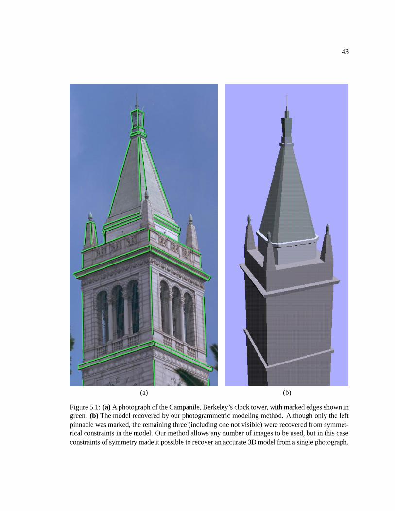
Figure 5.1: (a) A photograph of the Campanile, Berkeley’s clock tower, with marked edges shown ingreen. (b) The model recovered by our photogrammetric modeling method. Although only the leftpinnacle was marked, the remaining three (including one not visible) were recovered from symmet-rical constraints in the model. Our method allows any number of images to be used, but in this caseconstraints of symmetry made it possible to recover an accurate 3D model from a single photograph.

44

(a) (b)

Figure 5.2: (a) The accuracy of the model is verified by reprojecting it into the original photographthrough the recovered camera position. (b) A synthetic view of the Campanile generated using theview-dependent texture-mapping method described in Section 6. A real photograph from this posi-tion would be difficult to take since the camera position is 250 feet above the ground.

45

5.1 Overview of the Facade photogrammetric modeling system

Constructing a geometric model of an architectural scene using Facade is an incremental

and straightforward process. Typically, the user selects a small number of photographs to begin with,

and models the scene one piece at a time. The user may refine the model and include more images

in the project until the model meets the desired level of detail.

Fig. 5.1(a) and (b) shows the two types of windows used in Facade: image viewers and

model viewers. The user instantiates the components of the model, marks edges in the images, and

corresponds the edges in the images to the edges in the model. When instructed, Facade computes

the sizes and relative positions of the model components that best fit the edges marked in the pho-

tographs.

Components of the model, called blocks, are parameterized geometric primitives such as

boxes, prisms, and surfaces of revolution. A box, for example, is parameterized by its length, width,

and height. The user models the scene as a collection of such blocks, creating new block classes as

desired. Of course, the user does not need to specify numerical values for the blocks’ parameters,

since these are recovered by the program.

The user may choose to constrain the sizes and positions of any of the blocks. In Fig.

5.1(b), most of the blocks have been constrained to have equal length and width. Additionally, the

four pinnacles have been constrained to have the same shape. Blocks may also be placed in con-

strained relations to one other. For example, many of the blocks in Fig. 5.1(b) have been constrained

to sit centered and on top of the block below. Such constraints are specified using a graphical 3D in-

terface. When such constraints are provided, they are used to simplify the reconstruction problem.

Lastly, the user may set any parameter in the model to be a constant value - this needs to be done for

46

at least one parameter of the model to provide the model’s scale.

The user marks edge features in the images using a point-and-click interface; a gradient-

based technique as in [29] can be used to align the edges with sub-pixel accuracy. We use edge rather

than point features since they are easier to localize and less likely to be completely obscured. Only

a section of each edge needs to be marked, making it possible to use partially visible edges. For

each marked edge, the user also indicates the corresponding edge in the model. Generally, accu-

rate reconstructions are obtained if there are as many correspondences in the images as there are free

camera and model parameters. Thus, Facade reconstructs scenes accurately even when just a portion

of the visible edges and marked in the images, and when just a portion of the model edges are given

correspondences. Marking edges is particularly simple because Facade does not require that the end-

points of the edges be correctly specified; the observed and marked edges need only be coincident

and parallel.

At any time, the user may instruct the computer to reconstruct the scene. The computer

then solves for the parameters of the model that cause it to align with the marked features in the

images. During the reconstruction, the computer computes and displays the locations from which

the photographs were taken. For simple models consisting of just a few blocks, a full reconstruction

takes only a few seconds; for more complex models, it can take a few minutes. For this reason, the

user can instruct the computer to employ faster but less precise reconstruction algorithms (see Sec.

5.4.3) during the intermediate stages of modeling.

To verify the the accuracy of the recovered model and camera positions, Facade can project

the model into the original photographs. Typically, the projected model deviates from the photographs

by less than a pixel. Fig. 5.2(a) shows the results of projecting the edges of the model in Fig. 5.1(b)

47

into the original photograph.

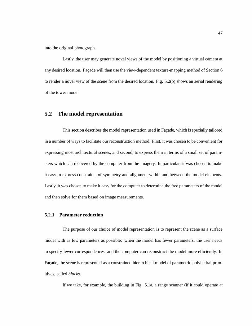
Lastly, the user may generate novel views of the model by positioning a virtual camera at

any desired location. Facade will then use the view-dependent texture-mapping method of Section 6

to render a novel view of the scene from the desired location. Fig. 5.2(b) shows an aerial rendering

of the tower model.

5.2 The model representation

This section describes the model representation used in Facade, which is specially tailored

in a number of ways to facilitate our reconstruction method. First, it was chosen to be convenient for

expressing most architectural scenes, and second, to express them in terms of a small set of param-

eters which can recovered by the computer from the imagery. In particular, it was chosen to make

it easy to express constraints of symmetry and alignment within and between the model elements.

Lastly, it was chosen to make it easy for the computer to determine the free parameters of the model

and then solve for them based on image measurements.

5.2.1 Parameter reduction

The purpose of our choice of model representation is to represent the scene as a surface

model with as few parameters as possible: when the model has fewer parameters, the user needs

to specify fewer correspondences, and the computer can reconstruct the model more efficiently. In

Facade, the scene is represented as a constrained hierarchical model of parametric polyhedral prim-

itives, called blocks.

If we take, for example, the building in Fig. 5.1a, a range scanner (if it could operate at

48

such a distance) or stereo algorithm (if there were another photo) would model the scene by acquir-

ing a depth measurement for each of the hundreds of thousands of pixels in the image. This approach

ignores the constrained structure of the architecture, and instead treats the scene as a cloud of points

with hundreds of thousands of individual measurements. If we were to represent the scene as a col-

lection of one hundred or so polygons, we would only need to recover the 3D coordinates of each

of the polygon edges, taking only a thousand or so values to represent the scene. Thus, by using

a higher-level representation, we are able to represent the same scene with less information. If we

can find a way to recover this information from the imagery, the reconstruction process can be much

simpler.

Taking this line of reasoning further, we can see that the scene is not a random collection of

oddly oriented polygons, but rather that it has a very regular structure. This regular structure can be

exploited by using a higher-level model representation, one that models the building in terms of its

salient architectural dimensions rather than the coordintates of its polyhedral vertices. By using this

high-level representation that we are about to describe, we can represent the scene with just tens of

parameters rather than thousands of vertex coordinates. Our reconstruction method is able to solve

directly for these tens of parameters, which greatly simplifies the reconstruction problem and reduces

by two orders of magnitude the number of image correspondences necessary to reconstruct the scene.

As one result, our method was able to robustly recover a full three-dimensional model of a clock

tower from just seventy marked edges in the single photograph in Fig. 5.1a.

5.2.2 Blocks

In Facade, the model consists of a hierarchy of blocks. Each block has a small set of scalar

parameters which serve to define its size and shape. Each coordinate of each vertex of the block

49

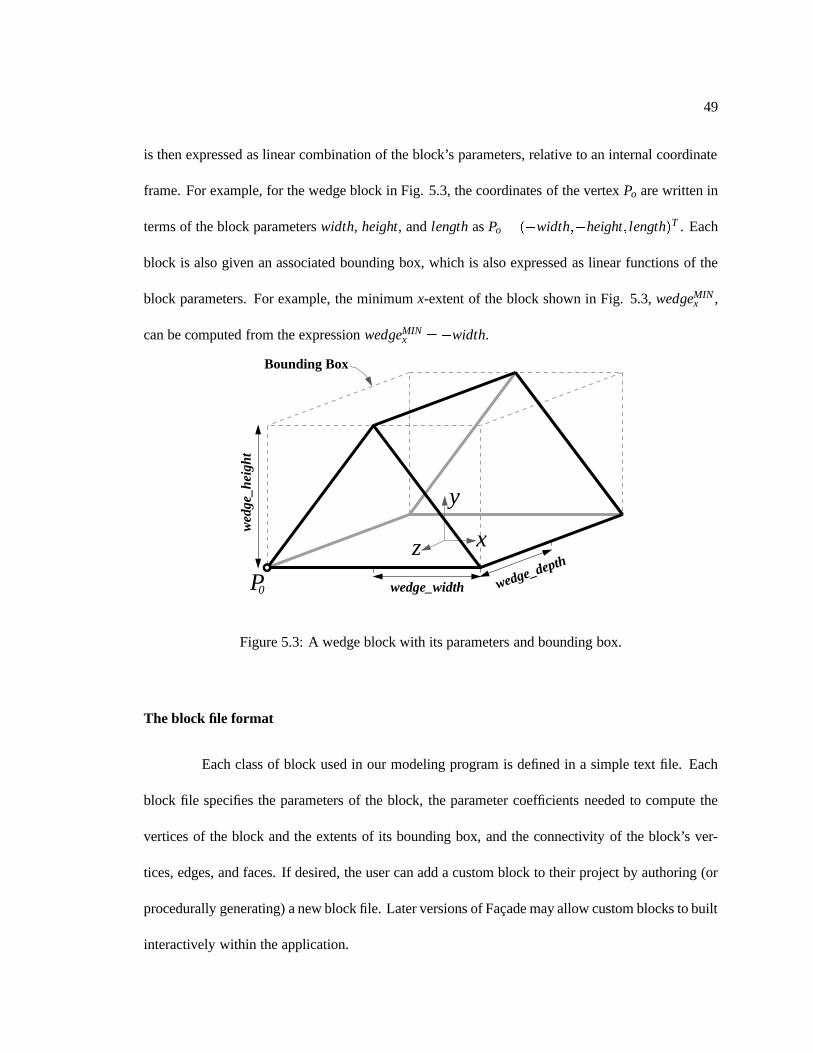
is then expressed as linear combination of the block’s parameters, relative to an internal coordinate

frame. For example, for the wedge block in Fig. 5.3, the coordinates of the vertex Po are written in

terms of the block parameters width, height, and length as Po = (�width;�height; length)T . Each

block is also given an associated bounding box, which is also expressed as linear functions of the

block parameters. For example, the minimum x-extent of the block shown in Fig. 5.3, wedgeMINx ,

can be computed from the expression wedgeMINx =�width.

y

z x

wedge_width

wed

ge_h

eigh

t

wedge_depth

Bounding Box

P0

Figure 5.3: A wedge block with its parameters and bounding box.

The block file format

Each class of block used in our modeling program is defined in a simple text file. Each

block file specifies the parameters of the block, the parameter coefficients needed to compute the

vertices of the block and the extents of its bounding box, and the connectivity of the block’s ver-

tices, edges, and faces. If desired, the user can add a custom block to their project by authoring (or

procedurally generating) a new block file. Later versions of Facade may allow custom blocks to built

interactively within the application.

50

roof

first_storey

y

xz

ground_plane

y

xz

y

xz y

xzentrance

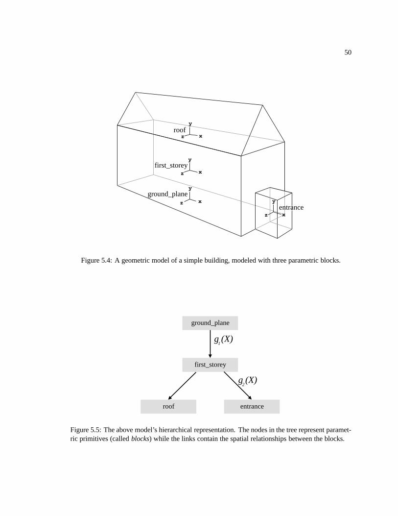
Figure 5.4: A geometric model of a simple building, modeled with three parametric blocks.

ground_plane

first_storey

roof entrance

g (X)1

g (X)2

Figure 5.5: The above model’s hierarchical representation. The nodes in the tree represent paramet-ric primitives (called blocks) while the links contain the spatial relationships between the blocks.

51

5.2.3 Relations (the model hierarchy)

The blocks in Facade are organized in a hierarchical tree structure as shown in Fig. 5.5.

Each node of the tree represents an individual block, while the links in the tree contain the spatial rela-

tionships between blocks, called relations. Similar hierarchical representations are used throughout

computer graphics to model complicated objects in terms of simple geometrical primitives.

The relation between a block and its parent is most generally represented as a rotation ma-

trix R and a translation vector t. This representation requires six parameters: three each for R and t.

In architectural scenes, however, the relationship between two blocks usually has a simple form that

can be represented with fewer parameters, and Facade allows the user to build such constraints on R

and t into the model. The rotation R between a block and its parent can be specified in one of three

ways:

1. An unconstrained rotation (three parameters)

2. A rotation about a particular coordinate axis (one parameter)

3. No rotation, or a fixed rotation (zero parameters)

Likewise, Facade allows for constraints to be placed on each component of the translation

vector t. Specifically, the user can constrain the bounding boxes of two blocks to align themselves in

some manner along each dimension. For example, in order to ensure that the roof block in Fig. 5.4

lies on top of the first story block, the user can require that the maximum y extent of the first story

block be equal to the minimum y extent of the roof block. With this constraint, the translation along

the y axis is computed (ty = ( f irst storyMAXy � roo f MIN

y )) rather than represented as a parameter of

the model.

52

Modeling the spatial relationships between blocks in the hierarchy with specialized forms

of translation and rotation serves to reduce the number of parameters in the model, since there is no

longer a full six-degree-of-freedom transformation between each block and its parent. In fact, for

most components of architecture, it is possible to completely constrain the translation and rotation

of a block with respect to its parent in terms of their bounding boxes. For the campanile model, in

fact, each of the twenty-two blocks is so constrained, representing the elimination of 22� 6 = 132

parameters from the model representation.

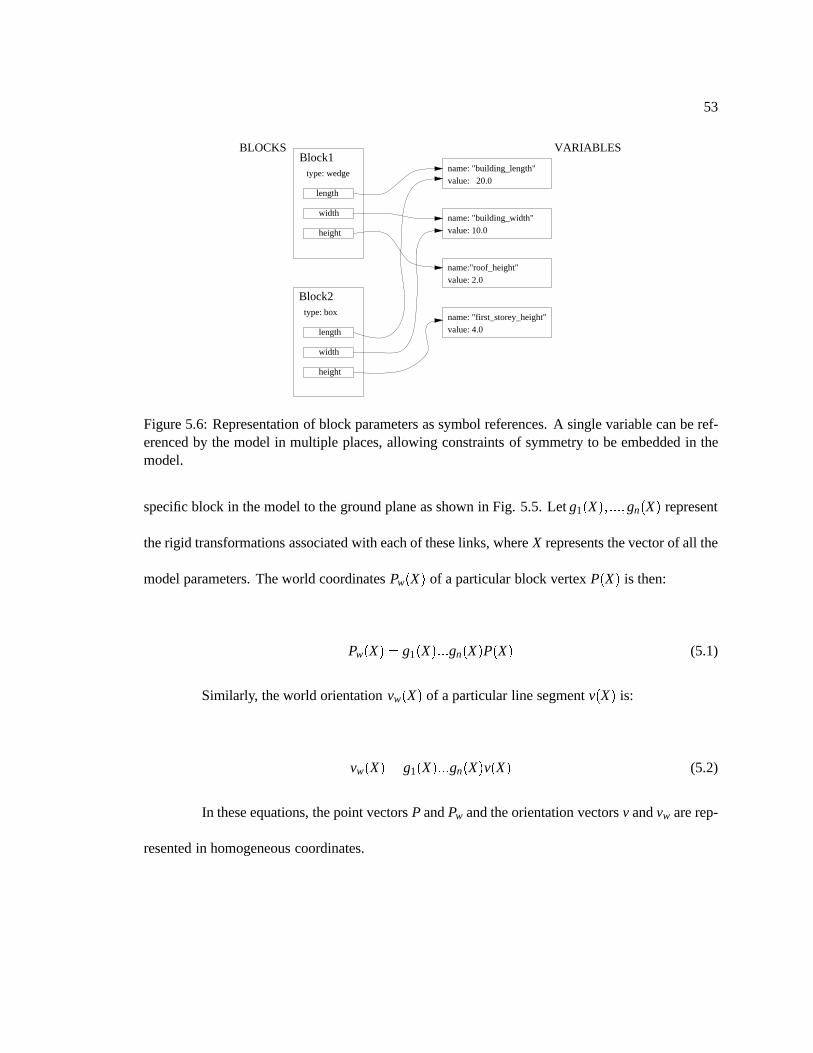
5.2.4 Symbol references

Each parameter of each instantiated block is actually a reference to a named symbolic vari-

able, as illustrated in Fig. 5.6. As a result, two parameters of different blocks (or of the same block)

can be equated by having each parameter reference the same symbol. This facility allows the user

to equate two or more of the dimensions in a model, which makes modeling symmetrical blocks

and repeated structure more convenient. This is used in several places in the Campanile model (Fig.

5.1b); most blocks have their north-south and east-west dimensions identified to the same parameter

to force square cross-sections, and the four pinnacles all share their dimensions. Importantly, these

constraints reduce the number of degrees of freedom in the model, which, as we will show, simplifies

the structure recovery problem. In the case of the Campanile model, there are just thirty-three free

parameters.

5.2.5 Computing edge positions using the hierarchical structure

Once the blocks and their relations have been parameterized, it is straightforward to derive

expressions for the world coordinates of the block vertices. Consider the set of edges which link a

53

Block2

Block1BLOCKS

height

length

type: wedge

width

height

width

length

type: box

name: "building_width"value: 10.0

value: 20.0name: "building_length"

value: 2.0

value: 4.0name: "first_storey_height"

name:"roof_height"

VARIABLES

Figure 5.6: Representation of block parameters as symbol references. A single variable can be ref-erenced by the model in multiple places, allowing constraints of symmetry to be embedded in themodel.

specific block in the model to the ground plane as shown in Fig. 5.5. Let g1(X); :::;gn(X) represent

the rigid transformations associated with each of these links, where X represents the vector of all the

model parameters. The world coordinates Pw(X) of a particular block vertex P(X) is then:

Pw(X) = g1(X):::gn(X)P(X) (5.1)

Similarly, the world orientation vw(X) of a particular line segment v(X) is:

vw(X) = g1(X):::gn(X)v(X) (5.2)

In these equations, the point vectors P and Pw and the orientation vectors v and vw are rep-

resented in homogeneous coordinates.

54

5.2.6 Discussion

Modeling the scene with polyhedral blocks, as opposed to points, line segments, surface

patches, or polygons, is advantageous for a number of reasons:

� Most architectural scenes are well modeled by an arrangement of geometric primitives.

� Blocks implicitly contain common architectural elements such as parallel lines and right an-

gles.

� Manipulating block primitives is convenient since they are at a suitably high level of abstrac-

tion; individual features such as points and lines are less manageable.

� A surface model of the scene is readily obtained from the blocks, so there is no need to infer

surfaces from discrete features.

� Modeling in terms of blocks and relationships greatly reduces the number of parameters that

the reconstruction algorithm needs to recover.

The last point is crucial to the robustness of our reconstruction algorithm and the viability

of our modeling system, and is illustrated best with an example. The model in Fig. 5.1 is parame-

terized by just 33 variables (the unknown camera position adds six more). If each block in the scene

were unconstrained (in its dimensions and position), the model would have 240 parameters; if each

line segment in the scene were treated independently, the model would have 2,896 parameters. This

reduction in the number of parameters greatly enhances the robustness and efficiency of the method

as compared to traditional structure from motion algorithms. Lastly, since the number of correspon-

dences needed to suitably overconstrain the optimization is roughly proportional to the number of

55

parameters in the model, this reduction means that the number of correspondences required of the

user is manageable.

5.3 Facade’s user interface

5.3.1 Overview

The Facade system is a graphical user interface application written in C++. It uses the IRIS

GL graphics library for its interactive 2D and 3D graphics and Mark Overmars’ FORMS library for

the dialog boxes. Facade makes it possible for the user to:

� Load in the images of the scene that is to be reconstructed

� Perform radial distortion correction on images, and specify camera parameters

� Mark features (points, edges, contours) in the images

� Instantiate and constrain the components of the model

� Form correspondences between components of the model and features in the photographs

� Automatically recover the scene and the camera locations based on the correspondences

� Inspect the model and the recovered camera locations

� Verify the model accuracy by projecting the model into the recovered cameras

� Output the geometry of the model in VRML (Virtual Reality Modeling Language) format

� Render the scene and create animations using various forms of texture mapping, including

view-dependent texture mapping (Chapter 6)

56

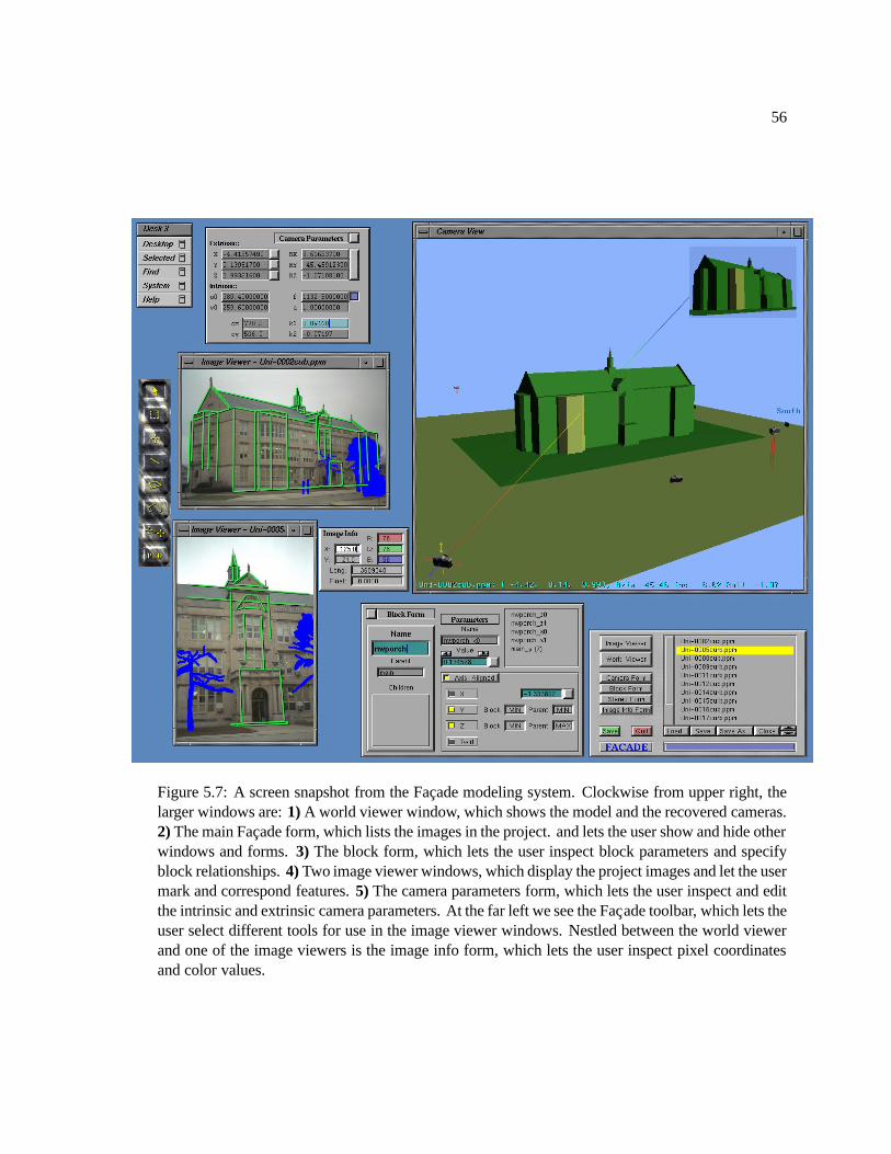
Figure 5.7: A screen snapshot from the Facade modeling system. Clockwise from upper right, thelarger windows are: 1) A world viewer window, which shows the model and the recovered cameras.2) The main Facade form, which lists the images in the project. and lets the user show and hide otherwindows and forms. 3) The block form, which lets the user inspect block parameters and specifyblock relationships. 4) Two image viewer windows, which display the project images and let the usermark and correspond features. 5) The camera parameters form, which lets the user inspect and editthe intrinsic and extrinsic camera parameters. At the far left we see the Facade toolbar, which lets theuser select different tools for use in the image viewer windows. Nestled between the world viewerand one of the image viewers is the image info form, which lets the user inspect pixel coordinatesand color values.

57

� Recover additional geometric detail from the model using model-based stereo (Chapter 7)

5.3.2 A Facade project

Facade saves a reconstruction project in a special text file, called save.facade by de-

fault. The project file stores the list of images used in the project (referenced by filename), and for

each image it stores the associated intrinsic and extrinsic camera parameters. For each image it also

stores a list of its marked features, which are indexed so that they may be referenced by the model.

The file then stores the model hierarchy. Each block is written out in depth-first order as it

appears in the model tree. For each block, its template file (its “.block” file name) and its parameter

values are written, followed by the type and parameters of its relationship to its parent. Then, for each

edge, a list of image feature indices is written to store the correspondences between the model and

the images.

5.3.3 The windows and what they do

Facade uses two principal types of windows – image viewers and world viewers – plus sev-

eral forms created with the FORMS library. Fig. 5.7 shows a screen snapshot of the Facade system

with its various windows and dialog boxes. These windows are described in the following sections.

The main window

The main Facade form displays a list of the images used in the project, and allows the user

to load new images and save renderings generated by the program. The user also uses this form to

create new image and world viewer windows, and to bring up the forms for inspecting and editing

the properties of blocks and cameras. The main window also allows the user to save the current state

58

of the project and exit the program.

The image viewer windows

Viewing images Images, once loaded into the project, are viewed through image viewer windows.

There can be any number of image viewers, and any viewer can switch to view any image. The

middle mouse button is used to pan the image around in the window, and the user can zoom in or

out of the image by clicking the left and right mouse buttons while holding down the middle mouse

button. The image zooming and scrolling functions were made to be very responsive by making

direct calls to the pixmap display hardware.

Marking features The image viewers are principally used to mark and correspond features in the

images. Tools for marking points, line segments, and image contours are provided by the toolbar. As

a result of the button-chording image navigation and zooming technique, it is convenient to position

features with sub-pixel accuracy. The marked features are drawn overlaid on the image using shad-

owed, antialiased lines (Fig. 5.1a). A pointer tool allows the user to adjust the positions of features

once they are marked; features may also be deleted.

Forming correspondences Correspondences are made between features in the model (usually edges)

and features in the images by first clicking on a feature in the model (using a world viewer window)

and then clicking on the corresponding feature while holding down the shift key. The feature

changes to a different color to indicate that it has been corresponded. To verify correspondences, an

option in the image viewer pop-up menu allows the user to select a marked image feature and have

Facade select the corresponding part of the model.

59

Reprojecting the model An item in the image viewer pop-up menu projects the model into the

current image, through its corresponding camera geometry, and overlays the model edges on the im-

age (Fig. 5.2a). This feature can be used to check the accuracy of the reconstruction: if the model

edges align well with the user-drawn edges and the original picture, then the model is accurate. If

there is a particular part of the architecture that does not align well with the image, then the user can

check whether the right correspondences were made, or whether that piece of the architecture was

modeled properly.

The world viewer windows

The world viewer windows are used to view and manipulate the 3D model and to inspect

the recovered camera positions. The user can interactively move his or her viewpoint around the

model using the mouse.

Selecting cameras The world viewer in the upper right of Fig. 5.7 shows the high school model

in its finished state, and several of the recovered camera positions are visible. The camera in the

lower left of the viewer has been selected, and as a result the camera is drawn with manipulation

handles and the upper right of the world viewer shows the model as viewed through this camera. For

comparision, the image viewer to the left of the world viewer shows the original image corresponding

to this camera. If the camera form (see below) is active, then it numerically displays the selected

camera’s intrinsic and extrinsic information.

Selecting blocks The user may select a block in the model by clicking on it. In the figure, the

user has selected the block that models the northwest bay window of the building, and this block is

60

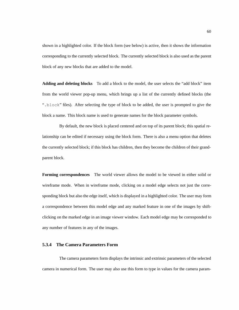
shown in a highlighted color. If the block form (see below) is active, then it shows the information

corresponding to the currently selected block. The currently selected block is also used as the parent

block of any new blocks that are added to the model.

Adding and deleting blocks To add a block to the model, the user selects the “add block” item

from the world viewer pop-up menu, which brings up a list of the currently defined blocks (the

“.block” files). After selecting the type of block to be added, the user is prompted to give the

block a name. This block name is used to generate names for the block parameter symbols.

By default, the new block is placed centered and on top of its parent block; this spatial re-

lationship can be edited if necessary using the block form. There is also a menu option that deletes

the currently selected block; if this block has children, then they become the children of their grand-

parent block.

Forming correspondences The world viewer allows the model to be viewed in either solid or

wireframe mode. When in wireframe mode, clicking on a model edge selects not just the corre-

sponding block but also the edge itself, which is displayed in a highlighted color. The user may form

a correspondence between this model edge and any marked feature in one of the images by shift-

clicking on the marked edge in an image viewer window. Each model edge may be corresponded to

any number of features in any of the images.

5.3.4 The Camera Parameters Form

The camera parameters form displays the intrinsic and extrinsic parameters of the selected

camera in numerical form. The user may also use this form to type in values for the camera param-

61

eters manually. The camera form in the upper left of Fig. 5.7 is displaying the information corre-

sponding to the selected camera indicated in the world viewer.

In typical use, the camera’s intrinsic parameters will be entered by the user after the cali-

bration process (Chapter 4) and the extrinsic values will be computed automatically by Facade. Al-

though the camera rotation is represented internally as a quaternion, for convenience the user inter-

face displays and receives the camera rotation value as its three Euler angles.

By clicking in the small boxes to the left of the entry fields, the camera rotation and each

one of its coordinates may individually be set to be treated as constants. When one of these parame-

ters is set to be constant, its value is not adjusted by the optimization process. This allows the system

to work with camera position data from GPS sensors or from motion-controled camera systems.

5.3.5 The Block Parameters form

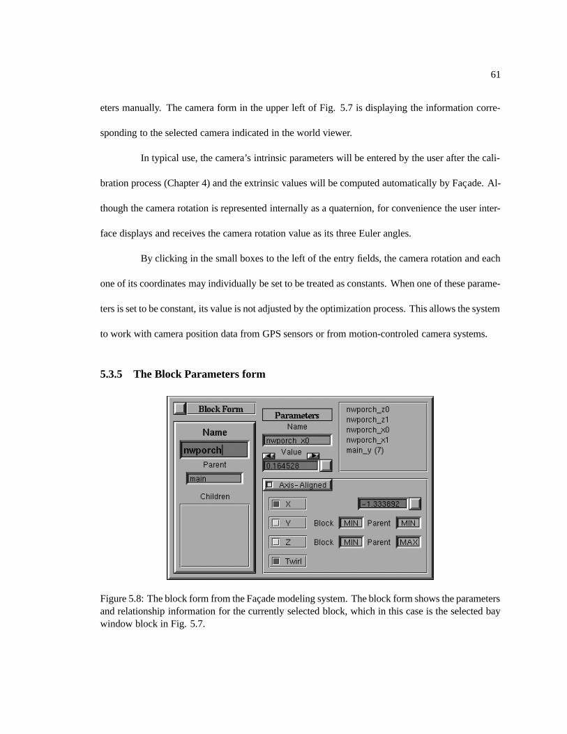
Figure 5.8: The block form from the Facade modeling system. The block form shows the parametersand relationship information for the currently selected block, which in this case is the selected baywindow block in Fig. 5.7.

62

The block parameters form is used to edit the selected block’s internal parameters and its

spatial relationship to its parent. It is with this form that most of the model building takes place.

The block form at the bottom center of Fig. 5.7 shows the information corresponding to the selected

northwest bay window block of the high school building.

Block names The left section of the block form shows the name of the current block, the name of

the current block’s parent block, and a list of the names of the block’s children. The block name may

be changed by typing a new name, and the parent of the block can be changed by typing in the name

of different parent block.

Block parameters The top right section of the block form is used to inspect and edit the block

parameters. The names of the block parameters are listed in the box on the right; these names are,

by default, the name of the block with a suffix that describes the parameter. For example, the height

of a box block named “main” would be called “main y” by default.

Clicking on one of the listed parameter names displays the parameter’s name and value in

the entry fields to the left. Using these entry fields, it is possible to rename the selected block parame-

ter, and to inspect or change the block parameter value. For convenience, the value may be increased

or decreased by ten percent using the arrow buttons above the parameter value field. Although the

block parameters are usually determined by the reconstruction algorithm, the ability to change the

values interactively is sometimes useful for adding hypothetical structures to the scene.

To the right of the parameter value field is a small square button, which may be clicked

into a down position to signify that the block parameter should be held constant and not computed

by the reconstruction algorithm. When a parameter is held constant, it is displayed in the list of block

63

parameter names in boldface type. Typically, at least one parameter of the model needs to be set to a

constant value to provide an absolute scale for the model. Setting parameters to be constant is also a

convenient way to include any available ground truth information (from survey data or architectural

plans) in the project.

Equating parameters The parameter name field can be used to rename any of a block’s param-

eters. The user can use this facility to force two or more parameters in the model to have the same

value. As discussed in Sec. 5.2.4, the model parameters are implemented as references to symbols

in a symbol table. When the user renames a parameter in a block to the name of another parameter

in the model (either of the same block or of a different block), Facade deletes the parameter symbol

corresponding to the current parameter and changes this parameter to reference the symbol with the

supplied name. At this point, the symbol will be referenced by two different parameter slots in the

model. The number of references to a given symbol is indicated in parentheses to the right of the

parameter’s name in the block parameter list.

As an example, in Fig. 5.8, the last parameter was originally named “nwporch y”, indicat-

ing that it specified the height of the block “nwporch”. The user renamed this parameter to “main y”,

which deleted the symbol corresponding to the parameter “nwporch y” and pointed this parame-

ter to the symbol corresponding to the height of the main box of the building. From the number in

parentheses to the right of the parameter name, we can see that the dimension “main y” is actually

referenced seven times in the model. Because of this, the reconstruction algorithm needed to solve

for six fewer parameters in order to reconstruct the building, which meant that significantly fewer

correspondences needed to be provided by the user.

Such use of symbol references can be used in myriad ways to take advantage of various

64

forms of symmetry in a scene. In the Campanile model (Fig. 5.1b), most of the blocks were con-

strained to be square in cross-section by equating the parameters corresponding to their lengths and

widths. The four pinnacles were not only constrained to be square in cross-section, but they were

constrained to all have the same dimensions. As a result, just three parameters were necessary to

represent the geometry of all four pinnacles. This made it possible to reconstruct all four pinnacles,

including the one not visible in back, from the edges of just one of the pinnacles (see Fig. 5.1a).

Specifying block relations The spatial relationship of a block to its parent is specified in the lower

right section of the block form. The translation between the block and its parent is specified in terms

of constraints on each of the translational coordinates, relative to the internal coordinate frame of

the parent block. In Fig. 5.8, the y component of the translation is specified so that the minimum

y-coordinate of the “nwporch” block is the same as the minimum y-coordinate of its parent block

“main”, which is the main box of the building. Thus, these two blocks will lie even with each other

at their bottoms. Similarly, the z coordinate of the relation has been constrained so that the minimum

z-coordinate of the “nwporch” block is coincident with the maximum z-coordinate of the “main”

block. This constrains the back of the “nwporch” block to lie flush up against the side of the “main”

block. These two blocks can be seen in the world viewer in Fig. 5.7.

The user has left the x-coordinate of the translation between the block and its parent un-

constrained, so Facade displays the value of the parameter corresponding to this translation. In this

case, the reconstruction algorithm has calculated that there is a translation of �1:33892 units along

the x-dimension between the block and its parent. This value entry field can be used to type in a new

value, or to set it to be a constant by clicking the box to the right of the field. Since the translational

components are in the coordinate system of the parent block, it is possible to line up a child block

65

flush with its parent even when the parent block is rotated with respect to world coordinates.

This section of the block form is also used to specify the type of rotation that exists between

the selected block and its parent. In this example, the “Axis-Aligned” button has been highlighted,

which causes the rotation of the selected block with respect to world coordinates to be the same as the

rotation of its parent. As a result, the two blocks are not allowed to rotate with respect to each other.

If the user had not clicked the “Axis-Aligned” button, the reconstruction algorithm would solve for

a full three-degree-of-freedom rotation between the two blocks.

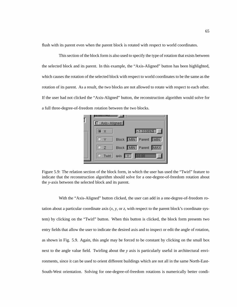
Figure 5.9: The relation section of the block form, in which the user has used the “Twirl” feature toindicate that the reconstruction algorithm should solve for a one-degree-of-freedom rotation aboutthe y-axis between the selected block and its parent.

With the “Axis-Aligned” button clicked, the user can add in a one-degree-of-freedom ro-

tation about a particular coordinate axis (x, y, or z, with respect to the parent block’s coordinate sys-

tem) by clicking on the “Twirl” button. When this button is clicked, the block form presents two

entry fields that allow the user to indicate the desired axis and to inspect or edit the angle of rotation,

as shown in Fig. 5.9. Again, this angle may be forced to be constant by clicking on the small box

next to the angle value field. Twirling about the y axis is particularly useful in architectural envi-

ronments, since it can be used to orient different buildings which are not all in the same North-East-

South-West orientation. Solving for one-degree-of-freedom rotations is numerically better condi-

66

tioned than solving for full three-degree-of-freedom rotations, so the “Twirl” feature should be used

instead of full rotation recovery whenever possible.

Of course, it is entirely optional for the user to provide any of these constraints on the pa-

rameters of the model and the spatial relationships between blocks — the reconstruction algorithm

is capable of reconstructing blocks in the general unconstrained case. However, these sorts of con-

straints are typically very apparent to the user, and the user interface makes it convenient for the user

to build such constraints into the model. The reconstruction algorithm implicitly makes use of these

constraints in that it simply solves for fewer free parameters. Since there are fewer parameters to

solve for, fewer marked correspondences are necessary for a robust solution.

5.3.6 Reconstruction options

The user tells Facade to reconstruct the scene via a special pop-up menu in the world viewer

window. By default, the reconstruction performs a three-stage optimization, which executes the two

phases of the initial estimate method (Sec. 5.4.3) followed by the full nonlinear optimization. For

convenience, the user may execute any of these stages independently. During the intermediate stages

of modeling, it is usually quite adequate to use only the initial estimate algorithms, saving the more

time-consuming nonlinear optimization for occasional use. Another time-saving reconstruction op-

tion allows the user to reconstruct only those model parameters corresponding to the currently se-

lected block and its descendants.

Even for the more complicated projects presented in this thesis, the time required to run

the reconstruction algorithms is very reasonable. For the high school model (Fig. 5.12), in the cur-

rent Facade implementation, running on a 200MHz Silicon Graphics Indigo2, the initial estimate

procedure takes less than a minute, and the full nonlinear optimization takes less than two minutes.

67

5.3.7 Other tools and features

There are several other useful features in the Facade system. First, the recovered model

geometry can be written out in VRML 1.0 or VRML 2.0 format to a “model.wrl” file. In VRML

form, the recovered geometry can be conveniently viewed over the internet. Second, the user can

have Facade generate synthetic views of the scene using the view-dependent texture mapping method

described in the next chapter. This is accomplished by positioning a novel camera in the scene and se-

lecting a menu option. Lastly, the user can choose any two images and have Facade generate detailed

depth maps for them using the model-based stereo method described in Chapter 7. Other specialized

rendering options can be used to make use of such depth maps to create detailed renderings.

5.4 The reconstruction algorithm

This section presents the reconstruction algorithm used in Facade, which optimizes over

the parameters of the model and the camera positions to make the model conform to the observed

edges in the images. The algorithm also uses a two-step initial estimate procedure that automatically

computes an estimate of the camera positions and the model parameters that is near the correct solu-

tion; this keeps the nonlinear optimization out of local minima and facilitates a swift convergence.

We first present the nonlinear objective function which is optimized in the reconstruction.

5.4.1 The objective function

Our reconstruction algorithm works by minimizing an objective function O that sums the

disparity between the projected edges of the model and the edges marked in the images, i.e. O =

∑Erri where Erri represents the disparity computed for edge feature i. Thus, the unknown model

68

parameters and camera positions are computed by minimizing O with respect to these variables. Our

system uses the the error function Erri from [47], described below.

!!!!!!!!!!!!!!!!!!!!!!!!!!!!!!!!!!!!!!!!!!!!!!!!!!!!!!!!!!!!!!!!!!!!!!!!!!!!!!!!!!!!!!!!!!!

image plane

3D line

m

v

image edge

y

−zx

y

−z

x

d World CoordinateSystem

<R, t>

Camera CoordinateSystem

predicted line:mxx + myy + mzf = 0

(x1, y1)

(x2, y2)

h1

h2

P(s)h(s) Observed edgesegment

!!!!

!!

(a) (b)

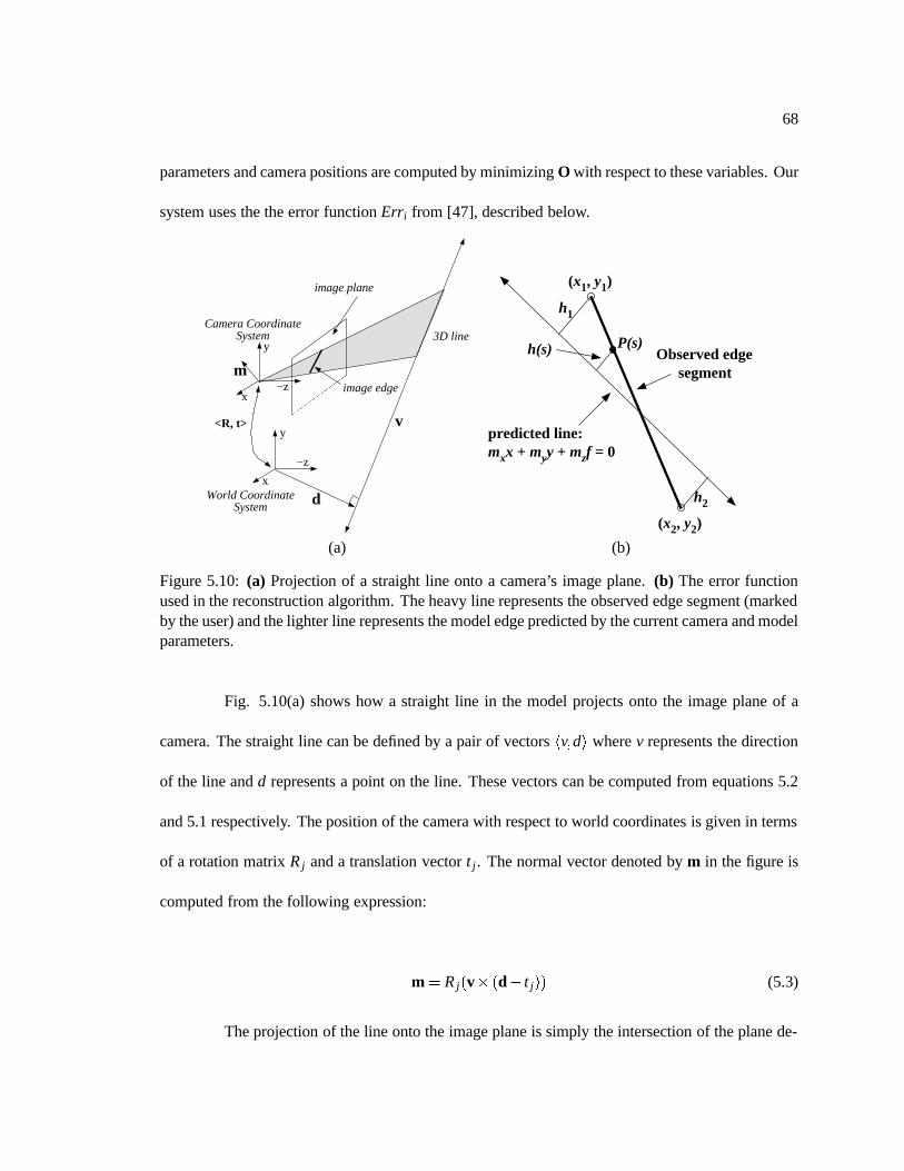
Figure 5.10: (a) Projection of a straight line onto a camera’s image plane. (b) The error functionused in the reconstruction algorithm. The heavy line represents the observed edge segment (markedby the user) and the lighter line represents the model edge predicted by the current camera and modelparameters.

Fig. 5.10(a) shows how a straight line in the model projects onto the image plane of a

camera. The straight line can be defined by a pair of vectors hv;di where v represents the direction

of the line and d represents a point on the line. These vectors can be computed from equations 5.2

and 5.1 respectively. The position of the camera with respect to world coordinates is given in terms

of a rotation matrix R j and a translation vector t j. The normal vector denoted by m in the figure is

computed from the following expression:

m = R j(v� (d� t j)) (5.3)

The projection of the line onto the image plane is simply the intersection of the plane de-

69

fined by m with the image plane, located at z =� f where f is the focal length of the camera. Thus,

the image edge is defined by the equation mxx+myy�mz f = 0.

Fig. 5.10(b) shows how the error between the observed image edge f(x1;y1);(x2;y2)g and

the predicted image line is calculated for each correspondence. Points on the observed edge segment

can be parameterized by a single scalar variable s 2 [0; l] where l =p

(x1 � x2)2 +(y1� y2)2 is the

length of the edge. We let h(s) be the function that returns the shortest distance from a point on the

segment, p(s), to the predicted edge.

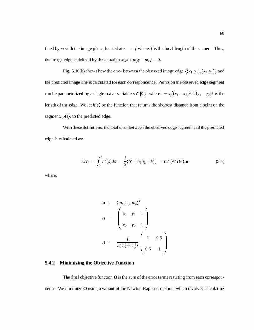
With these definitions, the total error between the observed edge segment and the predicted

edge is calculated as:

Erri =

Z l

0h2(s)ds =

l3(h2

1 +h1h2 +h22) = mT(AT BA)m (5.4)

where:

m = (mx;my;mz)T

A =

0BB@

x1 y1 1

x2 y2 1

1CCA

B =l

3(m2x +m2

y)

0BB@

1 0:5

0:5 1

1CCA

5.4.2 Minimizing the Objective Function

The final objective function O is the sum of the error terms resulting from each correspon-

dence. We minimize O using a variant of the Newton-Raphson method, which involves calculating

70

the gradient and Hessian of O with respect to the parameters of the camera and the model (see also

[41].) As we have shown, it is simple to construct symbolic expressions for m in terms of the un-

known model parameters. The minimization algorithm differentiates these expressions symbolically

to evaluate the gradient and Hessian after each iteration. The procedure is inexpensive since the ex-

pressions for d and v in Equations 5.2 and 5.1 have a particularly simple form.

One should note that some of the parameters over which it is necessary to optimize the

objective function are members of the rotation group SO(3); specifically, the camera rotations and

any rotations internal to the model. Since SO(3) is not isomorphic to ℜn, the Newton-Raphson min-

imization technique can not be applied directly. Instead, we use a local reparameterization to ℜ3 of

each SO(3) element at the beginning of each iteration. This technique is described in further detail

in [46].

5.4.3 Obtaining an initial estimate

The objective function described in Section 5.4.1 section is non-linear with respect to the

model and camera parameters and consequently can have local minima. If the algorithm begins at a

random location in the parameter space, it stands little chance of converging to the correct solution.

To overcome this problem we have developed a method to directly compute a good initial estimate

for the model parameters and camera positions that is near the correct solution. In practice, our ini-

tial estimate method consistently enables the nonlinear optimization algorithm to converge to the

correct solution. Very importantly, as a result of this initial estimate method, the user does not need

to provide initial estimates for any of the camera positions or model parameters.

Our initial estimate method consists of two procedures performed in sequence. The first

procedure estimates the camera rotations while the second estimates the camera translations and the

71

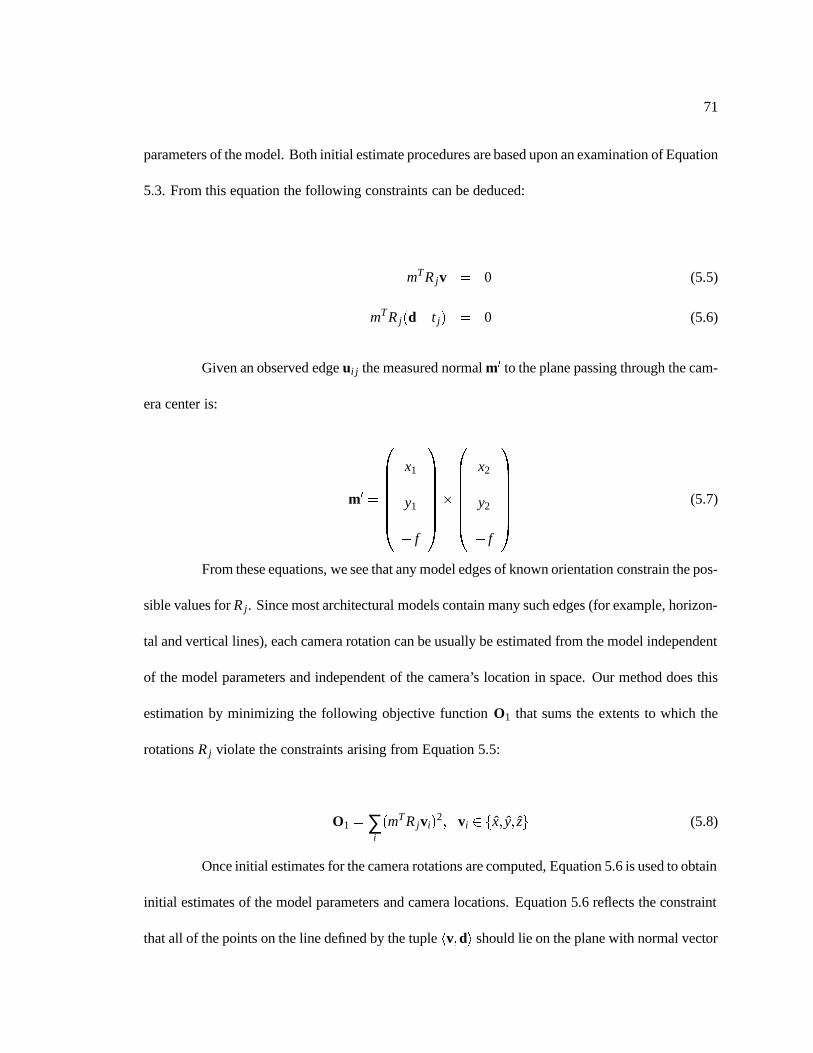
parameters of the model. Both initial estimate procedures are based upon an examination of Equation

5.3. From this equation the following constraints can be deduced:

mT R jv = 0 (5.5)

mT R j(d� t j) = 0 (5.6)

Given an observed edge ui j the measured normal m0 to the plane passing through the cam-

era center is:

m0 =

0BBBBBB@

x1

y1

� f

1CCCCCCA�

0BBBBBB@

x2

y2

� f

1CCCCCCA

(5.7)

From these equations, we see that any model edges of known orientation constrain the pos-

sible values for R j. Since most architectural models contain many such edges (for example, horizon-

tal and vertical lines), each camera rotation can be usually be estimated from the model independent

of the model parameters and independent of the camera’s location in space. Our method does this

estimation by minimizing the following objective function O1 that sums the extents to which the

rotations R j violate the constraints arising from Equation 5.5:

O1 = ∑i

(mT R jvi)2; vi 2 fx; y; zg (5.8)

Once initial estimates for the camera rotations are computed, Equation 5.6 is used to obtain

initial estimates of the model parameters and camera locations. Equation 5.6 reflects the constraint

that all of the points on the line defined by the tuple hv;di should lie on the plane with normal vector

72

m passing through the camera center. This constraint is expressed in the following objective function

O2 where Pi(X) and Qi(X) are expressions for the vertices of an edge of the model.

O2 = ∑i

(mT R j(Pi(X)� t j))2 +(mT R j(Qi(X)� t j))

2 (5.9)

In the special case where all of the block relations in the model have a known rotation, this

objective function becomes a simple quadratic form which is easily minimized by solving a set of

linear equations. This special case is actually quite often the case for any one particular building,

since very often all of the architectural elements are aligned on the same coordinate axis.

Once the initial estimate is obtained, the non-linear optimization over the entire parameter

space is applied to produce the best possible reconstruction. Typically, the optimization requires

fewer than ten iterations and adjusts the parameters of the model by at most a few percent from the

initial estimates. The edges of the recovered models typically conform to the original photographs

to within a pixel.

5.5 Results

5.5.1 The Campanile

Figs. 5.1 5.2 showed the results of using Facade to reconstruct a clock tower from a sin-

gle image. The model consists of twenty-three blocks recovered from seventy marked edges in one

image. The total modeling time was approximately two hours.

73

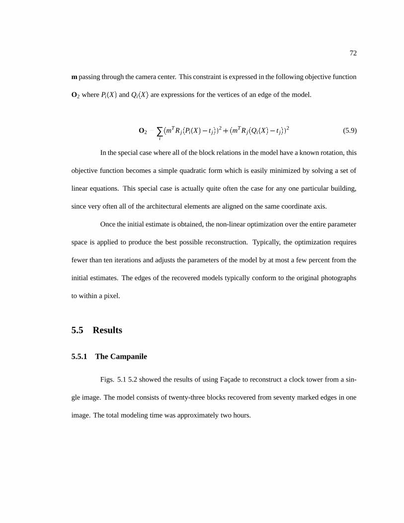
Figure 5.11: Three of twelve photographs used to reconstruct the entire exterior of University HighSchool in Urbana, Illinois. The superimposed lines indicate the edges the user has marked.

74

(a) (b)

(c)

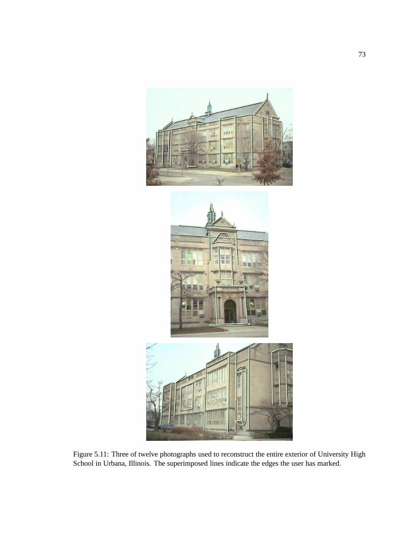
Figure 5.12: The high school model, reconstructed from twelve photographs. (a) Overhead view. (b)Rear view. (c) Aerial view showing the recovered camera positions. Two nearly coincident camerascan be observed in front of the building; their photographs were taken from the second story of abuilding across the street.

75

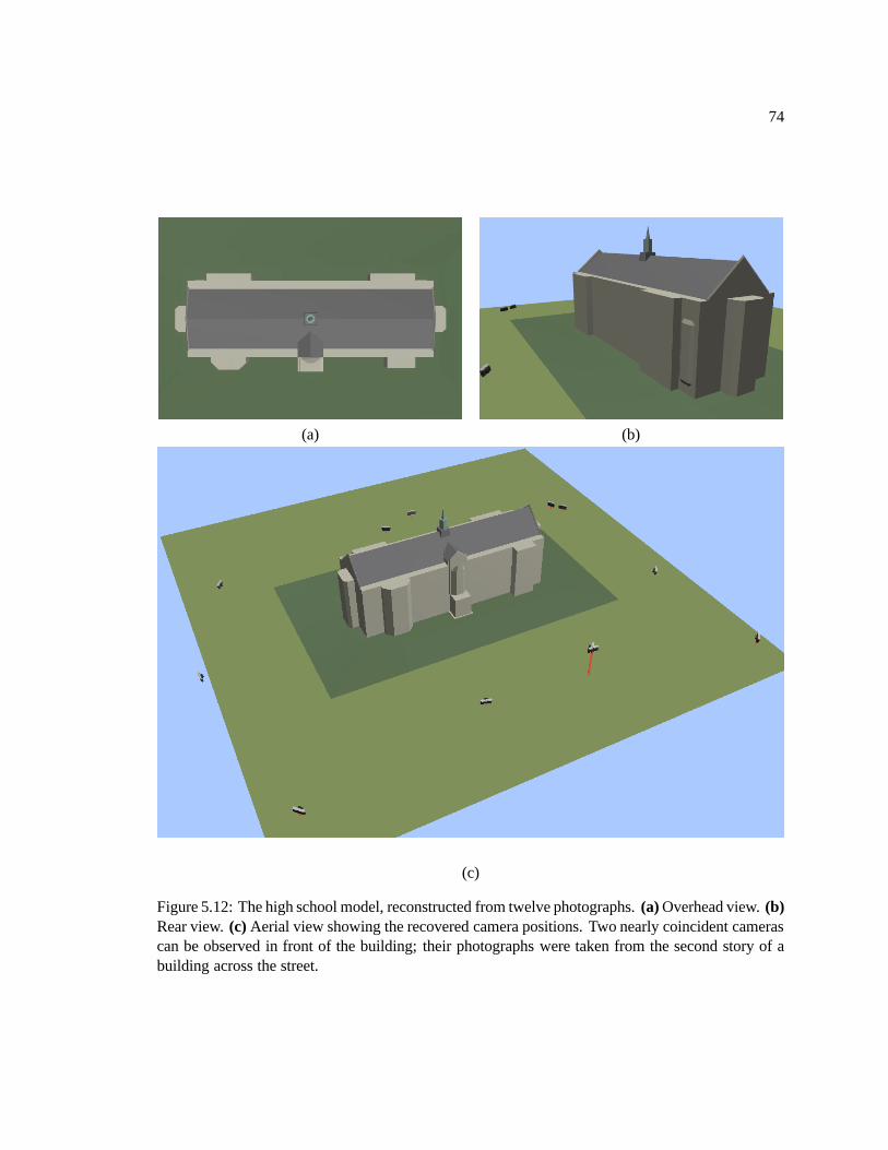
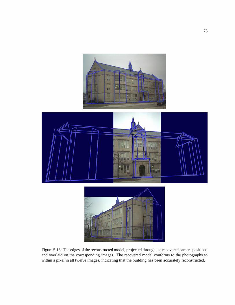
Figure 5.13: The edges of the reconstructed model, projected through the recovered camera positionsand overlaid on the corresponding images. The recovered model conforms to the photographs towithin a pixel in all twelve images, indicating that the building has been accurately reconstructed.

76

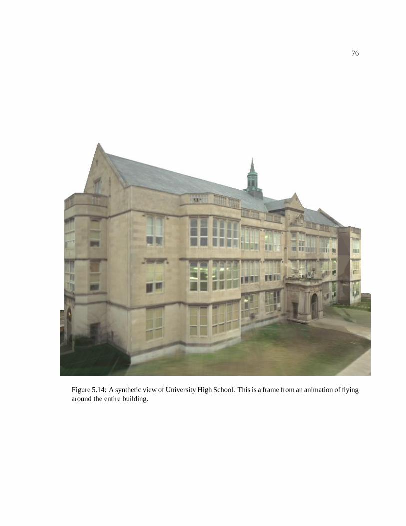
Figure 5.14: A synthetic view of University High School. This is a frame from an animation of flyingaround the entire building.

77

5.5.2 University High School

Figs. 5.11 and 5.12 show the results of using Facade to reconstruct a high school building

from twelve photographs. The model was originally constructed from just five images; the remain-

ing images were added to the project for purposes of generating renderings using the techniques of

Chapter 6. The photographs were taken with a calibrated 35mm still camera with a standard 50mm

lens and digitized with the PhotoCD process. Images at the 1536�1024 pixel resolution were pro-

cessed to correct for lens distortion, then filtered down to 768� 512 pixels for use in the modeling

system. Fig. 5.13 shows that the recovered model conforms to the photographs to within a pixel, in-

dicating an accurate reconstruction. Fig. 5.12 shows some views of the recovered model and camera

positions, and Fig. 5.14 shows a synthetic view of the building generated by the technique in Chapter

6. The total modeling time for all twelve images was approximately four hours.

The model was originally constructed using only approximate camera calibration data. By

using the building itself as a calibration object the focal length we originally used was later found to

be in error by 7%.

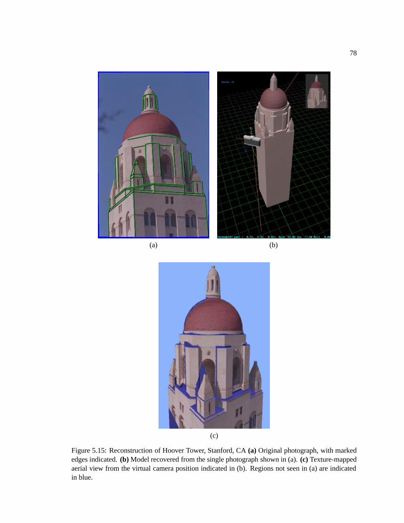
5.5.3 Hoover Tower

Fig. 5.15 shows the reconstruction of another tower from a single photograph. The dome

was modeled specially since at the time the reconstruction algorithm did not recover curved surfaces.

The user constrained a two-parameter hemisphere block to sit centered on top of the tower, and man-

ually adjusted its height and width to align with the photograph. This model took approximately four

hours to create.

78

(a) (b)

(c)

Figure 5.15: Reconstruction of Hoover Tower, Stanford, CA (a) Original photograph, with markededges indicated. (b) Model recovered from the single photograph shown in (a). (c) Texture-mappedaerial view from the virtual camera position indicated in (b). Regions not seen in (a) are indicatedin blue.

79

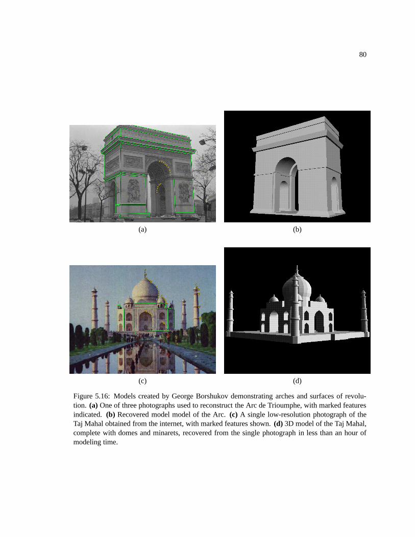
5.5.4 The Taj Mahal and the Arc de Trioumphe

As part of his Master’s degree research (in progress), George Borshukov showed that the

photogrammetric modeling methods presented here could be extended very naturally to arches and

surfaces of revolution. Two impressive examples from his work are shown in Fig. 5.16.

80

(a) (b)

(c) (d)

Figure 5.16: Models created by George Borshukov demonstrating arches and surfaces of revolu-tion. (a) One of three photographs used to reconstruct the Arc de Trioumphe, with marked featuresindicated. (b) Recovered model model of the Arc. (c) A single low-resolution photograph of theTaj Mahal obtained from the internet, with marked features shown. (d) 3D model of the Taj Mahal,complete with domes and minarets, recovered from the single photograph in less than an hour ofmodeling time.